modeling in the frequency domain - testbanktop.com · 2-2 chapter 2: modeling in the frequency...
TRANSCRIPT
T W O
Modeling in the Frequency Domain
SOLUTIONS TO CASE STUDIES CHALLENGES Antenna Control: Transfer Functions
Finding each transfer function:
Pot: Vi(s)θi(s) =
10π
;
Pre-Amp: Vp(s)Vi(s) = K;
Power Amp: Ea(s)Vp(s) =
150s+150
Motor: Jm = 0.05 + 5( 50250 )
2 = 0.25
Dm =0.01 + 3( 50250 )
2 = 0.13
KtRa
= 15
KtKb
Ra =
15
Therefore: θm(s)Ea(s) =
KtRaJm
s(s+1
Jm(Dm+
KtKbRa
)) =
0.8s(s+1.32)
And: θo(s)Ea(s) =
15
θm(s)Ea(s) =
0.16s(s+1.32)
Transfer Function of a Nonlinear Electrical Network
Writing the differential equation, d(i0 + δi)
dt+ 2(i0 +δi)2 − 5 = v(t) . Linearizing i2 about i0,
(i0
+δi)2
- i02
= 2i ⎮i=i
0
δi = 2i0δi.. Thus, (i
0+δi)
2= i
02
+ 2i0δi.

2-2 Chapter 2: Modeling in the Frequency Domain
Substituting into the differential equation yields, dδidt + 2i02 + 4i0δi - 5 = v(t). But, the
resistor voltage equals the battery voltage at equilibrium when the supply voltage is zero since
the voltage across the inductor is zero at dc. Hence, 2i02 = 5, or i0 = 1.58. Substituting into the linearized
differential equation, dδidt + 6.32δi = v(t). Converting to a transfer function,
δi(s)V(s) =
1s+6.32 . Using the
linearized i about i0, and the fact that vr(t) is 5 volts at equilibrium, the linearized vr(t) is vr(t) = 2i2 =
2(i0+δi)2 = 2(i02+2i0δi) = 5+6.32δi. For excursions away from equilibrium, vr(t) - 5 = 6.32δi = δvr(t).
Therefore, multiplying the transfer function by 6.32, yields, δVr(s)V(s) =
6.32s+6.32 as the transfer function
about v(t) = 0.
ANSWERS TO REVIEW QUESTIONS
1. Transfer function
2. Linear time-invariant
3. Laplace
4. G(s) = C(s)/R(s), where c(t) is the output and r(t) is the input.
5. Initial conditions are zero
6. Equations of motion
7. Free body diagram
8. There are direct analogies between the electrical variables and components and the mechanical variables
and components.
9. Mechanical advantage for rotating systems
10. Armature inertia, armature damping, load inertia, load damping
11. Multiply the transfer function by the gear ratio relating armature position to load position.
12. (1) Recognize the nonlinear component, (2) Write the nonlinear differential equation, (3) Select the
equilibrium solution, (4) Linearize the nonlinear differential equation, (5) Take the Laplace transform of
the linearized differential equation, (6) Find the transfer function.
SOLUTIONS TO PROBLEMS
1.
a. F(s) = e− stdt0
∞
∫ = −1s
e−st
0
∞
=1s
b. F(s) = te− stdt0
∞
∫ =e−st
s2 (−st −1) 0∞ =
−(st +1)s2est
0
∞

Solutions to Problems 2-3
Using L'Hopital's Rule
F(s) t → ∞ =−s
s 3estt →∞
= 0. Therefore, F(s) =1s2 .
c. F(s) = sinωt e− stdt0
∞
∫ =e− st
s2 + ω 2 (−ssinωt − ω cosωt)0
∞
=ω
s2 +ω 2
d. F(s) = cosωt e− stdt0
∞
∫ =e− st
s2 + ω 2 (−scosωt + ω sinωt)0
∞
=s
s2 +ω 2
2.
a. Using the frequency shift theorem and the Laplace transform of sin ωt, F(s) = ω
(s+a)2+ω2 .
b. Using the frequency shift theorem and the Laplace transform of cos ωt, F(s) = (s+a)
(s+a)2+ω2 .
c. Using the integration theorem, and successively integrating u(t) three times, ⌡⌠dt = t; ⌡⌠tdt = t22 ;
⌡⌠t2
2dt = t36 , the Laplace transform of t3u(t), F(s) =
6s4 .
3. a. The Laplace transform of the differential equation, assuming zero initial conditions,
is, (s+7)X(s) = 5s
s2+22 . Solving for X(s) and expanding by partial fractions,
Or,
Taking the inverse Laplace transform, x(t) = - 3553 e-7t + (
3553 cos 2t +
1053 sin 2t).
b. The Laplace transform of the differential equation, assuming zero initial conditions, is,
(s2+6s+8)X(s) = 15
s2 + 9.
Solving for X(s)
X(s) =15
(s2 + 9)(s2 + 6s + 8)
and expanding by partial fractions,
X(s) = −365
6s +19
9
s2 + 9−
310
1s + 4
+1526
1s + 2
2-4 Chapter 2: Modeling in the Frequency Domain
Taking the inverse Laplace transform,
x(t) = −1865
cos(3t) −165
sin(3t) −3
10e−4t +
1526
e−2t
c. The Laplace transform of the differential equation is, assuming zero initial conditions,
(s2+8s+25)x(s) = 10s
. Solving for X(s)
X s = 10s s 2 + 8 s + 25
and expanding by partial fractions,
X s = 25
1s - 2
5
1 s + 4 + 49
9
s + 42 + 9 Taking the inverse Laplace transform,
x(t) =25
− e−4t 815
sin(3t) +25
cos(3t )⎛ ⎝
⎞ ⎠
4.
a. Taking the Laplace transform with initial conditions, s2X(s)-4s+4+2sX(s)-8+2X(s) = 2
s2+22 .
Solving for X(s),
X(s) = 3 2
2 2
4 4 16 18( 4)( 2 2)
s s ss s s
+ + ++ + +
.
Expanding by partial fractions
2 2 2
1s 21 1 21(s 1) 22X(s)5 s 2 5 (s 1) 1
+ + +⎛ ⎞ ⎛ ⎞= − +⎜ ⎟ ⎜ ⎟+ + +⎝ ⎠ ⎝ ⎠
Therefore, 1 2 1( ) 21 cos sin sin 2 cos 25 21 2
t tx t e t e t t t− −⎡ ⎤= + − −⎢ ⎥⎣ ⎦
b. Taking the Laplace transform with initial conditions, s2X(s)-4s-1+2sX(s)-8+X(s) = 5
s+2 + 1s2 .
Solving for X(s), 4 3 2
2 2
4 17 23 2( )( 1) ( 2)
s s s sX ss s s+ + + +
=+ +
2 2
1 2 11 1 5( )( 1) ( 1) ( 2)
X ss s s s s
= − + + ++ + +
Therefore 2( ) 2 11 5t t tx t t te e e− − −= − + + + .
c. Taking the Laplace transform with initial conditions, s2X(s)-s-2+4X(s) = 2s3 . Solving for X(s),

Solutions to Problems 2-5
4 3
3 2
2 3 2( )( 4)
s sX ss s
+ +=
+
2 3
17 3 *2 1/ 2 1/ 88 2( )4
sX s
s s s
+= + −
+
Therefore 217 3 1 1( ) cos 2 sin 28 2 4 8
x t t t t= + + − .
5. Program: syms t 'a' theta=45*pi/180 f=8*t^2*cos(3*t+theta); pretty(f) F=laplace(f); F=simple(F); pretty(F) 'b' theta=60*pi/180 f=3*t*exp(-2*t)*sin(4*t+theta); pretty(f) F=laplace(f); F=simple(F); pretty(F) Computer response:
ans = a theta = 0.7854 2 / PI \ 8 t cos| -- + 3 t | \ 4 / 1/2 2 8 2 (s + 3) (s - 12 s + 9) ------------------------------ 2 3 (s + 9) ans = b theta = 1.0472

2-6 Chapter 2: Modeling in the Frequency Domain
/ PI \ 3 t sin| -- + 4 t | exp(-2 t) \ 3 / 1/2 2 1/2 1/2 3 3 s 12 s + 6 3 s - 18 3 + --------- + 24 2 ------------------------------------------ 2 2 (s + 4 s + 20) 6.
Program: syms s 'a' G=(s^2+3*s+10)*(s+5)/[(s+3)*(s+4)*(s^2+2*s+100)]; pretty(G) g=ilaplace(G); pretty(g) 'b' G=(s^3+4*s^2+2*s+6)/[(s+8)*(s^2+8*s+3)*(s^2+5*s+7)]; pretty(G) g=ilaplace(G); pretty(g) Computer response:
ans = a 2 (s + 5) (s + 3 s + 10) -------------------------------- 2 (s + 3) (s + 4) (s + 2 s + 100) / 1/2 1/2 \ | 1/2 11 sin(3 11 t) | 5203 exp(-t) | cos(3 11 t) - ------------------| 20 exp(-3 t) 7 exp(-4 t) \ 57233 / ------------ - ----------- + --------------------------------------------------- 103 54 5562
Solutions to Problems 2-7
ans = b 3 2 s + 4 s + 2 s + 6 ------------------------------------- 2 2 (s + 8) (s + 8 s + 3) (s + 5 s + 7) / 1/2 1/2 \ | 1/2 4262 13 sinh(13 t) | 1199 exp(-4 t) | cosh(13 t) - ------------------------ | \ 15587 / ----------------------------------------------------------- - 417 / / 1/2 \ \ | 1/2 | 3 t | | | / 1/2 \ 131 3 sin| ------ | | / 5 t \ | | 3 t | \ 2 / | 65 exp| - --- | | cos| ------ | + ---------------------- | \ 2 / \ \ 2 / 15 / 266 exp(-8 t) ---------------------------------------------------------- - ------------- 4309 93 7.
The Laplace transform of the differential equation, assuming zero initial conditions, is, (s3+5s2+7s+1)Y(s) = (s3+6s2+2s+8)X(s).
Solving for the transfer function, Y(s)X(s)
= 3 2
3 2
6 2 85 7 1
s s ss s s
+ + ++ + +
.
8. a. Cross multiplying, (s2+7s+11)X(s) = 9F(s).
Taking the inverse Laplace transform, d2 xdt2 + 7
dxdt
+ 11x = 9f(t).
b. Cross multiplying after expanding the denominator, (s2+23s+132)X(s) = 7F(s).
Taking the inverse Laplace transform, d2 xdt2 + 23
dxdt
+ 132x =7f(t).
c. Cross multiplying, (s3+10s2+11s+18)X(s) = (s+2)F(s).
Taking the inverse Laplace transform, d3 xdt3 + 10
d2 xdt2 + 11
dxdt
+ 18x = df (t)
dt+2f(t).
9.
The transfer function is C(s)R(s)
= 5 4 3 2
6 5 4 3 2
3 4 5 38 3 2 3 3
s s s ss s s s s
+ + + ++ + + + +
.
Cross multiplying, (s6+8s5+3s4+2s3+3s2+3)C(s) = (s5+3s4+4s3+5s2+3)R(s).
Taking the inverse Laplace transform assuming zero initial conditions, d6cdt6 + 8
d5cdt5 + 3
d 4cdt4 + 2
d3cdt3 + 3
d2cdt2 + 5c =
d5rdt5 + 3
d 4rdt4 + 4
d3rdt3 + 5
d2rdt2 + 4r.
10.
The transfer function is C(s)R(s)
= s4 + 2s3 + 5s2 + s +1
s5 + 3s 4 + 2s3 + 4s2 + 5s + 2.
2-8 Chapter 2: Modeling in the Frequency Domain
Cross multiplying, (s5+3s4+2s3+4s2+5s+2)C(s) = (s4+2s3+5s2+s+1)R(s).
Taking the inverse Laplace transform assuming zero initial conditions, d5cdc5 + 3
d 4cdt4 + 2
d3cdt3 + 4
d2cdt2 + 5
dcdt
+ 2c = d 4rdt4 + 2
d3rdt3 + 5
d2rdt2 +
drdt
+ r.
Substituting r(t) = t3, d5cdc5 + 3
d 4cdt4 + 2
d3cdt3 + 4
d2cdt2 + 5
dcdt
+ 2c
= 18δ(t) + (36 + 90t + 9t2 + 3t3) u(t).
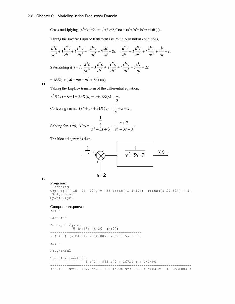
11. Taking the Laplace transform of the differential equation,
2 1s X( ) s 1 3sX(s) 3 3X(s)s
s − + + − + = .
Collecting terms, 2 1(s 3s 3)X(s) 2s
s+ + = + + .
Solving for X(s), X(s) = 2
1
3 3s
s s+ ++ 2
23 3
ss s
++ +
.
The block diagram is then,
12.
Program: 'Factored' Gzpk=zpk([-15 -26 -72],[0 -55 roots([1 5 30])' roots([1 27 52])'],5) 'Polynomial' Gp=tf(Gzpk) Computer response: ans = Factored Zero/pole/gain: 5 (s+15) (s+26) (s+72) -------------------------------------------- s (s+55) (s+24.91) (s+2.087) (s^2 + 5s + 30) ans = Polynomial Transfer function: 5 s^3 + 565 s^2 + 16710 s + 140400 -------------------------------------------------------------------- s^6 + 87 s^5 + 1977 s^4 + 1.301e004 s^3 + 6.041e004 s^2 + 8.58e004 s
Solutions to Problems 2-9
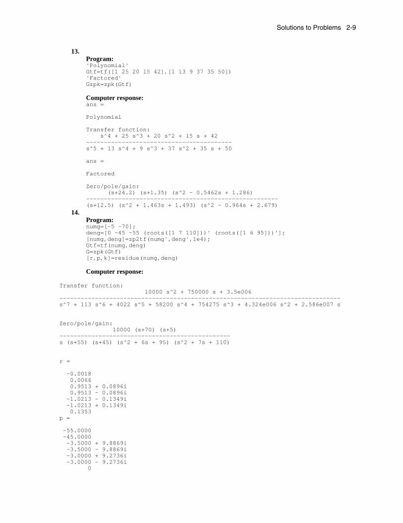
13. Program: 'Polynomial' Gtf=tf([1 25 20 15 42],[1 13 9 37 35 50]) 'Factored' Gzpk=zpk(Gtf) Computer response: ans = Polynomial Transfer function: s^4 + 25 s^3 + 20 s^2 + 15 s + 42 ----------------------------------------- s^5 + 13 s^4 + 9 s^3 + 37 s^2 + 35 s + 50 ans = Factored Zero/pole/gain: (s+24.2) (s+1.35) (s^2 - 0.5462s + 1.286) ------------------------------------------------------ (s+12.5) (s^2 + 1.463s + 1.493) (s^2 - 0.964s + 2.679)
14. Program: numg=[-5 -70]; deng=[0 -45 -55 (roots([1 7 110]))' (roots([1 6 95]))']; [numg,deng]=zp2tf(numg',deng',1e4); Gtf=tf(numg,deng) G=zpk(Gtf) [r,p,k]=residue(numg,deng) Computer response:
Transfer function: 10000 s^2 + 750000 s + 3.5e006 ------------------------------------------------------------------------------- s^7 + 113 s^6 + 4022 s^5 + 58200 s^4 + 754275 s^3 + 4.324e006 s^2 + 2.586e007 s Zero/pole/gain: 10000 (s+70) (s+5) ------------------------------------------------ s (s+55) (s+45) (s^2 + 6s + 95) (s^2 + 7s + 110) r = -0.0018 0.0066 0.9513 + 0.0896i 0.9513 - 0.0896i -1.0213 - 0.1349i -1.0213 + 0.1349i 0.1353 p = -55.0000 -45.0000 -3.5000 + 9.8869i -3.5000 - 9.8869i -3.0000 + 9.2736i -3.0000 - 9.2736i 0
2-10 Chapter 2: Modeling in the Frequency Domain
k = []
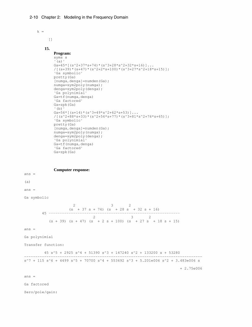
15.
Program: syms s '(a)' Ga=45*[(s^2+37*s+74)*(s^3+28*s^2+32*s+16)]... /[(s+39)*(s+47)*(s^2+2*s+100)*(s^3+27*s^2+18*s+15)]; 'Ga symbolic' pretty(Ga) [numga,denga]=numden(Ga); numga=sym2poly(numga); denga=sym2poly(denga); 'Ga polynimial' Ga=tf(numga,denga) 'Ga factored' Ga=zpk(Ga) '(b)' Ga=56*[(s+14)*(s^3+49*s^2+62*s+53)]... /[(s^2+88*s+33)*(s^2+56*s+77)*(s^3+81*s^2+76*s+65)]; 'Ga symbolic' pretty(Ga) [numga,denga]=numden(Ga); numga=sym2poly(numga); denga=sym2poly(denga); 'Ga polynimial' Ga=tf(numga,denga) 'Ga factored' Ga=zpk(Ga) Computer response:
ans = (a) ans = Ga symbolic 2 3 2 (s + 37 s + 74) (s + 28 s + 32 s + 16) 45 ----------------------------------------------------------- 2 3 2 (s + 39) (s + 47) (s + 2 s + 100) (s + 27 s + 18 s + 15) ans = Ga polynimial Transfer function: 45 s^5 + 2925 s^4 + 51390 s^3 + 147240 s^2 + 133200 s + 53280 -------------------------------------------------------------------------------- s^7 + 115 s^6 + 4499 s^5 + 70700 s^4 + 553692 s^3 + 5.201e006 s^2 + 3.483e006 s + 2.75e006 ans = Ga factored Zero/pole/gain:

Solutions to Problems 2-11
45 (s+34.88) (s+26.83) (s+2.122) (s^2 + 1.17s + 0.5964) ----------------------------------------------------------------- (s+47) (s+39) (s+26.34) (s^2 + 0.6618s + 0.5695) (s^2 + 2s + 100) ans = (b) ans = Ga symbolic 3 2 (s + 14) (s + 49 s + 62 s + 53) 56 ---------------------------------------------------------- 2 2 3 2 (s + 88 s + 33) (s + 56 s + 77) (s + 81 s + 76 s + 65) ans = Ga polynimial Transfer function: 56 s^4 + 3528 s^3 + 41888 s^2 + 51576 s + 41552 -------------------------------------------------------------------------------- s^7 + 225 s^6 + 16778 s^5 + 427711 s^4 + 1.093e006 s^3 + 1.189e006 s^2 + 753676 s + 165165 ans = Ga factored Zero/pole/gain: 56 (s+47.72) (s+14) (s^2 + 1.276s + 1.111) --------------------------------------------------------------------------- (s+87.62) (s+80.06) (s+54.59) (s+1.411) (s+0.3766) (s^2 + 0.9391s + 0.8119)
16.
a. Writing the node equations, 2 0o i oo
V V V Vs s−
+ + = . Solve for
12
1o
i
VV s
=+
.
b. Thevenizing,

2-12 Chapter 2: Modeling in the Frequency Domain
Using voltage division,
2( )( ) 1 12
2
io
V s sV ss
s
=+ +
. Thus, 2
( ) 2( ) 2 2
o
i
V sV s s s
=+ +
17. a.
Writing mesh equations
(2s+2)I1(s) –2 I2(s) = Vi(s)
-2I1(s) + (2s+4)I2(s) = 0
But from the second equation, I1(s) = (s+2)I2(s). Substituting this in the first equation yields,
(2s+2)(s+2)I2(s) –2 I2(s) = Vi(s) or
I2(s)/Vi(s) = 1/(2s2 + 4s + 2)
But, VL(s) = sI2(s). Therefore, VL(s)/Vi(s) = s/(2s2 + 4s + 2).
b.
i1(t) i2(t)
1 2
1
2 1(4 ) ( ) (2 ) ( ) ( )
1 1(2 ) ( ) (4 2 ) 0
I s I s V ss s
I s ss s
+ − + =
− + + + + =
2
2
2
2
2
2
Solutions to Problems 2-13
Solving for I2(s):
2 2
2
4 2 ( )
(2 1) 0 ( )( )4 2 (2 1) 4 6 1
(2 1) (2 4 1)
s V sss
sV ssI ss s s ss ss s ss s
+
− +
= =+ − + + +
− + + +
Therefore, 2
22
( ) 2 ( ) 2( ) ( ) 4 6 1
LV s sI s sV s V s s s
= =+ +
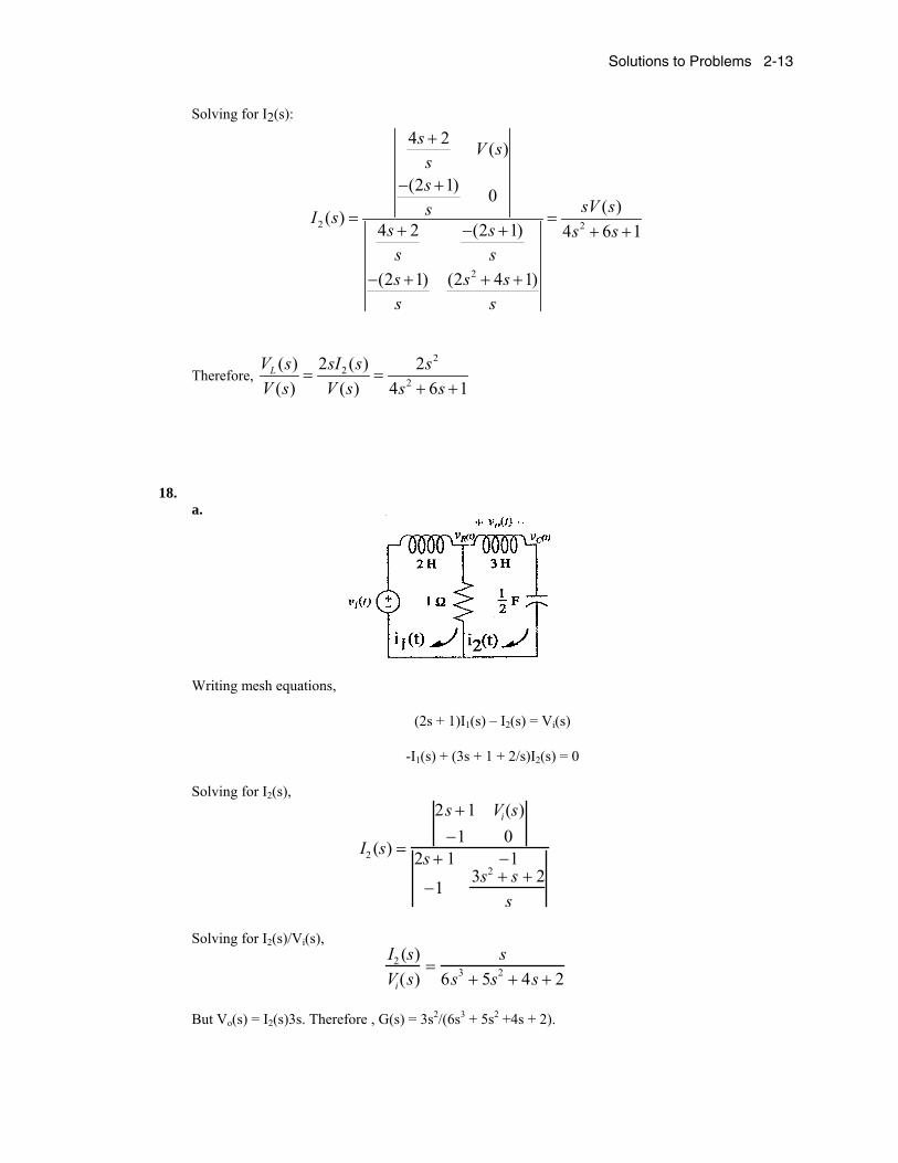
18.
a.
Writing mesh equations,
(2s + 1)I1(s) – I2(s) = Vi(s)
-I1(s) + (3s + 1 + 2/s)I2(s) = 0
Solving for I2(s),
I2 (s) =
2s +1 Vi(s)−1 0
2s + 1 −1
−13s2 + s + 2
s
Solving for I2(s)/Vi(s), I2 (s)Vi(s)
=s
6s3 + 5s2 + 4s + 2
But Vo(s) = I2(s)3s. Therefore , G(s) = 3s2/(6s3 + 5s2 +4s + 2).

2-14 Chapter 2: Modeling in the Frequency Domain
b. Transforming the network yields,
Writing the loop equations,
(s +s
s2 +1)I1(s) −
ss2 +1
I2 (s) − sI3(s) = Vi(s)
−s
s2 +1I1(s) + (
ss2 +1
+1 +1s)I2 (s) − I3 (s) = 0
− sI1(s) − I2 (s) + (2s +1)I3 (s) = 0 Solving for I2(s),
I2 (s) =s(s2 + 2s + 2)
s 4 + 2s 3 + 3s2 + 3s + 2Vi(s)
But, Vo(s) = I2(s)
s = (s 2 + 2s + 2)
s 4 + 2s3 + 3s2 + 3s + 2Vi(s) . Therefore,
Vo (s)Vi(s)
=s2 + 2s + 2
s4 + 2s3 + 3s2 + 3s + 2
19.
a. Writing the nodal equations yields,
VR(s) −Vi(s)
2s+ VR(s)
1+ VR (s) − VC (s)
3s= 0
−1
3sVR(s) +
12
s +1
3s⎛ ⎝
⎞ ⎠ VC (s) = 0
Rewriting and simplifying,

Solutions to Problems 2-15
6s + 56s
VR(s) − 13s
VC (s) = 12s
Vi(s)
−13s
VR(s) +3s2 + 2
6s⎛ ⎝ ⎜ ⎞
⎠ VC (s) = 0
Solving for VR(s) and VC(s),
VR(s) =
12s
Vi (s) −13s
03s2 + 2
6s6s + 5
6s− 1
3s− 1
3s3s2 + 2
6s
; VC (s) =
6s + 56s
12s
Vi(s)
−13s
0
6s + 56s
− 13s
− 13s
3s 2 + 26s
Solving for Vo(s)/Vi(s) Vo (s)Vi(s)
=VR(s) − VC (s)
Vi(s)=
3s2
6s3 + 5s2 + 4s + 2
b. Writing the nodal equations yields,
(V1(s) − Vi (s))
s+ (s 2 +1)
sV1(s) + (V1(s) − Vo (s)) = 0
(Vo (s) − V1(s)) + sVo(s) +(Vo (s) − Vi (s))
s= 0
Rewriting and simplifying,
(s + 2s
+1)V1(s) − Vo (s) = 1sVi(s)
V1(s) + (s +1s
+ 1)Vo (s) =1s
Vi (s)
Solving for Vo(s)
Vo(s) = (s 2 + 2s + 2)
s 4 + 2s3 + 3s2 + 3s + 2Vi(s) .
Hence,
2-16 Chapter 2: Modeling in the Frequency Domain
Vo (s)Vi(s)
=(s2 + 2s + 2)
s4 + 2s3 + 3s2 + 3s + 2
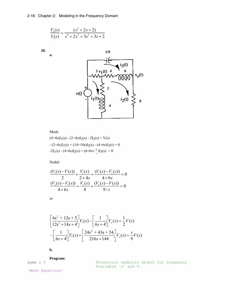
20.
a.
Mesh: (4+4s)I1(s) - (2+4s)I2(s) - 2I3(s) = V(s)
- (2+4s)I1(s) + (14+10s)I2(s) - (4+6s)I3(s) = 0 -2I1(s) - (4+6s)I2(s) + (6+6s+ 9
s)I3(s) = 0
Nodal:
11 1 ( ( ) ( ))( ( ) ( )) ( ) 02 2 4 4 6
oV s V sV s V s V ss s
−−+ + =
+ +
1( ( ) ( )) ( ) ( ( ) ( )) 04 6 8 9 /
o o oV s V s V s V s V ss s
− −+ + =
+
or
2
12
6s + 12s + 5 1 1( ) ( ) ( )12s 14 4 6 4 2oV s V s V s
s s⎡ ⎤ ⎡ ⎤− =⎢ ⎥ ⎢ ⎥+ + +⎣ ⎦⎣ ⎦
2
11 24s + 43s + 54( ) ( ) ( )
6 4 216 144 9osV s V s V s
s s⎡ ⎤⎡ ⎤− + =⎢ ⎥⎢ ⎥+ +⎣ ⎦ ⎣ ⎦
b. Program:
syms s V %Construct symbolic object for frequency %variable 's' and V. 'Mesh Equations'
1/9
2 4 6
2
48
Solutions to Problems 2-17
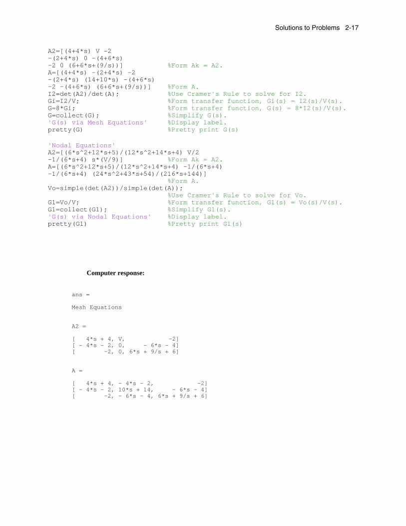
A2=[(4+4*s) V -2 -(2+4*s) 0 -(4+6*s) -2 0 (6+6*s+(9/s))] %Form Ak = A2. A=[(4+4*s) -(2+4*s) -2 -(2+4*s) (14+10*s) -(4+6*s) -2 -(4+6*s) (6+6*s+(9/s))] %Form A. I2=det(A2)/det(A); %Use Cramer's Rule to solve for I2. Gi=I2/V; %Form transfer function, Gi(s) = I2(s)/V(s). G=8*Gi; %Form transfer function, G(s) = 8*I2(s)/V(s). G=collect(G); %Simplify G(s). 'G(s) via Mesh Equations' %Display label. pretty(G) %Pretty print G(s) 'Nodal Equations' A2=[(6*s^2+12*s+5)/(12*s^2+14*s+4) V/2 -1/(6*s+4) s*(V/9)] %Form Ak = A2. A=[(6*s^2+12*s+5)/(12*s^2+14*s+4) -1/(6*s+4) -1/(6*s+4) (24*s^2+43*s+54)/(216*s+144)] %Form A. Vo=simple(det(A2))/simple(det(A)); %Use Cramer's Rule to solve for Vo. G1=Vo/V; %Form transfer function, G1(s) = Vo(s)/V(s). G1=collect(G1); %Simplify G1(s). 'G(s) via Nodal Equations' %Display label. pretty(G1) %Pretty print G1(s)
Computer response:
ans = Mesh Equations A2 = [ 4*s + 4, V, -2] [ - 4*s - 2, 0, - 6*s - 4] [ -2, 0, 6*s + 9/s + 6] A = [ 4*s + 4, - 4*s - 2, -2] [ - 4*s - 2, 10*s + 14, - 6*s - 4] [ -2, - 6*s - 4, 6*s + 9/s + 6]

2-18 Chapter 2: Modeling in the Frequency Domain
ans = G(s) via Mesh Equations 3 2 48 s + 96 s + 112 s + 36 ---------------------------- 3 2 48 s + 150 s + 220 s + 117 ans = Nodal Equations A2 = [ (6*s^2 + 12*s + 5)/(12*s^2 + 14*s + 4), V/2] [ -1/(6*s + 4), (V*s)/9] A = [ (6*s^2 + 12*s + 5)/(12*s^2 + 14*s + 4), -1/(6*s + 4)] [ -1/(6*s + 4), (24*s^2 + 43*s + 54)/(216*s + 144)] ans = G(s) via Nodal Equations 3 2 48 s + 96 s + 112 s + 36 ---------------------------- 3 2 48 s + 150 s + 220 s + 117 21.
a.
65
1
65
2
10( ) 4 10210( ) 2 102
Z ss
Z ss
= × +
= × +
Therefore,
2
1
( ) 2 5( ) 4 5
Z s sZ s s
+− = −
+

Solutions to Problems 2-19
b.
5 51
1 ( 1)( ) 10 1 10 sZ ss s
+⎛ ⎞= + =⎜ ⎟⎝ ⎠
( )5 5
25 ( 10)( ) 10 1 10
5 5sZ s
s s+⎛ ⎞= + =⎜ ⎟+ +⎝ ⎠
Therefore,
( )( )( )
2
1
10( )( ) 1 5
s sZ sZ s s s
+− = −
+ +
22. a.
1 6
2 6
1( ) 4000004*10
1( ) 1100004*10
Z ss
Z ss
−
−
= +
= +
Therefore,
1 2
1
( ) ( ) ( 0.98)( ) 1.275( ) ( 0.625)
Z s Z s sG sZ s s
+ += =
+
b. 11
51 6
5
9
52 6
3
10
( ) 4 100.25 104 10
1027.5( ) 6 10
0.25 10110 10
sZ s xxxs
sZ s xxxs
= ++
= ++
Therefore,
21 2
21
( ) ( ) 2640 8420 4275( ) 1056 3500 2500
Z s Z s s sZ s s s
+ + +=
+ +
23. Writing the equations of motion, where x2(t) is the displacement of the right member of springr,
(3s2+2s+5)X1(s) -5X2(s) = 0
-5X1(s) +5X2(s) = F(s)
Adding the equations,
(3s2+2s)X1(s) = F(s)
2-20 Chapter 2: Modeling in the Frequency Domain
From which, 1X (s) 1 1/ 3F(s) s(3s 2) s(s 2 / 3)
= =+ +
.
24. Writing the equations of motion,
21 2
21 2
(2 1) ( ) ( 1) ( ) ( )( 1) ( ) (2 1) ( ) 0s s X s s X s F ss X s s s X s
+ + − + =
− + + + + =
Solving for X2(s), 2
2 2 22
2
(2 1) ( )( 1) 0 ( 1) ( )( )
4 ( 1)(2 1) ( 1)( 1) (2 1)
s s F ss s F sX s
s s ss s ss s s
⎡ ⎤+ +⎢ ⎥− + +⎣ ⎦= =
+ +⎡ ⎤+ + − +⎢ ⎥− + + +⎣ ⎦
From which,
22 2
( ) ( 1)( ) 4 ( 1)
X s sF s s s s
+=
+ +.
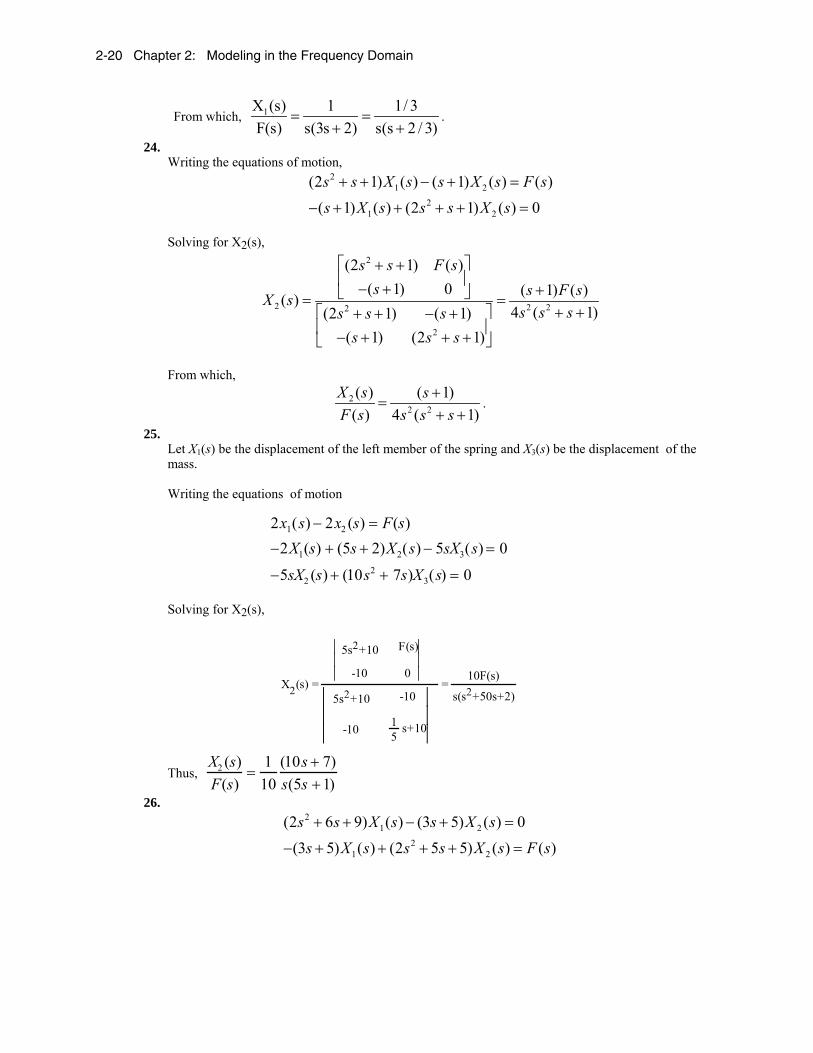
25. Let X1(s) be the displacement of the left member of the spring and X3(s) be the displacement of the mass. Writing the equations of motion
2x1(s) − 2x2 (s) = F(s)−2X1(s) + (5s + 2)X2(s) − 5sX3(s) = 0
−5sX2 (s) + (10s2 + 7s)X3(s) = 0
Solving for X2(s),
X2(s) = ⎪⎪⎪
5s2+10 -10
-10 51 s+10
⎪⎪⎪
⎪⎪⎪
5s2+10 F(s)
-10 0
⎪⎪⎪
= s(s2+50s+2)
10F(s)
Thus, X2 (s)F(s)
=110
(10s + 7)s(5s +1)
26. 2
1 22
1 2
(2 6 9) ( ) (3 5) ( ) 0(3 5) ( ) (2 5 5) ( ) ( )s s X s s X s
s X s s s X s F s+ + − + =
− + + + + =

Solutions to Problems 2-21
Solving for X1(s); 2
1 4 3 22
2
0 (3 5)( ) (2 5 5) (3 5) ( )( )
2 17 44 45 20(2 6 9) (3 5)(3 5) (2 5 5)
sF s s s s F sX s
s s s ss s ss s s
− +⎡ ⎤⎢ ⎥+ + +⎣ ⎦= =
+ + + +⎡ ⎤+ + − +⎢ ⎥− + + +⎣ ⎦
Thus G(s) = X1(s)/F(s) = 4 3 2
(3 5)4 22 49 45 20
ss s s s
++ + + +
27. Writing the equations of motion,
21 2
21 2 3
22 3
(2 2 6) ( ) 2 ( ) 02 ( ) (4 2 6) ( ) 6 ( ) ( )
6 ( ) (4 2 4) ( ) 0
s s X s sX ssX s s s X s X s F s
X s s s X s
+ + − =
− + + + − =
− + + + =
Solving for X3(s),
( )
2
2
2
3 6 5 4 3 22
2
2
(2 2 6) 2 02 (4 4 6) ( ) 3 3 ( )0 6 0 2( )
4 12 32 46 47 27 9(2 2 6) 2 02 (4 4 6) 60 6 (4 2 4)
s s ss s s F s
s s F sX s
s s s s s ss s ss s s
s s
+ + −− + +
+ +−= =
+ + + + + −+ + −− + + −
− + +
From which, ( )2
36 5 4 3
3 3( ) 2( ) 4 12 32 46 27 9
s sX sF s s s s s s
+ +=
+ + + + −.
28. a.
21 2 32
1 2 3
1 2 3
(4s 8s 5)X (s) 8sX (s) 5X (s) F(s)
8sX (s) (4s 16s)X (s) 4sX (s) 05X (s) 4sX (s) (4s 5)X (s) 0
+ + − − =
− + + − =− − + + =
Solving for X3(s),
2
2 2
3
(4s 8s 5) 8s F(s)8s (4s 16s) 0 8s (4s 16s)
F(s)5 4s 0 5 4
X (s)s
+ + −− + − +− − − −
= =∆ ∆
or,

2-22 Chapter 2: Modeling in the Frequency Domain
33 2
X (s) 13s 20F(s) 4s(4s 25s 43s 15)
+=
+ + + b.
21 2 3
21 2 3
1 2 3
(8s 4s 16) X (s) (4s 1) X (s) 15X (s) 0
(4s 1) X (s) (3s 20s 1) X (s) 16sX (s) F(s)15X (s) 16sX (s) (16s 15) X (s) 0
+ + − + − =
− + + + + − =− − + + =
Solving for X3(s),
2
2 2
3
(8s 4s 16) -(4s+1) 0(4s+1) (3s 20s+1) F(s) (8s 4s 16) -(4s+1)
-F(s)15 -16s 0 15 16
X (s)s
+ +− + + +
− − −= =
∆ ∆
or
X3(s)F(s) =
3 2
5 4 3 2
128 64 316 15384 1064 3476 165
s s ss s s s
+ + ++ + +
29. Writing the equations of motion,
21 2 3
21 2 3
21 2
(4 4 7) ( ) 3 ( ) 2 ( ) 0
3 ( ) (2 5 3) ( ) 5 ( ) ( )
2 ( ) 5 ( ) (3 7 2) 0
s s X s X s sX s
X s s s X s sX s F s
sX s sX s s s
+ + − − =
− + + + − =
− − + + + =
30.
a.
Writing the equations of motion,
Solutions to Problems 2-23
2
1 22
1 2
(5 10 9) ( ) (2 9) ( ) 0(2 9) ( ) (3 2 14) ( ) ( )s s s s s
s s s s s T sθ θ
θ θ
+ + − + =
− + + + + =
b. Defining
θ1(s) = rotation of J1
θ2 (s) = rotation between K1 and D1
θ3(s) = rotation of J3
θ4 (s) = rotation of right - hand side of K2
the equations of motion are
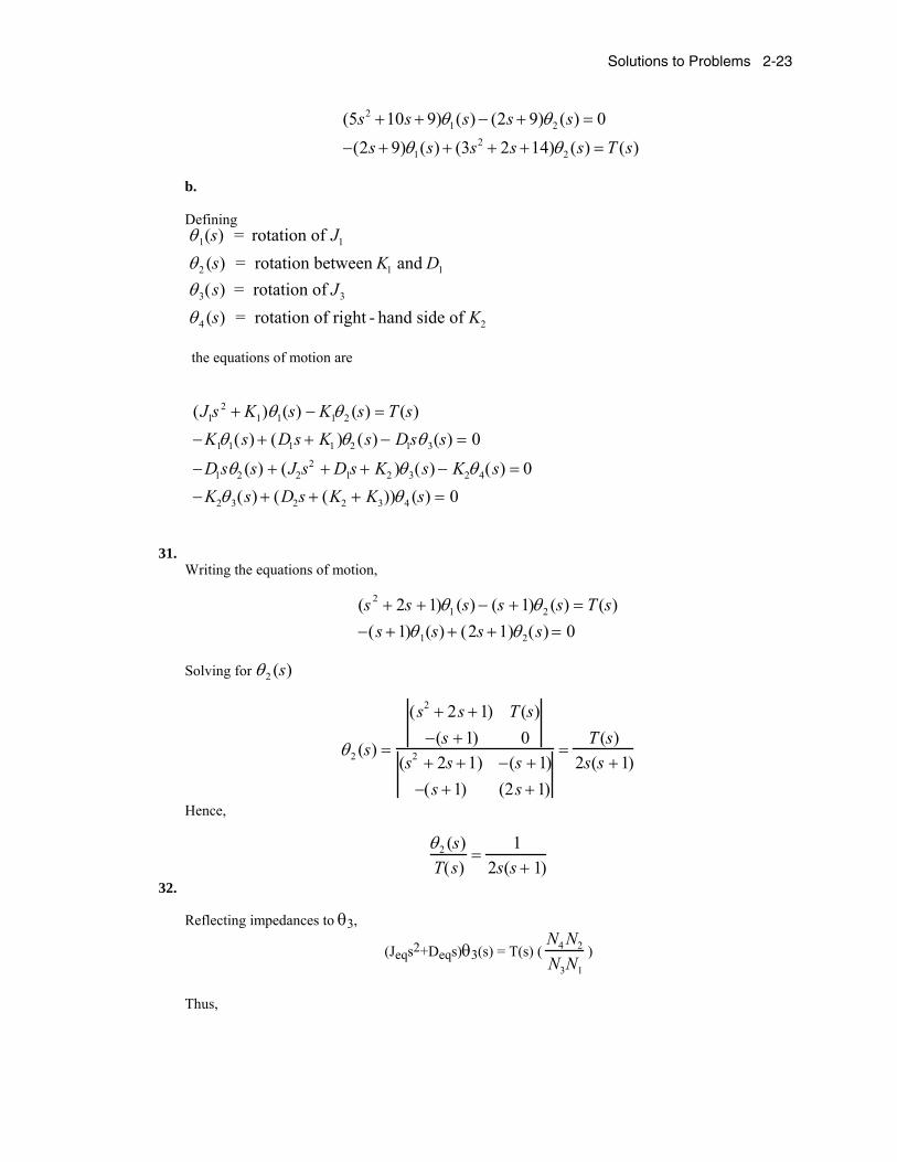
(J1s
2 + K1)θ1(s) − K1θ2 (s) = T (s)−K1θ1(s) + (D1s + K1 )θ2 (s) − D1sθ3(s) = 0
−D1sθ2 (s) + (J2s2 + D1s + K2 )θ3(s) − K2θ4(s) = 0
−K2θ3(s) + (D2s + (K2 + K3))θ4 (s) = 0
31.
Writing the equations of motion,
(s 2 + 2s +1)θ1 (s) − (s +1)θ2 (s) = T (s)−(s +1)θ1(s) + (2s +1)θ2(s) = 0
Solving for θ2 (s)
θ2 (s) =
(s2 + 2s +1) T (s)−(s +1) 0
(s2 + 2s +1) −(s +1)−(s +1) (2s +1)
=T (s)
2s(s +1)
Hence,
θ2 (s)T(s)
=1
2s(s + 1)
32.
Reflecting impedances to θ3,
(Jeqs2+Deqs)θ3(s) = T(s) (N4 N2
N3N1
)
Thus,
2-24 Chapter 2: Modeling in the Frequency Domain
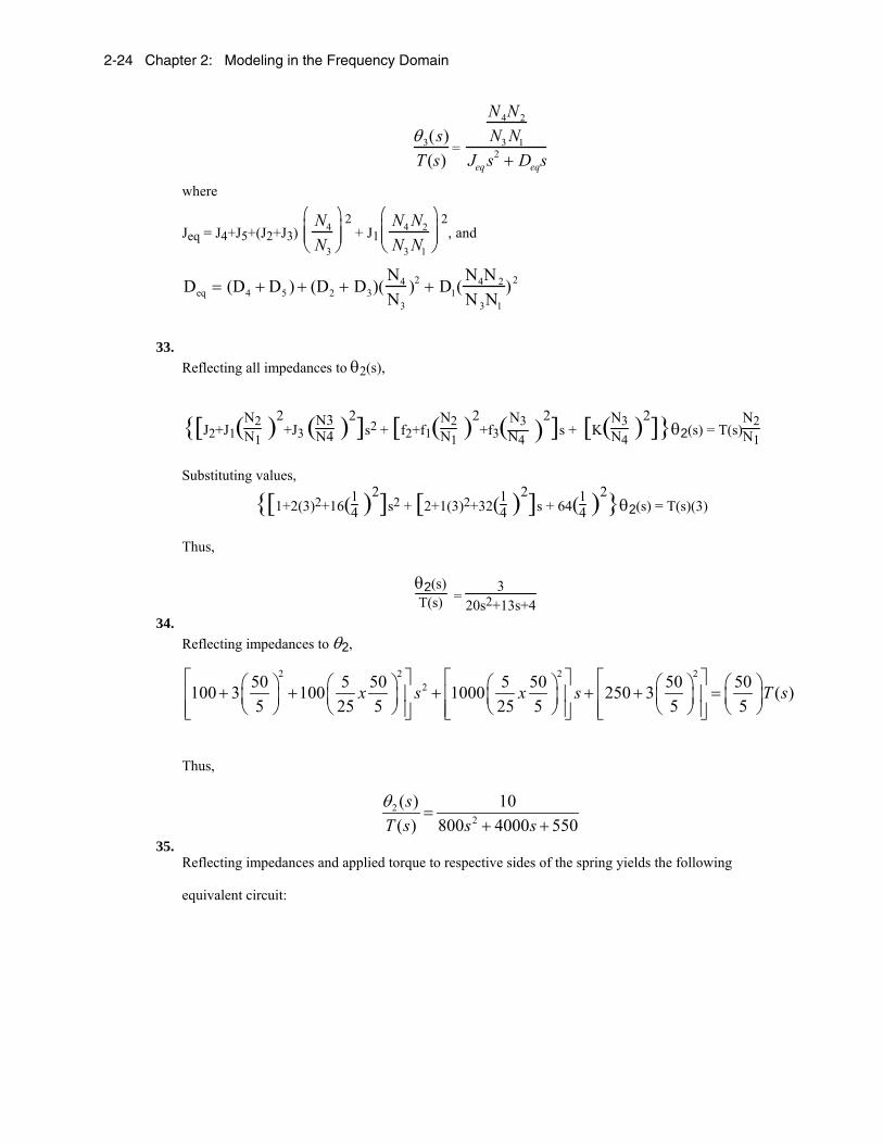
θ3(s)T (s)
=
N4N2
N3 N1
Jeq s2 + Deqs
where
Jeq = J4+J5+(J2+J3) N4
N3
⎛
⎝ ⎜ ⎜
⎞
⎠ ⎟ ⎟
2 + J1
N4 N2
N3 N1
⎛
⎝ ⎜ ⎜
⎞
⎠ ⎟ ⎟
2, and
Deq = (D4 + D5 ) + (D2 + D3)(N4
N3
)2 + D1(N4N 2
N 3N1
)2
33. Reflecting all impedances to θ2(s),
[J2+J1(N2
N1 )2
+J3 (N3N4 )
2]s2 + [f2+f1(N2N1
)2+f3(N3
N4 )
2]s + [K(N3N4
)2]θ2(s) = T(s)N2N1
Substituting values,
[1+2(3)2+16(14 )2]s2 + [2+1(3)2+32(1
4 )2]s + 64(14 )2θ2(s) = T(s)(3)
Thus,
θ2(s)T(s) =
320s2+13s+4
34. Reflecting impedances to θ2,
2 2 2 2250 5 50 5 50 50 50100 3 100 1000 250 3 ( )
5 25 5 25 5 5 5x s x s T s
⎡ ⎤ ⎡ ⎤ ⎡ ⎤⎛ ⎞ ⎛ ⎞ ⎛ ⎞ ⎛ ⎞ ⎛ ⎞+ + + + + =⎢ ⎥ ⎢ ⎥ ⎢ ⎥⎜ ⎟ ⎜ ⎟ ⎜ ⎟ ⎜ ⎟ ⎜ ⎟⎝ ⎠ ⎝ ⎠ ⎝ ⎠ ⎝ ⎠ ⎝ ⎠⎢ ⎥ ⎢ ⎥ ⎢ ⎥⎣ ⎦ ⎣ ⎦ ⎣ ⎦
Thus,
22
( ) 10( ) 800 4000 550s
T s s sθ
=+ +
35.
Reflecting impedances and applied torque to respective sides of the spring yields the following equivalent circuit:

Solutions to Problems 2-25
Writing the equations of motion,
2θ2(s) -2 θ3(s) = 2.6923T(s)
–2θ2(s) + (0.551s+2)θ3(s) = 0
Solving for θ3(s),
( )
3
2 2.6923 ( )2 0 5.3846 ( ) 4.8862 ( )( )
2 2 1.1022 0.551 2
T sT s T sss s
s
θ−
= = =−
− +
Hence, 3 ( ) 4.8862( )s
T s sθ
= . But, 4 3( ) 0.192 ( )s sθ θ= . Thus, 4 ( ) 0.938( )s
T s sθ
= .
36. Reflecting impedances and applied torque to respective sides of the viscous damper yields the following equivalent circuit:
Writing the equations of motion,
22 3
2 3 4
3 4
(2 2 ) ( ) 2 ( ) 3 ( )2 ( ) (2 5) ( ) 5 ( ) 05 ( ) (2 5) ( ) 0
s s s s s T ss s s s s
s s s
θ θθ θ θ
θ θ
+ − =− + + − =− + + =
Solving for θ4 (s) ,
2 0.955

2-26 Chapter 2: Modeling in the Frequency Domain
4 2
2 ( 1) 2 3 ( )2 (2 5) 00 5 0 30 ( )( )
2 ( 1) 2 0 (8 40 20)2 (2 5) 50 5 (2 5)
s s s T ss s
T sss s s s s s
s ss
θ
+ −− +
−= =
+ − + +− + −
− +
But, θ L(s) = 5θ4 (s) . Hence,
( )4
2 2
( ) 150 37.5( ) (8 40 20) 2 10 5s
T s s s s s s sθ
= =+ + + +
37. Reflect all impedances on the right to the viscous damper and reflect all impedances and torques on the
left to the spring and obtain the following equivalent circuit:
Writing the equations of motion,
(J1eqs2+K)θ2(s) -Kθ3(s) = Teq(s)
-Kθ2(s)+(Ds+K)θ3(s) -Dsθ4(s) = 0
-Dsθ3(s) +[J2eqs2 +(D+Deq)s]θ4(s) = 0
where: J1eq = J2+(Ja+J1)(N2N1
)2 ; J2eq = J3+(JL+J4)(N3
N4 )2
; Deq = DL(N3N4
)2 ; θ2(s) = θ1(s)
N1N2
.

Solutions to Problems 2-27
38. Reflect impedances to the left of J5 to J5 and obtain the following equivalent circuit:
Writing the equations of motion,
[Jeqs2+(Deq+D)s+(K2+Keq)]θ5(s) -[Ds+K2]θ6(s) = 0
-[K2+Ds]θ5(s) + [J6s2+2Ds+K2]θ6(s) = T(s)
From the first equation, θ6(s)θ5(s)
= Jeqs2+(Deq+D)s+ (K2+Keq)
Ds+K2 . But,
θ5(s)θ1(s)
= N1N3N2N4
. Therefore,
θ6(s)θ1(s)
= N1N3N2N4
⎝⎜⎛
⎠⎟⎞
Jeqs2+(Deq+D)s+ (K2+Keq)
Ds+K2 ,
where Jeq = [J1(N4N2N3N1
)2 + (J2+J3)(N4
N3 )2
+ (J4+J5)], Keq = K1(N4N3
)2 , and
Deq = D[(N4N2N3N1
)2 + (N4
N3 )2
+ 1].
39. Draw the freebody diagrams,

2-28 Chapter 2: Modeling in the Frequency Domain
Write the equations of motion from the translational and rotational freebody diagrams,
(Ms2+2fv s+K2)X(s) -fvrsθ(s) = F(s)
-fvrsX(s) +(Js2+fvr2s)θ(s) = 0
Solve for θ(s),
θ(s) =
Ms2+2fvs+K2
F(s)
-fvrs 0
Ms2+2fvs+K2
-fvrs
-fvrs Js2+fvr2s
= fvrF(s)
JMs3+(2Jfv+Mfvr2)s2+(JK
2+fv
2r2)s+K
2fvr2
From which, θ(s)F(s) =
fvrJMs3+(2Jfv+Mfvr2)s2+(JK2+fv2r2)s+K2fvr2
.
40.
Draw a freebody diagram of the translational system and the rotating member connected to the
translational system.
From the freebody diagram of the mass, F(s) = (2s2+2s+3)X(s). Summing torques on the rotating
member,
(Jeqs2 +Deqs)θ(s) + F(s)2 = Teq(s). Substituting F(s) above, (Jeqs2 +Deqs)θ(s) + (4s2+4s+6)X(s) =
Teq(s). However, θ(s) = X(s)
2 . Substituting and simplifying,
Teq = [(Jeq2 +4)s2 +(Deq
2 +4)s+6]X(s)
22 3

Solutions to Problems 2-29
But, Jeq = 3+3(4)2 = 51, Deq = 1(2)2 +1 = 5, and Teq(s) = 4T(s). Therefore,
[ 592
s2 +132
s+6]X(s) = 4T(s). Finally, X(s)T(s) = 2
859 13 12s s+ +
.
41. Writing the equations of motion,
(J1s2+K1)θ1(s) - K1θ2(s) = T(s) -K1θ1(s) + (J2s2+D3s+K1)θ2(s) +F(s)r -D3sθ3(s) = 0 -D3sθ2(s) + (J2s2+D3s)θ3(s) = 0
where F(s) is the opposing force on J2 due to the translational member and r is the radius of J2. But,
for the translational member,
F(s) = (Ms2+fvs+K2)X(s) = (Ms2+fvs+K2)rθ(s)
Substituting F(s) back into the second equation of motion,
(J1s2+K1)θ1(s) - K1θ2(s) = T(s)
-K1θ1(s) + [(J2 + Mr2)s2+(D3 + fvr2)s+(K1 + K2r2)]θ2(s) -D3sθ3(s) = 0
-D3sθ2(s) + (J2s2+D3s)θ3(s) = 0 Notice that the translational components were reflected as equivalent rotational components by the
square of the radius. Solving for θ2(s), θ2 (s) =K1(J3s
2 + D3s)T(s)∆
, where ∆ is the
determinant formed from the coefficients of the three equations of motion. Hence,
θ2 (s)T(s)
=K1(J3s
2 + D3s)∆
Since
X(s) = rθ2 (s), X(s)T (s)
=rK1(J3s
2 + D3s)∆
42. Kt
Ra
= Tstall
Ea
= 20050
= 4 ; Kb = Ea
ωno− load
= 50300
= 16
Also,
Jm = 10+18( 13)2
= 12; Dm = 8+36( 13)2
= 12.
Thus, θm (s)Ea (s)
= 4 /121 4( (12 ))
12 6s s + +
= 1/ 3
19( )18
s s +
Since θL(s) = 13
θm(s),

2-30 Chapter 2: Modeling in the Frequency Domain
θL(s)Ea (s)
=
19
19( )18
s s +
43. The parameters are:
Kt
Ra
= Ts
Ea
= 55
= 1; Kb = Ea
ω=
5600π
2π 160
=
14
; Jm =1614
⎛ ⎝
⎞ ⎠
2
+ 412
⎛ ⎝
⎞ ⎠
2
+1 = 3; Dm = 3214
⎛ ⎝
⎞ ⎠
2
= 2
Thus,
θm (s)Ea (s)
=
13
s(s + 13
(2 + (1)(14
)))=
13
s(s + 0.75)
Since θ2(s) = 14
θm(s),
θ2 (s)Ea (s)
=
112
s(s + 0.75).
44. The following torque-speed curve can be drawn from the data given:
v
T
100
50
500 1000
Therefore, Kt
Ra
= Tstall
Ea
= 10012
; Kb = Ea
ωno− load
= 12
1333.33. Also, Jm = 7+105( 1
6)2
= 9.92; Dm =
3. Thus,
θm (s)Ea (s)
=
100 112 9.92
1( (3.075))9.92
s s
⎛ ⎞⎜ ⎟⎝ ⎠
+=
0.84( 0.31)s s +
. Since θL(s) = 16
θm(s), θL(s)Ea (s)
= 0.14
( 0.31)s s +.
45.
55
600 1333.33
Solutions to Problems 2-31
From Eqs. (2.45) and (2.46),
RaIa(s) + Kbsθ(s) = Ea(s) (1)
Also,
Tm(s) = KtIa(s) = (Jms2+Dms)θ(s). Solving for θ(s) and substituting into Eq. (1), and simplifying
yields
Ia (s)Ea (s)
= 1Ra
(s +Dm
Jm
)
s + Ra Dm + KbKt
RaJm
(2)
Using Tm(s) = KtIa(s) in Eq. (2),
Tm(s)Ea (s)
= Kt
Ra
(s +Dm
Jm
)
s + Ra Dm + KbKt
RaJm
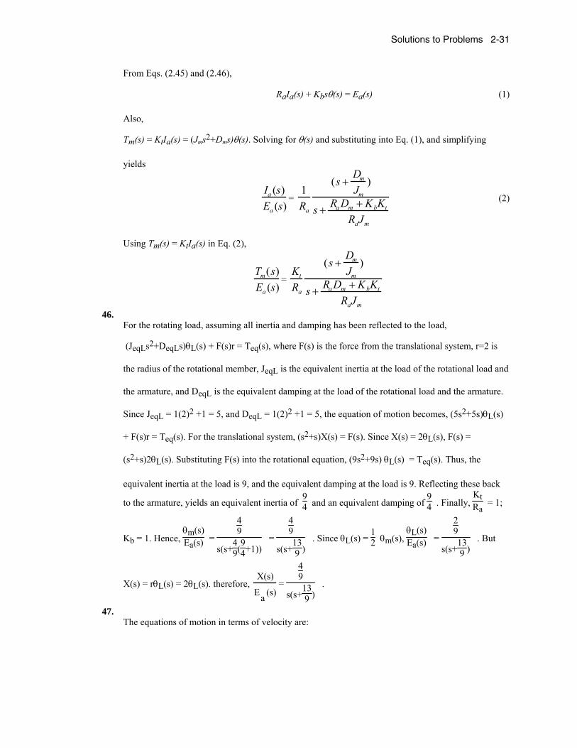
46. For the rotating load, assuming all inertia and damping has been reflected to the load,
(JeqLs2+DeqLs)θL(s) + F(s)r = Teq(s), where F(s) is the force from the translational system, r=2 is
the radius of the rotational member, JeqL is the equivalent inertia at the load of the rotational load and
the armature, and DeqL is the equivalent damping at the load of the rotational load and the armature.
Since JeqL = 1(2)2 +1 = 5, and DeqL = 1(2)2 +1 = 5, the equation of motion becomes, (5s2+5s)θL(s)
+ F(s)r = Teq(s). For the translational system, (s2+s)X(s) = F(s). Since X(s) = 2θL(s), F(s) =
(s2+s)2θL(s). Substituting F(s) into the rotational equation, (9s2+9s) θL(s) = Teq(s). Thus, the
equivalent inertia at the load is 9, and the equivalent damping at the load is 9. Reflecting these back
to the armature, yields an equivalent inertia of 94 and an equivalent damping of
94 . Finally,
KtRa
= 1;
Kb = 1. Hence, θm(s)Ea(s) =
49
s(s+49(
94+1))
=
49
s(s+139 )
. Since θL(s) = 12 θm(s),
θL(s)Ea(s) =
29
s(s+139 )
. But
X(s) = rθL(s) = 2θL(s). therefore, X(s)
Ea (s)=
49
s(s+139 )
.
47. The equations of motion in terms of velocity are:

2-32 Chapter 2: Modeling in the Frequency Domain
[M1s + ( fv1 + fv 3) + K1
s+ K2
s]V1(s) − K2
sV2(s) − fv 3V3(s) = 0
−K2
sV1(s) + [M2s + ( fv 2 + fv 4) +
K2
s]V2 (s) − fv4V3 (s) = F(s)
− fv3V1 (s) − fv4V2 (s) + [M3s + fV3 + fv4]V3(S) = 0
For the series analogy, treating the equations of motion as mesh equations yields
In the circuit, resistors are in ohms, capacitors are in farads, and inductors are in henries. For the parallel analogy, treating the equations of motion as nodal equations yields
In the circuit, resistors are in ohms, capacitors are in farads, and inductors are in henries.
48. Writing the equations of motion in terms of angular velocity, Ω(s) yields
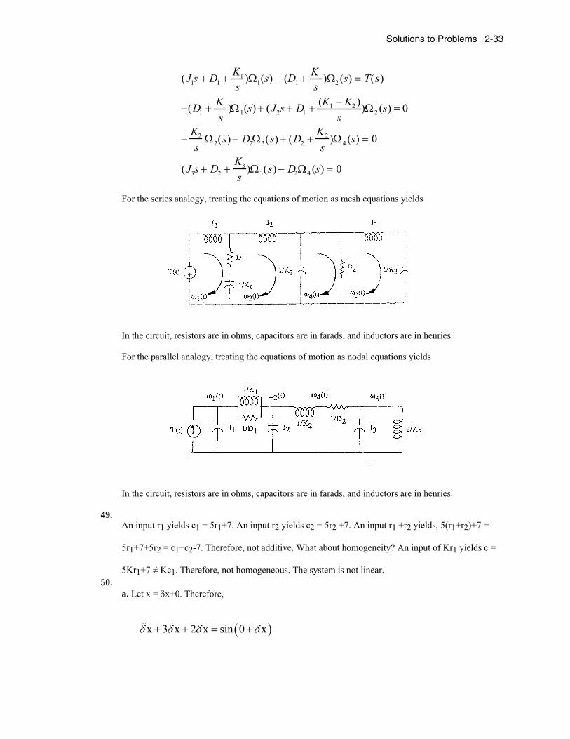
Solutions to Problems 2-33
(J1s + D1 + K1
s)Ω1(s) − (D1 + K1
s)Ω2 (s) = T(s)
−(D1 + K1
s)Ω1(s) + (J2s + D1 + (K1 + K2 )
s)Ω2 (s) = 0
−K2
sΩ2(s) − D2Ω3(s) + (D2 +
K2
s)Ω4 (s) = 0
(J3s + D2 +K3
s)Ω3(s) − D2Ω4 (s) = 0
For the series analogy, treating the equations of motion as mesh equations yields
In the circuit, resistors are in ohms, capacitors are in farads, and inductors are in henries. For the parallel analogy, treating the equations of motion as nodal equations yields
In the circuit, resistors are in ohms, capacitors are in farads, and inductors are in henries.
49.
An input r1 yields c1 = 5r1+7. An input r2 yields c2 = 5r2 +7. An input r1 +r2 yields, 5(r1+r2)+7 =
5r1+7+5r2 = c1+c2-7. Therefore, not additive. What about homogeneity? An input of Kr1 yields c =
5Kr1+7 ≠ Kc1. Therefore, not homogeneous. The system is not linear. 50.
a. Let x = δx+0. Therefore,
( )x 3 x 2 x sin 0 xδ δ δ δ+ + = +
2-34 Chapter 2: Modeling in the Frequency Domain
( )x 0 x 0
d sin xBut,sin 0 x sin 0 | x 0 cos x | x xdx
δ δ δ δ= =
+ = + = + =
Therefore, 5 3x x x xδ δ δ δ+ + = . Collecting terms, 5 2 0x x xδ δ δ+ + = .
b. Let x = δx+π. Therefore,
( )x 3 x 2 x sin xδ δ δ π δ+ + = +
( )x x
d sin xBut,sin x sin | x 0 cos x | x xdx π π
π δ π δ δ δ= =
+ = + = + = −
Therefore, x 5 x 3 x xδ δ δ δ+ + = − . Collecting terms, x 5 x 2 x 0δ δ δ+ + = .
51.
If x = 0 + δx, ( )xx 10 x 31 x 30 x e δδ δ δ δ −+ + + =
( )x
x 0 x
x 0 x 0
deBut,e e | x 1 e | x 1 xdx
δ δ δ δ−
− − −
= == + = − = −
Therefore, x 10 x 31 x 30 x 1 xδ δ δ δ δ+ + + = − , or, x 10 x 31 x 31 x 1δ δ δ δ+ + + = . 52.
The given curve can be described as follows:
f(x) = –5 ; –∞<x<–1;
f(x) = 5x; –1<x<1;
f(x) = 5; 1<x<+∞
Thus, a . 17 50 5b. 17 50 5 or 17 45 0c. 17 50 5
x x xx x x x x x xx x x
+ + = −+ + = + + =+ + =
53. The relationship between the nonlinear spring’s displacement, xs(t) and its force, fs(t) is
xs ( t) = 1 − e− fs ( t)
Solving for the force,
fs (t) = − ln(1 − xs (t)) (1)
Writing the differential equation for the system by summing forces,
d2 x(t)dt2 +
dx(t)dt
− ln(1− x(t)) = f (t) (2)
Letting x(t) = x0 + δx and f(t) = 1 + δf, linearize ln(1 – x(t)).
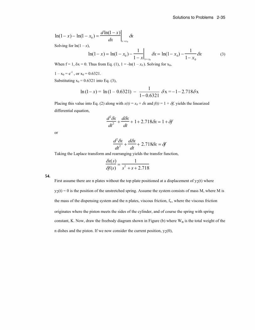
Solutions to Problems 2-35
ln(1− x) − ln(1 − x0 ) =d ln(1 − x)
dx x =x 0
δx
Solving for ln(1 – x),
ln(1− x) = ln(1 − x0 ) −1
1 − x x= x0
δx = ln(1− x0) −1
1− x0
δx (3)
When f = 1, δx = 0. Thus from Eq. (1), 1 = -ln(1 – x0 ). Solving for x0, 1 – x0 = e-1 , or x0 = 0.6321.
Substituting x0 = 0.6321 into Eq. (3),
1ln (1 ) = ln (1 – 0.6321) x = 1 2.718 x1 0.6321
x δ δ− − − −−
Placing this value into Eq. (2) along with x(t) = x0 + δx and f(t) = 1 + δf, yields the linearized
differential equation,
d2δxdt2 +
dδxdt
+ 1+ 2.718δx = 1 +δf
or
d2δxdt2 +
dδxdt
+ 2.718δx = δf
Taking the Laplace transform and rearranging yields the transfer function,
δx(s)δf (s)
=1
s2 + s + 2.718
54. First assume there are n plates without the top plate positioned at a displacement of y2(t) where
y2(t) = 0 is the position of the unstretched spring. Assume the system consists of mass M, where M is
the mass of the dispensing system and the n plates, viscous friction, fv, where the viscous friction
originates where the piston meets the sides of the cylinder, and of course the spring with spring
constant, K. Now, draw the freebody diagram shown in Figure (b) where Wn is the total weight of the
n dishes and the piston. If we now consider the current position, y2(0),
2-36 Chapter 2: Modeling in the Frequency Domain
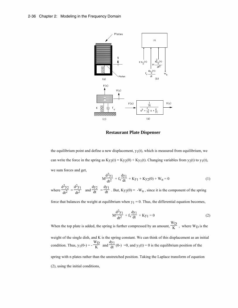
Restaurant Plate Dispenser
the equilibrium point and define a new displacement, y1(t), which is measured from equilibrium, we
can write the force in the spring as Ky2(t) = Ky2(0) + Ky1(t). Changing variables from y2(t) to y1(t),
we sum forces and get,
Md2y1dt2
+ fvdy1dt + Ky1 + Ky2(0) + Wn = 0 (1)
where d2y2dt2
= d2y1dt2
and dy2dt =
dy1dt . But, Ky2(0) = -Wn , since it is the component of the spring
force that balances the weight at equilibrium when y1 = 0. Thus, the differential equation becomes,
Md2y1dt2
+ fvdy1dt + Ky1 = 0 (2)
When the top plate is added, the spring is further compressed by an amount, WDK , where WD is the
weight of the single dish, and K is the spring constant. We can think of this displacement as an initial
condition. Thus, y1(0-) = - WDK and
dy1dt (0-) =0, and y1(t) = 0 is the equilibrium position of the
spring with n plates rather than the unstretched position. Taking the Laplace transform of equation
(2), using the initial conditions,
Solutions to Problems 2-37
M(s2Y1(s) + sWDK ) + fv(sY1(s) +
WDK ) + KY1(s) = 0 (3)
or
(Ms2 + fvs + K)Y1(s) = -WD
K(Ms + fv ) (4)
Now define a new position reference, Y(s), which is zero when the spring is compressed with the
initial condition,
Y(s) = Y1(s) + WDKs (5)
or
Y1(s) = Y(s) - WDKs (6)
Substituting Y1(s) in Equation (4), we obtain,
(Ms2 + fvs + K)Y(s) = WD
s = F(s) (7)
a differential equation that has an input and zero initial conditions. The schematic is shown in Figure
(c). Forming the transfer function, Y(s)F(s) , we show the final result in Figure (d), where for the
removal of the top plate, F(s) is always a step, F(s) = WD
s .
55.
We have ψφφφ )(aJkbJ =++
Assuming zero initial conditions and obtaining Laplace transform on both sides of the equation we
obtain:
)()()()()(2 saJsksbssJs Ψ=Φ+Φ+Φ
From which we get:
kbsJsaJ
ss
++=
ΨΦ
2)()(
56.
a. We choose Laplace transforms to obtain a solution. After substitution of numerical values the
equations become:
)(7.0)(9.0)( tNtCdt
tdC+−=
)()(02.0)(1.0)( tItNtCdt
tdN+−−=

2-38 Chapter 2: Modeling in the Frequency Domain
Obtaining Laplace transforms and substituting initial values we obtain:
)(7.0)(9.047000500)( sNsCssC +−=−
)()(02.0)(1.061100500)( sIsNsCssN +−−=−
Both equations are manipulated as follows:
9.047000500
9.0)(7.0)(
++
+=
sssNsC
02.0)(
02.061100500
02.0)(1.0)(
++
++
+−
=s
sIss
sCsN
Substituting the first equation into the second one gets:
)9.0)(02.0(088.092.0
02.0)(
02.061100500
)9.0)(02.0(4700050
)9.0)(02.0(07.01
02.0)(
02.061100500
)9.0)(02.0(4700050
)( 2
++++
++
++
++−
=
+++
++
++
++−
=
ssss
ssI
sss
ss
ssI
ssssN
088.092.04700050
088.092.0)9.0(61100500)(
088.092.09.0
222 ++−
+++
+++
+=
ssssssI
sss
From which we get the block diagram:
088.092.0)9.0(
2 +++
sssI(s)
61100500
9.04700050
+s
+
+-
b. Letting s
sI6106)( ×
= and after algebraic manipulations one gets:
)1084.0)(8116.0(10545629040061100500
)088.092.0(10545629040061100500)(
52
2
52
++×++
=++
×++=
sssss
ssssssN
1084.0103.19
8116.0107101354.6
1084.08116.0
447
+×
−+
×−
×=
++
++=
ssssC
sB
sA
Solutions to Problems 2-39
Obtaining the inverse Laplace transform: tt eetN 1084.048116.047 103.19107101364.6)( −− ×−×−×=
57.
a.
‘Exact’:
From Figure (a)
( ) ( )0.0050.005
1 1 2 12 18 8 8( ) ( )1 1 18 8 8
ss
o in
eeV s V s
ss s s s
−− −−= = =
⎛ ⎞+ + +⎜ ⎟⎝ ⎠
Using Partial fraction expansions note that 1
11)1(
1+
−=+ ssss
. Thus, applying partial fraction
expansion to Vo(s) and taking the inverse Laplace transform yields,
So 1 1( 0.005)8 8( ) 2(1 ) ( ) 2(1 ) ( 0.005)
t t
ov t e u t e u t− − −
= − − − −
‘Impulse’: 1 1
0.001258 8( ) ( ) 0.011 1 0.1258 8
o inV s V sss s
= = =++ +
In this case 0.125( ) 0.00125 tov t e−=
b.
The following M-File will simulate both inputs: syms s s = tf('s'); G=(1/8)/(s+(1/8)); t=0:1e-4:10; for i=1:max(size(t)), if(i*1e-4 <= 5e-3) vinexact(i) = 2; else vinexact(i) = 0; end end yexact = lsim(G,vinexact,t); yimpulse = 0.00125*exp(-(1/8)*t); plot(t,yexact,t,yimpulse)

2-40 Chapter 2: Modeling in the Frequency Domain
Resulting in the following figure:
Both outputs are indistinguishable at this scale. However zooming closer to t=0 will show
differences.
58. a. At equilibrium
02
2
=dt
Hd. From which we get that 2
2
HIkmg = or
mgkIH 00 =
b. Following the ‘hint’ procedure:
IHH
HHIIkH
HHHHII
kdt
Hdm IHIH δδ
δδδ
δδδδ
δδδδ 0,040
200
0,040
02
02
2
)()()(2
)()()(2
==== +++
−+
++=
After some algebraic manipulations this becomes:
ImH
kIH
mHkI
dtHdm δδδ
20
030
20
2
2 22−=
Obtaining Laplace transform on both sides of the equation one obtains the transfer function:

Solutions to Problems 2-41
30
202
20
0
2
2
)()(
mHkI
s
mHkI
sIsH
−−=
δδ
59.
The two differential equations for this system are:
0)()( =−+−+ wsawsasb xxCxxKxM
0)()()( =−+−+−+ rxKxxCxxKxM wtswaswawus
Obtaining Laplace transform on both sides gives
0)()( 2 =+−++ waasaab XsCKXKsCsM
tsaawtaaus RKXsCKXKKsCsM =+−+++ )())(( 2
Solving the first equation for sX and substituting into the second one gets
( ) 222
2
)()()()()(
sCKKsCsMKKsCsMKsCsMKs
RX
aaaabtaaus
aabtw
+−+++++++
=
60. a. The three equations are transformed into the Laplace domain:
SkCKkSSs S ψψ −=− ~0
)~( CKSkCs M−= ψ
CkPs 2=
The three equations are algebraically manipulated to give:
Cks
Kkks
SS S
ψ
ψ
ψ ++
+=
~0
MKksSk
C ~ψ
ψ
+=
Cs
kP 2=
By direct substitutions it is obtained that:
2-42 Chapter 2: Modeling in the Frequency Domain
022 )~~()~1()~(
SKKksKks
KksS
SMM
M
−+++
+=
ψψ
ψ
022 ))~~()~1((S
KKksKksk
CSMM −+++
=ψψ
ψ
0222
))~~()~1((S
KKksKksskk
PSMM −+++
=ψψ
ψ
b. 0)()(
0==∞
→ssSLimS
s
0)()(0
==∞→
ssCLimCs
02
022
02
0)~~()~~(
)()( SK
kkKk
SkKKk
SkkssPLimP
SSSM
s=
−+=
−==∞
→
ψψ
ψ
ψ
61.
Eliminate balT by direct substitution. This results in
)()()()(0
2
2
tTdttJtJtkJdtdJ d
t
+−−−= ∫θρθηθθ
Obtaining Laplace transform on both sides of this equation and eliminating terms one gets that:
ρη +++=
Θksss
sJs
Td23
1
)(
62.
a.
We have that
φgmxm LLaL =
LTLa xxx −=
φLxL =
From the second equation
φφ gLvxxx TLTLa =−=−=
Solutions to Problems 2-43
Obtaining Laplace transforms on both sides of the previous equation
Φ=Φ− gLssVT from which )( 2LsgsVT +Φ=
so that
20
22
2
11)(ω+
=+
=+
=Φ
ss
LLgs
sLLsg
ssVT
b. Under constant velocity s
VsVT
0)( = so the angle is
20
20 1)(
ω+=Φ
sLV
s
Obtaining inverse Laplace transform
)sin()( 00
0 tLV
t ωω
φ = , the load will sway with a frequency 0ω .
c. From φgmfxm LTTT −− and Laplace transformation we get
TLTTLTLTTT Xs
sL
gmFVs
sL
gmFsgmFsXsm 20
2
2
20
22 11)()(
ωω +−=
+−=Φ−=
From which
)(1
))(()1(
120
22
20
2
20
20
22
20
2
20
22 ω
ωωω
ω
ωass
smmsms
s
sLgmmsF
X
TLTLT
T
T
++
=++
+=
++
=
Where T
L
mma += 1
d. From part c
)(1
20
2
20
2
ωωass
smF
sXFV
TT
T
T
T
++
==
Let s
FFT
0= then
20
2220
22
20
20
)()(
ωωω
asDCs
sB
sA
asss
mF
sVT
T ++
++=++
=
After partial fraction expansions, so
)cos('')( 0 θω +++= taCBtAtvT
From which it is clear that ∞⎯⎯⎯ →⎯ ∞⎯→⎯tTv
2-44 Chapter 2: Modeling in the Frequency Domain
63.
a. Obtaining Laplace transforms on both sides of the equation
)()( 0 sKNNssN =− or Ks
NsN
−= 0)(
By inverse Laplace transformation KteNtN 0)( =
b. Want to find the time at which
00 2NeN Kt =
Obtaining ln on both sides of the equation
Kt 2ln
=
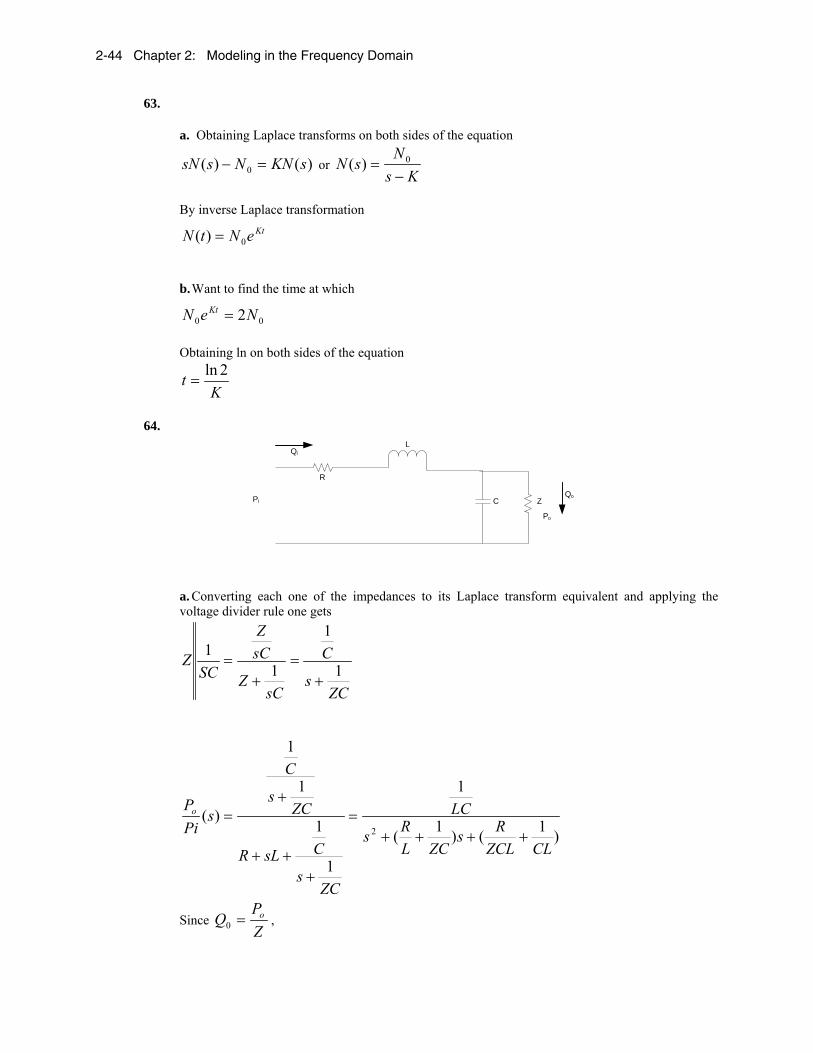
64.
R
C
L
ZPi
Qi
Qo
Po
a. Converting each one of the impedances to its Laplace transform equivalent and applying the voltage divider rule one gets
ZCs
C
sCZ
sCZ
SCZ
1
1
11
+=
+=
)1()1(
1
1
1
1
1
)(2
CLZCLRs
ZCLRs
LC
ZCs
CsLR
ZCs
C
sPiPo
++++=
+++
+=
Since ZP
Q o=0 ,

Solutions to Problems 2-45
9.73550125.330236.0
)1()1(
1
)( 22 ++
=++++
=ss
CLZCLRs
ZCLRs
LCZsPQ
i
o
b. The steady state circuit becomes
R
ZPi
Qi
Qo
Po
So that 60 102.3
30816341761 −=
+=
+= X
ZRP
Q i
c. Applying the final value theorem
6
20
102.319.73550125.33
0236.0)( −
⎯→⎯
=++
=∞ Xsss
sq Lims
o
65. The laplace transform of the systems output is
Dividing by the input one gets
66.
a. By direct differentiation )()()( )1(
0 tVeeeVdt
tdV tetat
ααλ
α λααλ −−− ==
−
b. αλ
αλ α
eVeVLimtVLimVte
tt0
)1(
0)()( ===∞−−
∞⎯→⎯∞⎯→⎯
c.
Lambda = 2.5;
alpha = 0.1;
V0=50;
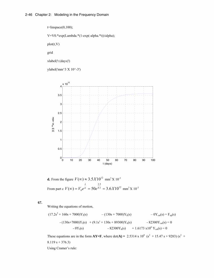
2-46 Chapter 2: Modeling in the Frequency Domain
t=linspace(0,100);
V=V0.*exp(Lambda.*(1-exp(-alpha.*t))/alpha);
plot(t,V)
grid
xlabel('t (days)')
ylabel('mm^3 X 10^-3')
0 10 20 30 40 50 60 70 80 90 1000
0.5
1
1.5
2
2.5
3
3.5
4x 10
12
t (days)
mm3 X 10-3
d. From the figure 12105.3)( XV ≈∞ mm3 X 10-3
From part c 121.05.2
0 106.350)( XeeVV ===∞ αλ
mm3 X 10-3
67.
Writing the equations of motion, (17.2s2 + 160s + 7000)Yf(s) – (130s + 7000)Yh(s) – 0Ycat(s) = Fup(s)
- (130s+7000)Yf(s) + (9.1ss + 130s + 89300)Yh(s) - 82300Ycat(s) = 0
- 0Yf(s) - 82300Yh(s) + 1.6173 x10⁶ Ycat(s) = 0 These equations are in the form AY=F, where det(A) = 2.5314 x 10⁸ (s2 + 15.47 s + 9283) (s2 +
8.119 s + 376.3)
Using Cramer’s rule:

Solutions to Problems 2-47
Ycat (s)Fup(s)
=0.04227(s + 53.85)
(s2 +15.47s + 9283)(s 2 + 8.119s + 376.3)
Yh(s)Fup(s)
=0.8306(s + 53.85)
(s2 +15.47s + 9283)(s2 + 8.119s + 376.3)
Yh(s) − Ycat (s)
Fup(s)=
0.7883(s + 53.85)(s2 + 15.47s + 9283)(s2 +8.119s + 376.3)
68. a. The first two equations are nonlinear because of the Tv products on their right hand side. Otherwise the equations are linear.
b. To find the equilibria let 0*
===dtdv
dtdT
dtdT
Leading to
0=−− νβTdTs
0* =− TTv µβ
0* =− cvkT
The first equilibrium is found by direct substitution. For the second equilibrium, solve the last two
equations for T*
µβTvT =*
and kcvT =* . Equating we get that
kcTβµ
=
Substituting the latter into the first equation after some algebraic manipulations we get that
βµd
cksv −= . It follows that
βµ kcds
kcvT −==* .
69.
a. From mkFFa
m
w
•
−= , we have: amkFFFamkFF mStLRmw O •••• ++++=+= (1)
Substituting for the motive force, F, and the resistances FRo, FL, and Fst using the equations given
in the problem, yields the equation:
2-48 Chapter 2: Modeling in the Frequency Domain
amkvvACgmgmfv
PF mhwwtot••⎟
⎠⎞⎜
⎝⎛•••••••••
•++++== 25.0sincos ρααη
(2)
b. Noting that constant acceleration is assumed, the average values for speed and acceleration are:
aav = 20 (km/h)/ 4 s = 5 km/h.s = 5x1000/3600 m/s2 = 1.389 m/s2
vav = 50 km/h = 50,000/3,600 m/s = 13.89 m/s
The motive force, F (in N), and power, P (in kW) can be found from eq. 2:
Fav = 0.011 x 1590 x 9.8 + 0.5 x 1.2 x 0.3 x 2 x 13.892 + 1.2 x 1590 x 1.389 = 2891 N
Pav = Fav. v / η tot = 2891 x 13.89 / 0.9 = 44, 617 N.m/s = 44.62 kW
To maintain a speed of 60 km/h while climbing a hill with a gradient α = 5o, the car engine or
motor needs to overcome the climbing resistance:
13585sin8.91590sin == ••••= αgmFSt N
Thus, the additional power, Padd, the car needs after reaching 60 km/h to maintain its speed while
climbing a hill with a gradient α = 5o is:
η/vStFaddP •= = 1358 x 60 x 1000/(3,600 x 0.9) = 25, 149 W = 25.15 kW
c. Substituting for the car parameters into equation 2 yields:
dtdvvF / 1590 x 1.2 2 x 0.3 x 1.2 x 0.5 9.8 x 1590 x 0.011 2 ++=
or dtdvvtF / 1908 0.364.171)( 2 ++= (3)
To linearize this equation about vo = 50 km/h = 13.89 m/s, we use the truncated taylor series:
)2)2
22 (()(ooo
vv
o vvvvvdvvdvv
o
−−≈− •=
=
(4), from which we obtain:
2222 89.1378.27 −=− ••= vvvvv oo (5)

Solutions to Problems 2-49
Substituting from equation (5) into (3) yields:
dtdvvtF / 190846.69 014.171)( +−+= or
dtdvvtFFFtFtF oRoe / 1908 0146.694.171)()()( +=+−=+−= (6)
Equation (6) may be represented by the following block-diagram:
d. Taking the Laplace transform of the left and right-hand sides of equation (6) gives,
(s) 1908(s) 01)( sVVsFe += (7)
Thus the transfer function, Gv(s), relating car speed, V(s) to the excess motive force, Fe(s), when the
car travels on a level road at speeds around vo = 50 km/h = 13.89 m/s under windless conditions is:
sFVsGv 1908 01
1(s)(s))(
e +== (8)
Car Speed, v(t)
Gv
+
Fo = 69.46 N
+ Motive Force,
F (t)
Excess Motive Force, Fe(t)
FRo = 171.4 N