Modeling Money Demand under the Profit-Sharing Banking Scheme: Evidence on Policy Invariance and Long-Run Stability*

Amir Kia

(main contact) Department of Economics

Carleton University Ottawa, Ontario K1S 5B6 Canada

and

Ali F. Darrat

Department of Economics and Finance Louisiana Tech University

Ruston, LA 71272, USA

________________________________________________________________________ Abstract This paper extends the literature on interest-free banking systems by modeling money demand equations for Iran which has followed the profit-sharing scheme since the mid-1980s. Using quarterly data spanning the period 1966-2001, we estimate two alternative demand equations for M1 and profit-sharing deposits. Unlike prior research, this paper focuses on whether the estimated equations are policy invariant in addition of being temporally stable in the short- and long-run. Our empirical results persistently suggest that the two money demand models, and especially the demand for profit-sharing deposits, are structurally stable and policy invariant despite the numerous shocks that have characterized Iran in recent years. These results provide another piece of evidence supportive of the merit of the interest-free banking system, and suggest that profit-sharing monetary aggregates represent a credible instrument for monetary policy-making in Iran. Keywords: Interest-free banking system, Profit-sharing deposits, Policy-invariance,

Super-exogeneity, Long- run stability, Central Bank of Iran JEL Codes: E41, E52 ________________________________________________________________________ *Preliminary draft (prepared in Word 97) for presentation to ERF’s 10th Annual Conference to be held in Marrakech, Morocco, December 16-18, 2003. Not to be quoted without written permission from the authors. Amir Kia’s phone: (613) 520-2600, ext. 3753, fax: (613) 747-1352, e-mail: akia@ccs.carleton.ca. Ali F. Darrat’s phone and fax: (318) 257-3874, e-mail: darrat@cab.latech.edu. We wish to thank Mahmood Khataie for useful comments on an earlier draft and Sohrab Abizadeh for help with data. The usual disclaimer applies.

Modeling Money Demand under the Profit-Sharing Banking Scheme: Evidence on Policy Invariance and Long-Run Stability*

1. Introduction

The Islamic concept of profit-sharing, as opposed to the alternative more common

concept of predetermined (fixed) interest rates, has gained a great deal of popularity since the early 1980s. Recent data reveal that there are at least 180 Islamic banks and some 120 Islamic non-bank financial institutions operating in different parts of the world, with total assets approaching $200 billion and whose core business is fast growing at an annual rate of about 10 percent in recent years [Hassoune (2002)]. While most of these Islamic financial institutions exist in Muslim countries, many of these institutions operate in countries like Australia, Canada, France, Germany, Switzerland, the United Kingdom, and the United States. Moreover, major traditional banks like the Citibank have begun offering interest-free financial services to their clients.

Such remarkable growth and popularity of Islamic banks has also witnessed an

equally impressive volume of research on the nature and structure of these banks and on their efficiency relative to the more traditional interest-based banks1 However, with a few exceptions, all prior research on the merit of Islamic banks is essentially theoretical, void of any empirical substantiation of the issues involved. Among the notable exceptions are Darrat (1988) who examines the case of Islamic banking using data from Tunisia, Yousefi et al. (1997) and Darrat (2000) who study the experience of Iran, and more recently Darrat (2002) on the case of Islamic banking in Iran and Pakistan. The main objective of these empirical studies was to investigate whether the elimination (or, in the case of Tunisia, only a hypothetical elimination) of interest-based transactions from the banking system hampers the macroeconomic performance or the policy-making process in these countries. Generally, results from these studies suggest exactly the opposite; that is, the move to an interest-free banking system proves to be beneficial both for economic as well as for policy reasons. This paper extends the empirical literature by focusing on the empirical nature of the demand function for various monetary aggregates in the context of an interest-free, profit-sharing banking system. The estimation of a well-behaving aggregate money demand function is required by almost all theories of macroeconomic activities and particularly to the smooth operation of an effective monetary policy. As Hoffman et al. (1995) argue, the importance of a well-behaving money demand function is a basic tenant not only for the monetarist theory [Friedman (1956)], but also in New Classical models [Sargent and Wallace (1975)], in some Neo-Keynesian models [Mankiw (1991)], and in empirical models of real business cycles [King et al. (1991)]. Our empirical analysis on Iranian money demand departs from previous research in this area in at least two important respects. First, we formally estimate short-run and 1 See, for example, Bashir (1983), Khan (1986), Khan and Mirakhor (1990), Chapra (1992), and Aggarwal and Yousef (2000).

2

long-run money demand equations, with special emphasis on the underlying cointegrating relations and on the stability of the estimated long-run money demand equation. Second, previous studies in this area focus on whether the estimated money demand equations are temporally stable, but overlook the additional important requirement that the estimated equations be policy invariant as well. As Lucas (1976) points out in his famous critique, temporal stability and policy invariance are distinctly different. Estimated parameters of a given money demand equation may remain constant over time, but the parameters could still vary in response to a policy regime change or other exogenous shocks in the economy. If asset holders are forward looking, then any change in policy regime would alter the agents’ behavior which will then undermine policy effectiveness. Therefore, estimated models should be tested for policy-invariance prior to using them for policy analysis [Lucas (1976)]. In contrast to the forward-looking behavior underlying policy-invariance, the more common concept of parameter stability is predicated on backward-looking behavior. While a few studies [for example, Favero and Hendry (1992) and Engle and Hendry (1993)] examine this issue for developed countries, research on policy invariance of money demand in developing countries is scant, and in the case of interest-free or profit-sharing money demand is virtually non-existent. The data we use on Iran are quarterly observations spanning the period 1966:I - 2001:IV. Compared to almost all Muslim countries, Iran provides an interesting case since the prohibition of interest-based financial dealings is perhaps most closely and consistently practiced in Iran, and for a relatively long time (since the mid-1980’s). Moreover, Iran has also undergone several changes in policy regimes and numerous exogenous shocks during the estimation period which makes Iran an almost ideal case to test whether its money demand equations have endured all such shocks and regime changes. All data come from the CD-Rom of the International Financial Statistics. Except for income (GDP), all variables used in the models are readily available on quarterly basis. We use the interpolation technique due to Diz (1970) to derive the quarterly observations of GDP from the corresponding annual figures. The rest of the paper is organized as follows. Section 2 formulates the short- and long-run money demand models and reports the empirical results. Section 3 focuses on results from the policy-invariance and stability tests. Section 4 provides concluding remarks and outlines key policy implications. 2. Open-Economy Money Demand Without Fixed Interest Rates 2.1. Model Specifications On March 21, 1984, the Iranian government started implementing tight restrictions on the payment of fixed interest rate on most financial transactions in the country. In the case of private banks and non-bank credit institutions, the Central Bank

3

banned any fixed rate of interest on both the asset and liability sides of these institutions, allowing them to bear market-based profit rates. However, for public (government-owned) banks, the monetary authorities imposed a minimum “profit” rate for depositors to ensure the attractiveness of bank deposits. Various reports of the Central Bank of Iran suggest that the minimum rates from 1984 until 2001 were as follows: short-term 8 percent; special short-term 10 percent; one-year 14 percent; two-year 15 percent; three-year 16 percent and five-year 18.5 percent. However, since May 2001, these minimum rates have been lowered to: short-term 7 percent, one-year 13 percent and five-year 17 percent. With an annual inflation rate running at about 35 percent in Iran, one apparent purpose of these minimum profit rates is to mitigate the erosion in the value of financial obligations resulting from such high inflation rates.

Consider an economy with a single consumer, representing a large number of

identical consumers. The consumer maximizes the following utility function:

E )S ,*c t,ct( Uβ t0t

t∑∞

=

, (1)

where ct and c*t are single, non-storable, real domestic and foreign consumption goods, respectively. St is the flow of services per unit of time derived from the holdings of domestic and foreign real cash balances, E is the expectation operator, and 0<β<1. The utility function is assumed to be increasing in all its arguments, strictly concave and continuously differentiable. The demand for monetary services will always be positive if we assume lims→0 Us(c, c*, S) = ∞, for all c and c*, where Us = ∂U(c, c*, S)/∂s. Assume the flow of services derived from the holding of real cash balances is a function of both domestic and foreign stocks of real cash balances. Assume also that the U.S. dollar represents foreign currency and that, following Stockman (1980), Lucas (1982), Guidotti (1993) and Hueng (1999), purchases of domestic and foreign goods are made with domestic and foreign currencies, respectively. Specifically,

St = S (mt, m*t) (2)

where m is domestic real money (M/p), and m* is foreign real money (M*/p*). Furthermore, assume Sm = ∂S(m, m*)/∂m>0, and Sm* = ∂S(m, m*)/∂m*>0.

The consumer maximizes (1) subject to the following budget constraint: τt + yt + (1 + πt)-1 mt-1 + qt (1 + π*t)-1 m*t-1 + (1 + πt)-1 (1 + rt) dt-1 + qt (1 + π*t)-1 (1 + r*t-1) d*t-1 = ct + qt ct* + mt + qt mt* + dt + qt dt* (3)

where τt is the real value of any lump-sum taxes/transfers which the consumer pays/receives, qt is the real exchange rate, defined as et pt*/pt, et is the nominal market (non-official) exchange rate (domestic price of foreign currency), pt* and pt are the foreign and domestic price levels of foreign and domestic goods, respectively, yt is the current real endowment (income) received by the individual, m*t-1 is foreign real money

4

holdings at the start of the period, dt is the one-period real domestic term deposit which is expected, conditional on current information It, to pay the rate of profit of E(rt+1It) = rt

e, and dt* is the real foreign one-period time (non-checking) deposits which pays a predetermined risk-free interest rate rt*. Assume further that dt and dt* are the only two storable assets.

The above model is standard with the exception that the rate of return on the

one-period asset is not predetermined as commonly assumed. Define Uc = ∂U(c, c*, m, m*)/∂c, Uc* = ∂U(c, c*, m, m*)/∂c*, Us = ∂U(c, c*, m, m*)/∂S, and λt = the marginal utility of wealth at time t. Substituting St from (2) into (1), and then maximizing the resulting preferences with respect to m, c, m*, c*, d and d*, subject to budget constraint (3) will yield the first-order conditions:

Uct + λt = 0 (4) Uc*t + λt qt = 0 (5) Ust Smt + λt - βλe

t+1 (1 + πet+1)-1 = 0 (6)

Ust Sm*t + λt qt - βλe

t+1qet+1 (1 + π*e

t+1)-1 = 0 (7) λt - βλe

t+1 (1 + ret+1) (1 + πe

t+1)-1 = 0 (8) λt qt - βλe

t+1 qet+1 (1 + r*t) (1 + π*e

t+1)-1 = 0. (9) Note that xe

t+1 = E (xt+1It) is the conditional expectations of xt+1, given current information It. From (4) and (5) we can write:

Uct/Uc*t = 1/qt. (10)

Equation (10) indicates that the marginal rate of substitution between domestic and foreign goods is equal to their relative price. Solving (5), (7) and (9) yields:

Uc*t (1 + r*t)-1

+ Ust Sm*t = Uc*t. (11) Equation (11) implies that the expected marginal benefit of adding to foreign currency holdings at time t must equal the marginal utility from consuming foreign goods at time t. Note that the holdings of foreign currency directly yield utility through its services (Ust Sm*t). Furthermore, from (9) we have Uc*t = βλe

t+1 qet+1 (1 + r*t) (1 + π*e

t+1)-1 which implies that real foreign currency invested in foreign deposits is expected to have a value of βλe

t+1qet+1(1+r*t)(1+π*e

t+1)-1. Consequently, total marginal benefit of money at time t is Uc*t (1 + r*t)-1

+ Ust Sm*t. Similarly, from (4), (6) and (8), we have:

5

Uct (1 + ret)-1

+ Ust Smt = Uct (12) Equation (12) implies that the expected marginal benefit from adding to domestic currency holdings at time t must equal the marginal utility of consuming domestic goods at time t. To construct a parametric example of equation (12), substitute equation (2) into (1) and assume the resulting indirect utility has an instantaneous function as:

U(ct, c*t, mt, m*t) = (1 - σ)-1[cα1

t c*α2t mη1

t m*η2t]1 – σ , (13)

where σ , α1, α2, η1 and η2 are positive parameters. The demand for domestic real balances, using equations (12) and (13) will be:

mt = (η1ct) / α1 re

t+1 (1 + ret+1)-1

(14) From (14) we have mct = ∂mt/∂ct>0 and mret+1 = ∂mt/∂re

t+1<0. Equation (14) can be rewritten as:

log (mt) = log(η1) + log(ct) – log(α1) – log[ret+1 (1 + re

t+1)-1] (15) Let domestic real consumption (ct) be some constant proportion (ω) of domestic

real income (yt). Furthermore, assume the current relevant information for estimating re

t+1 includes current inflation rate (πt), foreign interest rate (r*t), and real exchange rate (qt). We can state:

log [re

t+1 (1 + ret+1)-1] = θ2 πt + θ3 r*t + θ4 log (qt) + ut, (16)

where θ’s are constant coefficients and θ2 > 0, θ3 0≥ , θ4> 0, and ut is a white noise disturbance term with zero mean. In the case of Iran, θ2 > 0 since the Central Bank guarantees a minimum profit rate for non-checking accounts as an inducement for bank customers in a highly inflationary environment.

In an Islamic system, the majority of economic agents do not formulate their

expectations on the basis of a predetermined rate of interest, r*. Consequently, we assume θ3 0≥ . However, r* may still be a driving force in forming expectations of the future rate of profit through arbitrage activities on the part asset holders that are not strictly adhering to the Islamic prohibition of usury. Under this situation, the sign of θ3

may be indeterminate. For θ4 , a higher real exchange rate should reduce the demand for imports and increase the demand for exports, leading to a higher profit at least over the long-run, that is, θ4>0. However, the demand for imports over the short-run is inelastic, thus, θ4 could be negative over the short run. Substituting both ct=ω yt and (16) into (15) yields our final m1 demand equation:

log m1t = β0 + β1 log yt + β2 πt + β3 r*t + β4 log qt + ut, (17)

where β0 = log(η1) – log(α1), and β1 = log(ω), β2 = -θ2, β3 = θ3 , β4 = ± θ4. Furthermore,

6

log m is the log of real narrow money stock (defined as currency plus interest-free demand deposits); log y is the log of real GDP; π is the CPI inflation rate, r* is the London interbank offer rate, log q is the log of real exchange rate, where foreign price is the United States CPI index and the domestic price is Iran’s CPI index; u, as before, is a disturbance term assumed to be white noise with zero mean; and the βs are the parameters to be estimated. A priori, the underlying theory predicts β1 >0, β2 <0, β3 ≤ 0 and β4 <0 over the long term; and β4 >0 over the short term. We now turn attention to deriving an estimable equation for the demand for real profit-sharing monetary aggregate (dt). From equations (10) and (13), we have:

c*t = α 2 ct / qt α1. (18)

Using equations (10), (11), (13) and (18), we can write:

m*t = (η2 ct) / α1qt r*

t (1 + r*t)-1

. (19) Assume τt=0 and dt*= ν0 r*t

ν1 ytν2, where ν’s are constant parameters. Substituting

ct(=ωyt), τt(=0), dt*(= ν0 r*tν1 yt

ν2), along with equations (14), (18) and (19), into budget line (3), we can derive:

dt-1 =t

t

R X , (20)

where Rt = ) (1)r (1t

t

π++ is the real profit rate and Xt = ωyt + qt η1α2ωyt/α1+ (η1ωyt)/α1re

t+1

(1 + ret+1)-1 + qt (η2 ωyt) / α1r*

t (1 + r*t)-1 + dt + qt ν0 r*t

ν1 ytν2- yt - (1 + πt)-1 (η1 ωyt-1) / α1 re

t (1 + re

t)-1- qt (1 + π*t)-1 (η2 ωyt-1) / α1r*t-1 (1 + r*

t-1)-1 - qt (1 + π*t)-1 (1 + r*t-1) ν0 r*t-1ν1 yt-1

ν2.

From equation (20), we can get dt =1t

1t

RX

+

+ , dt+1 =2t

2t

RX

+

+ , dt+2 = 3t

3t

RX

+

+ and so on.

Substitute dt+1(=2t

2t

R X

+

+ ) into dt(= 1t

1t

RX

+

+ ) to eliminate dt+1. By successive eliminations of

this type, we can finally arrive at an equation for dt as a function of current and expected future values of y, q, R, π* and r*, provided the transversally condition is satisfied. Note

that the present value of dt approaches zero as t→ ∞ . From dt =1t

1t

RX

+

+ , it can be easily

shown that ∂dt/∂yt>0, ∂dt/∂rt<0, ∂dt/∂r*t,<0 and ∂dt/∂π*t,>0. The sign of ∂dt/∂qt is indeterminate. As before, we assume investors use currently available information on these variables to forecast their future values.

The final demand equation for profit-sharing deposits takes the following form: log qmt = γ0 + γ1 log yt + γ2 πt + + γ3 π*t + γ4 r*t + γ5 log qt + ut, (21)

7

where γ‘s are the parameters, and qm denotes d. As it was shown above, γ1>0, γ2<0, γ3>0, γ4<0, and γ5= indeterminate. Note that π* is the U. S. inflation rate as a proxy for foreign inflation, and r* is the London interbank (LIBOR) rate to represent foreign interest rates.

According to the underlying theory, under a strict prohibition of fixed interest

rates in the economy, the profit-sharing rate and the expected inflation rate (rather than the interest rate) are the correct opportunity costs of holding money. Note also that in most other developing countries, fixed interest rates are allowed though governments in these countries closely control them. In the case of Iran, anti-usury laws of 1984 banned fixed interest rates and authorities control the level of credits.

Our proposed money demand model (21) is unique for it derives the expected rate

of profit in the banking system as a key opportunity cost for holding money. Bashir (2002) recently outlines a model with some similar features, but his model is a closed-economy variant. Our model is also different from those Caganian-based models including Tallman et al. (2003) and Nagayasu (2003) since we allow for both domestic and foreign inflation in determining money holdings. We finally note that, unlike the short-run money demand equations estimated in Darrat (1988) and Yousefi et al. (1997), the general money demand equation (17) represents a long-run model of money demand since it excludes any lagged adjustments from the model (lagged values of the dependent or independent variables do not appear as regressors). Long-run money demand equations similar to model (17) are proposed by Stock and Watson (1993) and Muscatelli and Spinelli (2000), among others. Having established our theoretical demand for money models, we will investigate their empirical validity, and test their stability and policy-invariant properties.

An important estimation issue for model (17) or (21) is the appropriate functional

form. As popularized by the seminal work on U. S. money demand by Goldfeld (1973), most early empirical studies of money demand for developed and developing countries typically use the log-level form for all variables in the model. However, econometricians like Granger and Newoblod (1974), Phillips (1986) and Stock and Watson (1989) have shown that log-level variables are likely nonstationary and could produce spurious regression results (having exaggerated R-squares) as well as incorrect inferences (standard t- and F-tests having nonstandard distributions). Therefore, it has become extremely important to test for the presence of unit roots in the series prior to estimating the model to determine whether any of the variables requires differencing to remove non-stationarity. 2.2. Data and Cointegration Test Results We subject our theoretical models to empirical testing on the basis of quarterly data from Iran over the period 1966Q1-2001Q4. The source of data is International

8

Financial Statistics CD-ROM, of the International Monetary Fund2. Table (1) provides data description and summary statistics. Table (2) reports results from the Augmented Dickey-Fuller and the Phillips-Perron tests of unit roots. As these results indicate, all variables, except for the inflation and real exchange rates, are nonstationary in levels, but they achieve stationarity when converted to first-differences.

--------------------------------- Tables 1 and 2 about Here

--------------------------------- Since the model contains at least two variables that are integrated of degree one,

our next step is to investigate if cointegration exists among the variables. While nonstationary variables tend to wander extensively over time, a group of these variables may have the property that a particular combination of them would keep the group bonded together and prevent them from drifting too far apart. Under this situation, these variables are said to be cointegrated or possess a long-run (equilibrium) relationship. Therefore, we examine if there is a reliable long-run relationship linking the demand for alternative monetary aggregates (M1 and profit-sharing deposits) with their determinants according to our models (17) and (21). If a cointegrating relation exists, then short-term departures from this equilibrium should be gradually eliminated over time. To examine if at least one cointegration relationship exists between each of the monetary aggregates and their determinants in Iran, conditional on the exogenous foreign interest rate and foreign inflation rate, we use the Johansen and Juselius (1991) efficient test. Unlike the common two-step test of Engle and Granger (1987), the Johansen and Juselius approach is capable of identifying multiple cointegrating vectors when the model includes three or more variables. However, like most time-series tests, the Johansen Juselius test is sensitive to the presence of serial correlation. Therefore, we use the Lagrange Multiplier (LM) testing procedure to ensure that the lag profiles used are sufficiently long to yield white-noise residuals. We also adjust the resulting test statistics to correct potential biases due to the use of a finite sample [see Cheung and Lai (1993)].

Table (3) reports the result obtained from λmax and trace tests using a lag length of

--------------------------------- Table 3 about Here

--------------------------------- four quarters for equation (17). This lag profile appears adequate as it eliminates autocorrelation according to diagnostic tests reported in the table. The only non-congruency is non-normality. However, Johansen (1995a) shows that departures from normality are not alarming in cointegration tests. The λmax test rejects r = 0 at the 5% level, while r ≤1 is not rejected, implying that r=1. According to the trace test, we

2 There are some missing observations in some earlier years, which are filled from the series used by Yousefi et al. (1997). The missing observations are: for M1 series, from the second quarter of 1984 to the first quarter (inclusive) of 1986; for Consumer Price Index, from the third quarter of 1986 to the second quarter (inclusive) of 1988, and finally, for quasi-money (interest-bearing time and saving deposits), the last quarter of 1978 and 1984 as well as from the second quarter of 1985 to the first quarter (inclusive) of 1986.

9

reject the null hypothesis of r ≤1 at the 5% level, while we cannot reject the null hypothesis of r ≤2, implying that r=2. To further investigate the number of cointegrating ranks, we estimate eigenvalues of the companion matrix. We find that all roots are either equal to or less than one. The two largest roots are 0. 0.9729 ≈ 1, followed by a complex pair of roots with modulus 0.8623 ≠ 1, implying two unit roots. Since the number of common stochastic trends in the model should correspond to the number of unit roots equal or close to unity in the companion matrix3, we may conclude, as the trace test did, that is, r=2. 2.3. Estimates of Long-Run Money Demand Equations

As Granger’s (1986) Representation Theorem suggests, the presence of

cointegration among the variables implies that the dynamics of the system can be expressed by error correction models (ECM). Under multiple cointegrating relationships, the estimated cointegrating vectors should be identified. In other words, for the estimated coefficients of cointegrating equations to be economically meaningful, identifying restrictions must be imposed to ensure the uniqueness of these coefficients. Following Johansen (1995b) and Kia (2003), we test for the existence of possible economic hypotheses underlying the cointegrating vectors. Thus, we test for the presence of a cointegrating relation between inflation and real exchange rates. That is, we test if the following long-run relationship exists:

πt = χ0 + χ1 log qt + Ut, (22)

where χ‘s are constant coefficients. For a given foreign price, a higher nominal exchange rate makes imports more expensive, which will then push domestic prices higher. However, a higher nominal exchange rate will also make foreign prices of exports lower, resulting in higher demands for exports. Higher demands for exports will exert pressures on domestic resources, resulting in further upward pressures on domestic prices. These considerations suggest χ1>0.

Under the above restriction, the system is overidentified, though the rank

condition is not satisfied. To guarantee the rank condition, we impose a zero restriction on the constant of equation (17). These restrictions ensure generic, empirical and economic identifications [see Johansen and Juselius (1991)].

Equations (23) below reports the estimated inflation equation and the restricted

long-run demand for M1, where the figures in parentheses beneath the estimated parameters are standard errors:

πt = - 9198.56 + 707.43 log qt (23) (1135.81) (134.48)

3 Note that since the foreign interest rate is exogenous, there are only four endogenous variables in equation (17).

10

All coefficients are statistically significant and have the a priori correct signs. Based on a chi-squared test, we cannot reject the hypothesized long-run inflation equation and that the rank condition is satisfied (the associated chi-squared statistic = 3.78, with a p-value of 0.15).

Equation (24) reports the restricted long-run demand for real M1 equation: log m1t = 1.61 log yt – 0.04 πt – 0.04 r*t - 0.57 log qt (24) (0.18) (0.01) (0.03) (0.15)

Again, all estimated long-run coefficients have the a priori correct signs and,

except for the coefficient of foreign interest rate, all are statistically significant. Note that the coefficient on the predetermined foreign interest rate is not significant as it should be in an economy driven by the Islamic prohibition of fixed interest rates.

Since results from the Johansen-Juseluis test are known to be sensitive to lag

lengths, it appears prudent to examine results from an alternative but reasonable (with white-noise residuals) lag length. Table (4) reports the results from 6 quarterly lags4. According to the results, the λmax test rejects r = 0 at the 5% level, while we cannot reject

--------------------------------- Table 4 about Here

--------------------------------- r≤1, implying that r=1. On the other hand, the trace test rejects the null hypothesis of r≤1 at the 5% level, but cannot reject the null hypothesis of r ≤2, implying that r=2. However, in the estimated eigenvalues of the companion matrix, all roots are either equal to unity or inside the unit disc, and the largest root is 0.9817 ≈ 1, followed by a complex root with modulus 0.9444 ≠ 1, all of which implies only one root. Thus, we may conclude that r=1 as suggested by the λmax test.

We report below the estimated long-run demand for real profit-sharing monetary

aggregate (qm), where the figures in brackets beneath the estimates are the corresponding p-values for chi-squared exclusion tests:

log qmt = - 0.97 + 0.64 log yt - 0.11 πt + 0.57 π*t + 0.43 r*t + 0.63 log qt, (25) [0.90] [0.60] [0.00] [0.00] [0.00] [0.24] The estimated coefficient on real income has the correct positive sign, but is

statistically insignificant. All other coefficients also have the correct theoretical signs and, except for the constant and the coefficient of the real exchange rate, are all statistically significant, including the coefficient on foreign interest rates.

Two features of these results are surprising. The estimated coefficient of real

income fails to achieve statistical significance, and the estimated coefficient of foreign

4 Note that since foreign interest and inflation rates are exogenous, there are only four endogenous variables in system (21).

11

(LIBOR) interest rate proves significant. The latter finding is particularly puzzling since an increasing portion of these profit-sharing deposits is beneficence loans (garz-ol-hassan) that should not respond to any material yield.5 One possible explanation of these results is that, with non-stationary variables, the calculated chi-squared statistics are not very reliable.6 2.3. Estimates of Short-Run Money Demand Equations – Conditional Models As mentioned earlier, our evidence for significant cointegrating relations clears the way for specifying dynamic error-correction models (ECMs). To the model containing stationary variables, we add the residuals (lagged once) obtained from the underlying cointegrating equation, where these lagged residuals are called the error-correction term (EC). The estimated coefficient on this EC term reflects the process and the speed by which money holdings adjust in the short-run to its long-run position.

Tables (5) and (6) assemble the results we obtained from estimating ECMs for

M1 --------------------------------- Tables 5 and 6 about Here

--------------------------------- and the profit-sharing deposits, respectively. In estimating ECMs, several concerns should be discussed. First, to avoid biased results, we allow for a rich lead-lag profile of three years (12 quarters) in the estimated ECMs for the two alternative monetary aggregates. Second, having too many coefficients can also lead to inefficient estimates. To guard against this problem and to ensure parsimonious estimations, we select the final ECMs on the basis of Hendry’s General-to-Specific approach.

Third, it should be noted that error-correction term (EC) is a generated regressor

and, as such, its estimated t-statistic should be interpreted with caution [Pagan (1984, 1986)]. To cope with this problem, we follow Pagan and use the instrumental variable estimation technique, where the instruments are the first, fourth, and fifth lagged values of the EC term for the M1 equation; and the first, third, and fourth lag values of the EC term for the profit-sharing deposits equation. Finally, there is also the possibility of non-linear EC terms [Hendry and Ericsson (1991)]. We test for all possible kinds of non- 5 The portion of these good loans in profit-sharing monetary aggregate has increased from 11 percent in March 1995 to almost 17 percent in March 2001. The data are obtained from various reports of the Central Bank of Iran. Note that banks in Iran do not pay any profit on garz-ol-hassan deposits since they are obliged to use these funds in the form of interest-free loans to individuals. However, private conversations suggest that public banks in Iran, which represent the majority of banks in the country, offer about 1-3 percent yield on garz-ol-hassan deposits, although no official documentation can be obtained for these rates. 6 As the number of observations increases, the mean of a non-stationary variable approaches its true value and the distribution of, say, ((E(xt) - xt) / n ), for x=log y, r* and log q quickly approaches normality. However, the variance of the estimator may also quickly explode as n→∞. Thus, even with very large samples, the standard central limit theorem may not apply.

12

linear specifications including squared, cubed and fourth powered of the equilibrium errors (with statistically significant coefficients), as well as the products of those significant equilibrium errors. The results reject non-linearity in both equations, but it appears that adjustment is somewhat slower (two quarters) in the case of M1 equation. Moreover, the error-correction term resulting from deviations from the long-run equilibrium relationship (23) proves insignificant and so is dropped from the corresponding EC model.

As results reported in Tables (5) and (6) indicate, the diagnostic tests evince no

specification problems in the estimated equations. The Hansen (1992) individual test also suggests that all of the coefficients are stable, and the Hansen (1992) joint stability test could not reject the null of joint stability of the coefficients together with the estimated associated variance in both equations. While this stability verdict applies to both equations, the degree to which the demand for profit-sharing deposits is stable appears particularly strong.

The results reported in Tables (5) and (6) accord well with our theoretical priors.

As is expected in an Islamic economy, the foreign interest rate fails to achieve statistical significance in both demand equations, and is accordingly dropped out. Also consistent with our findings from the Johansen and Juselius (1991) test of cointegration [reported in Tables (3) and (4)], the coefficient on the EC term in both money demand equations are negative (error correcting) and proved statistically significant.

Of course, the existence of a credible ECM for the demand for money does not

necessarily ensure that model adjustments occur only for past equilibrium errors (backward-looking behavior). These adjustments may also occur due to changes in the economic agents’ forecasts of future real income, the inflation rate, profit rate and/or monetary policy moves (forward-looking behavior). Under the latter adjustment scenario, the estimated ECM becomes susceptible to exogenous shocks from the forward-looking behavior of asset holders. This lack of invariance will characterize the estimated model if one or more of the variables fail to be super-exogenous in the sense of Engle et al. (1983) and Engle and Hendry (1993). In such a case, monetary policy becomes ineffective since the estimated ECM parameters will vary with any change in the policy regime and/or other exogenous shocks. We turn next to addressing this key requirement of the estimated money demand equations in Iran. 3. Test Results for Super-Exogeneity and Long-Run Stability After identifying statistically adequate long-run demand equations for M1 and profit-sharing deposits, our focus next is on whether these estimated money demand equations can be regarded as reliable tools for policy analysis. That is, we test if the estimated money demand equations are invariant to policy changes and other exogenous shocks, and we do that by testing if the variables in the money demand equations are super-exogenous.

13

3.1. Estimating Marginal Models As it was shown in the process of estimating the two ECMs in the previous

section, the only contemporaneous variables remaining in the final specifications in the M1 and profit-sharing deposits equations are the inflation and real exchange rates in the M1 model and the inflation rate in the profit-sharing model. For the estimated ECMs to be policy invariant, these contemporaneous variables must be super-exogenous. Testing super-exogeneity of these variables in turn requires the estimation of marginal models for these variables against the backdrop of several possible regime changes. We consider six major regime changes that have characterized modern Iran. They are: (i) the revolution of April 1979; (ii) the Islamization of the banking system that began in March 1984, (iii) the Iran-Iraq war over the period 1980-1988, (iv) the unification of official and market-determined foreign exchange rates since late March 1993, (v) the introduction of inflation targeting by the Central Bank over the period March 1995 through March 1998, and (vi) the introduction of the first privately owned financial institution in September 1997. Accordingly, we use the following dummy variables to represent these potential policy regime shifts and exogenous shocks: Rev = 1 from 1979: II- 2001: IV, and = 0, otherwise, Zero = 1 from 1984: I- 2001: IV, and = 0, otherwise, War = 1 from 1980: IV-1988: III, and = 0, otherwise, Ue = 1 from 1993: I, and = 0, otherwise, Inflation = 1 from 1995: II-1998: I, and = 0, otherwise, and Private = 1 from 1997: III-2001: IV, and = 0, otherwise.

Tables (7) and (8) report the final empirical results from the marginal model for

the inflation and real exchange rates, respectively. --------------------------------- Tables 7 and 8 about Here

--------------------------------- The various diagnostic tests generally suggest that the estimated model for each

of these variables is adequate and evinces no major violations of key assumptions. The main exception is perhaps non-normality in the estimation of real exchange rates, which is a common problem in most marginal models [see Hurn and Muscatelli (1992), and Metin (1998)]. As the significance of the dummy coefficients reveals, there is strong evidence for a structural break due to the introduction of the Islamic banking system in the estimated marginal model of inflation, and there is a significant break due to the Iraq-Iran war in the estimated exchange rate model. Note that the instability of marginal models relates to the concept of super-exogeneity, which implies that the parameters of the associated conditional models remain stable, but only if economic agents are not forward-looking. 3.2. Super-Exogeneity Test Results

14

We examine below if the contemporaneous variables in the two estimated money demand equations are super-exogenous as required by the policy invariance hypothesis. Letting Zt represent the contemporaneous stationary (first-difference) inflation rate or the growth of real exchange rate. Following Engle et al. (1983), Engle and Hendry (1993) and Psaradakis and Sola (1996), we can write the relationship between the demand for various monetary aggregates Xt (=∆lmt or ∆lqt) and Zt as: Xt = α0 + ψ0 Zt + (δ0 - ψ0) (Zt - ηZ

t) + δ1 σtZZ (Zt - ηZ

t) + ψ1 (ηZt)2 + ψ2 (ηZ)3

+ ψ3 σtZZ ηZ

t + ψ4 σtZZ (ηZ

t)2 + ψ5 (σtZZ)2ηZ + z’tγ + uit (26)

where α0, ψ0, ψ1, ψ2, ψ3, ψ4, ψ5, δ0 and δ1 are regression coefficients on Zt conditional on z’tγ, and uit is a white-noise disturbance term. The vector z includes all past values of Xt, Zt, and other possible explanatory variables in the ECM, in addition to current and past values of other relevant conditioning variables. The terms ηZ

t=E(ZtIt) and σt

ZZ=E[(Zt - ηZt )2It] are the conditional moments of Zt, given the information set It

which includes past values of Xt, Zt, as well as current and past values of other relevant conditioning variables included in zt.7 Note that Zt can be a control/target variable that is subject to policy interventions. Under the null of weak exogeneity, δ0-ψ0=0. Under the null of invariance, ψ1=ψ2=ψ3=ψ4=ψ5=0 in order to have ψ0=ψ. Moreover, if we assume that σt

ZZ has distinct values over different, but clearly definable regimes, then under the null of constant δ, we require δ1=0. If all these hypotheses are not rejected, the contemporaneous variables in the ECMs become super-exogenous and the estimated ECMs can be considered invariant to policy shocks.

We estimate ηZ and σt

ZZ for Zt from the marginal models reported in Tables (7) and (8). Since the errors for the Zt variable are not heterockedastic according to an ARCH test, we experimented with a five-period moving average of the error variance, and incorporated the constructed variables in the ECMs reported in Tables (5) and (6). Again, all the diagnostic tests generally indicate the adequacy of the estimated models.

As results reported in Table (9) for the M1 and profit-sharing demands show, all

contemporaneous variables are super-exogenous. Specifically, the joint F-test on the null ---------------------------------

Table 9 about Here ---------------------------------

hypothesis that the coefficients on the constructed variables are jointly zero is not significant in both the demand for M1 and the demand for profit-sharing deposits, suggesting that both aggregates are policy invariant. Perhaps more striking, the demand for profit-sharing deposits is especially policy invariant and much more so than the demand for M1.

7 See the appendix for further details on the testing procedure.

15

Given the importance of the above conclusion, we pursue additional tests to check the robustness of the results to reasonable model adjustments. Specifically, we follow Psaradakis and Sola (1996) and adjust the conditional money demand models by sequentially deleting variables with insignificant coefficients. Results from the modified models persist in suggesting that the contemporaneous variables in both ECMs are super-exogenous. The final specification for M1 included (σZZ )2ηZ for the growth of the real exchange rate with the coefficient of -9.53 and a t-ratio of -2.15, so the super-exogeneity of ∆πt variable in the conditional model of M1 is further verified. However, the statistically significant coefficient for (σZZ )2ηZ for the growth of the real exchange rate may weaken the super-exogeneity of this contemporaneous variable in the conditional model of M1. As for the conditional model of profit-sharing aggregate, the final specification includes ηZ with the coefficient of -0.00084 and a t-ratio of -0.637, so the super-exogeneity of ∆πt variable in the profit-sharing conditional model is again strongly confirmed. This result further corroborates the verdict that the profit-sharing aggregate is more stable and possesses a stronger policy invariance compared to the M1 aggregate.

As a second check, we note that structural invariance implies that the determinant

of parameter non-constancy in the marginal process should not affect the conditional model [Psaradakis and Sola (1996)]. Hence, we examine the significance of the dummy variables in the two conditional models. The results show that none of the dummy variables is significant in all conditional models, again attesting to the robustness of our finding that both estimated money demand models are policy invariant and can be reliably used by policy-makers in Iran. Finally, it should be noted that since the M1 and the profit-sharing aggregates both proved to be stable and policy invariant, one would expect their sum, that is, M2, to have similar desirable properties. The results from estimating and testing the demand for M2 confirm such a presumption and suggest that is also strongly stable and policy invariant. To conserve space, we do not report the results for M2 demand but they are available from the authors upon request. 3.3. Stability of Long-Run Money Demand Models

Our final task in this paper is to examine the stability of the long-run demand

models of the two alternative monetary aggregates in Iran. Hansen and Johansen (1993) outline a procedure that tests for the constancy of cointegrating vectors in the context of FIML estimations. Holding the short-run dynamics of the tested model constant at the full sample estimates, the procedure then treats these estimates as the null hypothesis in consecutive recursive tests. In this way, any rejection of the null of a stable cointegrating vector should emanate from a breakdown in the long-run relation, rather than from any possible shift in the underlying short-run dynamics [Hoffman et al. (1995)].

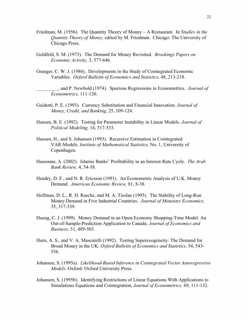
Figures 1 and 2 plots the calculated values of the recursive test statistics for the

M1 and profit-sharing deposits models, respectively. Note that these statistics are recursive likelihood-ratios normalized by the 5% critical value. Thus, calculated statistics that exceed unity imply rejection of the null hypothesis and suggest an unstable cointegrating relationship. The blue curve (BETA_Z) plots actual disequilibrium as a function of all short-run dynamics including seasonal dummy variables, while the black

16

curve (BETA_R) plots “clean” disequilibrium by correcting for short-run effects. We hold up the first fifteen years for the initial estimations. As we can see from both figures,

------------------------------------- Figures 1 and 2 about here

-------------------------------------------- the demands for the two aggregates appear stable over the long run when the models are corrected for short-run effects. Note that the long-run demand for money for the narrow aggregate (M1) is stable even without adjustments for short-run dynamics. This is because the initial hold-up period has similar characteristics as does the rest of the period. That is, M1 was interest free before and after the implementation of anti-usury law in Iran. In contrast, Figure (2) shows that without adjusting for short-run effects, the cointegrating parameters for the profit-sharing aggregate are unstable until about 1990, but then turns highly stable thereafter. A possible reason for this is that over almost 13 years of the initial period (up to 1979), the aggregate was bearing a predetermined interest rate. Consequently, a longer hold-up period is required for the initial estimation. As Figure (2) suggests, with an initial period of 1966-1990, the profit-sharing aggregate becomes stable over the long run irrespective of whether or not adjustments are made for short-run dynamics. 4. Concluding Remarks

We investigate the behavior of money demand in the Iranian economy using

quarterly data spanning the period 1966-2001. Since the mid-1980s, interest-based financial transactions have been banned in Iran. Consequently, this paper examines the demand for two alternative aggregates; namely, M1 and profit-sharing deposits. Unlike previous studies, our focus is on whether the estimated money demand models are policy invariant especially in the face of numerous exogenous shocks and changes in policy regimes that Iran has experienced in recent years. Besides being temporally stable (backward-looking behavior), we show that estimated money demand equations must also be policy invariant (forward-looking behavior) in order for these equations to be useful for monetary policy-making.

The conclusion which persistently emerges from a whole range of empirical

models and tests suggests that the estimated demand for M1 and profit-sharing deposits in Iran behave remarkably well and proved to be temporally stable both in the short and in the long run. Perhaps more importantly, these estimated money demand equations are also invariant to changes in policy regimes and other exogenous shocks that have characterized the recent monetary history of Iran. These findings prove robust and they stand up to various adjustments in model specifications. Although using different orientations and different methodologies, the results in this paper are broadly consistent with those reported recently by Darrat (2000, 2002) for Iran.

The results also show that, among the two alternative monetary aggregates, the

demand for profit-sharing deposits possesses the most stable and policy invariant function. Such a finding is consistent with prior theoretical evidence [for example, Khan

17

(1986), Chapra (1992)] which suggests that the profit-sharing banking scheme insulates the monetary system from interest-rate exposure risk and minimizes financial instability.

It is thus reasonable to argue that the elimination of interest-based financial

transactions in Iran and its replacement with the profit-sharing scheme in 1984 has not hampered the financial stability in the country. To the contrary, the introduction of profit-sharing has apparently strengthened Iran’s financial stability and provided the Central Bank with credible and reliable monetary policy instruments in their important and ongoing fight against inflationary pressures.

18

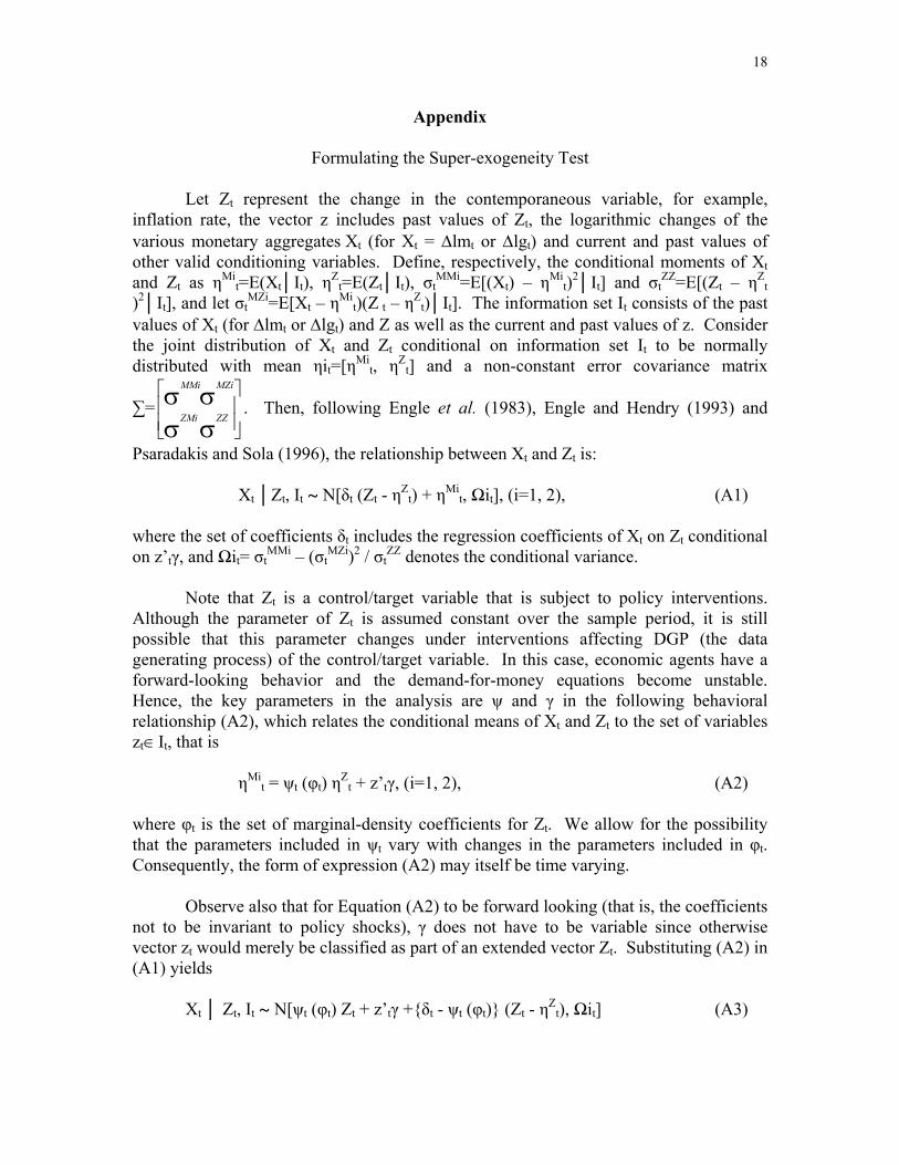
Appendix

Formulating the Super-exogeneity Test Let Zt represent the change in the contemporaneous variable, for example, inflation rate, the vector z includes past values of Zt, the logarithmic changes of the various monetary aggregates Xt (for Xt = ∆lmt or ∆lgt) and current and past values of other valid conditioning variables. Define, respectively, the conditional moments of Xt and Zt as ηMi

t=E(XtIt), ηZt=E(ZtIt), σt

MMi=E[(Xt) – ηMit)2It] and σt

ZZ=E[(Zt – ηZt

)2It], and let σtMZi=E[Xt – ηMi

t)(Z t – ηZt)It]. The information set It consists of the past

values of Xt (for ∆lmt or ∆lgt) and Z as well as the current and past values of z. Consider the joint distribution of Xt and Zt conditional on information set It to be normally distributed with mean ηit=[ηMi

t, ηZt] and a non-constant error covariance matrix

∑=

σσ

σσ

ZZ

MZi

ZMi

MMi

. Then, following Engle et al. (1983), Engle and Hendry (1993) and

Psaradakis and Sola (1996), the relationship between Xt and Zt is: Xt Zt, It ~ N[δt (Zt - ηZ

t) + ηMit, Ωit], (i=1, 2), (A1)

where the set of coefficients δt includes the regression coefficients of Xt on Zt conditional on z’tγ, and Ωit= σt

MMi – (σtMZi)2 / σt

ZZ denotes the conditional variance. Note that Zt is a control/target variable that is subject to policy interventions.

Although the parameter of Zt is assumed constant over the sample period, it is still possible that this parameter changes under interventions affecting DGP (the data generating process) of the control/target variable. In this case, economic agents have a forward-looking behavior and the demand-for-money equations become unstable. Hence, the key parameters in the analysis are ψ and γ in the following behavioral relationship (A2), which relates the conditional means of Xt and Zt to the set of variables zt∈It, that is

ηMi

t = ψt (φt) ηZt + z’tγ, (i=1, 2), (A2)

where φt is the set of marginal-density coefficients for Zt. We allow for the possibility that the parameters included in ψt vary with changes in the parameters included in φt. Consequently, the form of expression (A2) may itself be time varying. Observe also that for Equation (A2) to be forward looking (that is, the coefficients not to be invariant to policy shocks), γ does not have to be variable since otherwise vector zt would merely be classified as part of an extended vector Zt. Substituting (A2) in (A1) yields Xt Zt, It ~ N[ψt (φt) Zt + z’tγ +δt - ψt (φt) (Zt - ηZ

t), Ωit] (A3)

19

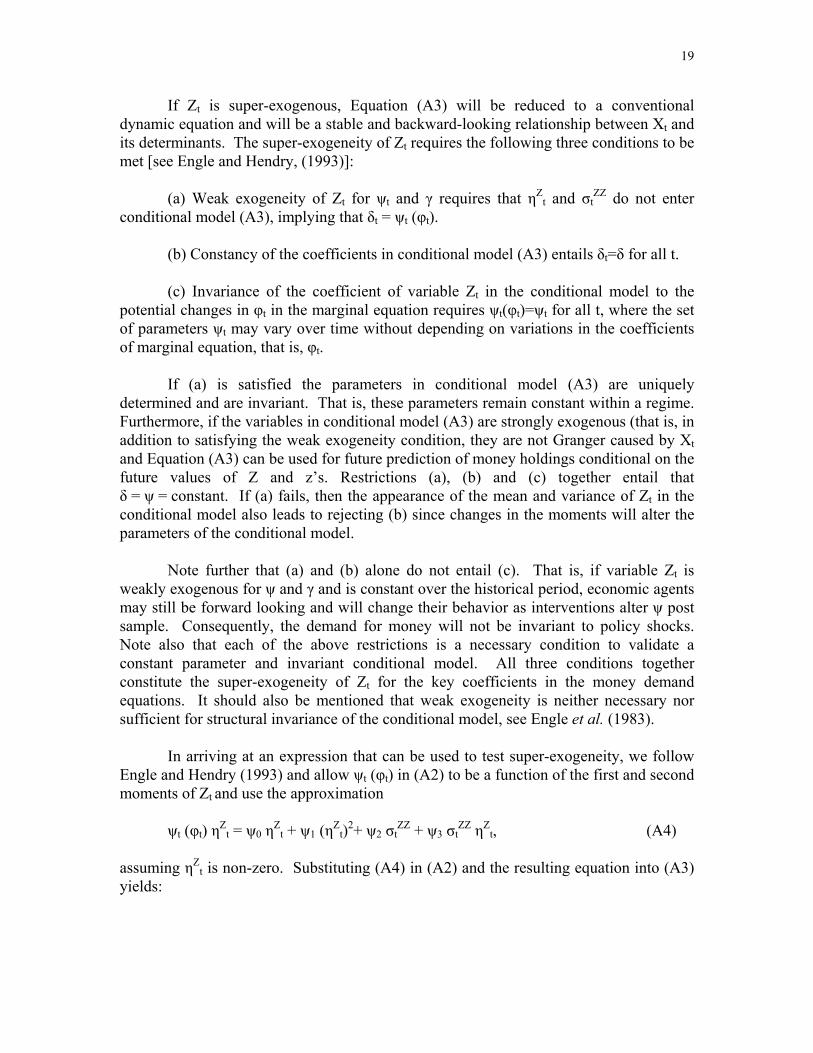
If Zt is super-exogenous, Equation (A3) will be reduced to a conventional dynamic equation and will be a stable and backward-looking relationship between Xt and its determinants. The super-exogeneity of Zt requires the following three conditions to be met [see Engle and Hendry, (1993)]:

(a) Weak exogeneity of Zt for ψt and γ requires that ηZ

t and σtZZ do not enter

conditional model (A3), implying that δt = ψt (φt). (b) Constancy of the coefficients in conditional model (A3) entails δt=δ for all t. (c) Invariance of the coefficient of variable Zt in the conditional model to the

potential changes in φt in the marginal equation requires ψt(φt)=ψt for all t, where the set of parameters ψt may vary over time without depending on variations in the coefficients of marginal equation, that is, φt. If (a) is satisfied the parameters in conditional model (A3) are uniquely determined and are invariant. That is, these parameters remain constant within a regime. Furthermore, if the variables in conditional model (A3) are strongly exogenous (that is, in addition to satisfying the weak exogeneity condition, they are not Granger caused by Xt and Equation (A3) can be used for future prediction of money holdings conditional on the future values of Z and z’s. Restrictions (a), (b) and (c) together entail that δ = ψ = constant. If (a) fails, then the appearance of the mean and variance of Zt in the conditional model also leads to rejecting (b) since changes in the moments will alter the parameters of the conditional model. Note further that (a) and (b) alone do not entail (c). That is, if variable Zt is weakly exogenous for ψ and γ and is constant over the historical period, economic agents may still be forward looking and will change their behavior as interventions alter ψ post sample. Consequently, the demand for money will not be invariant to policy shocks. Note also that each of the above restrictions is a necessary condition to validate a constant parameter and invariant conditional model. All three conditions together constitute the super-exogeneity of Zt for the key coefficients in the money demand equations. It should also be mentioned that weak exogeneity is neither necessary nor sufficient for structural invariance of the conditional model, see Engle et al. (1983). In arriving at an expression that can be used to test super-exogeneity, we follow Engle and Hendry (1993) and allow ψt (φt) in (A2) to be a function of the first and second moments of Zt and use the approximation ψt (φt) ηZ

t = ψ0 ηZt + ψ1 (ηZ

t)2+ ψ2 σtZZ + ψ3 σt

ZZ ηZt, (A4)

assuming ηZ

t is non-zero. Substituting (A4) in (A2) and the resulting equation into (A3) yields:

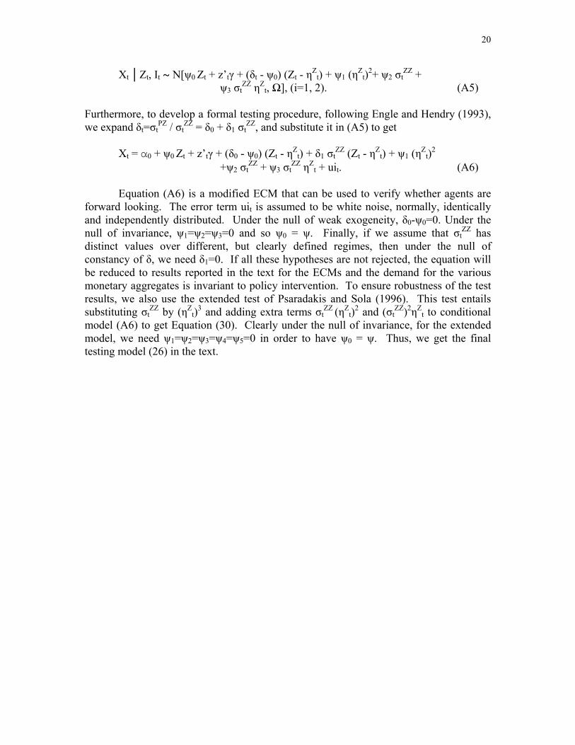
20

Xt Zt, It ~ N[ψ0 Zt + z’tγ + (δt - ψ0) (Zt - ηZt) + ψ1 (ηZ

t)2+ ψ2 σtZZ +

ψ3 σtZZ ηZ

t, Ω], (i=1, 2). (A5) Furthermore, to develop a formal testing procedure, following Engle and Hendry (1993), we expand δt=σt

PZ / σtZZ = δ0 + δ1 σt

ZZ, and substitute it in (A5) to get Xt = α0 + ψ0 Zt + z’tγ + (δ0 - ψ0) (Zt - ηZ

t) + δ1 σtZZ (Zt - ηZ

t) + ψ1 (ηZt)2

+ψ2 σtZZ + ψ3 σt

ZZ ηZt + uit. (A6)

Equation (A6) is a modified ECM that can be used to verify whether agents are forward looking. The error term uit is assumed to be white noise, normally, identically and independently distributed. Under the null of weak exogeneity, δ0-ψ0=0. Under the null of invariance, ψ1=ψ2=ψ3=0 and so ψ0 = ψ. Finally, if we assume that σt

ZZ has distinct values over different, but clearly defined regimes, then under the null of constancy of δ, we need δ1=0. If all these hypotheses are not rejected, the equation will be reduced to results reported in the text for the ECMs and the demand for the various monetary aggregates is invariant to policy intervention. To ensure robustness of the test results, we also use the extended test of Psaradakis and Sola (1996). This test entails substituting σt

ZZ by (ηZt)3 and adding extra terms σt

ZZ (ηZt)2 and (σt

ZZ)2ηZt to conditional

model (A6) to get Equation (30). Clearly under the null of invariance, for the extended model, we need ψ1=ψ2=ψ3=ψ4=ψ5=0 in order to have ψ0 = ψ. Thus, we get the final testing model (26) in the text.

21

References Aggarwal, R. K., and T. Yousef (2000). Islamic Banks and Investment Financing.

Journal of Money, Credit and Banking, 32, 93-120. Bashir, A. M. (2002). The Welfare Effects of Inflation and Financial Innovation in a

Model of Economic Growth -- An Islamic Perspective. Journal of Economic Studies, 29, 21-32.

Bashir, B. A. (1983). Portfolio Management of Islamic Banks. Journal of Banking and

Finance, 7, 339-354. Chapra, M. U. (1992). Islam and the Economic Challenge. Leichester, U. K.: The

Islamic Foundation. Cheung, Y., and K. S. Lai (1993). Finite-Sample Sizes of Johansen’s Likelihood Ratio

Tests for Cointegration. Oxford Bulletin of Economics and Statistics, 55, 313-328.

Darrat, A. F. (1988). The Islamic Interest-free Banking System: Some Empirical

Evidence. Applied Economics, 20, 417-425. __________ (2000). Monetary Stability and Interest-free Banking Revisited. Applied Economics Letters, 7, 803-806. __________ (2002). On the Efficiency of Interest-free Monetary System: A Case Study.

The Quarterly Review of Economics and Finance, 42, 747-764. Diz, A. C. (1970). Money and Prices in Argentina 1935-65. In Varieties of Monetary

Experiences, edited by D. I. Meiselman. Chicago: University of Chicago Press. Engle, R. F. (1982). Autoregressive Conditional Heteroskedasticity With Estimates of

the Variance of United Kingdom Inflation. Econometrica, 987-1007. _________, and D. F. Hendry (1993). Testing Superexogeneity and Invariance in

Regression Models. Journal of Econometrics, 56, 119-139. _________, and J. Richard (1983). Exogeneity. Econometrica, 51, 277-304. Engle, R. F., and C. W. J. Granger (1987). Co-integration and Error-Correction:

Representation, Estimation, and Testing. Econometrica, 55, 251-276. Favero, C., and D. F. Hendry (1992). Testing the Lucas Critique: A Review.

Econometric Reviews, 11, 265-306.

22

Friedman, M. (1956). The Quantity Theory of Money – A Restaurant. In Studies in the Quantity Theory of Money, edited by M. Friedman. Chicago: The University of Chicago Press.

Goldfeld, S. M. (1973). The Demand for Money Revisited. Brookings Papers on

Economic Activity, 3, 577-646. Granger, C. W. J. (1986). Developments in the Study of Cointegrated Economic

Variables. Oxford Bulletin of Economics and Statistics, 48, 213-218. _________, and P. Newbold (1974). Spurious Regressions in Econometrics. Journal of

Econometrics, 111-120. Guidotti, P. E. (1993). Currency Substitution and Financial Innovation. Journal of

Money, Credit, and Banking, 25, 109-124. Hansen, B. E. (1992). Testing for Parameter Instability in Linear Models. Journal of

Political Modeling, 14, 517-533. Hansen, H., and S. Johansen (1993). Recursive Estimation in Cointegrated

VAR-Models. Institute of Mathematical Statistics, No. 1, University of Copenhagen.

Hassoune, A. (2002). Islamic Banks’ Profitability in an Interest-Rate Cycle. The Arab

Bank Review, 4, 54-58. Hendry, D. F., and N. R. Ericsson (1991). An Econometric Analysis of U.K. Money

Demand. American Economic Review, 81, 8-38. Hoffman, D. L., R. H. Rasche, and M. A. Tieslan (1995). The Stability of Long-Run

Money Demand in Five Industrial Countries. Journal of Monetary Economics, 35, 317-339.

Hueng, C. J. (1999). Money Demand in an Open-Economy Shopping-Time Model: An

Out-of-Sample-Prediction Application to Canada. Journal of Economics and Business, 51, 489-503.

Hurn, A. S., and V. A. Muscatelli (1992). Testing Superexogeneity: The Demand for

Broad Money in the UK. Oxford Bulletin of Economics and Statistics, 54, 543-556.

Johansen, S. (1995a). Likelihood-Based Inference in Cointegrated Vector Autoregressive

Models. Oxford: Oxford University Press. Johansen, S. (1995b). Identifying Restrictions of Linear Equations With Applications to

Simulations Equations and Cointegration, Journal of Econometrics, 69, 111-132.

23

__________ and K. Juselius (1991). Testing Structural Hypotheses in a Multivariate

Cointegration Analysis of the PPP and the UIP for UK. Journal of Econometrics, 53, 211-244.

Khan, M. S. (1986). Islamic Interest-Free Banking: A Theoretical Analysis.

International Monetary Fund Staff Papers, 33, 1-27. __________, and A. Mirakhor (1990). Islamic Banking: Experience in the Islamic

Republic of Iran and Pakistan. Economic Development and Cultural Change, 38, 353-375.

Kia, A. (2003). Forward-Looking Agents and Macroeconomic Determinants of the

Equity Price in a Small Open Economy. Applied Financial Economics, 13, 37-54.

King, R., C. I. Plosser, J. H. Stock, and M. W. Watson (1991). Stochastic Trends and

Economic Fluctuations. American Economic Review, 81, 819-840. Lucas Jr., R. E. (1976). Econometric Policy Evaluation: A Critique. In Phillips Curve

and Labor Markets, edited by K. Brunner and A. H. Meltzer. Amsterdam: North-Holland.

__________ (1982). Interest Rates and Currency Prices in a Two-Country World.

Journal of Monetary Economics, 10, 335-359. Mankiw, N. G. (1991). The Reincarnation of Keynesian Economics. NBER Working

Papers No. 3885. Metin, K. (1998). The Relationship Between Inflation and the Budget Deficit in Turkey.

Journal of Business and Economic Statistics, 16, 412-422. Muscatelli, V. A., and F. Spinelli (2000). The Long-run Stability of the Demand for

Money: Italy 1861-1996. Journal of Monetary Economics, 45, 717-739. Nagayasu, J. (2003). A Re-examination of the Japanese Money Demand Function and

Structural Shifts. Journal of Policy Modeling, 25, 359-375. Osterwald-Lenum, M. (1992). A Note With Quantiles of the Asymptotic Distribution of

the Maximum Likelihood Cointegration Rank Test Statistics. Oxford Bulletin of Economics and Statistics, 54, 461-472.

Pagan, A. (1984). Econometric Issues in the Analysis of Regressions with Generated

Regressors. International Economic Review, 25, 221-247.

24

__________ (1986). Two Stage and Related Estimators and Their Applications. Review of Economic Studies, 53, 517-538.

Phillips, P. C. B. (1986). Understanding Spurious Regressions in Econometrics. Journal

of Econometrics, 37, 311-340. Psaradakis, Z., and M. Sola (1996). On the Power of Tests for Superexogeneity and

Structural Invariance. Journal of Econometrics, 72, 151-175. Sargent, T. J., and N. Wallace (1975). Rational Expectations, the Optimal Monetary

Policy Instruments, and Optimal Money Supply. Journal of Political Economy, 84, 241-254.

Stock, J. H., and M. W. Watson (1989). Interpreting the Evidence on Money-Income

Causality. Journal of Econometrics, 40, 161-182. ____________ (1993). A Simple Estimator of Cointegrating Vectors in Higher Order

Integrated Systems. Econometrica, 61, 783-820. Stockman, A. (1980). A Theory of Exchange Determination. Journal of Political

Economy, 88, 673-698. Tallman, E. W., D. Tang, and P. Wang (2003). Nominal and Real Disturbance and

Money Demand in Chinese Hyperinflation. Economic Inquiry, 41, 234-249. Yousefi, M., S. Abizadeh, and K. Maccormick (1997). Monetary Stability and

Interest-free Banking: the Case of Iran. Applied Economics, 29, 869-876.

Figure 1: Recursive Likelihood Ratio Tests for Interest-Free Monetary Aggregate

Test of known beta eq. to beta(t)

1 is the 5% significance level1984 1986 1988 1990 1992 1994 1996 1998 2000

0.00

0.25

0.50

0.75

1.00BETA_ZBETA_R

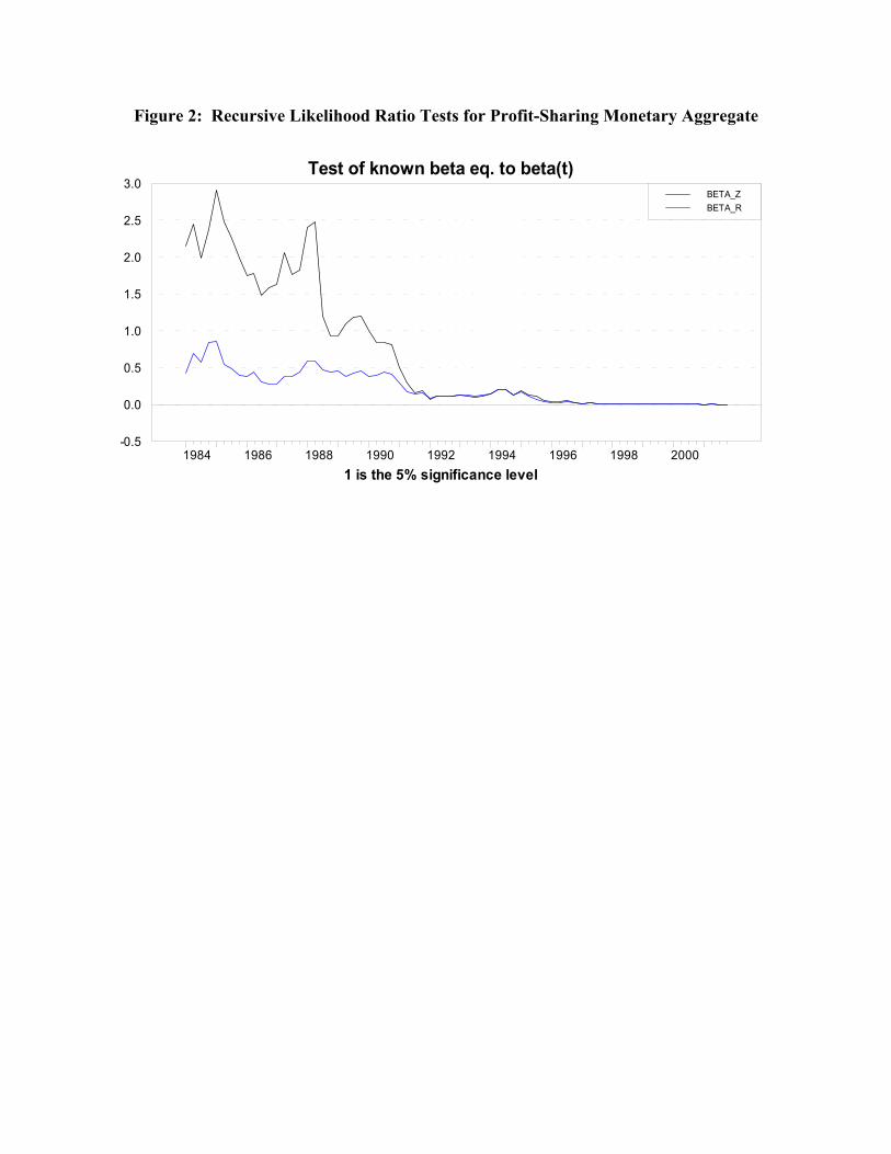
Figure 2: Recursive Likelihood Ratio Tests for Profit-Sharing Monetary Aggregate

Test of known beta eq. to beta(t)

1 is the 5% significance level1984 1986 1988 1990 1992 1994 1996 1998 2000

-0.5

0.0

0.5

1.0

1.5

2.0

2.5

3.0BETA_ZBETA_R

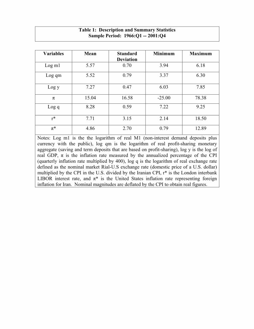
Table 1: Description and Summary Statistics Sample Period: 1966:Q1 -- 2001:Q4

Variables Mean Standard Deviation

Minimum Maximum

Log m1 5.57 0.70 3.94 6.18

Log qm 5.52 0.79 3.37 6.30

Log y 7.27 0.47 6.03 7.85

π 15.04 16.58 -25.00 78.38

Log q 8.28 0.59 7.22 9.25

r* 7.71 3.15 2.14 18.50

π* 4.86 2.70 0.79 12.89

Notes: Log m1 is the the logarithm of real M1 (non-interest demand deposits plus currency with the public), log qm is the logarithm of real profit-sharing monetary aggregate (saving and term deposits that are based on profit-sharing), log y is the log of real GDP, π is the inflation rate measured by the annualized percentage of the CPI (quarterly inflation rate multiplied by 400), log q is the logarithm of real exchange rate defined as the nominal market Rial-U.S exchange rate (domestic price of a U.S. dollar) multiplied by the CPI in the U.S. divided by the Iranian CPI, r* is the London interbank LIBOR interest rate, and π* is the United States inflation rate representing foreign inflation for Iran. Nominal magnitudes are deflated by the CPI to obtain real figures.

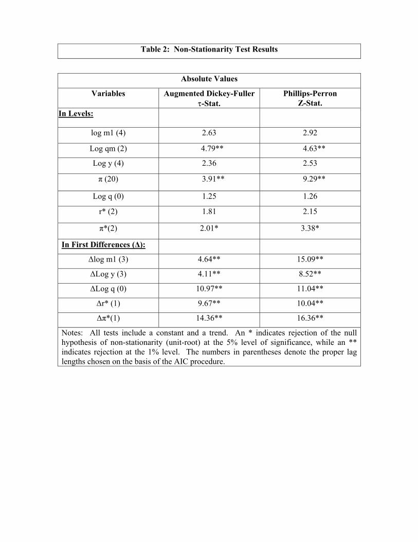
Table 2: Non-Stationarity Test Results

Absolute Values

Variables

Augmented Dickey-Fuller τ-Stat.

Phillips-Perron Z-Stat.

In Levels:

log m1 (4) 2.63 2.92

Log qm (2) 4.79** 4.63**

Log y (4) 2.36 2.53

π (20) 3.91** 9.29**

Log q (0) 1.25 1.26

r* (2) 1.81 2.15

π*(2) 2.01* 3.38*

In First Differences (∆):

∆log m1 (3) 4.64** 15.09**

∆Log y (3) 4.11** 8.52**

∆Log q (0) 10.97** 11.04**

∆r* (1) 9.67** 10.04**

∆π*(1) 14.36** 16.36**

Notes: All tests include a constant and a trend. An * indicates rejection of the null hypothesis of non-stationarity (unit-root) at the 5% level of significance, while an ** indicates rejection at the 1% level. The numbers in parentheses denote the proper lag lengths chosen on the basis of the AIC procedure.

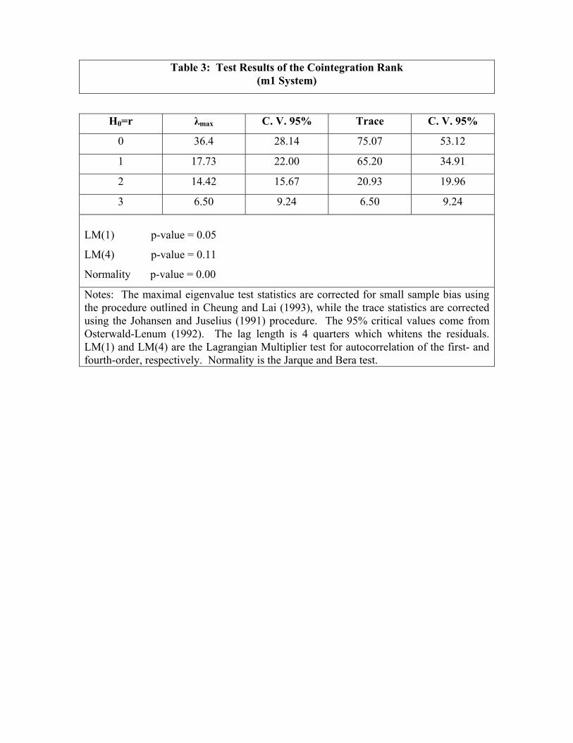
Table 3: Test Results of the Cointegration Rank (m1 System)

H0=r λmax C. V. 95% Trace C. V. 95%

0 36.4 28.14 75.07 53.12

1 17.73 22.00 65.20 34.91

2 14.42 15.67 20.93 19.96

3 6.50 9.24 6.50 9.24

LM(1) p-value = 0.05

LM(4) p-value = 0.11

Normality p-value = 0.00

Notes: The maximal eigenvalue test statistics are corrected for small sample bias using the procedure outlined in Cheung and Lai (1993), while the trace statistics are corrected using the Johansen and Juselius (1991) procedure. The 95% critical values come from Osterwald-Lenum (1992). The lag length is 4 quarters which whitens the residuals. LM(1) and LM(4) are the Lagrangian Multiplier test for autocorrelation of the first- and fourth-order, respectively. Normality is the Jarque and Bera test.

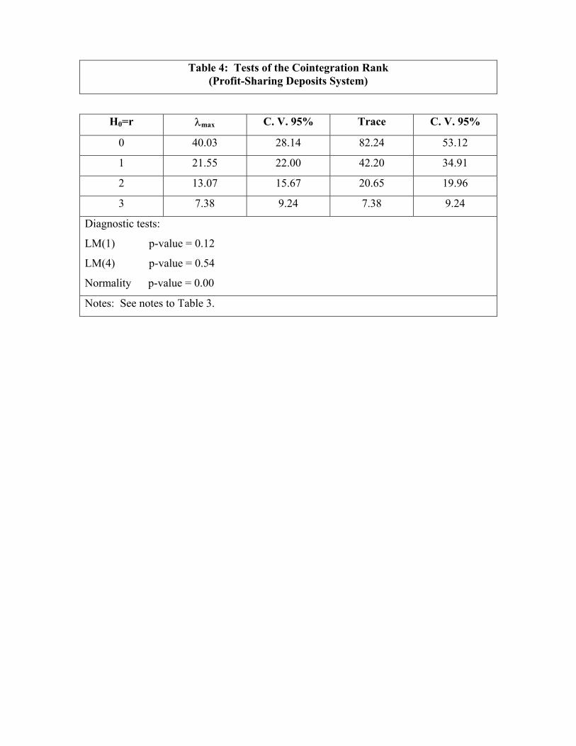
Table 4: Tests of the Cointegration Rank (Profit-Sharing Deposits System)

H0=r λmax C. V. 95% Trace C. V. 95%

0 40.03 28.14 82.24 53.12

1 21.55 22.00 42.20 34.91

2 13.07 15.67 20.65 19.96

3 7.38 9.24 7.38 9.24

Diagnostic tests:

LM(1) p-value = 0.12

LM(4) p-value = 0.54

Normality p-value = 0.00

Notes: See notes to Table 3.

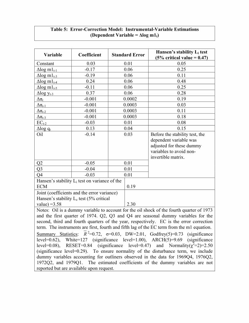
Table 5: Error-Correction Model: Instrumental-Variable Estimations (Dependent Variable = ∆log m1t)

Variable Coefficient Standard Error Hansen’s stability Li test (5% critical value = 0.47)

Constant 0.03 0.01 0.05 ∆log m1t-1 -0.17 0.06 0.25 ∆log m1t-3 -0.19 0.06 0.11 ∆log m1t-4 0.24 0.06 0.48 ∆log m1t-5 -0.11 0.06 0.25 ∆log yt-3 0.37 0.06 0.28 ∆πt -0.001 0.0002 0.19 ∆πt-1 -0.001 0.0003 0.03 ∆πt-2 -0.001 0.0003 0.11 ∆πt-3 -0.001 0.0003 0.18 ECt-2 -0.03 0.01 0.08 ∆log qt 0.13 0.04 0.15 Oil -0.14 0.03 Before the stability test, the

dependent variable was adjusted for these dummy variables to avoid non-invertible matrix.

Q2 -0.05 0.01 Q3 -0.04 0.01 Q4 -0.03 0.01 Hansen’s stability Li test on variance of the ECM

0.19

Joint (coefficients and the error variance) Hansen’s stability Lc test (5% critical value) =3.58

2.30

Notes: Oil is a dummy variable to account for the oil shock of the fourth quarter of 1973 and the first quarter of 1974. Q2, Q3 and Q4 are seasonal dummy variables for the second, third and fourth quarters of the year, respectively. EC is the error correction term. The instruments are first, fourth and fifth lag of the EC term from the m1 equation. Summary Statistics: R 2=0.72, σ=0.03, DW=2.01, Godfrey(5)=0.73 (significance level=0.62), White=127 (significance level=1.00), ARCH(5)=9.69 (significance level=0.08), RESET=0.84 (significance level=0.47) and Normality(χ2=2)=2.50 (significance level=0.29). To ensure normality of the disturbance term, we include dummy variables accounting for outliners observed in the data for 1969Q4, 1976Q2, 1972Q2, and 1979Q1. The estimated coefficients of the dummy variables are not reported but are available upon request.

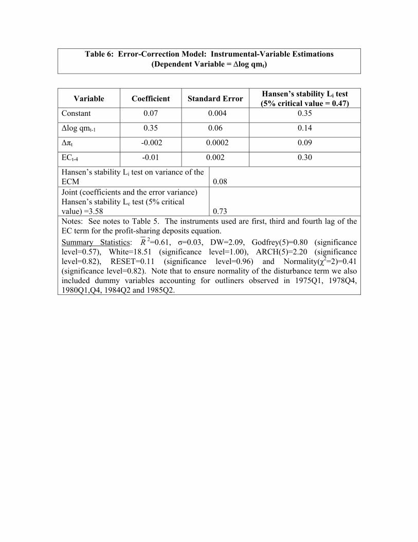
Table 6: Error-Correction Model: Instrumental-Variable Estimations (Dependent Variable = ∆log qmt)

Variable Coefficient Standard Error Hansen’s stability Li test (5% critical value = 0.47)

Constant 0.07 0.004 0.35

∆log qmt-1 0.35 0.06 0.14

∆πt -0.002 0.0002 0.09

ECt-4 -0.01 0.002 0.30

Hansen’s stability Li test on variance of the ECM

0.08

Joint (coefficients and the error variance) Hansen’s stability Lc test (5% critical value) =3.58

0.73

Notes: See notes to Table 5. The instruments used are first, third and fourth lag of the EC term for the profit-sharing deposits equation. Summary Statistics: R 2=0.61, σ=0.03, DW=2.09, Godfrey(5)=0.80 (significance level=0.57), White=18.51 (significance level=1.00), ARCH(5)=2.20 (significance level=0.82), RESET=0.11 (significance level=0.96) and Normality(χ2=2)=0.41 (significance level=0.82). Note that to ensure normality of the disturbance term we also included dummy variables accounting for outliners observed in 1975Q1, 1978Q4, 1980Q1,Q4, 1984Q2 and 1985Q2.

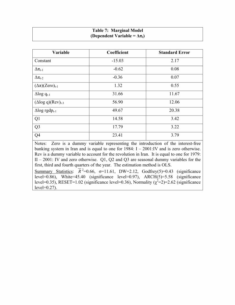
Table 7: Marginal Model (Dependent Variable = ∆πt)

Variable Coefficient Standard Error

Constant -15.03 2.17

∆πt-1 -0.62 0.08

∆πt-2 -0.36 0.07

(∆π)(Zero)t-1 1.32 0.55

∆log qt-1 31.66 11.67

(∆log q)(Rev)t-3 56.90 12.06

∆log rgdpt-1 49.67 20.38

Q1 14.58 3.42

Q3 17.79 3.22

Q4 23.41 3.79

Notes: Zero is a dummy variable representing the introduction of the interest-free banking system in Iran and is equal to one for 1984: I – 2001:IV and is zero otherwise. Rev is a dummy variable to account for the revolution in Iran. It is equal to one for 1979: II – 2001: IV and zero otherwise. Q1, Q2 and Q3 are seasonal dummy variables for the first, third and fourth quarters of the year. The estimation method is OLS. Summary Statistics: R 2=0.66, σ=11.61, DW=2.12, Godfrey(5)=0.43 (significance level=0.86), White=45.40 (significance level=0.97), ARCH(5)=5.58 (significance level=0.35), RESET=1.02 (significance level=0.36), Normality (χ2=2)=2.62 (significance level=0.27).

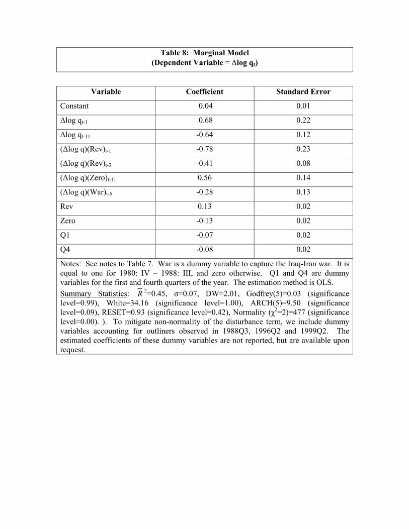
Table 8: Marginal Model (Dependent Variable = ∆log qt)

Variable Coefficient Standard Error

Constant 0.04 0.01

∆log qt-1 0.68 0.22

∆log qt-11 -0.64 0.12

(∆log q)(Rev)t-1 -0.78 0.23

(∆log q)(Rev)t-3 -0.41 0.08

(∆log q)(Zero)t-11 0.56 0.14

(∆log q)(War)t-6 -0.28 0.13

Rev 0.13 0.02

Zero -0.13 0.02

Q1 -0.07 0.02

Q4 -0.08 0.02

Notes: See notes to Table 7. War is a dummy variable to capture the Iraq-Iran war. It is equal to one for 1980: IV – 1988: III, and zero otherwise. Q1 and Q4 are dummy variables for the first and fourth quarters of the year. The estimation method is OLS. Summary Statistics: R 2=0.45, σ=0.07, DW=2.01, Godfrey(5)=0.03 (significance level=0.99), White=34.16 (significance level=1.00), ARCH(5)=9.50 (significance level=0.09), RESET=0.93 (significance level=0.42), Normality (χ2=2)=477 (significance level=0.00). ). To mitigate non-normality of the disturbance term, we include dummy variables accounting for outliners observed in 1988Q3, 1996Q2 and 1999Q2. The estimated coefficients of these dummy variables are not reported, but are available upon request.

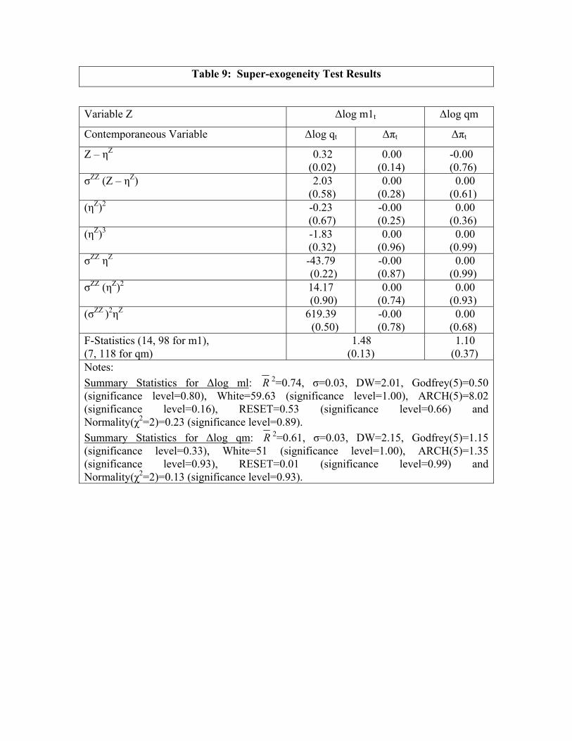
Table 9: Super-exogeneity Test Results

Variable Z ∆log m1t ∆log qm

Contemporaneous Variable ∆log qt ∆πt ∆πt

Z – ηZ 0.32 (0.02)

0.00 (0.14)

-0.00 (0.76)

σZZ (Z – ηZ) 2.03 (0.58)

0.00 (0.28)

0.00 (0.61)

(ηZ)2 -0.23 (0.67)

-0.00 (0.25)

0.00 (0.36)

(ηZ)3 -1.83 (0.32)

0.00 (0.96)

0.00 (0.99)

σZZ ηZ -43.79 (0.22)

-0.00 (0.87)

0.00 (0.99)

σZZ (ηZ)2 14.17 (0.90)

0.00 (0.74)

0.00 (0.93)

(σZZ )2ηZ 619.39 (0.50)

-0.00 (0.78)

0.00 (0.68)

F-Statistics (14, 98 for m1), (7, 118 for qm)

1.48 (0.13)

1.10 (0.37)

Notes: Summary Statistics for ∆log ml: R 2=0.74, σ=0.03, DW=2.01, Godfrey(5)=0.50 (significance level=0.80), White=59.63 (significance level=1.00), ARCH(5)=8.02 (significance level=0.16), RESET=0.53 (significance level=0.66) and Normality(χ2=2)=0.23 (significance level=0.89). Summary Statistics for ∆log qm: R 2=0.61, σ=0.03, DW=2.15, Godfrey(5)=1.15 (significance level=0.33), White=51 (significance level=1.00), ARCH(5)=1.35 (significance level=0.93), RESET=0.01 (significance level=0.99) and Normality(χ2=2)=0.13 (significance level=0.93).