modeling non performing loans probability in the ... · modeling non performing loans probability...

Dipartimento di Economia

No. 1 (May 10, 2009)

Modeling non performing loansprobability in the commercial banking

system: efficiency and effectivenessrelated to credit risk in Italy

Bernardo Maggi and Marco Guida

Editorial board

Margherita Carlucci; Claudio Sardoni; Luigi Solivetti; Giuseppe Venanzoni.

Modeling non performing loansprobability in the commercial banking

system: efficiency and effectivenessrelated to credit risk in Italy


Abstract

In this paper we model the effect of the non performing loans on the cost structure of the

commercial banking system. With this aim, we comment on an increase in the non performing

loans by studying the consequences of such a change on the cost function and compute the

probability of failure of maintaining a performing loan as such. In so doing we are convinced

that geography does matter and evaluate the risk propensity of the bank towards the non

performing loans accordingly. We finally stress that traditional efficiency indicators of cost

elasticity do not fit properly with such a problem and propose a measure based on the costs for

managing and monitoring the loans which, according to the related density function, will reveal

effectively as non performing.

JEL Classification: G21, D24, C33, C51, L23

Keywords: Non performing loans probability, Bank management, Cost function, Efficiency and

effectiveness indicators, Flexible forms

B. Maggi: Sapienza University of Rome, Faculty of Statistics ([email protected]); M. Guida:MediaCom, Business Insight Department ([email protected]). This research has been conducted with thejoint contribution of the authors although sections 1, 2, 4 and 6 are attributed to B. Maggi. while sections 3, 5 and 7to M. Guida.

Modelling non performing loans probability in the commercial banking system: efficiency and effectiveness related to credit risk in Italy

1

1 Introduction

So far the cost function in commercial banking studies has been widely used in literature under

various approaches. Notably we can briefly recall: the production approach, where inputs and

outputs are measured in physical quantities; the intermediation approach, that considers banks as

collecting and allocating funds in loans and other assets and where deposits are included among

the inputs; the asset approach that is similar to the intermediation approach but liabilities in

general are taken as inputs and assets as outputs; the value added approach, that takes any

balance sheet item as output if it absorbs a relevant share of capital and labor and the user cost

approach, which assumes that it is the net contribution to the bank revenue that defines inputs

and outputs (Resti (1997)). These approaches have been traditionally used in the literature to

study subjects like X-efficiency (Berger (1993), De Young (1997), Bauer (1990), Battese and

Coelli (1995)), scale and scope economies (Berger et al. (1997), Altunbas and Molyneux (1996),

Simper, (1999), Cavallo and Rossi (2001), Maggi and Rossi (2006), Vander Vennet (2002)),

technical progress (Dietsch and Lozano Vivas (2000), Bauer et al. (1993)) and the analytic

proprieties of flexible forms (McAllister and McManus (1993), Mitchell and Onvural (1996),

Berger et al. (1997), Berger and Mester (1997), Eastwood and Gallant (1991), Gallant (1981),

Caves et al. (1980), and Fuss and Waverman (1981)). However, little space has been given to the

loans that do not perform (NPL from now on) notwithstanding there are no doubts about the role

they play in affecting the cost function. Berger and De Young (1997) focused on problem loans

but without the quantification of their effects on the cost function, rather they analyzed how non

performing loans are linked to inefficiency. More recent researches started studying this problem

but with particular reference to both developing countries and emergent economies (Haunerand

and Peiris (2005), Matthewes et al. (2007)), for the implications -due to the insolvency of the

banking sector- on the economic growth and the performance of the banks respectively. As a

consequence, such studies just take a first, though important, step that consists either in netting

the loans of the non performing part or in considering NPL as an exogenous variable useful to

pick downward shifts in the profits. We go more into depth and propose a theoretical and

empirical analysis to place the problem of the non performing loans in the cost efficiency

framework. Our intention is to gauge how much of the efforts in managing and monitoring loans

succeed in preserving the bank from the non performing loans. In order to answer this question


2

we formalize a general methodology, independently of the contextual economic situation of the

country and capable to capture the linkage between NPL and cost structure of the commercial

banking system. We refer to the widest European bank and, specifically, to the Italian case where

problem loans did matter. We take into consideration the marginal effect of the non performing

loans on the operating costs by using and estimating a transformation function, that connects

loans with NPL. By exploiting this indirect relationship we also show a possible way out of the

dilemma of the simultaneous estimation between the cost function and NPL which, though logic

in principle, would alter the analysis with an overestimated efficiency for the additional variable

(NPL) in the cost function (Berger and De Young (1997)). We represent the link between loans

and non performing loans by stressing the role of the geographical position of the bank1. Such a

choice is also motivated by the importance that the economic specificities, associated to the

geographical localization of the loans, experimented especially by the US, played in the banking

sector recent international financial crises of 2007 and 2008. In so doing we evaluate and use the

density function of a loan to become non performing and another measure of probability that

connects loans with the more general concept of uncertain loans. We then study where, on

average, a bank is positioned with respect to the maximum sustainable level of NPL thus

evaluating the propensity of the bank to protect itself from the credit risk. Finally, we conclude

by proposing an index -that summarizes the issues stemming from the question we moved from-

of efficiency and effectiveness, related respectively to the management of the loans and to the

capacity to prevent non performing loans, according to the mentioned probability.

The paper is organized as follows. In the second section we present the basic theoretical

relationships to which we refer for the estimation. In the third section we reason on the variables

to include in the cost function in connection with the scope of our analysis and describe our data

set. In the fourth section we present the econometric analysis of such a function according to the

literature of the flexible functional forms. In the fifth section, where the focus is centered on the

problem of the NPL, we estimate their trade-off with loans and evaluate the attitude to the credit

risk of the bank. The sixth section reports the final calculation of the effect of NPL on the

marginal cost and some other efficiency and effectiveness indicators. The seventh section

concludes.

1 Actually the wide network of branches in Italy is suitable for analyzing this aspect.


3

2 Evaluating the effect of the non performing loans on the marginal cost:theoretical aspects

In this section we analyze the impact of a change in NPL on the bank cost structure. We face

such a problem by linking the bank’s marginal cost with non performing loans through the trade-

off between such a variable and the loans (L), that are the traditional output variable of the cost

function (C). To do so we employ the following transformation function:

(1) NPL = (L, ), L>0.

Such a function captures how a bank is more or less willing to accept problem loans in order to

increment its loan book, so that the more a bank will accept easily problem loans the more its

monitoring cost will be held down.

defines a vector of environmental variables ( i , i= 1,..., n) and the sign of the derivative

of NPL with respect to L is positive. We conceive the expression (1) is in line with the view that,

in our case study, the branches of a specific bank go under the same homogeneous monitoring

process and rules, that gives the possibility to represent the eventual inadequacy of such a

mechanism with a constant coefficient. However, as there may exist in specific regions particular

effects, associated to the local economy, which affect the transformation of the loans in non

performing ones, we will estimate an elasticity, between these two, per each area considered. The

Italian experience on this issue says clearly that, during recession periods, the South and the

Islands were the areas mostly expounded to the crisis, that is clearly attributable to the internal

degree of development reflected, after the downturn, either in the capacity of the existing firms

to adapt the production to the new profitable alternatives or in the birth of new ones in case of

bankruptcies. As an example, during the dramatic crisis of the first 90’s the percentage of NPL

upon L was about 10% on average in Italy but in the south almost the triple. Once the crisis re-

entered by means of the national money devaluation, the other areas -especially the North-

recovered promptly the previous condition contrarily to the South that was unable to exploit the

new favorable terms of trade. Still, other regional evidences support our conviction about this


4

strategy as pointed out by the well-known relevance that local factors assumed in the U.S.

financial crises of 2007 and 2008 relative to mortgage2.

Solving (1) for L and deriving C with respect to NPL, we get the marginal cost function:

(2)

NPLL

C

NPL

C

.1

,

which may be evaluated by adopting the following isoelastic form for the function:

(3))(

vLNPL , 0v1, n

iii 0 >0

where n represents the number of geographical partitions – later specified- of this study, is a

constant coefficient that picks the effect of the common inefficiencies in the monitoring process

related to the amount of loans and the elasticity ( ) is a function of the environmental dummy

variables on L and, for this reason, with the fundamental role of assessing the quality of the loans

according to the area considered. Taking derivatives we get:

(2’)

v

L

L

C

NPL

C

1

which is the final expression to be used for the calculation we are going to carry out in the sixth

section after having estimated the two components of (2). Such an expression represents a basic

result that consists in evaluating the change in the cost, in terms of loans management, associated

with an increase in the non performing loans according to (3). This effect is given by the

combination of the costs attributed to the loans management (L

C

) with the degree of accuracy

of the monitoring process, captured by the constant 1/ the specific regional effects, indicated by

1

, and an endogenous effect, associated to the level of loans 1

L . From (2’) it clearly

emerges that the more adequate is the monitoring process and the less penalizing are the regional

2 Indeed real estate is essentially a local investment notwithstanding the subprime mortgage crisis had globalimplications (on this point see IMF (2007)).


5

effects the higher the marginal cost to protect the quality of the loans. Then, we implement the

argumentations expounded above and model the relation between L and NPL for our case study

accordingly in order to focus on the following effect of NPL on C. Berger and De Young (1997)

concentrated on a different issue trying to shed some lights on the problem loans with an explicit

and detailed list of the possible inefficiencies by means of several Granger-causality

experiments. Though these attempts only state gross statistical associations with no economic

causations, they actually prove the relevance of the interrelationship between the cost function,

through inefficiency, and problem loans. However, such a settlement would imply to make a

simultaneous estimation between NPL and the cost function that in its turn would entail the

invalidation of the whole estimation for the overvaluation, in the NPL equation, of the efficiency.

In fact, this one would derive from a misleading –for pure statistical reasons- improvement of the

fit of the cost function, due to the additional variable NPL3. Then, our way of assigning the role

of interpreting the inefficiencies linked to NPL to the coefficients of the transformation function

(elasticizes, , and ), together with the separate estimation of the cost function adopted in

the fourth section, turns out to be coherent with the mentioned drawback. That is, as it will be

seen below in the rest of this paragraph, we circumvent such a problem by computing the

operating costs as an indirect function of NPL and making use of the probability of a loan to

become non performing in order to single out the part of the cost of managing loans attributed to

NPL. Moreover, as anticipated above, our treatment of problem loans is not exogenous for the

role attributed to L in the transformation function and consequently to 1

L in expression (2’).

In fact, as it will be specified in section 5, from the estimation of the elasticities, the higher the

level of loans the less the associated change in NPL, which means that, when the level of loans is

high, banks are less willing to risk in underwriting loans both with poor screening (skimping or

bad behavior according respectively to the prevalence of the negligence or the incapacity of the

management) and a priori risky (moral hazard behavior). In this way, the form of the

transformation function compounds, though synthetically, the problems posed in the literature at

the origin of NPL, whose endogeneity may be depicted with reference to L rather than –

3 Another inconvenient is the possibility to incur the multicollinearity between NPL and L.


6

simultaneously- on the cost function4. Differently, an exogenous form of inefficiency (bad luck)

is evaluated directly in the cost function by means of some fixed effects to correctly clean the

operating cost from the inefficiency not due to the management.

We then observe that, given the recommendations for the banks to control for the credit

risk5, they have to monitor the level of all uncertain loans (UL), that comprise NPL and other sort

of uncertain loans, according to: the value of the missing installments compared to the credit

granted, the country risk and the liability position of the borrower. Then, it may be reasonable to

presume an upper bound (UL ), that can be retained fixed at least for the short or medium run, in

line with the level of the stock of equity-i.e. the level of asset of the bank that can be used to face

the loss. On the basis of this reasoning one may replicate, in relative and more general terms, the

analysis till now developed to gauge the effect of a change in the NPL probability referred to

uncertain loans ( UL

NPLNPLp ULNPL _ ) on the operating cost relative to UL (c=C/UL ),

(2’’) ULNPLNPLp

c

NPL

C

_

,

that furnishes an evaluation of the expenses due to NPL per each single unit of allowed UL .

The usefulness of such a measure in marginal terms consists in its comparison with the yield

from L that may provoke either a revision of the loan book of the bank in favor of less risky

investors or a change in the loan conditions6, thus suggesting the opportunity, for next research,

of an extension of the present analysis to the different typology of loans.

However, if the interest of the researcher is in the evaluation of the probability concept of a

loan to become non performing ( L

NPLLp LNPL _ ), expression (3) is of help:

4 In a slightly different manner, as the inadequacies of the monitoring process of L may be described by thetransformation function with NPL -and the following definition of probability introduced below- we bypass the costfunction to represent the endogeneity of NPL.5 On this point the reader is referred to the Bank of Italy decree n. 229 dated 21/04/1999 and following updates.6 In 2007 and 2008 also Europe partly suffered from the US crisis. For instance in the U.K. there was a strongreduction of the loan- to-value ratio for mortgages.


7

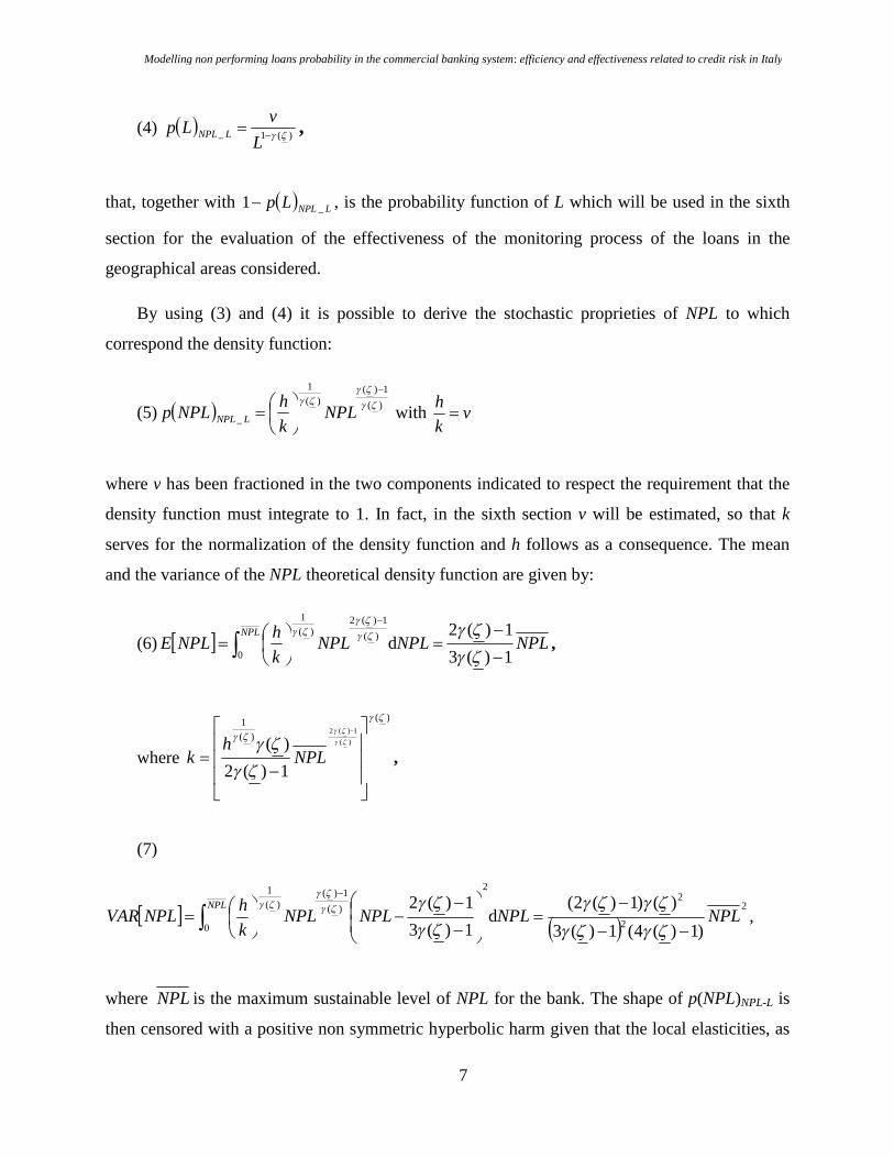
(4) )(1_

L

vLp LNPL ,

that, together with LNPLLp _1 , is the probability function of L which will be used in the sixth

section for the evaluation of the effectiveness of the monitoring process of the loans in the

geographical areas considered.

By using (3) and (4) it is possible to derive the stochastic proprieties of NPL to which

correspond the density function:

(5) )(

1)()(

1

_

NPL

k

hNPLp LNPL with v

k

h

where v has been fractioned in the two components indicated to respect the requirement that the

density function must integrate to 1. In fact, in the sixth section v will be estimated, so that k

serves for the normalization of the density function and h follows as a consequence. The mean

and the variance of the NPL theoretical density function are given by:

(6) NPLNPLNPLk

hNPLE

NPL

1)(3

1)(2d

0

)(

1)(2)(

1

,

where

)(

)(

1

)(

1)(2

1)(2

)(

NPLh

k ,

(7)

2

2

22

0

)(

1)()(

1

)1)(4(1)(3

)()1)(2(d

1)(3

1)(2NPLNPLNPLNPL

k

hNPLVAR

NPL

,

where NPL is the maximum sustainable level of NPL for the bank. The shape of p(NPL)NPL-L is

then censored with a positive non symmetric hyperbolic harm given that the local elasticities, as


8

will be seen in section 5, are all comprised between 0.5 and 17. NPL may be different according

to the areas considered, however, for simplicity’s sake, we can neglect this aspect without

limiting the analysis. Rather, we observe that, as the probability is truncated, it is possible to

compare the mean and the variance with the maximum non performing loans level, respectively

in absolute and squared value, to account for the different conditions of the areas under

examination in this regards and to evaluate the propensity of the bank to protect from the credit

risk. These results represent another advantage of having modeled the transformation function as

described above.

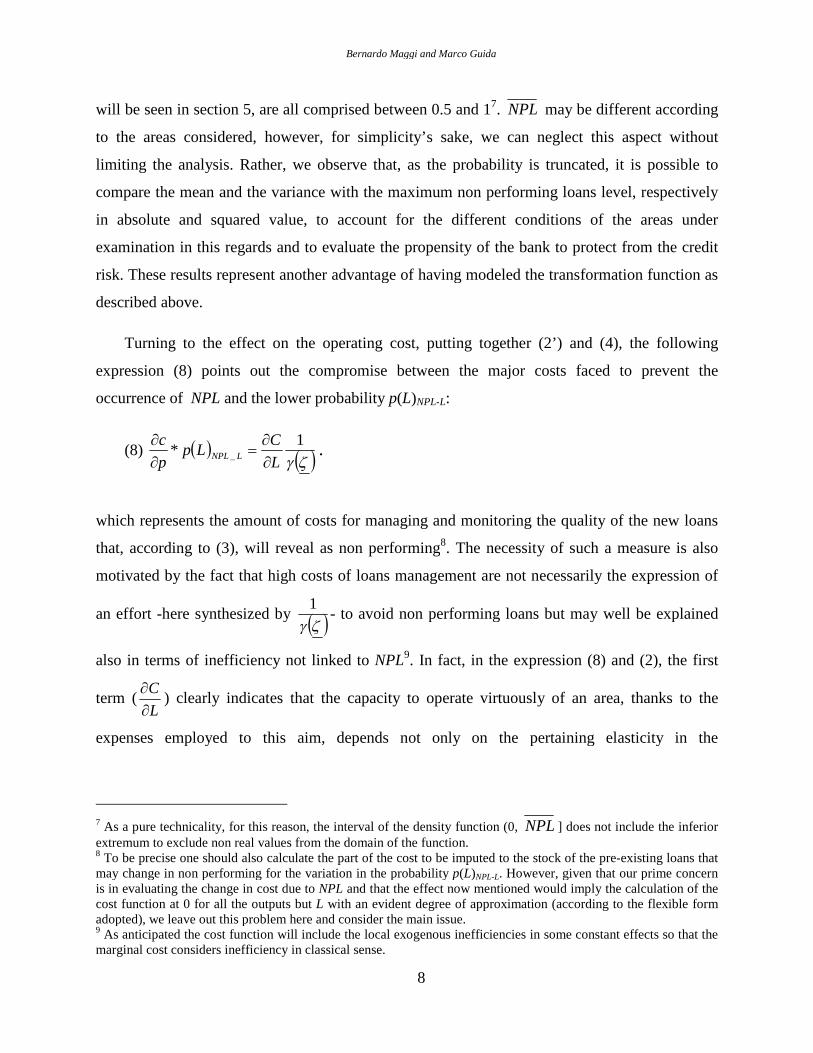
Turning to the effect on the operating cost, putting together (2’) and (4), the following

expression (8) points out the compromise between the major costs faced to prevent the

occurrence of NPL and the lower probability p(L)NPL-L:

(8) 1

* _L

CLp

p

cLNPL

.

which represents the amount of costs for managing and monitoring the quality of the new loans

that, according to (3), will reveal as non performing8. The necessity of such a measure is also

motivated by the fact that high costs of loans management are not necessarily the expression of

an effort -here synthesized by 1

- to avoid non performing loans but may well be explained

also in terms of inefficiency not linked to NPL9. In fact, in the expression (8) and (2), the first

term (L

C

) clearly indicates that the capacity to operate virtuously of an area, thanks to the

expenses employed to this aim, depends not only on the pertaining elasticity in the

7 As a pure technicality, for this reason, the interval of the density function (0, NPL ] does not include the inferiorextremum to exclude non real values from the domain of the function.8 To be precise one should also calculate the part of the cost to be imputed to the stock of the pre-existing loans thatmay change in non performing for the variation in the probability p(L)NPL-L. However, given that our prime concernis in evaluating the change in cost due to NPL and that the effect now mentioned would imply the calculation of thecost function at 0 for all the outputs but L with an evident degree of approximation (according to the flexible formadopted), we leave out this problem here and consider the main issue.9 As anticipated the cost function will include the local exogenous inefficiencies in some constant effects so that themarginal cost considers inefficiency in classical sense.


9

transformation function but also by the level of loans for scale economy considerations10. It goes

without saying that the two concepts may well not clash in the sense that an inefficient cost,

pointed out by a not optimal scale (highL

C

), may be effective as far as the monitoring of the

loans is concerned (low p(L)NPL-L).

3 Variables and Data

The specification we adopt for the cost function is that of the value added approach with three

outputs and two inputs. Among outputs we consider services, loans and deposits, among inputs

labor and capital. Deposits are regarded as an output, rather than an input, for the diminishing

importance of the interest rate on deposits still in the Italian commercial banking system.

The deposits variable comprises all funds raised from retail. The loans variable includes all

forms of performing and non-performing loans to customers. The services variable is constructed

as the total value of services income11. All variables are expressed in nominal (euro) values at

constant prices (year 2000).

The cost associated with these inputs is composed of total personnel expenses and non-staff

expenses i.e. operative costs12. The labor price is calculated as total personnel cost divided by the

number of employees. As regards the capital price a common way to calculate it would be that of

dividing the cost of capital (operative cost associated with capital expenses) by fixed assets net

of depreciation. However, given the lack in our data set of the stock of fixed capital of each

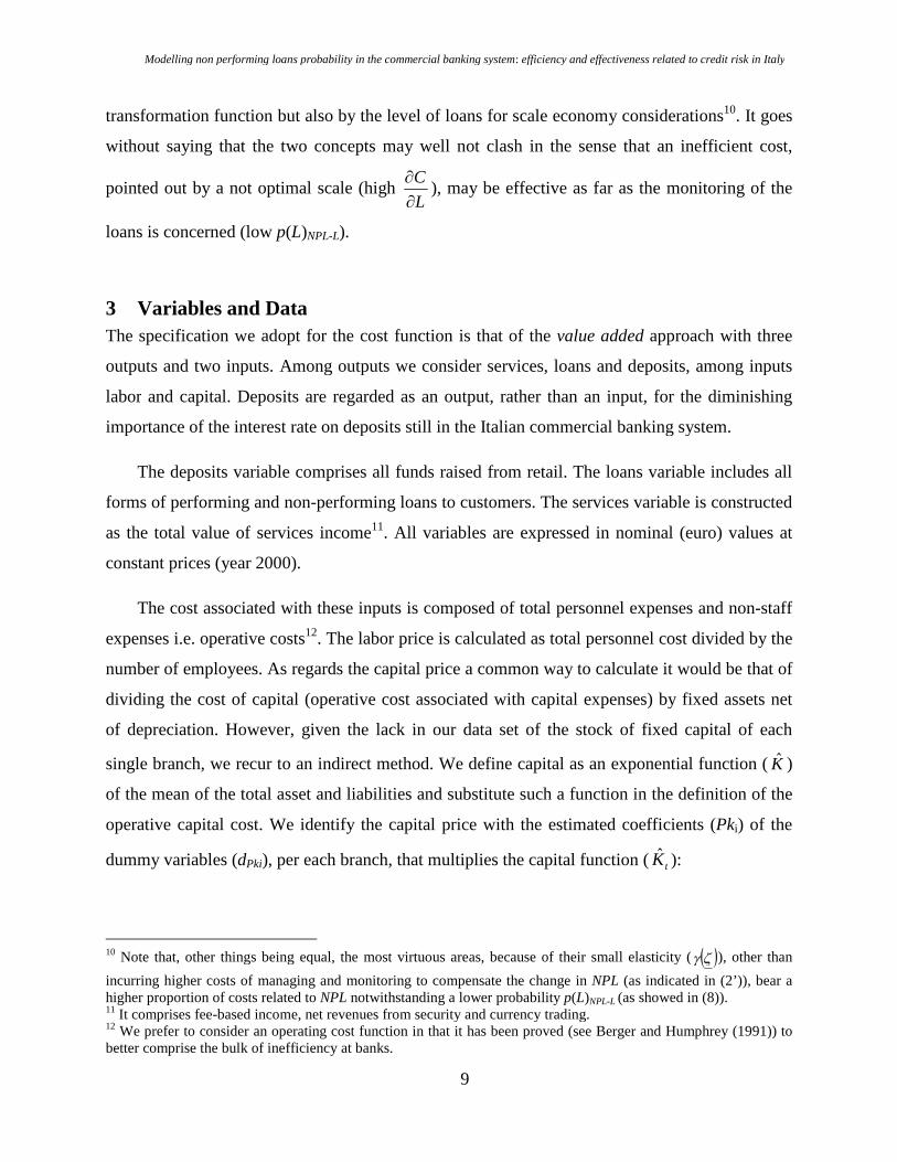
single branch, we recur to an indirect method. We define capital as an exponential function ( K̂ )

of the mean of the total asset and liabilities and substitute such a function in the definition of the

operative capital cost. We identify the capital price with the estimated coefficients (Pki) of the

dummy variables (dPki), per each branch, that multiplies the capital function ( tK̂ ):

10 Note that, other things being equal, the most virtuous areas, because of their small elasticity ( ), other than

incurring higher costs of managing and monitoring to compensate the change in NPL (as indicated in (2’)), bear ahigher proportion of costs related to NPL notwithstanding a lower probability p(L)NPL-L (as showed in (8)).11 It comprises fee-based income, net revenues from security and currency trading.12 We prefer to consider an operating cost function in that it has been proved (see Berger and Humphrey (1991)) tobetter comprise the bulk of inefficiency at banks.


10

(9) Capital costit = ti

d

i KPk Pki ˆ968

1

, tK̂ = ttt LAmean , , i = 1,.......,968; t= 2003, 2004

where it is the random error and is a constant parameter obtained, together with Pki, by using

the LSDV estimator for specific branches fixed effects13. We use N=968 branches after having

dropped all the branches with missing and non-reliable values.

The database consists of a panel across two years (T=2) 2003-2004 provided by The Office

of Planning and Control of Banca di Roma-Capitalia now included in the Unicredit Group. Our

interest in such a bank is due both to its relevance in Europe, where it counts the widest network

of branches among all European banks, and to the problems associated with uncertain loans it

incurred in 2000-2001 (Senate of Italian Republic, Act n.2-00110, 22/01/2002) that gave rise to

the following operation of securitization through the constitution and the management of

apposite special purpose vehicles. The period considered in this study -though short for

availability of the NPL variable- gives the opportunity to pick the consequences of such facts in

the data. These aspects are proved to be relevant as confirmed by the crisis of the European

credit market of 2008 to which Unicredit took an active part.

As regards uncertain loans, they have different definition across European countries. More

specifically, considering NPL, we find in Italy the most critical condition that a loan is

considered non performing in case of the borrower’s insolvency stated by a court while in other

countries it suffices a delay in the payment. Further, the possibility to have tax concessions, for

corrections of uncertain loans by means of coverage funds, is also different across European

countries being in Italy very discouraging with 0.6% of the amount accounted for (Ministry of

Finance decree –CIR- n. 207 /E dated 16/11/2000, art. 23). Such considerations are reflected in

the following fig. 1 where the scenario for the some major European countries is described as far

as uncertain loans are concerned.

13 Results available upon request.


11

fig. 1: Uncertain loans in Europe

Average data 2003-2004.

On the vertical axis is represented the level of funds accumulated for the coverage of the

uncertain loans14 while the horizontal axe and the dimension of the rings represent respectively

the percentage of UL upon L and of UL upon equity (E). As anticipated in the previous section,

the stock of equity represents the level of asset to face the general risk of the considered banking

system other than that of NPL, and comprises capital shares, reserves, profits and capital gains.

As can be easily checked, Italy is in a critical position with respect to these variables. Even if its

low level of coverage is certainly also due to the above mentioned discouraging fiscal rules, this

does not justifies the high proportions of UL/L and UL/E. Consequently, from an empirical point

of view, we deem relevant to examine the Italian case by focusing on UL and, among them, in

particular on NPL.

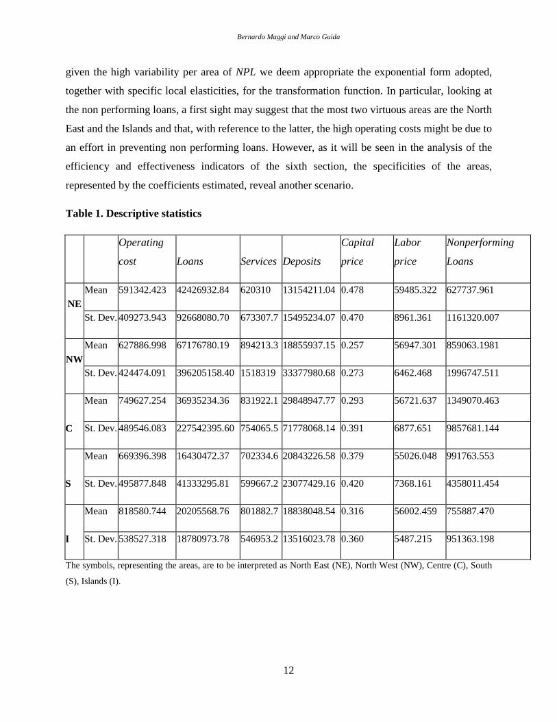
In table 1 are reported some descriptive statistics of the variables used to carry out the

estimation of the following sections. We consider the mean and the standard deviation for the

areas used in the estimations. We first observe the opportunity of an econometric analysis, given

the high level of variance compared to the mean. Second, we underline the relevance of the

partition adopted in light of the differences among the means of the areas considered. Third,

14 Note that it is also possible to observe a level of coverage funds that, prudentially, exceeds that of the uncertainloans as in Spain and Portugal.


12

given the high variability per area of NPL we deem appropriate the exponential form adopted,

together with specific local elasticities, for the transformation function. In particular, looking at

the non performing loans, a first sight may suggest that the most two virtuous areas are the North

East and the Islands and that, with reference to the latter, the high operating costs might be due to

an effort in preventing non performing loans. However, as it will be seen in the analysis of the

efficiency and effectiveness indicators of the sixth section, the specificities of the areas,

represented by the coefficients estimated, reveal another scenario.

Table 1. Descriptive statistics

Operating

cost Loans Services Deposits

Capital

price

Labor

price

Nonperforming

Loans

NE

Mean 591342.423 42426932.84 620310 13154211.04 0.478 59485.322 627737.961

St. Dev. 409273.943 92668080.70 673307.7 15495234.07 0.470 8961.361 1161320.007

NW

Mean 627886.998 67176780.19 894213.3 18855937.15 0.257 56947.301 859063.1981

St. Dev. 424474.091 396205158.40 1518319 33377980.68 0.273 6462.468 1996747.511

C

Mean 749627.254 36935234.36 831922.1 29848947.77 0.293 56721.637 1349070.463

St. Dev. 489546.083 227542395.60 754065.5 71778068.14 0.391 6877.651 9857681.144

S

Mean 669396.398 16430472.37 702334.6 20843226.58 0.379 55026.048 991763.553

St. Dev. 495877.848 41333295.81 599667.2 23077429.16 0.420 7368.161 4358011.454

I

Mean 818580.744 20205568.76 801882.7 18838048.54 0.316 56002.459 755887.470

St. Dev. 538527.318 18780973.78 546953.2 13516023.78 0.360 5487.215 951363.198

The symbols, representing the areas, are to be interpreted as North East (NE), North West (NW), Centre (C), South

(S), Islands (I).


13

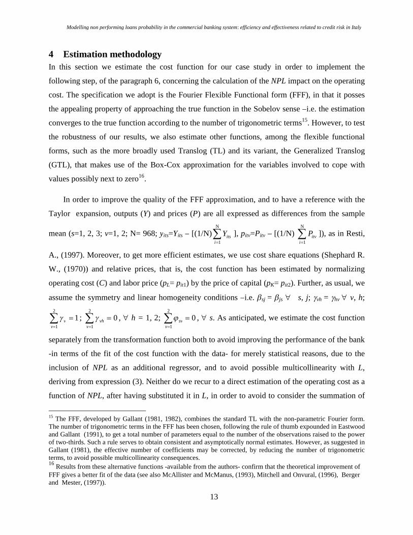
4 Estimation methodology

In this section we estimate the cost function for our case study in order to implement the

following step, of the paragraph 6, concerning the calculation of the NPL impact on the operating

cost. The specification we adopt is the Fourier Flexible Functional form (FFF), in that it posses

the appealing property of approaching the true function in the Sobelov sense –i.e. the estimation

converges to the true function according to the number of trigonometric terms15. However, to test

the robustness of our results, we also estimate other functions, among the flexible functional

forms, such as the more broadly used Translog (TL) and its variant, the Generalized Translog

(GTL), that makes use of the Box-Cox approximation for the variables involved to cope with

values possibly next to zero16.

In order to improve the quality of the FFF approximation, and to have a reference with the

Taylor expansion, outputs (Y) and prices (P) are all expressed as differences from the sample

mean (s=1, 2, 3; v=1, 2; N= 968; yits=Yits – [(1/N)

N

1iitsY ], pitv=Pitv – [(1/N)

N

1iitvP ]), as in Resti,

A., (1997). Moreover, to get more efficient estimates, we use cost share equations (Shephard R.

W., (1970)) and relative prices, that is, the cost function has been estimated by normalizing

operating cost (C) and labor price (pL= pit1) by the price of capital (pK= pit2). Further, as usual, we

assume the symmetry and linear homogeneity conditions –i.e. sj = js s, j; vh = hv v, h;

12

1

v

v ; 02

1

v

vh , h = 1, 2; 02

1

v

sv , s. As anticipated, we estimate the cost function

separately from the transformation function both to avoid improving the performance of the bank

-in terms of the fit of the cost function with the data- for merely statistical reasons, due to the

inclusion of NPL as an additional regressor, and to avoid possible multicollinearity with L,

deriving from expression (3). Neither do we recur to a direct estimation of the operating cost as a

function of NPL, after having substituted it in L, in order to avoid to consider the summation of

15 The FFF, developed by Gallant (1981, 1982), combines the standard TL with the non-parametric Fourier form.The number of trigonometric terms in the FFF has been chosen, following the rule of thumb expounded in Eastwoodand Gallant (1991), to get a total number of parameters equal to the number of the observations raised to the powerof two-thirds. Such a rule serves to obtain consistent and asymptotically normal estimates. However, as suggested inGallant (1981), the effective number of coefficients may be corrected, by reducing the number of trigonometricterms, to avoid possible multicollinearity consequences.16

Results from these alternative functions -available from the authors- confirm that the theoretical improvement ofFFF gives a better fit of the data (see also McAllister and McManus, (1993), Mitchell and Onvural, (1996), Bergerand Mester, (1997)).


14

the errors of the two equations and skip the problem of the generated regressors (Pagan (1986)).

However, to cope with any regional exogenous effect, connected to inefficiency, we include in

the cost function specific dummies for areas as well as for time to account for changes in

technology. Time (year 2003) and geographical areas (North East (NE), North West (NW),

Centre (C), South (S), Islands (I)) dummy variables are respectively represented by dyear and

g , g = 1, 2, 3, 417. and are random errors. SUR estimation is straightforward.

FFF and the cost share are (for simplicity of notation we omit deponents i and t):

(10)

jj

ssjss

ss

K

yyyp

Clnln2/1lnln

3

1

3

1

3

10

K

L

sssv

K

L

K

L

p

py

p

p

p

plnlnln)2/1(ln

3

1

2111 + g

ggdyear

4

1

+

4

1

4

1

4

1

4

1

4

1

4

1

cossincossinu l

luulu l

luulu

uuu

uu xxxxxx

4

1

4

1

44

1

4

1

4

cossinu

mlul lm

ulmu

mlul lm

ulm xxxxxx u, l, m = 1, 2, 3, 4

(11)

k

L

ssi

kL

Lp

py

pp

CS lnln

)/ln(

ln11

3

11

For coherency purposes we have transformed the original dependent variables in radiants to

be used in the trigonometric part of the function. The transformation is that of Berger, A.,

Leusner, J. and Mingo, J. (1997). According to this transformation xu is the equivalent of ys for s

= 1, 2, 3 while for u=4 it refers to pL/pK. Due to multicollinearity we consider the Fourier

approximation till the third term and drop some of the regressors18.

17 As usual, the coefficients of these variables are to be evaluated as the difference from the ones not listed in theestimation results that are year 2004 and NE, both represented by 0.18 All estimations and calculations were made with the econometric software Stata 9.


15

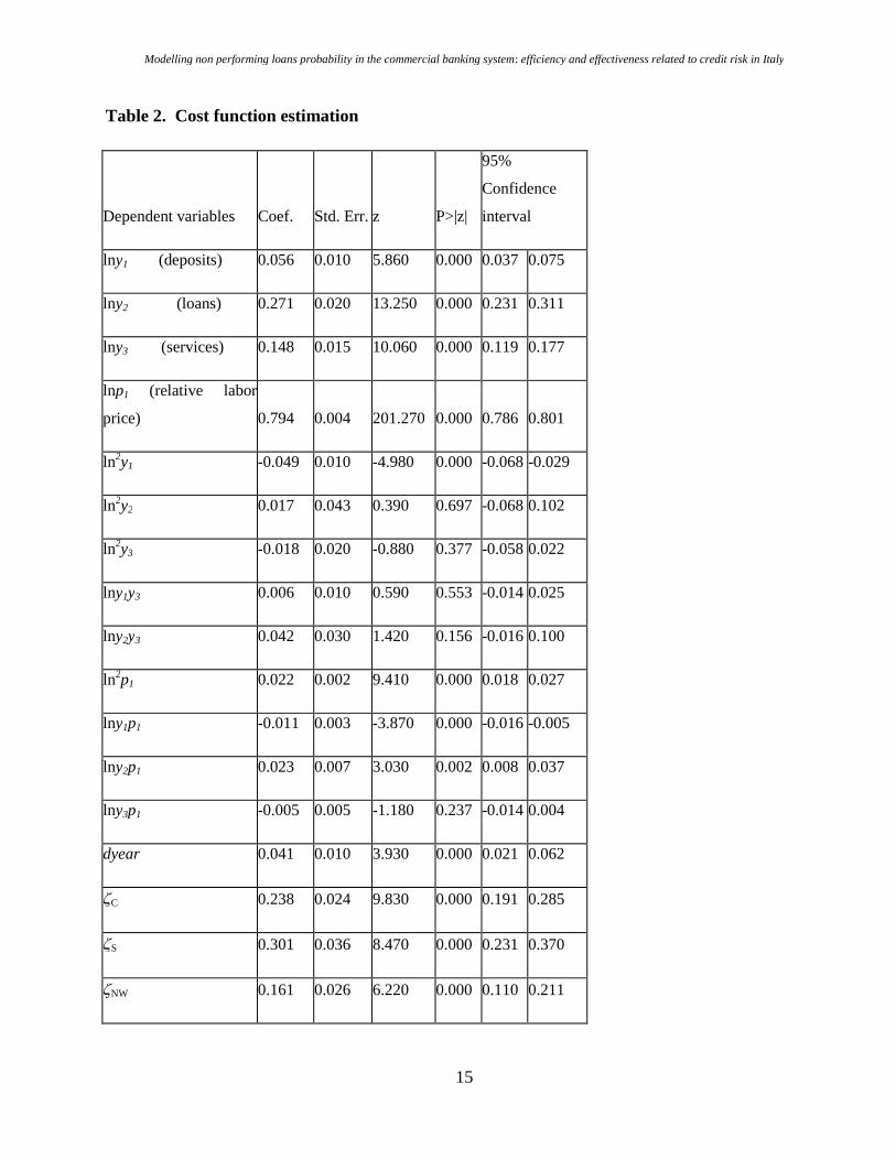
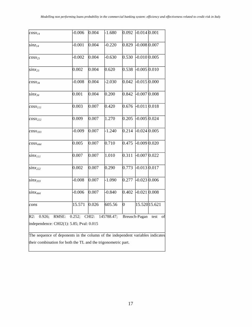
Table 2. Cost function estimation

Dependent variables Coef. Std. Err. z P>|z|

95%

Confidence

interval

lny1 (deposits) 0.056 0.010 5.860 0.000 0.037 0.075

lny2 (loans) 0.271 0.020 13.250 0.000 0.231 0.311

lny3 (services) 0.148 0.015 10.060 0.000 0.119 0.177

lnp1 (relative labor

price) 0.794 0.004 201.270 0.000 0.786 0.801

ln2y1 -0.049 0.010 -4.980 0.000 -0.068 -0.029

ln2y2 0.017 0.043 0.390 0.697 -0.068 0.102

ln2y3 -0.018 0.020 -0.880 0.377 -0.058 0.022

lny1y3 0.006 0.010 0.590 0.553 -0.014 0.025

lny2y3 0.042 0.030 1.420 0.156 -0.016 0.100

ln2p1 0.022 0.002 9.410 0.000 0.018 0.027

lny1p1 -0.011 0.003 -3.870 0.000 -0.016 -0.005

lny2p1 0.023 0.007 3.030 0.002 0.008 0.037

lny3p1 -0.005 0.005 -1.180 0.237 -0.014 0.004

dyear 0.041 0.010 3.930 0.000 0.021 0.062

C 0.238 0.024 9.830 0.000 0.191 0.285

S 0.301 0.036 8.470 0.000 0.231 0.370

NW 0.161 0.026 6.220 0.000 0.110 0.211


16

I 0.202 0.026 7.690 0.000 0.151 0.254

cosx1 0.005 0.008 0.650 0.519 -0.010 0.020

sinz1 -0.015 0.007 -2.020 0.043 -0.030 -0.001

cosx2 -0.017 0.007 -2.340 0.019 -0.032 -0.003

sinz2 0.001 0.007 0.100 0.918 -0.014 0.015

cosx3 -0.012 0.007 -1.660 0.098 -0.027 0.002

sinx3 -0.013 0.008 -1.730 0.084 -0.028 0.002

cosx4 -0.019 0.008 -2.410 0.016 -0.034 -0.004

sinx4 -0.022 0.008 -2.930 0.003 -0.037 -0.007

cosx11 -0.011 0.007 -1.570 0.117 -0.026 0.003

sinx11 -0.006 0.007 -0.740 0.457 -0.020 0.009

cosx22 0.020 0.007 2.790 0.005 0.006 0.035

sinx22 -0.004 0.007 -0.580 0.560 -0.019 0.010

cosx33 0.011 0.007 1.460 0.145 -0.004 0.025

sinx33 -0.009 0.007 -1.170 0.242 -0.023 0.006

cosx44 0.008 0.008 1.010 0.314 -0.007 0.023

sinx44 -0.017 0.007 -2.260 0.024 -0.031 -0.002

cosx12 0.002 0.004 0.680 0.496 -0.005 0.010

sinx12 -0.003 0.004 -0.850 0.398 -0.011 0.004

cosx13 0.001 0.004 0.280 0.781 -0.006 0.008

sinx13 0.003 0.004 0.920 0.357 -0.004 0.011


17

cosx14 -0.006 0.004 -1.680 0.092 -0.014 0.001

sinz14 -0.001 0.004 -0.220 0.829 -0.008 0.007

cosx23 -0.002 0.004 -0.630 0.530 -0.010 0.005

sinx23 0.002 0.004 0.620 0.538 -0.005 0.010

cosx34 -0.008 0.004 -2.030 0.042 -0.015 0.000

sinx34 0.001 0.004 0.200 0.842 -0.007 0.008

cosx111 0.003 0.007 0.420 0.676 -0.011 0.018

cosx222 0.009 0.007 1.270 0.205 -0.005 0.024

cosx333 -0.009 0.007 -1.240 0.214 -0.024 0.005

cosx444 0.005 0.007 0.710 0.475 -0.009 0.020

sinx111 0.007 0.007 1.010 0.311 -0.007 0.022

sinx222 0.002 0.007 0.290 0.773 -0.013 0.017

sinx333 -0.008 0.007 -1.090 0.277 -0.023 0.006

sinx444 -0.006 0.007 -0.840 0.402 -0.021 0.008

cons 15.571 0.026 605.56 0 15.52015.621

R2: 0.926; RMSE: 0.252; CHI2: 145788.47; Breusch-Pagan test of

independence: CHI2(1): 5.85; Pval: 0.015

The sequence of deponents in the column of the independent variables indicates

their combination for both the TL and the trigonometric part.


18

We get reasonable values for the parameters estimation19. In particular, looking at the

elasticities of the first order terms, we find, among outputs, a significant, though small,

importance attributed to deposits (0.056), other than, as it may be more easily expected, to loans

(0.271) and services (0.148). This result is justified by the large network of branches that

deposits still imply nowadays, notwithstanding the ongoing tendency to reduce their role in favor

of services. The sharp reduction of the bank’s main profit source from interest income, is forcing

banks to find new proceeds alternatives to deal with. In this respect, services are taking on an

increasingly growing importance, thus explaining their consistent impact on the cost function. As

far as loans are concerned, we observe the largest effect on operating costs.

As regards the management of inputs, due to the small flexibility of the Italian labor market,

the labor factor has a greater impact (0.794) on the cost function than capital (0.216).

From the side of the time and geographical variables, the former reveals a significant decreasing

costs over time for the improvement in the management due to the increasing technical

progress20, the latter highlights a strong and significant penalizing effect of the environment

mostly concentrated in the areas of Centre and South, followed by Islands. On the contrary,

North East and North West are the most efficient areas.

5 Estimating the transformation function “” an evaluation of the creditrisk

To estimate the transformation function, commented in section 2, we employ the vector of

environmental variables ( ) used in section 4 and the LSDV estimator for fixed effects on slope

19 Results from TL and GTL -obtained with the use of the cost shares as well- confirmed that from FFF. Inparticular, the use of the Box-Cox approximation in the GTL specification avoids any possible doubt, on the stabilityof the coefficients, in case of small values, of the variables expressed in logs.20 Bauer et al. 1993 provide evidence from the US banking system on the validity of the use of the change in thetime dummy variables as an indicator of the effect of the technical progress. Actually, in 2004, “Banca di Roma”was awarded with the Guido Carli prize as the best retail bank for the innovations due to information and technologyinvestments.


19

here related to the different geographical areas21. The following table 3 shows the results of the

estimation of the expression (3), reported below for our case study:

(3’) LLLLLvNPL lnlnlnlnlnlnln IISSCCNWNWNE

Table 3. function estimation

Coef. Std. Err. z P>|z|

NE 0.8153 0.02736 29.8 0.00 0.815

NW 0.01161 0.00897 1.29 0.196 0.827

C 0.03177 0.00814 3.9 0.00 0.847

S 0.03601 0.00891 4.04 0.00 0.851

I 0.02677 0.01235 2.17 0.03 0.842

ln(v) -1.3123 0.43891 -2.99 0.003

Number of observations = 1936;

F( 5, 1930) = 204.40;

Prob > F = 0.0000;

R-squared = 0.3462;

Adj R-squared = 0.3445;

Root MSE = 1.3705.

where is the residual term and NW, C, S, I, are calculated, for the areas indicated, as

differentials, from the elasticity NE. The elasticities, referred to the former areas, are then

obtained by summing such differentials to NE and reported in the last column.

21 We choose this method instead of the alternative of GLS for the complete and exhaustive longitudinal series ofour data set that suggests us to propend for fixed rather than random effects. However, also in case of correctness ofthe random effects we would have obtained consistent estimates, given that LSDV consistency rely on N*T which,in our case, is sufficiently large. Differently, in case of wrong hypothesis about random effect, consistency wouldhave been undermined by GLS for omitted variables.


20

Results confirm our expectation on the relevance of the geographical partition considered.

Specifically, Islands and South perform worse than Centre, North West and North East

differently from what evidenced at a first stage by the descriptive statistics of table 1. The latter

two are not significantly different and exhibit the smallest sensibility of NPL to L. Moreover, as

one can easily check, by inserting the estimated elasticities in formulae (6) and (7), the average

NPL of the more performing areas (NW, NE) shows a percentage of the maximum sustainable

NPL of rather 40%. In a different way, in the case of the South, such a percentage approaches the

central value of the density function in that the exponential form of the transformation function

tends to assume a linear form as the elasticity of the considered area tends to one. On the other

side, as regards the variance, the percentage of the examined areas are similar, standing around

the 0.9% of the maximum squared value. These results, obtained from the estimation of the

theoretical density function of the NPL, signal the relevance of the geographical localization of

the bank and reveal that, though under the same common rules, the branches may exhibit

important differences that might be capable, once the losses from NPL are capitalized, to

compromise the performance of the bank. Further, a remarkable and warning fact is that, also in

the mentioned performing areas, the estimated mean is not so far from the central value of the

probability density function thus revealing the tendency of the bank to move away from a policy

oriented to protect itself from the risk. This result follows directly from the form of the

transformation function that is below the straight line, NPL = v L, but as much close to it

according to the local elasticity. The straight line, therefore, may be considered as a term of

reference to evaluate the degree of riskiness of the bank given that if it lies upon it the proportion

of NPL on L remains neutrally the same. Our elasticities are all around 0.8, revealing, coherently

with the considerations on the average NPL, an attitude to the risk slightly below the neutrality,

that appears in contradiction with the credit protection as characteristic of commercial banks.

Then, as anticipated in section 2, we have two considerations concerning the risk. First, we have

to look at how far from the origin the position of the bank loans in the selected area is located.

Second, we have to check the level of the corresponding elasticity that shows the specific

propensity of the areas to risk. Moreover, we observe that the use of the transformation function,

to compare different regions as to the risk linked to NPL, may be fruitfully exploited to develop

an analysis centered on a comparison among different banks. However, as said before, to


21

implement the next step, of evaluating the NPL effect on the operating cost, we need to associate

such a result with the estimated cost function.

6 Calculating the effect of nonperforming loans on the marginal cost:efficiency and effectiveness indicators

In this section we first stress the inadequacy of the traditional indicators in dealing with the

problem of nonperforming loans, then implement the calculation expounded in formula (2’) and

present some indicators in order to underline properly the differences in the cost structure across

the areas considered.

As regards the traditional efficiency indicators, we put in evidence their weakness by

observing that they do not characterize properly the geographical partitions taken into account.

As an example let’s consider the elasticity of cost to loans and, in this specific case, to non

performing loans. Such a fact may be an implication of the application of the vigilance

instructions, on behalf of the monetary authority, that may drive branches to reach, according to

this indicators, an homogenous result. Turning to the analysis developed in the previous sections,

the characterization of the geographical partition emerges. In fact, as indicated in table 4, from

the effect of a change in the non performing loans on the cost function –or alternatively of the

NPL probability, ULNPLNPLp _ , on c- it is possible to observe that C performs better than NE

while NO is in the best position and S and I in the worst one. We gauge such differences as

extremely relevant to be pointed out for the possibility to control costs by increasing or reducing

the level of loans and non performing loans according to the performance of the different areas.

Table 4. Efficiency and effectiveness indicators

geographical areas NE NO C S I

Elasticity-C,L 0.0560 0.0560 0.0560 0.0560 0.0560

Elasticity-C,NPL 0.0678 0.0687 0.0661 0.0658 0.0665

ULNPLNPLp

c

NPL

C

_

0.091 0.053 0.072 0.118 0.143


22

(C/L)* 0.781 0.524 1.138 2.287 2.270

p(L)NPL-L 0.011 0.012 0.019 0.023 0.019

p(L)NPL-L * c/p 0.001 0.000636 0.00136 0.00271 0.00271

*values expressed in thousands. Calculations are in the sample means of the areas.

Actually, such a description reflects that the less scoring areas suffer from an overburden of

costs in managing with NPL. However, this result is to be deepened to understand if, in the areas

where the managing costs of NPL are high (as from C/NPL of formula (2’)), such expense

indicates an effort appositely done to avoid non performing loans or an inefficiency in loans

management. From the calculation of the density function p(L)NPL-L presented in formula (4) -that

is by emphasizing the role of the effectiveness- we can unfold such a doubt by evidencing that

the expenses of NE to monitoring loans are effective with the lowest probability to generate

NPL, whilst the position of the Centre is to be reconsidered with an high p(L)NPL-L due an

ineffective marginal cost in managing with loans. In other words, the most virtuous areas are

capable to compensate a change in NPL with a consistent amount of good loans though facing

higher cost of monitoring and management. Moreover, from the derivative of C with respect to

L, the supremacy of the North is confirmed especially against the South and the Islands where

the change in the operating costs due to loans is more than triple thus revealing an evident

inefficiency in loans management.

To conclude, the results from (2’) might drive to wrong conclusions if not read together with

(4). In fact, looking at the measure proposed in formula (8), the consequent ranking in table 4

states as less efficient the areas where the marginal cost of loans are not coupled with a low

probability p(L)NPL-L. We deem such indicator as reliable in that combines both the aspects of the

expenses –for credit management- and their efficacy -referred to the proportion of the costs of

managing and monitoring the loans that will become non performing.


23

7 Conclusions and further remarks

In this study we move from the consideration of the lack, in the literature of efficiency in the

banking sector, of an accurate dealing with the NPL. We formalize a model for the placement of

the NPL in the cost function thus trying to fill somehow the hiatus in this respect and giving

further potential to the tools so far available. We answer the question of how much of the efforts

in terms of costs for managing and monitoring loans succeed in preserving the bank from the non

performing loans i. e. we measure the change in the cost function due to new incoming L and

select, proportionally, the expenses associated with the generated NPL. Our framework is based

on the consideration that NPL is not directly an item of the cost function but can be viewed as a

transformation of the loans that stands for the bank’s trade-off between these two. From this

representation we derive the density function of a loan to become non performing which gives

the possibility to study how, on average, the bank is positioned with respect to the maximum

sustainable level of NPL and to evaluate the propensity of the bank to protect himself from the

credit risk. This is done by assigning a particular role to the geographical aspects that are found

to be relevant both in the transformation and cost function estimation. This allows for the

possibility to make considerations on the efficiency and effectiveness of the costs management

referred to both loans and non performing loans and, consequently, to control costs with

reference to the regions considered. We find that traditional output-elasticity indicators do not fit

properly with the problem of NPL and propose more representative measures.

We find that the effect of a change in the probability of an uncertain loan to become non

performing is extremely costly for the banking system thus further encouraging the research in

this field with an analysis that, from the one hand, disentangles the specific categories of loans

and their degree of risk and, from the other hand, could test the effectiveness of such credit

policies.

Acknowledgments

We are grateful to the University of Rome “La Sapienza” for the funds provided to support this

research (Progetto di ricerca Università 2007, C26A07ZJJ2). We thank the Office of Planning

and Control of Banca di Roma and the Investor Relations office of Capitalia-Unicredit for the

support given and for the extremely helpful suggestions and comments. In particular we are


24

indebted to Lawrence Kay, Paola De Rita, Francesco Masera, Paolo Giacomin and Antonio

Sansonetti. The usual disclaimer always applies.

References

Altunbas, Y., Molyneux, P., (1996), “Economies of scale and scope in European banking”,

Applied Financial Economics, n. 6 (4), pp. 367-75.

Battese, G. E., Coelli, T., (1995), “A Model for technical inefficiency effects in a stochastic

frontier production function for panel data”, Empirical Economics, n. 20, pp. 325-332.

Bauer, P., (1990), “Recent developments in the econometric estimation of frontiers”, Journal of

Econometrics, n. 46, pp. 39-56.

Bauer, P., Berger, A.N., Humphrey, D.B., (1993), “Efficiency and productivity growth in US

banking”, in: Fried, H.O., Lovell, C.A.K., Schmidt, S.S. ( Eds.), “The measurement of

productive efficiency: techniques and applications”, Oxford University Press, pp. 386-413.

Berger, A, N., (1993), “Distribution free estimates of efficiency in the U.S. banking industry and

tests of the standard distributional assumptions”, The Journal of Productivity Analysis, n. 4, pp.

261-292.

Berger, A, N., Humphrey D., B, 1991, “The dominance of inefficiencies over Scale and Product

Mix Economies in Banking”, Journal of Monetary Economics 28, 117- 148.

Berger, A. N., De Young, R., (1997), “Problem loans and cost efficiency in commercial banks”,

Journal of Banking and Finance, n. 21, pp. 849-870.

Berger A., Leusner J., Mingo J., (1997), “The efficiency of bank branches”, Journal of Monetary

Economics, n° 1, n. 40, pp. 141-162.

Berger, A. N., Mester, L. J., (1997), “Inside the black box: what explains differences in the

efficiency of financial institutions”, Journal of Banking and Finance, n. 21, pp. 895-947.

Cavallo, L., Rossi, S. P. S., (2001), “Scale and scope economies in the European banking

systems”, Journal of Multinational Financial Management, n. 11, pp. 515-531.


25

Caves, D. W., Christensen, L. R., Tretheway, M. W., (1980), “Flexible cost function for

multiproduct firms”, Review of Economics and Statistics, n. 62, pp. 185-202.

De Young, R., (1997), “A Diagnostic test for the distribution-free efficiency estimator: An

example using U.S. commercial bank data”. European Journal of Operational Research, n. 98,

pp. 243-249.

Dietsch, M., Lozano Vivas, A., (2000), “How the environment determines the efficiency of

banks: a comparison between the French and Spanish banking industries”, Journal of Banking

and Finance, n. 26, pp. 985-1004.

Eastwood, B. J., Gallant, A.R., (1991), “Adaptive Rules for semi-nonparametric estimators that

achieve asymptotic normality”, Econometric Theory, n. 7, pp. 307-340.

Gallant, R., (1981), “On the bias of flexible functional forms and an essentially unbiased form”,

Journal of Econometrics, n. 15, pp. 211-245.

Gallant, R., (1982), “Unbiased determination of production technologies”, Journal of

Econometrics, n. 20, pp. 285-323.

Hauner, D., Peiris, S. J., (2005), “Bank efficiencies and competition in low income countries: the

case of Uganda”, IMF working paper, wp/05/240, International Monetary Fund.

IMF, (2007), Global Financial Stability Report, April.

Maggi, B., Rossi, S., (2006), “An efficiency analysis of banking systems: a comparison of

European and United States large commercial banks using different functional form”, The Icfai

Journal of Bank Management, ICFAI University Press, n° 2, pp. 7-35.

Matthewes, K., Guo, J. Zhang, N., (2007), “Rational inefficiency and non-performing loans in

Chinese Banking: a non parametric bootstrapping approach”, Cardiff economic working papers,

E2007/5, Cardiff University, U.K.

McAllister, P.H., McManus, D., (1993), “Resolving the scale efficiency puzzle in banking”,

Journal of Banking and Finance, n. 17, pp. 389-405.


26

Mitchell, K., Onvural, N. M., (1996), “Economies of scale and scope at large commercial banks:

Evidence from the Fourier flexible functional form”, Journal of Money, Credit and Banking, n.

28, pp. 178-199.

Pagan, A., (1986), “Two stage and related estimators and their applications”, Review of

Economic Studies, n. 54, pp. 517-538.

Resti, A., (1997), “Evaluating the cost efficiency of the Italian banking system: what can be

learnt from the joint application of parametric and non-parametric techniques”, Journal of

Banking and Finance, n. 21, pp. 221-250.

Shephard, R. W., (1970), “Theory of cost and production function”, Princeton University Press,

Princeton, NJ.

Simper, R., (1999), “Economies of scale in the Italian saving banking industry”, Applied

Financial Economics, n. 9, pp. 11-19.

Vander Vennet, R., (2002), “Cost and profit efficiency of financial conglomerates and universal

banks in Europe”, Journal of Money, Credit and Banking, n. 34, pp. 254-282.

modeling non performing loans probability in the ... · modeling non performing loans probability...

Documents