MODELING OF A DISTILLATION COLUMN

USING BOND GRAPHS

by

Braden Alan Brooks

A Thesis Submitted to the Faculty of the

Department of Electrical & Computer Engineering

In Partial Fulfillment of the Requirements For the Degree of

MASTER OF SCIENCE WITH A MAJOR IN ELECTRICAL ENGINEERING

in the Graduate College

THE UNIVERSITY OF ARIZONA

Copyright © Braden Alan Brooks 1993

1 9 9 3

1

STATEMENT BY AUTHOR

This thesis has been submitted in partial fulfillment of requirements for an advanced degree at the University of Arizona and is deposited in the University Library to be made available to borrowers under rules of the Library.

Brief quotations from this thesis are allowable without special permission, provided that accurate acknowledgment of source is made. Requests for permission for extended quotation from or reproduction of this manuscript in whole or in part may be granted by the copyright holder. SIGNED:

APPROVAL BY THESIS DIRECTOR

This thesis has been approved on the date shown below: François E. Cellier Date Associate Professor of Electrical and Computer Engineering

2

ACKNOWLEDGMENT

To let understanding stop at what cannot be understood is a high attainment. Those who cannot do this will be destroyed on the lathe of heaven.

Tchuang-tse

The author would like to thank the universe for not being as perversely

ordered as once thought.

Also, considerable thanks goes to the patience and faith of my advisor,

Dr. François Cellier, and to my parents, Billy and Jean Brooks.

3

TABLE OF CONTENTS

LIST OF FIGURES.......................................................................................................6

LIST OF TABLES.........................................................................................................9

ABSTRACT ..................................................................................................................10

1.0 INTRODUCTION ................................................................................................11 1.1 The basics of a distillation column ........................................................11 1.2 The basics of bond graphs ......................................................................16 1.3 The assumptions of a distillation column ............................................19

2.0 THE ELEMENTS OF A DISTILLATION COLUMN ......................................22 2.1 Mass balance.............................................................................................22 2.2 Energy balance .........................................................................................25 2.3 Hydraulic (pressure and volume flow) ................................................28 2.4 Vapor-liquid equilibrium (chemical potential and molar flow) .......42 2.5 Heat (temperature and entropy)............................................................50 2.6 Equation of state.......................................................................................52 2.7 Condenser and receiver ..........................................................................56 2.8 Reboiler......................................................................................................62 2.9 Control system..........................................................................................68

3.0 MODELING WITH BOND GRAPHS ...............................................................70 3.1 Bond graph representation of the model..............................................70

3.1.1 Hydraulic ....................................................................................72 3.1.2 Thermal........................................................................................78 3.1.3 Chemical......................................................................................82 3.1.4 Combining hydraulic, thermal, and chemical .......................84

3.2 Hierarchical bond graph representation ..............................................88

4.0 THE DISTILLATION COLUMN AS A SYSTEM ............................................94 4.1 The early models ......................................................................................94 4.2 The Gallun model ....................................................................................96 4.3 Modifying the Gallun model..................................................................102 4.4 Simulation results ....................................................................................106

5.0 CONCLUSION.....................................................................................................115 5.1 Future work in distillation.......................................................................115

4

5.2 Future work in bond graphs ...................................................................117

TABLE OF CONTENTS — Continued

APPENDIX A: NOTATION .....................................................................................121

APPENDIX B: GALLUN’S DISTILLATION COLUMN .......................................128 B.1 The equations of the model.....................................................................128 B.2 DYMOLA code of Gallun’s model.........................................................136 B.3 DYMOLA assessment of Gallun’s model .............................................159

APPENDIX C: ACSL CODE FOR SIMPLE DISTILLATION COLUMN MODEL..............................................................................................167

APPENDIX D: ACSL CODE FOR COMPLEX DISTILLATION COLUMN MODEL..............................................................................................188

REFERENCES..............................................................................................................213

5

LIST OF FIGURES

1.1. The basic stage of a distillation column...........................................................12

1.2. The basic distillation column.............................................................................13

2.1. Bond graph of liquid mass balance equation (2-8).........................................25

2.2. Internal energy elements....................................................................................28

2.3. Bond graph of fluid flow, equation (2-28) .......................................................33

2.4. The hydraulic variables in a distillation column stage..................................34

2.5. Bond graph of downcomer hydraulics, equation (2-31) ...............................36

2.6. Bond graphs of Francis weir formula, .............................................................40

2.7. Transformer representing chemical to hydraulic power conversion..........45

2.8. The bond graph of the condenser, equations (2-70).......................................58

2.9. Cooling water flow in condenser......................................................................59

2.10. Bond graph of pump ........................................................................................60

2.11. Bond graph of pump and valves below receiver .........................................60

2.12. Bond graphs of pump and valves without an algebraic loop ....................61

2.13. HOV element .....................................................................................................63

2.14. Thermal and hydraulic bond graph of reboiler............................................65

2.15. Hydraulic bond graph of the base of the column ........................................67

2.16. Bond graph of PI control of valves .................................................................69

3.1. Convection bond graph of distillation stage...................................................71

3.2. Bond graph of liquid hydraulics.......................................................................72

3.3. Bond graph of vapor hydraulics.......................................................................73

6

LIST OF FIGURES — Continued

3.4. Expanded completion to hydraulic bond graph ............................................73

3.5. Fugacity driven phase flow of traditional model...........................................75

3.6. Hydraulic bond graph of distillation stage .....................................................77

3.7. Bond graph of thermal power flow..................................................................79

3.8. Chemical bond graph of distillation stage ......................................................82

3.9. Bond graph of distillation stage........................................................................87

3.10. Bond graph of fluid flow represented by the Fluid element ......................88

3.11. Tray bond graph represented by the Foam element....................................89

3.12. Bond graph associated with the feed represented by Feed element .........89

3.13. Distillation stage bond graph represented by the DCStage element ........90

3.14. Base and reboiler of Figures 2.14 and 2.15 represented by a DCBase element ...................................................................................................91

3.15. Condenser and accumulator of Figures 2.8, 2.11, and 2.12.........................92

3.16. Hierarchical bond..............................................................................................92

3.17. Hierarchical bond graph of a distillation column ........................................93

4.1. The Gallun distillation column .........................................................................98

4.2. Comparison of the distillate flow of Gallun and simple model in experiment one .......................................................................................106

4.3. Comparison between the stage 35 temperature in Gallun and simple model in experiment one.....................................................................107

4.4. Simple model temperature spread for experiment one ................................108

4.5. Control of base liquid level in simple model in experiment one .................108

7

LIST OF FIGURES — Continued

4.6. Control of T35 using steam flow (Wsh) in the simple model in experiment one .......................................................................................109

4.7. Temperature profile of the simple model in experiment two ......................110

4.8. Temperature profile of simple model in experiment three ...........................111

4.9. Reflux flow control in the simple model in experiment four .......................112

4.10. Base liquid height control in experiment four ..............................................112

4.11. Molar fractions of the bottoms product in the simple model with experiment five .....................................................................................113

5.1. A generalized distillation stage.........................................................................119

8

LIST OF TABLES

1.1. The basic conjugate pairs ...................................................................................17

1.2. The basic nodes of a bond graph ......................................................................17

2.1. Equations of state ................................................................................................53

2.2. Capacitance of Equation (2-66) .........................................................................54

2.3. Capacitance of Equation (2-67) .........................................................................55

2.4. Capacitance of Equation (2-68) .........................................................................55

9

ABSTRACT Modeling and simulating distillation columns is not a new enterprise. All

of the models described in the literature either contain algebraic loops or

simplifying assumptions that render the model ill-equipped for dynamic

simulations. The structure and the equations that represent a trayed distillation

column are explored using bond graphs. Bond graphs model the power flow in

a system, an inherently instructive way to view complex systems. The power of

bond graphs is evident by providing a clear, graphical representation of a

distillation column that systematically organizes the equations and possible

approximations. The model of a distillation column is explored in general and

then by using a specific model developed by Steven Gallun. Results of this

study reveal several ways of eliminating the algebraic loops and producing a

dynamic model. The bond graph model can be expanded by introducing other

elements including chemical reactions and thermal interaction with other

columns.

10

1.0 INTRODUCTION

The basic idea of distillation is to separate components of a mixture from

each other to various degrees. A distillation column is one of the primary

techniques used by industry for separating a mixture. A distillation column is a

complex system that is represented by a number of models depending on what

aspects of a distillation column are chosen and on what assumptions are made.

The basic idea of bond graphs is to graphically model a system. As a modeling

methodology, bond graphs represent a powerful approach for understanding

the distillation column. This chapter presents background information for both

distillation columns and bond graphs.

1.1 The basics of a distillation column

The distillation column is a widely used apparatus used to separate

various chemicals, most commonly petroleum products. Historically, distillation

has been around for millennia. Distillation using more than one stage has been

around for a couple of centuries [1]. The theoretical basis of the separation is the

different boiling points of the components being separated.

A simple example should explain this. Assume a two component mixture

in a closed chamber; component A with boiling point at TA and component B

with a higher boiling point at TB. At a temperature between TA and TB, an

equilibrium is reached such that the percentage of component A in the vapor is

higher than the percentage of component A in the liquid. With only two

components, this also means that the percentage of component B in the vapor is

lower than the percentage of component B in the liquid. Now, drain out the

11

liquid and a new equilibrium will be reached where the vapor contains an even

higher percentage of component A than in the liquid that will form. If the ratio

of liquid to vapor is to be about the same, the temperature will need to be

lowered. As we continue the process of draining and lowering the temperature,

the result will be a mixture of almost all component A at a temperature just

above TA.

This simple example describes single-stage batch distillation. A

distillation column is a clever way to reproduce many chambers at the same

Figure 1.1. The basic stage of a distillation column.

12

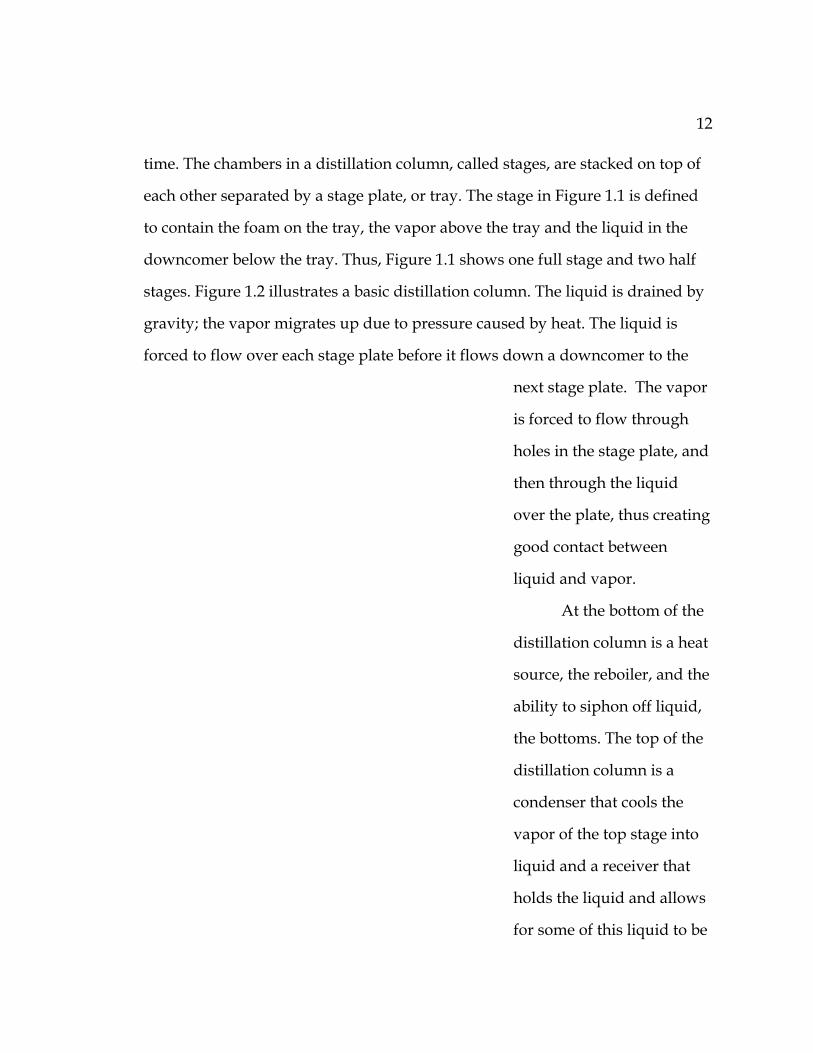
time. The chambers in a distillation column, called stages, are stacked on top of

each other separated by a stage plate, or tray. The stage in Figure 1.1 is defined

to contain the foam on the tray, the vapor above the tray and the liquid in the

downcomer below the tray. Thus, Figure 1.1 shows one full stage and two half

stages. Figure 1.2 illustrates a basic distillation column. The liquid is drained by

gravity; the vapor migrates up due to pressure caused by heat. The liquid is

forced to flow over each stage plate before it flows down a downcomer to the

next stage plate. The vapor

is forced to flow through

holes in the stage plate, and

then through the liquid

over the plate, thus creating

good contact between

liquid and vapor.

At the bottom of the

distillation column is a heat

source, the reboiler, and the

ability to siphon off liquid,

the bottoms. The top of the

distillation column is a

condenser that cools the

vapor of the top stage into

liquid and a receiver that

holds the liquid and allows

for some of this liquid to be

Condenser

DistillateAccumulator

Reflux

Reboiler

Bottoms

Feed

Figure 1.2. The basic distillation column.

13

returned, the reflux, and some to be taken away as distillate. Somewhere in the

middle of the column is the feed, where the original mixture to be separated is

introduced into the column. Here, vapor rising from below heats the mixture

such that vapor rising to the next stage has a higher percentage of the low-

boiling component (component A) than the original mixture. The liquid flowing

through the downcomer will have a higher percentage of the high-boiling

component (component B). If all has worked well, the distillate will be a nearly

pure component of the mixture, the component with the lowest boiling point.

The liquid flowing down from the top stage, although initially pure, captures

the high-boiling component in the vapor coming up by cooling the vapor.

In a multicomponent distillation, both the distillate and bottoms are

typically composed of several of the original components. The most volatile of

the components will not appear in the bottoms and the least volatile of the

components will not appear in the distillate. The component appearing in both

distillate and bottoms with the highest percentage in the distillate is called the

high key. Similarly, the component appearing in both distillate and bottoms

with highest percentage in the bottoms is the called the low key. Essentially, the

distillation column separates the mixture into the high key and more volatile

components and the low key and less volatile components.

A real distillation process can be complicated by many factors. There

might be many components. The component to be separated out has neither the

highest nor lowest boiling point. The phase equilibria may not be as simple as

presented above (e.g., in an azeotropic mixture, the equilibrium temperature at a

specific ratio of components can be lower than the lowest boiling point of any of

the pure components). The components may form multiple liquid phases. Real

14

distillation columns become complex in meeting the requirements. Feeds of

different mixtures can come in on several stages. Distillate and bottoms may be

reintroduced at various stages. Sidestreams can transport liquid or vapor off any

stage to become feeds on another stage or into another column. Heat can be

added or removed from any stage. Several distillation columns can be used in

series (e.g. azeotropic mixtures require more than one column). Heat integrated

columns allow heat flows between columns. Additional components such as

solvents, may be added to facilitate separation. The condenser may not totally

condense the vapor into liquid. A variety of control strategies may be used to

stabilize or optimize the process. Designers of columns must consider these

factors as well as deciding the number of plates, the type of plates (see [1] or [2]

for the choices), whether tray plates are used at all, whether additional

components should be added to facilitate separation, or whether a simple

chemical reaction should occur. The ideas presented in this thesis are hoped to

be basic enough and bond graphing powerful enough to be applied to any of the

possible configurations.

The purpose of a tray is to facilitate liquid and vapor interaction; this

purpose is also fulfilled by a packed column, in which trays are not used at all.

The column is filled, or packed, with irregularly shaped objects designed to

create continuous contact between liquid falling down and vapor rising. This

form of distillation column is gaining popularity in industry [3]. The non-

hydraulic equations are identical with a trayed column, except a stage is no

longer defined by stage plates. The form of the dynamic equations is modeled

intuitively by partial derivatives; approximating this by a series of differential

equations, as if it were a trayed column, makes sense. One notable difference

15

between a packed and trayed column is that the pressure differential is much

lower in a packed column; the hydraulic equations for a trayed column could

not be used. The equations for a packed column will not be discussed.

Complex distillation can lead to a variety of problems; some of these

problems must be anticipated when designing or modeling a column. Weeping

occurs when the liquid flows down through the holes in the plate, caused by

insufficient vapor flow [2]. Flooding occurs when the liquid flows up through

the plate, caused either by excessive vapor flow (entrainment flooding) or

excessive liquid buildup on the stage (downcomer flooding) [1, 4]. Entrainment

is either the carrying off of liquid with the vapor through the plate or the

carrying off of the vapor with the liquid through the downcomer. Other

problems include downcomer blocking, oscillations in the liquid holdup, and

instabilities in the operations of the column. These problems can occur in any

distillation column with the right provocation, although design and control

systems should be able to limit the likelihood. Properly modeling and

simulating a column should expose such problems.

1.2 The basics of bond graphs

A bond graph is a graphical description of a physical system that

preserves the computational and topological structure of the system. Each bond

represents the transport of energy as a pair of conjugate variables (effort and

flow) that multiply together to represent power. Thus, bond graphs show the

flow of power through a system. Table 1.1 lists several pairs of conjugate

variables.

16

Bonds (half arrows) originate and terminate at various types of elements,

depending on the physical system and the equations used to describe them. The

basic elements describe fundamental relationships between the variables that

are attached by a bond or by bonds. These basic elements are listed in Table 1.2.

As suggested by their definitions, only the 0-node and 1-node accept more than

one bond. These elements will not be sufficient to describe a distillation column;

new elements will be developed to reflect the equational forms of the distillation

effort (e) flow (f)

pressure volume flow temperature entropy flow

force velocity chemical potential molar flow

voltage current torque angular velocity

Table 1.1. The basic conjugate pairs.

symbol name equation 0 0-node ∑

∀i fi = 0

1 1-node ∑ ∀i

ei = 0

R Resistance e = R * f or f = e/R C Capacitance

(Compliance) f = C dedt

I Inductance (Inertia) e = I

dfdt

SF Flow Source f = given SE Effort Source e = given

Table 1.2. The basic nodes of a bond graph.

17

column model and of thermodynamic systems in general.

Bond graphing a system provides more than just a graphical mapping of

the system. Bond graphing inherently provides some system analysis, an easy

means of expanding the system, and modularity. Each bond is assigned one

causality stroke that appears at one end of the bond. The causality stroke

determines which equation (represented by an element) is used to solve for each

variable; the stroke is placed where the flow variable is calculated. Thus, a bond

graph can determine whether a system contains algebraic loops or structural

singularities. Adding an element to the system (e.g., a resistor, a chemical

reaction, a heat source) can be represented by adding an element and a bond to

the bond graph. The effect of such a new element on the system can be seen

immediately by the placement of the causality stroke. Pieces of bond graphs can

be grouped into subsystems and be represented by a new element. Hierarchical

bond graphs are thus modularized to describe large systems.

It is beyond the scope of this thesis to describe bond graphs in all details.

See [5], [6], or [7] for a comprehensive introduction to the subject of bond

graphs and their use. For a comprehensive bibliography of bond graphs, see [8].

Bond graphs have proven to be useful in describing mechanical and electrical

systems. Bond graphs also provide a framework for working with convection

and with thermodynamics [9, 10, 11, 12, 13]. The use of bond graphs in chemical

systems has been limited, however. Chemical systems should benefit from being

bond graphed. Later sections will discuss how bond graphs can be assembled to

represent a distillation column.

1.3 The assumptions of a distillation column

18

In forming a model for the distillation column, general assumptions

about the operation of a distillation column must be made. The assumptions a

model makes are the major distinctions between the models found in the

distillation literature. A complete set of dynamic equations would be of a

daunting size considering that a stage contains many forms of energy

transformations and that a distillation column or a set of columns can contain

hundreds of stages. Of course, simplifying assumptions are desirable in such a

complex apparatus. Early computer models required stringent simplifying

assumptions to run [14, 15, 16].

Typical assumptions deal with system constraints (i.e. the type of column

and components used), heat flow, hydraulics, and dynamic equilibrium.

Assumptions leading to the simplest set of equations that approximate the

behavior of a distillation column are used. Assumptions can be broken down

within these categories of assumptions.

System constraints: 1) The condenser may be a partial or total condenser;

2) The trays may be of several types and each requires separate models for

vapor flow through them; 3) Chemical reactions must be modeled if the

components react. Distillation mostly does not include components that react,

though some models do allow for chemical reaction [4, 17, 18]. The most general

models also allow sidestreams, feeds, and heat transfer on each stage, allowing

for a specific complex column to be modeled.

Heat flow: 1) The column is adiabatic, the only heat exchanges by

conduction that need be modeled are those in the condenser and reboiler; 2) The

thermal capacitance of the column metal is negligible. Both of these assumptions

are used by almost all distillation models.

19

Hydraulics: 1) Vapor holdup (of mass and energy) on each stage is

negligible. The molar holdup of the vapor is usually much less than the molar

holdup of the liquid, thus, the vapor holdup effects are considered small. This

also allows for a great simplification in the equations as seen in the next chapter.

Further, more stringent, assumptions can be made that simplify the model

greatly, such as 2) constant pressure or pressures throughout the column, 3)

constant liquid molar holdup, 4) constant liquid volume holdup, 5) constant

reflux flow, or 6) negligible hydraulic dynamics. These simplifying assumptions

are essentially the assumption of small perturbations from steady-state.

Dynamic equilibrium conditions are assumed to be reached between the

vapor and the liquid before leaving the stage, which requires the intensive

variables (i.e. pressure, temperature, chemical potential) of both vapor and

liquid to be equal. In the simple example of single-stage batch distillation,

equilibrium was reached over time before draining and lowering temperatures.

In a distillation column, continuous heat and mass exchange is assumed to

create a dynamic equilibrium. This is the assumption of perfect mixing of vapor

and liquid on the stage. The equations detailing the vapor-liquid equilibrium

(the steady-state flow between the phases resulting in equal chemical potentials)

have a large variety of assumptions that determine their complexity and

whether they form an algebraic loop. The assumption of vapor-liquid

equilibrium is typically relaxed by using Murphree efficiency.

The assumption of negligible hydraulic dynamics is common in the

literature. In making the model as simple as possible, the equations for pressure,

fluid flow, and vapor flow are omitted and values are assumed. Justification of

this comes from Levy, who showed that the (steady-state, algebraic) hydraulic

20

equations had little influence on the most influential modes, the smallest

eigenvalues of a distillation system [19]. The equations dealing with the vapor-

liquid equilibrium were shown to be the most influential. Thus, first or second

order approximations of the distillation column could leave out the hydraulic

dynamics [20]. Work by Tyreus, et. al. and Lagar, et. al. verified that the

eigenvalues most influenced by the (steady-state, algebraic) hydraulic equations

are independent from those due to the vapor-liquid equilibrium, but that

removing the hydraulic equations does not reduce the stiffness of the system

[21, 22]. The assumptions used reflect the aim of the model. If comprehensive

dynamics are to be included, the hydraulic equations must be included.

Assumptions will play a large part in determining the scope and

desirability of a distillation column model. The severe assumptions of steady-

state, neglected hydraulics, or small perturbation models will not be considered

as possibilities. Assumptions and the resultant equations will be dealt with on

an element by element basis in the next chapter.

21

2.0 THE ELEMENTS OF A DISTILLATION COLUMN

A complete dynamic model of a distillation column must include

material balance and flow, energy balance and flow, liquid to or from vapor

flow within a stage, temperature, pressure, and hydraulic dynamics, system

constraints, and chemical reactions. Together, these relationships can define the

operations of a distillation column, as well as many other chemical and

thermodynamic processes. For modeling reasons, these relationships can be

seen in terms of power balances. In terms of power flow, the relationships

become temperature and entropy flow, pressure and volume flow, and chemical

potential and molar flow. These relationships and any bond graphs associated

with them are derived as separate elements of a distillation column. This

chapter will discuss the equations that form the traditional model, their origins,

their possible variants, and how they might be reformed into bond graph

notation.

From these equations, three models of a distillation column will be

formed. Equations used in the model of Gallun will be noted with a G. The

equations used in the simple modification of Gallun's model will be noted with

an S. Equations that form a rigorous model that can be bond graphed will be

noted with an R.

2.1 Mass balance

There is an overall balance of mass. This simple statement is carried to

the stage level. The conservation of mass is described by the equation:

22

dMass dt = (rate of liquid coming in – rate of liquid leaving)

+ (rate of vapor coming in – rate of vapor leaving) (2-1)

Many forms of equation (2-1) can be and are developed, depending on the needs

of the rest of the model [4]. Only a few are considered here, with the emphasis

on the mass balance for each stage j. The liquid coming into each stage is mainly

from the downcomer of the previous stage, the vapor coming in is mainly

through the plate from the stage below. Other sources of flow can include the

feed stream which is generally a liquid that comes in on only a few of the stages.

Sidestreams can remove some of the vapor or liquid from a stage in the middle

of the column [1]. Entrainment, both liquid-in-vapor and vapor-in-liquid, can

also be included in the model [1, 2, 23]. This thesis will not consider sidestreams

or entrainment, but results presented here should allow their inclusion.

Consider the mass balance in terms of molar holdup, Mj , and molar flow

for stage j:

dMjdt = (Fj + Lj-1 – Lj) + (Vj+1 – Vj) (2-2)

The liquid component balance for component i uses molar fractions of liquid

(xji ) and vapor (yji ):

d(Mj xji)

dt = (fji + Lj-1 xj-1,i – Lj xji) + (Vj+1 yj+1,i – Vj yji) (2-3)

Notice the assumption implicit in equation (2-3). The vapor molar holdup of

each component is constant, even though the vapor molar fractions are assumed

to vary. The changes in total molar holdup can be attributed solely to the liquid

of the stage. This assumption is not correct, but because the molar content of the

stage is primarily in the liquid, it is often deemed a good assumption. The vapor

23

molar fractions are allowed to vary as functions of liquid molar fractions. This

assumption also allows for the great simplification of obtaining the liquid

holdup without explicitly needing to know the flow from liquid to or from the

vapor within a stage. The variable Vj now contains this piece of information

(LVj = Vj+1 – Vj ). The change in molar holdup of each component as a liquid

on a stage (uji ) becomes [24]:

dujidt = (fji + Lj-1 xj-1,i – Lj xji) + (Vj+1 yj+1,i – Vj yji) (2-4)GS

xji = uji

∑ ∀i

uji (2-5)GSR

An alternative form of equation (2-4) is derived from equations (2-2) and (2-3)

[25]:

dxjidt =

1Mj

[fji – Fj xji + Lj-1 (xj-1,i – xji) +

] Vj+1 (yj+1,i – xji) – Vj (yji – xji) (2-6)

A more rigorous form of equation (2-4) does not assume constant molar

vapor holdup (uvji ):

dujidt +

duvjidt = fji + Lj-1 xj-1,i – Lj xji + Vj+1 yj+1,i – Vj yji (2-7)R

dujidt = fji + Lj-1 xj-1,i – Lj xji – LVji (2-8)R

duvji

dt = Vj+1 yj+1,i – Vj yji + LVji (2-9)R

24

In this form, the vapor-liquid equilibrium equations (section 2.4) must provide

not the molar fractions yji , but the actual flow rates of a component from liquid

to vapor, LVji . Very few distillation models consider non-constant vapor

holdup [26].

Mass balance is described in a bond graph as a 0-node. Molar flow and

chemical potential form a conjugate pair. Equation (2-8) is shown in Figure 2.1

as a collection of inflowing and outflowing bonds. The stroke at the end of the

top left bond indicates that the mass-balance is solved for duji/dt at the 0-node.

Solving for the conjugate variable, chemical potential, presents a separate

problem.

2.2 Energy balance

There is an overall balance of energy. The energy balance equation

closely follows the mass balance equation.

d(Energy holdup) dt = rate of energy coming in – rate of energy leaving

0µ

f ji

L x j-1,ij-1

Ljx j

LV ji

dujidt

ji

Figure 2.1. Bond graph of liquid mass balance equation (2-8).

25

Except for the condenser and reboiler, the energy coming into or leaving a stage

is solely through convection. This takes into account the assumptions of

negligible thermal capacitance and an adiabatic column. The equation for the

internal energy holdup of a stage (Uj ) is similar to equation (2-7):

dUjdt =

⎝⎜⎜⎛

⎠⎟⎟⎞Uf

j + Lj-1 U

Lj-1

∑ ∀i

uj-1i –

Lj ULj

∑ ∀i

uji +

⎝⎜⎜⎛

⎠⎟⎟⎞

Vj+1 UV

j+1

∑ ∀i

uvj+1i –

Vj UVj

∑ ∀i

uvji

= dUL

jdt +

dUVj

dt (2-10)R

Using the assumption of negligible vapor energy holdup, this equation can be

simplified to assign all changes in the stage energy to the liquid.

The thermodynamic relationships for internal energy and enthalpy (H)

state:

dUdt = T

dSdt – P

dVdt + ∑

i=1

c µi

dnidt (2-11)

dHdt =

dUdt + P

dVdt (2-12)

Because the volume of a stage is constant, the change in internal energy of a

stage equals the change in enthalpy. Typically, models for distillation columns

focus on enthalpy; there are approximations of enthalpy that can be calculated

from pressure, temperature, and molar fractions.

One method uses virtual values of the partial molar enthalpies to

estimate the enthalpy of the vapor, and a differential equation for the enthalpy

of the liquid [4, 27, 28]. Ideal gas enthalpies are found through a polynomial

26

expansion of the temperature of known coefficients. The actual enthalpy is

found by adding to this the departure from ideal enthalpy, as predicted by an

equation of state. The virial equation of state is used to calculate the enthalpy

departure function for stage j (Ωj ).

HVji = HIdeal

ji + Ωj (2-13)G

Ωj = Pj ⎝

⎜⎛

⎠⎟⎞ 2 –

1ZZj

⎝⎜⎜⎛

⎠⎟⎟⎞Tj

Bmj

Tj – Bmj

( )2 ZZj – 1 (2-14)G

The partial derivative depends on the mixing functions used to determine the

second virial coefficient of the mixture, Bmj . The exact equations used for the

partial derivative (51 of them) can be found in Appendix B and the ‘engder’

macro of Appendix D. The equation for the liquid enthalpy becomes:

dHL

jdt = Hf

j + Lj-1 HL

j-1

∑ ∀i

uj-1i –

Lj HLj

∑ ∀i

uji + ∑

∀i vj+1i H

V j+1i – ∑

∀i vji H

Vji (2-15)GS

Note the assumption that the difference in the vapor enthalpy flow is credited

towards the liquid: the derivative of the enthalpy of the vapor is assumed zero.

Other methods of enthalpy calculation involve various equations of state

[29, 30]. Some models use an algebraic equation for the enthalpy balance [25].

Although this form has been shown to be valid [28], it has also been shown less

accurate [31].

In bond graph notation, energy and mass are automatically balanced:

these equations manifest themselves automatically as 0-nodes and 1-nodes.

Instead of dealing with energy or enthalpy in bulk, the components of

27

thermodynamic energy are considered. The following equations, equation (2-11)

restated for one component in a mixture and one form of the Gibbs-Duhem

equation, reveal the conjugate pairs that bond graphs look at:

dUidt = T

dSidt – P

dVidt + µi

dnidt (2-16)

Gibbs-Duhem: dµidt ni =

dPdt Vi –

dTdt Si (2-17)

The corresponding bond graphs contain two new nodes: Ui is a 3 input

capacitive element and E0 is essentially a 3 input 0-node. The use of these nodes

will be discussed in the next chapter.

2.3 Hydraulic (pressure and volume flow)

Of all the equations within a distillation column model, the hydraulic

equations are the most dependent on the geometry of a particular column, and

thus, the most variable. Various types of vapor holes, multiple-pass trays with

multiple downcomers, circular flow paths, splash baffles and calming zones

before the tray weir, slotted weirs, laminar flow baffles, and various packing

arrangements all require special equations to become modeled.

A comprehensive analysis of stage dynamics would have to include the

partial derivative continuity equation (Navier-Stokes equation) to adequately

U iT

dSi /dt dV i /dt

dni/d

t

P

µi

E0dT/dt dP/dt

dµi/d

t

Si V i

ni

Figure 2.2. Internal energy elements.

28

describe the interaction of pressure with fluid velocity, viscosity, surface

tension, and density of the vapor and liquid as they flow through each other.

Bond graphs can be used to describe the continuity equation in fluid flow [32,

33]. For simplicity, flow could be divided into regimes such as spray, froth,

emulsion, bubble, and foam. These regimes have been studied and empirical

functions created relating various hydrodynamic parameters for each regime

[2]. The distillation literature contains many searches for theory and empirical

data that accounts for the formation of foam and spray, the flow patterns that

form upon and effect the hydraulics of a distillation tray, and the prediction of

densities within the different regimes [34]. Yet, such a comprehensive model of

the stage plate would require more information about the components than is

readily available and contains more information than needed. The large number

of untested equations in this type of model suggests more research.

Pressure and volume flow will be determined using Bernoulli’s equation

[35, 36]:

pressure1 – pressure2 = 12 ρ (velocity2

2 – velocity12 )

+ ρ g (height2 – height1) (2-18)

Bernoulli’s equation is essentially balancing the kinetic and potential energy in a

flowing fluid. The assumptions used to derive it are constant density,

temperature, and molar fractions, as well as perfect transfer of energy (no

thermal loss) and steady-state flow. A more complete version of Bernoulli’s

equation balances more forms of energy and uses length as its dimension [37,

38] :

29

⎝⎜⎜⎛

⎠⎟⎟⎞

J U1 + z1 + P1

ρ1 g +

v12

2 g – ⎝⎜⎜⎛

⎠⎟⎟⎞

J U2 + z2 + P2

ρ2 g +

v22

2 g

= ∆hf + ∆h (2-19)

where J is a conversion factor from heat to mechanical energy and ∆h is the

external work added to the flow. The term ∆hf is the pressure drop (called head

loss when length is the dimension) due to friction. The head loss can be related

to velocity of foam (uf), length of flow path (lf), hydraulic radius (rh), and a

friction factor (f) [27]:

∆hf = f uf

2 lf 12 g rh (2-20)

The friction factor is related to the Reynolds number, and is therefore viscosity

based. In most instances, this factor is quite small compared to the kinetic and

potential energy terms.

Where models in the distillation literature have sought to include the

liquid flow through the downcomer and vapor flow through the stage,

Bernoulli’s equation is used. The nature of the derivation of Bernoulli’s equation

is evident by examining a more comprehensive equation of motion with mass,

velocity and forces.

d(m v)

dt = ∑F (2-21)

The equation as it stands is suited for a Lagrangian frame of moving solids. The

equation needs reforming to be used in a Eulerian fixed frame of flowing fluid,

pressure differences and volume flows. This is achieved by dividing each side of

30

equation (2-21) by area and recasting mass and velocity into density (ρ), volume

(V), cross-sectional area (A), and volume flow(Q):

1

A0

ddt⎝⎜⎛

⎠⎟⎞ ρ V Q

A = ∑P (2-22)

Assume equation (2-22) refers to a section of pipe with constant a volume and a

fluid with a constant density; only the volume flow and area are left within the

derivative. The sum of pressures in this equation is the sum of the pressures at

the input and output, the pressure caused by the fluid moving in a gravitational

field (potential energy), and any frictional loss pressures. Thus, equation (2-22)

becomes

ρ V

A0 A2 (Q• A – Q A• ) = P1 – P2 + ρ g (height1 – height2) – Pf (2-23)

The term A0 denotes the average cross-sectional area. When the derivative of

volume flow is zero, steady-state flow requires the pressure differential to be

constant, hence a constant average acceleration through the tube. Part of this

pressure differential can be caused by a change in the cross-sectional area of the

tube; this is the kinetic energy term of Bernoulli’s equation. The derivative of

area in equation (2-23) is better formed using the derivative of velocity,

acceleration.

Q = v A

Q• = v• A + v A• = 0

A• = – Av v• = –

A2

Q a (2-24)

The kinetic energy term is thus calculated as

31

– ρ V Q A•

A0 A2 = ρ ∆x a = PKE (2-25)

ddt PKE = ρ v a (2-25a)

where a is the average acceleration through the tube. Equation (2-25a) only

makes sense in the Lagrangian sense of a changing ∆x; in the Eulerian sense, the

derivative is zero. The actual tube may not be shaped to give a constant

acceleration through the tube, but the average acceleration will always be the

same as if the acceleration is constant. Acceleration is derived using the

traditional method of deriving kinetic energy [35]. The main assumption is

movement with constant acceleration.

a = constant acceleration

v2 = v1 + a t t = 1 a (v2 – v1)

x2 = x1 + v1t + 12 a t2 = x1 +

1 a v1 (v2 – v1) +

1 2 a (v2 – v1) 2

a = v2

2 – v12

2 ∆x =

Q2

2 ∆x ⎝⎜⎛

⎠⎟⎞1

A 22 –

1A1

2 (2-26)

As long as the volume flow is constant, the average acceleration of flow through

the tube will equal this constant acceleration. Combining equations (2-23), (2-

24), (2-26), a full expression of fluid flow in a tube is realized.

ρ V A0

2 Q• + ρ Q2

2 ⎝⎜⎛

⎠⎟⎞1

A 22 –

1A1

2

= P1 – P2 + ρ g (height1 – height2) – Pf (2-27)

Note that the kinetic energy term is of energy stored, not of energy lost. A true

energy loss term would change sign with a change in the direction of flow. The

second term in equation (2-27) is represented by a KE-element in Figure 2.3;

32

although it is essentially a resistive element as long as flow remains in one

direction, it should not be represented by an R-element [39, 40, 41]. The

potential energy term is also an expression of energy stored. The form of

equation (2-27) is that of an inertia with various other elements attached:

∆P + PKE = P1 – P2 + PPE – Pf (2-28)

∆P = I ddt Q =

ρ V A0

2 Q• (2-28a)

PKE = ρ ∆x a = ρ Q2

2 ⎝⎜⎛

⎠⎟⎞1

A 22 –

1A1

2 (2-28b)

PPE = ρ g (height1 – height2) (2-28c)

Thus, a bond graph of this equation, using volume flow as the flow variable and

pressure as the effort variable, would center around a 1-node as in Figure 2.3.

Note that the potential energy term is not modeled using an energy storage

element; any tube used is not likely to be so long as to experience a change in

gravitational acceleration. At steady-state, the volume flow and pressures

become constant, which converts equation (2-27) into Bernoulli’s equation.

1

I KE

P1 P2Q

PKE

PPE

²P

SE R

Pf

Figure 2.3. Bond graph of fluid flow, equation (2-28).

33

Although constant flow is a common assumption, the fluid flows in a distillation

column are not always subject to constant pressures. Also, this assumption will

lead to an algebraic loop in the vapor flow, depending on how pressure is

calculated.

The fluid flow within a distillation column can almost all be modeled

using fluid flow in a pipe, equation (2-23). The major difference is that within a

distillation column, the flows are not always subject to the constant volume

assumptions of tube flow. Hydraulic power flow is considered as the conjugate

pair of pressure and volume flow. Referring to Figure 2.4, the hydraulic flow

variables are the vapor flow from stage j (QVj ), the liquid flow over the weir

Figure 2.4 The hydraulic variables in a distillation column stage.

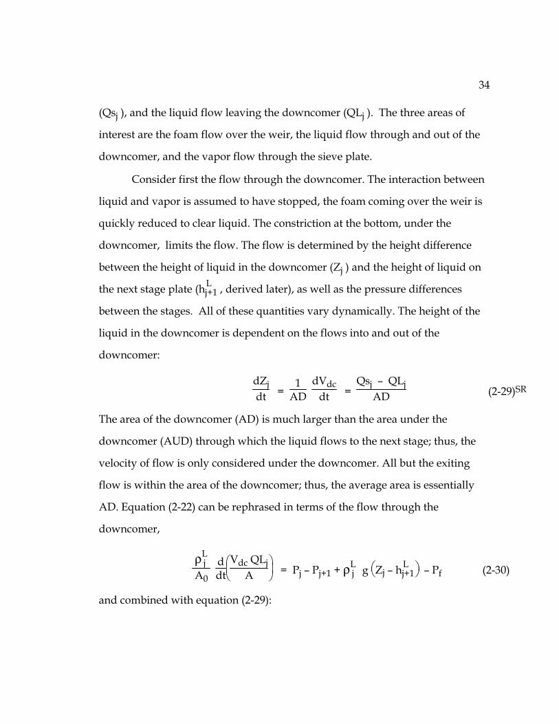
34

(Qsj ), and the liquid flow leaving the downcomer (QLj ). The three areas of

interest are the foam flow over the weir, the liquid flow through and out of the

downcomer, and the vapor flow through the sieve plate.

Consider first the flow through the downcomer. The interaction between

liquid and vapor is assumed to have stopped, the foam coming over the weir is

quickly reduced to clear liquid. The constriction at the bottom, under the

downcomer, limits the flow. The flow is determined by the height difference

between the height of liquid in the downcomer (Zj ) and the height of liquid on

the next stage plate (hL j+1 , derived later), as well as the pressure differences

between the stages. All of these quantities vary dynamically. The height of the

liquid in the downcomer is dependent on the flows into and out of the

downcomer:

dZjdt =

1AD

dVdcdt =

Qsj – QLjAD (2-29)SR

The area of the downcomer (AD) is much larger than the area under the

downcomer (AUD) through which the liquid flows to the next stage; thus, the

velocity of flow is only considered under the downcomer. All but the exiting

flow is within the area of the downcomer; thus, the average area is essentially

AD. Equation (2-22) can be rephrased in terms of the flow through the

downcomer,

ρL

j A0

ddt⎝⎜⎛

⎠⎟⎞Vdc QLj

A = Pj – Pj+1 + ρLj g ⎝⎛ ⎠⎞Zj – hL

j+1 – Pf (2-30)

and combined with equation (2-29):

35

ρA0

2 ⎝⎜⎛

⎠⎟⎞dQLj

dt Vdc + (Qsj – QLj) QLj + ρ QLj

2

2 ⎝⎜⎛

⎠⎟⎞1

AUDj2 –

1ADj

2

~= ρ ZjADj

dQLj

dt + ρ

ADj2 (Qsj – QLj) QLj +

ρ QLj2

2 AUDj2

= Pj – Pj+1 + ρ g (Zj – hL j+1 ) (2-31)SR

∆P = ρ ZjADj

dQLj

dt (2-31a)

PPE = ρ g (Zj – hL j+1 ) (2-31b)

Pdc = – ρ

ADj2 (Qsj – QLj) QLj + Pj (2-31c)

PKE = ρ QLj

2

2 AUDj2 (2-31d)

The kinetic energy term, equation (2-31d), should be immediately compensated

for (eliminated) by the expansion of the area through which the liquid flows

onto the next stage plate. Instead, the kinetic energy term is kept as an estimate

of resistance, as equation (2-20) for resistive head loss does not pertain here. The

DC

I R

Pj Pj+1

Qsj

PKE

PPE

²P

SE

Pdcj

QLj 1

Zj

QLj

Figure 2.5 Bond graph of downcomer hydraulics, equation (2-31).

36

bond graph of this equation, Figure 2.5, is quite similar to the bond graph of the

hydraulics of a tube, except the change in downcomer volume (dVdc) depends

on both the differences in volume flows and pressures. A new element is created

to implement this term. The thin arrowed line indicates that the DC element is

used to calculate Zj , equation (2-29), for the potential energy term.

Assuming that the potential energy considerations are the predominant

forces on the flow, essentially assuming constant flows, Bernoulli’s equation can

be used and the volume flow simplifies to

QLj = Cx AUD 2 g ⎝⎜⎜⎛

⎠⎟⎟⎞

Pj – Pj+1

g ρLj

– h Lj+1 + Zj (2-32)G

Note the inclusion of Cx, accounting for vena contracta effects. Flow through the

downcomer is often considered to have negligible dynamics and is omitted from

many models. The bond graph of equation (3-32) is similar to Figure 2.5 without

the I element or DC element.

For the flow over the weir, the most common equation used is Francis’s

weir formula, relating the height of foam over the weir (hfowj ) to foam volume

flow (Qfsj ), weir length (Lw), and a vena contracta factor (Cd) [2]:

hfowj = ⎝⎜⎛

⎠⎟⎞

3

2 Cd 2 g Qfsj Lw

23 (2-33)

The equation assumes the tray and the components are such that the full height

of foam on the tray is intact as the fluid flows over the weir (i.e., there is no

calming zone). Using relative froth density (φ), clear liquid flow (Qsj ) can be

solved for:

37

φ = ρL

j

ρfj =

hLj

hfj =

QsjQfsj

= howjhfowj

Qsj = 2 3 Cd Lw

2 g φ ( )howj

1.5 (2-34)

One modification found in the literature is to use a weir constriction factor (Fw)

and a foam factor (Foamj) and solve for the clear liquid height over the weir [1,

27]:

Foamj = hL

jhwj + howj

= φ + 1

2 = f(velocity of vapor)

howj = 1.426

g1/3 Fw ⎝⎜⎛

⎠⎟⎞

QsjLw

23 (2-35)GSR

The weir constriction factor modifies the effective weir length much the same as

Cd corrects for vena contracta effects. Francis’s weir equation or its modification

serves as the minimum hydraulics for some models [23, 42]. It can be derived

from Bernoulli’s equation [2]. Using equation (2-18), choose point 1 to be the top

of the foam in the middle of the column and point 2 to be a distance y down

from the top of the foam and just over the weir. The pressures are both equal to

the stage pressure. Assume the velocity at point 1 is much less than at point 2

and solve for velocity at point 2:

v2 = 2 g y

The velocity is only a function of depth. Note that at a depth of zero, there is no

liquid flowing over the weir. The differential volume flow becomes:

dQsj = dA v = Cd Lw dy 2 g y

38

which can be integrated from zero to hfowj to form equation (2-33). The

assumption of constant pressure acting on the foam flowing over the weir is

probably justified, unless the weir is short enough (as in a column of small

diameter) that the flow forms a seal above the downcomer.

In most cases, Francis’s formula is worth using. The only quantity to vary

dynamically is the height over the weir. The derivation of a dynamic equation

for the flow over the weir is similar to that of the flow through the downcomer.

Starting with equation (2-30), and using pertinent information for a tray,

ρLj AN

φ A02

⎝⎜⎛

⎠⎟⎞

hfj dQfsj

dt + Qfsj dhfowj

dt + ρL

j Qfs j2

2 φ [ ]Cd (hfowj + Lw) 2

= Pj – Pj+1 + ρ g y – Pf (2-36)

dQfsjdt =

1φ ⎝⎜⎛

⎠⎟⎞dQsj

dt – Qfsj dφ dt

The derivative of the height over the weir is not just the difference in volume

flows into and out of the tray, but must include the vapor to liquid flow and the

feed, as well as the dynamic relative froth density. The height over the weir can

be found rather simply as:

hfowj = hL

j

φ – hwj =

∑ ∀i

uji

_ρL

j

– AD Zj

AN φ – hwj

39

howj = hL

jFoamj

– hwj =

∑ ∀i

uji

_ρL

j

– AD Zj

AN Foamj – hwj (2-37)GSR

The derivative of the height over the weir is not as simple to find. Francis’s weir

formula will be assumed for use by the models developed.

In terms of bond graphs, the height over the weir represents the volume

of fluid on the tray plate. Rearranging equation (2-37) reveals the equation for

the tray volume.

Vtray = (howj + hwj ) AN =

∑ ∀i

uji

_ρL

j

– AD Zj

Foamj

Then the flow over the weir is a function of the tray volume. Equation (2-34) can

be then represented as in Figure 2.6a, by an effort source of gravity and

resistance of kinetic energy. What is not fully conveyed by this graph is that the

FwPj Pj

Qsj1Pj Pj

Qsj

SEPPE

PKE

R:KE

howj

Qsj

Figures 2.6a and 2.6b. Bond graphs of Francis weir formula, equation (2-34).

40

pressures of both these elements must be equal. The Fw element, shown in

Figure 2.6b, encompasses the effort source and the resistance.

Vapor flow through the plate depends on the type of plate. The equations

for a sieve tray are developed here. Equations for steady-state flow for bubble

cap and valve trays exist [1]. For a sieve plate, the vapor flow is through small

holes in the stage plate and is considered incompressible. The area of the holes is

significantly smaller than the total area of the plate. The vapor between the stage

below and the plate is considered to be well mixed and moving at a much lower

velocity. Using equation (2-27) as a starting point, the volume being considered

is the volume within the holes of the sieve plate, Vhj .

ρ Vj+1 Vhj

(Cvc AHj)2

dQVj+1dt +

ρ Vj+1 QVj+1

2

2 (Cvc AHj)2

= Pj+1 – (Pj + g ρLj h

Lj ) – g ρ V

j+1 LHj – Pf (2-38)

Vhj = AHj LHj

The stage plate is assumed thick enough that vena contracta effects (Cvc) are

determined within the holes. Rearranging for the derivative, and assuming the

vapor potential energy term to be negligible (i.e. LHj << hLj and ρ V

j+1 << ρLj ),

equation (2-38) becomes

dQVj+1

dt = Cvc2 AHj

ρ V j+1 LHj

⎝⎜⎜⎛

⎠⎟⎟⎞

Pj+1 – Pj – g ρLj h

Lj – Pf –

ρ Vj+1 QVj+1

2

2 (Cvc AHj)2 (2-39)SR

In this case, the pressure drop due to friction is related to the pressure needed to

create bubbles against surface tension (σ) with a diameter equal to the sieve

plate hole diameter (Dh) [2].

41

Pf = 4 σDh (2-40)

The assumption of constant forces allows Bernoulli’s equation to be used for

vapor flow from a stage. Also assuming that the frictional forces are negligible,

the vapor flow becomes,

QVj+1 = Cvc AHj 2

ρ Vj+1

⎝⎛ ⎠⎞Pj+1 – Pj – g ρLj h

Lj (2-41)G

The distillation models in the literature that include an equation for vapor flow

use equation (2-41). The bond graph of vapor flow, equation (2-39), is essentially

that of Figure 2.3.

The assumption behind the derivations of these hydraulic equations is

that pressure is being specified somewhere. An equation of state can be used for

pressure. Unfortunately, the equation of state is usually used to solve for other

variables, such as the molar density or compressibility factor. This, of course,

leads to algebraic loops. A full hydraulic bond graph of a distillation stage will

be developed in Section 3.1.

2.4 Vapor-liquid equilibrium (chemical potential and molar flow)

The equations related to vapor-liquid equilibrium are meant to predict

the flow of a component within a stage from vapor to liquid. The relationship

between the molar fraction in liquid (xi) and molar fraction in vapor (yi) is

generally not as simple as described in the example explaining distillation

(Section 1.1). Depending on the components and assumptions used, these

equations can form a large part of the model. This relationship is the most

important within the distillation column model. Levy, et al. showed that the

42

largest time-constants of a distillation model were due to composition dynamics

[19]. Ranzi, et al., found that up to 35% of the time in a distillation simulation

was taken by vapor-liquid equilibrium calculations [31]. The essential problem

of determining this flow is that chemical theory on this point is inadequate:

there are no equations for chemical resistance or chemical capacitance to relate

chemical potential and molar flow between the liquid and the vapor phases.

Instead of calculating the flow, the traditional method of determining

molar content is to assume that after good contact, vapor and liquid reach

equilibrium conditions. If equilibrium is assumed within a closed system with a

vapor phase and a liquid phase, there are no chemical reactions and pressure,

temperature, and especially the total Gibbs free energy are held constant:

dGdt = ∑

i=1

c

µLi

dnLi

dt + ∑ i=1

c

µVi

dnVi

dt = 0

In a closed system without reaction, it must also be true that molar flows are

equal and opposite:

dnL

idt = –

dnVi

dt (2-42)

Thus, the chemical potentials of a component in both liquid and vapor are equal:

µLi = µV

i (2-43)

This is the fundamental relationship used to predict multicomponent phase

equilibria [37].

Chemical potential is not used in the literature. What follows from

equation (2-42) is that at equilibrium, the fugacity of a component in a liquid

43

equals the fugacity of that component in vapor [4]. Fugacity of a component in a

mixture, fi , is defined for a constant temperature:

dµi = R T d⎝⎛

⎠⎞ln(fi) (2-44a)

limP∅0

fixi P

= 1 (2-44b)

If the mixture is a vapor, in an ideal mixture, and the ideal gas law holds, then

fugacity becomes the partial pressure of the component. This is evident from the

Gibbs-Duhem equation (2-17) combined with ideal mixture (the use of partial

pressure), constant temperature, and the ideal gas law.

(Gibbs-Duhem) dµidt ni =

dPidt V (2-45)

(Ideal Gas Law) V = ni R T

Pi

(Fugacity) dµidt =

R T Pi

dPidt = R T

d dt ln(Pi)

Essentially, the fugacity of a component is a measure of the partial pressure’s

deviation from Gibbs-Duhem and Dalton’s law (ideal mixture). Partial pressure

itself is still used in the traditional model, unqualified by deviations.

Measurement of the actual system pressure does not reveal fugacity, but

pressure. Chemical potential, which is not used in the traditional model, is

essentially absorbed into fugacity along with any deviations a component may

exhibit. In bond graph terminology, these equations suggest a transformer using

molar density as the transformation factor.

ni = _ρi V (2-46)

44

dµidt =

_ρi

dPidt =

_ρi

dfidt (2-47)

There are several ways to compute and approximate fugacity, depending

on the components used, each involving molar fractions. Thus, a relationship

between xi and yi is found by equating vapor and liquid fugacities. The general

equilibrium equation for this relationship can be stated as:

yi = Ki xi (2-48)GS

where Ki (referred to as the distribution coefficient [30] or K-value) can be a

simple or a complex function, depending on what approximations for fugacity

are used. The most basic expression for Ki, henceforth referred to as the ideal K-

value, is

KIi =

PSiP (2-49)S

where PSi is the vapor pressure (saturation pressure) of component i (a function

of temperature only), and P is the total pressure of the system. The ideal K-value

is the same as Raoult’s law:

P yi = PSi xi

This equation makes sense; for a pure substance, the equilibrium pressure for

two phases is, by definition, the vapor pressure. Thus, in a mixture, the partial

pressures of both liquid and vapor should be equal. If the vapor pressure of a

substance is twice the system pressure, then the vapor will have twice the molar

concentration of the liquid. The implication of this equation is that partial

pressure, not chemical potential, is driving molar flow between the phases. As

TMρ⎯

dµi/dtni

dPi/dtV

Figure 2.7 Transformer representing chemical to hydraulic power conversion.

45

may be expected, in mixtures, the partial pressures are not uniformly equal for

all substances and may serve as a poor model for molar flow. Hence, fugacity

has been introduced to replace partial pressures. Nevertheless, the essence of

these equations is based on the idea that a difference in partial pressure

(fugacity) is driving molar flow between the phases.

For a more detailed expansion, fugacity can be defined in terms of a

fugacity coefficient ϕi (measuring the deviation from partial pressure) , ideal

fugacity coefficient ϕi (measuring the deviation from pressure as a pure

component), activity coefficient γi (measuring the deviation from Dalton’s law),

ideal fugacity fi, ideal vapor pressure, and pressure [1, 4]:

f Li = γLi xi f

Li (2-50a)R

f Vi = ϕV i yi P (2-50b)R

f Li = PSi ϕLi (2-50c)R

If the substance forms an ideal gas and an ideal mixture and conforms to Gibbs-

Duhem, then the fugacity and activity coefficients are one and Raoult’s law can

be used. Combining these definitions, the relation between the molar fraction of

a component in vapor and in liquid can be calculated several ways:

yi = γL

i PSi ϕLi

ϕVi P

xi (2-51)

yi = γL

i KIi ϕ

Li

ϕVi

xi (2-52)G

Equations (2-51) and (2-52) are but the start of many various ways in which

molar fractions are calculated. Estimating fugacity and its coefficients occupies a

substantial segment of the chemical engineering literature. Some methods of

46

predicting

Error!

The method used by Gallun will serve as proper illustration [24]. Using

equation (2-51), we must come up with equations for PSi, ϕLi ,

ϕVi , and γL

i . The Antoine equation is used to calculate PSi:

log( PSi ) = Ai + Bi

T + Ci (2-53)GSR

where T is the only variable. Gallun’s equations used for ϕLi were taken from a

1967 monograph by Prausnitz, et al.

ϕLi = ϕS

i exp⎝⎜⎛

⎠⎟⎞

– αL

i PSiR T (2-54)GSR

ϕSi = exp( f1(TR) +ωi f2(TR) ) (2-55)GSR

Temperature is the only variable. To calculate

Error!

ZZ = 1 + Bm _ρ =

1 + 1 + 4 Bm P

R T2 =

P Vn R T (2-56)GR

Bm is the second virial coefficient of the mixture, which must be calculated using

the following mixing rules:

Bm = ∑i=1

c ∑ k=1

c yi yk Bik (2-57a)GR

Bik = R TCCik ( f3(TR) + ωHik f4(TR) + f4(µR,TR) + ηik f6(TR) )

PCCik (2-57b)GR

TR = T

TCCik (2-57c)GR

47

where the symbols here are constants or functions of yi and T [24]. Then

ϕVi can be calculated using the following:

ln⎝⎛

⎠⎞ϕV

i = 2 _ρV

∑ k=1

c yk Bik – ln(ZZ)(2-58)GR

Gallun uses the Wilson equation to calculate γLi . Again, the only system

variables that are present are molar fraction (xk) and temperature (T).

ln(γLi ) = 1 – ln

⎝⎜⎜⎛

⎠⎟⎟⎞

∑ m=1

c xm Λim – ∑

k=1

c

xk Λki

∑ m=1

c xm Λkm

(2-59a)GR

Λik = αL

k

αLi exp

⎝⎜⎛

⎠⎟⎞

– (λik – λii)

R T (2-59b)GR

αLi =

1_ρL

j

= f(T) (2-59c)GSR

Expanding these equations for all components for every stage, it is easy to

understand how these might form a significant portion of a model.

The problem of this method and all methods presented in the above

references are that equations for γLi involve xi and equations for

Error!

Another problem with using vapor-liquid equilibrium equations to find

the vapor molar fraction (yi ), is too many equations. Equation (2-48) and the

basic definition of molar fractions:

1 = ∑∀i

yi

48

form one more equation than is needed to find the values of the fractions. The

system is over-determined and generally is resolved by iterating the value of the

temperature until all equations are satisfied. A variation of this method is

presented in Section 2.5.

Currently, the only modification to equating liquid and vapor fugacities

is the use of an efficiency term. Several definitions have been proposed and

developed [2, 46, 47, 48, 49]. The vaporization and modified Murphree plate

efficiencies are defined as [4]:

Eji = f V

i

f Li =

yjiKji xji

(2-60)

EMji =

yji – yj+1iKji xji – yj+1i

= Eji –

yj+1iKji xji

1 – yj+1iKji xji

(2-61)

Ideally, the efficiency is one: the vapor and liquid fugacities are equal. Values

for modified Murphree efficiency are typically found empirically through some

estimate of plate dynamics, but can be derived using film theory, phase

resistances, and transfer units for steady-state flows [4]. One theoretical basis for

efficiencies is that chemical potential differences are driving molar flows

between phases. Using the definition of fugacity, chemical potential differences

are modified to become fugacity differences. Efficiencies are mostly used in

designing a column to discriminate between the number of ideal trays and

number of real trays that are needed.

49

2.5 Heat (temperature and entropy)

The conjugate pair for heat is entropy flow and temperature. Entropy is

not used in traditional models for distillation columns, there can be no bond

graph of these equations. Although there are tables of entropy values to be

found, they are not extensive enough in terms of substances covered, to be

useful. Instead, temperature is found through the over-determined set of vapor-

liquid equilibrium equations, described in Section 2.4. Otherwise, the dynamic

equation for temperature is typically derived from some function of

temperature and time, f(Tj,t):

ddt f(Tj,t) =

Tj f(Tj,t)

dTjdt (2-62)S

An appropriate function depends on the model. Because convection is the major

source of heat flow, the function should incorporate molar flow.

The dynamic equation for temperature can be derived from the vapor-

liquid equilibrium equation. Begin with the basic equations, sum over all i, and

then take the derivative:

yji = Kji xji

1 = ∑ i=1

c yji = ∑

i=1

c Kji xji

0 = ∑ i=1

c ⎝⎜⎛

⎠⎟⎞dKji

dt xji + Kji dxjidt (2-63)

If the ideal K-value is now assumed and the Antoine equation used, then K is a

function of Pj and Tj. The derivative of K can be stated:

50

dKjidt =

Kji

Tj dTjdt +

Kji

Pj dPjdt (2-64a)

Kji

Tj = Bi Kji ( )Tj – Ci -2 ln(10) (2-64b)

Now, let the derivative of Pj be zero, combine equations (2-63) and (2-64), and

solve for the derivative of Tj:

dTjdt = –

∑ i=1

c

Kji dxjidt

∑ i=1

c Bi Kji ( )Tj – Ci -2 ln(10) xji

Another function used is one for enthalpy, an approximation for enthalpy

in liquid as a polynomial function of temperature.

HLji = ai + bi Tj + ci T

2j (2-65)GS

Because the liquid enthalpy is calculated using a differential equation (2-15), the

derivative of Tj can be found similarly to the derivation above, without having

to assume a constant pressure. Again, the key here is that molar flow is the

assumed major conveyer of entropy.

Entropy is also flowing from the frictional loss terms of the hydraulic

equations, but this is not considered to be a significant source of heat. The real

heat flow by conduction occurs in the reboiler and condenser, which will be

dealt with in Sections 2.7 and 2.8.

2.6 Equation of state

51

An equation relating the steady-state pressure, temperature, volume and

number of moles is an equation of state. The equation can serve as a source of

behavior of a system. Usually, an equation of state is used to solve for the

system pressure of a stage. If the vapor molar holdup is assumed constant,

however, the molar volume (molar density) must be calculated from the

equation of state. Such a model usually uses Bernoulli’s equations to calculate

pressure and is forced to either assume values for liquid flow or use iterative

methods. The assumption of dynamic equilibrium means the pressure of liquid

and vapor are equal.

The equations of state considered are the ideal gas equation, the virial

equation of state, and the Peng-Robinson equation of state. Of these equations,

only the last one is valid for both liquid and vapor phases. Peng-Robinson does

assume that molar volume is known, it can not predict what percentage of the

substance is in which phase. Hundreds of equations of state exist [43]; these are

considered only as common examples. Also considered is a fluid that does not

change volume with a changing pressure, the incompressible fluid. Table 2.1

lists these equations of state. Which equation of state should be used will

Ideal P = RTv , v =

Vini

Virial P = R T Z

v , Z = 1 + Bv

Peng-Robinson P = RT

(v – b) – α a

v(v + b) + b(v – b)

α , a, b are functions of temperature, critical pressure and temperature, and the acentric factor

Incompressible v = a + b T + c T2

Table 2.1 Equations of state.

52

depend on the nature of the distillation components, as well as the information

available to compute constants within an equation of state. For instance, the

second virial coefficient (B) is detailed in equations (2-57).

Several capacitive relationships can be set up using these equations of

state, the internal energy equation and the Gibbs-Duhem equation. The

relationships are:

dSidt = Cs

dTdt (2-66)

Equation of State Cs = dSidt /

dTdt

Assuming

(All assume dUidt = 0)

Ideal µi niT2

dPdt =

dVidt = 0

PT dP

dt = dnidt = 0

Virial µi niT2

dZdt =

dPdt =

dVidt = 0

PT dZ

dt = dPdt =

dnidt = 0

Peng-Robinson µi RT(v – b)

ni

P

dPdt =

dVidt = 0

R v PVi(v – b)

ni

P

dPdt =

dnidt = 0

Pni

= v R T

(v – b)2 ni –

2 α a v (v + b)ni ( )v + ( 2 + 1) b 2 ( )v – ( 2 – 1) b 2

Incompressible – µi niVi T (b + 2 c T)

dPdt =

dVidt = 0

P niVi

(b + 2 c T) dPdt =

dnidt = 0

Table 2.2 Capacitance of Equation (2-66).

53

dVidt = Cv

dPdt (2-67)

dnidt = Cn

dµidt (2-68)

The relationships are only true under certain conditions. The values of Cs, Cv,

and Cn are shown in Tables 2.2, 2.3 and 2.4 along with the required conditions.

Note that none of these conditions are true in a dynamic distillation column. As

the equation of state is usually used for pressure calculation, equation (2-67) is

usually represented in a bond graph as a C element.

Equation of State Cv = dVidt /

dPdt Assuming

Ideal / Virial Vi2

ni R T dTdt =

dnidt = 0

Vi2 ⎝⎜⎛

⎠⎟⎞

1 – Si TVi P

Si T

dµidt =

dnidt = 0

Peng-Robinson v Vi R ⎝⎜⎛

⎠⎟⎞

1 – Si (v – b)

Vi RSi (v – b)

dµidt =

dnidt = 0

Incompressible Vi ni (b + 2 c T)

Si dµi

dt = 0

Table 2.3 Capacitance of Equation (2-67).

54

The value of Cn for the ideal gas equation is that used by Oster, et al. [50].

In describing the molar flow between phases, only the one for Peng-Robinson is

adequate in describing both phases. These relationships can only be used in

conjunction with equations that relate chemical potential to molar flow.

Unfortunately, as described in Section 2.4, no equations of state nor any other

equations exist to provide such a relationship. For instance, equation (2-68)

could be used to solve for chemical potential of both the liquid and the vapor in

a stage, based on the influx of total moles. The equation can not tell us the flow

between the phases because it is only valid for constant volumes. Nor would it

make sense to use such a storage element to describe phase flow.

2.7 Condenser and receiver

The condenser and the receiver are separate from the distillation column,

though essential for the distillation process. The condenser accepts the vapor

rising from the top stage plate and removes a significant amount of heat. The

main choice is between total and partial condensers, depending on the type of

modeling simplification desired. A total condenser is assumed to remove

Equation of State Cn = dnidt /

dµidt Assuming

Ideal ni

R T dVidt =

dTdt = 0

Virial ni

R T Z dZdt =

dVidt =

dTdt = 0

Peng-Robinson niVi

ni

P

dVidt =

dTdt = 0

Incompressible 1 dUidt =

dVidt =

dTdt = 0

Table 2.4 Capacitance of Equation (2-68).

55

enough heat to totally condense the vapor, that amount of heat varying with the

condition of the vapor flowing in. A partial condenser is assumed to remove a

fixed amount of heat, the amount of condensation varying with the condition of

the vapor flowing in. The thermal equations and the hydraulic equations

developed will be for a total condenser. No change in chemical potential is

assumed; phase changes are being driven by entropy flow.

The thermal aspect of the model is power flow due to convection,

conduction and heat of vaporization. The vapor is brought up against tubes

filled with cooling water. The amount of heat removed is controlled by the flow

of cooling water, which in turn is controlled by a valve. Conduction is a function

of thermal capacitance and thermal resistance. The thermal equations are of the

form,

heat flow = (volume flow) (heat capacity) (∆Temperature)

= (heat transfer film coefficient) (area of heat transfer) ∆T

change in heat holdup = (mass) (specific heat capacity) dTdt

The mass of the flowing cooling water, the mass of the vapor rising from the top

plate, and the mass of the condenser tubes must be considered in these

equations. Because total condensation is assumed, the desired variable is the

heat flow from vapor (QC). In the bond graph terminology of entropy flow, the

above forms can be converted [5].

entropy flow = (volume flow) (heat capacity) ∆T / T

= (heat transfer film coefficient) (area of heat transfer) ∆T / T

change in entropy holdup = (mass) (specific heat capacity) •T / T

56

Specifically, for the condenser described in the dissertation of Gallun [24], the

original heat flow equations are:

Ucw Ccw •T wo = Qcw Ccw (Twi - Two) + Uwm Aw (Tmc – Two)

(2-69a)GS

Umc Cmc •T mc = Uwm Aw (Tmc – Two) – QC (2-69b)GS

QC3 = [QV2]REF

QV2 Upmo Apc (Tj – Tmc)3 (2-69c)GS

The subscripts refer to cooling water (cw), water out (wo), water in (wi), and the

mass of the cooling tubes (mc). The equation for the heat flow from the vapor,

equation (2-69c), is an empirical approximation from reference values of vapor

and heat flow. Tj in this equation is considered to be some average temperature

between T1 (receiver temperature) and T2 (stage 2 temperature). Unlike pure

substances, the distillation mixture will not condense at just one temperature. In

terms of entropy flow, these equations become equations (2-70).

•S wi + ∆•S 1 = •S mc + •S wo (2-70a)R

•S mc + ∆•S 2 = QC/Tj + •S z1 (2-70b)R

•S wi = Qcw Ccw (Two – Twi) / Two (2-70c)R

∆•S 1 = Ucw Ccw •T wo / Two (2-70d)R

•S mc = Uwm Aw (Tmc – Two) / Two (2-70e)R

∆•S 2 = Umc Cmc •T mc / Tmc (2-70f)R

•S wo = Uwm Aw (Tmc – Two)2 / Two2 (2-70g)R

QC/Tj = Upmo Apc (Tj – Tmc)/Tj (2-70h)R

•S z1 = Upmo Apc (Tj – Tmc)2/(Tmc Tj) (2-70i)R

57

The equation for •S wo reflects the idea that the power lost in the resistance

between the cooling water and the condenser tubes is regained as heat flow into

the cooling water. The assumption that (Two >> (Tmc – Two)) effectively

eliminates this term from Gallun’s equations (2-69). Figure 2.8 shows the bond

graph associated with equations (2-70). The R element, equation (2-70a), in

contrast to the RS element, shows that power is lost to convection as the cooling

water flows away, and is modulated by the volume flow of cooling water, Qcw.

Knowing the heat loss (QC), the enthalpy-balance for the receiver becomes a

variation of equation (2-15):

dHL

1dt = –

L1 HL1

∑ ∀i

u1i + ∑

∀i v2i H

V 1+1i – QC (2-71)GS

The hydraulic aspect of the condenser is the volume flow of vapor

entering (QV) and the liquid flow leaving. The mass holdup in the condenser is

assumed to be constant and at temperatures that vary between T1 and T2. The

model assumes a weighted average of T1 and T2. The volume flow of vapor is

QC/T j10SE 1 0

RSR

C:cooling water

C: cooling tubes

Twi Two Two Tmc Tmc

²T Swi•

²S ²S

Swo

SmcSmc QC/T j

²T

Swi•

Swi•

Two Tmc

•

•

•

• •

RS

Sz1 ²T•

1Tj

Figure 2.8. The bond graph of the condenser, equations (2-70).

58

calculated using an empirical estimation based on pressure differences and the

vapor’s molar density. Also to be considered is the volume flow of cooling water

through the cooling tubes, Qcw. The pressures at the inlet and the outlet of these

tubes are considered constant and the flow is controlled by means of a valve.

Figure 2.9 reveals this simple system.

The hydraulic aspect of the receiver concerns pumps and valves. The

receiver is the chamber in which the condensed vapor resides before it gets

pumped out. An electric pump is a transformer of electric power to mechanical

power to hydraulic power [36]. This is shown in the bond graph of Figure 2.10.

The exact nature of the electric power being supplied depends on the pump. A

pump is essentially a flow modulated pressure source. Various equations for a

pump illustrate this aspect [24, 51]:

∆P = kpump Qmax – q (2-72a)R

∆P = a + b q + c q2 (2-72b)GS

1

R:valve

SE SEPw1 Pw3

²P Qcw

Figure 2.9. Cooling water flow in condenser.

TM TMe Γorque ²Pi ω Q

Figure 2.10. Bond graph of pump.

59

The form of these equations is of a negative resistor. A valve is a hydraulic

resistor used to control the flow of the fluid. Equations for a valve include [24,

51, 52]:

∆P = kvalve

2 A2 q2 (2-73a)R

∆P = a + b q + c q2 + d q3 (2-73b)GS

Combining pumps and valves is the essence of hydraulic flow out of the

receiver and the base of the column. Fluid flow from the receiver first goes

through a pump, then is split into two pipes each containing a control valve.

One pipe, containing the reflux, leads to the stage plate below and the other

pipe, containing the distillate, leads out of the system. This setup is best shown

using a bond graph, Figure 2.11. The effort source on the right is the

01

1

1

R:pump R:valve1

R:valve2

SEP1 Pd1 PD

P2

qr + qd q

q

Ppmp Pv1

Pv2SE

PPE

distillate

reflux

Figure 2.11. Bond graph of pump and valves below receiver.

1

R:pump&valves

P1qd + qr

²P

P2

SEPD

SEPPE

qd + qr

I

01

1

1

R:pump R:valve1

R:valve2

SEP1 Pd1 PD

P2

qd

qr

Ppmp Pv1

Pv2

I

²P

²P

SE

PPE

Figure 2.12. Bond graphs of pump and valves without an algebraic loop. a) Bond graph of pump and valves combined into one resistor. b) Bond graph

of pump and valves with inertial elements added.

60

pressure increase due to the vertical drop between the base liquid level and the

pump. The causality strokes can not be fully assigned because there is a choice

of assigning them. Hence, these equations form an algebraic loop. Two ways of

breaking this algebraic loop are to combine the resistances or

introduce other elements into the system. The valves can be seen as an

expression of Bernoulli’s equation (Figure 2.3) where there are only the resistive

element and the inertial element. Adding these inertial elements to Figure 2.11

will solve the algebraic loop, but this does require a knowledge of the physical

dimensions of the piping. The bond graph of Figure 2.11 can thus be solved

using bond graph Figure 2.12 a or b. The problem with joining the resistances is

that either PD and P2 must be joined somehow (by some average) or the flows

must be split somehow. There is no rigorous way to join non-linear resistors

along a Y-connection.

2.8 Reboiler

The reboiler infuses heat into and siphons fluid away from the distillation

column. The reboiler model is similar to the model for the condenser and

receiver. The base of the distillation column contains a pair of outlets; one

leading to the reboiler and one out of the system. The reboiler totally vaporizes

the fluid entering. Thermal conduction is the driving force of the vaporization.

The bottoms are taken out using a pump and valve in series.

The thermal aspects are essentially the same as the condenser. Tubes

filled with steam (the steam chamber) transfer heat into the fluid within the

reboiler until the fluid vaporizes. A complication exists in that the mass of steam

within the steam chamber is not constant because the steam is continually

61

condensing into water. This provides additional entropy flow from the heat of

vaporization. The thermal model for heat of vaporization is expressed in

equation (2-74):

Heat = m Lh = S T

Lh = a + b T (empirical estimate)

dHeat

dt = dSdt T =

dmdt (a + b T) (2-74)

If working in enthalpies (H) and tabulated estimates of enthalpies, the model

can be altered.

Lh = HV(Tsc) – hL(Tsc) (empirical estimate)

dHdt =

dmdt ( )HV(Tsc) – hL(Tsc) (2-75)GS

The steam flows from a steam header, which is under constant pressure,

through a steam valve, into the steam chamber. Within the steam chamber, the

phase change radically alters the volume flow by the change in density. The

water flows away under constant pressure. Hydraulically, the effect of the heat

of vaporization can be expressed as:

T

P

HOV

Qhov

Shov•

Figure 2.13. HOV element.

62

Qhov = dmdt

⎝⎜⎛

⎠⎟⎞1

ρV – 1

ρL (2-76)R

Because the liquid is usually much denser than the vapor, its term can be

reasonably dropped from equation (2-76). Together, these equations express a

link between thermal and hydraulic power that can be expressed as the HOV

element, shown in Figure 2.13. If the HOV element is to behave as other

elements, the power in equals the power out:

Qhov P = •S hov T

This presents more equations than is evidently needed to determine the flow

variables. The problem with these equations are that the chemical power has not

been accounted for. A third bond emanates from the HOV element supplying

chemical power to the process of condensing. This model does not need to

evaluate chemical potential because mass flow is determined by assuming the

steam chamber is filled with a constant volume of steam and a constant volume

of liquid. Thus, the mass flow of phase change from vapor to liquid is equal to

the mass flow into the chamber (Qsh ρsh). The HOV element presented here is

based on certain assumptions that do not exist elsewhere in the column: the

phase change is due entirely to heat loss and that heat loss is entirely conducted

away to the reboiler tubes. Mass flow and chemical potential are not directly

calculated or accounted for.

The reboiler and part of the base are shown in the bond graph of Figure

2.14. The entropy flows from the steam header into the steam chamber to the

metal of the tubes and into the reboiler chamber. The reboiler chamber is

considered to effect the entire base, and so the rightmost 0-nodes of Figure 2.14

show only some of the required bonds. Not shown are the effects of the liquid

63

and the vapor leaving or coming into the base. Unlike the other valves in the

system, the steam valve is modeled as an RS element, rather than just an R

element. All valves could be modeled as RS elements, but the hydraulic power

flow into thermal power is usually considered negligible. The INC element

assumes that the pressure is high enough (as would be typical in a steam

header) that the density of the steam

64

is not dependent on pressure, but on temperature alone. If the steam were not

considered incompressible, the INC element would be replaced by a C element

SESE

1 RS:

valv

e

0

10

SE: s

team

he

ader

R

Tsh

Tsc

²T ²P

PSH

Swo

Ssh

Qsc

Qsh

••

HO

V

²Q

Shov

•

RS

RS

11

00

C: s

team

ch

ambe

rC

: reb

oile

r tu

bes

²S1

²S2

Sx1

Sx2

TN

Tmr

QR

/TN

Smr

•

••

••

Tsc

²T²T

Tmr

0

PN

HO

V

²Q

Shov

•C

: R

eboi

ler

²S1•T

N

SVou

t•

INC

Qst

ore

V

Sx0

•

Psc

Figure 2.14. Thermal and hydraulic bond graph of reboiler.

65

(and the pressure could not be held constant by an effort source). The equations

related to Figure 2.14 are presented here as equations (2-77).

R: •S wo = Qsc Cwo (Tsc – Tsh) / Tsc (2-77a)R

Cwo = ρw hLsc

T (2-77b)R

RS: valve •S sh = Qsh Csh (Tsh – Tsc)/ Tsc (2-77c)R

•S x0 = Qsh Csh (Tsh – Tsc)2

Tsc2 + Qsh (PSH – Psc)

Tsc (2-77d)R

Qsh = f(PSH – Psc) (2-77e)R

HOV: •S hov = Qsh ρsh

Tsc (HVsc(Tsc) – hLsc(Tsc)) (2-77f)R

∆Q = Qsh ρsh 1

ρsc (2-77g)R

C: steam chamber •T sc = ∆•S1 TscVr Csc (2-77h)R

Csc = ρscT

HVsc + ρsc HVsc

T (2-77i)R

INC: QV store = Vrρsc

ρscT

•T sc (2-77j)R

RS: •S mr = Us As (Tmr – Tsc)

Tsc (2-77k)R

•S x1 = Us As (Tmr – Tsc)2

Tsc2 (2-77l)R

C: reboiler tubes •T mr = ∆•S2 Tmr

Umr Cmr (2-77m)R

RS: QR = Upmr Apmr (Tmr – TN) (2-77n)R

66

•S x2 = Uwm Aw (Tsc – TN)2 / TN2 (2-77o)R

HOV: •S hov = QLin ρL

TN ( )HV(TN) – hL(TN) (2-77p)R

∆Q = QLin ρL ⎝⎜⎛

⎠⎟⎞

1ρV –

1ρL (2-77q)R

The elements to the rightmost 0-node are only partially shown. The assumption

is that the entropy added to the liquid in the reboiler is added to the fluid in the

base itself. The enthalpy balance equation for the base becomes a variation of

equation (2-15):

dHL

Ndt =

LN-1 HLN-1

∑ ∀i

uN-1i –

LN H LN

∑ ∀i

uNi + QR – ∑

∀i vNi H

VNi (2-78)GS

The pipe under the base of the column also leads away from the system,

through a pump and a valve. Just as in the accumulator, the pump and valve in

series form an algebraic loop. Either the resistances can be joined or an inertial

element may be added to the valve. With only one valve and no Y-junction

1PN SE

SE

PPE

²P

R: pump & valve

PBQLN

Figure 2.15. Hydraulic bond graph of the base of the column.

67

splitting the flows, the solution is more straightforward. The “resistance” of the

pump and resistance of the valve can be joined directly, as shown in Figure 2.15.

The two effort sources represent the constant pressure of the bottoms’

destination (PB), and the pressure drop associated with the height of the liquid

in the base and in the pipe below the base.

2.9 Control system

Control of the distillation column can be effected by controlling the

valves. Controlling the valves effects the heat transfer and mass flow, as seen in

the previous bond graphs of the receiver, condenser, and reboiler. Flow,

temperature, and level measurement devices translate measurements into an

electrical current. The current is a signal that enters a PI controller. The control

signal coming out controls the valve position. To be modeled are the

measurement translation, the PI control, and the response of the valve to the

control signal.

The kth measurement translation is of the form

CIk = CImin + B Xk (2-79)GSR

where the constants, CImin and B, are set to translate a range of measurements

(Xk ) to a range of current values (CIk ). The PI control consists of comparing the

signal to a set point (CISPk ) at which the measured value is desired to reside,

and outputting a control signal if the signals are not identical.

ek = CIk – CISPk (2-80a)GSR

uk = Kpk ek + Kik ⌡⌠ek dt + e0 (2-80b)GSR

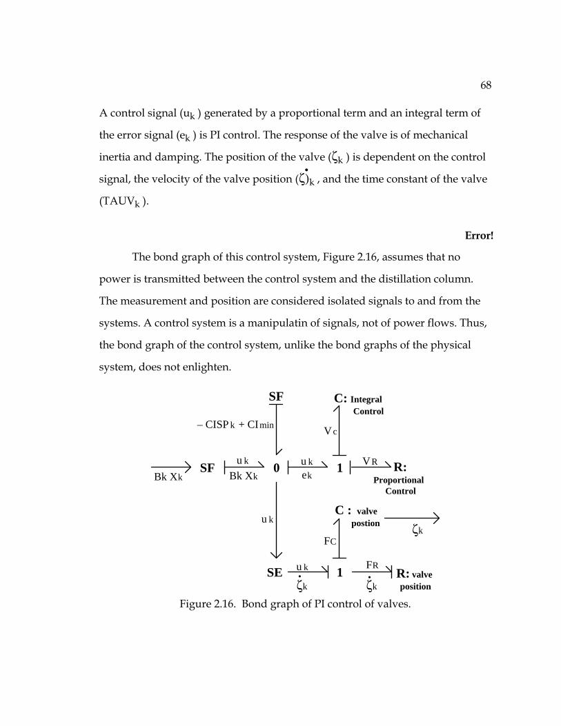
68

A control signal (uk ) generated by a proportional term and an integral term of

the error signal (ek ) is PI control. The response of the valve is of mechanical

inertia and damping. The position of the valve (ζk ) is dependent on the control

signal, the velocity of the valve position (•

ζ)k , and the time constant of the valve

(TAUVk ).

Error!

The bond graph of this control system, Figure 2.16, assumes that no

power is transmitted between the control system and the distillation column.

The measurement and position are considered isolated signals to and from the

systems. A control system is a manipulatin of signals, not of power flows. Thus,

the bond graph of the control system, unlike the bond graphs of the physical

system, does not enlighten.

0 1SF

SF

– CISP k + CImin

ek

C: Integral Control

R: Proportional

Control

1

C : valve postion

R: valve position

Vc

VR

ζk ζk

FC

FRu k

u k u k

SE

ζku k

Bk XkBk Xk

••

Figure 2.16. Bond graph of PI control of valves.

69

3.0 MODELING WITH BOND GRAPHS

Assembling the elements of a distillation column into a system is more

than just placing the equations together. The elements of a distillation column

interact dynamically. Bond graphs of the elements placed together will reveal

important aspects of the system. The traditional equations presented in the last

chapter were found to be deficient. Bond graphs point to a solution to this

deficiency.

3.1 Bond graph representation of the model

Thus far, the elements presented have closely followed the traditional

model of a distillation column. Bond graphs reveal the deficiencies that the

traditional model hides. Putting together the bond graphs of the previous

chapter and grouping them into hydraulic, chemical and thermal, three graphs

can be created. They are not complete. What has not been modeled traditionally

is the interface between the hydraulic, thermal, and chemical power at the point

of liquid and vapor flow interaction. Heat is flowing from the liquid to the

vapor in the form of heat of vaporization; heat is being convected along with the

fluid and phase flows; heat is being conducted back from the hotter vapor

(usually the hotter phase) to the cooler liquid. Chemical potential differences

(not pressure differences) are driving phase flow. Volume flow is being driven

by pressure and gravity, but is influenced by the source and sink of volumes

being generated and shrunk by the phase flow.

The traditional models of hydraulic, vapor-liquid equilibrium and

enthalpy balance do not need to present the nature of this interface. Using

70

equation (2-4) for mass-balance (with its assumption of negligible vapor

holdup), the phase flow need never be considered. The energy balance may then

be estimated by examining the assumed equilibrium results of phase flow. The

hydraulic equations need only be concerned with fluid flow beyond the phase

interaction.

The most concise bond graph representation of this traditional model is

using the convection bonds of Brown [53]. Figure 3.1 shows such a bond graph.

The convection bond combines the forms of power as one bond being driven by

molar flow. Entropy, temperature and chemical potential are combined into

intensive enthalpy. The VLE & Hydro element is a concise representation of the

possible models these equations may use. Depending on the precise model, this

element might be best represented by separate elements for the liquid and the

vapor flow. The Hydro portion of this element represents the hydraulic flow

apart from the vapor-liquid exchange. It could represent flow sources (constant

flow) or the entire scope of elements found in Section 2.3 (Figures 3.2 and 3.3

1

0

C

Pj, hji

nji•

vj+1i

vji

SF

f ji

VLE & Hydro

Pj-1, hj-1i

1lji l j-1i

Pj+1, hj+1i

L

Figure 3.1. Convection bond graph of distillation stage.

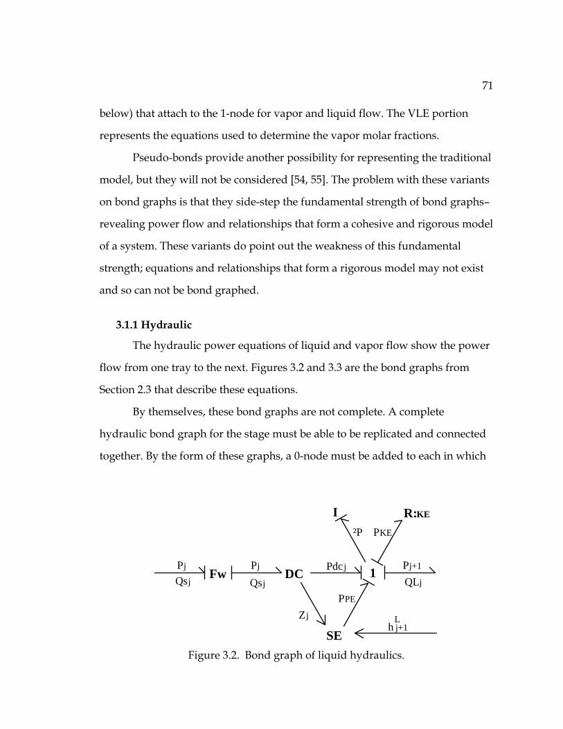
71

below) that attach to the 1-node for vapor and liquid flow. The VLE portion

represents the equations used to determine the vapor molar fractions.

Pseudo-bonds provide another possibility for representing the traditional

model, but they will not be considered [54, 55]. The problem with these variants

on bond graphs is that they side-step the fundamental strength of bond graphs–

revealing power flow and relationships that form a cohesive and rigorous model

of a system. These variants do point out the weakness of this fundamental

strength; equations and relationships that form a rigorous model may not exist

and so can not be bond graphed.

3.1.1 Hydraulic

The hydraulic power equations of liquid and vapor flow show the power

flow from one tray to the next. Figures 3.2 and 3.3 are the bond graphs from

Section 2.3 that describe these equations.

By themselves, these bond graphs are not complete. A complete

hydraulic bond graph for the stage must be able to be replicated and connected

together. By the form of these graphs, a 0-node must be added to each in which

1Fw DCPj Pj+1Pj

SE

I R:KE

Qsj QLj

PPE

PKE²P

Zj

Pdcj

h j+1L

Qsj

Figure 3.2. Bond graph of liquid hydraulics.

72

the pressure and the liquid

tray volume are calculated.

From what is known to be

happening on the tray, the

drastic density transformation

of phase change should also

be included.

Figure 3.4 shows a

possible bond graph configuration that attempts to meet this criteria. The

assumption here is that the pressures of liquid and vapor are identical. The

HOV element, just as in Section 2.8, attempts to explain the difference in liquid

and vapor volume flow. The volume flow is dependent on molar density and

1

I

SE

R:KE

QV j+1

PPEPKE

²P

Pj+1

Pj

Figure 3.3. Bond graph of vapor hydraulics

0 Qsji

0

0

QLj-1i

QV j+1i QV ji

QLpji

Pji

Pji

²Q ji

Cv :state

HOV

Vvapor•

QVp ji

Pji

SF

Qf

Figure 3.4. Expanded completion to hydraulic bond graph.

73

molar flow:

QLpji = LVji_ρL

j

(3-1a)R

QVpji = LVji_ρV

j

(3-1b)R

∆Qji = LVji ⎝⎜⎜⎛

⎠⎟⎟⎞1

_ρV

j

– 1

_ρL

j

(3-1c)R

= LVji ⎝⎜⎛

⎠⎟⎞R Tj

Pj –

1

_ρL

j

(ideal gas)

The HOV element does not relate pressure to volume flow, unless a state

equation is used for molar density. Figure 3.4 assumes pressure is calculated

with the state equation: the Cv element is the manifestation of a state equation

for vapor; see Table 2.3. Power flows out of the HOV element when the flow is

from vapor to liquid and into the HOV element when the flow is from liquid to

vapor.

Using the traditional method of determining molar flow requires using

fugacity. Fugacity can be assumed to be partial pressure, and so fall under the

auspices of hydraulics. Fugacity and volume flow may be conjugate variables,

but it is certainly not clear whether they form hydraulic power or can be

transformed (using a fugacity coefficient) to be joined to the rest of the hydraulic

bond graphs. Although it is reasonable to say that chemical potential differences

are driving molar flows between phases, fugacity differences will be assumed to

be driving volume flow. Efficiencies are essentially the inclusion of a molar flow

74

resistance. Figure 3.5 shows this additional resistance in which the vapor

volume flow is calculated. The exact nature of this resistance as a relation

between fugacity and volume flow

(or even molar flow) is unknown. The Fug element is used to calculate liquid

fugacity; the actual calculation does not express any relation between fugacity

and volume flow and so does not represent any real power flow. If the Peng-

Robinson equation of state is used, then the Fug element would be changed to a

Cv element. The fugacities are not identical to partial pressures and the Cv

element would need to be changed to adjust to a change in calculation.

Resistance alone may not be sufficient to describe dynamic vapor-liquid

0 HOV

1

0QV j+1i QV jifjiV

²f ji

Cv :state

R:efficiency

Vvapor•

0QLj-1i

QLpji

fji

²Q ji

QVp ji

fji

SF

QfL

ˆ

ˆ

ˆ

ˆQsji

L

FugQhov ji

Figure 3.5. Fugacity driven phase flow of traditional model.

75

flow. Instead, a form for dynamic equations can be assumed. The flow could be

modeled as a capacitive and a resistive element sharing a common molar flow:

d f Ci

dt = QVpji

C

QVpji = f C

i – f Li + f V

iR

except, the steady-state flow is now forced to be zero. Although this would

allow true chemical power to be used (Figure 2.7), this must be incorrect.

The flow could be instead modeled as an inductive and a resistive

element:

dQVpji

dt = f L

i – f Vi – f R

iL

f Ri = QVpji R

The transformation to chemical potential is not clear in this case. If fugacity is

considered as a variation on chemical potential (as it often is in the literature),

then the big assumption of this form is the existence of chemical potential

momentum. There is no theoretical basis for chemical potential momentum. If

fugacity is considered a variation on partial pressure (as this section has done),

then the assumption of this form is of pressure momentum (mass * velocity /

area). Conceptually, the nature of the velocity or area of the volume flow

between the phases is not clear at all. Essentially, this is the problem of phase

changes being driven by partial pressures. This form allows for the elimination

of a critical algebraic loop while preserving the extensive collection of

thermodynamic data contained in fugacity calculations that is already known.

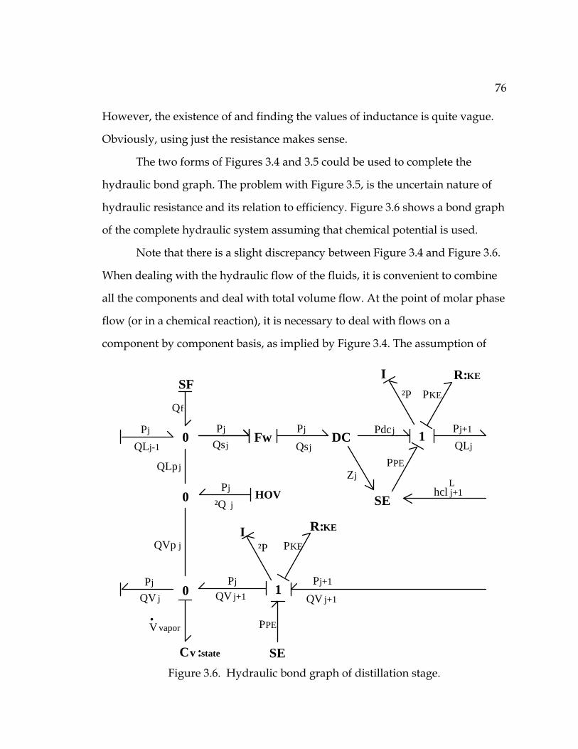
76

However, the existence of and finding the values of inductance is quite vague.

Obviously, using just the resistance makes sense.

The two forms of Figures 3.4 and 3.5 could be used to complete the

hydraulic bond graph. The problem with Figure 3.5, is the uncertain nature of

hydraulic resistance and its relation to efficiency. Figure 3.6 shows a bond graph

of the complete hydraulic system assuming that chemical potential is used.

Note that there is a slight discrepancy between Figure 3.4 and Figure 3.6.

When dealing with the hydraulic flow of the fluids, it is convenient to combine

all the components and deal with total volume flow. At the point of molar phase

flow (or in a chemical reaction), it is necessary to deal with flows on a

component by component basis, as implied by Figure 3.4. The assumption of

0 Qsj

0

0

QLj-1

QV j+1QV j

QLpj

Pj

Pj

²Q j

Cv :state

HOV

Vvapor•

QVp j

Pj

SF

Qf

1Fw DCPj Pj+1Pj

SE

I R:KE

Qsj QLj

PPE

PKE²P

Zj

Pdcj

hcl j+1L

1

I

SE

R:KE

QV j+1

PPE

PKE²P

Pj+1Pj

Figure 3.6. Hydraulic bond graph of distillation stage.

77

Figure 3.6 is that the volume flows computed at each component’s HOV element

can be simply added together to form the total volume flow. Unless the ideal

equation of state is used, it is also important to keep track of the molar fractions

to compute pressure (C element) properly.

Also note that the I elements are not necessary to eliminate an algebraic

loop. The assumption here is that the equation of state is used to solve for

pressure (the C element), the vapor molar density is found by a knowledge of

the vapor’s volume and molar holdup, and Zj is found using the DC element.

Otherwise, the elimination of the DC, C, and I elements (i.e., the use of the

equation of state for molar density in a traditional model) does involve the

hydraulic system in an algebraic loop.

3.1.2 Thermal

The traditional thermal and chemical equations for the distillation tray

are subsumed into the enthalpy equations. The thermal and chemical power

flow is assumed to be entirely dependent on convection outside of the vapor-

liquid interaction. Equilibrium conditions justify the use of approximations for

the enthalpy of the components.

There are three means of entropy flow between the phases. First, the

hotter phase (usually the vapor) conducts entropy to the cooler phase. Second,

entropy is convected with the molar flow between the phases. Convection is not

necessarily taking place in the same direction as conduction. Third, chemical

power and hydraulic power are combining to form the heat of vaporization into

or out of thermal power. Thermal power flow can be modeled. Figure 3.7 shows

a bond graph of entropy flow. Conduction is assumed to contribute very little

heat flow and is not modeled.

78

The C elements represent holdups of enthalpy in the liquid and the

vapor. The RS elements are modulated by volume or molar flow: they show

convection as the principle means of thermal power flow [5]. The exact

equations for these elements relate thermal resistance (R), specific thermal

capacitance (c), volume flow (q), and molar density (_ρ) :

C element: •Tj =

1C

•Shold =

⎝⎜⎛

⎠⎟⎞Tj

c n •Shold (3-2a)R

1 chemical and hydraulic power

1

0

HOV

1

RS

0 1

C

RSC

Shold• L

Sout• L

SdcL

²T

Tj+1

²T

SLV•

V

TjL

SxL•

SinV

SoutV•

Shold• V

Tj TjV V

²T

Sx• V

RS

0

RSSfeed•SETf

²T

TjL

•

Sxf•

Sx1•

Sx2•

SinL

TjL

0 Tj-1L

• •

Figure 3.7. Bond graph of thermal power flow.

79

RS element: •S L

dc = 1R ∆T =

⎝⎜⎛

⎠⎟⎞ C q

V ∆T = c q

_ρ

TL j-1

∆T(3-2b)R

•SL

x =

•S L

dc ∆TTj-1

= c q

_ρ (∆T)2

TL j-1

2 (3-2c)R

Equations (3-2b) and (3-2c) refer to the top right RS element. The volume flow in

this case is QLj-1 . Molar density is used, assuming compatible units for the

specific thermal capacitance. The other convection RS elements have similar

equations except the one associated with the molar flow. Instead of being

modulated by volume flow, molar flow should be used:

•SLV =

1R ∆T =

⎝⎜⎜⎛

⎠⎟⎟⎞

C LVji

nLVji

∆T = c LVji

T*j

∆T (3-3a)R

T*j =

⎩⎨⎧TV

j , LVji > 0

TLj , LVji < 0

(3-3b)R

•Sx1 = Error! (3-3c)R

•Sx2 = Error! (3-3d)R

Note that the entropy flows only in the direction of the molar flow.

The exchange of power flow due to heat of vaporization is not as well

defined. The model for heat of vaporization assumes a totally reversible process

at equilibrium conditions: the liquid and the vapor temperatures are identical

and non-varying. Replacing the central 1-node with a 0-node in Figure 3.7

would solve this problem, making the liquid and the vapor temperatures

identical, except that the thermal capacities of the liquid and the vapor phases of

a substance are not the same. Also, the distillation liquid and vapor might leave

80

the stage with almost the same temperature, after interacting, but certainly the

temperatures are different as they flow through each other. The form of the

known model can be described by the following equations.

Heat = n Lh = S T

Lh = a + b T (empirical estimate)

dHeat

dt = dSdt T =

dndt (a + b T) (3-4)

The heat flow is assumed into or out of the entire system. In a distillation stage,

the heat flow would presumably be into the vapor. The model is not adaptable

to two temperatures. Constant temperature would require the addition of

separate temperature regions between vapors and between liquids. The exact

nature of the relation between heat of vaporization, hydraulic power, and

chemical power is not defined. Thermal and hydraulic power flows from the

liquid to the HOV element and then towards the vapor (as thermal power)

when the molar flow is from liquid to vapor. Whether the power flow from the

liquid is partially thermal (conductive) or entirely chemical is unknown. Power

flows from the vapor (as thermal power) into the HOV element and then

towards the liquid (as chemical and hydraulic power) when the molar flow is

from vapor to liquid. Whether thermal (conductive) power flows to the vapor is

unknown.

3.1.3 Chemical

81

The theoretical inadequacies of the vapor-liquid equilibrium equations

have been addressed in the last chapter; they are based on pressure differences

rather than chemical potential differences. The only concession to non-

equilibrium conditions are efficiencies. Although efficiencies are essentially the

inclusion of a molar flow resistance, they do not relate molar flow to chemical

potential differences. The true resistance of flow is undoubtedly related to the

heat of vaporization as well as the power flow associated with the hydraulic

nature of the density transformation.

Assume a fixed-volume closed system of liquid and vapor. The chemical

0

thermal and hydraulic power

0

1 HOV

1

R

1

C

RC

n holdji• L

n outji• L

n inji• L

µjiL

² µji

µj+1i

² µi

jiV

µj+1iL

n injiV•

n outjiV •

n injiV

n holdji• V

µjiµjiVV

² µ

1R

n feedji•

SE

µfji

² µi

µjiL

•

n•LV

Figure 3.8. Chemical bond graph of distillation stage.

82

potential of the liquid is higher, so liquid evaporates. The pressure of the system

increases. In a traditional view of the system, the vapor pressure is higher than

the system pressure and liquid changes to vapor until the two pressures are

equal. Entropy flows into vapor as heat of vaporization as well as in convection.

The hydraulic power and thermal power can be expressed in terms of the molar

flow, but without an explicit relation to chemical potential, entropy flow or

pressure, the exact power exchange is unknown.

In terms of creating a theoretically appeasing bond graph, molar flow

would be driven by chemical potential differences in phase flow and volume

flow elsewhere. Figure 3.8 shows a theoretical bond graph of chemical power

flow in a distillation column stage. The R elements are expressions of convection

and so are modulated by volume flow.

R: •n = Cn q

V ∆µ

The form of the R elements is similar to the RS elements of the thermal bond

graph, Figure 3.7, except there is no chemical analog to specific thermal

capacitance. A better expression for the R element involves molar density:

R: •n = _ρj q (3-5)R

The C elements are of the form developed in Table 2.4. Equations (3-6) assumes

an ideal gas as well as the assumptions of Table 2.4, constant density and

temperature.

C: •µ = 1

Cn •nhold =

⎝⎜⎛

⎠⎟⎞ R T

n •nhold (3-6)R

83

Unfortunately, these assumptions are violated by the thermal and the hydraulic

C elements, and so equation (3-6) is not necessarily meaningful. The HOV

element is an expression of molar flow movement generated by the difference in

chemical potential. Its nature is explored in the next section.

3.1.4 Combining hydraulic, thermal, and chemical

The hydraulic, thermal, and chemical systems of a distillation stage are

linked. The capacitors of all three bond graphs (Figures 3-6, 3-7, and 3-8) are

linked. The hydraulic, thermal, and chemical power of the liquid and the vapor

is stored as internal energy. The equations become equations (3-7):

•UL

ji = •SL

ji TLji –

•VL

ji PLji + •n L

hold ji µLji (3-7a)

•UV

ji = •SV

ji TVji –

•VV

ji PVji + •n V

hold ji µVji (3-7b)

Hence, the capacitors are special types of the Ui element shown in Figure 2.2.

Unfortunately, internal energy on each stage is not held constant except at

steady-state and these equations do not add any required information.

The HOV elements of all three bond graphs (Figures 3.6, 3.7, and 3.8) are

linked. From the form of the power going in, it is tempting to use the same

equation for HOV element as the C element above; unfortunately this does not

make sense, as there is no substance to store energy. Also, the flows (through

variables) of each input are required to be determined from the HOV element.

The form of the HOV element is similar to the E0 element of Figure 2.2. The link

to the hydraulic and the thermal HOV elements requires that the molar flow be

determined from chemical potential differences. Assuming no holdup of energy

84

within the HOV element, then the chemical power should be as large as the sum

of thermal and hydraulic power, equation (3-8).

LVji = •S ∆T + P Qhovji

∆µji (3-8)

The problems with this equation are that the thermal power is not well defined

and that both the thermal power and the hydraulic power are dependent on

LVji . This equation will not work here. The exact relationship between molar

flow and chemical potential, although not known, can be hypothesized as a

resistance, similar to the hydraulic resistance based on efficiencies:

LVji = ∆µji

R (3-9)R

Unfortunately, the problem with efficiencies arises again; the value of this

chemical resistor is not known.

The third link between the systems is the thermal loss. Each of the

resistances in the hydraulic and the chemical bond represents power lost to heat.

For each R element in the hydraulic and chemical bond graphs, there exists an

RS element in the thermal bond graph into which the power flows; the power is

not lost. Equation (3-2c) specifies the introduction of this thermal power, and

assumes the chemical power and the hydraulic power loss to be negligible. This

equation, and all of the equations associated with RS elements, can be modified

to include this power.

•SL

x =

•S L

dc ∆T + •n Lout ∆µ + QLj PKE

Tj-1

85

= c QLj

_ρ (∆T)2

TL j-1

2 + QLj

_ρ (∆µ)2

R TL j-1

2 + ρ QLj

3

2 AUDj2 TL

j-1(3-2cmod)R

Thus, the joining together of the three systems into one bond graph can be

achieved by picturing only one HOV element, two C elements, and a limited

number of 0-nodes and 1-nodes. Figure 3.9 shows a distillation stage as a bond

graph. Note the extra 0-nodes; these are added for clarity and collapse with

other 0-nodes. The C, HOV, and RS elements represent links between the three

power bonds. The 0 and 1-nodes of Figure 3.9 do not link the three types of

power bonds, but link all the hydraulic bonds together, the thermal bonds

together, and the chemical bonds together.

86

C SF

RS

DCFw

1

0

0HOV

0 1

C

RS

1

SEI

RS1

SE

0

SEI

0

0

Figure 3.9. Bond graph of distillation stage.

87

3.2 Hierarchical bond graph representation

A full representation of a distillation column by bond graphs is as

daunting as the full representation by the system equations. The components of

a distillation tray are separable into three sections for the three areas of fluid

flow: the liquid off the tray, the vapor off the tray, and the fluid flow on the tray.

Each of these components can be broken down into their hydraulic, thermal,

and chemical aspects. Each of these aspects can be broken down into graphs for

each chemical component. Section 3.1 details the bond graphs

associated with each of these aspects. The complete bond graph, Figure 3.9,

obscures the possible differences that may arise with changing columns: various

equations of state, fugacity approximations, tray types, or downcomer

arrangements. Grouping bond graphs together into one element allows

hierarchical bond graphing, reducing the size and increasing intuitive

understanding of how the system works.

Figures 3.10, 3.11, and 3.12 show three hierarchical elements that are

created by grouping elements and bonds from Figure 3.9. The benefit of this

RS

1

SEI

0 Fluid

Figure 3.10. Bond graph of fluid flow represented by the Fluid element.

88

C

1

0

0HOV

0

C

Foam

Figure 3.11. Tray bond graph represented by the Foam element.

SF

1

SE

0

RSFeed

Figure 3.12. Bond graph associated with the feed represented by Feed element.

89

type of representation is that the new elements can be reformed into a new

representation of a distillation stage, Figure 3.13. The Feed element is not used

until Figure 3.17, but could have easily been included into the DCStage element.

In Figure 3.14, the Reboiler element is a representation of the bond graph of

Figure 2.14. Unlike the reboiler, the influence of the condenser in Figure 3.15 is

in more than just the transfer of thermal power. The

Condenser element is a representation of the bond graph of Figure 2.8. The

Pump & Valve(s) elements are representations of the pump and the valve

arrangements of Figures 2.12 and 2.15. Figure 3.17 brings together every

element. Because every connection of bonds is the triple bond of thermal,

chemical, and hydraulic, the hierarchical bond of Figure 3.15 is used to connect

Foam

Fluid

Fluid

Fw DC

DCStage

vapor entering

vapor leaving

liquid leaving

liquid entering

Figure 3.13. Distillation stage bond graph represented by the DCStage element.

90

the elements. Notice the similarity of Figure 3.17 and that of the drawing of a

distillation column, Figure 1.2.

Each element is not necessarily uniquely defined as shown in the

previous figures. The hydraulic aspect of a vapor flow, for instance is dependent

on the distillation tray used. The I element used in Figure 3.10 and defined by

equation (2-28a), applies to downcomers and sieve plates. Other types of

downcomers or plates may not require such an element or may require a

different definition. Although the internal structure of these elements may

Reboiler

QR/T N + Sx2•

Foam

Pump &Valve

0

SF: 0no vapor entering

DCBase

vapor leaving

liquid leaving column

liquid entering

Reboiler

Figure 3.14. Base and reboiler of Figures 2.14 and 2.15 represented by a DCBase element.

91

differ, the bonds coming out of these elements, if used, are well defined and

should not be changed.

Foam

SF:0 SF:0no vapor

leaving receiver

Pump &Valves

no vapor entering receiver

1

Condenser distillate leaving column

vapor entering condenser

reflux

Receivervapor

entering condenser

distillate leaving column

reflux

Condenser

1

Figure 3.15. Condenser and accumulator of Figures 2.9, 2.12, and 2.13.

Figure 3.16. Hierarchical bond.

92

0

DCStage

DCStage

DCStage

DCStage

Receiver

DCBase

Feed

• • •• • •• • •

Condenser

Reboiler

1

Figure 3.17. Hierarchical bond graph of a distillation column.

93

4.0 THE DISTILLATION COLUMN AS A SYSTEM

Models for distillation columns range from the simple to the complex.

Simple models provide the benefits of easy implementation, short run time, and

the possibility of design. Unfortunately, they also tend to be highly inaccurate in

their predictions of dynamic behavior (e.g. the start-up period of a column or

batch distillation where the contents of the feed changes). Many simple models

do not contain any differential equations, and are not solved using simulation.

Complex models have the benefits of being more accurate in their dynamics,

and thus more reliable in their predictions. Unfortunately, they are harder to

implement, take longer to complete a simulation run, are typically proprietary,

and contain so many component-dependent details that the full model is seldom

published. Complex models, taken as a system of equations, also can contain

algebraic loops that limit their usefulness. This chapter examines the historical

forms of the system of distillation equations. A specific example is also

considered and simulated.

4.1 The early models

The earliest model used in a systematic attempt to design distillation

columns was graphical. The McCabe-Thiele method uses a graph of the

equilibrium relationship of the component to be distilled, equation (2-48), to

determine the number of stages required and the proper reflux ratio [4]. The

assumptions of this model are enormous. The method is for designing columns

to separate binary mixtures with one feed and a simple equilibrium relationship.

94

Models for computer simulation purposes arose in the early 1960’s [14,

15]. The models concentrated on material-balance including simple equilibrium

equations. Meadows included enthalpy-balance equations [15]. Mah, et al.

admitted that the basic assumptions of distillation models were unrealistic

because of a lack of physical knowledge [14], hence the omission of enthalpy-

balance was seen as no great loss. Distefano introduced liquid and vapor flow

equations based on the mass-balance equations using the assumption of

constant liquid volume on each stage [16]. This model is still mentioned as being

a rigorous dynamic model by some [56]. Luyben presents the best aspects of

these models which serves as the basis for many models, using the assumption

of negligible vapor holdup, and obtaining the equations for mass-balance,

energy-balance, and dynamic equilibrium [57]. This base model is essentially

equations (2-4), (2-15), and (2-48). These three equations form many distillation

models [58, 59, 60, 61]. Hydraulic equations are omitted from these models, but

Van Winkle [1] and Lockett [2] have presented many empirical and theoretical

equations for fluid flow in a distillation column. Gani, et al. detail the modern

version of this model, including algebraic hydraulic equations and correlations

for column problems such as weeping [23]. Simulation of this model requires

the iteration of pressure and temperature.

Distillation is considered a mature field within chemical engineering,

much has been written on the subject, other models exist. Levy, et al. present a

model that does not fit the base Luyben model [19]. The model includes an

algebraic hydraulic equation for vapor flow, as well as an energy-balance

equation using heat capacities and heat of vaporizations, which can be solved

for temperature. A search of the literature failed to find this model being used

95

elsewhere. There are ‘rigorous’ simulation models that contain only algebraic

equations [62, 63]; there are models that attempt to reduce the number of

equations by grouping real distillation stages into fewer theoretical stages [64,

65]; there are models that emphasize the possibilities of controlling the

distillation process [66, 67, 68]. Today, many chemical system software packages

have the ability to design and/or simulate distillation columns [18, 68].

Unfortunately, the systems of equations used are most often proprietary, and so

can not be examined. For an extensive list of current distillation models and

distillation topics, see [69, 70].

The methods of simulating these models are various: backwards Euler,

Newton-Raphson, semi-implicit Runge-Kutta, Adams-Moulton (used in

conjunction with other methods), backwards-difference formulas, Gear’s

method. No purely explicit method can be used because of the algebraic loops

that the distillation column models contain [71, 72]. All of the models that

consider pressure a variable contain algebraic loops, also known as zero-order

causal paths or an index of nilpotency of one [73]. The best numeric method to

simulate such systems is Gear’s method [74]. A second problem encountered is

that chemical systems are typically stiff, the largest eigenvalues of the system

are much larger than the smallest eigenvalues. Stiff systems are not simulated

well using explicit techniques. Lagar, et. al. showed that the stiffness ratio for

distillation columns could be as high as one thousand [22]. Gear’s method, in

particular, simulates stiff systems well, making Gear’s method of integration the

preferred method in simulating chemical systems.

96

4.2 The Gallun model

The Gallun model is a complex model of a distillation column, based on

the Luyben model, developed by Steven Gallun and published in his

dissertation [24]. Not only are equations presented with details, but he

compliments this with details of his simulation technique and run. Although the

model is detailed, the equations presented are not complete. The complete

model, however, can be derived from later publications of his model [27, 28].

The Gallun model describes a 50 stage distillation column with complete

condenser, receiver, and reboiler that separates ethanol from a mixture of

ethanol, methanol, acetone, and water. There are three feeds and five control

valves that control the flow of various fluids. See Figure 4.1 for a diagram of this

column. Gallun assumes constant holdup of mass and energy in the vapor stage

of a model, allowing for mass and energy balance equations.

The hydraulic equations are derived from the Bernoulli equation for sieve

plates and downcomer, equations (2-32), (2-35), and (2-41). The first of these

equations is used to solve for liquid flow into the downcomer. Equation (2-35)

instead of equation (2-29) is used to solve for the height of the liquid in the

downcomer. The flow into and out of the downcomer is assumed identical, even

though the volume of the liquid is assumed to vary. The virial equation of state

is used to solve for molar density and the compressibility factor (used to

calculate fugacity). Pressure is solved for using the Bernoulli equation for vapor

flow, equation (2-41). The vapor flow is calculated using the fugacity equations

(vapor-liquid equilibrium equations).

97

Feed j = 3

j = 2

Feed j = 5

Feed j = 21

Distillate

Accumulator j = 1

Reflux

Pump 1

Total Condensers

cooling water

cooling water

control valve 1a

control valve 1b

control valve 2

control valve 3

Reboiler

Bottoms

Pump 2

Reboiler

j = 50steam in

steam out

steam in

steam out

control valve 4a

control valve 4b

control valve 5

Figure 4.1. The Gallun distillation column.

98

The vapor-liquid equilibrium equations are listed in equations (2-52)

through (2-59). Gallun avoids the over-determined system of these equations by

never solving for yji (except in stage one) . Instead, one modification is done to

equation (2-52) for stages 2 through 50:

yji = vji

∑ ∀i

vji (4-1)G

vji = γL

ji KIji ϕ

Lji

ϕ Vji

xji ∑ ∀i

vji(4-2)G

The new variable, vji , is the molar flow rate for component i leaving stage j as a

vapor. The sum of all vji is the total vapor molar flow rate leaving the stage, Vj ,

and equation (4-1) is certainly valid. These new equations pose a problem

besides introducing a new series of algebraic loops (pressure depends on vapor

flows depends on fugacities depends on pressure). In this model, there are four

components; equation (4-1) can be expanded thus:

⎣⎢⎢⎡

⎦⎥⎥⎤yj1 – 1 yj1 yj1 yj1

yj2 yj2 – 1 yj2 yj2

yj3 yj3 yj3 – 1 yj3

yj4 yj4 yj4 yj4 – 1

⎣⎢⎢⎡

⎦⎥⎥⎤ vj1

vj2

vj3

vj4

=

⎣⎢⎢⎡

⎦⎥⎥⎤

0

0

0

0

(4-3)

The form of this matrix is not particularly perverse until the determinate is

evaluated. The determinant of the square matrix is determined:

99

Det

⎣⎢⎢⎡

⎦⎥⎥⎤yj1 – 1 yj1 yj1 yj1

yj2 yj2 – 1 yj2 yj2

yj3 yj3 yj3 – 1 yj3

yj4 yj4 yj4 yj4 – 1

= 1 – yj1 – yj2 – yj3 – yj4 (4-4)

By the definition of molar fractions, the determinate must be zero. The solution

(the nullspace) is of the form:

⎣⎢⎢⎡

⎦⎥⎥⎤vj1

vj2

vj3

vj4

=

⎣⎢⎢⎡

⎦⎥⎥⎤y1/y4

y2/y4

y3/y4

1

(4-5)

This merely states that one of the vi’s is specified elsewhere before the others

can be found. The four variables are found through three independent

equations. These results make sense; for any concentration of a component,

there are an infinite set of rates at which this component might flow away. The

reason the equations work is that the system of equations is iterated to a

solution. There is only one set of rates that will give the correct concentration in

all fifty stages.

The first stage does use vapor molar fractions, there is no vapor flow

from the accumulator. Also, there are only 48 stage plates: Bernoulli’s equation

can only solve for 48 pressures. One other pressure is solved for using the

empirical estimate for flow through the condenser, equation (2-69c). The other

pressure is solved by iteration with the vapor-liquid equilibrium equations and

the equation of state.

Temperature is determined from the enthalpy balance. The method

described in Section 2.5, that of differentiating a function of temperature, is not

100

used. The differential equation for liquid enthalpy holdup is used, the

polynomial expansion of temperature estimation of liquid enthalpy holdup is

also used. This second equation is essentially solved for temperature by

iteration.

The column also includes a control system to ensure optimal

performance. Five control variables are controlled using the flow of fluid

through the five sets of valves in Figure 4.1. Four of the variables are the

temperature in the receiver (T1) controlled by flow of cooling water (Qcw)

through valve 1, the reflux flow rate (L1) controlled directly by valve 2, the level

of liquid in the receiver (Z1) controlled by the distillate flow through valve 3,

and the level of liquid in the base of the column (Z50) controlled by the bottoms

flow through valve 5. These four control variables use the PI control strategy

presented in Section 2.10, equations (2-79) through (2-81). The fifth controlled

variable, the temperature of the 35th stage (T35), is controlled by the flow of

steam (Qsh) through valve 4 using a cascaded PI control. For this control, the PI

equations are modified to be PI control for the valve, equations (4-6), where the

set point is determined by a PI control system of T35, equations (4-7):

CI4 = CImin + B Qsh (4-6a)GSR

e4 = CI4 – CISP4 (4-6b)GSR

u4 = Kp4 e4 + Ki4 ⌡⌠e4 dt + e0 (4-6c)GSR

•ζ4 =

u4 – ζ4 TAUV4

(4-6d)GSR

CI6 = CImin + B TM (4-7a)GSR

e6 = CI6 – CISP6 (4-7b)GSR

101

CISP4 = Kp6 e6 + Ki6 ⌡⌠e6 dt + e0 (4-7c)GSR

•TM =

T35 – TM TAUM (4-7d)GSR

Equation (4-7d) represents a temperature measurement device with first order

dynamics. The effect is to delay and dampen the effects of the actual

temperature on the control system. The effect of all of the equations (4-7) is to

delay and dampen the effects of the temperature on the control of the steam

valve. With 14 stages between T35 and Qsh, the delay within the control is

intended to anticipate the delay within the column.

4.3 Modifying the Gallun model

The Gallun model contains algebraic loops. Algebraic loops can be a

problem for simulating. The simulation program Gallun generated for his model

was written from scratch into FORTRAN, utilizing Gear’s method of

integration. Gear’s method contains within it a process of iteration to solve

algebraic loops. Gallun reported no problems with stability of his simulation

routine, though his model does contain dependent equations.

A rigorous elimination of some of the algebraic loops requires knowledge

of power flow in phase changes not yet known. Without such knowledge, the

loops may be eliminated in a non-rigorous way. Three modifications to Gallun’s

model will suffice to free the column model of algebraic loops. The hydraulic

equations can be made more exact by including the inertial elements and the

DC elements. This adds differential equations to the model needed to break the

algebraic loops in the liquid flow from the downcomer and allows vapor flow to

be calculated from hydraulic equations rather than vapor-liquid equilibrium

102

equations. Instead of pure Bernoulli’s equations, the equations developed in

Section 2.3 are used, equations (2-29), (2-31), (2-35), and (2-39). The flow over the

weir is not assumed to be the same as the flow out of the downcomer.

The virial equation of state is replaced with the ideal gas equation of

state. The virial equation of state is more accurate, but involves vapor molar

fractions. In turn, molar fractions depend on pressure, and pressure is found

using the equation of state. In Gallun's model, molar fractions depend on vapor

flow, vapor flow depends of fugacity, and fugacity requires molar fractions. A

more rigorous model would allow the vapor molar fractions and molar density

to be calculated from the vapor holdups of each component, as liquid molar

fractions are found. This algebraic loop can also be broken by using a simpler

equation of state. An additional result of this switch is the reduction in the

number of equations. The calculation of the second virial coefficient for a

mixture requires a few equations (61 per stage) and the enthalpy departure

function (Ω) requires a few more (52 per stage). These are all eliminated by

using the ideal gas equation. Molar density is now computed by assuming that

the total vapor molar holdup is constant and therefore specified.

The third modification for eliminating algebraic loops is the use of

Raoult’s law for the vapor-liquid equations. The vapor molar fractions are thus

calculated using liquid molar fractions, pressure, and vapor pressure. The use of

fugacity and activity coefficients is more accurate, but as long as these are used

to calculate the vapor molar fractions, algebraic loops cannot be avoided. A

more rigorous model would use chemical potential instead of using partial

pressures or fugacities to calculate molar flow between the phases and thus

103

allowing the virial equation of state to be used. The equations to calculate these

coefficients are eliminated (28 per stage).

Two models result from these three changes, a complex model and a

simplified model. The complex model incorporates the changes to the

hydraulics, includes a non-constant vapor holdup, and must assume a form of

resistance for molar flow between the phases. These changes eliminate all of the

algebraic loops within the column and retain the thermodynamic and the virial

equation calculations, at the expense of having to make up resistance values and

create a larger set of equations than Gallun’s model. The simplified model

incorporates the changes to the hydraulics, uses the ideal gas law, and uses

Raoult’s law for determining vapor molar fractions. These three changes to

Gallun’s model eliminate all of the algebraic loops and simplifies the model

considerably within the column. Several more algebraic loops exist in the

plumbing leading from the reboiler and the receiver. These are solved by

combining the resistances of the pump and the valves as described in Sections

2.7 and 2.8. The complex model includes hydraulic inertias, but the exact size

and lengths of the pipes are not given and can not be included with any

precision.

The last modification to the Gallun model was to reduce the number of

stages and feeds in the model. The full number of stages would have created a

simple model of about 750 differential equations with several thousand

algebraic equations. The number of stages was reduced to nine stages. As the

intention of this simulation was not to exactly duplicate the Gallun model

(which itself is not based on any real column), but to investigate the form of

distillation column models, this reduction was felt to be reasonable. The final

104

results of all the modifications is a simple distillation column model without

algebraic loops, containing 135 differential equations, 697 equations total.

The unmodified Gallun model was coded into the modeling language

DYMOLA. DYMOLA has the capability of creating an ACSL program (a

simulation language [75]) to simulate a model. Appendix B contains the

unmodified Gallun model as presented in his dissertation [24], as well as

including details presented in other sources [28, 27]. Appendix B also contains

the DYMOLA code for this model as well as DYMOLA’s assessment, including

a list of algebraic loops within the model.

The simple model was coded into DYMOLA. Debugging of the model

had to be conducted iteratively with simulation runs, and so, to facilitate the

process, the model was coded into ACSL using only three stages and finally into

nine. The nine stage simple model ACSL code is given in Appendix C. It was

intended to be recoded into DYMOLA and take advantage of the latest system

analysis functions within DYMOLA, but time constraints have not allowed for

this. The complex model was also coded into ACSL, but has not been simulated.

Appendix D contains the ACSL code for this model.

A third, more rigorous model could be fashioned out of Gallun’s model.

The bond graph model of a distillation column presented in the previous

chapter point to transforming the model into a balance of hydraulic, thermal,

and chemical powers. Only the hydraulic power balances have been

incorporated into the modified models above. The enthalpy balance equations

could be transformed to the thermal bond graph equations. Heat capacities of

these substances do exist in chemical tables. The transformation of the

105

thermodynamic calculations to chemical power balances is not as easily done.

Such a third model is left for future work.

4.4 Simulation results

Using fewer stages than the original Gallun model meant different

steady-state conditions. Assuming volume flows are about the same, the

pressure and the temperature differences between the condenser and the

reboiler are greatly reduced. Steady-state conditions were approximated based

on material balance equations. The model was first simulated to achieve true

steady-state conditions. After this relaxation, initial conditions and controller

set-points were modified to begin subsequent simulation runs at steady-state

values.

time (min)

Dis

tilla

te fl

ow (m

ol/m

in)

180

200

220

240

260

280

300

0 10 20 30 40 50 60 70 80 90

simple

Gallun

Figure 4.2. Comparison of the distillate flow of Gallun and simple model in

experiment one.

106

The stages in the simple model are not labeled one through nine. In

anticipation of expanding the model back to 50 stages, the receiver kept its label

1, the base kept its label 50, the feed stage kept its label 21, and the temperature

controlled stage kept its label 35. The nine stages were thus labeled, receiver to

base, 1, 2, 3, 4, 5, 21, 35, 49, and 50.

The simple model was simulated under several experiments. The

experiments concern changing the set-points of some of the control variables.

The original experiment by Gallun was to raise the set temperature of the 35th

stage up 5 degrees Rankine. Essentially, such experiments are designed to

optimize the settings of the control system, to test the response of the system.

time (min)

Tem

pera

ture

of s

tage

35

(°R

)

625

630

635

640

645

650

655

0 10 20 30 40 50 60 70 80 90

simple

Gallun

Figure 4.3. Comparison between the stage 35 temperature in Gallun and simple

model in experiment one.

107

Figures 4.2 through 4.6 show some of the results of this first experiment

on both the simple model and Gallun’s original simulation [24].

time (min)

Tem

pera

ture

(°R

)

590

600

610

620

630

640

650

660

670

680

0 15 30 45 60 75 90

T50

T35

T2

T1

Figure 4.4. Simple model temperature spread for experiment one.

Bottoms flow (gal/min)

Z50

(ft)

7.85

7.9

7.95

8

8.05

8.1

820 840 860 880 900 920 940 960

Figure 4.5. Control of base liquid level in simple model in experiment one.

108

Figure 4.2 shows the distillate flow responding to the change in CISP6 . Both the

Gallun model and the simple model show a dynamic response such that the

distillate flow is reduced by the change. The simple model reveals less

overshoot due to the reduced size of the column. Figure 4.3 shows the response

of T35 to the change in its set point. Note that in the simple model, only five

stages separate stage 1 and stage 35; the reduced temperature differences within

the simple model require that the set-point for T35 be much lower than the T35

set-point in the Gallun model. The Gallun model appears to be much less

oscillatory, although there is a common 10 minute cycle in the two models. The

oscillations can be attributed to the control constants, which are set for a 50-

stage column.

Figure 4.4 shows the temperature profile of the simple column, the

oscillations in T35 can be seen to be related to the immense temperature swings

Wsh (lb/min)

T35

(°R

)

641642

643644645646

647648649650

651

1500 1600 1700 1800 1900 2000 2100 2200 2300

Figure 4.6. Control of T35 using steam flow (Wsh) in the simple model in

experiment one.

109

in the base. Using a better control system, the rise in T50 would be more

gradual. Note how T1 and T2 both begin to swing higher at t=0, but that the

temperature control of T1 immediately tries to compensate.

Figure 4.5 shows the response of another controlled variable, the base

liquid level. Here, one can see that the control system slowly works its way to

keep the level at 8 feet. The steam flow in the reboiler, Wsh, is used to control

T35. When the set point is raised from 641.16 to 647.16 °R, Wsh increases to raise

T35 and decreases to lower T35. This control system, as seen in Figure 4.6, is not

as stable or efficient as the base level control.

The second and third experiments are to lower the reference temperature

for the 35th stage. As can be seen from Figure 4.7, simply lowering this

reference temperature produces an oscillatory system. Experiment three, to

determine the source of the instability, lowers the reference temperature as well

as adjusting the controller gain values for the temperature and the steam valve

time (min)

Tem

pera

ture

(°R

)

580

590

600

610

620

630

640

650

660

0 15 30 45 60 75 90

T50

T35

T1

Figure 4.7. Temperature profile of the simple model in experiment two.

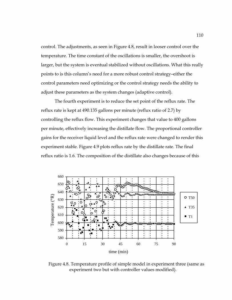
110

control. The adjustments, as seen in Figure 4.8, result in looser control over the

temperature. The time constant of the oscillations is smaller, the overshoot is

larger, but the system is eventual stabilized without oscillations. What this really

points to is this column’s need for a more robust control strategy–either the

control parameters need optimizing or the control strategy needs the ability to

adjust these parameters as the system changes (adaptive control).

The fourth experiment is to reduce the set point of the reflux rate. The

reflux rate is kept at 490.135 gallons per minute (reflux ratio of 2.7) by

controlling the reflux flow. This experiment changes that value to 400 gallons

per minute, effectively increasing the distillate flow. The proportional controller

gains for the receiver liquid level and the reflux rate were changed to render this

experiment stable. Figure 4.9 plots reflux rate by the distillate rate. The final

reflux ratio is 1.6. The composition of the distillate also changes because of this

time (min)

Tem

pera

ture

(°R

)

580

590

600

610

620

630

640

650

660

0 15 30 45 60 75 90

T50

T35

T1

Figure 4.8. Temperature profile of simple model in experiment three (same as experiment two but with controller values modified).

111

change. As seen in Figure 4.9, the

control brought the flow rate within .3 gallons/min. of the new set-point within

Distillate flow (gal/min)

Ref

lux

flow

(gal

/min

)

398.5398.7398.9399.1

399.3399.5399.7399.9400.1

400.3400.5

50 100 150 200 250 300 350 400

t=2

Figure 4.9. Reflux flow control in the simple model in experiment four.

Bottoms flow (gal/min)

Z50

(ft)

7.75

7.8

7.85

7.9

7.95

8

8.05

8.1

8.15

8.2

750 800 850 900 950

t=90

Figure 4.10. Base liquid height control in experiment four.

112

2 minutes. Obviously, controlling a flow rate directly using a valve results in

fast and efficient control. Figure 4.10 shows the base liquid level control

working; the bottoms rate reduces to compensate for the increased distillate

rate. Note that this experiment effects the level more than the first experiment,

Figure 4.5, where only the temperature needed changing.

The fifth and last experiment adjusted the composition of the feed,

without changing the temperature or total molar flow of the feed. The feed flow

of ethanol was increased as the feed flow of the other components were

decreased. Figure 4.11 shows the increase of ethanol in the bottoms product as a

result.

These five experiments verified the nature of the equations in the model.

Adjusting the various set-points did jolt the model in understandable ways,

consistent with the operation of a distillation column. However, the 9-stage

time (min)

mol

ar fr

actio

n (–

)

0

0.1

0.2

0.3

0.4

0.5

0.6

0.7

0.8

0 15 30 45 60 75 90

methanol

acetone

ethanol

water

Figure 4.11. Molar fractions of the bottoms product in the simple model with

experiment five (changing the composition of the feed).

113

model is not an adequate substitute for a full 50-stage model in several ways.

Most importantly, the simple model did not successfully distill ethanol. Nine

stages, one feed, simplified equilibrium equations, and control settings

established for a much larger column, combine to defeat the distillation goal.

One or more of these factors could possibly be optimized to achieve the proper

distillation, perhaps in future work. A fairer comparison to Gallun’s model

would increase the number of stages and feeds of the simple model.

114

5.0 CONCLUSION

Distillation columns provide a complex system to model. Previous efforts

to model distillation columns have focused on mass and energy balances, not on

power balances. These efforts require assumptions of equilibrium and constant

vapor holdup of mass and energy. For a rigorous dynamic model of the

distillation process, power flow reveals some inadequacies in these models.

Modeling using bond graphs have forced some questions about the nature of

distillation. The simple model shows that simple models can be constructed

without algebraic loops. The complex and bond graph model of the distillation

column show the potential in dynamic, rigorous simulation that can be

achieved. More needs to be done, both theoretically and in the fundamental

research of phase transfer, the basis of distillation.

5.1 Future work in distillation

Only the simplest modification of Gallun’s model was simulated. The

complex model needs to be simulated, possibly debugged. The simulation

results of the complex model will be hard to interpret. Multiple simulation runs

will be necessary to determine the role of the molar flow resistances and

hydraulic inertias. Both models need to be expanded to 50 stages and 3 feeds for

a proper comparison with Gallun’s model. These models should also be coded

into the modeling program, DYMOLA, to utilize the system analysis features it

currently contains. DYMOLA should be able to code an ACSL program that

simulates the model in a preordered, and therefore faster, sequence. Once the

115

power flow between the phases is better understood, a model based on the bond

graphs presented in this thesis can be constructed and simulated.

There are other methods of resolving the algebraic loops in Gallun’s

model. Differentiating the algebraic variables in a loop linearizes their

relationship; the loop is broken for these newly formed derivatives by linear

means of resolving algebraic loops. For such a large number of equations

involved within the algebraic loop of a distillation column, a systematic and

computerized application of this method must be applied. DYMOLA, has

recently gained the ability to render this, but has not yet been applied to the

distillation model. The potential benefit to the Gallun model is limited. The

bond graphing of the distillation column has revealed that the algebraic loops

are based on fundamental problems within the model.

Further work is needed on individual elements. The hydraulic resistances

(including valves) based on kinetic energy are suspect; viscosity plays no part in

these terms as they are currently defined. The vapor flow through the sieve

plate probably should not assume an incompressible fluid. The variety of

elements could be expanded to include the variety of distillation columns, such

as elements that describe fluid flow in a packed column. Work on elements will

mean adapting current forms of equations to power flows.

The bond graph model of a distillation column developed here, raises

many new elements and new questions. The most crucial question is the nature

of the molar flow between the phases. The energy-storage element of molar flow

and chemical potential needs work. The use of the Peng-Robinson equation of

state for a capacitive element, in conjunction with the phase resistances of film

theory could result in a viable set of dynamic equations for phase flow. The

116

problem is that efficiencies based on film theory are not considered to be very

accurate; empirically developed efficiencies work much better. These more

accurate efficiencies may themselves provide an adequate resistive element for

phase flow.

This thesis has tried to focus on macro power flow within a stage as

opposed to the micro power flows that sum up to these macro flows. A more

rigorous look at a distillation stage shows that pressure, temperature, and

chemical potential are not everywhere identical on each stage or within a phase

on each stage. The liquid pressure is dependent on the depth of the liquid. The

temperature of the vapor is dependent on how far it has traveled through the

liquid, the temperature of the liquid is dependent on the distance traveled

towards the weir as well as the depth of the liquid. The chemical potential

depends on the amount of phase flow already generated. All of these factors

affect the phase flow, density, and volume flow. Thus, a more rigorous model of

the distillation stage would need to take the form of partial differential

equations and, to be bond graphed, would be segmented into many areas of

exchange.

5.2 Future work in bond graphs

Bond graphs attempt to model a system using power flows under the

assumption that there exist fundamentally similar relationships between power

conjugates. The inherent power and weakness of this approach can be seen in

the scope of modeling a distillation column. The weakness of bond graphs is

that they do not adequately conform to the established forms of distillation

equations in use by current models. Modifications to bond graphs, such as

117

convection bonds, solve this problem, but at the expense of some of the inherent

power of the original bond graph. The inherent power of the bond graph is its

ability to graphically reveal the system, the ability to show the detailed form of

equations used, the ability to encapsulate pieces of the model into sub-models

using hierarchical bond graphs, and its demand for explicit details of the system

to adequately model the power flows in the system.

Bond graphs have shown some limitations to the traditional distillation

models. A choice of assigning causality strokes means algebraic loops within the

models. The algebraic loops point to fundamental problems within the system

equations. Some of these problems can be fixed immediately by including

additional elements, such as the hydraulic inertial elements. Some of these

problems can be solved in the type of relationship that is needed, but still

require a better understanding of the system, such as phase flow resistances.

The bond graphs also shows ways of expanding the model of a

distillation column presented. The addition of heat transfer or sidestreams

would expand upon the 0-nodes in the Foam element, similarly to the way the

Feed element does. A simple chemical reaction would mean the individual

components’ molar flow could not simply be added together. The 0-nodes in

Figure 3.2 would require an extra molar flow emanating from the node, the flow

of one component into another component as the reaction changes the chemical

makeup of the mixture. This would require the inclusion of a 1-node and one

ChR-element for each chemical reaction [5]. The 1-node connects individual

components that are involved in a chemical reaction. Figure 5.1 shows a

modification of the bond graph Figure 3.8 of a

118

distillation stage that includes liquid and vapor feed, liquid and vapor

sidestreams, a liquid heating element, and one chemical reaction that takes place

in the liquid.

C:liquid

DCFw

1

0

0HOV

0 Fluid

C:vapor

Fluid

Feed

0

0

Feed

1

ChR

Side

Side

Heat

Figure 5.1. A generalized distillation stage.

119

The strength of bond graphs–the demand for explicit details of the

system–is the major force behind the scope of future work that needs to be done.

The traditional model begins and ends with mass and energy balance. While the

traditional model has done very well emphasizing those known equations,

equilibrium estimates of enthalpy and fugacity, these equations only go so far. A

dynamic relationship between the variables in distillation is required for a

dynamic model. Bond graphs do balance mass and energy, and attempt to show

the dynamic flow of power, in all its forms. Bond graphs, I believe, show the

way of future pursuit. The chemical literature shows a lot of continuing interest

in developing better equilibrium models. Many chemical systems are stage

reactions and could benefit greatly from the modular aspects of bond graphs.

The true future of rigorous chemical systems modeling lies in developing loop-

free, dynamic, modular models, a future for which the bond graph methodology

is well suited.

120

APPENDIX A: NOTATION

A area

A0 average cross-sectional area

AD cross-sectional area of downcomer (constant)

AH total area of holes in the sieve plate (constant)

Ai, Bi, Ci coefficients that depend on component i

AN nominal area of stage plate (constant)

Apc area of heat transfer from condensing mixture to condenser

tubes (constant)

Apmr area for boiling heat transfer in the reboiler (constant)

As area for steam condensation in the reboiler steam chamber

(constant)

AUD area of opening under the downcomer, below downcomer

apron (constant)

Aw Area for heat transfer from cooling water to tubes (constant)

Bik second virial cross-coefficient of components i and k

Bmj second virial coefficient of the vapor mixture on stage j

C compliance element in bond graph

c number of components in mixture

Ccw cooling water heat capacity

CIk input to kth controller

CISPk set point (reference value) of kth controller

Cmc heat capacity of condenser tubes (constant)

Cmr heat capacity of reboiler tubes (constant)

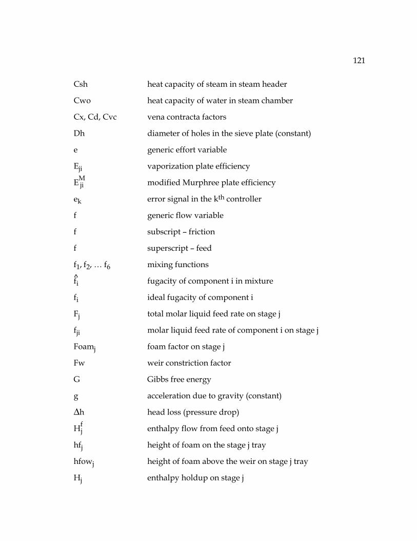
121

Csh heat capacity of steam in steam header

Cwo heat capacity of water in steam chamber

Cx, Cd, Cvc vena contracta factors

Dh diameter of holes in the sieve plate (constant)

e generic effort variable

Eji vaporization plate efficiency

EMji modified Murphree plate efficiency

ek error signal in the kth controller

f generic flow variable

f subscript – friction

f superscript – feed

f1, f2, … f6 mixing functions

fi fugacity of component i in mixture

fi ideal fugacity of component i

Fj total molar liquid feed rate on stage j

fji molar liquid feed rate of component i on stage j

Foamj foam factor on stage j

Fw weir constriction factor

G Gibbs free energy

g acceleration due to gravity (constant)

∆h head loss (pressure drop)

Hfj enthalpy flow from feed onto stage j

hfj height of foam on the stage j tray

hfowj height of foam above the weir on stage j tray

Hj enthalpy holdup on stage j

122

hLj height of clear liquid on the stage j tray

hLsc enthalpy of water in steam chamber (function of Tsc)

howj height of clear liquid above the weir on stage j tray

HVsc enthalpy of steam in steam chamber (function of Tsc)

hwj height of weir of stage j (constant)

I inertial element in bond graph

i subscript – denotes ith component of mixture

J conversion factor from heat to mechanical energy

j subscript – denotes jth stage

Ki K-value (distribution coefficient) of component i

KIi ideal K-value of component i

Kik integral constant of the kth PI controller

Kpk proportion constant of the kth PI controller

L superscript – liquid

Lh heat of vaporization per unit mass (function of temperature)

LHj length of holes in (thickness of) sieve plate of stage j

(constant)

Lj liquid molar flow rate from the jth distillation stage

lji liquid molar flow rate of the ith component from the jth

stage

LVji molar flow rate from liquid to vapor of component i on

stage j

Lw weir length (constant)

M molar holdup

123

N number of stages in distillation column, as a subscript it

denotes the base of the column

nji molar holdup of component i on stage j

P pressure

PB pressure outside distillation column to which bottoms flow

(constant)

PCCik cross-critical pressure of components i and k (constants)

PCi critical pressure of component i (constant)

PD pressure outside system to which distillate flows (constant)

Pdc pressure due to changes in the downcomer liquid height

Psc pressure in steam chamber of reboiler

PSH pressure in steam header (constant)

PSi ideal vapor pressure of component i (function of

temperature)

Q, q volume flow

QC heat flow from vapor into the condenser

Qcw volume flow of cooling water in condenser

Qfsj foam volume flow over the tray weir of stage j

QLj liquid volume flow leaving the downcomer of stage j

QR heat flow into liquid from the reboiler

Qsc volume flow of water leaving steam chamber

Qsh volume flow of steam from the steam header

Qsj liquid volume flow over the tray weir of stage j

QVj vapor volume flow from stage j

R ideal gas constant

124

R resistive element in bond graph

RS resistive-source element in bond graph

S entropy

SE effort source element in bond graph

SF flow source element in bond graph

T temperature

t time

TAUVk time constant of the kth control valve (constants)

TCCik cross-critical temperature of components i and k (constants)

TCi critical temperature of component i (constants)

TM temperature reading of measurement device used on stage

35

Tmc temperature of mass of cooling tubes in condenser

Tmr temperature of mass of reboiler tubes

TR reduced temperature (T/TC)

Tsc temperature of steam in steam chamber

Tsh temperature of steam in steam header (constant)

Twi temperature of cooling water coming into condenser tubes

Two temperature of cooling water leaving condenser tubes

Ucw mass of cooling water in condenser tubes

Ufj internal power flow from the feed on stage j

Uj internal energy holdup on stage j

uji molar liquid holdup of component i on stage j

uk output signal of the kth controller

Umc mass of condenser tubes (constant)

125

Umr mass of metal in the reboiler (constant)

Upmo reference heat transfer film coefficient between distillation

mixture and condenser tubes (constant)

Upmr boiling film coefficient in reboiler (constant)

Us reboiler steam side condensing film coefficient (constant)

uvji molar vapor holdup of component i on stage j

Uwm reference heat transfer film coefficient between cooling

water and condenser tube wall (constant)

V superscript – vapor

V volume

v velocity

Vdc volume of liquid in downcomer of stage j

Vhj Volume of holes in sieve plate of stage j (constant)

Vj vapor molar flow rate from stage j

vji vapor molar flow rate for component i from stage j

Vr volume of steam chamber (constant)

xi molar fraction of component i in liquid mixture

yi molar fraction of component i in vapor mixture

z height

Zj height of clear liquid in downcomer of stage j

ZN height of clear liquid in base of column, stage N

ZTj distance between stage plate j and stage plate j+1 (constant)

ZZj compressibility factor

α molar volume of mixture

126

α i molar volume of component i

γi activity coefficient of component i

ζk position of the kth control valve

ηik cross self-interaction parameters (constants)

λik – λii Wilson coefficients (constants)

µ chemical potential

µR mixture reduced dipole moment (constants)

ρ mass density

ρ_

molar density, moles per unit volume

σ surface tension

ϕi fugacity coefficient of component i in mixture

ϕi ideal fugacity coefficient of component i

φ relative froth density

ωHik cross-acentric factor of the first homograph of components i

and k (constants)

ωi acentric factor of component i (constant)

Ωj enthalpy departure function (from ideal gas) for stage j

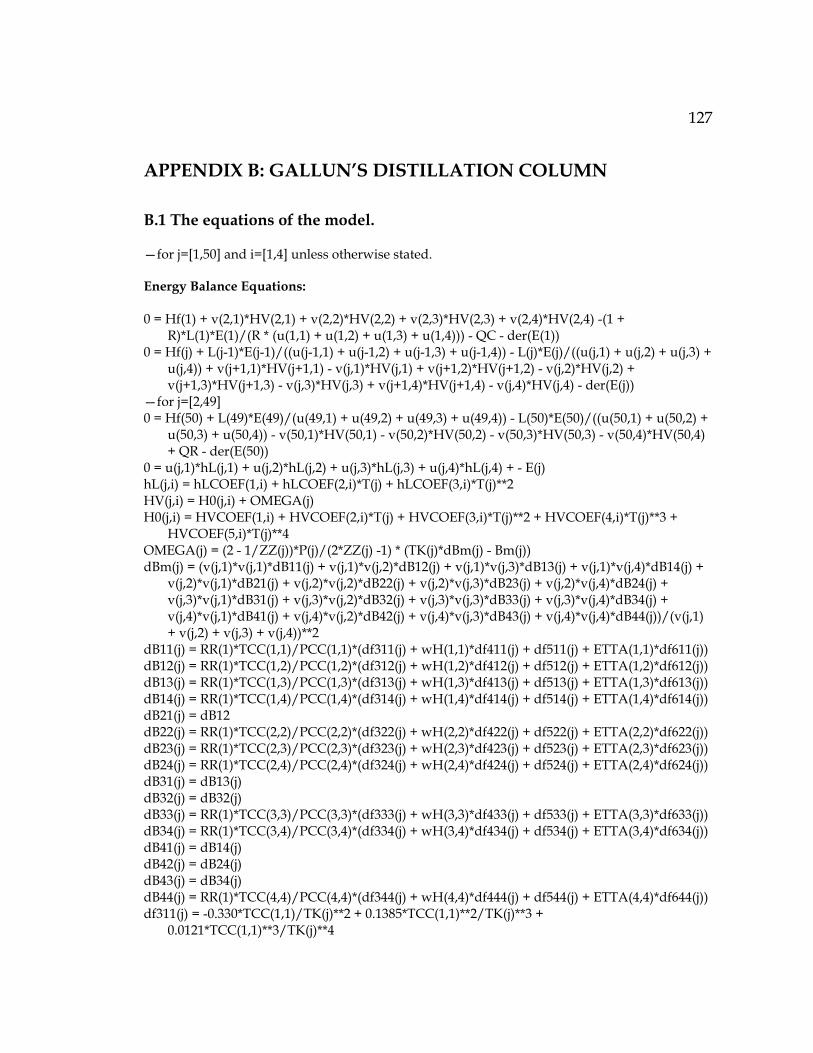
127

APPENDIX B: GALLUN’S DISTILLATION COLUMN

B.1 The equations of the model. —for j=[1,50] and i=[1,4] unless otherwise stated.

Energy Balance Equations: 0 = Hf(1) + v(2,1)*HV(2,1) + v(2,2)*HV(2,2) + v(2,3)*HV(2,3) + v(2,4)*HV(2,4) -(1 +

R)*L(1)*E(1)/(R * (u(1,1) + u(1,2) + u(1,3) + u(1,4))) - QC - der(E(1)) 0 = Hf(j) + L(j-1)*E(j-1)/((u(j-1,1) + u(j-1,2) + u(j-1,3) + u(j-1,4)) - L(j)*E(j)/((u(j,1) + u(j,2) + u(j,3) +

u(j,4)) + v(j+1,1)*HV(j+1,1) - v(j,1)*HV(j,1) + v(j+1,2)*HV(j+1,2) - v(j,2)*HV(j,2) + v(j+1,3)*HV(j+1,3) - v(j,3)*HV(j,3) + v(j+1,4)*HV(j+1,4) - v(j,4)*HV(j,4) - der(E(j))

—for j=[2,49] 0 = Hf(50) + L(49)*E(49)/(u(49,1) + u(49,2) + u(49,3) + u(49,4)) - L(50)*E(50)/((u(50,1) + u(50,2) +

u(50,3) + u(50,4)) - v(50,1)*HV(50,1) - v(50,2)*HV(50,2) - v(50,3)*HV(50,3) - v(50,4)*HV(50,4) + QR - der(E(50))

0 = u(j,1)*hL(j,1) + u(j,2)*hL(j,2) + u(j,3)*hL(j,3) + u(j,4)*hL(j,4) + - E(j) hL(j,i) = hLCOEF(1,i) + hLCOEF(2,i)*T(j) + hLCOEF(3,i)*T(j)**2 HV(j,i) = H0(j,i) + OMEGA(j) H0(j,i) = HVCOEF(1,i) + HVCOEF(2,i)*T(j) + HVCOEF(3,i)*T(j)**2 + HVCOEF(4,i)*T(j)**3 +

HVCOEF(5,i)*T(j)**4 OMEGA(j) = (2 - 1/ZZ(j))*P(j)/(2*ZZ(j) -1) * (TK(j)*dBm(j) - Bm(j)) dBm(j) = (v(j,1)*v(j,1)*dB11(j) + v(j,1)*v(j,2)*dB12(j) + v(j,1)*v(j,3)*dB13(j) + v(j,1)*v(j,4)*dB14(j) +

v(j,2)*v(j,1)*dB21(j) + v(j,2)*v(j,2)*dB22(j) + v(j,2)*v(j,3)*dB23(j) + v(j,2)*v(j,4)*dB24(j) + v(j,3)*v(j,1)*dB31(j) + v(j,3)*v(j,2)*dB32(j) + v(j,3)*v(j,3)*dB33(j) + v(j,3)*v(j,4)*dB34(j) + v(j,4)*v(j,1)*dB41(j) + v(j,4)*v(j,2)*dB42(j) + v(j,4)*v(j,3)*dB43(j) + v(j,4)*v(j,4)*dB44(j))/(v(j,1) + v(j,2) + v(j,3) + v(j,4))**2

dB11(j) = RR(1)*TCC(1,1)/PCC(1,1)*(df311(j) + wH(1,1)*df411(j) + df511(j) + ETTA(1,1)*df611(j)) dB12(j) = RR(1)*TCC(1,2)/PCC(1,2)*(df312(j) + wH(1,2)*df412(j) + df512(j) + ETTA(1,2)*df612(j)) dB13(j) = RR(1)*TCC(1,3)/PCC(1,3)*(df313(j) + wH(1,3)*df413(j) + df513(j) + ETTA(1,3)*df613(j)) dB14(j) = RR(1)*TCC(1,4)/PCC(1,4)*(df314(j) + wH(1,4)*df414(j) + df514(j) + ETTA(1,4)*df614(j)) dB21(j) = dB12 dB22(j) = RR(1)*TCC(2,2)/PCC(2,2)*(df322(j) + wH(2,2)*df422(j) + df522(j) + ETTA(2,2)*df622(j)) dB23(j) = RR(1)*TCC(2,3)/PCC(2,3)*(df323(j) + wH(2,3)*df423(j) + df523(j) + ETTA(2,3)*df623(j)) dB24(j) = RR(1)*TCC(2,4)/PCC(2,4)*(df324(j) + wH(2,4)*df424(j) + df524(j) + ETTA(2,4)*df624(j)) dB31(j) = dB13(j) dB32(j) = dB32(j) dB33(j) = RR(1)*TCC(3,3)/PCC(3,3)*(df333(j) + wH(3,3)*df433(j) + df533(j) + ETTA(3,3)*df633(j)) dB34(j) = RR(1)*TCC(3,4)/PCC(3,4)*(df334(j) + wH(3,4)*df434(j) + df534(j) + ETTA(3,4)*df634(j)) dB41(j) = dB14(j) dB42(j) = dB24(j) dB43(j) = dB34(j) dB44(j) = RR(1)*TCC(4,4)/PCC(4,4)*(df344(j) + wH(4,4)*df444(j) + df544(j) + ETTA(4,4)*df644(j)) df311(j) = -0.330*TCC(1,1)/TK(j)**2 + 0.1385*TCC(1,1)**2/TK(j)**3 +

0.0121*TCC(1,1)**3/TK(j)**4

128

df312(j) = -0.330*TCC(1,2)/TK(j)**2 + 0.1385*TCC(1,2)**2/TK(j)**3 + 0.0121*TCC(1,2)**3/TK(j)**4

df313(j) = -0.330*TCC(1,1)/TK(j)**2 + 0.1385*TCC(1,3)**2/TK(j)**3 + 0.0121*TCC(1,3)**3/TK(j)**4

df314(j) = -0.330*TCC(1,4)/TK(j)**2 + 0.1385*TCC(1,4)**2/TK(j)**3 + 0.0121*TCC(1,4)**3/TK(j)**4

df322(j) = -0.330*TCC(2,2)/TK(j)**2 + 0.1385*TCC(2,2)**2/TK(j)**3 + 0.0121*TCC(2,2)**3/TK(j)**4

df323(j) = -0.330*TCC(2,3)/TK(j)**2 + 0.1385*TCC(2,3)**2/TK(j)**3 + 0.0121*TCC(2,3)**3/TK(j)**4

df324(j) = -0.330*TCC(2,4)/TK(j)**2 + 0.1385*TCC(2,4)**2/TK(j)**3 + 0.0121*TCC(2,4)**3/TK(j)**4

df333(j) = -0.330*TCC(3,3)/TK(j)**2 + 0.1385*TCC(3,3)**2/TK(j)**3 + 0.0121*TCC(3,3)**3/TK(j)**4

df334(j) = -0.330*TCC(3,4)/TK(j)**2 + 0.1385*TCC(3,4)**2/TK(j)**3 + 0.0121*TCC(3,4)**3/TK(j)**4

df344(j) = -0.330*TCC(4,4)/TK(j)**2 + 0.1385*TCC(4,4)**2/TK(j)**3 + 0.0121*TCC(4,4)**3/TK(j)**4

df411(j) = - 0.4600*TCC(1,1)/TK(j)**2 + 0.5000*TCC(1,1)/TK(j)**3 + 0.0970*TCC(1,1)**3/TK(j)**4 + 0.0073*TCC(1,1)**8/TK(j)**9

df412(j) = - 0.4600*TCC(1,2)/TK(j)**2 + 0.5000*TCC(1,2)/TK(j)**3 + 0.0970*TCC(1,2)**3/TK(j)**4 + 0.0073*TCC(1,2)**8/TK(j)**9

df413(j) = - 0.4600*TCC(1,3)/TK(j)**2 + 0.5000*TCC(1,3)/TK(j)**3 + 0.0970*TCC(1,3)**3/TK(j)**4 + 0.0073*TCC(1,3)**8/TK(j)**9

df414(j) = - 0.4600*TCC(1,4)/TK(j)**2 + 0.5000*TCC(1,4)/TK(j)**3 + 0.0970*TCC(1,4)**3/TK(j)**4 + 0.0073*TCC(1,4)**8/TK(j)**9

df422(j) = - 0.4600*TCC(2,2)/TK(j)**2 + 0.5000*TCC(2,2)/TK(j)**3 + 0.0970*TCC(2,2)**3/TK(j)**4 + 0.0073*TCC(2,2)**8/TK(j)**9

df423(j) = - 0.4600*TCC(2,3)/TK(j)**2 + 0.5000*TCC(2,3)/TK(j)**3 + 0.0970*TCC(2,3)**3/TK(j)**4 + 0.0073*TCC(2,3)**8/TK(j)**9

df424(j) = - 0.4600*TCC(2,4)/TK(j)**2 + 0.5000*TCC(2,4)/TK(j)**3 + 0.0970*TCC(2,4)**3/TK(j)**4 + 0.0073*TCC(2,4)**8/TK(j)**9

df433(j) = - 0.4600*TCC(3,3)/TK(j)**2 + 0.5000*TCC(3,3)/TK(j)**3 + 0.0970*TCC(3,3)**3/TK(j)**4 + 0.0073*TCC(3,3)**8/TK(j)**9

df434(j) = - 0.4600*TCC(3,4)/TK(j)**2 + 0.5000*TCC(3,4)/TK(j)**3 + 0.0970*TCC(3,4)**3/TK(j)**4 + 0.0073*TCC(3,4)**8/TK(j)**9

df444(j) = - 0.4600*TCC(4,4)/TK(j)**2 + 0.5000*TCC(4,4)/TK(j)**3 + 0.0970*TCC(4,4)**3/TK(j)**4 + 0.0073*TCC(4,4)**8/TK(j)**9

df511(j) = (5.769770 - 6.181427*MUR(1,1) + 2.283270*MUR(1,1)**2 - 0.2649074*MUR(1,1)**3) *TCC(1,1)/TK(j)**2

df512(j) = (5.769770 - 6.181427*MUR(1,2) + 2.283270*MUR(1,2)**2 - 0.2649074*MUR(1,2)**3) *TCC(1,2)/TK(j)**2

df513(j) = (5.769770 - 6.181427*MUR(1,3) + 2.283270*MUR(1,3)**2 - 0.2649074*MUR(1,3)**3) *TCC(1,3)/TK(j)**2

df514(j) = (5.769770 - 6.181427*MUR(1,4) + 2.283270*MUR(1,4)**2 - 0.2649074*MUR(1,4)**3) *TCC(1,4)/TK(j)**2

df522(j) = (5.769770 - 6.181427*MUR(2,2) + 2.283270*MUR(2,2)**2 - 0.2649074*MUR(2,2)**3) *TCC(2,2)/TK(j)**2

129

df523(j) = (5.769770 - 6.181427*MUR(2,3) + 2.283270*MUR(2,3)**2 - 0.2649074*MUR(2,3)**3) *TCC(2,3)/TK(j)**2

df524(j) = (5.769770 - 6.181427*MUR(2,4) + 2.283270*MUR(2,4)**2 - 0.2649074*MUR(2,4)**3) *TCC(2,4)/TK(j)**2

df533(j) = (5.769770 - 6.181427*MUR(3,3) + 2.283270*MUR(3,3)**2 - 0.2649074*MUR(3,3)**3) *TCC(3,3)/TK(j)**2

df534(j) = (5.769770 - 6.181427*MUR(3,4) + 2.283270*MUR(3,4)**2 - 0.2649074*MUR(3,4)**3) *TCC(3,4)/TK(j)**2

df544(j) = (5.769770 - 6.181427*MUR(4,4) + 2.283270*MUR(4,4)**2 - 0.2649074*MUR(4,4)**3) *TCC(4,4)/TK(j)**2

df611(j) = 101.49*EXP(-6.6*TK(j)/TCC(1,1)) df612(j) = 101.49*EXP(-6.6*TK(j)/TCC(1,2)) df613(j) = 101.49*EXP(-6.6*TK(j)/TCC(1,3)) df614(j) = 101.49*EXP(-6.6*TK(j)/TCC(1,4)) df622(j) = 101.49*EXP(-6.6*TK(j)/TCC(2,2)) df623(j) = 101.49*EXP(-6.6*TK(j)/TCC(2,3)) df624(j) = 101.49*EXP(-6.6*TK(j)/TCC(2,4)) df633(j) = 101.49*EXP(-6.6*TK(j)/TCC(3,3)) df634(j) = 101.49*EXP(-6.6*TK(j)/TCC(3,4)) df644(j) = 101.49*EXP(-6.6*TK(j)/TCC(4,4)) Material Balance Equations: 0 = f(1,i) - (1 + R)*L(1)*u(1,i)/(R * (u(1,1) + u(1,2) + u(1,3) + u(1,4))) + v(2,i) - der(u(1,i)) —for i=[1,4] 0 = f(j,i) + L(j-1)*u(j-1,i)/(u(j-1,1) + u(j-1,2) + u(j-1,3) + u(j-1,4)) - L(j)*u(j,i)/(u(j,1) + u(j,2) + u(j,3)

+ u(j,4)) - v(j,i) + v(j+1,i) - der(u(j,i)) —for i=[1,4], j=[2,49] 0 = f(50,i) + L(49)*u(49,i)/(u(49,1) + u(49,2) + u(49,3) + u(49,4)) - L(50)*u(50,i)/(u(50,1) + u(50,2)

+ u(50,3) + u(50,4)) - v(50,i) - der(u(50,i)) —for i=[1,4] Equilibrium Equations: 0 = Y(1,i)*PHIV(1,i)/(Y(1,1) + Y(1,2) + Y(1,3) + Y(1,4)) - u(1,i)*GAM(1,i)*K(1,i)*PHIOL(j,i)/(u(1,1)

+ u(1,2) + u(1,3) + u(1,4)) 0 = Y(1,1) + Y(1,2) + Y(1,3) + Y(1,4) -1.0 0 = v(j,i)*PHIV(j,i)/(v(j,1) + v(j,2) + v(j,3) + v(j,4)) - u(j,i)*GAM(j,i)*K(j,i)*PHIOL(j,i)/(u(j,1) +

u(j,2) + u(j,3) + u(j,4)) — j=[2,50] K(j,i) = PS(j,i)/P(j) GAM(j,i) = (EXP(1 - u(j,1)*LAMB(j,1,i)/(u(j,1)*LAMB(j,1,1) + u(j,1)*LAMB(j,1,2) +

u(j,1)*LAMB(j,1,3) + u(j,1)*LAMB(j,1,4)) + u(j,2)*LAMB(j,2,i)/(u(j,2)*LAMB(j,2,1) + u(j,2)*LAMB(j,2,2) + u(j,2)*LAMB(j,2,3) + u(j,2)*LAMB(j,2,4)) + u(j,3)*LAMB(j,3,i)/(u(j,3)*LAMB(j,3,1) + u(j,3)*LAMB(j,3,2) + u(j,3)*LAMB(j,3,3) + u(j,3)*LAMB(j,3,4)) + u(j,4)*LAMB(j,4,i)/(u(j,4)*LAMB(j,4,1) + u(j,4)*LAMB(j,4,2) + u(j,4)*LAMB(j,4,3) + u(j,4)*LAMB(j,4,4))) * HOLD(j)/(u(j,1)*LAMB(j,1,i) + u(j,2)*LAMB(j,2,i) + u(j,3)*LAMB(j,3,i) + u(j,4)*LAMB(j,4,i))

LAMB(j,i,k) = ALPH(j,k)/ALPH(j,i) * EXP(WLAMB(k,i)/(RR(4)*T(j)))

130

ALPH(j,i) = MV(1,i) + MV(2,i)*T(j) + MV(3,i)*T(j)**2 PHIS(j,i) = EXP(f1(j,i) + f2(j,i) + WW(i)) TR(j,i) = T(j)/TC(i) note that TR has the dimension of [Rankine/Kelvin] f1(j,i) = -3.5021358 + TR(j,i)*( 5.6085595 + TR(j,i)*(-3.076574 + TR(j,i)*0.57335015)) f2(j,i) = -3.7690418 + TR(j,i)*( 4.3538729 + TR(j,i)*( 0.3166137 + TR(j,i)*( 0.12666184 + TR(j,i)*(-

1.1662283 + TR(j,i)*(-0.10665730 + TR(j,i)*( 0.12147436 + TR(j,i)*( 0.18927037 + TR(j,i)*(0.14936906 + TR(j,i)*(0.024364816 + TR(j,i)*(-0.068603516 + TR(j,i)*(-0.015172164 + TR(j,i)*0.012089114)))))))))))

PHIOL(j,i) = PHIS(j,i)*EXP(-ALPH(j,i)*PS(j,i)/(RR(2)*TK(j))) Bm(j) = ( v(j,1)*(v(j,1)*B(j,1,1) + v(j,2)*B(j,1,2) + v(j,3)*B(j,1,3) + v(j,4)*B(j,1,4)) +

v(j,2)*(v(j,1)*B(j,2,1) + v(j,2)*B(j,2,2) + v(j,3)*B(j,2,3) + v(j,4)*B(j,2,4)) + v(j,3)*(v(j,1)*B(j,3,1) + v(j,2)*B(j,3,2) + v(j,3)*B(j,3,3) + v(j,4)*B(j,3,4)) + v(j,4)*(v(j,1)*B(j,4,1) + v(j,2)*B(j,4,2) + v(j,3)*B(j,4,3) + v(j,4)*B(j,4,4)))/(v(j,1) + v(j,2) + v(j,3) + v(j,4))**2

TRR(j,i,k) = TK(j)/TCC(i,k) PC(j,i,k)*B(j,i,k)/(RR()*TCC(i,k)) = f3(j,i,k) + wH(i,k)*f4(j,i,k) f3(j,i,k) = 0.1445 - 0.330/TRR(j,i,k) - 0.1385/(TRR(j,i,k)**2) - 0.0121/(TRR(j,i,k)**3) f4(j,i,k) = 0.073 + 0.46/TRR(j,i,k) - 0.5/(TRR(j,i,k)**2) - 0.097/(TRR(j,i,k)**3) -

0.0073/(TRR(j,i,k)**8) f5(j,i,k) = -5.237220 + 5.665807*MUR(i,k) - 2.133816*MUR(i,k)**2 + 0.2525373*MUR(i,k)**3 +

(5.769770 - 6.181427*MUR(i,k) + 2.283270*MUR(i,k)**2 - 0.2649074*MUR(i,k)**3)/TRR(j,i,k) f6(j,i,k) = EXP(4.62 - 6.6*TRR(j,i,k)) TCC(i,k) = SQRT(TC(i)*TC(k) PCC(i,k) = 4*TCC(i,k)*(PC(i)*VC(i)/TC(i) + PC(k)*VC(k)/TC(k))/(VC(i)**0.33 + VC(k)**0.33)**3 MUR(i,k) = ln(10**5 * MU(i)*MU(k)*PCC(i,k)/(TCC(i,k)**2)) PHIV(j,i) = exp(2*(v(j,1)*B(j,i,1) + v(j,2)*B(j,i,2) + v(j,3)*B(j,i,3) + v(j,4)*B(j,i,4))/(Vm(j)*(v(j,1) +

v(j,2) + v(j,3) + v(j,4))) ) - ZZ(j) TK(j) = 5.0*T(j)/9.0 ZZ(j) = (1. + SQRT(1. + 4*Bm(j)*P(j)/(RR(3)*TK(j))))/2.0 Vm(j) = Bm(j)/(ZZ(j) - 1) PS(j,i) = ALOG10(ANT(1,i) - (ANT(2,i)/(ANT(3,i) + (TK(j) - 273.15)))) Pressure Drop Equations: 0 = P(1) - P(2) - (v(2,1) + v(2,2) + v(2,3) + v(2,4))**2 * RHMV(2)*REF1 REF1 = (760 - 787.09)/(105.8752**2 * 0.002549852) 0 = P(j) - P(j-1) - g*760*RHOL(j-1)/(gc*14.696*1728.0) * (HO(j-1) + HCTR(j-1)) —for j=[3.50] H0(j) = 0.186*(UH(j)/CD(j))**2 * RHOV(j+1)/RHOL(j) —for j=[2,49] HCTR(j) = FOAM(j)*(0.4896*(QL(j)/LW)**0.67 + HW) —for j=[2,49] QL(j) = 7.48*L(j)/RHML(j) UVA(j) = (v(j,1) + v(j,2) + v(j,3) + v(j,4))/(AN*RHMV(j)*60) —for j=[2,49] FVA(j) = UVA(j)*SQRT(RHOV(j)) —for j=[2,49] FOAM(j) = 1 - 0.372192*FVA(j)**0.177709 —for j=[2,49]

131

UH = (v(j+1,1) + v(j+1,2) + v(j+1,3) + v(j+1,4))/(AH(J)*RHMV(j+1)*60) —for j=[2,49] 0 = P(j) - P(j+1) + g*760/(gc*14.696*1728) * ((12*Z(j) - HLUD(j))*RHOL(j) -

HCTR(j+1)*RHOL(j+1)) —for j=[2,49] HLUD(j) = 0.000003*(QL/AUD)**2 —for j=[2,49] 0 = (u(j,1) + u(j,2) + u(j,3) + u(j,4)) - HOLD(j) —for j=[2,49] HOLD(j) = RHML(j)(HCTR(j)*AA/12.0 + Z(j)*AD) —for j=[2,49] 0 = (u(1,1) + u(1,2) + u(1,3) + u(1,4)) - RHML(1)*VOLREC VOLREC = LR*((pii/2.0 + ASIN(2*Z(1)/DR - 1)) *(DR/2.0)**2 + (Z(1) - DR/2.0)*(Z(1)*DR -

Z(1)**2)**0.5) 0 = (u(50,1) + u(50,2) + u(50,3) + u(50,4)) - RHML(50)*VOLBTW VOLBTW = 100 + pii*Z(50)*DTT**2/4 Condenser and Receiver Equations: 0 = Qcw*Ccw*(Twi - Two)*8.34 + Uwmo/60 * Aw*(Tmc - Two)*(Qcw/Qcwo)**1.8 -

Ucw*Ccw*der(Two) 0 = 105.8752/(v(2,1) + v(2,2) + v(2,3) + v(2,4)) * (Upmo/60 * Apc*((1-ALPHA)*T(2) +

ALPHA*T(1) - Tmc))**3 - QC**3 0 = QC - Uwmo/60 * (Qcs/Qcwo)**1.8 * Aw*(Tmc - Two) - Umc*Cmc*der(Tmc) 0 = (Pw1 - Pw3 - REF2*(Qcw/Qcwo)**1.8)*CV1**2 - (Qcw/2)**2 REF2 = 9 0 = Pd1 - Ps1 - HEAD1 HEAD1 = 9.870927E1 - 9.794161E-3*(q1 + q2) - 1.95175E-6*(q1 + q2)**2 - 1.954559E-9*(q1 + q2)**3 0 = q1*RHML(1) - L(1)*7.481 0 = R*q2 - q1 0 = q1**2 * RHOL(1)/62.4 - CV2**2 * (Pd1*RHOL(1)*g/(144*gc) - P(2)*14.696/760) 0 = q2**2 * RHOL(1)/62.4 - CV3**2 * (Pd1*RHOL(1)*g/(144*gc) - PD*14.696/760) 0 = RHOL(1)*(Ps1 - Z(1) - ZC) - P(1)*14.696*144*gc/(760*g) Reboiler and Tower Base Equations: 0 = Us*As/60 * (Tsc - Tmr) - QR - Umr*Cmr*der(Tmr) 0 = Upmr*Apmr/60 * (Tmr - T(50)) - QR 0 = Ps2 - (P(50)*14.696*144*g/(760*gc*RHOL(50)) + Z(50) + ZB) 0 = q50*RHML(50) - L(50)*7.481 0 = (Pd2*RHOL(50)*g/(144*gc) - PB) * CV5**2 - q50**2*RHOL(50)/62.4 0 = PSH*CS4/60 - Wsh/2 * (1 + 0.00065*(TSH - TSAT)) 0 = Wsc - Wsh + Vr*der(RHsc) 0 = RHsc - RHOSC RHOSC = 1.031951E-2 + 1.427797E1*Tsc + 0.9414444*Tsc**2 + 2.048037*Tsc**3 + 5.956991*Tsc**4 0 = Wsh*HSH - Wsc*hLSC - Us*As/60 * (Tsc - Tmr) - der(Es) hLSC = -1.6029E2 + 8.06427E-2*Tsc + 7.361453E-5*Tsc**2 + 1.501012E-6*Tsc**3 - 9.9964334E-

10*Tsc**4 0 = Vr*RHsc*HVSC - Es

132

HVSC = 5.448738E2 + 8.039637E-1*Tsc + 1.931794E-3*Tsc**2 - 3.938661E-6*Tsc**3 + 1.907853E-9*Tsc**4

0 = Pd2 - Ps2 - HEAD2 HEAD2 = 9.152028E1 - 6.584299E-2*q(50) + 7.533832E-5*q(50)**2 - 4.300139E-8*q(50)**3 Valve equations CV1 = CV1CO(2,ZETA1) + CV1CO(3,ZETA1)*( ZETA1 - CV1CO(1,ZETA1)) +

CV1CO(4,ZETA1)*( ZETA1 - CV1CO(1,ZETA1))**2 + CV1CO(5,ZETA1)*(ZETA1) + CV1CO(1,ZETA1))**3

CV2 = CV2CO(2,ZETA2) + CV2CO(3,ZETA2)*( ZETA2 - CV2CO(1,ZETA2)) + CV2CO(4,ZETA2)*( ZETA2 - CV2CO(1,ZETA2))**2 + CV2CO(5,ZETA2)*(ZETA2) + CV2CO(1,ZETA2))**3

CV3 = CV3CO(2,ZETA3) + CV3CO(3,ZETA3)*( ZETA3 - CV3CO(1,ZETA3)) + CV3CO(4,ZETA3)*( ZETA3 - CV3CO(1,ZETA3))**2 + CV3CO(5,ZETA3)*(ZETA3) + CV3CO(1,ZETA3))**3

CS4 = CS4CO(2,ZETA4) + CS4CO(3,ZETA4)*( ZETA4 - CS4CO(1,ZETA4)) + CS4CO(4,ZETA4)*( ZETA4 - CS4CO(1,ZETA4))**2 + CS4CO(5,ZETA4)*(ZETA4) + CS4CO(1,ZETA4))**3

CV5 = CV5CO(2,ZETA5) + CV5CO(3,ZETA5)*( ZETA5 - CV5CO(1,ZETA5)) + CV5CO(4,ZETA5)*( ZETA5 - CV5CO(1,ZETA5))**2 + CV5CO(5,ZETA5)*(ZETA5) + CV5CO(1,ZETA5))**3

Control Equations: 0 = CI1 + 12.0 - 0.032*P(1) 0 = CO1 - XKC1*(CI1 - CISP1 + I1/TAUI1) 0 = CI1 - CISP1 - der(I1) 0 = -0.25 + 0.0625*CO1 - ZETA1 - TAUV1*der(ZETA1) 0 = CI2 - 4.0 - (q1/200)**2 0 = CO2 - XKC2*(CISP2 - CI2 + I2/TAUI2) 0 = CISP2 - CI2 - der(I2) 0 = -0.25 + 0.0625*CO2 - ZETA2 - TAUV2*der(ZETA2) 0 = CI3 - 4.0 - 1.6*Z(1) 0 = CO3 - XKC3*(CI3 - CISP3 + I3/TAUI3) 0 = CI3 - CISP3 - der(I3) 0 = -0.25 + 0.0625*CO3 - ZETA3 - TAUV3*der(ZETA3) 0 = CI5 + 20.0 - 4*Z(50) 0 = CO5 - XKC5*(CI5 - CISP5 + I5/TAUI5) 0 = CI5 - CISP5 - der(I5) 0 = -0.25 + 0.0625*CO5 - ZETA5 - TAUV5*der(ZETA5) 0 = CI4 - 4.0 - 16*(Wsh/3000)**2 0 = CO4 - XKC4*(CO4 - CI4 + I4/TAUI4) 0 = CO4 - CI4 - der(I4) 0 = -0.25 + 0.0625*CO4 - ZETA4 - TAUV4*der(ZETA4) 0 = T(35) - TM - TAUM*der(TM) 0 = CO6 - XKC6*(CISP6 - CI6 + I6/TAUI6) 0 = CISP6 - CI6 - der(I6) 0 = CI6 + 236 - 0.4*TM

133

Forcing Functions: f(3,1) = 0.0 f(3,2) = 0.0 f(3,3) = 0.0 f(3,4) = 5.0 f(5,1) = 25.0 f(5,2) = 0.5 f(5,3) = 5.0 f(5,4) = 197.5 f(21,1) = 65.0 f(21,2) = 25.0 f(21,3) = 5.0 f(21,4) = 5.0 f(j≠3,5,21 ,i) = 0 Hf(3) = 6118.898 Hf(5) = 513543.3 Hf(21) = 146509.6 Hf(j≠3,5,21) = 0 Twi = 545 Pw1 = 60 Pw3 = 35 PD = 40 PB = 30 TSH = 960.0 PSH = 255.0 HVSH = 1262.8 TSAT = 862.7 CISP1 = 12.32 CISP2 = 10.0058 CISP3 = 8.8 CISP5 = 12.0 CISP6 = 14.49044 -> 15.49044

Constant Functions(see tables of Appendix C): ANT(n,i) = ... CVkCO(a,Zeta) = ... ETTA(i,k) = ... hLCOEF(n,i) = ... HVCOEF(n,i) = ... MU(i) = ... PC(i) = ... TC(i) = ... VC(i) = ... wH(i,k) = ... Constants: AA=141.372 AD=17.6715 ALPHA=0.2 AN=141.372 Apc=16022.16 Apmr=3361.826 As=3844.168 AT=176.714 AUD=0.908375 Aw=13940.0 Ccw=1.0 Cmc=0.12 Cmr=0.12 DH=0.1875 DR=10.0 DTT=15.0 g=32.0898 gc=g (Newton's second law

conversion factor.) HSH=1262.8 HW=1.0 HWSP=1.25 LR=16.0 LW=130.806 LWSP=149.0 P1P2R=27.09 PB=30 PD=40 pii=3.14159 PSH=255.0 Pw2Pw3=9.0 Pw3=35 Qcwo=8653.0 RHO2VR=0.002549852 Sv2IR=105.8752 TAUM=0.20 TT=0.09375 Ucw=17160.0 Umc=45000.0 Umr=11000.0 Upmo=213.0 Upmr=300.0 Us=1000.0 Uwmo=1250.0 Vr=68.83 ZB=10.0 ZC=5.0 Initial Steady-State Values: CI1 = 12.32 CI2 = 10.006 CI3 = 8.800 CI4 = 7.239 CI5 = 12.000 CI6 = 14.491 CO1 = 11.589 CO2 = 13.834 CO3 = 10.191 CO4 = 15.076 CO5 = 9.428 CO6 = 7.239 Es = 10443.20 I1 = 23.179 I2 = 5.534

134

I3 = 6.948 I4 = 25.127 I5 = 18.857 I6 = 8.687 Pd1 = 135.33 Pd2 = 132.31 Ps1 = 44.89 Ps2 = 71.21 q1 = 490.14 q2 = 196.01 q50 = 923.47 QC = 1122967.0 Qcw = 5338.92 QR = 1360293 R = 2.5 TM = 626.22 Tmc = 579.44 Tmr = 726.17 Tsc = 747.4 Two = 570.22 Wsh = 1349.84 ZETA1 = 0.47433 ZETA2 = 0.61463 ZETA3 = 0.38692 ZETA4 = 0.69228 ZETA5 = 0.33928

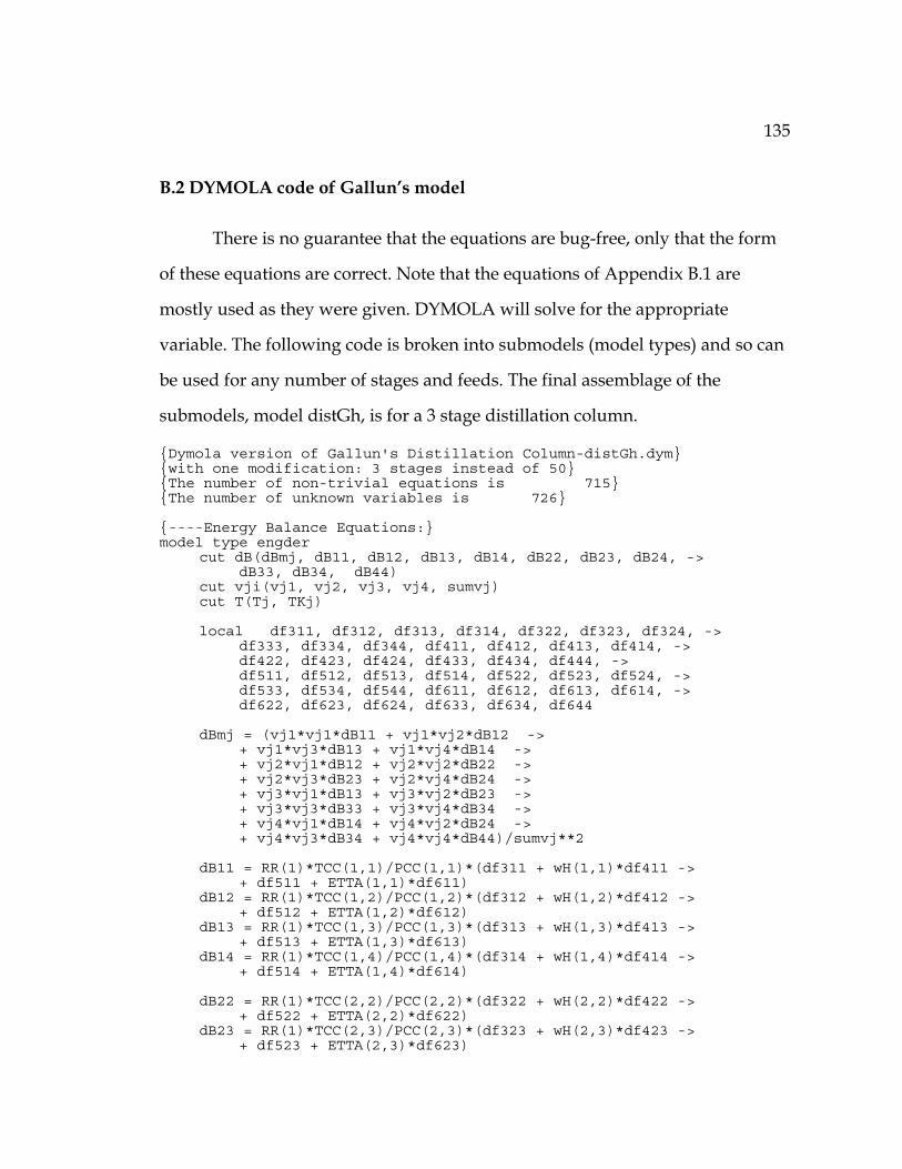
135

B.2 DYMOLA code of Gallun’s model

There is no guarantee that the equations are bug-free, only that the form

of these equations are correct. Note that the equations of Appendix B.1 are

mostly used as they were given. DYMOLA will solve for the appropriate

variable. The following code is broken into submodels (model types) and so can

be used for any number of stages and feeds. The final assemblage of the

submodels, model distGh, is for a 3 stage distillation column.

Dymola version of Gallun's Distillation Column-distGh.dym with one modification: 3 stages instead of 50 The number of non-trivial equations is 715 The number of unknown variables is 726 ----Energy Balance Equations: model type engder cut dB(dBmj, dB11, dB12, dB13, dB14, dB22, dB23, dB24, -> dB33, dB34, dB44) cut vji(vj1, vj2, vj3, vj4, sumvj) cut T(Tj, TKj) local df311, df312, df313, df314, df322, df323, df324, -> df333, df334, df344, df411, df412, df413, df414, -> df422, df423, df424, df433, df434, df444, -> df511, df512, df513, df514, df522, df523, df524, -> df533, df534, df544, df611, df612, df613, df614, -> df622, df623, df624, df633, df634, df644 dBmj = (vj1*vj1*dB11 + vj1*vj2*dB12 -> + vj1*vj3*dB13 + vj1*vj4*dB14 -> + vj2*vj1*dB12 + vj2*vj2*dB22 -> + vj2*vj3*dB23 + vj2*vj4*dB24 -> + vj3*vj1*dB13 + vj3*vj2*dB23 -> + vj3*vj3*dB33 + vj3*vj4*dB34 -> + vj4*vj1*dB14 + vj4*vj2*dB24 -> + vj4*vj3*dB34 + vj4*vj4*dB44)/sumvj**2 dB11 = RR(1)*TCC(1,1)/PCC(1,1)*(df311 + wH(1,1)*df411 -> + df511 + ETTA(1,1)*df611) dB12 = RR(1)*TCC(1,2)/PCC(1,2)*(df312 + wH(1,2)*df412 -> + df512 + ETTA(1,2)*df612) dB13 = RR(1)*TCC(1,3)/PCC(1,3)*(df313 + wH(1,3)*df413 -> + df513 + ETTA(1,3)*df613) dB14 = RR(1)*TCC(1,4)/PCC(1,4)*(df314 + wH(1,4)*df414 -> + df514 + ETTA(1,4)*df614) dB22 = RR(1)*TCC(2,2)/PCC(2,2)*(df322 + wH(2,2)*df422 -> + df522 + ETTA(2,2)*df622) dB23 = RR(1)*TCC(2,3)/PCC(2,3)*(df323 + wH(2,3)*df423 -> + df523 + ETTA(2,3)*df623)

136

dB24 = RR(1)*TCC(2,4)/PCC(2,4)*(df324 + wH(2,4)*df424 -> + df524 + ETTA(2,4)*df624) dB33 = RR(1)*TCC(3,3)/PCC(3,3)*(df333 + wH(3,3)*df433 -> + df533 + ETTA(3,3)*df633) dB34 = RR(1)*TCC(3,4)/PCC(3,4)*(df334 + wH(3,4)*df434 -> + df534 + ETTA(3,4)*df634) dB44 = RR(1)*TCC(4,4)/PCC(4,4)*(df344 + wH(4,4)*df444 -> + df544 + ETTA(4,4)*df644) df311 = -0.330*TCC(1,1)/TKj**2 + 0.1385*TCC(1,1)**2/TKj**3 -> + 0.0121*TCC(1,1)**3/TKj**4 df312 = -0.330*TCC(1,2)/TKj**2 + 0.1385*TCC(1,2)**2/TKj**3 -> + 0.0121*TCC(1,2)**3/TKj**4 df313 = -0.330*TCC(1,1)/TKj**2 + 0.1385*TCC(1,3)**2/TKj**3 -> + 0.0121*TCC(1,3)**3/TKj**4 df314 = -0.330*TCC(1,4)/TKj**2 + 0.1385*TCC(1,4)**2/TKj**3 -> + 0.0121*TCC(1,4)**3/TKj**4 df322 = -0.330*TCC(2,2)/TKj**2 + 0.1385*TCC(2,2)**2/TKj**3 -> + 0.0121*TCC(2,2)**3/TKj**4 df323 = -0.330*TCC(2,3)/TKj**2 + 0.1385*TCC(2,3)**2/TKj**3 -> + 0.0121*TCC(2,3)**3/TKj**4 df324 = -0.330*TCC(2,4)/TKj**2 + 0.1385*TCC(2,4)**2/TKj**3 -> + 0.0121*TCC(2,4)**3/TKj**4 df333 = -0.330*TCC(3,3)/TKj**2 + 0.1385*TCC(3,3)**2/TKj**3 -> + 0.0121*TCC(3,3)**3/TKj**4 df334 = -0.330*TCC(3,4)/TKj**2 + 0.1385*TCC(3,4)**2/TKj**3 -> + 0.0121*TCC(3,4)**3/TKj**4 df344 = -0.330*TCC(4,4)/TKj**2 + 0.1385*TCC(4,4)**2/TKj**3 -> + 0.0121*TCC(4,4)**3/TKj**4 df411 = - 0.4600*TCC(1,1)/TKj**2 -> + 0.5000*TCC(1,1)/TKj**3 -> + 0.0970*TCC(1,1)**3/TKj**4 -> + 0.0073*TCC(1,1)**8/TKj**9 df412 = - 0.4600*TCC(1,2)/TKj**2 -> + 0.5000*TCC(1,2)/TKj**3 -> + 0.0970*TCC(1,2)**3/TKj**4 -> + 0.0073*TCC(1,2)**8/TKj**9 df413 = - 0.4600*TCC(1,3)/TKj**2 -> + 0.5000*TCC(1,3)/TKj**3 -> + 0.0970*TCC(1,3)**3/TKj**4 -> + 0.0073*TCC(1,3)**8/TKj**9 df414 = - 0.4600*TCC(1,4)/TKj**2 -> + 0.5000*TCC(1,4)/TKj**3 -> + 0.0970*TCC(1,4)**3/TKj**4 -> + 0.0073*TCC(1,4)**8/TKj**9 df422 = - 0.4600*TCC(2,2)/TKj**2 -> + 0.5000*TCC(2,2)/TKj**3 -> + 0.0970*TCC(2,2)**3/TKj**4 -> + 0.0073*TCC(2,2)**8/TKj**9 df423 = - 0.4600*TCC(2,3)/TKj**2 -> + 0.5000*TCC(2,3)/TKj**3 -> + 0.0970*TCC(2,3)**3/TKj**4 -> + 0.0073*TCC(2,3)**8/TKj**9 df424 = - 0.4600*TCC(2,4)/TKj**2 -> + 0.5000*TCC(2,4)/TKj**3 -> + 0.0970*TCC(2,4)**3/TKj**4 ->

137

+ 0.0073*TCC(2,4)**8/TKj**9 df433 = - 0.4600*TCC(3,3)/TKj**2 -> + 0.5000*TCC(3,3)/TKj**3 -> + 0.0970*TCC(3,3)**3/TKj**4 -> + 0.0073*TCC(3,3)**8/TKj**9 df434 = - 0.4600*TCC(3,4)/TKj**2 -> + 0.5000*TCC(3,4)/TKj**3 -> + 0.0970*TCC(3,4)**3/TKj**4 -> + 0.0073*TCC(3,4)**8/TKj**9 df444 = - 0.4600*TCC(4,4)/TKj**2 -> + 0.5000*TCC(4,4)/TKj**3 -> + 0.0970*TCC(4,4)**3/TKj**4 -> + 0.0073*TCC(4,4)**8/TKj**9 df511 = (5.769770 - 6.181427*MUR(1,1) -> + 2.283270*MUR(1,1)**2 -> - 0.2649074*MUR(1,1)**3) *TCC(1,1)/TKj**2 df512 = (5.769770 - 6.181427*MUR(1,2) -> + 2.283270*MUR(1,2)**2 -> - 0.2649074*MUR(1,2)**3) *TCC(1,2)/TKj**2 df513 = (5.769770 - 6.181427*MUR(1,3) -> + 2.283270*MUR(1,3)**2 -> - 0.2649074*MUR(1,3)**3) *TCC(1,3)/TKj**2 df514 = (5.769770 - 6.181427*MUR(1,4) -> + 2.283270*MUR(1,4)**2 -> - 0.2649074*MUR(1,4)**3) *TCC(1,4)/TKj**2 df522 = (5.769770 - 6.181427*MUR(2,2) -> + 2.283270*MUR(2,2)**2 -> - 0.2649074*MUR(2,2)**3) *TCC(2,2)/TKj**2 df523 = (5.769770 - 6.181427*MUR(2,3) -> + 2.283270*MUR(2,3)**2 -> - 0.2649074*MUR(2,3)**3) *TCC(2,3)/TKj**2 df524 = (5.769770 - 6.181427*MUR(2,4) -> + 2.283270*MUR(2,4)**2 -> - 0.2649074*MUR(2,4)**3) *TCC(2,4)/TKj**2 df533 = (5.769770 - 6.181427*MUR(3,3) -> + 2.283270*MUR(3,3)**2 -> - 0.2649074*MUR(3,3)**3) *TCC(3,3)/TKj**2 df534 = (5.769770 - 6.181427*MUR(3,4) -> + 2.283270*MUR(3,4)**2 -> - 0.2649074*MUR(3,4)**3) *TCC(3,4)/TKj**2 df544 = (5.769770 - 6.181427*MUR(4,4) -> + 2.283270*MUR(4,4)**2 -> - 0.2649074*MUR(4,4)**3) *TCC(4,4)/TKj**2 df611 = 101.49*EXP(-6.6*TKj/TCC(1,1)) df612 = 101.49*EXP(-6.6*TKj/TCC(1,2)) df613 = 101.49*EXP(-6.6*TKj/TCC(1,3)) df614 = 101.49*EXP(-6.6*TKj/TCC(1,4)) df622 = 101.49*EXP(-6.6*TKj/TCC(2,2)) df623 = 101.49*EXP(-6.6*TKj/TCC(2,3)) df624 = 101.49*EXP(-6.6*TKj/TCC(2,4)) df633 = 101.49*EXP(-6.6*TKj/TCC(3,3)) df634 = 101.49*EXP(-6.6*TKj/TCC(3,4))

138

df644 = 101.49*EXP(-6.6*TKj/TCC(4,4)) end model type engb1 terminal R, QC, Ej, Pj, Lj cut eql1(ZZj, Bmj) cut uji(uj1, uj2, uj3, uj4, HLDPj) cut HVjpi(HVjp1, HVjp2, HVjp3, HVjp4) cut vjpi(vjp1, vjp2, vjp3, vjp4, sumvjp) cut T(Tj, TKj) local hLj1, hLj2, hLj3, hLj4 terminal Hfj 0 = Hfj + vjp1*HVjp1 + vjp2*HVjp2 + vjp3*HVjp3+vjp4*HVjp4 - (1 + -> R)*Lj*Ej/(R * HLDPj) - QC - der(Ej) 0 = uj1*hLj1 + uj2*hLj2 + uj3*hLj3 + uj4*hLj4 - Ej hLj1 = hLCO(1,1) + hLCO(2,1)*Tj + hLCO(3,1)*Tj**2 hLj2 = hLCO(1,2) + hLCO(2,2)*Tj + hLCO(3,2)*Tj**2 hLj3 = hLCO(1,3) + hLCO(2,3)*Tj + hLCO(3,3)*Tj**2 hLj4 = hLCO(1,4) + hLCO(2,4)*Tj + hLCO(3,4)*Tj**2 end model type engbj submodel engder terminal Ej, Pj, Lj, Ljm, Ejm cut eql1(ZZj, Bmj) cut uji(uj1, uj2, uj3, uj4, HLDPj) cut ujmi(ujm1, ujm2, ujm3, ujm4, HLDPjm) cut HVji(HVj1, HVj2, HVj3, HVj4) cut HVjpi(HVjp1, HVjp2, HVjp3, HVjp4) cut vji(vj1, vj2, vj3, vj4, sumvj) cut vjpi(vjp1, vjp2, vjp3, vjp4, sumvjp) cut T(Tj, TKj) cut dB(dBmj, dB11, dB12, dB13, dB14, dB22, dB23, dB24, -> dB33, dB34, dB44) local hLj1, hLj2, hLj3, hLj4, OMEGAj, H0j1, H0j2, H0j3, H0j4 terminal Hfj connect engder:dB at dB connect engder:T at T connect engder:vji at vji 0 = Hfj + Ljm*Ejm/HLDPjm - Lj*Ej/HLDPj + vjp1*HVjp1 - vj1*HVj1 + -> vjp2*HVjp2 - vj2*HVj2 + vjp3*HVjp3 - vj3*HVj3 + vjp4*HVjp4 - -> vj4*HVj4 - der(Ej) 0 = uj1*hLj1 + uj2*hLj2 + uj3*hLj3 + uj4*hLj4 - Ej

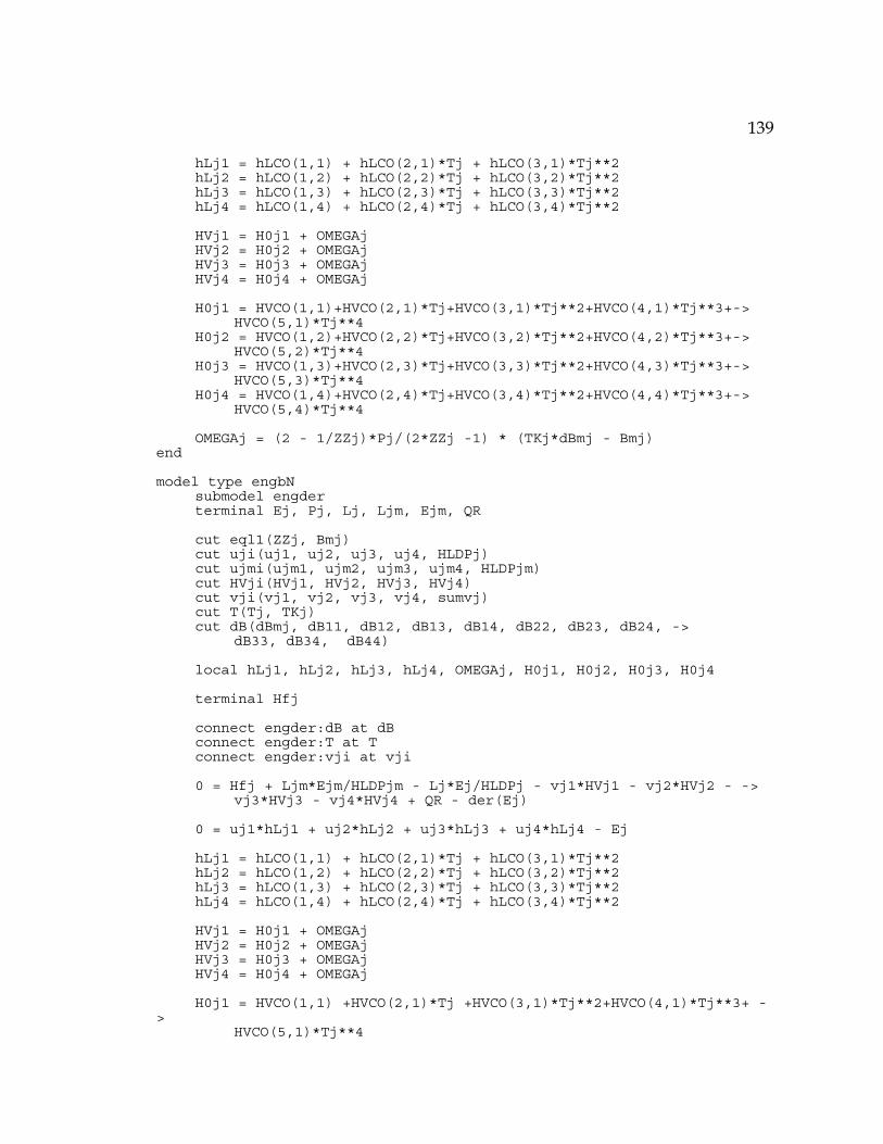
139

hLj1 = hLCO(1,1) + hLCO(2,1)*Tj + hLCO(3,1)*Tj**2 hLj2 = hLCO(1,2) + hLCO(2,2)*Tj + hLCO(3,2)*Tj**2 hLj3 = hLCO(1,3) + hLCO(2,3)*Tj + hLCO(3,3)*Tj**2 hLj4 = hLCO(1,4) + hLCO(2,4)*Tj + hLCO(3,4)*Tj**2 HVj1 = H0j1 + OMEGAj HVj2 = H0j2 + OMEGAj HVj3 = H0j3 + OMEGAj HVj4 = H0j4 + OMEGAj H0j1 = HVCO(1,1)+HVCO(2,1)*Tj+HVCO(3,1)*Tj**2+HVCO(4,1)*Tj**3+-> HVCO(5,1)*Tj**4 H0j2 = HVCO(1,2)+HVCO(2,2)*Tj+HVCO(3,2)*Tj**2+HVCO(4,2)*Tj**3+-> HVCO(5,2)*Tj**4 H0j3 = HVCO(1,3)+HVCO(2,3)*Tj+HVCO(3,3)*Tj**2+HVCO(4,3)*Tj**3+-> HVCO(5,3)*Tj**4 H0j4 = HVCO(1,4)+HVCO(2,4)*Tj+HVCO(3,4)*Tj**2+HVCO(4,4)*Tj**3+-> HVCO(5,4)*Tj**4 OMEGAj = (2 - 1/ZZj)*Pj/(2*ZZj -1) * (TKj*dBmj - Bmj) end model type engbN submodel engder terminal Ej, Pj, Lj, Ljm, Ejm, QR cut eql1(ZZj, Bmj) cut uji(uj1, uj2, uj3, uj4, HLDPj) cut ujmi(ujm1, ujm2, ujm3, ujm4, HLDPjm) cut HVji(HVj1, HVj2, HVj3, HVj4) cut vji(vj1, vj2, vj3, vj4, sumvj) cut T(Tj, TKj) cut dB(dBmj, dB11, dB12, dB13, dB14, dB22, dB23, dB24, -> dB33, dB34, dB44) local hLj1, hLj2, hLj3, hLj4, OMEGAj, H0j1, H0j2, H0j3, H0j4 terminal Hfj connect engder:dB at dB connect engder:T at T connect engder:vji at vji 0 = Hfj + Ljm*Ejm/HLDPjm - Lj*Ej/HLDPj - vj1*HVj1 - vj2*HVj2 - -> vj3*HVj3 - vj4*HVj4 + QR - der(Ej) 0 = uj1*hLj1 + uj2*hLj2 + uj3*hLj3 + uj4*hLj4 - Ej hLj1 = hLCO(1,1) + hLCO(2,1)*Tj + hLCO(3,1)*Tj**2 hLj2 = hLCO(1,2) + hLCO(2,2)*Tj + hLCO(3,2)*Tj**2 hLj3 = hLCO(1,3) + hLCO(2,3)*Tj + hLCO(3,3)*Tj**2 hLj4 = hLCO(1,4) + hLCO(2,4)*Tj + hLCO(3,4)*Tj**2 HVj1 = H0j1 + OMEGAj HVj2 = H0j2 + OMEGAj HVj3 = H0j3 + OMEGAj HVj4 = H0j4 + OMEGAj H0j1 = HVCO(1,1) +HVCO(2,1)*Tj +HVCO(3,1)*Tj**2+HVCO(4,1)*Tj**3+ -> HVCO(5,1)*Tj**4

140

H0j2 = HVCO(1,2) +HVCO(2,2)*Tj+HVCO(3,2)*Tj**2+HVCO(4,2)*Tj**3 + -> HVCO(5,2)*Tj**4 H0j3 = HVCO(1,3) +HVCO(2,3)*Tj+HVCO(3,3)*Tj**2+HVCO(4,3)*Tj**3 + -> HVCO(5,3)*Tj**4 H0j4 = HVCO(1,4) + HVCO(2,4)*Tj+HVCO(3,4)*Tj**2+HVCO(4,4)*Tj**3+ -> HVCO(5,4)*Tj**4 OMEGAj = (2 - 1/ZZj)*Pj/(2*ZZj -1) * (TKj*dBmj - Bmj) end ----Material Balance Equations: model type matb1 cut uji(uj1, uj2, uj3, uj4, HLDP1) cut vjpi(vjp1, vjp2, vjp3, vjp4, sumvjp) terminal R, Lj terminal fj1, fj2, fj3, fj4 0 = fj1 - (1 + R)*Lj*uj1/(R * HLDP1) + vjp1 - der(uj1) 0 = fj2 - (1 + R)*Lj*uj2/(R * HLDP1) + vjp2 - der(uj2) 0 = fj3 - (1 + R)*Lj*uj3/(R * HLDP1) + vjp3 - der(uj3) 0 = fj4 - (1 + R)*Lj*uj4/(R * HLDP1) + vjp4 - der(uj4) HLDP1 = uj1 + uj2 + uj3 + uj4 end model type matbj cut uji(uj1, uj2, uj3, uj4, HLDPj) cut ujmi(ujm1, ujm2, ujm3, ujm4, HLDPjm) cut vji(vj1, vj2, vj3, vj4, sumvj) cut vjpi(vjp1, vjp2, vjp3, vjp4, sumvjp) terminal Lj, Ljm terminal fj1, fj2, fj3, fj4 0 = fj1 + Ljm*ujm1/HLDPjm - Lj*uj1/HLDPj - vj1 + vjp1 - der(uj1) 0 = fj2 + Ljm*ujm2/HLDPjm - Lj*uj2/HLDPj - vj2 + vjp2 - der(uj2) 0 = fj3 + Ljm*ujm3/HLDPjm - Lj*uj3/HLDPj - vj3 + vjp3 - der(uj3) 0 = fj4 + Ljm*ujm4/HLDPjm - Lj*uj4/HLDPj - vj4 + vjp4 - der(uj4) HLDPj = uj1 + uj2 + uj3 + uj4 end model type matbN cut uji(uj1, uj2, uj3, uj4, HLDPj) cut ujmi(ujm1, ujm2, ujm3, ujm4, HLDPjm) cut vji(vj1, vj2, vj3, vj4, sumvj) terminal Lj, Ljm terminal fj1, fj2, fj3, fj4 0 = fj1 + Ljm*ujm1/HLDPjm - Lj*uj1/HLDPj - vj1 - der(uj1) 0 = fj2 + Ljm*ujm2/HLDPjm - Lj*uj2/HLDPj - vj2 - der(uj2) 0 = fj3 + Ljm*ujm3/HLDPjm - Lj*uj3/HLDPj - vj3 - der(uj3) 0 = fj4 + Ljm*ujm4/HLDPjm - Lj*uj4/HLDPj - vj4 - der(uj4) HLDPj = uj1 + uj2 + uj3 + uj4 end ----Equilibrium Equations: model type eqlcom

141

cut eqlc(LMBjik, ALPHji, ALPHjk, Bjik) cut T(Tj, TKj) local TRRjik, f3jik, f4jik, f5jik, f6jik parameter i, k constant RR1 = 1.314, RR2=62361.0, RR3=555.0 RR4=1.987 LMBjik = ALPHjk/ALPHji * EXP(WLMB(i,k)/(RR4*Tj)) TRRjik = TKj/TCC(i,k) PCC(i,k)*Bjik/(RR4*TCC(i,k)) = f3jik + wH(i,k)*f4jik + f5jik + -> ETTA(i,k)*f6jik f3jik = 0.1445 - 0.330/TRRjik - 0.1385/(TRRjik**2) - -> 0.0121/(TRRjik**3) f4jik = 0.073 + 0.46/TRRjik - 0.5/(TRRjik**2) -0.097/(TRRjik**3) -> - 0.0073/(TRRjik**8) f5jik = -5.237220 + 5.665807*MUR(i,k) - 2.133816*MUR(i,k)**2 + -> 0.2525373*MUR(i,k)**3 + (5.769770 - 6.181427*MUR(i,k) + -> 2.283270*MUR(i,k)**2 - 0.2649074*MUR(i,k)**3)/TRRjik f6jik = EXP(4.62 - 6.6*TRRjik) end model type eqlbm1 submodel (eqlcom) eqlc11(i = 1, k = 1), eqlc12(i = 1, k = 2), -> eqlc13(i=1, k=3), eqlc14(i=1, k=4), eqlc21(i=2, k=1), -> eqlc22(i=2, k=2), eqlc23(i=2, k=3), eqlc24(i=2, k=4), -> eqlc31(i=3, k=1), eqlc32(i=3, k=2), eqlc33(i=3, k=3), -> eqlc34(i=3, k=4), eqlc41(i=4, k=1), eqlc42(i=4, k=2), -> eqlc43(i = 4, k = 3), eqlc44(i = 4, k = 4) cut uji(uj1, uj2, uj3, uj4, HLDPj) cut Yji(Y11, Y12, Y13, Y14, sumvj) cut T(Tj,TKj) cut eql1(ZZj, Bmj) cut eql2(Kj1, Kj2, Kj3 ,Kj4) cut eql11(LMBj11, ALPHj1, ALPHj1, Bj11) cut eql12(LMBj12, ALPHj1, ALPHj2, Bj12) cut eql13(LMBj13, ALPHj1, ALPHj3, Bj13) cut eql14(LMBj14, ALPHj1, ALPHj4, Bj14) cut eql21(LMBj21, ALPHj2, ALPHj1, Bj21) cut eql22(LMBj22, ALPHj2, ALPHj2, Bj22) cut eql23(LMBj23, ALPHj2, ALPHj3, Bj23) cut eql24(LMBj24, ALPHj2, ALPHj4, Bj24) cut eql31(LMBj31, ALPHj3, ALPHj1, Bj31) cut eql32(LMBj32, ALPHj3, ALPHj2, Bj32) cut eql33(LMBj33, ALPHj3, ALPHj3, Bj33) cut eql34(LMBj34, ALPHj3, ALPHj4, Bj34) cut eql41(LMBj41, ALPHj4, ALPHj1, Bj41) cut eql42(LMBj42, ALPHj4, ALPHj2, Bj42) cut eql43(LMBj43, ALPHj4, ALPHj3, Bj43) cut eql44(LMBj44, ALPHj4, ALPHj4, Bj44) terminal Pj local Vmj, PHIVj1, PHIVj2, PHIVj3, PHIVj4, GAMj1, GAMj2, GAMj3, -> GAMj4, PHILj1, PSj1, PHISj1, f1j1, f2j1, TRj1, -> PHILj2, PSj2, PHISj2, f1j2, f2j2, TRj2, ->

142

PHILj3, PSj3, PHISj3, f1j3, f2j3, TRj3, -> PHILj4, PSj4, PHISj4, f1j4, f2j4, TRj4 parameter RR1 = 1.314, RR2=62361.0, RR3=555.0, RR4=1.987 connect eqlc11:eqlc at eql11 connect eqlc12:eqlc at eql12 connect eqlc13:eqlc at eql13 connect eqlc14:eqlc at eql14 connect eqlc21:eqlc at eql21 connect eqlc22:eqlc at eql22 connect eqlc23:eqlc at eql23 connect eqlc24:eqlc at eql24 connect eqlc31:eqlc at eql31 connect eqlc32:eqlc at eql32 connect eqlc33:eqlc at eql33 connect eqlc34:eqlc at eql34 connect eqlc41:eqlc at eql41 connect eqlc42:eqlc at eql42 connect eqlc43:eqlc at eql43 connect eqlc44:eqlc at eql44 connect eqlc11:T at T connect eqlc12:T at T connect eqlc13:T at T connect eqlc14:T at T connect eqlc21:T at T connect eqlc22:T at T connect eqlc23:T at T connect eqlc24:T at T connect eqlc31:T at T connect eqlc32:T at T connect eqlc33:T at T connect eqlc34:T at T connect eqlc41:T at T connect eqlc42:T at T connect eqlc43:T at T connect eqlc44:T at T 0 = Y11*PHIVj1 - uj1*GAMj1*Kj1*PHILj1/HLDPj 0 = Y12*PHIVj2 - uj2*GAMj2*Kj2*PHILj2/HLDPj 0 = Y13*PHIVj3 - uj3*GAMj3*Kj3*PHILj3/HLDPj 0 = Y14*PHIVj4 - uj4*GAMj4*Kj4*PHILj4/HLDPj Y11 + Y12 + Y13 + Y14 = 1 sumvj = Y11 + Y12 + Y13 + Y14 Kj1 = PSj1/Pj GAMj1 = EXP(1 - uj1*LMBj11/(uj1*LMBj11 + uj1*LMBj12 + uj1*LMBj13 -> + uj1*LMBj14) + uj2*LMBj21/(uj2*LMBj21 + uj2*LMBj22 + -> uj2*LMBj23 + uj2*LMBj24) + uj3*LMBj31/(uj3*LMBj31 + -> uj3*LMBj32 + uj3*LMBj33 + uj3*LMBj34) + -> uj4*LMBj41/(uj4*LMBj41 + uj4*LMBj42 + uj4*LMBj43 + -> uj4*LMBj44)) * HLDPj/(uj1*LMBj11 + uj2*LMBj21 +uj3*LMBj31 + -> uj4*LMBj41) ALPHj1 = MV(1,1) + MV(2,1)*Tj + MV(3,1)*Tj**2 PHISj1 = EXP(f1j1 + f2j1 + WW(1)) TRj1 = Tj/TC(1) f1j1 = -3.5021358 + TRj1*( 5.6085595 + TRj1*(-3.076574 + -> TRj1*0.57335015))

143

f2j1 = -3.7690418 + TRj1*( 4.3538729 + TRj1*( 0.3166137 + TRj1*( -> 0.12666184 + TRj1*(-1.1662283 + TRj1*(-0.10665730 + TRj1*( -> 0.12147436 + TRj1*( 0.18927037 + TRj1*(0.14936906 + -> TRj1*(0.024364816 + TRj1*(-0.068603516 + TRj1*(-0.015172164 -> + TRj1*0.012089114))))))))))) PHILj1 = PHISj1*EXP(-ALPHj1*PSj1/(RR2*TKj)) PHIVj1 = exp(2*(Y11*Bj11 + Y12*Bj12 + Y13*Bj13 + -> Y14*Bj14)/(Vmj*(Y11 + Y12 + Y13 + Y14)) ) - ZZj PSj1 = ALOG10(ANT(1,1) - (ANT(2,1)/(ANT(3,1) + (TKj - 273.15)))) -------------- Kj2 = PSj2/Pj GAMj2 = EXP(1 - uj1*LMBj12/(uj1*LMBj11 + uj1*LMBj12 +uj1*LMBj13 -> + uj1*LMBj14) + uj2*LMBj22/(uj2*LMBj21 + uj2*LMBj22 + -> uj2*LMBj23 + uj2*LMBj24) + uj3*LMBj32/(uj3*LMBj31 + -> uj3*LMBj32 + uj3*LMBj33 + uj3*LMBj34) + -> uj4*LMBj42/(uj4*LMBj41 + uj4*LMBj42 + uj4*LMBj43 + -> uj4*LMBj44)) * HLDPj/(uj1*LMBj12 + uj2*LMBj22 +uj3*LMBj32 + -> uj4*LMBj42) ALPHj2 = MV(1,2) + MV(2,2)*Tj + MV(3,2)*Tj**2 PHISj2 = EXP(f1j2 + f2j2 + WW(2)) TRj2 = TKj/TC(2) f1j2 = -3.5021358 + TRj2*( 5.6085595 + TRj2*(-3.076574 + -> TRj2*0.57335015)) f2j2 = -3.7690418 + TRj2*( 4.3538729 + TRj2*( 0.3166137 + TRj2*( -> 0.12666184 + TRj2*(-1.1662283 + TRj2*(-0.10665730 + TRj2*( -> 0.12147436 + TRj2*( 0.18927037 + TRj2*(0.14936906 + -> TRj2*(0.024364816 + TRj2*(-0.068603516 + TRj2*(-0.015172164 -> + TRj2*0.012089114))))))))))) PHILj2 = PHISj2*EXP(-ALPHj2*PSj2/(RR2*TKj)) PHIVj2 = exp(2*(Y11*Bj21 + Y12*Bj22 + Y13*Bj23 + -> Y14*Bj24)/(Vmj*(Y11 + Y12 + Y13 + Y14)) ) - ZZj PSj2 = ALOG10(ANT(1,2) - (ANT(2,2)/(ANT(3,2) + (TKj - 273.15)))) -------------- Kj3 = PSj3/Pj GAMj3 = EXP(1 - uj1*LMBj13/(uj1*LMBj11 + uj1*LMBj12 +uj1*LMBj13 -> + uj1*LMBj14) + uj2*LMBj23/(uj2*LMBj21 + uj2*LMBj22 + -> uj2*LMBj23 + uj2*LMBj24) + uj3*LMBj33/(uj3*LMBj31 + -> uj3*LMBj32 + uj3*LMBj33 + uj3*LMBj34) + -> uj4*LMBj43/(uj4*LMBj41 + uj4*LMBj42 + uj4*LMBj43 + -> uj4*LMBj44)) * HLDPj/(uj1*LMBj13 + uj2*LMBj23 +uj3*LMBj33 + -> uj4*LMBj43) ALPHj3 = MV(1,3) + MV(2,3)*Tj + MV(3,3)*Tj**2 PHISj3 = EXP(f1j3 + f2j3 + WW(3)) TRj3 = TKj/TC(3) f1j3 = -3.5021358 + TRj3*( 5.6085595 + TRj3*(-3.076574 + -> TRj3*0.57335015)) f2j3 = -3.7690418 + TRj3*( 4.3538729 + TRj3*( 0.3166137 + TRj3*( -> 0.12666184 + TRj3*(-1.1662283 + TRj3*(-0.10665730 + TRj3*( -> 0.12147436 + TRj3*( 0.18927037 + TRj3*(0.14936906 + -> TRj3*(0.024364816 + TRj3*(-0.068603516 + TRj3*(-0.015172164 -> + TRj3*0.012089114))))))))))) PHILj3 = PHISj3*EXP(-ALPHj3*PSj3/(RR2*TKj)) PHIVj3 = exp(2*(Y11*Bj31 + Y12*Bj32 + Y13*Bj33 + -> Y14*Bj34)/(Vmj*(Y11 + Y12 + Y13 + Y14)) ) - ZZj

144

PSj3 = ALOG10(ANT(1,3) - (ANT(2,3)/(ANT(3,3) + (TKj - 273.15)))) ----------- Kj4 = PSj4/Pj GAMj4 = EXP(1 - uj1*LMBj14/(uj1*LMBj11 + uj1*LMBj12 +uj1*LMBj13 -> + uj1*LMBj14) + uj2*LMBj24/(uj2*LMBj21 + uj2*LMBj22 + -> uj2*LMBj23 + uj2*LMBj24) + uj3*LMBj34/(uj3*LMBj31 + -> uj3*LMBj32 + uj3*LMBj33 + uj3*LMBj34) + -> uj4*LMBj44/(uj4*LMBj41 + uj4*LMBj42 + uj4*LMBj43 + -> uj4*LMBj44)) * HLDPj/(uj1*LMBj14 + uj2*LMBj24 +uj3*LMBj34 + -> uj4*LMBj44) ALPHj4 = MV(1,4) + MV(2,4)*Tj + MV(3,4)*Tj**2 PHISj4 = EXP(f1j4 + f2j4 + WW(4)) TRj4 = TKj/TC(4) f1j4 = -3.5021358 + TRj4*( 5.6085595 + TRj4*(-3.076574 + -> TRj4*0.57335015)) f2j4 = -3.7690418 + TRj4*( 4.3538729 + TRj4*( 0.3166137 + TRj4*( -> 0.12666184 + TRj4*(-1.1662283 + TRj4*(-0.10665730 + TRj4*( -> 0.12147436 + TRj4*( 0.18927037 + TRj4*(0.14936906 + -> TRj4*(0.024364816 + TRj4*(-0.068603516 + TRj4*(-0.015172164 -> + TRj4*0.012089114))))))))))) PHILj4 = PHISj4*EXP(-ALPHj4*PSj4/(RR2*TKj)) PHIVj4 = exp(2*(Y11*Bj41 + Y12*Bj42 + Y13*Bj43 + -> Y14*Bj44)/(Vmj*(Y11 + Y12 + Y13 + Y14)) ) - ZZj PSj4 = ALOG10(ANT(1,4) - (ANT(2,4)/(ANT(3,4) + (TKj - 273.15)))) --------- Bmj = ( Y11*(Y11*Bj11 + Y12*Bj12 + Y13*Bj13 + Y14*Bj14) + -> Y12*(Y11*Bj21 + Y12*Bj22 + Y13*Bj23 + Y14*Bj24) + -> Y13*(Y11*Bj31 + Y12*Bj32 + Y13*Bj33 + Y14*Bj34) + -> Y14*(Y11*Bj41 + Y12*Bj42 + Y13*Bj43 + Y14*Bj44))/(Y11 + Y12 -> + Y13 + Y14)**2 TKj = 5.0*Tj/9.0 ZZj = (1. + SQRT(1. + 4*Bmj*Pj/(RR3*TKj)))/2.0 Vmj = Bmj/(ZZj - 1) end model type eqlbm submodel (eqlcom) eqlc11(i = 1, k = 1), eqlc12(i = 1, k = 2), -> eqlc13(i=1, k=3), eqlc14(i= 1, k = 4), eqlc21(i = 2, k = 1), -> eqlc22(i=2, k=2), eqlc23(i= 2, k = 3), eqlc24(i = 2, k = 4), -> eqlc31(i=3, k=1), eqlc32(i= 3, k = 2), eqlc33(i = 3, k = 3), -> eqlc34(i=3, k=4), eqlc41(i= 4, k = 1), eqlc42(i = 4, k = 2), -> eqlc43(i = 4, k = 3), eqlc44(i = 4, k = 4) cut uji(uj1, uj2, uj3, uj4, HLDPj) cut T(Tj,TKj) cut vji(vj1, vj2, vj3, vj4, sumvj) cut eql1(ZZj, Bmj) cut eql2(Kj1, Kj2, Kj3 ,Kj4) cut eql11(LMBj11, ALPHj1, ALPHj1, Bj11) cut eql12(LMBj12, ALPHj1, ALPHj2, Bj12) cut eql13(LMBj13, ALPHj1, ALPHj3, Bj13) cut eql14(LMBj14, ALPHj1, ALPHj4, Bj14) cut eql21(LMBj21, ALPHj2, ALPHj1, Bj21) cut eql22(LMBj22, ALPHj2, ALPHj2, Bj22)

145

cut eql23(LMBj23, ALPHj2, ALPHj3, Bj23) cut eql24(LMBj24, ALPHj2, ALPHj4, Bj24) cut eql31(LMBj31, ALPHj3, ALPHj1, Bj31) cut eql32(LMBj32, ALPHj3, ALPHj2, Bj32) cut eql33(LMBj33, ALPHj3, ALPHj3, Bj33) cut eql34(LMBj34, ALPHj3, ALPHj4, Bj34) cut eql41(LMBj41, ALPHj4, ALPHj1, Bj41) cut eql42(LMBj42, ALPHj4, ALPHj2, Bj42) cut eql43(LMBj43, ALPHj4, ALPHj3, Bj43) cut eql44(LMBj44, ALPHj4, ALPHj4, Bj44) terminal Pj, Vmj local PHIVj1, PHIVj2, PHIVj3, PHIVj4, GAMj1, GAMj2, GAMj3, -> GAMj4, PHILj1, PSj1, PHISj1, f1j1, f2j1, TRj1, -> PHILj2, PSj2, PHISj2, f1j2, f2j2, TRj2, -> PHILj3, PSj3, PHISj3, f1j3, f2j3, TRj3, -> PHILj4, PSj4, PHISj4, f1j4, f2j4, TRj4 parameter RR1 = 1.314, RR2=62361.0, RR3=555.0, RR4=1.987 connect eqlc11:eqlc at eql11 connect eqlc12:eqlc at eql12 connect eqlc13:eqlc at eql13 connect eqlc14:eqlc at eql14 connect eqlc21:eqlc at eql21 connect eqlc22:eqlc at eql22 connect eqlc23:eqlc at eql23 connect eqlc24:eqlc at eql24 connect eqlc31:eqlc at eql31 connect eqlc32:eqlc at eql32 connect eqlc33:eqlc at eql33 connect eqlc34:eqlc at eql34 connect eqlc41:eqlc at eql41 connect eqlc42:eqlc at eql42 connect eqlc43:eqlc at eql43 connect eqlc44:eqlc at eql44 connect eqlc11:T at T connect eqlc12:T at T connect eqlc13:T at T connect eqlc14:T at T connect eqlc21:T at T connect eqlc22:T at T connect eqlc23:T at T connect eqlc24:T at T connect eqlc31:T at T connect eqlc32:T at T connect eqlc33:T at T connect eqlc34:T at T connect eqlc41:T at T connect eqlc42:T at T connect eqlc43:T at T connect eqlc44:T at T 0 = vj1*PHIVj1/(vj1 + vj2 + vj3 + vj4) - -> uj1*GAMj1*Kj1*PHILj1/HLDPj Kj1 = PSj1/Pj GAMj1 = EXP(1 - uj1*LMBj11/(uj1*LMBj11 + uj1*LMBj12 +uj1*LMBj13 -> + uj1*LMBj14) + uj2*LMBj21/(uj2*LMBj21 + uj2*LMBj22 + ->

146

uj2*LMBj23 + uj2*LMBj24) + uj3*LMBj31/(uj3*LMBj31 + -> uj3*LMBj32 + uj3*LMBj33 + uj3*LMBj34) + -> uj4*LMBj41/(uj4*LMBj41 + uj4*LMBj42 + uj4*LMBj43 + -> uj4*LMBj44)) * HLDPj/(uj1*LMBj11 + uj2*LMBj21 +uj3*LMBj31 + -> uj4*LMBj41) ALPHj1 = MV(1,1) + MV(2,1)*Tj + MV(3,1)*Tj**2 PHISj1 = EXP(f1j1 + f2j1 + WW(1)) TRj1 = Tj/TC(1) f1j1 = -3.5021358 + TRj1*( 5.6085595 + TRj1*(-3.076574 + -> TRj1*0.57335015)) f2j1 = -3.7690418 + TRj1*( 4.3538729 + TRj1*( 0.3166137 + TRj1*( -> 0.12666184 + TRj1*(-1.1662283 + TRj1*(-0.10665730 + TRj1*( -> 0.12147436 + TRj1*( 0.18927037 + TRj1*(0.14936906 + -> TRj1*(0.024364816 + TRj1*(-0.068603516 + TRj1*(-0.015172164 -> + TRj1*0.012089114))))))))))) PHILj1 = PHISj1*EXP(-ALPHj1*PSj1/(RR2*TKj)) PHIVj1 = exp(2*(vj1*Bj11 + vj2*Bj12 + vj3*Bj13 + -> vj4*Bj14)/(Vmj*(vj1 + vj2 + vj3 + vj4)) ) - ZZj PSj1 = ALOG10(ANT(1,1) - (ANT(2,1)/(ANT(3,1) + (TKj - 273.15)))) -------------- 0 = vj2*PHIVj2/(vj1 + vj2 + vj3 + vj4) - -> uj2*GAMj2*Kj2*PHILj2/HLDPj Kj2 = PSj2/Pj GAMj2 = EXP(1 - uj1*LMBj12/(uj1*LMBj11 + uj1*LMBj12 +uj1*LMBj13 -> + uj1*LMBj14) + uj2*LMBj22/(uj2*LMBj21 + uj2*LMBj22 + -> uj2*LMBj23 + uj2*LMBj24) + uj3*LMBj32/(uj3*LMBj31 + -> uj3*LMBj32 + uj3*LMBj33 + uj3*LMBj34) + -> uj4*LMBj42/(uj4*LMBj41 + uj4*LMBj42 + uj4*LMBj43 + -> uj4*LMBj44)) * HLDPj/(uj1*LMBj12 + uj2*LMBj22 +uj3*LMBj32 + -> uj4*LMBj42) ALPHj2 = MV(1,2) + MV(2,2)*Tj + MV(3,2)*Tj**2 PHISj2 = EXP(f1j2 + f2j2 + WW(2)) TRj2 = TKj/TC(2) f1j2 = -3.5021358 + TRj2*( 5.6085595 + TRj2*(-3.076574 + -> TRj2*0.57335015)) f2j2 = -3.7690418 + TRj2*( 4.3538729 + TRj2*( 0.3166137 + TRj2*( -> 0.12666184 + TRj2*(-1.1662283 + TRj2*(-0.10665730 + TRj2*( -> 0.12147436 + TRj2*( 0.18927037 + TRj2*(0.14936906 + -> TRj2*(0.024364816 + TRj2*(-0.068603516 + TRj2*(-0.015172164 -> + TRj2*0.012089114))))))))))) PHILj2 = PHISj2*EXP(-ALPHj2*PSj2/(RR2*TKj)) PHIVj2 = exp(2*(vj1*Bj21 + vj2*Bj22 + vj3*Bj23 + -> vj4*Bj24)/(Vmj*(vj1 + vj2 + vj3 + vj4)) ) - ZZj PSj2 = ALOG10(ANT(1,2) - (ANT(2,2)/(ANT(3,2) + (TKj - 273.15)))) -------------- 0 = vj3*PHIVj3/(vj1 + vj2 + vj3 + vj4) - -> uj3*GAMj3*Kj3*PHILj3/HLDPj Kj3 = PSj3/Pj GAMj3 = EXP(1 - uj1*LMBj13/(uj1*LMBj11 + uj1*LMBj12 +uj1*LMBj13 -> + uj1*LMBj14) + uj2*LMBj23/(uj2*LMBj21 + uj2*LMBj22 + -> uj2*LMBj23 + uj2*LMBj24) + uj3*LMBj33/(uj3*LMBj31 + -> uj3*LMBj32 + uj3*LMBj33 + uj3*LMBj34) + -> uj4*LMBj43/(uj4*LMBj41 + uj4*LMBj42 + uj4*LMBj43 + ->

147

uj4*LMBj44)) * HLDPj/(uj1*LMBj13 + uj2*LMBj23 +uj3*LMBj33 + -> uj4*LMBj43) ALPHj3 = MV(1,3) + MV(2,3)*Tj + MV(3,3)*Tj**2 PHISj3 = EXP(f1j3 + f2j3 + WW(3)) TRj3 = TKj/TC(3) f1j3 = -3.5021358 + TRj3*( 5.6085595 + TRj3*(-3.076574 + -> TRj3*0.57335015)) f2j3 = -3.7690418 + TRj3*( 4.3538729 + TRj3*( 0.3166137 + TRj3*( -> 0.12666184 + TRj3*(-1.1662283 + TRj3*(-0.10665730 + TRj3*( -> 0.12147436 + TRj3*( 0.18927037 + TRj3*(0.14936906 + -> TRj3*(0.024364816 + TRj3*(-0.068603516 + TRj3*(-0.015172164 -> + TRj3*0.012089114))))))))))) PHILj3 = PHISj3*EXP(-ALPHj3*PSj3/(RR2*TKj)) PHIVj3 = exp(2*(vj1*Bj31 + vj2*Bj32 + vj3*Bj33 + -> vj4*Bj34)/(Vmj*(vj1 + vj2 + vj3 + vj4)) ) - ZZj PSj3 = ALOG10(ANT(1,3) - (ANT(2,3)/(ANT(3,3) + (TKj - 273.15)))) ----------- 0 = vj4*PHIVj4/(vj1 + vj2 + vj3 + vj4) - -> uj4*GAMj4*Kj4*PHILj4/HLDPj Kj4 = PSj4/Pj GAMj4 = EXP(1 - uj1*LMBj14/(uj1*LMBj11 + uj1*LMBj12 +uj1*LMBj13 -> + uj1*LMBj14) + uj2*LMBj24/(uj2*LMBj21 + uj2*LMBj22 + -> uj2*LMBj23 + uj2*LMBj24) + uj3*LMBj34/(uj3*LMBj31 + -> uj3*LMBj32 + uj3*LMBj33 + uj3*LMBj34) + -> uj4*LMBj44/(uj4*LMBj41 + uj4*LMBj42 + uj4*LMBj43 + -> uj4*LMBj44)) * HLDPj/(uj1*LMBj14 + uj2*LMBj24 +uj3*LMBj34 + -> uj4*LMBj44) ALPHj4 = MV(1,4) + MV(2,4)*Tj + MV(3,4)*Tj**2 PHISj4 = EXP(f1j4 + f2j4 + WW(4)) TRj4 = TKj/TC(4) f1j4 = -3.5021358 + TRj4*( 5.6085595 + TRj4*(-3.076574 + -> TRj4*0.57335015)) f2j4 = -3.7690418 + TRj4*( 4.3538729 + TRj4*( 0.3166137 + TRj4*( -> 0.12666184 + TRj4*(-1.1662283 + TRj4*(-0.10665730 + TRj4*( -> 0.12147436 + TRj4*( 0.18927037 + TRj4*(0.14936906 + -> TRj4*(0.024364816 + TRj4*(-0.068603516 + TRj4*(-0.015172164 -> + TRj4*0.012089114))))))))))) PHILj4 = PHISj4*EXP(-ALPHj4*PSj4/(RR2*TKj)) PHIVj4 = exp(2*(vj1*Bj41 + vj2*Bj42 + vj3*Bj43 + -> vj4*Bj44)/(Vmj*(vj1 + vj2 + vj3 + vj4)) ) - ZZj PSj4 = ALOG10(ANT(1,4) - (ANT(2,4)/(ANT(3,4) + (TKj - 273.15)))) ------------ Bmj = ( vj1*(vj1*Bj11 + vj2*Bj12 + vj3*Bj13 + vj4*Bj14) + -> vj2*(vj1*Bj21 + vj2*Bj22 + vj3*Bj23 + vj4*Bj24) + -> vj3*(vj1*Bj31 + vj2*Bj32 + vj3*Bj33 + vj4*Bj34) + -> vj4*(vj1*Bj41 + vj2*Bj42 + vj3*Bj43 + vj4*Bj44))/(vj1 + vj2 -> + vj3 + vj4)**2 TKj = 5.0*Tj/9.0 sumvj = vj1 + vj2 + vj3 + vj4 ZZj = (1. + SQRT(1. + 4*Bmj*Pj/(RR3*TKj)))/2.0 Vmj = Bmj/(ZZj - 1) end

148

----Pressure Drop Equations: model type pres1 terminal P1, P2, RHMV2, RHML1, Z1 cut uji(uj1, uj2, uj3, uj4, HLDPj) cut vjpi(v21, v22, v23, v24, sumvjp) local VOLREC parameter REF1 = 0.947775644, LR=16.0, pii=3.141592653, DR=10.0 0 = P1 - P2 - sumvjp**2 * RHMV2*REF1 0 = HLDPj - RHML1*VOLREC VOLREC = LR*((pii/2.0 + ASIN(2*Z1/DR - 1)) *(DR/2.0)**2 + (Z1 - -> DR/2.0)*(Z1*DR - Z1**2)**0.5) end model type presj terminal Pj, Pjp, RHOLj, RHOLjp, RHOVj, RHOVjp,Lj,RHMVj, RHMVjp, -> Zj, HCTRj, HCTRjp, Vmj cut uji(uj1, uj2, uj3, uj4, HLDPj) cut vji(vj1, vj2, vj3, vj4, sumvj) cut vjpi(vjp1, vjp2, vjp3, vjp4, sumvjp) local HOj, FOAMj, QLj, FVAj, UVAj, UHj, HLUDj, RHMLj, HOLDj terminal CDj, AHj AN = AA ??????? parameter gc=32.17, g=32.0898, LW=130.806, HW=1.0, AN=141.372, -> AUD=0.908375, AA=141.372, AD=17.6715 RHMVj = 1/Vmj 0 = Pjp - Pj - g*760*RHOLj/(gc*14.696*1728.0) * (HOj + HCTRj) HOj = 0.186*(UHj/CDj)**2 * RHOVjp/RHOLj HCTRj = FOAMj*(0.4896*(QLj/LW)**0.67 + HW) QLj = 7.48*Lj/RHMLj UVAj = sumvj/(AN*RHMVj*60) FVAj = UVAj*SQRT(RHOVj) FOAMj = 1 - 0.372192*FVAj**0.177709 UHj = sumvjp/(AHj*RHMVjp*60) 0 = Pj - Pjp + g*760/(gc*14.696*1728) * ((12*Zj - HLUDj)*RHOLj - -> HCTRjp*RHOLjp) HLUDj = 0.000003*(QLj/AUD)**2 0 = HLDPj - HOLDj HOLDj = RHMLj*(HCTRj*AA/12.0 + Zj*AD) end model type presN terminal Z50, RHML50, q50, HCTRj, RHMVj, RHOVj, Vmj cut uji(uj1, uj2, uj3, uj4, HLDPj) cut vji(vj1, vj2, vj3, vj4, sumvj) local VOLBTW, FOAMj, UVAj, FVAj parameter AN=141.372, LW=130.806, HW=1.0, pii=3.141592653, -> DTT=15.0 RHMVj = 1/Vmj

149

0 = HLDPj - RHML50*VOLBTW VOLBTW = 100 + pii*Z50*DTT**2/4 HCTRj = FOAMj*(0.4896*(q50/LW)**0.67 + HW) UVAj = sumvj/(AN*RHMVj*60) FVAj = UVAj*SQRT(RHOVj) FOAMj = 1 - 0.372192*FVAj**0.177709 end ----Condenser and Receiver Equations: model type condsr terminal QC, L1, RHML1, R, P2, Z1, P1, q1 cut T(T1,TK1) cut Tp(T2,TK2) cut vjpi(v21, v22, v23, v24, sumvjp) cut contr1(CV1, CV2, CV3) local HEAD1, Pd1, Ps1, q2, Qcw, Tmc, Two, RHOL1 parameter ALPHA=0.2 , Apc=16022.16, Aw=13940.0,Ccw=1.0,Cmc=0.12, -> g=32.0898, gc=32.17, PD=40.0, Pw1=60, Pw3=35.0, REF2 = 9.0, -> Qcwo=8653.0, Twi=545, Umc=45000.0, Upmo=213.0, Uwmo=1250.0, -> ZC=5.0, Ucw=17160.0 0 = Qcw*Ccw*(Twi - Two)*8.34 + Uwmo/60 * Aw*(Tmc - -> Two)*(Qcw/Qcwo)**1.8 - Ucw*Ccw*der(Two) 0 = 105.8752/(v21 + v22 + v23 + v24) * (Upmo/60 * Apc*((1--> ALPHA)*T2 + ALPHA*T1 - Tmc))**3 - QC**3 0 = QC - Uwmo/60 * (Qcw/Qcwo)**1.8 * Aw*(Tmc - Two) - -> Umc*Cmc*der(Tmc) 0 = (Pw1 - Pw3 - REF2*(Qcw/Qcwo)**1.8)*CV1**2 - (Qcw/2)**2 0 = Pd1 - Ps1 - HEAD1 HEAD1 = 9.870927E1 - 9.794161E-3*(q1 + q2) - 1.95175E-6*(q1 + -> q2)**2 - 1.954559E-9*(q1 + q2)**3 0 = q1*RHML1 - L1*7.481 0 = R*q2 - q1 0 = q1**2 * RHOL1/62.4 - CV2**2 * (Pd1*RHOL1*g/(144*gc) - -> P2*14.696/760) 0 = q2**2 * RHOL1/62.4 - CV3**2 * (Pd1*RHOL1*g/(144*gc) - -> PD*14.696/760) 0 = RHOL1*(Ps1 - Z1 - ZC) - P1*14.696*144*gc/(760*g) end ----Reboiler and Tower Base Equations: model type reboil terminal QR, P50, RHOL50, Z50, RHML50, L50, Wsh, q50 cut T(T50,TK50) cut contr2(CS4, CV5) local Tsc, Tmr,Ps2, Pd2, RHsc, RHOSC, hLSC, Es, HVSC, HEAD2, Wsc parameter Apmr=3361.826, As=3844.168, Cmr=0.12, g=32.0898, -> gc=32.17, HSH=1262.8, PB=30.0, PSH=255.0, TSH=960.0, -> TSAT=862.7, Umr=11000.0, Upmr=300.0, Us=1000.0, Vr=68.83, -> ZB=10.0 0 = Us*As/60 * (Tsc - Tmr) - QR - Umr*Cmr*der(Tmr) 0 = Upmr*Apmr/60 * (Tmr - T50) - QR

150

0 = Ps2 - (P50*14.696*144*g/(760*gc*RHOL50) + Z50 + ZB) 0 = q50*RHML50 - L50*7.481 0 = (Pd2*RHOL50*g/(144*gc) - PB) * CV5**2 - q50**2*RHOL50/62.4 0 = PSH*CS4/60 - Wsh/2 * (1 + 0.00065*(TSH - TSAT)) 0 = Wsc - Wsh + Vr*der(RHsc) 0 = RHsc - RHOSC RHOSC = 1.031951E-2 + 1.427797E1*Tsc/610 +0.9414444*(Tsc/610)**2 -> + 2.048037*(Tsc/610)**3 + 5.956991*(Tsc/610)**4 0 = Wsh*HSH - Wsc*hLSC - Us*As/60 * (Tsc - Tmr) - der(Es) hLSC = -1.6029E2 + 8.06427E-2*Tsc + 7.361453E-5*Tsc**2 + -> 1.501012E-6*Tsc**3 - 9.9964334E-10*Tsc**4 0 = Vr*RHsc*HVSC - Es HVSC = 5.448738E2 + 8.039637E-1*Tsc + 1.931794E-3*Tsc**2 - -> 3.938661E-6*Tsc**3 + 1.907853E-9*Tsc**4 0 = Pd2 - Ps2 - HEAD2 HEAD2 = 9.152028E1 - 6.584299E-2*q50 + 7.533832E-5*q50**2 - -> 4.300139E-8*q50**3 end ----Control Equations model type contrl cut contr1(CV1, CV2, CV3) cut contr2(CS4, CV5) cut T(T35, TK35) terminal P1, q1, Z1, Z50, Wsh local CI1, CI2, CI3, CI4, CI5, CI6, CO1, CO2,CO3,CO4, CO5, CO6, -> I1, I2, I3, I4, I5, I6, TM, ZETA1, ZETA2, ZETA3, ZETA4, -> ZETA5 parameter TAUM=0.20 CV1 = CV1CO(2,ZETA1) + CV1CO(3,ZETA1)*( ZETA1 -> - CV1CO(1,ZETA1)) + CV1CO(4,ZETA1)*( ZETA1 -> - CV1CO(1,ZETA1))**2 -> + CV1CO(5,ZETA1)*(ZETA1 - CV1CO(1,ZETA1))**3 CV2 = CV2CO(2,ZETA2) + CV2CO(3,ZETA2)*( ZETA2 -> - CV2CO(1,ZETA2)) + CV2CO(4,ZETA2)*( ZETA2 -> - CV2CO(1,ZETA2))**2 -> + CV2CO(5,ZETA2)*(ZETA2 - CV2CO(1,ZETA2))**3 CV3 = CV3CO(2,ZETA3) + CV3CO(3,ZETA3)*( ZETA3 -> - CV3CO(1,ZETA3)) + CV3CO(4,ZETA3)*( ZETA3 -> - CV3CO(1,ZETA3))**2 -> + CV3CO(5,ZETA3)*(ZETA3 - CV3CO(1,ZETA3))**3 CS4 = CSCO(2,ZETA4) + CSCO(3,ZETA4)*(ZETA4 -> - CSCO(1,ZETA4)) + CSCO(4,ZETA4)*(ZETA4 -> - CSCO(1,ZETA4))**2 + CSCO(5,ZETA4)*(ZETA4 -> - CSCO(1,ZETA4))**3 CV5 = CV5CO(2,ZETA5) + CV5CO(3,ZETA5)*(ZETA5 -> - CV5CO(1,ZETA5)) + CV5CO(4,ZETA5)*(ZETA5 -> - CV5CO(1,ZETA5))**2 + CV5CO(5,ZETA5)*(ZETA5 -> - CV5CO(1,ZETA5))**3 0 = CI1 + 12.0 - 0.032*P1 0 = CO1 - XKC(1)*(CI1 - CISP(1) + I1/TAUI(1)) 0 = CI1 - CISP(1) - der(I1)

151

0 = -0.25 + 0.0625*CO1 - ZETA1 - TAUV(1)*der(ZETA1) 0 = CI2 - 4.0 - (q1/200)**2 0 = CO2 - XKC(2)*(CISP(2) - CI2 + I2/TAUI(2)) 0 = CISP(2) - CI2 - der(I2) 0 = -0.25 + 0.0625*CO2 - ZETA2 - TAUV(2)*der(ZETA2) 0 = CI3 - 4.0 - 1.6*Z1 0 = CO3 - XKC(3)*(CI3 - CISP(3) + I3/TAUI(3)) 0 = CI3 - CISP(3) - der(I3) 0 = -0.25 + 0.0625*CO3 - ZETA3 - TAUV(3)*der(ZETA3) 0 = CI5 + 20.0 - 4*Z50 0 = CO5 - XKC(5)*(CI5 - CISP(5) + I5/TAUI(5)) 0 = CI5 - CISP(5) - der(I5) 0 = -0.25 + 0.0625*CO5 - ZETA5 - TAUV(5)*der(ZETA5) 0 = CI4 - 4.0 - 16*(Wsh/3000)**2 0 = CO4 - XKC(4)*(CO4 - CI4 + I4/TAUI(4)) 0 = CO4 - CI4 - der(I4) 0 = -0.25 + 0.0625*CO4 - ZETA4 - TAUV(4)*der(ZETA4) 0 = T35 - TM - TAUM*der(TM) 0 = CO6 - XKC(6)*(CISP(6) - CI6 + I6/TAUI(6)) 0 = CISP(6) - CI6 - der(I6) 0 = CI6 + 236 - 0.4*TM end model type stageG submodel engbj submodel matbj submodel eqlbm submodel presj cut uji(uj1, uj2, uj3, uj4, HLDPj) cut ujmi(ujm1, ujm2, ujm3, ujm4, HLDPjm) cut T(Tj, TKj) cut HVji(HVj1, HVj2, HVj3, HVj4) cut HVjpi(HVjp1, HVjp2, HVjp3, HVjp4) cut vji(vj1, vj2, vj3, vj4, sumvj) cut vjpi(vjp1, vjp2, vjp3, vjp4, sumvjp) cut sup(Pjp, RHOLjp, RHOVjp, RHMVjp, HCTRjp) cut stup(Pj, RHOLj, RHOVj, RHMVj, HCTRj) cut stgup[sup, HVjpi, vjpi] cut stgupp[stup, HVji, vji] cut sdn(Ljm, Ejm) cut stdn(Lj, Ej) cut stgdn[sdn, ujmi] cut stgdnn[stdn, uji] parameter Hfj, fj1, fj2, fj3, fj4, CDj, AHj connect engbj:eql1 at eqlbm:eql1 connect engbj:uji at matbj:uji connect eqlbm:uji at matbj:uji connect presj:uji at matbj:uji connect matbj:uji at uji connect engbj:ujmi at ujmi connect matbj:ujmi at ujmi connect engbj:HVji at HVji connect engbj:HVjpi at HVjpi connect engbj:vji at eqlbm:vji connect matbj:vji at eqlbm:vji connect presj:vji at eqlbm:vji connect eqlbm:vji at vji connect engbj:vjpi at matbj:vjpi connect presj:vjpi at matbj:vjpi

152

connect matbj:vjpi at vjpi connect engbj:T at eqlbm:T connect engbj:T at T engbj.Hfj = Hfj matbj.fj1 = fj1 matbj.fj2 = fj2 matbj.fj3 = fj3 matbj.fj4 = fj4 presj.CDj = CDj presj.AHj = AHj engbj.Ej = Ej presj.Pj = Pj engbj.Pj = presj.Pj eqlbm.Pj = presj.Pj engbj.Lj = matbj.Lj engbj.Lj = Lj presj.Lj = Lj engbj.Ljm = matbj.Ljm engbj.Ljm = Ljm engbj.Ejm = Ejm presj.RHOLj = RHOLj presj.RHOLjp = RHOLjp presj.RHOVj = RHOVj presj.RHOVjp = RHOVjp presj.RHMVj = RHMVj presj.RHMVjp = RHMVjp presj.HCTRj = HCTRj presj.HCTRjp = HCTRjp eqlbm.Vmj = presj.Vmj end model type condG submodel engb1 submodel matb1 submodel eqlbm1 submodel pres1 submodel condsr cut T(Tj,TKj) cut Tp(Tjp,TKj) cut vji(vj1, vj2, vj3, vj4, sumvj) cut vjpi(vjp1, vjp2, vjp3, vjp4, sumvjp) cut uji(uj1, uj2, uj3, uj4, HLDPj) cut contr1(CV1, CV2, CV3) cut HVjpi(HVjp1, HVjp2, HVjp3, HVjp4) cut sup(Pjp, RHOLjp, RHOVjp, RHMVjp, HCTRjp) cut stgup[sup, HVjpi, vjpi] cut stdn(Lj, Ej) cut stgdnn[stdn, uji] terminal q1, P1, Z1 parameter Hfj=0, fj1=0, fj2=0, fj3=0, fj4=0 connect engb1:eql1 at eqlbm1:eql1 connect engb1:uji at matb1:uji connect eqlbm1:uji at matb1:uji connect pres1:uji at matb1:uji connect matb1:uji at uji connect engb1:HVjpi at HVjpi connect eqlbm1:Yji at vji connect engb1:vjpi at vjpi

153

connect matb1:vjpi at vjpi connect pres1:vjpi at vjpi connect condsr:vjpi at vjpi connect engb1:T at eqlbm1:T connect condsr:T at eqlbm1:T connect condsr:Tp at Tp connect condsr:contr1 at contr1 engb1.Hfj = Hfj matb1.fj1 = fj1 matb1.fj2 = fj2 matb1.fj3 = fj3 matb1.fj4 = fj4 engb1.R = condsr.R matb1.R = condsr.R engb1.QC = condsr.QC engb1.Ej = Ej engb1.Pj = pres1.P1 eqlbm1.Pj = pres1.P1 condsr.P1 = pres1.P1 pres1.P1 = P1 engb1.Lj = matb1.Lj condsr.L1 = matb1.Lj matb1.Lj = Lj pres1.P2 = Pjp condsr.P2 = Pjp pres1.RHMV2 = RHMVjp pres1.RHML1 = condsr.RHML1 pres1.Z1 = condsr.Z1 condsr.Z1 = Z1 condsr.q1 = q1 end model type reboG submodel engbN submodel matbN submodel eqlbm submodel presN submodel reboil cut uji(uj1, uj2, uj3, uj4, HLDPj) cut ujmi(ujm1, ujm2, ujm3, ujm4, HLDPjm) cut HVji(HVj1, HVj2, HVj3, HVj4) cut vji(vj1, vj2, vj3, vj4, sumvj) cut stup(Pj, RHOLj, RHOVj, RHMVj, HCTRj) cut stgupp[stup, HVji, vji] cut sdn(Ljm, Ejm) cut stgdn[sdn, ujmi] cut contr2(CS4, CV5) terminal Z50, Wsh parameter Hfj=0, fj1=0, fj2=0, fj3=0, fj4=0 connect engbN:eql1 at eqlbm:eql1 connect engbN:uji at uji connect eqlbm:uji at uji connect presN:uji at uji connect matbN:uji at uji connect engbN:ujmi at ujmi connect matbN:ujmi at ujmi connect engbN:HVji at HVji connect engbN:vji at eqlbm:vji

154

connect matbN:vji at eqlbm:vji connect presN:vji at vji connect eqlbm:vji at vji connect engbN:T at eqlbm:T connect reboil:T at eqlbm:T connect reboil:contr2 at contr2 engbN.Hfj = Hfj matbN.fj1 = fj1 matbN.fj2 = fj2 matbN.fj3 = fj3 matbN.fj4 = fj4 engbN.Pj = Pj reboil.P50 = Pj eqlbm.Pj = Pj engbN.Lj = matbN.Lj reboil.L50 = matbN.Lj engbN.Ljm = Ljm matbN.Ljm = Ljm engbN.Ejm = Ejm engbN.QR = reboil.QR presN.Z50 = Z50 reboil.Z50 = Z50 presN.RHML50 = reboil.RHML50 reboil.RHOL50 = RHOLj reboil.Wsh = Wsh presN.q50 = reboil.q50 presN.HCTRj = HCTRj presN.RHMVj = RHMVj presN.RHOVj = RHOVj eqlbm.Vmj = presN.Vmj end model distGh converting this model to 50 stages would mean adding 47 more stageG submodels and 94 more connections between the stages submodel (stageG) stag35(513543.3, 25.0, 0.5, -> 5.0, 197.5, 0.72, 13.0) submodel reboG(0.0, 0.0, 0.0, 0.0, 0.0) submodel condG(0.0, 0.0, 0.0, 0.0, 0.0) submodel contrl connect contrl:T at stag35:T connect condG:Tp at stag35:T connect contrl:contr2 at reboG:contr2 connect contrl:contr1 at condG:contr1 contrl.P1 = condG.P1 contrl.q1 = condG.q1 contrl.Z1 = condG.Z1 contrl.Z50 = reboG.Z50 contrl.Wsh = reboG.Wsh connect condG:stgdnn at stag35:stgdn connect stag35:stgdnn at reboG:stgdn connect reboG:stgupp at stag35:stgup connect stag35:stgupp at condG:stgup end

155

---------------------end of distGh.dym--------------------------------

156

B.3 DYMOLA assessment of Gallun’s model

The number of non-trivial equations is 715 The number of unknown variables is 726 Singular problem. Unassigned variables: stag35::engbj.derEj L1 T35 reboG::engbN.derEj L35 T50 stag35::matbj.deruj2 RHOL50 RHOL50 reboG::matbN.deruj1 L50 RHMV50 condG::condsr.Qcw rearrange reboG::reboil.derRHsc New stag35.RHOLj RHOL35 RHOL35 stag35.RHOVj RHOV35 RHOV35 condG.Tj T1 T1 condG.Z1 RHOL1 RHOL1 reboG.RHOVj RHOV50 RHOV50 reboG.Z50 New (RHOL50) RHMV35 Redundant equations: reboG::reboil HVSC = 5.448738E2 + 8.039637E-1*Tsc + 1.931794E-3* Tsc**2 - 3.938661E-6*Tsc**3 + 1.907853E-9*Tsc**4 System of 5 equations. Unknown variables: condG::condsr.T2 stag35::engbj.hLj1 stag35::engbj.hLj2 stag35::engbj.hLj3 stag35::engbj.hLj4 -stag35::engbj hLj1 = hLCO(1,1) + hLCO(2,1)*[condG::condsr.T2] + hLCO(3,1)*[condG::condsr.T2]**2 - 0 = stag35::matbj.uj1*[hLj1] + stag35::matbj.uj2* hLj2 + stag35::matbj.uj3*hLj3 + stag35::matbj.uj4*hLj4 - Ej - [hLj2] = hLCO(1,2) + hLCO(2,2)*condG::condsr.T2 + hLCO(3,2)*condG::condsr.T2**2 - [hLj3] = hLCO(1,3) + hLCO(2,3)*condG::condsr.T2 + hLCO(3,3)*condG::condsr.T2**2 - [hLj4] = hLCO(1,4) + hLCO(2,4)*condG::condsr.T2 + hLCO(3,4)*condG::condsr.T2**2 End of system of equations. System of equations is nonlinear. System of 5 equations. Unknown variables: condG::condsr.T1 condG::engb1.hLj1 condG::engb1.hLj2

157

condG::engb1.hLj3 condG::engb1.hLj4 -condG::engb1 hLj1 = hLCO(1,1) + hLCO(2,1)*[condG::condsr.T1] + hLCO(3,1)*[condG::condsr.T1]**2 - 0 = condG::matb1.uj1*[hLj1] + condG::matb1.uj2*hLj2 + condG::matb1.uj3*hLj3 + condG::matb1.uj4*hLj4 - Ej - [hLj2] = hLCO(1,2) + hLCO(2,2)*condG::condsr.T1 + hLCO(3,2)*condG::condsr.T1**2 - [hLj3] = hLCO(1,3) + hLCO(2,3)*condG::condsr.T1 + hLCO(3,3)*condG::condsr.T1**2 - [hLj4] = hLCO(1,4) + hLCO(2,4)*condG::condsr.T1 + hLCO(3,4)*condG::condsr.T1**2 End of system of equations. System of equations is nonlinear. System of 16 equations. Unknown variables: condG.P1 condG::engb1.ZZj PHIVj4 Y14 PHIVj3 Y13 PHIVj2 Y12 Y11 PHIVj1 Vmj condG::engb1.Bmj Kj1 Kj2 Kj3 Kj4 - condG::engb1.ZZj = (1 + SQRT(1 + 4*condG::engb1.Bmj*[ condG.P1]/(RR3*condG::condsr.TK1)))/2 - PHIVj4 = exp(2*(Y11*eqlc41.Bjik + Y12*eqlc42.Bjik + Y13*eqlc43.Bjik + Y14*eqlc44.Bjik)/(Vmj*(Y11 + Y12 + Y13 + Y14))) - [ condG::engb1.ZZj] - 0 = Y14*[PHIVj4] - condG::matb1.uj4*GAMj4*Kj4*PHILj4/ condG::pres1.HLDPj - PHIVj3 = exp(2*(Y11*eqlc31.Bjik + Y12*eqlc32.Bjik + Y13*eqlc33.Bjik + [Y14]*eqlc34.Bjik)/(Vmj*(Y11 + Y12 + Y13 + [Y14]) )) - condG::engb1.ZZj - 0 = Y13*[PHIVj3] - condG::matb1.uj3*GAMj3*Kj3*PHILj3/ condG::pres1.HLDPj - PHIVj2 = exp(2*(Y11*eqlc21.Bjik + Y12*eqlc22.Bjik + [ Y13]*eqlc23.Bjik + Y14*eqlc24.Bjik)/(Vmj*(Y11 + Y12 + [Y13] + Y14))) - condG::engb1.ZZj

158

- 0 = Y12*[PHIVj2] - condG::matb1.uj2*GAMj2*Kj2*PHILj2/ condG::pres1.HLDPj - Y11 + [Y12] + Y13 + Y14 = 1 - 0 = [Y11]*PHIVj1 - condG::matb1.uj1*GAMj1*Kj1*PHILj1/ condG::pres1.HLDPj - [PHIVj1] = exp(2*(Y11*eqlc11.Bjik + Y12*eqlc12.Bjik + Y13*eqlc13.Bjik + Y14*eqlc14.Bjik)/(Vmj*(Y11 + Y12 + Y13 + Y14))) - condG::engb1.ZZj - [Vmj] = condG::engb1.Bmj/(condG::engb1.ZZj - 1) - [condG::engb1.Bmj] = (Y11*(Y11*eqlc11.Bjik + Y12* eqlc12.Bjik + Y13*eqlc13.Bjik + Y14*eqlc14.Bjik) + Y12*(Y11*eqlc21. Bjik + Y12*eqlc22.Bjik + Y13*eqlc23.Bjik + Y14*eqlc24.Bjik) + Y13*( Y11*eqlc31.Bjik + Y12*eqlc32.Bjik + Y13*eqlc33.Bjik + Y14*eqlc34.Bjik ) + Y14*(Y11*eqlc41.Bjik + Y12*eqlc42.Bjik + Y13*eqlc43.Bjik + Y14* eqlc44.Bjik))/(Y11 + Y12 + Y13 + Y14)**2 - [Kj1] = PSj1/condG.P1 - [Kj2] = PSj2/condG.P1 - [Kj3] = PSj3/condG.P1 - [Kj4] = PSj4/condG.P1 End of system of equations. System of equations is nonlinear. System of 18 equations. Unknown variables: stag35::presj.vj1 PHIVj1 stag35::presj.vj2 PHIVj2 stag35::presj.vj3 PHIVj3 stag35::presj.vj4 PHIVj4 stag35::presj.Vmj stag35::engbj.Bmj stag35::engbj.ZZj stag35.Pj stag35::presj.sumvj stag35.RHMVj Kj4 Kj3 Kj2 Kj1 - 0 = [stag35::presj.vj1]*PHIVj1/([stag35::presj.vj1] + stag35::presj.vj2 + stag35::presj.vj3 + stag35::presj.vj4) - stag35:: matbj.uj1*GAMj1*Kj1*PHILj1/stag35::presj.HLDPj - [PHIVj1] = exp(2*(stag35::presj.vj1*eqlc11.Bjik + stag35::presj.vj2*eqlc12.Bjik + stag35::presj.vj3*eqlc13.Bjik + stag35:: presj.vj4*eqlc14.Bjik)/(stag35::presj.Vmj*(stag35::presj.vj1 + stag35:: presj.vj2 + stag35::presj.vj3 + stag35::presj.vj4))) - stag35::engbj.

159

ZZj - 0 = [stag35::presj.vj2]*PHIVj2/(stag35::presj.vj1 + [ stag35::presj.vj2] + stag35::presj.vj3 + stag35::presj.vj4) - stag35:: matbj.uj2*GAMj2*Kj2*PHILj2/stag35::presj.HLDPj - [PHIVj2] = exp(2*(stag35::presj.vj1*eqlc21.Bjik + stag35::presj.vj2*eqlc22.Bjik + stag35::presj.vj3*eqlc23.Bjik + stag35:: presj.vj4*eqlc24.Bjik)/(stag35::presj.Vmj*(stag35::presj.vj1 + stag35:: presj.vj2 + stag35::presj.vj3 + stag35::presj.vj4))) - stag35::engbj. ZZj - 0 = [stag35::presj.vj3]*PHIVj3/(stag35::presj.vj1 + stag35::presj.vj2 + [stag35::presj.vj3] + stag35::presj.vj4) - stag35:: matbj.uj3*GAMj3*Kj3*PHILj3/stag35::presj.HLDPj - [PHIVj3] = exp(2*(stag35::presj.vj1*eqlc31.Bjik + stag35::presj.vj2*eqlc32.Bjik + stag35::presj.vj3*eqlc33.Bjik + stag35:: presj.vj4*eqlc34.Bjik)/(stag35::presj.Vmj*(stag35::presj.vj1 + stag35:: presj.vj2 + stag35::presj.vj3 + stag35::presj.vj4))) - stag35::engbj. ZZj - 0 = [stag35::presj.vj4]*PHIVj4/(stag35::presj.vj1 + stag35::presj.vj2 + stag35::presj.vj3 + [stag35::presj.vj4]) - stag35:: matbj.uj4*GAMj4*Kj4*PHILj4/stag35::presj.HLDPj - [PHIVj4] = exp(2*(stag35::presj.vj1*eqlc41.Bjik + stag35::presj.vj2*eqlc42.Bjik + stag35::presj.vj3*eqlc43.Bjik + stag35:: presj.vj4*eqlc44.Bjik)/(stag35::presj.Vmj*(stag35::presj.vj1 + stag35:: presj.vj2 + stag35::presj.vj3 + stag35::presj.vj4))) - stag35::engbj. ZZj - [stag35::presj.Vmj] = stag35::engbj.Bmj/(stag35:: engbj.ZZj - 1) - [stag35::engbj.Bmj] = (stag35::presj.vj1*(stag35:: presj.vj1*eqlc11.Bjik + stag35::presj.vj2*eqlc12.Bjik + stag35::presj. vj3*eqlc13.Bjik + stag35::presj.vj4*eqlc14.Bjik) + stag35::presj.vj2* (stag35::presj.vj1*eqlc21.Bjik + stag35::presj.vj2*eqlc22.Bjik + stag35:: presj.vj3*eqlc23.Bjik + stag35::presj.vj4*eqlc24.Bjik) + stag35::presj. vj3*(stag35::presj.vj1*eqlc31.Bjik + stag35::presj.vj2*eqlc32.Bjik + stag35::presj.vj3*eqlc33.Bjik + stag35::presj.vj4*eqlc34.Bjik) + stag35:: presj.vj4*(stag35::presj.vj1*eqlc41.Bjik + stag35::presj.vj2*eqlc42. Bjik + stag35::presj.vj3*eqlc43.Bjik + stag35::presj.vj4*eqlc44.Bjik ))/(stag35::presj.vj1 + stag35::presj.vj2 + stag35::presj.vj3 + stag35:: presj.vj4)**2 - [stag35::engbj.ZZj] = (1 + SQRT(1 + 4*stag35::engbj. Bmj*stag35.Pj/(RR3*condG::condsr.TK2)))/2 -condG::pres1 0 = condG.P1 - [stag35.Pj] - stag35::presj.sumvj** 2*stag35.RHMVj*REF1 -stag35::eqlbm [stag35::presj.sumvj] = stag35::presj.vj1 + stag35:: presj.vj2 + stag35::presj.vj3 + stag35::presj.vj4 -stag35::presj [stag35.RHMVj] = 1/Vmj -stag35::eqlbm [Kj4] = PSj4/stag35.Pj - [Kj3] = PSj3/stag35.Pj - [Kj2] = PSj2/stag35.Pj - [Kj1] = PSj1/stag35.Pj

160

End of system of equations. System of equations is nonlinear. System of 5 equations. Unknown variables: reboG::reboil.T50 reboG::engbN.hLj1 reboG::engbN.hLj2 reboG::engbN.hLj3 reboG::engbN.hLj4 -reboG::engbN hLj1 = hLCO(1,1) + hLCO(2,1)*[reboG::reboil.T50] + hLCO(3,1)*[reboG::reboil.T50]**2 - 0 = reboG::matbN.uj1*[hLj1] + reboG::matbN.uj2*hLj2 + reboG::matbN.uj3*hLj3 + reboG::matbN.uj4*hLj4 - Ej - [hLj2] = hLCO(1,2) + hLCO(2,2)*reboG::reboil.T50 + hLCO(3,2)*reboG::reboil.T50**2 - [hLj3] = hLCO(1,3) + hLCO(2,3)*reboG::reboil.T50 + hLCO(3,3)*reboG::reboil.T50**2 - [hLj4] = hLCO(1,4) + hLCO(2,4)*reboG::reboil.T50 + hLCO(3,4)*reboG::reboil.T50**2 End of system of equations. System of equations is nonlinear. **NOTE how this system of equations includes variables from all stages** System of 26 equations. Unknown variables: condG.Lj stag35.Lj reboG::matbN.Lj reboG::matbN.vj1 reboG::eqlbm.PHIVj1 reboG::matbN.vj2 reboG::matbN.vj3 reboG::eqlbm.PHIVj3 reboG::matbN.vj4 reboG::eqlbm.PHIVj4 reboG::presN.Vmj reboG::engbN.Bmj reboG::engbN.ZZj reboG::eqlbm.PHIVj2 reboG::eqlbm.Kj2 reboG.Pj reboG::eqlbm.Kj4 reboG::eqlbm.Kj3 reboG::eqlbm.Kj1 reboG::engbN.HVj1 reboG::engbN.OMEGAj reboG::engbN::engder.dBmj reboG::matbN.sumvj

161

reboG::engbN.HVj2 reboG::engbN.HVj3 reboG::engbN.HVj4 -stag35::engbj 0 = stag35.Hfj + [condG.Lj]*condG::engb1.Ej/condG:: pres1.HLDPj - stag35.Lj*Ej/stag35::presj.HLDPj + reboG::matbN.vj1*reboG:: engbN.HVj1 - stag35::presj.vj1*HVj1 + reboG::matbN.vj2*reboG::engbN. HVj2 - stag35::presj.vj2*HVj2 + reboG::matbN.vj3*reboG::engbN.HVj3 - stag35::presj.vj3*HVj3 + reboG::matbN.vj4*reboG::engbN.HVj4 - stag35:: presj.vj4*HVj4 - derEj -reboG::engbN 0 = reboG.Hfj + [stag35.Lj]*stag35::engbj.Ej/stag35:: presj.HLDPj - reboG::matbN.Lj*Ej/reboG::matbN.HLDPj - reboG::matbN. vj1*HVj1 - reboG::matbN.vj2*HVj2 - reboG::matbN.vj3*HVj3 - reboG::matbN. vj4*HVj4 + reboG::reboil.QR - derEj -reboG::matbN 0 = reboG.fj1 + stag35.Lj*stag35::matbj.uj1/stag35:: presj.HLDPj - [Lj]*uj1/HLDPj - vj1 - deruj1 -reboG::eqlbm 0 = [reboG::matbN.vj1]*PHIVj1/([reboG::matbN.vj1] + reboG::matbN.vj2 + reboG::matbN.vj3 + reboG::matbN.vj4) - reboG::matbN. uj1*GAMj1*Kj1*PHILj1/reboG::matbN.HLDPj - [PHIVj1] = exp(2*(reboG::matbN.vj1*eqlc11.Bjik + reboG::matbN.vj2*eqlc12.Bjik + reboG::matbN.vj3*eqlc13.Bjik + reboG:: matbN.vj4*eqlc14.Bjik)/(reboG::presN.Vmj*(reboG::matbN.vj1 + reboG:: matbN.vj2 + reboG::matbN.vj3 + reboG::matbN.vj4))) - reboG::engbN.ZZj -stag35::matbj 0 = stag35.fj2 + condG.Lj*condG::matb1.uj2/condG:: pres1.HLDPj - stag35.Lj*uj2/stag35::presj.HLDPj - stag35::presj.vj2 + [ reboG::matbN.vj2] - deruj2 -reboG::eqlbm 0 = [reboG::matbN.vj3]*PHIVj3/(reboG::matbN.vj1 + reboG::matbN.vj2 + [reboG::matbN.vj3] + reboG::matbN.vj4) - reboG:: matbN.uj3*GAMj3*Kj3*PHILj3/reboG::matbN.HLDPj - [PHIVj3] = exp(2*(reboG::matbN.vj1*eqlc31.Bjik + reboG::matbN.vj2*eqlc32.Bjik + reboG::matbN.vj3*eqlc33.Bjik + reboG:: matbN.vj4*eqlc34.Bjik)/(reboG::presN.Vmj*(reboG::matbN.vj1 + reboG:: matbN.vj2 + reboG::matbN.vj3 + reboG::matbN.vj4))) - reboG::engbN.ZZj - 0 = [reboG::matbN.vj4]*PHIVj4/(reboG::matbN.vj1 + reboG::matbN.vj2 + reboG::matbN.vj3 + [reboG::matbN.vj4]) - reboG:: matbN.uj4*GAMj4*Kj4*PHILj4/reboG::matbN.HLDPj - [PHIVj4] = exp(2*(reboG::matbN.vj1*eqlc41.Bjik + reboG::matbN.vj2*eqlc42.Bjik + reboG::matbN.vj3*eqlc43.Bjik + reboG:: matbN.vj4*eqlc44.Bjik)/(reboG::presN.Vmj*(reboG::matbN.vj1 + reboG:: matbN.vj2 + reboG::matbN.vj3 + reboG::matbN.vj4))) - reboG::engbN.ZZj - [reboG::presN.Vmj] = reboG::engbN.Bmj/(reboG::engbN. ZZj - 1) - [reboG::engbN.Bmj] = (reboG::matbN.vj1*(reboG::matbN. vj1*eqlc11.Bjik + reboG::matbN.vj2*eqlc12.Bjik + reboG::matbN.vj3*eqlc13. Bjik + reboG::matbN.vj4*eqlc14.Bjik) + reboG::matbN.vj2*(reboG::matbN. vj1*eqlc21.Bjik + reboG::matbN.vj2*eqlc22.Bjik + reboG::matbN.vj3*eqlc23. Bjik + reboG::matbN.vj4*eqlc24.Bjik) + reboG::matbN.vj3*(reboG::matbN. vj1*eqlc31.Bjik + reboG::matbN.vj2*eqlc32.Bjik + reboG::matbN.vj3*eqlc33. Bjik + reboG::matbN.vj4*eqlc34.Bjik) + reboG::matbN.vj4*(reboG::matbN.

162

vj1*eqlc41.Bjik + reboG::matbN.vj2*eqlc42.Bjik + reboG::matbN.vj3*eqlc43. Bjik + reboG::matbN.vj4*eqlc44.Bjik))/(reboG::matbN.vj1 + reboG::matbN. vj2 + reboG::matbN.vj3 + reboG::matbN.vj4)**2 - PHIVj2 = exp(2*(reboG::matbN.vj1*eqlc21.Bjik + reboG:: matbN.vj2*eqlc22.Bjik + reboG::matbN.vj3*eqlc23.Bjik + reboG::matbN. vj4*eqlc24.Bjik)/(reboG::presN.Vmj*(reboG::matbN.vj1 + reboG::matbN. vj2 + reboG::matbN.vj3 + reboG::matbN.vj4))) - [reboG::engbN.ZZj] - 0 = reboG::matbN.vj2*[PHIVj2]/(reboG::matbN.vj1 + reboG::matbN.vj2 + reboG::matbN.vj3 + reboG::matbN.vj4) - reboG::matbN. uj2*GAMj2*Kj2*PHILj2/reboG::matbN.HLDPj - [Kj2] = PSj2/reboG.Pj - reboG::engbN.ZZj = (1 + SQRT(1 + 4*reboG::engbN.Bmj*[ reboG.Pj]/(RR3*reboG::reboil.TK50)))/2 - [Kj4] = PSj4/reboG.Pj - [Kj3] = PSj3/reboG.Pj - [Kj1] = PSj1/reboG.Pj -reboG::engbN [HVj1] = H0j1 + OMEGAj - [OMEGAj] = (2 - 1/ZZj)*reboG.Pj/(2*ZZj - 1)*(reboG:: reboil.TK50*engder.dBmj - Bmj) -reboG::engbN::engder [dBmj] = (reboG::matbN.vj1*reboG::matbN.vj1*dB11 + reboG::matbN.vj1*reboG::matbN.vj2*dB12 + reboG::matbN.vj1*reboG::matbN. vj3*dB13 + reboG::matbN.vj1*reboG::matbN.vj4*dB14 + reboG::matbN.vj2* reboG::matbN.vj1*dB12 + reboG::matbN.vj2*reboG::matbN.vj2*dB22 + reboG:: matbN.vj2*reboG::matbN.vj3*dB23 + reboG::matbN.vj2*reboG::matbN.vj4* dB24 + reboG::matbN.vj3*reboG::matbN.vj1*dB13 + reboG::matbN.vj3*reboG:: matbN.vj2*dB23 + reboG::matbN.vj3*reboG::matbN.vj3*dB33 + reboG::matbN. vj3*reboG::matbN.vj4*dB34 + reboG::matbN.vj4*reboG::matbN.vj1*dB14 + reboG::matbN.vj4*reboG::matbN.vj2*dB24 + reboG::matbN.vj4*reboG::matbN. vj3*dB34 + reboG::matbN.vj4*reboG::matbN.vj4*dB44)/reboG::matbN.sumvj** 2 -reboG::eqlbm [reboG::matbN.sumvj] = reboG::matbN.vj1 + reboG:: matbN.vj2 + reboG::matbN.vj3 + reboG::matbN.vj4 -reboG::engbN [HVj2] = H0j2 + OMEGAj - [HVj3] = H0j3 + OMEGAj - [HVj4] = H0j4 + OMEGAj End of system of equations. System of equations is nonlinear. System of 5 equations. Unknown variables: condG::condsr.q2 condG::condsr.RHOL1 condG::condsr.Pd1 condG::condsr.Ps1 condG::condsr.HEAD1 -condG::condsr 0 = [q2]**2*RHOL1/62.4 - contrl.CV3**2*(Pd1*RHOL1* g/(144*gc) - PD*14.696/760) - 0 = condG.q1**2*[RHOL1]/62.4 - contrl.CV2**2*(Pd1*[ RHOL1]*g/(144*gc) - stag35.Pj*14.696/760)

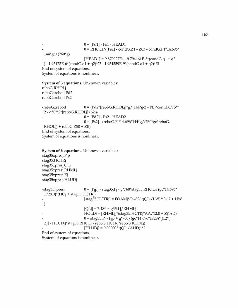
163

- 0 = [Pd1] - Ps1 - HEAD1 - 0 = RHOL1*([Ps1] - condG.Z1 - ZC) - condG.P1*14.696* 144*gc/(760*g) - [HEAD1] = 9.870927E1 - 9.794161E-3*(condG.q1 + q2 ) - 1.95175E-6*(condG.q1 + q2)**2 - 1.954559E-9*(condG.q1 + q2)**3 End of system of equations. System of equations is nonlinear. System of 3 equations. Unknown variables: reboG.RHOLj reboG::reboil.Pd2 reboG::reboil.Ps2 -reboG::reboil 0 = (Pd2*[reboG.RHOLj]*g/(144*gc) - PB)*contrl.CV5** 2 - q50**2*[reboG.RHOLj]/62.4 - 0 = [Pd2] - Ps2 - HEAD2 - 0 = [Ps2] - (reboG.Pj*14.696*144*g/(760*gc*reboG. RHOLj) + reboG.Z50 + ZB) End of system of equations. System of equations is nonlinear. System of 6 equations. Unknown variables: stag35::presj.Pjp stag35.HCTRj stag35::presj.QLj stag35::presj.RHMLj stag35::presj.Zj stag35::presj.HLUDj -stag35::presj 0 = [Pjp] - stag35.Pj - g*760*stag35.RHOLj/(gc*14.696* 1728.0)*(HOj + stag35.HCTRj) - [stag35.HCTRj] = FOAMj*(0.4896*(QLj/LW)**0.67 + HW ) - [QLj] = 7.48*stag35.Lj/RHMLj - HOLDj = [RHMLj]*(stag35.HCTRj*AA/12.0 + Zj*AD) - 0 = stag35.Pj - Pjp + g*760/(gc*14.696*1728)*((12*[ Zj] - HLUDj)*stag35.RHOLj - reboG.HCTRj*reboG.RHOLj) - [HLUDj] = 0.000003*(QLj/AUD)**2 End of system of equations. System of equations is nonlinear.

164

APPENDIX C: ACSL CODE FOR SIMPLE DISTILLATION

COLUMN MODEL

PROGRAM ACSL simplified distillation -- distsim.csl 6/10/92 "Contains distgbh.dym 3/30/92 with alternate eqlbm" "3 stages (3,5,21) added 4/3/92" "large scale simplification of l-v eqlbm and vapor flow, elimination" " of virial equation as eq of state, 9 stages used " " (1,2,3,4,5,21,35,49,50), elimination of all " " algebraic loops." "Because of the use of submodels (MACROs), a full 50 stage model would" " mearly require additional stage(...) statements in the DERIVATIVE" " section of this program. " "--------------------------------------------------------------------" "------------Variable and constant definintion-----------------------" " AA Active area of sieve plate. Constant. (ft2)" " AD Downcomer crossectional area. Constant. (ft2)" " AH(j) Area of holes in sieve plate j. Constants. (ft2)" " ailg=2 Gear's method of integration " " ALPHA Factor to account for temperature drop across condenser. " " Constant. (ft2)" " ALPHji Molar volume of component i in the liquid phase of " " stage j. (cm3/gmol)" " AN Nominal Area of sieve plate. Constant. (ft2)" " ANT(a,i) Antoine constants A,B,C for component i. Constants" " Apc Area of condenstation heat transfer in the condenser.

Constant. (ft2)" " Apmr Area of boiling heat transfer in the reboiler. Constant. " " (ft2)" " As Area of steam condensation in the reboiler. Constant. (ft2)" " AT Tower corss sectional area. Constant. (ft2)" " AUD Area under downcomer. Constant. (ft2)" " Aw Area of heat transfer from cooling water to condenser tube wall.

Constant. (ft2)" " Ccw Cooling water heat capacity. Constant. (BTU/lb °R)" " Cdd Vena contracta coefficient for flow over wier. (-)" " CIk kth controller input. (mA/min)" " cinterval communication interval " " CISPk kth controller set point translated to (mA/min)" " Cmc Heat capacity of condenser tubes. Constant. (BTU/lb °R)" " Cmr Heat capacity of reboiler tubes. Constant. (BTU/lb °R)" " COk kth controller output to valves. (mA/min)" " CS4 Control valve position for steam flow (valve 4). (in2/hr)" " Csc Heat capacity of steam in reboiler tubes. (BTU/lb °R)" " CSCO Coefficients used to determine CS4." " CVkCO coefficients used to determine CVk" " Cvc Vena contracta coefficient for a circular hole. (-)" " CVk kth control valve position for liquid flow. (gal/min

lb/in2 )" " Cx Vena contract coefficient for flow from downcomer. (-)" " DH Sieve plate hole diameter. Constant."

165

" dQVj Total change in vapor flow through sieve plate. (ft2)" " DR Diameter of the distillate receiver. Constant. (ft)" " DTT Tower diameter. Constant. (ft)" " Ej Holdup of enthalpy in liquid phase of stage j. (BTU)" " ETTA(i,k) Cross self-interaction parameter. Constants. (-)" " EVj Enthalpy of vapor flow leaving stage j. (BTU/min)" " F Feed rate. Constants. (mol/min)" " FOAMj Froth density correction factor. (-)" " FVAj Factor related to kinetic energy of vapor leaving stage j. "

" (ft. lb/ft3 /sec)" " g Acceleration of gravity. Constant. (ft/min2)" " HCTRj Equivalent height of clear liquid on the sieve plate " " of stage j. (ft)" " Hf Enthalpy of the feed to stage j. constant. (BTU/min)" " hLCO(i) Coefficients to determine enthalpy of liquid, hLji." " HLDPj Total liquid mass on stage j. (mol)" " hLji Partial molar enthalpy of component i in liquid phase " " of stage j. (BTU/mol)" " hLSC Enthalpy of saturated condensate (water) leaving the " " reboiler. (BTU/lb)" " hLSCO Coefficients used to determine hLSC." " howj Height of foam over the wier on stage plate j. (ft)" " HSH Enthalpy in the steam header. Constant. (BTU/lb)" " HVCO Vapor enthalpy coefficients used for HVji. Constants" " HVji Partial molar enthalpy of component i in vapor phase of " " stage j. In this model, ideal gas is assumed. (BTU/mol)" " HVSC Enthalpy of saturated steam in the reboiler. (BTU/lb)" " HVSCO coefficients for HVSC." " HW Height of the weir of sieve plate j. Constant. (in)" " HWSP Height of the weir of the seal pan (stage 50). " " Constant (in)" " Ik Sum of the integral of the error and the steady-state bias " " for contoller k. (mA)" " jm postscript denoting stage j-1" " jp postscript denoting stage j+1" " Kji Ideal equilibrium ratio (K-value) for component i on stage j." " LH Thickness of sieve plate. Constant. (ft)" " Lj Total molar flow rate of liquid leaving stage j. (mol/min)" " LR Length of the receiver. constant. (ft)" " Lspj Total molar flow rate of liquid leaving seal pan. (mol/min)" " LW Length of the weir of sieve plates. Constant. (in)" " LWSP Length of the seal pan weir. (in)" " merror relative error of state variables" " MOL Molecular weight of component i. Constants. (lb/mol)" " MOLV Weighted average of vapor molecular weight. (lb/mol)" " MV Molar volume coefficients for liquid. " " nstps initial # of steps per cint " " PB Pressure downstream of bottom product control valve. " " Constant. (lb/in2)" " PC Critial pressure for component i. Constants. (atm)" " PCC Cross critical pressure of components i and k. constants.

(atm)" " PD Pressure downstream of overhead product control valve.

Constant.(lb/in2)" " Pd1 Discharge pressure of pump 1" " Pd2 Discharge pressure of pump 2" " Pj Pressure of stage j (lb/in2)" " PDD Average of PD and P2 “

166

" pii π" " Pke Pressure drop across sieve plate due to kinetic energy of

vapor. (lb/in2)" " Ps1 Suction pressure of pump 1" " Ps2 Suction pressure of pump 2" " PSH Steam pressure upsteam of steam control valve. (lb/in2)" " PSji Saturation pressure (vapor pressure) of liquid phase of " " component i as predicted by Antone's equation. (mmHg)" " PUD Pressure drop under the downcomer. (ft)" " Pw1 Cooling tower pressure upstream of control valve. Constant. " " (lb/in2)" " Pw2Pw3 Reference pressure drop across condenser. (lb/in2)" " Pw3 Cooling water pressure downstream of condenser. (lb/in2)" " q1 Volume flow of reflux. (gal/min)" " q2 Volume flow of overhead product (distillate). (gal/min)" " QC Condenser duty, heat flow to condenser. (BTU/min)" " Qcw Volume flow of cooling water. (gal/min)" " Qcwo Reference volume flow of cooling water. (gal/min)" " QLj Volume flow of liquid leaving stage j. (ft3/min)" " QR Reboiler duty, heat flow from reboiler. (BTU/min)" " Qsj Volume flow of liquid over the weir of stage j. (ft3/min)" " R Reflux ratio." " RECVOL(Zj) Receiver volume function. (ft3)" " REF2 Reference pressure drop across condenser. (lb/in2)" " REF3 Reference pressure drop across condenser divided by the " " product of vapor molar flow into the condenser and vapor" " mass density. Constant. (ft min2/mol)" " RHMLj Molar density of liquid of stage j. (mol/ft3)" " RHMVj Molar density of vapor of stage j. (mol/ft3)" " RHOLj Mass density of liquid of stage j. (lb/ft3)" " RHOSC Mass density of saturated steam in the reboiler. (mol/ft3)" " RHOSCO Coefficients used to determine RHOSC." " RHOVj Mass density of vapor of stage j. (lb/ft3)" " RR Gas constant. (Various units, depending on use)" " SP Set Points of the 5 variables controlled: " " P1(mmHg), q2(gal/min), Z1(ft), (), Z50(ft), T35(R)" " sumvj Molar vapor flow leaving stage j. (mol/min) " " TAUI time constants of Integrator in 6 PI controllers, " " constants. (min)" " TAUM time constant of the temperature sensor. (min)" " TAUV time constants of 6 control Valves, constants. (min)" " TC Critical temperature of component i. (°R)" " TCC Cross-critical temperature of component i. (°R)" " Tj Temperature of liquid and vapor leaving stage j. (°R)" " TKj Temperature in Kelvin." " Tmc Temperature of condenser tubes. (°R)" " Tmr Temperature of reboiler tubes. (°R)" " tmx Max time of simulation (min.) " " TR Reduced temperature, except is has funny dimensions. (°R/°K)" " TRR Reduced temperature. (-)" " TSAT Saturated temperature of steam at header pressure. " " Constant. (°R)" " Tsc Temperature of steam in reboiler tubes. (°R)" " TSH Temperature of super-heated steam in the steam header.

Constant. (°R)" " TT Sieve plate thickness. Constant. (in)"

167

" Twi Temperature of cooling water entering condenser. Constant. (°R)"

" Two Temperature of cooling water leaving condenser. (°R)" " Ucw Holdup of cooling water in condenser. Constant. (lb)" " UHj Velocity of vapor in the holes of the stage j sieve plate. " " (ft/sec)" " uji Molar holdup of component i liquid of stage j. (mol)" " Umc Mass of tube metal in condenser. Constant. (lb)" " Umr Mass of tube metal in reboiler. Constant. (lb)" " Upmo Reference heat transfer film coefficient between process " " and condenser tube wall. Constant. (BTU/hr ft2 °R)" " Upmr Boiling film coefficient in reboiler. Constant. " " (BTU/hr ft2 °R)" " Us Reboiler steam side condensing film coefficient. Constant. " " (BTU/hr ft2 °R)" " UVj Molar vapor holdup on stage j. Constants. (mol)" " UVAj Velocity of vapor leaving stage j. (ft/sec)" " Uwmo Reference heat transfer film coefficient between cooling " " water and condenser tube wall. Constant. (BTU/hr ft2 °R)" " VC Critical volume of component i. Constants. (cm2/gmol)" " Vdc Volume of liquid in stage j downcomer. (ft3)" " vji Molar flow of component i from stage j as vapor. (mol/min)" " VOLBTW Volume of liquid in the tower base. (ft3)" " VOLREC Volume of liquid in the receiver. (ft3)" " Vr Volume of steam side of reboiler. (ft3)" " Wsh Steam flow to the reboiler. (lb/min)" " X,Y,Z Intermediate values used to determine Pd1." " XKC proportional gain in 6 PI controllers, constants" " Yji Molar fraction of component i in vapor. (-)" " ZB Vertical distance from column base to pump 2. Constant. (ft)" " ZC Vertical distance from bottom of receiver to pump 1. Constant.

(ft)" " ZETAk kth control valve position. (mA)" " Zj Height of equivalent clear liquid in the downcomer of stage j.

(ft)" "------------------ACSL program control variables" tmx = 60.0 cinterval cint=1.0 algorithm ailg=2 nsteps nstps=1000 minterval mint=0.0001 maxterval maxt=5.0 merror u22=1.E-5, T1=1.E-7, T50=1.E-7, z97377=1.E-3,Z98533=1.E-3, ... Z98827=1.E-3, Z99121=1.E-3, E1=7.E-7, E2=8.E-6, E3=9.E-6, ... E4=8.E-6, E5=5.E-6, E21=5.E-6 ,E35=5.E-6, E49=7.E-6 "-----Initial Values" constant E01=903324.0, E02=70279.2, E03=74348.1, ... E04=98215., E05=250686, E021=251678., ... E035=249803., E049=267101., E050=9950470. constant T01=598.770, T02=609.211, T03=616.34, ... T04=627.371, T05=639.640, T021=640.197, ... T035=641.159, T049=643.617, T050=644.693 constant Z01=3.0, Z02=.374189, Z03=.331997, ... Z04=.455558, Z05=1.09806, Z021=1.08924, ...

168

Z035=1.06254, Z049=1.13209, Z050=8. constant Qs01=65.518, Qs02=59.4878, Qs03=51.2026, ... Qs04=42.4723, Qs05=194.664, Qs021=193.908, ... Qs035=191.331, Qs049=185.191, Qs050=169.196 constant how02=.0941719, how03=.0814453, ... how04=.0709429, how05=.206904, how021=.20602, ... how035=.204584, how049=.200172, how050=.184973 constant hcl02=.105436, hcl03=.0977002, ... hcl04=.0914545, hcl05=.172059, hcl021=.171555, ... hcl035=.170726, hcl049=.168104 constant u101=221.458, u201=126.773, u301=8.33504, ... u401=8.26399, ... u102=16.2189, u202=6.96898, u302=1.06823, u402=2.47162, ... u103=14.3473, u203=5.37857, u303=1.38011, u403=6.51095, ... u104=13.3136, u204=4.96873, u304=1.6149, u404=14.9326, ... u105=20.8692, u205=7.96256, u305=3.00135, u405=53.5029, ... u1021=20.8436, u2021=7.79217, u3021=3.03287, u4021=53.7695, ... u1035=20.382, u2035=7.37883, u3035=3.06659, u4035=54.2729, ... u1049=19.8538, u2049=6.89401, u3049=3.26108, u4049=59.5047, ... u1050=582.659, u2050=190.483, u3050=112.989, u4050=2496.92 constant ... v102=62.737, v202=35.9139, v302=2.36122, v402=2.34108, ... v103=61.8336, v203=28.9926, v303=3.59338, v403=7.46932, ... v104=53.9779, v204=23.5895, v304=4.19821, v404=17.4251, ... v105=43.2344, v205=19.5179, v305=3.82395, v405=30.0847, ... v1021=44.5776, v2021=19.6452, v3021=3.99251, v4021=31.1786, ... v1035=44.3349, v2035=18.839, v3035=4.11403, v4035=32.0323, ... v1049=42.4142, v2049=17.0497, v3049=4.28344, v4049=34.6156, ... v1050=35.5974, v2050=13.3416, v3050=4.41514, v4050=44.5073 constant I01=22.8315, I02=4.93478, I03=7.16095, I04=26.2638, ... I05=33.5039, I06=10.3385, ... ZET01=.463481, ZET02=.521059, ZET03=.406421, ... ZET04=0.734895, ZET05=.796989 constant Tmc0=579.767,Two0=566.222, ... Tmr0=739.522, Tsc0=764.402, Tm0=641.159 "----------controller set-points, gains, time-constants" TABLE SP, 1, 6 /... 1,2,3,4,5,6, 760, 490.135, 3.0, 0.0, 8.0, 641.161/ TABLE XKC,1,6/... 1,2,3,4,5,6,... 1.5, 0.25, 1.1, 0.15, 0.5, 0.5/ TABLE TAUI,1,6/... 1,2,3,4,5,6,... 3.0, 0.1, 0.75, 0.25, 1.0, 0.6/ TABLE TAUV,1,6/... 1,2,3,4,5,6,... 0.15, 0.15, 0.15, 0.2, 0.15, 0.15/ " Twi changed from 545.---6/5/92" INITIAL Constant... AA=141.372 , AD=17.6715 , ALPHA=0.2 , AN=141.372 , ... Apc=16022.16 , Apmr=3361.826 , As=3844.168 , AT=176.714 , ... AUD=0.908375 , Aw=13940.0 , Ccw=1.0 , Cmc=0.12 , ... Cmr=0.12 , Cvc = .65, Cx = .58, DH=0.1875, DR=10.0 , ... DTT=15.0 , g = 115523.24, HSH=1262.8 , HW=1.0 , ... HWSP=1.25 , LH = 0.0078125, LR=16.0 , LW=130.806 , ... LWSP=149.0 , PB=30 , PD=40 , pii=3.14159 , ...

169

PSH=255.0 , Pw1=60 , Pw2Pw3=9.0 , Pw3=35 , Qcwo=8653.0 , ... REF1 = 0.947775644, REF2 = 9.0, REF3=2.9659168, ... RHO2VR=0.002549852, sumv1 = 1.0, Sv2IR=105.8752 , ... TAUM=0.20 , TSAT=862.7 , TSH=960.0 , TT=0.09375 , ... Twi=530. , Ucw=17160.0 , Umc=45000.0 , Umr=11000.0, ... Upmo=213.0 , Upmr=300.0 , Us=1000.0 , Uwmo=1250.0 , ... Vr=68.83 , ZB=10.0 , ZC=5.0 "gravitational acceleration, g, in ft/min**2" "---------controller set points (in mA.) " CISP1 = 0.032*SP(1.0) - 12.0 CISP2 = (SP(2.0)/200)**2 + 4.0 CISP3 = 4.0 + 1.6*SP(3.0) CISP5 = -20.0 + 4*SP(5.0) CISP6 = 0.4*SP(6.0) - 236. "--------coeficients " TABLE MV, 2, 3, 4 /... 1,2,3, 1,2,3,4,... 0.6451094E2, -0.1095359 , 0.1195526E-3,... 0.5686523E2, 0.468039E-2, 0.5094978E-4,... 0.5370027E2, -0.1728176E-1, 0.493820E-4,... 0.2288676E2, -0.2023121E-1, 0.2115899E-4/ TABLE HVCO, 2, 5, 4/... 1, 2, 3, 4, 5, 1, 2, 3, 4,... 0.1174119E5, 0.7121495E1, 0.5579442E-2, ... -0.450617E-6, -0.2091904E-10,... 0.867332E4, 0.4735799E1, 0.1452860E-1,... -0.1121397E-5, -0.2018173E-9,... 0.106486E5, 0.7515997E1, 0.1151360E-1,... -.01682096E-5, 0.9036333E-10,... 0.1545871E5, 0.8022526E1, -0.4745722E-3,... 0.6878047E-6, -0.1439752E-9/ TABLE hLCO, 2, 3, 4/... 1, 2, 3, 1, 2, 3, 4,... -0.3119436E4, -4.145198, 0.2131106E-1, ... -0.115334E5, 0.1770348E2, 0.1166435E-1, ... 0.4046348E3, -0.2410286E2, 0.472823E-1, ... -0.87838059E4, 0.175845E2, 0.3651369E-3/ TABLE ANT, 2, 3, 4/... 1,2,3, 1,2,3,4,... 7.87863, 1.47311E3, 2.3E2,... 7.02447, 1.16E3, 2.24E2,... 8.04494, 1.5543E3, 2.2265E2,... 7.96681, 1.66821E3,2.28E2/ TABLE WLMB,2,4,4/... 1,2,3,4, 1,2,3,4,... 0.0, 0.66408E3, 0.59844E3, 0.20530E3,... -0.21495E3, 0.0, 0.38170E2, 0.43964E3,... 0.51139E3, 0.41896E3, 0.0, 0.38230E3,... 0.48216E3, 0.140549E3, 0.95549E3, 0.0/ TABLE RHOSCO, 1, 5/... 1,2,3,4,5,... 1.031951E-2, 1.427797E1, 0.9414444, 2.048037, 5.956991/ TABLE hLSCO, 1, 5/... 1,2,3,4,5,... -1.6029E2, 8.06427E-2, 7.361453E-5, 1.501012E-6,... -9.9964334E-10/ TABLE HVSCO, 1, 5/... 1,2,3,4,5,...

170

5.448738E2, 8.039637E-1, 1.931794E-3, -3.938661E-6,... 1.907853E-9/ TABLE HEDCO, 2,4,2/... 1,2,3,4, 1,2,... 9.870927E1, -9.794161E-3, -1.95175E-6, -1.954559E-9,... 9.152028E1, -6.584299E-2, 7.533832E-5, -4.300139E-8/ TABLE CV1CO , 2, 5, 20/... 1,2,3,4,5,... 0.0,0.099,0.1,0.19,0.2,0.29,0.3,0.39,0.4,0.49,... 0.5,0.59,0.6,0.69,0.7,0.79,0.8,0.89,0.9,1.0,... 0.0, 0.0, 0.6759999E2, -0.6691973E3, 0.6691969E4,... 0.0, 0.0, 0.6759999E2, -0.6691973E3, 0.6691969E4,... 0.1, 0.676E1, 0.1345197E3, -0.1167920E4, 0.8667223E4,... 0.1, 0.676E1, 0.1345197E3, -0.1167920E4, 0.8667223E4,... 0.2, 0.5810001E2, 0.9598074E3, -7506973E4, 0.8598887E5,... 0.2, 0.5810001E2, 0.9598074E3, -7506973E4, 0.8598887E5,... 0.3, 0.165E3, .2038081E4, -0.768066E4, 0.8299831E5,... 0.3, 0.165E3, .2038081E4, -0.768066E4, 0.8299831E5,... 0.4, 0.375E3, 0.2991901E4, -0.6826715E4, 0.4807690E5,... 0.4, 0.375E3, 0.2991901E4, -0.6826715E4, 0.4807690E5,... 0.5, 0.654E3, 0.3068865E4, -0.5726895E4, 0.6382414E4,... 0.5, 0.654E3, 0.3068865E4, -0.5726895E4, 0.6382414E4,... 0.6, 0.91E3, 0.2114958E4, -0.2852868E5, 0.2237909E6,... 0.6, 0.91E3, 0.2114958E4, -0.2852868E5, 0.2237909E6,... 0.7, 0.106E4, 0.3122954E4, 0.1411841E5, -0.9347956E5,... 0.7, 0.106E4, 0.3122954E4, 0.1411841E5, -0.9347956E5,... 0.8, 0.142E4, 0.3142248E4, -0.2419347E5, 0.1177098E6,... 0.8, 0.142E4, 0.3142248E4, -0.2419347E5, 0.1177098E6,... 0.9, 0.161E4, 0.1834851E4, -0.6969128E3, 0.3484387E4,... 0.9, 0.161E4, 0.1834851E4, -0.6969128E3, 0.3484387E4/ TABLE CV2CO, 2, 5, 20/... 1,2,3,4,5,... 0.0,0.099,0.1,0.19,0.2,0.29,0.3,0.39,0.4,0.49,... 0.5,0.59,0.6,0.69,0.7,0.79,0.8,0.89,0.9,1.0,... 0.0, 0.0, 0.6759999E2, -0.6691973E3, 0.6691969E4,... 0.0, 0.0, 0.6759999E2, -0.6691973E3, 0.6691969E4,... 0.1, 0.676E1, 0.1345197E3, -0.1167920E4, 0.8667223E4,... 0.1, 0.676E1, 0.1345197E3, -0.1167920E4, 0.8667223E4,... 0.2, 0.172E2, 0.1609525E3, -0.5040024E3, 0.5344770E4,... 0.2, 0.172E2, 0.1609525E3, -0.5040024E3, 0.5344770E4,... 0.3, 0.3360001E2, 0.2204954E3, -0.1038741E4, 0.8337859E4,... 0.3, 0.3360001E2, 0.2204954E3, -0.1038741E4, 0.8337859E4,... 0.4, 0.5360001E2, 0.2628831E3, -0.9942312E3, 0.8153996E4,... 0.4, 0.5360001E2, 0.2628831E3, -0.9942312E3, 0.8153996E4,... 0.5, 0.7810001E2, 0.3086567E3, -0.1381982E4, 0.1085412E5,... 0.5, 0.7810001E2, 0.3086567E3, -0.1381982E4, 0.1085412E5,... 0.6, 0.106E3, 0.3578840E3, -0.1145935E4, 0.8670914E4,... 0.6, 0.106E3, 0.3578840E3, -0.1145935E4, 0.8670914E4,... 0.7, 0.139E3, 0.3888247E3, -0.1526535E4, 0.1038285E5,... 0.7, 0.139E3, 0.3888247E3, -0.1526535E4, 0.1038285E5,... 0.8, 0.173E3, 0.3950034E3, -0.6824436E3, 0.2324071E4,... 0.8, 0.173E3, 0.3950034E3, -0.6824436E3, 0.2324071E4,... 0.9, 0.208E3, 0.3282368E3, -0.1564725E4, 0.7823613E4,... 0.9, 0.208E3, 0.3282368E3, -0.1564725E4, 0.7823613E4/ TABLE CV3CO, 2, 5, 20/... 1,2,3,4,5,... 0.0,0.099,0.1,0.19,0.2,0.29,0.3,0.39,0.4,0.49,... 0.5,0.59,0.6,0.69,0.7,0.79,0.8,0.89,0.9,1.0,... 0.0, 0.0, 0.6689999E2, -0.17743E3, 0.1742997E4,... 0.0, 0.0, 0.6689999E2, -0.17743E3, 0.1742997E4,... 0.1, 0.669E1, 0.8432991E2, -0.8532524E3, 0.5009532E4,...

171

0.1, 0.669E1, 0.8432991E2, -0.8532524E3, 0.5009532E4,... 0.2, 0.116E2, 0.6396542E2, -0.3343521E3, 0.3846974E4,... 0.2, 0.116E2, 0.6396542E2, -0.3343521E3, 0.3846974E4,... 0.3, 0.185E2, 0.1125043E3, -0.6310693E3, 0.6060258E4,... 0.3, 0.185E2, 0.1125043E3, -0.6310693E3, 0.6060258E4,... 0.4, 0.295E2, 0.1680985E3, -0.9577654E3, 0.9167789E4,... 0.4, 0.295E2, 0.1680985E3, -0.9577654E3, 0.9167789E4,... 0.5, 0.4589999E2, 0.2515793E3, -0.132549E4, 0.1269696E5,... 0.5, 0.4589999E2, 0.2515793E3, -0.132549E4, 0.1269696E5,... 0.6, 0.705E2, 0.3673904E3, -0.1754303E4, 0.1630397E5,... 0.6, 0.705E2, 0.3673904E3, -0.1754303E4, 0.1630397E5,... 0.7, 0.106E3, 0.5056489E3, -0.2605563E4, 0.2349071E5,... 0.7, 0.106E3, 0.5056489E3, -0.2605563E4, 0.2349071E5,... 0.8, 0.154E3, 0.6892578E3, -0.2990246E4, 0.2697664E5,... 0.8, 0.154E3, 0.6892578E3, -0.2990246E4, 0.2697664E5,... 0.9, 0.22E3, 0.9005083E3, -0.1210117E4, 0.6050512E4,... 0.9, 0.22E3, 0.9005083E3, -0.1210117E4, 0.6050512E4/ TABLE CV5CO, 2, 5, 20/... 1,2,3,4,5,... 0.0,0.099,0.1,0.19,0.2,0.29,0.3,0.39,0.4,0.49,... 0.5,0.59,0.6,0.69,0.7,0.79,0.8,0.89,0.9,1.0,... 0.0, 0.0, 0.463E3, -0.3610995E4, 0.3610991E5,... 0.0, 0.0, 0.463E3, -0.3610995E4, 0.3610991E5,... 0.1, 0.463E2, 0.8240989E3, -0.5206883E4, 0.3035894E5,... 0.1, 0.463E2, 0.8240989E3, -0.5206883E4, 0.3035894E5,... 0.2, 0.107E3, 0.6934902E3, -0.1574331E4, 0.1039425E5,... 0.2, 0.107E3, 0.6934902E3, -0.1574331E4, 0.1039425E5,... 0.3, 0.171E3, 0.6904519E3, -0.2672921E4, 0.1468400E5,... 0.3, 0.171E3, 0.6904519E3, -0.2672921E4, 0.1468400E5,... 0.4, 0.228E3, 0.5963877E3, -0.2192055E4, 0.1328175E5,... 0.4, 0.228E3, 0.5963877E3, -0.2192055E4, 0.1328175E5,... 0.5, 0.279E3, 0.5564294E3, -0.1604116E4, 0.8398187E4,... 0.5, 0.279E3, 0.5564294E3, -0.1604116E4, 0.8398187E4,... 0.6, 0.327E3, 0.4875520E3, -0.1870622E4, 0.9950992E4,... 0.6, 0.327E3, 0.4875520E3, -0.1870622E4, 0.9950992E4,... 0.7, 0.367E3, 0.4119575E3, -0.4696677E3, -0.1499096E4,... 0.7, 0.367E3, 0.4119575E3, -0.4696677E3, -0.1499096E4,... 0.8, 0.402E3, 0.2730510E3, -0.1572119E4, 0.6416082E4,... 0.8, 0.402E3, 0.2730510E3, -0.1572119E4, 0.6416082E4,... 0.9, 0.42E3, 0.1511098E3, -0.4221873E3, 0.2110922E4,... 0.9, 0.42E3, 0.1511098E3, -0.4221873E3, 0.2110922E4/ TABLE CSCO , 2, 5, 20/... 1,2,3,4,5,... 0.0,0.099,0.1,0.19,0.2,0.29,0.3,0.39,0.4,0.49,... 0.5,0.59,0.6,0.69,0.7,0.79,0.8,0.89,0.9,1.0,... 0.0, 0.0, 0.112E3, -0.280999E3, 0.2809984,... 0.0, 0.0, 0.112E3, -0.280999E3, 0.2809984,... 0.1, 0.193E2, 0.9875446E2, -0.6029138E3, 0.6653684E4,... 0.1, 0.193E2, 0.9875446E2, -0.6029138E3, 0.6653684E4,... 0.2, 0.193E2, 0.9875446E2, -0.6029138E3, 0.6653684E4,... 0.2, 0.193E2, 0.9875446E2, -0.6029138E3, 0.6653684E4,... 0.3, 0.298E2, 0.1777826E3, -0.8587102E3, 0.8508832E4,... 0.3, 0.298E2, 0.1777826E3, -0.8587102E3, 0.8508832E4,... 0.4, 0.475E2, 0.2613057E3, -0.1764654E4, 0.1651596E5,... 0.4, 0.475E2, 0.2613057E3, -0.1764654E4, 0.1651596E5,... 0.5, 0.725E2, 0.4038538E3, -0.2260444E4, 0.2271903E5,... 0.5, 0.725E2, 0.4038538E3, -0.2260444E4, 0.2271903E5,... 0.6, 0.133E3, 0.6333362E3, -0.2353483E4, 0.2220118E5,... 0.6, 0.133E3, 0.6333362E3, -0.2353483E4, 0.2220118E5,... 0.7, 0.175E3, 0.8286753E3, -0.2622047E4, 0.1935291E5,... 0.7, 0.175E3, 0.8286753E3, -0.2622047E4, 0.1935291E5,...

172

0.8, 0.251E3, 0.8848535E3, -0.6906321E3, -0.4579047E4,... 0.8, 0.251E3, 0.8848535E3, -0.6906321E3, -0.4579047E4,... 0.9, 0.328E3, 0.6093555E3, -0.4187094E4, 0.2093548E5,... 0.9, 0.328E3, 0.6093555E3, -0.4187094E4, 0.2093548E5/ "--------Physical constants " TABLE PCC, 2, 4, 4/... 1,2,3,4, 1,2,3,4,... 78.5, 59.6, 70.0, 127.8,... 59.6, 46.6, 54.0, 93.5,... 70.0, 54.0, 63.0, 111.9,... 127.8, 93.5, 111.9, 218.3/ TABLE TCC, 2, 4, 4/... 1,2,3,4, 1,2,3,4,... 513.2, 510.9, 514.1, 576.4,... 510.9, 508.7, 512.3, 573.9,... 514.1, 512.3, 516.0, 578.0,... 576.4, 573.9, 578.0, 647.4/ TABLE TC,1,4/... 1,2,3,4,... 513.2, 508.7, 516.0, 647.4/ TABLE PC,1,4/... 1,2,3,4,... 78.5, 46.6, 63.0, 218.3/ TABLE VC,1,4/... 1,2,3,4,... 118.0, 213.5, 161.3, 55.2/ TABLE WW,1,4/... 1,2,3,4,... 0.557, 0.309, 0.637, 0.344/ TABLE WWH,1,4/... 1,2,3,4,... 0.105, 0.187, 0.152, 0.010/ TABLE MU,1,4/... 1,2,3,4,... 1.66, 2.88, 1.69, 1.83/ TABLE ETTA, 2,4,4/... 1,2,3,4, 1,2,3,4,... 1.21, 0.605, 1.155, 0.605,... 0.605, 0.0, 0.55, 0.0,... 1.155, 0.55, 1.1, 0.55,... 0.605, 0.0, 0.55, 0.0/ TABLE MUR, 2, 4, 4/... 1,2,3,4 ,1,2,3,4,... 4.408, 4.693, 4.308, 4.761,... 4.693, 5.006, 4.607, 5.008,... 4.308, 4.607, 4.213, 4.640,... 4.761, 5.008, 4.640, 5.161/ TABLE WH, 2, 4, 4/... 1,2,3,4, 1,2,3,4,... 0.105, 0.146, 0.1285, 0.0575,... 0.146, 0.187, 0.1695, 0.0985,... 0.1285, 0.1695, 0.152, 0.081,... 0.0575, 0.0985, 0.081, 0.01/ TABLE MOL, 1, 4/... 1,2,3,4,... 32.04,58.08,46.07,18.016/ "------------Column constants and forcing functions " TABLE AH, 1, 4/... 1,3,4,50,... 18,18,13,13/ TABLE CD, 1, 4/...

173

1, 3, 4, 50,... 0.75, 0.75, 0.72, 0.72/ TABLE F, 2, 10, 4/... 1,2,3,4,5,6,20,21,22,50,... 1,2,3,4,... 0., 0., 0., 0., 65.25, 0.,0., .0, 0., 0., ... 0., 0., 0., 0., 25.5, 0., 0., .0, 0., 0., ... 0., 0., 0., 0., 10.0, 0., 0., .0, 0., 0., ... 0., 0., 0., 0., 207.5, 0., 0., .0, 0., 0./ TABLE Hf, 1, 10/... 1,2,3,4,5,6,20,21,22,50,... 0.0, 0.0, 0.0, 0.0, 868000., 0.0, ... 0.0, 0.0, 0.0, 0.0/ "-----Receiver liquid height to volume function" TABLE RECVOL, 1, 27/... 0.0,2.12692,5.99764,10.9848,16.8604,23.4904,42.8183,... 65.4004,90.6624,118.2,178.918,245.674,317.069,391.969,... 469.392,548.452,628.319,708.185,787.245,864.668,939.568,... 1010.96,1077.72,1138.44,1191.24,1233.15,1256.64,... 0.0,0.1,0.2,0.3,0.4,0.5,0.75,1.0,1.25,1.5,2.0,2.5,3.0,... 3.5,4.0,4.5,5.0,5.5,6.0,6.5,7.0,7.5,8.0,8.5,9.0,9.5,10.0/ "UV(1) changed from 2.1557724" TABLE UV, 1, 9/... 1,2,3,4,5,21,35,49,50,... 2.15, 2.00531, 1.9955679, 1.965454, 1.8892558, ... 1.9032513, 1.91708, 1.92265, 2.0345702/ "-----Gas Constant in atm*ft**3/lBmol*K, cm**3*mmHg/gmol*K," " ft**3*mmHg/lBmol*R, cal/gmol*K, lb*ft**3/ft**2*lBmol*R" TABLE RR, 1, 5/... 1,2,3,4,5,... 1.314, 62361.0, 555.0, 1.987, 1545.0/ "------------------------Energy models-------------------------------" MACRO engb1(Tj, TKj, R, QC, Ej, Lj, HLDPj, EVjp, ... uj1, uj2, uj3, uj4, duj1,duj2,duj3,duj4, J) MACRO Redefine Ejdot, jj, dTj, hLj1,hLj2,hLj3,hLj4 jj = J/1.0 Ejdot = Hf(jj) + EVjp - (1 + R)*Lj*Ej/(R * HLDPj) - QC Ej = INTEG(Ejdot, E0&J) hLj1 = hLCO(1.0,1.0) + hLCO(2.0,1.0)*Tj + hLCO(3.0,1.0)*Tj**2 hLj2 = hLCO(1.0,2.0) + hLCO(2.0,2.0)*Tj + hLCO(3.0,2.0)*Tj**2 hLj3 = hLCO(1.0,3.0) + hLCO(2.0,3.0)*Tj + hLCO(3.0,3.0)*Tj**2 hLj4 = hLCO(1.0,4.0) + hLCO(2.0,4.0)*Tj + hLCO(3.0,4.0)*Tj**2 Tj = INTEG(dTj, T0&J) TKj = 5.0*Tj/9.0 dTj = (Ejdot - hLj1*duj1 - hLj2*duj2 - hLj3*duj3 - hLj4*duj4)/ ... ((hLCO(2.0,1.0) + 2*hLCO(3.0,1.0)*Tj)*uj1 ... + (hLCO(2.0,2.0) + 2*hLCO(3.0,2.0)*Tj)*uj2 ... + (hLCO(2.0,3.0) + 2*hLCO(3.0,3.0)*Tj)*uj3 ... + (hLCO(2.0,4.0) + 2*hLCO(3.0,4.0)*Tj)*uj4) MACRO END MACRO engbj(Ej, Lj, Ljm, Ejm,uj1, uj2, uj3, uj4, ...

174

HLDPj, HLDPjm, duj1,duj2,duj3,duj4, EVj,EVjp, ... vj1,vj2,vj3,vj4,sumvj, Tj, TKj, J) MACRO Redefine Ejdot,jj, dTj, hLj1,hLj2,hLj3,hLj4, ... HVj1,HVj2,HVj3,HVj4 jj = J/1.0 Ejdot = Hf(jj) + Ljm*Ejm/HLDPjm - Lj*Ej/HLDPj + ... EVjp - EVj Ej = INTEG(Ejdot, E0&J) HVj1 = HVCO(1.0,1.0) + HVCO(2.0,1.0)*Tj + HVCO(3.0,1.0)*Tj**2 + ... HVCO(4.0,1.0)*Tj**3 + HVCO(5.0,1.0)*Tj**4 HVj2 = HVCO(1.0,2.0) + HVCO(2.0,2.0)*Tj + HVCO(3.0,2.0)*Tj**2 + ... HVCO(4.0,2.0)*Tj**3 + HVCO(5.0,2.0)*Tj**4 HVj3 = HVCO(1.0,3.0) + HVCO(2.0,3.0)*Tj + HVCO(3.0,3.0)*Tj**2 + ... HVCO(4.0,3.0)*Tj**3 + HVCO(5.0,3.0)*Tj**4 HVj4 = HVCO(1.0,4.0) + HVCO(2.0,4.0)*Tj + HVCO(3.0,4.0)*Tj**2 + ... HVCO(4.0,4.0)*Tj**3 + HVCO(5.0,4.0)*Tj**4 hLj1 = hLCO(1.0,1.0) + hLCO(2.0,1.0)*Tj + hLCO(3.0,1.0)*Tj**2 hLj2 = hLCO(1.0,j + HVCO(3.0,1.0)*Tj**2 + ... HVCO(4.0,1.0)*Tj**3 + HVCO(5.0,1.0)*Tj**4 HVj2 = HVCO(1.0,2.0) + HVCO(2.0,2.0)*Tj + HVCO(3.0,2.0)*Tj**2 + ... HVCO(4.0,2.0)*Tj**3 + HVCO(5.0,2.0)*Tj**4 HVj3 = HVCO(1.0,3.0) + HVCO(2.0,3.0)*Tj + HVCO(3.0,3.0)*Tj**2 + ... HVCO(4.0,3.0)*Tj**3 + HVCO(5.0,3.0)*Tj**4 HVj4 = HVCO(1.0,4.0) + HVCO(2.0,4.0)*Tj + HVCO(3.0,4.0)*Tj**2 + ... HVCO(4.0,4.0)*Tj**3 + HVCO(5.0,4.0)*Tj**4 hLj1 = hLCO(1.0,1.0) + hLCO(2.0,1.0)*Tj + hLCO(3.0,1.0)*Tj**2 hLj2 = hLCO(1.0,2.0) + hLCO(2.0,2.0)*Tj + hLCO(3.0,2.0)*Tj**2 hLj3 = hLCO(1.0,3.0) + hLCO(2.0,3.0)*Tj + hLCO(3.0,3.0)*Tj**2 hLj4 = hLCO(1.0,4.0) + hLCO(2.0,4.0)*Tj + hLCO(3.0,4.0)*Tj**2 EVj = vj1*HVj1 + vj2*HVj2 + vj3*HVj3 + vj4*HVj4 Tj = INTEG(dTj, T0&J) TKj = 5.0*Tj/9.0 dTj = (Ejdot - hLj1*duj1 - hLj2*duj2 - hLj3*duj3 - hLj4*duj4)/ ... ((hLCO(2.0,1.0) + 2*hLCO(3.0,1.0)*Tj)*uj1 ... + (hLCO(2.0,2.0) + 2*hLCO(3.0,2.0)*Tj)*uj2 ... + (hLCO(2.0,3.0) + 2*hLCO(3.0,3.0)*Tj)*uj3 ... + (hLCO(2.0,4.0) + 2*hLCO(3.0,4.0)*Tj)*uj4) MACRO END "-----------------------Material-balance models--------------------" MACRO matb1(uj1, uj2, uj3, uj4, HLDP1, ... vjp1, vjp2, vjp3, vjp4, sumvjp, ... duj1,duj2,duj3,duj4, R, Lj, J) MACRO Redefine jj

175

jj = J/1.0 duj1 = f(jj,1.0) - (1 + R)*Lj*uj1/(R * HLDP1) + vjp1 uj1 = INTEG(duj1, u10&J) duj2 = f(jj,2.0) - (1 + R)*Lj*uj2/(R * HLDP1) + vjp2 uj2 = INTEG(duj2, u20&J) duj3 = f(jj,3.0) - (1 + R)*Lj*uj3/(R * HLDP1) + vjp3 uj3 = INTEG(duj3, u30&J) duj4 = f(jj,4.0) - (1 + R)*Lj*uj4/(R * HLDP1) + vjp4 uj4 = INTEG(duj4, u40&J) HLDP1 = uj1 + uj2 + uj3 + uj4 MACRO END MACRO matbj(uj1, uj2, uj3, uj4, HLDPj,ujm1,ujm2, ujm3, ujm4, ... HLDPjm,vj1, vj2, vj3, vj4, sumvj, ... vjp1, vjp2, vjp3, vjp4, sumvjp, Lj, Ljm, ... duj1, duj2, duj3, duj4, J) MACRO Redefine jj jj = J*1.0/1.0 duj1 = f(jj,1.0) + Ljm*ujm1/HLDPjm - Lj*uj1/HLDPj - vj1 + vjp1 uj1 = INTEG(duj1, u10&J) duj2 = f(jj,2.0) + Ljm*ujm2/HLDPjm - Lj*uj2/HLDPj - vj2 + vjp2 uj2 = INTEG(duj2, u20&J) duj3 = f(jj,3.0) + Ljm*ujm3/HLDPjm - Lj*uj3/HLDPj - vj3 + vjp3 uj3 = INTEG(duj3, u30&J) duj4 = f(jj,4.0) + Ljm*ujm4/HLDPjm - Lj*uj4/HLDPj - vj4 + vjp4 uj4 = INTEG(duj4, u40&J) HLDPj = uj1 + uj2 + uj3 + uj4 MACRO END MACRO matbN(uj1, uj2, uj3, uj4, HLDPj,ujm1,ujm2, ujm3, ujm4, ... HLDPjm,vj1, vj2, vj3, vj4, sumvj, ... duj1, duj2, duj3, duj4, Lj, Ljm, J) MACRO Redefine jj jj = J*1.0/1.0 duj1 = f(jj,1.0) + Ljm*ujm1/HLDPjm - Lj*uj1/HLDPj - vj1 uj1 = INTEG(duj1, u10&J) duj2 = f(jj,2.0) + Ljm*ujm2/HLDPjm - Lj*uj2/HLDPj - vj2 uj2 = INTEG(duj2, u20&J) duj3 = f(jj,3.0) + Ljm*ujm3/HLDPjm - Lj*uj3/HLDPj - vj3 uj3 = INTEG(duj3, u30&J) duj4 = f(jj,4.0) + Ljm*ujm4/HLDPjm - Lj*uj4/HLDPj - vj4 uj4 = INTEG(duj4, u40&J) HLDPj = uj1 + uj2 + uj3 + uj4 MACRO END "----------------------pressure models--------------------------" MACRO pres1(Pj, Pjp, Z1, RHMLj, HLDPj, sumvjp, Tj, ... vjp1,vjp2,vjp3,vjp4, Yjp1,Yjp2,Yjp3,Yjp4, J) MACRO Redefine VOLREC, RHMVj, efl1, efl2, efl3, efl4,dP Pj = RR(5.0)*Tj*RHMVj RHMVj = UV(1.0)/(1256.6 - VOLREC)

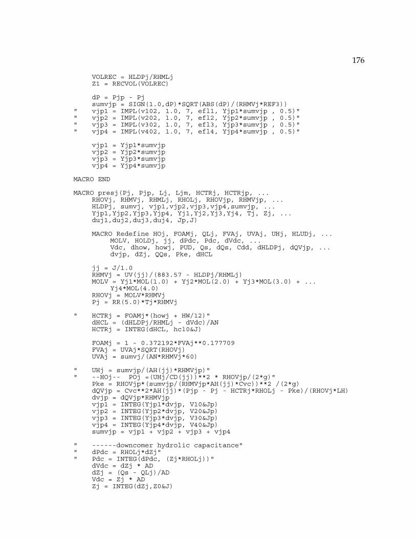
176

VOLREC = HLDPj/RHMLj Z1 = RECVOL(VOLREC) dP = Pjp - Pj sumvjp = SIGN(1.0,dP)*SQRT(ABS(dP)/(RHMVj*REF3)) " vjp1 = IMPL(v102, 1.0, 7, efl1, Yjp1*sumvjp , 0.5)" " vjp2 = IMPL(v202, 1.0, 7, efl2, Yjp2*sumvjp , 0.5)" " vjp3 = IMPL(v302, 1.0, 7, efl3, Yjp3*sumvjp , 0.5)" " vjp4 = IMPL(v402, 1.0, 7, efl4, Yjp4*sumvjp , 0.5)" vjp1 = Yjp1*sumvjp vjp2 = Yjp2*sumvjp vjp3 = Yjp3*sumvjp vjp4 = Yjp4*sumvjp MACRO END MACRO presj(Pj, Pjp, Lj, Ljm, HCTRj, HCTRjp, ... RHOVj, RHMVj, RHMLj, RHOLj, RHOVjp, RHMVjp, ... HLDPj, sumvj, vjp1,vjp2,vjp3,vjp4,sumvjp, ... Yjp1,Yjp2,Yjp3,Yjp4, Yj1,Yj2,Yj3,Yj4, Tj, Zj, ... duj1,duj2,duj3,duj4, Jp,J) MACRO Redefine HOj, FOAMj, QLj, FVAj, UVAj, UHj, HLUDj, ... MOLV, HOLDj, jj, dPdc, Pdc, dVdc, ... Vdc, dhow, howj, PUD, Qs, dQs, Cdd, dHLDPj, dQVjp, ... dvjp, dZj, QQs, Pke, dHCL jj = J/1.0 RHMVj = UV(jj)/(883.57 - HLDPj/RHMLj) MOLV = Yj1*MOL(1.0) + Yj2*MOL(2.0) + Yj3*MOL(3.0) + ... Yj4*MOL(4.0) RHOVj = MOLV*RHMVj Pj = RR(5.0)*Tj*RHMVj " HCTRj = FOAMj*(howj + HW/12)" dHCL = (dHLDPj/RHMLj - dVdc)/AN HCTRj = INTEG(dHCL, hcl0&J) FOAMj = 1 - 0.372192*FVAj**0.177709 FVAj = UVAj*SQRT(RHOVj) UVAj = sumvj/(AN*RHMVj*60) " UHj = sumvjp/(AH(jj)*RHMVjp)" " --HOj-- POj =(UHj/CD(jj))**2 * RHOVjp/(2*g)" Pke = RHOVjp*(sumvjp/(RHMVjp*AH(jj)*Cvc))**2 /(2*g) dQVjp = Cvc**2*AH(jj)*(Pjp - Pj - HCTRj*RHOLj - Pke)/(RHOVj*LH) dvjp = dQVjp*RHMVjp vjp1 = INTEG(Yjp1*dvjp, V10&Jp) vjp2 = INTEG(Yjp2*dvjp, V20&Jp) vjp3 = INTEG(Yjp3*dvjp, V30&Jp) vjp4 = INTEG(Yjp4*dvjp, V40&Jp) sumvjp = vjp1 + vjp2 + vjp3 + vjp4 " ------downcomer hydrolic capacitance" " dPdc = RHOLj*dZj" " Pdc = INTEG(dPdc, (Zj*RHOLj))" dVdc = dZj * AD dZj = (Qs - QLj)/AD Vdc = Zj * AD Zj = INTEG(dZj,Z0&J)

177

" --note that flows are allowed to become negative" QLj = Cx*AUD*SIGN(1.0,PUD)*SQRT(2*g*ABS(PUD)) PUD = (Pj - Pjp)/RHOLj - HCTRjp + Zj Lj = QLj*RHMLj " ------wier equations" dQs = Cdd*LW*dhow*SIGN(1.0,howj)*SQRT(2*g*ABS(howj))/12.0 QQs = INTEG(dQs, Qs0&J ) Qs = FCNSW(howj, 0.0, 0.0, QQs) Cdd = (1.368*(1.01 + .0063*(Qs*(12/LW)**2.5)))**1.5 dhow = (dHLDPj/RHMLj - dVdc)/(AN*FOAMj) dHLDPj = duj1 + duj2 + duj3 + duj4 howj = INTEG(dhow, how0&J ) MACRO END "-----------------------Liquid-Vapor equilibrium model------------" MACRO eql(uj1, uj2, uj3, uj4, HLDPj,Tj,TKj, ... Pj, Yj1, Yj2, Yj3, Yj4, RHMLj, RHOLj, J) MACRO Redefine PSj1, PSj2, PSj3, PSj4, Kj1, Kj2, Kj3 ,Kj4, ... ALPHj1, ALPHj2, ALPHj3, ALPHj4,sumK Yj1 = uj1*Kj1/sumK Yj2 = uj2*Kj2/sumK Yj3 = uj3*Kj3/sumK Yj4 = uj4*Kj4/sumK sumK = uj1*Kj1 + uj2*Kj2 + uj3*Kj3 + uj4*Kj4 Kj1 = PSj1/Pj ALPHj1 = MV(1.0,1.0) + MV(2.0,1.0)*Tj + MV(3.0,1.0)*Tj**2 PSj1 = 2.7855*10.**(ANT(1.0,1.0) - (ANT(2.0,1.0)/(ANT(3.0,1.0) + ... (TKj - 273.15)))) "--------------" Kj2 = PSj2/Pj ALPHj2 = MV(1.0,2.0) + MV(2.0,2.0)*Tj + MV(3.0,2.0)*Tj**2 PSj2 = 2.7855*10.**(ANT(1.0,2.0) - (ANT(2.0,2.0)/(ANT(3.0,2.0) + ... (TKj - 273.15)))) "--------------" Kj3 = PSj3/Pj ALPHj3 = MV(1.0,3.0) + MV(2.0,3.0)*Tj + MV(3.0,3.0)*Tj**2 PSj3 = 2.7855*10.**(ANT(1.0,3.0) - (ANT(2.0,3.0)/(ANT(3.0,3.0) + ... (TKj - 273.15)))) "-----------" Kj4 = PSj4/Pj ALPHj4 = MV(1.0,4.0) + MV(2.0,4.0)*Tj + MV(3.0,4.0)*Tj**2 PSj4 = 2.7855*10.**(ANT(1.0,4.0) - (ANT(2.0,4.0)/(ANT(3.0,4.0) + ... (TKj - 273.15)))) "---------" RHMLj = 62.43*HLDPj/(ALPHj1*uj1 +ALPHj2*uj2 + ... ALPHj3*uj3 + ALPHj4*uj4) RHOLj = 62.43*HLDPj/(ALPHj1*uj1/MOL(1.0) + ... ALPHj2*uj2/MOL(2.0) + ALPHj3*uj3/MOL(3.0) + ... ALPHj4*uj4/MOL(4.0)) MACRO END

178

"-----------------------condenser and receiver model-------------" MACRO condsr(QC, L1, RHMLj, R, Pjp, Z1, Pj, q1, q2, RHOL1, ... T1,T2, sumvjp,CV1, CV2, CV3) "Redefine Tmc,Two,Qcw" MACRO Redefine Pd1, Ps1, ... Z, Y, X, PDD Two = INTEG(((Qcw*Ccw*(Twi - Two)*8.34 + Uwmo/60 * Aw*(Tmc - ... Two)*(Qcw/Qcwo)**1.8 )/(Ucw*Ccw)), Two0) QC = (105.8752/(sumvjp))**0.33 *(Upmo/60 * Apc*( ... (1-ALPHA)*T2 + ALPHA*T1 - Tmc)) Tmc = INTEG(((QC - Uwmo/60 * (Qcw/Qcwo)**1.8 * Aw*(Tmc - Two)) ... /(Umc*Cmc)), Tmc0) Qcw = ((Pw1 - Pw3)*CV1**2/(0.25 + ... REF2*CV1**2/Qcwo**1.8))**0.5157507757 PDD = (Pjp/144 *CV2**2/(CV2**2 + CV3**2) + ... PD*RHOL1/144 *CV3**2/(CV2**2 + CV3**2)) Ps1 = Z1 + ZC + Pj/RHOL1 q1 = SQRT(ABS(CV2**2 *(Pd1 - Pj/144))) R = q1/q2 q2 = SQRT(ABS(CV3**2 * (Pd1 - PD*RHOL1/144))) L1 = q1*RHMLj/7.481 Z = -0.00540862*RHOL1/144 *(CV2 + CV3) Y = 97.4907*RHOL1/144 + Ps1*RHOL1/144 + PDD*7.08247E-6 *RHOL1 ... *(CV2 + CV3)**2/144 X = -7.08247E-6 *RHOL1/144 *(CV2 + CV3)**2 - 1.0 Pd1 = (Z**2 - 2*X*Y + Z*SQRT(Z**2 - 4*X*(Y + X*PDD))) ... /(2*X**2) MACRO END "-----------------------reboiler model--------------------------" MACRO reboil(HCTRj, QR, P50, Z50, q50,L50, Ljm, Lspj, ... Wsh, RHOVj, RHMVj, RHMLj, RHOL50, ... HLDPj, Yj1, Yj2, Yj3, Yj4, T50, CS4, CV5, J) MACRO Redefine Tsc, Tmr, Ps2, Pd2, RHOSC, hLSC, HVSC, ... VOLBTW, MOLV, dHVSC, FVAj, Csc, dRHOSC, ... dhow, howj, dQs, QQs, Qsj, Cdd "-----------pressure---" RHMVj = UV(50.0)/(2297.290 - Z50*176.715) MOLV = Yj1*MOL(1.0) + Yj2*MOL(2.0) + Yj3*MOL(3.0) + ... Yj4*MOL(4.0) RHOVj = MOLV*RHMVj VOLBTW = 100 + pii*Z50*DTT**2/4 HCTRj = howj + HWSP/12 dhow = (Ljm/RHMLj - Qs)/11.01 howj = INTEG(dhow, how0&J ) dQs = Cdd*149.0*dhow*SIGN(1.0,howj)*SQRT(2*g*ABS(howj))/12.0 QQs = INTEG(dQs, Qs0&J ) Qs = FCNSW(howj, 0.0, 0.0, QQs) Cdd = (1.368*(1.01 + .0063*(Qs*(12/LSPW)**2.5)))**1.5

179

Lspj = Qs*RHMLj Z50 = 4/(pii*DTT**2)*(HLDPj/RHMLj - 100) P50 = RR(5.0)*T50*RHMVj "--------------reboiler enthalpy balance and pump presures---" Tmr = INTEG(((Us*As/60 * (Tsc - Tmr) - QR)/(Umr*Cmr)), ... Tmr0) Tsc = INTEG(((Wsh*(HSH - hLSC) - Us*As/60 * (Tsc - Tmr)) ... /(Csc*Vr*RHOSC - hLSC*dRHOSC*Vr)), Tsc0) Csc = dHVSC + HVSC*dRHOSC/RHOSC QR = Upmr*Apmr/60 * (Tmr - T50) q50 = (0.0156369 - SQRT((0.0156369)**2 - 4*(-2.7865E-5 - ... 144/(62.4*CV5**2)) * (70.3698 - HP)))/(2* ... (-2.7865E-5 - 144/(62.4*CV5**2))) HP = PB*144/RHOL50 - Ps2 L50 = q50*RHMLj/7.481 Wsh = 2*PSH*CS4/(60*(1.0 + 0.00065*(TSH - TSAT))) RHOSC = 1.031951E-2 + 1.427797E1*Tsc/610 + 0.9414444* ... (Tsc/610)**2 ... + 2.048037*(Tsc/610)**3 + 5.956991*(Tsc/610)**4 dRHOSC = ( RHOSCO(2.0) + 2*RHOSCO(3.0)*Tsc/610 + 3*RHOSCO(4.0)... *(Tsc/610)**2 + 4*RHOSCO(5.0)*(Tsc/610)**3 )/610 hLSC = -1.6029E2 + 8.06427E-2*Tsc + 7.361453E-5*Tsc**2 + ... 1.501012E-6*Tsc**3 - 9.9964334E-10*Tsc**4 dHVSC = 8.039637E-1 + 2*1.931794E-3*Tsc - 3*3.938661E-6* ... Tsc**2 + 4*1.907853E-9 * Tsc**3 HVSC = 5.448738E2 + 8.039637E-1*Tsc + 1.931794E-3*Tsc**2 - ... 3.938661E-6*Tsc**3 + 1.907853E-9*Tsc**4 Ps2 = P50/RHOL50 + Z50 + ZB MACRO END "----------------------Controllers model------------------------" MACRO contrl(CV1, CV2, CV3, CS4, CV5, ... T35, TK35, Pj, q1, Z1, Z50, Wsh) MACRO Redefine CI1, CI2, CI3, CI4, CI5, CI6, CO1, CO2, CO3, ... CO4, CO5, CO6, I2, I3, I4, I5, I6, TM, ZETA2, ... ZETA3, ZETA4, ZETA5, dZETA1, dZETA2, dZETA3, dZETA5 CV1 = CV1CO(2.0,ZETA1) + CV1CO(3.0,ZETA1)*( ZETA1 ... - CV1CO(1.0,ZETA1)) + CV1CO(4.0,ZETA1)*( ZETA1 ... - CV1CO(1.0,ZETA1))**2 ... + CV1CO(5.0,ZETA1)*(ZETA1 - CV1CO(1.0,ZETA1))**3 CV2 = CV2CO(2.0,ZETA2) + CV2CO(3.0,ZETA2)*( ZETA2 ... - CV2CO(1.0,ZETA2)) + CV2CO(4.0,ZETA2)*( ZETA2 ... - CV2CO(1.0,ZETA2))**2 ... + CV2CO(5.0,ZETA2)*(ZETA2 - CV2CO(1.0,ZETA2))**3 CV3 = CV3CO(2.0,ZETA3) + CV3CO(3.0,ZETA3)*( ZETA3 ... - CV3CO(1.0,ZETA3)) + CV3CO(4.0,ZETA3)*( ZETA3 ... - CV3CO(1.0,ZETA3))**2 ... + CV3CO(5.0,ZETA3)*(ZETA3 - CV3CO(1.0,ZETA3))**3 CS4 = CSCO(2.0,ZETA4) + CSCO(3.0,ZETA4)*(ZETA4 ... - CSCO(1.0,ZETA4)) + CSCO(4.0,ZETA4)*(ZETA4 ... - CSCO(1.0,ZETA4))**2 + CSCO(5.0,ZETA4)*(ZETA4 ... - CSCO(1.0,ZETA4))**3 CV5 = CV5CO(2.0,ZETA5) + CV5CO(3.0,ZETA5)*(ZETA5 ... - CV5CO(1.0,ZETA5)) + CV5CO(4.0,ZETA5)*(ZETA5 ... - CV5CO(1.0,ZETA5))**2 + CV5CO(5.0,ZETA5)*(ZETA5 ... - CV5CO(1.0,ZETA5))**3

180

Pbob = Pj/2.7855 CI1 = 0.032*Pbob - 12.0 I1 = INTEG(CI1 - CISP1, I01) CO1 = XKC(1.0)*(CI1 - CISP1 + I1/TAUI(1.0)) ZETA1 = INTEG(dZETA1, ZET01) dZETA1 = (-0.25 + 0.0625*CO1 - ZETA1)/TAUV(1.0) CI2 = (q1/200)**2 + 4.0 I2 = INTEG(CISP2 - CI2, I02) CO2 = XKC(2.0)*(-CI2 + CISP2 + I2/TAUI(2.0)) ZETA2 = INTEG( dZETA2, ZET02) dZETA2 = (-0.25 + 0.0625*CO2 - ZETA2)/TAUV(2.0) CI3 = 4.0 + 1.6*Z1 I3 = INTEG(CI3 - CISP3, I03) CO3 = XKC(3.0)*(CI3 - CISP3 + I3/TAUI(3.0)) ZETA3 = INTEG(dZETA3, ZET03) dZETA3 = (-0.25 + 0.0625*CO3 - ZETA3)/TAUV(3.0) CI5 = -20.0 + 4*Z50 I5 = INTEG(CI5 - CISP5, I05) CO5 = XKC(5.0)*(CI5 - CISP5 + I5/TAUI(5.0)) ZETA5 = INTEG(dZETA5, ZET05) dZETA5 = (-0.25 + 0.0625*CO5 - ZETA5)/TAUV(5.0) CI4 = 4 + 16*(Wsh/3000)**2 I4 = INTEG(CO6 - CI4, I04) CO4 = XKC(4.0)*(CO6 - CI4 + I4/TAUI(4.0)) ZETA4 = INTEG((-0.25 + 0.0625*CO4 - ZETA4)/TAUV(4.0), ... ZET04) TM = INTEG((T35 - TM)/TAUM , TM0) CI6 = 0.4*TM - 236. CO6 = XKC(6.0)*(CISP6 - CI6 + I6/TAUI(6.0)) I6 = INTEG(CISP6 - CI6, I06) MACRO END "-----------------------------------stage 1 model------------------" MACRO cond(Tj,Tjp, vjp1, vjp2, vjp3, vjp4, sumvjp, ... Yjp1, Yjp2, Yjp3, Yjp4, uj1, uj2, uj3, uj4, HLDPj,... CV1, CV2, CV3, EVjp, ... RHOLj, RHMLjp, RHOVjp, RHMVjp, ... Pj, Pjp, HCTRjp, Lj, Ej, q1,dist, R, Zj) "-----Redefine QC" MACRO Redefine TKj, RHMLj, Yj1,Yj2,Yj3,Yj4, ... duj1, duj2, duj3, duj4 engb1(Tj, TKj, R, QC, Ej, Lj, HLDPj, EVjp, ... uj1, uj2, uj3, uj4, duj1,duj2,duj3,duj4, 1) matb1(uj1, uj2, uj3, uj4, HLDPj, ... vjp1, vjp2, vjp3, vjp4, sumvjp, ... duj1, duj2, duj3, duj4, R, Lj, 1) eql(uj1, uj2, uj3, uj4, HLDPj,Tj,TKj, ... Pj, Yj1, Yj2, Yj3, Yj4, RHMLj, RHOLj, 1) pres1(Pj, Pjp, Zj, RHMLj, HLDPj, sumvjp, Tj, ... vjp1,vjp2,vjp3,vjp4,Yjp1,Yjp2,Yjp3,Yjp4, 1) condsr(QC, Lj, RHMLj, R, Pjp, Zj, Pj, q1, dist, RHOLj, ... Tj,Tjp, sumvjp,CV1, CV2, CV3) MACRO END

181

"-----------------------------------stage 2-49 model--------------" MACRO stage(uj1, uj2, uj3, uj4, HLDPj,ujm1, ujm2, ujm3, ujm4, ... HLDPjm,Tj, TKj,EVj,EVjp, ... vj1, vj2, vj3, vj4, sumvj,vjp1, vjp2, vjp3, vjp4, ... sumvjp, Yjp1, Yjp2, Yjp3, Yjp4, Yj1, Yj2, Yj3, Yj4,... RHOLj, RHOVj, RHMVj, RHMLj, RHOVjp, RHMVjp, ... Zj, Pjp, HCTRjp,Pj, HCTRj,Ljm, Ejm,Lj, Ej, Jp,J) MACRO Redefine duj1, duj2, duj3, duj4 eql(uj1, uj2, uj3, uj4, HLDPj,Tj,TKj, ... Pj, Yj1, Yj2, Yj3, Yj4, RHMLj, RHOLj, J) matbj(uj1, uj2, uj3, uj4, HLDPj,ujm1,ujm2, ujm3, ujm4, ... HLDPjm,vj1, vj2, vj3, vj4, sumvj, ... vjp1, vjp2, vjp3, vjp4, sumvjp, Lj, Ljm, ... duj1, duj2, duj3, duj4, J) engbj(Ej, Lj, Ljm, Ejm,uj1, uj2, uj3, uj4, ... HLDPj, HLDPjm, duj1,duj2,duj3,duj4, EVj,EVjp, ... vj1,vj2,vj3,vj4,sumvj, Tj, TKj, J) presj(Pj, Pjp, Lj, Ljm, HCTRj, HCTRjp, ... RHOVj, RHMVj, RHMLj, RHOLj, RHOVjp, RHMVjp, ... HLDPj, sumvj, vjp1,vjp2,vjp3,vjp4,sumvjp, ... Yjp1,Yjp2,Yjp3,Yjp4, Yj1,Yj2,Yj3,Yj4, Tj, Zj, ... duj1,duj2,duj3,duj4, Jp,J) MACRO END "-----------------------------------stage 50 model----------------" MACRO rebo(uj1, uj2, uj3, uj4, HLDPj,ujm1, ujm2, ujm3, ujm4, ... HLDPjm, EVj, vj1, vj2, vj3, vj4, sumvj, ... Yj1, Yj2, Yj3, Yj4, RHOLj, RHOVj, RHMVj,Pj, ... HCTRj,Ljm, Ejm,CS4, CV5, Zj, Wsh, bot,Lj, Tj, J) MACRO Redefine QR, RHMLj, TKj, Lqj,duj1, duj2, duj3, duj4 engbN(Lj, Ljm, Ejm, QR,uj1, uj2, uj3, uj4, ... HLDPj, HLDPjm, duj1,duj2,duj3,duj4, EVj, ... vj1, vj2, vj3, vj4,Tj, TKj, J) matbN(uj1, uj2, uj3, uj4, HLDPj,ujm1,ujm2, ujm3, ujm4, ... HLDPjm,vj1, vj2, vj3, vj4, sumvj, ... duj1, duj2, duj3, duj4, Lj, Lqj, J) eql(uj1, uj2, uj3, uj4, HLDPj,Tj,TKj, ... Pj, Yj1, Yj2, Yj3, Yj4, RHMLj, RHOLj, J) reboil(HCTRj, QR, Pj, Zj, bot,Lj, Ljm, Lqj,... Wsh, RHOVj, RHMVj, RHMLj, RHOLj, ... HLDPj, Yj1, Yj2, Yj3, Yj4, Tj, CS4, CV5, J) MACRO END END $" of INITIAL" "-----------------------------------------------------------------" DYNAMIC DERIVATIVE cond(T1, T2, v21, v22, v23, v24, sumv2, ... Y21, Y22, Y23, Y24, u11, u12, u13, u14, HLDP1,... CV1, CV2, CV3, EV2, ... RHOL1, RHML2, RHOV2, RHMV2, ... P1, P2, HCTR2, L1, E1, q1,dist, R,Z1) stage(u21, u22, u23, u24, HLDP2,u11, u12, u13, u14, ... HLDP1,T2, TK2, EV2,EV3 , ...

182

v21, v22, v23, v24, sumv2,v31, v32, v33, v34, ... sumv3, Y31, Y32, Y33, Y34, Y21, Y22, Y23, Y24,... RHOL2,RHOV2, RHMV2, RHML2, RHOV3, RHMV3, ... Z2,P3, HCTR3,P2, HCTR2,L1, E1,L2, E2, 3,2) stage(u31, u32, u33, u34, HLDP3,u21, u22, u23, u24, ... HLDP2,T3, TK3, EV3,EV4 , ... v31, v32, v33, v34, sumv3,v41, v42, v43, v44, ... sumv4, Y41, Y42, Y43, Y44, Y31, Y32, Y33, Y34,... RHOL3,RHOV3, RHMV3, RHML3, RHOV4, RHMV4, ... Z3,P4, HCTR4,P3, HCTR3,L2, E2,L3, E3, 4,3) stage(u41, u42, u43, u44, HLDP4,u31, u32, u33, u34, ... HLDP3,T4,TK4, EV4, EV5 ,... v41, v42, v43, v44, sumv4,v51, v52, v53, v54, ... sumv5, Y51, Y52, Y53, Y54, Y41, Y42, Y43, Y44,... RHOL4, RHOV4, RHMV4, RHML4, RHOV5, RHMV5, ... Z4,P5, HCTR5,P4, HCTR4,L3, E3,L4, E4, 5,4) stage(u51, u52, u53, u54, HLDP5,u41, u42, u43, u44, ... HLDP4,T5,TK5, EV5, EV21 ,... v51, v52, v53, v54, sumv5,v211, v212, v213, v214, ... sumv21, Y211, Y212, Y213, Y214, Y51, Y52, Y53, Y54,... RHOL5, RHOV5, RHMV5, RHML5, RHOV21, RHMV21, ... Z5,P21, HCTR21,P5, HCTR5,L4, E4,L5, E5, 21,5) stage(u211, u212, u213, u214, HLDP21,u51, u52, u53, u54, ... HLDP5,T21,TK21, EV21, EV35 ,... v211, v212, v213, v214, sumv21,v351, v352, v353, v354, ... sumv35, Y351, Y352, Y353, Y354, Y211, Y212, Y213, Y214,... RHOL21, RHOV21, RHMV21, RHML21, RHOV35, RHMV35, ... Z21,P35, HCTR35,P21, HCTR21,L5, E5,L21, E21,35, 21) stage(u351, u352, u353, u354, HLDP35,u211, u212, u213, u214, ... HLDP21,T35,TK35, EV35, EV49, ... v351,v352,v353,v354,sumv35, v491,v492,v493, v494, ... sumv49, Y491, Y492, Y493, Y494, Y351,Y352, Y353, Y354,... RHOL35,RHOV35, RHMV35, RHML35, RHOV49, RHMV49, ... Z35,P49, HCTR49,P35, HCTR35,L21, E21,L35, E35, 49,35) stage(u491, u492, u493, u494, HLDP49,u351, u352, u353, u354, ... HLDP35,T49,TK49, EV49, EV50 , ... v491, v492, v493, v494, sumv49,v501, v502, v503, v504, ... sumv50, Y501, Y502, Y503, Y504, Y491, Y492, Y493, Y494,... RHOL49,RHOV49, RHMV49, RHML49, RHOV50, RHMV50, ... Z49,P50, HCTR50,P49, HCTR49,L35, E35,L49, E49, 50,49) rebo(u501, u502, u503, u504, HLDP50,u491, u492, u493, u494, ... HLDP49, EV50, v501,v502,v503,v504,sumv50, ... Y501, Y502, Y503, Y504, RHOL50, RHOV50, RHMV50,P50, ... HCTR50,L49, E49,CS4, CV5, Z50, Wsh,bot, L50, T50, 50) contrl(CV1, CV2, CV3, CS4, CV5, ... T35, TK35, P1, q1, Z1, Z50, Wsh) END $ "of DERIVATIVE" Termt(t .ge.tmx) END $ "of DYNAMIC" END $"of Program distsim.csl"

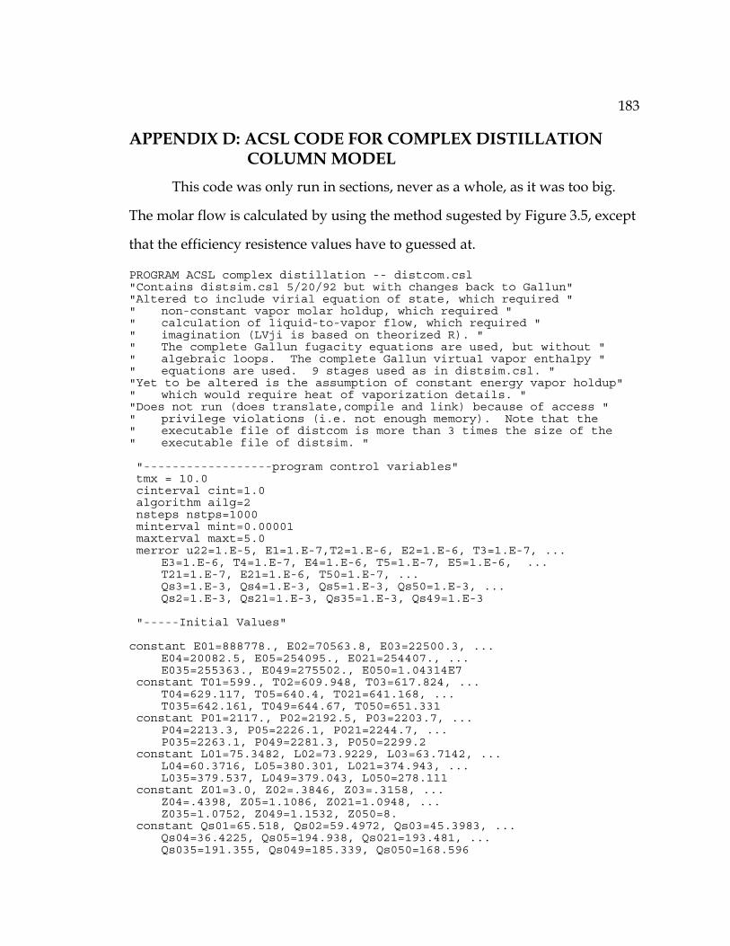
183

APPENDIX D: ACSL CODE FOR COMPLEX DISTILLATION COLUMN MODEL

This code was only run in sections, never as a whole, as it was too big.

The molar flow is calculated by using the method sugested by Figure 3.5, except

that the efficiency resistence values have to guessed at.

PROGRAM ACSL complex distillation -- distcom.csl "Contains distsim.csl 5/20/92 but with changes back to Gallun" "Altered to include virial equation of state, which required " " non-constant vapor molar holdup, which required " " calculation of liquid-to-vapor flow, which required " " imagination (LVji is based on theorized R). " " The complete Gallun fugacity equations are used, but without " " algebraic loops. The complete Gallun virtual vapor enthalpy " " equations are used. 9 stages used as in distsim.csl. " "Yet to be altered is the assumption of constant energy vapor holdup" " which would require heat of vaporization details. " "Does not run (does translate,compile and link) because of access " " privilege violations (i.e. not enough memory). Note that the " executable file of distcom is more than 3 times the size of the " executable file of distsim. " "------------------program control variables" tmx = 10.0 cinterval cint=1.0 algorithm ailg=2 nsteps nstps=1000 minterval mint=0.00001 maxterval maxt=5.0 merror u22=1.E-5, E1=1.E-7,T2=1.E-6, E2=1.E-6, T3=1.E-7, ... E3=1.E-6, T4=1.E-7, E4=1.E-6, T5=1.E-7, E5=1.E-6, ... T21=1.E-7, E21=1.E-6, T50=1.E-7, ... Qs3=1.E-3, Qs4=1.E-3, Qs5=1.E-3, Qs50=1.E-3, ... Qs2=1.E-3, Qs21=1.E-3, Qs35=1.E-3, Qs49=1.E-3 "-----Initial Values" constant E01=888778., E02=70563.8, E03=22500.3, ... E04=20082.5, E05=254095., E021=254407., ... E035=255363., E049=275502., E050=1.04314E7 constant T01=599., T02=609.948, T03=617.824, ... T04=629.117, T05=640.4, T021=641.168, ... T035=642.161, T049=644.67, T050=651.331 constant P01=2117., P02=2192.5, P03=2203.7, ... P04=2213.3, P05=2226.1, P021=2244.7, ... P035=2263.1, P049=2281.3, P050=2299.2 constant L01=75.3482, L02=73.9229, L03=63.7142, ... L04=60.3716, L05=380.301, L021=374.943, ... L035=379.537, L049=379.043, L050=278.111 constant Z01=3.0, Z02=.3846, Z03=.3158, ... Z04=.4398, Z05=1.1086, Z021=1.0948, ... Z035=1.0752, Z049=1.1532, Z050=8. constant Qs01=65.518, Qs02=59.4972, Qs03=45.3983, ... Qs04=36.4225, Qs05=194.938, Qs021=193.481, ... Qs035=191.355, Qs049=185.339, Qs050=168.596

184

constant how02=.0923, how03=.07707, how04=.06655, how05=.20362, ... how021=.2026, how035=.20111, how049=.19688, how050=.18483 constant u101=221.596, u201=126.272, u301=8.38675, u401=8.38675, ... u102=16.3432, u202=7.00848, u302=1.08277, u402=2.51991, ... u103=13.8607, u203=5.04879, u303=1.38213, u403=6.63553, ... u104=12.5007, u204=4.42564, u304=1.62497, u404=15.4035, ... u105=20.9044, u205=7.94464, u305=3.02323, u405=53.8308, ... u1021=20.8149, u2021=7.74166, u3021=3.04893, u4021=54.0149, ... u1035=20.4257, u2035=7.34855, u3035=3.09519, u4035=54.6731, ... u1049=20.0008, u2049=6.86185, u3049=3.28681, u4049=60.135, ... u1050=574.262, u2050=183.052, u3050=112.714, u4050=2527.614 constant uv101=1.30802, uv201=.75050, uv301=0.042886, ... uv401=0.042886, ... uv102=1.25504, uv202=0.71517, uv302=0.0475, ... uv402=0.0475, ... uv103=1.21071, uv203=0.56874, uv303=0.07024, uv403=0.14588, ... uv104=1.07025, uv204=0.46873, uv304=0.08298, uv404=0.34336, ... uv105=0.84613, uv205=0.38213, uv305=0.074752, uv405=0.58609, ... uv1021=0.85364, uv2021=0.37631, uv3021=0.07650, ... uv4021=.59697, ... uv1035=0.85569, uv2035=0.36361, uv3035=0.07933, ... uv4035=0.61844, ... uv1049=0.82964, uv2049=0.3333, uv3049=0.0835, ... uv4049=0.67621, ... uv1050=0.74581, uv2050=0.27694, uv3050=0.088916, ... uv4050=0.90691 constant V02=105.487, V03=104.062, V04=93.8535,V05=90.5108, ... V021=102.19, V035=101.833, V049=101.427, V050=102.23 constant LV101=0., LV201=0., LV301=0., LV401=0., ... LV102=.9683, LV202=6.8715, LV302=-1.23652, LV402=-5.17789, ... LV103=12.0247, LV203=7.2746, LV303=-0.30083, LV403=-8.7899, ... LV104=10.5706, LV204=4.0775, LV304=0.38116, LV404=-11.6866, ... LV105=-5.2853, LV205=-1.885, LV305=-0.52613, LV405=-3.9825, ... LV1021=0.3947, LV2021=0.8999, LV3021=-0.11441, LV4021=-0.823, ... LV1035=1.7418, LV2035=1.7496, LV3035=-.2031, LV4035=-2.8822, ... LV1049=6.6555, LV2049=3.796, LV3049=-0.06587, LV4049=-9.8906, ... LV1050=37.0355, LV2050=13.7452, LV3050=4.49227, LV4050=45.6589 constant I01=23.17856, I02=4.868, I03=7.26471, I04=26.7935, ... I05=31.3931, I06=11.142628, ... ZET01=.47433, ZET02=.510625, ZET03=.415932, ... ZET04=0.754757, ZET05=.726259 constant Tmc0=579.441, Two0=566.204, ... Tmr0=751.405, Tsc0=777.66, TM0=642.223 Rf = 30.0 "----------controller set-points, gains, time-constants" TABLE SP, 1, 6 /... 1,2,3,4,5,6, 760., 490.135, 3.0, 0.0, 8.0, 642.223/ CISP1 = 0.032*SP(1.0) - 12.0 CISP2 = (SP(2.0)/200)**2 + 4.0 CISP3 = 4.0 + 1.6*SP(3.0) CISP5 = -20.0 + 4*SP(5.0) CISP6 = 0.4*SP(6.0) - 232. " TABLE CISP, 1, 6 /... " " 1,2,3,4,5,6,... " " 12.32, 10.0058, 8.8, 0, 12.0, 24.889/" TABLE XKC,1,6/... 1,2,3,4,5,6,...

185

1.5, 0.25, 1.1, 0.15, 0.5, 0.5/ TABLE TAUI,1,6/... 1,2,3,4,5,6,... 3.0, 0.1, 0.75, 0.25, 1.0, 0.6/ TABLE TAUV,1,6/... 1,2,3,4,5,6,... 0.15, 0.15, 0.15, 0.2, 0.15, 0.15/ "--------coeficients " TABLE MV, 2, 3, 4 /... 1,2,3, 1,2,3,4,... 0.6451094E2, -0.1095359 , 0.1195526E-3,... 0.5686523E2, 0.468039E-2, 0.5094978E-4,... 0.5370027E2, -0.1728176E-1, 0.493820E-4,... 0.2288676E2, -0.2023121E-1, 0.2115899E-4/ TABLE HVCO, 2, 5, 4/... 1, 2, 3, 4, 5, 1, 2, 3, 4,... 0.1174119E5, 0.7121495E1, 0.5579442E-2, ... -0.450617E-6, -0.2091904E-10,... 0.867332E4, 0.4735799E1, 0.1452860E-1,... -0.1121397E-5, -0.2018173E-9,... 0.106486E5, 0.7515997E1, 0.1151360E-1,... -.01682096E-5, 0.9036333E-10,... 0.1545871E5, 0.8022526E1, -0.4745722E-3,... 0.6878047E-6, -0.1439752E-9/ TABLE hLCO, 2, 3, 4/... 1, 2, 3, 1, 2, 3, 4,... -0.3119436E4, -4.145198, 0.2131106E-1, ... -0.115334E5, 0.1770348E2, 0.1166435E-1, ... 0.4046348E3, -0.2410286E2, 0.472823E-1, ... -0.87838059E4, 0.175845E2, 0.3651369E-3/ TABLE ANT, 2, 3, 4/... 1,2,3, 1,2,3,4,... 7.87863, 1.47311E3, 2.3E2,... 7.02447, 1.16E3, 2.24E2,... 8.04494, 1.5543E3, 2.2265E2,... 7.96681, 1.66821E3,2.28E2/ TABLE WLMB,2,4,4/... 1,2,3,4, 1,2,3,4,... 0.0, 0.66408E3, 0.59844E3, 0.20530E3,... -0.21495E3, 0.0, 0.38170E2, 0.43964E3,... 0.51139E3, 0.41896E3, 0.0, 0.38230E3,... 0.48216E3, 0.140549E3, 0.95549E3, 0.0/ TABLE RHOSCO, 1, 5/... 1,2,3,4,5,... 1.031951E-2, 1.427797E1, 0.9414444, 2.048037, 5.956991/ TABLE hLSCO, 1, 5/... 1,2,3,4,5,... -1.6029E2, 8.06427E-2, 7.361453E-5, 1.501012E-6,... -9.9964334E-10/ TABLE HVSCO, 1, 5/... 1,2,3,4,5,... 5.448738E2, 8.039637E-1, 1.931794E-3, -3.938661E-6,... 1.907853E-9/ TABLE HEDCO, 2,4,2/... 1,2,3,4, 1,2,... 9.870927E1, -9.794161E-3, -1.95175E-6, -1.954559E-9,... 9.152028E1, -6.584299E-2, 7.533832E-5, -4.300139E-8/ TABLE CV1CO , 2, 5, 20/... 1,2,3,4,5,... 0.0,0.099,0.1,0.19,0.2,0.29,0.3,0.39,0.4,0.49,... 0.5,0.59,0.6,0.69,0.7,0.79,0.8,0.89,0.9,1.0,...

186

0.0, 0.0, 0.6759999E2, -0.6691973E3, 0.6691969E4,... 0.0, 0.0, 0.6759999E2, -0.6691973E3, 0.6691969E4,... 0.1, 0.676E1, 0.1345197E3, -0.1167920E4, 0.8667223E4,... 0.1, 0.676E1, 0.1345197E3, -0.1167920E4, 0.8667223E4,... 0.2, 0.5810001E2, 0.9598074E3, -7506973E4, 0.8598887E5,... 0.2, 0.5810001E2, 0.9598074E3, -7506973E4, 0.8598887E5,... 0.3, 0.165E3, .2038081E4, -0.768066E4, 0.8299831E5,... 0.3, 0.165E3, .2038081E4, -0.768066E4, 0.8299831E5,... 0.4, 0.375E3, 0.2991901E4, -0.6826715E4, 0.4807690E5,... 0.4, 0.375E3, 0.2991901E4, -0.6826715E4, 0.4807690E5,... 0.5, 0.654E3, 0.3068865E4, -0.5726895E4, 0.6382414E4,... 0.5, 0.654E3, 0.3068865E4, -0.5726895E4, 0.6382414E4,... 0.6, 0.91E3, 0.2114958E4, -0.2852868E5, 0.2237909E6,... 0.6, 0.91E3, 0.2114958E4, -0.2852868E5, 0.2237909E6,... 0.7, 0.106E4, 0.3122954E4, 0.1411841E5, -0.9347956E5,... 0.7, 0.106E4, 0.3122954E4, 0.1411841E5, -0.9347956E5,... 0.8, 0.142E4, 0.3142248E4, -0.2419347E5, 0.1177098E6,... 0.8, 0.142E4, 0.3142248E4, -0.2419347E5, 0.1177098E6,... 0.9, 0.161E4, 0.1834851E4, -0.6969128E3, 0.3484387E4,... 0.9, 0.161E4, 0.1834851E4, -0.6969128E3, 0.3484387E4/ TABLE CV2CO, 2, 5, 20/... 1,2,3,4,5,... 0.0,0.099,0.1,0.19,0.2,0.29,0.3,0.39,0.4,0.49,... 0.5,0.59,0.6,0.69,0.7,0.79,0.8,0.89,0.9,1.0,... 0.0, 0.0, 0.6759999E2, -0.6691973E3, 0.6691969E4,... 0.0, 0.0, 0.6759999E2, -0.6691973E3, 0.6691969E4,... 0.1, 0.676E1, 0.1345197E3, -0.1167920E4, 0.8667223E4,... 0.1, 0.676E1, 0.1345197E3, -0.1167920E4, 0.8667223E4,... 0.2, 0.172E2, 0.1609525E3, -0.5040024E3, 0.5344770E4,... 0.2, 0.172E2, 0.1609525E3, -0.5040024E3, 0.5344770E4,... 0.3, 0.3360001E2, 0.2204954E3, -0.1038741E4, 0.8337859E4,... 0.3, 0.3360001E2, 0.2204954E3, -0.1038741E4, 0.8337859E4,... 0.4, 0.5360001E2, 0.2628831E3, -0.9942312E3, 0.8153996E4,... 0.4, 0.5360001E2, 0.2628831E3, -0.9942312E3, 0.8153996E4,... 0.5, 0.7810001E2, 0.3086567E3, -0.1381982E4, 0.1085412E5,... 0.5, 0.7810001E2, 0.3086567E3, -0.1381982E4, 0.1085412E5,... 0.6, 0.106E3, 0.3578840E3, -0.1145935E4, 0.8670914E4,... 0.6, 0.106E3, 0.3578840E3, -0.1145935E4, 0.8670914E4,... 0.7, 0.139E3, 0.3888247E3, -0.1526535E4, 0.1038285E5,... 0.7, 0.139E3, 0.3888247E3, -0.1526535E4, 0.1038285E5,... 0.8, 0.173E3, 0.3950034E3, -0.6824436E3, 0.2324071E4,... 0.8, 0.173E3, 0.3950034E3, -0.6824436E3, 0.2324071E4,... 0.9, 0.208E3, 0.3282368E3, -0.1564725E4, 0.7823613E4,... 0.9, 0.208E3, 0.3282368E3, -0.1564725E4, 0.7823613E4/ TABLE CV3CO, 2, 5, 20/... 1,2,3,4,5,... 0.0,0.099,0.1,0.19,0.2,0.29,0.3,0.39,0.4,0.49,... 0.5,0.59,0.6,0.69,0.7,0.79,0.8,0.89,0.9,1.0,... 0.0, 0.0, 0.6689999E2, -0.17743E3, 0.1742997E4,... 0.0, 0.0, 0.6689999E2, -0.17743E3, 0.1742997E4,... 0.1, 0.669E1, 0.8432991E2, -0.8532524E3, 0.5009532E4,... 0.1, 0.669E1, 0.8432991E2, -0.8532524E3, 0.5009532E4,... 0.2, 0.116E2, 0.6396542E2, -0.3343521E3, 0.3846974E4,... 0.2, 0.116E2, 0.6396542E2, -0.3343521E3, 0.3846974E4,... 0.3, 0.185E2, 0.1125043E3, -0.6310693E3, 0.6060258E4,... 0.3, 0.185E2, 0.1125043E3, -0.6310693E3, 0.6060258E4,... 0.4, 0.295E2, 0.1680985E3, -0.9577654E3, 0.9167789E4,... 0.4, 0.295E2, 0.1680985E3, -0.9577654E3, 0.9167789E4,... 0.5, 0.4589999E2, 0.2515793E3, -0.132549E4, 0.1269696E5,... 0.5, 0.4589999E2, 0.2515793E3, -0.132549E4, 0.1269696E5,... 0.6, 0.705E2, 0.3673904E3, -0.1754303E4, 0.1630397E5,...

187

0.6, 0.705E2, 0.3673904E3, -0.1754303E4, 0.1630397E5,... 0.7, 0.106E3, 0.5056489E3, -0.2605563E4, 0.2349071E5,... 0.7, 0.106E3, 0.5056489E3, -0.2605563E4, 0.2349071E5,... 0.8, 0.154E3, 0.6892578E3, -0.2990246E4, 0.2697664E5,... 0.8, 0.154E3, 0.6892578E3, -0.2990246E4, 0.2697664E5,... 0.9, 0.22E3, 0.9005083E3, -0.1210117E4, 0.6050512E4,... 0.9, 0.22E3, 0.9005083E3, -0.1210117E4, 0.6050512E4/ TABLE CV5CO, 2, 5, 20/... 1,2,3,4,5,... 0.0,0.099,0.1,0.19,0.2,0.29,0.3,0.39,0.4,0.49,... 0.5,0.59,0.6,0.69,0.7,0.79,0.8,0.89,0.9,1.0,... 0.0, 0.0, 0.463E3, -0.3610995E4, 0.3610991E5,... 0.0, 0.0, 0.463E3, -0.3610995E4, 0.3610991E5,... 0.1, 0.463E2, 0.8240989E3, -0.5206883E4, 0.3035894E5,... 0.1, 0.463E2, 0.8240989E3, -0.5206883E4, 0.3035894E5,... 0.2, 0.107E3, 0.6934902E3, -0.1574331E4, 0.1039425E5,... 0.2, 0.107E3, 0.6934902E3, -0.1574331E4, 0.1039425E5,... 0.3, 0.171E3, 0.6904519E3, -0.2672921E4, 0.1468400E5,... 0.3, 0.171E3, 0.6904519E3, -0.2672921E4, 0.1468400E5,... 0.4, 0.228E3, 0.5963877E3, -0.2192055E4, 0.1328175E5,... 0.4, 0.228E3, 0.5963877E3, -0.2192055E4, 0.1328175E5,... 0.5, 0.279E3, 0.5564294E3, -0.1604116E4, 0.8398187E4,... 0.5, 0.279E3, 0.5564294E3, -0.1604116E4, 0.8398187E4,... 0.6, 0.327E3, 0.4875520E3, -0.1870622E4, 0.9950992E4,... 0.6, 0.327E3, 0.4875520E3, -0.1870622E4, 0.9950992E4,... 0.7, 0.367E3, 0.4119575E3, -0.4696677E3, -0.1499096E4,... 0.7, 0.367E3, 0.4119575E3, -0.4696677E3, -0.1499096E4,... 0.8, 0.402E3, 0.2730510E3, -0.1572119E4, 0.6416082E4,... 0.8, 0.402E3, 0.2730510E3, -0.1572119E4, 0.6416082E4,... 0.9, 0.42E3, 0.1511098E3, -0.4221873E3, 0.2110922E4,... 0.9, 0.42E3, 0.1511098E3, -0.4221873E3, 0.2110922E4/ TABLE CSCO , 2, 5, 20/... 1,2,3,4,5,... 0.0,0.099,0.1,0.19,0.2,0.29,0.3,0.39,0.4,0.49,... 0.5,0.59,0.6,0.69,0.7,0.79,0.8,0.89,0.9,1.0,... 0.0, 0.0, 0.112E3, -0.280999E3, 0.2809984,... 0.0, 0.0, 0.112E3, -0.280999E3, 0.2809984,... 0.1, 0.193E2, 0.9875446E2, -0.6029138E3, 0.6653684E4,... 0.1, 0.193E2, 0.9875446E2, -0.6029138E3, 0.6653684E4,... 0.2, 0.193E2, 0.9875446E2, -0.6029138E3, 0.6653684E4,... 0.2, 0.193E2, 0.9875446E2, -0.6029138E3, 0.6653684E4,... 0.3, 0.298E2, 0.1777826E3, -0.8587102E3, 0.8508832E4,... 0.3, 0.298E2, 0.1777826E3, -0.8587102E3, 0.8508832E4,... 0.4, 0.475E2, 0.2613057E3, -0.1764654E4, 0.1651596E5,... 0.4, 0.475E2, 0.2613057E3, -0.1764654E4, 0.1651596E5,... 0.5, 0.725E2, 0.4038538E3, -0.2260444E4, 0.2271903E5,... 0.5, 0.725E2, 0.4038538E3, -0.2260444E4, 0.2271903E5,... 0.6, 0.133E3, 0.6333362E3, -0.2353483E4, 0.2220118E5,... 0.6, 0.133E3, 0.6333362E3, -0.2353483E4, 0.2220118E5,... 0.7, 0.175E3, 0.8286753E3, -0.2622047E4, 0.1935291E5,... 0.7, 0.175E3, 0.8286753E3, -0.2622047E4, 0.1935291E5,... 0.8, 0.251E3, 0.8848535E3, -0.6906321E3, -0.4579047E4,... 0.8, 0.251E3, 0.8848535E3, -0.6906321E3, -0.4579047E4,... 0.9, 0.328E3, 0.6093555E3, -0.4187094E4, 0.2093548E5,... 0.9, 0.328E3, 0.6093555E3, -0.4187094E4, 0.2093548E5/ "--------Physical constants " TABLE PCC, 2, 4, 4/... 1,2,3,4, 1,2,3,4,... 78.5, 59.6, 70.0, 127.8,... 59.6, 46.6, 54.0, 93.5,... 70.0, 54.0, 63.0, 111.9,...

188

127.8, 93.5, 111.9, 218.3/ TABLE TCC, 2, 4, 4/... 1,2,3,4, 1,2,3,4,... 513.2, 510.9, 514.1, 576.4,... 510.9, 508.7, 512.3, 573.9,... 514.1, 512.3, 516.0, 578.0,... 576.4, 573.9, 578.0, 647.4/ TABLE TC,1,4/... 1,2,3,4,... 513.2, 508.7, 516.0, 647.4/ TABLE PC,1,4/... 1,2,3,4,... 78.5, 46.6, 63.0, 218.3/ TABLE VC,1,4/... 1,2,3,4,... 118.0, 213.5, 161.3, 55.2/ TABLE WW,1,4/... 1,2,3,4,... 0.557, 0.309, 0.637, 0.344/ TABLE WWH,1,4/... 1,2,3,4,... 0.105, 0.187, 0.152, 0.010/ TABLE MU,1,4/... 1,2,3,4,... 1.66, 2.88, 1.69, 1.83/ TABLE ETTA, 2,4,4/... 1,2,3,4, 1,2,3,4,... 1.21, 0.605, 1.155, 0.605,... 0.605, 0.0, 0.55, 0.0,... 1.155, 0.55, 1.1, 0.55,... 0.605, 0.0, 0.55, 0.0/ TABLE MUR, 2, 4, 4/... 1,2,3,4 ,1,2,3,4,... 4.408, 4.693, 4.308, 4.761,... 4.693, 5.006, 4.607, 5.008,... 4.308, 4.607, 4.213, 4.640,... 4.761, 5.008, 4.640, 5.161/ TABLE WH, 2, 4, 4/... 1,2,3,4, 1,2,3,4,... 0.105, 0.146, 0.1285, 0.0575,... 0.146, 0.187, 0.1695, 0.0985,... 0.1285, 0.1695, 0.152, 0.081,... 0.0575, 0.0985, 0.081, 0.01/ TABLE MOL, 1, 4/... 1,2,3,4,... 32.04,58.08,46.07,18.016/ "------------Column constants and forcing functions " TABLE AH, 1, 4/... 1,3,4,50,... 18,18,13,13/ TABLE CD, 1, 4/... 1, 3, 4, 50,... 0.75, 0.75, 0.72, 0.72/ TABLE F, 2, 10, 4/... 1,2,3,4,5,6,20,21,22,50,... 1,2,3,4,... 0., 0., 0., 0.,65.25, 0., 0., .0, 0., 0., ... 0., 0., 0., 0., 25.5, 0., 0., .0, 0., 0., ... 0., 0., 0., 0., 10.0, 0., 0., .0, 0., 0., ... 0., 0., 0., 0.,208.5, 0., 0., .0, 0., 0./ TABLE Hf, 1, 10/...

189

1,2,3,4,5,6,20,21,22,50,... 0.0, 0.0, 0.0, 0.0, 868000., 0.0, ... 0.0, 0.0, 0.0, 0.0/ "-----RECeiver liquid height to volume function" TABLE RECVOL, 1, 27/... 0.0,2.12692,5.99764,10.9848,16.8604,23.4904,42.8183,... 65.4004,90.6624,118.2,178.918,245.674,317.069,391.969,... 469.392,548.452,628.319,708.185,787.245,864.668,939.568,... 1010.96,1077.72,1138.44,1191.24,1233.15,1256.64,... 0.0,0.1,0.2,0.3,0.4,0.5,0.75,1.0,1.25,1.5,2.0,2.5,3.0,... 3.5,4.0,4.5,5.0,5.5,6.0,6.5,7.0,7.5,8.0,8.5,9.0,9.5,10.0/ TABLE LF, 2, 2,4/... 1,50, 1,2,3,4, ... 10.,10., 10., 10., 10.,10., 10.,10./ "-----Gas Constant in atm*ft**3/lBmol*K, cm**3*mmHg/gmol*K," " ft**3*mmHg/lBmol*R, cal/gmol*K, lb*ft**3/ft**2*lBmol*R" TABLE RR, 1, 5/... 1,2,3,4,5,... 1.314, 62361.0, 555.0, 1.987, 1545.0/ " Twi changed from 545." INITIAL Constant... pii=3.14159 , Twi=530. , Pw1=60 , Pw3=35 , PD=40 ,... PB=30 , TSH=960.0 , PSH=255.0 , HSH=1262.8 , TSAT=862.7 ,... AA=141.372 , AD=17.6715 , AN=141.372 , AT=176.714 ,... AUD=0.908375 , DH=0.1875, DTT=15.0 , HW=1.0 , HWSP=1.25 ,... LW=130.806 , LWSP=149.0 , TT=0.09375 , Apc=16022.16 ,... Aw=13940.0 , Ccw=1.0 , Cmc=0.12 , DR=10.0 , LR=16.0 ,... Pw2Pw3=9.0 , Qcwo=8653.0 , Ucw=17160.0 , Umc=45000.0 ,... Upmo=213.0 , Uwmo=1250.0 , Sv2IR=105.8752 , ZC=5.0 ,... ALPHA=0.2 , RHO2VR=0.002549852, As=3844.168 ,... Apmr=3361.826 , Cmr=0.12 , Us=1000.0 , Umr=11000.0,... Upmr=300.0 , Vr=68.83 , ZB=10.0 , ... TAUM=0.20 , P1P2R=27.09, REF1 = 0.947775644, REF2 = 9.0,... sumv1 = 1.0, g = 115523.24, Cx = .58, REF3=2.69413,... LH = 0.011208333, Cvc = .65 "gravitational acceleration, g, in ft/min**2" "------------------------Energy models-------------------------------" MACRO engder(dBmj, dB11, dB12, dB13, dB14, dB22, dB23, dB24, ... dB33, dB34, dB44,Yj1, Yj2, Yj3, Yj4,Tj, TKj) MACRO Redefine df311, df312, df313, df314, df322, df323, df324, ... df333, df334, df344, df411, df412, df413, df414, ... df422, df423, df424, df433, df434, df444, ... df511, df512, df513, df514, df522, df523, df524, ... df533, df534, df544, df611, df612, df613, df614, ... df622, df623, df624, df633, df634, df644 " The variables here are partial derivitives with respect to Tj" dBmj = (Yj1*Yj1*dB11 + Yj1*Yj2*dB12 ... + Yj1*Yj3*dB13 + Yj1*Yj4*dB14 ... + Yj2*Yj1*dB12 + Yj2*Yj2*dB22 ... + Yj2*Yj3*dB23 + Yj2*Yj4*dB24 ... + Yj3*Yj1*dB13 + Yj3*Yj2*dB23 ...

190

+ Yj3*Yj3*dB33 + Yj3*Yj4*dB34 ... + Yj4*Yj1*dB14 + Yj4*Yj2*dB24 ... + Yj4*Yj3*dB34 + Yj4*Yj4*dB44) dB11 = RR(1.0)*TCC(1.0,1.0)/PCC(1.0,1.0)*(df311 + WH(1.0,1.0)... *df411 + df511 + ETTA(1.0,1.0)*df611) dB12 = RR(1.0)*TCC(1.0,2.0)/PCC(1.0,2.0)*(df312 + WH(1.0,2.0)... *df412 + df512 + ETTA(1.0,2.0)*df612) dB13 = RR(1.0)*TCC(1.0,3.0)/PCC(1.0,3.0)*(df313 + WH(1.0,3.0)... *df413 + df513 + ETTA(1.0,3.0)*df613) dB14 = RR(1.0)*TCC(1.0,4.0)/PCC(1.0,4.0)*(df314 + WH(1.0,4.0)... *df414 + df514 + ETTA(1.0,4.0)*df614) dB22 = RR(1.0)*TCC(2.0,2.0)/PCC(2.0,2.0)*(df322 + WH(2.0,2.0)... *df422 + df522 + ETTA(2.0,2.0)*df622) dB23 = RR(1.0)*TCC(2.0,3.0)/PCC(2.0,3.0)*(df323 + WH(2.0,3.0)... *df423 + df523 + ETTA(2.0,3.0)*df623) dB24 = RR(1.0)*TCC(2.0,4.0)/PCC(2.0,4.0)*(df324 + WH(2.0,4.0)... *df424 + df524 + ETTA(2.0,4.0)*df624) dB33 = RR(1.0)*TCC(3.0,3.0)/PCC(3.0,3.0)*(df333 + WH(3.0,3.0)... *df433 + df533 + ETTA(3.0,3.0)*df633) dB34 = RR(1.0)*TCC(3.0,4.0)/PCC(3.0,4.0)*(df334 + WH(3.0,4.0)... *df434 + df534 + ETTA(3.0,4.0)*df634) dB44 = RR(1.0)*TCC(4.0,4.0)/PCC(4.0,4.0)*(df344 + WH(4.0,4.0)... *df444 + df544 + ETTA(4.0,4.0)*df644) df311 = -0.330*TCC(1.0,1.0)/TKj**2 + 0.1385*TCC(1.0,1.0)**2/TKj**3 ... + 0.0121*TCC(1.0,1.0)**3/TKj**4 df312 = -0.330*TCC(1.0,2.0)/TKj**2 + 0.1385*TCC(1.0,2.0)**2/TKj**3 ... + 0.0121*TCC(1.0,2.0)**3/TKj**4 df313 = -0.330*TCC(1.0,1.0)/TKj**2 + 0.1385*TCC(1.0,3.0)**2/TKj**3 ... + 0.0121*TCC(1.0,3.0)**3/TKj**4 df314 = -0.330*TCC(1.0,4.0)/TKj**2 + 0.1385*TCC(1.0,4.0)**2/TKj**3 ... + 0.0121*TCC(1.0,4.0)**3/TKj**4 df322 = -0.330*TCC(2.0,2.0)/TKj**2 + 0.1385*TCC(2.0,2.0)**2/TKj**3 ... + 0.0121*TCC(2.0,2.0)**3/TKj**4 df323 = -0.330*TCC(2.0,3.0)/TKj**2 + 0.1385*TCC(2.0,3.0)**2/TKj**3 ... + 0.0121*TCC(2.0,3.0)**3/TKj**4 df324 = -0.330*TCC(2.0,4.0)/TKj**2 + 0.1385*TCC(2.0,4.0)**2/TKj**3 ... + 0.0121*TCC(2.0,4.0)**3/TKj**4 df333 = -0.330*TCC(3.0,3.0)/TKj**2 + 0.1385*TCC(3.0,3.0)**2/TKj**3 ... + 0.0121*TCC(3.0,3.0)**3/TKj**4 df334 = -0.330*TCC(3.0,4.0)/TKj**2 + 0.1385*TCC(3.0,4.0)**2/TKj**3 ... + 0.0121*TCC(3.0,4.0)**3/TKj**4 df344 = -0.330*TCC(4.0,4.0)/TKj**2 + 0.1385*TCC(4.0,4.0)**2/TKj**3 ... + 0.0121*TCC(4.0,4.0)**3/TKj**4 df411 = - 0.4600*TCC(1.0,1.0)/TKj**2 ... + 0.5000*TCC(1.0,1.0)/TKj**3 ... + 0.0970*TCC(1.0,1.0)**3/TKj**4 ... + 0.0073*TCC(1.0,1.0)**8/TKj**9 df412 = - 0.4600*TCC(1.0,2.0)/TKj**2 ... + 0.5000*TCC(1.0,2.0)/TKj**3 ... + 0.0970*TCC(1.0,2.0)**3/TKj**4 ... + 0.0073*TCC(1.0,2.0)**8/TKj**9

191

df413 = - 0.4600*TCC(1.0,3.0)/TKj**2 ... + 0.5000*TCC(1.0,3.0)/TKj**3 ... + 0.0970*TCC(1.0,3.0)**3/TKj**4 ... + 0.0073*TCC(1.0,3.0)**8/TKj**9 df414 = - 0.4600*TCC(1.0,4.0)/TKj**2 ... + 0.5000*TCC(1.0,4.0)/TKj**3 ... + 0.0970*TCC(1.0,4.0)**3/TKj**4 ... + 0.0073*TCC(1.0,4.0)**8/TKj**9 df422 = - 0.4600*TCC(2.0,2.0)/TKj**2 ... + 0.5000*TCC(2.0,2.0)/TKj**3 ... + 0.0970*TCC(2.0,2.0)**3/TKj**4 ... + 0.0073*TCC(2.0,2.0)**8/TKj**9 df423 = - 0.4600*TCC(2.0,3.0)/TKj**2 ... + 0.5000*TCC(2.0,3.0)/TKj**3 ... + 0.0970*TCC(2.0,3.0)**3/TKj**4 ... + 0.0073*TCC(2.0,3.0)**8/TKj**9 df424 = - 0.4600*TCC(2.0,4.0)/TKj**2 ... + 0.5000*TCC(2.0,4.0)/TKj**3 ... + 0.0970*TCC(2.0,4.0)**3/TKj**4 ... + 0.0073*TCC(2.0,4.0)**8/TKj**9 df433 = - 0.4600*TCC(3.0,3.0)/TKj**2 ... + 0.5000*TCC(3.0,3.0)/TKj**3 ... + 0.0970*TCC(3.0,3.0)**3/TKj**4 ... + 0.0073*TCC(3.0,3.0)**8/TKj**9 df434 = - 0.4600*TCC(3.0,4.0)/TKj**2 ... + 0.5000*TCC(3.0,4.0)/TKj**3 ... + 0.0970*TCC(3.0,4.0)**3/TKj**4 ... + 0.0073*TCC(3.0,4.0)**8/TKj**9 df444 = - 0.4600*TCC(4.0,4.0)/TKj**2 ... + 0.5000*TCC(4.0,4.0)/TKj**3 ... + 0.0970*TCC(4.0,4.0)**3/TKj**4 ... + 0.0073*TCC(4.0,4.0)**8/TKj**9 df511 = (5.769770 - 6.181427*MUR(1.0,1.0) ... + 2.283270*MUR(1.0,1.0)**2 ... - 0.2649074*MUR(1.0,1.0)**3) *TCC(1.0,1.0)/TKj**2 df512 = (5.769770 - 6.181427*MUR(1.0,2.0) ... + 2.283270*MUR(1.0,2.0)**2 ... - 0.2649074*MUR(1.0,2.0)**3) *TCC(1.0,2.0)/TKj**2 df513 = (5.769770 - 6.181427*MUR(1.0,3.0) ... + 2.283270*MUR(1.0,3.0)**2 ... - 0.2649074*MUR(1.0,3.0)**3) *TCC(1.0,3.0)/TKj**2 df514 = (5.769770 - 6.181427*MUR(1.0,4.0) ... + 2.283270*MUR(1.0,4.0)**2 ... - 0.2649074*MUR(1.0,4.0)**3) *TCC(1.0,4.0)/TKj**2 df522 = (5.769770 - 6.181427*MUR(2.0,2.0) ... + 2.283270*MUR(2.0,2.0)**2 ... - 0.2649074*MUR(2.0,2.0)**3) *TCC(2.0,2.0)/TKj**2 df523 = (5.769770 - 6.181427*MUR(2.0,3.0) ... + 2.283270*MUR(2.0,3.0)**2 ... - 0.2649074*MUR(2.0,3.0)**3) *TCC(2.0,3.0)/TKj**2 df524 = (5.769770 - 6.181427*MUR(2.0,4.0) ... + 2.283270*MUR(2.0,4.0)**2 ... - 0.2649074*MUR(2.0,4.0)**3) *TCC(2.0,4.0)/TKj**2 df533 = (5.769770 - 6.181427*MUR(3.0,3.0) ... + 2.283270*MUR(3.0,3.0)**2 ... - 0.2649074*MUR(3.0,3.0)**3) *TCC(3.0,3.0)/TKj**2 df534 = (5.769770 - 6.181427*MUR(3.0,4.0) ... + 2.283270*MUR(3.0,4.0)**2 ... - 0.2649074*MUR(3.0,4.0)**3) *TCC(3.0,4.0)/TKj**2 df544 = (5.769770 - 6.181427*MUR(4.0,4.0) ... + 2.283270*MUR(4.0,4.0)**2 ...

192

- 0.2649074*MUR(4.0,4.0)**3) *TCC(4.0,4.0)/TKj**2 df611 = 101.49*EXP(-6.6*TKj/TCC(1.0,1.0)) df612 = 101.49*EXP(-6.6*TKj/TCC(1.0,2.0)) df613 = 101.49*EXP(-6.6*TKj/TCC(1.0,3.0)) df614 = 101.49*EXP(-6.6*TKj/TCC(1.0,4.0)) df622 = 101.49*EXP(-6.6*TKj/TCC(2.0,2.0)) df623 = 101.49*EXP(-6.6*TKj/TCC(2.0,3.0)) df624 = 101.49*EXP(-6.6*TKj/TCC(2.0,4.0)) df633 = 101.49*EXP(-6.6*TKj/TCC(3.0,3.0)) df634 = 101.49*EXP(-6.6*TKj/TCC(3.0,4.0)) df644 = 101.49*EXP(-6.6*TKj/TCC(4.0,4.0)) MACRO END MACRO engb1(Tj, TKj, R, QC, Ej, Lj, sumuj, EVjp, ... uj1, uj2, uj3, uj4, duj1,duj2,duj3,duj4, J) MACRO Redefine Ejdot, jj, dTj, hLj1, hLj2,hLj3,hLj4 jj = J/1.0 Ejdot = Hf(jj) + EVjp - (1 + R)*Lj*Ej/(R * sumuj) - QC Ej = INTEG(Ejdot, E0&J) hLj1 = hLCO(1.0,1.0) + hLCO(2.0,1.0)*Tj + hLCO(3.0,1.0)*Tj**2 hLj2 = hLCO(1.0,2.0) + hLCO(2.0,2.0)*Tj + hLCO(3.0,2.0)*Tj**2 hLj3 = hLCO(1.0,3.0) + hLCO(2.0,3.0)*Tj + hLCO(3.0,3.0)*Tj**2 hLj4 = hLCO(1.0,4.0) + hLCO(2.0,4.0)*Tj + hLCO(3.0,4.0)*Tj**2 Tj = INTEG(dTj, T0&J) TKj = 5.0*Tj/9.0 dTj = (Ejdot - hLj1*duj1 - hLj2*duj2 - hLj3*duj3 - hLj4*duj4)/ ... ((hLCO(2.0,1.0) + 2*hLCO(3.0,1.0)*Tj)*uj1 ... + (hLCO(2.0,2.0) + 2*hLCO(3.0,2.0)*Tj)*uj2 ... + (hLCO(2.0,3.0) + 2*hLCO(3.0,3.0)*Tj)*uj3 ... + (hLCO(2.0,4.0) + 2*hLCO(3.0,4.0)*Tj)*uj4) MACRO END MACRO engbj(Ej, Lj, Ljm, Ejm,uj1, uj2, uj3, uj4, ... sumuj, ujm1,ujm2,ujm3,ujm4,sumujm, ... duj1, duj2, duj3, duj4, Vj, EVj, EVjp, ... Yj1,Yj2,Yj3,Yj4, Tj, TKj, Bmj, Pj, ZZj, J) MACRO Redefine Ejdot,jj, dTj, OMEGAj, H01, H02,H03,H04, ... dBmj, dB11, dB12, dB13, dB14, dB22, dB23, dB24, ... dB33, dB34, dB44, hLj1,hLj2,hLj3,hLj4, ... HVj1, HVj2, HVj3,HVj4 engder(dBmj, dB11, dB12, dB13, dB14, dB22, dB23, dB24, ... dB33, dB34, dB44,Yj1, Yj2, Yj3, Yj4,Tj, TKj) jj = J/1.0 Ejdot = Hf(jj) + Ljm*Ejm/sumujm - Lj*Ej/sumuj - ... EVj + EVjp Ej = INTEG(Ejdot, E0&J) hLj1 = hLCO(1.0,1.0) + hLCO(2.0,1.0)*Tj + hLCO(3.0,1.0)*Tj**2 hLj2 = hLCO(1.0,2.0) + hLCO(2.0,2.0)*Tj + hLCO(3.0,2.0)*Tj**2 hLj3 = hLCO(1.0,3.0) + hLCO(2.0,3.0)*Tj + hLCO(3.0,3.0)*Tj**2 hLj4 = hLCO(1.0,4.0) + hLCO(2.0,4.0)*Tj + hLCO(3.0,4.0)*Tj**2 EVj = Vj*Yj1*HVj1 + Vj*Yj2*HVj2 + Vj*Yj3*HVj3 + ... Vj*Yj4*HVj4

193

HVj1 = H01 + OMEGAj HVj2 = H02 + OMEGAj HVj3 = H03 + OMEGAj HVj4 = H04 + OMEGAj H01 = HVCO(1.0,1.0) + HVCO(2.0,1.0)*Tj + HVCO(3.0,1.0)*Tj**2 + ... HVCO(4.0,1.0)*Tj**3 + HVCO(5.0,1.0)*Tj**4 H02 = HVCO(1.0,2.0) + HVCO(2.0,2.0)*Tj + HVCO(3.0,2.0)*Tj**2 + ... HVCO(4.0,2.0)*Tj**3 + HVCO(5.0,2.0)*Tj**4 H03 = HVCO(1.0,3.0) + HVCO(2.0,3.0)*Tj + HVCO(3.0,3.0)*Tj**2 + ... HVCO(4.0,3.0)*Tj**3 + HVCO(5.0,3.0)*Tj**4 H04 = HVCO(1.0,4.0) + HVCO(2.0,4.0)*Tj + HVCO(3.0,4.0)*Tj**2 + ... HVCO(4.0,4.0)*Tj**3 + HVCO(5.0,4.0)*Tj**4 OMEGAj = (2 - 1/ZZj)*Pj/(2*ZZj -1) * (TKj*dBmj - Bmj) Tj = INTEG(dTj, T0&J) TKj = 5.0*Tj/9.0 dTj = (Ejdot - hLj1*duj1 - hLj2*duj2 - hLj3*duj3 - hLj4*duj4)/ ... ((hLCO(2.0,1.0) + 2*hLCO(3.0,1.0)*Tj)*uj1 ... + (hLCO(2.0,2.0) + 2*hLCO(3.0,2.0)*Tj)*uj2 ... + (hLCO(2.0,3.0) + 2*hLCO(3.0,3.0)*Tj)*uj3 ... + (hLCO(2.0,4.0) + 2*hLCO(3.0,4.0)*Tj)*uj4) MACRO END MACRO engbN(Lj, Ljm, Ejm, QR,uj1, uj2, uj3, uj4, ... sumuj,ujm1, ujm2, ujm3, ujm4, sumujm, ... duj1, duj2, duj3, duj4, Vj, EVj, ... Yj1,Yj2,Yj3,Yj4, Tj, TKj, Bmj, Pj, ZZj, J) MACRO Redefine Ej, Ejdot, jj, dTj, H01,H02,H03,H04,... OMEGAj, dBmj,dB11,dB12,dB13,dB14,dB22,dB23,dB24, ... dB33, dB34, dB44, hLj1,hLj2,hLj3,hLj4, ... HVj1, HVj2, HVj3,HVj4 engder(dBmj, dB11, dB12, dB13, dB14, dB22, dB23, dB24, ... dB33, dB34,dB44,Yj1, Yj2, Yj3, Yj4,Tj, TKj) jj = J/1.0 Ejdot = Hf(jj) + Ljm*Ejm/sumujm - Lj*Ej/sumuj - EVj + QR Ej = INTEG(Ejdot, E0&J) hLj1 = hLCO(1.0,1.0) + hLCO(2.0,1.0)*Tj + hLCO(3.0,1.0)*Tj**2 hLj2 = hLCO(1.0,2.0) + hLCO(2.0,2.0)*Tj + hLCO(3.0,2.0)*Tj**2 hLj3 = hLCO(1.0,3.0) + hLCO(2.0,3.0)*Tj + hLCO(3.0,3.0)*Tj**2 hLj4 = hLCO(1.0,4.0) + hLCO(2.0,4.0)*Tj + hLCO(3.0,4.0)*Tj**2 EVj = Vj*Yj1*HVj1 + Vj*Yj2*HVj2 + Vj*Yj3*HVj3 + ... Vj*Yj4*HVj4 HVj1 = H01 + OMEGAj HVj2 = H02 + OMEGAj HVj3 = H03 + OMEGAj HVj4 = H04 + OMEGAj H01 = HVCO(1.0,1.0) + HVCO(2.0,1.0)*Tj + HVCO(3.0,1.0)*Tj**2 + ... HVCO(4.0,1.0)*Tj**3 + HVCO(5.0,1.0)*Tj**4 H02 = HVCO(1.0,2.0) + HVCO(2.0,2.0)*Tj + HVCO(3.0,2.0)*Tj**2 + ... HVCO(4.0,2.0)*Tj**3 + HVCO(5.0,2.0)*Tj**4 H03 = HVCO(1.0,3.0) + HVCO(2.0,3.0)*Tj + HVCO(3.0,3.0)*Tj**2 + ...

194

HVCO(4.0,3.0)*Tj**3 + HVCO(5.0,3.0)*Tj**4 H04 = HVCO(1.0,4.0) + HVCO(2.0,4.0)*Tj + HVCO(3.0,4.0)*Tj**2 + ... HVCO(4.0,4.0)*Tj**3 + HVCO(5.0,4.0)*Tj**4 OMEGAj = (2 - 1/ZZj)*Pj/(2*ZZj -1) * (TKj*dBmj - Bmj) Tj = INTEG(dTj, T0&J) TKj = 5.0*Tj/9.0 dTj = (Ejdot - hLj1*duj1 - hLj2*duj2 - hLj3*duj3 - hLj4*duj4)/ ... ((hLCO(2.0,1.0) + 2*hLCO(3.0,1.0)*Tj)*uj1 ... + (hLCO(2.0,2.0) + 2*hLCO(3.0,2.0)*Tj)*uj2 ... + (hLCO(2.0,3.0) + 2*hLCO(3.0,3.0)*Tj)*uj3 ... + (hLCO(2.0,4.0) + 2*hLCO(3.0,4.0)*Tj)*uj4) MACRO END "-----------------------Material-balance models--------------------" MACRO matb1(uj1, uj2, uj3, uj4, sumuj,duj1, duj2, duj3, duj4, ... Yjp1, Yjp2, Yjp3, Yjp4, Vjp, Suvj, LVj1,LVj2,LVj3,LVj4,... Yj1,Yj2,Yj3,Yj4, R, Lj, J) MACRO Redefine jj, uvj1, uvj2, uvj3, uvj4 jj = J/1.0 duj1 = f(jj,1.0) - (1 + R)*Lj*uj1/(R*sumu1) + Vjp*Yjp1 - LVj1 uj1 = INTEG(duj1, u10&J) duj2 = f(jj,2.0) - (1 + R)*Lj*uj2/(R*sumu1) + Vjp*Yjp2 - LVj2 uj2 = INTEG(duj2, u20&J) duj3 = f(jj,3.0) - (1 + R)*Lj*uj3/(R*sumu1) + Vjp*Yjp3 - LVj3 uj3 = INTEG(duj3, u30&J) duj4 = f(jj,4.0) - (1 + R)*Lj*uj4/(R*sumu1) + Vjp*Yjp4 - LVj4 uj4 = INTEG(duj4, u40&J) sumuj = uj1 + uj2 + uj3 + uj4 uvj1 = INTEG(LVj1, uv10&J) uvj2 = INTEG(LVj2, uv20&J) uvj3 = INTEG(LVj3, uv30&J) uvj4 = INTEG(LVj4, uv40&J) Suvj = uvj1 + uvj2 + uvj3 + uvj4 Yj1 = uvj1/Suvj Yj2 = uvj2/Suvj Yj3 = uvj3/Suvj Yj4 = uvj4/Suvj MACRO END MACRO matbj(uj1, uj2, uj3, uj4, sumuj,ujm1,ujm2, ujm3, ujm4, ... sumujm,duj1, duj2, duj3, duj4, Yj1,Yj2,Yj3,Yj4, Vj, ... Yjp1,Yjp2,Yjp3,Yjp4, Vjp, Lj, Ljm, ... LVj1,LVj2,LVj3,LVj4, Suvj, J) MACRO Redefine jj, duvj1,duvj2,duvj3,duvj4, ... uvj1,uvj2,uvj3,uvj4 jj = J/1.0 duj1 = f(jj,1.0) + Ljm*ujm1/sumujm - Lj*uj1/sumuj - LVj1 uj1 = INTEG(duj1, u10&J) duj2 = f(jj,2.0) + Ljm*ujm2/sumujm - Lj*uj2/sumuj - LVj2

195

uj2 = INTEG(duj2, u20&J) duj3 = f(jj,3.0) + Ljm*ujm3/sumujm - Lj*uj3/sumuj - LVj3 uj3 = INTEG(duj3, u30&J) duj4 = f(jj,4.0) + Ljm*ujm4/sumujm - Lj*uj4/sumuj - LVj4 uj4 = INTEG(duj4, u40&J) sumuj = uj1 + uj2 + uj3 + uj4 duvj1 = Vjp*Yjp1 - Vj*Yj1 + LVj1 uvj1 = INTEG(duvj1, uv10&J) duvj2 = Vjp*Yjp2 - Vj*Yj2 + LVj2 uvj2 = INTEG(duvj2, uv20&J) duvj3 = Vjp*Yjp3 - Vj*Yj3 + LVj3 uvj3 = INTEG(duvj3, uv30&J) duvj4 = Vjp*Yjp4 - Vj*Yj4 + LVj4 uvj4 = INTEG(duvj4, uv40&J) Suvj = uvj1 + uvj2 + uvj3 + uvj4 Yj1 = uvj1/Suvj Yj2 = uvj2/Suvj Yj3 = uvj3/Suvj Yj4 = uvj4/Suvj MACRO END MACRO matbN(uj1, uj2, uj3, uj4, sumuj,ujm1,ujm2, ujm3, ujm4, ... sumujm,duj1, duj2, duj3, duj4, Suvj, ... Vj, Vjp, Lj, Ljm, ... Yj1,Yj2,Yj3,Yj4, LVj1,LVj2,LVj3,LVj4, J) MACRO Redefine jj, duvj1, duvj2, duvj3, duvj4 jj = J*1.0/1.0 duj1 = f(jj,1.0) + Ljm*ujm1/sumujm - Lj*uj1/sumuj - LVj1 uj1 = INTEG(duj1, u10&J) duj2 = f(jj,2.0) + Ljm*ujm2/sumujm - Lj*uj2/sumuj - LVj2 uj2 = INTEG(duj2, u20&J) duj3 = f(jj,3.0) + Ljm*ujm3/sumujm - Lj*uj3/sumuj - LVj3 uj3 = INTEG(duj3, u30&J) duj4 = f(jj,4.0) + Ljm*ujm4/sumujm - Lj*uj4/sumuj - LVj4 uj4 = INTEG(duj4, u40&J) sumuj = uj1 + uj2 + uj3 + uj4 duvj1 = - Vj*uvj1/Suvj + LVj1 uvj1 = INTEG(duvj1, uv10&J) duvj2 = - Vj*uvj2/Suvj + LVj2 uvj2 = INTEG(duvj2, uv20&J) duvj3 = - Vj*uvj3/Suvj + LVj3 uvj3 = INTEG(duvj3, uv30&J) duvj4 = - Vj*uvj4/Suvj + LVj4 uvj4 = INTEG(duvj4, uv40&J) Suvj = uvj1 + uvj2 + uvj3 + uvj4 Yj1 = uvj1/Suvj Yj2 = uvj2/Suvj Yj3 = uvj3/Suvj Yj4 = uvj4/Suvj MACRO END "----------------------pressure models--------------------------"

196

MACRO pres1(Pj, Pjp, Z1, RHMLj, sumuj, Vjp, Tj, ZZj, Suvj, ... RHMVj, J) MACRO Redefine VOLREC, dP Pj = RR(5.0)*Tj*RHMVj*ZZj RHMVj = Suvj/(1256.6 - VOLREC) VOLREC = sumuj/RHMLj Z1 = RECVOL(VOLREC) dP = Pjp - Pj Vjp = SIGN(1.0,dP)*SQRT(ABS(dP)/(RHMVj*REF3)) MACRO END MACRO presj(Pj, Pjp, Lj, Ljm, HCTRj, HCTRjp, QQsj, ... RHOVj, RHMVj, RHMLj, RHOLj, RHOVjp, RHMVjp, ... sumuj, Vj, Vjp, Suvj, Yj1,Yj2,Yj3,Yj4, Tj, Zj, ZZj, ... LVj1,LVj2,LVj3,LVj4, Jp, J) MACRO Redefine HOj, FOAMj, QLj, FVAj, UVAj, UHj, HLUDj, ... MOLV, HOLDj, jj, dPdc, Pdc, dVdc, ... Vdc, dhow, howj, PUD, Qs, dQs, Cdd, dsumuj, dQVjp, ... dvjp, dZj, Pke jj = J/1.0 RHMVj = Suvj/(883.57 - sumuj/RHMLj) MOLV = Yj1*MOL(1.0) + Yj2*MOL(2.0) + Yj3*MOL(3.0) + ... Yj4*MOL(4.0) RHOVj = MOLV*RHMVj Pj = RR(5.0)*Tj*RHMVj*ZZj HCTRj = FOAMj*(howj + HW/12) FOAMj = 1 - 0.372192*FVAj**0.177709 FVAj = UVAj*SQRT(RHOVj) UVAj = Vjp/(AN*RHMVjp*60) " UHj = Vjp/(AH(jj)*RHMVjp)" " --HOj-- POj =(UHj/CD(jj))**2 * RHOVjp/(2*g)" Pke = RHOVjp*(Vjp/(AH(jj)*Cvc*RHMVjp))**2 /(2*g) dQVjp = Cvc**2*AH(jj)*(Pjp - Pj - HCTRj*RHOLj - Pke)/(RHOVj*LH) dVjp = dQVjp*RHMVj Vjp = INTEG(dVjp, V0&Jp) " ------downcomer hydrolic capacitance" " dPdc = RHOLj*dZj" " Pdc = INTEG(dPdc, (Zj*RHOLj))" dVdc = dZj * AD dZj = (Qs - QLj)/AD Vdc = Zj * AD Zj = INTEG(dZj,Z0&J) " --note that flows are allowed to become negative" QLj = Cx*AUD*SIGN(1.0,PUD)*SQRT(2*g*ABS(PUD)) PUD = (Pj - Pjp)/RHOLj - HCTRjp + Zj Lj = QLj*RHMLj " ------wier equations" dQs = Cdd*LW*dhow*SIGN(1.0,howj)*SQRT(2*g*ABS(howj))/12.0 QQsj = INTEG(dQs, Qs0&J ) Qs = FCNSW(howj, 0.0, 0.0, QQsj) Cdd = (1.368*(1.01 + .0063*(Qs*(12/LW)**2.5)))**1.5

197

dhow = (dsumuj/RHMLj - dVdc)/(AN*FOAMj) dsumuj = f(jj,1.0) + f(jj,2.0) + f(jj,3.0) + f(jj,4.0) + ... Ljm - Lj - (LVj1 + LVj2 + LVj3 + LVj4) howj = INTEG(dhow, how0&J ) MACRO END "-----------------------Liquid-Vapor equilibrium models----------" MACRO eqlcom(LMBjik, ALPHji, ALPHjk, Bjik,Tj, TKj, i, k) MACRO Redefine TRRjik, f3jik, f4jik, f5jik, f6jik LMBjik = ALPHjk/ALPHji * EXP(WLMB(i,k)/(RR(4.0)*TKj)) " TRRjik is reduced temperature here, as confirmed by" " [Perry, '73] , [°Kelvin/°Kelvin]" TRRjik = TKj/TCC(i,k) Bjik = RR(1.0)*TCC(i,k)*(f3jik + WH(i,k)*f4jik + f5jik + ... ETTA(i,k)*f6jik)/PCC(i,k) f3jik = 0.1445 - 0.330/TRRjik - 0.1385/(TRRjik**2) - ... 0.0121/(TRRjik**3) f4jik = 0.073 + 0.46/TRRjik - 0.5/(TRRjik**2) - 0.097/(TRRjik**3) ... - 0.0073/(TRRjik**8) f5jik = -5.237220 + 5.665807*MUR(i,k) - 2.133816*MUR(i,k)**2 + ... 0.2525373*MUR(i,k)**3 + (5.769770 - 6.181427*MUR(i,k) + ... 2.283270*MUR(i,k)**2 - 0.2649074*MUR(i,k)**3)/TRRjik f6jik = EXP(4.62 - 6.6*TRRjik) MACRO END MACRO eql(uj1, uj2, uj3, uj4, sumuj,Tj,TKj, ... Pj, Yj1, Yj2, Yj3, Yj4, RHMLj, RHOLj, ... ZZj, Bmj, RHMVj, ... LVj1,LVj2,LVj3,LVj4, J) MACRO Redefine PSj1, PSj2, PSj3, PSj4, Kj1, Kj2, Kj3 ,Kj4, ... ALPHj1, ALPHj2, ALPHj3, ALPHj4, ... PHIVj1, PHIVj2, PHIVj3, PHIVj4, ... GAMj1, GAMj2, GAMj3, GAMj4, ... PHILj1, PHISj1, f1j1, f2j1, TRj1, ... PHILj2, PHISj2, f1j2, f2j2, TRj2, ... PHILj3, PHISj3, f1j3, f2j3, TRj3, ... PHILj4, PHISj4, f1j4, f2j4, TRj4, ... Bj11, Bj12, Bj13, Bj14, Bj21, Bj22, Bj23, Bj24, Bj31, ... Bj32, Bj33, Bj34, Bj41, Bj42, Bj43, Bj44, ... LMBj11, LMBj12, LMBj13, LMBj14, LMBj21, LMBj22, ... LMBj23, LMBj24, LMBj31, LMBj32, LMBj33, LMBj34, ... LMBj41, LMBj42, LMBj43, LMBj44, jj, ... FgRj1, FgRj2, FgRj3, FgRj4, ... FgLj1,FgLj2,FgLj3,FgLj4, FgVj1,FgVj2,FgVj3,FgVj4, ... Rf1,Rf2,Rf3,Rf4, GAMs1,GAMs2,GAMs3,GAMs4 eqlcom(LMBj11, ALPHj1, ALPHj1, Bj11,Tj, TKj, 1.0, 1.0) eqlcom(LMBj12, ALPHj1, ALPHj2, Bj12,Tj, TKj, 1.0, 2.0) eqlcom(LMBj13, ALPHj1, ALPHj3, Bj13,Tj, TKj, 1.0, 3.0) eqlcom(LMBj14, ALPHj1, ALPHj4, Bj14,Tj, TKj, 1.0, 4.0) eqlcom(LMBj21, ALPHj2, ALPHj1, Bj21,Tj, TKj, 2.0, 1.0) eqlcom(LMBj22, ALPHj2, ALPHj2, Bj22,Tj, TKj, 2.0, 2.0) eqlcom(LMBj23, ALPHj2, ALPHj3, Bj23,Tj, TKj, 2.0, 3.0)

198

eqlcom(LMBj24, ALPHj2, ALPHj4, Bj24,Tj, TKj, 2.0, 4.0) eqlcom(LMBj31, ALPHj3, ALPHj1, Bj31,Tj, TKj, 3.0, 1.0) eqlcom(LMBj32, ALPHj3, ALPHj2, Bj32,Tj, TKj, 3.0, 2.0) eqlcom(LMBj33, ALPHj3, ALPHj3, Bj33,Tj, TKj, 3.0, 3.0) eqlcom(LMBj34, ALPHj3, ALPHj4, Bj34,Tj, TKj, 3.0, 4.0) eqlcom(LMBj41, ALPHj4, ALPHj1, Bj41,Tj, TKj, 4.0, 1.0) eqlcom(LMBj42, ALPHj4, ALPHj2, Bj42,Tj, TKj, 4.0, 2.0) eqlcom(LMBj43, ALPHj4, ALPHj3, Bj43,Tj, TKj, 4.0, 3.0) eqlcom(LMBj44, ALPHj4, ALPHj4, Bj44,Tj, TKj, 4.0, 4.0) jj = J/1.0 " ---liquid and vapor fugacity is calculated and then molar flow---" " The Rf values are guesses at this point" FgLj1 = GAMj1*uj1*PSj1*PHILj1/sumuj FgVj1 = PHIVj1*Yj1*Pj Rf1 = uvj1*Rf + 1. LVj1 = (FgLj1 - FgVj1)/Rf1 FgLj2 = GAMj2*uj2*PSj2*PHILj2/sumuj FgVj2 = PHIVj2*Yj2*Pj Rf2 = uvj2*Rf + 1. LVj2 = (FgLj2 - FgVj2)/Rf2 FgLj3 = GAMj3*uj3*PSj3*PHILj3/sumuj FgVj3 = PHIVj3*Yj3*Pj Rf3 = uvj3*Rf + 1. LVj3 = (FgLj3 - FgVj3)/Rf3 FgLj4 = GAMj4*uj4*PSj4*PHILj4/sumuj FgVj4 = PHIVj4*Yj4*Pj FgRj4 = LVj4*Rf4 Rf4 = uvj4*Rf + 1. LVj4 = (FgLj4 - FgVj4)/Rf4 "--------Liquid fugacity stuff-----------" PSj1 = 2.784605*10.**(ANT(1.0,1.0) - (ANT(2.0,1.0)/(ANT(3.0,1.0) + ... (TKj - 273.15)))) PSj2 = 2.784605*10.**(ANT(1.0,2.0) - (ANT(2.0,2.0)/(ANT(3.0,2.0) + ... (TKj - 273.15)))) PSj3 = 2.784605*10.**(ANT(1.0,3.0) - (ANT(2.0,3.0)/(ANT(3.0,3.0) + ... (TKj - 273.15)))) PSj4 = 2.784605*10.**(ANT(1.0,4.0) - (ANT(2.0,4.0)/(ANT(3.0,4.0) + ... (TKj - 273.15)))) GAMs1 = uj1*LMBj11 + uj1*LMBj12 + uj1*LMBj13 ... + uj1*LMBj14 GAMs2 = uj2*LMBj21 + uj2*LMBj22 + ... uj2*LMBj23 + uj2*LMBj24 GAMs3 = uj3*LMBj31 + uj3*LMBj32 + ... uj3*LMBj33 + uj3*LMBj34 GAMs4 = uj4*LMBj41 + uj4*LMBj42 + uj4*LMBj43 + ... uj4*LMBj44 GAMj1 = EXP(1 - uj1*LMBj11/GAMs1 - uj2*LMBj21/GAMs2 - ... uj3*LMBj31/GAMs3 - uj4*LMBj41/GAMs4) * ...

199

sumuj/(uj1*LMBj11 + uj2*LMBj12 + ... uj3*LMBj13 + uj4*LMBj14) GAMj2 = EXP(1 - uj1*LMBj12/GAMs1 - uj2*LMBj22/GAMs2 - ... uj3*LMBj32/GAMs3 - uj4*LMBj42/GAMs4) * ... sumuj/(uj1*LMBj21 + uj2*LMBj22 + uj3*LMBj23 + ... uj4*LMBj24) GAMj3 = EXP(1 - uj1*LMBj13/GAMs1 - uj2*LMBj23/GAMs2 - ... uj3*LMBj33/GAMs3 - uj4*LMBj43/GAMs4) * ... sumuj/(uj1*LMBj31 + uj2*LMBj32 + ... uj3*LMBj33 + uj4*LMBj34) GAMj4 = EXP(1 - uj1*LMBj14/GAMs1 - uj2*LMBj24/GAMs2 - ... uj3*LMBj34/GAMs3 - uj4*LMBj44/GAMs4) * ... sumuj/(uj1*LMBj41 + uj2*LMBj42 + ... uj3*LMBj43 + uj4*LMBj44) PHISj1 = EXP(f1j1 + f2j1*WW(1.0)) PHISj2 = EXP(f1j2 + f2j2*WW(2.0)) PHISj3 = EXP(f1j3 + f2j3*WW(3.0)) PHISj4 = EXP(f1j4 + f2j4*WW(4.0)) " Note that TRji is 9/5 of reduced temperature. " " Otherwise, PHILji <<1.0 for all Tj, which is improbable" " Hence, the dimension of TRji is [°Rankine/°Kelvin]" TRj1 = Tj/TC(1.0) TRj2 = Tj/TC(2.0) TRj3 = Tj/TC(3.0) TRj4 = Tj/TC(4.0) f1j1 = -3.5021358 + TRj1*( 5.6085595 + TRj1*(-3.076574 + ... TRj1*0.57335015)) f2j1 = -3.7690418 + TRj1*( 4.3538729 + TRj1*( 0.3166137 + ... TRj1*( ... 0.12666184 + TRj1*(-1.1662283 + TRj1*(-0.10665730 + TRj1*( ... 0.12147436 + TRj1*( 0.18927037 + TRj1*(0.14936906 + ... TRj1*(0.024364816 + TRj1*(-0.068603516 + TRj1*(-0.015172164 ... + TRj1*0.012089114))))))))))) f1j2 = -3.5021358 + TRj2*( 5.6085595 + TRj2*(-3.076574 + ... TRj2*0.57335015)) f2j2 = -3.7690418 + TRj2*( 4.3538729 + TRj2*( 0.3166137 + TRj2*(... 0.12666184 + TRj2*(-1.1662283 + TRj2*(-0.10665730 + TRj2*( ... 0.12147436 + TRj2*( 0.18927037 + TRj2*(0.14936906 + ... TRj2*(0.024364816 + TRj2*(-0.068603516 + TRj2*(-0.015172164 ... + TRj2*0.012089114))))))))))) f1j3 = -3.5021358 + TRj3*( 5.6085595 + TRj3*(-3.076574 + ... TRj3*0.57335015)) f2j3 = -3.7690418 + TRj3*( 4.3538729 + TRj3*( 0.3166137 + TRj3*(... 0.12666184 + TRj3*(-1.1662283 + TRj3*(-0.10665730 + TRj3*( ... 0.12147436 + TRj3*( 0.18927037 + TRj3*(0.14936906 + ... TRj3*(0.024364816 + TRj3*(-0.068603516 + TRj3*(-0.015172164 ... + TRj3*0.012089114))))))))))) f1j4 = -3.5021358 + TRj4*( 5.6085595 + TRj4*(-3.076574 + ... TRj4*0.57335015)) f2j4 = -3.7690418 + TRj4*( 4.3538729 + TRj4*( 0.3166137 + TRj4*(... 0.12666184 + TRj4*(-1.1662283 + TRj4*(-0.10665730 + TRj4*( ... 0.12147436 + TRj4*( 0.18927037 + TRj4*(0.14936906 + ...

200

TRj4*(0.024364816 + TRj4*(-0.068603516 + TRj4*(-0.015172164 ... + TRj4*0.012089114))))))))))) PHILj1 = PHISj1*EXP(ALPHj1*(- PSj1)/(2.784605*RR(2.0)*TKj)) PHILj2 = PHISj2*EXP(ALPHj2*(- PSj2)/(2.784605*RR(2.0)*TKj)) PHILj3 = PHISj3*EXP(ALPHj3*(- PSj3)/(2.784605*RR(2.0)*TKj)) PHILj4 = PHISj4*EXP(ALPHj4*(- PSj4)/(2.784605*RR(2.0)*TKj)) "-----Liquid densities----" ALPHj1 = MV(1.0,1.0) + MV(2.0,1.0)*Tj + MV(3.0,1.0)*Tj**2 ALPHj2 = MV(1.0,2.0) + MV(2.0,2.0)*Tj + MV(3.0,2.0)*Tj**2 ALPHj3 = MV(1.0,3.0) + MV(2.0,3.0)*Tj + MV(3.0,3.0)*Tj**2 ALPHj4 = MV(1.0,4.0) + MV(2.0,4.0)*Tj + MV(3.0,4.0)*Tj**2 RHMLj = 62.43*sumuj/(ALPHj1*uj1 +ALPHj2*uj2 + ... ALPHj3*uj3 + ALPHj4*uj4) RHOLj = 62.43*sumuj/(ALPHj1*uj1/MOL(1.0) + ... ALPHj2*uj2/MOL(2.0) + ... ALPHj3*uj3/MOL(3.0) + ... ALPHj4*uj4/MOL(4.0)) "---Vapor fugacity stuff----" PHIVj1 = EXP(2*(Yj1*Bj11 + Yj2*Bj12 + Yj3*Bj13 + Yj4*Bj14)* ... RHMVj) / ZZj PHIVj2 = EXP(2*(Yj1*Bj21+Yj2*Bj22 + Yj3*Bj23 + Yj4*Bj24)* ... RHMVj) / ZZj PHIVj3 = EXP(2*(Yj1*Bj31 + Yj2*Bj32 + Yj3*Bj33+Yj4*Bj34)* ... RHMVj) / ZZj PHIVj4 = EXP(2*(Yj1*Bj41 + Yj2*Bj42 + Yj3*Bj43+Yj4*Bj44)* ... RHMVj) / ZZj Bmj = (Yj1*(Yj1*Bj11 + Yj2*Bj12 + Yj3*Bj13 + Yj4*Bj14) + ... Yj2*(Yj1*Bj21 + Yj2*Bj22 + Yj3*Bj23 + Yj4*Bj24) + ... Yj3*(Yj1*Bj31 + Yj2*Bj32 + Yj3*Bj33 + Yj4*Bj34) + ... Yj4*(Yj1*Bj41 + Yj2*Bj42 + Yj3*Bj43 + Yj4*Bj44)) ZZj = 1.0 + Bmj*RHMVj MACRO END "-----------------------condenser and receiver model-------------" MACRO condsr(QC, L1, RHMLj, R, Pjp, Z1, Pj, q1, RHOL1, ... T1,T2, Vjp,CV1, CV2, CV3) MACRO Redefine Pd1, Ps1, q2, Qcw, Tmc, Two,... Z, Y, X, PDD Two = INTEG(((Qcw*Ccw*(Twi - Two)*8.34 + Uwmo/60 * Aw*(Tmc - ... Two)*(Qcw/Qcwo)**1.8 )/(Ucw*Ccw)), Two0) QC = (105.8752/(Vjp))**0.33 *(Upmo/60 * Apc*( ... (1-ALPHA)*T2 + ALPHA*T1 - Tmc)) Tmc = INTEG(((QC - Uwmo/60 * (Qcw/Qcwo)**1.8 * Aw*(Tmc - Two)) ... /(Umc*Cmc)), Tmc0) Qcw = ((Pw1 - Pw3)*CV1**2/(0.25 + ... REF2*CV1**2/Qcwo**1.8))**0.5157507757 "--recevier flow" R = q1/q2

201

L1 = q1*RHMLj/7.481 Pd1 = Pj + Ppmp + Ppe Ppmp = (HEDCO(1,1) + HEDCO(2,1)*(q1 + q2) + ... HEDCO(3,1)*(q1 + q2)**2 + HEDCO(4,1)*(q1 + q2)**3)*RHOL1 Ppe = (Z1 + ZC)*RHOL1 "hydraulic inductance = rho*volume/area is guessed at in the following" Pv1 = (q1/CV1)**2 / 144 q1 = INTEG((Pd1 + Pv1 - PD)/(RHOL1*100),q10) Pv2 = (q2/CV2)**2 / 144 q2 = INTEG((Pd1 + Pv2 - Pjp)(RHOL1*50),q20) MACRO END "-----------------------reboiler model--------------------------" MACRO reboil(HCTRj, QR, P50, Z50, L50, QQsj, Ljm, ... Wsh, RHOVj, RHMVj, RHMLj, RHOL50, RHMLjm, ... sumuj, Suvj,Yj1, Yj2, Yj3, Yj4, T50, CS4, CV5, ZZj) MACRO Redefine Tsc, Tmr, Ps2, Pd2, q50, RHOSC, hLSC, HVSC, ... VOLBTW, MOLV, HP, dHVSC, FVAj, Csc, dRHOSC, ... dhowj, howj, Qs, dQs, Cdd "-----------pressure---" RHMVj = Suvj/(2297.290 - Z50*176.7146) MOLV = Yj1*MOL(1.0) + Yj2*MOL(2.0) + Yj3*MOL(3.0) + ... Yj4*MOL(4.0) RHOVj = MOLV*RHMVj VOLBTW = 100 + pii*Z50*DTT**2/4 HCTRj = howj + 1.25/12 dhowj = (Ljm/RHMLjm - Qs)/11.01 howj = INTEG(dhowj, how050 ) dQs = Cdd*149.0*dhowj*SIGN(1.0,howj)*SQRT(2*g*ABS(howj))/12.0 QQsj = INTEG(dQs, Qs050 ) Qs = FCNSW(howj, 0.0, 0.0, QQsj) Cdd = (1.368*(1.01 + .0063*(Qs*(12/LW)**2.5)))**1.5 Z50 = 4/(pii*DTT**2)*(sumuj/RHMLj - 100) P50 = RR(5.0)*T50*RHMVj*ZZj "--------------reboiler enthalpy balance and pump presures---" Tmr = INTEG(((Us*As/60 * (Tsc - Tmr) - QR)/(Umr*Cmr)), ... Tmr0) Tsc = INTEG(((Wsh*(HSH - hLSC) - Us*As/60 * (Tsc - Tmr)) ... /(Csc*Vr*RHOSC - hLSC*dRHOSC*Vr)), Tsc0) Csc = dHVSC + HVSC*dRHOSC/RHOSC QR = Upmr*Apmr/60 * (Tmr - T50) q50 = (0.0156369 + SQRT((0.0156369)**2 - 4*(-2.7865E-5 - ... 144/(62.4*CV5**2)) * (70.3698 - HP)))/(2* ... (-2.7865E-5 - 144/(62.4*CV5**2)) ) HP = PB*144/RHOL50 - Ps2 L50 = q50*RHMLj/7.481 Wsh = 2*PSH*CS4/(60*(1.0 + 0.00065*(TSH - TSAT))) RHOSC = 1.031951E-2 + 1.427797E1*Tsc/610 + 0.9414444* ... (Tsc/610)**2 ... + 2.048037*(Tsc/610)**3 + 5.956991*(Tsc/610)**4 dRHOSC = ( RHOSCO(2.0) + 2*RHOSCO(3.0)*Tsc/610 + 3*RHOSCO(4.0)...

202

*(Tsc/610)**2 + 4*RHOSCO(5.0)*(Tsc/610)**3 )/610 hLSC = -1.6029E2 + 8.06427E-2*Tsc + 7.361453E-5*Tsc**2 + ... 1.501012E-6*Tsc**3 - 9.9964334E-10*Tsc**4 dHVSC = 8.039637E-1 + 2*1.931794E-3*Tsc - 3*3.938661E-6* ... Tsc**2 + 4*1.907853E-9 * Tsc**3 HVSC = 5.448738E2 + 8.039637E-1*Tsc + 1.931794E-3*Tsc**2 - ... 3.938661E-6*Tsc**3 + 1.907853E-9*Tsc**4 Ps2 = P50/RHOL50 + Z50 + ZB MACRO END "----------------------Controllers model------------------------" MACRO contrl(CV1, CV2, CV3, CS4, CV5, ... T35, TK35, Pj, q1, Z1, Z50, Wsh) MACRO Redefine CI1, CI2, CI3, CI4, CI5, CI6, CO1, CO2, CO3, ... CO4, CO5, CO6, I1, I2, I3, I4, I5, I6, TM, ZETA1, ZETA2, ... ZETA3, ZETA4, ZETA5, dZETA1, dZETA2, dZETA3, dZETA5 CV1 = CV1CO(2.0,ZETA1) + CV1CO(3.0,ZETA1)*( ZETA1 ... - CV1CO(1.0,ZETA1)) + CV1CO(4.0,ZETA1)*( ZETA1 ... - CV1CO(1.0,ZETA1))**2 ... + CV1CO(5.0,ZETA1)*(ZETA1 - CV1CO(1.0,ZETA1))**3 CV2 = CV2CO(2.0,ZETA2) + CV2CO(3.0,ZETA2)*( ZETA2 ... - CV2CO(1.0,ZETA2)) + CV2CO(4.0,ZETA2)*( ZETA2 ... - CV2CO(1.0,ZETA2))**2 ... + CV2CO(5.0,ZETA2)*(ZETA2 - CV2CO(1.0,ZETA2))**3 CV3 = CV3CO(2.0,ZETA3) + CV3CO(3.0,ZETA3)*( ZETA3 ... - CV3CO(1.0,ZETA3)) + CV3CO(4.0,ZETA3)*( ZETA3 ... - CV3CO(1.0,ZETA3))**2 ... + CV3CO(5.0,ZETA3)*(ZETA3 - CV3CO(1.0,ZETA3))**3 CS4 = CSCO(2.0,ZETA4) + CSCO(3.0,ZETA4)*(ZETA4 ... - CSCO(1.0,ZETA4)) + CSCO(4.0,ZETA4)*(ZETA4 ... - CSCO(1.0,ZETA4))**2 + CSCO(5.0,ZETA4)*(ZETA4 ... - CSCO(1.0,ZETA4))**3 CV5 = CV5CO(2.0,ZETA5) + CV5CO(3.0,ZETA5)*(ZETA5 ... - CV5CO(1.0,ZETA5)) + CV5CO(4.0,ZETA5)*(ZETA5 ... - CV5CO(1.0,ZETA5))**2 + CV5CO(5.0,ZETA5)*(ZETA5 ... - CV5CO(1.0,ZETA5))**3 Pbob = Pj/2.784605 CI1 = 0.032*Pbob - 12.0 I1 = INTEG((CI1 - CISP1), I01) CO1 = XKC(1.0)*(CI1 - CISP1 + I1/TAUI(1.0)) ZETA1 = INTEG(dZETA1, ZET01) dZETA1 = (-0.25 + 0.0625*CO1 - ZETA1)/TAUV(1.0) CI2 = (q1/200)**2 + 4.0 I2 = INTEG(CISP2 - CI2, I02) CO2 = XKC(2.0)*(-CI2 + CISP2 + I2/TAUI(2.0)) ZETA2 = INTEG( dZETA2, ZET02) dZETA2 = (-0.25 + 0.0625*CO2 - ZETA2)/TAUV(2.0) CI3 = 4.0 + 1.6*Z1 I3 = INTEG(CI3 - CISP3, I03) CO3 = XKC(3.0)*(CI3 - CISP3 + I3/TAUI(3.0)) ZETA3 = INTEG(dZETA3, ZET03) dZETA3 = (-0.25 + 0.0625*CO3 - ZETA3)/TAUV(3.0) CI5 = -20.0 + 4*Z50

203

I5 = INTEG(CI5 - CISP5, I05) CO5 = XKC(5.0)*(CI5 - CISP5 + I5/TAUI(5.0)) ZETA5 = INTEG(dZETA5, ZET05) dZETA5 = (-0.25 + 0.0625*CO5 - ZETA5)/TAUV(5.0) CI4 = 4 + 16*(Wsh/3000)**2 I4 = INTEG(CO6 - CI4, I04) CO4 = XKC(4.0)*(CO6 - CI4 + I4/TAUI(4.0)) ZETA4 = INTEG((-0.25 + 0.0625*CO4 - ZETA4)/TAUV(4.0), ... ZET04) TM = INTEG((T35 - TM)/TAUM , TM0) CI6 = 0.4*TM - 232. CO6 = XKC(6.0)*(CISP6 - CI6 + I6/TAUI(6.0)) I6 = INTEG(CISP6 - CI6, I06) MACRO END "-----------------------------------stage 1 model------------------" MACRO cond(Tj,Tjp, Vjp, uj1, uj2, uj3, uj4, sumuj,... Yjp1,Yjp2,Yjp3,Yjp4, CV1, CV2, CV3, EVjp, ... RHOLj, RHMLjp, RHOVjp, RHMVjp, ... Pj, Pjp, HCTRjp, Lj, Ej, q1, Zj) MACRO Redefine R, QC, TKj, RHMLj, Yj1,Yj2,Yj3,Yj4, ... duj1,duj2,duj3,duj4, Suvj, LVj1, LVj2, LVj3,LVj4, ... ZZj, Bmj, RHMVj engb1(Tj, TKj, R, QC, Ej, Lj, sumuj, EVjp,... uj1, uj2, uj3, uj4, duj1,duj2,duj3,duj4, 1) matb1(uj1, uj2, uj3, uj4, sumuj,duj1, duj2, duj3, duj4, ... Yjp1, Yjp2, Yjp3, Yjp4, Vjp, Suvj,LVj1,LVj2,LVj3,LVj4, ... Yj1,Yj2,Yj3,Yj4, R, Lj, 1) eql(uj1, uj2, uj3, uj4, sumuj,Tj,TKj, ... Pj, Yj1, Yj2, Yj3, Yj4, RHMLj, RHOLj, ... ZZj, Bmj, RHMVj , ... LVj1,LVj2,LVj3,LVj4, 1) pres1(Pj, Pjp, Zj, RHMLj, sumuj, Vjp, Tj, ZZj, Suvj, ... RHMVj, 1) condsr(QC, Lj, RHMLj, R, Pjp, Zj, Pj, q1, RHOLj, ... Tj,Tjp, Vjp,CV1, CV2, CV3) MACRO END "-----------------------------------stage 2-49 model--------------" MACRO stage(uj1, uj2, uj3, uj4, sumuj,ujm1, ujm2, ujm3, ujm4, ... sumujm, Tj,TKj, Vj,Vjp, Yjp1,Yjp2,Yjp3,Yjp4, ... Yj1,Yj2,Yj3,Yj4, EVj, EVjp, Qsj, ... RHOLj, RHOVj, RHMVj, RHMLj, RHOVjp, RHMVjp, ... Zj, Pjp, HCTRjp,Pj, HCTRj,Ljm, Ejm,Lj, Ej, Jp, J) MACRO Redefine duj1, duj2, duj3, duj4, ... LVj1,LVj2,LVj3,LVj4, Bmj, ZZj, Suvj eql(uj1, uj2, uj3, uj4, sumuj,Tj,TKj, ... Pj, Yj1, Yj2, Yj3, Yj4, RHMLj, RHOLj, ... ZZj, Bmj, RHMVj, ... LVj1,LVj2,LVj3,LVj4, J) matbj(uj1, uj2, uj3, uj4, sumuj,ujm1,ujm2, ujm3, ujm4, ... sumujm,duj1, duj2, duj3, duj4, Yj1,Yj2,Yj3,Yj4, Vj, ... Yjp1,Yjp2,Yjp3,Yjp4, Vjp, Lj, Ljm, ... LVj1,LVj2,LVj3,LVj4, Suvj, J) engbj(Ej, Lj, Ljm, Ejm,uj1, uj2, uj3, uj4, ...

204

sumuj,ujm1, ujm2, ujm3, ujm4, sumujm, ... duj1, duj2, duj3, duj4, Vj, EVj, EVjp, ... Yj1,Yj2,Yj3,Yj4, Tj, TKj, Bmj, Pj, ZZj, J) presj(Pj, Pjp, Lj, Ljm, HCTRj, HCTRjp, Qsj, ... RHOVj, RHMVj, RHMLj, RHOLj, RHOVjp, RHMVjp, ... sumuj, Vj, Vjp, Suvj, Yj1,Yj2,Yj3,Yj4, Tj, Zj,ZZj, ... LVj1,LVj2,LVj3,LVj4, Jp,J) MACRO END "-----------------------------------stage 50 model----------------" MACRO rebo(uj1, uj2, uj3, uj4, sumuj,ujm1, ujm2, ujm3, ujm4, ... sumujm, Vj, Yj1, Yj2, Yj3, Yj4, ... RHOLj, RHOVj, RHMVj, EVj, Pj, Qsj, ... HCTRj,Ljm, Ejm,CS4, CV5, Zj, Wsh, Lj, Tj, J) MACRO Redefine QR, RHMLj, TKj, FgLj1,FgLj2,FgLj3,FgLj4, ... Suvj, Bmj, ZZj, LVj1,LVj2,LVj3,LVj4 engbN(Lj, Ljm, Ejm, QR,uj1, uj2, uj3, uj4, ... sumuj,ujm1, ujm2, ujm3, ujm4, sumujm, ... duj1, duj2, duj3, duj4, Vj, EVj, ... Yj1,Yj2,Yj3,Yj4, Tj, TKj, Bmj, Pj, ZZj, J) matbN(uj1, uj2, uj3, uj4, sumuj,ujm1,ujm2, ujm3, ujm4, ... sumujm,duj1, duj2, duj3, duj4, Suvj, ... Vj, Vjp, Lj, Ljm, ... Yj1,Yj2,Yj3,Yj4, LVj1,LVj2,LVj3,LVj4, J) eql(uj1, uj2, uj3, uj4, sumuj,Tj,TKj, ... Pj, Yj1, Yj2, Yj3, Yj4, RHMLj, RHOLj, ... ZZj, Bmj, RHMVj, ... LVj1,LVj2,LVj3,LVj4, J) reboil(HCTRj, QR, Pj, Zj, Lj, Qsj, Ljm, ... Wsh, RHOVj, RHMVj, RHMLj, RHOLj, RHMLj, ... sumuj, Suvj,Yj1, Yj2, Yj3, Yj4, Tj, CS4, CV5, ZZj) MACRO END END $" of INITIAL" "-----------------------------------------------------------------" DYNAMIC DERIVATIVE cond(T1,T2, V2, u11, u12, u13, u14, sumu1,... Y21,Y22,Y23,Y24, CV1, CV2, CV3, EV2, ... RHOL1, RHML2, RHOV2, RHMV2, ... P1, P2, HCTR2, L1, E1, q1, Z1) stage(u21, u22, u23, u24, sumu2,u11, u12, u13, u14, ... sumu1, T2,TK2, V2,V3, Y31,Y32,Y33,Y34, ... Y21,Y22,Y23,Y24, EV2, EV3, Qs2, ... RHOL2, RHOV2, RHMV2, RHML2, RHOV3, RHMV3, ... Z2, P3, HCTR3,P2, HCTR2,L1, E1,L2, E2, 3,2) stage(u31, u32, u33, u34, sumu3,u21, u22, u23, u24, ... sumu2, T3,TK3, V3,V4, Y41,Y42,Y43,Y44, ... Y31,Y32,Y33,Y34, EV3, EV4, Qs3, ... RHOL3, RHOV3, RHMV3, RHML3, RHOV4, RHMV4, ... Z3, P4, HCTR4,P3, HCTR3,L2, E2,L3, E3, 4,3) stage(u41, u42, u43, u44, sumu4,u31, u32, u33, u34, ... sumu3, T4,TK4, V4,V5, Y51,Y52,Y53,Y54, ... Y41,Y42,Y43,Y44, EV4, EV5, Qs4,... RHOL4, RHOV4, RHMV4, RHML4, RHOV5, RHMV5, ... Z4, P5, HCTR5,P4, HCTR4,L3, E3,L4, E4, 5,4) stage(u51, u52, u53, u54, sumu5,u41, u42, u43, u44, ...

205

sumu4, T5,TK5, V5,V21, Y211,Y212,Y213,Y214, ... Y51,Y52,Y53,Y54, EV5, EV21, Qs5,... RHOL5, RHOV5, RHMV5, RHML5, RHOV21, RHMV21, ... Z5, P21, HCTR21,P5, HCTR5,L4, E4,L5, E5, 21,5) stage(u211, u212, u213, u214, sumu21,u51, u52, u53, u54, ... sumu5, T21,TK21, V21,V35, Y351,Y352,Y353,Y354, ... Y211,Y212,Y213,Y214, EV21, EV35, Qs21,... RHOL21, RHOV21, RHMV21, RHML21, RHOV35, RHMV35, ... Z21, P35, HCTR35,P21, HCTR21,L5, E5,L21, E21, 35,21) stage(u351,u352,u353,u354, sumu35,u211,u212,u213,u214, ... sumu21, T35,TK35, V35,V49, Y491,Y492,Y493,Y494, ... Y351,Y352,Y353,Y354, EV35, EV49, Qs35,... RHOL35, RHOV35, RHMV35, RHML35, RHOV49, RHMV49, ... Z35, P49, HCTR49,P35, HCTR35,L21, E21,L35, E35, 49,35) stage(u491,u492,u493,u494, sumu49,u351,u352,u353,u354, ... sumu35, T49,TK49, V49,V50, Y501,Y502,Y503,Y504, ... Y491,Y492,Y493,Y494, EV49, EV50, Qs49,... RHOL49, RHOV49, RHMV49, RHML49, RHOV50, RHMV50, ... Z49, P50, HCTR50,P49, HCTR49,L35, E35,L49, E49, 50,49) rebo(u501,u502,u503,u504, sumu50, u491,u492,u493, u494, ... sumu49, V50, Y501, Y502, Y503, Y504, ... RHOL50, RHOV50, RHMV50, EV50, P50, Qs50, ... HCTR50,L49, E49,CS4, CV5, Z50, Wsh, L50, T50, 50) contrl(CV1, CV2, CV3, CS4, CV5, ... T35, TK35, P1, q1, Z1, Z50, Wsh) END $ "of DERIVATIVE" Termt(t .ge.tmx) END $ "of DYNAMIC" END $"of Program distcom.csl"

206

REFERENCES

[1] M. Van Winkle, Distillation, New York: McGraw-Hill Book Co., 1967.

[2] M. J. Lockett, Distillation Tray Fundamentals, Cambridge: Cambridge University Press, 1986.

[3] R. J. P. Brierley, “Developments in Distillation Equipment and System Design—Implications for Dynamics and Control,” Dynamics and Control of Chemical Reactors and Distillation Columns (IFAC Proceedings series; 4), pp. 25-30, 1988.

[4] C. D. Holland, Fundamentals of Multicomponent Distillation, New York: McGraw-Hill Book Co., 1981.

[5] F. E. Cellier, Continuous Systems Modeling, Springer-Verlag: New York. 1991.

[6] M. Amrhein, Modeling of Chemical Reaction Networks Using Bond Graphs, report for the Dept. of Electrical Engineering, University of Arizona, Tucson, 1990.

[7] P. C. Breedveld, “Multibond Graph Elements in Physical Systems Theory,” Journal of The Franklin Institute, vol. 319, no. 1/2, pp. 1-36, January/February 1985.

[8] J. Montbrun-DiFilippo, M. Delgado, C. Brie, and H. M. Paynter, “A Survey of Bond Graphs: Theory, Applications and Programs,” Journal of The Franklin Institute, vol. 328, no. 5/6, pp. 565-606, 1991.

[9] P. C. Breedveld, “Thermodynamic Bond Graphs: a New Synthesis,” International Journal of Modelling & Simulation, vol. 1, no. 1, pp. 57-61, 1981.

[10] P. C. Breedveld, “A Thermodynamic Framework for Physical Systems Theory,” Simulation and Model-based Methodologies: an Integrative View, NATO ASI Series F #10, Berlin: Springer-Verlag, pp. 603-606, 1984.

[11] P. C. Breedveld, “Thermodynamic Bond Graphs and the Problem of Thermal Inertance,” Journal of The Franklin Institute, vol. 314, no. 1, pp. 15-40, July 1982.

207

[12] G. F. Oster and C. A. Desoer, “Tellegen’s Theorem and Thermodynamic Inequalities,” Journal of Theoretical Biology, vol. 32, no. 2, pp. 219-241, August 1971.

[13] J. J. van Dixhoorn, “Physical Modelling on a Thermodynamic Basic Using the Bond Graph Concept,” Proceedings of the 10th IMACS World Congress on System Simulation and Scientific Computation, (Montreal), vol. 3, pp. 386-391, August 1982.

[14] R. S. H. Mah, S. Michaelson, and R. W. H. Sargent, “Dynamic Behavior of Multi-component Multi-stage Systems. Numerical Methods for the Solution,” Chemical Engineering Science, vol. 17, pp. 619-639, August 1962.

[15] E. L. Meadows, “Multicomponent Batch-distillation Calculations on a Digital Computer,” Chemical Engineering Progress Symposium Series #46: Process Systems Engineering, vol. 59, pp. 48-55, 1963.

[16] G. P. Distefano, “Mathematical Modeling and Numerical Integration of Multicomponent Batch Distillation Equations,” AIChE Journal, vol. 14, no. 1, pp. 190-199, January 1968.

[17] K. Alejski, “Computation of the Reacting Distillation Column Using a Liquid Mixing Model on the Plates,” Computers & Chemical Engineering, vol. 15, no. 5, pp. 313-323, May 1991.

[18] W. K. Chan, J. F. Boston, and L. B. Evans, “Select the Right Software for Modeling Separation Process,” Chemical Engineering Progress, vol. 87, no. 9, pp. 63-69, September 1991.

[19] R. E. Levy, A. S. Foss, and E. A. Grens II, “Response Modes of a Binary Distillation Column,” Industrial & Engineering Chemistry Fundamentals, vol. 8, no. 4, pp. 765-776, November 1969.

[20] S. Skogestad and M. Morari, “The Dominant Time Constant for Distillation Columns,” Computers & Chemical Engineering, vol. 11, no. 6, pp. 607-617, 1987.

[21] B. D. Tyreus, W. L. Luyben, and W. E. Schiessar, “Stiffness in Distillation Models and the Use of an Implicit Integration Method to Reduce Computation Times,” Industrial & Engineering Chemistry Process Design and Development, vol. 14, no. 4, pp. 427-433, October 1975.

208

[22] G. Lagar, J. Paloschi, and J. A. Romagnoli, “Numerical Studies in Solving Dynamic Distillation Problems,” Computers & Chemical Engineering, vol. 11, no. 4, pp. 383-394, 1987.

[23] R. Gani, C. A. Ruiz, and I. T. Cameron, “A Generalized Model for Distillation Columns–I. Model Description and Application,” Computers & Chemical Engineering, vol. 10, no. 3, pp. 181-198, 1986.

[24] S. E. Gallun, “Solution Procedures for Nonideal Equilibrium Stage Processes at Steady and Unsteady State Described by Algebraic or Differential-algebraic Equations,” Dissertation, Texas A. & M University, 1979.

[25] Y. S. Yiu, G. A. Carling and R. K. Wood, “Dynamic and Control Behavior of Multicomponent Distillation Columns,” Simulation, April 1990, pp. 201-209.

[26] P. J. Thomas, “Dynamic Simulation of Multicomponent Distillation Processes,” Industrial & Engineering Chemistry Process Design and Development, vol. 20, no. 1, pp. 166-168, January 1981.

[27] C. D. Holland and A. I. Liapis, Computer Methods for Solving Dynamic Separation Problems, New York: McGraw-Hill Book Co., 1983.

[28] S. E. Gallun and C. D. Holland, “Gear’s Procedure for the Simultaneous Solution of Differential and Algebraic Equations with Application to Unsteady State Distillation Problems,” Computers & Chemical Engineering, vol. 6, no. 3, pp. 231-244, 1982.

[29] S. Angel, A. Marmur, and E. Kehat, “Comparison of Methods of Prediction of Vapor-liquid Equilibria and Enthalpy in a Distillation Simulation Program,” Computers & Chemical Engineering, vol. 10, no. 2, pp. 169-180, 1986.

[30] S. M. Walas, Phase Equilibria in Chemical Engineering, Butterworth Publishers, Boston, 1985.

[31] E. Ranzi, M. Rovaglio, T. Faravelli, and G. Biardi, “Role of Energy Balances in Dynamic Simulation of Multicomponent Distillation Columns,” Computers & Chemical Engineering, vol. 12, no. 8, pp. 783-786, August 1988.

209

[32] D. L. Margolis, “Bond Graph Fluid Line Models for Inclusion with Dynamic Systems Simulations,” Journal of The Franklin Institute, vol. 308, no. 3, pp. 255-268, September 1979.

[33] D. L. Margolis and W. C. Yang, “Bond Graph Models for Fluid Networks Using Modal Approximations” Journal of Dynamic Systems, Measurement, and Control, vol. 107, no. 3, pp. 169-175, September 1985.

[34] E. Békássy-Molnár and H. Mustafa, “Clear Liquid Height on Sieve Plates in the Froth, Mixed, and Spray Regimes,” Chemical Engineering Research and Design, vol. 69, no. A1, pp. 14-20, January 1991.

[35] F. W. Sears, M. W. Zemansky, and H. D. Young, University Physics, 6th edition, Reading, Mass.: Addison-Wesley Publishing Co., 1982.

[36] R. A. Granger, Fluid Mechanics, New York: Holt, Rinehart and Winston, 1985

[37] R. H. Perry, C. H. Chilton eds., Chemical Engineers’ Handbook, fifth edition, New York: McGraw-Hill Book Co. , 1973.

[38] F. A. Holland, Fluid Flow for Chemical Engineers, London: Edward Arnold Ltd., 1973.

[39] J. J. Beaman and P. C. Breedveld, “Physical Modeling with Eulerian Frames and Bond Graphs,” Journal of Dynamic Systems, Measurement, and Control, vol. 110, no. 2, pp. 183-188, June 1988.

[40] J. U. Thoma, Simulation by Bondgraphs: Introduction to a Graphical Method, Berlin: Springer-Verlag, 1990.

[41] D. Karnopp, “Bond Graph Models for Fluid Dynamics Systems,” Journal of Dynamic Systems, Measurement, and Control, vol.94, no.3, pp. 222-229, September 1972.

[42] G. Stepanopoulos, Chemical process Control: an Introduction to Theory and Practice, Englewood Cliffs, NJ: Prentice-Hall Inc., 1984.

[43] A. Fredenslund, P. Rasmussen, and J. Mollerup, “Thermophysical and Transport Properties for Chemical Process Design,” Foundation of Computer-aided Chemical Process Design, New York: Engineering Foundation, 1981, pp. 1-29.

210

[44] J. M. Prausnitz and P. L. Chueh, Computer Calculations for High-Pressure Vapor-Liquid Equilibria, Englewood Cliffs, New Jersey: Prentice-Hall, Inc., 1968.

[45] J. M. Prausnitz, T. F. Anderson, E. A. Grens, C. A. Eckert, R. Hsieh, and J. P. O’Connell, Computer Calculations for Multicomponent Vapor-Liquid and Liquid-Liquid Equilibria, Englewood Cliffs, New Jersey: Prentice-Hall, Inc., 1980.

[46] K. E. Porter, B. Davies, B. A. Enjugu, and C. C. Ani, “Investigating the Effect of the Liquid Flow Pattern on Sieve Tray Performance by Means of the Water Cooling technique,” Distillation and Absorption 1987, Institution of Chemical Engineers Symposium Series #104, vol. 1, pp. A569-A588, 1988.

[47] M. Prado and J. R. Fair, “A Fundamental Model for the Prediction of Sieve Tray Efficiency,” Distillation and Absorption 1987, Institution of Chemical Engineers Symposium Series #104, vol. 1, pp. A529-A553, 1988.

[48] J. Stichlmair and S. Ulbrich, “Liquid Channeling of Trays and its Effect on Plate Efficiency,” Distillation and Absorption 1987, Institution of Chemical Engineers Symposium Series #104, vol. 1, pp. A555-A567, 1988.

[49] R. M. Thorogood and D. H. S. Ying, “The Development of Modelling Techniques for the Determination of Tray and Column Performance for Point Efficiency,” Distillation and Absorption 1987, Institution of Chemical Engineers Symposium Series #104, vol. 1, pp. A597-A612, 1988.

[50] G. F. Oster, A. S. Perelson, and A. Katchalsky, “Network Thermodynamics: Dynamic Modelling of Biophysical Systems,” Quarterly Reviews of Biophysics, vol. 6, no. 1, pp. 1-134, February 1973.

[51] B. Nilsson, Structured Modelling of Chemical Processes–An Object-Oriented Approach, Thesis, Report CODON: LUFTD2/(TFRT-3203)/1-141/(1989), Department of Automatic Control, Lund Institute of Technology, 1989.

[52] J. U. Thoma, “Block Bond Graphs for Simulation of Nonlinear Systems: a Technical Note,” Transactions of the Society for Computer Simulation, vol. 2, no. 3, pp. 249-255, September 1985.

[53] F. T. Brown, “Convection Bonds and Bond Graphs,” Journal of The Franklin Institute, vol. 328, no. 5/6, pp. 871-886, 1991.

211

[54] D. Karnopp, “State Variables and Pseudo Bond Graphs for Compressible Thermofluid Systems,” Journal of Dynamic Systems, Measurement, and Control, vol. 101, no. 3, pp. 201-204, September 1979.

[55] K. Strand and H. Engja, “Bond Graph Interpretation of One-dimensional Fluid Flow,” Journal of The Franklin Institute, vol. 328, no. 5/6, pp. 781-793, 1991.

[56] U. M. Diwekar and K. P. Madhaven, “Multicomponent Batch Distillation Column Design,” Industrial & Engineering Chemistry Research, vol. 30, no. 4, pp. 713-721, April 1991.

[57] W. L. Luyben, Process Modeling, Simulation, and Control for Chemical Engineers, New York: McGraw-Hill Book Co. , 1973.

[58] R. Berber and E. Karadurmas, “Dynamic Simulation of a Distillation Column Separating a Multicomponent Mixture,” Chemical Engineering Communications, vol. 84, pp. 113-127, 1989.

[59] J. F. Boston and H. I. Britt, “An Advanced System for the Simulation of Batch Distillation Operations,” Foundation of Computer-aided Chemical Process Design, New York: Engineering Foundation, 1981, pp. 203-237.

[60] S. Kumar, J. D. Wright, and P. A. Taylor, “Modelling and Dynamics of an Extractive Distillation Column,” The Canadian Journal of Chemical Engineering, vol. 62, no. 6, pp. 780-789, December 1984.

[61] S. I. Sandler, “Thermodynamic Models and Process Simulation,” Foundation of Computer-aided Chemical Process Design, New York: Engineering Foundation, 1981, pp. 83-112.

[62] G. Biardi and M. G. Grottol, “Development of a New Simulation Model for Real Tray Distillation Column,” Computers & Chemical Engineering, vol. 13, no. 4/5, pp. 441-449, April/May 1989.

[63] R. Gani and I. T. Cameron, “Extension of Dynamic Models of Distillation Columns to Steady-state Simulation,” Computers & Chemical Engineering, vol. 13, no. 3, pp. 271-280, March 1989.

[64] R. R. Horton, B. W. Bequette, and T. F. Edgar, “Improvements in Dynamic Compartmental Modeling for Distillation,” Computers & Chemical Engineering, vol. 15, no. 3, pp. 197-201, March 1991.

212

[65] W. E. Stewart, K. L. Levien, and M. Morar, “Collocation Methods in Distillation,” Proceedings of the Second International Conference on Foundations of Computer-aided Process Design (Snowmass, Colorado ‘83), pp. 535-569, 1984.

[66] R. Gani, J. A. Romagnoli, and G. Stephanopolous, “Control Study in an extractive Distillation Process,” Chemical Engineering Communications, vol. 40, no. 1-6, pp. 281-302, 1986.

[67] P. B. Deshpande, Distillation Dynamics and Control, Instrument Society of America, 1985.

[68] M. Rovaglio, E. Ranzi, G. Biardi, and T. Faravelli, “Rigorous Dynamics and Control of Continuous Distillation Systems–Simulation and Experimental Results,” Computers & Chemical Engineering, vol. 14, no. 8, pp. 871-887, August 1990.

[69] A. Gorak, A. Kraslawski, and A. Vogelphl, “The Simulation and Optimization of Multicomponent Distillation,” International Chemical Engineering, vol. 30, no. 1, pp. 1-15, January 1990.

[70] M. S. Ray, “Distillation (1980-1990): a Bibliography,” Separation Science and Technology, vol. 27, no. 1, pp. 105-128, 1992.

[71] C. W. Gear and L. R. Petzold, “ODE Methods for the Solution of Differential/Algebraic Systems,” SIAM Journal on Numerical Analysis, vol. 21, no. 4, pp. 716-728, August 1984.

[72] C. W. Gear, B. Leimkuhler, and G. K. Gupta, “Automatic Integration of Euler-Lagrange Equations with Constraints,” Journal of Computational and Applied Mathematics, vol. 12 & 13, pp. 77-90, May 1985.

[73] J. van Dijk and P. C. Breedveld, “Simulation of System Models Containing Zero-order Causal Paths–I. Classification of Zero-order Causal Paths,” Journal of The Franklin Institute, vol. 328, no. 5/6, pp. 959-979, 1991.

[74] J. van Dijk and P. C. Breedveld, “Simulation of System Models Containing Zero-order Causal Paths–II. Numerical Implications of Class 1 Zero-order Causal Paths,” Journal of The Franklin Institute, vol. 328, no. 5/6, pp. 981-1004, 1991.

213

[75] Advanced Continuous Simulation Language (ACSL) Reference Manual, ed. 4.2., Concord, MA: Mitchell and Gauthier Associates, 1987.