MODELING OF ELECTROMAGNETIC, HEAT TRANSFER, AND FLUID FLOW

PHENOMENA IN AN EM STIRRED MELT DURING SOLIDIFICATION

by

GREGORY MICHAEL POOLE

NAGY EL-KADDAH, COMMITTEE CHAIR

LAURENTIU NASTAC MARK L. WEAVER

HEATH TURNER

A THESIS

Submitted in partial fulfillment of the requirements for the degree of Master of Science in the

Department of Metallurgical and Materials Engineering in the Graduate School of

The University of Alabama

TUSCALOOSA, ALABAMA

2013

Copyright Gregory Michael Poole 2013 ALL RIGHTS RESERVED

ii

ABSTRACT A methodology is presented to simulate the electromagnetic, heat transfer, and fluid flow

phenomena for two dimensional electromagnetic solidification processes. For computation of the

electromagnetic field, the model utilizes the mutual inductance technique to limit the solution

domain to the molten metal and magnetic shields, commonly present in solidification systems.

The temperature and velocity fields were solved using the control volume method in the metal

domain. The developed model employs a two domain formulation for the mushy zone.

Mathematical formulations are presented for turbulent flow in the bulk liquid and the suspended

particle region, along with rheological behavior. An expression has been developed—for the first

time—to describe damping of the flow in the suspended particle region as a result of the

interactions between the particles and the turbulent eddies. The flow in the fixed particle region

is described using Darcy’s law. Calculations were carried out for globular and dendritic

solidification morphologies of an electromagnetically-stirred melt in a bottom-chill mold. The

coherency solid fraction for the globular solidification morphology was taken to be 0.5, while the

coherency for dendritic morphology was 0.25. The results showed the flow intensity in the

suspended particle region was reduced by an order of magnitude. The effect of the heat

extraction rate on solidification time was investigated using three different heat transfer

coefficients. The results showed that the decrease in solidification time is nonlinear with respect

to increasing heat transfer coefficient. The influence of the final grain size on the damping of the

iii

flow in the suspended particle region was examined, and it was found that larger grain sizes

reduce the extent of flow damping.

iv

LIST OF ABBREVIATIONS AND SYMBOLS

A Magnetic vector potential

Ap Particle surface area

ai Matrix coefficients

B Magnetic flux density

C1 Turbulence constant

C2 Turbulence constant

Cμ Drag coefficient

C* Apparent heat capacity

cp Specific heat

cpl Liquid specific heat

cps Solid specific heat

Dg Final grain size

dg Instantaneous grain size

Di Conductance

v

dl Differential line element

E Electric field

EM Electromagnetic

Fb Bouyancy force

Fem Lorentz force

Fd Damping force

Fi Convective flux

fc Coherency solid fraction

fl Liquid fraction

fs Solid fraction

Gij Turbulent shear generation

g Gravitational vector

H Height of the metal

h Heat transfer coefficient

I Unit tensor

IT Turbulent intensity

J Current density vector

vi

j Square root of -1

K Flow permeability

k Turbulent kinetic energy

ke Effective thermal conductivity

ks Thermal conductivity of the solid

kl Thermal conductivity of the liquid

L Latent heat of fusion

Mij Mutual inductance

N Number of grains in control volume

n Grain growth exponent

ñ Unit surface normal

P Pressure

Pr Prandtl number

q Heat flux

r Position vector

r’ Source position vector

R Radius of metal specimen

vii

RT Turbulent Reynolds number

S Surface normal

Sem Electrical energy dissipation

SL Latent heat source term

Su Matrix source term

Sp Linearized source term

T Temperature

T0 Reference temperature

T∞ Ambient temperature

TL Liquidus temperature

TS Solidus temperature

Tcoh Coherency temperature

t Time

u Velocity vector

u Axial velocity component

u’ Turbulent fluctuating velocity

V Volume

viii

v Radial velocity component

∇ Del operator

β Volume coefficient of thermal expansion

Γϕ General diffusion coefficient

ε Turbulent energy dissipation

ρ Density

ρ0 Reference density

µ0 Permeability of free space

µ0* Molecular viscosity

µl* Effective laminar viscosity

µt Turbulent viscosity

ϕ General transport variable

σ Electrical conductivity

σk Turbulent Prandtl number for k

σk Turbulent Prandtl number for ε

τt Turbulent (Reynolds) Stress

ix

ACKNOWLEDGEMENTS

I would first like to express my gratitude to my advisor, Dr. Nagy El-Kaddah, for sharing

his seemingly boundless knowledge and for spending countless hours helping me analyze the

results contained in this work. I would also like to thank the National Science Foundation for

giving me the great privilege to carry out this study under grant number CMMI-0856320;

furthermore, I would like to thank the members of my defense committee, Drs. Laurentiu Nastac,

Mark L. Weaver, and Heath Turner, for taking the time to offer their insights and suggestions on

this project.

In addition to those who have been instrumental in offering their guidance in this work,

prudence dictates that gratitude be expressed for those who have made indelible impressions on

my career. In this regard, I must offer thanks to my high school mathematics teachers, Ms.

Vanetta Clark, Mrs. Betty Trayvick, and Mrs. Elaine Noland, whose instruction inspired me to

gain and apply my mathematical knowledge to the benefit of society. I would also like to thank

David Nikles, Professor of Chemistry at the University of Alabama, who opened the possibility

of me becoming a professional scientist by allowing me to work with him on his research with

the Center for Materials for Information Technology. Most importantly, I thank my father,

Michael, and my mother, Susan, for supporting my endless quest for knowledge.

Finally, I extol the highest praise to God, from whom all of these blessings and

opportunities flowed. May this work forever glorify Him.

x

CONTENTS

ABSTRACT ................................................................................................ ii

LIST OF ABBREVIATIONS AND SYMBOLS ...................................... iv

ACKNOWLEDGEMENTS ....................................................................... ix

LIST OF TABLES ................................................................................... xiii

LIST OF FIGURES ................................................................................. xiv

1. INTRODUCTION ...................................................................................1

2. LITERATURE REVIEW ........................................................................5

2.1 Computational Electromagnetics ...............................................5

2.2 Modeling of Solidification Processes ........................................8

2.2.1 Solidification in Stagnant Fluids .................................9

2.2.1.1 Solidification of Pure Metals .......................9

2.2.1.2 Solidification of Alloys ..............................12

2.2.2 Solidification Models with Fluid Flow .....................12

2.2.2.1 Single-zone Models ...................................14

xi

2.2.2.2 Dual-zone Models ......................................16

3. MODEL FORMULATION ...................................................................18

3.1 Statement of the Problem .........................................................18

3.1.1 The Electromagnetic Field Problem .........................19

3.1.2 Heat Transfer Problem ..............................................20

3.1.3 Fluid Flow Problem ..................................................20

3.2 Formulation of the Electromagnetic Field ...............................22

3.2.1 Governing Equations ................................................22

3.2.2 Numerical Solution of the Electromagnetic Field ....22

3.3 Governing Equations for the Heat Transfer Problem ..............24

3.4 Formulation of the Fluid Flow Model .....................................25

3.4.1 Conservation Equations for Fluid Flow ....................26

3.4.2 Description of Source Terms in the Conservation Equations ............................................27

3.4.3 Low-Re Turbulence Model for Homogeneous Flow ..........................................................................28

3.4.4 Determination of the Damping Force .......................30

3.5 Numerical Solution of the Transport Equations ......................32

xii

4. RESULTS AND DISCUSSION ............................................................36

4.1 Description of the Model System ............................................36

4.2 Electromagnetic Field ..............................................................40

4.3 Computed Results for Globular Solidification Morphology ...43

4.3.1 Fluid Flow and Temperature Fields ..........................43

4.3.2 Effect of Solidification Parameters ...........................48

4.4 Computed Results for Dendritic Solidification Morphology..............................................................................52

4.4.1 Fluid Flow and Temperature Fields ..........................52

4.4.2 Effect of Solidification Parameters ...........................56

5. CONCLUDING REMARKS AND RECOMMENDATIONS .............61

5.1 Concluding Remarks ................................................................61

5.2 Recommendations for Future Research ...................................62

REFERENCES ..........................................................................................63

xiii

LIST OF TABLES

4.1 Thermophysical properties used in the calculations ............................39

xiv

LIST OF FIGURES

3.1 Sketch of EM stirred melt undergoing solidification ...........................19

3.2 Illustration of the various flow domains ..............................................21

3.3 Sketch of the control volumes..............................................................32

3.4 Sketch of a scalar control volume ........................................................33

3.5 Sketch of a vector control volume .......................................................33

4.1 Detailed sketch of the modeled system ................................................37

4.2 Gridded solution domain with boundary conditions ............................38

4.3 Lorentz force distribution in the metal.................................................41

4.4 Curl of the EM forces (units are in SI) ................................................41

4.5 Joule heating in the metal (units are in SI) ..........................................42

4.6 Velocity and temperature fields for (a) t=0; (b) t=30 s ........................43

4.7 Velocity and temperature fields for (a)t=60; (b) t=120 s .....................44

4.8 Velocity and temperature fields at later stages of solidification ..........46

4.9 Turbulent kinetic energy profiles for (a) t=0; (b) t=30 s ......................48

xv

4.10 Cooling curves for globular solidification at various h .....................49

4.11 Velocity as a function of solid fraction for various Dg ......................50

4.12 Cooling curves for globular solidification for various Dg .................51

4.13 Velocity and temperature profiles at (a) t=0; (b) t=30; (c) t=60 s .....53

4.14 Velocity and temperature profiles at (a) t=120; (b) t=240; (c) t=300; (d) t=480 s ...........................................................................................55

4.15 Turbulent kinetic energy profiles at (a) t=0; (b) t=30 s .....................56

4.16 Cooling curves for dendritic solidification with variable h ...............57

4.17 Influence of heat transfer coefficient on solidification time ..............57

4.18 Centerline velocity for dendritic morphology for various Dg ............58

4.19 Cooling curves for three different Dg with dendritic morphology .....59

1

CHAPTER 1

INTRODUCTION

Electromagnetic induction stirring is widely used in many solidification processes as a

means to produce a fine grain structure. In induction stirring, an external coil induces a current

inside the molten metal; the eddy currents interact with the magnetic field to produce stirring

(Lorentz) forces which drive the fluid flow. The flow field is typically very intense and highly

turbulent [1]; as a result, convective phenomena tends to dominate their diffusive counterparts in

the microstructure and macrostructure evolution during solidification. This ability to produce

such an action at a distance makes electromagnetic stirring unique in its adaptability to a number

of casting and solidification processes. Example processes include continuous casting [2],

rheocasting [3], and electroslag remelting [4].

The role of the flow on solidification structure evolution is manifold. In the bulk liquid,

the flow rapidly dissipates the superheat and homogenizes the temperature and solute fields [5-

6], resulting in uniform growth kinetics and a uniform grain structure [7]. The flow also

increases the local partition coefficient at the solid/liquid interface [8-9] and lowers the

temperature gradient at the interface [10], leading to less microsegregation and greater amounts

of constitutional undercooling just ahead of the advancing solidification front [11-12]. The

combination of these bulk and interfacial phenomena contribute to increased generation and

survival of nuclei [13-14] and the promotion of the columnar-to-equiaxed transition [15].

2

Electromagnetic stirring also significantly promotes dendrite fragmentation—first

proposed by Jackson and associates [16], and later verified in various in-situ experiments for

both metal and transparent model alloy systems [17-19]. As explained by Dantzig and Rappaz

[20], flow within the coalesced interdendritic region transports solute-enriched liquid to the

solid/liquid interface. As a result, dendrite tips in the surface layer undergo solutal remelting and

detach; the bulk flow then advects these fragments into the liquid, further increasing the

nucleation potential in the undercooled region.

It is therefore clearly apparent that thoroughly understanding the flow characteristics in

the two-phase (mushy) region would provide appreciable insight on the development of these

phenomena. One particular method—mathematical modeling—provides an alternative to

extensive experimentation to provide this understanding; however, modeling is only useful to the

extent that the physical phenomena are accurately defined. It is imperative that all aspects of the

flow in the bulk liquid and in the mushy zone be accounted for if a realistic solution is to be

obtained [21].

A number of approaches have been developed to this effect. Initial efforts involved

treating the mushy zone as a porous medium [22-26]. To this effect, Darcy’s law was used to

damp the momentum over the entire mushy zone, and the permeability was most commonly

described by the Carman-Kozeny relation [27]. Analysis of the experimental data has led to

empirical relations describing the characteristic pore size to the primary or secondary dendrite

arm spacing [28]. In general a majority of previous studies using stationary particle models are

for either buoyancy or shrinkage-driven flows; it is important to note, however, that there were

some efforts to incorporate turbulence for cases involving forced convection [29-31]

3

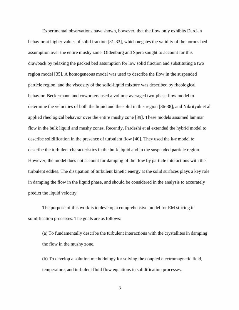
Experimental observations have shown, however, that the flow only exhibits Darcian

behavior at higher values of solid fraction [31-33], which negates the validity of the porous bed

assumption over the entire mushy zone. Oldenburg and Spera sought to account for this

drawback by relaxing the packed bed assumption for low solid fraction and substituting a two

region model [35]. A homogeneous model was used to describe the flow in the suspended

particle region, and the viscosity of the solid-liquid mixture was described by rheological

behavior. Beckermann and coworkers used a volume-averaged two-phase flow model to

determine the velocities of both the liquid and the solid in this region [36-38], and Nikrityuk et al

applied rheological behavior over the entire mushy zone [39]. These models assumed laminar

flow in the bulk liquid and mushy zones. Recently, Pardeshi et al extended the hybrid model to

describe solidification in the presence of turbulent flow [40]. They used the k-ε model to

describe the turbulent characteristics in the bulk liquid and in the suspended particle region.

However, the model does not account for damping of the flow by particle interactions with the

turbulent eddies. The dissipation of turbulent kinetic energy at the solid surfaces plays a key role

in damping the flow in the liquid phase, and should be considered in the analysis to accurately

predict the liquid velocity.

The purpose of this work is to develop a comprehensive model for EM stirring in

solidification processes. The goals are as follows:

(a) To fundamentally describe the turbulent interactions with the crystallites in damping

the flow in the mushy zone.

(b) To develop a solution methodology for solving the coupled electromagnetic field,

temperature, and turbulent fluid flow equations in solidification processes.

4

(c) To investigate the influence of crystallite size and solidification morphology on the

fluid flow—in both the bulk liquid and mushy zone—and solidification behavior during

unidirectional solidification in a bottom chill mold.

The thesis shall proceed in the following sequence. Chapter two will provide a review of

relevant literature, while Chapter three will present a solution methodology and associated

equations for computing the electromagnetic, temperature, and turbulent velocity fields. Chapter

four will present the results along with a detailed discussion, and Chapter five will briefly review

the principal findings of this work and suggest future research endeavors.

5

CHAPTER 2

LITERATURE REVIEW

In recent decades, significant strides have been made in the simulation of fluid flow, heat

transfer, and mass transfer phenomena in solidification processes as well as electromagnetic

phenomena in electromagnetic material processing systems. This chapter will provide a

recounting of previously published literature on numerical simulation of the electromagnetic,

temperature, and velocity fields in solidification systems.

2.1 Computational Electromagnetics

The electromagnetic field in EM stirring applications is typically produced using a

suitable induction coil and is represented by the well-known Maxwell equations [41]. In essence,

these equations are the differential formulation of the integral Gauss laws for conservation of

electric and magnetic fields, Ampere’s law, which relates the electric current to the magnetic

field, and Faraday’s law of induction.

Most computational techniques for calculating the EM field are based on solution of the

differential form of the Maxwell equations using potential formulations for the electric field, E,

and magnetic field, B. This is done to simplify the handling of the boundary conditions and

discontinuities in the tangential component of the electric field and the normal component of the

magnetic field. Potentials may be classified as scalar potentials or vector potentials. The most

common scalar potentials used in formulating alternating EM field problems are the electric

6

scalar potential, V, and the reduced magnetic scalar potential, Ψ. Along the same lines, the most

common vector potentials are the current vector potential, T , and the magnetic vector potential,

A. The scalar potential equations are the Laplace-Poisson type, while the governing vector

potential equations are classified as diffusion-type for time-varying EM fields.

A clear majority of formulations for eddy current problems have been based on the

magnetic vector potential, with the current vector potential coming into use more recently.

Roger and Eastham [42] used the vector potential A for the field conductor and scalar

potentials—Ψ for free space and ϕ for ferromagnetic materials—in non-conducting media. The

source field was given via the Biot-Savart law. The formulation is only applicable for singly-

connected conducting domains with uniform electrical conductivity. Furthermore, it must be

assumed that the induced field does not affect the source field. Pillsbury [43] introduced the

A,V-ϕ formulation to allow for variable electrical conductivity. In this formulation, the magnetic

and electric fields in the conducting region are determined by solving for A and V, respectively,

with ϕ being solved in free space. The use of the magnetic scalar potential in free space,

however, still means that the Pillsbury formulation may not be used for multiply-connected

domains. Roger et al [44] proposed using cuts in the conductor in the direction of the current as a

remedy to this drawback, but implementation requires special routines to deal with the

discontinuities at the cutting surfaces, increasing the computational complexity of the problem.

To handle the field in multiply-connected conducting domains, Chari et al [45] and Biddlecombe

et al [46] proposed the A,V-A formulation. This allows for the solution domain to have multiple

conductors in the domain and relaxes the need for stiff current sources, at the cost of increased

degrees of freedom.

7

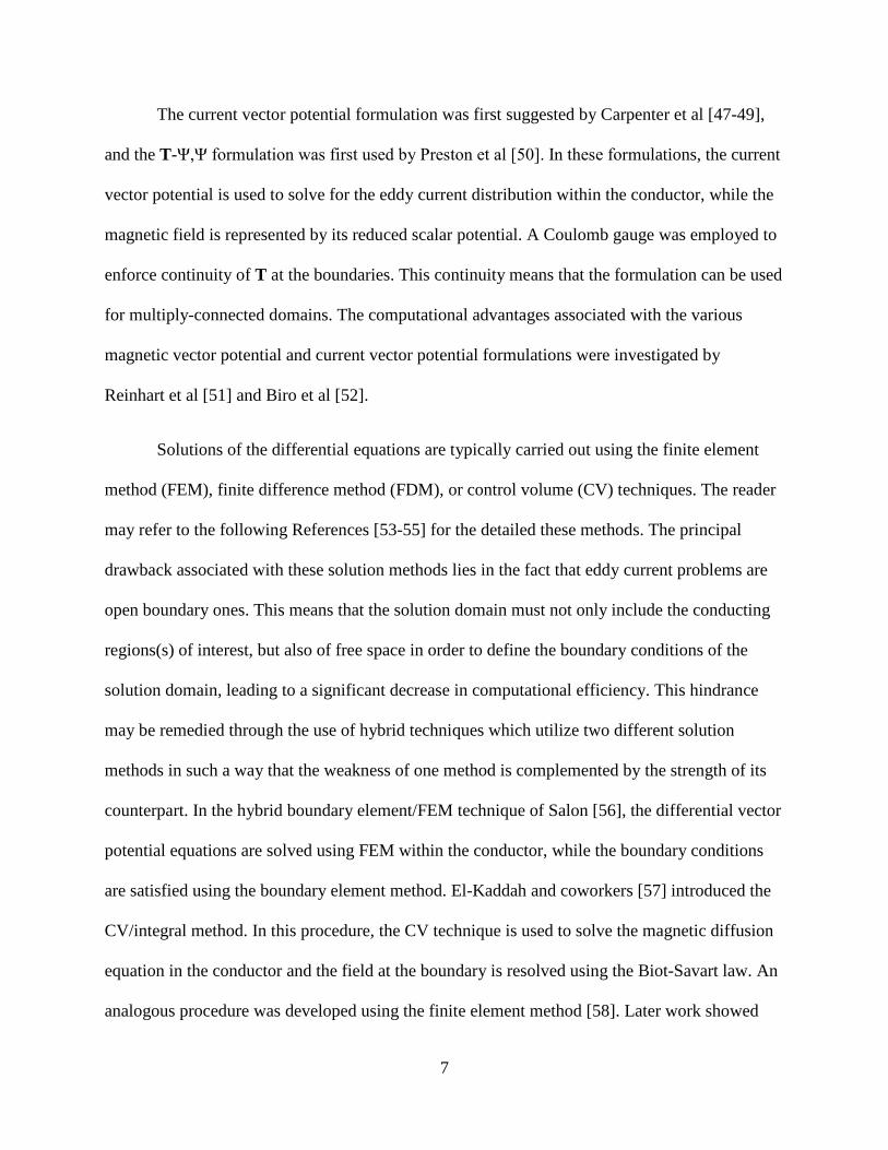
The current vector potential formulation was first suggested by Carpenter et al [47-49],

and the T-Ψ,Ψ formulation was first used by Preston et al [50]. In these formulations, the current

vector potential is used to solve for the eddy current distribution within the conductor, while the

magnetic field is represented by its reduced scalar potential. A Coulomb gauge was employed to

enforce continuity of T at the boundaries. This continuity means that the formulation can be used

for multiply-connected domains. The computational advantages associated with the various

magnetic vector potential and current vector potential formulations were investigated by

Reinhart et al [51] and Biro et al [52].

Solutions of the differential equations are typically carried out using the finite element

method (FEM), finite difference method (FDM), or control volume (CV) techniques. The reader

may refer to the following References [53-55] for the detailed these methods. The principal

drawback associated with these solution methods lies in the fact that eddy current problems are

open boundary ones. This means that the solution domain must not only include the conducting

regions(s) of interest, but also of free space in order to define the boundary conditions of the

solution domain, leading to a significant decrease in computational efficiency. This hindrance

may be remedied through the use of hybrid techniques which utilize two different solution

methods in such a way that the weakness of one method is complemented by the strength of its

counterpart. In the hybrid boundary element/FEM technique of Salon [56], the differential vector

potential equations are solved using FEM within the conductor, while the boundary conditions

are satisfied using the boundary element method. El-Kaddah and coworkers [57] introduced the

CV/integral method. In this procedure, the CV technique is used to solve the magnetic diffusion

equation in the conductor and the field at the boundary is resolved using the Biot-Savart law. An

analogous procedure was developed using the finite element method [58]. Later work showed

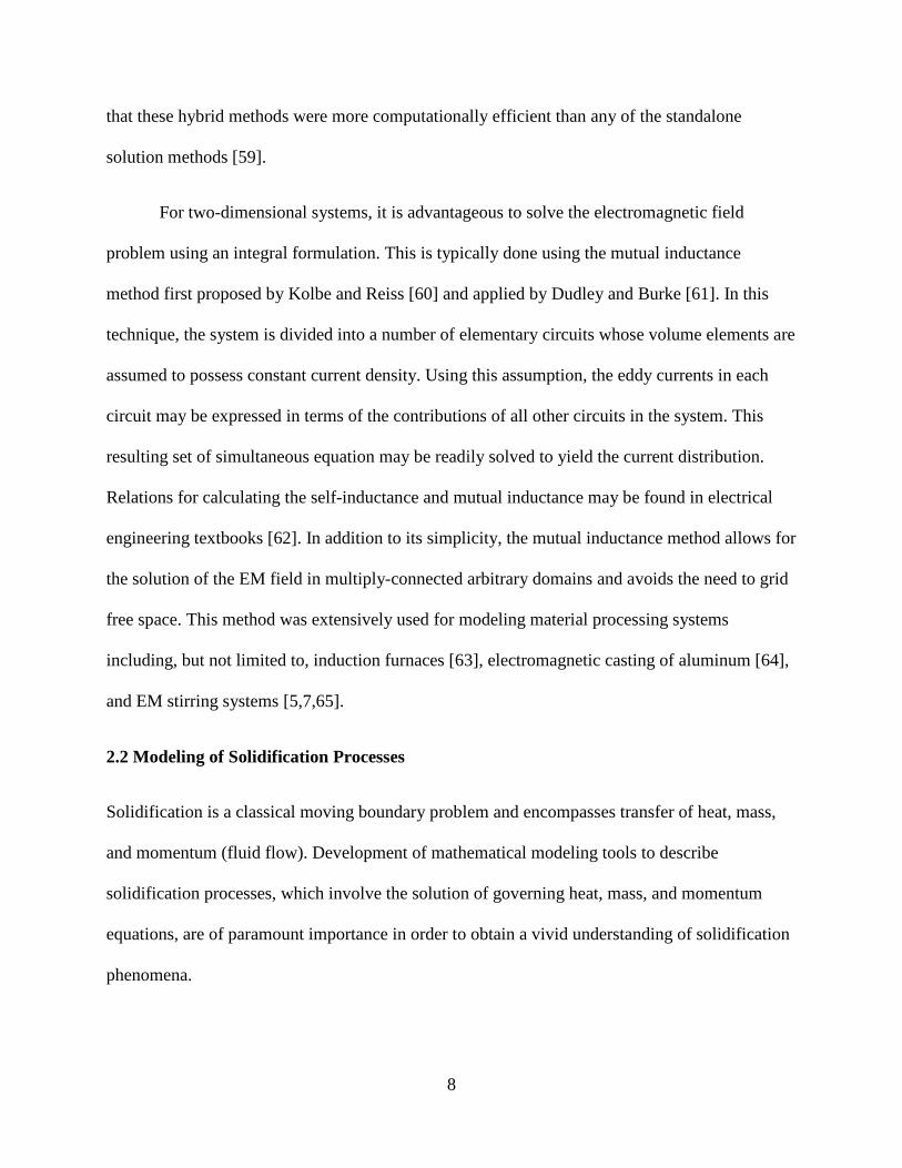
8

that these hybrid methods were more computationally efficient than any of the standalone

solution methods [59].

For two-dimensional systems, it is advantageous to solve the electromagnetic field

problem using an integral formulation. This is typically done using the mutual inductance

method first proposed by Kolbe and Reiss [60] and applied by Dudley and Burke [61]. In this

technique, the system is divided into a number of elementary circuits whose volume elements are

assumed to possess constant current density. Using this assumption, the eddy currents in each

circuit may be expressed in terms of the contributions of all other circuits in the system. This

resulting set of simultaneous equation may be readily solved to yield the current distribution.

Relations for calculating the self-inductance and mutual inductance may be found in electrical

engineering textbooks [62]. In addition to its simplicity, the mutual inductance method allows for

the solution of the EM field in multiply-connected arbitrary domains and avoids the need to grid

free space. This method was extensively used for modeling material processing systems

including, but not limited to, induction furnaces [63], electromagnetic casting of aluminum [64],

and EM stirring systems [5,7,65].

2.2 Modeling of Solidification Processes

Solidification is a classical moving boundary problem and encompasses transfer of heat, mass,

and momentum (fluid flow). Development of mathematical modeling tools to describe

solidification processes, which involve the solution of governing heat, mass, and momentum

equations, are of paramount importance in order to obtain a vivid understanding of solidification

phenomena.

9

2.2.1 Solidification in Stagnant Fluids

Initial efforts to develop a mathematical description of solidification processes were

focused on idealized problems assuming no convection in the liquid phases (i.e. stagnant liquid)

and pure materials. Such studies were later expanded to include alloy systems.

2.2.1.1 Solidification of Pure Metals

A well-known class of one dimensional solidification problems involving pure materials

is the Stefan problem. Solution of these problems requires the determination of the temperature

profile in each phase via solution of the respective conservation equations, and knowledge of the

rate of solidification front advancement, in order to resolve the Helmholtz conditions at the

interface.

Early solutions of these types of problems in one dimension were exact analytical in

form. The most renowned analytical solution is that of Neumann [66], who solved the problem

for unidirectional solidification in a semi-infinite medium using a similarity approach,

transforming the partial differential equations into ordinary ones. This is necessary due to the

non-linear nature of the energy balance at the interface. Similar solutions for radially symmetric

systems with centered line (or point) source/sink terms may be found in the work of Frank [67].

However, the assumptions and simplifications involved in obtaining an exact solution

limit their applicability with regards to bounded systems [68, 69], requiring approximate integral

methods instead. The method of Goodman [70] assumed a solid temperature fixed at the melting

point and a quadratic temperature distribution in the liquid. Lightfoot [71] examined the

unidirectional solidification of steel by treating the latent heat released as a moving heat source.

This approach was extended to two space coordinates by Rathjen and Jiji [72] for freezing of a

10

corner section and Budhia and Kreith [73] for solidification of a wedge. Although these methods

do allow for semi-analytical solutions for bounded systems, they still require a number of

simplifications. For more information on analytical methods for Stefan problems, see Rubinstein

[74].

The drawbacks of the analytical methods mentioned above have led to the development

of numerical solutions for Stefan problems in multiple space coordinates. Pure materials undergo

isothermal phase transformation and feature a sharp, distinct interface. This discontinuity may be

treated using front-tracking, boundary immobilization, or specific heat methods.

In the front-tracking approach first introduced by Murray and Landis [75], the grid

features a set of marker nodes to explicitly define the interface location, and are connected using

a piecewise function—typically a polynomial. While the grid far from the moving boundary is

fixed and regular, the grids adjacent to the solidification front are deformed and irregular in

nature. In the work by Unverdi and Tryggvason [76], an indicator function was used to define the

interface by assigning integer values to each phase. The marker nodes, defined by an interpolant,

were allowed to propagate through a fixed grid. While this method is useful in many one and

two-dimensional problems, issues arise when dealing with three-dimensional systems with

asymmetric interfaces. The level set method, developed by Osher and Sethian [77], easily

handles these complex geometries. The method relies on the determination of a level set function

that satisfies a Hamilton-Jacobi equation, where the interface is defined as the zero level set.

Implementation, however, is computationally expensive, as the level set method requires a very

fine grid structure to accurately define the interface.

11

In boundary immobilization methods, the governing heat conduction equation and the

boundary conditions are transformed into a non-orthogonal coordinate space. The interface in

this new coordinate system lies on a single, fixed coordinate surface with mobile outer

boundaries, making this a Lagrangian solution method. This method was first used for sharp

interfaces by Crank [78], and extended to two-dimensions by Duda et al [79] for phase change of

a finite, bounded cylinder. In the work by Saitoh [80], the system was mapped using the Landau

transformation, thereby reducing the number of space variables by one. Each of these studies

used the finite difference method to achieve solution. Hsu et al [81], on the other hand, used the

control volume technique to solve the transformed equations. Although the boundary

immobilization method has been shown to produce accurate solutions of benchmark problems

[82], the transformed conservation equations contain highly nonlinear cross-derivative terms

consisting of more than one space variable, which make implementation cumbersome.

The specific heat method, first introduced by Thionov and Samarskii [83], seeks to avoid

the need to explicitly discretize the boundary by introducing an effective specific heat capacity

near the transformation temperature. This is accomplished by assuming that the discontinuity in

enthalpy can be represented by a very narrow freezing range. This allows for the heat conduction

equation to be rewritten in terms of a piecewise function to represent the specific heat. A

thorough introduction to the method, along with examples, may be found in Szekely and

Thelimis [84]. The first applications of this method comes from Soviet literature via the works of

Budak et al [85] and Samarskii and Moisyenko [86] for generalized Stefan problems. For pure

materials, the latent heat evolution is assumed to be linear with respect to temperature.

12

2.2.1.2 Solidification of Alloys

In alloy systems, the phase transition is not isothermal, but rather occurs over a

temperature range, the extent of which may be ascertained through use of a phase diagram. Alloy

solidification begins at the liquidus temperature, and may be regarded as complete at the solidus

temperature. The incremental nature of this phase change makes application of front-tracking

and boundary immobilization methods impractical.

For alloy solidification, latent heat evolution is depended on transformation kinetics. At

the macro-level, this can be represented through the rate of change of solid fraction, which is

typically given as a function of temperature. This allows for the use of the specific heat method

[87]. A number of functions have been developed to represent the solid fraction. The simplest is

assuming the solid fraction obeys a linear relationship with temperature, and is used in the works

of Voller and Prakash [24] and Poole et al [88], among others. For equilibrium solidification

with solute segregation, the lever rule is used [89]; the partition coefficient is assumed constant

for nearly-linear solidus and liquidus lines. For non-equilibrium solidification, the Schiel

equation is typically used [90]. In addition, the solid fraction may also be defined as a piecewise

function using experimental solidification curves. Examples of this method are given in Carlson

and Beckermann [91] and Li et al [92].

2.2.2 Solidification Models with Fluid Flow

The stagnant fluid assumption from early formulations makes for a simpler solution of

solidification problems. Experimental observations, however, make validity of this assumption

rare, as the presence of fluid flow and convective heat and mass transfer causes significant

deviation from diffusion-only solutions. Such convective phenomena have been shown to have a

13

strong influence on the microstructure and segregation profiles of the final product [5-10, 15, 17-

20, 93].

Convective transport is generally categorized into two regimes: natural convection and

forced convection. In natural convection, fluid flow occurs as a result of density differences

stemming from thermal gradients in the liquid and solute rejection at the interface. The intensity

of natural convection is defined by the Rayleigh number, which describes the relative strength of

the buoyancy and viscous forces. Theoretical studies [94-96] determined the critical value of the

Rayleigh number for the onset of natural convection in alloys to be on the order of 104.

Experimental work [97-99] found that convection in aqueous alloy analogues significantly alters

the solidification velocity and the curvature of the melt front, both important parameters in

determining the solidification morphology and grain size [100]. The work by Stewart [101] using

radioactive tracers in the Al-Ag alloy system found natural convection to play a substantial role

in macrosegregation.

Forced convection occurs through application of body forces via an external source

which may be mechanical [102], ultrasonic [103], or electromagnetic [1-5] in form. The effects

of forced convection on the micro/macrostructure are well-documented. Liu et al [104] found

that forced convection homogenized the alloying elements in the liquid and improved solution

strengthening of AZ91 magnesium specimens. Kuznetzov [105] found considerable inverse

segregation of carbon in twin-roll cast steels. Most important is the role of stirring on grain

refinement through dendrite fragmentation and transport, which increases the nucleation

potential in the melt [15-20].

14

It is important to note that convection, regardless of the source, is found not only in the

bulk liquid, but in the mushy zone as well [32-34, 106]. Several formulations characterizing the

flow in the mushy zone have been developed, and may be fundamentally classified as either

single-zone or dual-zone models.

2.2.2.1 Single-Zone Models

The first single-zone model was that by Mehrabian et al [107] to describe the role of

interdendritic flow on solute redistribution. The entire mushy zone was assumed to behave as a

porous medium that obeys Darcy’s law, with the permeability given by the Hagen-Poiseuille

relation. Although the model was found to be in agreement with experimental work with ternary

alloys [108], the solution domain was limited to the mushy zone only. Szekely and Jassal [109]

later expanded the solution domain to include both the bulk liquid and the mushy zone.

The extent of momentum damping in Darcy flows is dependent on the permeability of the

medium, which is expressed in terms of the flow intensity and the geometry of the interdendritic

network. For macro-scale models, the permeability is taken as isotropic due to the randomness of

the dendrite orientations [110]. A number of permeability models have been proposed. The

Hagen-Poiseuille model describes the permeability through friction loss in laminar flow through

a tube [111], and is a good approximation for columnar solidification. The Hagen model was

commonly used in the works of Mehrabian and his coworkers [22, 23, 108] and by Poirier and

coworkers [112-114]. For equiaxed and globular morphologies, the permeability is most

commonly given by the Kozeny family of equations (e.g. Carman-Kozeny [27] and Blake-

Kozeny [112]). These assume laminar flow through array of packed spheres. Kozeny

15

relationships may be found in Voller and Prakash [24], Incropera and coworkers [25,30], and

Campanella et al [26], among many others.

Due to the irregular nature of dendrites, analyses correlating the permeability to the

dendrite arm spacing have been performed. Poirier [28] did a regression analysis of the data from

experimental permeability measurements (see References [33,34,115,116]), and expressed the

Hagen-Poiseuille and Blake-Kozeny equations in terms of the primary dendrite arm spacing and

a coefficient dependent on the grain tortuosity. The tortuosity has been described in terms of a

power series with respect to the ratio of the primary arm spacing to its secondary counterpart

[117], or in terms of a shape factor [118].

The previously-mentioned single-zone models were for laminar flow only. There have

been some efforts to account for turbulence in the mushy zone. Shyy et al [29] were the first to

incorporate turbulence in the single-zone model. To account for the effect of momentum

damping on the turbulent characteristics of the flow, a k-ε model for low Reynolds number flows

was used. However, the formulation did not account for the added dissipation due to interaction

between the turbulent eddies and the solid phase [119], and only gave the turbulence constant Cμ

a functional dependence, leaving the constants associated with the source and sink terms

unchanged from that for bulk flow. This ad-hoc approach prevents turbulent closure of k and ε.

Prescott and Incropera [30] later attempted to define the turbulent flow field for an EM stirred

system using the k-ε model of Jones and Launder [120], and reported significant damping of

turbulence in the mushy zone. Although turbulent closure is attained, the researchers incorporate

a Darcy term in the k and ε equations that does not reflect the physics of the problem, as Darcy’s

law only applies to laminar flow. Furthermore, the assumption of turbulent flow in both models

is incompatible with the porous medium model, as the turbulent mixing length is larger than the

16

pore size, which is on the order of microns. Such mixing lengths are on the Kolomogrov scale,

making the flow essentially laminar with regards to the macro-scale [121].

2.2.2.2 Dual-Zone Models

While single-zone models have proven useful in describing the interdendritic/mushy zone

flow for castings exhibit columnar solidification morphology, use of the porous medium

assumption over the entire mushy region is not physically valid for equiaxed solidification

structures. Experimental investigations [17,18] have shown that equiaxed crystallites and

dendrite fragments may not be regarded as stationary, as assumed in Darcy’s law and associated

permeability relations, but rather travel with the flow current at low solid fraction. Further work

[33,34] has shown that Darcian behavior only occurs at higher solid fractions, where the

dendrites have formed an interlocking, immobile mesh.

This presents a need for a dual-zone model to account for the varying behavior of the

crystallites with respect to solid fraction. West [122] attempted to account for the behavior of the

free crystallites by assuming the existence of two packed bed regions with distinct

permeabilities, and was found to be in good agreement with the experimental findings of

Piwonka and Flemings [107]. However, this approach still assumes a fixed particle arrangement

for the crystallites at low solid fraction, not consistent with the actual physical phenomena, and

may not be used for turbulent flow for reasons previously mentioned.

To accurately account for the mobility of free crystallites, the dual-zone formulation of

Oldenburg and Spera [35] relaxed the packed bed assumption for the region predominated by

free crystallites, forming a suspended particle region. This region, which consists of equiaxed

crystallites and fragments, are treated in aggregate using a homogeneous two-phase flow with the

17

viscosity described by the rheological behavior of slurries. Darcy’s law was used for the region

where the crystallites have settled and formed a coherent network of stationary particles. The

Oldenburg-Spera approach was used by Chang and Stefanescu [123] for modeling of

macrosegregation of Al-Cu alloys, and by Mat and Ilegbusi [124,125] for describing

macrosegregation in an aqueous alloy analogue under buoyancy-driven flow. This formulation

correctly reflects the observed solidification phenomena for equiaxed structures, but is limited

only to laminar flow; in contrast, the flow in EM stirred systems is typically turbulent [1,57].

Recently, Pardeshi et al [40] presented a dual-zone formulation that accounts for

turbulent behavior in EM stirring systems. In the suspended particle region, the viscosity is given

by an empirical relationship, with the Carman-Kozeny relation accounting for the permeability in

the fixed particle region. The turbulent characteristics of the flow were determined using the

high-Re k-ε model of Launder and Spalding [126] throughout the bulk liquid and the mushy

zone. While this represented a significant advancement towards understanding turbulent

convective transport in an equiaxed mushy zone, a number of assumptions conflict with physical

reality. First, the model suffers from the same mixing length drawback as those of Prescott and

Incropera [30] and Shyy et al [29] in calculating the turbulent characteristics in a solidifying

porous medium, making turbulent closure unattainable. Furthermore, it does not account for

momentum damping, along with laminarization of the flow, in the suspended particle region due

to particle interactions with the turbulent eddies. Budenkova et al [31] recently attempted to

account for the particle interactions, but used an ad-hoc expression which lacks any physical

foundation.

18

CHAPTER 3

MODEL FORMULATION

This chapter presents a two-dimensional formulation and solution methodology for

describing the coupled electromagnetic field, fluid flow, and heat transfer phenomena during

solidification in electromagnetically stirred systems.

3.1 Statement of the Problem

Figure 3.1 shows a typical casting system in which the molten metal is stirred by an

electromagnetic field. In essence, it consists of a heat extraction device (mold) and an

electromagnetic stirrer—typically an induction coil. Heat extraction occurs through the

refractory walls, the water-cooled chill plate, or a combination of both. Solidification takes place

as a result of heat transfer from the bulk metal to the mold walls. This produces a temperature

gradient ranging from the melt temperature to the temperature at the walls, which results in the

formation of a solid layer, a liquid layer, and a mushy zone, where the temperature lies between

the solidus and liquidus temperatures and the solid and liquid phases coexist in. The shape and

thickness of each individual layer for any given time depends on the structure and magnitude of

the flow— which is driven by buoyant and/or electromagnetic (Lorentz) forces resulting from

19

density gradients and the interaction between the current and magnetic field generated by the

induction coil in the system, respectively.

In order to develop a fundamental understanding of the solidification phenomena in the

mold, one needs to describe the temperature, velocity, and electromagnetic fields. This requires

calculation of the electromagnetic field over the entire system, the temperature field in the metal,

and the velocity field in both the bulk liquid and the mushy zone.

Figure 3.1. Sketch of EM stirred melt undergoing solidification

3.1.1 The Electromagnetic Field Problem

The system shown in Figure 3.1 is just a simple example of an EM stirred system;

however, the principles are the same for any two-dimensional EM stirred solidification system.

Eddy currents are generated by passing a current through the induction coil, which interacts with

the accompanying magnetic field, creating Lorentz forces in the liquid; the rotational part of

20

these forces drive fluid motion in the molten metal. Furthermore, the eddy currents generate heat

through electrical energy dissipation. It is important to note, however, that the magnetic field

characteristics depend not only on interactions with the metal, but with adjacent conducting

materials such as the chill block and/or magnetic shields. These additional components must be

considered in any analysis of the electromagnetic field phenomena.

3.1.2 Heat Transfer Problem

Solidification occurs by heat extraction through the water-cooled chill block located at

the base of the metal specimen. The metal is jacketed by a refractory tube, minimizing heat

losses from the sides allowing for unidirectional solidification. In the developed model, the metal

is represented by three distinct domains: the bulk liquid, the mushy zone, and the solid. Unlike

quiescent melts, heat transfer in the bulk liquid is not limited to conduction only, but occurs by

convection as well. In the mushy zone, both transport modes still persist, albeit with additional

release of latent heat whose evolution depends on the solid fraction, fs. Upon complete

solidification, heat transfer is restricted to conduction only.

3.1.3 Fluid Flow Problem

The presence of the convective regime in the heat transfer problem by convection

necessitates the characterization of the velocity field. While the process of defining the flow in

the bulk liquid is well-known, the flow characteristics of the mushy zone are dependent on the

interactions between the solid and liquid phases. To describe these interactions, the mushy zone

was represented by two distinct regions, as shown in Figure 3.2. At values of low fs, newly-

formed crystallites and dendrite fragments move freely with the flow, forming a slurry, and is

referred to as the suspended particle region. As the crystallites grow, they settle and coarsen into

an interlocking network resembling a packed bed. This is referred to as the fixed particle region.

21

In the suspended particle region, the velocity is damped due to interactions between the

turbulent eddies and the solid particles at the liquid-particle interface. In the fixed particle region,

damping of the flow occurs due to the existence of an increasingly constricted flow path, which

may be described in terms of the permeability. Lorentz forces are also affected. In the suspended

particle region, electromagnetic forces are unaffected by the presence of crystallites, but may be

neglected in the fixed particle region, as the solid is unable to be deformed by the forces. In this

region, the flow is driven by buoyancy effects.

The proceeding sections will define the relevant conservation equations for the

electromagnetic, temperature, and velocity fields for each domain, followed by the method of

solution for these equations.

Figure 3.2. Illustration of the various flow domains

22

3.2 Formulation of the Electromagnetic Field

3.2.1 Governing Equations

The electromagnetic field is governed by the well-known Maxwell equations, which are the

differential forms of Ampere’s law and Faraday’s law, together with constitutive equations

describing the relationships between the current, electric field, and magnetic field. Using the

magnetohydrostatic assumption—typically appropriate for nonmagnetic materials—Ohm’s law

is expressed as

𝑱 = 𝜎𝑬 (3.1)

where σ is the electrical conductivity of the metal, J is the current density, and E is the electric

field intensity. The Lorentz force, Fem, may be expressed as

𝑭𝒆𝒎 = 𝑱 × 𝑩 (3.2)

where B is the magnetic flux density. The electrical energy dissipation (Joule heating) is given in

terms of the magnitude of J and the conductivity:

𝑆𝑒𝑚 = 𝑱�̅�𝜎

(3.3)

3.2.2 Numerical Solution of the Electromagnetic Field

As previously mentioned in Chapter 2, two common techniques to compute the electric

and magnetic fields are differential and mutual inductance methods. In this study, the mutual

inductance method was used due to its ability to easily handle the electromagnetic field equations

in systems with noncontiguous components.

Due to the axisymmetric nature of the problem shown in Figure 3.1, current flow in the θ-

direction, the time-harmonic J and B fields may be written in phasor form as

𝑱 = 𝑅𝑒{𝐽𝜃𝑒𝑥𝑝[𝑗𝜔𝑡]}𝜃� (3.4)

𝑩 = 𝑅𝑒{𝑩𝑒𝑥𝑝[𝑗𝜔𝑡 + 𝜑]} (3.5)

23

Here, j is the square root of -1, ω is the angular frequency of the inductor, and φ is the phase

angle. Fem and Sem are given as

𝑭𝒆𝒎 = 12𝑅𝑒{𝑱 × 𝑩} (3.6)

𝑆𝑒𝑚 = 12𝑅𝑒 �𝑱�̅�

𝜎� (3.7)

where the bar denotes the complex conjugate of the vector.

The mutual inductance method utilizes the integral form of the Maxwell equations. From

Ampere’s law the B field at r due to a current at point r’ may be given by

𝑩(𝒓) = 𝜇04𝜋 ∮

𝑱×(𝒓−𝒓′)|𝒓−𝒓′|3𝑣𝑜𝑙 𝑑𝑣 (3.8)

where μ0 is the magnetic permeability of free space. It is possible to express the previous

equation in terms of the magnetic vector potential, A, as

𝑨(𝒓) = 𝜇04𝜋 ∮

𝑱|𝒓−𝒓′|

𝑑𝑣𝑣𝑜𝑙 (3.9)

where

𝑩 = 𝛁 × 𝑨 (3.10)

To evaluate A, the metal, induction coil, and other conducting components may be

subdivided into a number of simple circuits which are assumed to have constant current density.

A can then be expressed in terms of the individual current densities

𝐴𝜃(𝒓) = 𝜇04𝜋�∑ (𝑱.𝑺)𝑚 ∮

𝒅𝒍𝑚|𝒓−𝒓′𝒎|

𝑚𝑒𝑡𝑎𝑙𝑚=1 + ∑ (𝑱.𝑺)𝑐 ∮

𝒅𝒍𝑐|𝒓−𝒓′𝒄|

𝑐𝑜𝑛𝑑𝑐=1

+∑ 𝐼𝑘 ∮𝒅𝒍𝑘

|𝒓−𝒓′𝒌|𝑐𝑜𝑖𝑙𝑘=1

� (3.11)

where Ik is the applied current in each turn of the induction coil.

Through use of Faraday’s law of induction, each individual current, Ji, may be expressed

with respect to the current densities in all other elements.

∮ 𝑱𝑖.𝑑𝒍𝑖 = −𝑗𝜔𝜎�∑ 𝑀𝑖,𝑚(𝑱.𝑺)𝑚𝑚𝑒𝑡𝑎𝑙𝑚=1 + ∑ 𝑀𝑖,𝑐(𝑱.𝑺)𝑐𝑐𝑜𝑛𝑑

𝑐=1 ∑ 𝑀𝑖,𝑘𝐼𝑘𝑐𝑜𝑖𝑙𝑘=1 � (3.12)

24

where dl is the length of the circuit, S is the cross-sectional area of the cell, and Mi,k is the mutual

inductance given by

𝑀𝑖,𝑘 = 𝜇04𝜋∯

𝑑𝒍𝑘.𝑑𝒍𝑖𝑟′

(3.13)

Applying Equation (3.12) to the each circuit, a set of simultaneous equations is obtained. The

resulting matrix is symmetric and positive definite, and may be solved using Choleski

factorization. Upon obtaining the J field, Ampere’s law is used to obtain B.

3.3 Governing Equations for the Heat Transfer Problem

As previously mentioned, the solidification rate depends on the rate of heat extraction

from the metal. The differential energy equation is given by

𝜌𝑐𝑝𝜕𝑇𝜕𝑡

+ 𝜌𝑐𝑝𝒖.∇𝑇 = ∇. (𝑘𝑒∇𝑇) + 𝑆𝑒𝑚 + 𝑆𝐿 (3.14)

where ρ, cp, and ke are the density, specific heat capacity, and effective thermal conductivity,

respectively, and u is the fluid velocity. Sem is the electrical energy dissipation per unit volume

given in Equation (3.3). SL corresponds to the release of latent heat and is given as

𝑆𝐿 = 𝜌𝐿 𝜕𝑓𝑠𝜕𝑡

+ 𝜌𝐿𝒖.∇𝑓𝑠 (3.15)

where L is the latent heat of fusion. The first term in Equation (3.15) describes the latent heat

released due to growth kinetics, while the second term accounts for the latent heat released by

advected crystallites. Assuming the linear evolution of solid fraction with respect to temperature,

fs is given by

𝑓𝑠 = �0 𝑖𝑛 𝑡ℎ𝑒 𝑙𝑖𝑞𝑢𝑖𝑑

𝑇𝐿−𝑇𝑇𝐿−𝑇𝑆

𝑖𝑛 𝑡ℎ𝑒 𝑚𝑢𝑠ℎ𝑦 𝑟𝑒𝑔𝑖𝑜𝑛

1 𝑖𝑛 𝑡ℎ𝑒 𝑠𝑜𝑙𝑖𝑑

� (3.16)

where TL is the liquidus temperature and TS is the solidus temperature. By evaluating the

derivatives in the SL equation, Equation (3.15) can be rewritten as

25

𝑆𝐿 = −𝜌 𝐿𝑇𝐿−𝑇𝑆

�𝜕𝑇𝜕𝑡

+ 𝒖.𝛁𝑇� (3.17)

Noting that L/TL-TS is the specific heat of fusion and that the bracketed term is the material

derivative of T, the conservation equation, Equation (3.14), can be expressed as

𝜌𝐶∗ 𝐷𝑇𝐷𝑡

= ∇. (𝑘𝑒∇𝑇) + 𝑆𝑒𝑚 (3.18)

where C* is the apparent heat capacity, given by

𝐶∗ = �

𝑐𝑝,𝑙 𝑖𝑛 𝑡ℎ𝑒 𝑙𝑖𝑞𝑢𝑖𝑑

𝑐𝑝,𝑙 + 𝐿𝑇𝐿−𝑇𝑆

𝑖𝑛 𝑡ℎ𝑒 𝑚𝑢𝑠ℎ𝑦 𝑧𝑜𝑛𝑒

𝑐𝑝,𝑠 𝑖𝑛 𝑡ℎ𝑒 𝑠𝑜𝑙𝑖𝑑

� (3.19)

The effective thermal conductivity depends on the domain. In the solid, the ke is equal to

its molecular value, ks; for the mushy zone, regardless of region, it is assumed that ke obeys the

following mixture rule:

𝑘𝑒 = 𝑓𝑠𝑘𝑠 + (1 − 𝑓𝑠)𝑘𝑙 (3.20)

For the bulk liquid, the value of ke is depends on the turbulent characteristics of the flow, and is

given by

𝑘𝑒 = 𝑘𝑙 + 𝜇𝑡𝑐𝑝,𝑙

𝑃𝑟 (3.21)

The variables μt and Pr correspond to the turbulent viscosity (see Section 3.4) and the Prandtl

number, respectively.

3.4 Formulation of the Fluid Flow Model

Since the fluid flow and heat transfer equations are strongly coupled by convection, the

velocity must be properly described in both the bulk liquid and mushy zone. Because the flow

behavior varies in each domain, each described in Section 3.1.3, this section will describe the

models used for each individual domain.

26

3.4.1 Conservation Equations for Fluid Flow

Fluid flow in the bulk liquid is given by the classical Navier-Stokes and continuity

equations for incompressible fluids

𝜌 𝝏𝒖𝝏𝑡

+ 𝜌𝒖.∇𝒖 = −∇P + (𝜇𝑙∗ + 𝜇𝑡)∇2𝒖 + 𝑭𝑒𝑚 + 𝑭𝑏 (3.22)

𝛁.𝒖 = 0 (3.23)

where u is the velocity vector, P is the pressure, μl* is the effective laminar viscosity, and Fem and

Fb representing the Lorentz and buoyancy body forces, respectively. The effective viscosity may

be given through the turbulent and laminar components. The turbulent viscosity component is

given by the k-ε model, which will be discussed in further detail in a later subsection.

To describe fluid flow in the two-phase mushy zone, the velocity vector is defined

through the weighted contribution of the solid and liquid phases with respect to solid fraction.

𝒖 = 𝒖𝑠𝑓𝑠 + 𝒖𝑙(1 − 𝑓𝑠) (3.24)

The physical properties are described in a similar manner as Equation (3.24). The subscripts s

and l represent the solid and liquid phases, respectively.

The flow in the suspended particle region is described by the homogeneous two-phase

flow model. In this model, the solid crystallites and the liquid are considered to have nearly equal

density, and thus are aggregated into a pseudofluid. This allows for the time-averaged velocities

of the solid and liquid phases to be assumed equal (ūl ≡ ūs). The conservation equations for the

time-averaged velocity of the pseudofluid are similar in form to the Navier-Stokes equation

given in Equation (3.22).

𝜌 𝝏𝒖𝝏𝑡

+ 𝜌𝒖.∇𝒖 = −𝛻𝑃 + (𝜇𝑙∗ + 𝜇𝑡)𝛻2𝒖 + 𝑭𝑒𝑚 + 𝑭𝑏 + 𝑭𝑑 (3.25)

27

The continuity equation for the suspended particle region is identical to Equation (3.23).

The additional term, Fd, is a body force that damps the flow due to the presence of the solid

phase, and will be described later in further detail.

In the fixed particle region, defined by fc<fs<1 (where fc represents the coherency solid

fraction), the solid crystallites are interlocked among each other. Therefore, the velocity of the

solid is held to be identically zero (us=0), giving ul=u/fl. Furthermore, the solid network prevents

the application of Lorentz forces within the liquid phase, making Fem equal to zero. The modified

Navier-Stokes equation is given by

𝜌 𝝏𝒖𝝏𝒕

+ 𝜌𝑓𝑙𝒖.𝛻𝒖 = −𝛻𝑃 + 𝜇𝑙∗𝛻2𝒖 + 𝑭𝑏 + 𝑭𝑑 (3.26)

As with the other two flow regions, the continuity equation is again given by Equation

(3.22). Note that the turbulent viscosity term no longer appears behind the vector Laplacian as it

is assumed that turbulence is completely damped in the interdendritic channels. This assumption

is reasonable since the spacing between crystallite arms is less than or equal to the Taylor mixing

length used in the k-ε models.

3.4.2 Description of Source Terms in the Conservation Equations

To describe the buoyancy force, Fb, over the three flow regions in terms of temperature,

the linear Boussinesq approximation is used

𝑭𝑏 = 𝜌0[1 − 𝛽(𝑇 − 𝑇0)]𝒈 (3.27)

where β is the volume coefficient of thermal expansion. The naught terms in Equation (3.27), ρ0

and T0, represent the reference density and temperature, respectively; in this work, the values are

given as those of the bulk liquid.

The expression for the damping force, Fd, is dependent on the flow region in question,

with the extent of damping dependent on the solid fraction. In the suspended particle region, the

28

damping is due to the crystallite interactions with the turbulent eddies, while in the fixed particle

region the damping is given by the pressure drop due to Darcy’s law. These are represented

below in Equation (3.28).

𝑭𝒅 = �−2𝜌√6𝑘𝐼𝑇𝑓𝑠1−𝑛𝑓𝑐𝑛

𝐷𝑔𝒖 ∀𝑓𝑠 ∈ (0,𝑓𝑐)

−𝜇𝑙∗

𝐾𝒖 ∀𝑓𝑠 ∈ [𝑓𝑐 , 1]

� (3.28)

In the expression for the suspended particle domain, k represents the turbulent kinetic energy, IT

is the turbulent intensity, Dg is the grain size, and n is a grain growth exponent ranging from zero

to one dependent on the crystallite growth kinetics. In the fixed particle region, K represents the

permeability of the interdendritic medium, and is given by the well-known Carman-Kozeny

equation. A derivation of the damping force in the suspended particle region resulting from

turbulent interactions is given in subsection 3.4.4.

The effective laminar viscosity is also dependent on the behavior of the solid crystallites

in each flow domain. In the bulk liquid and fixed particle regions, the viscosity is given by the

molecular value only; in the suspended particle region, however, the particles serve to induce

rheological behavior in the pseudofluid, which is given by the Mooney equation [127]. The

expression for the effective laminar viscosity over all values of solid fraction is given by

𝜇𝑙∗ =

⎩⎪⎨

⎪⎧ 𝜇0∗ 𝑓𝑠 ≡ 0

𝜇0∗𝑒𝑥𝑝 �2.5𝑓𝑠

1−𝑓𝑠 0.68�� ∀𝑓𝑠 ∈ (0,𝑓𝑐)

𝜇0∗ ∀𝑓𝑠 ∈ (𝑓𝑐, 1)

� (3.29)

where μ0* in the above equation is the molecular viscosity of the material

3.4.3 Low-Re Turbulence Model for Homogeneous Flow

For single-phase flows in domains consisting of fixed boundaries, the turbulent

characteristics of the flow are described using the k-ε model developed by Launder and Spalding

29

[126], along with appropriate representations of the viscous sublayer near the walls. In a two-

phase region where one of the phases is solid and assumed undeformable, the Launder-Spalding

model cannot accurately describe the effects regarding the presence of the solid phase on the

turbulent field using the traditional wall functions. Instead, the turbulent characteristics are

described by a k-ε model adapted for low-Re flows by Jones and Launder [120]. Assuming

isotropic turbulent behavior, the equations for the turbulent kinetic energy and turbulent energy

dissipation are given by

𝜌 𝜕𝑘𝜕𝑡

+ 𝜌(𝒖.∇)𝑘 = ∇. �𝜇𝑡𝜎𝑘∇𝑘�+ 𝐺 − 𝜌𝜀 (3.30)

𝜌 𝜕𝜀𝜕𝑡

+ 𝜌(𝒖.∇)𝜀 = ∇. �𝜇𝑡𝜎𝜀∇𝜀�+ 𝐶1

𝜀𝑘𝐺 − 𝐶2

𝜀2

𝑘 (3.31)

In these equations, C1 and C2 are functions dependent on the intensity of the flow. G represents

the turbulent shear generation term, and is written below in abbreviated tensor form.

𝐺𝑖𝑗 = 𝜇𝑡 �𝜕𝑢𝑖𝜕𝑥𝑗

+ 𝜕𝑢𝑗𝜕𝑥𝑖� 𝜕𝑢𝑖𝜕𝑥𝑗

(3.32)

Given the values of the turbulent kinetic energy and the turbulent energy dissipation rate, the

turbulent viscosity is given by

𝜇𝑡 = 𝐶𝜇𝜌𝑘2/𝜀 (3.34)

Cμ is defined as the drag coefficient and, like C1 and C2, has a functional dependence with

respect to the flow intensity

In describing the functions for C1, C2, and Cμ, necessary to ensure closure of the

turbulence problem, the flow intensity is conveniently described as a ratio of the turbulent

viscosity to the molecular viscosity of the bulk liquid, referred to as the turbulent Reynolds

number, RT=ρk2/μl*ε. The functions by are given by Jones and Launder [120] as

30

𝐶1 = 1.44 (3.36)

𝐶2 = 1.92�1 − 0.3𝑒𝑥𝑝(−𝑅𝑇2)� (3.37)

𝐶𝜇 = 0.09𝑒𝑥𝑝 �−3.4

1+𝑅𝑇50� (3.38)

It is important to note that at high values of RT, the functions are equal to the prefactors in each

equation

3.4.4 Determination of the Damping Force

To determine the damping force in the suspended particle region (from Equation (3.28)),

consider a volume element containing N particles and occupying a total volume V. Consistent

with the homogeneous flow model, let the time-averaged velocities of each phase in the volume

element be identically equal to one another (ūl ≡ ūs). Furthermore, assume that the turbulent

fluctuations be confined to the liquid only (i.e. u’s ≡ 0). For this to be valid, the volumetric drag

force Fd must be equal to the sum of the Reynolds stresses at the particle surface; that is

∭ 𝑭𝒅𝑑𝑉𝑉 = ∯ 𝝉𝒕�𝐴𝑝.𝒏�𝑑𝑆 (3.37)

where ñ is the unit normal to the cross-section of the flow. The time-averaged Reynolds stress is

given in tensor form as

𝝉𝒕� = −𝜌𝑢′𝚤𝑢′𝚥������� (3.38)

Assuming isotropic turbulence, this equation may be rewritten in terms of the turbulent kinetic

energy, k, and the unit tensor, I [121].

𝝉�𝒕 = −23𝜌𝑘𝑰 (3.39)

Therefore

𝑭𝑑𝑉 = ∯ 𝝉𝒕�𝐴𝑝.𝒏� 𝑑𝑆 = −2

3𝜌𝑘𝐴𝑝

𝒖|𝒖| (3.40)

31

Let Ap be the sum of the surface areas of all the particles in the control volume. For uniform

particle size with respect to solid fraction, Ap=πdg2N. The number of particles in the control

volume is given by

𝑁 = 𝑡𝑜𝑡𝑎𝑙 𝑚𝑎𝑠𝑠 𝑜𝑓 𝑡ℎ𝑒 𝑠𝑜𝑙𝑖𝑑𝑚𝑎𝑠𝑠 𝑜𝑓 𝑜𝑛𝑒 𝑝𝑎𝑟𝑡𝑖𝑐𝑙𝑒

= 6𝑓𝑠𝑉𝜋𝑑𝑔3

(3.41)

where dg is the particle diameter of the equivalent sphere, and is a function of solid fraction. This

gives

𝐴𝑝 = 6𝑓𝑠𝑉𝑑𝑔

(3.42)

Inserting this relation into (3.40) gives

𝑭𝑑 = −4𝜌𝑘𝑓𝑠𝑑𝑔|𝒖| 𝒖 (3.43)

The turbulent intensity, IT, is defined by

𝐼𝑇 = �2𝑘3

|𝒖|−1 (3.44)

The force is then rewritten as

𝑭𝒅 = −2√6𝜌√𝑘𝐼𝑇𝑓𝑠𝑑𝑔

𝒖 (3.45)

Let dg is defined in terms of a power law

dg = A0fsn + B0 (3.46)

where A0 and B0 are grain growth constants. For dg = 0 at fs = 0 and dg = D at fs = fc, where D is

the final grain size and fc is the coherency solid fraction, (3.46) becomes

dg = Dg(fs/fc)n (3.47)

This gives the final form of the damping force per unit volume used in Equation (3.xx).

𝑭𝒅 = −2√6𝜌√𝑘𝐼𝑇𝑓𝑠1−𝑛𝑓𝑐𝑛

𝐷𝑔𝒖 (3.48)

32

3.5 Numerical Solution of the Transport Equations

To solve the governing equations, for the transport quantities, the control volume method

was used. In the control volume method, the metal domain is subdivided into a number of cells

bounded by constant values of r and z called control volumes. In each control volume, the value

of the transport quantity is presumed to dominate over the entire cell.

Since the conservation equations all follow a similar template, the canonical form of the

conservation equation for general variable ϕ is given by

𝜌 𝜕𝜙𝜕𝑡

+ 𝜌𝒖.∇𝜙 = ∇. (Γ𝜙∇𝜙) + 𝑆𝜙 (3.49)

where Γϕ and Sϕ are the variable-dependent diffusion coefficient and source terms.

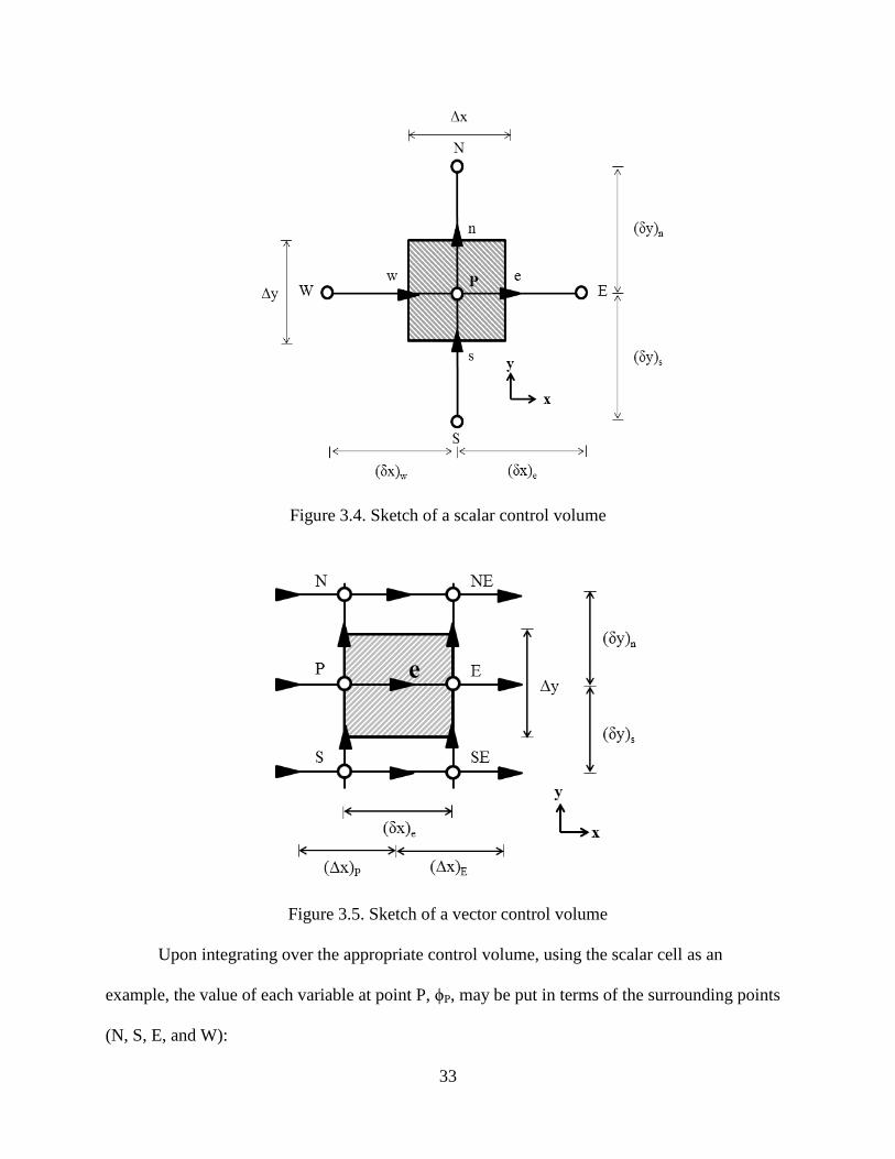
To account for the coupling between the pressure and the velocity, a staggered-grid approach is

used. An illustration of this grid structure is shown in Figure 3.3, and sample sketches of scalar

and vector cells are shown in Figures 3.4 and 3.5, respectively. Returning to Fig 3.3, it can be

seen that the control volumes for the vector quantities (u,v) are offset for those of the scalar

quantities (T, k, ε, etc.)

Figure 3.3. Sketch of the control volumes

33

Figure 3.4. Sketch of a scalar control volume

Figure 3.5. Sketch of a vector control volume

Upon integrating over the appropriate control volume, using the scalar cell as an

example, the value of each variable at point P, ϕP, may be put in terms of the surrounding points

(N, S, E, and W):

34

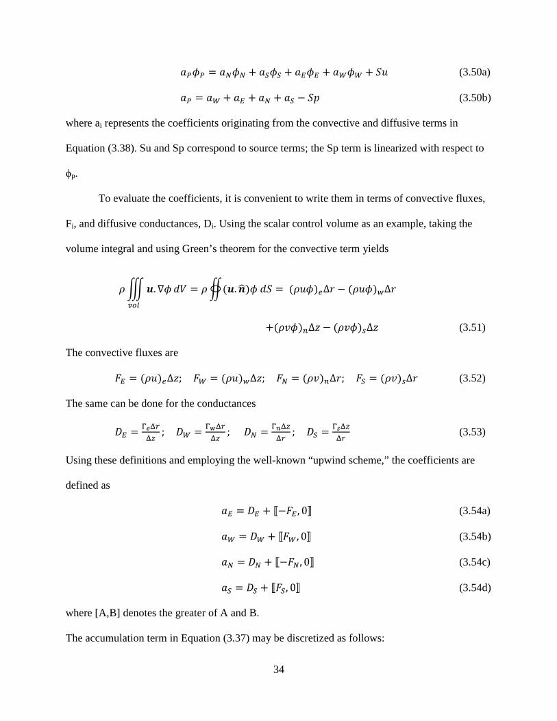
𝑎𝑃𝜙𝑃 = 𝑎𝑁𝜙𝑁 + 𝑎𝑆𝜙𝑆 + 𝑎𝐸𝜙𝐸 + 𝑎𝑊𝜙𝑊 + 𝑆𝑢 (3.50a)

𝑎𝑃 = 𝑎𝑊 + 𝑎𝐸 + 𝑎𝑁 + 𝑎𝑆 − 𝑆𝑝 (3.50b)

where ai represents the coefficients originating from the convective and diffusive terms in

Equation (3.38). Su and Sp correspond to source terms; the Sp term is linearized with respect to

ϕp.

To evaluate the coefficients, it is convenient to write them in terms of convective fluxes,

Fi, and diffusive conductances, Di. Using the scalar control volume as an example, taking the

volume integral and using Green’s theorem for the convective term yields

𝜌�𝒖.∇𝜙𝑣𝑜𝑙

𝑑𝑉 = 𝜌�(𝒖.𝒏�)𝜙 𝑑𝑆 = (𝜌𝑢𝜙)𝑒∆𝑟 − (𝜌𝑢𝜙)𝑤∆𝑟

+(𝜌𝑣𝜙)𝑛∆𝑧 − (𝜌𝑣𝜙)𝑠∆𝑧 (3.51)

The convective fluxes are

𝐹𝐸 = (𝜌𝑢)𝑒∆𝑧; 𝐹𝑊 = (𝜌𝑢)𝑤∆𝑧; 𝐹𝑁 = (𝜌𝑣)𝑛∆𝑟; 𝐹𝑆 = (𝜌𝑣)𝑠∆𝑟 (3.52)

The same can be done for the conductances

𝐷𝐸 = Γ𝑒Δ𝑟Δ𝑧

; 𝐷𝑊 = Γ𝑤Δ𝑟Δ𝑧

; 𝐷𝑁 = Γ𝑛Δ𝑧Δ𝑟

; 𝐷𝑆 = Γ𝑠Δ𝑧Δ𝑟

(3.53)

Using these definitions and employing the well-known “upwind scheme,” the coefficients are

defined as

𝑎𝐸 = 𝐷𝐸 + ⟦−𝐹𝐸 , 0⟧ (3.54a)

𝑎𝑊 = 𝐷𝑊 + ⟦𝐹𝑊 , 0⟧ (3.54b)

𝑎𝑁 = 𝐷𝑁 + ⟦−𝐹𝑁 , 0⟧ (3.54c)

𝑎𝑆 = 𝐷𝑆 + ⟦𝐹𝑆, 0⟧ (3.54d)

where [A,B] denotes the greater of A and B.

The accumulation term in Equation (3.37) may be discretized as follows:

35

𝜌∭ 𝜕𝜙𝜕𝑡

𝑑𝑉𝑣𝑜𝑙 = 𝜌(𝜙𝑃−𝜙𝑃∗ )

∆t∆𝑉 (3.55)

where ϕp* is the value of the variable at the previous time step. Since one term is linearized and

the other is not, the accumulation term may be split among Su and Sp as follows:

𝑆𝑢 = 𝜌𝜙𝑃∗∆𝑡−1∆𝑉; 𝑆𝑝 = −𝜌∆𝑡−1∆𝑉 (3.56)

Pertaining to the integrated form of Sϕ, the term may also be divided among the Su and Sp terms

in such a way that ensures the stability of the matrix solver. For a more in-depth discussion, see

Reference [54].

36

CHAPTER 4

RESULTS AND DISCUSSION

The model developed in Chapter 3 for describing the temperature and flow phenomena in

an electromagnetically stirred melt during solidification was used to investigate unidirectional

solidification of alloys in a bottom chill mold subjected to an axial magnetic field. This study

examines the variation of the velocity and turbulent characteristics, in both the bulk liquid and

mushy zone, with respect to solidification morphology. Emphasis will be placed on the influence

of grain size and solidification rate on the flow in the mushy region.

4.1 Description of the Model System

Figure 4.1 shows a sketch of the bottom chill mold used in this study. The mold consists

of an insulating refractory tube and a water-cooled stainless steel chill block. The chill block

allows water to flow through a cavity close to the top surface of the chill block, allowing for a

constant and uniform heat transfer coefficient at the chill block/metal interface. In this study, the

melt stirring is provided by a three-turn induction coil situated at one-half of the ingot height.

Due to the axial symmetry of the system, the electromagnetic field, fluid flow, and heat

transfer problems are two-dimensional, and the field equations need only to be calculated in the

r-z plane. The solution domain for the temperature, velocity, and turbulent fields consists of the

metal only, and is divided into a 30x30 non-uniform grid, shown in Figure 4.2. The boundary

conditions are also shown in this figure. For the electromagnetic field calculations, the solution

37

domain includes both the metal and the stainless steel chill block. In order to accurately describe

the exponential decay of the magnetic field in the metal due to the skin effect, a finer grid is used

near the outer radius.

Figure 4.1 Detailed Sketch of the Modeled System.

50 mm 40 mm

30 mm r

z

Al-4.5Cu (Specimen)

Refractory

Refractory

Stainless Steel (Chill Block)

40 m

m 70

mm

80 m

m

110

mm

120

mm

130

mm

16

0 m

m

Coil (3 turns)

Ø 8 mm

℄

65 mm

38

Figure 4.2 Gridded solution domain with boundary conditions

R

Z

0 0.01 0.02 0.03 0.040

0.02

0.04

0.06

0.08

𝜕𝑇𝜕𝑛

= 0,𝑢 = 0

𝑣 = 0, 𝑘 = 0,𝜕𝜀𝜕𝑛

= 0

𝑞 = ℎ(𝑇 − 𝑇∞), 𝑢 = 0

𝑣 = 0, 𝑘 = 0,𝜕𝜀𝜕𝑛

= 0

𝜕𝑇𝜕𝑛

= 0,𝑢 = 0 𝜕𝑣𝜕𝑛

= 0,𝜕𝑘𝜕𝑛

= 0,𝜕𝜀𝜕𝑛

= 0

𝜕𝑇𝜕𝑛

= 0,𝜕𝑢𝜕𝑛

= 0

𝑣 = 0,𝜕𝑘𝜕𝑛

= 0,𝜕𝜀𝜕𝑛

= 0

39

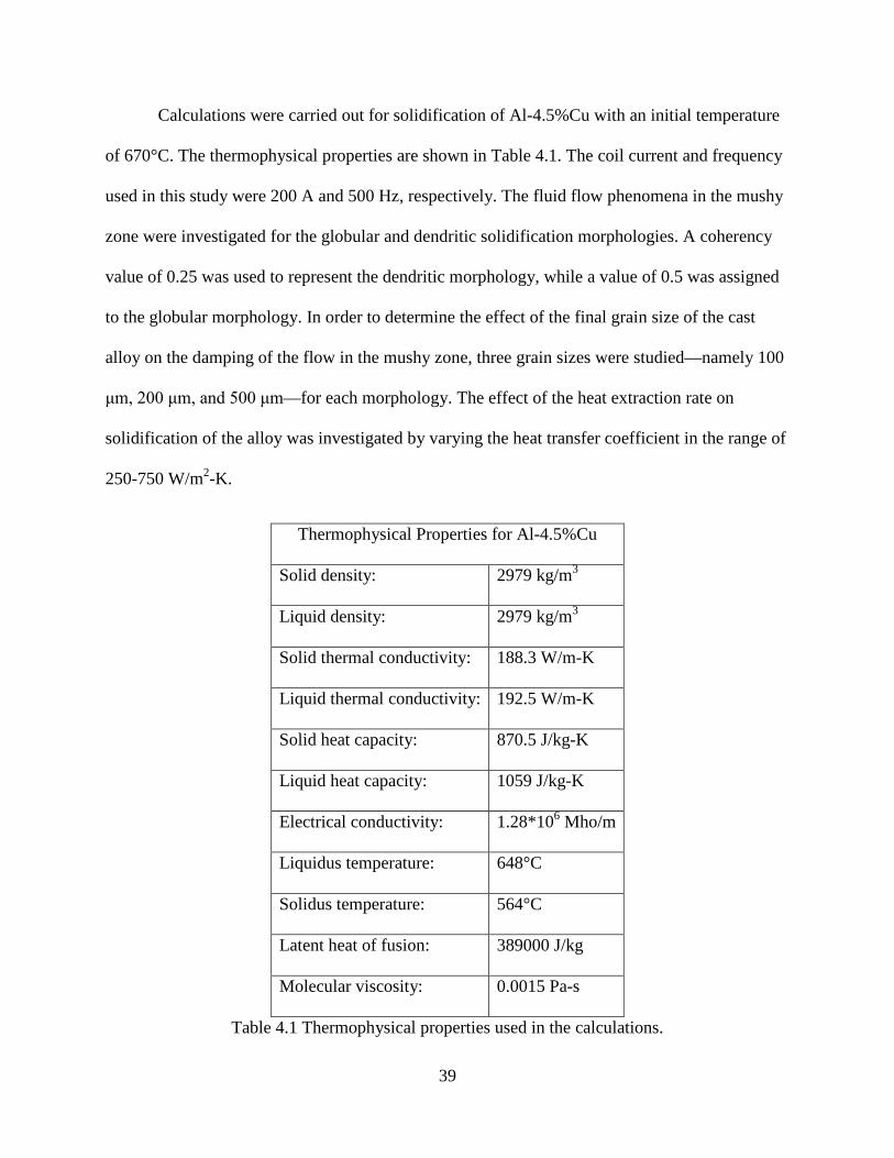
Calculations were carried out for solidification of Al-4.5%Cu with an initial temperature

of 670°C. The thermophysical properties are shown in Table 4.1. The coil current and frequency

used in this study were 200 A and 500 Hz, respectively. The fluid flow phenomena in the mushy

zone were investigated for the globular and dendritic solidification morphologies. A coherency

value of 0.25 was used to represent the dendritic morphology, while a value of 0.5 was assigned

to the globular morphology. In order to determine the effect of the final grain size of the cast

alloy on the damping of the flow in the mushy zone, three grain sizes were studied—namely 100

μm, 200 μm, and 500 μm—for each morphology. The effect of the heat extraction rate on

solidification of the alloy was investigated by varying the heat transfer coefficient in the range of

250-750 W/m2-K.

Thermophysical Properties for Al-4.5%Cu

Solid density: 2979 kg/m3

Liquid density: 2979 kg/m3

Solid thermal conductivity: 188.3 W/m-K

Liquid thermal conductivity: 192.5 W/m-K

Solid heat capacity: 870.5 J/kg-K

Liquid heat capacity: 1059 J/kg-K

Electrical conductivity: 1.28*106 Mho/m

Liquidus temperature: 648°C

Solidus temperature: 564°C

Latent heat of fusion: 389000 J/kg

Molecular viscosity: 0.0015 Pa-s

Table 4.1 Thermophysical properties used in the calculations.

40

4.2 Electromagnetic Field

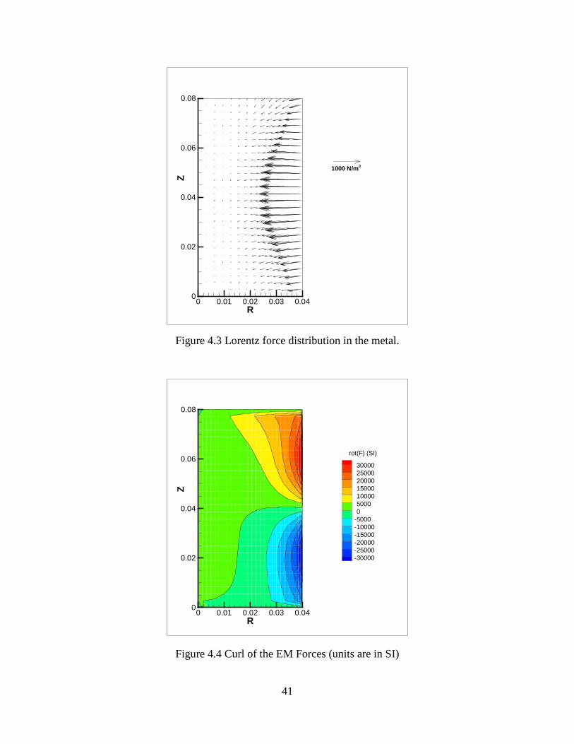
Figure 4.3 shows the computed electromagnetic (Lorentz) force field for a coil current of

200A and a frequency of 500 Hz. As expected, the forces exhibit positive divergence with

respect to the middle section of the ingot, which is expected since this point is coincident with

the axial midpoint of the coil. The maximum value of the Lorentz forces lies at the previously

mentioned point, with a magnitude of 104 N/m3, and the magnitude of the force expresses a

marked decrease along any given constant z plane as r tends less than R.

Of particular interest is the rotational component of the force, given by rot(Fem), which

drives the flow. This is shown in Figure 4.4. Upon inspection, one will easily notice that the

highest degrees of rotation occur at the outer radius at z=0.02 m and z=0.06 m, with opposite

signs, and that the curl of the field is zero at z=0.04 m. This means that the flow will feature two

axisymmetric recirculating loops, with the bottom loop rotating counterclockwise and the upper

loop rotating clockwise. The influence of the magnetic shields can also be seen in this figure. It

is observed that the magnitude of the curl is larger for z < 0.04 m. This is a result of the stronger

coupling of the magnetic field with the chill block relative to the metal, as the electrical

conductivity is higher for stainless steel than Al-4.5%Cu.

41

Figure 4.3 Lorentz force distribution in the metal.

Figure 4.4 Curl of the EM Forces (units are in SI)

R

Z

0 0.01 0.02 0.03 0.040

0.02

0.04

0.06

0.08

1000 N/m3

R

Z

0 0.01 0.02 0.03 0.040

0.02

0.04

0.06

0.08

rot(F) (SI)

300002500020000150001000050000

-5000-10000-15000-20000-25000-30000

42

Figure 4.5 shows the electrical energy dissipation in the metal. Like the electromagnetic

forces, the maximum values of Joule heating occur at the axial midpoint near the induction coil.

The maximum value of Joule heating was around 105 W/m3, and decreases for greater distance

from the field source. For the case investigated, the total heat generated in the metal was 13.5 W.

This quantity is much smaller than the rate of latent heat extraction from the melt, and therefore

the effect of Joule heating on the overall solidification rate is negligibly small. However, since

Joule heating acts to reduce the solidification rate, there will be some localized effect in regions

where Joule heating is relatively high (i.e. nearest the field source).

Figure 4.5 Joule heating in the metal (units are in SI)

R

Z

0 0.01 0.02 0.03 0.040

0.02

0.04

0.06

0.08

HS

100000900008000070000600005000040000300002000010000

43

4.3 Computed Results for Globular Solidification Morphology

4.3.1 Fluid Flow and Temperature Fields

(a) (b)

Figure 4.6 Velocity and temperature fields for (a) t=0; (b) t=30 s

Figures 4.6 and 4.7 show a typical evolution of the velocity and temperature fields—

presented in terms of solid fraction—during solidification for a grain size of 200 μm and heat

transfer coefficient of 500 W/m2-K. Figure 4.6a shows the velocity field prior to solidification

(t=0). As seen in this figure, the velocity field is characterized by two axisymmetric,

recirculating loops, which is expected for a stationary magnetic field. These two loops are

approximately the same size due to the positioning of the coil at the axial midpoint of the

specimen. It can also be seen that the characteristic velocity is approximately 20 mm/s. After 30s

(Figure 4.6b) the temperature at the base of the specimen has dropped below the liquidus

R

Z

0 0.01 0.02 0.03 0.040

0.02

0.04

0.06

0.08

f SOLID

10.90.80.70.60.50.40.30.20.10

TIME = .00 s

25 mm/s

R

Z

0 0.01 0.02 0.03 0.040

0.02

0.04

0.06

0.08

f SOLID

1.00.90.80.70.60.50.40.30.20.10.0

TIME = 30.00 s

25 mm/s

44

temperature, and the mushy zone now comprises approximately half of the height, causing

significant changes in the flow intensity in that region. However, it is clearly seen that the

maximum value of fs is less than the coherency value, fc, of 0.5. The solid fraction contours are

shown to align themselves tangentially with respect to the direction of the flow. This means that

convection is the dominant mode of heat transfer. It should also be observed that while the

magnitude of the velocity in the upper recirculating loop remains approximately the same as its

initial value, the velocity in the lower recirculating loop is sharply reduced by an order of

magnitude. This is a result of the damping force acting on the flow, the magnitude of which

increases with increasing solid fraction.

(a) (b)

Figure 4.7 Velocity and temperature fields for (a)t=60; (b) t=120 s

R

Z

0 0.01 0.02 0.03 0.040

0.02

0.04

0.06

0.08

f SOLID

10.90.80.70.60.50.40.30.20.10

TIME = 60.00 s

5 mm/s

R

Z

0 0.01 0.02 0.03 0.040

0.02

0.04

0.06

0.08

f SOLID

10.90.80.70.60.50.40.30.20.10

TIME =120.00 s

5 mm/s

45

Figure 4.7a shows the velocity and temperature fields after 60 seconds. At this

solidification time, the mushy zone now covers the entire domain, and the maximum value of

solid fraction is less than the coherency, meaning that solidification is still in the suspended

particle region. Note the change of the velocity scale for easier viewing. As seen in this figure,

the characteristic velocity in the upper loop is approximately 5 mm/s, and drops to less than 1

mm/s at the base of the metal, where solid fraction is close to coherency. These values are an

order of magnitude smaller than the velocity in the bulk liquid.

The flow in the fixed particle region is first shown in Figure 4.7b. This figure

corresponds to a solidification time of 120 seconds. As seen in this figure, the transition from the

suspended particle region to the fixed particle region is characterized by another significant drop

in the velocity. This is expected, as the formation of a stationary dendrite network provides

additional resistance to liquid phase motion via a reduction of the permeability in Darcian flow.

The significance of the decrease of the velocity is also observed in this figure. It can be seen that

the curvature of the isotherms at the mold wall decreases along with the velocity at higher solid

fraction, and the isosurface normal begins to align itself parallel to the heat flux. Thus it is clear

that the coherency point also marks the transition between convection-dominant heat transfer to

diffusion-dominant transfer.

46

(a) (b)

(c)

Figure 4.8 Velocity and temperature fields at later stages of solidification

R

Z

0 0.01 0.02 0.03 0.040

0.02

0.04

0.06

0.08

f SOLID

1.00.90.80.70.60.50.40.30.20.10.0

TIME =300.00 s

1 mm/s

RZ

0 0.01 0.02 0.03 0.040

0.02

0.04

0.06

0.08

f SOLID

1.00.90.80.70.60.50.40.30.20.10.0

TIME =360.00 s

1 mm/s

R

Z

0 0.01 0.02 0.03 0.040

0.02

0.04

0.06

0.08

f SOLID

1.00.90.80.70.60.50.40.30.20.10.0

TIME =420.00 s

1 mm/s

47

Figures 4.8(a-c) show the evolution of velocity and temperature fields at later stages of

solidification corresponding to 300, 360, and 420 seconds, respectively, where the solid fraction

is above the coherency value (fixed particle region). At t=300s, most of the metal is in the fixed

particle region, with only the top of the ingot remaining in the suspended particle region. It is

clear that heat transfer occurs via conduction. Observe that the flow only penetrates a few

millimeters into the fixed particle region, as the influence of Darcy damping is substantially

stronger than momentum transfer at the interface, in addition to the body forces being nil for fs <

fc. After 360 seconds, the fixed particle region now covers the entire domain. The velocity in this

region is now nil due to Darcy damping and the lack of any body forces to drive the flow in the

fixed particle region. Such is also the case for t=420s as well, where no fluid flow occurs and

heat transfer is by conduction only. This occurs until the end of solidification after 492 seconds.

Figure 4.9 presents a typical evolution of the turbulent kinetic energy for globular

solidification with grain size of 200 μm and a heat transfer coefficient of 500 W/m2-K. The

turbulence level in the bulk liquid is shown in Figure 4.9a. As seen in this figure, the turbulent

kinetic energy varies on the order of 10-3 J/kg near the centerline to 10-4 J/kg near the mold wall.

When compared to the fluid velocity, this suggests that the flow is highly turbulent in the bulk

liquid. In the initial stages of solidification, the turbulence level becomes highly attenuated in the

mushy region, as shown in Figure 4.9b. After 60s, it was found that turbulence was completely

dissipated.

48

(a) (b)

Figure 4.9 Turbulent kinetic energy profiles for (a) t=0s; (b) t=30s

4.3.2. Effect of Solidification Parameters

Figure 4.10 shows cooling curves for three different heat transfer coefficients

investigated, each taken at z/H=0.8 for a grain size of 200 μm. As seen in this figure, the

solidification times, defined by the time difference between the intersection of the cooling with

the solidus and liquidus lines, were determined to be 917, 453, and 301 seconds for heat transfer

coefficient values of 250, 500, and 750 W/m2-K, respectively. As expected, the solidification

time increases for decreasing h, reflecting the reduced heat extraction rate. There are three points

of inflection in each cooling curve. Starting from t=0, the first and last points of inflection are at

the liquidus and solidus temperatures, respectively. These correspond to the beginning and end

of latent heat evolution. The second point of inflection at the coherency is of particular interest,

R

Z

0 0.01 0.02 0.03 0.040

0.02

0.04

0.06

0.08

K

1.0E-039.0E-048.0E-047.0E-046.0E-045.0E-044.0E-043.0E-042.0E-041.0E-04

TIME= .00 SECONDS

RZ

0 0.01 0.02 0.03 0.040

0.02

0.04

0.06

0.08

K

1.0E-039.0E-048.0E-047.0E-046.0E-045.0E-044.0E-043.0E-042.0E-041.0E-04

TIME= 30.00 SECONDS

49

and corresponds to the previously mentioned transition in heat transfer modes from convection-

to diffusion-dominant.

Figure 4.10 Cooling curves for globular solidification at various h

Figure 4.11 gives the centerline velocity for z/H = 0.8 as a function of solid fraction for

three different grain sizes and a heat transfer coefficient of 500 W/m2-K. As seen in this figure,

there is a sharp decrease in the flow intensity in the initial stage of solidification (0<fs<0.1)

where the flow is damped by turbulent decay. This is expected, as damping is strongest in the

region of solid fraction 0<fs<0.05, where the particles are smallest and thus have the highest

surface-to-volume ratio. It is also seen that the intensity of the flow is stronger for increasing

final grain size. This stems from a smaller particle number density, which decreases the amount

of surface area where the Reynolds stresses can act. In terms of heat transfer, this means that

higher cooling rates for large-grained structures at the beginning of solidification.

TL: 648°C

Coherency: 606°C

TS: 564°C

TIME(s)

T(d

egC

)

0 200 400 600 800 1000 1200550

575

600

625

650

675

250 W/m2*K500 W/m2*K750 W/m2*K

50

As the solid fraction increases beyond a solid fraction of 0.1, the velocity remains nearly

constant, meaning very small changes in the rate of convective transfer. At fs~0.4, the flow

intensity decreases again until becoming almost negligible at the coherency point. Damping in

this region occurs due to a drop in the pressure gradient near the D’Arcy interface. The

additional damping also reduces the rate of heat transfer by convection to almost nil. As a result,

heat transfer for fs > 0.4 is primarily driven by conduction.

Figure 4.11 Velocity as a function of solid fraction for various Dg

Figure 4.12 shows a cooling curves for grain sizes of 100, 200, and 500 μm, with the heat

transfer coefficient of 500 W/m2-K. It can be clearly seen that the cooling rates for the fixed

particle region and the bulk liquid are nearly the same, but deviate within the suspended particle

region. Further inspection shows that the cooling rate is slightly higher for larger grain size. This

is consistent with the results shown in Figure 4.11, where the velocity was highest for large

grains and by corollary had the largest convective heat flux.

f

V(m

/s)

0 0.1 0.2 0.3 0.4 0.50

0.001

0.002

0.003

0.004

0.005

100 µm200 µm500 µm

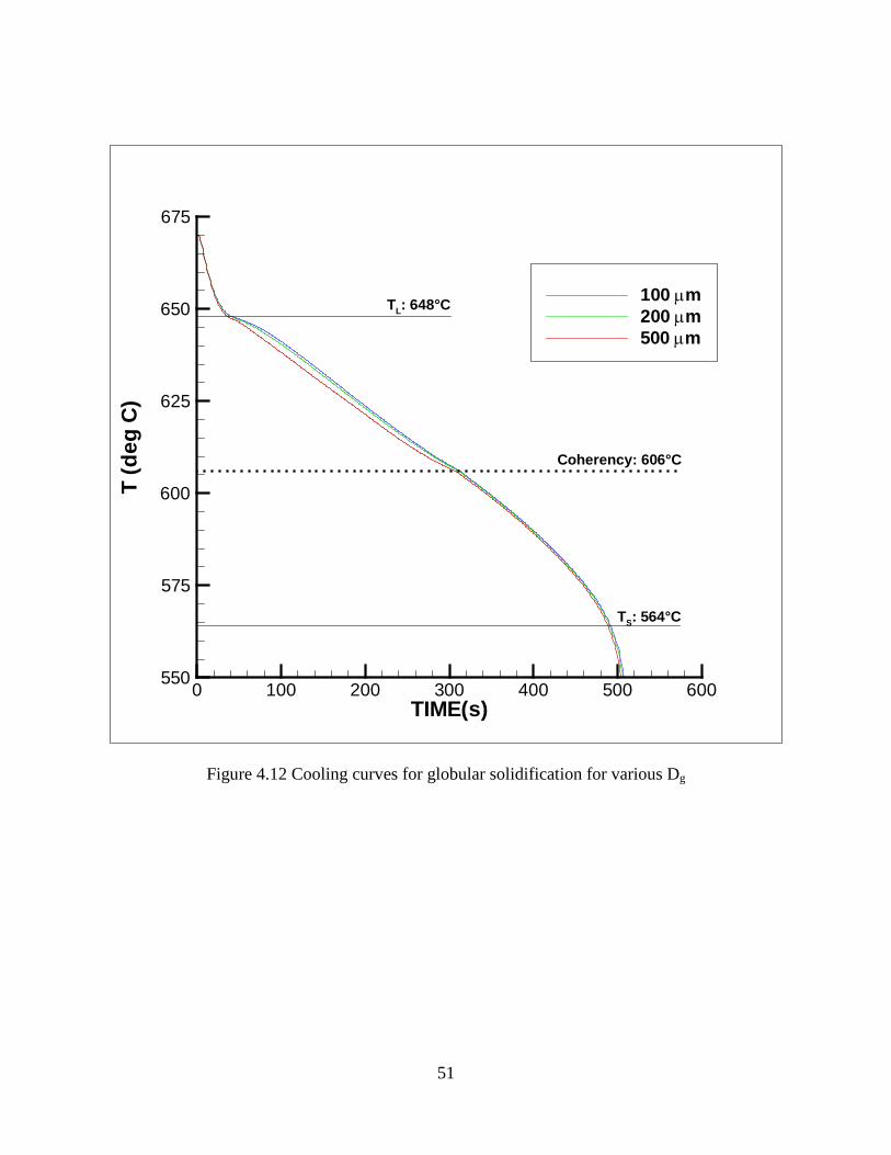
51

Figure 4.12 Cooling curves for globular solidification for various Dg

TIME(s)

T(d

egC

)

0 100 200 300 400 500 600550

575

600

625

650

675

100 µm200 µm500 µm

TL: 648°C

TS: 564°C

Coherency: 606°C

52

4.4 Computed Results for Dendritic Solidification Morphology

4.4.1 Fluid Flow and Temperature Profiles

Figure 4.13 shows the evolution of the velocity and temperature fields—the latter of

shown in terms of solid fraction—during solidification for a gain size of 200 μm and heat

transfer coefficient of 500 W/m2-K. As seen in Figure 4.13a, the velocity field prior to

solidification is identical to that of globular solidification in Figure 4.6a, which is expected. After

30 seconds, displayed in Figure 4.13b, the suspended particle region essentially covers the entire

bottom half of the ingot, similar to that of globular solidification, with the velocity being damped

by an order of magnitude. It should be said here that the magnitude of the velocity in the

suspended particle region is higher for dendritic solidification, for a given value of solid fraction.

The reason for this is the larger grain size given by Equation (3.47), which assumes the grain size

varies inversely with the coherency, allowing for higher velocities in this region.

The most important contribution of the coherency may be seen in Figure 4.13c, which

shows the velocity and temperature field after 60 seconds. It can be seen here that the fixed

particle region first appears, shown by the additional isotherm for better clarity. Like its globular

counterpart, there is a significant decrease of the velocity—approximately an order of

magnitude—in the fixed particle region due to Darcy damping. However, it is important to note

that there is greater penetration of fluid into the fixed particle region for dendritic solidification

than globular solidification due to higher permeability of dendritic structures at the coherency

point. The lower value of coherency also signals an earlier transition to conduction-dominant

heat transfer from convection-dominant.

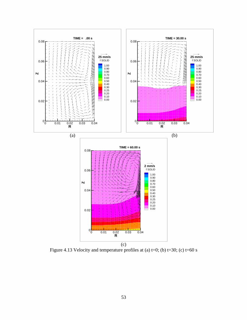
53

(a) (b)

(c)

Figure 4.13 Velocity and temperature profiles at (a) t=0; (b) t=30; (c) t=60 s

R

Z

0 0.01 0.02 0.03 0.040

0.02

0.04

0.06

0.08

f SOLID

1.000.900.800.700.600.500.400.300.250.200.100.00

TIME = .00 s

25 mm/s

RZ

0 0.01 0.02 0.03 0.040

0.02

0.04

0.06

0.08

f SOLID

1.000.900.800.700.600.500.400.300.250.200.100.00

TIME = 30.00 s

25 mm/s

R

Z

0 0.01 0.02 0.03 0.040

0.02

0.04

0.06

0.08

f SOLID

1.000.900.800.700.600.500.400.300.250.200.100.00

TIME = 60.00 s

2 mm/s

54

Figure 4.14 shows the evolution of the temperature and velocity fields at later stages of

solidification. After 120 seconds (Figure 4.14a), the fixed particle region occupies the bottom

third of the metal. The increased penetration depth of the flow can also be better observed in this

figure, as it can be seen that the velocity just beyond the coherency isotherm is approximately 1

mm/s and is on the order of 0.3 mm/s at fs~0.3. This may be contrasted with the characteristic

velocity 0.1 mm/s at fc for globular solidification. It was also found that the velocity becomes nil

for fs ≥ 0.4. Furthermore, the isotherms in dendritic solidification are relatively in the same

position as those of globular solidification, but that the curvature of each isotherm in the fixed

particle region is more planar for dendritic solidification, as conduction becomes the primary

means of heat transfer more quickly. As the solidification continues in the proceeding figures

(t≥240s), the velocity continues to be nil throughout the metal, similar to globular solidification,

until the metal completely solidifies after 504 seconds.

Figure 4.15 shows the evolution of the turbulent kinetic energy during solidification for

the case described by Figures 4.13 and 4.14. As expected, the values of the turbulent kinetic

energy prior to solidification are the same as those of the globular cases. It is also clear that the

turbulence levels continue to mimic those of globular solidification as solidification progresses.

This suggests that the value of coherency has no effect on the damping of turbulent kinetic

energy, as it occurs at values of solid fraction well below fc.

55

(a) (b)

(c) (d)

Figure 4.14 Velocity and temperature profiles at

(a) t=120; (b) t=240; (c) t=300; (d) t=480 s

R

Z

0 0.01 0.02 0.03 0.040

0.02

0.04

0.06

0.08

f SOLID

1.000.900.800.700.600.500.400.300.250.200.100.00

TIME =120.00 s

2 mm/s

RZ

0 0.01 0.02 0.03 0.040

0.02

0.04

0.06

0.08

f SOLID

1.000.900.800.700.600.500.400.300.250.200.100.00

TIME =240.00 s

2 mm/s

R

Z

0 0.01 0.02 0.03 0.040

0.02

0.04

0.06

0.08

f SOLID

1.000.900.800.700.600.500.400.300.250.200.100.00

TIME =300.00 s

2 mm/s

R

Z

0 0.01 0.02 0.03 0.040

0.02

0.04

0.06

0.08

f SOLID

1.000.900.800.700.600.500.400.300.250.200.100.00

TIME =480.01 s

2 mm/s

56

(a) (b)

Figure 4.15 Turbulent kinetic energy profiles at (a) t=0; (b) t=30 s

4.4.2 Effect of Solidification Parameters

Figure 4.16 shows the influence of heat transfer coefficient on solidification of an alloy

exhibiting a dendritic morphology. Each cooling curve in this figure was taken at z/H=0.8 and a

final grain size of 200 μm. It can immediately be seen that the seconds point of inflection has

shifted to T=627°C, which corresponds to an fs of 0.25 (i.e. the coherency point). It is also found

that the solidification times are 929, 455, and 311 seconds for heat transfer coefficient values of

250, 500, and 750 W/m2-K, respectively. As expected, the solidification times for dendritic

morphology are very close to those of globular morphology, as the heat generation and

extraction rates are identical given the fact that electrical energy dissipation in the metal is

negligible. Figure 4.17 further illustrates the similarity between the globular and dendritic

solidification times by plotting them with respect to the Biot number (Bi=hL/ks).

R

Z

0 0.01 0.02 0.03 0.040

0.02

0.04

0.06

0.08

K

1.0E-039.0E-048.0E-047.0E-046.0E-045.0E-044.0E-043.0E-042.0E-041.0E-04

TIME= .00 SECONDS

RZ

0 0.01 0.02 0.03 0.040

0.02

0.04

0.06

0.08

K

1.0E-039.0E-048.0E-047.0E-046.0E-045.0E-044.0E-043.0E-042.0E-041.0E-04

TIME= 30.00 SECONDS

57

Figure 4.16 Cooling curves for dendritic solidification with variable h

Figure 4.17 Influence of heat transfer coefficient on solidification time

TIME(s)

T(d

egC

)

0 200 400 600 800 1000 1200550

575

600

625

650

675

250 W/m2-K500 W/m2-K750 W/m2-K

TS: 564°C

Tcoh: 627°C

TL: 648°C

58

Figure 4.18 shows the influence of the final grain size on the centerline velocity at

z/H=0.8. In this figure, it can be clearly seen that the relationship between grain size and velocity

for globular solidification (see Figure 4.11) is maintained for dendritic morphology. However, it

should be noted that the centerline velocity values are higher for the dendritic morphology, in

additional to the lower initial decay rate. This is a result of the more rapid grain growth rate for

the dendritic morphology, as it was assumed that the grain size was inversely related to the

coherency solid fraction, resulting in lower damping force acting on the fluid in the initial stages

of solidification.

Figure 4.18 Centerline velocity for dendritic morphology for various Dg

f

V(m

/s)

0 0.05 0.1 0.15 0.2 0.250

0.002

0.004

0.006

0.008

100 µm200 µm500 µm

59

Figure 4.19 Cooling curves for three different Dg with dendritic morphology

Figure 4.19 shows three cooling curves for the three grain sizes investigated at the

centerline for z/H=0.8. In general, it can again be seen that the temperature evolution, for both

dendritic and globular morphologies, is nearly the same, and that the relationship between the

cooling rate and grain size in the suspended particle region continues to hold. It is important to

note that unlike the globular cooling curves, there is some noticeable deviation in the cooling

curves past the coherency point. This is caused by the increased penetration depth of the flow

Tcoh: 627°C

TS: 564°C

TL: 648°C

TIME(s)

T(d

egC

)

0 150 300 450 600550

575

600

625

650

675100 µm200 µm500 µm

60

into the fixed particle region, making convection still the preeminent mode of heat transfer. This

deviation becomes unnoticeable by fs~0.3 (~620°C), since Darcy damping is significant enough

to make the Peclet number—the ratio of convective and diffusive heat transfer—small. The

solidification times for each grain size were found to be less than one percent from one another.

61

CHAPTER 5

CONCLUDING REMARKS AND RECOMMENDATIONS

5.1 Concluding Remarks

1. A model has been developed to describe the electromagnetic and fluid flow phenomena

in an EM stirred melt during solidification

2. Flow in the mushy zone was described by dividing it into two regions: The fixed particle

region and the suspended particle region. The boundary between these two regions was

defined by the coherency solid fraction.

3. Damping of the flow in the suspended particle region occurs through interaction of the

turbulent stresses with the crystallite surfaces, while the flow was damped in the fixed

particle region by Darcy’s law.

4. Calculations were carried out for solidification of the Al-4.5%Cu alloy in a bottom chill

mold undergoing linear stirring.

5. It was found that the velocity damping takes place in the initial stages of solidification

(fs<0.1), and the velocity in the suspended particle region was an order of magnitude

smaller than that of the bulk liquid.

6. The strength of the damping force was lessened with both larger grain size and small

values of coherency solid fraction.

62

7. Turbulence levels are similarly damped at very low solid fraction, and were found to be

negligible after fs~0.1.

8. Darcian behavior in the fixed particle region further reduced the velocity, with the fluid

reaching negligible values a few millimeters below the coherency isotherm. The

penetration depth of the flow was shown to increase with lower coherency values.

9. The values of coherency solid fraction and final grain size were shown to have minimal

effect on the overall solidification time.

10. The coherency point tends to demarcate the region of solid fraction where the primary

mode of heat transfer transitions from convection to conduction.

11. Although the overall solidification rate was unchanged by the coherency value or final

grain size, there is local effect on the flow with respect to the suspended particle region.

The cooling rate in the initial stages of solidification was shown to increase for larger

grain size.

5.2 Recommendations for Future Research

1. Determine the effect of coil geometry, coil current, and coil frequency on the flow

structure and intensity in the mushy zone during solidification.

2. Perform experiments to validate the model developed in this work.

3. Expand the model to include mass transfer of the alloying elements to determine predict

macro/microsegregation in the final casting.

4. Investigate the effect of coil geometry, coil current, and coil frequency on the evolution

of the flow during solidification.

5. Determine the effect of electromagnetic stirring on macro/microsegregation of the cast

alloy.

63

REFERENCES

(1) N El-Kaddah, J Szekely. The turbulent recirculating flow in a coreless induction furnace, a comparison of theoretical predictions with measurements. J. Fluid Mechanics 133(1983), 33-46. (2) AA Tzavaras, HD Brody. Electromagnetic stirring and continuous casting— Achievements, problems, and goals. JOM 36(3)(1984), 31-37. (3) C Vives. New electromagnetic rheocasters for the production of thixotropic aluminum alloy systems. in Magnetohydrodynamics in Process Metallurgy. eds. J Szekely, JW Evans, K Blazek, N El-Kaddah (Warrendale: TMS, 1991), 169-174. (4) VA Kompan, et al. Magnetically controlled electroslag melting of titanium alloys. in Modeling for Materials Processing, (Riga, 2010), 85-90. (5) C Vives, C Perry. Effect of electromagnetic stirring during the controlled solidification of tin. Int. J. Heat Mass Transfer 29(1986), 21-33. (6) L Hachani, et al. Experimental analysis of the solidification of Sn-3wt%Pb alloy under natural convection. Int. J. Heat Mass Transfer 55(2012), 1986-1996. (7) Q Zhao, et al. The effects of electromagnetic stirring on the solidification structure and macrosegregation of Pb-Sn alloy. Adv. Mater. Res. 484(2012), 1447-1452. (8) JA Burton, RC Prim, WP Schlicter. The distribution of solute in crystals grown from the melt—Part I: Theoretical. J. Chem. Phys. 21(1953), 1987-1991. (9) T Takahashi, K Ichikawa, M Kudou. Effect of fluid flow on macrosegregation in steel ingots. Trans ISIJ, 16(1976), 283-291. (10) B Wang, Y Yang, W Tang. Microstructure refinement of AZ91D alloy solidified with pulsed magnetic field. Trans. Nonferrous Met. Soc. China 18(2008), 536-540. (11) B Chalmers. Principles of Solidification. (New York: Wiley, 1964) (12) WC Winegard, B Chalmers. Supercooling and dendritic freezing in alloys. Trans. Amer. Soc. Metals, 46(1953), 1214-1224. (13) Q Han, A Hellawell. Primary particle melting rates and equiaxed grain nucleation. Met. Mater. Trans. B, 28(1997), 169-173. (14) B Chalmers. The structure of ingots. J. Aust. Inst Metals 8(1963), 255-263.

64

(15) B Willers, et al. The columnar-to-equiaxed transition in Pb-Sn alloys affected by electromagnetically driven convection. Mat Sci Eng A 402(2005), 55-65. (16) KA Jackson, JD Hunt, DR Uhlmann, TP Seward III. On the origin of the equiaxed zone in castings. Trans Met Soc AIME, 236 (1966), 149-158. (17) CJ Parides, RN Smith, ME Glicksman. The influence of convection during solidification on fragmentation of the mushy zone of a model alloy. Met. Trans. A 28(1997), 875-883. (18) B Li, HD Brody, A Kazimirov. Real-time observation of dendrite coarsening in Sn- 13wt%Bi alloys by synchrotron microradiography. Phys. Rev. E 70(2004), 062602. (19) D Ruvalcaba, et al. In-situ observation of dendrite fragmentation due to local solute- enrichment during directional solidification of an aluminum alloy. Acta. Mater. 55(2007), 4287-4292. (20) JA Dantzig, M Rappaz. Solidification. (Lausanne: EPFL Press, 2009).464-466. (21) J Szekely. The role of software in mathematical modeling. in Materials Processing in the Computer Age. eds. VR Voller, MS Stacjpwocz. BG Thomas. (Warrendale: TMS, 1991), 21-34. (22) SD Ridder, et al. Steady state segregation and heat flow in ESR. Met. Trans. B 9(1978), 415-425. (23) SD Riddler, S Kou, R Mehrabian. Effect of fluid flow on macrosegregation in axisymmetric ingots. Met. Trans. B 12(1981), 435-447. (24) VR Voller, C Prakash. A fixed grid numerical modeling methodology for convection- diffusion mushy region phase-change problems. Int. J. Heat Mass Transfer 30(1987), 1709-1719. (25) WD Bennon, FP Incropera. A continuum model for momentum, heat, and species transport in binary solid-liquid phase change systems—I: Model formulation. Int. J. Heat Mass Transfer 30(1987), 2161-2170. (26) T Campanella, C Charbon, M Rappaz. Influence of permeability on the grain refinement induced by forced convection in copper-base alloys. Scripta Mater. 49(2003), 1029- 1034. (27) PC Carman. Fluid flow through granular beds. Trans. Inst. Chem. Eng. 15(1937), 150- 166. (28) DR Poirier. Permeability for flow of interdendritic liquid in columnar-dendritic alloys. Met. Trans. B 18(1987), 245-255.

65

(29) W Shyy, et al. Modeling of turbulent transport and solidification during continuous ingot casting. Int. J. Heat Mass Transfer 35(1992), 1229-1245. (30) PJ Prescott, FP Incropera. The effect of turbulence on solidification of a binary metal alloy with electromagnetic stirring. J. Heat Transfer 117(1995), 716-724. (31) Budenkova, et al. Simulation of a directional solidification of a binary Al-7wt%Si and a ternary alloy Al-7wt%Si-1wt%Fe under the action of a rotating magnetic field. Proc. MCWASP XIII, IOP Conference Series: Mat. Sci. Eng. 33(2012), 012046. (32) D Apelian, MC Flemings, R Mehrabian. Specific permeability of partially solidified dendritic networks of Al-Si alloys. Met. Trans. 5(1974), 2533-2537. (33) N Streat, F Weinberg. Interdendritic fluid flow in a lead-tin alloy. Met. Trans. B 7(1976), 417-423. (34) R Nasser-Rafi, R Deshmukh, DR Poirier. Flow of interdendritic liquid and permeability in Pb-20wt%Sn alloys. Met. Mater. Trans. A 16(1985), 2263-2271. (35) CM Oldenburg, FJ Spera. Hybrid model for solidification and convection. Num. Heat Transfer B 21(1992), 217-229. (36) CY Wang, S Ahuja, C Beckermann, HC de Groh III. Multiparticle interfacial drag in equiaxed solidification. Met. Trans. B 26(1995), 111-119. (37) J Ni, C Beckermann. A volume-averaged two-phase model for transport phenomena during solidification. Met. Trans. B 22(1991), 349-361 (38) J Ni, FP Incropera. Extension of the continuum model for transport phenomena occurring during metal alloy solidification—II: Microscopic considerations. Int. J. Heat Mass Transfer 38(1995), 1285-1296. (39) PA Nikrityuk, K Eckert, R Grundmann. A numerical study of unidirectional solidification of a binary metal alloy under influence of a rotating magnetic field. Int J Heat Mass Transfer 49(2006), 1501-1515. (40) R Pardeshi, AK Singh, P Dutta. Modeling of solidification process in a rotary electromagnetic stirrer. Num. Heat Transfer A 55(2008), 42-57. (41) JD Jackson. Classical Electrodynamics, 3rd Edition. (New York: Wiley, 1999). (42) D Roger, JF Eastham. Finite element solution of 3D eddy current flow in magnetically linear conductors at power frequencies. IEEE Trans. Magn. 18(1982), 481-485.

66

(43) RD Pillsbury. A three dimensional eddy current formulation using two potentials: The magnetic vector potential and total scalar potential. IEEE Trans. Magn. 19(1983), 2284- 2287. (44) D Roger, JF Eastham. Multiply connected regions in the A-Y three-dimensional eddy current formulation. Proc. IEE 134(1987), 58-66. (45) MVK Chari, A Konrad, MA Palmo, J D’Angelo. Three dimensional vector potential analysis for machine field problems. IEEE Trans. Magn. 18(1982), 436-446. (46) CS Biddlecombe, EA Heighway, J Simkin, CW Trowbridge. Methods for eddy current computation in three dimensions. IEEE Trans. Magn. 18(1982), 492-497. (47) CJ Carpenter. Comparison of alternative formulations of 3-dimensional magnetic field and eddy-current problems at power frequencies. Proc. IEE 124(1977), 1026-1034. (48) CJ Carpenter, EA Wyatt. Efficiency of numerical techniques for computing eddy currents in two and three dimensions. Proc COMPUMAG-76 (1976), 242-250. (49) CJ Carpenter, DH Locke. Numerical models of three-dimensional end winding arrays. Proc. COMPUMAG-76 (1976), 47-55. (50) TW Preston, ABJ Reese. Solution of 3-dimensional eddy current problems: The T-Ω method. IEEE Trans. Magn. 18(1982), 486-491. (51) W Reinhart, H Stogner, K Pries. Calculation of 3D eddy current problems by finite element method using either an electric or magnetic vector potential. IEEE Trans. Magn. 24(1988), 122-125. (52) Biro, K Pries. Finite element analysis of 3D eddy currents. IEEE Trans. Magn. 26(1990), 418-423. (53) JN Reddy. An Introduction to the Finite Element Method. (New York: McGraw-Hill, 1993). (54) SV Patankar. Numerical Heat Transfer and Fluid Flow. (New York: McGraw-Hill, 1980). (55) GD Smith. Numerical Solution of Partial Differential Equations. (New York: Oxford University Press, 1965). (56) SJ Salon. The hybrid finite element-boundary element method in electromagnetics. IEEE Trans. Magn. 21(1985), 1829-1834. (57) JL Meyer, N El-Kaddah, J Szekely. A new method for computing electromagnetic force fields in induction furnace. IEEE Trans. Magn. 23(1987), 1806-1810.

67

(58) TT Natarajan, N El-Kaddah. A finite element-integral method for two-dimensional eddy current problems. in Magnetohydrodynamics in Process Metallurgy. eds J Szekely, JW Evans, K Blazek, N El-Kaddah. (Warrendale, PA: TMS, 1991). 3-9. (59) TT Natarajan. An efficient two dimensional FEM/integral method for electromagnetic problems. MS Thesis, University of Alabama, 1991. (60) E Kolbe, W Reiss. Eine method zur numerische bestimmung der stromdichteverteilung in inductive erwarmten korpen unterschiedlicher geometrisher form. Wiss. Z der TH Ilmenau 9(1963), 311-317. (61) RF Dudley, PE Burke. The prediction of current distribution in induction heating installations. IEEE Trans. Industry Applications 8(1972), 565-571. (62) FW Grover. Inductance Calculations. (New York: D Van Nostrand, 1946). (63) JD Lavers. The influence of system geometry on the electromagnetic stirring forces in crucible induction melting furnaces. in Metallurgical Applications of Magnetohydrodynamics. eds HK Moffat, MRE Proctor. (London: The Metals Society, 1984), 62-77. (64) JL Meyer, J Szekely, N El-Kaddah. Calculation of the electromagnetic field for induction stirring in continuous casting. ISIJ Intl. 27(1987), 25-33. (65) JD Lavers. Computational methods for the analysis of molten metal electromagnetic confinement systems. ISIJ Intl. 29(1989), 993-1005. (66) ERG Eckert, RM Drake. Analysis of Heat and Mass Transfer. (New York: McGraw-Hill, 1972). (67) FC Frank. Radially symmetric phase growth controlled by diffusion. Proc. Roy. Soc. A 201(1950), 586-599. (68) S Paterson. Propagation of a boundary of fusion. Proc Glasgow Math Assoc 1(1952), 42- 47. (69) PL Chambre. On the dynamics of phase growth. Quart. J. Mech. Appl. Math. 9(1956), 224-233. (70) TR Goodman. The heat balance integral and its application to problems involving a change in phase. Trans ASME 8(1958), 335-342. (71) NMH Lightfoot. The solidification of steel ingots. Proc. London Math. Soc. 31(1929), 97-116.

68

(72) KA Rathjen, LM Jiji. Heat conduction with melting or freezing in a moving corner. J Heat Transfer 93(1971), 101-109. (73) H Budhia, F Krieth. Heat transfer with melting or freezing in a wedge. Int J Heat Mass Transfer 16(1973), 195-211. (74) LI Rubinstein. The Stefan Problem. (Providence: American Mathematical Society, 1971). (75) WD Murray, F Landis. Numerical and machine solutions of transient heat-conduction problems involving melting or freezing. J Heat Transfer 81(1959), 106-112. (76) SO Unverdi, G Tryggvason. A front-tracking method for viscous, incompressible, multi- fluid flows. J Comp Phys 100(1992), 25-37. (77) S Osher, JA Sethian. Fronts propagating with curvature-dependent speed: Algorithms based on Hamilton-Jacobi formulations. J. Comp. Phys. 79(1988), 12-49. (78) J Crank. Two methods for the numerical solution of moving-boundary problems in diffusion and heat flow. Quart J Mech Appl Math 10(1957), 220-231. (79) JL Duda, MF Malone, RH Notter, JS Vrentas. Analysis of two-dimensional diffusion- controlled moving boundary problems. Int J Heat Mass Transfer 18(1975), 901-910. (80) T Saitoh. Numerical method for multi-dimensional freezing problems in arbitrary domains. J Heat Transfer 100(1978), 294-299. (81) CF Hsu, EM Sparrow, SV Patankar. Numerical solution of moving boundary problems by boundary immobilization and a control-volume-based finite-difference scheme. Int J Heat Mass Transfer 24(1981), 1335-1343. (82) M Lacroix, VR Voller. Finite difference solutions of solidification phase change problems: Transformed grids versus fixed grids. Num Heat Transfer B 17(1990), 25-41. (83) AN Thionov, AA Samarskii. The Equations of Mathematical Physics, 2nd Ed. (Moscow: Gittl, 1953). (84) J Szekely, NJ Thelemis. Rate Phenomena in Process Metallurgy. (New York: Wiley, 1971). (85) BM Budak, EN Sobol’eva, AB Uspenskii. A difference method with coefficient smoothing for the solution of Stefan problems. Zh Vychisl Mat Mat Fiz (5)(1965), 828- 840. (86) AA Samarskii, BD Moisynko. An economic continuous calculation scheme for the Stefan multidimensional problem. Zh Vychisl Mat Mat Fiz (5)(1965), 816-827.

69

(87) DM Stefanescu. Science and Engineering of Casting Solidification, 2nd Ed. (New York: Springer, 2009). pp. 97-99. (88) G Poole, N Rimkus, A Murphy, P Boehmcke, N El-Kaddah. Effect of the solidification rate on microstructure of cast Mg alloys at low superheat. in Magnesium Technology 2012. eds. SN Mathaudhu, WH Sillekens, NR Neelameggham, N Hort (Warrendale: TMS, 2012), 161-164. (89) DGR Sharma, M Krishnan, C Ravindran. Determination of the rate of latent heat liberation in binary alloys. Mater Characterization 44(2000), 309-320. (90) CA Siqueira, N Cheung, A Garcia. The columnar to equiaxed transition during solidification of Sn-Pb alloys. J Alloys and Compounds 351(2003), 126-134. (91) KD Carlson, C Beckermann. Determination of solid fraction-temperature relation and latent heat using full scale casting experiments: application to corrosion resistant steels and nickel based alloys. Int J Cast Metals Research 25(2012), 75-92. (92) Y Li, D Apelian, B Xing, Y Ma, Y Hao. Commerical AM60 alloy for semisolid processing: Alloy optimization and thermodynamic analysis. Trans Nonferrous Metals Soc China. 20(2010), 1572-1578. (93) R Trivedi, S Liu, P Mazumder, E Simsek. Microstructure development in directionally solidified Al-4.0wt%Cu alloy system. Sci Tech Adv Mater 2(2001), 309-320. (94) SA Thorpe, PK Hutt, R Soulsby. The effect of horizontal gradients on thermohaline convection. J Fluid Mech 38(1969), 375-400. (95) JE Hart. On sideways diffusive instability. J Fluid Mech 99(1971), 279-288. (96) CF Chen. Onset of cellular convection in a salinity gradient due to a lateral temperature gradient. J. Fluid Mech. 63(1974), 563-576. (97) ME Thompson, J Szekely. Mathematical and physical modeling of double-diffusive convection of aqueous solutions crystallizing at a vertical wall. J Fluid Mech 187(1988), 409-433. (98) HE Huppert, MG Worster. Dynamic solidification of a binary melt. Nature 314(1985), 367-384. (99) MG Worster. Solidification of an alloy from cooled boundary. J Fluid Mech 167(1986), 481-501. (100) W Kurz, DJ Fisher. Fundamentals of Solidification. (Rockport, MA: Trans Tech Publications, 1986), 91.

70

(101) MJ Stewart. Natural Convection in Liquid Metals. PhD Dissertation, University of British Columbia, 1970. (102) D Brabazon, DJ Browne, AJ Carr. Mechanical stir casting of aluminum alloys from the mushy state: Process, microstructure, and mechanical properties. Mater Sci Eng A 326(2002), 370-381. (103) H Puga. JC Teixeira, J Barbosa, E Seabra, S Ribeiro, M Prokic. The combined effect of melt stirring and ultrasonic agitation on the degassing efficiency of AlSi9Cu3 alloy. Mater Lett 63(2009), 2089-2092. (104) SF Liu, LY Liu, LG Kang. Refinement role of electromagnetic stirring and strontium in AZ91 magnesium alloy. J. Alloys Compounds 450(2008) 546-550. (105) AV Kuznetsov. Investigation of the coupled heat transfer, fluid flow, and the solute transport during the strip casting process. Int J Heat Mass Transfer 40(1997), 2949-2961. (106) TS Piwonka, MC Flemings. Pore formation in solidification. Trans Met Soc AIME 236(1966), 1157-1165. (107) R Mehrabian, M Keane, MC Flemings. Interdendritic fluid flow and macrosegregation: Influence of gravity. Met. Trans. 1(1970), 1209-1219. (108) R Mehrabian, M Keane, MC Flemings. Macrosegregation in ternary alloys. Met Trans 1(1970), 455-464. (109) J Szekely, AS Jassal. An experimental and analytical study of the solidification of a binary dendritic system. Met. Trans. B 9(1978), 389-397. (110) S Ganesan, CL Chan, DR Poirier. Permeability for flow parallel to primary dendrite arms. Mater. Sci. Eng. A 151(1992), 97-105. (111) RB Bird, WE Stewart, EN Lightfoot. Transport Phenomena. (New York: Wiley, 1960), pp 196-200. (112) S Kou, DR Poirier, MC Flemings. Macrosegregation in rotated remelted ingots. Met. Trans. B 9(1978), 711-719. (113) S Felicelli, JC Heinrich, DR Poirier. Simulation of freckles during vertical solidification of binary alloys. Met. Trans. B 22(1991) 847-859. (114) AL Maples, DR Poirier. Convection in the two-phase zone of solidifying alloys. Met. Trans. B 15(1984), 163-172. (115) K Murakami, A Shiraishi, T Okamoto. Interdendritic fluid flow normal to primary dendrite arms in cubic alloys, Acta Metall. 31(1983), 1417-1424.

71

(116) K Murakami, T Okamoto. Fluid flow in interdendritic space in cubic alloys. Acta Metall 32(1984), 1423-1428 (117) RG Santos, MLNM Melo. Permeability of interdendritic channels. Mater. Sci. Eng. A 391(2005), 151-158. (118) HC de Groh III, PD Weidman, R Zakhem, S Ahuja, C Beckermann. Calculation of a dendrite settling velocities using a porous envelope. Met Trans B 24(1993), 749-753.\ (119) H Danon, M Wolfshtein, G Hetsroni. Numerical calculations of two-phase turbulent round jet. Int. J. Multiphase Flow 3(1977), 223-234. (120) WP Jones, BE Launder. The prediction of laminarization with a two-equation model of turbulence. Int. J. Heat Mass Transfer 15(1972), 301-314. (121) H Tennekes, JL Lumley. A First Course in Turbulence. (Cambridge, MA: MIT Press, 1972). (122) R West. On the permeability of the two-phase zone during solidification of alloys. Met. Trans. A 16(1985), 693. (123) S Chang, DM Stefanescu. A model for macrosegregation and its application to Al-Cu castings. Met. Trans. A 27(1996), 2708-2721. (124) OJ Ilegbusi, MD Mat. Modeling flowability of the mushy zone with a hybrid model utilizing coherency solid fraction. Mater. Sci. Eng. A 247(1998), 135-141. (125) MD Mat, OJ Ilegbusi. Application of a hybrid model of mushy zone to macrosegregation in alloy solidification. Int. J. Heat Mass Transfer 45(2002), 279-289. (126) BE Launder, DB Spalding. Mathematical Models of Turbulence. (London, Academic Press, 1972). (127) M Mooney. The viscosity of a concentrated suspension of spherical particles. J Colloid

Science 6(1951), 162-170.