modeling of foundation heat exchangers · modeling of foundation heat exchangers is similar to...

P128,

8th International Conference on System Simulation in Buildings, Liege, December 13-15, 2010

Modeling of Foundation Heat Exchangers

L. Xing1*, J. D. Spitler1, J. R. Cullin1

(1) School of Mechanical and Aerospace Engineering, Oklahoma State University, Stillwater, USA

1. ABSTRACT Foundation heat exchangers (FHX) are an alternative to more costly ground heat exchangers utilized in ground-source heat pump (GSHP) systems serving detached or semi-detached houses. Simulation models of FHX are needed for design and energy calculations. This paper looks at two approaches that we have used for development of simulation models for FHX: a simplified analytical model and a detailed numerical model. The analytical model is based on superposition of line sources and sinks. The numerical model is a two-dimensional finite volume model implemented in the HVACSIM+ environment. Six geographically-diverse locations are chosen for the parametric study; results of the two models are compared and differences between the results are investigated. Keywords: foundation heat exchanger, ground-source heat pump, simulation

2. INTRODUCTION Ground source heat pump (GSHP) systems are widely used in residential, commercial and institutional buildings due to their high energy efficiency. Ground heat exchangers used with GSHP systems are typically either horizontal – placed in trenches – or vertical – placed in drilled boreholes. However, the high costs of trench excavation required for horizontal heat exchanger installation and the high costs of drilling boreholes for vertical heat exchangers are often a barrier to implementation of the GSHP systems. In the case of net zero energy homes or homes approaching net zero energy, the greatly reduced heating and cooling loads, compared to conventional construction, make it possible to use a ground heat exchanger which is significantly reduced in size. Recently, a new type of ground heat exchanger that utilizes the excavation often made for basements or foundations has been proposed as an alternative to conventional ground heat exchanger. These ground heat exchangers, referred to here as foundation heat exchangers (FHX), are placed within the excavation made for the basement and foundation along with other excavations used for utility trenching as shown in Figure 1. By locating the tubes in the excavation made for the basement, FHX can significantly reduce installation cost compared with the conventional ground heat exchangers.

P128,


a) b) Figure 1:FHX. a) in basement excavation, b) extended into utility trench (Spitler et al.,

2010). Foundation heat exchangers have been installed in some homes in eastern Tennessee and have worked successfully. Although there are some similarities between horizontal ground heat exchangers (HGHX) and FHX – both requiring analysis of heat transfer between multiple tubes in the ground and to/from the earth’s surface - there are no design tools or simulation models suitable for determining the range of climates and building types for which they are a feasible alternative. This is, in part, due to the interaction between the heat exchanger tubes and the building foundation. Den Braven and Nielson (1998) modeled a coiled ground heat exchanger that was placed below a house slab-on-grade foundation using an analytical model of a ring source. Models have been developed for ground heat exchangers embedded in piles, e.g. Gao et al. (2008). But neither of the geometries is very close to the FHX proposed here. Horizontal ground heat exchangers (HGHX) are somewhat closer in geometry, but without the presence of a basement in close proximity to the heat exchanger tubing. Analytical models based on superposition of line sources, including mirror image sources, have been used to HGHX for many years (Bose et al., 1985) .Likewise, numerical models have also been used (Mei 1985; Mei and Emerson 1985; Mei 1988; Piechowski 1998; Piechowski 1999). Analytical models rely on several assumptions that are not necessary for the numerical models:

1. Only conduction heat transfer is important; moisture transport is neglected. 2. Constant ground thermal properties; in numerical models thermal properties

may vary with temperature and moisture content. 3. Likewise, analytical models assume no freezing effects. Numerical models

can account for freezing in the ground, either near the surface or around the tubing.

4. Analytical models assume that the effect of changing weather conditions can be modeled with a simple approximation of undisturbed ground temperature, such as the Kusuda and Achenbach (1965) model. Numerical models can perform a heat balance at the surface, accounting for conduction, convection, solar radiation, radiation to/from the sky and evapotranspiration. In theory, they could also account for the effects of snow accumulation and water runoff.

Analytical models are, at least for design tools, much faster to run. By extending concepts used for HGHX, analytical models and numerical models of FHX can be created. So, a question of interest at present is the accuracy of analytical models compared to numerical models – is the extra flexibility offered by numerical models

P128,


worth the increase in computation time? This paper presents an analytical model and a numerical model, compares the results and analyzes the causes for discrepancies in the results.

3. METHODOLOGY Modeling of foundation heat exchangers is similar to modeling of horizontal ground heat exchangers, except that the effects of the building foundation must be considered. The numerical and analytical models developed for this are described below.

3.1 Numerical model of Foundation Heat Exchanger The FHX numerical model is an explicit two-dimensional finite volume model with a rectangular, non-uniform grid. The two-dimensional model, with the soil domain (Figure 2) in a plane perpendicular to the tubing, represents a three-dimensional geometry with the assumptions that there is no heat transfer through the soil along the length of the tubing and that the effect of corners is not important. As shown in Figure 2, the simulated soil domain is bounded by an unconditioned basement, the earth's surface and the surrounding ground. For purposes of this study, some of the input parameters for soil domain have been fixed but can be modified when needed. Currently, the soil domain is 5 meters deep and extends 4 meters from the basement wall to the right boundary, and it extends 6 meters from the basement wall to the center of the building. The basement wall is 2.5 meters deep and extends 0.3 meters above the ground. The above-grade insulation is 25 mm thick with a resistance of 2.11 m2•K/W and the below-grade insulation, which covers the entire basement wall and basement floor, is 25 mm thick with a resistance of 2.11 m2•K/W. Three of the FHX tubes are located in a horizontal line and the other three are located in an inclined line.

Figure 2: Cross-section of foundation, foundation insulation and foundation heat

exchanger. The non-uniform grid with ~13000 cells shown in Figure 3 is used to model the domain. The tube locations are inputs for the FHX model and the grid is formed automatically. The tube is represented as an equivalent rectangular tube that is the

P128,


same size as the smallest cell but covers portions of four cells. The grid spacing is smaller near the earth surface and tube surfaces and expands towards adiabatic surfaces (left and right sides of the soil domain) and the bottom of the soil domain, which has its surface temperature set with the Kusuda and Achenbach (1965) model. Boundary conditions for the top surface will be discussed in detail below.

Figure 3: Non-uniform grid.

The numerical model is based on the finite volume method – for the most part, it follows standard formulations for interior cells with conduction heat transfer, cells with adiabatic boundaries, convective boundaries and temperature-specified boundaries. There are two special cases covered here – cells at the earth’s surface that include convection, radiation, and heat loss through evapotranspiration and cells that represent tubes. Evapotranspiration (ET) is the loss of water from the earth’s surface through two processes; evaporation from soil to plant surface and plant internal transpiration. Once the ET rate is calculated, the heat loss by evapotranspiration is determined by multiplying the ET rate by density and the latent heat of evaporation. Heat transfer phenomena at the earth’s surface are treated as follows:

• The convection heat transfer is estimated with the approach described by Antonopolous. (2006). This approach gives the convection coefficient as linearly proportional to the wind speed.

• The incident short wave radiation on a horizontal surface is determined from a TMY3 weather file. An absorptivity of 0.77 is chosen for grass cover, based on the recommendation of Walter et al. (2005) .

• The net long wave radiation is based on the procedure recommended by Walter et al. (2005) which utilizes an effective sky emissivity, based on humidity and cloudiness.

• The evapotranspiration model (Walter et al., 2005) gives the evapotranspiration rate in mm/hr as a function of the type of vegetation. For results presented here, we use a 12 cm clipped or cool-season grass surface.

P128,


Inclusion of evapotranspiration has a significant impact in the prediction of the ground temperature.

For cells that contain tubing, the resistances are adjusted to account for convective resistance inside the tube and the conductive resistance of the tube. Initial conditions and the lower boundary conditions are set with the Kusuda and Achenbach (1965) model. The inside basement wall and basement floor boundaries are convective, exchanging heat with the basement, which is assumed to be held at a constant air temperature for the results presented here. The vertical boundaries in the soil portion of the domain are assumed adiabatic – on the left hand side, this is due to symmetry; on the right hand side, the size of the domain was set so as to have negligible influence by the right hand boundary. Fluid temperature inside the FHX tubes is treated as a time-dependent inside boundary condition for the conduction problem. The fluid temperature used in the 2D cross-section of FHX tubing is the average fluid temperature along the length of the tubing. The 2D FHX model assumes that there is no heat transfer in the third dimension and therefore the soil temperature will not change in the third dimension. However, fluid temperature is changing along the length of the tubing. Therefore, the FHX is treated as a soil-fluid heat exchanger in the 3D soil domain and an NTU method is implemented as discussed by Xing (2010). This approach for treating tube heat transfer was validated against an analytical line source solution. Experimental validation of the model is an ongoing activity. The grid size and the extent of the soil domain have both been chosen to give both grid-independence and domain-size-independence. When validating the model, without tube heat transfer, against experimental measurements1

of undisturbed ground temperature, it became apparent that freezing and melting of moisture in the soil can be important for colder climates. Therefore, freezing and melting of water in the soil is also considered. The effective heat capacity method (Lamberg et al., 2004) is utilized to minimize computation time while maintaining accuracy. The effective heat capacity method artificially adjusts the volumetric specific heat of the soil in such a way that, as it transitions from water in liquid form to water in solid form, the total energy reduction is the same as in the actual freezing process. However, it necessarily accomplishes this over a range of half degree Celsius rather than it nearly all occurring at 0ºC.

Volumetric specific heat of the soil is calculated (Niu and Yang 2006), based on soil type and volumetric water fraction for both liquid and ice conditions. Then, the energy change due to freezing or melting is assumed to occur between 0 ºC and -0.5 ºC, as shown in Figure 4. The values shown in Figure 4 are computed for clay loam soil containing 30% water by volume, as used to compute the results shown in Section 4 of the paper.

1 We utilized experimental data provided by the USDA Soil Climate Analysis Network. See http://www.wcc.nrcs.usda.gov/scan/index.html.

P128,


0

50

100

150

200

250

300

-3 -2.5 -2 -1.5 -1 -0.5 0 0.5 1 1.5 2

Soil temperature (°C)

Volu

met

ric h

eat c

apac

ity o

f soi

l (M

J/m

3 K)

Figure 4: Soil volumetric heat capacity in the melting process

Even with the above approach, several phenomena that may be important are not modeled: saturated and unsaturated moisture transport, which directly affects the conduction heat transfer, and, for northern climates, snow accumulation. Snow accumulation reduces the surface solar absorptivity and also adds an insulating layer.

3.2 Analytical Model of Foundation Heat Exchanger for Design Purposes The analytical model relies on superposition, in space and time, of line heat sources. Compared to more detailed numerical models, the analytical model makes several approximations:

1. The basement wall is assumed to be adiabatic. 2. The adiabatic basement wall, in effect, extends downward to infinity. This

allows the analytical model to be developed using mirror sources, but neglects any heat storage to/from the ground below the basement floor.

3. The analytical model uses the Kusuda and Achenbach (1965) model to predict the undisturbed ground temperature; this is superimposed upon the other inputs (line sources and mirror line sources).

4. Freezing of the soil is not explicitly considered; it may be possible to tune the Kusuda and Achenbach model parameters to roughly account for freezing, but this has not yet been established.

Each FHX tube is represented as a line heat source. The ground surface is treated as being isothermal with an imposed undisturbed ground temperature profile. This is accounted for by adding a mirrored line sink symmetrically above the line source as shown in Figure 5. The basement wall is approximated as an adiabatic vertical surface, of infinite extent, by placing mirrored heat sources symmetric on the other side of the basement wall. Individual tube locations are specified in Cartesian coordinates relative to the building foundation; mirrored sources and sinks are automatically located.

P128,


pipe 1

Isothermal Ground surface

y

x

Origin point

pipe 2

pipe 3Mirrored heat source

Basement floor

Mirrored heat sinkMirrored heat sink

Basement wall

Adiabatic vertical infinite foundation

Figure 5: Application of mirror-image sources and sinks The undisturbed ground temperature is required as inputs as a function of depth and time for the analytical model and it has great effect on the FHX tubes performance. The analytical model relies on the Kusuda and Achenbach model to predict undisturbed ground temperature versus time of year and depth. It relies upon four empirical parameters-average soil temperature, surface temperature amplitude, soil diffusivity and phase angle at the surface.

]365

)(3652cos[),( xpltSAeTtxT s

axAs α

ππ−−−=− ∞ (1)

Where; ),( stxT is the undisturbed ground temperature in depth x and ts day, in °C;

x is the depth, in m; st is the calendar time in days start with 0=st at midnight, January 1;

AT∞ is the average soil temperature of different time and depth, in °C;

SA is the surface temperature amplitudes, in °C; pl is the phase lag, the day minimum surface temperature occurs, in days.

In the continental U.S. average soil temperature may be estimated from a map based on Collins’s (1925) original measurements; surface temperature amplitude may be estimated from a map based on Chang (1958); soil diffusivity may be estimated from physical measurements of a specific soil. Kusuda and Achenbach showed that for a handful of continental U.S. sites, minimum surface temperature occurring between phase lags of 26 and 44 days. However, the above procedures for estimating undisturbed ground temperatures are limited in applicability to the continental U.S. and they are hard to read accurately. A model (Xing 2010) for prediction of the Kusuda and Achenbach parameters based on TMY3 weather data and a one-dimensional conduction heat transfer model is under development by the authors. It is similar to the two-dimensional numerical model described above, except, it does not account for the foundation or FHX tubing. The one-dimensional undisturbed ground temperature model has been validated against

P128,


sub-surface measurements made at weather stations in Oklahoma and at stations throughout the US maintained by the USDA Soil Climate Analysis Network. For design purposes, simplified simulations of the FHX are desired. In addition to the geometric simplifications discussed above, the variation of cooling and heating loads with time are also simplified, and treated as monthly values with monthly peak loads. The actual hourly loads are represented as two components - a monthly average load, applied over the whole month, and a monthly peak load, typically applied over a period of 1-8 hours at the end of the month. The procedure for determining the peak load magnitude and duration is described by Cullin (2008). The minimum and maximum EFT at the end of each month can then be calculated by adding the temperature response of the monthly peak loads to that of the monthly average loads. This is accomplished in the framework of the line heat source solution by superimposing step functions, as is commonly done in vertical ground heat exchanger design (Spitler 2000; Cullin 2008) as shown in the Results section below; this approximation gives close-to-acceptable accuracy for a design tool. It also gives significantly reduced computational time compared with the numerical model. On a late model desktop PC, the numerical model takes about seven hours for a two-year simulation. For design purposes, the FHX tubing length is adjusted iteratively so that the FHX ExFT remains within user-specified design limits. With even a minimal number of iterations, a design procedure using the numerical model will take at least 20 hours of CPU time to size the FHX. In contrast, the simplified analytical model takes less than five minutes in order to size the FHX, even when the algorithm has been implemented in an interpreted language. Besides the loads, the design tool simulation takes heat pump performance parameters, tubing configuration and tube properties, soil properties, and fluid properties as inputs and gives the maximum, minimum and average entering heat pump temperature at the last day of every month as the key outputs.

4. PARAMETRIC STUDY In order to compare the models over a range of conditions, six climates were chosen and may be categorized based on Briggs et al. (2003) as shown in Table 1. A single, well insulated house is modeled in EnergyPlus for each climate to generate hourly heating and cooling loads.

Table 1: Climate zones

Location Climate Zone Briggs Classification Albuquerque, New Mexico Mixed-Dry 4B

Knoxville, Tennessee Mixed-Humid 4A Phoenix, Arizona Hot-Dry 2B Salem, Oregon Mixed-Marine 4C

San Francisco, California Warm-Marine 3C Tulsa, Oklahoma Warm-Humid 3A

The house has a rectangular plan, 15.24 x 9.75m, with the longer sides facing north and south. 3% of the wall area is covered by glazing on the east and west façades. 29% of the north and south facades are glazed. On the south side, half of the glazing

P128,


is shaded by an overhang. The overall R-value of the walls is 4.75 K/m2•W, the overall roof R-value of 7.39 K/m2•W. The windows have a U-value of 2.49 W/m2•K and a solar heat gain coefficient of 0.36. For the occupied space in the house, the occupant density was set presuming a family of four in the household, and combined lighting and casual gains of 8.2 W/m2 and constant infiltration rates of 0.5 ACH. Schedules for the people, equipment, and lighting were created assuming a typical residential schedule. In heating, the daytime (6am-9pm) set point temperature is 22.2°C, with a setback temperature of 20°C at night. In cooling, the daytime set point is 25°C, with a nighttime temperature of 26.7°C. For this study, soil is assumed to be clay loam, with conductivity of 1.08 W/m•K and volumetric heat capacity is 2.479 MJ/m3•K. Six tubes are located at depths of 2.5, 2.5, 2.1, 1.7 and 0.9 meters, with the distance to the vertical foundation wall of 0.4, 0.8, 0.9, 1.0, 1.1 and 1.2 meters respectively as shown in Figure 3.

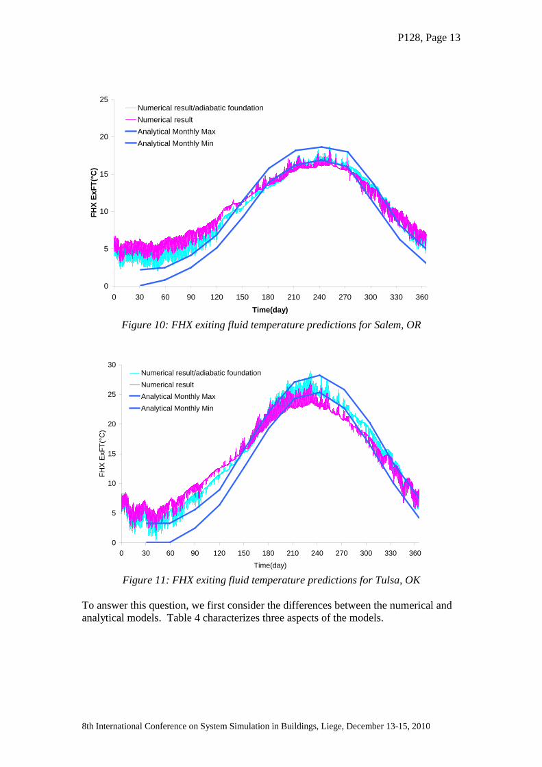
5. RESULTS Whether ground heat exchanger models are used for design or energy analysis, the key output is the exiting fluid temperature (ExFT), which is also the entering fluid temperature (EFT) for the heat pump. For design purposes, the minimum and maximum heat pump EFTs are the key design constraints that control the size of the ground heat exchanger. The analytical model, which is intended for use in design simulations, gives monthly minimum and maximum FHX ExFT, which are compared to ExFT generated by the numerical model in Figures 6-11 for the six locations. For all locations, the simulations are run with both models for a two year period and the second year simulation results are shown. By the second year, the results have essentially converged to a steady periodic result. Running the simulations for a third year will not change the minimum or maximum FHX ExFT more than 0.01°C compared with the second year. Figures 6-11 all show two sets of results for the numerical model and the maximum and minimum FHX ExFT for each month calculated with the analytical model. Ideally, the numerical results should vary between the minimum and maximum FHX ExFT for each month. The curves marked “Numerical result” represent the output from the numerical model as described above. The curves marked “Numerical result/adiabatic foundation” are from a modified version of the numerical model, described below, which will be used to help identify the sources of the differences between the numerical and analytical models.

P128,


0

5

10

15

20

25

30

0 30 60 90 120 150 180 210 240 270 300 330 360

Time(day)

FHX

ExFT

(°C

)Numerical result/adiabatic foundationNumerical resultAnalytical Monthly MaxAnalytical Monthly Min

Figure 6: FHX exiting fluid temperature predictions for Albuquerque, NM

For each case, the difference between the two models may be characterized in at least two ways. First, for a given length of FHX tubing, calculated with the analytical model, there will be a difference in the peak FHX ExFT calculated by the numerical model and the analytical model. This error in the analytical model prediction, treating the numerical model results as “correct” is summarized in Table 2. The "constraining HP EFT limit" is chosen to allow the system to operate within the limits specified by the manufacturer, within the limits of the working fluid, with acceptable capacity, and with acceptable energy efficiency. The temperature range for the heat pump operation chosen here is 0-40 °C as shown in Table 2. For each case, the peak FHX ExFT calculated by the analytical model exactly meets the constraining HP EFT limit.

Table 2: Peak FHX ExFT error

Locations Constraining HP EFT limit (°C)

Corresponding numerical model peak FHX ExFT

(°C)

Peak FHX ExFT error

(°C)

Salem 0.0 3.0 -3.0 Phoenix* 40.0 36.2 3.8

Albuquerque 0.0 1.5 -1.5 Knoxville 0.0 1.8 -1.8

San Francisco 0.0 2.4 -2.4 Tulsa 0.0 1.8 -1.8

* All cases except for Phoenix are constrained by the minimum HP EFT. Phoenix is constrained by the maximum HP EFT.

A second approach for characterizing the error is to compute the size (length) of FHX required to meet the heat pump entering fluid temperature constraints with both the

P128,


analytical model and the numerical model. In both cases, the models are applied iteratively and the length of the FHX is adjusted until either the minimum or maximum HP EFT limits are reached.

Table 3: FHX sizing error

Locations Constraining HP EFT limit

(°C)

FHX length sized with analytical model (m)

FHX length sized with numerical

model (m)

Error in analytical

model sizing

Salem 0.0 46.3 33.0 29% Phoenix 40.0 31.7 25.7 19%

Albuquerque 0.0 34.1 28.4 17% Knoxville 0.0 36.8 30.4 17%

San Francisco 0.0 18.0 14.5 19%

Tulsa 0.0 39.3 32.0 19% Looking at Tables 2 and 3, the errors are higher than desirable. While some oversizing by a simplified design tool is usually acceptable, errors as high as 29% are higher than desired. This leads to the question: why are the errors so high, particularly for the Salem, Oregon case?

0

5

10

15

20

25

30

0 30 60 90 120 150 180 210 240 270 300 330 360

Time(day)

FHX

ExFT

(°C

)

Numerical result/adiabatic foundation

Numerical result

Analytical Monthly Max

Analytical Monthly Min

Figure 7: FHX exiting fluid temperature predictions for Knoxville, TN

P128,


10

15

20

25

30

35

40

0 30 60 90 120 150 180 210 240 270 300 330 360

Time(day)

FHX

ExFT

(°C

)

Numerical result/adiabatic foundationNumerical resultAnalytical Monthly MaxAnalytical Monthly Min

Figure 8: FHX exiting fluid temperature predictions for Phoenix, AZ

0

5

10

15

20

25

30

0 30 60 90 120 150 180 210 240 270 300 330 360

Time(day)

FHX

ExFT

(°C

)


Figure 9: FHX exiting fluid temperature predictions for SanFrancisco, CA

P128,


0

5

10

15

20

25

0 30 60 90 120 150 180 210 240 270 300 330 360

Time(day)

FHX

ExFT

(°C

)


Figure 10: FHX exiting fluid temperature predictions for Salem, OR

0

5

10

15

20

25

30

0 30 60 90 120 150 180 210 240 270 300 330 360

Time(day)

FHX

ExF

T(°C

)


Figure 11: FHX exiting fluid temperature predictions for Tulsa, OK

To answer this question, we first consider the differences between the numerical and analytical models. Table 4 characterizes three aspects of the models.

P128,


Table 4: Comparison of numerical and analytical model features

Model Time step

Foundation wall geometry Ground temperature (UGT)

Numerical model hourly

Unconditioned basement with finite vertical and horizontal dimensions

Computed with numerical model and includes effects of

surface heat balance, soil freezing, and FHX heat

transfer

Analytical model monthly

Adiabatic foundation wall, infinite in the vertical direction

Determined with superposition – undisturbed

ground temperature portion is computed with Kusuda and

Achenbach model The effects of the three differences shown in Table 4 can be investigated by modifying the numerical model or the analytical model to be closer to each other. The first effect that we investigated is the foundation wall geometry. Because the analytical model cannot be modified to account for the actual geometry, we modified the numerical model to have an adiabatic foundation wall that was infinite in the vertical direction. These results are shown for every location in Figures 6-11 and are labeled “Numerical result/adiabatic foundation.” In all locations, except perhaps San Francisco, the numerical model with the adiabatic foundation comes much closer to the analytical model results. This indicates that the infinite adiabatic foundation wall assumption made by the analytical model is responsible for a significant amount of the error in the analytical model. Table 5 summarizes the peak FHX ExFT errors; compared to the results in Table 2, the peak FHX ExFT errors are nearly eliminated for Albuquerque, Knoxville and Tulsa. For San Francisco, Phoenix, and Salem, the errors are higher. Salem has the highest error and will be investigated further.

Table 5: Peak FHX ExFT error with adiabatic foundation

Locations Constraining HP EFT limit (°C)

Corresponding numerical model (with adiabatic

foundation) peak FHX ExFT (°C)

Peak FHX ExFT error

(°C)

Salem 0.0 2.0 -2.0 Phoenix 40.0 38.7 1.3

Albuquerque 0.0 0.2 -0.2 Knoxville 0.0 0.3 -0.3

San Francisco 0.0 1.8 -1.8 Tulsa 0.0 0.3 -0.3

As summarized in Table 4, the numerical model uses a heat balance on the surface to compute the ground temperature; the analytical model uses the Kusuda and Achenbach (1965) model to determine the undisturbed ground temperature. It is not feasible to implement a heat balance in the analytical model, but one possible approach is to compute the undisturbed ground temperature with a one-dimensional numerical model, then use it instead of the Kusuda and Achenbach-determined UGT within the analytical model. We have taken this approach, using a 1-d numerical model that has an identical surface heat balance to the FHX numerical model. The resulting UGT are used within the analytical model.

P128,


The results are shown in Figure 12; using the UGT computed with the 1-d numerical model eliminates most of the error. The peak error in FHX ExFT is reduced from -2°C (with the numerical model/adiabatic foundation) to -0.3°C. So, then most of the differences between the numerical model and the analytical model can be attributed to, first, the analytical model approximation of the basement as a vertical, infinite, adiabatic wall, and, second, use of the Kusuda and Achenbach model for undisturbed ground temperature. The Kusuda and Achenbach model does not account for freezing in the soil. Freezing in the soil limits the penetration of cold temperatures downwards and accounting for this may require a revised procedure. This is a subject of current investigation. It does seem that this is the most likely approach for improvement of the analytical model. Remaining differences are presumably due to differences in time steps: hourly loads for the numerical model and monthly loads and monthly peak loads for the analytical model. Further research may be needed to quantify the importance of these differences.

-5

0

5

10

15

20

25

0 30 60 90 120 150 180 210 240 270 300 330 360

Time(day)

FHX

ExFT

(°C

)

Numerical result/adiabatic foundationAnalytical Monthly Max/K&A UGTAnalytical Monthly Min/K&A UGTAnalytical Monthly Max/numerical UGTAnalytical Monthly Min/numerical UGT

Figure 12: Reasons for FHX ExFT difference between two model result in

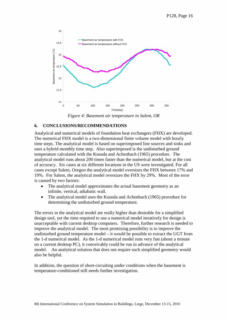
Salem,Oregon Also, for all of the cases shown above, the basement is not temperature conditioned. We expect that some “short-circuiting” will occur when the basement is conditioned and that remains a subject for future research. As a first attempt to look at the sensitivity of the basement to use of an FHX, consider Figure 13. Figure 13 shows the basement air temperature for a case without FHX (where the house heating and cooling are provided with another system) and the case with an FHX, in the second year of operation. The maximum difference is about 0.7°C; which seems acceptably small. However, how the short-circuiting will affect cases with conditioned basements is still under investigation.

P128,


11

11.5

12

12.5

13

13.5

14

0 50 100 150 200 250 300 350

Time(day)

Bas

emen

t air

tem

pera

ture

(°C

)

Basement air temperature with FHXBasement air temperature without FHX

Figure 4: Basement air temperature in Salem, OR

6. CONCLUSIONS/RECOMMENDATIONS Analytical and numerical models of foundation heat exchangers (FHX) are developed. The numerical FHX model is a two-dimensional finite volume model with hourly time steps. The analytical model is based on superimposed line sources and sinks and uses a hybrid monthly time step. Also superimposed is the undisturbed ground temperature calculated with the Kusuda and Achenbach (1965) procedure. The analytical model runs about 200 times faster than the numerical model, but at the cost of accuracy. Six cases at six different locations in the US were investigated. For all cases except Salem, Oregon the analytical model oversizes the FHX between 17% and 19%. For Salem, the analytical model oversizes the FHX by 29%. Most of the error is caused by two factors:

• The analytical model approximates the actual basement geometry as an infinite, vertical, adiabatic wall.

• The analytical model uses the Kusuda and Achenbach (1965) procedure for determining the undisturbed ground temperature.

The errors in the analytical model are really higher than desirable for a simplified design tool, yet the time required to use a numerical model iteratively for design is unacceptable with current desktop computers. Therefore, further research is needed to improve the analytical model. The most promising possibility is to improve the undisturbed ground temperature model – it would be possible to extract the UGT from the 1-d numerical model. As the 1-d numerical model runs very fast (about a minute on a current desktop PC), it conceivably could be run in advance of the analytical model. An analytical solution that does not require such simplified geometry would also be helpful. In addition, the question of short-circuiting under conditions when the basement is temperature-conditioned still needs further investigation.

P128,


ACKNOWLEDGEMENT

Financial support of the U.S. Department of Energy is gratefully acknowledged.

REFERENCES Antonopoulos, V. Z. 2006. Water movement and heat transfer simulations in a soil

under ryegrass. Journal of Biosystems Engineering 95(1): 127-138. Bose, J. E., J. D. Parker, and F. C. McQuiston. 1985. Design/data Manual for closed-

loop ground coupled heat pump systems, Atlanta:ASHRAE. Braven, D., and E. Nielson. 1998. Performance prediction of a sub-slab heat

exchanger for geothermal heat pumps. Journal of Solar Energy Engineering, Transactions of the ASME 120: 282-288.

Briggs, R. S., R.G. Lucas, and T. Taylor. 2003. Climate Classification for Building Energy Codes and Standards: Part 1 - Development Process. ASHRAE Transactions 109: 109-117.

Chang, J. H. 1958. Ground Temperature. Bluehill Meteorological Observatory, Harvard University

Collins, W. D. 1925. Temperature of water available for industrial use in the United States. United States Geological Survey Water Supply Paper 520-F, Washington: USGS

Cullin, J. 2008. Improvements in design procedures for ground source and hybrid ground source heat pump systems. M.S. Thesis. Oklahoma State University.

Gao, J., X. Zhang, J. Liu, K. Li, and J. Yang. 2008. Numerical and experimental assessment of thermal performance of vertical energy piles: An application. Applied Energy 85(10): 901-910.

Kusuda, T., and P. R. Achenbach. 1965. Earth Temperature and Thermal Diffusivity at Selected Stations in the United States. ASHRAE Transactions 71(1): 61-76.

Lamberg, P., R. Lehtiniemi, and A. M. Henell. 2004. Numerical and experimental investigation of melting and freezing processes in phase change material storage. Internation Journal of Thermal Sciences 43(3).

Mei, V. C. 1985. Theoretical heat pump ground coil analysis with variable ground farfield boundary conditions. AlChE Symposium Series(245): 7-12.

Mei, V. C. 1988. Heat pump ground coil analysis with thermal interference. Journal of Solar Energy Engineering, Transactions of the ASME 110(2): 67-73.

Mei, V. C., and C. J. Emerson. 1985. New approach for analysis of ground-coil design for applied heat pump systems. ASHRAE Journal 91(2): 1216-1224.

Niu, G. Y., and Z. L. Yang. 2006. Effects of frozen soil on snowmelt runoff and soil water storage at a continental scale. J. Hydrometeorol. 7(5): 937-952.

Piechowski, M. 1998. Heat and mass transfer model of a ground heat exchanger: Validation and sensitivity analysis. International Journal of Energy Research 22(11): 965-979.

Piechowski, M. 1999. Heat and mass transfer model of a ground heat exchanger: Theoretical development. International Journal of Energy Research 23(7): 571-588.

Spitler, J. D. 2000. A design tool for commercial building ground loop heat exchangers. Proceedings of the Fourth International Heat Pumps in Cold Climates Conference, Aylmer, Québec

P128,


Walter, I. A., R. G. Allen, R. Elliott, D. Itenfisu, P.Brown, M. E. Jensen, B. Mecham, T. A. Howell, R. Snyder, S.Eching, T.Spofford, M.Hattendorf, D.Martin, R.H.Cuenca, and J. L. Wright. 2005. The ASCE standardized reference evapotranspiration equation. Standardization of Reference Evapotranspiration Task Committee Final Report. American Society Civil Engineers. Environmental and Water Resources Institute.

Xing, L. 2010. Analytical and numerical modeling of foundation heat exchangers. M.S. Thesis. Oklahoma State University. Stillwater.

modeling of foundation heat exchangers · modeling of foundation heat exchangers is similar to...

Documents