modeling of generation and distribution of steam in an autoclave

i

Modeling of Generation and Distribution of Steam in an Autoclave A CFD Analysis

Master of Science Thesis

PER HAMLIN

Department of Chemical and Biological Engineering Division of Chemical Engineering CHALMERS UNIVERSITY OF TECHNOLOGY Göteborg, Sweden, 2012

ii


PER HAMLIN

Department of Chemical and Biological Engineering Division of Chemical Engineering

CHALMERS UNIVERSITY OF TECHNOLOGY Göteborg, Sweden, 2012

iii


PER HAMLIN

© PER HAMLIN, 2012.

Department of Chemical and Biological Engineering Chalmers University of Technology SE-412 96 Göteborg Sweden Telephone + 46 (0)31-772 1000

Cover: a. Path lines of the evaporating flow in the modeled steam generator. b. Contours of air mole fraction in the modeled sterilization chamber.

Göteborg, Sweden 2012

iv


PER HAMLIN

Department of Chemical and Biological Engineering Chalmers University of Technology

ABSTRACT

Sterilization of tools and equipment in order to prevent the spread of germs, bacteria and viruses is of great importance in the medical field. This can be accomplished by using an autoclave, a device that sterilizes tools and equipment with the help of steam. The generation of steam in the steam generator and distribution of steam in the sterilization chamber has been treated theoretically and numerically in this thesis. Numerical analysis has also been executed with the help of CFD.

An extensive literature review has been conducted regarding the droplet boiling mechanisms, nucleate boiling and droplet-wall interaction in the steam generator. In addition, relevant theory of transport phenomena and CFD are presented. Key parameters were identified and estimated in detail. With the help of theoretical framework and key parameters, suitable computational models were selected and analyzed.

With respect to nucleate boiling, there were no suitable models that could be applied to the problem on hand. Steam generation was therefore modeled using assumed fluid properties to increase heat transfer and the rate of evaporation. In general, realistic results were obtained but complete validation was not possible due to lack of detailed experimental data. In addition, a droplet boiling model framework has been presented for future modeling of nucleate boiling with the discrete particle method.

The general trends of steam distribution inside the sterilization chamber were analyzed in multi component single phase simulations. The feasibility of modeling high rates of condensation was successfully shown with regards to simplified simulations.

Keywords:

CFD, Multiphase Flow, Steam Generator, Sterilization

v

PREFACE This Master’s Thesis has been made in cooperation with Getinge Skärhamn AB, Technical Analysis at ÅF, Göteborg and the Division of Chemical Engineering at Chalmers University of Technology, Göteborg.

Acknowledgments I would like to thank

Vijay Shankar, my supervisor at ÅF

Ronnie Andersson, my examiner at Chalmers University of Technology

Gert Linder, Getinge Skärhamn AB

Johan Wanselin, Getinge Skärhamn AB

Andreas Lindqvist, Getinge Skärhamn AB

Magnus Christiansson, Getinge Skärhamn AB

Sven Hillberg, Getinge Skärhamn AB

Göteborg, November 18, 2012

Per Hamlin

vi

NOMENCLATURE

A Area C Constant c Molar concentration

CP Specific heat capacity

D Diameter DAB Mass diffusivity

F Force F Frequency

gi Gravity term

h Heat transfer coefficient

h Enthalpy

k Thermal conductivity

k Turbulent kinetic energy

kc Mass transfer coefficient

Kn Knudsen number L Length M Molar mass

m Mass Mass flow rate

N Molar flux

n Mole Nu Nusselt number NW Nucleate site density

P Pressure Pr Prandtl number q Heat transfer Re Reynolds number S Source term Sh Sherwood number St Stokes number T Temperature t Time u Velocity

V Volume Volumetric flow rate

We Weber number x x-component length y Mole fraction y y-component length y+ Wall

Greek Symbols ∆Hvap Heat of vaporization

ɛ Dissipation rate

δ Film thickness δij Delta function λ Mean free path μ Viscosity ρ Density

σ Stefan-Boltzmann constant

σST Surface tension

τ Time φapp Apparent contact angle ω Specific dissipation rate

Subscripts A Species A air Air alu Aluminum b Bubble B Species B

vii

bc Boundary condition Bouy Buoyancy Bp Boiling point Brown Brownian cell Cell ch Channel cond Conduction conden Condensation conv Convection d Droplet Drag Drag eff Effective evap Evaporation F Flow given Given Heat Heat History History i Directional tensor notation in Inlet j Directional tensor notation k Directional tensor notation l Largest scales of turbulence Lift Lift liq Liquid load Tray loading material meas Measured mom Momentum out Outlet Press Pressure que Quenching rad Radiation SC Sterilization chamber SG Steam generator St Steam steel Steel surf Surface T Turbulent Therm Thermophoretic tot Total tray Tray v Vapor Virt Virtual w Water wall Wall x x-direction η Smallest scales of turbulence (Kolmogorov)

viii

TABLE OF CONTENTS ABSTRACT ............................................................................................................................................................... iv

PREFACE ................................................................................................................................................................... v

Acknowledgments ............................................................................................................................................... v

NOMENCLATURE .................................................................................................................................................... vi

Greek Symbols .................................................................................................................................................... vi

Subscripts ............................................................................................................................................................ vi

1. INTRODUCTION .............................................................................................................................................. 1

1.1 Background ................................................................................................................................................... 1

1.2 Objective ....................................................................................................................................................... 1

1.3 Demarcations ................................................................................................................................................ 1

1.4 Investigation of Key Parameters ................................................................................................................... 1

2. AUTOCLAVES .................................................................................................................................................. 2

2.1 Process Description....................................................................................................................................... 3

2.2 Steam Generator .......................................................................................................................................... 4

2.3 Sterilization Chamber ................................................................................................................................... 5

2.4 Vacuum System ............................................................................................................................................ 6

3. THEORETICAL FRAMEWORK .......................................................................................................................... 7

3.1 Transport Phenomena .................................................................................................................................. 7

3.1.1 Dimensionless Numbers ........................................................................................................................ 7

3.1.2 Heat Transfer ......................................................................................................................................... 7

3.1.3 Mass Transfer ........................................................................................................................................ 8

3.1.4 Fluid Mechanics ..................................................................................................................................... 8

3.1.5 Phase Change ........................................................................................................................................ 8

3.1.6 Droplet-Wall Interaction ..................................................................................................................... 13

3.2 Computational Fluid Dynamics Modeling ................................................................................................... 15

3.2.1 Geometry and Meshing ....................................................................................................................... 15

3.2.2 Governing Equations ........................................................................................................................... 15

3.2.3 Numerical Aspects ............................................................................................................................... 16

3.2.4 Turbulence Modeling .......................................................................................................................... 17

3.2.5 Multiphase Modeling .......................................................................................................................... 19

3.2.6 Boundary Conditions ........................................................................................................................... 22

4. METHOD ....................................................................................................................................................... 24

4.1 Hand Calculations ....................................................................................................................................... 24

4.2 Geometry .................................................................................................................................................... 24

4.2.1 Steam Generator ................................................................................................................................. 24

4.2.2 Sterilization Chamber .......................................................................................................................... 25

ix

4.3 Meshing ...................................................................................................................................................... 26

4.3.1 Steam Generator ................................................................................................................................. 26


4.4 Simulation Setup ......................................................................................................................................... 28

4.4.1 Steam Generator ................................................................................................................................. 28


5. RESULTS ........................................................................................................................................................ 32

5.1 Steam Generator ........................................................................................................................................ 32

5.1.1 Single Phase Simulations: Choice of Turbulence Model ...................................................................... 32

5.1.2 Discrete Particle Method: Selection of Boundary Conditions ............................................................. 36

5.1.3 Discrete Particle Method: Full Steam Channel .................................................................................... 42

5.2 Sterilization Chamber ................................................................................................................................. 46

5.2.1 Single Phase Simulations ..................................................................................................................... 46

5.2.2 Multiphase Simulations ....................................................................................................................... 48

6. RECOMMENDATIONS FOR DEVELOPMENT OF A DROPLET BOILING MODEL ............................................ 49

6.1 Droplet-Wall Impact and Interaction .......................................................................................................... 49

6.2 Boiling Regimes ........................................................................................................................................... 49

6.2.1 Evaporation Regime ............................................................................................................................ 49

6.2.2 Nucleate Boiling Regime ...................................................................................................................... 49

6.2.3 Film and Transition Boiling Regime ..................................................................................................... 50

7. DISCUSSION ................................................................................................................................................. 51

7.1 Steam Generator ........................................................................................................................................ 51


8. CONCLUSION ................................................................................................................................................ 54

8.1 Steam Generator ........................................................................................................................................ 54


8.3 General Summary ....................................................................................................................................... 54

8.4 Future Work ................................................................................................................................................ 54

9. REFERENCES ................................................................................................................................................. 56

APPENDIX 1: Sterilization Process Measurements .............................................................................................. 59

APPENDIX 2: User Defined Functions .................................................................................................................. 61

APPENDIX 3: Sterilization Chamber Single Phase Results ................................................................................... 62

APPENDIX 4: Basic Concepts of Fluid Mechanics................................................................................................. 63

APPENDIX 5: Hand Calculations ........................................................................................................................... 65

APPENDIX 6: Tabular Results ............................................................................................................................... 73

1

1. INTRODUCTION In this section, backgrounds to the problem on hand, as well as the key objectives are described. The demarcations and research questions of the same are also presented.

1.1 Background Sterilization of tools and equipment to prevent the spread of germs, bacteria and viruses is of great importance in the medical field. This can be accomplished by using an autoclave, a device that sterilizes tools and equipment with the help of steam.

Getinge Skärhamn is a world leading manufacturer of small and medium sized autoclaves for medical and laboratory use. In order to maintain its leading position on the market, the company is aiming for continuous research and development to further improve their products. The company’s aim is to provide autoclaves with shorter sterilization cycles or so called high speed sterilization processes. It is also highly desired to minimize the volume and weight of the autoclave.

The process consists of steam injection into the sterilization chamber and vacuum suction of the same. The steam generator consists of a heated aluminum block in which steam is generated instantly as pressurized water is sprayed onto the heated aluminum wall. The vacuum system has a steam condenser and a membrane pump as its main components.

With the help of Computational Fluid Dynamics (CFD), it is possible to investigate important system characteristics in order to improve the time of sterilization and minimize the volume and weight of the autoclave.

1.2 Objective The following are the main objectives of this thesis work.

a. Theoretical description of nucleate boiling with respect to steam generation. b. Numerical analysis of steam generation in an autoclave. c. CFD analysis of steam distribution in the sterilization chamber in an autoclave.

1.3 Demarcations The thesis work is based on numerical analysis of Getinge Skärhamn’s table-top autoclave in the Quadro product series. The steam generator and the distribution of steam in the sterilization chamber will be modeled. Necessary simplifications and assumptions and will be implemented during modeling with the help of CFD.

1.4 Investigation of Key Parameters The following are the main topics questions that need to be analyzed during the course of this thesis work.

a. How is the steam produced in the existing steam generator? b. How can the steam generation be modeled with the help of CFD? c. How is steam distributed in the sterilization chamber? d. How can the distribution of steam be analyzed with the help of CFD?

2

2. AUTOCLAVES Autoclaves are used to sterilize tools and equipment in medical, dental and laboratory environments by treatment with high temperature steam. Prior to the use of autoclaves, sterilization was frequently performed using boiling water at , an insufficient treatment as many bacteria and microorganisms survive temperatures up to . The steam temperature of the autoclave must therefore exceed to reach adequate sterilization (Vårdhandboken, 2011). According to present regulations, a temperature of must be upheld for at least 3 minutes inside the sterilization chamber. The pressure inside the sterilization chamber is increased in order to obtain dry saturated steam with the temperature suitable for sterilization. Autoclaves of various sizes exist ranging from tabletop to room-sized autoclaves. The autoclave investigated in this thesis is of tabletop size and is shown in Fig. 1.

Fig. 1. Getinge Skärhamn's tabletop Quadro autoclave. Five trays can be loaded into the 18 liter sterilization chamber.

Getinge Skärhamn’s tabletop Quadro-series autoclaves are available with a chamber volume of liters. The main components of the autoclave, namely the steam generator, sterilization chamber and vacuum system, can be seen in the steam generation flow scheme, shown in Fig. 2. The named components and the sterilization process are described below but for full product specifications see Getinge Skärhamn’s website. The goods to be sterilized are put on trays which are wrapped in a protecting pouch prior to being loaded into the sterilization chamber. A maximum of five trays loaded with goods can be sterilized during one cycle, as shown in Fig. 3. While maintaining adequate sterilization, Getinge Skärhamn aims at decreasing the size and weight of the autoclave as well as cutting the process cycle time to remain competitive on the market.

3

Fig. 2. Flow scheme of steam generation (Capitao et al., 2010). The main components are shown: steam generator (Ångalstrare), sterilization chamber (Sterilisationskammare) and vacuum system (Kondensor med fläkt and Ejektor). The labels in the figure are in Swedish

1.

Fig. 3. A loaded sterilization chamber of Getinge Skärhamn's Quadro autoclave.

2.1 Process Description The normal sterilization process applied by Getinge Skärhamn’s Quadro-series takes approximately 30 minutes and can be divided into three stages: the pre-process phase, the sterilization phase, and the drying phase. Pressure and temperature operating conditions of one sterilization cycle can be seen in Fig. 4.

1 “Processkarta over ångalstringsprocessen” = Process scheme of the steam generation process. “Vattentank” =

Water tank. “Magnetventil” = Magnetic valve. ”Pump” = pump. ”Ångalstrare” = steam generator. ”Sterilisationskammare” = sterilization chamber. ”Kondensor med fläkt" = Condenser with fan. ”Bakventil” = Check valve. ”Ejektor” = ejector.

4

Fig. 4. Process data from a standard sterilization process in the Quadro autoclave. The labeled pressures and temperatures are displayed as a function of process time in minutes.

At first when the pre-process phase is initiated, the sterilization chamber is completely filled with air. To allow steam to penetrate the entire chamber volume including inside the trays, air must be removed. The vacuum system sucks air from the chamber and a low pressure environment of approximately is obtained. Steam is then generated in the steam generator and enters the chamber, which in turn increases the pressure to approximately again. This procedure, referred to as vacuum pulsation, is repeated several times to ensure maximum removal of air. The pre-process phase takes approximately 15 minutes which is around half of the total process cycle.

Secondly, the sterilization phase is initiated through the generation and addition of steam until a working temperature of is reached. To allow extensive steam treatment and sterilization, this working temperature is maintained for several minutes. The sterilization phase takes at least 3 minutes but since regulations govern the time extent of this phase, the same cannot be shortened.

Thirdly, the drying phase is then initiated. An exit valve in the sterilization chamber is opened whereby steam reaches the condenser and condenses. This creates a pressure gradient that sucks steam out of the chamber until the pressure is well below , the vacuum pump then compliments the condenser and lowers the pressure further. Low pressure is maintained for some time to allow sufficient drying. Finally, air is entered into the chamber until atmospheric pressure is reached and the sterilization process is completed. The drying phase takes approximately 10 minutes which is approximately one third of the total process cycle.

2.2 Steam Generator The autoclave is powered through a standard wall electricity socket which means that the instantaneous maximum power supply is limited. At full steam production the power demand is several times larger than the available supply, thus energy must be buffered in order for enough steam to be generated at peak loads

2. The

steam generator (see Fig. 5) consists of an electrically heated aluminum block weighing approximately , enabling storage of a sufficient amount of energy. The electrical heaters are regulated against a set value of , but during peak loads the temperature will drop to nearly in parts of the aluminum block

3. The

block is penetrated by a channel into which water is sprayed with an injector nozzle. The water is evaporated through heat transfer from the hot surfaces of the aluminum block. The steam then exits the steam generator and enters the sterilization chamber.

2 Personal communication with Johan Wanselin, development manager at Getinge Skärhamn.

3 Personal communication with Andreas Lindqvist, designer at Getinge Skärhamn.

5

Fig. 5. CAD model of the steam generator or heat accumulator. The left hand figure depicts the aluminum block with the steam channel in the center. The right hand figure includes the two electrical heaters as well as the fittings to the steam channel.

The walls of the steam channel are treated with a calcium hydroxide aqueous solution prior to assembling the autoclave. The treatment lasts for several hours until a sufficiently thick, porous and rough deposit coats the surface

4. The reason for adding this surface finish is for droplets to enter the nucleate boiling regime, to avoid

the Leidenfrost phenomena and maintain high heat transfer rates (further described in Phase Change below). With no surface treatment most of the injected liquid droplets will not evaporate and there will be an insufficient steam flow rate into the chamber

5.

2.3 Sterilization Chamber The sterilization chamber (see Fig. 6) is a pressure vessel designed to withstand pressures up to 5

6. The

geometry of the chamber is a trade-off between the durability of a cylindrical shape and the loading capacity of a rectangular shape. The chamber door is sealed with rubber gaskets to prevent leakage. A circular metal disk is fastened in the back of the chamber as shown in Fig. 7. The steam from the inlet thus hits the disk prior to escaping into the chamber through the narrow gaps between the circular disk and slightly asymmetrical chamber. The goods to be sterilized is put on trays and inserted into the chamber prior to the sterilization cycle as seen in Fig. 3 above.

Fig. 6. CAD model of the sterilization chamber. The left hand figure depicts the chamber including fittings as well as the chamber door. The right hand figure depicts only the chamber itself.

4 Personal communication with Andreas Lindqvist, designer at Getinge Skärhamn.



6

Fig. 7. The sterilization chamber including the circular metal disk preventing steam from entering the chamber directly from the steam generator.

2.4 Vacuum System The vacuum system creates a low pressure zone (vacuum) in the sterilization chamber. Although this pressure ( ) is strictly defined as low vacuum it is in this report referred to as vacuum. Vacuum is generated in two ways: by a membrane vacuum pump and by condensation of steam. When the chamber is filled with air, the membrane pump generates an under-pressure sucking air out of the system. In contrary, when the chamber is filled with steam, steam condenses in the condenser generating an under-pressure that sucks steam out of the system.

7

3. THEORETICAL FRAMEWORK In this section relevant transport phenomena as well as CFD theory are presented. The theoretical framework is based on relevant literature study.

3.1 Transport Phenomena The modeled systems contain several modes of heat, mass and momentum transfer. For basic understanding of these mechanisms on both the microscopic and macroscopic scales, relevant transport phenomena will be presented in this section.

3.1.1 Dimensionless Numbers The idea of dimensionless numbers is to group problem specific variables into dimensionless parameters and thus reduce the number of independent variables (Welty et al., 2008). The dimensionless parameters can be used to relate different properties such as forces, diffusivity, time constants etc. and in correlations. The dimensionless numbers of importance to this thesis are listed in Table 1 below.

Table 1. The dimensionless numbers that are of importance to this thesis.

Dimensionless Number Definition

Reynolds number

Nusselt number

Sherwood number

Prandtl number

Schmidt number

Stokes number

Weber number

Knudsen number

3.1.2 Heat Transfer Heat transport is essentially the transport of energy, of which there are three types: conductive, convective and radiant heat transfer. These are listed in Table 2 below.

Table 2. The three types of heat transfer mechanisms.

Heat Transfer Mechanism Definition

Conduction

Convection

Radiation

8

3.1.3 Mass Transfer When species concentrations vary in a system there is a natural driving force for mass to be transferred until concentration differences are minimized. There are two ways in which mass can be transported: diffusive mass transfer and convective mass transfer. These are defined as in Table 3.

Table 3. The two types of mass transfer mechanisms.

Mass Transfer Mechanism Definition

Diffusion

Convection

3.1.4 Fluid Mechanics Studying momentum transport in a fluid implies the study of motion of the fluid and the forces producing these motions, historically also referred to as fluid mechanics (Welty et al., 2008). Some important concepts of fluid mechanics including laminar and turbulent flow, compressible and incompressible flow and boundary layers are important to this thesis. Basic theoretical descriptions of these concepts are presented in Appendix 4.

3.1.5 Phase Change Steam is widely used in various applications due to its properties. It is an excellent non-corrosive energy carrier that is perfectly suitable for use in sterilization applications. When the boiling temperature of water is reached at constant pressure, the temperature is constant until all of the water has been evaporated. In this situation there is equilibrium between the liquid and gas phases, thus they have the same temperature and pressure referred to as the saturation temperature and saturation pressure respectively (Elliot and Lira, 2006). The heat required to vaporize a liquid into its gas phase is called the latent heat or heat of vaporization ( ). Water’s

heat of vaporization is

(Mörstedt and Hellsten, 2008). If further heat is supplied when all water has

been evaporated, the steam is superheated and behaves like conventional gases at high temperatures. The saturation temperature of water is a function of pressure; the general relation is given by the saturation curve in Fig. 8.

Fig. 8. The steam saturation temperature curve as a function of pressure.

9

Likewise, when saturated steam comes in contact with a cold surface it starts condensing on and heating the surface. The amount of energy released is equivalent to the heat of vaporization. Condensation will continue until the surface has been heated to the steam’s saturation temperature or until all steam has condensed. Both film condensation where the liquid spreads and wets the surface and drop wise condensation where the liquid forms droplets and runs across the surface can occur (Welty et al., 2008).

Dispersed Droplet Evaporation Dispersed droplets are subject to mass, heat and momentum exchange with the gaseous phase. Many studies have been performed on internal droplet transport phenomena but these effects are mostly neglected in this thesis, the interested reader is referred to Ashgriz (2011). In the numerical simulations, the droplet, is assumed to be spherical and with a homogeneous internal temperature profile. Heat transfer to and from the droplet can be described by the classical transport mechanisms presented in Heat Transfer earlier. When considering a single species droplet there will only be interfacial mass transfer at the surface as liquid evaporates. The droplet diameter can then be determined by the so called d-squared law where the square of the droplet diameter as a function of time (Ashgriz, 2011). One must also consider the heat of vaporization in heat transfer since this produces a heat sink in the remaining liquid and surrounding gas. Dispersed droplet evaporation is quite slow compared to wall boiling whereas it is not of great significance in this thesis. This is determined by hand calculations in Appendix 5, through the calculation of the different particle Stokes numbers, particle response times etc.

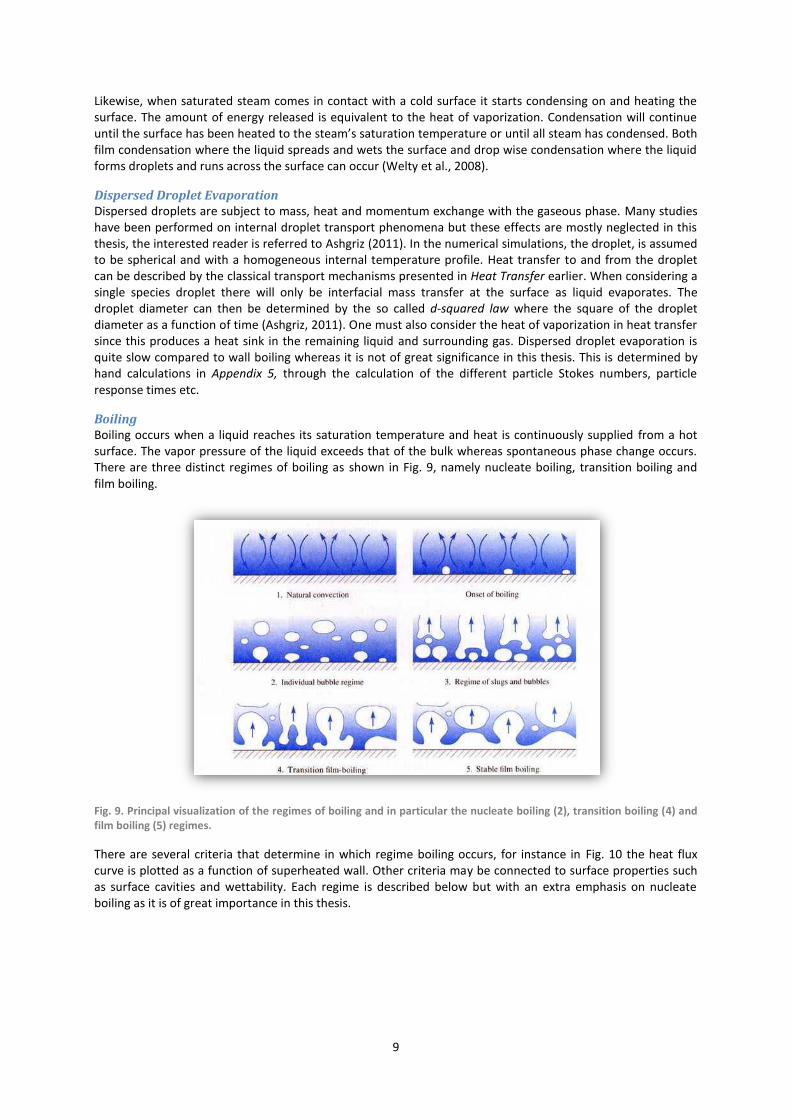
Boiling Boiling occurs when a liquid reaches its saturation temperature and heat is continuously supplied from a hot surface. The vapor pressure of the liquid exceeds that of the bulk whereas spontaneous phase change occurs. There are three distinct regimes of boiling as shown in Fig. 9, namely nucleate boiling, transition boiling and film boiling.

Fig. 9. Principal visualization of the regimes of boiling and in particular the nucleate boiling (2), transition boiling (4) and film boiling (5) regimes.

There are several criteria that determine in which regime boiling occurs, for instance in Fig. 10 the heat flux curve is plotted as a function of superheated wall. Other criteria may be connected to surface properties such as surface cavities and wettability. Each regime is described below but with an extra emphasis on nucleate boiling as it is of great importance in this thesis.

10

Fig. 10. The boiling regime heat flux curve (Mudawar and Valentine, 1989). The curve includes the evaporation, nucleate boiling, transition boiling and film boiling regimes as a function of wall superheat. The ONB, CHF and LP are clearly labeled in the graph.

Nucleate Boiling The nucleate boiling regime is characterized by the formation, growth and departure of vapor bubbles at a heated wall or surface. Vapor bubble nuclei form at nucleation sites on the surface and grow as heat supply induces evaporation. When the bubble diameter is large enough it breaks off and rises from the wall through the boundary layer (Zeng et al., 1993) until either condensing or reaching the bulk. Subsequently a new bubble nuclei forms at the surface site and the procedure is repeated. As evident in Fig. 10 nucleate boiling is characterized by the exponential heat flux increase with an increase in wall superheat. This makes nucleate boiling extremely interesting for high performance heat transfer and cooling applications (Mudawar and Valentine, 1989; Narumanchi et al., 2007). The regime is however bounded by the Onset of Nucleate Boiling (ONB) and Critical Heat Flux (CHF) points. The nucleate boiling regime can be observed in various flow situations such as pool boiling, flow boiling and impinging droplet boiling (Bernardin et al., 1997). Although much research has been performed in the nucleate boiling field all the involved mechanisms are not completely understood or known of, reported mechanisms of nucleate boiling are described below.

Heat and Mass Transfer Phenomena To understand the process of nucleate boiling one must examine both the microscopic and macroscopic heat and mass transfer mechanisms (Stephan and Kern, 2004; Stephan and Fuchs, 2007). The space in between vapor bubbles or nucleation sites is simply comprised of a purely liquid film in contact with the surface whereas single phase transport phenomena are expected to govern heat and mass transfer (see Heat Transfer and Mass Transfer above). It has also been concluded that the transport phenomena within the bubbles are rather insignificant to the total heat flux (Krupiczka et al., 2000) and therefore the transport phenomena related to the vapor bubble interface and its immediate surroundings is of interest. Fig. 11 shows a single bubble at a surface nucleation site surrounded by liquid. As labeled in the figure the phase interface can be divided into the adsorbed liquid film, micro and macro regions (Stephan and Kern, 2004). This concept enables the study of several microscopic transport phenomena described below.

11

This main transport mechanism during bubble growth is described in this paragraph. Thermal conductivity of water is small compared to most metals and the thermal resistance will thus be quite large in the macro region. However as the film thickness ( ) decreases the thermal resistance also decreases whereas more heat will flow through the micro region compared to the macro one. The thin liquid film will, due to the high heat flux be superheated and in addition the adhesion pressure and phase interface curvature resulting from the decreasing film thickness will decrease volatility (Stephan and Kern, 2004). The rate of evaporation will thus be high in the micro region. The adsorbed liquid film under the bubble will however not evaporate due to strong adhesion forces (Stephan and Fuchs, 2007). Of the total heat transfer, evaporative heat transfer is the most dominant in nucleate boiling (Stephan and Kern, 2004). As liquid evaporates from the microscopic film its thickness should assumedly decrease. However, adhesion forces implicate continuous wetting of the surface which induces a flow from the macro into the micro region (labeled transverse flow in Fig. 11). Evaporation adds vapor to the bubble increasing its’ buoyancy until it reaches a critical size whereby it detaches from the nucleation site and departs through the boundary layer.

Fig. 11. Schematic figure of a single bubble and important transport phenomena during nucleate boiling (Stephan and Kern, 2004). The bottom figure is a magnification of the bubble-wall intersection.

There is also several transport mechanisms related to bubble departure including the ones presented in this paragraph. The bubble departure diameter has been studied by Zeng et al. (1993) through the setting up of a force balance over the bubble with the bubble growth rate as only closure. Genske and Stephan (2006) however reported that the departure diameter is dependant of the apparent contact angle, labeled in Fig.

11, with larger departure diameters resulting from larger contact angles. This provides vital input into nucleate boiling computational models such as the RPI Boiling Model presented later. As the bubble leaves the nucleation site liquid fills the void resulting from its departure. This increases liquid mixing near the wall whereby it enhances convective heat transfer and has been called quenching heat flux. Quenching heat flux is, as concluded later below, a significant part of the total wall heat flux in nucleate boiling. There is yet another microscopic heat transfer mechanisms within the boundary layer that results from the bubble departure called micro-convection. This is the result of superheated liquid from the adsorbed film being entrained in the departing bubble wake. This addition to total heat transfer will however be negligible on a global scale. On the macroscopic scale latent heat is carried from the boundary layer as the bubble departs into the bulk. In a sub-cooled boiling situation the bubble would condense and thereby adding its latent heat to the bulk while in liquid film boiling the bubble would escape to the gaseous bulk and thus adding the latent heat to its inner energy. In addition, Stephan and Kern (2004) reported that bubbles sliding across walls in in-cylinder boiling due to gravity force may have significant impact on total heat transfer.

12

Surface tension or interfacial tension forces act to maintain the bubble interface between the liquid and vapor. When liquid evaporates at the interface the interfacial tension is temporarily altered creating surface tension gradients which in turn induce a transverse flow over the surfaces. This phenomenon is called the thermo-capillary or Marangoni effect. The induced flow affects convective heat transfer into the surrounding liquid. This effect has been known of but in most literature on nucleate boiling assumed not to affect boiling heat transfer (Stephan and Kern, 2004). Recently, this assumption has been questioned as the Marangoni heat transfer has been shown to be comparable to buoyancy driven convection at certain levels of heat flux during nucleate boiling (Petrovic et al., 2004).

In short, both microscopic and macroscopic transport phenomena are significant for the total heat and mass transfer in nucleate boiling. Computational models of nucleate boiling are often based on a coupling of microscopic and macroscopic transport phenomena. Apart from the single phase transport in the macro region, these models are based on the thin liquid film evaporation model as described above (Krause et al., 2010). There is a general agreement in literature that heat transfer from the wall can be sufficiently approximated by three constituents (Tong, 1971; Krepper et al., 2006; Podowski, 2008) namely:

a. Convective heat transfer from wetted surface in between vapor bubbles. b. Enhanced convection when liquid fills void of detaching vapor bubble. c. Evaporative heat transfer.

These three mechanisms of heat transfer have for example been implemented into FLUENT in the RPI Boiling Model (below). Heat transfer correlations for different flow situations have been proposed by among others Tong (1971), Mudawar and Valentine (1989), Das et al. (2007) and Podowski (2008).

Surface Properties Since sequential bubble nucleation is the main characteristic of nucleate boiling, knowledge about how surface properties affect bubble nucleation, growth and detachment is therefore essential. Numerous articles have reported that nucleate boiling is greatly affected by the characteristics of the surface at which boiling occurs (Baumeister et al., 1970; Narumanchi et al., 2007; Yagov, 2009). Firstly fundamental aspects such as material thermal conductivity and heat capacity are important to consider. Secondly and more importantly for nucleate boiling theory is the surface structure including surface topography, shape of cavities, nucleation site density, surface wettability, fouling and coating (Dhir and Liaw, 1989). There is general agreement in literature that all nucleate boiling computational models need tuning to experimental data before predictive results can be obtained (Mei et al., 1995; Das et al., 2006).

Surface topography or roughness has been reported to affect nucleate boiling. Although more importantly than surface topography for flow boiling is the presence and frequency of micro cavities or nucleation sites as is described in the next paragraph. However an increase in surface roughness most often implies an increase in surface cavity density. Surface topography and roughness is however an essential property to consider in the case of impacting droplet boiling (Bernardin et al., 1997), this discussion is extended in Droplet-Wall Interaction below.

Nucleation sites are typically small surface cavities providing space in which bubbles can grow. Cavity density and sizes are, unless the surface has been carefully finished, heterogeneous and difficult to even theoretically describe on a macroscopic level (Yagov, 2009). The shape and size of the cavity will affect the departing bubble diameter which has great effects on the total heat flux from the wall. With two or more nucleation sites being close enough bubbles may interact or coalescence to form slugs of vapor (Podowski, 2008). This adds extra complexity in describing the already difficult nucleation process. Mosdirf and Shoji (2004) reported that interaction between adjacent nucleation sites can increase bubble departure frequency. It has in fact been reported that the assumption of bubbles being isolated during nucleate boiling is poor (Luke, 2010). A comparison of boiling on plain and on structured surfaces with artificial micro-drilled cavities revealed that heat flux increases with nucleation site density and that fine tuning correlations to case specific surfaces is needed (Das et al., 2006). That heat flux increases with nucleation site density is fairly intuitive and has also been reported by Genske and Stephan (2006).

Surface wettability has been reported to greatly affect the nucleate boiling heat transfer (Dhir and Liaw, 1989; Phan et al., 2009; Jo et al., 2011). Phan et al. investigated the effects of hydrophobic and hydrophilic surfaces and concluded that in the case of hydrophobic surfaces nucleation began at low superheats but film boiling

13

occurred rapidly and vice versa. Jo et al. (2011) extended this study by including heterogeneous wetting surfaces with both hydrophobic and hydrophilic properties, which they concluded provided the best heat transfer characteristics for nucleate boiling. Bubble contact angle is a measurement of this and has reported to be an indicator of the influence of surface wettability (Dhir and Liaw, 1989). In addition, surface fouling can reportedly have significant effects on boiling mechanisms. Porous deposit on the surface can increase the number of nucleation sites and also increase heat flux due to capillary forces in pores sucking water onto the surface (Tong, 1971) which extends the nucleate boiling regime with respect to the CHF.

Film Boiling The film boiling regime is characterized by the presence of a vapor cushion layer between the hot wall surface and the boiling liquid, as shown in Fig. 9. Film boiling occurs when the difference between the heated surface temperature and liquid saturation temperature is sufficiently large which corresponds to above the Leidenfrost point (LP) in Fig. 10. Liquid close to the wall is instantly vaporized whereby a dry gaseous cushion layer prevents liquid from direct contact with the wall. Heat transfer from the surface to the liquid phase is thus governed by conduction through the gaseous layer since the thermal conductivity of gases is generally low (Biance et al., 2003). The heat transfer coefficient of film boiling of water has been observed to be almost identical to that of dry steam (Tong, 1971). As evident from Fig. 10, the heat flux increases slowly with increasing wall superheat. This results from the simple fact that the increased temperature gradient provides a greater heat transfer driving force. If wall superheat is increased further, radiative heat transfer through the vapor layer becomes increasingly significant as compared to conductive heat transfer (Welty et al., 2008). The film boiling regime can be observed in various flow situations such as pool boiling, flow boiling and impinging droplet boiling (Tong, 1971). Heat transfer correlations for different flow situations have been proposed by among others Tong (1971) and Bernardin and Mudawar (1997).

Transition Boiling The transition boiling regime can be characterized by nucleate and film boiling co-existing at the same location (Tong, 1971). The concept of transition boiling is shown in Fig. 9, in which it is evident that the heated surface will be both dry and wetted simultaneously. It is thus an unstable regime of heat transfer characterized by a combination of the heat and mass transfer mechanisms of nucleate and film boiling described above as well as by a decrease in heat flux with increasing wall superheat as seen in Fig. 10. This is due to increased liquid wetting of the surface with decreasing wall superheat which enhances the contribution of the nucleate boiling regime. The regime is bounded by the CHF and LP (Fig. 10). Heat transfer correlations for different flow situations have been proposed by among others Tong (1971) and Mudawar and Valentine (1989).

3.1.6 Droplet-Wall Interaction An important aspect to consider in many droplet spray situations is the droplet-wall interaction. Droplets may either impact on a dry or wetted surface but in general the same droplet-wall interaction mechanisms apply in both cases (Schmehl et al., 1999). Considering a spray consisting of a large number of individual droplets that impacts a wall, many different interactions are expected. Droplets can either spread into a film or form secondary droplets through e.g. splashing and rebounding (Kalantari and Tropea, 2007). In the latter case, some mass might also be deposited on the wall. Important factors are droplet diameter, velocity, temperature, surface tension, wall surface temperature and properties etc. Reported case studies are often categorized mainly using the droplet Weber number which relates important droplet characteristics, although it has been reported that this is not sufficient to characterize the droplet-wall impact (Rioboo et al., 2002). The given kinds of interactions are presented briefly below as well as a short discussion on multiple droplet interaction and its significance.

Fig. 12. Droplet impacting and partly rebounding from a dry rigid wall (ME Department, 2012).

14

Droplets with a Weber number in the range can rebound partly or completely from a dry rigid wall, as shown in Fig. 12. This is also true for a droplet impacting a wall covered by a thick liquid film (Pan and Law, 2007). A droplet impacting a wall will deform and spread due to the impact momentum. For the droplet to rebound the wall surface energy must at the maximum spread be larger than the recoil dissipation, droplet kinetic energy and droplet surface energy together. In addition, droplet rebounding occur only if the wall surface is hydrophobic (Kalantari and Tropea, 2007; Moreira et al., 2010). But when a droplet impacts a very hot wall (above the LP) a vapor cushion quickly forms underneath the droplet whereas droplet-wall contact is prohibited and droplets may rebound also from hydrophilic surfaces (Chatzikyriakou et al., 2009). It has been reported that the LP is rather insensitive to the droplet Weber number and impact velocity whereby the surface temperature, roughness and contamination are important parameters to study (Baumeister et al., 1970; Bernardin et al., 1997). Surface roughness increases recoil dissipation as the liquid must follow surface topography whereas droplet rebounding decreases with increasing roughness (Rioboo et al., 2002).

When the droplet does not rebound and the impact momentum is insufficient for secondary droplet formation, the droplet will wet the wall. Droplets in the Weber number ranges and may be completely deposited on a wetted surface (Kalantari and Tropea, 2007), but complete droplet deposit on dry surfaces have also been observed and studied (Rioboo et al., 2002). Rioboo et al. also stated that unless influenced by boiling or such transport phenomena the liquid then spreads continuously until reaching a monolayer state. If the surface is heated the droplet will however spread due to impact momentum and subsequently enter a boiling regime whereas the liquid is evaporated and the spreading diameter eventually starts receding (Bernardin et al., 1997).

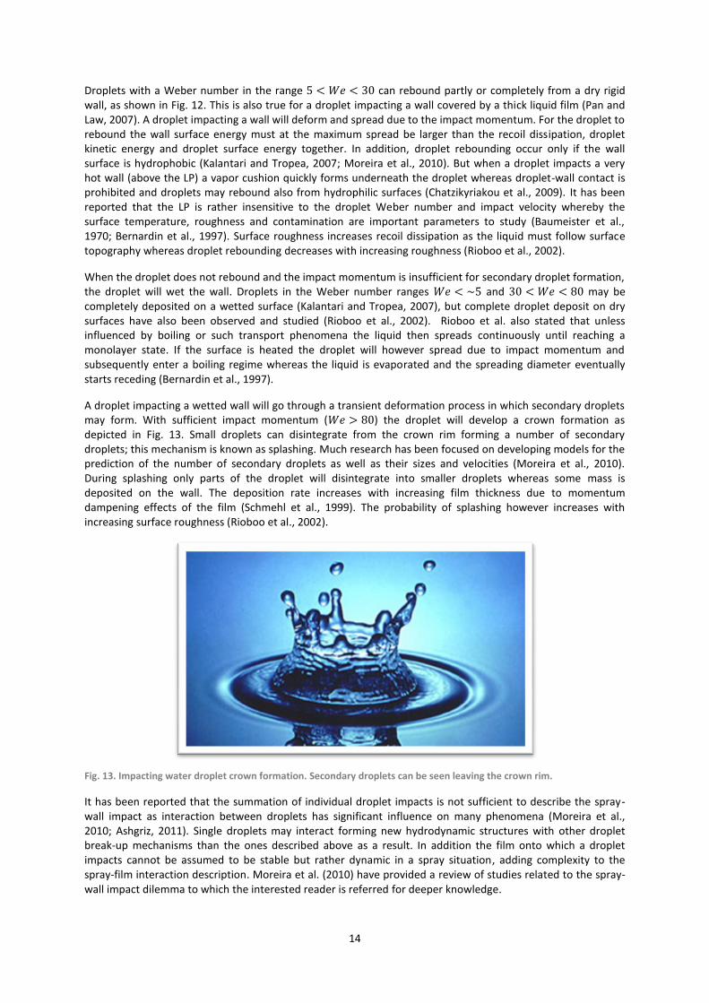
A droplet impacting a wetted wall will go through a transient deformation process in which secondary droplets may form. With sufficient impact momentum ( ) the droplet will develop a crown formation as depicted in Fig. 13. Small droplets can disintegrate from the crown rim forming a number of secondary droplets; this mechanism is known as splashing. Much research has been focused on developing models for the prediction of the number of secondary droplets as well as their sizes and velocities (Moreira et al., 2010). During splashing only parts of the droplet will disintegrate into smaller droplets whereas some mass is deposited on the wall. The deposition rate increases with increasing film thickness due to momentum dampening effects of the film (Schmehl et al., 1999). The probability of splashing however increases with increasing surface roughness (Rioboo et al., 2002).

Fig. 13. Impacting water droplet crown formation. Secondary droplets can be seen leaving the crown rim.

It has been reported that the summation of individual droplet impacts is not sufficient to describe the spray-wall impact as interaction between droplets has significant influence on many phenomena (Moreira et al., 2010; Ashgriz, 2011). Single droplets may interact forming new hydrodynamic structures with other droplet break-up mechanisms than the ones described above as a result. In addition the film onto which a droplet impacts cannot be assumed to be stable but rather dynamic in a spray situation, adding complexity to the spray-film interaction description. Moreira et al. (2010) have provided a review of studies related to the spray-wall impact dilemma to which the interested reader is referred for deeper knowledge.

15

3.2 Computational Fluid Dynamics Modeling When modeling a flow situation, partial differential equations are used to describe transport of momentum, heat and mass. These equations are difficult to solve analytically whereas they must be solved numerically. CFD is a method in which the geometry is divided into sufficient number of computational cells in order to rewrite the differential equations as algebraic equations in each cell. Thus CFD allows detailed simulation of flow combined with heat and mass transfer. Additional models such as turbulence, multiphase and mixing models can be added to expand the area of CFD applications (Andersson et al., 2012). This section will introduce important theoretical aspects of CFD that are relevant for this thesis.

3.2.1 Geometry and Meshing The basis of a CFD simulation is the geometry of the considered system. The geometry is generally drawn in a CAD program and can be one-dimensional, two-dimensional or three-dimensional. When the geometry has been drawn it is divided into smaller sub-geometries or a mesh using meshing software. The drawing cannot be too detailed since that would introduce too many computational cells during meshing. Meshing is generally a trade-off between introducing more computational cells to increase accuracy and fewer cells to decrease computational times.

3.2.2 Governing Equations To perform a CFD simulation the transport equations describing the flow are solved. These equations include: equation of continuity, Navier-Stokes equations, energy equation and species equations. These are coupled partial differential equations and described further below.

Equation of Continuity The equation of continuity, Eq. (1), is derived from the material balance over a fluid element.

(1)

At velocities limited to roughly one third of the speed of sound, the flow can be assumed incompressible. This is due to that pressure waves are spread with the speed of sound and the variation of density due to these waves can thus be neglected (Andersson et al., 2012). The equation of continuity is greatly simplified by this assumption, Eq. (2).

(2)

Navier-Stokes Equations (Momentum Equations) The Navier-Stokes equations, Eq. (3), are derived from the momentum balance over a fluid element. It can provide information of velocity variation and pressure gradients in numerous flow situations (Welty et al., 2008).

(3)

The second term on the right hand side is a simplification of the stress term based on the assumption of a Newtonian fluid. The last term on the right hand side is a gravity term.

Energy Equation The total energy equation is given in Eq. (4), where as defined in Eq. (5), is the diffusional flux of species A. The equation is derived from kinetic, thermal, chemical- and potential energy balances over a fluid element (Andersson et al., 2012).

(4)

(5)

Assuming incompressible flow the kinetic, thermal and chemical energy equations can be written separately. The balance for kinetic energy is then derived from momentum equations and the balance for thermal energy

16

is derived from the transport equation of heat and chemical reaction source terms. The transformation between kinetic and thermal energy are accounted for as source terms in their respective equations.

Species Equations The species equation, Eq. (6), accounts for transport and reaction of species in incompressible fluids. It is derived from the species balance over a fluid element where chemical reactions are accounted for by a source term.

(6)

3.2.3 Numerical Aspects During CFD simulations the governing equations are solved iteratively in each cell by approximating the partial differential equations as algebraic equations. In order to reach a stable converging solution one must consider the numerical aspects of calculations. Thus the choice of correct numerical schemes and solvers are of importance.

Numerical Scheme The governing equations are typically solved using cell face values whilst it is the cell value that is known. alues of cell’s faces are thus interpolated from values at the center of the cell itself and neighboring cells. The procedure of interpolation may have significant effects on the results of simulations.

Calculations of convective flows require extra attention. The information provided during calculation needs to be transported in the same direction as the flow to ensure a correct and stable solution (Andersson et al., 2012). Discretization schemes where information is taken from upwind cells have been developed for this reason. The most common upwind schemes are the 1

st and 2

nd order upwind schemes but there are also others

such as the QUICK scheme.

The 1st

order scheme uses information from one upwind cell whilst the 2nd

order scheme uses information from two. The 1

st order scheme is bounded which increases stability and robustness. The 2

nd order scheme is

unbounded but is instead more accurate. The accuracy originates from the Taylor expansion approximation where the Lagrange remainder of the 2

nd order scheme is of higher order than that of the 1

st order scheme

(Andersson et al., 2012). Higher order discretization schemes will be even more accurate but less robust leading to a compromise between accuracy and stability. Simulation is often started using the 1

st order scheme

to obtain a first rough solution and then switched to 2nd

order scheme to enhance accuracy. The Quadratic Upstream Interpolation for Convective Kinetics (QUICK) scheme uses quadratic interpolation of three upstream points whereas its Lagrange remainder is of 3

rd order. It is better for solving swirling flows than the 2

nd order

scheme but is applicable only to hexahedral meshes (ANSYS Inc., 2011; Andersson et al., 2012).

Solvers As previously noted, solving the governing equations implies the calculation of a complex system of algebraic equations. Solving for the velocity and pressure fields requires an iterative procedure in order to avoid numerical problems. Several algorithms have been developed and are discussed briefly below.

The Semi-Implicit Method for Pressure-Linked Equations (SIMPLE) is a commonly used algorithm that uses a starting guess for pressure and velocities to solve the Navier-Stokes equations in order to calculate the velocities. Since the starting guesses are not correct, correction factors for pressure and velocity are introduced. The correction factors are determined from their own transport equations whereafter they are used to solve other transport equations (Andersson et al., 2012). There are a number of improved variants of SIMPLE such as the SIMPLER, SIMPLEC and PISO algorithms. For calculations involving swirling flow and natural convection the PRESTO! algorithm can be used. It solves the discrete continuity equation on a shifted mesh in order to calculate the pressure field (Andersson et al., 2012).

Convergence A major issue in CFD modeling is to decide when a solution is converged, and as a result there are different measures of convergence. A solution can be considered converged when steady state is reached for all parameters involved in the calculation. This is said to be achieved when no single cell changes its values more than a small threshold between two iterations. The threshold is typically defined from the normalized largest

17

deviation in one cell during the first five iterations of simulation and a user defined convergence limit (Andersson et al., 2012). The need of details in analysis must be considered when setting the convergence limit in order to obtain appropriate accuracy and calculation times. Another way of determining convergence is to monitor species or flow properties using e.g. a surface monitor of pressure. When constant levels of monitored properties are observed, this can indicate steady state convergence. When tracing particles in a multiphase flow using an Euler-Lagrange model, the number of traced particles should be monitored. When the number of particles in the system is relatively constant, this can indicate convergence. It is recommended to use a combination of different convergence criteria to obtain correct results.

3.2.4 Turbulence Modeling Turbulence is accounted for by the Navier-Stokes equations and can be solved exactly. This however requires a grid that is finer and a time step that is smaller than the smallest scales of turbulence. This way of solving turbulence exactly is referred to as direct numerical simulation (DNS) and is extremely computationally heavy. Thus to enable simulation of engineering problems several ways of modeling turbulence have been developed. Some models filter out and model the smallest turbulence scales (e.g. Large-eddy simulation) while some model all scales statistically (e.g. two-equation models) (Andersson et al., 2012).

The two-equation models are based on the Reynolds Averaged Navier-Stokes equations (RANS) which enables a statistical approach to turbulence modeling. The Navier-Stokes equations are averaged over a time scale so that the scales of turbulence are separated. Thus the variables are split into a mean part and a fluctuating part, known as Reynolds decomposition {Eq. (7) and (8)}.

(7)

(8)

The decomposed variables are entered into the Navier-Stokes equations resulting in the RANS equations, Eq. (9).

(9)

The RANS equations introduce the Reynolds stresses {last term on the right hand side of Eq. (9)} that must be closed when solving the equations. The closure is done by using the Boussinesq approximation to model the Reynolds stresses, Eq. (10). The Boussinesq approximation is based on the assumptions that the Reynolds stresses are proportional to the mean velocity gradients and thus eddies behave like molecules, turbulence is isotropic and that there is equilibrium between stress and strain. Thus the models based on the Boussinesq equation are limited to predicting isotropic flows in local equilibrium (Andersson et al., 2012). The Boussinesq approximation also assumes that turbulent transport of momentum is diffusive and that the Reynolds stresses can be modeled by a turbulent or eddy viscosity ( ). The turbulent viscosity is a property of the turbulent flow and is defined in Eq. (11), where and are the characteristic length and time scales of turbulence respectively. The same in itself is modeled, for instance with and when using a k-ɛ model.

(10)

(11)

Standard k-ɛ Model The k-ɛ models are based on the turbulent kinetic energy ( ) and the energy dissipation rate ( ) being determined from their own transport equations. For the standard k-ɛ model the transport equations for and are given in Eqs. (12) and (13) respectively.

(12)

18

(13)

There are several terms that must be modeled in order to close the equations. The closures are done using the

variables , and

. The standard k-ɛ model is rather robust but cannot accurately predict complex flows

such as streamline curvature, swirling flows, axisymmetric jets and low Reynolds number regions (Andersson et al., 2012). This originates from the limitations of the Boussinesq approximation.

Realizable k-ɛ Model The realizable k-ɛ model differs from the standard k-ɛ model in that there is a realizability constraint on the predicted stress tensor. For flows with large strain rates the predicted normal stresses can become negative, see Eq. (14), which is not in compliance with its definition (sum of squares). The realizable k-ɛ model uses a variable to ensure that the normal stress terms are always positive, Eq. (15).

(14)

(15)

The realizable k-ɛ model fulfills Schwarz’s inequality, Eq. (16), and can thus better handle flows involving separation and rotation (Andersson et al., 2012).

(16)

SST k-ω Model The k-ω model is based on the turbulent kinetic energy ( ) and the specific dissipation rate (ω) being determined from their own transport equations. For the k-ω model the transport equations for and ω are given in Eqs. (17) and (18) respectively.

(17)

(18)

The k-ω model can handle flow in low Reynolds number regions more accurately than the k-ɛ models since the specific dissipation rate instead of the dissipation rate is modeled, thus there is no need for wall functions. On the other hand, the near wall mesh needs to be finer when using the k-ω model. The model can give good predictions when there are boundary layers with constant pressure and with adverse pressure gradients (Andersson et al., 2012).

A modification of the standard k-ω model is the Shear-Stress Transport (SST) k-ω model. This model combines the advantages of the k-ω and k-ɛ models by introducing a blending function. The SST k-ω model employs the k-ω formulation near-walls, the k-ɛ formulation in the free stream and a blend of the two in between (ANSYS Inc., 2011). Thus the near wall mesh still needs to be fine since no wall functions are used.

y+ and Wall Functions In near wall regions there are boundary sub-layers where different kinds of viscosity dominate momentum transfer as previously described. To determine the physical extent of these layers one can introduce the scaled variable , Eq. (19). This variable relates the distance from the wall to the characteristic length ( ) and velocity ( ) of the system.

(19)

The contribution of the viscous and Reynolds stresses can visualize the extent of near wall sub-layers as in Fig. 14. The viscous sub-layer is dominant when , buffer sub-layer when and the fully turbulent sub-layer when (Andersson et al., 2012). Thus when using a k-ω turbulence model

19

the first grid point should be in the range of but as close to one as possible. Wall functions (described below) should only model the viscous and buffer sub-layers whereas it is recommended to have in the first cell grid point.

Fig. 14. The extent of near wall sub-layers with Y+ (Andersson et al., 2012). Molecular viscosity is dominant near the wall and eddy viscosity is increasingly dominant further from the wall.

Many turbulence models such as the k-ɛ models are not suitable to use in regions of low Reynolds number, thus these areas must be modeled. This is done using wall functions meaning that boundary conditions are applied some distance from the wall in order to prevent the turbulence model to be solved near the wall where molecular viscosity is dominant. Standard wall functions assume there is local equilibrium between turbulence production and dissipation and the variables being modeled are the mean velocity and near wall turbulence quantities (k and ɛ or Reynolds stresses). When the local equilibrium assumption cannot be justified, for instance when there is flow separation, the use of standard wall functions is inappropriate. To account for the effects of flow separation non-equilibrium wall functions can be used, they are sensitized to pressure gradient effects through relaxation of equilibrium conditions (Andersson et al., 2012).

3.2.5 Multiphase Modeling Many kinds of flows can be classified as multiphase flows. There are mixture flows of the different phases (gas/liquid/solid) but also two immiscible liquids can be defined as a multiphase flow. It is important to determine whether the phases present are separated or dispersed. In a separated flow, the phases are quite separated with few interfaces. In a dispersed flow, one phase is present as particles or droplets meaning that there are many small interfaces. Several multiphase models have been developed to account for dispersed/separated flows, particle/droplet flows etc. The multiphase model of choice is thus dependent on the specific situation, some common models with their strengths and weaknesses are described below.

Discrete Particle Method The discrete particle method (DPM) or the Eularian-Lagrangian method is used to model a dispersed phase in a continuous phase fluid. The fluid is solved as a continuum through the normal governing equations. The dispersed phase consists of numerous particles that are traced by determining the forces acting on each particle (see below), and where the phases can exchange momentum, heat and mass with each other. DPM models are limited to systems with a low volume fraction of dispersed phase and the particles have to be much smaller than the grid cells (Andersson et al., 2012).

Forces on Particles Originating from Newton’s second law, the forces acting on a single particle are seen on the right hand side of Eq. (20) and explained in consecutive order below. A force balance taking the appropriate forces into consideration is used by FLUENT to calculate droplet trajectories and momentum exchange with the continuous phase (ANSYS Inc., 2011).

(20)

1. - The drag force acting on the particle. It is determined from the relative velocity between the

continuous phase and particle, the particle’s projected area in the flow direction and the drag coefficient compensating for non-spherical geometry.

20

2. - Pressure and shear forces from the continuous phase acting on the particle. It is determined by

the pressure and shear gradient over the particle surface. 3. - The virtual mass force acting on the particle. Virtual mass is the apparent mass of the particle in

cases of relative acceleration or deceleration between the particle and surrounding fluid. This force can be neglected when the density of the fluid is much lower than the density of the particle.

4. - The history forces acting on the particle. It arises from the development of a boundary layer

over time as the particle accelerates or decelerates. This force can be neglected when the density of the fluid is much lower than the density of the particle.

5. - The buoyancy force acting on the particle. It is the result of the density difference between the

particle and continuous phase (Archimedes’ principle). 6. - The lift force acting on the particle. It is the result of velocity being higher on one side of the

particle. This force can be neglected when the density of the fluid is much lower than the density of the particle.

7. - The thermophoretic force acting on the particle. It is a result of temperature gradients in the

fluid and is only significant for very small particles. 8. - The force resulting from turbulence acting on the particle. It is modeled as a random addition to

continuous phase velocity that lasts for the minimum lifetime of the turbulent eddy and the time taken for the particle to pass through the eddy. This force can be neglected when the density of the fluid is much lower than the density of the particle.

9. - The Brownian force acting on the particle. It results from random collisions of molecules and can

be modeled as white noise, but is only significant for very small particles.

Particle Heat and Mass Transfer Particles are in the DPM framework assumed to be perfectly spherical and with a homogenous internal temperature whereas internal transport phenomena are neglected. For dispersed droplets with a single volatile component FLUENT can apply three laws of heat and mass transfer: inert heating or cooling, droplet vaporization and droplet boiling. The law under which the particle obeys is determined by its temperature. A vaporization temperature at which slow evaporation is assumed to begin and a saturation temperature at which boiling commences must be specified by the user.

Below the vaporization temperature the particle will obey the inert heating or cooling law where there is no interfacial mass transfer whereas only heat transfer will be calculated. Heat transfer is determined by standard mechanisms as described in Transport Phenomena above. In between the vaporization and saturation temperatures the particle obeys under the droplet vaporization law. Interfacial mass transfer is here either governed by diffusion or convection/diffusion, mechanisms also presented under Transport Phenomena above. The vaporized mass will be added as a source term to the continuous phase. Heat transfer is described as in the previous law but with a source term taking the heat of vaporization into consideration. At the saturation temperature the particle will enter the droplet boiling law at which its temperature will remain at the same temperature until it is fully evaporated. The boiling model considers convective mass transfer, the same heat transfer as previous model but will in addition calculate a boiling rate transport equation solving for the droplet diameter.

Particle-Wall Interaction Models A particle with sufficient momentum might impact a wall boundary. FLUENT has four in built models to account for discrete particle and wall interaction, namely the reflect, trap, wall-film and wall-jet models (ANSYS Inc., 2011). A description of each is given below, with emphasis on the wall-film model since it is of extra importance to this thesis.

The reflect boundary condition is fairly simple. Particles impacting a wall will rebound and retain some of its momentum. The user can specify the degree of momentum and energy losses of the impact through two factors of restitution, that of velocity magnitude and that of the impact angle. This boundary condition corresponds to the expected droplet behavior at wall impact above the Leidenfrost temperature.

The trap boundary condition is even easier to describe numerically, it does not however correspond to any physical mechanisms. As a particle encounters a wall its trajectory tracing is terminated and the particle mass is removed. The volatile part of its mass is added to the vapor phase in the cell nearest the wall and the enthalpy of vaporization is taken from that same cell.

21

The wall-film model contains a more complex framework than the above boundary conditions. At droplet impact there are four possible events: stick, spread, splash or rebound. The criteria for the interactions are set by the wall temperature and the impact energy of the impacting droplet, where the kinetic energy is a function of the particle Weber number. During the sticking regime the particle velocity is simply set to the wall velocity. In the spreading regime the impact velocity and direction are used to determine the spreading of the droplet across the wall. The splash regimes tries to describe the secondary atomization as previously described in Droplet-Wall Interaction. The number of particles created by a splash can be specified and the size and velocity of these are randomly calculated from an experimentally determined distribution. In the rebound regime the droplet will behave similarly to the reflect boundary condition.

The wall-film particle velocity along the wall is governed by a momentum transport equation where shear stress, pressure gradient etc. is taken into account. Mass transfer from the film is governed by Eq. (21) where is determined through a correlation of the Reynolds and Schmidt numbers and where the concentration gradient is that between the film surface and gas phase. The film heat transfer is determined through a heat transport equation taking both conduction and convection into account. Heat from the wall is assumed to be limited by liquid conduction. There is a source term for the latent heat of the evaporating mass, the enthalpy of vaporization is however subtracted from the cell to which the vapor mass goes. During high rates of evaporation, the heat of vaporization exceeds the heat transfer from the wall. In addition the wall heat flux to the wall-film is subtracted from the wall heat flux to the gaseous phase (ANSYS Inc., 2011). Obviously the heat flux will be negative when wall-film coverage is dense. This can lead to deceptive wall heat fluxes and unrealistic cooling of the cells near the walls.

(21)

In the wall-jet model droplets will either rebound or stick. The model is suitable when the wall is very hot (above the Leidenfrost temperature) and film formation is not occurring. The rebound velocity and direction is determined as a function of the impact angle and the droplet Weber number. The function determining this is an analogy with an inviscid jet impacting a solid wall (ANSYS Inc., 2011). Particle heat and mass transfer are then determined by above described Particle Heat and Mass Transfer.

Eularian-Eularian Method The Eularian-Eularian method is used to model multiphase flow although it can also be used to model two immiscible liquids. Each phase is modeled as though being continuous and solved for through the governing equations previously presented. The phases can exchange momentum, heat and mass with each other, see for instance the description of the Rensselaer Polytechnic Institute (RPI) boiling model below. A standard Eularian-Eularian model does not track the interface between phases whereas the volume of fluid model (VOF) should be utilized if this is of interest.

RPI Boiling Model The RPI model is developed for a Eularian-Eularian modeling approach to sub-cooled flow nucleate boiling applications. The fundamental assumption of the model is that heat transfer can be described by three mechanisms: convective heat flux, quenching heat flux and evaporative heat flux as given in Eq. (22).

(22)

Having been developed for flow boiling it is assumed that there is a liquid bulk that covers the wall surface except where nucleating bubbles appear. Thus there is a normalized surface area assumed to be covered by the nucleating bubbles and an area covered by liquid. This parameter is used to determine the area of influence of the stated heat mechanisms and its closure can be modeled as in Eq. (23) (ANSYS Inc., 2011).

(23)

In the above equation is the nucleate site density, the bubble departure diameter and an empirical constant. The interested reader is referred to Del Valle and Kenning (1985) for further discussion on this empirical constant.

The convective term is the heat transferred from the wall to the liquid through single phase convection as given in Eq. (24).

(24)

22

Where is the convective heat transfer coefficient and where and are the temperatures of the wall

and liquid respectively. The heat transfer coefficient is calculated through the local Nusselt number.

The quenching term is the heat transfer resulting from liquid filling the void when a bubble detaches from the wall and is calculated according to Eq. (25).

(25)

Where and are the liquid thermal conductivity and diffusivity respectively and the periodic time of bubble detachment.

The evaporative term is the heat transferred from the wall to fuel vaporization in bubble growth and is given by Eq. (26).

(26)

Where is the volume of the bubble, the nucleation site density, and the bubble departure frequency.

The heat flux equations stated above need closures for the bubble departure diameter (used to determine the volume of departing bubbles), the nucleation site density, and the bubble departure frequency. There are several closures for the bubble departure diameters, nucleation site density and bubble departure frequency incorporated into FLUENT to choose from. The interested reader is referred to the FLUENT manual (ANSYS Inc., 2011).

As mentioned in Nucleate Boiling the surface structure at which boiling occurs is along with other system properties of great importance and the modeled variables above are all affected. Since the influence of these closures on simulation results is substantial they must be tuned to match experimental data. Especially the bubble departure diameter is of great importance as it relates to the heat flux according to Eq. (27).

(27)

As mentioned above the model is developed for the application of sub-cooled flow boiling and does thus include description of bubble condensation as it reaches the sub-cooled bulk. After personal communication with model co-developer Professor Michael Podowski at the Rensselaer Polytechnic Institute on September 19

th, 2012 it was concluded that the model is not directly applicable to the dispersed droplet boiling problem

faced in this thesis. It should however be possible to modify the physical description of nucleate boiling included in the RPI model to suit the problem on hand.

Mixture Model The mixture model is used to model multiphase flow by solving one set of previously described governing equations for the mixture. The relative velocity between the modeled phases are then determined through an algebraic slip expression. The main assumption is that local equilibrium between phase velocities is reached over a short spatial length scale (ANSYS Inc., 2011). To model phase transition the evaporation-condensation model is available within the mixture model framework.

Evaporation-Condensation Model The evaporation-condensation model describes the phase transition between liquid and vapor by calculating the vapor transport equation. The rates of evaporation and condensation are determined by the difference between the operating and saturation temperatures as well as a user set coefficient. The coefficient should be specified so as to fit to case specific empirical data (ANSYS Inc., 2011).

3.2.6 Boundary Conditions Boundary conditions are of great importance in CFD modeling. Inlet conditions specify the input into the system while outlet conditions affect what exits the system. Wall boundaries are important as they may interact strongly with the flow and to start simulations initial conditions must be specified. These aspects of CFD modeling are discussed below.

Inlet Conditions Inlet conditions can be set by for instance flow velocity or mass flow rate. The state of the fluid, such as the temperature and density, entering the system is also specified. Inlet conditions are however often quite unphysical as boundary layers are not present in the inlet but developed after some distance into the

23

geometry. This is especially true when using certain turbulence models as the presence of turbulent boundary sub-layers are important for wall functions to work correctly. Turbulence inlet conditions can be set by for instance specifying the turbulence intensity and length scale. These can be estimated through the Reynolds number and inlet dimension. To investigate the impact of inlet conditions one can calculate how far into the system the inlet conditions survive.

Outlet Conditions The standard outlet condition is the zero-diffusion flux at outflow cells meaning that the outlet does not affect upwind cells. It is common to define a static pressure at the outlet, referred to as simulation using a pressure outlet. In such cases the normal gradient of all variables except pressure are assumed to be zero. Outlet conditions will not have the same impact on simulations as inlet conditions but problems with reverse flow may arise. Reverse flow properties must then be specified prior to simulation.

Wall Boundaries The general assumptions at wall boundaries are the no-slip condition (previously described) and the no-penetration condition which means that there is no diffusion or reaction at walls. The no-slip condition is sometimes not sufficient and complementing models must be introduced. For turbulent conditions at high Reynolds numbers, wall functions are used to model the fluid wall interaction. For particle modeling the no-slip condition might be inappropriate whereas particle wall interaction must be modeled, e.g. the wall-film model (refer back to Particle-Wall Interaction Models above). Heat transfer can be specified in several ways at wall boundaries, one can for instance specify a fixed heat flux or a fixed surface temperature.

Initial Conditions The solvers described above require an initial guess to start iterations. A commonly used guess is that conditions are the same as the specified inlet conditions. A guess that is closer to the actual solution will lead to faster convergence while a poor guess might lead to divergence. Sometimes there are multiple stationary solutions to a problem. Thus it might of interest to try different initial conditions to see if the converged solutions are the same. When performing transient simulations, the actual initial conditions need to be specified. The starting guess could then be obtained from a steady state simulation of the same problem.

Symmetrical Boundary Conditions To reduce computational times the modeled geometry can be divided into several symmetrical sub geometries. The most common symmetrical boundary condition is the mirror plane. This essentially means that all conditions are identical on both sides of the symmetrical boundary and properties transported to and through that boundary or mirror plane will thus rebound back. Another symmetrical boundary condition is the cylindrical symmetry condition. This is employed when for instance a cylinder is divided into several identical slices. Properties transported to and through one boundary will be transported into the opposite corresponding boundary. The symmetrical sub-geometries can then be assembled into the whole modeled geometry.

24

4. METHOD This section describes the procedure of conducting the CFD analysis. It is divided into four parts namely hand calculations, geometry, meshing and simulation setup.

4.1 Hand Calculations Before initiating the CFD analysis, some general hand calculations were conducted. The purpose of the same was to investigate and understand important system characteristic, but also to obtain crude approximations to check simulation validity. The hand calculations were based on process specifications obtained from Getinge Skärhamn and general material data. The calculations were divided into the two sections namely steam generator and sterilization chamber and are presented in Appendix 5.

4.2 Geometry To enable a CFD-analysis, the fluid volume of concern for the simulations must be defined or constructed. While using ANSYS FLUENT the geometry model can be treated using the Design Modeler (DM) software. DM is a CAD-program and is compatible with most CAD-formats whereby external CAD-models can be imported and used to define the geometry. Often in CFD applications, only the product CAD-models are available whereas the fluid cavity must be extracted. CAD-models of the autoclave were available and obtained from Getinge Skärhamn. The models were imported into DM using the parasolid file format (*.x_t). Two different geometries, the steam generator and the sterilization chamber, were isolated and treated further as described below.

4.2.1 Steam Generator

Steam Channel As previously stated, the CAD-model obtained from Getinge Skärhamn was imported into DM. For the initial simulations only the steam channel within the steam generator is of interest. To obtain the fluid volume (steam channel cavity), the Fill tool was used. This tool creates a volume as it fills the cavity inside a set of defined surfaces. At closer inspection of the obtained fluid volume it was discovered that there were some gaps in the original CAD-model. The correctness and validity of the CAD-models and dimensions were discussed with Getinge Skärhamn. Since the steam channel geometry is quite simple, it was instead constructed manually aided by construction dimensions obtained from Getinge Skärhamn. One half of the final constructed steam channel geometry is depicted in Fig. 15.

Fig. 15. The isolated steam channel of the steam generator. Part of the top left surface after the 90 degree bend is the outlet while an injector is placed in the bottom right of the geometry.

Part of Steam Channel Some simulations were performed in order to investigate the liquid-wall interaction close to the spray injector. In order to increase convergence times the steam channel was shortened substantially and split in two symmetrical halves through slice operations. This resulted in a long half cylinder, Fig. 16.

25

Fig. 16. The part of the steam channel used for qualitative droplet-wall interaction assessment.

4.2.2 Sterilization Chamber The sterilization chamber geometry is complex in comparison with the steam channel. The product CAD-model was imported into DM. Small details such as screws and bolts were removed using the Face delete tool as these are impractical in CFD-simulations. The model was comprised by many small assembled components, thus the Fill tool was inapplicable when defining the chamber cavity as a fluid volume. Instead the Enclosure tool which encloses the whole CAD-model with a volume was used. A Boolean subtraction operation was then performed yielding the fluid volume as well as some unwanted volumes that were suppressed. To obtain the final sterilization chamber geometry the inlet part of the chamber was sliced where the inlet plate is attached.

During sterilization the chamber is not empty but loaded with trays. The trays were simplified to hollow rectangular boxes with steam openings. The hollow boxes were manually constructed and then separated from the chamber volume using a Boolean operation. The tray walls were needed for heat transfer calculations whereas they were defined as aluminum. The loaded sterilization chamber geometry is shown in Fig. 17.

Fig. 17. The sterilization chamber with trays. The left hand figure highlights the trays. The right hand side shows the sterilization chamber having been sliced to enable sweep meshing.

26

In addition, a simplified geometry was used to investigate the feasibility of modeling high rates of condensation. The same was simply comprised of two cubical parts being defined as solid and fluid volumes respectively.

4.3 Meshing The geometries edited in DM were imported into the ANSYS mesh software Meshing (M). Both geometries, steam generator and sterilization chamber, were sliced into two symmetrical halves in order to reduce the number of cells and thus reduce computational times. The steam generator and sterilization chamber geometries did however require different treatment during meshing and the process of each case is described below.


Steam Channel The geometry consists of a long cylinder channel and a 90° bend. To enable different meshing methods on the two parts, the geometry was divided into two parts (the slice is visible in Fig. 15). The cylinder channel part has a uniform cross sectional area whereas it is possible to use the sweep meshing method. By using the sweeping method the mesh will be swept from the start to the end surface. This means that there will be no tetrahedral but merely pentahedral and hexahedral cells. Thus the number of cells is reduced and the cell quality with respect to tangential flow increased. The bend part of the geometry is not applicable for sweep meshing whereas it will be comprised by tetrahedrons. Near-wall regions require a finer mesh whereas cell inflation was used. Appropriate mesh size was determined from dimensionless number analysis in Appendix 5 and inflation parameters were tuned with respect to from initial single phase simulations. The quality of the mesh was investigated by looking at mesh metrics such as element quality, aspect ratio, skewness etc. Mesh size, inflation parameters and mesh metrics are presented in the Appendix 6. The mesh used is shown in Fig. 18.

Fig. 18. Mesh of the full steam channel. The left hand figure is a close up of the 90 degree bend where the interface between the sweep mesh and tetrahedral mesh is. The right hand figure depicts the surface at the beginning of the steam channel. By examining the near wall areas one can see the inflation introduced in the mesh.

Part of Steam Channel The part of the steam channel as described above is constituted by a simple cylinder, thus sweep meshing was utilized for the whole domain. To be able to resolve all desired phenomena the density of the mesh was high. In addition, inflation was used near the wall so as to resolve the droplet-wall interaction. The mesh is shown in Fig. 19.

27

Fig. 19. Mesh of the part of the steam channel. The mesh is finer than that of the full geometry enabling qualitative analysis of important system characteristics.

4.3.2 Sterilization Chamber The mesh for the sterilization chamber is shown in Fig. 20. The sterilization chamber geometry is quite complex in comparison with the steam channel. It was not possible to sweep the whole domain whereas the geometry was split into several zones. A tetrahedral mesh was used in zones where sweeping was not possible. Since some turbulence was expected cell inflation was used in near-wall regions. Appropriate mesh size was determined from dimensional number analysis by hand calculations in Appendix 5 and from initial simulations. The quality of the mesh was determined by examining mesh metrics as stated above, results are presented in Appendix 6.

Fig. 20. Mesh of the sterilization chamber. The chamber was split to enable as much sweep meshing as possible. There is inflation near the chamber’s outer walls and a fine mesh near the tray walls.

The meshes of the simplified geometries used during modeling of condensation are shown in Fig. 21. In the simplest case, only two computational cells were included. The number of cells was then increased, yielding 128 perfectly orthogonal cells (left part in Fig. 21).

28

Fig. 21. Meshes of the simplified geometry used in condensation modeling. Left: Cubical fluid and solid volumes each split into 64 perfect computational cells. Right: Cubical fluid and solid volumes each comprised of one orthogonal computational cell.

4.4 Simulation Setup This section describes the simulation setups applied in ANSYS FLUENT, it is divided into descriptions of the steam generator and sterilization chamber simulations. Each simulation setup will be discussed considering model selection, material properties, boundary conditions and solution aspects.


Single Phase Simulations: Choice of Turbulence Model The initial simulations were performed under simplified single phase conditions where a steady state solution was sought after. During this stage no particles were injected whereas only steam was assumed to flow through the system. The operation pressure varies between but was here for simplicity assumed to be steady at .

Models In the first simulation no turbulence model was chosen whereas the flow was modeled as though being laminar. When the basic flow characteristics of the system had been investigated the standard k-ɛ, realizable k-ɛ and the SST k-ω turbulence models were tested since previous calculations of the cylinder flow Reynolds number had indicated a turbulent system. The modeled geometry consists of a bend where flow separation was expected. The k-ɛ models require the use of wall-functions whereas standard and non-equilibrium wall-functions were tested for both models due to the expected flow separation at the bend. Since some areas of the geometry were later during multiphase flow expected to have slightly lower Reynolds numbers the SST k-ω model was also tested. The SST k-ω model requires a denser mesh near the walls than do the k-ɛ models whereas mesh density was increased prior to this simulation.

Materials As previously mentioned pure steam was assumed to flow through the Steam Channel. FLUENT’s default steam data was used as it is valid at a pressure of . Thermal properties of steam were not considered during these simulations.

Boundary Conditions The inlet boundary conditions were determined from the mass flow rate and initially no velocity profile was defined. When turbulence models were tested, a turbulent velocity profile was used. The profile was generated by copying the velocity profile over a Steam Channel cross-section surface some distance into the geometry and using it as inlet velocity profile in the next simulation. This procedure was repeated to obtain a fully developed turbulent velocity profile as an inlet boundary condition. The obtained velocity profile will not be of any use during multiphase simulations but merely when analyzing the choice of turbulence model. The no-slip wall boundary condition was applied and thermal boundary conditions were at this stage not set. The outlet was defined as a pressure-outlet with no gauge pressure.

29

Solution The SIMPLE scheme was used for pressure-velocity coupling calculations. During the first iterations of each simulation, a 1

st order discretization scheme was used for all quantities. To avoid numerical diffusion, 2

nd order

discretization was applied as soon as the 1st

order solution had converged slightly giving increased solution accuracy. The default under-relaxation factors (URF) were not altered unless residuals were high during simulation. The initialization values were taken from the inlet. The scaled residuals were plotted until having reached below the threshold value in order to measure convergence. In addition velocity, pressure and turbulence quantities of the system were plotted and observed until stabilized as an extra convergence criterion. The final convergence measure was that for mesh independency, it was checked by performing several gradient adaptations and running the simulation a bit further.

Discrete Particle Method: Selection of Boundary Conditions The first DPM simulations were performed in a long cylinder geometry (part of original steam channel) in order to evaluate heat transfer and particle wall interaction with fast convergence. The operation pressure varies between but was here for simplicity assumed to be steady at since a steady state solution was desired.

Models The DPM model was enabled and run with a transient simulation for both the continuous flow and particle tracking. At first, particles with uniform diameter ( ) were injected to simplify modeling of the system. Basic mechanisms of heat and mass transfer were investigated, especially in the near wall regions. Thereafter, the droplet diameter was assumed to be Rosin-Rammler distributed between and with a spread

factor of . The spray angle was assumed to be and initial droplet velocity magnitude to be

. To

capture significant events, a particle trajectory calculation time step of was used. To ensure a sufficient coupling between the phases the DPM sources were updated after every continuous phase iteration as well as making one particle trajectory calculation after every continuous flow time step. In addition the DPM URF was kept as high as possible.

To include evaporation of the droplets, the energy equation was enabled. During the first iterations a k-ɛ turbulence model was used to in order quickly obtain a rough approximation of the flow situation. After a while the k-ω SST model was switched on as it also accounts for low-Reynolds number regions and thus increases the accuracy under these circumstances.

Materials The materials needed to be specified in the simulations were liquid water and steam. FLUENT’s default liquid water and steam data were used during simulations as it is valid at a pressure of .

Boundary Conditions All boundaries enclosing the fluid volume except the outlet were defined as walls since the droplet injector is the geometry’s only inlet. The inlet conditions of the droplet injector were described under the Models heading above, and the wall temperature was fixed at . The DPM model needs extra treatment to handle particle-wall interaction and FLUENT has built in models for this (see Theoretical Framework). The wall-film model was used and the number of splashed droplets at high Weber number droplet impact was assumed to be four. In addition, the wall-jet, trap and reflect models were also examined and tested. The no-slip wall boundary condition was enabled but surface roughness was not taken into consideration. The outlet was for the fluid steady state simulations defined as a pressure-outlet with no gauge pressure.

Solution The SIMPLE scheme was used for pressure-velocity coupling calculations. A 2

nd order discretization was applied

giving increased solution accuracy as compared to 1st

order discretization. The default URFs were not altered unless residuals were high during simulation. The scaled residuals were plotted and observed as not to fluctuate too much. In addition, velocity, temperature, pressure, and DPM sources conditions of the system were plotted and observed until stabilized as another convergence criterion. The number of tracked particles was monitored until reaching a fairly constant level. The final convergence measure was that for mesh independency, it was checked by considering mesh size and performing different gradient adaptations.

30

Discrete Particle Method: Full Steam Channel The purpose of these simulations was to investigate the appropriateness of the selected wall-film model and simulation setups when simulating the full steam generator geometry. At first, FLUENT default fluid properties were used but then fluid properties were assumed so as to tune simulation results to actual data obtained from Getinge Skärhamn. Model choices and simulation setups are motivated below and all results are presented in the results section.

Models The SST k-ω model was used for turbulence modeling. As previously presented, information from the hollow cone spray nozzle manufacturer was retrieved and the droplets were assumed to range between , have a mean diameter of and the cone angle to be roughly . The Rosin-Ramler distribution spread factor was assumed to be . The number of particle streams was set to for the whole geometry, and with 10 different diameters the total number of particles being injected in each time step was 200. The injector was placed into the geometry from the inlet and was assumed to have a radius of . For the unsteady particle tracking simulations a time step of was used to avoid particles from travelling through multiple cells each time step (see hand calculations in Appendix 5).

Materials The materials needed to be specified in the simulations were liquid water and steam. FLUENT’s default steam data was used during the first simulations as it is valid at a pressure of . However, assumed fluid properties were used in the second set of simulations. To increase the rate of evaporation and heat flux from walls the thermal conductivity and mass diffusivity of the gaseous phase were both increased by a factor 10. The liquid conductivity was increased by a factor 4. See the Discussion section for a discussion on this topic.

Boundary Conditions The surface previously used as gaseous inlet was redefined as a wall similar to the other channel walls since the droplet injector is the geometry’s only inlet. The wall temperature was fixed at since a steady state solution was sought after. The wall-film model was used for wall droplet interaction and the number of splashed droplets at high energy droplet impact was assumed to be four. The no-slip wall boundary condition was enabled but surface roughness was not taken into consideration. The outlet was for the fluid steady state simulations defined as a pressure-outlet with no gauge pressure.

Solution The SIMPLE scheme was used for pressure-velocity coupling calculations. Discretization schemes were handled the same way as in previous simulations. The URFs were maintained as high as possible while still obtaining convergence. The initialization values were arbitrary set from the expected steady state solution. The scaled residuals and characteristics of the system such as temperature, velocity, enthalpy, DPM mass source etc. were plotted and observed until stabilized as a convergence criterion. The number of tracked particles was monitored until reaching a fairly constant level. The final convergence measure was that of mesh independency, it was controlled by performing gradient adaptations and comparing solutions.

4.4.2 Sterilization Chamber

Single Phase Simulations The initial simulations were performed under simplified single phase conditions. During this stage no condensation was assumed to occur whereas only steam and air was assumed to be part of the system. The process being modeled was the addition of steam prior to sterilization or more specifically the time lapses of the pulses and main pressure increase in the chamber as presented in Process Details and in Appendix 5. During these simulations pressure varied between . Hand calculations in Appendix 5 were used to write a UDF, attached in Appendix 2, governing the inlet mass flow rate as a function of time for the main pressure increase stage. Since the first simulation was single phase, the condensed steam was not included when determining the mass flow rate.

Models

Since the pressure was expected to increase with the transient addition of mass into the chamber, floating operating pressure was used. This means that the operating absolute pressure is updated as the simulation continues, which is fundamental for the correct description of steam properties and the UDF to work properly.

31

In the first simulation no turbulence model was chosen due to the low velocities whereas the flow was modeled as though being laminar.

Materials

As previously mentioned only steam and air was assumed to be present in the Sterilization Chamber. FLUENT’s default air and steam data was examined and redefined according to data from Mörstedt and Hellsten (2008) where significant property dependence on temperature or pressure was noticed. The ideal gas law was used as equation of state since the density was expected to increase as pressure increases.

Boundary Conditions

The inlet steam was assumed to be saturated at the given operating pressure. Thus, another UDF was implemented setting the inlet temperature to the saturation temperature at the instantaneous operating absolute pressure. The UDF is attached in Appendix 2. The inlet geometry of the sterilization chamber is quite original and its velocity profile not intuitive. The inlet boundary conditions were thus determined from the mass flow rate and no velocity profile was defined. The no-slip wall boundary condition was applied and boundaries were set to be thermally isolated. The outlet was redefined as a wall since the outlet valve is closed during the modeled time lapse.

Solution A time step of was used for the transient solution in this simulation. The SIMPLE scheme was used for pressure-velocity coupling calculations. Discretization schemes were handled the same way as in previous simulations. The default URFs were not altered unless residuals were high during simulation. The initialization values such as gauge pressure and velocities were simply set to zero since this is the assumed state of the system prior to the process. The scaled residuals as well as velocity and pressure conditions of the system were plotted and observed until stabilized in each time step as a convergence criterion.

Multiphase Simulations The purpose of these simulations was to examine the feasibility of modeling high rates of condensation. A simple geometry was implemented due to the time scope of the thesis work. Two simple meshes were used to investigate the feasibility of modeling such high rates as were shown in the Meshing section above.

Models FLUENT’s built in evaporation-condensation model was utilized within the mixture multiphase model. Gravity was enabled with an acceleration constant of

. The evaporation-condensation model’s condensation

frequency parameter was tuned (=1) in order to yield a high rate of condensation. A floating operating pressure was utilized as the pressure was expected to increase with the addition of steam.

Materials Similar to the single phase simulations the ideal gas law was used as equation of state for the gaseous phase. Liquid water was however assumed to be incompressible with a constant density. Properties of steam and liquid water were examined so as to be valid in the simulation temperature and pressure ranges.

Boundary Conditions The inlet boundary conditions were determined from the mass flow rate and no velocity profile was defined. The no-slip wall boundary condition was applied. The inlet mass flow rates of the simplified simulations were set in order to reproduce the relation between the volumetric flow rate and the fluid volume in the real sterilization chamber. The initial fluid cell temperature was set to and that of the solid cell to . Heat transfer at the fluid-solid interface was set to convection and conduction, while the surrounding surfaces were assumed adiabatic.

Solution A time step of was used for the transient process. The body force weighted scheme was used for pressure-velocity coupling calculations. The QUICK discretization scheme was used for all other equations. The default URFs were not altered unless residuals were high during simulation. The initialization values such as gauge pressure and velocities were set to zero. The scaled residuals and velocity, temperature, density and pressure conditions of the system were plotted and observed until stabilized in each time step as an extra convergence criterion.

32

5. RESULTS This section includes figures, graphs and description of obtained simulation results. It is divided into the two parts, namely steam generator and sterilization chamber. Quantitative results in tabular form are presented in Appendix 6.

5.1 Steam Generator

5.1.1 Single Phase Simulations: Choice of Turbulence Model The aim of the single phase simulations was to test and select an appropriate turbulence model prior to conducting the multiphase simulations. At first the flow field was assumed laminar so as to obtain a first view of continuous phase behavior in the system. The three two-equation turbulence models standard k-ɛ, realizable k-ɛ and SST k-ω were then applied and examined. Below are some figures and description of obtained results.

Prior to reviewing results, it should be noted that the multiphase system is expected to differ significantly from the simulated single phase system. In reality the liquid spray is the only added mass and evaporation will induce the pressure increase leading to continuous phase flow. An acceleration of the continuous phase flow is therefore expected upstream and there will be regions of low velocity magnitudes near the inlet. In addition, there is a presence of stagnant area closer to the exit as shown in Fig. 22 below. One can therefore expect some low Reynolds number regions, which is an important factor to be considered while selecting a suitable turbulence model.

Fig. 22. Velocity magnitude contour near the outlet. The low velocity at the end of the steam channel clearly shown.

33

Fig. 23. Path lines colored by velocity magnitude of the single phase simulations at the outlet of the steam generator. Top left: laminar. Top right: standard k-ɛ turbulence model. Bottom left: realizable k-ɛ turbulence model. Bottom right: SST k-ω turbulence model.

The general flow field of the laminar simulation and those with the three turbulence models are quite similar, as shown in Fig. 23. Flow in the beginning of the steam channel was well structured and homogenous in all four simulations. The main difference is the stagnant area in the left part of the geometry obtained in the laminar case simulation. This will not however affect the choice of turbulence model.

Consequently it is important to consider some turbulence characteristics such as wall , turbulence kinetic energy, turbulence dissipation rate, and turbulence or eddy viscosity. An important difference between the k-ɛ and k-ω models is the near wall modeling aspect. As described in the Theoretical Framework the k- ɛ models require the use of wall functions to estimate near wall turbulence properties. The k-ω model however does not need wall functions but instead requires a finer mesh.

34

Fig. 24. contour of the turbulent single phase simulations at the outlet of the steam generator. Top left: standard k-ɛ turbulence model. Top right: realizable k-ɛ turbulence model. Bottom: SST k-ω turbulence model.

In order for the wall functions to correctly model the near wall conditions, the of the first grid point should be in the range . Looking at the contour in Fig. 24, this criterion is not quite fulfilled for both the k-ɛ turbulence models. Also to obtain a higher , with respect to k-ɛ turbulence models, one can use a coarser mesh near the wall. This is however not recommended as the mesh is already quite coarse (first grid point in from the wall), as this will increase numerical diffusion and other grid related problems. In addition, there are particle-wall interaction phenomena that need to be resolved later during multiphase simulations requiring a dense near wall mesh.

The SST k-ω model requires a of the first grid point in the range below 5. From Fig. 24, we can infer that this criterion is fulfilled in most parts of the geometry. For all three cases, the is slightly elevated in the areas near the bend due to the accelerated flow field and flow separation past the bend. From a perspective the SST k-ω model would be preferable due to the compatibility with the near wall dense mesh required for resolving important DPM phenomena during multiphase modeling.

35

The expected flow separation in the bend meant that the realizable k-ɛ model was more extensively investigated than the standard k-ɛ model as indicated in the Theoretical Framework. When the turbulent kinetic energy was considered, as shown in Fig. 25, the standard k-ɛ model was therefore excluded. Higher levels of turbulent kinetic energy can be observed in numerical results obtained from the realizable k-ɛ model compared to the SST k-ω model. There is a particular difference in the top region (near furthest to the top right) in Fig. 25, where turbulent kinetic energy is spread from the stagnant zone into other parts of the geometry. The k-ɛ models are known to overestimate turbulence in low Reynolds number regions (Andersson et al., 2012). The described region is as previously described quite stagnant whereby the Reynolds number is expected to be low. The turbulence properties are expected to be suppressed and this is not accounted for by the k-ɛ model. The SST k-ω model is therefore preferable when considering the aspect of low Reynolds number regions.

Fig. 25. Turbulent kinetic energy (k) contour of the applicable turbulence models. Left: realizable k-ɛ turbulence model. Right: SST k-ω turbulence model.

Fig. 26 shows the turbulent or eddy viscosity contours for the realizable k-ɛ and SST k-ω turbulence models. Similar to the turbulent kinetic energy, the eddy viscosity is seemingly larger for the realizable k-ɛ model. This is especially true in the regions near the stagnant zone as seen in the top right side of Fig. 26. Since less turbulence is expected in this region the eddy viscosity should be limited and not exceedingly dominant when

compared to the molecular viscosity of steam ( ). Where as In the simple channel flow, bottom left in Fig. 25 and Fig. 26, the two models behave quite similarly. The SST k-ω turbulence model is therefore suitable for multiphase simulations.

36

Fig. 26. Turbulent viscosity or eddy viscosity of the two applicable turbulence models. Left: realizable k-ɛ turbulence model. Right: SST k-ω turbulence model.

5.1.2 Discrete Particle Method: Selection of Boundary Conditions The aim of these simulations is to investigate the appropriateness of the different particle-wall interaction boundary conditions. A dense mesh was used to resolve appropriate mechanisms and make sure that temperature and concentration gradients etc. were sufficiently high. The reflect, wall-jet, wall-film and trap boundary conditions were investigated.

Reflect Boundary Condition The reflect boundary condition means that the particles simply bounce off the wall with no extra interaction treatment. From the results obtained in Fig. 27 and Fig. 28, is clearly evident that the particles simply bounce back and forth on the walls prior to exiting the geometry. The continuous phase flow field is induced by the interaction with particles which is apparent from Fig. 27. The relatively weak coupling between particle and flow momentum as determined in through hand calculations in Appendix 5 is apparent, as the particle velocity (color coded in the figure) does not decrease significantly by the slower continuous phase. In short, the velocity of the particle is much higher compared to the continuous phase.

37

Fig. 27. Velocity figure of the reflect boundary condition with injector on the right hand side of the geometry. Continuous phase velocity magnitude contour and particles colored by velocity magnitude.

The particle temperature does not increase significantly when the same hits the wall. Evidently the particle temperature will never reach the vaporization limit temperature and definitely not the saturation temperature. Hence, there is no evaporation of the particle at all. The application of reflect boundary condition is therefore not suitable for this problem where high rates of phase transition is expected. Further investigations were not conducted for this boundary condition.

Fig. 28. Temperature figure of the reflect boundary condition with injector on the right hand side of the geometry. Continuous phase temperature contour and particles colored by temperature.

38

Wall-Jet Boundary Condition As previously described in the Theoretical Framework, particles will reflect from the wall also when the wall-jet boundary condition is applied. The wall-jet model differs from the reflect boundary condition by the fact that the angle of reflection is calculated by a statistical algorithm rather than just being the angle of impact. As evident from Fig. 29, the calculated angle of reflection will induce a particle flow along the wall but not in contact with it.

Fig. 29. Velocity figure of the wall-jet boundary condition, looking into the geometry with the injector being in the opposite side of this view. Continuous phase velocity vectors and particles colored by velocity magnitude.

The same can be seen in detail from Fig. 30 where particles are sprayed on the wall and then reflected along it. This induces a strong flow current parallel to the wall. The use of the wall-jet model is not suitable for the problem on hand for other reasons. The rate of evaporation presented in Appendix 6 is very low and heat transfer to the DPM particles is limited. The model does not simulate direct contact between particles and the wall. Hence the heat transfer is only limited to gaseous phase convection or conduction.

The expected particle-wall contact boiling is not possible to model without some sort of particle impact and spreading treatment. The high rates of heat and consequently interfacial mass transfer needed for the simulation of this problem are unlikely to be reached using the wall-jet model. Further investigations of the wall-jet model is therefore not of any interest. The expected particle-wall contact boiling is not possible to model without some sort of particle impact and spreading treatment.

Fig. 30. Velocity figure of the wall-jet boundary condition, the bottom right part of the geometry with the injector being on the right hand side. Continuous phase velocity vectors and particles colored by velocity magnitude.

Wall-Film Boundary Condition The wall-film model includes four possible particle impact events, of which two can be observed in the problem on hand. Due to the particle Weber numbers and wall superheat of this specific problem the particles may either splash or reflect from the wall. When splashing, four secondary small particles leave the wall while some

39

mass is retained and spread into a wall-film across the wall. With particles reflecting, splashing and spreading across the wall, the flow field was expected to be quite complex as observed in Fig. 31. Obviously there was some reverse flow from the outlet due to the heterogeneous flow structure.

Fig. 31. Vector velocity figure of the wall-film boundary condition, particle injector on the right hand side.

The continuous phase velocity contour was overlaid with the particles colored by particle velocity in Fig. 32. From the figure it can be seen that the flow field is induced by the moving particles and we can also infer from the same, that there is insufficient evaporation of the particles.

Fig. 32. Velocity figure of the wall-film boundary condition with injector on the right hand side of the geometry. Continuous phase velocity magnitude contour and particles colored by velocity magnitude.

40

The continuous phase temperature contour and particle temperatures are shown in Fig. 33. The water particles can only reach saturation temperature of . The particles that spread and form a wall-film were heated to this temperature quickly, while the free stream particles were not, as predicted in hand calculations in Appendix 5. The rate of evaporation was as a result largest along the walls, although not at a sufficient rate. From Appendix 6 it is evident that the rate of evaporation is not even within two orders of magnitude as expected, when all added liquid is to evaporate. The modeling of direct contact between particles and the wall surface is however a feature of the wall-film model that makes it interesting to use for the problem on hand.

Fig. 33. Temperature figure of the wall-film boundary condition with injector on the right hand side of the geometry. Continuous phase temperature contour and particles colored by temperature.

In order to confirm the selection of turbulence model in combination with the wall-film boundary condition, the contour is an important parameter to be observed which is shown in Fig. 34. From the same figure, the wall is a bit low in the first grid point ( in average). This is because of the fact that the grid density is adapted to a higher flow rate and evaporation of droplets. The spray injector is placed on the right hand side of this figure and the main particle impact zones are clearly visible. Obviously care should be taken while adapting the mesh in areas of high impact frequency.

Fig. 34. Wall contour of the wall-film boundary condition.

Trap Boundary Condition In the trap boundary condition, as described in Theoretical Framework, particles hitting a wall are instantaneously evaporated and the latent heat is taken from the cell to which the gaseous mass is added. This results in an extremely high mass and enthalpy transfer, producing high gradients in the pressure, velocity and energy equations. The flow is thus expected to be quite unstable and the same was also observed during the numerical analysis as the flow ‘rocks’ back and forth. When droplets hit a wall, the local pressure increase induces a flow in the opposite direction making the droplets hit the wall on that side, this ‘rocking’ procedure was repeated as the simulation proceeded. The vector velocity field in Fig. 35 gives a hint of this unstable structure as the flow field is not homogenously moving from the injector right hand side to the outlet left hand

41

side. This also induced some reverse flow from the outlet as evident from the figure. The high velocity gradients can be observed in the bottom left corner where velocity magnitudes are very high as compared to the free stream in the middle of the geometry.

Fig. 35. Velocity vector figure of the trap boundary condition, particle injector on the right hand side.

As observed in Fig. 36 below, when particles reach the wall, their trajectories are terminated. The DPM mass source or evaporation at the wall is also shown in the figure; evidently evaporation is concentrated to the particle impact zones. The trap boundary condition does fulfill the criteria of evaporating all added liquid mass. And for a correctly defined time step, this boundary condition can satisfactorily describe the evaporation of steam. There is however a great problem in the formulation of heat transfer making the boundary condition inapplicable in this specific case as explained below.

Fig. 36. Evaporation at the walls of the trap boundary condition. Tracked particles colored red are overlaid with the DPM mass source contour on the walls.

42

On impacting, particles are completely evaporated, regardless of the pressure or temperature conditions. The latent heat is taken from the same cell to which the vapor mass is added. This leads to an unrealistically high instantaneous enthalpy loss from that single cell. In such cells, the quantity of extracted enthalpy leads to a temperature drop below . Also, simulations indicate that, there are a number of areas where particle impact frequency is higher resulting in a great enthalpy reduction in the same. This can be observed in Fig. 37 where the temperature near the impact zone drops to below . Since similar impact zones will be observed in full geometry simulations, the trap boundary condition cannot be utilized. If the latent heat was to at least partly be taken from the wall this problem could have been avoided. The trap boundary condition is however better suited for fewer particles dispersed in a more dilute gaseous flow.

Fig. 37. Temperature contour near the particle-wall impact area of the trap boundary condition.

5.1.3 Discrete Particle Method: Full Steam Channel Steam generation in the full steam channel was simulated using the selected wall-film model to treat particle-wall interaction. Two simulation cases were conducted, using real as well as assumed fluid properties. The real fluid properties were used to investigate the applicability of the wall-film to the full steam channel geometry. But since no DPM model, incorporated into FLUENT, can model the high wall heat transfer rates obtained during nucleate boiling, the liquid thermal conductivity and binary diffusivity as well as the gaseous thermal conductivity were altered as described in Simulation Setup. From Appendix 6 it is obvious that using the real

fluid properties, resulted in a rate of evaporation equal to (

), which is one order of magnitude from

the expected value of (

) and is therefore not viable for the problem on hand.

Referring back to Fig. 10, a heat transfer difference of one order of magnitude between the evaporation and nucleate boiling regime is realistic. The wall-film model could thus be likely to successfully model the evaporation heat transfer regime as described in Theoretical Framework. This is however not helpful for this specific problem where higher heat transfer rates are needed.

The simulation using the assumed properties did however yield a globally realistic result when considering the

rate of evaporation (

) and heat transferred to the DPM particles ( ). Changing fluid

properties will however alter the conditions for other transport mechanisms and the simulation’s validity in detail can thus be questioned and is further discussed in the Discussion section. All figures below are obtained from the assumed fluid properties simulation. The flow field was, as expected from the part of steam channel simulations above, complex near the spray injector, as seen bottom right of Fig. 38. The continuous phase seemed to whirl around quite randomly but when the near wall area was magnified there was an apparent normal flow from the wall. This is due to evaporation of the wall-film at the wall which yields a local pressure increase and thus a flow outwards towards the free stream. This can be observed in Fig. 39 where the DPM mass source contour is overlaid with the gaseous phase velocity vector. The acceleration of the gaseous phase normal to the wall resulting from the high evaporation rate is clearly visible. Eventually, after approximately , the evaporation of liquid yields a homogenous flow structure through the channel. After the bend, flow separation is observed as well as a relatively stagnant zone furthest to the left past the bend. This area is magnified in the bottom left of Fig. 38. One can also observe the elevated velocities from the outlet caused by the sharp reduction of flow cross sectional area. The velocity magnitude reaches

which is approaching

43

the speed of sound, but since flow at this speed is found only here and not to any extent inside the geometry the incompressibility assumption is still considered valid.

Fig. 38. Velocity vector figure of the continuous phase from the assumed properties simulation. Top: the whole geometry. Bottom left: close up near the bend. Bottom right: close up near the particle injector.

Fig. 39. Close up near the wall from the assumed properties simulation. DPM mass source contour overlaid with velocity vector of the continuous phase.

44

The flow path lines as shown in Fig. 40 confirm the flow field discussion above. The path lines are colored by velocity magnitude and make the continuous phase acceleration inside the steam channel apparent. Obviously the flow becomes homogenous approximately into the channel from the spray injector. The stagnant zone in the bottom left of the figure is clearly observable.

Fig. 40. Path line figure of the steam generator flow from the assumed properties simulation. Top: the whole geometry. Bottom left: close up near the bend. Bottom right: close up near the particle injector.

Apart from observing the continuous phase simulations results, the DPM aspects were also considered.

Fig. 41 shows the wall-film thickness at steam channel walls. As expected the wall-film is denser near the injector and becomes thinner upstream as more liquid is evaporated. The contour plot of the DPM mass source or evaporation rate looks similar to the wall-film thickness. Some droplet evaporation in the free stream was also observed, this is a result of the assumed fluid properties enabling larger heat transfer to dispersed particles. This is not expected in reality and is further discussed in the Discussion section.

Fig. 41. Wall-film thickness contour from the assumed properties simulation.

The assumed fluid properties enabled larger heat transfer from the wall to both the continuous and discrete phases. The temperature contour overlaid with particles colored by the same scale can be seen in Fig. 42. Since

45

no detailed temperature studies inside the steam channel have been performed by Getinge Skärhamn, it is hard to validate the obtained simulation results when considering temperature. The steam exiting the chamber should supposedly be slightly superheated but not to the extent observed in the simulation results. The general temperature contour trend with a free stream temperature of near the injector and a gradual increase in the steam channel is expected. The heat transfer to the fluids can be considered slightly overestimated. The assumed fluid properties must thus be further tuned to experimental data prior to sufficient validation. A further discussion on this is issued in the Discussion section.

Fig. 42. Temperature figure from the assumed properties simulation. Continuous phase temperature contour and particles colored by temperature.

As noted in Appendix 6 the wall heat flux was not possible to investigate quantitatively directly. This originates in that the heat transfer to the DPM particles is subtracted from the wall heat flux to the continuous phase (ANSYS Inc., 2011). The tabular results for the wall-film model heat flux were thus determined from employing a heat balance. Results from simulations however indicate that the rate of heat transfer is largest in the beginning where most evaporation takes place; the actual wall heat flux contour is thus expected to resemble that of Fig. 41.

The wall contour was examined as in Fig. 43. Evidently the value of the first grid point is generally in the recommended range and was in average . The in the absolute vicinity of the outlet is slightly elevated but is accepted since incorrectly estimated turbulence properties here will not affect the flow inside the geometry.

Fig. 43. Wall contour from the assumed properties simulation.

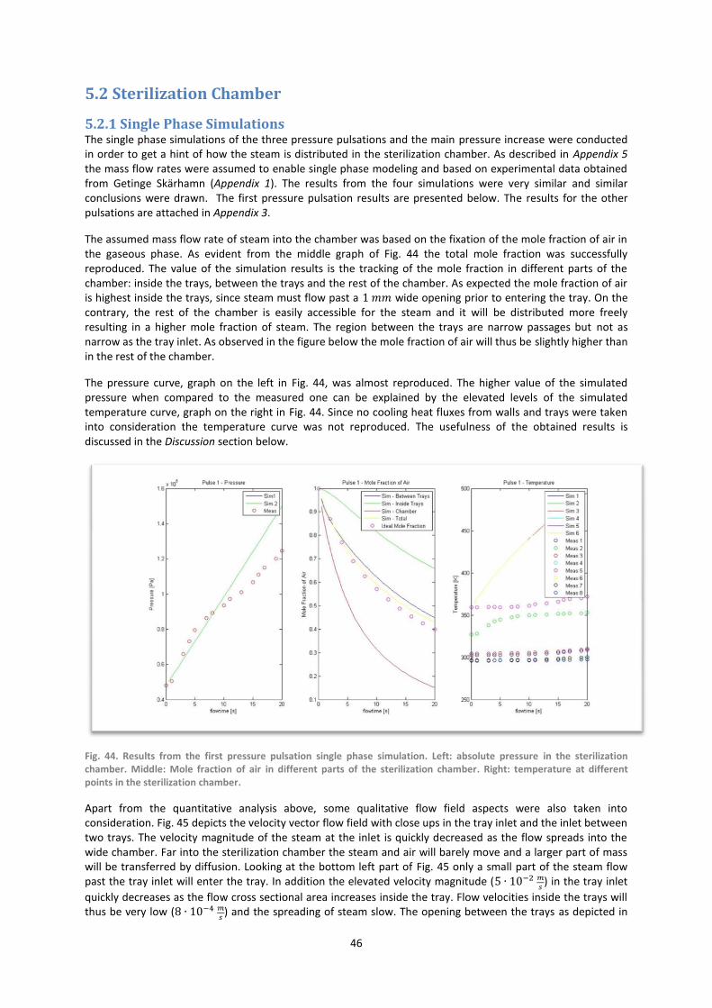
46

5.2 Sterilization Chamber

5.2.1 Single Phase Simulations The single phase simulations of the three pressure pulsations and the main pressure increase were conducted in order to get a hint of how the steam is distributed in the sterilization chamber. As described in Appendix 5 the mass flow rates were assumed to enable single phase modeling and based on experimental data obtained from Getinge Skärhamn (Appendix 1). The results from the four simulations were very similar and similar conclusions were drawn. The first pressure pulsation results are presented below. The results for the other pulsations are attached in Appendix 3.

The assumed mass flow rate of steam into the chamber was based on the fixation of the mole fraction of air in the gaseous phase. As evident from the middle graph of Fig. 44 the total mole fraction was successfully reproduced. The value of the simulation results is the tracking of the mole fraction in different parts of the chamber: inside the trays, between the trays and the rest of the chamber. As expected the mole fraction of air is highest inside the trays, since steam must flow past a wide opening prior to entering the tray. On the contrary, the rest of the chamber is easily accessible for the steam and it will be distributed more freely resulting in a higher mole fraction of steam. The region between the trays are narrow passages but not as narrow as the tray inlet. As observed in the figure below the mole fraction of air will thus be slightly higher than in the rest of the chamber.

The pressure curve, graph on the left in Fig. 44, was almost reproduced. The higher value of the simulated pressure when compared to the measured one can be explained by the elevated levels of the simulated temperature curve, graph on the right in Fig. 44. Since no cooling heat fluxes from walls and trays were taken into consideration the temperature curve was not reproduced. The usefulness of the obtained results is discussed in the Discussion section below.

Fig. 44. Results from the first pressure pulsation single phase simulation. Left: absolute pressure in the sterilization chamber. Middle: Mole fraction of air in different parts of the sterilization chamber. Right: temperature at different points in the sterilization chamber.

Apart from the quantitative analysis above, some qualitative flow field aspects were also taken into consideration. Fig. 45 depicts the velocity vector flow field with close ups in the tray inlet and the inlet between two trays. The velocity magnitude of the steam at the inlet is quickly decreased as the flow spreads into the wide chamber. Far into the sterilization chamber the steam and air will barely move and a larger part of mass will be transferred by diffusion. Looking at the bottom left part of Fig. 45 only a small part of the steam flow past the tray inlet will enter the tray. In addition the elevated velocity magnitude (

) in the tray inlet

quickly decreases as the flow cross sectional area increases inside the tray. Flow velocities inside the trays will thus be very low (

) and the spreading of steam slow. The opening between the trays as depicted in

47

the bottom right part of the figure below is on the other hand large enough for a significant part of the flow to enter. Velocity magnitudes are maintained and possibly even slightly increased as the flow cross sectional area in decreased between the trays. Looking at the top part of the figure however reveals that the incoming flow direction is of great importance to how the distribution of steam between the trays is proceeded.

Fig. 45. Velocity vector figure from the single phase simulation of the first pressure pulsation. Top: Cross-section of the sterilization chamber. Bottom left: close up of the inlet to a tray. Bottom right: close up of the flow in between trays.

The distribution of steam at the end of the first pressure pulsation can be seen in Fig. 46 where the mole fraction of air is depicted in a cross section of the sterilization chamber. It is once more evident that the distribution of steam is slowest inside the trays and fastest in the rest of the chamber. It is interesting to note that the steam seems to ‘push’ the air in front of it. In spite of the low velocities it is likely that some turbulence will be encountered. This would increase species mixing suppressing these ‘pushing’ phenomena. In multiphase simulations this would be even more evident as velocity magnitudes are higher. The placement of the steam inlets and the outlet however seems to be of importance since the main goal is to evacuate as much air as possible. This discussion is extended in the Discussion section.

Fig. 46. Mole fraction of air from the single simulation of the first pressure pulsation.

48

5.2.2 Multiphase Simulations In order to realistically model pressure increase and heating of the sterilization chamber, multiphase simulations including condensation must be conducted. The feasibility of modeling high rates of condensation was investigated with regards to a simplified geometry.

The simulations were conducted using the two meshes presented in the Meshing section above. In both cases, high rates of condensation was successfully computed and monitored by heat and mass balances. The cold solid cools down the fluid part, whereas the steam temperature is lower near the solid-fluid interface. As a result, most condensation took place near the fluid-solid interface as shown in Fig. 47. In the simulation, the rate of condensation was approximately

of the inlet mass flow rate. Therefore, the possibility of modeling the

sufficient condensation rates using FLUENT’s evaporation-condensation model was confirmed.

Fig. 47. The rate of condensation [kg/ (m3·s)]. The left part of the geometry is the solid part, here there is no condensation. The right part of the figure shows the fluid part, the rate of condensation is highest near the solid-fluid interface where the temperature is lower.

Hence, multiphase modeling of the sterilization chamber was considered to be possible to perform but outside the time scope of this thesis work. The same is recommended for future work.

49

6. RECOMMENDATIONS FOR DEVELOPMENT OF A DROPLET BOILING MODEL

The models present in FLUENT are not sufficient for modeling the steam generation in this particular case. To properly describe the real process of nucleate droplet boiling a new model taking the proper physical phenomena into consideration should be developed. Since the problem on hand concerns an evaporating spray there are several events of the transient droplet life that should be treated in the model. Although impossible to resolve all microscopic phenomena, the model should include a physical description of and model droplet-wall impact as well as of the regimes of heat and mass transfer at the wall. In addition, vaporization might alter the structure of the turbulent boundary layers (O’Rourke and Amsden, 1996) whereas special consideration of the turbulence model used must be taken for correct detailed modeling. The following section contains a framework of what such a model could and should include.

6.1 Droplet-Wall Impact and Interaction FLUENT’s DPM model treats the heat and mass transfer to and from dispersed droplets in the bulk sufficiently, whereas it is in vicinity of the wall that the model must be implemented. The onset of the model should be when a droplet impacts the wall. As previously described in Theoretical Framework the transient process of a droplet impacting a wall is quite complex. The droplet impact should thus be modeled, similarly to the wall-film model already implemented in FLUENT. This model includes description of wetting, rebounding and secondary droplet formation at droplet-wall impact as a function of Weber number and surface temperature. Although strictly not a physical description it might be sufficient for the purpose of this model, in addition the number of splashed droplets gives the user a chance to tune the model to the specific system being simulated. If the wall-film impact description is to be reused some features might however need to be added. As evident from the previous description of Droplet-Wall Interactions some more features should be included here such as surface roughness and wettability. A simple but possibly efficient solution could be to include a model coefficient in important equations such as those describing restitution of mass, droplet spreading rate, wall film thickness etc. This could enable the user to tune the model according to experimental data. The criteria of which mode of heat and mass transfer the droplet will enter should be based mainly on the difference between the droplet saturation temperature and the wall temperature. Local values should be used since different regimes can coexist in the system (Ashgriz, 2011). As can be seen in Fig. 10, the onsets of the different regimes are governed by the ONB, CHF and LP points. In order for the model to determine what regime to enter these temperatures must be specified (Schmehl et al., 1999), this should be done with system characteristics and surface properties in mind. As mentioned in Nucleate Boiling it will probably be necessary to experimentally determine important surface properties such as the effect of nucleate site density and cavity shape prior to modeling boiling correctly in specific cases.

6.2 Boiling Regimes As described in the Theoretical Framework section there are four main regimes of heat and interfacial mass transfer during liquid-heated wall interaction: free convection, nucleate boiling, transition boiling and film boiling. Free convection, nucleate boiling and possibly transition boiling are of greatest importance to this model while film boiling should not be included in the model as discussed below.

6.2.1 Evaporation Regime This regime is much simpler to model than nucleate boiling. The interfacial mass transfer occurs at the liquid-vapor surface through relatively slow evaporation, whereas it is not strictly a boiling model. Only liquid is in contact with the wall whereas the heat supplied to the evaporating liquid is transferred through convection and conduction from the wall. Often the impacting droplet is sub-cooled at the given pressure and will require heating in order to reach the saturation temperature. The onset of slow evaporation might however be prior to this since the vapor pressure can exceed the vapor partial pressure in the bulk depending on its composition. This particular regime is well described by FLUENT’s wall-film model and that framework can beneficially be implemented into this model.

6.2.2 Nucleate Boiling Regime Nucleate boiling is as previously described a complex process affected by numerous parameters. It is not possible to reach adequate resolution to model the process in detail. This includes detailed wall surface structure, local effects of bubble growth, bubble departure etc. Much of the RPI model framework can be reused to construct a model of droplet boiling in the nucleate boiling regime. The parameters used as input in

50

the RPI model such as wall temperature, liquid temperature, fluid properties etc. are available from the continuous phase and DPM calculations. As in the RPI model closures will still be needed for the bubble departure diameter, the nucleation site density, and the bubble departure frequency. The closures incorporated into the RPI model could however intrinsically be used in this model as well.

There is however a major difference that needs to be considered. The RPI model was developed for modeling sub-cooled nucleate boiling and the problem on hand differs quite a bit from that, the major difference being the film thickness and coverage of the heated surface. In droplet boiling, the presence of a fully covering liquid film is not guaranteed as opposed to in sub-cooled boiling. In an intense spray situation the film could possibly be considered continuous but most likely it will be of discrete nature. Since the DPM model traces a discrete number of particles the model description of the wall-film in this model should also be discrete.

The process of droplet evaporation at the wall is transient in which the impacting droplet spreads across the surface and then recedes as liquid is consumed in evaporation. The model must thus be able to describe the spreading and receding diameter of droplets, a collection of developed models were summarized by Moreira et al. (2010). Furthermore, the droplet-dry spot boundaries are similar to the micro region as described in Nucleate Boiling. This enhances total evaporation and thus latent heat transfer (Yagov, 2009) which must be included into the model. This could be incorporated through heat and mass transfer correlations as a function of droplet spread diameter. Another issue is the physical description of nucleate boiling as the droplet film thickness decreases due to evaporation. Eventually growing vapor bubbles will extend all the way to the film-vapor bulk interface whereby the vapor of the bubble will enter the vapor bulk instantly. The nucleate boiling description employed in the RPI model will hence become incorrect. An effective solution to this problem could be to relinquish the nucleate boiling description and instead model the dry-out of the droplet separately when the film thickness reaches a critical point. An extensive study on the dry-out process would then have to be conducted. When all liquid has been consumed the model treatment of the droplet and its trajectory is cancelled.

6.2.3 Film and Transition Boiling Regime When the wall superheat exceeds the LP, the droplet is not expected to come in contact with the wall due to the vapor cushion layer formed instantly in between. Droplet film boiling is characterized by very short contact times where heat transfer rates are really low (Bernardin and Mudawar, 1997). Thus, since the most likely droplet-wall interaction is droplet rebound and it is improbable that the droplet impacted by the flow will stick close to the wall when the vapor layer prevents wetting (Chatzikyriakou et al., 2009), film boiling should not be treated by this model. The case of transition boiling is however more complex. In the Theoretical Framework section, transition boiling was described as a blend of nucleate and film boiling. As a consequence of the creation of vapor layers inside the wall film droplet this could even lead to fragmentation of the droplet. This phenomenon must be understood deeper prior to constructing a model. But perhaps a factor of how far from the nucleate boiling regime the model operates can be implemented to account for the departure from the CHF. This factor should then govern heat and mass transfer but also impact droplet spread diameter and wall film thickness. But to implement a realistically correct description of how the transient droplet transition boiling process, an extensive study would have to be conducted to clarify the transition droplet boiling process.

51

7. DISCUSSION This section includes a discussion on the results previously presented. It is divided into two parts, namely steam generator and sterilization chamber.

7.1 Steam Generator Modeling droplet phase transition and droplet boiling in particular is very difficult due to the numerous complex microscopic transport mechanisms involved in the process. As soon as the system characteristics like surface material, surface roughness and wall temperature etc. changes, the character and intensity of the transport mechanisms are significantly influenced. Adding to the complexity of the problem on hand, is the fact that, only evaporation of the fluid generates the flow inside the steam channel whereas single phase simulations cannot predict the flow field. Since this process inside the steam channel has not been observed visually before, the choice of turbulence models, boundary conditions, assumed fluid properties, the RPI model and the droplet boiling model framework are main points that are discussed below.

The choice of turbulence model has already been motivated in the Results section of this thesis work. For continuous phase flow field, the model that has been selected namely SST k-ω turbulence model was found to be appropriate. The numerical investigation conducted in this thesis does not consider the interaction between particles and turbulent flow, both in the free stream and near the walls. Focus was instead laid on the particle-wall interaction since no significance of turbulence on these mechanisms was found in literature studies. The influence of droplet-turbulence interaction can be studied, by enabling a stochastic tracking method, such as the discrete random walk model, to a stable steady state solution. A detailed literature review for a deeper understanding of how boiling, evaporation and turbulence are interrelated on the microscopic scale should be performed starting with the work of O’Rourke and Amsden (1997).

The tested boundary conditions in the part of the steam channel were analyzed in the Results section, in which the choice of the wall-film model is motivated. However, the geometry used in these simulations can be questioned since only a short length of the steam channel is considered. Thus the flow will not have time to fully develop and the largest turbulence length scales are almost of the same order of magnitude as the geometry length. Although there are no inlet turbulence conditions to be specified due to the absence of a continuous phase inlet, the development of turbulence might be incomplete. Out of the four available boundary conditions, the wall-film model was best suited to the problem on hand, despite the fact that it does not contain the physical description of the nucleate boiling regime.

The trap boundary condition could in a more dilute dispersed droplet flow and a longer time step resemble the results of droplet nucleate boiling. The time scale of complete droplet evaporation during nucleate boiling could be of order of magnitude as estimated in hand calculations in Appendix 5. The complete consumption of one droplet is in this case much longer than one time step ( ) as assumed in the instantaneous evaporation of the trap boundary condition. A fundamental difference is in addition the source of enthalpy for evaporation. During nucleate boiling the heat is taken through microscopic phenomena directly from the wall (see Theoretical Framework) whilst in the trap boundary condition all heat is taken from the fluid near the wall (ANSYS Inc., 2011). This provides problems which were evident in Fig. 37 where a high droplet-wall impact rate will introduce unnatural local cooling.

The source of enthalpy for evaporation in the wall-film model is also the cell closest to the wall. Consequently unrealistic cooling near the wall is a possible issue when using the wall-film model as well. The evaporation of a droplet is however much slower than when using the trap model, whereas the local enthalpy sinks will not be as large. The wall-film model has another problem making results harder to analyze, the presentation of wall heat flux. The heat transfer to the wall-film is subtracted from the heat flux to the continuous phase whereas the total surface heat flux is impossible to determine. Wall heat flux must consequently be determined indirectly from a particle and continuous phase heat balance.

The simulation of the full steam channel using real fluid properties did not yield the desired results. Not surprisingly the rate of heat and mass transfer to the DPM particles was not sufficient since the correct physical description of the particle-wall interaction was not incorporated into the wall-film model. To reproduce the rate of evaporation in nucleate boiling assumed fluid properties were used. One could argue that there is a similarity between defining a constant ‘effective thermal conductivity’ just like the early turbulence models were based on the setting of a constant effective viscosity. Of course this way of modeling nucleate boiling is

52

not physically correct but it can yield realistic macroscopic results. Due to the absence of sufficient experimental data to validate the assumed fluid property simulation, it is hard to draw concrete conclusions. Apart from overestimating heat transfer to the fluids slightly the results seem relatively realistic. Future work should however be based on conducting appropriate process measurements on different points inside the steam channel prior to modeling. This would enable a macroscopic tuning to system characteristics. The obtained simulation setup when using assumed fluid properties can then be used to analyze trends but not details of the steam channel design.

Firstly, focus in this thesis was on obtaining a stable steady state simulation. A constant wall temperature of was applied in order to reach a steady state solution. In a transient solution this would however be an incorrectly defined temperature boundary condition since it would allow a continuous high rate of vaporization. In reality the wall must be cooled down when droplets boil on it. In future transient simulations the full steam generator should thus be modeled including the whole solid aluminum part. The temperature fluctuations inside the aluminum solid could then be investigated while simultaneously obtaining the correct steam channel surface temperatures.

The RPI model within the Eularian-Eularian multiphase model was considered for use. The model is developed in the context of sub-cooled flow boiling and not for droplet boiling. Some trembling attempts were made to implement the RPI model. The results are however not worth mentioning in this thesis. After personal communication with RPI model developer Professor Michael Podowski on September 19

th, 2012 the plans of

applying the existing model to the problem on hand were discouraged and abandoned. The reuse of some of the RPI model’s theoretical formulation was however discussed in the Droplet Boiling Model Framework.

The droplet boiling model framework presented in the Results section is a rough description of a potential droplet boiling model. Such a model would incorporate droplet-wall impact, droplet boiling and dry-out. The theoretical parts are based on reports in literature and the RPI model as presented in the FLUENT manual (ANSYS Inc., 2011). The development of such a model would be appropriate for solving problems of spray steam generators but also spray cooling, steel quenching and possibly internal chamber automotive problems. The development of such an extensive model can however not be incorporated in a master’s thesis timeframe. It would also require a deeper knowledge understanding of the important transport phenomena than that possessed of a master’s student.

7.2 Sterilization Chamber The sterilizing process inside the sterilization chamber does also include phase transition, namely condensation. The problem on hand is quite difficult as approximately 80 % of the mass flow rate at the inlet is expected to condense on trays and chamber walls. The validity of the single phase simulations can therefore be questioned and is discussed in the paragraph below. The use of the evaporation-condensation model within the mixture multiphase model is subsequently discussed in the next paragraph.

The assumption of single phase flow in the steam channel is not valid for realistic modeling of the sterilization process. The inlet mass flow rate was assumed so as to reproduce the mole fraction of air in the gaseous phase after the pressure pulsation. Hence, the condensation of steam was not considered. The real mass flow rate will be several times higher than the assumed one. Since condensed steam is evaporated again when the pressure decreases because of the vacuum system, the air will be diluted with even more steam than anticipated in the single phase simulations. The simulations are therefore quantitatively not useful. However, the same are important to get a basic understanding of distribution of steam in the sterilization chamber. For example the relative distribution of the air mole fraction in different parts of the chamber can provide information about where inlets and outlets can be placed.

There are other parameters to be considered since increase in mass flow rate leads to higher velocity magnitudes and the condensation at walls. This will in turn disrupt the single phase flow pattern. When steam condenses the local pressure will decrease inducing a flow towards that region. In colder regions of the chamber, inside the trays in particular, more condensation is expected at the walls. This will generate local low pressure regions that lead the steam, through the narrow openings, into the trays. The effects of such condensation pressure decreases may reduce the validity of the single phase simulations.

Also, higher mass flow rates and increased velocities lead to the fact that the flow becomes turbulent. Both macro and micro mixing of steam and air will thus be enhanced. As a result, more homogenous contours of the

53

steam and air molar fractions are obtained when compared to the single phase simulations. The results obtained from single phase simulations should be used with caution. In order to realistically analyze the system, a suitable multiphase condensation model needs to be implemented.

In general, the numerical simulations to model phase change are difficult, especially when rates of phase change are high compared to the total mass flow rate in the system. Furthermore, large gradients in pressure and temperature will occur and therefore for complex geometries it is difficult to obtain numerical stability. However simulations conducted for simple geometries showed that, modeling of very high rates of condensation is possible. Since, in this thesis, to obtain a better understanding of nucleate boiling and modeling of the steam generator was given the importance, detailed investigations on multiphase modeling of the sterilization chamber is recommended in future work.

54

8. CONCLUSION Firstly, the conclusions regarding the steam generator and sterilization chamber are presented. Secondly, objectives, results and future work are summarized.

8.1 Steam Generator Water droplets are expected to enter the nucleate boiling regime as they impact the wall in the steam generator when the surface and wall properties are considered. Theoretical descriptions of nucleate boiling and droplet-wall impact are identified and presented. The inherent complexity of boiling transport phenomena are compared to the theoretical basis of existing discrete particle boundary condition models in FLUENT, none of which can be used in order to realistically predict droplet nucleate boiling. The RPI model was examined but not considered for use in the thesis after personal communication with model co-developer Professor Michael Podowski on September 19

th, 2012. Instead the fluid properties, thermal conductivity and binary diffusivity

were tuned to obtain globally realistic results when FLUENT’s wall-film model was applied.

Although not completely validated, due to lack of experimental data, this procedure is a possible tool to analyze the heat and mass transfer processes inside the steam generator. However, the level of detail with respect to transport phenomena in the steam generator is limited due to the assumed fluid properties. Furthermore, a droplet boiling model framework has been presented specifying the important aspects that needs to be considered in the future development of a droplet boiling model within the discrete particle method. In short, continued simulation using the assumed fluid properties procedure and development of a droplet boiling model are two possible topics of future work.

8.2 Sterilization Chamber Quantitative results from modeling of the sterilization chamber are obtained for single phase simulations only. The results can be used for predicting general trends of steam distribution in the chamber. The validity of the single phase simulations can however be questioned since an assumed inlet mass flow rate differing substantially from the measured one was used. The placement of inlets and outlet are aspects worth investigating further. The mixture multiphase model was then used to model condensation in the chamber. In spite of conducting several investigations the solution using full scale geometries diverged. Extremely simplified simulations did however confirm that high rates of condensation are possible to model. Further simulations were not carried out because of the time limit of the thesis. Instead this is recommended as a topic of future work.

8.3 General Summary The following are the points that summarize the thesis work:

a. The objectives that were identified for thesis work are mostly fulfilled and the research questions have been extensively treated.

b. The phenomena of phase change in general and nucleate boiling in particular are studied extensively and presented in the thesis.

c. The droplet-wall interaction process has been studied. d. The process of steam generation in the steam generator has thus been investigated thoroughly and

understood. e. The modeling of droplet nucleate boiling using existing FLUENT models is limited to obtain

macroscopically correct results by assuming some transport properties of the involved phases. f. For detailed analysis a new droplet boiling model has to be developed and implemented. g. The general trends of how steam inside the sterilization chamber is distributed have been

investigated. h. The feasibility of modeling high rates of condensation was successfully computed with regards to

simplified simulations. i. The fundamental problems of modeling high rates of condensation have been identified and partly

solved.

8.4 Future Work The following points are recommended for future work based on this thesis.

55

a. Further CFD analysis of the steam generator using the assumed fluid properties. b. Extending the steam generator geometry to also include the solid aluminum parts in transient

simulations. c. Research and development work on the proposed droplet boiling model in order to enable a realistic

and detailed analysis. d. Modeling distribution of steam including condensation in the sterilization chamber. e. Parameter studies for both the steam generator and sterilization chamber should be performed taking

into consideration the design aspects of Getinge Skärhamn’s to improve the performance and decreased process time, volume and weight of the autoclave.

56

9. REFERENCES

Andersson, B., Andersson, R., Håkansson, L., Mortensen, M., Sudiyo, R. and van Wachem, B. (2012) Computational Fluid Dynamics for Engineers. Cambridge: Cambridge University Press.

ANSYS Inc. (2011) FLUENT Documentation, ANSYS 14.0. Software guide bundled with ANSYS FLUENT v.14.0 (Accessed 2012-06-25).

Ashgriz, N. (2011) Handbook of Atomization and Sprays. [Electronic]. New York: Springer Science+Business Media.

Bansal, N.K. and Shail. (1999) Characteristic parameters of a hypocaust construction. Building and Environment, vol. 34, no. 3, pp. 305-318.

Baumeister, K.J., Henry, R.E. and Simon, F.F. (1970) Role of surface in the measurement of the Leidenfrost temperature. Glenn Research Center: NASA. (NASA report: NASA-TM-X-52866, E-5828).

Bernardin, J.D., Mudawar, I. (1997) Film boiling heat transfer of droplet streams and sprays. International Journal of Heat and Mass Transfer, vol. 40, no. 11, pp. 2579-2593.

Bernardin, J.D., Stebbins, C.J. and Mudawar, I. (1997) Effects of surface roughness on water droplet impact history and heat transfer regimes. International Journal of Heat and Mass Transfer, vol. 40, no. 1, pp. 73-88.

Bernardin, J.D., Stebbins, C.J. and Mudawar, I. (1997) Mapping of impact and heat transfer regimes of water drops impinging on a polished surface. International Journal of Heat and Mass Transfer, vol. 40, no. 2, pp. 247-267.

Biance, A.L., Clanet, C. and Quere, D. (2003) Leidenfrost drops. Physics of Fluids, vol. 15, no. 6, pp. 1632-1637.

Capitao Patrao, A. et al. (2010) Ångalstrare för en autoklav. Göteborg: Chalmers University of Technology. (Bachelor’s Thesis at Institution of Applied Mechanics.)

Chatzikyriakou, D., Walker, S.P., Hewitt, G.F., Narayanan, C. and Lakehal, D. (2009) Comparison of measured and modeled droplet-hot wall interactions. Applied Thermal Engineering, vol. 29, pp. 1398-1405.

Das, A.K., Das, P.K. and Saha, P. (2006) Nucleate boiling of water from plain and structured surfaces. Experimental Thermal and Fluid Science, vol. 31, pp. 967-977.

Del Valle, V.H. and Kenning, D.B.R. (1985) Subcooled flow boiling at high heat flux. International Journal of Heat and Mass Transfer, vol. 28, no. 10, pp. 1907–1920.

Dhir , V.K. and Liaw, S.P. (1989) Framework for a Unified Model for Nucleate and Transition Pool Boiling. Journal of Heat Transfer, vol. 111, pp. 739-746.

Elliot, J.R. and Lira, C.T. (2006) Introductory Chemical Engineering Thermodynamics. Upper Saddle River: Prentice Hall.

Genske, P. and Stephan, K. (2006) Numerical simulation of heat transfer during growth of single vapor bubbles in nucleate boiling. International Journal of Thermal Sciences, vol. 45, pp. 299-309.

Getinge Skärhamn AB (2012), Products/Getinge Quadro. http://www.getinge.com/healthcare/products/sterilization/steam-sterilizers/getinge-quadro/ (Accessed 2012-11-02).

Jo, H., Ahn, H.S., Kang, S. and Kim, M.H. (2011) A study of nucleate boiling heat transfer on hydrophilic, hydrophobic and heterogeneous wetting surfaces. International Journal of Heat and Mass Transfer, vol. 54, pp. 5643-5652.

57

Kalantari, D. and Tropea, C. (2007) Phase Doppler measurements of spray impact onto rigid walls. Experiments in Fluids, vol. 43, no. 2, pp. 285-296.

Krause, F., Schuttenberg, S. and Fritsching, U. (2010) Modelling and simulation of flow boiling heat transfer. International Journal of Numerical Methods for Heat & Fluid Flow, vol. 20, iss. 3, pp. 312-331.

Krepper, E., Koncar, B. and Egorov, Y. (2006) CFD modeling of subcooled boiling – Concept, validation and application to fuel assembly design. Nuclear Engineering and Design, vol. 237, pp. 716-731.

Kurul, N. and Podowski, M.Z. (1996) On the modeling of multidimensional effects in boiling channels. In Proceedings of the 27th National Heat Transfer Conference; 1991, Minneapolis.

Luke, A. (2010) Interactions between bubble formation and heating surface in nucleate boiling. Experimental Thermal and Fluid Science, vol. 35, pp. 753-761.

ME Department (2012), Multiphase & Cardiovascular Flow Lab. http://fluids.me.washington.edu/droplet-impact.html (Accessed 2012-10-01).

Mei, R. (1995) Vapor bubble growth in heterogeneous boiling – I. Formulation. International Journal of Heat and Mass Transfer, vol. 38, no. 5, pp. 909-919.

Mei, R. (1995) Vapor bubble growth in heterogeneous boiling – II. Growth rate and thermal fields. International Journal of Heat and Mass Transfer, vol. 38, no. 5, pp. 921-934.

Moreira, A.L.N., Moita, A.S. and Panao, M.R. (2010) Advances and challenges in explaining fuel spray impingement: How much of single droplet impact research is useful?. Progress in Energy and Combustion Science, vol. 36, pp. 554-580.

Mörstedt, S. and Hellsten, G. (1999) Data och diagram: Energi- och kemitekniska tabeller. Seventh edition. Stockholm: Liber.

Mosdorf, R. and Shoji, M. (2004) Chaos in nucleate boiling – nonlinear analysis and modeling. International Journal of Heat and Mass Transfer, vol. 47, pp. 1515-1524.

Mudawar, I. and Valentine, W.S. (1989) Determination of the Local Quench Curve for Spray-Cooled Metallic Surfaces. Journal of Heat Treating, vol. 7, no. 2, pp. 107-121.

Narumanchi, S., Troshko, A., Bharatan, D. and Hassani, V. (2008) Numerical simulations of nucleate boiling impinging jets: Applications in power electronics cooling. International Journal of Heat and Mass Transfer, vol. 51, pp. 1-12.

O’Rourke, P.J. and Amsden, A.A. (1996) A Particle Numerical Model for Wall Film Dynamics in Port-Injected Engines. SAE Fuels and Lubricants Meeting; October 14-17, 1996, San Antonio.

Pan, K.L. and Law, C.K. (2007) Dynamics of droplet-film collision. Journal of Fluid Mechanics, vol. 587, pp. 1-22.

Petrovic, S., Robinson, T. and Judd, R.L. (2004) Marangoni heat transfer in subcooled nucleate pool boiling. International Journal of Heat and Mass Transfer, vol. 47, pp. 5115-5128.

Phan, H.T., Caney, N., Marty, P., Colasson, S. and Gavillet, J. (2009) How does surface wettability influence nucleate boiling?. C. R. Mecanique, vol. 337, pp. 251-259.

Podowski, M.Z. (2008) Multidimensional modeling of two-phase flow and heat transfer. International Journal of Numerical Methods for Heat & Fluid Flow, vol. 18, iss. 3, pp. 491-513.

Rioboo, R., Marengo, M. and Tropea, C. (2002) Time evolution of liquid drop impact onto solid, dry surfaces. Experiments in Fluids, vol. 33, pp. 112-124.

http://fluids.me.washington.edu/droplet-impact.html

http://fluids.me.washington.edu/droplet-impact.html

58

Schmehl , R., Rosskamp, H., Willmann, M. and Wittig, S. (1999) CFD analysis of spray propagation and evaporation including wall film formation and spray/film interactions. International Journal of Heat and Fluid Flow, vol. 20, pp. 520-529.

Stephan, P. and Fuchs, T. (2009) Local heat flow and temperature fluctuations in wall and fluid in nucleate boiling systems. Heat Mass Transfer, vol. 45, pp. 919-928.

Stephan, P. and Kern, J. (2004) Evaluation of heat and mass transfer phenomena in nucleate boiling. International Journal of Heat and Fluid Flow, vol. 25, pp. 140-148.

Tennekes, H. and Lumley, J.L. (1972) A first course in turbulence. Cambridge: MIT Press. Cited in B. Andersson, Computational Fluid Dynamics for Engineers. Eight edition. Gothenburg: Cambridge University Press. (2012) pp. 76-80.

Tong, L.S. (1971) Heat-transfer mechanisms in nucleate and film boiling. Nuclear Engineering and Design, vol. 21, pp. 1-25.

Vårdhandboken (2011), Medicintekniska produkter, sterilisering: Inaktivering med torr mättad ånga (ångautoklav). http://www.vardhandboken.se/Texter/Medicintekniska-produkter-sterilisering/Metoder-och-kontroller/ (Accessed 2012-06-21).

Welty, J.R., Wicks, C.E., Wilson, R.E. and Rorrer, G.L. (2008) Fundamentals of Momentum, Heat, and Mass Transfer. Fifth edition. New York: Wiley.

Wolfram Alpha (2012), WolframAlpha computational knowledge engine. http://www.wolframalpha.com/ (Accessed 2012-07-02).

Yagov, V.V. (2009) Nucleate boiling heat transfer: possibilities and limitations of theoretical analysis. Heat Mass Transfer, vol. 45, pp. 881-892.

Zeng, L.Z., Klausner, J.F. and Mei, R. (1993) A unified model for the prediction of bubble detachment diameters in boiling systems – I. Pool boiling. International Journal of Heat and Mass Transfer, vol. 36, no. 9, pp. 2261-2270.

Zeng, L.Z., Klausner, J.F., Bernhard, D.M. and Mei, R. (1993) A unified model for the prediction of bubble detachment diameters in boiling systems – II. Flow boiling. International Journal of Heat and Mass Transfer, vol. 36, no. 9, pp. 2271-2279.

http://www.wolframalpha.com/

59

APPENDIX 1: Sterilization Process Measurements Pressure and temperature measurements of a typical Quadro series sterilization process.

Fig. 48. The measured absolute pressure of a typical sterilization process. Values have been classified.

60

Fig. 49. The measured temperature of a typical sterilization process at 8 points in the sterilization chamber. Points 1, 3-4 and 6-8 are placed on trays while points 2 and 5 are placed near the chamber outer walls. Values have been classified.

61

APPENDIX 2: User Defined Functions UDF for specifying mass flow rate as a function of time:

UDF for specifying inlet temperature to saturation temperature as a function of operating pressure:

62

APPENDIX 3: Sterilization Chamber Single Phase Results

Fig. 50. Results from the second pressure pulsation single phase simulation. Left: absolute pressure in the sterilization chamber. Middle: Mole fraction of air in different parts of the sterilization chamber. Right: temperature at different points in the sterilization chamber.

Fig. 51. Results from the third pressure pulsation single phase simulation. Left: absolute pressure in the sterilization chamber. Middle: Mole fraction of air in different parts of the sterilization chamber. Right: temperature at different points in the sterilization chamber.

63

APPENDIX 4: Basic Concepts of Fluid Mechanics

Laminar and Turbulent Flow

Flow can be characterized by laminar and turbulent flow conditions. When viscous forces are much larger than inertial forces the flow is said to be stable and laminar. When inertial forces are comparable and larger than viscous forces the flow becomes unstable and turbulent (Welty et al., 2008; Andersson et al., 2012). The Reynolds number is used as an indicator of the transition between laminar and turbulent flow where low Reynolds numbers imply laminar flow and vice versa. Laminar flow is well-ordered regular flow and turbulence is a condition of flow where quantities show random variation in time and space but where statistical average values can be obtained (Andersson et al., 2012).

Tennekes and Lumley (1972) have identified and listed seven characteristic features of turbulent flows:

1. Turbulence is irregular and consists of a range of coexisting length, velocity and time scales. 2. Turbulence is diffusive allowing fast mixing of species, momentum and energy through turbulent

diffusive transport. 3. Turbulence arises from instability at large Reynolds numbers. 4. Turbulence is three-dimensional and cannot occur in fewer dimensions. 5. Turbulent kinetic energy is dissipated from larger to smaller turbulent scales and eventually dissipated

into heat by viscous forces. 6. The smallest scales of turbulence are much larger than the molecular scale whereas turbulent flow is a

continuum phenomenon. 7. Turbulence is a feature of the flow and not of the fluid.

Compressible and Incompressible Flow

In incompressible flow the density is constant. When the velocity of the gases is more than one third the velocity of sound, the flows are termed compressible (Welty et al., 2008; Andersson et al., 2012). Pressure waves are spread with the speed of sound and the variation of density due to these waves can thus be neglected if the gas velocity is low in comparison.

Boundary Layers

Flow parallel to a surface induces the formation of a boundary layer. The velocity at the surface is assumed to be zero and is commonly referred to as the no slip condition. This produces a velocity profile normal to the surface as seen in Fig. 52. Likewise if there is a temperature difference between the surface and the bulk there will be a similar temperature profile normal to the surface (Welty et al., 2008).

Fig. 52. The velocity boundary layer near the wall. Velocity increases parabolically as a function of distance from the wall.

Boundary layers are of great importance when considering turbulent flow conditions. The low velocity near the wall results leads to the formation of three distinguishable sub-layers: the viscous, buffer and fully turbulent sub-layers (Fig. 53). The viscous sub-layer is characterized by laminar flow conditions where molecular viscosity governs momentum transfer. The buffer sub-layer is a transition region of both laminar and turbulent flow where molecular and turbulent viscosities are of equal importance. The fully turbulent sub-layer is characterized by turbulent flow conditions where turbulent viscosity governs momentum transfer (Andersson et al., 2012). Consideration of the sub-layers is of great importance in CFD turbulence modeling.

64

Fig. 53. The turbulent boundary layer near the wall consisting of a viscous, a buffer and a fully turbulent sub-layer (Bansal and Shail, 1999).

65

APPENDIX 5: Hand Calculations Before simulations were performed some general hand calculations was conducted. The purpose of the same is to investigate and understand important system characteristics. The same is done, also, to obtain crude approximations to check simulation validity. The calculations are divided into the two sections namely steam generator and sterilization chamber. Known process data is specified in Table 4.

Table 4. Known sterilization process data used for hand calculations. Values have been classified.

Variable Denotation Value

Volumetric Flow Rate -

Volumetric Flow Rate -

Water Temperature Inlet -

Initial Wall Temperature of Steam Channel -

Steam Channel Inlet Cross-sectional Area -

Steam Channel Cross-sectional Area -

Steam Channel Outlet Cross-sectional Area -

Steam Channel Surface Area -

Steam Channel Diameter -

Steam Channel Length -

Steam Channel Volume -

Sterilization Chamber Inlet Cross-sectional Area -

Sterilization Chamber Inlet Characteristic Length -

Sterilization Chamber Volume -

Sterilization Chamber Walls Steel Mass -

Sterilization Chamber Tray Aluminum Mass -

Sterilization Chamber Load Steel Mass -

Median Droplet Diameter -

Fluid and solid material data are shown in Table 5 below. Specific conditions at which the material data is valid is also given in the same.

Table 5. Fluid and solid material data relevant for hand calculations.

Variable Denotation Value Specific Condition

Molar Mass Water

(Mörstedt and Hellsten, 2008)

Molar Mass Air


Specific Heat Capacity Water


Specific Heat Capacity Aluminum


Specific Heat Capacity Steel


Heat of Vaporization Water


Density Water


Density Steam

Sat. Steam at (Mörstedt and Hellsten, 2008)



Density Aluminum


Stefan-Boltzmann Constant

(Welty et al., 2008))

Dynamic Viscosity Steam and (Wolfram Alpha, 2012)

Surface Tension Water

and (Wolfram Alpha, 2012)

Mean Free Path and

Thermal Conductivity Steam

(Wolfram Alpha, 2012)

66

Steam Generator

Momentum Calculations

First of all, some basic calculations concerning the steam channel velocity field were conducted. The mass flow

rate ( ) was determined from the volumetric flow rate of liquid water ( ) provided by Getinge

Skärhamn as in Eq. (28).

(28)

All injected water was assumed to evaporate in the steam channel and the volumetric flow rate of steam was calculated under three different pressure conditions in Eqs. (29) to (31).

(29)

(30)

(31)

Using the steam volumetric flow rate it was possible to calculate the expected velocities through the steam channel at the given pressures, Eqs. (32) to (34).

(32)

(33)

(34)

The droplet velocity in the inlet was calculated through the volumetric flow rate of water and the injector inlet cross-sectional area, Eq. (35).

(35)

Heat Calculations

To obtain an initial understanding of the heat transfer in the system, some general heat calculations were executed. The total power required to evaporate the water into steam was calculated in Eq. (36).

(36)

The average heat flux from the walls of the steam channel was approximated in Eq. (37).

(37)

The contribution of radiant heat transfer was approximated in order to conclude its insignificance in simulations as shown in Eq. (38). The steam channel walls were assumed to be perfect radiators in order to calculate the maximum possible radiation heat transfer so that its significance was not underestimated.

(38)

Compared to the total effect needed, radiant heat transfer was negligible. The dominating heat transfer mechanism to the fluid occurs through convection and boiling at walls.

67

Dimensionless Numbers

Some dimensionless parameters have been determined in order to characterize the system. Firstly, the Reynolds number in the steam channel was determined as in Eqs. (39) to (41). For the three important pressure conditions the same is calculated when all liquid water evaporates to steam.

(39)

(40)

(41)

The transition from laminar to turbulent flow normally occurs at for internal pipe flow, the flow in the steam channel is therefore fully developed turbulent flow. To understand droplet behavior and to identify and select a multiphase model, the Weber number at atmospheric pressure has been determined in Eq. (42). The relatively high Weber number indicated that particles are likely to impact wall with fairly high momentum and splash in droplet-wall interaction.

(42)

The Knudsen number was determined, in Eq. (43), to investigate whether there is a significant influence of particle collisions in numerical simulations. The Knudsen number was determined at as particle collisions are more likely to be more influential at lower pressures. The low value of the calculated Knudsen number indicates that the rarefaction effect is not significant and can be neglected.

(43)

To estimate the momentum and thermal interaction between the droplets and fluid phase, the momentum and thermal Stokes numbers were determined in Eqs. (44) to (49). The characteristic time constants used in calculations are described under the Particle Response Time section below. High Stokes numbers ( ) imply that the droplet will not be affected by the flow. The relatively high Stokes numbers determined in Eqs. (44) to (49) below, indicates that momentum and heat transfer of the droplets does not completely be governed by the flow conditions. In addition the high momentum Stokes numbers imply that the droplets will most likely hit the wall of the sterilization chamber. The droplet-wall interaction treatment will thus be important in modeling the system.

(44)

(45)

(46)

(47)

(48)

(49)

Turbulence Scales

To get a basic understanding of turbulence properties in the steam generator some turbulence quantities were estimated. Firstly the turbulence intensity ( ) and length scale ( ) were approximated according to Eqs. (50) and (51).

(50)

(51)

Using these calculated quantities, the channel mean flow and the coefficient ( ); the turbulence

kinetic energy and turbulence dissipation rate were determined in Eqs. (52) and (53).

68

(52)

(53)

Using this and the molecular viscosity of steam the length, time and velocity scales of the largest turbulence eddies were determined in Eqs. (54) to (56). The same scales of the smallest eddies were determined in Eqs. (57) to (59).

(54)

(55)

(56)

(57)

(58)

(59)

The estimated length scale of the largest eddies is , quite large compared to system dimensions. Turbulence is thus not expected to be isotropic, hence the Boussinesq approximation can be questioned. Applying a large-eddy simulation turbulence model is a possible solution but the scales determined in Eqs. (54) to (56) must then be properly resolved. The computational cost for this is not possible to fit inside the scope of this thesis work therefore a two-equation model will be considered sufficient.

(60)

The turbulence boundary conditions will thus last into the geometry during single phase turbulence modeling according to Eq. (60).

Particle Response Times

Momentum and thermal particle response times were calculated to obtain an understanding of how far into the system the particle boundary conditions lasted. Firstly, the flow response times ( ) were calculated in Eqs. (61) to (63).

(61)

(62)

(63)

The droplet velocity response time is fairly constant in the pressure range and was calculated using Eq. (64) (Crowe, 2006). This is a measure of the time it takes for the droplet to react to a step change in velocity.

(64)

During this time the particle will travel the distance Eq. (65). Thus if a droplet was to be injected straight through the channel it would not have time to react completely to the step change in velocity. The droplets are however injected with an angle aimed at the walls whereas it will lose some of its kinetic energy.

(65)

Similarly, the droplet thermal response time is relatively insensitive to pressure and was calculated according to Eq. (66) (Crowe, 2006). This is a measure of the time it takes for the droplet to react to a step change in temperature.

(66)

69

During this time the particle will travel the distance Eq. (67).

(67)

Coupling Parameters

To determine whether coupling effects are important, numerical simulations for the mass, momentum and thermal coupling parameters ( , , ) were calculated. The mass coupling was calculated by Eq. (68). This evidently implies a strong two-way coupling between the phases which was expected since evaporation is the only source of steam in the steam channel.

(68)

To determine the momentum and thermal coupling parameters, the apparent densities of the continuous phase (steam) and dispersed phase (water droplets) are to be estimated. From initial simulations, the accumulated mass of droplets in the system at steady state was which corresponds to a liquid volume of . The apparent density of the dispersed phase was thus calculated through Eq. (69). Since the volume fraction of the continuous phase is high it was assumed that .

(69)

The momentum coupling parameter was determined at three pressure levels in Eqs. (70) to (72).

(70)

(71)

(72)

Similarly, the thermal coupling parameter was determined at the same pressure levels in Eqs. (73) to (75).

(73)

(74)

(75)

The momentum and thermal couplings are evidently weaker than the mass coupling. The coupling parameter does not however consider droplet-wall interaction but mainly the effects of the particle dispersion. Similarly to the reasoning of the determined Stokes numbers above, it is evident that droplet-wall interaction will be of uttermost importance during modeling.

DPM Time Steps

In order to determine appropriate particle time step size during simulations, some investigative estimations were made. One aspect that needs to be resolved with sufficiently small time steps when using the wall-film model is the process of evaporating one droplet. The time to evaporate one droplet was estimated using some crude approximations. The average droplet’s cross sectional area was assumed to be the spreading diameter of an impinged droplet. The heat flux from the wall was assumed to be the average calculated in Eq. (37) above. Using these assumptions the time of evaporation was estimated from Eqs. (76) to (81). The time steps should thus be significantly shorter than to resolve droplet evaporation in the wall-film.

(76)

(77)

(78)

(79)

70

(80)

(81)

Another aspect to consider is that a DPM particle should not pass a computational cell during one time step, thus the particle velocity was related to the approximate cell size whereas the critical time step size was determined. To obtain a rough approximation of the element size they were assumed to be quadratic boxes. The length of one side was estimated in Eq. (82).

(82)

(83)

With the initial droplet velocity previously stated, the particle would travel through the cell in {Eq. (83)}. The appropriate time step should therefore be smaller and preferably with magnitude . This is however the worst case scenario and droplets quickly experience decreased velocity as they impact the wall. When a particle travels past multiple cells in one time step FLUENT applies an algorithm automatically decreasing the time step to update particle sources in each cell. Since previous calculations imply that particle sources before wall-impact are limited in influence and in order to decrease computational times it is thus assumed viable with a time step of .

Sterilization Chamber

Mass Calculations

Assumed Filling and Emptying of Sterilization Chamber

Getinge Skärhamn could not guarantee the water mass flow rate measurement to be accurate and therefore the measurements were conducted as shown in Table 4 above. Calculations with respect to assumed mass flow rate were executed prior to conducting single phase simulations. The same was executed, for four stages of steam supply in to the sterilization chamber (see Fig. 4), namely three pressure pulsations and the main pressure increase, prior to the sterilization stage. Table 6 below, provides the time and important parameter values of the system at the above mentioned stages.

Table 6. Initial and final points of the pressure pulsations during the sterilization process. The state of the system is given at each time.

Stage Time Temperature Pressure Molar Density

Pulse 1 00:53

01:21

Pulse 2 02:49

03:44

Pulse 3 06:55

07:41

Main Pressure Increase 11:15

12:27

16:08

The volume is known, whereas the mole fraction of each species in the chamber can be approximated. If one assumes perfect mixing at all times one can determine the ideal remainder of air at the sterilization stage through the algorithm in Eqs. (84)-(89). The mole fraction of air ( ) is equal to one prior to the first pressure pulse.

71

(84)

(85)

Pressure increased through addition of steam.

(86)

(87)

Pressure decreased as outlet valve is opened.

(88)

(89)

The next pulse is then started whereas the procedure is repeated. Using the algorithm above the ideal amount of air present after each pulsation was determined and presented in Table 7. Evidently, the amount of air decreases quickly and linearly with the amount of added steam.

Table 7. The ideal amount of air present after each pressure pulsation.

Stage Mole Fraction of Air Mass of Air

Pulse 1

Pulse 2

Pulse 3

Main Pressure Increase

Assumed Mass Flow Rate for Single Phase Simulations

Prior to modeling the pulsations in single phase, the assumed mass flow rate needed to be approximated for the case of no condensation. This was done using the volume of the chamber, the moles of gas present in the chamber at the times given in Table 6 could be determined from the ideal gas law as in Eq. (90). The assumed mass flow rate of steam into the chamber can therefore be determined from Eq. (91) and the assumed mass flow rates used in single phase simulations are summarized in Table 8 below.

(90)

(91)

Table 8. The determined assumed mass flow rates for single phase simulations of the sterilization chamber.

Stage Assumed Mass Flow Rate

Pulse 1

Pulse 2

Pulse 3


Rate of Condensation

The actual rate of condensation under the duration of one pulsation could be determined through using the measured mass flow rate and setting up a mass balance as in Eq. (92). Masses and are in the gaseous phase prior to and after the pulsation. The rates of condensation are thus assumed constant during the pulsation and are summarized in Table 9.

(92)

Table 9. The average rate of condensation during pressure pulsations.

Stage Rate of Condensation

Pulse 1

72

Pulse 2

Pulse 3


In the scope of this investigation, only single phase simulations were carried out with respect to distribution of steam. However, since the rate of condensation is very large compared to the inlet mass flow rate during the sterilization process, multiphase simulations are recommended in order to predict the high condensation rate that is bound to occur.

Inlet Velocity

During simulations merely the mass flow rate was specified as inlet condition. To understand system characteristics and also to be able to determine the inlet Reynolds number, the inlet velocities were approximated. Given the measured mass flow rate, the inlet velocities at in the sterilization chamber were calculated using Eqs. (93) to (95).

(93)

(94)

(95)

Heat Calculations

For understanding global heat transfer in the system the magnitude of heat transfers in different parts of the sterilization chamber were determined for the main pressure increase stage applying Eqs. (96) to (99).

(96)

(97)

(98)

(99)

The sterilization chamber walls are also partly covered by an electrical heating mat generating .

The walls, trays and condensed water is heated to the sterilization temperature ( ) resulting in ,

and respectively. Heat from the electrical heating mat is much lesser than the latent heat released

during the condensation process. Most of the heat provided during the sterilization process is due to release of the latent heat from condensation and therefore needs to be further investigated.

Dimensionless Numbers

The Reynolds number was determined in order investigate the presence of turbulence. The characteristic length of the inlet was assumed to be yielding the inlet Reynolds number, Eqs. (100) to (102).

(100)

(101)

(102)

The above values of the Reynolds number clearly indicate that the flow is turbulent in the system. In case of the assumed mass flow rate for single phase simulations (see Table 8), the Reynolds number is expected to be approximately 1500. This indicates that the system is not fully turbulent. This is due to the fact that the inlet velocity is much lower compared to the actual mass flow rate.

73

APPENDIX 6: Tabular Results This section presents quantitative results obtained from simulations presented in tabular form. It is divided into two parts steam generator and sterilization chamber.

Steam Generator

Single Phase Simulations: Choice of Turbulence Model

Table 10. Tabular results from the steam generator single phase simulations.

Metric Details Laminar Standard k-ɛ Realizable k-ɛ SST k-ω

Mesh Metrics Elements

Faces

Nodes

Skewness (average)

Orthogonality (average)

Aspect Ratio (average)

Velocity (Area-Weighted Average)

Inlet

Outlet

Pressure Operating Pressure

Mass Flow Rate Inlet

Outlet

Turbulence (Area-Weighted Average)

-

Turbulence Model None Standard k-ɛ Realizable k-ɛ SST k-ω

Convergence Mass Imbalance

Discrete Particle Method: Selection of Boundary Conditions

Table 11. Tabular results from the DPM simulations of the partial steam generator.

Metric Details Reflect Wall-jet Model Wall-film Model Trap


Faces

Nodes

Skewness (average)

Orthogonality (average)

Aspect Ratio (average)


Outlet

Temperature (Area-Weighted Average)

Outlet

Walls


Mass Flow Rate (Continuous Phase)

Outlet

DPM Inlet Temperature

Inlet Velocity

74

Inlet Mass Flow Rate

Mean Droplet Diameter

Min Droplet Diameter

Max Droplet Diameter

Spread Factor

Spray Angle

Mass Source (Volume Integral)

Enthalpy Source (Volume Integral)

Time Step

Wall Heat Flux Total Surface Heat Transfer7

Average Surface Heat Transfer8

Turbulence Turbulence Model SST k-ω SST k-ω SST k-ω SST k-ω

(Area-Weighted Average)


Discrete Particle Method: Full Steam Channel

Table 12. Tabular results from the DPM simulations of the full steam channel.

Metric Details Real Fluid Properties Assumed Fluid Properties


Faces

Nodes

Skewness

Orthogonality

Aspect Ratio


Outlet


Outlet

Walls


Mass Flow Rate (Continuous Phase)

7 The total surface heat transfer for the wall-film model is determined from a heat balance due to limitations of

data extraction. 8 The average surface heat transfer for the wall-film model is determined from a heat balance due to

limitations of data extraction.

75

Outlet

DPM Inlet Temperature

Inlet Velocity

Inlet Mass Flow Rate

Mean Droplet Diameter

Min Droplet Diameter

Max Droplet Diameter

Spread Factor

Spray Angle

Mass Source (Volume Integral)

Enthalpy Source (Volume Integral)

Time Step

Boundary Condition Wall-film model Wall-film model

Wall Heat Flux Total Surface Heat Transfer9

Average Surface Heat Transfer10

Turbulence Turbulence Model SST k-ω SST k-ω

(Area-Weighted Average)


Sterilization Chamber

Single Phase Simulations

Table 13. Tabular results of the sterilization chamber single phase simulations.

Metric Details Pulse 1 Pulse 2 Pulse 3


Faces

Nodes

Skewness

Orthogonality

Aspect Ratio


Inlet

Between Trays

Inside Trays

Tray Inlet


Inlet

Tray Walls

Walls

Pressure Operating Pressure Floating Floating Floating

Mass Flow Rate

Inlet

Species Mole Fraction Air In Chamber

Mole Fraction Air In Trays

Mole Fraction Air In Total


Multiphase Simulations

No quantitative results were obtained during multiphase simulations. The qualitative results are instead

presented in Results.

9 The total surface heat transfer for the wall-film model is determined from a heat balance due to limitations of

data extraction. 10

The average surface heat transfer for the wall-film model is determined from a heat balance due to limitations of data extraction.

modeling of generation and distribution of steam in an autoclave

Documents