modeling of streamflow-suspended sediment load ... · from the results, adaptive neuro-fuzzy...

DESERTDesert

Online at http://desert.ut.ac.ir

Desert 20-2 (2015) 177-195

Modeling of streamflow- suspended sediment load relationship byadaptive neuro-fuzzy and artificial neural network approaches

(Case study: Dalaki River, Iran)

M. Tahmouresa*, A.R. Moghadam Niaa, M. Naghiloob

a Faculty of Natural Resources, University of Tehran, Karaj, Iranb International Desert Research Center, University of Tehran, Tehran 1417763111, Iran

Received: 20 January 2015; Received in revised form: 10 February 2015; Accepted: 30 June 2015

Abstract

Modeling of stream flow–suspended sediment relationship is one of the most studied topics in hydrology due to itsessential application to water resources management. Recently, artificial intelligence has gained much popularity owing toits application in calibrating the nonlinear relationships inherent in the stream flow–suspended sediment relationship. Thisstudy made us of adaptive neuro-fuzzy inference system (ANFIS) techniques and three artificial neural networkapproaches, namely, the Feed-forward back-propagation (FFBP), radial basis function-based neural networks (RBF),geomorphology-based artificial neural network (GANN) to predict the streamflow suspended sediment relationship. Toillustrate their applicability and efficiency,, the daily streamflow and suspended sediment data of Dalaki River station insouth of Iran were used as a case study. The obtained results were compared with the sediment rating curve (SRC) andregression model (RM). Statistic measures (RMSE, MAE, and R2) were used to evaluate the performance of the models.From the results, adaptive neuro-fuzzy (ANFIS) approach combined capabilities of both Artificial Neural Networks andFuzzy Logic and then reflected more accurate predictions of the system. The results showed that accuracy of estimationsprovided by ANFIS was higher than ANN approaches, regression model and sediment rating curve. Additionally, relatingselected geomorphologic parameters as the inputs of the ANN with rainfall depth and peak runoff rate enhanced theaccuracy of runoff rate, while sediment loss predictions from the watershed and GANN model performed better than theother ANN approaches together witj regression equations in Modeling of stream flow–suspended sediment relationship.

Keywords: Adaptive neuro-fuzzy inference system; Artificial neural networks; Dalaki river; geomorphology; suspendedsediment

1. Introduction

In trying to determining the active volume ofreservoirs which can be for multiple purposessuch as flood control, water supply, energyproduction, irrigation etc., it is also of necessity toaccurately predict the quantity of sediments. Theerrors in predictions may result in reservoirs beingfilled with sediments before it the completion of

Corresponding author. Tel.: +98 936 4011956,Fax: +98 26 32223044.E-mail address: [email protected]

its useful life. In the basin and river investigations,establishing a relationship between discharge andsediment load has always been one of the mostimportant research subjects and of much focus bynumerous researchers. The temporary and spatialchange in the hydrologic conditions and basincharacteristics together with the difficulties indetermining their effects have necessitated theadoption of the black box models in suspendedsediment estimations. Models established topredict the sediment load from river dischargeshould not depend on assumptions because suchassumed predictions would not be objective and

Tahmoures et al. / Desert 20-2 (2015) 177-195178

may result in inaccurate consequences. Moreover,these may cause increasing cost of waterresources’ planning and operations or decrease inthe expected economic lifetime.

There has been little or no success yet inmodelling the complete process of sediment loadtransport in rivers using the classical approach ofhydromechanics reason being that particlemovements in turbulent flow as well as theproperties of the particles are all random (TrungTuan et al., 2003). A linear relationship amongvariables is assumed in many of the availabletechniques for time series analysis. In the realworld, however, temporal variations in data do notexhibit simple regularities and are difficult toanalyze and predict accurately. Generally, blackbox models are divided into: linear and non-linearand in particular, artificial neural networks (ANN)method is commonly used in the modeling of non-linear system behavior. Capability of ANNs toestablish nonlinear links between inputs andoutputs makes them useful tools for modelinghydraulic and hydrological phenomena (ASCE,2000). ANN models have been successfullyapplied to many tasks in environment andhydrology engineering (Sahoo et al., 2006; Kim etal., 2008; Tsai et al., 2009; Nourani et al., 2008,2009). ANN's employment in suspended sedimentestimation and prediction has recently beendetermined (Jain, 2001; Agarwal et al., 2005;Cigizoglu and Alp, 2006).

Zhu et al. (2007) proposed an ANN model forsimulating the monthly suspended sediment fluxin the Longchuanjiang River in China. Accordingto the proposed model, suspended sediment fluxhad a relationship with the average rainfall,temperature, rainfall intensity and flow discharge.The results illustrated the ANN model of beingcapable of simulating monthly suspendedsediment flux with fairly good accuracyconcerning proper variables and their correlationto the previous month (lagging effect) on thesuspended sediment flux. In spite of suitableflexibility of ANN in modeling hydrologic timeseries, sometimes there is a shortage when signalfluctuations are highly non-stationary andphysical hydrologic process operates under a largerange of scales varying from 1 day to severaldecades. In such an uncertain situation, the FuzzyInference System (FIS) may be employed in theestimation of uncertainties in the real situations.The hybrid of ANN and FIS is one of the researcharea of focus. This hybrid makes use of thecombined of both the ANN and FIS, namely the

Neuro-Fuzzy (NF) systems. The adaptive neuro-fuzzy inference system (ANFIS) is a hybridscheme that utilizes the learning capability of theartificial neural network or ANN to derive thefuzzy if-then rules with appropriate membershipfunctions worked out from the training pairs,which in turn leads to the inference (Jang and Sun,1995; Tay and Zhang, 1999). The differencebetween the common neural network and theANFIS is that, while the former captures theunderlying dependency in the form of the trainedconnection weights, the latter does so byestablishing the fuzzy language rules(Azamathulla et al., 2008). The treatment of datanon-linearities using this methodhas been recentlyfound to be useful in fields like hydrology (Nayaket al., 2004; Kisi, 2005), fluvial hydraulics (Bateniet al., 2007), river flow modeling (Zounemat-Kermani and Teshnehlab, 2008) and estimation ofscour depth near pile groups (Zounemat-Kermaniet al., 2009).

There exist various studies on the applicationof fuzzy logic and neurofuzzy algorithms inprediction of sediment. For example, Tayfur et al.(2003) proposed a fuzzy logic algorithm using therainfall intensity and slope data to estimatesediment loads from bare soil surfaces andrevealed a better performance of the fuzzy modelunder very high rainfall intensities, over differentslopes, over very steep slopes and under differentrainfall intensities. Kisi et al. (2006) developed afuzzy logic approach to estimate SSC in rivers.The study was based on stream flow and SSC dataof Quebrada Blanca Station operated by theUnited States Geological Survey. The results ofthe study revealed a possible successfulapplication of the fuzzy model for SSC prediction.Lohani et al. (2007) used a fuzzy logic approachto model the stage–discharge–SSC relationship.The model has been applied in two gauging sitesin the Narmada basin in India. The resultsrevealed the ability of the fuzzy model to producemuch better results than SRC method. Kisi et al.(2008) studied the accuracy of an adaptive neuro-fuzzy computing technique in monthly suspendedsediment prediction in Kuylus and Salur Koprusustations in Kizilirmak Basin in Turkey. The resultsillustrated that NF algorithm provided betterperformance than ANN and SRC models. Rajaeeet al. (2009) studied the advantages of both ANNand neuro-fuzzy computing techniques in dailysuspended concentration simulation in twohydrometry gauging stations (Little Black RiverStation and Salt River Station) in the United

Tahmoures et al. / Desert 20-2 (2015) 177-195 179

States. The obtained results illustrated that ANNand NF models are consistent with the observedSSC values; while they depict better results thanMLR and SRC methods.

The present study summarizes the recentresults obtained based on the performances of anadaptive NF computing technique in dailysuspended sediment prediction using the dailyrainfall, streamflow and suspended sedimentconcentration data from Dalaki River Catchmentnear Persian Gulf in Iran. The estimation accuracyof ANFIS model is compared with three differentartificial neural networks (ANN) techniques,namely, the Feed-forward back-propagation(FFBP), radial basis function-based neuralnetworks (RBF), geomorphology-based artificialneural network (GANN). A comparison of thesimulation from ANN and ANFIS was made withthe conventional multi-linear regression (MLR)and conventional sediment rating curve (SRC) interms of the selected performance criteria whichwas found in the testing of the ANN and ANFISsimulations. This study is concerned with theapplication of neuro-fuzzy and neural networkswhich are more powerful tools for modellingsuspended sediment.

The methodology of constructing the ANFISmodel and three different artificial neuralnetworks (ANN) techniques for daily suspendedsediment concentration simulation andconventional multi-linear regression (MLR) andsediment rating curve (SRC) have also beenpresented. The theorem, networks structures, andparameters estimating algorithms have beendescribed. While a presentation of the studywatershed, available data, and modelsconstructions have also been given. Subsequentsections also presented the application of SRC,MLR, FFBP, RBF, GANN and ANFIS models ondaily suspended sediment data, with the resultsclearly stated and discussed.

2. Methodology

2.1. Sediment Rating Curve (SRC)

The establishment of a SRC is of great importancein hydrology. The costly and time consumingnature of the sediment has warranted the dailymeasurement of its discharge. The SRC is used toassess the sediment discharge corresponding tothe measured flow discharge.

Sediment rating curve expresses the sedimentload, C, at a cross-section from the river throughits discharge, Q, as given by the formula:

C = aQb (1)

where a and b are the coefficients that provide thebest relationship between discharge and thesediment load. These parameters are generallyobtained by least squares method. For a given setof C and Q data, only one solution point (a and b)values are obtained. In this case, a and bcoefficients are accepted as constant through allprocess. Initial and environmental conditions arevery important in the formation of sedimentquantity.

2.2. Multi-linear regression model

Sediment yield is the net result of erosion anddeposition processes and is thus dependent on allvariables that control erosion and sedimentdelivery. Soil erosion is dependent on localtopography, soil, climate and vegetation whereassediment delivery is influenced by catchmentmorphology, land use and drainage network formand density (Restrepo et al., 2006; Vanacker etal,, 2009).

The inability of one single catchment propertyalone to explain a large part of the observedvariation in sediment yield, often, theconstruction of multi-linear regression isnecessary (Altun et al., 2007; Cigizoglu, 2006;Sinnakaudan et al., 2006).

2.3. The structure of the ANNs

2.3.1. Feed-forward back-propagation algorithm(FFBP)

Given a training set of input-output data, the mostcommon learning rule for multi-layer perceptionis the back-propagation algorithm (BPA). Thisinvolves two phases: a feed-forward phase inwhich the external input information at the inputnodes is propagated forward to compute theoutput information signal at the output unit, and abackward phase in which modifications to theconnection strengths are made based on thedifferences between the computed and observedinformation signals at the output units (Eberhartand Dobbins, 1990). The neural network structurein this study possessed a three-layer learningnetwork which consists of an input layer, a hidden


layer and an output layer. The present studyutilized the Levenberge Marquardt optimizationtechnique. This technique is more powerful thanthe conventional gradient descent techniques(Hagan and Menhaj, 1994; El-Bakyr, 2003;Cigizoglu and Kisi, 2005a). While backpropagation with gradient descent technique is asteepest descent algorithm, the MarquardteLevenberg algorithm is an approximation toNewton’s method. Hagan and Menhaj (1994)demonstrated the Marquardt algorithm as beingvery efficient when training networks with up to afew hundred weights. Although the Marquardtalgorithm computational requirements are muchhigher for each iteration, the increased efficiencyoutweighs this limitation. This is especially truewhen high precision is required. It was also foundthat in many cases, the Marquardt algorithmconverged when other back-propagationtechniques failed to converge (Hagan and Menhaj,1994).

2.3.2. The radial basis function-based neuralnetworks (RBF)

RBF networks were introduced into the neuralnetwork literature by Broomhead and Lowe(1988). The RBF network model is motivated bythe locally tuned response observed in biologicalneurons. Neurons with a locally tuned responsecharacteristic can be found in several parts of thenervous system, for example, cells in the visualcortex sensitive to bars oriented in a certaindirection or other visual features within a smallregion of the visual field (Poggio and Girosi,1990). These locally tuned neurons show responsecharacteristics bounded to a small range of theinput space. The theoretical basis of the RBFapproach lies in the field of interpolation ofmultivariate functions. The solution of the exactinterpolating RBF mapping was made to passthrough through every data point (xs, ys). In thepresence of noise, the exact solution of theinterpolation problem is typically a functionoscillating between the given data points. Anadditional problem with the exact interpolationprocedure is that the number of basis functions isequal to the number of data points thereby makingthe calculation of the inverse of the N _ N matrix fintractable in practice. The interpretation of theRBF method as an artificial neural networkconsists of three layers: a layer of input neuronsfeeding the feature vectors into the network; ahidden layer of RBF neurons, calculating the

outcome of the basis functions; and a layer ofoutput neurons, calculating a linear combinationof the basis functions (Taurino et al., 2003). Thedifferent numbers of hidden layer neurons andspread constant were tried in the study.

2.3.3. Geomorphology-based artificial neuralnetwork (GANN)

In this study Artificial Neural Network (ANN)was developed using watershed-scalegeomorphologic parameters. Such ageomorphology-based artificial neural network(GANN) is utilized to estimate sediment losses ofDalaki watershed.

Majority of the authors are of the opinion thatthe geomorphologic characteristics of thewatershed have strong influences on the streamflow-suspended sediment relationship. This issueis reflected both in physically based as well asgeomorphology-based models. While includinggeomorphologic information in models appears tobe a laudable goal, several researches (Sarangi,2005; Raghuwanshi, 2006) believe that the naturalheterogeneity and the multitude of processes thatoccur over the watershed scale tend to average outgeomorphologic effects, and the hydrologicresponse can therefore be represented by simplemethods. There exist a number of similaritiesbetween the geometric nature of a channelnetwork and an ANN, and this suggest that thegeomorphologic properties of a river network maybe represented in an explicit fashion in thearchitecture of an ANN.

Geomorphologic parameters describing theland surface drainage characteristics and surfacewater flow behavior were empirically associatedwith measured rainfall and runoff data and used asinput to a three-layered back-propagation feed-forward neural network model. In this studyMorphological parameters such as bifurcationratio, area ratio, channel length ratio, drainagefactor and relief ratio were selected as inputs tothe ANN model.

2.4. The adaptive neuro-fuzzy inference system(ANFIS)

The Adaptive Neuro-Fuzzy Inference System(ANFIS), first introduced by Jang (1993), is auniversal approximation which is capable ofapproximating any real continuous function on acompact set to any degree of accuracy (Jang et al.,1997).


The ANFIS is a multilayer feed forwardnetwork which uses neural network learningalgorithms and fuzzy reasoning to map an inputspace to an output space. With the ability tocombine the verbal power of a fuzzy system withthe numeric power of a neural system adaptivenetwork, ANFIS has been shown to be powerfulin modeling numerous processes, such as motorfault detection and diagnosis, power systemsdynamic load, wind speed, forecasting system forthe demand of teacher human resources, and realtime reservoir operation.

ANFIS serves as a good platform for learning,constructing, expensing, and classifying. It has theadvantage of permitting the extraction of fuzzyrules from numerical data or expert knowledgeand adaptively constructs a rule base.Furthermore, it can tune the complicatedconversion of human intelligence to fuzzysystems. However, its main disadvantage is thetime required for training structure anddetermining parameters, which was rather toolengthy. For simplicity, the fuzzy inferencesystem under consideration was assumed to havetwo inputs, x and y, and one output, z. For a first-order Sugeno fuzzy model [35], a typical rule setwith two fuzzy if–then rules can be expressed as:

Rule 1: If x is A1 and y is B1, then f1 = p1x +q1y+r1

(2)Rule 2: If x is A2 and y is B2, then f2 = p1x +q2y+r2

where pi, qi and ri (i= 1 or 2) are linear parametersin the then-part (consequent part) of the first-orderSugeno fuzzy model. Figure 1 describes theresulting Sugeno fuzzy reasoning system. Thearchitecture of ANFIS consists of five layers (Fig.1), and a brief introduction of the model is asfollows.

Layer 1: Input nodes. Each node of this layergenerates membership grades which belong toeach of the corresponding appropriate fuzzy sets,using membership functions.

O1,i = Ai (x) for i = 1 , 2(3)

O1,i = Bi-2 (y) for i = 3 , 4

where x, y are the crisp inputs to node i, and Ai, Bi

(small, large, etc.) are the linguistic labelscharacterized by appropriate membershipfunctions Ai, Bi, respectively. Due to smoothnessand concise notation, the Gaussian and bell-shaped membership functions are increasingly

popular for specifying fuzzy sets. The bell-shapedmembership functions have one more parameterthan the Gaussian membership functions, so anonfuzzy set can be approached when the freeparameter is tuned. The bell-shaped membershipfunction is used in this study.

(4)

where {ai, bi, ci} is the parameter set of themembership functions in the premise part of fuzzyif–then rules that changes the shapes of themembership function. Parameters in this layer arereferred to as the premise parameters.

Layer 2: Rule nodes. In the second layer, theAND operator is applied to obtain one output thatrepresents the result of the antecedent for thatrule, i.e., firing strength. Firing strength refers tothe degrees to which the antecedent part of afuzzy rule is satisfied and it shapes the outputfunction for the rule. Hence, the outputs O2,k ofthis layer are the products of the correspondingdegrees from Layer 1

O2,k = wk = Ai (x) × Bi (y) k = 1, …, 4;(5)

i = 1, 2; j = 1, 2

Layer 3: Average nodes. In the third layer, themain objective is to calculate the ratio of each ithrule’s firing strength to the sum of all rules firingstrength. Consequently, wi is taken as thenormalized firing strength

(6)Layer 4: Consequent nodes. The node function

of the fourth layer computes the contribution ofeach ith rules toward the total output and thefunction defined as

(7)where wi is the ith node’s output from theprevious layer. Parameters {pi, qi, ri} are thecoefficients of this linear combination and are alsothe parameter set in the consequent part of theSugeno fuzzy model.

Layer 5: Output nodes. The single nodecomputes the overall output by summing all theincoming signals. Accordingly, the defuzzificationprocess transforms each rules’ fuzzy results into acrisp output in this layer

(8)


This network is trained based on supervisedlearning. Therefore, the main target here is totrain adaptive networks such that it canapproximate unknown functions given by trainingdata and then find the precise value of theaforementioned parameters. The distinguishingcharacteristic of the approach is that ANFISapplies a hybrid-learning algorithm, the gradientdescent method and the least-squares method, toupdate parameters. The gradient descent methodis employed to tune premise non-linear parameters({ai, bi, ci}), while the least-squares method isused to identify consequent linear parameters ({pi,qi, ri}). As shown in Figure 1, the circular nodesare fixed (i.e., not adaptive), without parameter

variables, and the square nodes have parametervariables (the parameters are changed duringtraining). The learning procedure task has twosteps: Step one involves the identification of theconsequent parameters using the least squaremethod with the assumption that the antecedentparameters (membership functions) are fixed forthe current cycle through the training set, whilepropagating the error signals backward. Premiseparameters are updated through minimizing theoverall quadratic cost function using the gradientdescent method, while the consequent parametersremained fixed. The detailed algorithm andmathematical background of the hybrid-learningalgorithm can be found in [21].

Fig. 1. ANFIS architecture for two-input Sugeno fuzzy model with four rules

3. Description of study area and data

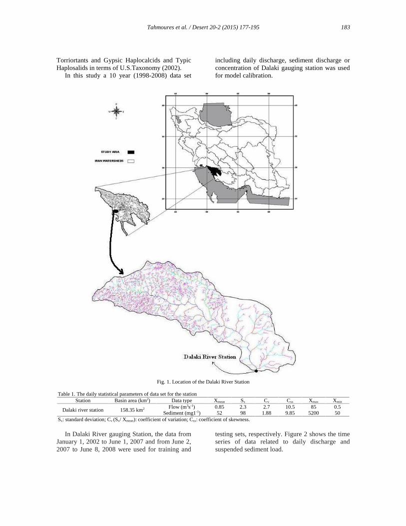
Dalaki River Basin, located in southern Iran wasselected for the study, with Dalaki as the mainriver in the water shed. It has a catchment area of158.35 km2 and lies between 27 07 52 and 3001 02N latitude and 50 01 06 and 52 4506E longitudes (Fig. 1). The area consists ofhills and alluvial plains, with sedimentary geologyincluding Gori limestone, Aghajari marl,Bakhtiyari conglomerate and Quaternary alluviumbased on a 1:100,000 available geologicalmapping. It has a slope range from 5.2 to 15.2%,with an average watershed of 8.2 %. The elevationof the watershed ranges from 50 m to 90 m abovemean sea level. The daily mean temperatureranges from a maximum of 43C to a minimum of3C, and the mean annual temperature is 18.5C.

An arid climate dominates this area, with anannual average rainfall of 150 mm and relative airhumidity of 52%. Generally, it is characterizedwith about 80% of precipitation falls in 2-3intense storm events, with is normallypredominant towards the end of autumn andwinter, with a high temporal and spatial variabilitytypical of such arid regions. All streams areseasonal and require 8 mm/min of rainfallintensity to generate runoff. Table 1 represents thestatistical parameters of streamflow and sedimentconcentration data of Dalaki station.

Land uses comprised Rangeland, uncultivatedlands without vegetation cover, desert pavement,urban area and cropland. The dominant nativeplants are Seidlitzia florida, Artemisia sieberi,Salsola sp, Alhagi camelorum and Halocnemumstrobilaceum. The main soil types are Lithic


Torriortants and Gypsic Haplocalcids and TypicHaplosalids in terms of U.S.Taxonomy (2002).

In this study a 10 year (1998-2008) data set

including daily discharge, sediment discharge orconcentration of Dalaki gauging station was usedfor model calibration.

Fig. 1. Location of the Dalaki River Station

Table 1. The daily statistical parameters of data set for the stationStation Basin area (km2) Data type Xmean Sx Cv Csx Xmax Xmin

Dalaki river station 158.35 km2 Flow (m3s-1) 0.85 2.3 2.7 10.5 85 0.5Sediment (mg1-1) 52 98 1.88 9.85 5200 50

Sx: standard deviation; Cv (Sx/ Xmean): coefficient of variation; Csx: coefficient of skewness.

In Dalaki River gauging Station, the data fromJanuary 1, 2002 to June 1, 2007 and from June 2,2007 to June 8, 2008 were used for training and

testing sets, respectively. Figure 2 shows the timeseries of data related to daily discharge andsuspended sediment load.


Fig. 2. River discharge and suspended sediment load time series (6 years) for Dalaki River Station

4. Data preparation and standardization

Out of the 101 data sets available for the runoffrate and sediment yield in 5 years, about 60%were used for ANN model development while theremaining 40% (≈40 sets) were used for modelvalidation. Of the data used for modeldevelopment, 60% (≈30 sets) were used fortraining while 40% (≈20 sets) were used formodel testing. The Neural Works Professional II +version 5.23 and Neural Network toolbox ofMATLAB 6.5 tools were used in developing theANN models.

5. Estimation of geomorphologic parameters

The present study utilized selectedgeomorphologic parameters of the watershed(Table 1) in developing development the GANNmodels. An estimation of geomorphologicparameters of the study area was made using amap scale of 1:100000 and Strahler ´s orderingsystem (Schuller, 1999). The value of RA, RB, andRL lie in the ranges usually found in naturalwatersheds.

Table 2. Geomorphologic parameters estimated for Dalaki River BasinGeomorphologic parameter Dalaki

BasinPerimeter (km) 138.2Area (km2) 156.6Maximum length (km) 42.3Maximum elevation (m) 90Minimum elevation (m) 50Watershed relief (km) 0.05Relief ratio 0.008Relative relief 0.005Elongation ratio 0.745Mean slope (%) 8.2 %Stream characteristics (Strahler,s stream ordering system) Number of

streamsLength(km)

Area(km2)

Meanlength (km)

Mean area(km2)

1st order streams 52 19.56 45.8 0.78 0.5642nd order streams 23 36.24 65.6 1.78 1.6343rd order streams 6 10.12 18.4 2.56 6.3544th order streams 2 4.68 8.4 2.92 18.54Horton,s parameters RL=2.765 RB=4.655 RA=5.263Total length of streams of all orders (km) 85.5Stream frequency of the watershed (km-2) 3.445Drainage factor of the watershed 0.80Basin Shape factor 1.658Form factor 0.405Circulatory ratio 0.652Drainage density (km-1) 1.652Ruggedness number 0.065Hypsometric integral (Hsi) 0.46


6. Models application

6.1. Sediment Rating Curve (SRC)

Different methodologies have been applied todaily data to derive sediment rating curves atDalaki River gauge. The regression coefficients aand b were calculated by a least squaresregression on the logarithms of discharge and

suspended sediment concentration. Two ratingrelationships were developed using data setgrouped according to seasons. The two regressionlines were almost parallel. For a given discharge,the value of concentration in summer was lowerthan in winter. This concentration variation arosefrom the presence of vegetation cover during thesummer season which protected the soil fromerosion (Fig. 3).

Fig. 3. Sediment rating curves for Dalaki River gauge

6.2. Multi Linear Regression

A comparison of other models with the developedmodel was made using the regression model (Eq.3), Tahmoures, 2008). In this research, variousmorphological catchment properties, land use andsoil texture were analyzed to explain the largevariability in sediment yield. In most cases, astepwise linear regression technique wasapplied. The following models explained mostof the variation in observed sediment yield,having the multi-co linearity betweenindependent variables kept to an acceptableminimum:

ln SSY (t ha-1 year-1) = 4.25 – 0.66 ln A – 0.81 ln HI + 0.11ln Df

(9)SY (g/l) = 0.32 Rr + 18.6 HI + 10.6 Sf – 325 Df

where SSY= specific sediment yield (t ha-1 year-

1); A= catchment area (ha); HI= hypsometricintegral; Df= Drainage factor; SY= sedimentyield (g/l); Rr = Relief ratio; Sf= Basin Shapefactor. The model which predicts SSY explains82% of the observed variability, whereascatchment area alone already explains 66%. ForSY, catchment area is not part of the model,which explains 92% of the observed variation.

6.3. Application of ANNs to data

The four dimensionless geomorphologicalparameters used in Eq. (3) (Table 1) weremathematically associated with the observedrunoff rate as R which were inputted to the ANNmodel in order to develop the GANN.In thisstudy, two algorithms written in MATLAB for


feed-forward back-propagation (FFBP) andradial basis functions (RBF) were employed forANN simulations. The ANN network structureconsisted of three layers, i.e. input layer, singlehidden layer and output layer. The input layerwas prepared using different combinations ofhydrometeorological data. The application of theANNs to time series data consisted of two steps.The first step was the training of the neuralnetworks. This included daily rainfall and flowdata describing the input and sediment load datadescribing the output to the network in order toobtain the inter-connection weights. Once thetraining stage was completed, the ANNs wereapplied to the testing data. As given in Table 3,approximately 5 years of data were used to trainthe networks and less than one year was used totest it. The training set comprised the first 2500values while the testing set covered the last 550values. It is evident that there are variationbetween the statistics of training and testing datasets. Other configurations have also beenconsidered for training and testing sets. First, 550values were considered for testing and thefollowing 2,500 values constituted the training set.However, the statistics for both sets in thisscenario differed from each other. Other optionssuch as taking the testing data set from the middlepart of the whole series did not make muchmeaning from the point of hydrology, since thefirst part and the last part of the whole seriesconstituted the training data set, which accountedfor its discontinuity. Determining an appropriatearchitecture of a neural network for a particularproblem is an important issue since the networktopology directly affects its computationalcomplexity and its generalization capability. ForFFBP, the number of hidden layers and thenumber of the nodes in the input and hiddenlayers were determined after trying variousnetwork structures. There are several methods toavoid overfitting in ANNs. These methods aresummarized by Giustolisi and Laucelli (2005). Inthe present study, ‘‘Early stopping’’ techniquewas adopted. This technique involved the splittingof the training set into two subsets: the estimationand the validation. In this study, the first 2000values in the training set were considered forestimation and the last 500 for validation. Themean square error (MSE) was computed at eachtraining step by means of the validation subset,

while the search direction was computed bymeans of estimation subset. The training stoppedas soon as the validation error rate increased. Thismethod was also used in determining the iteration.Accordingly, for FFBP training experiments, theiteration number was found as 150. Initially,weight values were assigned normally distributednumbers in the interval (-3, +3). A tangentsigmoid function was used as a transfer function.Learning and momentum rate parameters areadaptive, i.e. they change during the training stagedynamically. In the presented study, adaptive(variable) learning rate was used throughout thesimulations. The learning rate values varied from0 to 1. The performance of the algorithm is verysensitive to the proper setting of the learning rate.A relatively high learning rate results inoscillation and instability of the algorithm,similarly, a relatively low learning rate results inan increase in the time for convergence of thealgorithm. It is not practical to determine theoptimal setting for the learning rate beforetraining, and, in fact, the optimal learning ratechanges during the training process, as thealgorithm moves across the performance surface.An adaptive learning rate will attempt to keep thelearning step size as large as possible whilekeeping the learning stable. The learning rate ismade responsive to the complexity of the localerror surface. First, the initial network output anderror are calculated. At each epoch, new weightsand biases are calculated using the currentlearning rate, followed by the calculation of newoutputs and errors. If the new error exceeds theold error by more than a predefined ratio, the newweights and biases are discarded (by multiplyingwith 0.7). In addition, the learning rate isdecreased. Otherwise, the new weights, etc., areretained. If the new error is less than the old error,the learning rate is increased (by multiplying with1.05). This procedure increases the learning rate,but only to the extent that the network can learnwithout large error increament. Thus, a near-optimal learning rate is obtained for the localterrain. A resultant stable learning from an largelearning rate consequently increased the rate oflearning. However, a more than proportionalincrease in learning rate, which cannot guarantee adecrease in error, results in a correspondingdecrease in learning until it attains stability.


Table 3. Training and testing periods for different ANN applicationsStudy type

Simulation I Simulation II Simulation IIITraining 01.01.2002-01.06.2007 01.01.2002-01.06.2007 01.01.2002-01.06.2007Testing 02.06.2007-08.06.2008 02.06.2007-08.06.2008 02.06.2007-08.06.2008

Hidden layer unit number was found separatelyfor each of the input layer scenarios. In order tocircumvent the local minima problem faced inFFBP simulations, many repetitions of the sameFFBP configuration have been made.Accordingly, the FFBP repetition number wasfound as 20 for Simulation I, 18 for Simulation IIand 25 for Simulation III studies. The experimentwith the lowest MSE in testing set was consideredas the representative FFBP simulation. Theexamination of the cross-correlations betweendifferent hydrometeorological series providedpreliminary information regarding the number ofthe nodes in the input layer. It was shown that adetailed preliminary statistical analysis of the datasheds light to the structure of the ANN input layer(Sudheer et al., 2002; Cigizoglu, 2005a). ForRBF, the same input layer structure with FFBPwas employed. Several iteration numbers varyingfrom 5 to 100 were tested. The iteration numberequals to 35 provided best performance criteria.Various spread values between 0 and 1 wereconsidered for RBF simulations. The spreadsproviding best performance criteria for each RBFconfiguration are given in Table 5. The input and

output data were scaled between 0.1 and 0.9 toovercome problems associated with upper-limitand lower-limit saturation. The performanceevaluation measures were the mean square error(MSE) and the coefficient of determination (R2)between simulated and observed sediment loads.However, in the selection of the most appropriateANN configuration, MSE had the priority in thedecision making. But in general, the R2 valueswere in harmony with MSE values. An additionalevaluation criterion, total sediment load of thewhole testing period, was also considered. Thiscomparison in accumulated sediment load playsan important role in reservoir management(especially when considering an annual load). Thesimulation experiments were carried out in threesteps: the first step involved simulating suspendedsediment load data using rainfall measurements asinput; followed by simulating suspended sedimentload data using only flow data as input; andfinally simulating suspended sediment load datausing both rainfall and flow data as input.Conventional multi-linear regression was alsoapplied to the same data for the purpose ofcomparison.

Table 4. The cross-correlations between two different hydrometeorological seriesRainfall (mm)-sediment (tons/day) Flow (m3/s)-sediment (tons/day) Rainfall (mm)- flow (m3/s)

rx,y,0 0.289 0.655 0.185rx,y,1 0.389 0.370 0.390rx,y,2 0.229 0.159 0.403rx,y,3 0.89 0.097 0.335

6.4. Suspended sediment load estimation usingANFIS technique

Adaptive NF model is applied as an effectiveapproach in handling nonlinear and noisy data,especially in situations where the relationshipsamong physical processes are not fullyunderstood. It is also particularly well suited formodeling complex systems on real time basis. Theaim of this research was to investigate theefficiency of ANN and ANFIS models forpredicting suspended sediment load a day ahead.With respect to the statistical analysis presented inTable 6, the following combinations, including

daily stream flow and rainfall of current andprevious days, and suspended sedimentconcentration of previous days, are tried usingANFIS model to estimate current suspendedsediment concentration. The input combinationsused in this application to estimate suspendedsediment concentrations for the Dalaki Riverstation are (i) Qt; (ii) Qt, and Qt_1; (iii) Qt, Qt_1,and Qt_2; (iv) Qt, Qt_1, and St_1; (v) Qt, Qt_1, St_1

and St_2; (vi) Qt, Qt_1, St_1, St_2 and St_3; (vii) Qt,Qt_1, St_1, St_2 and Rt and (viii) Qt, Qt_1, St_1, St_2,Rt and Rt_1, where Qt, St and Rt represent thestream flow, sediment concentration and rainfallat day t, respectively.


Table 5. The performance criteria (MSE and coefficient of determination) values for ANNs obtained for the testing periodsANN model inputs FFBP RBF GANN

Nodes inhidden layer

MSE(tons2/day2)

R2 S (spreadparameter)

MSE(tons2/day2)

R2 Nodes inhidden layer

MSE(tons2/day2)

R2

Rt (Simulation I) 4 657 102 0.018 0.5 653 849 0.025 3 162 749 0.873Rt, Rt_1 (Simulation I) 3 631 230 0.098 0.7 627 231 0.095 6 151 863 0.864Rt, Rt_1, Rt_2 (Simulation I) 1 566 536 0.136 0.8 578 496 0.150 1 122 463 0.861Rt, Rt_1, Rt_2, Rt_3 (Simulation I) 3 520 490 0.213 0.7 562 128 0.174 3 123 672 0.871Rt, Rt_1, Rt_2, Rt_3, Rt_4 (Simulation I) 6 567 071 0.120 0.4 599 258 0.159 5 127 659 0.870Qt (Simulation II) 1 162 749 0.813 0.6 141 956 0.819 5 83 245 0.786Qt, Qt_1 (Simulation II) 3 151 863 0.827 0.5 136 739 0.836 5 111 619 0.873Qt, Qt_1, Qt_2 (Simulation II) 5 122 463 0.873 0.3 115 439 0.878 3 162 749 0.864Qt, Qt_1, Qt_2, Qt_3 (Simulation II) 5 123 672 0.864 0.3 122 976 0.869 3 123 672 0.861Qt, Qt_1, Qt_2, Qt_3, Qt_4 (Simulation II) 5 127 659 0.861 0.3 121 845 0.870 4 162 749 0.871Rt, Rt_1, Rt_2 and Qt (Simulation III) 3 83 245 0.871 0.2 86 122 0.913 3 151 863 0.873Rt, Rt_1, Rt_2, Qt and Qt_1 (Simulation III) 3 111 619 0.870 0.3 92 189 0.905 3 122 463 0.864Rt, Rt_1, Rt_2, Qt, Qt_1 and Qt_2 (Simulation III) 4 117 432 0.786 0.2 97 665 0.889 4 123 672 0.861Rt, Rt_1, Qt and Qt_1 (Simulation III) 3 65 984 0.897 0.3 59 485 0.921 5 127 659 0.871

Table 6. The statistical parameters of data set for the stationData set Data type xmean Sx Cv (Sx/xmean) Csx xmax xmin xmax / xmean

TrainingFlow (m3/s) 18.6 23.7 1.31 3.68 85 0.5 8.96Sediment (t) 1567 5430 4.77 10.43 85.77 3.5 65.8

TestingFlow (m3/s) 16.2 16.8 1.05 1.88 44 0.8 5.66Sediment (t) 1460 2431 2.84 5.33 32.66 14.65 11.48


The ANFIS models were tested and the resultswere compared by means of RMSE, MAE and R2

statistics. The RMSE, MAE and R2 statistics ofeach ANFIS model in test period are given inTable 7. The final architectures of the ANFISmodels found after many trials are also providedin this table. Table 7 indicates the number ofmembership functions of each input variable. Twomembership functions are found to be sufficientfor the suspended sediment estimation. FromTable 7, it is seen that the ANFIS model whoseinputs are current stream flow and rainfall, oneprevious stream flow and two previous suspendedsediment values has the lowest RMSE value (214mg/l). However, the ANFIS model comprisinginput combination (v) has the highest R2 value(0.907). Note that the R2 term providesinformation for linear dependence betweenobservations and corresponding estimates.Therefore, it is not always expected that R2 is inagreement with performance criteria such as theRMSE. For example, in the case of two timeseries such as (Xi = 1,2,3, . . .,10; Yi = 20,40, 60,.. .,200) the R2 between these two series is equal to1 whereas the RMSE value is quite high. An R2

value equal to 1 does not guarantee that a modelcaptures the behavior of the investigated timeseries. In the present study, the main modelperformance criterion is the RMSE. The bestmodel is selected by considering this criterion.Accordingly, it can be said that the ANFIS modelwhose inputs are the Qt, Qt_1, St_1, St_2, and Rt

performs the best among the eight inputcombinations in Table 7. The first threecombinations use the stream flow inputs. In themodels where only stream flows are the inputs,the ANFIS model whose inputs are the currentand one previous stream flow (input combination(ii)) has the best accuracy from the RMSE, MAEand R2 viewpoints. It was observed that theinclusion of 2-day previous stream flow in themodel (input combination (iii)) reduced the modelperformance. Input combinations (iv)–(vi) wereobtained by adding the previous suspendedsediment values into the input combination (ii).An improvement in the simulation performance isexpected by adding the previous suspendedsediment values into the input combinations, sincethe flow measurements are taken together with thesuspended sediment values at the same cross-section of the river (Alp and Cigizoglu, 2007). Inthe models comprising both stream flows andsuspended sediments as the inputs, the ANFISmodel whose inputs are the current and oneprevious stream flow and two previous suspendedsediments (input combination (v)) had the bestaccuracy according to the RMSE, MAE and R2

statistics. Input combinations (vii) and (viii) wereobtained by adding the rainfall values into theinput combination (v). It is evident that theinclusion of 1-day previous rainfall in the model(input combination (viii)) reduced the modelperformance.

Table 7. The final architectures and RMSE, MAE and R2 statistics of the ANFIS models for the test phase

NF model inputsNF structure (number ofmembership functions)

RMSE (mg/l) MAE (mg/l) R2

(i) Qt 6 gauss 282 110 0.819(ii) Qt, Qt_1 2 and 2 gauss 242 82 0.892(iii) Qt,Qt_1, Qt_2 2, 2 and 2 triangular 276 94 0.850(iv) Qt, Qt_1, St_1, 2, 2 and 2 triangular 227 68 0.875(v) Qt,Qt_1, St_1, St_2 2, 2, 2 and 2 triangular 223 58 0.907(vi) Qt, Qt_1, St_1, St_2, St_3 2, 2, 2, 2 and 2 triangular 248 64 0.836(vii) Qt, Qt_1, St_1, St_2, Rt 2, 2, 2, 2 and 2 triangular 214 60 0.890(viii) Qt, Qt_1, St_1, St_2, Rt, Rt_1 2, 2, 2, 2, 2 and 2 triangular 252 71 0.770

A comparison of the ANFIS model with theFFBP, RBF, GANN, MLR and SRC models isseen in Table 8. From that the table, the GANNmodel had the smallest RMSE (55 mg/l) andMAE (17 mg/l) and the highest R2 (0.995) for thetraining phase. In the test phase, however, theANFIS model had the smallest RMSE (215 mg/l)and MAE (58 mg/l) and the highest R2 (0.905).The GANN model also had better accuracy thanthe other ANN approaches. There was consistencyin training and test phase in the GANN. From the

table, it can be deduced that the GANN modelmemorizes the training data. All the ANN modelshad better performances than the SRC model inboth training and test periods.

The sediment peak-estimates obtained by themodels and the corresponding observed values arecompared in Table 9. From the table, the ANFISmodel’s peak-estimates were much closer to theobserved values than those of FFBP, RBF,GANN, MLR and SRC models. All modelsunderestimated the peak values. The ANFIS had


the best accuracy (4) and the SRC had the worstaccuracy (29) in terms of mean absolute relative

errors (MARE) statistics of the peak-sedimentvalues.

Table 8. The training and testing performances of the ANFIS, FFBP, RBF, GANN, MLR and SRC models in suspended sedimentestimation

Models Training phase Test phaseRMSE (mg/l) MAE (mg/l) R2 RMSE (mg/l) MAE (mg/l) R2

ANFIS 154 51 0.965 215 58 0.905FFBP 110 64 0.987 253 71 0.889RBF 178 78 0.963 279 88 0.873

GANN 55 17 0.995 225 62 0.894MLR 188 75 0.885 309 103 0.745SRC 235 108 0.867 325 112 0.739

Table 9. The comparison of the ANFIS, FFBP, RBF, GANN, MLR and SRC peak-estimations for the test phaseObserved

sediment peak(>500 mg l-1)

ANFIS FFBP RBF GANN MLR SRCRelative error (%)

ANFIS FFBP RBF GANN MLR SRC

592 570 537 488 561 455 490 -4 -11 -22 -6 -30 -21612 574 564 478 567 498 445 -7 -9 -28 -8 -23 -38655 599 601 524 674 455 500 -9 -9 -25 3 -44 -31731 745 870 866 768 544 910 2 16 -35 5 -35 20836 795 555 651 784 687 461 -5 -5 -29 -7 -21 -82871 856 564 534 819 598 604 -2 -54 -63 -6 -46 -45920 890 825 801 857 715 765 -4 -12 -15 -8 -29 -21990 973 919 909 945 1150 1130 -2 -8 -9 -5 14 13

1050 1035 988 974 1015 918 920 -2 -7 -8 -4 -15 -151100 1085 1174 1008 1165 1004 1185 -2 7 -10 6 -10 81150 1180 1247 1202 1125 1015 1195 3 8 5 -5 -14 381175 1155 1098 1352 1150 1482 1298 -2 -7 13 -2 21 10

MARE(%)

4 13 22 6 26 29

The estimation of total sediment load obtainedfrom the estimated suspended sedimentconcentration values was also considered forcomparison due to its importance in reservoirmanagement. Table 10 displays the total estimatedsediment amounts in test period. An estimatedtotal sediment load of 810.25 ton according to TheANFIS model was 775.48 ton, with anunderestimation of 4.2%, while the FFBP, RBF,GANN, MLR and SRC models, respectively,computed total sediment load as 668.11, 610.33,735.24, 587.89 and 514.55 ton, withunderestimations of 17.5%, 24.6%, 9.2%, 27.4%and 36.5%, respectively. The estimate of theANFIS model was closest to the observed value.SRC model had the worst estimate. GANN modelhad the best result compared with the other ANNmodels.

The results were also tested by using one-wayanalysis of variance (ANOVA) and t-test for

verifying the robustness (the significance ofdifferences between the model estimates andobserved values) of the models. Both tests wereset at a 95% significant level.

Differences between observed and estimatedvalues were considered significant when theresultant significance level (p) was lower than the0.05 value by use of two-tailed significancelevels. The statistics of the tests are given in Table11. The ANFIS model produced the smallesttesting values (0.3531 and 0.5983) with thecorresponding highest significance level (0.5641)for the ANOVA and t-test, respectively.According to the test results, it is obvious that theANFIS is more robust (the similarity between theobserved suspended sediments and ANFISestimates are significantly high) in estimatingsuspended sediment concentration than the othermethods. The GANN and FFBP models are betterthan the RBF, MLR and SRC.

Table 10. Estimated total sediment amounts in test periodObserved ANFIS FFBP RBF GANN MLR SRC

Estimate (ton) 810.25 775.48 668.11 610.33 735.24 587.89 514.55Relative error (%) 4.2 17.5 24.6 9.2 27.4 36.5


Table 11. Analysis of variance and t-test for suspended sediment concentrationMethod ANOVA t-Test

F-statistic Resultant significance level t-statistic Resultant significance levelANFIS 0.3531 0.5641 0.5983 0.5641FFBP 0.6049 0.4448 0.7041 0.4331RBF 2.5217 0.1181 1.5617 0.1179

GANN 0.4432 0.5732 0.6082 0.5502MLR 3.0042 0.1237 2.6687 0.1189SRC 7.1106 0.0075 2.6874 0.0071

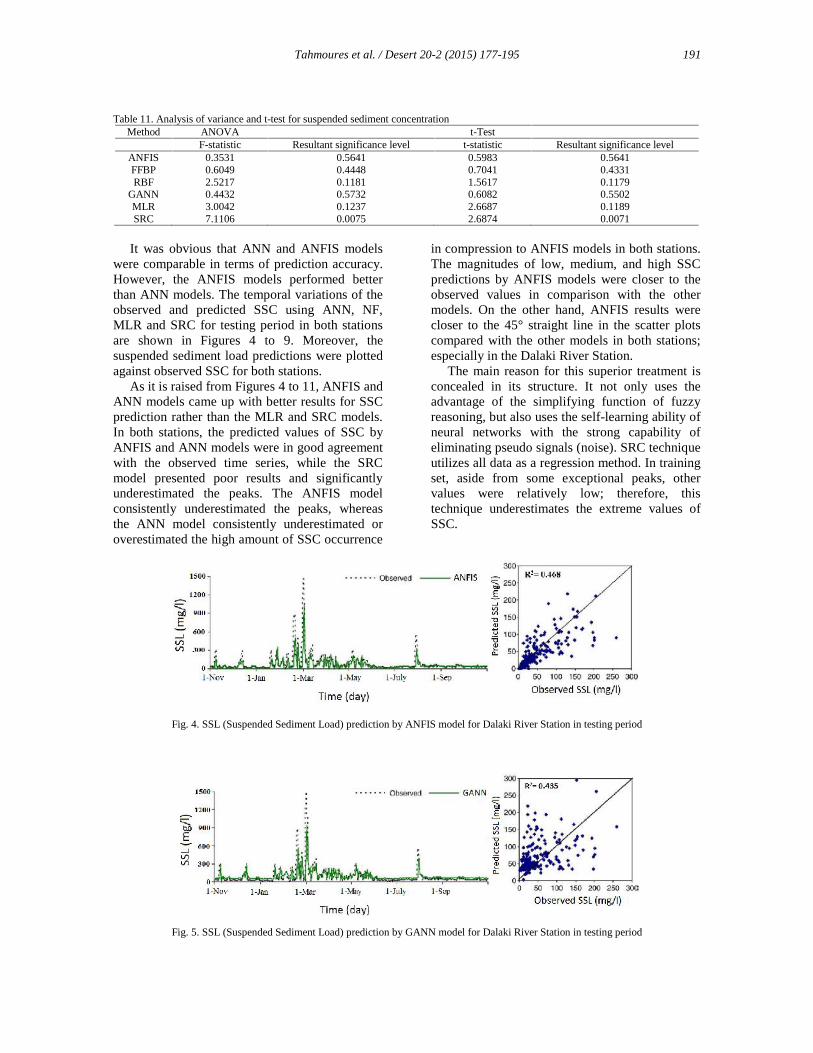
It was obvious that ANN and ANFIS modelswere comparable in terms of prediction accuracy.However, the ANFIS models performed betterthan ANN models. The temporal variations of theobserved and predicted SSC using ANN, NF,MLR and SRC for testing period in both stationsare shown in Figures 4 to 9. Moreover, thesuspended sediment load predictions were plottedagainst observed SSC for both stations.

As it is raised from Figures 4 to 11, ANFIS andANN models came up with better results for SSCprediction rather than the MLR and SRC models.In both stations, the predicted values of SSC byANFIS and ANN models were in good agreementwith the observed time series, while the SRCmodel presented poor results and significantlyunderestimated the peaks. The ANFIS modelconsistently underestimated the peaks, whereasthe ANN model consistently underestimated oroverestimated the high amount of SSC occurrence

in compression to ANFIS models in both stations.The magnitudes of low, medium, and high SSCpredictions by ANFIS models were closer to theobserved values in comparison with the othermodels. On the other hand, ANFIS results werecloser to the 45° straight line in the scatter plotscompared with the other models in both stations;especially in the Dalaki River Station.

The main reason for this superior treatment isconcealed in its structure. It not only uses theadvantage of the simplifying function of fuzzyreasoning, but also uses the self-learning ability ofneural networks with the strong capability ofeliminating pseudo signals (noise). SRC techniqueutilizes all data as a regression method. In trainingset, aside from some exceptional peaks, othervalues were relatively low; therefore, thistechnique underestimates the extreme values ofSSC.

Fig. 4. SSL (Suspended Sediment Load) prediction by ANFIS model for Dalaki River Station in testing period

Fig. 5. SSL (Suspended Sediment Load) prediction by GANN model for Dalaki River Station in testing period


Fig. 6. SSL (Suspended Sediment Load) prediction by FFBP model for Dalaki River Station in testing period

Fig. 7. SSL (Suspended Sediment Load) prediction by RBF model for Dalaki River Station in testing period

Fig. 8. SSL (Suspended Sediment Load) prediction by MLR model for Dalaki River Station in testing period

Fig. 9. SSL (Suspended Sediment Load) prediction by SRC model for Dalaki River Station in testing period

7. Conclusion

In the current study, suspended sedimentconcentrations were estimated by an adaptive

neuro-fuzzy and three different neural networkapproaches using different combinations ofhydrometeorological variables (stream flow andrainfall) and antecedent suspended sediment


concentrations. The first section of study dealtwith the use of several input combinations,including daily stream flow and rainfall of currentand previous days and suspended sedimentconcentration of previous days as inputs to theANFIS model to estimate current suspendedsediment concentration. From the results, theANFIS model whose inputs were current streamflow and rainfall, with one previous stream flowand two previous suspended sediment values hadthe best accuracy. In the second part of the study,the accuracy of the ANFIS model was comparedwith three different ANN computing techniques,GANN, FFBP and RBF in order to ascertain thebest input combination obtained in the first part ofthe study. The MLR and SRC models were alsoconsidered for the comparison. The comparisonresults revealed that the ANFIS model performedbetter than the ANN models, MLR and SRCmodels in daily suspended sediment concentrationestimation. The ANN models also provided betterestimates than the MLR and SRC. According tothe SRC models, the suspended sedimentconcentration was related only to the stream flow.However, the current study demonstrated that thecurrent suspended sediment concentration apartfrom being dependent on the stream flow at thecurrent time, was also dependent on the rainfalland suspended sediment concentration at theprevious periods. The main advantages of usingANFIS and ANN methods are their flexibility andability to model nonlinear relationships. Amongthe ANNs methods, in general, the GANN modelwas found to be slightly better than those of theFFBP and RBF methods in setting up suspendedsediment concentration-hydrometeorologicalrelationship.

Overall, the ANFIS model seems to be moreadequate than the ANN models, together with theMLR and SRC for the process of establishing arating relationship between suspended sedimentand flow. Such problems frequently arise in anonlinear manner. When a rating curve is built,the suspended sediment is related only to thecurrent discharge. However, the currentsuspended sediment is not only dependent on thecurrent discharge but also on the previoussuspended sediment and discharges. The mainadvantages of using ANNs are their flexibility andability to model nonlinear relationships.Mathematically, an ANN may be treated as auniversal approximator (ASCE Task Committee,2000). This technique has already become aprospective research area with great potential due

to simple formulation and the ease of application.However, there are some disadvantages of ANNmethod. The network structure is hard todetermine and it is usually determined using a trialand error approach, i.e., sensitivity analysis(ASCE Task Committee, 2000; Kisi, 2004b). Itstraining algorithm has the danger of getting stuckinto local minima, etc. The ability of an ANN toextrapolate is limited when the input values in theprediction phase are far from the domain of thetraining data set. In this sense, an ANN is not verycapable when it comes to extrapolation. An ANNmodel has a major drawback compared tophysically based models, in that a new inputvariable that was not used in the training phasecannot be introduced to the model in theprediction phase, i.e., the number of inputvariables should be the same during the trainingand prediction phases (Sha, 2007; Dogan et al.,2008). On the contrary, the ANFIS modelscombine the transparent, linguistic representationof a fuzzy system with the learning ability of theANN. Therefore, they can be trained to performan input/output mapping just as with an ANN, butwith the additional benefit of being able toprovide the set of rules on which the model isbased. This gives further insight into the processbeing modeled (Sayed et al., 2003).

This observation would be of much use inhydrological modeling studies where estimates ofsediment values are not available. The model canbe integrated as a module in general hydrologicalanalysis models. In order to improve the currentresearch, using the presented techniques to predictthe suspended sediment load on the second, thirdor other following days, and modeling suspendedsediment load process by considering othervariables (e.g. temperature or precipitationintensity) are suggested. Furthermore, as a planfor the study, the presented approaches can beused to simulate monthly and event based SSCtime series.

References

Agarwal, A., R. Singh, S. Mishra, P. Bhunya, 2005. ANN-based sediment yield models for Vamsadhara riverbasin (India). Water SA, 31(1); 95–100.

Agil, M., I. Kita, A. Yano, S. Nishiyama, 2007. Analysisand prediction of flow from local source in a river basinusing a Neuro-fuzzy modeling tool. J Environ Manag,85; 215–23.

Alp, M., H.K. Cigizoglu, 2007. Suspended sediment loadsimulation by two artificial neural network methods


using hydro meteorological data. Environ Model Softw,22; 2–13.

Altun, H., A. Bilgil, B.C. Fidan, 2007. Treatment of multi-dimensional data to enhance neural network estimatorsin regression problems. Expert Syst Appl, 32(2); 599–605.

ASCE Task Committee on the application of ANNs inhydrology, 2000. Artificial neural networks inhydrology, II: hydrologic application. J Hydrol Eng,5(2); 124–37.

Bazoffi, P., G. Baldasarre, S. Vasca, 1996. Validation ofthe PISA2 model for the automatic assessment ofreservoir sediment deposition. In Proceedings of theInternational Conference on Reservoir SedimentDeposition, Albertson M (ed.). Colorado StateUniversity; 519–528.

Bhattacharya, B., R. Price, D. Solomatine, 2005. Data-driven modelling in the context of sediment transport.Phys Chem Earth, 30; 297–302.

Broomhead, D., D. Lowe, 1988. Multivariable functionalinterpolation and adaptive networks. Complex Systems,2; 321-355.

Brown, M., C. Harris, 1994. Neuro-fuzzy adaptivemodelling and control. Upper Saddle River, NewJersey: Prentice-Hall.

Cigizoglu, H.K., 2005. Application of the generalizedregression neural networks to intermittent flowforecasting and estimation. ASCE Journal ofHydrologic Engineering, 10(4); 336e341.

Cigizoglu, H.K., M. Alp, 2006. Generalized regressionneural network in modelling river sediment yield. AdvEng Softw, 37; 63–8.

Dogan, A., H. Demirpence, M. Cobaner, 2008. Predictionof groundwater levels from lake levels and climate datausing ann approach. Water SA, 34(2); 1–10.

Eberhart, R.C., R.W. Dobbins, 1990. Neural Network PCTools: A Practical Guide. Academic Press, San Diego,414 pp.

El-Bakyr, M.Y., 2003. Feed forward neural networksmodeling for KeP interactions. Chaos, Solitions andFractals, 18(3); 995-1000 (Elsevier).

Engelund, F., E. Hansen, 1967. A monograph on sedimenttransport in alluvial streams. Copenhagen: DanishTechnical (Teknisk Forlag).

Ferguson, R.I., 1986. River loads underestimated by ratingcurves. Water Resour Res, 22; 74–6.

Hagan, M.T., M.B. Menhaj, 1994. Training feed forwardtechniques with the Marquardt algorithm. IEEETransactions on Neural Networks, 5(6); 989-993.

Haykin, S., 1994. Neural Networks: a comprehensivefoundation. New York: MacMillan.

Hornik, K., M. Stinchcombe, H. White, 1989. Multilayerfeedforward networks are universal approximators.Neural Netw, 2(5); 359–66.

Azamathulla, H.M., M.C. Deo, P.B. Deolalikar, 2008,Alternative neural networks to estimate the scour belowspillways, Advances in Engineering Software, 39(8);689-698.

Horowitz, A.J., 2008. Determining annual suspendedsediment and sediment-associated trace element andnutrient fluxes. Sci Total Environ, 400; 315–43.

Jain, S.K., 2001. Development of integrated sedimentrating curves using Anns. J Hydraul Eng, 127(1); 30–7.

Jang, J.S.R., 1993. ANFIS: adaptive-network-based fuzzyinference system. IEEE Trans. Sys. Manage andCybernetics, 23(3); 665–685.

Jang, J.S.R., C.T. Sun, 1995. Neuro-fuzzy modelling andcontrol. Proc IEEE, 83; 378–406.

Jang, J.S.R., C.T. Sun, E. Mizutani, 1997. Neuro-fuzzy andsoft computing: a computational approach to learningand machine intelligence. Upper Saddle River, NewJersey, USA: Prentice Hall.

Kim, B., S.E. Lee, M.Y. Song, J.H. Choi, S.M. Ahn, K.S.Lee, et al, 2008. Implementation of artificial neuralnetworks (ANNs) to analysis of inter-taxa communitiesof benthic microorganisms and macroinvertebrates in apolluted stream. Sci Total Environ, 390; 262–74.

Kisi, O., 2004a. River flow modeling using artificial neuralnetworks. Journal of Hydrologic Engineering, ASCE9(1); 60–63.

Kisi, O., 2004b. Multi-layer perceptrons with Levenberg–Marquardt optimization algorithm for suspendedsediment concentration prediction and estimation.Hydrological Sciences Journal, 49(6); 1025–1040.

Kisi, O., 2005. Suspended sediment estimation usingneuro-fuzzy and neural network approaches.Hydrological Sciences Journal, 50(4); 683–696.

Kisi, O., E. Karahan, Z. Sen, 2006. River suspendedsediment modelling using a fuzzy logic approach.Hydrol Process, 20(20); 4351–4362.

Kisi, O., T. Haktanir, M. Ardiclioglu, O. Ozturk, E. Yalcin,S. Uludag, 2008. Adaptive neuro-fuzzy computingtechnique for suspended sediment estimation. Adv EngSoftw, 40; 438–444.

Legates, D.R., G.J. McCabe Jr, 1999. Evaluating the use ofgoodness-of-fit measures in hydrologic andhydroclimatic model validation. Water Resour Res,35(1); 233–241.

Tuan, L.T., T. Shibayama, 2003. Application of GIS toEvaluate Long-Term Variation of Sediment due toCoastal Environment, Coastal Engineering Journal,JSCE, 45(2); 275-293.

Lohani, A.K., N.K. Goel, K.K. Bhatia, 2007. Derivingstage–discharge–sediment concentration relationshipsusing fuzzy logic. Hydrol Sci J, 52(4); 793–807.

Masters, T., 1993. Practical neural network recipes in C++.San Diego (CA): Academic Press.

Mirbagheri, S.A., K.K. Tanji, R.B. Krone, 1988a.Sediment characterization and transport in Colusa BasinDrain. J Environ Eng, 114(6); 1257–73.

Mirbagheri, S.A., K.K. Tanji, R.B. Krone, 1988b.Simulation of suspended sediment in Colusa BasinDrain. J Environ Eng, 114(6); 1274–93.

Nagy, H.M., K. Watanabe, M. Hirano, 2002. Prediction ofload concentration in rivers using artificial neuralnetwork model. J Hydraul Eng, 128(6); 588–95.

Nash, J.E., J.V. Sutcliffe, 1970. River flow forecastingthrough conceptual models part I — a discussion ofprinciples. J Hydrol, 10(3); 282–90.

Nayak, P.C., K.P. Sudheer, D.M. Rangan, K.S. Ramasastri,2004. A neuro-fuzzy computing technique for modelinghydrological time series. Journal of Hydrology, 291(1–2); 52–66.


Nourani, V., A.A. Mogaddam, A.O. Nadiri, 2008. AnANN-based model for spatiotemporal groundwaterlevel forecasting. Hydrol Process, 22; 5054–5066.

Nourani, V., M.T. Alami, M.H. Aminfar, 2009. Acombined neural-wavelet model for prediction ofLigvanchai watershed precipitation. Eng Appl ArtifIntell, 22; 466–472.

Nourani, V., M. Komasi, A. Mano, in press. A multivariateANN-wavelet approach for rainfall-runoff modeling.Water Resources Management, Published online,doi:10.1007/s11269-009-9414-5.

Ocampo-Duque, W., M. Schuhmacher, J.L. Domingo,2007. A neural-fuzzy approach to classify the ecologicalstatus in surface waters. Environ Pollut, 148; 634–641.

Poggio, T., F. Girosi, 1990. Regularization algorithms forlearning that are equivalent to multilayer networks.Science, 2247; 978-982.

Raghuwanshi, N., R. Singh, L. Reddy, 2006. Runoff andsediment yield modeling using artificial neuralnetworks: Upper Siwane River, India. J Hydrol Eng,11(1); 71–79.

Rajaee, T., S.A. Mirbagheri, M. Zounemat-Kermani, V.Nourani, 2009. Daily suspended sediment concentrationsimulation using ANN and neuro-fuzzy models. Scienceof the Total Environment, 407; 4916-4927.

Rajaee, T., V. Nourani, M. Zounemat-Kermani, K. Ozgur,2011. River Suspended Sediment Load Prediction:Application of ANN and Wavelet Conjunction Model .Journal of Hydrologic Engineering, ASCE, 16(8); 613-627.

Raman, H., N. Sunilkumar, 1995. Multivariate modellingof water resources time series using artificial neuralnetworks. Hydrol Sci J, 40(2); 145–63.

Restrepo, J.D., J.P.M. Syvitski, 2006. Assessing the Effectof Natural Controls and Land Use Chane on SedimentYield in a Major Andean River: The MagdalenaDrainage Basin, Colombia. Ambio: a Journal of theHuman Environment, 35; 44-53.

Sahoo, G.B., C. Ray, E. Mehnert, D.A. Keefer, 2006.Application of artificial neural networks to assesspesticide contamination in shallow groundwater. SciTotal Environ, 367; 234–51.

Salas, J.D., J.W. Delleur, V. Yevjevich, W.L. Lane, 1980.Applied modeling of hydrological time series. Denver:Water Resources Publications.

Sarangi, A., A.K. Bhattacharya, 2005. Comparison ofArtificial Neural Network and regression models forsediment loss prediction from Banha watershed in India.Agricultural Water Management, 78; 195–208.

Sayed, T., A. Tavakolie, A. Razavi, 2003. Comparison ofadaptive network based fuzzy inference systems and B-spline neuro-fuzzy mode choice models. WaterResources Research, 17(2); 123–130.

Schuller, B., 1999. Automatisches Verstehen gesprochenermathematischer Formeln. Diploma thesis, TechnischeUniversit¨at M¨unchen, Munich, Germany.

Sha, W., 2007. Comment on: ‘flow forecasting for a

Hawaii stream using rating curves and neuralnetworks’ by G.B. Sahoo and C. Ray. Journal ofHydrology 340 (1–2), 119–121. Journal of Hydrology,317; 63–80.

Sinnakaudan S.K., A.A.B. Ghani, M.S.S, Ahmad, N.A.Zakaria, 2006. Multiple linear regression model for totalbed material load prediction. Journal of HydraulicEngineering, 132(5); 521-528.

Tahmoures, M., A. Karimi, 2008. Estimation of DailySuspended Sediment Yield Based on Neural Networksand Neuro-Fuzzy Technique, Pajouhesh-va-sazandegiJournal, 21; 61–75.

Taurino, A.M., C. Distante, P. Siciliano, L. Vasanelli,2003. Quantitative and qualitative analysis of VOCsmixtures by means of a microsensors array and differentevaluation methods. Sensors and Actuators, 93; 117-125.

Tay, J.H., X. Zhang, 1999. Neural fuzzy modeling ofanaerobic biological wastewater treatment systems.J.Environ, 125(12); 1149-1159.

Tayfur, G., S. Ozdemir, V.P. Singh, 2003. Fuzzy logicalgorithm for runoff-induced sediment transport frombare soil surfaces. Adv Water Resour, 26; 1249–1256.

Tokar, A.S., P.A. Johnson, 1999. Rainfall runoff modellingusing artificial neural networks. J Hydrol Eng, 4(3);232–239.

Tsai, C.H., L.C. Chang, H.C. Chiang, 2009. Forecasting ofozone episode days by cost-sensitive neural networkmethods. Sci Total Environ, 407; 2124–35.

Vanacker, V., M. Vanderschaeghe, G. Govers, E. Willems,J. Poesen, J. Deckers, B. De Biévre, 2009. Linkinghydrological, infinite slope stability and land use changemodels through GIS for assessing the impact ofdeforestation on landslide susceptibility in high Andeanwatersheds. Geomorphology, 52; 299-315.

Verstraeten, G., J. Poesen, 2001. Factors controllingsediment yield fromsmall intensively cultivatedcatchments in a temperate humid climate.Geomorphology, 40; 123–44.

Williams, G.P., 1989. Sediment concentration versus waterdischarge during single hydrologic events in rivers. JHydrol, 111(1–4); 89–106.

Yang, C.T., 1996. Sediment transport, theory and practice.New York: McGraw-Hill.

Zhu, Y.M., X.X. Lu, Y. Zhou, 2007. Suspended sedimentflux modeling with artificial neural network: anexample of the Longchuanjiang River in the UpperYangtze Catchment, China. Geomorphology, 84; 111–25.

Zounemat-Kermani, M., M. Teshnehlab, 2008. Usingadaptive neuro-fuzzy inference system for hydrologicaltime series prediction. Appl Soft Comput, 8; 928–936.

Zounemat-Kermani, M., A.A. Beheshti, B. Ataie-Ashtiani,S.R. Sabbagh-Yazdi, 2009. Estimation of current-induced scour depth around pile groups using neuralnetwork and adaptive neuro-fuzzy inference system.Appl Soft Comput, 9; 746–55.

modeling of streamflow-suspended sediment load ... · from the results, adaptive neuro-fuzzy...

Documents