modeling preference data - ub

Abstract We provide a gentle overview of modeling choice data, with an emphasis on statistical models that allow treating both observed and unobserved effects due to the decision makers and choice options. We first consider the situation when decision makers express their preferences in the form of liking judgments or purchase intentions (as in conjoint studies).Then, we consider applications that involve partial and/or incomplete ranking data –including paired comparisons and first choices. In this case, we assume that choice outcomes are a result of a maximization process, i.e., decision makers are assumed to select or choose options that have the highest utility among the considered options. These utilities are not observed but can be inferred, at least partially, from the choices observed under the maximization assumption.

Keywords Preference data, random utility models, conjoint analysis, political preferences, vocational interests

MODELING PREFERENCE DATA

IE Business School Working Paper WP08-30 31-10-2008

Alberto Maydeu-Olivares Ulf Böckenholt

McGill University Faculty of Management

1001 Sherbrooke St. West, Montreal, Québec - Canada

H3A 1G5 [email protected]

IE Business School Marketing Dept.

C/ Maria de Molina, 11-15 28006, Madrid – Spain

[email protected]

IE Business School working Paper WP08-30 31-10-2008

1

Introduction

A great deal of data in management research can be considered the result of a choice

process. Familiar instances are a citizen deciding whether to vote and if so for whom, a

shopper contemplating various brands of a product category, or a physician deciding various

treatment options. Less obvious examples of discrete choices are responses to multiple choice

items of a proficiency test in mathematics or to rating items in a personality questionnaire.

Here, an individual's answers may be viewed as her top choices among the alternatives

presented. Choices may also be expressed in an ordinal and continuous fashion. Instances

include decisions on how much food to consume, how much to invest in the stock market, or

how much to pay in an online auction. Finally, multivariate choices may be observed when

considering, for example, consumers’ choices of brands within different product categories

and their respective quantity purchases.

Choice outcomes may be gathered in either natural or experimental settings. Both

types of outcomes are of interest, as they can often complement one another. They are

referred to as revealed and stated preferences respectively (Louviere et al. 2000). For

instance, in an election, stated preferences (rankings of the candidates shortly before the

election) may prove more useful for predicting the election outcome and provide more

information about the motives than would revealed preferences such as past voting behavior.

As revealed preferences are frequently collected in observational studies, they are more

difficult to interpret in an unambiguous way, and they can also provide considerably less

information than stated preferences. Typically, revealed preferences are first choices. Second-

best option or least-liked option, etc. are less commonly observed, although they may be

critical for accurately forecasting future behavior. Moreover, the collection of stated

preference data is also useful in situations when it is difficult or impossible to collect revealed

preference data because choices are made infrequently, or because new choice options offered

in the studies are yet unavailable on the market. For example, in taste testing studies,

consumers may be asked to choose among existing as well as newly developed products.

Often, standard models can be used to model preference data. However, care needs to

be taken in the selection of an appropriate model because one needs to take into account the

response process that leads to the observed choice data. For example, the choice of a

response category in a mathematics test may be driven by both the abilities of the

respondents and the difficulties of the items. In contrast, the decision on how much to invest

may depend on investment knowledge, the budget available and the respondents’ perception

of risk. In ability testing, much work has focused on the separability of item and person

characteristics leading to item response models. However, in preference analysis, it is

frequently a foregone conclusion that item and person characteristics are not separable. As a

result, statistical tools are needed that can identify how respondents differ in their perception


2

and preferences for a set of choice options (Böckenholt and Tsai, 2006).

The choice models that we consider here include the logistic regression model (Bock,

1969; Luce, 1957; McFadden, 2001) and Thurstone's (1927) class of models for comparative

data in the form of rankings or paired comparisons. Both classes of models are probabilistic

in nature and focus on decision problems with a finite number of options. They allow

predicting how observed and unobserved attributes of both decision makers and choice

options determine decisions. It is important to note that these models focus mainly on choice

outcomes and to a lesser extent on underlying decision processes. As a result, their main

purpose is to summarize the data at hand and to facilitate the forecasting of choices made by

decision makers facing possibly new or different variants of the choice options.

The objective of the present work is to provide a gentle overview of modeling choice

data, with an emphasis on statistical models that allow treating both observed and

unobserved effects due to the decision makers and choice options. Our discussion of how to

model individual differences in the evaluation as well as selection of choice options will

consider first the situation when decision makers express their preferences in the form of

liking judgments or purchase intentions. These types of data are commonly collected in

conjoint studies (Marshall & Bradlow, 2002) which aim at measuring preferences for product

attributes. We will then consider applications that involve partial and/or incomplete ranking

data (Bock & Jones, 1968). Incomplete ranking data are obtained when a decision maker

considers only a subset of the stimuli. For example, in the method of paired comparison, two

stimuli are presented at a time, and the decision maker is asked to select the one she prefers.

In contrast, in a partial ranking task, a decision maker is confronted with all stimuli and

asked to provide a ranking for a subset of the available options. For instance, in the best–

worst method, a decision maker is instructed to select the best and worst options out of the

set of choice options offered.

Both partial and incomplete approaches can be combined by offering multiple distinct

subsets of the choice options and obtaining partial or complete rankings for each of them.

For instance, a judge may be presented with all possible stimulus pairs sequentially and

asked to select the preferred stimulus in each case. Presenting choice options in multiple

blocks has several advantages. First, the judgmental task is simplified since only a few

options need to be considered at a time. Second, as we show later, it is possible to

investigate whether judges are consistent in their evaluations of the stimuli. Third, obtaining

multiple judgments from each decision maker simplifies analyses of how individuals differ in

their preferences for the stimuli, as we illustrate in one of the examples. These advantages

need to be balanced with the possible boredom and learning effects that may affect a

person’s evaluation of the stimuli when the number of blocks is large.

Analyses of partial and/or incomplete ranking data require the additional

specification that choice outcomes are a result of a maximization process. In other words,


3

decision makers are assumed to select or choose options that have the highest utility among

the considered options. These utilities are not observed but can be inferred, at least partially,

from the choices observed under the maximization assumption. Because less information is

available about the underlying utilities in a choice task than in a rating setting, we discuss

interpretational issues in the application of choice models for partial and/or incomplete

ranking data as well.

A basic model for continuous preferences

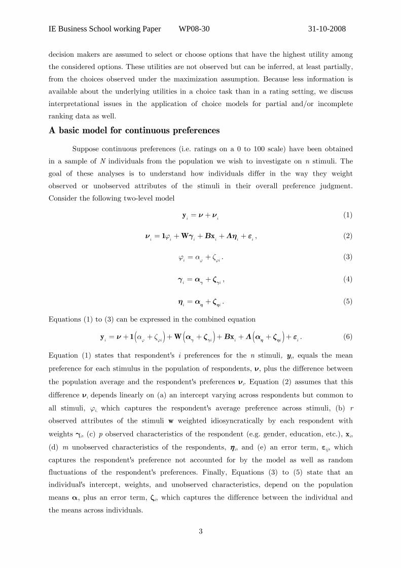
Suppose continuous preferences (i.e. ratings on a 0 to 100 scale) have been obtained

in a sample of N individuals from the population we wish to investigate on n stimuli. The

goal of these analyses is to understand how individuals differ in the way they weight

observed or unobserved attributes of the stimuli in their overall preference judgment.

Consider the following two-level model

i i

ν ν= +y (1)

i i i i i i

ν γ Β Λη ε= + + + +1 W xϕ , (2)

i i= +ϕ ϕϕ α ζ . (3)

i iγ γγ α ζ= + , (4)

i iη ηη α ζ= + . (5)

Equations (1) to (3) can be expressed in the combined equation

( ) ( ) ( )i i i i i iγ γ η ην α ζ Β Λ α ζ ε= + + + + + + + +y 1 W xϕ ϕα ζ . (6)

Equation (1) states that respondent's i preferences for the n stimuli, yi, equals the mean

preference for each stimulus in the population of respondents, ν, plus the difference between

the population average and the respondent's preferences νi. Equation (2) assumes that this

difference νi depends linearly on (a) an intercept varying across respondents but common to

all stimuli, ϕi, which captures the respondent's average preference across stimuli, (b) r

observed attributes of the stimuli w weighted idiosyncratically by each respondent with

weights γi, (c) p observed characteristics of the respondent (e.g. gender, education, etc.), xi,

(d) m unobserved characteristics of the respondents, ηi, and (e) an error term, εij, which

captures the respondent's preference not accounted for by the model as well as random

fluctuations of the respondent's preferences. Finally, Equations (3) to (5) state that an

individual's intercept, weights, and unobserved characteristics, depend on the population

means α, plus an error term, ζi, which captures the difference between the individual and

the means across individuals.


4

The m unobserved characteristics of the respondents are common factors. In turn, the

observed characteristics of the respondents, x, and the observed characteristics of the stimuli,

w, may be metric variables or dummy variables which represent categorical factors. This is a

basic setup for modeling preferences in the sense that it accounts for observed and

unobserved attributes of the decision makers and allows relating attributes of the stimuli to

the overall preference judgment with person-specific regression weights.

Although fairly general, this model can be extended in two important ways. First,

there may be interactions between the respondents’ characteristics, x, between stimuli

attributes, w, or between the respondents’ characteristics and the stimuli attributes.

Especially, the latter effect can be of great interest in preference modeling when investigating

how respondents with different background characteristics differ in terms of the perception

and evaluation of the same choice option. For example, in survey studies on US politicians

involving thermometer ratings (Regenwetter et al., 1999), it is well known that Republican

and Democrat voters may disagree in systematic ways on their evaluation of political

programs endorsed by the politicians.

Second, the relationship between preferences and the respondents’ characteristics and

stimulus attributes may be non-linear. A simple example is the liking of the sweetness of

drink as a function of the number of spoonfuls of sugar used. Too much or too little sugar

may lead to lower likings suggesting a quadratic relationship between these two variables. In

this case, an ideal-point model may prove superior to a linear representation when

individuals choose the option that is closest to their “ideal” or most preferred option

(Böckenholt, 1998; Coombs, 1964; MacKay, Easley, & Zinnes, 1995).

Both extensions can be incorporated straightforwardly in the basic model for the

observed characteristics of the respondents and stimuli. It is therefore instructive to consider

also special cases of Equation (6). A special case is obtained when no information on the

attributes of the stimuli or the observed characteristics of the respondents are available. In

addition, the respondent specific intercept, ϕi, is not generally included in the model – but

see Maydeu-Olivares and Coffman (2006). This leads to

i i i

ν Λη ε= + +y , i iη ηη α ζ= + . (7)

Thus, in this model, preferences among the n stimuli are explained solely by a set of m

unobservable characteristics of the respondents η which leads to a model with m common

factors. The common factors are treated as random effects, and they are assumed to be

uncorrelated with the random errors. The variances of the random errors are assumed to be

equal across respondents within a stimulus, but typically they are allowed to be different

across stimuli. Also, random errors are assumed to be mutually uncorrelated across stimuli,

so their covariance matrix is diagonal. Finally, the means of the random errors and common

factors are specified to be zero.


5

An interesting special case of the factor model is obtained when it is assumed that

the mean preferences depend on the means of the unobserved factors. In the factor analysis

model, ν and αη are not jointly identified. However, αη can be estimated if it is assumed that

the intercepts are equal for all stimuli, υ = 1υ . With this assumption, the population mean

and covariance matrices of the observed preferences are

μ Λα= +1ν , ′= +Σ ΛΨΛ Θ . (8)

The latter expression is the standard formula for the covariance structure of the factor

analysis model where Ψ and Θ denote the covariance matrices of ηζ and ε , respectively.

Another special case of the general model of Equation (6) is obtained when no

information on the stimuli's attributes is available and no unobserved characteristics of the

respondents are specified. Also, the respondent specific intercept, ϕi, is not included in the

model. In this case we have

i i i

ν Β ε= + +y x . (9)

This equation is a multivariate (fixed effects) regression model where the respondents'

characteristics are used to explain the preferences. Typically, the x are assumed to be fixed

and the errors are assumed to be independent with mean zero and common variance within a

stimuli, but variances may be different across stimuli and errors across stimuli may be

correlated.

Finally, when no information on the respondents' characteristics is available and no

unobserved characteristics of the respondents are specified, we have

i i i

ν γ ε= + + +y 1 Wϕ . (10)

One approach to specify model (10) is to treat i

ϕ and γi as random effects, where the

random intercepts i

ϕ and random slopes γi are assumed to be mutually uncorrelated and

uncorrelated with the random errors iε . In this case, Equation (10) is a multivariate

random-effects regression model. As in the common factor model, the mean of the random

errors is specified to be zero and their covariance matrix is assumed to be diagonal. In fact,

the random-effects multivariate regression model is closely related to the common factor

model. The key differences between these two models are that in the random effects

regression model (a) the number of latent factors is fixed, r + 1 (the additional latent factor

is the random intercept), and (b) the factor loadings are fixed constants (given by the n × r

design matrix W). Also, as in the factor analysis model, it is interesting to let the mean

preferences depend on the means of the random intercepts and slopes, ϕα and γα . To do so,

ν must be set to zero for identification, leading to

* *μ α= W , * * *Σ Ψ Θ′= +W W , (11)


6

where ( )* =W 1 W , ( )*γα α= ϕα , *Ψ denotes the covariance matrix of ( ),

i iγ

′′ϕ , and Θ

denotes the covariance matrices of the random errors.

An alternative approach to specify the model (10) is to treat i

ϕ and γi as fixed

effects. Again, in this case ν cannot be estimated, but the parameters of interest, i

ϕ and γi,

can be estimated for each person separately. This approach is taken in classical conjoint

analysis (Louviere, Hensher & Swait, 2000). In this popular technique, preferences are

modeled using (10) with ν = 0 on a case-by-case basis where the r stimuli attributes are

generally expressed as factors (in the analysis of variance sense) using effect coding.

Some remarks on estimation

Structural equation modeling provides a convenient way of estimating the general

model and its special cases presented in this section. Assuming multivariate normality of the

random variables y, estimation may be performed using maximum likelihood. However, it

suffices to assume that the distribution of the observed preferences y conditional on x is

multivariate normal. This assumption enables the inclusion of non-normal exogenous

variables in the model, such as dummy variables (for further technical details see Browne

and Arminger, 1995). When the observed preferences are non-normally distributed,

asymptotically robust standard errors and goodness of fit tests for maximum likelihood

estimates can be obtained – see Satorra and Bentler (1994) for further details.

Numerical example 1: Modeling preferences for a new detergent

Hair et al. (2006) provide ratings of 18 detergents on a 7-point scale ranging from

"not at all likely to buy" to "certain to buy" by 86 customers. We note that although Hair et

al. (2006) report the results obtained using 100 respondents, the dataset available for

download contains only 86 respondents. The detergents were obtained using a fractional

design involving 5 factors:

1. Form of the product (Premixed liquid, concentrated liquid, or powder)

2. Number of applications per container (50, 100, or 200)

3. Addition to disinfectant (yes, or no)

4. Biodegradable (no, or yes)

5. Price per application (35, 49, or 79).

The first, second and fifth attributes of this conjoint analysis consist of 3 levels, whereas the

other attributes consist of 2 levels. With k levels per attribute, only k – 1 are mathematically

independent. Here, arbitrarily, we shall estimate the effects corresponding to the first k – 1

levels. Also, notice that the attributes with 3 levels could be treated metrically, using a

linear or quadratic function, etc. Here, we shall estimate them as ANOVA factors.

Fixed effects modeling: conjoint analysis

If i

ϕ and γi are treated as fixed effects, they can be estimated for each respondent


7

separately. Thus, for each respondent, there are 18 observations and 9 parameters: 1

intercept, 2 parameters each for factors 1, 2 and 5, and 1 parameter for each of the

remaining 2 factors. In conjoint analysis terminology, the predicted responses ˆi

y are called

utilities and the estimated regression (actually ANOVA) parameters ˆi

γ are called part-

worth utilities. In fact, in conjoint analysis part-worth utilities are estimated for all factor

levels using the constraint that all parameters for an attribute within a respondent add up to

zero. Typically, the part-worth utilities are only of secondary interest. Of primary interest

are the importance of each attribute in determining choice and the proportion of times that

an option will be chosen in the population of consumers (see Louviere, Hensher & Swait,

2000 for details on how to compute these statistics).

Here, we shall focus on the parameter estimates. Table 1 provides the means and

variances of the parameter estimates averaged across the individual regressions. No standard

errors are readily available when population means and variances are estimated in this

fashion (but see Bollen and Curran, 2006, pp. 25-33).

−−−−−−−−−−−−−−−−−−−−− Insert Tables 1 and 2 about here

−−−−−−−−−−−−−−−−−−−−− Random effects approach

Alternatively, i

ϕ and γi can be treated as random effects. This multivariate

regression random effects regression model can be estimated as a confirmatory factor-analysis

model where the factor matrix is given by the design matrix employed. In this example, the

design matrix W* for the 18 stimuli is given in Equation (12).

The first column corresponds to the random intercept. Columns 2 and 3 correspond

to the first 2 levels of the first factor, columns 4 and 5 correspond to the first two levels of

the second factor, column 6 to the first level of the third factor, and so on. Notice how effect

coding has been used, as is customary in conjoint analysis. The variances and covariances of

the 9 random effects can be estimated as well as their means if ν = 0 (for identification).

Also, the covariance matrix of the random errors is assumed to be a diagonal matrix. This

two-level regression model can be readily estimated with any software package for structural

equation or multilevel modeling.

Assuming normality of the observations, we obtained by maximum likelihood that

the model fits very poorly, X2 = 270.65 on 117 df, p < .01, the RMSEA (see Browne &

Cudeck, 1993) is 0.12. This is a valuable piece of information, as with the fixed effects

approach we could not obtain an overall assessment of the model’s fit. Rather, we obtained

an R2 for each individual separately (which in most cases ranged from 0.75 to 0.95).


8

*

1 0 1 1 1 1 1 1 0

1 1 1 1 1 1 1 1 0

1 1 0 0 1 1 1 0 1

1 1 1 1 1 1 1 0 1

1 1 1 1 0 1 1 1 1

1 0 1 1 1 1 1 1 1

1 1 0 0 1 1 1 1 1

1 1 0 1 1 1 1 0 1

1 1 1 0 1 1 1 0 1

1 0 1 1 0 1 1 0 1

1 1 1 0 1 1 1 1 0

1 0 1 0 1 1 1 1 1

1 1 0 1 1 1 1 1 1

1 1 0 1 0 1 1 1 0

1 0 1 0 1 1 1 1 0

1 1 0 1 0 1 1 1 0

1 0 1 1 0 1 1 0 1

1

− −− − − −

−− − − − −− − − −

− − − − − −− −

− −− − −

− − −− −

− − − − −

−− −−

=W

1 1 1 0 1 1 1 1

⎛ ⎞⎟⎜ ⎟⎜ ⎟⎜ ⎟⎜ ⎟⎜ ⎟⎜ ⎟⎟⎜ ⎟⎜ ⎟⎜ ⎟⎜ ⎟⎜ ⎟⎜ ⎟⎜ ⎟⎜ ⎟⎟⎜ ⎟⎜ ⎟⎜ ⎟⎜ ⎟⎜ ⎟⎜ ⎟⎜ ⎟⎟⎜ ⎟⎜ ⎟⎜ ⎟⎜ ⎟⎜ ⎟⎜ ⎟⎜ ⎟⎜ ⎟⎟⎜ ⎟⎜ ⎟⎜ ⎟⎜ ⎟⎜ ⎟⎜ ⎟⎜ ⎟⎟⎜ ⎟⎜ ⎟⎜ ⎟⎜ ⎟⎜ ⎟⎜ ⎟⎜ ⎟⎜ ⎟⎟⎜ ⎟⎜ ⎟⎜ ⎟⎜ ⎟⎜ ⎟⎜ ⎟⎜ ⎟⎟⎜ ⎟⎜ ⎟⎜ ⎟⎜ ⎟⎜ ⎟⎜ ⎟⎜ ⎟⎜ ⎟⎟⎜ ⎟⎜ ⎟⎜ − − − − − ⎟⎟⎜⎝ ⎠. (12)

Table 2 provides the estimated population means and variances of i

ϕ and γi. Notice

in this table that the estimated variance for the preferences for concentrated liquid

detergents is very small (0.001) suggesting that individuals vary little in their weight of this

factor. Comparing the parameter estimates across methods (fixed effects vs. random effects),

we see that the estimated means are rather similar. The estimated variances, in contrast,

appear generally larger when estimated on a case-by-case fashion.

The reasons for the discrepancy in the variance estimates are probably three-fold.

First, in view of the large number of parameters that are estimated for each person in the

fixed-effects approach, it is not surprising that the variance estimates are much larger in this

case. Second, the assumption that the random effects are normally distributed constrains the

estimates of the random effects’ variances and covariances. Similar constraints are not in

place when estimating the regression coefficients for each person separately. The multivariate

normality assumption of the random effects may only be partially appropriate for this data

set: The distribution of the fixed-effect estimates of the coefficients for the “addition to

disinfectant” factor appears to be bimodal. However, the distributions of the other

coefficients appear roughly normal, except for a few outliers and some excess kurtosis. Third,

the two methods make different assumptions about the residual error variances. Whereas the

individual-regression approach assumes that the εi are constant across stimuli but different

across respondents, our random-effects model assumes that the εi are constant across

respondents but different across stimuli. This latter specification can be relaxed provided

covariates are available that allow modeling heteroscedasticity effects on the person level.


9

In closing this example, we note that the structural equation modeling of the random-

effects specification facilitates the testing of a number of interesting hypotheses. For

instance, one may test whether the residual errors are correlated for some stimuli. This

consideration of local dependencies may be particularly useful when similarities among

stimuli (caused, for example, by the same presentation formats) cannot be accounted for by

individual differences. Also, replicated stimuli are accommodated easily. Hair et al. (2006)

provide two replicates for each respondent. Modeling both replicates simultaneously using

the random-effects model requires using a 36 × 9 design matrix obtained by duplicating the

matrix in Equation (12).

Numerical example 2: Modeling preferences for Spanish politicians

In our first example, we saw an instance of the basic model where preferences were

modeled as a function of observed characteristics of the stimuli using (10). In this example,

we shall model instead preferences as a function of unobserved characteristics of the

respondents using (7). The Centro de Investigaciones Sociológicas (CIS) of the Spanish

Government periodically obtains a representative national sample of approval ratings on a

scale from 0 to 10 for the Ministers of the Spanish Government along with the leaders of the

opposition parties. Here, we used the October 2004 data and selected the eight politicians

with the lowest amount of missing responses. Using listwise deletion, we obtained a final

sample size of 576. The purpose of this example is to show how unobserved characteristics of

the respondents can be used to predict the average approval rating of each politician. Table

3 shows the average approval ratings for the eight politicians analyzed. As we can see from

this table, the average ratings range from 5.55 to 2.86. The Spanish president at the time of

the study (equivalent to Prime Minister in other political systems), Rodriguez Zapatero,

obtained the highest rating, and the leader of the main opposition party, Rajoy, the fourth

highest rating. The second and third positions are for two ministers of Zapatero's cabinet,

Solbes and Bono. A lower rating is obtained by the leader of a leftist party, Llamazares. Low

ratings are also obtained by the leaders of smaller, regional parties, Duran, Carod and Imaz.

The regional parties these three politicians represent focus on the national identity of the

autonomous regions where their parties operate. The aim of these parties is to increase the

power of their regions with respect to the central Spanish government, in some cases with

the declared objective of achieving independence.

Our model postulates that respondents use a number of unobserved preference

dimensions to rate these politicians. We use a factor-analysis model to uncover these

dimensions. Since the observed ratings are not normally distributed, we used maximum

likelihood with robust standard errors and Satorra-Bentler mean adjusted goodness of fit

statistics. A model with one common factor, which we interpreted as right-left political

affiliation, fits very poorly, Satorra-Bentler (SB) mean adjusted X2 = 801.7 on 20 df,


10

RMSEA = .263. A model with two common factors, which can be interpreted as Centralism-

Peripheralism and Non-nationalism-Nationalism, also fits rather poorly, SB X2 = 114.2 on 13

df, RMSEA = .118. However, a model with three dimensions cannot be rejected at the 5%

significance level, SB X2 = 13.8 on 7 df, p = .05, RMSEA = .042. Next, we constrain the

mean ratings to depend on the common factors, while estimating the factor means. That is,

according to this model, the population mean and covariance matrices are given by Equation

(8).

The model fits the data adequately: SB X2 = 24.2 on 11 df, p = .01, RMSEA = .046,

and yields interesting insights into the individual differences underlying the ratings of the

politicians. The factor loadings for this mean-structured factor model are provided in Table

3. In this model, the factor loadings represent the position of the politicians in the preference

space of the respondents. A plot of the factor loadings (i.e., a preference map) facilitates the

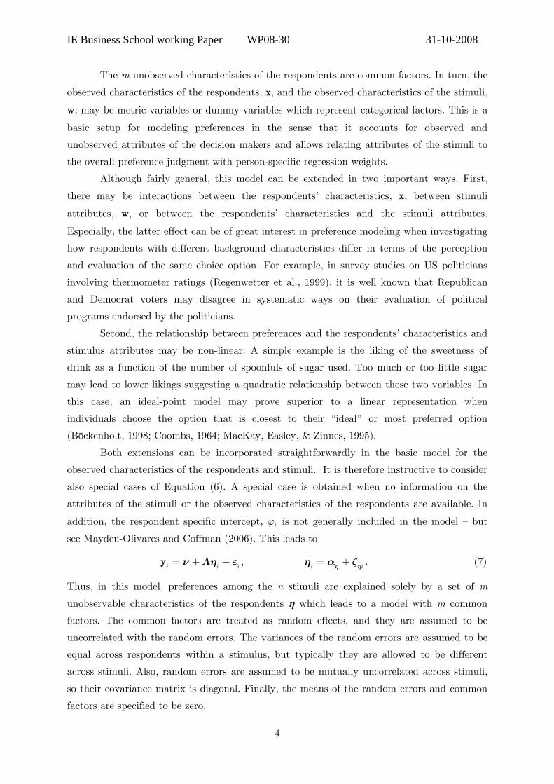
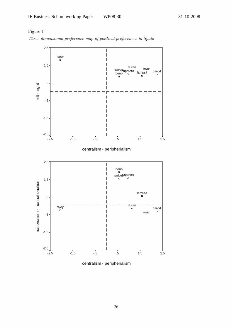
interpretation of the dimensions. The preference map is provided in Figure 1. One of the

dimensions can be interpreted as Centralism- Peripheralism. High scores on this dimension

indicate that politicians are perceived as favoring a weak central government and more

political power for Spain's autonomous regions. Another dimension can be interpreted as

Left-Right, higher scores indicate that politicians are perceived as endorsing conservative

views on social issues and liberal views on economic issues. The third dimension is slightly

more difficult to interpret. It may be interpreted as Nationalism-Non-nationalism, lower

scores indicate that a politician's discourse is perceived as focusing on national-identity

issues, although the target nation differs, it may be Spain for Rajoy, the Basque Country for

Imaz, or Catalonia for Duran and Carod.

Figure 1 and Table 3 show that there is not much perceived variability along the

Left-Right dimension. Rajoy is perceived as slightly more to the Right than the remaining

politicians, who are clustered together along this dimension. There is more perceived

variability on the Nationalism-Non-nationalism dimension, with the leaders of the three

regional-nationalist parties (Duran, Imaz, and Carod) clustered together at one extreme and

the two ministers of the Socialist party and their president (Bono, Solbes and Zapatero),

clustered at the other end. The leader of the main opposition party, Rajoy, is perceived as a

(Spanish) nationalist, and Llamazares’ position is perceived to fall between both clusters.

The dimension with the highest observed variability is Centralism-Peripheralism, with Rajoy

on one extreme and the leaders of two of the regional-nationalist parties on the other

extreme.

−−−−−−−−−−−−−−−−−−−−− Insert Figure 1 and Table 3 about here

−−−−−−−−−−−−−−−−−−−−− The factor model reproduces well the observed average ratings (see Table 3 for the

politicians' approval ratings expected under the model). Also, the R2 are quite high. They


11

range from 54% for Duran and 57% for Llamazares to 98% for Rajoy. Thus, these three

dimensions explain almost exactly the average rating for Rajoy, but a substantial portion of

the ratings' variance for Duran and Llamazares depends on variables other than the

dimensions considered here.

The model can be used to predict the average ratings when a politician’s position

changes in this preference map (and when everything else remains the same). Under the

model the average ratings depend linearly on the politicians’ position in the map and the

population means on these dimensions. The estimated population means for Centralism-

Peripheralism, Left-Right, and Nationalism-Non-nationalism are 0.61, 6.11 and 1.91

respectively. This means that if respondents perceived that a politician's position had

increased by one unit towards Peripheralism, Right, or Non-nationalism extremes, the

politician's average rating would increase by 0.61, 6.11 and 1.91 points respectively. These

predictions have to take into account the range of values obtained. Extrapolating beyond the

observed range may be misleading as we do not know if the model is appropriate beyond

that range. This means, for instance, that we cannot predict what the average rating of

Rajoy would be if his perceived position increased further along the Right dimension because

he already has the highest position on this dimension. Also, we need to bear in mind that the

model assumes that ratings increase linearly in capturing a politician's position on the map,

which of course is impossible. Like any other linear model, the model fitted here can only be

regarded at best as an approximation within the range of the observations. For problems of

this kind, a model that specifies that ratings increase non-linearly as a function of the

politicians’ position may be more appropriate. One such non-linear model is an ideal point

model (see McKay et al., 1995) which states that the closer a politician is to the preferred

position of a respondent, the higher his or her rating.

In closing this example, it is interesting to compare the R2 for the politicians' ratings

obtained when preferences are expressed solely as a function of unobserved characteristics of

the stimuli (as we just did), to the R2 obtained when the ratings are expressed solely as a

function of the observed characteristics of the respondents – using Equation (9). In so doing,

using the region where the respondent resides, gender, age, and a self-score along the left-

right dimension as predictors, we obtain R2's ranging from 11% (for Duran) to 41% (for

Rajoy). Thus, in this example, using unobserved characteristics of the respondents predicts a

substantially larger amount of variance of the ratings than using the observed characteristics

of the respondents. Both sources of information can be combined using the basic model of

Equation (6), but we will not pursue this possibility here.

Modeling discrete outcomes: Comparative data

Asking individuals to rate all stimuli under investigation on a sufficiently fine scale is

cognitively a complex task and may cast doubt on the reliability of such ratings. In


12

particular, the positioning of a stimulus along a rating scale may give rise to contextual

effects induced by the use of arbitrary labels of the scale. Respondents may also differ in

their interpretation of the rating categories or in their response scale usage, which can add

difficult-to-control-for method variance to the data. In contrast, comparing stimuli with each

other is a less abstract task which produces data that are not contaminated by idiosyncratic

uses of a response scale. Because comparative judgments require less cognitive effort on the

part of the respondents and avoid interpretational issues introduced by the number of

categories and labels of a rating scale, we view them as often preferable to ratings for the

measurement of preferences.

One of the simplest approaches to gather comparative information is to solicit

rankings. In this case, stimuli are compared directly with each other with the aim of ranking

them from most to least preferred. These types of data can be analyzed with model

structures that are similar to the ones used for ratings but they also differ in one important

aspect. As we show below, the comparison process between two stimuli is based on a

difference operation between the separate evaluations of these stimuli. Because only the

outcome of this difference operation is observed but not the separate evaluations,

information about the origin of the stimulus scale can no longer be inferred from the data

(Böckenholt, 2004). Similarly, only interaction effects of variables describing the decision

makers with stimulus characteristics can be identified – not their main effects. We discuss

the implications of these limitations below.

Ranking data

When coding rankings, it is useful to express ranking patterns using binary dummy

variables. For any two stimuli, we let ,i k

u be a dummy variable involving the comparison of

two stimuli, i and k. We assume that a respondent prefers item i over item k if her utility for

item i is larger than for item k, and consequently ranks item i before item k.

,

1 if

0 if i k

i ki k

y yu

y y

⎧⎪ ≥⎪= ⎨⎪ <⎪⎩, (13)

where the y's are the preferences in Equation (6), which now are not observed. Notice that

when ranking n items, there are ( 1)

2n n

n−

= indicator variables u.

Alternatively, the response process (13) can be described by computing differences

between the latent utilities y. Let *,i k i ku y y= − be a variable that represents the difference

between choice alternatives i and k. Then,

,

,,

1 if 0

0 if 0

i k

i ki k

uu

u

∗

∗

⎧ ≥⎪⎪⎪= ⎨⎪ <⎪⎪⎩. (14)

is equivalent to Equation (13). Also, we can write the set of ñ equations as


13

* =u A y , (15)

where A is a ñ × n design matrix. Each column of A corresponds to one of the n choice

alternatives, and each row of A corresponds to one of the ñ paired comparisons. For

example, when n = 2, ( )1 1= −A , whereas when n = 3 and n = 4,

n = 3 n = 4

1 1 0

1 0 1

0 1 1

⎡ ⎤−⎢ ⎥⎢ ⎥

= −⎢ ⎥⎢ ⎥⎢ ⎥−⎢ ⎥⎣ ⎦

A , and

1 1 0 0

1 0 1 0

1 0 0 1

0 1 1 0

0 1 0 1

0 0 1 1

⎡ − ⎤⎢ ⎥⎢ ⎥−⎢ ⎥⎢ ⎥−⎢ ⎥⎢ ⎥= ⎢ ⎥−⎢ ⎥⎢ ⎥−⎢ ⎥⎢ ⎥

−⎢ ⎥⎣ ⎦

A , (16)

respectively.

Now, if we assume that the random variables ε are multivariate normal conditional

on any exogenous variables, we obtain the class of two-level models proposed by Bock (1958)

that were based on Thurstone’s (1927, 1931) approach to analyzing comparative judgment

data. Thurstone did not take into account individual differences, but this important

limitation was overcome by Bock (1958) and, subsequently, generalized by Takane (1987).

We obtain Bock’s (1958) extension of the classical models proposed by Thurstone by letting

i i=ν ε in Equation (2). As a result, the parameters to be estimated are the mean vector ν

and the covariance matrix of ε, Θ. Thurstone (1927) proposed constraining the covariance

matrix of ε to be diagonal (leading to the so-called “Case III”). A constrained version of the

Case III model is the Case V model, where, in addition, the ε are assumed to have a common

variance.

Some remarks on the identification of model parameters

Based on comparative judgments it is not possible to recover the origin of stimulus

evaluations. One stimulus may be judged more positively than another but this result does

not allow any conclusions about whether either of the stimuli is attractive or unattractive.

To estimate the model parameters, it is therefore necessary to introduce parameter

constraints that specify the scale origin. Typically, this is done by setting one of the

individual stimulus parameters to zero. Thus, an unrestricted model can be identified by

fixing one of the ν, fixing the variances of Θ to be equal to 1, and introducing an additional

linear constraint among the off diagonal elements of Θ (Maydeu-Olivares & Hernández,

2007). Alternative identifications constraints can be chosen (Dansie, 1986; Tsai, 2000; 2003)

that may prove more convenient in an application of the ranking model. However, it is

important to keep in mind that the original covariance matrix underlying the utilities cannot

be recovered from the data, but only a reduced rank version of it. Thus, the interpretation of


14

the results cannot be based on the estimated covariance matrix alone; we also need to take

into account the class of alternative covariance structures that yield identical fits of the data.

For example, consider for three stimuli, the two mean and covariance structures

1

2

5

0

ν

⎛ ⎞⎟⎜ ⎟⎜ ⎟⎜ ⎟⎜= ⎟⎜ ⎟⎜ ⎟⎟⎜ ⎟⎜ ⎟⎝ ⎠

, 1

1 0 0

0 2 0

0 0 3

Θ

⎛ ⎞⎟⎜ ⎟⎜ ⎟⎜ ⎟⎜= ⎟⎜ ⎟⎜ ⎟⎟⎜ ⎟⎜ ⎟⎝ ⎠

, and 2

.8

5

0

ν

⎛ ⎞⎟⎜ ⎟⎜ ⎟⎜ ⎟⎜ ⎟⎜= ⎟⎜ ⎟⎟⎜ ⎟⎜ ⎟⎜ ⎟⎜⎝ ⎠

, 2

1 .7 .6

.7 1 .5

.6 .5 1

Θ

⎛ ⎞⎟⎜ ⎟⎜ ⎟⎜ ⎟⎜= ⎟⎜ ⎟⎜ ⎟⎟⎜ ⎟⎜ ⎟⎝ ⎠

.

Although seemingly different, these two mean and covariance structures yield the

same ranking probabilities of the three stimuli. Model 1 suggests that the stimuli give rise to

different variances in the population of judges and are assessed independently. In contrast,

Model 2 suggests that the variances of the stimuli are the same and the assessments of the

stimuli are correlated in the population of judges. This example demonstrates that care

needs to be taken in the interpretation of the estimated parameters of a comparative-

judgment model because only the differences between the evaluations of the stimuli are

observed.

Paired comparisons data

The use of rankings assumes that respondents can assess and order the stimuli under

study in a consistent manner. This need not be the case. Rather, respondents may consider

different attributes in their comparison of stimuli or use non-compensatory decision rules

which in both cases can lead to inconsistent judgments. For example, in a classical study

Tversky (1969) showed that judges who applied a lexicographic decision rule systematically

made intransitive choices. The method of paired comparisons facilitates the investigation of

inconsistent judgments because here judges are asked to consider the same stimulus in

multiple comparisons to other stimuli. The repeated evaluation of the same stimulus in

different pairs can give useful insights on how judges arrive at their preference judgments.

Consider two pairwise comparisons in which stimulus j is preferred to stimulus k and

stimulus k is preferred to stimulus l. If the judge is consistent, we expect that in a

comparison of stimuli j and l, j is preferred to l. If a judge selects stimulus l in the last

pairwise comparison then this indicates an intransitive cycle which may be useful in

understanding the judgmental process. For instance, in a large--scale investigation with over

4,000 respondents of Zajonc's (1980) proposition that esthetic and cognitive aspects of

mentality are separate, Bradbury and Ross (1990) demonstrated that the incidence of

intransitive choices for colors declines through childhood from about 50% to 5%. For younger

children, the novelty of a choice option plays a decisive role with the result that they tend to

prefer the stimulus they have not seen before. The reduction of this effect during childhood

and adolescence is an important indicator of the developmental transition from a prelogical

to a logical reasoning stage. The diagnostic value of the observed number of intransitive

cycles is highest when it is known in advance which option triple will produce transitivity


15

violations (Morrison, 1963). If this information is unavailable, probabilistic choice models are

needed to determine whether intransitivities are systematic or reflective of the stochastic

nature of choice behavior. Here, Thurstone's (1927) paired comparison model can be a

helpful diagnostic tool. As a side result, it also allows identifying respondents who are

systematically inconsistent and may have difficulties in their evaluations.

Inconsistent pairwise responses caused by random factors can be accounted for by

adding an error term e to each difference judgment (15)

* = +u A y e . (17)

The random errors e are assumed to be normally distributed with mean zero, uncorrelated

across pairs, and uncorrelated with y. The error term accounts for intransitive responses by

reversing the sign of the difference between the preference responses yi and y

k. Also, since y

and e are assumed to be normally distributed, the latent difference responses u* are normally

distributed. Their mean vector and covariance matrix are

*u=μ νA , and *

2

u′= +Σ Θ ΩA A , (18)

where Ω2 denotes the covariance matrix of the random errors e, and Θ is the covariance

matrix of ε. Clearly, the smaller the elements of the error covariance matrix Ω2, the more

consistent the respondents are in evaluating the choice alternatives. In the extreme case,

when all the elements of Ω2 are zero, the paired comparison data are effectively rankings and

no intransitivities would be observed in the data. A more restricted model that is often

found to be useful in applications involves setting the error variances to be equal for all pairs

(i.e., 2 2Ω = Iω ). This restriction implies that the number of intransitivities is approximately

equal for all pairs, provided the mean differences are small.

Some remarks on estimation

Paired comparison and ranking models can be estimated by maximum likelihood

methods. This estimation approach requires multidimensional integration, which becomes

increasingly difficult as the number of items to be compared increases (Böckenholt, 2001a).

However, the models can also be straightforwardly estimated using the following sequential

procedure (see Muthén, 1993; Maydeu-Olivares & Böckenholt, 2005). Since Thurstone's

model assumes that multivariate normal data has been categorized according to some

thresholds, in a first stage the thresholds and tetrachoric correlations underlying the

observed discrete choice data are obtained. In a second stage, the model parameters are

estimated from the estimated thresholds and tetrachoric correlations using unweighted

(ULS) or diagonally weighted least squares (DWLS). Asymptotically correct standard errors

and a goodness of fit of the model to the estimated thresholds and tetrachoric correlations

are available.


16

Numerical example 3: Modeling vocational interests

The data for this example is taken from Elosua (2007). Data were collected from

1,069 adolescents in the Spanish Basque Country using the 16PF Adolescent Personality

Questionnaire (APQ; Schuerger, 2001). We note that although the overall sample size

reported in Elosua (2007) is 1221, only 1,069 students completed the paired comparisons

task. The Work Activity Preferences section of this questionnaire includes a paired

comparisons task involving the 6 types of Holland’s RIASEC model (see Holland, 1997):

Realistic, Investigative, Artistic, Social, Enterprise, and Conventional. For each of the 15

pairs, the student chose her future preferred work activity. We shall fit the sequence of

models suggested in Maydeu-Olivares and Böckenholt (2005, see their Figure 4 for a flow

chart). All models were estimated using DWLS with mean corrected SB goodness of fit tests.

This is denoted as WLSM estimation in Mplus (Muthén & Muthén, 2007).

First, we fit an unrestricted model. The model fits well: Satorra-Bentler’s mean

adjusted X2 = 135.98, df = 86, p < .01, RMSEA = 0.023. Next, we investigate whether error

variances can be set equal for all pairs (i.e., 2 2Ω = Iω ). We obtain X2 = 200.16, df = 100,

RMSEA = 0.031. The fit worsens suggesting that the number of intransitivities may not be

approximately equal across pairs. We conclude that the equal variance restriction may not

be suitable and allow from here on the error variances across pairs to be unconstrained. Now,

we investigate whether a model that specify that preferences for the 6 Holland types are

independent (i.e., a Case 3 model) is consistent with the data. We obtain X2 = 523.64, df =

65, RMSEA = 0.065 indicating that a model with unequal stimulus variances alone cannot

account for the data. Another indication that the Case 3 model is mispecified for these data

is that the estimate for one of the paired specific variances becomes negative. It appears that

Holland's types were not evaluated independently of each other and that respondents may

have used one or several attributes in arriving at their preference judgments. We use a factor

analysis model (7) to “uncover” latent attributes that systematically influenced the

respondents’ judgments. That is, we use

( )* ν Λη ε= + = + + +u A y e A e . (19)

See Maydeu-Olivares and Böckenholt (2005) for details on how to identify this model. A one

factor model yields X2 = 150.87, df = 90, RMSEA = 0.025, whereas a two factor model

yields almost the same fit as an unrestricted model, X2 = 135.98, df = 86, RMSEA = 0.023.

Next, we introduce parameter constraints among the loadings of the two factor model

so that the stimuli lie on a circumplex, as stated in Holland's theory. Specifically we let

*u=μ νA , and ( )*

2

u′ ′= + +A AΣ ΛΛ Θ Ω , (20)

2 2 21 2j j+ =λ λ ρ , j = 1, …, n (21)


17

where jk

λ denotes the factor loading for stimuli j and factor k and ρ denotes the radius of

the circumference. To estimate the model, we fix the loadings for one of the stimuli. The

model yields X2 = 182.41, df = 90, p < .01, RMSEA = 0.031. The model still has a good fit

according to the criterion of Browne and Cudeck (1993). However, notice that it has the

same number of parameters as the one-factor model, yielding a somewhat worse fit. In Table

4 we provide the parameter estimates for the circumplex model, whereas in Figure 3 we

provide a plot of the factor loadings. We conclude that the specification that the loading

patterns follow a circumplex structure is not in complete agreement with the data but that

the stimuli can be arranged in a two-dimensional space.

−−−−−−−−−−−−−−−−−−−−− Insert Figure 3 and Table 4 about here

−−−−−−−−−−−−−−−−−−−−−

Modeling discrete outcomes: First choice data

First-choice data are ubiquitous in natural settings. Whenever an individual faced

with K alternatives is asked to report her preferred choice, we obtain first choice data. The

data obtained is usually coded using a single variable consisting of K unordered or nominal

categories. Alternatively, we can code the data using K dummy variables, one for each

alternative. This alternative coding of the data provides us with useful insights into the

model. When we consider K such dummy variables and consider expressing them as a

function of characteristics of the respondents or the stimuli using our equation (6) we see

that only K - 1 such equations are estimable, as one of the dummies is redundant given the

information in the remaining K – 1 variables.

There is yet another way to code first-choice data that gives us additional insight

into the model to be used. Ranking data can be viewed as a special case of paired

comparison data where intransitive patterns have probability zero (Maydeu-Olivares, 2001).

This can be accommodated within a Thurstonian model by letting the variances of all paired

specific errors, e, to be zero. In turn, first-choice data can be viewed as a special case of

ranking data where the information on second, third, etc. most preferred choices is missing

by design. Thus, first choice data can be coded ñ indicator variables with missing data. How

can first-choice data be modeled? Because there are only K – 1 pieces of information, only a

model with K – 1 parameters can be estimated, that is, Thurstone's Case V model. To put it

differently, when the full ranking of alternatives is available, a variety of models can be

estimated, including models that parameterize the association among the different

alternatives in the choice set. But, as less information is available for modeling, some of

these models can no longer be identified. In the limit, when only first choices are available,

the utilities underlying the alternatives must be assumed to be independently distributed

with common variance, because it is the only model that can be identified.


18

As a result, when considering first-choice data, interest lies not in modeling relations

between the stimuli, but in modeling relations between the first choices and respondent

and/or stimuli characteristics. Now, Thurstonian models are obtained when the random

errors ε are assumed to be normally distributed conditional on the exogenous variables.

Unfortunately, this normality assumption leads to multivariate probit regression models,

which are notoriously difficult to estimate. However, if the random errors are assumed to be

independently Gumbel distributed, we obtain a multinomial regression model (Bock, 1969;

Böckenholt, 2001b).

Numerical example 4: Modeling the effect of grade and gender on

vocational interests

For this example, we shall consider again the data from Elosua (2007) on preferences

for the six Holland’s types (Realistic, Investigative, Artistic, Social, Enterprise, and

Conventional). 558 respondents out of 1069 yielded transitive paired comparisons patterns,

meaning that their paired comparisons can be turned into rankings. We fitted a Case V

Thurstonian model to these ranking data (see Maydeu-Olivares, 1999; Maydeu-Olivares &

Böckenholt, 2005) where the underlying utilities for Holland's types are assumed to depend

on the respondents’ school grade (7th to 12th grade) and gender. That is, we used

( )* ν Β ε= = + +u A y A x , (22)

where the covariance matrix of the random errors ε is assumed to be diagonal with common

variance as stated by Thurstone's Case V model. Parameter estimates are provided in Table

5. Next, we used only the respondents’ first-choice selections and estimated the effect of

school grade and gender on preferences for vocational type using multinomial logistic

regression. Results are also provided in Table 5. Notice that estimates for both models

cannot be directly compared as they are on different scales (logistic and normal). However, it

is interesting to compare the substantive results. We see in Table 5 that the effect of gender

on vocational preferences is similar in both cases. Female adolescents are more likely than

men to prefer a social vocation to a business one, and less likely to prefer a scientific

vocation to a business one. Interestingly, there are substantive differences on the impact of

school grade on career preferences. When ranking data are analyzed, older students are more

likely to choose a business vocation than any other type. However, when only first choices

are available a business vocation is only preferred over a conventional and social type by

older students. Also, in general, the estimates/SE ratios are larger for the ranking model

than for the first choice model. We attribute this effect to the loss of information incurred

when using first choices only.


19

Concluding Comments

This work presents an introduction to random-effects models for the analyses of both

continuous and discrete choice data. Juxtaposing the two approaches has allowed us to show

the similarities but also the differences between the statistical frameworks. The models

presented for continuous data are well suited to describing relationships between person- and

attribute-specific characteristics and the overall liking of a stimulus. These relationships can

be used in predicting preferences for new stimuli or preference changes when stimuli are

modified. Repeated evaluations of the same stimulus facilitate reliability analyses but no

strong benchmarks are available that allow the assessment of the stability of judgments or

whether some judges are better qualified to assess the stimuli under consideration than

others. Importantly, however, it is possible to categorize stimuli as attractive or unattractive

on the basis of the evaluative scale used for assessing the stimuli.

Probabilistic approaches for the analysis of discrete choices facilitate similar

statistical decomposition of person- and attribute-specific effects, but because choices are

viewed as a result of a maximization process, information about the underlying origin of the

utility scale is lost. Thus, overall assessments of whether a stimulus is attractive or

unattractive are not possible. Instead of reliability analyses, more rigorous tests of the

consistency of the choices can be conducted under the assumption that the measured utilities

are both stable across time and situations. Stochastic transitivity tests are available as well

as tests of expansion and contraction consistency (Block & Marshak, 1960; Falmagne, 1985).

Under contraction consistency, if a set of stimuli is narrowed to a smaller set such that

stimuli from the smaller set are also in the larger set, then no unchosen stimulus should be

chosen and no previously chosen stimulus should be unchosen from the smaller set. Similarly,

under expansion consistency, if a smaller choice set is extended to a larger one, then the

probability of choosing a stimulus from the larger set should not exceed the probability of

choosing a stimulus from the smaller set. The choice literature is full of examples

demonstrating violations of both stochastic transitivity as well as expansion and contraction

consistency conditions (Shafir and LeBouef, 2006). Contextual effects (e.g., relational

features such as dominance among choice options), choice processes (e.g., decision strategies),

presentation formats, frames as well as characteristics of the decision-maker have been shown

to affect choice processes in systematic ways. In view of this long list, we conclude that the

assumption of stable utilities should be viewed as a hypothesis that needs to be tested and

validated in any given application.

Many extensions of these two modeling frameworks for continuous and discrete data

have been proposed in the literature (Böckenholt, 2006). They include models for time-

dependent data (Keane, 1997), models for multivariate choices where stimuli are compared

with respect to different attributes (Bradley, 1984), models for dependent choices where the


20

same stimuli are compared by clustered judges (e.g., family members evaluating the same

movie), models that allow for social interactions on choice (Brock & Durlauf, 2001) and

models that consider choices among risky choice options (Manski, 2004). In addition, a great

deal of work has focused on combining revealed and stated preference data (Ben-Akiva et al.,

1997) and on developing structural equation models that allow the integration of both choice

and choice-related variables (e.g., attitudes, values) to enrich our understanding of possible

determinants of choice (Kalidas, Dillon & Yuan, 2002). The toolbox for analyzing choice

data is certainly large, demonstrating both the importance of this topic in many different

disciplines and the ubiquitousness of choice situations in our life.


21

References

Ben-Akiva, M., McFadden, D., Abe, M., Böckenholt, U., Bolduc, D., Gopinath, D.,

Morikawa, T., Ramaswamy, V., Rao, V., Revelt, D. & Steinberg, D. (1997).

Modeling methods for discrete choice analysis. Marketing Letters, 8, 273-286.

Block, H. & Marschak, J. (1960). Random orderings and stochastic theories of response. In

Olkin et al. (Eds), Contributions to Probability and Statistics (pp, 97–132). Stanford:

Stanford University Press.

Bock, R. D. (1958). Remarks on the test of significance for the method of paired

comparisons. Psychometrika, 23, 323-334.

Bock, R. D. (1969). Estimating multinomial response relations. In R. C. Bose et al.(Eds.),

Essays in Probability and Statistics (pp. 111–132). Chapel Hill: University of North

Carolina Press.

Bock, R.D. & Jones, L.V. (1968). The measurement and prediction of judgment and choice.

San Francisco: Holden-Day.

Böckenholt, U. (1998). Modeling time-dependent preferences: Drifts in ideal points.

Greenacre, M., & Blasius, J. (Eds.), Visualization of Categorical Data (pp. 461-476).

Lawrence Erlbaum Press.

Böckenholt, U. (2001a). Hierarchical modeling of paired comparison data. Psychological

Methods, 6, 49-66.

Böckenholt, U. (2001b). Mixed-effects analyses of rank-ordered data. Psychometrika, 66, 45-

62.

Böckenholt, U. (2004). Comparative judgments as an alternative to ratings: Identifying the

scale origin. Psychological Methods, 9, 453--465.

Böckenholt, U. (2006). Thurstonian-based analyses: Past, present and future utilities.

Psychometrika, 71, 615-629.

Böckenholt, U. & Tsai, R.C. (2006). Random-effects models for preference data. C. R. Rao &

S. Sinharay (Eds.), Handbook of Statistics, Vol. 26, (pp.447-468). Amsterdam:

Elsevier Science.

Bollen, K.A. & Curran, P.J. (2006). Latent curve analysis. A structural equation perspective.

Hoboken, NJ: Wiley.

Bradbury, H. & Ross, K. (1990). The effects of novelty and choice materials on the

intransitivity of preferences of children and adults. Annals of Operations Research,

23, 141–159.

Bradley, R. A. (1984). Paired comparisons: Some basic procedures and examples. In P. R.

Krishnaiah & P. K. Sen (Eds.), Handbook of statistics, vol. 4 (pp. 299–326).

Amsterdam: North–Holland.


22

Brock, W.A. & Durlauf, S. N. (2001). Interactions-based models. Handbook of Econometrics,

Vol.5 (pp. 3297–3380). Amsterdam: North Holland.

Browne, M.W. & Arminger, G. (1995). Specification and estimation of mean- and

covariance-structure models. In G. Arminger, C.C. Clogg and M.E. Sobel (Eds.).

Handbook of Statistical models for the Social and Behavioral Sciences (pp. 185-249).

New York: Plenum Press.

Browne, M. W., & Cudeck, R. (1993). Alternative ways of assessing model fit. In K. A.

Bollen & J. S. Long (eds.), Testing Structural Equation Models (pp. 136-162).

Newbury Park, CA: Sage.

Coombs, C.H. (1964). A Theory of Data. New York: Wiley.

Dansie, B.R. (1986). Normal order statistics as permutation probability models. Applied

Statistics, 35, 269-275.

Elosua, P. (2007). Assessing vocational interests in the Basque Country using paired

comparison design. Journal of Vocational Behavior, 71, 135-145.

Falmagne, J.C. (1985). Elements of Psychophysical Theory. Oxford: Clarendon Press.

Hair, J. F., Black, B., Babin, B., Anderson, R.E. & Tatham, R.L. (2006). Multivariate data

analysis (6th ed). Upper Saddle River, NJ: Prentice Hall.

Holland, J. L. (1997). Making vocational choices: A theory of vocational personalities and

work environments (3rd ed.). Eglewood Cliffs, NJ: Prentice Hall.

Kalidas, A., Dillon, W. R. & Yuan, S. (2002). Extending discrete choice models to

incorporate attitudinal and other latent variables. Journal of Marketing Research, 39,

31–46.

Keane, M. P. (1997). Modeling heterogeneity and state dependence in consumer choice

behavior. Journal of Business and Economic Statistics, 15, 310–327.

Louviere, J. J., Hensher, D. A. & Swait, J. D. (2000). Stated Choice Methods. New York:

Cambridge University Press.

MacKay, D.B., Easley, R. F. & Zinnes, J. L. (1995). A single ideal point model for market

structure analysis. Journal of Marketing Research, 32, 433-443.

Manski, C. F. (2004). Measuring expectations. Econometrica, 72, 1329–1376.

Marshall, P. & Bradlow, E. T. (2002). A unified approach to conjoint analysis models.

Journal of the American Statistical Association, 97, 674–682.

Maydeu-Olivares, A. (1999). Thurstonian modeling of ranking data via mean and covariance

structure analysis. Psychometrika, 64, 325-340.

Maydeu-Olivares, A. (2001). Limited information estimation and testing of Thurstonian

models for paired comparison data under multiple judgment sampling.

Psychometrika, 66, 209-228.

Maydeu-Olivares, A. & Böckenholt, U. (2005). Structural equation modeling of paired

comparisons and ranking data. Psychological Methods, 10, 285-304.


23

Maydeu-Olivares, A. & Coffman, D. L. (2006). Random intercept item factor analysis.

Psychological Methods, 11, 344-362.

Maydeu-Olivares, A. & Hernández, A. (2007). Identification and small sample estimation of

Thurstone’s unrestricted model for paired comparisons data. Multivariate Behavioral

Research, 42, 323-347.

McFadden, D. (2001). Economic choices. American Economic Review, 91, 351–378.

Morrison, H. W. (1963). Testable conditions for triads of paired comparison choices.

Psychometrika, 28, 369--390.

Muthén, L. & Muthén, B. (2007). Mplus 5. Los Angeles, CA: Muthén & Muthén.

Muthén, B. (1993). Goodness of fit with categorical and other non normal variables. In K.A.

Bollen & J.S. Long (Eds.) Testing structural equation models (pp. 205-234). Newbury

Park, CA: Sage.

Regenwetter, M., Falmagne, J.-C., & Grofman, B. (1999). A stochastic model of preference

change and its application to 1992 Presidential Election Panel data. Psychological

Review, 106, 362–384.

Satorra, A. & Bentler, P.M. (1994). Corrections to test statistics and standard errors in

covariance structure analysis. In A. von Eye and C.C. Clogg (Eds.), Latent variable

analysis: Applications to developmental research (pp. 399-419). Thousand Oaks, CA:

Sage.

Schuerger, J. M. (2001). 16PF-APQ Manual. Champaign, IL: Institute for Personality and

Ability Testing.

Shafir, E. & LeBoeuf, R. A. (2002). Rationality. Annual Review of Psychology, 53, 491–517.

Takane, Y. (1987). Analysis of covariance structures and probabilistic binary choice data.

Communication and Cognition, 20, 45-62.

Thurstone, L.L. (1927). A law of comparative judgment. Psychological Review, 79, 281-299.

Thurstone, L.L. (1931). Rank order as a psychological method. Journal of Experimental

Psychology, 14, 187-201.

Tsai, R.C. (2000). Remarks on the identifiability of Thurstonian ranking models: Case V,

Case III, or neither? Psychometrika, 65, 233–240.

Tsai, R.C. (2003). Remarks on the identifiability of Thurstonian paired comparison models

under multiple judgment. Psychometrika, 68, 361-372.

Tversky, A (1969). Intransitivity of preference. Psychological Review, 76, 31–48.

Zajonc, R. B. (1980). Feeling and thinking: Preferences need no inferences. American

Psychologist, 15, 151–175.


24

Table 1

Estimated means and variances in the conjoint analysis example: Fixed effects (case-by-case)

results

intercept premixed

liquid

concent.

liquid

50

applic.

100

applic.

disinfect. biodeg. price

35¢

price

49¢

mean 3.74 -0.22 0.17 -0.35 0.02 0.51 -0.15 1.13 0.08

var. 0.63 0.23 0.15 0.32 0.19 0.38 0.17 0.63 0.25

Table 2

Estimated means and variances in the conjoint analysis example: Random effects results

intercept premixed

liquid

concent.

liquid

50

applic.

100

applic.

disinfect. biodeg. price

35¢

price

49¢

mean 3.74 -0.19 0.14 -0.34 0.02 0.50 -0.13 1.13 0.10

(0.09) (0.05) (0.04) (0.06) (0.05) (0.07) (0.05) (0.09) (0.05)

var. 0.55 0.10 0.001 0.21 0.07 0.30 0.11 0.52 0.10

(0.10) (0.04) (0.02) (0.05) (0.04) (0.06) (0.03) (0.10) (0.04)

Table 3

Results for the political ratings example

Factor loadings

Politician

Centralism-

Peripherialism

Left-

Right

Nationalism-

Nonnationalism

y

μ

R2

Zapatero .95 1.00 1.60 5.55 5.55 72%

Solbes .57 1.05 1.54 5.29 5.28 62%

Bono .56 .87 1.90 5.01 5.02 69%

Rajoy -2.06 1.81 -.25 4.43 4.43 98%

Duran 1.14 1.21 -.15 3.65 3.66 54%

Llamazares 1.59 .92 .56 3.64 3.64 57%

Carod 2.24 .98 -.32 2.95 2.94 72%

Imaz 1.79 1.11 -.55 2.86 2.86 76%


25

Table 4

Parameter estimates and standard errors for a circumplex model fitted to the vocational

interests data; paired comparisons

Holland's

type

Λ ν diag(Θ)

R -.23 (.14) .60 (.05) .05 (.06) .77 (.32)

I -.16 (.09) -.62 (.02) .83 (.07) .84 (.12)

A .46 (.10) -.45 (.10) .52 (.06) .68 (.15)

C -.61 (.03) -.18 (.10) .08 (.05) .74 (.12)

S .29 (.12) -.57 (.06) .99 (.08) 1.52 (.22)

E -.40 (fixed) -.50 (fixed) .00 (fixed) 1.00 (fixed)

Notes: N = 1069; Standard errors in parentheses. The elements of the diagonal matrix 2Ω

range from .20 (.17) for the pair R,C to 3.42 (.79) for the pair C,E.

Table 5

Parameter estimates and standard errors for the vocational interests data; rankings and first

choices

Multinomial logistic regression

applied to first choices

Thurstone's Case V model

applied to rankings

Holland's

type

ν grade gender ν grade gender

R 1.97 (.60) -.19 (.13) -1.83 (.50) 1.05 (.18) -.14 (.04) -1.05 (.14)

I 2.18 (.56) -.16 (.12) -.20 (.38) 1.56 (.18) -.15 (.04) -.25 (.13)

A 1.51 (.60) -.27 (.13) .67 (.42) 1.07(.19) -.20 (.04) .21 (.14)

C 1.07 (.65) -.34 (.14) .77 (.48) .44 (.16) -.13 (.04) .10 (.12)

S 2.02 (.56) -.20 (.12) .87 (.38) 1.05 (.20) -.14 (.04) .61 (.14)

Notes: N = 558; Standard errors in parentheses. Enterprise was used as reference. Estimates

significant at the 5% level are marked in boldface. Gender is coded as 1 = females.


26

Figure 1

Three-dimensional preference map of political preferences in Spain

centralism - peripherialism

2.51.5.5-.5-1.5-2.5

left

- rig

ht

2.5

1.5

.5

-.5

-1.5

-2.5

solbesbono

zapatero

rajoy

llamazaimazduran

carod

centralism - peripherialism

2.51.5.5-.5-1.5-2.5

natio

nalis

m -

nonn

atio

nalis

m

2.5

1.5

.5

-.5

-1.5

-2.5

solbes

bono

zapatero

rajoy

llamaza

imaz

durancarod


27

Figure 1 (cont.)

left - right

2.51.5.5-.5-1.5-2.5

natio

nalis

m -

nonn

atio

nalis

m2.5

1.5

.5

-.5

-1.5

-2.5

solbes

bono

zapatero

rajoy

llamaza

imaz

durancarod


28

Figure 2

Circumplex model fitted to the vocational interest data

factor 1

.8.6.4.20.0-.2-.4-.6-.8

fact

or 2

.8

.6

.4

.2

0.0

-.2

-.4

-.6

-.8

ES

C

A

I

R

Dep

ósito

Leg

al: M

-200

73

I.S.S

.N.:

1579

-487

3

NOTAS

modeling preference data - ub

Documents