Climatic ChangeDOI 10.1007/s10584-010-9988-1

Modeling soil thermal and hydrological dynamicsand changes of growing season in Alaskanterrestrial ecosystems

Jinyun Tang · Qianlai Zhuang

Received: 30 January 2009 / Accepted: 5 October 2010© Springer Science+Business Media B.V. 2010

Abstract Abundant evidence indicates the growing season has been changed in theAlaskan terrestrial ecosystems in the last century as climate warms. Reasonablesimulations of growing season length, onset, and ending are critical to a better under-standing of carbon dynamics in these ecosystems. Recent ecosystem modeling studieshave been slow to consider the interactive effects of soil thermal and hydrologicaldynamics on growing season changes in northern high latitudes. Here, we developa coupled framework to model these dynamics and their effects on plant growingseason at a daily time step. In this framework, we (1) incorporate a daily time stepsnow model into our existing hydrological and soil thermal models and (2) explicitlymodel the moisture effects on soil thermal conductivity and heat capacity and theeffects of active layer depth and soil temperature on hydrological dynamics. Thenew framework is able to well simulate snow depth and soil temperature profilesfor both boreal forest and tundra ecosystems at the site level. The framework isthen applied to Alaskan boreal forest and tundra ecosystems for the period 1923–2099. Regional simulations show that (1) for the historical period, the growing seasonlength, onset, and ending, estimated based on the mean soil temperature of the top20 cm soils, and the annual cycle of snow dynamics, agree well with estimates basedon satellite data and other approaches and (2) for the projected period, the plantgrowing season length shows an increasing trend in both tundra and boreal forestecosystems. In response to the projected warming, by year 2099, (1) the snow-freedays will be increased by 41.0 and 27.5 days, respectively, in boreal forest and tundraecosystems and (2) the growing season lengths will be more than 28 and 13 dayslonger in boreal forest and tundra ecosystems, respectively, compared to 2010.

J. Tang (B) · Q. ZhuangPurdue Climate Change Research Center, Department of Earth and Atmospheric Sciences,Purdue University, West Lafayette, IN, USAe-mail: tang16@purdue.edu

Q. ZhuangDepartment of Agronomy, Purdue University, West Lafayette, IN, USA

Climatic Change

Comparing two sets of simulations with and without considering feedbacks betweensoil thermal and hydrological dynamics, our analyses suggest coupling hydrologicaland soil thermal dynamics in Alaskan terrestrial ecosystems is important to modelecosystem dynamics, including growing season changes.

1 Introduction

The last century has seen an increase in surface air temperature in many places overthe globe. Analyses based on observational records show that such an increase isas much as 0.6◦C since 1861 globally (Jones et al. 1999), while the Arctic regionhas experienced the greatest warming in the most recent decades (Serreze et al.2000). The climatic change in the Arctic has led to greening in arctic ecosystemssince the 1980s (Myneni et al. 1997; Jia et al. 2003; Goetz et al. 2005; Verbyla 2008).The growing season change has profound implications to carbon dynamics. On theone hand, abundant evidence suggests that the growing season in northern highlatitudes has been affected by changes of soil thermal regime (Kimball et al. 2004).And greening in a warmer climate increases the photosynthetic activity and enhancescarbon uptake in the region (Slayback et al. 2003; Kimball et al. 2007). On the otherhand, a warmer climate stimulates permafrost thawing, causing more carbon releasedto the atmosphere (Zimov et al. 2006), thus a positive feedback to the climate system(Hansen et al. 2005). To date, while modeling efforts have been focused on modelingthe fate of soil carbon (e.g. Zhuang et al. 2003; Euskirchen et al. 2006; Balshi et al.2007), the growing season changes have not been well modeled at large scales. Since,by definition, the growing season indicates the length of time that allows the plantto assimilate carbon from atmosphere, the modeling of growing season change is animportant step towards a better understanding of future climate change on carbondynamics. Here we investigate how growing season in Alaska has changed and willchange from 1923 to 2099 by simulating the changes of soil thermal regimes at a dailytime step.

To more reasonably model soil thermal dynamics at a daily time step, we furtherdevelop an existing framework of soil thermal and hydrological dynamics (Zhuanget al. 2001, 2002, 2003, 2004). The existing framework was shown to reasonablysimulate soil thermal regimes at site and regional scales and at a monthly time step(Zhuang et al. 2002, 2004; Euskirchen et al. 2006; Balshi et al. 2007). However, theexisting framework has several limitations. (1) It has not explicitly considered thefeedbacks between dynamics of soil thermal regime and hydrological conditions, i.e.the soil moisture of each soil layers were prescribed. The intimate coupling betweensoil thermal and hydrological dynamics is of particular importance in the coldregions (Cherkauer and Lettenmaier 1999). The freeze–thaw cycle would change thehydraulic conductivity of the soil significantly, resulting in a completely different en-vironment for moisture transport within a soil column in comparison to that withoutconsidering the freeze–thaw cycle (Cherkauer and Lettenmaier 1999). Conversely,the change of soil moisture modifies the soil heat capacity and influences soil heatconductivity (Cherkauer and Lettenmaier 1999). (2) It uses a crude algorithm tomodel the snow dynamics based on the amount of precipitation, air temperature,and elevation (Vorosmarty et al. 1989). A proper simulation of snow thickness is

Climatic Change

important to modeling soil thermal dynamics and hydrological dynamics, as wellas ecosystem and biogeochemical dynamics, in the arctic regions (e.g. Riseboroughet al. 2008). For instance, different depths of snow accumulation will start or stop thefreeze–thaw cycle differently, which would further change the hydrological dynamics,particularly surface water infiltration and the water transportation in the soil profile(Cherkauer and Lettenmaier 1999; Iwata et al. 2008), and consequently change thesoil thermal dynamics and ecological processes, including soil degradation, nutrientavailability, and ultimately carbon dynamics.

In this study, the revised modeling framework of snow, hydrological dynamics andsoil thermal dynamics is applied to two dominant ecosystem types including tundraand boreal forests in Alaska. The historical and future regional scale soil thermal andhydrological dynamics are analyzed from 1923–2099. The changes of growing season(length, onset, and ending) are then estimated based on soil thermal regimes for thesame temporal and spatial domains.

2 Methods

We modify the existing framework with following aspects: (1) Incorporating asnow model that can provide reasonable daily snow depth as well as snow density,using simple formulations, while accounting for the physical processes involved ascomplete as possible; (2) explicitly modeling the feedbacks between soil thermal andhydrological dynamics; and (3) developing the framework at a daily time step in orderto better simulate growing season changes (see appendices for detailed mathematicalformulations of these new developments). Below, we first introduce how we coupleda snow model to an existing framework of soil thermal and hydrological dynamics.Second, we describe the parameterizations of the modeling framework for borealforest and tundra ecosystems in Alaska. Third, we describe how the coupled anduncoupled versions of the modeling framework were applied to Alaska to simulatesoil thermal and hydrological dynamics and changes of growing season for the studyperiod.

2.1 Coupling soil thermal, snow and hydrological dynamics

The soil thermal and hydrological models have been developed and applied in ourprevious studies (Zhuang et al. 2001, 2002, 2003, 2004). In these applications, waterequivalent snow depth is computed using the water balance model developed byVorosmarty et al. (1989) at a monthly time step, and snow density is derived usingthe snow-classification system of Sturm et al. (1995). To improve the simulation ofsnow dynamics at a daily time step, we first incorporate a snow model (Vehvilainen1992; Karvonen 2003) to the existing hydrological model to simulate the daily snowdepth and snow density. This snow model was found to be able to simulate the dailysnow dynamics well when it is properly parameterized (e.g. Rankinen et al. 2004).

The snow model is driven by daily air temperature and daily precipitation.The precipitation is linearly partitioned into snowfall and rainfall based on twoparameters, the snowfall temperature and rainfall temperature (i.e. the first two

Climatic Change

parameters in Table 1). When the air temperature is below (above) snowfall temper-ature (rainfall temperature), the precipitation is completely considered as snowfall(rainfall). Snowmelt is calculated based on the degree day factor and refreezingprocess is modeled based on a refreezing temperature using an exponential function.The accumulated snow is allowed to hold a certain portion of water either fromrainfall or snowmelt to mimic the process of snow compacting. Snow density anddepth are finally computed based on the accumulated water equivalent snow depth(see Appendix 1 for a detail description).

In our earlier version of the soil thermal model, heat capacities of differentsoil layers are treated as parameters for both frozen and unfrozen soils, and aredetermined through model calibration against observations (Zhuang et al. 2001).If freezing occurs, it assumes the whole layer is frozen completely, then the soilthermal properties are shifted from that of unfrozen soils to that of completely frozensoils, and vice versa. In this new development, we compute soil heat conductivitiesfollowing Balland and Arp (2005).

Ksoil = (Ksat − Kdry

)Ke + Kdry (1)

where Ke is the Kersten number, Ksat and Kdry are the heat conductivities forsaturated soil and dry soil, respectively (See Appendix 2 for their definitions). Thevolumetric heat capacities are computed as

Cvol =∑

i

ViCvol,i (2)

with Vi being Vom, Vmin, Vcf , Vair, Vwater and Vice, which are, respectively, thevolumetric fraction of soil organic matters, soil minerals, soil coarse fragments, air,liquid water and ice.

Table 1 Parameters for the tundra and boreal forest ecosystems used by the snow model in regionalapplication

Parameter Tundra Boreal Forest Unit

Temperature limit precip. falls as snow (Tsnow) −0.55 −5.84 ◦CTemperature limit precip. falls as rainfall (Train) 1.20 2.72 ◦CBase temperature for snowmelt (TB,M) 0.54 3.64 ◦CMin. value for degree-day factor (KMIN) 2.78 2.35 mm day−1 ◦C−1

Max. value for degree-day factor (KMAX) 3.25 8.26 mm day−1 ◦C−1

Increase in degree-day factor (KCUM) 0.055 0.08 mm−1

Max. retention capacity of snow ( fC,MAX) 0.21 0.28 NoneMin. retention capacity of snow ( fC,MIN) 0.029 0.0 NoneDecrease in retention capacity of snow (CCUM) 0.044 0.05 mm−1

Base temperature for refreezing (TB,F ) −0.63 −0.98 ◦CRefreezing parameter (KF ) 1.77 0.7 mm day−1 ◦CExponent for refreezing (eF ) 1.14 0.38 ◦CDensity of completely wet snow (ρMAX) 0.36 0.3 kg dm−3

Density of new snow (ρNEW) 0.10 0.12 kg dm−3

Daily increase in snow density due to aging (ρPACK) 0.011 0.02 None

Climatic Change

In the new framework, the fraction of liquid water of the total soil water contentfor each layer is determined as a function of soil temperature (See Appendix 3for details). We still prescribe the organic matter content and the bulk density foreach layer. The soil liquid water redistribution is simulated by solving the Richard’sequation with top boundary condition determined by surface infiltration and evapo-transpiration, and lower boundary condition by gravitational drainage (Zhuang et al.2004). We reformulate the calculation of soil hydraulic conductivities and soil matricpotentials, following Oleson et al. (2004). An impedance factor proposed by Lundin(1990) is also introduced to reduce the hydraulic conductivity in presence of frost.Thus, the impact of active layer dynamics on liquid water transportation in the soilcolumn is accounted implicitly. The soil hydraulic properties of the top layer (e.g.mosses for boreal forest) in the model are obtained either from literature review orcalibration.

2.2 Parameterizing the modeling framework

We use site-level measurements of an old black spruce ecosystem and a tundraecosystem to parameterize the revised modeling framework. The old black sprucesite is located in the northern study area of BOREAS, near the Thompson airport,Manitoba, Canada (NSA-OBS Sellers et al. 1997; Zhuang et al. 2002; Dunn et al.2007). Soil temperatures were measured from 1994 to 2006 at depths 5, 10, 20,50 and 100 cm. The 13-year data from 1994 to 2006 are used in parameterization.To drive the model, daily air temperature and precipitation are obtained fromthe Canadian National Climate Data and Information Archive (http://www.climate.weatheroffice.ec.gc.ca/climateData/canadae.html). The leaf area index (LAI) re-quired by the model are obtained from our previous study (Zhuang et al. 2007) andthe MODIS15A2 product (Tian et al. 2000). The tundra site is located near the ToolikLake area (Shaver and Jonasson 2007). Meteorological data and soil temperature atdepths 5, 10, 20, 50, 100 and 150 cm have been measured at a daily time step since2000. The 6-year data from 2001 to 2006 are used for this study. Since we have noLAI data for the tundra site, the LAI data at a similar tundra site in Barrow, Alaska,extracted from MODIS15A2 product for the year 2002, are used in the simulation.

To calibrate our modeling framework, we use a modified version of the ShuffledComplex Evolution Metropolis algorithm (SCEM-UA) (Vrugt et al. 2003) by in-corporating the importance sampling technique (Shachter and Peot 1989) in thereshuffling step of the original SCEM-UA, which enables a faster convergence tothe global optimal. We compute the likelihood function for a parameter set θ(t) asfollowing

L(θ(t)|y) = exp

⎡

⎣−12

N∑

i=1

(e(θ(t))

σ

)2⎤

⎦ (3)

where e(θ(t)) measures the distance between the model simulation and observationaldata y. The standard deviations σ of the error distributions of the observation areassumed same for all the observations used.

To study soil thermal dynamics in both boreal forest and tundra sites, we conducttwo types of simulations: one considers the hydrological feedback on soil thermal

Climatic Change

properties (hereinafter referred as the coupled simulation); the other has not consid-ered the feedback of hydrological dynamics on soil thermal properties (hereinafterreferred as the uncoupled simulation). For the NSA-OBS site, we use the first 3-yeardata from 1994 to 1997 for model calibration and the remaining for validation. Forthe tundra site, the first three-year data from 2001 to 2003 are used in calibration andthe remaining is used in validation.

2.3 Regional simulation

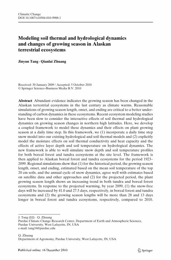
We apply both the coupled and uncoupled versions of the modeling frameworkand the parameterizations of tundra and boreal forest ecosystems to Alaska ata 0.2◦ × 0.2◦ (longitude by latitude) spatial resolution for the period 1923–2099(Fig. 1). The vegetation map is re-aggregated from the 0.05◦ × 0.05◦ resolutionMODIS L3 land cover type map with the international Geosphere Biosphere Pro-gramme (IGBP) classification for year 2004 (https://lpdaac.usgs.gov/lpdaac/products/modis_products_table/land_cover/yearly_l3_global_0_05deg_cmg/mcd12c1). We re-classify the forest vegetation types as boreal forest and other types including shrubtundra, savannas, and grasslands as generic tundra. The spatially-explicit dailyclimate data are from the Vegetation Ecosystem Modeling and Analysis Project(Kittel et al. 2000), which was created based on the historical climate (1922–1996)and the future HadCM2 scenario (1997–2099). The soil texture and elevation arefrom our previous studies (Zhuang et al. 2007). We simulate the top 20 cm averagesoil temperature and the daily snow depths. The onset of the growing season is thendefined by the date, starting from which in 10 consecutive days, the top 20 cm average

Fig. 1 Distribution of tundraand boreal forest ecosystemsin Alaska for the regionalapplication in this study,derived from the MODIS L3land cover type map for 2004(see text for details)

Climatic Change

soil temperature is greater than 2◦C; and the ending of growing season in defined bythe date, before which, in 10 consecutive days, the top 20 cm average soil temperatureis greater than 2◦C. This definition should be more robust than the one defined usingdaily air temperature (Sharratt 1992), as our simulations indicate there are chanceseven when the air temperature is above zero, the top layer of a soil column is still notsufficiently thawed. We examine changes of soil thermal regime and growing seasonthrough analyses of their absolute values and anomalies at different temporal andspatial scales. The output in year 1922 is discarded in the analysis of the regionalsimulation because of our model configuration.

3 Results and discussion

3.1 Site-level snow dynamics

The revised modeling framework performs well at the NSA-OBS site in simulat-ing snow depth dynamics (Fig. 2).We use 500-day data to calibrate snow modelparameters (Table 1). The comparison between the simulated and observed snowthickness has a root mean square error (RMSE) 6.02 cm, coefficient of determinationR2 = 0.90 of the linear regression y = 0.91x + 0.66 (p < 0.0001), with x being thesimulation and y being the observations. For the tundra site, we use a relativelylonger time period (4-year data) in calibration. The resulting overall agreement of thesimulated snow depth against the observations is of RMSE 11.47 cm, and R2 = 0.92of the linear regression y = 0.85x + 1.03 (p < 0.0001). Overall, the model capturesthe daily snow dynamics reasonably well.

3.2 Site-level soil thermal dynamics

For the NSA-OBS site, the simulated soil temperatures at different depths agreewell with the measurements from the top soil layer to deeper soil layers (Fig. 3). The

1994 1996 1998 2000 2002 2004 20060

50

100

150

Sno

w D

epth

(cm

)

a ObservationValidationCalibration

2000 2002 2004 2006

b

Fig. 2 Comparison of simulated snow depths versus observations. a NSA-OBS site: in calibration pe-riod y = 0.970x − 0.09 (cm), with y being the observation and x the simulation, the root mean squareerror (RMSE) is 3.56(cm) and R2 = 0.96 (p < 0.0001); in validation period y = 0.903x + 0.75 (cm),RMSE = 6.2 (cm) and R2 = 0.90 (p < 0.0001). b Tundra site: in calibration period, y = 0.913x + 1.40(cm), RMSE = 8.30 (cm), R2 = 0.94 (p < 0.0001); in validation period y = 0.816x + 0.17 (cm),RMSE = 14.4 (cm), R2 = 0.92 (p < 0.0001)

Climatic Change

–20

0

20

o C(a1) 5cm

– 20

0

20(b1) 10cm

o C

– 20

0

20

o C

(c1) 20cm

– 20

0

20(d1) 50cm

o C

1994 1996 1998 2000 2002 2004 2006

– 20

0

20

o C

(e1) 100cm

Observation

Calibration

Validation

(a2) 5cm

(b2) 10cm

(c2) 20cm

(d2) 50cm

1994 1996 1998 2000 2002 2004 2006

(e2) 100cm

Fig. 3 Comparison between the simulated soil temperature and observations at NSA-OBS site

coupled simulation performs slightly better than the uncoupled simulation in deepsoil layers (Table 2). However, as it goes deeper, the agreement becomes worse.The greater discrepancies between simulations and observations at deeper layers aremainly due to two reasons. First, in the current algorithm, only two phase planes are

Climatic Change

Tab

le2

Com

pari

son

ofth

em

odel

sim

ulat

ions

agai

nstt

hem

easu

rem

ents

inth

esi

te-l

evel

stud

y

Dep

ths

NSA

-OB

ST

undr

a

Cou

pled

Unc

oupl

edC

oupl

edU

ncou

pled

Slop

eIn

t.R

2R

MSE

Slop

eIn

t.R

2R

MSE

Slop

eIn

t.R

2R

MSE

Slop

eIn

t.R

2R

MSE

5cm

0.92

1.50

0.83

4.4

0.82

2.4

0.90

4.0

0.85

0.82

0.88

2.6

0.86

0.02

0.88

2.3

1.01

0.92

0.83

4.0

1.10

−0.5

60.

913.

10.

881.

130.

823.

10.

880.

030.

813.

110

cm0.

980.

420.

833.

90.

771.

350.

883.

40.

860.

920.

832.

70.

75−0

.00

0.84

2.4

1.29

−0.5

40.

745.

11.

29−0

.89

0.84

3.9

0.93

1.28

0.79

3.1

0.80

0.09

0.78

2.7

20cm

1.07

0.03

0.81

3.9

0.68

0.97

0.80

3.5

0.81

0.85

0.77

2.7

0.62

−0.2

00.

742.

80.

970.

420.

784.

00.

900.

340.

823.

30.

901.

180.

723.

10.

69−0

.05

0.70

2.8

50cm

0.83

−0.3

00.

811.

21.

060.

450.

781.

50.

620.

350.

622.

90.

51−0

.16

0.61

2.8

0.60

−0.6

10.

261.

90.

30−1

.17

0.03

3.4

0.71

0.54

0.58

2.8

0.58

−0.0

90.

582.

610

0cm

0.23

0.06

0.15

0.56

0.47

0.24

0.16

0.75

0.42

0.45

0.35

3.1

0.30

0.07

0.25

3.2

0.57

−0.3

50.

211.

650.

730.

120.

170.

210.

450.

440.

232.

80.

420.

190.

282.

515

0cm

NA

NA

NA

NA

NA

NA

NA

NA

0.42

0.34

0.38

2.9

0.34

0.07

0.34

2.9

NA

NA

NA

NA

NA

NA

NA

NA

0.48

0.37

0.43

2.7

0.43

0.10

0.43

2.5

Uni

tsof

slop

e,in

terc

ept

(Int

.),a

ndro

otm

ean

squa

reer

ror

(RM

SE)

are

N/A

,◦C

and

◦ C.F

orea

chdi

ffer

ent

dept

h,th

ese

cond

row

isst

atis

tics

inth

eva

lidat

ion

peri

od

Climatic Change

accounted explicitly in solving the heat conduction equation (Goodrich 1976).Whena new phase plane is initiated at the surface in accordance with a change of freeze–thaw status, the temperature at the computational nodes (i.e. depth steps) betweenthe new phase plane and the previous top phase plane is set to 0◦C. At the nextmodel time step, the middle phase plane is ignored and only the movements oftop and bottom phase planes are tracked. This treatment appears reasonable formaterials like water (see Goodrich 1976 and reference therein), but nevertheless itarbitrarily introduces or removes energy from the soil profile, resulting in solutionerrors. The second reason is that, we lack detailed soil moisture data to constrain thehydrological processes, and the soil profile of the black spruce forest ecosystem isapproximated based on podzols (FAO-Unesco 1990). Thence there are chances thatthe soil moisture profile simulated deviates from the site data at a daily time step.The simulated evapotranspiration and the soil moisture in mineral layer generallyagree with the observed data (Figs. 4 and 5). However, the model underestimatessoil moisture in generic organic layer in year 1996 and overestimates in 1997 incomparison with the observations (Fig. 5). It is likely due to the lack of detailedinformation of the soil profile and sufficient soil moisture data for calibration, as weexplained before.

For the tundra site, similar to the boreal forest site, the coupled simulationperforms slightly better than the uncoupled simulation and greater discrepanciesbetween the simulation and observation are found in deeper soil layers (Fig. 6,Table 2). The reasons for the deteriorating performance at deeper layers are thesame as that at the boreal forest site. Also, when the linear fitting of the simulationagainst the measurements is conducted, the coupled version shows a slightly betterperformance as its slope is closer to one, and a greater R2 value of the fitting. Forinstance, at depth 1.5 m, the coupled simulation has its linear fitting slope 0.42/0.48(calibration/validation), R2 value 0.38/0.43, and the uncoupled simulation has theslope 0.34/0.43, R2 value 0.34/0.43.

Fig. 4 Comparison of thesimulated evapotranspirationagainst measurement for theNSA-OBS site. In calibrationperiod y = 0.796x + 5.10(mm), RMSE = 7.51 (mm),R2 = 0.91 (p < 0.0001); invalidation periody = 0.796x + 6.63 (mm),RMSE = 8.89 (mm),R2 = 0.86 (p < 0.0001)

1994 1996 1998 2000 2002 2004 20060

20

40

60

80

100

H2O

(mm

)

Year

ObservationCalibrationValidation

Climatic Change

Fig. 5 Comparison betweenthe simulated soil moistureand measurement for the forthe NSA-OBS site. Thetemporally sporadic daily orhourly measurements ofvolumetric soil moisture forthe humic organic and mineralsoil layers are aggregated tomonthly resolution forcomparison. The humicorganic soil moisture wasestimated as the mean of allsoil moisture measurementsshallower than 45 cm, whilethe mineral soil moisture wasestimated as the mean of allsoil moisture measurementsdeeper than 45 cm andshallower than 105 cm

0

10

20

30

40

50

60

Vol

umet

ric s

oil m

oist

ure

(%)

a

May Jul Sep Nov Jan Mar May0

10

20

30

40V

olum

etric

soi

l moi

stur

e (%

)

1996 1997

b

SimulationMeasurement

Through site-level studies, we obtained two sets of parameters for boreal forestand tundra ecosystems (Tables 3 and 4), which will be used for our regionalextrapolation.

3.3 Historical regional soil thermal, hydrological, and growing season dynamics

3.3.1 Historical soil thermal dynamics

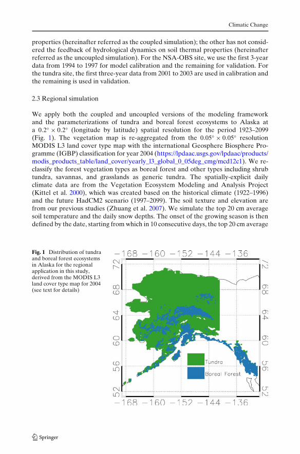
Soil temperature shows a significant increase over most of the study domain inresponse to the warming (Fig. 7). The decadal mean seasonal anomalies of the top20 cm average soil temperature are computed for the spring (March 1st to May 31st)and autumn (September 1st to November 30th) in the 1930s, 1980s, 2030s and 2080s.The annual anomaly for a certain season in a given year is defined as the differencebetween the mean soil temperature for that season during the year and the mean ofthe mean soil temperature for that season during the period 1923–2099. The decadalmean seasonal anomaly is then calculated as the average of the annual anomalies ofthe season over the given decade. The computation is done separately for both thecoupled and uncoupled simulations. The autumn top 20 cm mean soil temperaturein the 1980s is higher than in the 1930s in most areas, in response to the increasingof air temperature, after recovering from the cold period between the 1940s and the1970s. In the northern polar region, the autumn top 20 cm mean soil temperaturein the 1980s is however lower than that in the 1930s, in accordance with the coolerautumn in the 1980s compared to the 1930s.

The soil temperature varies at different scales, and the warming trend is notvery significant. In most boreal forest region (spatial anomaly not shown), the soiltemperature decreases in the 1940s compared to that in the 1930s in both spring

Climatic Change

–20

0

20

o C

(a1) 5cm

– 20

0

20 (b1) 20cm

o C

– 20

0

20

o C

(c1) 50cm

– 20

0

20 (d1) 100cm

o C

2001 2002 2003 2004 2005 2006

– 20

0

20

o C

(e1) 150cm

Observation

Calibration

Validation

(a2) 5cm

(b2) 20cm

(c2) 50cm

(d2) 100cm

2001 2002 2003 2004 2005 2006

(e2) 150cm

Fig. 6 Comparison between the simulated soil temperature and observations at tundra site

and autumn seasons. This decrease continues till the 1960s, and then the autumntemperature begins to increase in the 1970s, while the spring temperature stilldecreases. In the 1980s, the spring temperature increases almost over the wholeregion compared to the 1970s, and the autumn temperature increases in a smaller

Climatic Change

Table 3 Parameters for the tundra and boreal forest ecosystems used by coupled simulation inregional application

Parameter Tundra Boreal Forest Unit Source

First layer organic matter content 90.0 71.0 % CalibrationFirst layer bulk density 113.6 82.8 kg m−3 CalibrationFirst layer saturated matric potential −109.8 −126.8 mm CalibrationFirst layer saturated hydraulic conductivity 0.15 0.12 mm−1 CalibrationFirst layer Clap and Hornberg constant 4.0 1.0 None Beringer et al.

(2001)Second layer organic matter content 23.0 75.0 % CalibrationSecond layer bulk density 883.6 997.7 kg m−3 CalibrationThird layer organic matter content 5.0 27.0 % CalibrationThird layer bulk density 1043.8 1351.5 kg m−3 CalibrationFourth layer organic matter content 8.0 4.0 % CalibrationFourth layer bulk density 1197.0 1108.9 kg m−3 CalibrationFifth layer organic matter content 6.0 2.0 % CalibrationFifth layer bulk density 1123.8 1829.4 kg m−3 CalibrationSixth layer organic matter content 6.0 5.0 % CalibrationSixth layer bulk density 1167.0 1287.9 kg m−3 Calibration

region in interior Alaska. Soil temperature in tundra ecosystems even decrease inautumn season. During the 1990s, both spring and autumn soil temperature increaseat a greater rate than before.

Table 4 Parameters for the tundra and boreal forest ecosystems used by uncoupled simulation inregional application

Parameter Tundra Boreal Forest Unit Source

First layer organic matter content 85.0 94.0 % CalibrationFirst layer bulk density 135.9 133.6 kg m−3 CalibrationFirst layer volumetric water content 0.12 0.15 m−3 water m−3 soil CalibrationSecond layer organic matter content 23.0 74.0 % CalibrationSecond layer bulk density 855.3 979.1 kg m−3 CalibrationSecond layer volumetric water content 0.54 0.36 m−3 water m−3 soil CalibrationThird layer organic matter content 9.0 17.0 % CalibrationThird layer bulk density 1612.9 1040.7 kg m−3 CalibrationThird layer volumetric water content 0.34 0.08 m−3 water m−3 soil CalibrationFourth layer organic matter content 4.0 4.0 % CalibrationFourth layer bulk density 1486.0 1148.8 kg m−3 CalibrationFourth layer volumetric water content 0.42 0.44 m−3 water m−3 soil CalibrationFifth layer organic matter content 5.0 4.0 % CalibrationFifth layer bulk density 1795.3 1183.7 kg m−3 CalibrationFifth layer volumetric water content 0.38 0.37 m−3 water m−3 soil CalibrationSixth layer organic matter content 7.0 4.0 % CalibrationSixth layer bulk density 1782.3 1462.0 kg m−3 CalibrationSixth layer volumetric water content 0.34 0.34 m−3 water m−3 soil Calibration

The soil hydraulic properties of the top layer are assumed same as for the coupled simulation

Climatic Change

Fig. 7 Decadal anomalies of seasonal mean soil temperature of the top 20 cm soil for the fourdecades, separated by every 50 years. The left two columns are from the coupled simulation, theright two columns are from the uncoupled simulation

3.3.2 Historical hydrological dynamics

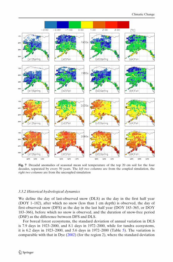
We define the day of last-observed snow (DLS) as the day in the first half year(DOY 1–182), after which no snow (less than 1 cm depth) is observed, the day offirst-observed snow (DFS) as the day in the last half year (DOY 183–365, or DOY183–366), before which no snow is observed, and the duration of snow-free period(DSF) as the difference between DFS and DLS.

For boreal forest ecosystems, the standard deviation of annual variation in DLSis 7.9 days in 1923–2000, and 8.1 days in 1972–2000, while for tundra ecosystems,it is 6.2 days in 1923–2000, and 5.6 days in 1972–2000 (Table 5). The variation iscomparable with that in Dye (2002) (for the region 2), where the standard deviation

Climatic Change

Tab

le5

Tre

nds

for

snow

-cov

ercy

cle

vari

able

s

Ana

lysi

s/re

gion

Tre

ndSt

anda

rdde

viat

ion

1923

–200

019

72–2

000

2010

–209

919

23–2

000

1972

–200

020

10–2

099

Bor

ealF

ores

tD

ayof

last

obse

rved

snow

−0.9

(0.0

3)−4

.7(0

.01)

−2.7

(<0.

01)

7.9

8.1

10.4

Day

offi

rsto

bser

ved

snow

−0.6

(0.0

3)−1

.1(0

.38)

2.0

(<0.

01)

5.8

5.5

8.4

Len

gth

ofsn

ow-f

ree

peri

od0.

2(0

.70)

3.6

(0.1

4)4.

7(<

0.01

)10

.710

.916

.4T

undr

aD

ayof

last

obse

rved

snow

−0.2

(0.4

8)−2

.0(0

.11)

−1.6

(<0.

01)

6.2

5.6

6.3

Day

offi

rsto

bser

ved

snow

−0.2

(0.4

2)−0

.2(0

.87)

1.3

(<0.

01)

4.8

5.2

5.8

Len

gth

ofsn

ow-f

ree

peri

od0.

1(0

.96)

1.8

(0.3

4)2.

9(<

0.01

)8.

78.

410

.2

Uni

tsfo

rtr

ends

and

stan

dard

devi

atio

nar

e,re

spec

tive

ly,d

ays

per

deca

dean

dda

ys.T

hose

inbr

aces

are

pva

lues

ofth

elin

ear

fitt

ing

Climatic Change

of the week of last-observed snow cover (WLS) as he defined for the weekly, visible-band satellite observations of Northern Hemisphere snow-cover from NOAA in1972–2000, is around 1.0 weeks (around 7.0 days). The standard deviations of theDFS and DSF of our simulated data are similar to Dye (2002)’s study. The weekof first-observed snow cover (WFS) and DSF are 0.7 weeks (around 5.6 days) and1.2 weeks (around 8.4 days), respectively, in his study. The DLS in boreal forestecosystems and tundra ecosystems show an earlier shift of 4.7 and 2.0 days perdecade, respectively. The magnitude of earlier WLS shift in Dye (2002) is 5.0 daysper decade, which is greater. A possible reason is that his data are at a weeklytime step, while our simulation is at a daily time step. Also, our simulation coversa smaller region than that of the region 2 in Dye (2002). For the trend in DFS, theboreal forest ecosystems and tundra ecosystems show a magnitude of −1.1 days perdecade (p = 0.38) and −0.2 days per decade (p = 0.87), respectively, in 1972–2000,both of which are smaller than 0.4 days per decade in Dye (2002). The trend of oursimulated DSF in boreal forest ecosystems and tundra ecosystems in 1972–2000 is3.6 and 1.8 days per decade, still smaller than 5.3 days per decade estimated by Dye(2002). Stone et al. (2002) found the snow-melt date in northern Alaska has advancedby 8 days or so, since the mid-1960s. Our simulations show, in areas north of 69◦N,that the DLS advanced 4.0 ± 2 days in the same time period. With the time series ofmelt dates at the Barrow (BRW) National Weather Service and NOAA/CMBDL-BRW radiometric observations and proxy estimates determined from temperaturerecords, Stone et al. (2002) stated that the melt days have advanced by 7.7 ± 4.4 daysduring 1940–2000. We estimate the DLS in north of 69◦N has decreased 8.7 ± 1.9 daysin the same time period, which is close to their estimates. Tedesco et al. (2009)estimated, based on space-borne passive microwave data, that the snow free dayshave lengthened around 5 days per decade, during the period 1979–2008 for the panarctic region. Our study indicates a trend of 1.55 days per decade (p = 0.37) in borealforest ecosystems and −0.66 days per decade (p = 0.73) in the tundra ecosystems,which are different from Tedesco et al. (2009). This difference is mainly caused bythe uncertainty in the climate data we have used, which was created before 2000(Kittel et al. 2000).

The coupled and uncoupled simulations of soil moisture are very different atvarious scales (Fig. 8). Specifically, the spring volumetric soil moisture of the 1980s inthe coupled simulation is relatively lower (drier) than that in the 1930s, while in theuncoupled simulation, the 1980s anomaly is higher (wetter) in most of the northernpolar regions than that in the 1930s. The precipitation was generally greater in springand summer in the 1980s than in the 1930s, and was lower in autumn in the 1980s thanin the 1970s. The difference in modeled soil moisture is due to the impedance effectof the frozen water in the coupled simulation. When ice is present, the hydraulicconductivity is significantly reduced, and the amount of liquid water available forinfiltration after runoff in the soil column is much less than that in the case if frozenwater is otherwise neglected (Lundin 1990; Oleson et al. 2004). Therefore, in thehistorical period, the coupled simulation shows a different response to the variationof precipitation and evapotranspiration from the uncoupled simulation does in theregion (Figs. 8 and 9). In the autumn season, the coupled simulation of soil moistureagain shows a stronger positive response to the decrease of precipitation. Due to thelack of thermal impact on liquid water transport, the area-weighted moisture in theuncoupled simulation is lower than that in the coupled simulation.

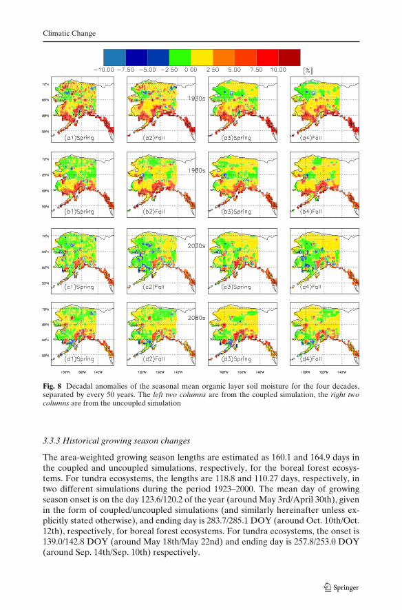
Climatic Change

Fig. 8 Decadal anomalies of the seasonal mean organic layer soil moisture for the four decades,separated by every 50 years. The left two columns are from the coupled simulation, the right twocolumns are from the uncoupled simulation

3.3.3 Historical growing season changes

The area-weighted growing season lengths are estimated as 160.1 and 164.9 days inthe coupled and uncoupled simulations, respectively, for the boreal forest ecosys-tems. For tundra ecosystems, the lengths are 118.8 and 110.27 days, respectively, intwo different simulations during the period 1923–2000. The mean day of growingseason onset is on the day 123.6/120.2 of the year (around May 3rd/April 30th), givenin the form of coupled/uncoupled simulations (and similarly hereinafter unless ex-plicitly stated otherwise), and ending day is 283.7/285.1 DOY (around Oct. 10th/Oct.12th), respectively, for boreal forest ecosystems. For tundra ecosystems, the onset is139.0/142.8 DOY (around May 18th/May 22nd) and ending day is 257.8/253.0 DOY(around Sep. 14th/Sep. 10th) respectively.

Climatic Change

Fig. 9 Decadal area-averagedspring volumetric soil moistureof the organic layer. a Spring;b Autumn. The error barsshow the standard deviationduring the given decade

10

15

20

25

30

35

40

%

a

1920 1940 1960 1980 2000 2020 2040 2060 2080 21000

10

20

30

40

50

%

bBoreal Forest: coupled

Boreal Forest: uncoupled

Tundra: coupled

Tundra: uncoupled

There is a strong inter-annual variability in the day of onset, day of endingand lengths of the growing seasons in our study period. Specifically, the coupledsimulation shows that, for boreal forest ecosystems, in 1923, the growing seasonlength is about 172 days; in 1924, it becomes 156 days; and in 1925, it is nearly168 days. Similar behavior is also found for tundra ecosystems. The mean amplitudes(characterized by standard deviation) of inter-annual variation of the growing seasonlengths for boreal forest and tundra ecosystems are about 8.3/6.4 and 6.4/6.1 days,respectively, in the period 1923–2000. Analysis of variance shows such an inter-annual variability is almost equally contributed by the variation in the day of growingseason onset and the day of growing season ending.

At a decadal scale, the growing season lengths in both boreal forest and tundraecosystems experience a slight decrease in the 1940s and the 1950s, then an increasein the 1960s (Fig. 10). The 1960s’ increasing continues to the 1990s. The changes ofthe growing season length can be attributed to changes in both the day of onset andthe day of ending. An early day of growing season onset is not simply associated witha late day of ending. For instance, in the 1990s, when the mean growing season lengthis longer than that in the 1980s for boreal forest ecosystems, the mean day of onset inthe 1990s is earlier than that in the 1980s, and the mean day of ending in the 1990s islater than in the 1980s. However, in the 1980s, when mean growing season length inboreal forest ecosystems is longer than that in the 1970s, both the mean day of onsetand the mean day of ending are earlier than those in the 1970s.

At a longer temporal scale, the changes of growing season showed a greatervariability in the historical period (Fig. 11, Table 6). During 1923–1950, the growingseason lengths in tundra ecosystems in the northern polar region show a significantnegative trend of change in both coupled and uncoupled simulations. The east andsouthwest Alaska show a lengthened growing season in the same period. When thearea-averaged statistics were analyzed, both tundra and boreal forest ecosystemsshow the growing season lengths were shortened in 1923–1950 because of the delayedonset and advanced growing season ending. From 1950 to 2000, the area-averagedgrowing season length in boreal forest ecosystems increased 1.6 days per decade

Climatic Change

100

150

200

250D

ays

a

80

100

120

140

160

Day

of Y

ear

b

1920 1940 1960 1980 2000 2020 2040 2060 2080 2100240

260

280

300

320

Day

of Y

ear

c

Boreal Forest: coupled

Boreal Forest: uncoupled

Tundra: coupled

Tundra: uncoupled

Fig. 10 a Decadal area-averaged growing season length. b Decadal area-averaged day of growingseason onset. c Decadal area-averaged day of growing season ending. The variables are defined bydays with top 20 cm soil temperature greater than 2◦C, for the period 1923–2099. The error bars showthe standard deviation during the given decade. See text for statistics of trend

(p = 0.05), and 1.4 days per decade (p = 0.02) in tundra ecosystems in the coupledsimulation. The day of onset in boreal forest ecosystems is earlier by 1.5 days perdecade (p < 0.01) and by 0.9 days per decade (p = 0.05) in tundra ecosystems; theday of ending in boreal forest ecosystems is delayed by 0.1 days per decade (p = 0.81)and by 0.5 days per decade (p = 0.15) in tundra ecosystems.

Comparison between our estimates of annual growing season cycle in 1981–1990to that derived from satellite NDVI for the region north of 45◦N (Myneni et al.1997) shows, that the day of onset was significantly shifted to an earlier DOY inboth the boreal forest and the tundra ecosystems and the shift in tundra ecosystem isrelatively smaller (Fig. 12). Similar to Myneni et al. (1997), we use seven successivetemperature thresholds from 0.0◦C (with an incremental 0.5◦C) to 3.0◦C to determinegrowing seasons and their associated variations. The area-averaged growing seasononset is estimated for the coupled simulation with an advance of 13.7 ± 1.9 days(13.4 ± 2.5 days in the uncoupled simulation) for boreal forest ecosystems, and2.2 ± 0.5 days (3.4 ± 1.2 days in the uncoupled simulation) for tundra ecosystemsin the 10-year period 1981–1990 (Fig. 12). These estimates are similar to the estimateof 8 ± 3 days by Myneni et al. (1997) for the same period. For the growing season

Climatic Change

Fig. 11 Long-term trend in growing season lengths for the different time periods. The left twocolumns are for the coupled simulations, the right two columns are for the uncoupled simulations. a1,a3, b1, b3, c1, c3, d1 and d3 are the inferred trend. The rest are p values of the trend

ending, we estimate a delay of 3.9 ± 1.7 days (7.2 ± 3.4 days in the uncoupledsimulation) and 2.5 ± 1.7 days (2.3 ± 1.4 days in the uncoupled simulation), whereasMyneni et al. (1997) estimated a prolongation of 4 ± 2 days between 1982–3 and1989–90. We estimate that in boreal forest ecosystems the growing season length is9.7 ± 2.8 days (6.2 ± 5.7 days in the uncoupled simulation) longer, and in tundraecosystems 4.7 ± 2.1 days (5.7 ± 1.6 days in the uncoupled simulation) longer, whichare comparable to the estimates of 12 ± 4 days longer in north of 45◦N in Myneniet al. (1997) for the period 1981–1990.

Some recent studies have extended the analysis of greening and browning to themost recent periods using satellite data (Jia et al. 2003; Goetz et al. 2005; Bunnet al. 2007; Verbyla 2008). In Jia et al. (2003) and Verbyla (2008), they all foundthe peak NDVI increased since the 1980s, with greater increasing in the tundraecosystems. A decreasing trend was found in boreal forest ecosystems since the 1980s

Climatic Change

Tab

le6

Tre

ndst

atic

sof

the

grow

ing

seas

onon

set,

endi

ngan

dle

ngth

s

Tem

pora

lper

iod

1923

–195

019

51–2

000

2010

–209

9

Bor

ealF

ores

tT

undr

aB

orea

lFor

est

Tun

dra

Bor

ealF

ores

tT

undr

a

Cou

pled

Are

aw

eigh

ted

onse

t0.

4(0

.71)

0.4

(0.6

6)−1

.5(<

0.01

)−0

.9(0

.05)

−2.1

(<0.

01)

−0.9

(<0.

01)

Are

aw

eigh

ted

endi

ng−1

.7(0

.18)

−0.9

(0.3

1)0.

1(0

.81)

0.5

(0.1

5)1.

7(<

0.01

)1.

1(<

0.01

)G

row

ing

seas

onle

ngth

−2.1

(0.3

0)−1

.3(0

.39)

1.6

(0.0

5)1.

4(0

.02)

3.8

(<0.

01)

2.0

(<0.

01)

Unc

oupl

edA

rea

wei

ghte

don

set

0.9

(0.5

5)0.

5(0

.58)

−1.8

(<0.

01)

−0.7

(0.0

6)−2

.2(<

0.01

)−0

.9(<

0.01

)A

rea

wei

ghte

den

ding

−1.5

(0.2

0)−1

.1(0

.23)

−0.1

(0.9

3)0.

6(0

.14)

1.6

(<0.

01)

1.2

(<0.

01)

Gro

win

gse

ason

leng

th−2

.4(0

.29)

−1.5

(0.3

0)1.

7(0

.04)

1.3

(0.0

3)3.

8(<

0.01

)2.

1(<

0.01

)

Uni

tsfo

rtr

ends

are

days

per

deca

de.T

hose

inbr

aces

are

pva

lues

ofth

elin

ear

fitt

ing

Climatic Change

100 110 120 1300

2

4

6

o C

(a1)

290 300 310

(a2)

120 130 140 150

(b1)

260 270 280

(b2)

0 40 80 120 160 200 240 280 320 36030

20

10

0

10

20o C

(a) Boreal Forest Coupled

0 40 80 120 160 200 240 280 320 360

(b) Tundra

1981&82 mean1983&84 mean1985&86 mean1987&88 mean1989&90 mean

100 110 120 1300

2

4

6

o C

Day of year

(c1)

290 300 310Day of year

(c2)

120 130 140 150Day of year

(d1)

260 270 280Day of year

(d2)

0 40 80 120 160 200 240 280 320 360 30

20

10

0

10

20

o C

(c) Boreal Forest

0 40 80 120 160 200 240 280 320 360

(d) Tundra

1981&82 mean1983&84 mean1985&86 mean1987&88 mean1989&90 mean

Fig. 12 Area-averaged top 20 cm soil temperature for the 1980s: (a1) and (a2), (b1) and (b2), (c1)and (c2), (d1) and (d2) are, respectively, blow-up plots for panel (a), (b), (c) and (d)

to 2000, even though with an increasing summer warmth index. The decreasing trendwas explained as a result of a number of factors, including drought stress, insectand disease infestations. In our study, we found trends of increasing in growingseason length are mixed with trends of decreasing throughout the Alaska (Fig. 11).Also, the soil moisture in the organic layer in the boreal forest ecosystems wasfound decreased both in the coupled and uncoupled simulations in the springs andautumns of this period (e.g. Fig. 9). This is in agreement with the finding of waterstress in their studies. Therefore, given the climate data used in simulation, weare doing a reasonable hindcast of the soil thermal and hydrological dynamics, as

Climatic Change

well as growing season statistics, for Alaskan terrestrial ecosystems in the historicalperiod.

3.4 Future soil thermal and hydrological dynamics and growing season changes

Abundant inter-annual variability exists in the projected soil temperature, and thetrend of soil warming is found much more significant than that in the historicalperiod. The warming trend is found stronger in the tundra ecosystems (Fig. 7) in thenorthern polar region. Generally, the simulated warming in the soil thermal regimeis more substantial in the coupled simulation than in the uncoupled simulation dueto the modulation effects of soil moisture on soil temperature. Since the uncoupledsimulation used the fixed soil moisture for each soil layer, the moisture in the secondlayer appears higher than that simulated in the coupled simulation. Thence the soilcolumn in the uncoupled simulation is less sensitive to the warming because of itshigher heat capacity in presence of more water.

The spring soil moisture is projected to decrease in both the coupled and un-coupled simulations because of the projected increasing in evapotranspiration (datanot shown). However, as the precipitation is also projected to increase, the 2030s’mean autumn soil moisture appears higher than the 1980s’ in tundra areas andthe increase is found stronger in the uncoupled simulation. This is because, in thecoupled simulation, the ice in tundra soils needs time to thaw in order to changethe hydraulic conductivities. As warming continues, the hydraulic properties in thecoupled simulation become similar to that in the uncoupled simulation, and theirsimulations of soil moisture become more similar (Fig. 9).

For the projected snow dynamics, the DSF in both tundra and boreal forestecosystems increases significantly due to an earlier DLS and later DFS. From 2010to 2099, the projected DLS approaches by 29.1 days in boreal forest ecosystems andby 23.4 days in tundra ecosystems. The projected DFS comes earlier by 12.0 days inboreal forest ecosystems and by 4.0 days in tundra ecosystems. Such changes in theDLS and DFS result in a growing season lengthening by more than 3 weeks longerby the end of the 21st century in comparison with 2010.

The mean area-weighted growing season length in 2010–2099 is 181.8/187.9 daysfor boreal forest ecosystems and 132.2/124.3 days for tundra ecosystems. The meanday of growing season onset and ending are 110.9/105.5 DOY, and 292.7/293.4 DOYin boreal forest ecosystems, and 133.3/137.6 DOY and 265.4/261.9 DOY in tundraecosystems. Both boreal forest and tundra ecosystems show a significant increasingtrend in the growing season length, due to an earlier onset and a later ending. Therate of growing season length increasing in boreal forest ecosystems is as much as 3.8and 2.0 days per decade in tundra ecosystems.

We tested the sensitivity of the projection to the climate forcing by repeating thesimulations by perturbing the original air temperature data ±1◦C and precipitationdata ±10%. For the boreal forest ecosystem, the 1◦C increase (decrease) changedthe trend of DSF by 0.1 (−0.03) days per decade. The trend of DFS is more sensitiveto warming than to cooling, while the opposite is for that of the DLS, but theabsolute magnitude of sensitivity is less than 0.1 days per decade. For the tundraecosystems, the 1◦C increase (decrease) changed the trend of DSF by 0.02 (0.01)days per decade. Similarly, the DFS is more sensitive to warming than to cooling,while the opposite is for the DLS, with an absolute magnitude less than 0.1 days

Climatic Change

per decade. For both the boreal forest and tundra ecosystems, the 10% increasein precipitation hardly changed the trend statistics of DLS, DFS and DSF, whilethe 10% decrease in precipitation changed the trend statistics of DLS, DFS andDSF by an absolute magnitude less than 0.05 days per decade. For the projectionof growing season, it is found a 1◦C increase (decrease) in air temperature changedthe trend of growing season length by 0.04 (−0.11) days per decade for boreal forestecosystem, and by −0.09 (0.11) days per decade for tundra ecosystem. The increasein the positive trend of growing season length in the tundra ecosystem occurred for1◦C decrease rather than for 1◦C increase, is manifested as a sharper delay in thegrowing season ending. However, the length of growing season in the simulation with−1◦C perturbation is shorter, and that with 1◦C perturbation is longer. The sensitivitystrengths are quite similar in both the coupled and uncoupled simulations. Similaras for the statistics of snow, the change of precipitation with ±10% did not changethe statistics much (less than 0.1 days per decade in absolute magnitude) for boththe boreal forest and tundra ecosystems, though the sensitivity is slightly greater inboreal forest ecosystems. Therefore, we concluded that our projection is robust withrecognition of uncertainty of the forcing data used in this study.

4 Conclusions and future studies

In this study, we investigate the change of growing season through modeling soilthermal and hydrological dynamics of Alaskan tundra and boreal forest ecosystemsin 1923–2099. We first revise an existing framework of soil thermal and hydrologicalmodels for the cold region by explicitly considering the interactions between soilthermal and hydrological dynamics. Our simulations suggest that the coupled versionof the modeling framework performs better than the uncoupled version. The revisedmodeling framework well simulates soil thermal and hydrological dynamics and thechanges of growing season. The estimated regional snow dynamics and growingseason changes are comparable with satellite-based estimates for both tundra andboreal forest ecosystems. Our future research will incorporate the effects of fire dis-turbances (1) on changes of organic matter content of the top-soil layers (Lawrenceet al. 2008), (2) on soil thermal conductivity and heat capacity (Zhuang et al. 2002)and (3) on hydrological dynamics in the modeling framework. We will also considerthe effects of vegetation changes on snow dynamics (Arsenault and Payette 1992),thus on both soil hydrological and thermal dynamics. The new modeling frameworkwill be further coupled with our existing biogeochemistry model, the TerrestrialEcosystem Model (TEM; Zhuang et al. 2003, 2004, 2007) to study carbon dynamicsin northern high latitudes.

Acknowledgements We thank Dr. Steve Wofsy and his group at Harvard University to makethe soil temperature and latent heat flux measurements at the black spruce site available and theEcosystem Center of Marine Biological Laboratory at Woods Hole to make the soil temperatureand meteorological data at the tundra site available for this study. J. Tang is supported with thePurdue Climate Change Research Center Graduate Fellowship and NASA Earth System ScienceFellowship. The research is also supported by the National Science Foundation with projectsof ARC-0554811 and EAR-0630319. The computational support is from Rosen Center for HighPerformance Computing at Purdue University. Comments from Dr. Nigel Roulet and an anonymousreviewer and the Editor made great improvements on an earlier draft of this paper.

Climatic Change

Appendix 1: Snow dynamics

We modify a snow model from Karvonen (2003) to compute the snow depth anddensity for our revised modeling framework. Given the amount of precipitation Pc

(mm day−1) and the corresponding air temperature Ta (◦C), the amount of snowfalland rainfall is computed

fW =

⎧⎪⎪⎨

⎪⎪⎩

1.0Ta − Tsnow

Train − Tsnow0.0

,

,

,

Ta ≥ Train

Tsnow < Ta < Train

Ta ≤ Tsnow

Prain = fWCW Pc

Psnow = (1 − fW)CS Pc

(4)

When daily air temperature Ta is below Tsnow (◦C), the precipitation falls as snow.When Ta is higher than Train (◦C), the precipitation will fall as rainfall. CW and CS

are correction factors for water and snow, whose values are, respectively, set to 1.06and 1.32 (Karvonen 2003).

In presence of vegetation, part of the precipitation will be intercepted by plants,and the remaining falls to the ground. We following the work of Coughlan andRunning (1997) to compute the snow interception by plants, such that

PSI = LAIIS,MAX

2SIi = min(PSI − SAi, Psnow,i) (5)

where SIi (mm) is the snow intercepted in day i, and SAi (mm) is the snow remains onthe plants in day i after accounting for snow sublimation in the previous day. IS,MAX

is the daily interception of snow per unit leaf area. The plant interception of rainfallis computed in a way similar to the snow interception, but the maximum interceptrate is computed using the formula in Helvey and Patric (1965).

After accounting for the plant interception, the through-fall of precipitation isadded to two pools, the accumulated snow XS (mm) and accumulated liquid waterXR (mm), on the ground, which are governed by the following equations

dXS

dt= Psnow,thru − Smelt + Srefreeze

dXR

dt= Prain,thru − Srefreeze − Outf low (6)

where Psnow,thru (mm day−1) and Prain,thru (mm day−1) are the through-fall of snowand rain to the ground.

The snowmelt Smelt (mm day−1) is computed based on a degree-day factor throughthe following equation

Smelt = KM(Ta − TB,M

)

KM = KMIN (1 + KCUM MCUM) , KM ≤ KMAX (7)

where KM is the degree-day factor (mm ◦C day−1), TB,M (◦C) is base temperature formelting, KMIN and KMAX are the minimum and maximum values for the degree-day

Climatic Change

factor. MCUM (mm) is the cumulative snowmelt during the winter/spring, and KCUM

(mm−1) is a parameter denoting the increase in degree-day factor given one mmchange in snow accumulation.

Snow is able to store a certain amount of liquid water until it becomes sufficiently“wet”, such that it reaches the maximum snow density. We model such process byintroducing a water retention capacity, such that

fCAP = fC,MAX (1 − CCUM MCUM) , fCAP ≥ fC,MIN

Sliq = fCAPSWE (8)

where Sliq (mm) is the amount of liquid water stored in the accumulated waterequivalent snow SWE (mm).

When temperature is low and there is liquid water stored in ground snowpack,refreezing process could occur to change liquid water into ice crystals, adding to theamount of accumulated snowpack. Such process is modeled through the followingequation

Srefreeze = KF(TB,F − Ta

)eF, Ta < TB,F

Srefreeze = 0 , Ta ≥ TB,F (9)

where TB,F is the base temperature for refreezing, KF (mm ◦C−1 day−1) is therefreezing parameter and eF is the exponent coefficient for refreezing.

The outflow in day i is computed as a residual of the total liquid water XR (mm)accumulated in day i (including new rainfall and snowmelt) after subtracting the totalamount of liquid water that can be held in the wet snow (Sliq). If otherwise the XR

is less than Sliq, no outflow is allowed. The outflow, if available, is used to computethe surface runoff and infiltration following our original formulations of the model(Zhuang et al. 2004). With the amount of accumulated snowpack, the snow densityand depth are computed as

ρS,i = (1 + ρPACK)ρS,i−1 DS,i−1 + ρNEW Psnow,i

DS,i−1 + Psnow,i

ρS,i ≤ ρMAX

DS,i = SW E,i

ρS,i(10)

where ρS,i−1 (kg dm−3) and DS,i−1 (mm) are snow density and snow depth of theprevious day, Psnow,thru,i is the amount of new snow through-fall in day i, ρNEW isdensity of new snow and ρPACK is a snow-packing parameter that accounts for theeffect of snow compaction. Further, it assumes the snow density is no greater thanρMAX.

Climatic Change

Appendix 2: Soil thermal properties

Following Balland and Arp (2005), the Kersten number is defined as, for unfrozensoils

Ke = θ0.5(1+Vom,s−αVsand,s−Vcf,s)sat

×[(

11 + exp(−βθsat)

)3

−(

1 − θsat

2

)3]1−Vom,s

(11)

and for frozen or partially frozen soils

Ke = θ1+Vom,ssat (12)

where the adjustable parameters α and β are assumed 0.24 and 18.3. Vom, Vsand,s andVcf,s are the volumetric fractions of organic matter, sand and coarse fragments withinthe soil solids. θsat is the degree of saturation computed with

θsat = Vwater + Vice

Vpores(13)

where Vpores = 1 − ρb/ρp with ρb being the bulk density of soil, and ρp the particledensity of the soil, given by

ρp = Wom/ρom + (1 − Wom)/ρmin (14)

where ρom and ρmin are the density of soil organic matter and soil minerals, andWom is the weight fraction of soil organic matter. Kdry and Ksat are, respectively,determined with

Kdry = (aKsolid − Kair) ρb + Kairρp

ρp − (1 − a)ρb(15)

and for saturated unfrozen soils

Ksat = K1−Vpores

solid KVporeswater (16)

and for saturated frozen soils

Ksat = K1−Vpores

solid KVpores−Vwater

ice KVwaterwater (17)

Ksolid is defined as

Ksolid = KVom,som K

Vquartz,squartz K

1−Vom,s−Vquartz,s

min (18)

Appendix 3: Water ice content formulation

We adopt the formula by Decker and Zeng (2006) to estimate the fraction of icecontent in the volumetric soil moisture.

Vi

Vt=

1 − exp[α ×

(VtVs

)× (

T − T frz)]

exp(

1 − VtVs

) (19)

Climatic Change

where Vi is volumetric ice content, Vt is total volumetric water content, and Vs is thesaturated volumetric moisture content, α and β are empirical parameters, chosen 2and 4 respectively, T frz is the reference temperature for freezing.

Appendix 4: Evapotranspiration modeling

The evapotranspiration is computed as a sum of plant evapotranspiration, soilsurface transpiration, plus snow sublimation from both the ground and canopy ifsnow is present. In this study, the plant evapotranspiration is calculated in the sameway as in the work of Zhuang et al. (2004). The soil surface evapotranspiration iscomputed using the Penman-Monteith formula, following Shuttleworth and Wallace(1985). To ensure the mass balance of water, the dew formation is considered as thedifference between the plant-intercepted rain and the plant evapotranspiration.

Appendix 5: Root distribution

The root distribution is required to model the effect of plant evapotranspiration atdifferent depths in the soil profile. We model it as (Jackson et al. 1996):

r(d) = 1 − γ d (20)

where r(d) is the cumulative root fraction from the soil surface to depth d (cm), andγ is the extinction coefficient derived empirically. For this study, we set γ to 0.943for boreal forest and to 0.914 for tundra.

References

Arsenault D, Payette S (1992) A postfire shift from lichen-spruce to lichen-tundra vegetation at treeline. Ecology 73(3):1067–1081

Balland V, Arp PA (2005) Modeling soil thermal conductivities over a wide range of conditions. JEnviron Eng Sci 4:549–558. doi:10.1139/S05–007

Balshi MS, McGuire AD, Zhuang Q, Mellio J, Kicklighter DW, Kasichke E, Wirth C, Flannigan M,Harden J, Clein JS, Burnside TJ, McAllister J, Kurz WA, Apps M, Shvidenko A (2007) The roleof historical fire disturbance in the carbon dynamics of the pan-boreal region: a process-basedanalysis. J Geophys Res 112:G02029. doi:10.1029/2006JG000380

Beringer J, Lynch AH, Stuart CE, Mack M, Bonan GB (2001) The representation of arctic soils inthe land surface model: the importance of mosses. J Climate 14:3324–3335

Bunn AG, Goetz SJ, Kimball JS, Zhang K (2007) Northern high-latitude ecosystems respond toclimate change. Transactions, American Geophysical Union (EOS) 88(34):333–335

Cherkauer KA, Lettenmaier DP (1999) Hydrologic effects of frozen soils in the upper Mississippiriver basin. J Geophys Res 104(D16):19599–19610

Coughlan JC, Running SW (1997) Regional ecosystem simulation: a general model for simulatingsnow accumulation and melt in mountainous terrain. Landsc Ecol 12:119–136

Decker M, Zeng X (2006) An empirical formulation of soil ice fraction based on in situ observations.Geophys Res Lett 33:L05402. doi:10.1029/2005GL024914

Dunn AL, Barford CC, Wofsy SC, Goulden ML, Daube BC (2007) A long-term record of carbonexchange in a boreal black spruce forest: means, response to interannual variability, and decadaltrends. Glob Chang Biol 13:577–590. doi:10.1111/j.1365-2486.2006.01221.x

Dye DG (2002) Variability and trends in the annual snow-cover cycle in northern hemisphere landareas, 1972–2000. Hydrol Process 16:3065–3077. doi:10.1002/hyp.1089

Climatic Change

Euskirchen ES, McGuire AD, Kicklighter DW, Zhuang Q, Clein JS, Dargaville R, Dye DG, KimballJS, McDonald KC, Mellilo JM, Romanovsky VE, Smith NV (2006) Importance of recent shifts insoil thermal dynamics on growing season length, productivity, and carbon sequestration in terres-trial high-latitude ecosystems. Glob Chang Biol 12:731–750. doi:10.1111/j.1365-2486.2006.01113.x

FAO-Unesco (1990) Soil map of the world. Revised legend, Tech. rep., FAO, Rome, world SoilResources. Rep. 60

Goetz SJ, Bunn AG, Fiske GJ, Houghton RA (2005) Satellite-observed photosynthetic trendsacross boreal North America associated with climate and fire disturbance. PNAS 102(38).doi:10.1073/pnas.0506179102

Goodrich LE (1976) A numerical model for assessing the influence of snow cove on the groundthermal regime. Ph.D. thesis, McGill Univ., Montreal, Quebec

Hansen J, Nazarenko L, Ruedy R, Sato M, Willis J, Genio AD, Kock D, Lacis A, Lo K,Novakov SMT, Perlwitz J, Russell G, Schmidt GA, Tausnev N (2005) Earth’s energy imbalance:confirmation and implications. Science 308(5727):1431–1435. doi:10.1126/science.1110252

Helvey JD, Patric JH (1965) Canopy and litter interception of rainfall by hardwoods of EasternUnited States. Water Resour Res 1(2):193–206

Iwata Y, Hayashi M, Hirota T (2008) Comparison of snowmelt infiltration under different soil-freezing conditions influenced by snow cover. Vadose Zone J 7:79–86. doi:10.2136/vzj2007.0089

Jackson RB, Canadell J, Ehleringer JR, Mooney HA, Sala OE, Schulze ED (1996) A global analysisof root distributions for terrestrial biomes. Oecologia 108:389–411

Jia GJ, Epstein HE, Walker DA (2003) Greening of arctic Alaska, 1981–2001. Geophys Res Lett30:2067. doi:10.1029/2003GL018268

Jones PD, New M, Parker DE, Martin S, Rigor IG (1999) Surface air temperature and its changesover the past 150 years. Rev Geophys 37(2):173–199

Karvonen T (2003) Influence of global climatic change on different hydrological variables.www.water.hut.fi/wr/kurssit/Yhd-12.135/kirja/paa e.htm

Kimball JS, McDonald KC, Frolking S, Running SW (2004) Radar remote sensing of the spring thawtransition across a boreal landscape. Remote Sens Env 89:163–175

Kimball JS, Zhao M, McGuire AD, Heinsch FA, Clein J, Calef M, Jolly WM, Kang SM, EuskirchenSE, McDonald KC, Running SW (2007) Recent climate-driven increases in vegetation produc-tivity for the western arctic: evidence of an acceleration of the northern terrestrial carbon cycle.Earth Interact 11:1–30

Kittel TGF, Rosenbloom NA, Kaufman C, Royle JA, Daly C, Fisher HH,Gibson WP, Aulenbach S,McKeown R, Schimel DS, VEMAP2 Participants (2000) VEMAP phase 2 historical and futurescenario climate database. http://www.cgd.ucar.edu/vemap

Lawrence DM, Slater AG, Romanovsky VE, Nicolsky DJ (2008) Sensitivity of a model projectionof near-surface permafrost degradation to soil column depth and representation of soil organicmatter. J Geophys Res 113:F02011. doi:10.1029/2007JF000883

Lundin L (1990) Hydraulic properties in an operational model of frozen soil. J Hydrol 118:289–310Myneni RB, Keeling CD, Tucker CJ, Asrar G, Nemani RR (1997) Increased plant growth in the

northern high latitudes from 1981 to 1991. Nature 386:698–702Oleson KW, Dai Y, Bonan G, Bosilovich M, Dickinson R, Dirmeyer P, Hoffman F, Houser P, Levis

S, Niu GY, Thornton P, Vertenstein M, Yang ZL, Zeng X (2004) Technical description of thecommunity land model (CLM), nCAR/TN-461+STR

Rankinen K, Karvonen T, Butterfield D (2004) A simple model for predicting soil temperature insnow-covered and seasonally frozen soil: model description and testing. Hydrol Earth Syst Sci8(4):706–716

Riseborough D, Shiklomanov N, Etzelmuller B, Marchenko S (2008) Recent advances in permafrostmodeling. Permafr Periglac Process 19(2):137–156. doi:10.1002/ppp.615

Sellers PJ, Hall FG, Kelly RD, Black A, Baldocchi D, Berry J, Ryan M, Ranson KJ, Crill PM,Lettenmaier DP, Margolis H, Cihlar J, Newcomer J, Fitzjarrald D, Jarvis PG, Gower ST,Halliwell D, Williams D, Goodison B, Wickland DE, Guertin FE (1997) BOREAS in 1997:experiment overview, scientific results, and future directions. J Geophys Res 102(D24):28731–28769

Serreze MC, Walsh JE, Chapin FS III, Osterkamp T, Dyurgerov M, Romanovsky V, Oechel WC,Morison J, Zhang T, Barry RG (2000) Observational evidence of recent change in the northernhigh-latitude environment. Climatic Change 46:159–207

Shachter RD, Peot MA (1989) Simulation approaches to general probabilistic inference on beliefnetworks. In: Uncertainty in artificial intelligence, vol 5. Elsevier Science Publishing Company,Inc, New York, NY, pp. 221–231

Climatic Change

Sharratt BS (1992) Growing season trends in the Alaskan climate record. Arctic 45(2):124–127Shaver GR, Jonasson S (2007) Response of Arctic ecosystems to climate change: result of long-term

field experiments in Sweden and Alaska. Polar Res 18(2):245–252Shuttleworth WJ, Wallace JS (1985) Evaporation from sparse crops—an energy combination theory.

Q J Royal Meteorol Soc 111:839–855Slayback DA, Pinzon JE, Los OS, Tucker CJ (2003) Northern hemisphere photosynthesis trends

1982–1999. Glob Chang Biol 9:1–15Stone RS, Dutton EG, Harris JM, Longenecker D (2002) Earlier spring snowmelt in northern Alaska

as an indicator of climate change. J Geophys Res 107(D10):4089. doi:10.1029/2000JD000286Sturm M, Holmgren J, Liston GE (1995) A seasonal snow cover classification system for local to

global applications. J Clim 8(5):1261–1283Tedesco M, Brodzik M, Armstrong R, Savoie M, Ramage J (2009) Pan arctic terrestrial snowmelt

trends (1979–2008) from space-borne passive microwave data and correlation with the ArcticOscillation. Geophys Res Lett 36:L21402. doi:10.1029/2009GL039672

Tian Y, Zhang Y, Knyazikhin Y, Myneni RB, Running SW (2000) Prototyping of MODISLAI/FPAR algorithm with LASUR and landsat data. IEEE Trans GeoSci Remote Sens38(5):2387–2401

Vehvilainen B (1992) Snow cover models in operational watershed forecasting, National Board ofWaters and the Environmental, Finland. Publications of Water and Environmental ResearchInstitute, 112 pp

Verbyla B (2008) The greening and browning of Alaska based on 1982–2003 satellite data. Glob EcolBiogeogr 17:547–555. doi:10.1111/j.1466-8238.2008.00396.x

Vorosmarty CJ, Peterson BJ, Rastetter EB, Steudler PA (1989) Continental scale models of wa-ter balance and fluvial transport: an application to South America. Glob Biogeochem Cycles3(3):241–265

Vrugt JA, Gupta HV, Bouten W, Sorooshian S (2003) A shuffled complex evolution metropolisalgorithm for optimization and uncertainty assessment of hydrological model parameters. WaterResour Res 39:8. doi:10.1029/2002WR001642

Zhuang Q, Romanovsky VE, McGuire AD (2001) Incorporation of a permafrost model into alarge-scale ecosystem model: evaluation of temporal and spatial scaling issues in simulating soilthermal dynamics. J Geophys Res 106:33649–33670. doi:10.1029/2001JD900151

Zhuang Q, McGuire AD, O’Neill KP, Harden JW, Romanovsky VE, Yarie J (2002) Modelingsoil thermal and carbon dynamics of a fire chronosequence in interior Alaska. J Geophys Res108(D1):8147. doi:10.1029/2001JD001244

Zhuang Q, McGuire AD, Mellilo JM, Clein JS, Dargaville RJ, Kicklighter DW, Myneni RB, DongJ, Romanovsky VE, Harden J, Hobbie JE (2003) Carbon cycling in extratropical terrestrialecosystems of the northern hemisphere during the 20th century: a modeling analysis of theinfluences of soil thermal dynamics. Tellus 55B:751–776

Zhuang Q, Mellio JM, Kicklighter DW, Prinn RG, McGuire AD, Steudler PA, Felzer BS, Hu S(2004) Methane fluxes between terrestrial ecosystems and the atmosphere at northern highlatitudes during the past century: a retrospective analysis with a process-based biogeochemistrymodel. Glob Biogeochem Cycles 18:GB3010. doi:10.1029/2004GB002239

Zhuang Q, Melillo JM, McGuire AD, Kicklighter DW, Prinn RG, Steudler PA, Felzer RS, Hu S(2007) Net emissions of CH4 and CO2 in alaska: implications for the region’s greenhouse gasbudget. Ecol Apps 17(1):203–212

Zimov SA, Schuur EAG, Chapin FS III (2006) Climate change: permafrost and the global carbonbudget. Science 312(5780):1612–1613. doi:10.1126/science.1128908