Progress in Modeling Spatial Population Scenarios

Bryan Jones CGD-IAM, NCAR

NCAR IAM Group Annual Meeting, July 19, 2012

Agenda

1. Introduction a. Importance b. Research goals

2. Methodology a. Current methods b. Gravity models c. Our approach

3. U.S. Scenarios

4. Producing Global Scenarios

Why are spatial population projections important?

Spatial Emissions

Source: Balk et al., 2009

Risk and Vulnerability Assessment

Urbanization Projection

(National)

Population Projection

(31 regions, age, sex, rural/urban)

Household Projection

( 31 regions, pop in hh by age, size, and rural/urban)

Spatial Downscaling

(grid cell, rural/urban)

Emission Mitigation

Analysis

Impacts, Adaptation, Vulnerability

Analysis

Community Demographic Model (CDM)

Research Goal: To develop an improved methodology for constructing large-scale plausible future spatial population scenarios which may be calibrated to reflect alternative regional patterns of development.

• Large-scale • Data constraints • Scale of application

• Scenarios • Storylines (SRES, SSP)

Process: 1) Assessment of leading existing methodology. 2) Identify problematic features and test modifications. 3) Apply modified methodology to produce 100-year spatial scenarios for

the United States (SRES A2 & B2 scenarios)

Project Overview

Existing Methods

Proportional scaling • Gaffin et al., 2004 • Bengtsson et al., 2006 • van Vuuren et al., 2007 Trend extrapolation • Balk et al., 2005 • Hachadoorian et al., 2011 Projected economic data • Asadoorian, 2005

Gravity-based • Grübler et al., 2007

Smart Interpolation • Use of ancillary data to enhance allocation of population (e.g., EPA, 2010) • Data and computational issues with global application

Source: CIESIN, 2004

∑=

=n

j ij

ji D

Pv

12

2ij

jiij D

PPI =

Potential

Gravity

Gravity-Based Models

• Flows – 2 directions • Spatial interaction • Migration and transportation

• Influence – 1 direction • Spatial allocation • Accessibility or attractiveness

The IIASA Potential-Allocation Downscaling Methodology

Replicates commonly observed patterns of spatial development including: • Urban sprawl • Development of urban corridors

∑=

=m

j ij

ji D

Pv

12

Projected US Population: IIASA A2 Scenario

Gridded Population Distribution

Assessment of the IIASA Methodology

• Not validated against or calibrated to historical data • Limited range of development trajectories • Border effects • Irregular patterns along the urban/rural border • Population loss is misallocated • Allocation into areas unsuitable areas for human habitation

1990 2100

IIASA A2 Scenario (Gruebler et al., 2007)

∑=

−=m

j

djiii

ijePlav1

βα

The Modified Potential Model

NCAR modified potential model:

∑=

=m

j ij

ji D

Pv

12

IIASA potential model:

• Urban and rural populations coexist within grid cells

• Allocation occurs as proportional to the inverse of potential during projected periods of population loss

Calibrating the Parameterized Model

),(mod2000,

mod2000,

2000,

2000, βαε iT

iobs

T

obsi

PP

PP

+=• Unconstrained minimization problem

• Generalized Reduced Gradient (GRG2) algorithm (Lasdon and Warren, 1986)

Historical data test: Continental US 1950-2000

Population and Urbanization: IIASA A2 & B2 Scenarios

Geospatial Mask: IIASA A2 & B2 Scenarios

High Protection: B2 Scenario

Low Protection: A2 Scenario

Comparison to the IIASA A2 Scenario

NCAR A2 Scenario, 2100

Patterns of Spatial Development: Atlanta MSA

IIASA A2, 2100 NCAR A2, 2100

Observed , 1990

Geophysical Spatial Mask: Everglades Example

IIASA

2100 Predicted IIASA – A2

2100 Predicted NCAR – A2 1990 Observed

NCAR Projections: A2 and B2 Scenarios

NCAR A2 Scenario, 2100 NCAR B2 Scenario, 2100

Producing Global Scenarios

• Scenarios consistent with new SSPs

• Regional/national patterns of spatial change • Estimates from historical data • Catalog of estimates • “Families” of countries following specific trajectories

• Output/useful metrics • Location-based vulnerability to climate impacts • Urban structure

Future Work

Methodological

• Higher resolution

• Calibration: other countries, catalog of parameters

• Reclassifying urban /rural populations Applications

• Global scenarios

• Integrated urbanization

http://www.cgd.ucar.edu/events/seminars/2011/movies/jones.html

EXTRA SLIDES

1950 Observed 2000 Observed

Historical Data Test

2000 Predicted

Historical Data Test: Prediction Error

Divisional Redistribution Scenario

IIASA A2 Scenario: 1990-2100

IIASA Greenhouse Gas Initiative (Gruebler et al., 2007)

A

0%

1%

2%

3%

4%

% P

opul

atio

nNormal Distribution, 80 Cells

t(0)Stability

Final Distribution

Initial Distribution

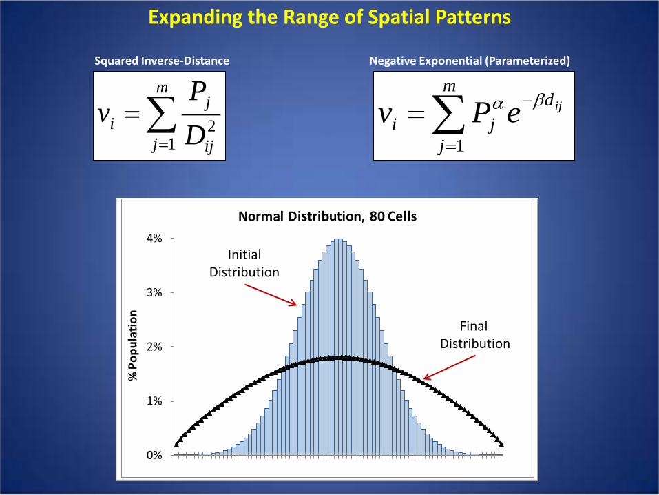
Limited Range of Spatial Patterns The methodology forces a single spatial pattern to evolve over time:

dispersion

This pattern is the result of a fixed distance-decay function

0%

1%

2%

3%

4%

% P

opul

atio

n

Normal Distribution, 80 Cells

t(0)Stability

Final Distribution

Initial Distribution

Expanding the Range of Spatial Patterns

∑=

−=m

j

dji

ijePv1

βα∑=

=m

j ij

ji D

Pv

12

Squared Inverse-Distance Negative Exponential (Parameterized)

Border Effects

Low

High

Projected Population Distribution: NCAR Model, 2100

Modifications: Removing Boundary Effects

A. Base-year

∑=

−=m

j

djii

ijePav1

βα

∑=

−=m

j

dji

ijePv1

βα

Original

Adjusted

mvvv

a i

i

i

−−=

min1

Adjustment Factor

Rural/Urban Boundary Problems

The urban/rural “cliff” effect results from: Classification and separate allocation to urban and rural cells

We eliminate this problem by:

1. Allowing urban and rural population to exist in the same cell. 2. Allocating urban and rural change across all cells.

0%

1%

2%

3%

4%

5%

6%

7%

% P

opul

atio

n

Normal Distribution

t(0) - Urban

t(0) - Rural

t(100) - Urban

t(100) - RuralFinal Distribution

Initial Distribution

Urban/Rural Border

Population Loss is Missallocated

Allocation to Areas Unsuitable for Human Habitation

∑=

−=m

j

djiii

ijePlav1

βα

Smoothing effect of larger windows

Larger windows lead to a smoother potential surface, a result of the wider influence of large urban populations. The result is a more rapid diffusion of the population. Similar to smoothing that results from the repeated application of a moving average window. The larger the window the faster the movement towards uniformity.

Windows

Spatial Stability in the 2-D Hypothetical Model

Population Change; Adjusted vs. Unadjusted 2D Hypothetical Scenario

Potential vs. Inverse Potential Allocation of Population Loss

Historical Data Test: Parameter Estimates

Interpretation of parameter estimates: Relative measure of the change in variability in the spatial distribution of the population.

y = 11516e-0.021x

R² = 0.8516

y = 22593e-0.026x

R² = 0.8377

0

2

4

6

8

10

12

14

16

18

20

0 50 100 150 200

Popu

latio

n Ch

ange

(000

s)

Distance to Urban Center (km)

Border

Interior

Expon. (Border)

Expon. (Interior)

Border Effects: El Paso Example

y = 14497e-0.023x

R² = 0.9771

y = 16186e-0.024x

R² = 0.9669

0

2

4

6

8

10

12

14

16

18

20

0 50 100 150 200

Popu

latio

n Ch

ange

(000

s)

Distance to Urban Center (km)

Border

Interior

Expon. (Border)

Expon. (Interior)

IIASA NCAR

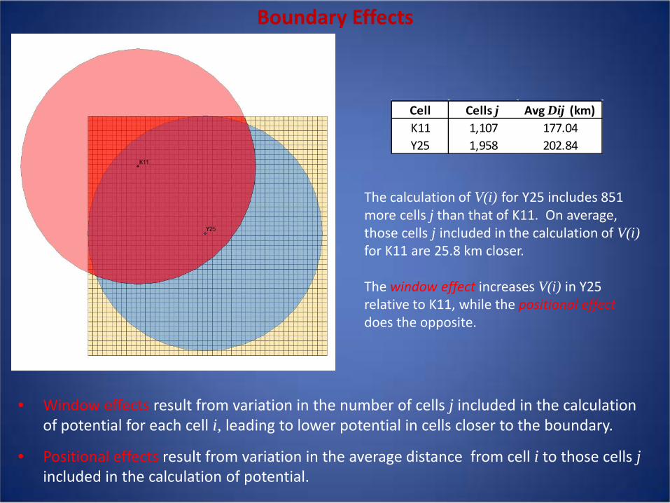
Boundary Effects

• Window effects result from variation in the number of cells j included in the calculation of potential for each cell i, leading to lower potential in cells closer to the boundary.

• Positional effects result from variation in the average distance from cell i to those cells j included in the calculation of potential.

Cell Cells j Avg Dij (km)K11 1,107 177.04Y25 1,958 202.84

The calculation of V(i) for Y25 includes 851 more cells j than that of K11. On average, those cells j included in the calculation of V(i) for K11 are 25.8 km closer. The window effect increases V(i) in Y25 relative to K11, while the positional effect does the opposite.

The Window Effect

The window effect increases potential in red cells relative to blue cells.

0

500

1000

1500

2000

A1 B2 C3 D4 E5 F6 G7 H8 I9 J10

K11

L12

M13

N14

O15 P1

6Q

17 R18

S19

T20

U21

V22

W23 X2

4Y2

5

Cont

ribui

ng ce

lls j

Cell i

Number of cells j contributing to potential

Cells

175

180

185

190

195

200

205

A1 B2 C3 D4 E5 F6 G7 H8 I9 J10

K11

L12

M13

N14

O15 P1

6Q

17 R18

S19

T20

U21

V22

W23 X2

4Y2

5

Aver

age

Dij

Cell i

Average distance to contributing cells j

Avg Dij

The Positional Effect

The positional effect increases potential in red cells relative to blue cells.

0

0.02

0.04

0.06

0.08

0.1

0.12

0.14

0.16

0.18

A1 B2 C3 D4 E5 F6 G7 H8 I9 J10

K11

L12

M13

N14

O15 P1

6Q

17 R18

S19

T20

U21

V22

W23 X2

4Y2

5

V(i)

Cell i

Potential

Potential

Boundary Effects on Potential

NCAR Projections: New York (or other), A2 and B2 Scenarios

NCAR A2 Scenario, 2100 NCAR B2 Scenario, 2100