1

Modeling Supply and Demand in the Chinese Automobile Industry1

Yuan Chen, C.-Y. Cynthia Lin Lawell, Erich J. Muehlegger, and James E. Wilen

June 2017

Abstract China is experiencing rapid economic growth and, along with it, rapid growth in vehicle ownership. The rapid growth in vehicle ownership and vehicle usage is linked to increasing global warming, emissions, air pollution, and other problems. We analyze the supply and demand for automobiles in China, and the effects of government policy on the supply and demand for alternative vehicles. To do so, we develop and estimate a structural econometric model of a mixed oligopolistic differentiated products market that allows different consumers to vary in how much they like different car characteristics on the demand side and that allows state-owned automobile companies to have different objectives than private automobile companies on the supply side. We apply our model to a comprehensive data set on the sales, prices, and characteristics of the majority of vehicle makes and models in China, including electric vehicles, hybrid vehicles, and alternative-fueled vehicles. The parameters we estimate enable us to better understand what factors affect the demand and cost of vehicles in China, and how consumers in China trade off various vehicle characteristics (such as fuel efficiency, whether the vehicle is an electric vehicle, etc.) with each other and with price. We use the model to simulate the demand and cost for new vehicles, and also the effects of various government policies on demand, cost, and welfare.

Keywords: automobile market, China, alternative vehicles, random coefficients model of demand, mixed oligopoly JEL codes: L62, L13, Q58

1 Chen: University of California at Davis; yuachen@ucdavis.edu. Lin Lawell: University of California at Davis; cclin@primal.ucdavis.edu. Muehlegger: University of California at Davis; emuehlegger@ucdavis.edu. Wilen: University of California at Davis; wilen@primal.ucdavis.edu. We thank Yunshi Wang, Jim Bushnell, Michael Canes, Yueyue Fan, Lew Fulton, Hamed Ghoddusi, Khaled Kheiravar, Shanjun Li, Patrick McCarthy, Joan Ogden, Yueming (Lucy) Qiu, Stephen Ryan, John Rust, Jim Sallee, Ashish Sen, Dan Sperling, and James Sweeney for helpful comments and discussions. We also benefited from comments from seminar participants at the UC-Davis Sustainable Transportation Energy Pathways research seminar; and conference participants at the U.S. Association for Energy Economics (USAEE) North American Conference, the Transportation Research Forum Annual Conference, Interdisciplinary Ph.D. Workshop in Sustainable Development (IPWSD) at Columbia University, and the University of California at Davis Sustainable Transportation Energy Pathways Symposium. We are grateful to Xinbiao Gu for helping us collect the data. We received financial support from the China Center for Energy and Transportation of the UC-Davis Institute of Transportation Studies, an ITS-Davis Travel Grant, and a UC-Davis Graduate Student Travel Award. Lin Lawell is a member of the Giannini Foundation of Agricultural Economics. All errors are our own.

2

1. Introduction

China is experiencing rapid economic growth and, along with it, rapid growth in vehicle

ownership. Evidence from Chinese cities suggests average annual growth rates in per capita

vehicle ownership of 10% to 25% (Darido, Torres, and Mehndiratta, 2014). According to data

from the China Statistical Yearbook, vehicle ownership increased by nearly 56 times between 1990

and 2011. The rapid growth in vehicle ownership and vehicle usage is linked to increasing global

warming, emissions, air pollution, and other problems.

For our research, we are developing and estimating a structural econometric model to

estimate demand and cost parameters for all vehicles in China. Our structural econometric model

of a mixed oligopolistic differentiated products market allows different consumers to vary in how

much they like different car characteristics on the demand side and that allows state-owned

automobile companies to have different objectives than private automobile companies on the

supply side. We apply our model to annual data we have collected on sales, prices, and

characteristics of the majority of vehicle makes and models in China, including electric vehicles,

hybrid vehicles, and alternative-fueled vehicles, over the period 2004 to 2013. Our model enables

us to estimate demand- and cost-side parameters, own- and cross-price elasticities, markups, and

variable profits for alternative vehicles.

The parameters we are estimating enable us to better understand what factors affect the

demand and cost of vehicles in China, and how consumers in China trade off various vehicle

characteristics (such as fuel efficiency, whether the vehicle is an electric vehicle, etc.) with each

other and with price. We use the model to simulate the demand and cost for new vehicles, and

also the effects of various government policies on demand, cost, and welfare.

3

Our structural econometric model has several advantages over a survey approach. First,

econometric models are estimated using actual data on actual vehicle purchase decisions, and

therefore may be more accurate a depiction of consumer preferences, since these preferences are

revealed by the actual decisions they make. In contrast, surveys are based on self-reported

responses to questions and may be subject to many errors and biases that cause these responses to

be inaccurate representations of the truth.

A second advantage of our econometric approach over a survey approach is that we

estimate our econometric models using a comprehensive data set we have collected and

constructed on sales, prices, and characteristics of the majority of vehicle makes and models in

China, and will therefore base our models and analysis on the vehicle purchase decisions of all

vehicle owners in China, not just those of the consumers that are surveyed. Our comprehensive

data set not only provides more information, but also is not subject to sample selection issues that

would plague a survey of a sample of the population.

A third advantage of our econometric approach over a survey approach is that our

econometric model enables us to statistically control for multiple factors that may affect vehicle

purchase decisions, including price; vehicle characteristics such as fuel economy, horsepower, and

size; and consumer characteristics in a quantitative and rigorous manner.

A fourth advantage of the structural model is that the parameters we are estimating enable

us to calculate consumer utility, firm profits, and welfare.

A fifth advantage of our structural econometric approach is that it enables us to estimate

standard errors and confidence intervals for our parameters, and therefore to ascertain whether our

parameters are statistically significant.

4

A sixth advantage of our structural econometric approach is that we can use the estimated

parameters to simulate demand, supply, and welfare under counterfactual policy scenarios. These

counterfactual policy simulations will enable us to analyze the effects of vehicle-related policies

in China, including those regarding alternative vehicles.

Our research builds on the work of Berry, Levinsohn and Pakes (1995), who develop a

model for empirically analyzing demand and supply in differentiated products markets and then

apply these techniques to analyze the equilibrium in the U.S. automobile industry. Their

framework enables one to obtain estimates of demand and cost parameters for a class of

oligopolistic differentiated products markets. Unlike traditional logit demand models, their

random coefficients model allows for interactions between consumer and product characteristics,

thus generating reasonable substitution patterns. Estimates from their framework can be obtained

using only widely available product-level and aggregate consumer-level data, and they are

consistent with a structural model of equilibrium in an oligopolistic industry. They apply their

techniques to the U.S. automobile market, and obtain cost and demand parameters for (essentially)

all models marketed over a twenty-year period. On the cost side, they estimate cost as a function

of product characteristics. On the demand side, they estimate own- and cross-price elasticities as

well as elasticities of demand with respect to vehicle attributes (such as weight or fuel efficiency).

We innovate upon the Berry et al. (1995) work by developing a model of the Chinese

automobile market; by including alternative vehicles so that in addition to cost and demand

parameters relating to gasoline-fueled vehicles, cost and demand parameters relating to alternative

vehicles can be estimated; and by modeling the behavior of not only private automobile companies

but also the state-owned automobile companies in China.

5

Our research is significant for industry, government, society, academia, and NGOs. Our

model of the demand and cost in the Chinese automobile market will be significant for industry,

particularly car manufacturers interested in better targeting cars, including alternative vehicles, for

the Chinese market. Our estimates of the factors that affect demand and supply in the Chinese

automobile market is significant for policy-makers interested in developing incentive policies to

increase market penetration of alternative vehicles with potential environmental and climate

benefits.

2. Background

In 2009, China’s automobile market became the largest in the world, surpassing the U.S.

automobile market both in sales and production. The annual gross product of the China’s

automobile industry has exceeded 5% of the country’s annual GDP every year since 2002, and

was as high as 7.4% of its GDP in 2010.2

The Chinese automobile industry underwent several phases of growth since the start of

China’s economic reform in 1978. At that time, automobile manufacturing was very low in

productivity. In the year 1980, total vehicle output was around five thousand vehicles only. As

incomes grew, household demand for passenger vehicle grew rapidly, which resulted in a large

amount of cars being imported to China. In order to protect the vulnerable and immature domestic

Chinese automobile industry, tariffs were set as high as 250% (Li, Xiao and Liu, 2015).

Several large state-owned automobile enterprises in China tried to partner with foreign auto

manufacturers to form joint ventures to increase their capacity and enhance their technical

2 These statistics were calculated using GDP data from the National Bureau of Statistics of China and automobile industry gross product data from Chinese Automobile Industry Yearbook.

6

capabilities. However, foreign ownership was capped at 50% to protect domestic producers. In

1994, China’s National Development and Reform Commission (NDRC) initiated an automobile

industry policy encouraging state-owned firms to partner with international car makers to form

joint ventures (Li, Xiao and Liu, 2015). Following this policy, more joint ventures were formed

between large state-owned automobile companies and foreign auto manufacturers (Li, Xiao and

Liu, 2015). Meanwhile, local and private producers also entered the market.

In 2001, China entered the World Trade Organization (WTO). In order to fulfill its

commitment under the WTO, the Chinese government gradually cut the tariffs on foreign

automobiles from 100% to 25% during the 5-year transition period. However, the market shares

of imports further dropped from about 6% in 2001 to 3% in 2006 and it has stayed at that level

since then (Li, Xiao and Liu 2015).

The Chinese manufacturers of passenger vehicles can be categorized into two different

types: indigenous-brand manufacturers, such as BYD, Geely, and Chery; and joint ventures

between domestic manufacturers and foreign manufacturers, such as Shanghai Automotive

Investment Company (BAIC) with Hyndai, and Dongfeng with Honda.

In Figure A1 in Appendix A, adapted from Hu, Xiao and Zhou (2014), we present the

market structure of the Chinese automobile industry. The car makers in large boxes are the top

state-owned automobile groups in China. The ones in small isolated boxes at the bottom are

indigenous local makers. According to Chinese automobile policy, a Chinese automobile company

can form joint ventures with multiple foreign car manufacturers. For example, Shanghai Auto has

cooperated with General Motors and Volkswagen. Dofeng Motors partners with Nissan, Kia, and

PSA. On the other hand, under Chinese policy, a foreign car manufacturer is only allowed to form

7

joint ventures with up to two Chinese automobile companies.3 For example, Honda partners with

both Donfeng Group and Guangdong Auto. Toyota, another Japanese automobile firm, cooperates

with both Fist Auto Work and Guangdo Auto. Besides large stated-owned auto groups, private

car makers also partner with foreign makers. Huachen Auto cooperates with BMW. Joint ventures

with international car companies account for two thirds of the passenger vehicle market, with the

rest mostly taken up by indigenous brands (Li, Xiao and Liu, 2015).

Figure A2 in Appendix A presents the location of the automobile firms listed in Figure A1

in Appendix A. Most of the automobile firms are located along the east of the continent. Two of

the “China Automobile Group Four” are located in the east, with First Auto Work in the northeast,

and Shanghai Automotive Investment Company (SAIC) in the Southeast. For the other two,

Dongfeng Group is in the middle east of the country, while Chang’an Automobile Group is in

central China. Two large indigenous firms Geely and Chery are located in the southeast part of

China.

In 2005, CAAM, the statistical organization of the Chinese automobile industry that

categorizes vehicles, reclassified vehicles into two broad categories: passenger vehicles and

commercial vehicles. CAAM further divided passenger vehicle into four categories: Basic

Passenger Vehicle (BPV), Sports Utility Vehicle (SUV), Multi-purpose Vehicle (MPV), and

others (such as crossovers). In 2012, according to the China Automobile Industry Year Book, the

total Basic Passenger Vehicle (BPV) output is 10.767 million and that for Multi-purpose Vehicle

(MPV) and Sports Utility Vehicle (SUV) is 491.896 thousand and 1.999 million respectively. The

3 According to “Chinese Automobile Industry Development Policy, 2009 edited edition”. http://www.china.com.cn/policy/txt/2009-08/31/content_18430768_5.htm

8

total output and sales for passenger vehicle in 2012 is 13.258 million and 13.239 million,

respectively.

According to China’s National Bureau of Statistics, from 2004 to 2014, the total number

of civil passenger vehicles owned in China increased from 17.35 million to 123.27 million, with

an annual growth rate of 21.69%. The total number of civil vehicle owned in China, including civil

trucks, was 145.98 million in 2014.

In September 2004, China introduced its first fuel economy standards for light duty

passenger vehicles (GB 19578-2004), targeting a fuel consumption of 6.9 L/100km by 2015, which

translates to an estimated 167 g/km of CO2 emissions. The standards were initially outlined in two

phases with different national standards of “limits of Fuel Consumption of Passenger Cars”. The

national standard limits are set for 16 categories of curb weights and also differentiates manual

transmission from automatic transmission.

The first phase began in July 2005 for new vehicle production, and a year later for existing

vehicle production. Phase 2 began in January 2008 for new vehicle production, and full segment

production compliance was implemented in 2009.

The cars initially included in the fuel economy standard were passenger cars, SUVs, and

light commercial vehicles (LCVs). These vehicles are collectively defined as M1-type vehicles

by the EU, and are defined in the Chinese standard as vehicles with a minimum speed of 50 km/h

and a maximum weight of 3500 kg.

The third phase of the passenger vehicle fuel economy standard includes Corporate

Average Fuel Consumption (CAFC) target (GB 27999-2011), which went into effect in 2012 and

is intended to bind in 2015. Together with the passenger car fuel limits standard (GB 19678-2004),

CAFC is designed to realize an ambitious average fuel consumption target of 6.9 L/100km by

9

2015. The fourth phase recently released is providing gradual implementation guidelines towards

a 2020 5.0 L/100km binding target.

The CAFC uses vehicle model, year, and annual sales to calculate the following weighted

average for fuel consumption based on the New European Driving Cycle (NEDC):

i i

i

ii

FC VCAFC

V

⋅=∑∑

,

where iFC is the fuel consumption of model i and iV is the annual sales of model i.

The government sets higher weights for alternative fuel vehicles to encourage their

production. Until 2015, in the CAFC calculation, a multiplier of 5, 5, 5, 3 of the quantity sales are

used for pure-electric, fuel-cell electric, plug-in hybrid, and energy saving vehicles respectably.

The weights gradually decrease thereafter.4

The CAFC target CAFCT is based on individual vehicle fuel consumption targets, which use

the quantity of annual sales of each model to calculate a weighted average as follows:

i ii

CAFCi

i

T VT

V

⋅=∑∑

,

where iT is the fuel consumption target of model i and iV is the annual sales of model i.

The national standard (GB 27999) target implementation status is indicated by CAFC

CAFCT

.

The CAFC requirement was enacted in 2012 and allows automobile manufacturers until 2015 to

4 2015 annual report of Chinese passenger vehicle fuel consumption 2015 by Innovation Center for Energy and Transportation

10

gradually reduce the fuel consumption levels (3% each year), towards the CAFC binding period

starting in 2015 (100% compliance).

In addition to fuel economy standards, in 2010 the Chinese government established a

project called “energy saving projects”, which uses a fiscal subsidy to encourage energy saving.

Some autos with low displacement (less than 1.6L) will receive a subsidy (directly to the car

makers) such that the market price is the price after subsidized.5

3. Literature Review

3.1. Structural econometric models of demand and supply in differentiated products markets

The first strand of literature we build upon is that on structural econometric models of

demand and supply in differentiated products markets. Berry (1994) develops techniques for

estimating discrete choice demand models which involve “inverting” the market share equation to

find the implied mean levels of utility for each good. Goldberg (1995) develops and estimates a

model of the U.S. automobile industry in which demand is modeled with a discrete choice model

estimated using micro data from the Consumer Expenditure Survey, and supply is modeled as an

oligopoly with differentiation. Feenstra and Levinsohn (1995) demonstrate how to estimate a

model of oligopoly pricing when products are multi-dimensionally differentiated.

Berry, Levinsohn and Pakes (1995) develop techniques for empirically analyzing demand

and supply in differentiated products markets and then apply these techniques to analyze the

equilibrium in the U.S. automobile industry. The framework they present enables one to obtain

estimates of demand and cost parameters for a class of oligopolistic differentiated products

5 Announcement published by the Ministry of Finance of the People’s Republic of China. http://jjs.mof.gov.cn/zhengwuxinxi/zhengcefagui/201006/t20100601_320724.html

11

markets, using only widely available product-level and aggregate consumer-level data, which are

consistent with a structural model of equilibrium in an oligopolistic industry.

Innovations, extensions, and refinements to Berry, Levinsohn and Pakes (1995) have been

made by Petrin (2002), Berry, Levinsohn and Pakes (2004),Hoderlein, Klemela and Mammen

(2008), Dube, Fox and Su (2012), Knittel and Metaxoglou (2014), Reynaert and Verboven (2014),

Berry and Haile (2014), Berry and Haile (2016), Bajari et al. (2015), and Armstrong (2016).

3.2. Vehicle markets and policy

The second strand of literature we build upon is that on vehicle markets and policy,

particularly for alternative vehicles. A more detailed review of this literature is provided in Chen,

Lin Lawell and Wang (2017).

One sub-branch of this literature is the literature on vehicle demand. Sallee, West and Fan

(2016) measure consumers’ willingness to pay for fuel economy using a novel identification

strategy and high quality microdata from wholesale used car auctions. Anderson and Sallee (2016)

present a simplified model of car choice that allows them to emphasize the relationships between

fuel economy, other car attributes, and miles traveled.

Understanding demand in the new plug-in hybrid electric vehicle (PHEV) market is critical

to designing more effective adoption policies. Sheldon, DeShazo and Carson (2016) use stated

preference data from an innovative choice experiment to estimate demand for PHEVs relative to

battery electric vehicles (BEVs) and to explore heterogeneity in demand for these vehicles.

Deshazo, Sheldon and Carson (forthcoming) assess the performance of alternative rebate designs

for plug-in electric vehicles.

12

Li and Zhou (2015) examine the dynamics of technology adoption and critical mass in

network industries with an application to the U.S. electric vehicle (EVs) market, which exhibits

indirect network effects in that consumer EV adoption and investor deployment of public charging

stations are interdependent.

Holland, Mansur, Muller, and Yates (2016) combine a theoretical discrete-choice model of

vehicle purchases, an econometric analysis of electricity emissions, and the AP2 air pollution

model to estimate the geographic variation in the environmental benefits from driving electric

vehicles.

Another sub-branch is the literature on the effects of government policy on vehicle demand,

particularly for alternative vehicles. Gallagher and Muehlegger (2011) study the relative efficacy

of state sales tax waivers, income tax credits, and non-tax incentives to induce consumer adoption

of hybrid-electric vehicles. They find that the type of tax incentive offered is as important as the

generosity of the incentive. Beresteanu and Li (2011) analyze the determinants of hybrid vehicle

demand, focusing on gasoline prices and income tax incentives. They show that the cost

effectiveness of federal tax programs can be improved by a flat rebate scheme. Sallee (2011)

estimates the incidence of tax incentives for the Toyota Prius. Transaction microdata indicate that

both federal and state incentives were fully captured by consumers. Jacobsen and van Benthem

(2015) estimate the sensitivity of scrap decisions to changes in used car values and show how this

“scrap elasticity” produces emissions leakage under fuel efficiency stands, a process known as the

Gruenspecht effect.

Another sub-branch is the literature on vehicle supply, and the effects of policies on vehicle

supply. Heutel and Muehlegger (2015) study the effect of differences in product quality on new

technology diffusion. Using detailed vehicle specifications, Ullman (2016) analyzes the impact

13

identifiable vehicle characteristics and technological progress has on fleet economy by vehicle

type and class. He finds evidence that the stringent footprint-based standards create manufacturer

incentive to increase vehicle size to lower the burden of compliance, which undermines the

standards’ potential to create expected fuel savings and lower emissions levels. Miravete, Moral

and Thurk (2016) estimate a discrete choice oligopoly model of horizontally differentiated

products using Spanish automobile registration data to assess the degree to which vehicle

emissions policies impact the automobile industry, focusing on the European market where diesels

are popular.

Another sub-branch is the literature on government policies related to vehicles. Despite

widespread agreement that a carbon tax would be more efficient, many countries use fuel economy

standards to reduce transportation-related carbon dioxide emissions. Davis and Knittel (2016) pair

a simple model of the automakers' profit maximization problem with unusually-rich nationally

representative data on vehicle registrations to estimate the distributional impact of U.S. fuel

economy standards. The key insight from the model is that fuel economy standards impose a

constraint on automakers which creates an implicit subsidy for fuel-efficient vehicles and an

implicit tax for fuel-inefficient vehicles.

Economists promote energy taxes as cost-effective. But policy-makers raise concerns

about their regressivity, or disproportional burden on poorer families, preferring to set energy

efficiency standards instead. Levinson (2016) first show that in theory, regulations targeting

energy efficiency are more regressive than energy taxes, not less. He then provides an example in

the context of automotive fuel consumption in the United States: taxing gas would be less

regressive than regulating the fuel economy of cars if the two policies are compared on a revenue-

equivalent basis.

14

Sallee and Slemrod (2012) analyze notches in fuel economy policies, which aim to reduce

negative externalities associated with fuel consumption. They provide evidence that automakers

respond to notches in the Gas Guzzler Tax and mandatory fuel economy labels by precisely

manipulating fuel economy ratings so as to just qualify for more favorable treatment. Jacobsen

(2013) employs an empirically estimated model to study the equilibrium effects of an increase in

the US corporate average fuel economy (CAFE) standards. Kellogg (2017) shows that the

implications of gasoline price volatility for the design of fuel economy policies. Bento, Gillingham

and Roth (2017) examine the effect of fuel economy standards on vehicle weight dispersion and

accident fatalities

3.3. Vehicle markets and policy in China

The third strand of literature we build upon is that on vehicle markets and policy in China.

Huo et al. (2007) develop a methodology to project growth trends of the motor vehicle population

and associated oil demand and carbon dioxide emissions in China through 2050. Projections show

that by 2030 China could have more highway vehicles than the United States has today.

China’s vehicle population is widely forecasted to grow 6-11% per year into the

foreseeable future. Barring aggressive policy intervention or a collapse of the Chinese economy,

Wang, Teter and Sperling (2011) suggest that those forecasts are conservative. They analyze the

historical vehicle growth patterns of seven of the largest vehicle producing countries at comparable

times in their motorization history. They estimate vehicle growth rates for this analogous group of

countries to have 13-17% per year- roughly twice the rate forecasted for China by others. Applying

these higher growth rates to China results in the total vehicle fleet reaching considerably higher

15

volumes than forecasted by others, implying far higher global oil use and carbon emissions than

projected by the International Energy Agency and others.

Lin and Zeng (2013) estimate the price and income elasticities of demand for gasoline in

China. Their estimates of the intermediate-run price elasticity of gasoline demand range between

-0.497 and -0.196, and their estimates of the intermediate-run income elasticity of gasoline demand

range between 1.01 and 1.05. They also extend previous studies to estimate the vehicle miles

traveled (VMT) elasticity and obtain a range from -0.882 to -0.579.

Lin and Zeng (2014) calculate the optimal gasoline tax for China using a model developed

by Parry and Small. They calculate the optimal adjusted Pigovian tax in China to be $1.58 /gallon

which is 2.65 times more than the current level. Of the externalities incorporated in this Pigovian

tax, the congestion costs are taxed the most heavily, at $0.82/gallon, followed by local air pollution,

accident externalities, and finally global climate change.

Hu, Xiao and Zhou (2014) apply a non-nested hypothesis test methodology to data on

Chinese passenger vehicles to identify whether price collusion exists within corporate groups or

across groups. Their empirical results support the assumption of Bertrand Nash competition in the

Chinese passenger-vehicle industry. No evidence for within or cross-group price collusion is

found. In addition, the policy experiments show that indigenous brands will gain market shares

and profits if within group companies merge.

Xiao and Ju (2014) explore the effects of consumption-tax and fuel-tax adjustments in the

Chinese automobile industry. Their empirical findings suggest that the fuel tax is effective in

decreasing fuel consumption at the expense of social welfare, while the consumption tax does not

significantly affect either fuel consumption or social welfare.

16

Li, Xiao and Liu (2015) document the evolution of price and investigate the sources of

price decline in the Chinese automobile market, paying attention to both market structure and cost

factors. They estimate a market equilibrium model with differentiated multiproduct oligopoly

using market-level sales data in China together with information from household surveys. Their

counterfactual simulations show that (quality-adjusted) vehicle prices have dropped by 33% from

2004 to 2009. The decrease in markup from intensified competition accounts for about one third

of this change and the rest comes from cost reductions through learning by doing and other

channels.

Liu and Lin Lawell (2017) examine the effects of public transportation and the built

environment on the number of civilian vehicles in China. They use a 2-step GMM instrumental

variables model and apply it to city-level panel data over the period 2001 to 2011. The results

show that increasing the road area increases the number of civilian vehicles. In contrast, increasing

the public transit passenger load decreases the number of civilian vehicles. However, the effects

vary by city population. For larger cities, increases in the number of public buses increase the

number of civilian vehicles, but increases in the number of taxis and in road area decrease the

number of civilian vehicles. They also find that land use diversity increases the number of civilian

vehicles, especially in the higher income cities and in the extremely big cities. Finally, they find

no significant relationship between civilian vehicles and per capita disposable income except in

mega cities.

Both market-based and non-market based mechanisms are being implemented in China’s

major cities to distribute limited vehicle licenses as a measure to combat worsening traffic

congestion and air pollution. While Beijing employs non-transferable lotteries, Shanghai uses an

auction system. Li (2016) empirically quantifies the welfare consequences of the two mechanisms

17

by taking into account both allocation efficiency and automobile externalities post-allocation. His

analysis shows that different allocation mechanisms lead to dramatic differences in social welfare.

Although the lottery system in Beijing has a large advantage in reducing externalities from

automobile use than a uniform price auction, the advantage is offset by the significant welfare loss

from misallocation. The lottery system forewent nearly 36 billion RMB (or $6 billion) in social

welfare in Beijing in 2012 alone. A uniform-price auction would have generated 21.6 billion RMB

to Beijing municipal government, more than covering all the subsidies to the local public transit

system.

3.4. Mixed oligopoly

The fourth strand of literature we build upon is that on mixed oligopoly. A mixed oligopoly

is defined as an oligopolistic market structure with a relatively small number of firms for which

the objective of at least one firm differs from that of other firms (De Fraja and Delbono, 1990), as

opposed to a private oligopoly in which all firms have the objective of profit maximization.

Usually in a mixed oligopoly there is a public firm competing with a multitude of profit-

maximizing firms (Poyago-Theotoky, 2001).

De Fraja and Delbona (1989) study a situation in which private and public firms compete

both using only market instruments. When talking about public and private firms, they think of

firms which pursue different objectives. They find that nationalization is always socially better

than Stackelberg leadership, which is in turn socially better than Cournot-Nash behavior. If there

is no way of avoiding competition with a public firm, private entrepreneurs would prefer the public

firm to behave as a Stackelberg leader.

18

De Fraja and Delbona (1990) examine a case of mixed oligopoly which is particularly

interesting from the point of view of economic and industrial policy: a market in which at least

one publicly owned firm cohabits which at least one private firm. A market where there are both

private and public firms is then a mixed oligopoly because the firms owned by private agents aim

to maximize profits, whereas the publicly owned firms are interested in optimizing social targets.

There are two broad results which emerge from the models considered in this survey. First, the

public authority can fruitfully use the public firms as an instrument towards the achievement of its

goals, namely the increase of social welfare. Second, in general, it does not seem to be optimal for

the public authority to instruct the public firms to take decisions which result in equality between

price and marginal cost, either because of a budget constraint, or because the maximum social

welfare is reached when price is higher than public marginal cost.

Since previous articles on mixed oligopoly did not include foreign private firms, Fjell and

Pal (1996) consider a mixed oligopoly model in which a state-owned public firm competes with

both domestic and foreign private firms. The effect on the equilibrium involves a lower price and

a different allocation of production. They also discuss issues such as the effects of an open door

policy allowing foreign firms to enter and the effects of foreign acquisition of domestic firms.

White (1996) examines the use of output subsidies in the presence of a mixed oligopoly.

He finds that if subsidies are used in a simultaneous-moves oligopoly and the industry is

subsequently privatized, there is a reduction in social welfare. Moreover, both in the private

oligopoly and in the mixed oligopoly, the optimal output subsidy is identical.

Poyago-Theotoky (2001) provide a much stronger “irrelevance” result with respect to

firms’ moves and market structure in the presence of output subsidization. In addition to a private

oligopoly and a mixed oligopoly where all firms make their output decisions simultaneously, they

19

consider the case of the public firms acting as a Stackelberg leader. They show that the optimal

output subsidy is identical and profits, output and social welfare are also identical irrespective of

whether (i) the public firm moves simultaneously with the private firms or (ii) the public firm acts

as Stackelberg leader or (iii) all firms behave as profit-maximizers.

De Fraja (2009) argues that whether a taxpayer financed subsidy to some suppliers

(typically the public ones) is tantamount to “unfair” competition should be assessed with the

understanding of the nature of the objective function of the providers: behavior which would be

deemed anti-competitive for a profit maximizing oligopolist, may be in line with the objective

function of a public, welfare-maximizing supplier. On the other hand, where the presence of public

suppliers bestows a positive externality on the private suppliers, then a taxpayer financed subsidy

distributed asymmetrically to the players in the sector according to their ownership may benefit all

suppliers, private and public alike.

In Lutz and Pezzino’s (2010) setting, a private and a public firm face fixed quality-

dependent costs of production and compete first in quality and then either in prices or in quantities.

In the long run the public firm targets welfare maximization whereas the private firm maximizes

profits. In the short run both firms compete in prices or quantities to maximize profits. They

conclude that mixed competition is always socially desirable compared to a private duopoly

regardless of the type of competition in the short run and the equilibrium quality ranking. In

addition, mixed competition seems to be a more efficient regulatory instrument than the adoption

of a minimum quality standard.

Bennett and La Manna (2012) also consider a mixed oligopoly with free entry by private

firms, assuming that a public firm maximizes an increasing function of output, subject to a break-

even constraint. An irrelevance result is obtained: whenever a mixed oligopoly is viable, then

20

aggregate output, aggregate costs and welfare are the same with and without the public firm.

However, replacing a viable mixed oligopoly with a public monopoly yields higher net welfare.

Haraguchi and Matsumura (2016) revisit the classic discussion comparing price and

quantity competition, but in a mixed oligopoly in which one state-owned public firm competes

against private firms. It has been shown that in a mixed duopoly, price competition yields a larger

profit for the private firm. They adopt a standard differentiated oligopoly with a linear demand and

find that regardless of the number of firms, price competition yields higher welfare, however, the

profit ranking depends on the number of private firms. They also endogenize the price-quantity

choice and find that Bertrand competition can fail to be an equilibrium, unless there is only one

private firm.

A related literature is that on the objectives of state-owned firms. Ghandi and Lin (2012)

model the dynamically optimal oil production on Iran’s offshore Soroosh and Nowrooz fields,

which have been developed by Shell Exploration through a buy-back service contract. In

particular, they examine the National Iranian Oil Company’s (NIOC) actual and contractual oil

production behavior and compare it to the production profile that would have been optimal under

the conditions of the contract. They find that the contract’s production profile is different from

optimal production profile for most discount rates, and that the NIOC’s actual behavior is

inefficient- its production rates have not maximized profits. Because the NIOC’s objective is

purported to be maximizing cumulative production instead of the present discounted value of the

entire stream of profits, they also compare the NIOC’s behavior to the production profile that

would maximize cumulative production. They find that even though what the contract dictates

comes close to maximizing cumulative production, the NIOC has not been achieving its own

objective of maximizing cumulative production.

21

4. Econometric Model

4.1. Demand

Our structural econometric model improves upon conventional econometric analysis using

traditional logit models. A traditional logit model of vehicle demand assumes the independence of

irrelevant alternatives, and can therefore generate unrealistic substitution patterns. In a logit

model, if you take away a car model from the choice set, then consumers of that car will buy other

cars according to their market shares. However, in reality, if you remove, say, a luxury car, the

consumers of that luxury car are probably more likely to buy another luxury car than a random

consumer would, even if luxury cars have low market share.

In contrast, the random coefficients demand model of vehicle demand we use addresses

this problem by allowing for interactions between unobserved consumer characteristics and

observed product characteristics, thus allowing different consumers to vary in how much they like

different car characteristics.

Our research builds on the work of Berry, Levinsohn and Pakes (1995), who develop a

model for empirically analyzing demand and supply in differentiated products markets and then

apply these techniques to analyze the equilibrium in the U.S. automobile industry. Their

framework enables one to obtain estimates of demand and cost parameters for a class of

oligopolistic differentiated products markets. Unlike traditional logit demand models, their

random coefficients model allows for interactions between consumer and product characteristics,

thus generating reasonable substitution patterns. Estimates from their framework can be obtained

using only widely available product-level and aggregate consumer-level data, and they are

consistent with a structural model of equilibrium in an oligopolistic industry. They apply their

22

techniques to the U.S. automobile market, and obtain cost and demand parameters for (essentially)

all models marketed over a twenty-year period. On the cost side, they estimate cost as a function

of product characteristics. On the demand side, they estimate own- and cross-price elasticities as

well as elasticities of demand with respect to vehicle attributes (such as weight or fuel efficiency).

Our research innovates upon the Berry et al. (1995) work by developing a model of the

Chinese automobile market; by including alternative vehicles so that in addition to cost and

demand parameters relating to gasoline-fueled vehicles, cost and demand parameters relating to

alternative vehicles can be estimated; and by modeling the behavior of not only private automobile

companies but also the state-owned automobile companies in China.

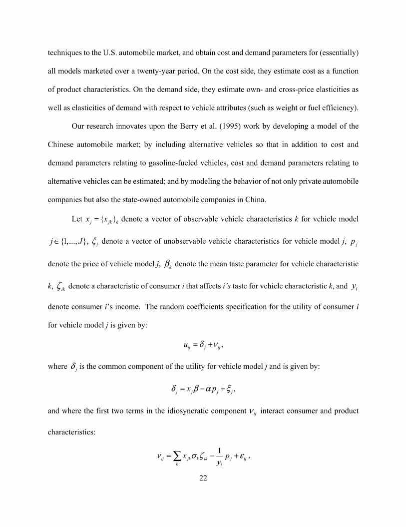
Let { }j jk kx x= denote a vector of observable vehicle characteristics k for vehicle model

{1,..., }j J∈ , jξ denote a vector of unobservable vehicle characteristics for vehicle model j, jp

denote the price of vehicle model j, kβ denote the mean taste parameter for vehicle characteristic

k, ikζ denote a characteristic of consumer i that affects i’s taste for vehicle characteristic k, and iy

denote consumer i’s income. The random coefficients specification for the utility of consumer i

for vehicle model j is given by:

,ij j iju δ ν= +

where jδ is the common component of the utility for vehicle model j and is given by:

,j j j jx pδ β α ξ= − +

and where the first two terms in the idiosyncratic component ijν interact consumer and product

characteristics:

1ij jk k ik j ij

k i

x py

ν σ ζ ε= − +∑ ,

23

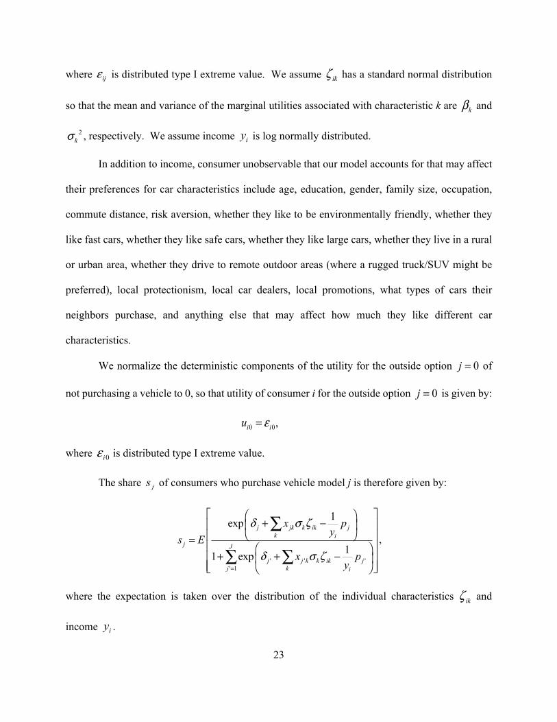
where ijε is distributed type I extreme value. We assume ikζ has a standard normal distribution

so that the mean and variance of the marginal utilities associated with characteristic k are kβ and

2kσ , respectively. We assume income iy is log normally distributed.

In addition to income, consumer unobservable that our model accounts for that may affect

their preferences for car characteristics include age, education, gender, family size, occupation,

commute distance, risk aversion, whether they like to be environmentally friendly, whether they

like fast cars, whether they like safe cars, whether they like large cars, whether they live in a rural

or urban area, whether they drive to remote outdoor areas (where a rugged truck/SUV might be

preferred), local protectionism, local car dealers, local promotions, what types of cars their

neighbors purchase, and anything else that may affect how much they like different car

characteristics.

We normalize the deterministic components of the utility for the outside option 0j = of

not purchasing a vehicle to 0, so that utility of consumer i for the outside option 0j = is given by:

0 0i iu ε= ,

where 0iε is distributed type I extreme value.

The share js of consumers who purchase vehicle model j is therefore given by:

' ' '' 1

1exp

11 exp

j jk k ik jk i

j J

j j k k ik jj k i

x py

s Ex p

y

δ σ ζ

δ σ ζ=

⎡ ⎤⎛ ⎞+ −⎢ ⎥⎜ ⎟

⎝ ⎠⎢ ⎥= ⎢ ⎥⎛ ⎞+ + −⎢ ⎥⎜ ⎟

⎢ ⎥⎝ ⎠⎣ ⎦

∑

∑ ∑,

where the expectation is taken over the distribution of the individual characteristics ikζ and

income iy .

24

Traditional logit and probit models commonly assume that there are no terms in the

idiosyncratic component ijν that interact consumer and product characteristics (i.e., ij ijν ε= ) and

therefore that the variation in consumer tastes enters only through the additive error term ijε ,

which is assumed to be identically and independently distributed across consumers and choices.

However, this strong assumption places very strong restrictions on the pattern of cross-price

elasticities from the estimated model. All properties of market demand, including market shares

and elasticities, are determined solely by the common component of utility jδ . In the automobile

market, for example, this property implies that any pair of cars with the same pair of market shares

will have the same cross-price elasticity with any given third product.

In contrast, in a random coefficients demand model, owing to the interaction between

consumer preferences and product characteristics in ijv , consumers who have a preference for size

will tend to attach a high utility to all large cars, and this will induce large substitution effects

between large cars.

The estimation equation on the demand side is the calculated common component of utility

jδ , which is given by the inverse market share function:

( ) ,j j j j js x pδ β α ξ= − +

where js is the share of consumers who purchase vehicle model j. To derive the inverse market

share function ( )j jsδ , we first compute the expected market share function as a function of the

common components of utility jδ , where the expectation is taken over the distribution of

consumer characteristics, and then invert the expected market share function to derive the common

25

component of utility jδ as a function of market share js via a contracting mapping algorithm.

Following Li (2015), we employ Newton’s method to increase the speed of convergence.

4.2. Supply

On the supply side, we make innovate upon the literature by allowing state-owned

automobile companies to have different objectives from private automobile companies.

We assume a Bertrand (Nash-in-prices) equilibrium among multiproduct firms.

We assume private firms have as their objective that of maximizing profits. Their

objective function is therefore profits ( )π ⋅ , which are given by:

( ) ( ( )) ( )f

j j jj J

p c Msπ∈

⋅ = − ⋅ ⋅∑ ,

where M is the total number of consumers and jc is the marginal cost for vehicle j.

The estimation equation on the supply side for private firms is given by the following

pricing equation for vehicle j:

1p s c−−Δ = ,

where p is a vector of vehicle prices, one for each vehicle j; Δ is a matrix in which kjk

j

sp∂Δ = −∂

if

j and k are produced by the same firm and 0 jkΔ = otherwise; s is the vector of vehicle market

shares; and c is the vector of vehicle marginal costs.

Unlike private firms, state-owned firms may have objectives other than profit

maximization alone. We assume the objective function (utility function) for state-owned firms is

given by the following weighted sum of profits ( )π ⋅ , consumer surplus ( )CS ⋅ , the squared

difference ( )TAR ⋅ between the number of alternative vehicles produced by that firm and a target

26

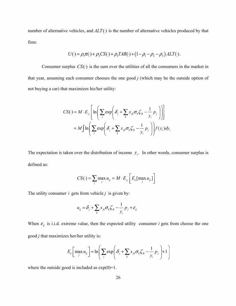
number of alternative vehicles, and ( )ALT ⋅ is the number of alternative vehicles produced by that

firm:

( )1 2 3 1 2 3( ) ( ) ( ) ( ) 1 ( )U CS TAR ALTρ π ρ ρ ρ ρ ρ⋅ = ⋅ + ⋅ + ⋅ + − − − ⋅ .

Consumer surplus ( )CS ⋅ is the sum over the utilities of all the consumers in the market in

that year, assuming each consumer chooses the one good j (which may be the outside option of

not buying a car) that maximizes his/her utility:

1( ) ln exp

1 ln exp ( )

iy j jk k ik jj k i

j jk k ik j i ij k i

CS M E x py

M x p f y dyy

δ σ ζ

δ σ ζ

⎡ ⎤⎛ ⎞⎛ ⎞⋅ = ⋅ + −⎢ ⎥⎜ ⎟⎜ ⎟⎜ ⎟⎢ ⎥⎝ ⎠⎝ ⎠⎣ ⎦

⎛ ⎞⎛ ⎞= + −⎜ ⎟⎜ ⎟⎜ ⎟⎝ ⎠⎝ ⎠

∑ ∑

∑ ∑∫

The expectation is taken over the distribution of income iy . In other words, consumer surplus is

defined as:

( ) max [max ]iij y ijj ji

CS u M E E uε⎡ ⎤⋅ = = ⋅ ⎢ ⎥⎣ ⎦∑

The utility consumer i gets from vehicle j is given by:

1ij j jk k ik j ij

k i

u x py

δ σ ζ ε= + − +∑

When ijε is i.i.d. extreme value, then the expected utility consumer i gets from choose the one

good j that maximizes her/her utility is:

1max ln exp 1ij j jk k ik jj j k i

E u x pyε δ σ ζ

⎛ ⎞⎛ ⎞⎡ ⎤ = + − +⎜ ⎟⎜ ⎟⎜ ⎟⎢ ⎥⎣ ⎦ ⎝ ⎠⎝ ⎠∑ ∑

where the outside good is included as exp(0)=1.

27

Thus,

1( ) ln exp 1

iy j jk k ik jj k i

CS M E x py

δ σ ζ⎡ ⎤⎛ ⎞⎛ ⎞

⋅ = ⋅ + − +⎢ ⎥⎜ ⎟⎜ ⎟⎜ ⎟⎢ ⎥⎝ ⎠⎝ ⎠⎣ ⎦∑ ∑ .

( )TAR ⋅ is the squared difference between the number of alternative vehicles produced by

that firm and a target number of alternative vehicles:

2 2

; ;( )

f f

j jj J j hybrid j J j hybrid

TAR q h Ms h∈ ∈ ∈ ∈

⎛ ⎞ ⎛ ⎞⎛ ⎞ ⎛ ⎞⎜ ⎟ ⎜ ⎟⋅ = − = −⎜ ⎟ ⎜ ⎟⎜ ⎟ ⎜ ⎟⎜ ⎟ ⎜ ⎟⎝ ⎠ ⎝ ⎠⎝ ⎠ ⎝ ⎠

∑ ∑,

where the alternative vehicles target is h , which we assume is the same for all the state-owned

firms for now.

( )ALT ⋅ is the number of alternative vehicles produced by that firm:

; ;( )

f f

j jj J j alt j J j alt

ALT q Ms∈ ∈ ∈ ∈

⋅ = =∑ ∑

The ρ ’s are weights put on each of the possible terms in the state-owned company’s utility

function.

Thus, the pricing equation for the state-owned firms is given by:

1 23 1 2 3

1 1

1( ) (2 ( ) ) (1 ) 1ll nl

p s e M s h cρ ρ ρ ρ ρρ ρ

− ⎡ ⎤⎛ ⎞− Δ − + ⋅ − + − − − Δ ⋅ =⎢ ⎥⎜ ⎟⎝ ⎠⎣ ⎦

∑ ,

where Δ is defined the same as before; lΔ is a matrix in which l ljl

j

sp∂Δ =∂

if fl J l hybrid∈ ∧ ∈

and =0jlΔ otherwise; and e is a vector whose thj element is given by:

28

' ''

1 1

1 ' 1i

j jk k ik jki i

y

j j k k ik jj ki

exp x py y

E

exp x py

δ σ ζ α

δ σ ζ

⎡ ⎤⎛ ⎞⎛ ⎞+ − −⎢ ⎥⎜ ⎟⎜ ⎟

⎢ ⎥⎝ ⎠⎝ ⎠= ⎢ ⎥⎡ ⎤⎛ ⎞⎢ ⎥+ − +⎢ ⎥⎜ ⎟⎢ ⎥⎝ ⎠⎣ ⎦⎣ ⎦

∑

∑ ∑.

For our specification of marginal costs jc , to examine whether forming joint ventures with

international firms would help improve the technology development of the domestic

manufacturers, we include interactions between a “Has international joint venture” (HIJV) dummy

with some of the technology-related car characteristics in our specification for marginal cost jc .

The HIJV dummy equals 1 if the Chinese car company forms a joint venture with any international

car company and 0 otherwise. The technology-related car characteristics we chosen are: “the

dummy for the car j being alternative vehicle”, “fuel efficiency” and “horsepower”.

Furthermore, to examine whether forming a joint venture with international companies

located in different countries will have different effects on helping domestic firms’ technology

improvement, we also include interactions between an “international joint venture country” (IJVC)

dummy and technology-related vehicle characteristics in our specification for marginal cost jc .

The IJVC dummy is equal to 1 if the Chinese car company forms a joint venture with an

international car company headquartered in the country and 0 otherwise. There are six international

joint venture countries: Japan, Germany, Britain, US, South Korea, Sweden, France and Italy. The

technology-related characteristics chosen are “the dummy for the car j being alternative vehicle”,

“fuel efficiency” and “horsepower”.

In 2012, the Corporate Average Fuel Consumption (CAFC) target went into effect, which

might affect firms’ competing strategies. We want to see if a firm that is required to meet the

29

CAFC target experiences a higher marginal cost from producing a car with worse fuel economy

than the target corporate average. We therefore include three fuel economy interaction terms

interactionfuel in the marginal cost jc . The first term is the dummy variable for Phase 3 CAFC

standard. The second is phase 3 national fuel economy standard limit less fuel efficiency and the

last one is the interaction term between phase 3 fuel economy CAFC dummy and the difference

between the phase 3 CAFC standard and fuel efficiency.

Marginal cost jc for car j is therefore given by:

1 2 3j j j int int int jc x w q tech techIJVC fuelγ η ψ ψ ψ ω= + Γ + + + + ⋅ +⋅ ⋅

where w is a joint venture dummy vector, for which the thf element equals one if the maker that

produces good j forms a joint venture with company f ; inttech are the HIJV interaction terms,

including the HIJV dummy interacted with the alternative vehicle dummy, fuel efficiency, and

horsepower; inttechIJVC are the three technology-related characteristics interacting with each of

the IJVC dummies; intfuel are the fuel economy policy interaction terms; and jω are the

unobservable cost variables.

4.3.Econometric Estimation

The parameters to be estimated include the means β of the marginal utility associated with

each particular characteristic, the parameter α in the marginal disutility of price, the cost

parameters γ , the coefficient Γ associated with joint venture companies, the coefficient η on

quantity in marginal cost, the standard deviations σ of the marginal utility associated with each

particular characteristic, the ρ ’s for the weights on different objective terms of state-owned firms

30

and h for target number of alternative vehicle production, and finally the 1ψ on the international

joint venture dummy interaction terms, 2ψ on the international joint venture country interaction

terms, and 3ψ on fuel economy interaction terms in marginal cost.

Because the observed equilibrium prices and quantities are simultaneously determined in

the supply-and-demand system, instrumental variables are needed to address the endogeneity

problem (Goldberger, 1991; Manski, 1995; Angrist et al., 2000; Lin, 2011). Since price and the

market share variables are endogenous in demand and supply, we use instruments for the

endogenous price and market share variables.

The instrumental variables we use in our estimation build on the work of Berry et al. (1995).

We construct two different types of instrumental variables based on each car characteristic: the

number of cars with similar values of the characteristic, and the value of the characteristic for the

car k closest to car j in the value of the characteristic. More specifically, for each characteristic r ,

the first instrumental variable we create is the number of cars that has similar value of attribute r

to car j . Two cars j and k are “similar” in characteristic r if the squared difference in their values

of that characteristic is less than or equal to one tenth of the squared difference between the

maximum and minimum values of that characteristic among all cars:

( )22 1( ) max( ) min( )

10jr kr r rx x x x− ≤ − . For the car capacity in terms of number of seats, we use a

cutoff value of 2 instead of ( )21max( ) min( )

10 r rx x− . A second instrumental variable we create

for each characteristic r is the value of characteristic r for the car k closest to car j in the value of

the characteristic.

31

The number of cars with similar values of the characteristic, and the value of the

characteristic for the car k closest to car j in the value of the characteristic are good instruments for

price in the demand equation because characteristics of other cars k of other firms are independent

of the utility for a particular car j, and because they are correlated with price via the markup in the

supply-side first-order conditions. Characteristics of other cars k of other firms also serve as good

instruments for the market share of car j in the supply-side pricing equation.

We compute the demand-side unobservable ! as the residual in the common component of

the demand-side utility estimation equation. We compute the cost-side unobservable " as the

residual in the supply-side marginal cost estimation equation, where the marginal cost is given by

the pricing equation. We then interact the instruments with the computed demand- and cost-side

unobservables to form the moment conditions.

The demand and supply side equations are jointly estimated using instruments for the

endogenous price and market share variables via generalized method of moments. One challenge

is determining whether the model has converged at a global or local minimum (Knittel and

Metaxoglou, 2014). We experimented with several combinations of starting values to initialize the

parameters to be estimated in order to find the set of parameters that minimized the weighted sum

of squared moments.

Standard errors are formed by a nonparametric bootstrap. Model-displacement-style-years

are randomly drawn from the data set with replacement to generate 100 independent pseudo-

samples of size equal to the actual sample size. The structural econometric model is run on each

of the new pseudo-samples. The standard error is then formed by taking the standard deviation of

the estimates from each of the random samples.

32

5. Data

The annual data set we have collected includes all the models marketed from the year 2004

to year 2013 in the Chinese automobile industry. Within each model, we have collected

information of price and quantity sales of each displacement of that model. Furthermore, for each

model displacement, we also gathered information on vehicles characteristics for each style within

that model. Since models both appear and exit over the entire time period, we have an unbalanced

panel. We treat each style of a model-displacement-year as a single observation. Throughout the

paper, each model-displacement-style-year is treated as different observations as long as they

differ in any vehicle characteristics.

The quantity sales data from year 2004 to year 2013 of each model displacement was

collected from the China Auto Market Almanac, which includes the quantity sales of all vehicles

sold by car manufactures in China, both indigenous firms and joint ventures. We have collected

two sets of price data, both in units of 10,000 RMB. The first price variable was collected from

China Automotive Industry Year book for each model displacement. The other price variable was

grabbed from www.autohome.com.cn, which is one of the largest vehicle websites in China. (Other

famous and widely used car websites are: http://auto.sohu.com, http://auto.163.com,

http://auto.sina.com.cn, http://auto.qq.com). The price is listed as nominal manufacturer's

suggested retail price (MSRP). It is better to get real transaction price. However, that is usually not

easy to find.

After merging the price and quantity sales from the three sources mentioned above, our

data set consists of 1601 model-displacement-year observations, representing 531 model

33

displacements. The information about vehicle characteristics was obtained from

www.autohome.com.cn. For more information about the vehicle characteristics in our data set, see

Chen, Lin Lawell and Wang (2017).

One unique feature of the Chinese automobile industry is that some of the car

manufacturers are state owned. Among the 64 car makers in our sample, 49 of them are state

owned. As long as the name of the car manufacturers are different in www.autohome.com.cn, we

treated those manufacturers as different makers. Since the majority of car companies in China are

operated under shareholding system, there are few car companies that are 100% state owned.

However, governments do hold a majority of the stocks of some of the companies. Throughout the

paper, a stated owned firm is defined as a car manufacturer for which a majority of stock of its

parent company (greater than 50%) is held by governments (either central government or local

government), although some of its stock might be held by foreign companies, including those with

which the firm forms an international joint venture. Information about the ownership of the car

companies are referred from baike.baidu.com which is used to track back their parent companies,

and from China Industry Business Performance Data of year 2013 as well.

In addition, we have collected data on the adult population (age 15-64) from year 2000 to

2014 from World Development Indicators to proxy the automobile market size. Information about

urban income across all provinces of year 2010 to 2013 are gathered from China Statistical Year

Book.

Table 1 presents summary statistics of the vehicle characteristics we have chosen to focus

on in our structural econometric model: fuel efficiency, length, weight, passenger capacity (in

terms of the number of seats), and horsepower. Unlike in the U.S., where the measurement of fuel

efficiency is mileage per gallon, China uses a fuel consumption measurement of liters per 100

34

kilometers to evaluate the energy density (the smaller the value is, the better in terms of energy

efficiency). Therefore, we use a reciprocal of that measurement, which is 100 kilometers per liter

of gas to evaluate energy intensity. The mean is 0.131 100km/L, with a standard deviation of 0.02,

minimum of 0.752 100km/L and maximum of 0.233 100km/L. The average length is 4456.209

mm, with a minimum of 3400 mm and maximum of 6870 mm. Its standard deviation is 359.680.

The average weight is 1345.930 kg, the median is 1324 kg, 95% of the vehicles in our sample has

a weight below 1800 kg. The average passenger capacity is 5 seats. The minimum is 2 seats and

maximum is 5 seats. Average horsepower is 130.226 PS, and the minimum and maximum are 970

PS and 4700 PS, respectively.

Regarding alternative fuel vehicles, there are 28 model-displacement-style-year

observations in our data set that are powered by alternative fuel sources. These alternative fuel

vehicles include hybrid cars powered on both gasoline and electricity, purely electric cars, plug in

hybrid cars, and extended range electric vehicles. Of these, 21 model-displacement-style-years

were produced after 2010. In the year 2010, the Chinese government established a project called

“Energy Saving Projects”, using a fiscal subsidy to encourage energy saving. Some autos with

small displacement (less than 1.6L) will receive a subsidy (directly to the car makers) such that

the market price is the price after subsidized. We will evaluate the effects of this policy on supply

and demand. It is possible that this policy encourages the production of vehicles with small

displacement.

6. Results

6.1. Parameter estimates

35

The results of structural econometric model of supply and demand are reported in Table 3.

Specifications (2) and (3) include dummies for having international joint venture with a particular

country interacted with technology-related vehicle characteristics; Specification (3) also includes

dummies for having international joint venture with a particular car company from US and Japan

interacted with technology-related vehicle characteristics

We discuss the results on the demand side first. In Specification (1) the means and standard

deviations of the marginal utilities of all the chosen car characteristics are positive and significant.

In Specification (2), the standard deviations of the marginal utility of all the chosen vehicle

characteristics except length are positive and significant. The mean of the marginal utility of

capacity is significant and negative, and its standard deviation is significant and positive, which

suggests that on average people might prefer a smaller car but there is a distribution of consumers’

preferences over car capacity. The marginal disutility of price is a little higher in Specification (2)

than that in Specification (1). The means and standard deviations of the marginal utilities of all

the chosen car characteristics in Specification (3) are quite similar to those in Specification (2),

except that the standard deviation of the marginal utility of length, which was insignificant in

Specification (2), becomes significant in Specification (3).

On the cost side, all the coefficients in the marginal cost on the chosen car characteristics

are positive and significant in both Specifications (1) and (2). The coefficient on quantity is smaller

in (2) than that in (1). The coefficients on joint ventures with various international car companies

have different signs in (1) and (2), indicating that forming joint ventures with international car

companies have mixed effects on the marginal cost. All of the coefficients on international joint

venture and technology interactions are negatively significant in Specification (1). However, one

interesting finding is that the coefficient on the interaction between having a joint venture and the

36

dummy for whether or not the car is an alternative car is negative and significant in Specification

(2). As mentioned earlier, in Specification (2) we add in the terms that interact the country dummy

where the headquarters of the international car company forming joint ventures with particular

Chinese car companies are located with the technology related variables. For both the U.S. and

Japan, the coefficients on these interaction terms are all negative and significant in both

Specifications (2) and (3), which suggests that forming joint ventures with car companies from

these two countries will help decrease the marginal cost of technology-related vehicle

characteristics on net, especially the cost of making an alternative car. On the other hand, forming

joint ventures from other counties will actually increase the cost of technology-related car

characteristics on net. The coefficients on fuel economy policy variables are quite similar in these

three specifications. They are all positive and significant. That implies the established fuel

economy policy would increase the marginal cost.

Finally, in terms of the weights put on different terms in state-owned firms utility, results

in both (1) and (2) suggest that the majority of the weight is put on profit, with some weight put

on consumer surplus, and a little bit weight put on squared deviation from target number of

alternative vehicles. However, in Specification (3), the weight on squared deviation from target

number of alternative vehicles are not significicant. For all of the three specifications, the target

number of alternative vehicles are estimated to be 150.

In Specification (2) and (3), we discover that the coefficients on the interactions between

the dummies for forming international joint ventures with car companies from the U.S. and Japan

and the technology-related variables are all negative. We want to examine in detail the effects of

the international car companies in these two countries on the marginal costs of the technology-

related vehicle features. Thus in Specification (3), we add interactions between dummies for

37

international joint ventures with each U.S. and Japan car company interacted with the technology-

related car characteristics.

We examine the net effects of forming joint ventures with each U.S. and Japan company

on the marginal cost of each of the three chosen technology-related vehicle characteristics. The net

effects and their corresponding standard errors are summarized in Table 4. There are three notable

patterns in the results. First, all the net effects are negative, which means that forming joint

ventures with car companies in the US and Japan decreases the marginal cost of technology-related

vehicle characteristics on net. Second, for fuel efficiency, the net effects appear more negative for

Japanese firms than for US firms, which suggests that joint ventures with Japanese firms may

decrease the marginal costs of fuel efficiency more than joint ventures with US firms. Third, for

horsepower, the opposite appears to be the case: in general, with the exception of Honda, the net

effects appear more negative for US firms than for Japanese firms, which suggests that joint

ventures with US firms may decrease the marginal costs of horsepower more than joint ventures

with Japanese firms. These results may reflect a possible relative preference for horsepower in the

US, and a possible relative preference for fuel efficiency in Japan.

6.2. Welfare

In Table 5, we present the welfare statistics calculated using the parameter estimates from

Specification (2) of Table 3 and actual data on prices, market shares, and vehicle characteristics.

The welfare statistics we calculate include consumer surplus; total firm profits for private firms;

average firm profits for private firms; total firm utility for state-owned firms, average firm utility

for state-owned firms. Our welfare calculations show that although the total utility of state-owned

38

firms has been increasing since 2010, the average utility of state-owned firms decreases in 2012

and climbs back in 2013.

To assess how well our model does in predicting the actual data, we calculate actual and

simulated statistics for costs and welfare for the base case in year 2013 using the parameter

estimates from Specification (2) of Table 3. The cost statistics we calculate include: average costs

of alternative vehicles; average costs for each quartile of fuel efficiency; average costs for all cars.

The welfare statistics we calculate include: consumer surplus; total firm profits for private firms;

average firm profits for private firms; total firm utility for state-owned firms, average firm utility

for state-owned firms.

The actual statistics are calculated using actual data prices, market shares, and vehicle

characteristics for year 2013. The simulated statistics for the base case are calculated by solving

for a fixed point, since market shares are a function of price and prices are a function of market

shares. With the simulated market shares and prices and the actual vehicle characteristics, we are

able to calculate the costs and welfare. We bootstrap the standard errors.

The actual and simulated statistics for cost are presented in Table 6a; the actual and

simulated statistics for welfare are presented in Table 6b. As seen in these tables, our model does

a fairly good job simulating the actual data.

6.3. Elasticities

We calculate the own- and cross- price elasticities using the parameter estimates from

Specifications (1) and (2) in Table 3. We select 20 different car model displacements including

basic passenger vehicles, MPVs, and SUVs. As seen in the own price elasticities in Table 7a, the

demand for each of the chosen 20 model displacements are highly elastic. The demand for SUVs

39

and MPVs is more elastic than that for basic passenger vehicles in general, while there are

variations within the demand for SUV and MPV themselves. Across both specifications, the

absolute value of price elasticities for Honda CR-V 2.4L, Tiguan 1.8, and ix 35 2.0L, which are

produced by joint ventures, are much larger than those for basic passenger vehicles and the other

SUV H6 1.5T, which is produced by an indigenous car maker. Although the price elasticities for

MPVs is in general larger, that of MPV Succe 1.5L is similar in magnitude to those of basic

passenger vehicles.

Table 7b summarizes the cross elasticities of the demand of the chosen 20 model-

displacement with respect to the price of a selected alternative vehicle model: the Buick E-assist

2.4L. The cross elasticities of all model displacement selected across both specifications are all

zero, which suggests that all of the chosen model displacements are not substitutes with Buick E-

assist 2.4L.

7. Simulations

One advantage of estimate a structural econometric model is that we can use the estimate

parameters to simulate demand, supply, and welfare under counterfactual scenarios. We use the

parameters estimated from our structural model to run counterfactual simulations to analyze the

effects on demand, cost, and welfare of adding a new alternative vehicle and of different

counterfactual government policies.

For each counterfactual scenario, we calculate statistics for market shares, costs, and

welfare in 2013. The market shares statistics we calculate include: market shares for each

alternative vehicle; total market shares for all alternative vehicles; and market share for each

quartile of fuel efficiency. The cost statistics we calculate include: average costs of alternative

40

vehicles; average costs for each quartile of fuel efficiency; average costs for all cars. The welfare

statistics we calculate include: consumer surplus; total firm profits for private firms; average firm

profits for private firms; total firm utility for state-owned firms, average firm utility for state-

owned firms. The simulated statistics are calculated by solving for a fixed point, since market

shares are a function of price and prices are a function of market shares. We bootstrap the standard

errors.

The first series of counterfactual simulations we run is to simulate the effects of introducing

new vehicles, including new alternative vehicles. We define ten different alternative vehicles to be

introduced and run the simulation after the introduction of each of these vehicles. For each of the

simulated statistics, we conduct a two-sample t-test to compare the statistic from the simulation

with the respective statistics from the base-case simulation of the status quo. The results are

reported in Table 8.

7.1. New car simulations

In new car simulation 1 in Table 8a, the new car introduced is like the Buick E-assist 2.4L

hybrid, but with fuel efficiency 1.25 times more efficient. After introducing the new vehicle, the

market share for low fuel efficiency vehicle decreases. And the average costs for each quartile of

fuel efficiency increase. The total firm profit for private firms increases, so does the average firm

profit for private firms.

In new car simulation 2 in Table 8b, the new car introduced is like the Buick E-assist 2.4L

hybridm but with fuel efficiency 1.25 times longer. After introducing the new vehicle, the market

share for low fuel efficiency vehicle decreases. And the average costs for all quartiles of fuel

41

efficiency increase. The total firm profit for private firms increases, so does the average firm profit

for private firms.

In new car simulation 3 in Table 8c, the new car introduced is like the Buick E-assist 2.4L

hybridm but with weight 1.25 times heavier. After introducing the new vehicle, the market share

for vehicles with both low and high fuel efficiency decreases. And the average costs for all

quartiles of fuel efficiency increase.

In new car simulation 4 in Table 8d, the new car introduced is like the Buick E-assist 2.4L

hybrid, but with weight 1.25 times lighter. After introducing the new vehicle, the market share for

vehicles with both low and high fuel efficiency decreases. And the average costs for all quartiles

of fuel efficiency increase. The total firm profit for private firms and the average firm profit for

private firms increase.

In new car simulation 5 in Table 8e, the new car introduced is like the Buick E-assist 2.4L

hybrid, but with one more seat. After introducing the new vehicle, the market shares for vehicles

in the 1st, 2nd, and 4th quartile decrease. And the average costs for all quartiles of fuel efficiency

increase. The total firm profit for private firms and the average firm profit for private firms

increase.

In new car simulation 6 in Table 8f, the new car introduced is like the Buick E-assist 2.4L

hybrid, but with horsepower 1.25 times higher. After introducing the new vehicle, the market

shares for vehicles with lower and higher fuel efficiency decrease. And the average costs for all

quartiles of fuel efficiency increase. The total firm profit for private firms and the average firm

profit for private firms increase.

In new car simulation 7 in Table 8g, the new car introduced is like the Buick E-assist 2.4L

hybrid, but with horsepower 1.25 times lower. After introducing the new vehicle, the market shares

42

for vehicles with lower and higher fuel efficiency decrease. And the average costs for all quartiles

of fuel efficiency increase. The total firm profit for private firms and the average firm profit for

private firms increase.

In new car simulation 8 in Table 8h, the new car is like the Buick E-assist 2.4L hybrid, but

is produced by a private company that does not form international joint ventures, instead of a state-

owned company that forms international joint ventures. After introducing the new vehicle, the

market shares for vehicles with lower and higher fuel efficiency decrease. And the average costs

for all quartiles of fuel efficiency increase.

In new car simulation 9 in Table 8i, the new car introduced is like the Buick E-assist 2.4L

hybrid, but firm does not form a joint venture with any international companies. After introducing

the new vehicle, the market shares for vehicles with higher fuel efficiency decrease. And the

average costs for all quartiles of fuel efficiency increase. The total firm profit for private firms and

the average firm profit for private firms increase.

In new car simulation 10 in Table 8j, the new car introduced is like the Buick E-assist 2.4L

hybrid, but is produced by a private company that forms joint ventures with international

companies. After introducing the new vehicle, the market shares for vehicles with both lower and

higher fuel efficiency decrease. And the average costs for all quartiles of fuel efficiency increase.

7.2. Policy simulations

We also simulate the effects of various counterfactual government policies on demand,

cost, and welfare. For each of the simulation, we conduct a two-sample t-test to compare the

statistic from the simulation with the respective statistics from the base-case simulation of the the

status quo. The results are reported in Table 9.

43

In Table 9a, the new policy we simulated is privation, in which we make all state-owned

firms private. The simulated total market share for all vehicles decreases, compared with the base

case scenario. The market share for each quartile of fuel efficiency decreases. Average costs of

alternative vehicles, so does the average cost for low fuel efficiency. The average costs for high

fuel efficiency increase. In terms of welfare, consumer surplus, total firm profit for private firms

increases, however average firm profit for private firms decreases when all the firms are private.

In Table 9b, the new policy is to ban all international joint ventures. The simulated total

market share for all alternative vehicles increases compared with the base case simulation. All of

the market share for each quartile of fuel efficiency decreases. Except for the average costs of

vehicles with the median of fuel efficiency, all of the average costs for vehicles of other quartiles

of fuel efficiency increases. Consumer surplus decreases, but total firm profit for private firms and

average firm profit for private firms increase.

In Table 9c, the new policy is getting rid of the Fuel Economy Phase II or III standards.

Under that scenario, the simulated total market share for all alternative vehicles decreases, so does

the market share for each quartile of fuel efficiency. The average costs of vehicles with low fuel

efficiency decreases and that of vehicles with high fuel efficiency increases. Consumer surplus

increases. Total firm profit for private firms and average firm profit for private firms decreases.

The total profit for private firms and average firm profit for private firms decreases.

In Table 9d, we simulate the scenario that there were no Corporate Average Fuel

Consumption (CAFC). The total market share for all alternative vehicles increases. The market

shares for vehicles of all quartile of fuel efficiency decrease. The average cost for vehicles with

low fuel efficiency decreases and that of vehicles with high fuel efficiency increases. The average

44

costs for all cars increase. All of the welfare statistics increases including consumer surplus, utility

for state-owned firms and profit for private firms.

In Table 9e, we simulate under the new policy scenario that there are no fuel economy

standards at all. The total market share for all alternative vehicles increases. The market share for

vehicles within each quartile of fuel efficiency decreases. The average costs for vehicles with low

fuel efficiency decreases and those for vehicles with high fuel efficiency increase, so does the

average costs for all cars. The welfare statistics all get larger.

In Table 9f, the new policy is that the Corporate Average Fuel Consumption (CAFC)

standard applies to all cars. Under that scenario, the total market share for each quartile of fuel

efficiency decreases compared with the base case simulation. The average costs for vehicles with

low fuel efficiency decreases. The average costs for vehicles with high fuel efficiency increase.

The consumer surplus increases.

In Table 9g, the new policy is to raise fuel economy Phase II III target by 5%. The simulated

total market share for all alternative vehicles decreases, so does the market share for each quartile

of fuel efficiency. The average costs for vehicles with low fuel efficiency decrease and those for

vehicles with high fuel efficiency increase. The average costs for all cars increase. The total firm

profit and average profit for private firms increases. In Table 9h, the fuel economy Phase II III

target has been raised by 10%. The total market share for all alternative vehicles and the average

costs for all vehicles now become insignificant. And the total and average firm profit for private

firms decrease. In Table 9i, the fuel economy Phase II III target has been raised by 15%. The

simulated total market share for all alternative vehicles decreases. The total market share for each

quartile of fuel efficiency decreases. Same as before, the average costs for vehicles with low fuel

45

efficiency decreases, but those of vehicles with high fuel efficiency increases. However in this

policy scenario, consumer surplus increases.

In Table 9j, the new policy we simulate is to raise Corporate Average Fuel Consumption

(CAFC) target by 5%. The total market share for all alternative vehicles and the total market share

for each quartile of fuel efficiency decreases compared with the base case simulation. The average

costs for vehicles with low fuel efficiency decreases and those for vehicles with high fuel

efficiency increase. The average costs for all cars decreases. In terms of welfare, consumer surplus

increases, and the firm profit for private firms and firm utility for state-owned firms decreases. In

Table 9k, the CAFC target is raised by 10%, under which the average costs for all cars becomes

insignificant, so does firm utility for state-owned firms. In Table 9l, we simulate the new policy

that the CAFC target is raised by 15%. Unlike the previous two scenarios, the total market share

for all alternative vehicles becomes positive and all of the welfare statistics including consumer

surplus, firm profit and utility increase.

In Table 9m to Table 9o, we simulate the new policies by increasing the target number of

alternative vehicles for state-owned firms by 10, 25 and 50 respectively. When the target number

of alternative vehicles for state-owned firms was increased by 10, the total market share for all

alternative vehicles decreases compared with the base case simulation. The market share for each

quartile of fuel efficiency decreases. The average costs for vehicles with low fuel efficiency

decreases, and those for vehicles with high fuel efficiency increases. The average costs for all cars

decreases. The consumer surplus increases and the total firm and average firm profit for private

firms decreases. When the target number of alternative vehicles for state-owned firms has been

increased by 25 in Table 9n, unlike the previous scenario, the total market share for all alternative

vehicles are greater than the base case simulation. In addition, although the consumer surplus

46

becomes insignificant, the total and average firm profit for private firms and the total and average

firm utility for state-owned firms increases. When the target number of alternative vehicles for

state-owned firms has been increased by 50 in Table 9o, total market share for all alternative

vehicles increases compared with the base case simulation. All of the market share for each quartile

of fuel efficiency decreases. The average costs for vehicles with low fuel efficiency decreases and

those for vehicles with high fuel efficiency increases. The average costs for all cars increases. The

total and average firm profit for private firms and total and average firm utility for state-owned

firms increase.

8. Conclusions

According to our results, the standard deviations of the marginal utility of chosen vehicle

characteristics are statistically significant in all of the models specified, suggesting that it is

important to allow for consumers to vary in how much they like different car characteristics. We

also find that state-owned car companies may have different objectives from private car

companies. However, although state-owned car companies care about other objectives such as

consumer surplus and alternative vehicle production, their primary objective is to make profits.

One unique feature of Chinese automobile industry is that a number of domestic car

companies form joint ventures with international car companies. Our results show that the effects

of forming joint ventures with international car companies are mixed, with some decreasing the

marginal costs and others actually impose costs on production. Our results also show evidence

suggesting that forming joint ventures with any of the international car company would help

domestic technology improvement in terms of making cars more powerful and fuel efficient. After

incorporating the international joint venture country dummy and technology-related variables

47

interactions, we find that forming joint ventures with international car companies located in Japan

and US decreases the marginal cost of equipping cars with better technology. However, forming

joint ventures in general would not actually help alternative fuel technology improvement.

In analyzing the effect of vehicle fuel economy regulations, we find that both phase III fuel

economy standard limits and Corporate Average Fuel Consumption (CAFC) regulation would

increase production cost. Moreover, it costs producers more to comply with the CAFC target.

Our research is significant for industry, government, society, academia, and NGOs. Our

model of the demand and cost in the Chinese automobile market will be significant for industry,

particularly car manufacturers interested in better targeting cars, including alternative vehicles, for

the Chinese market. Our estimates of the factors that affect demand and supply in the Chinese

automobile market is significant for policy-makers interested in developing incentive policies to

increase market penetration of alternative vehicles with potential environmental and climate

benefits.

48

References

Aghion, P., A. Dechezleprêtre, D. Hémous, R. Martin, and J/ Van Reenen. (2016). Carbon taxes,

path dependency and directed technical change: Evidence from the auto industry. Journal of

Political Economy, 124 (1), 1-51.

Anderson, S.T., and J.M. Sallee. (2016). Designing policies to make cars greener. Annual Review

of Resource Economics, 8 (1), 157-180.

Angrist, J., K. Graddy, and G.W. Imbens. (2000). The interpretation of instrumental variables

estimators in simultaneous equations models with an application to the demand for fish.

Review of Economic Studies, 67 (3), 499-527.

Armstrong, T.B. (2016). Large Market Asymptotics for Differentiated Product Demand

Estimators with Economic Models of Supply. Econometrica, 84 (5), 1961-1980.

Bajari, P., D. Nekipelov, S.P. Ryan, and M. Yang. (2015). Demand estimation with machine

learning and model combination. Working paper, University of Washington.

Bennett, J., and M. La Manna. (2012). Mixed oligopoly, public firm behavior, and free private

entry. Economics Letters, 117, 767-769.

Bento, A., K. Gillingham, and K. Roth. (2017). The effect of fuel economy standards on vehicle

weight dispersion and accident fatalities. Working paper.

Beresteanu, A., and S. Li. (2011). Gasoline prices, government support, and the demand for

hybrid vehicles in the United States. International Economic Review, 52 (1), 161-182.

Berry, S. (1994). Estimating discrete choice models of product differentiation. RAND Journal

of Economics, 25 (2), 242-262.

Berry, S.T. and P.A. Haile. (2014). Identification in differentiated products markets using market

level data. Econometrica, 82 (5), 1749-1797.

49

Berry, S.T. and P.A. Haile. (2016). Identification in differentiated products markets. Annual

Review of Economics, 7 (1), 27-52.

Berry, S., J. Levinsohn, and A. Pakes. (1995). Automobile prices in market equilibrium.

Econometrica, 63 (4), 841-890.

Berry, S., J. Levinsohn, and A. Pakes. (2004). Differentiated products demand systems from a

combination of micro and macro data: The new car market. Journal of Political Economy, 112

(1), 68-105.

Bresnahan, T. (1982). The oligopoly solution concept is identified. Economics Letters, 10, 87-

92.

Chen, Y., C.-Y.C. Lin Lawell, and Y. Wang. (2017). The Chinese automobile industry and

government policy. Working paper, University of California at Davis.

Darido, G., M. Torres-Montoya, and S. Mehndiratta. (2014). Urban transport and CO2 emissions:

Some evidence from Chinese cities. Wiley Interdisciplinary Review: Energy and

Environment, 3 (2), 122-155.

Davis, L.W., and C.R. Knittel. (2016). Are Fuel Economy Standards Regressive? NBER

Working Paper No. w22925.

De Fraja, G. (2009). Mixed oligopoly: Old and New. University of Leicester Department of

Economics. Working Paper No. 09/20.

De Fraja, G., and F. Delbono. (1989). Alternative strategies of a public enterprise in oligopoly.

Oxford Economic Papers, 41, 302-311.

De Fraja, G., and F. Delbono. (1990). Game-theoretic models of mixed oligopoly. Journal of

Economic Surveys, 4, 1-17.

50

DeShazo, J.R., Tamara L. Sheldon, and Richard T. Carson. (forthcoming). Designing policy

incentives for cleaner technologies: lessons from California's plug-in electric vehicle rebate

program. Journal of Environmental Economics and Management.

Dube, J.-P., J.T. Fox, and C.-L. Su. (2012). Improving the numerical performance of static and

dynamic aggregate discrete choice random coefficients demand estimation. Econometrica, 80

(5), 2231-2267.

Feenstra, R.C., and J. Levinsohn. (1995). Estimating markups and market conduct with

multidimensional product attributes. Review of Economic Studies, 62, 19-52.

Fjell, K., and D. Pal. (1996). A mixed oligopoly in the presence of foreign private firms. Canadian

Journal of Economics, 29 (3), 737-743.

Gallagher, K.S. and E. Muehlegger. (2011). Giving green to get green?: Incentives and consumer

adoption of hybrid vehicle technology. Journal of Environmental Economics and

Management, 61, 1-15.

Ghandi, A., and C.-Y.C. Lin. (2012). Do Iran’s buy-back service contracts lead to optimal

production?: The case of Soroosh and Nowrooz. Energy Policy, 42, 181-190.

Goldberg, P.K. (1995). Product differentiation and oligopoly in international markets: The case

of the U.S. automobile industry. Econometrica, 63 (4), 891-951.

Goldberger, A.S. (1991). A Course in Econometrics. Cambridge, MA: Harvard University Press.

Haraguchi, J., and T. Matsumura. (2016). Cournot-Bertrand comparison in a mixed oligopoly.

Journal of Economics, 117 (2), 117-136.

Heutel, G., and E. Muehlegger. (2015). Consumer learning and hybrid vehicle adoption.

Environmental and Resource Economics, 62, 125-161.

51

Hoderlein, S., J. Klemela, and E. Mammen. (2010). Analyzing the random coefficient model

nonparametrically. Econometric Theory, 26 (3), 804-837.

Holland, S.P., E.T. Mansur, N.Z. Muller and A.J. Yates. (2016). Are There Environmental

Benefits from Driving Electric Vehicles? The Importance of Local Factors. American

Economic Review, 106 (12), 3700-3729.

Hu, W.-M., J. Xiao, and X. Zhou. (2014). Collusion or Competition? Interfirm Relationships in

the Chinese Auto Industry. Journal of Industrial Economics, 62 (1), 1-40.

Huo, H., M. Wang, L. Johnson, and D. He. (2007). Projection of Chinese Motor Vehicle Growth,

Oil Demand, and C02 Emissions through 2050. Transportation Research Record, 2038, 69-

77.

Jacobsen, M.R. (2013). Evaluating U.S. Fuel Economy Standards in a Model with Producer and

Household Heterogeneity. American Economic Journal: Economic Policy, 5 (2), 148-187.

Jacobsen, M.R. and A.A. van Benthem (2015). Vehicle Scrappage and Gasoline Policy. American

Economic Review, 105 (3), 1312-1328.

Kellogg, R. (2017). Gasoline price uncertainty and the design of fuel economy standards. NBER

Working Paper No. 23024.

Knittel, C.R., and K. Metaxoglou. (2014). Estimation of random-coefficient demand models:

Two empiricists’ perspective. Review of Economics and Statistics, 96 (1), 34-59.

Levinson, A. (2016). Energy Efficiency Standards Are More Regressive Than Energy Taxes:

Theory and Evidence. NBER Working Paper No. w22956.

Li, S. (2016). Better lucky than rich?: Welfare analysis of automobile license allocations in

Beijing and Shanghai. Working paper, Cornell University.

52

Li, S., J. Xiao, and Y. Liu. (2015). The price evolution in China’s automobile market. Journal of

Economics & Management Strategy, 24 (4), 786-810.

Li, S. and Y. Zhou. (2015). Dynamics of technology adoption and critical mass: The case of the

U.S electric vehicle market. Working paper, Cornell University.

Lin, C.-Y.C. (2011). Estimating supply and demand in the world oil market. Journal of Energy and

Development, 34 (1), 1-32.

Lin, C.-Y.C., and J.(J.) Zeng. (2013). The elasticity of demand for gasoline in China. Energy

Policy, 59, 189-97.

Lin, C.-Y.C., and J.(J.) Zeng. (2014). The optimal gasoline tax for China. Theoretical Economics

Letters, 4 (4), 270-278.

Liu, Q., and C.-Y.C. Lin Lawell. (2017). The effects of public transportation and the built

environment on the number of civilian vehicles in China. Working paper, University of

California at Davis.

Lutz, S., and M. Pezzino. (2010). Mixed oligopoly, vertical product differentiation and fixed

quality-dependent costs. The University of Manchester Economics Discussion Paper Series

EDP-1015.

Manski, C.F. (1995). Identification Problems in the Social Sciences. Cambridge, MA: Harvard

University Press.

Miravete, E.J., M.J. Moral, and J. Thurk. (2016). Innovation, Emissions Policy, and Competitive

Advantage in the Diffusion of European Diesel Automobiles. Working paper.

Petrin, A. (2002). Quantifying the benefits of new products: The case of the minivan. Journal of

Political Economy, 110 (4), 705-729.

53

Poyago-Theotoky, J. (2001). Mixed oligopoly, subsidization and the order of firms’ moves: An

irrelevance result. Economics Bulletin, 12 (3), 1-5.

Reynaert, M., and F. Verboven. (2014). Improving the performance of random coefficients

demand models: The role of optimal instruments. Journal of Econometrics, 179 (1), 83-98.

Sallee, J.M. (2011). The surprising incidence of tax credits for the Toyota Prius. American

Economic Journal: Economic Policy, 3, 189-219.

Sallee, J.M., and J. Slemrod. (2012). Car notches: Strategic automaker responses to fuel economy

policy. Journal of Public Economics, 96, 981-999.

Sallee, J.M., S.E. West, and W. Fan (2016). Do consumers recognize the value of fuel economy:

Evidence from used car prices and gasoline price fluctuations. Journal of Public Economics,

135, 61-73.

Sheldon, T.L., J.R. DeShazo, and R.T. Carson. (2017). Electric and plug�in hybrid vehicle

demand: lessons for an emerging market. Economic Inquiry, 55 (2), 695-713.

Ullman, D.F. (2016). A difficult road ahead: Fleet fuel economy, footprint-based CAFE

compliance, and manufacturer incentives. Energy Economics, 57, 94-105.

Wang, Y., J. Teter, and D. Sperling. (2011). China’s soaring vehicle population: Even greater

than forecasted? Energy Policy, 39, 3296-3306. URL:

http://www.sciencedirect.com/science/article/pii/S030142151100200X

White, M.D. (1996). Mixed oligopoly, privatization and subsidization. Economics Letters, 53,

189-195.

Xiao, J., and H. Ju. (2014). Market equilibrium and the environmental effects of tax adjustments

in China’s automobile industry. Review of Economics and Statistics, 96 (2), 306-317.

54

Table 1. Summary statistics, 2010-2013 Variable # Obs Mean Std. Dev. Min Max Price (1,000 Yuan) 2215 158.401 119.8673 28.800 899.600 Quantity 2215 51,986.65 53,832.95 1 263,410 Alternative vehicle (dummy) 2215 0.030 0.171 0.000 1.000 Fuel efficiency (100km/L) 2215 0.134 0.021 0.078 0.233 Length (mm) 2215 4500.094 319.829 3400.000 5175.000 Weight (kg) 2215 1373.050 235.891 815.000 2310.000 Capacity (number of seats) 2215 5.093 0.432 4.000 7.000 Horsepower (PS) 2215 137.327 41.225 46.000 310.000

55

Table 2a. First-stage F-statistics: Fuel economy standard model with “has international joint venture dummy” interactions

Endogenous variables Instruments Chosen First-Stage F-Statistic

Alternative Fuel Vehicle Number of cars with similar values of:

- Fuel efficiency - Length - Weight - Capacity - Horsepower

Value for the closest car of:

- Fuel efficiency - Length - Weight - Horsepower

Value for the closest car with a different model-year-displacement of:

- Fuel efficiency - Weight

Fraction of other cars that year that are alternative vehicles Has international joint venture dummy interacted with:

- Fraction of other cars that year that are alternative vehicles - Number of cars with similar values of fuel efficiency - Number of cars with similar values of horsepower

Difference between fuel economy target and the number of cars with similar values of fuel efficiency Different between Corporate Average Fuel Consumption (CAFC) target and the number of cars with similar values of fuel efficiency, interacted with dummy for being required to meet CAFC target

7.63

Fuel Efficiency 220.86

Length 226.95

Weight 1105.38

Capacity 1129.10

Horsepower 394.14

Price 258.88

Quantity 13.33

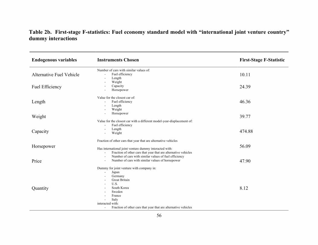
56

Table 2b. First-stage F-statistics: Fuel economy standard model with “international joint venture country” dummy interactions

Endogenous variables Instruments Chosen First-Stage F-Statistic

Alternative Fuel Vehicle Number of cars with similar values of:

- Fuel efficiency - Length - Weight - Capacity - Horsepower

Value for the closest car of:

- Fuel efficiency - Length - Weight - Horsepower

Value for the closest car with a different model-year-displacement of:

- Fuel efficiency - Length - Weight

Fraction of other cars that year that are alternative vehicles Has international joint venture dummy interacted with:

- Fraction of other cars that year that are alternative vehicles - Number of cars with similar values of fuel efficiency - Number of cars with similar values of horsepower

Dummy for joint venture with company in:

- Japan - Germany - Great Britain - U.S. - South Korea - Sweden - France - Italy

interacted with: - Fraction of other cars that year that are alternative vehicles

10.11

Fuel Efficiency 24.39

Length 46.36

Weight 39.77

Capacity 474.88

Horsepower 56.09

Price 47.90

Quantity 8.12

57

- Number of cars with similar values of fuel efficiency - Number of cars with similar values of horsepower

Difference between fuel economy target and the number of cars with similar values of fuel efficiency Different between Corporate Average Fuel Consumption (CAFC) target and the number of cars with similar values of fuel efficiency, interacted with dummy for being required to meet CAFC target

58

Table 3. Results of structural econometric model of supply and demand, 2010-2013

(1) (2) (3) Mean ! of marginal utility of: Alternative vehicle (dummy) 0.210***

(0.006) 0.106*** (0.001)

0.106*** (0.012)

Fuel efficiency (100km/L) 0.211*** (0.007)

0.235*** (0.002)

0.235*** (0.003)

Length (m) 0.017*** (0.002)

0.294*** (0.004)

0.294*** (0.006)

Weight (metric ton) 0.220*** (0.001)

0.281*** (0.001)

0.281*** (0.002)

Capacity (number of seats) 0.005*** (0.001)

-0.133*** (0.002)

-0.133*** (0.004)

Horsepower (PS) 0.070*** (0.003)

0.168*** (0.005)

0.168*** (0.009)

Constant 0.118*** (0.003)

0.333*** (0.000)

0.333*** (0.003)

Standard deviation " of marginal utility of: Alternative vehicle (dummy) 0.107***

(0.006) 0.163*** (0.003)

0.163*** (0.002)

Fuel efficiency (100km/L) 0.133*** (0.000)

0.112*** (0.001)

0.112*** (0.004)

Length (m) 0.078*** (0.004)

-0.009 (0.007)

-0.009** (0.003)

Weight (metric ton) 0.187*** (0.002)

0.347*** (0.004)

0.347*** (0.005)

Capacity (number of seats) 0.065*** (0.002)

0.105*** (0.000)

0.105*** (0.007)

Horsepower (0.01PS) 0.046*** (0.007)

0.029*** (0.001)

0.029*** (0.008)

Constant 0.207*** (0.001)

0.210*** (0.002)

0.210*** (0.004)

Parameter # in marginal disutility of price (1,000 Yuan) 0.348***

(0.001) 0.420*** (0.000)

0.420*** (0.000)

59

Coefficient $ in marginal cost on: Alternative vehicle (dummy) 0.241***

(0.008) 0.139*** (0.003)

0.139*** (0.002)

Fuel efficiency (100km/L) 0.093*** (0.007)

0.060*** (0.000)

0.060*** (0.005)

Length (m) 0.113*** (0.004)

0.126*** (0.003)

0.126*** (0.010)

Weight (metric ton) 0.121*** (0.005)

0.101*** (0.003)

0.101*** (0.004)

Capacity (number of seats) 0.230*** (0.006)

0.156*** (0.002)

0.156*** (0.003)

Horsepower (0.01PS) 0.157*** (0.003)

0.113*** (0.003)

0.113*** (0.010)

State-owned (dummy) 0.177*** (0.002)

0.111*** (0.005)

0.111*** (0.002)

Constant 0.191*** (0.002)

0.245*** (0.006)

0.245*** (0.003)

Coefficient % on quantity in marginal cost 0.014***

(0.001) 0.007*** (0.000)

0.007*** (0.001)

Coefficient & in marginal cost on joint venture with: Mazda 0.105***

(0.005) 0.158*** (0.000)

0.158*** (0.003)

Honda -0.085*** (0.002)

-0.064*** (0.006)

-0.064*** (0.003)

Kaihatsu 0.181*** (0.003)

0.054*** (0.004)

0.054*** (0.001)

Toyota 0.134*** (0.001)

0.219*** (0.004)

0.219*** (0.007)

Suzuki 0.012*** (0.001)

-0.028*** (0.005)

-0.028** (0.010)

Nissan 0.029*** (0.001)

0.033*** (0.000)

0.033*** (0.002)

Mitsubishi 0.012*** (0.001)

0.185*** (0.000)

0.185*** (0.001)

60

Isuzu -0.092*** (0.003)

-0.110*** (0.007)

-0.110*** (0.007)

Daimler -0.237*** (0.003)

-0.224*** (0.002)

-0.224*** (0.003)

BMW -0.081*** (0.004)

-0.059*** (0.001)

-0.059*** (0.004)

Volkswagen 0.033*** (0.001)

0.035*** (0.000)

0.035*** (0.006)

Audi 0.151*** (0.004)

0.092*** (0.007)

0.092*** (0.004)

Lotus -0.245*** (0.002)

-0.253*** (0.004)

-0.253*** (0.005)

GM -0.225*** (0.001)

-0.189*** (0.005)

-0.189*** (0.006)

Ford -0.051*** (0.010)

0.029*** (0.003)

0.029*** (0.005)

Chrysler -0.037*** (0.008)

-0.135*** (0.006)

-0.135*** (0.005)

Hyundai -0.024*** (0.001)

0.003 (0.008)

0.003 (0.006)

Kia -0.159*** (0.004)

-0.115*** (0.001)

-0.115*** (0.011)

Volvo 0.025*** (0.001)

0.134*** (0.001)

0.134*** (0.005)

Saab 0.122*** (0.001)

0.193*** (0.001)

0.193*** (0.005)

PSA -0.219*** (0.001)

-0.31*** (0.001)

-0.31*** (0.000)

Fiat -0.149*** (0.006)

-0.382*** (0.000)

-0.382*** (0.004)

Coefficient in marginal cost on international joint venture-technology interactions: Has international joint venture * alternative vehicle -0.070***

�0.000� 0.144*** (0.001)

0.144*** (0.008)

Has international joint venture * fuel efficiency -0.230*** (0.000)

-0.160*** (0.005)

-0.160*** (0.005)

61

Has international joint venture * horsepower -0.170*** (0.000)

-0.073*** (0.003)

-0.073*** (0.008)

Coefficient in marginal cost on having international joint venture with a particular country interacted with technology:

Japan * alternative vehicle -0.420***

(0.003) -0.420***

(0.003) Japan * fuel efficiency -0.713***

(0.003) -0.713***

(0.004) Japan * horsepower -0.851***

(0.002) -0.851***

(0.004) Germany * alternative vehicle 0.118***

(0.001) 0.118*** (0.005)

Germany * fuel efficiency 0.708*** (0.002)

0.708*** (0.003)

Germany * horsepower 0.774*** (0.005)

0.774*** (0.001)

Britain * alternative vehicle 1.005***

(0.002) 1.005*** (0.004)

Britain * fuel efficiency 0.213*** (0.003)

0.213*** (0.004)

Britain * horsepower 0.615*** (0.003)

0.615*** (0.003)

US * alternative vehicle -0.203***

(0.002) -0.203***

(0.004) US * fuel efficiency -0.149***

(0.009) -0.149***

(0.004) US * horsepower -0.662***

(0.002) -0.662***

(0.002) South Korea * alternative vehicle 0.445***

(0.002) 0.445*** (0.002)

62

South Korea * fuel efficiency 0.678*** (0.002)

0.678*** (0.004)

South Korea * horsepower 0.361*** (0.001)

0.361*** (0.010)

Sweden * alternative vehicle 0.981***

(0.004) 0.981*** (0.004)

Sweden * fuel efficiency 0.748*** (0.002)

0.748*** (0.004)

Sweden * horsepower 0.912*** (0.001)

0.912*** (0.001)

France * alternative vehicle 0.268***

(0.010) 0.268*** (0.007)

France * fuel efficiency 0.437*** (0.002)

0.437*** (0.007)

France * horsepower 0.203*** (0.000)

0.203*** (0.003)

Italy * alternative vehicle 0.098***

(0.002) 0.098*** (0.002)

Italy * fuel efficiency 0.336*** (0.002)

0.336*** (0.003)

Italy * horsepower 1.042*** (0.000)

1.042*** (0.004)

Coefficient in marginal cost on having international joint venture with a particular car company from Japan or US interacted with technology:

Mazda * fuel efficiency -0.182***

(0.006) Mazda * horsepower -0.264***

(0.003) Mazda * alternative vehicle -0.146***

(0.004)

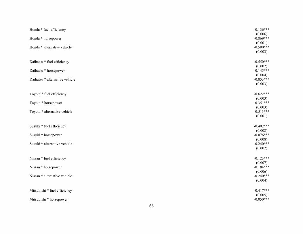
63

Honda * fuel efficiency -0.136*** (0.006)

Honda * horsepower -0.869*** (0.001)

Honda * alternative vehicle -0.580*** (0.003)

Daihatsu * fuel efficiency -0.550***

(0.002) Daihatsu * horsepower -0.145***

(0.004) Daihatsu * alternative vehicle -0.853***

(0.003) Toyota * fuel efficiency -0.622***

(0.003) Toyota * horsepower -0.351***

(0.003) Toyota * alternative vehicle -0.513***

(0.001) Suzuki * fuel efficiency -0.402***

(0.008) Suzuki * horsepower -0.076***

(0.008) Suzuki * alternative vehicle -0.240***

(0.002) Nissan * fuel efficiency -0.123***

(0.007) Nissan * horsepower -0.184***

(0.006) Nissan * alternative vehicle -0.240***

(0.004) Mitsubishi * fuel efficiency -0.417***

(0.005) Mitsubishi * horsepower -0.050***

64

(0.009) Mitsubishi * alternative vehicle -0.903***

(0.002) Isuzu * fuel efficiency -0.945***

(0.007) Isuzu * horsepower -0.491***

(0.004) Isuzu * alternative vehicle -0.489***

(0.003) GM * fuel efficiency -0.338***

(0.008) GM * horsepower -0.900***

(0.003) GM * alternative vehicle -0.369***

(0.001) Ford * fuel efficiency -0.111***

(0.005) Ford * horsepower -0.780***

(0.006) Ford * alternative vehicle -0.390***

(0.003) Chrysler * fuel efficiency -0.242***

(0.003) Chrysler * horsepower -0.404***

(0.005) Chrysler * alternative vehicle -0.096***

(0.005)

Coefficient in marginal cost on fuel economy policy variables: Difference between fuel economy target and actual fuel efficiency (100km/L) 0.547***

(0.000) 0.547*** (0.004)

0.547*** (0.007)

Firm needs to meet Corporate Average Fuel Consumption (CAFC) target (dummy) 0.279*** 0.279*** 0.279***

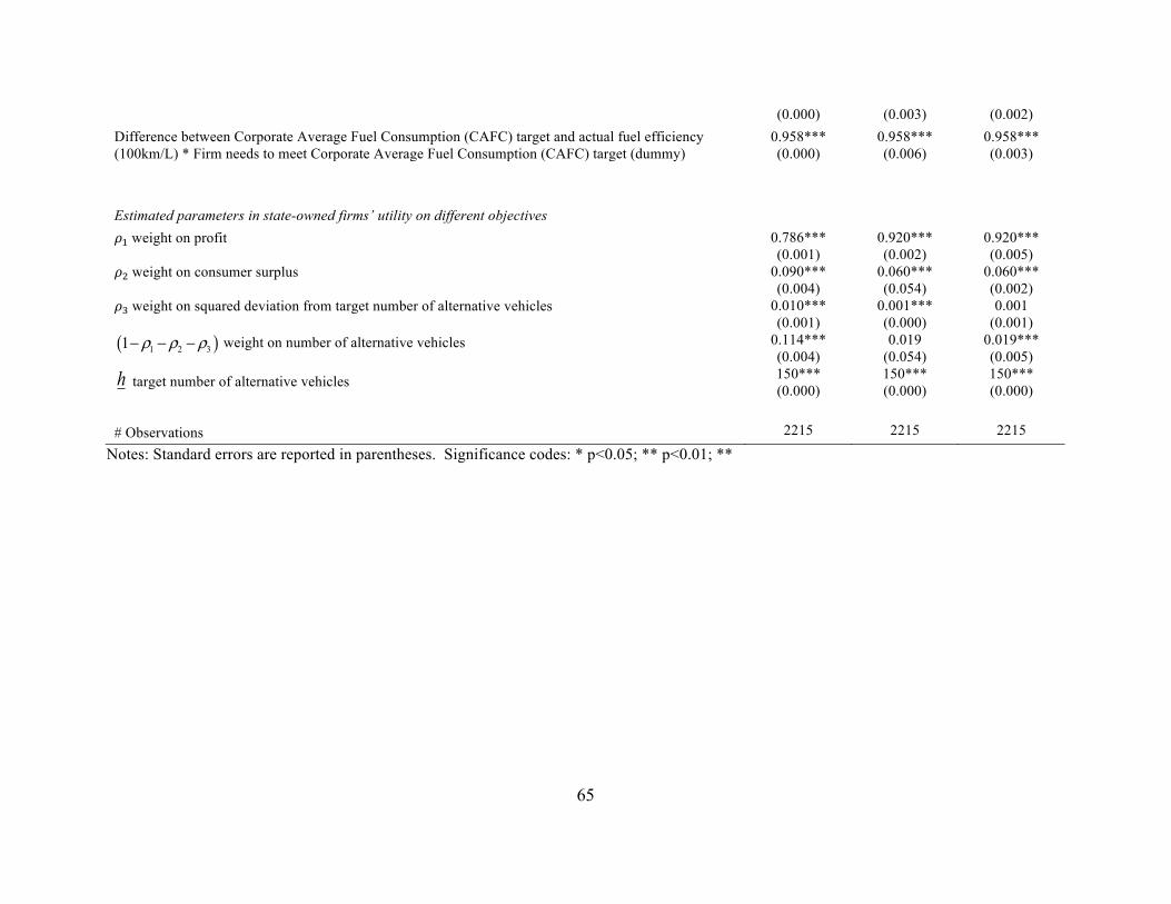
65

(0.000) (0.003) (0.002) Difference between Corporate Average Fuel Consumption (CAFC) target and actual fuel efficiency (100km/L) * Firm needs to meet Corporate Average Fuel Consumption (CAFC) target (dummy)

0.958*** (0.000)

0.958*** (0.006)

0.958*** (0.003)

Estimated parameters in state-owned firms’ utility on different objectives '(weight on profit 0.786***

(0.001) 0.920*** (0.002)

0.920*** (0.005)

'*weight on consumer surplus 0.090*** (0.004)

0.060*** (0.054)

0.060*** (0.002)

'+weight on squared deviation from target number of alternative vehicles 0.010*** (0.001)

0.001*** (0.000)

0.001 (0.001)

( )1 2 31 ρ ρ ρ− − − weight on number of alternative vehicles 0.114*** (0.004)

0.019 (0.054)

0.019*** (0.005)

h target number of alternative vehicles 150*** (0.000)

150*** (0.000)

150*** (0.000)

# Observations 2215 2215 2215

Notes: Standard errors are reported in parentheses. Significance codes: * p<0.05; ** p<0.01; **

66

Table 4: Net effects of forming joint ventures with each U.S. and Japan car company on the marginal cost of the technology-related vehicle characteristics Alternative Vehicle Fuel Efficiency Horsepower Japanese firms Mazda -0.422***

(0.009) -1.055***

(0.009) -1.188***

(0.010) Honda -0.856***

(0.009) -1.009***

(0.009) -1.793***

(0.009) Daihatsu -1.129***

(0.009) -1.423***

(0.007) -1.069***

(0.009) Toyota -0.789***

(0.009) -1.495***

(0.007) -1.275***

(0.009) Suzuki -0.516***

(0.009) -1.275***

(0.010) -1.000***

(0.012) Nissan -0.460***

(0.009) -0.996***

(0.009) -1.108***

(0.011) Mitsubishi -1.179***

(0.009) -1.290***

(0.008) -1.108***

(0.013) Isuzu -0.765***

(0.009) -1.818***

(0.009) -1.415***

(0.010) US firms GM -0.428***

(0.009) -0.647***

(0.010) -1.635***

(0.009) Ford -0.449***

(0.009) -0.420***

(0.008) -1.515***

(0.011) Chrysler -0.155***

(0.010) -0.551***

(0.007) -1.139***

(0.010) Notes: Standard errors are reported in parentheses. Significance codes: * p<0.05; ** p<0.01; *** p<0.001

67

Table 5. Welfare 2010 2011 2012 2013 Consumer surplus (1,000 Yuan) 13,916.00*** 7,203.50*** 818.77*** 2,631.90*** (591.99) (255.83) (40.37) (107.12) Total firm profit for private firms 862.82*** 613.69*** 787.00*** 1,944.60*** (0.14) (0.09) (0.77) (0.22) Average firm profit for private firms 86.28*** 61.37*** 87.45*** 216.07*** (0.01) (0.01) (0.01) (0.03) Total firm utility for state-owned firms 1,993.10*** 2,902.40*** 3,036.40*** 4,156.60*** (5.47) (7.90) (8.08) (11.22) Average firm utility for state-owned firms 76.66*** 100.08*** 97.95*** 115.46*** (0.21) (0.27) (0.26) (0.31)

Notes: Welfare is calculated using parameter estimates from Specification (2) of Table 3. Consumer surplus is in 1,000 Yuan; all other values are in units of billion Yuan. Standard errors are reported in parentheses. Significance codes: * p<0.05; ** p<0.01; ***p<0.001

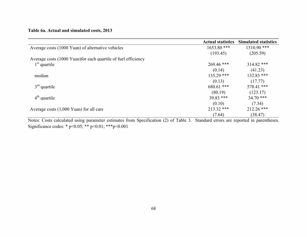
68

Table 6a. Actual and simulated costs, 2013

Actual statistics Simulated statistics Average costs (1000 Yuan) of alternative vehicles 1653.80 *** 1510.90 *** (193.45) (205.59) Average costs (1000 Yuan)for each quartile of fuel efficiency 1st quartile 269.46 *** 314.82 *** (0.14) (41.23) median 135.29 *** 132.83 *** (0.13) (17.77) 3rd quartile 680.61 *** 578.41 *** (80.19) (123.17) 4th quartile 39.83 *** 34.70 *** (0.10) (7.34) Average costs (1,000 Yuan) for all cars 213.32 *** 212.26 *** (7.64) (38.47)

Notes: Costs calculated using parameter estimates from Specification (2) of Table 3. Standard errors are reported in parentheses. Significance codes: * p<0.05; ** p<0.01; ***p<0.001

69

Table 6b. Actual and simulated welfare, 2013 Actual Simulated Consumer surplus (1000 Yuan) 2631.90*** 2402.80*** (107.12) (236.57) Total firm profit for private firms 1944.60*** 2119.10*** (0.22) (189.05) Average firm profit for private firms 216.07*** 235.46*** (0.03) (21.01) Total firm utility for state-owned firms 4156.60*** 4159.60*** (11.22) (589.79) Average firm utility for state-owned firms 115.46*** 115.54*** (0.31) (16.38)

Notes: Welfare is calculated using parameter estimates from Specification (2) of Table 3. Consumer surplus is in 1,000 Yuan; all other values are in units of billion Yuan. Standard errors are reported in parentheses. Significance codes: * p<0.05; ** p<0.01; ***p<0.001

70

Table 7a: Own price elasticities for state-owned models

Model displacement (1) (2) Focus 1.8L -44.347 -52.666 C-Quatre 1.6L -50.225 -50.341 Eado 1.6L -34.757 -38.229 Gran Lavida 1.6L -58.593 -75.436 Jetta 1.6L -35.135 -40.909 Buick Excellegt 1.5L -41.243 -46.862 Bora 1.6L -46.717 -52.098 Langdong 1.6L -53.845 -66.084 Verna 1.4L -35.068 -39.212 Cruz 1.6L -55.975 -63.260 Corolla Ex 1.6L -39.423 -44.728 Corolla -57.530 -58.988 Octavia 1.6L -54.133 -60.071 Lotus L5 -48.211 -54.566 H6 1.5T -46.692 -52.277 Honda CR-V 2.4L -98.997 -118.980 Tiguan 1.8T -86.887 -99.631 ix35 2.0L -71.108 -81.194 Touran 1.4T -63.464 -72.159 Succe1.5L -27.606 -30.919

Note: Specifications (1) and (2) correspond to Specifications (1) and (2) in Table 3.

71

Table 7b: Cross price elasticities for state-owned model

Model displacement (1) (2) Focus 1.8L 0.000 0.000 C-Quatre 1.6L 0.000 0.000 Eado 1.6L 0.000 0.000 Gran Lavida 1.6L 0.000 0.000 Jetta 1.6L 0.000 0.000 Buick Excellegt 1.5L 0.000 0.000 Bora 1.6L 0.000 0.000 Langdong 1.6L 0.000 0.000 Verna 1.4L 0.000 0.000 Cruz 1.6L 0.000 0.000 Corolla Ex 1.6L 0.000 0.000 Corolla 0.000 0.000 Octavia 1.6L 0.000 0.000 Lotus L5 0.000 0.000 H6 1.5T 0.000 0.000 Honda CR-V 2.4L 0.000 0.000 Tiguan 1.8T 0.000 0.000 ix35 2.0L 0.000 0.000 Touran 1.4T 0.000 0.000 Succe1.5L 0.000 0.000

Notes: The hybrid vehicle picked here is "Buick E-assist 2.4L hybrid". Specifications (1) and (2) correspond to Specifications (1) and (2) in Table 3.

72

Table 8a. New car simulation 1: New car is like “Buick E-assist 2.4L hybrid" but with fuel efficiency 1.25 times more efficient Simulated

statistics Difference from

base case Total market share for all alternative vehicles 0.001207

(0.042711) 0.000017

(0.004271) Market share for each quartile of fuel efficiency

1st quartile 0.042203*** (0.004093)

-0.001531** (0.000460)

median 0.011085*** (0.001049)

0.000074 (0.000107)

3rd quartile 0.073918*** (0.007033)

0.000051 (0.000712)

4th quartile 0.001050*** (0.000100)

-0.000014 (0.000011)

Average costs of alternative vehicles 1578.76 (10351.70)

95.50 (1035.41)

Average costs for each quartile of fuel efficiency 1st quartile 311.40***

(33.50) 16.10** (5.55)

median 129.61*** (13.44)

14.66*** (2.31)

3rd quartile 563.19*** (111.46)

48.39** (16.74)

4th quartile 32.63*** (5.99)

5.67*** (0.98)

Average costs for all cars 208.09 (409.74)

33.22 (41.17)

Consumer surplus (1000 Yuan) 2446.06 (59461669.03)

-9.70 (5950000.00)

Total firm profit for private firms 2019.43*** (146.34)

51.40* (24.94)

Average firm profit for private firms 224.38*** (16.26)

5.71* (2.77)

Total firm utility for state-owned firms 4074.54 (33308113.46)

296.10 (3330000.00)

Average firm utility for state-owned firms 113.18 (925225.37)

8.22 (92500.00)

The utility of the firm producing the new car 388.49 (33308033.22)

15.12 (3330000.00)

Notes: Costs and consumer surplus are in 1,000 Yuan. Profit, and firm utility are in billion Yuan. Standard errors are reported in parentheses. Significance stars following the difference from base case indicated the significance of a two-sample t-test of the difference between the statistic in the counterfactual simulation and that in the base-case simulation. Significance codes: * p<0.05; ** p<0.01; ***p<0.001

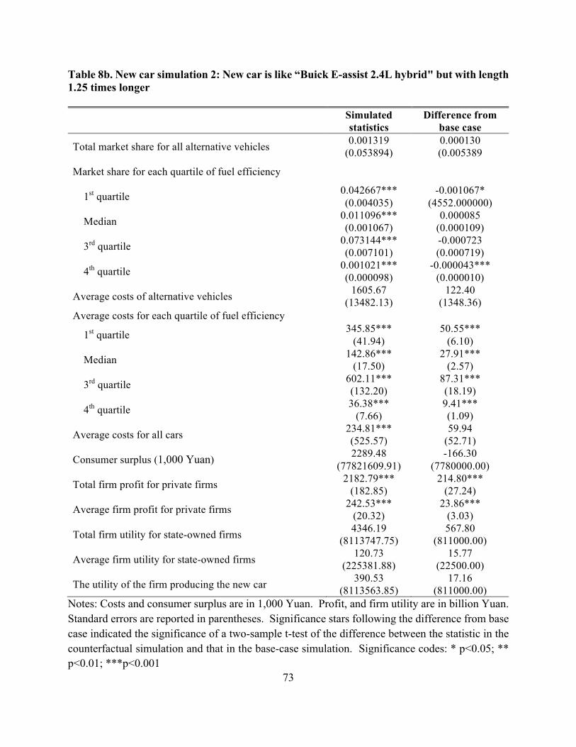
73

Table 8b. New car simulation 2: New car is like “Buick E-assist 2.4L hybrid" but with length 1.25 times longer

Simulated statistics

Difference from base case

Total market share for all alternative vehicles 0.001319 (0.053894)

0.000130 (0.005389

Market share for each quartile of fuel efficiency

1st quartile 0.042667*** (0.004035)

-0.001067* (4552.000000)

Median 0.011096*** (0.001067)

0.000085 (0.000109)

3rd quartile 0.073144*** (0.007101)

-0.000723 (0.000719)

4th quartile 0.001021*** (0.000098)

-0.000043*** (0.000010)

Average costs of alternative vehicles 1605.67 (13482.13)

122.40 (1348.36)

Average costs for each quartile of fuel efficiency

1st quartile 345.85*** (41.94)

50.55*** (6.10)

Median 142.86*** (17.50)

27.91*** (2.57)

3rd quartile 602.11*** (132.20)

87.31*** (18.19)

4th quartile 36.38*** (7.66)

9.41*** (1.09)

Average costs for all cars 234.81*** (525.57)

59.94 (52.71)

Consumer surplus (1,000 Yuan) 2289.48 (77821609.91)

-166.30 (7780000.00)

Total firm profit for private firms 2182.79*** (182.85)

214.80*** (27.24)

Average firm profit for private firms 242.53*** (20.32)

23.86*** (3.03)

Total firm utility for state-owned firms 4346.19 (8113747.75)

567.80 (811000.00)

Average firm utility for state-owned firms 120.73 (225381.88)

15.77 (22500.00)

The utility of the firm producing the new car 390.53 (8113563.85)

17.16 (811000.00)

Notes: Costs and consumer surplus are in 1,000 Yuan. Profit, and firm utility are in billion Yuan. Standard errors are reported in parentheses. Significance stars following the difference from base case indicated the significance of a two-sample t-test of the difference between the statistic in the counterfactual simulation and that in the base-case simulation. Significance codes: * p<0.05; ** p<0.01; ***p<0.001

74

Table 8c. New car simulation 3: New car is like “Buick E-assist 2.4L hybrid" but with weight 1.25 times heavier

Simulated statistics

Difference from base case

Total market share for all alternative vehicles 0.001377 (0.048249)

0.000187 (0.004825)

Market share for each quartile of fuel efficiency

1st quartile 0.041540*** (0.004001)

-0.002194*** (0.000452)

Median 0.010992*** (0.001063)

-0.000019 (0.000109)

3rd quartile 0.072944*** (0.006961)

-0.000923 (0.000705)

4th quartile 0.001032*** (0.000098)

-0.000032* (0.000010)

Average costs of alternative vehicles 1619.51 (12259.81)

136.20 (1226.17)

Average costs for each quartile of fuel efficiency

1st quartile 346.80*** (37.11)

51.50*** (5.78)

Median 146.82*** (15.45)

31.87*** (2.43)

3rd quartile 620.85*** (121.24)

106.05*** (17.41)

4th quartile 40.38*** (6.72)

13.41*** (1.02)

Average costs for all cars 246.88 (480.46)

72.01 (48.22)

Consumer surplus (1,000 Yuan) 2390.61 (68208985.62)

-65.20 (6820000.00)

Total firm profit for private firms 2267.29*** (158.17)

299.30*** (25.65)

Average firm profit for private firms 251.92*** (17.57)

33.25*** (2.85)

Total firm utility for state-owned firms 4473.21 (16417294.51)

694.80 (1640000.00)

Average firm utility for state-owned firms 124.26 (456035.96)

19.30 (45600.00)

The utility of the firm producing the new car 402.31 (16417140.45)

28.94 (1640000.00)

Notes: Costs and consumer surplus are in 1,000 Yuan. Profit, and firm utility are in billion Yuan. Standard errors are reported in parentheses. Significance stars following the difference from base case indicated the significance of a two-sample t-test of the difference between the statistic in the counterfactual simulation and that in the base-case simulation. Significance codes: * p<0.05; ** p<0.01; ***p<0.001

75

Table 8d. New car simulation 4: New car is like “Buick E-assist 2.4L hybrid" but with weight 1.25 times lighter

Simulated statistics

Difference from base case

Total market share for all alternative vehicles 0.001279 (0.039759)

0.000089 (0.003976)

Market share for each quartile of fuel efficiency

1st quartile 0.044954*** (0.003995)

0.001220** (0.000452)

median 0.010973*** (0.001029)

-0.000038 (0.000105)

3rd quartile 0.072894*** (0.006914)

-0.000973 (0.000700)

4th quartile 0.001030*** (0.000098)

-0.000034** (0.000010)

Average costs of alternative vehicles 1595.88 (9373.03)

112.60 (937.53)

Average costs for each quartile of fuel efficiency

1st quartile 358.49 (33.86)

63.19*** (5.57)

median 135.69 (13.34)

20.74*** (2.31)

3rd quartile 582.18 (108.86)

67.38*** (16.57)

4th quartile 34.78 (6.14)

7.81*** (0.99)

Average costs for all cars 224.59 (367.93)

49.72 (37.02)

Consumer surplus (1,000 Yuan) 2467.58 (54839246.43)

11.80 (5480000.00)

Total firm profit for private firms 2205.67*** (151.67)

237.70*** (25.25)

Average firm profit for private firms 245.07*** (16.85)

26.40*** (2.81)

Total firm utility for state-owned firms 4235.65 (36851485.26)

457.20 (3690000.00)

Average firm utility for state-owned firms 117.66 (1023652.37)

12.70 (102000.00)

The utility of the firm producing the new car 393.52 (36851425.50)

20.15 (3690000.00)

Notes: Costs and consumer surplus are in 1,000 Yuan. Profit, and firm utility are in billion Yuan. Standard errors are reported in parentheses. Significance stars following the difference from base case indicated the significance of a two-sample t-test of the difference between the statistic in the counterfactual simulation and that in the base-case simulation. Significance codes: * p<0.05; ** p<0.01; ***p<0.001

76

Table 8e. New car simulation 5: New car is like “Buick E-assist 2.4L hybrid" but with one more seat

Simulated statistics

Difference from base case

Total market share for all alternative vehicles 0.001362 (0.040752)

0.000172 (0.004075)

Market share for each quartile of fuel efficiency

1st quartile 0.040783*** (0.004049)

-0.002951*** (0.000456)

median 0.010788*** (0.001050)

-0.000223* (0.000107)

3rd quartile 0.072859*** (0.007034)

-0.001008 (0.000712)

4th quartile 0.001041*** (0.000099)

-0.000023* (0.000011)

Average costs of alternative vehicles 1615.79 (9565.90)

132.50 (956.81)

Average costs for each quartile of fuel efficiency

1st quartile 316.26*** (33.48)

20.96** (5.55)

median 133.12*** (13.05)

18.17*** (2.29)

3rd quartile 584.39*** (108.55)

69.59*** (16.55)

4th quartile 36.23*** (5.82)

9.26*** (0.97)

Average costs for all cars 226.08 (377.49)

51.21 (37.97)

Consumer surplus (1,000 Yuan) 2339.95 (56796217.24)

-115.80 (5680000.00)

Total firm profit for private firms 2147.57*** (149.65)

179.60*** (25.13)

Average firm profit for private firms 238.62*** (16.63)

19.95*** (2.79)

Total firm utility for state-owned firms 4255.47 (38231291.98)

477.10 (3820000.00)

Average firm utility for state-owned firms 118.21 (1061980.33)

13.25 (106000.00)

The utility of the firm producing the new car 387.23 (38231231.49)

13.86 (3820000.00)

Notes: Costs and consumer surplus are in 1,000 Yuan. Profit, and firm utility are in billion Yuan. Standard errors are reported in parentheses. Significance stars following the difference from base case indicated the significance of a two-sample t-test of the difference between the statistic in the counterfactual simulation and that in the base-case simulation. Significance codes: * p<0.05; ** p<0.01; ***p<0.001

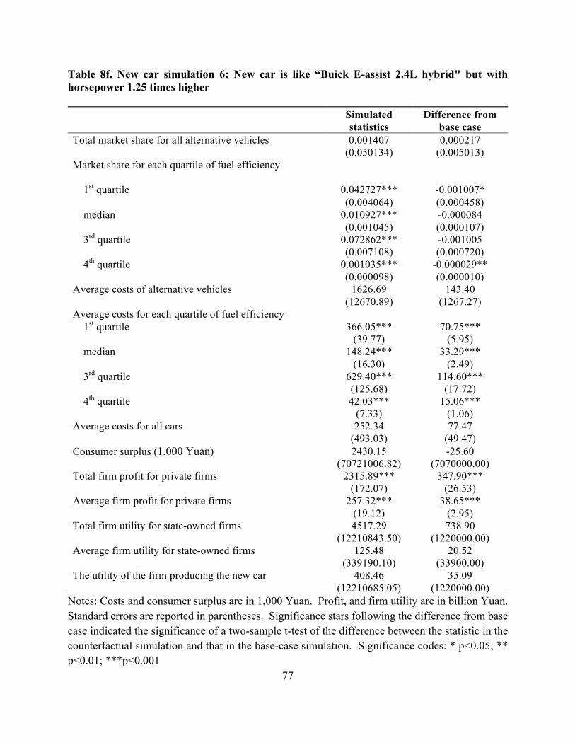
77

Table 8f. New car simulation 6: New car is like “Buick E-assist 2.4L hybrid" but with horsepower 1.25 times higher Simulated

statistics Difference from

base case Total market share for all alternative vehicles 0.001407

(0.050134) 0.000217

(0.005013) Market share for each quartile of fuel efficiency

1st quartile 0.042727*** (0.004064)

-0.001007* (0.000458)

median 0.010927*** (0.001045)

-0.000084 (0.000107)

3rd quartile 0.072862*** (0.007108)

-0.001005 (0.000720)

4th quartile 0.001035*** (0.000098)

-0.000029** (0.000010)

Average costs of alternative vehicles 1626.69 (12670.89)

143.40 (1267.27)

Average costs for each quartile of fuel efficiency 1st quartile 366.05***

(39.77) 70.75***

(5.95) median 148.24***

(16.30) 33.29***

(2.49) 3rd quartile 629.40***

(125.68) 114.60***

(17.72) 4th quartile 42.03***

(7.33) 15.06***

(1.06) Average costs for all cars 252.34

(493.03) 77.47

(49.47) Consumer surplus (1,000 Yuan) 2430.15

(70721006.82) -25.60

(7070000.00) Total firm profit for private firms 2315.89***

(172.07) 347.90***

(26.53) Average firm profit for private firms 257.32***

(19.12) 38.65***

(2.95) Total firm utility for state-owned firms 4517.29

(12210843.50) 738.90

(1220000.00)

Average firm utility for state-owned firms 125.48 (339190.10)

20.52 (33900.00)

The utility of the firm producing the new car 408.46 (12210685.05)

35.09 (1220000.00)

Notes: Costs and consumer surplus are in 1,000 Yuan. Profit, and firm utility are in billion Yuan. Standard errors are reported in parentheses. Significance stars following the difference from base case indicated the significance of a two-sample t-test of the difference between the statistic in the counterfactual simulation and that in the base-case simulation. Significance codes: * p<0.05; ** p<0.01; ***p<0.001

78

Table 8g. New car simulation 7: New car is like “Buick E-assist 2.4L hybrid" but with horsepower 1.25 times lower Simulated

statistics Difference from

base case Total market share for all alternative vehicles 0.001287

(0.040607) 0.000097

(0.004061) Market share for each quartile of fuel efficiency

1st quartile 0.040054*** (0.003911)

-0.003680*** (0.000444)

median 0.011042*** (0.001062)

0.000031 (0.000108)

3rd quartile 0.074226*** (0.006981)

0.000359 (0.000707)

4th quartile 0.001035*** (0.000099)

-0.000029** (0.000011)

Average costs of alternative vehicles 1597.97 (9308.00)

114.70 (931.03)

Average costs for each quartile of fuel efficiency 1st quartile 311.36***

(33.40) 16.06** (5.54)

median 138.93*** (13.95)

23.98*** (2.34)

3rd quartile 602.02*** (110.81)

87.22*** (16.70)

4th quartile 36.30*** (6.14)

9.33*** (0.99)

Average costs for all cars 228.75 (367.18)

53.88 (36.94)

Consumer surplus (1,000 Yuan) 2581.09 (53645483.33)

125.30 (5360000.00)

Total firm profit for private firms 2124.26*** (149.70)

156.30*** (25.14)

Average firm profit for private firms 236.03*** (16.63)

17.36*** (2.79)

Total firm utility for state-owned firms 4293.66 (34671505.89)

515.30 (3470000.00)

Average firm utility for state-owned firms 119.27 (963097.39)

14.31 (96300.00)

The utility of the firm producing the new car 405.26 (34671426.21)

31.89 (3470000.00)

Notes: Costs and consumer surplus are in 1,000 Yuan. Profit, and firm utility are in billion Yuan. Standard errors are reported in parentheses. Significance stars following the difference from base case indicated the significance of a two-sample t-test of the difference between the statistic in the counterfactual simulation and that in the base-case simulation. Significance codes: * p<0.05; ** p<0.01; ***p<0.001

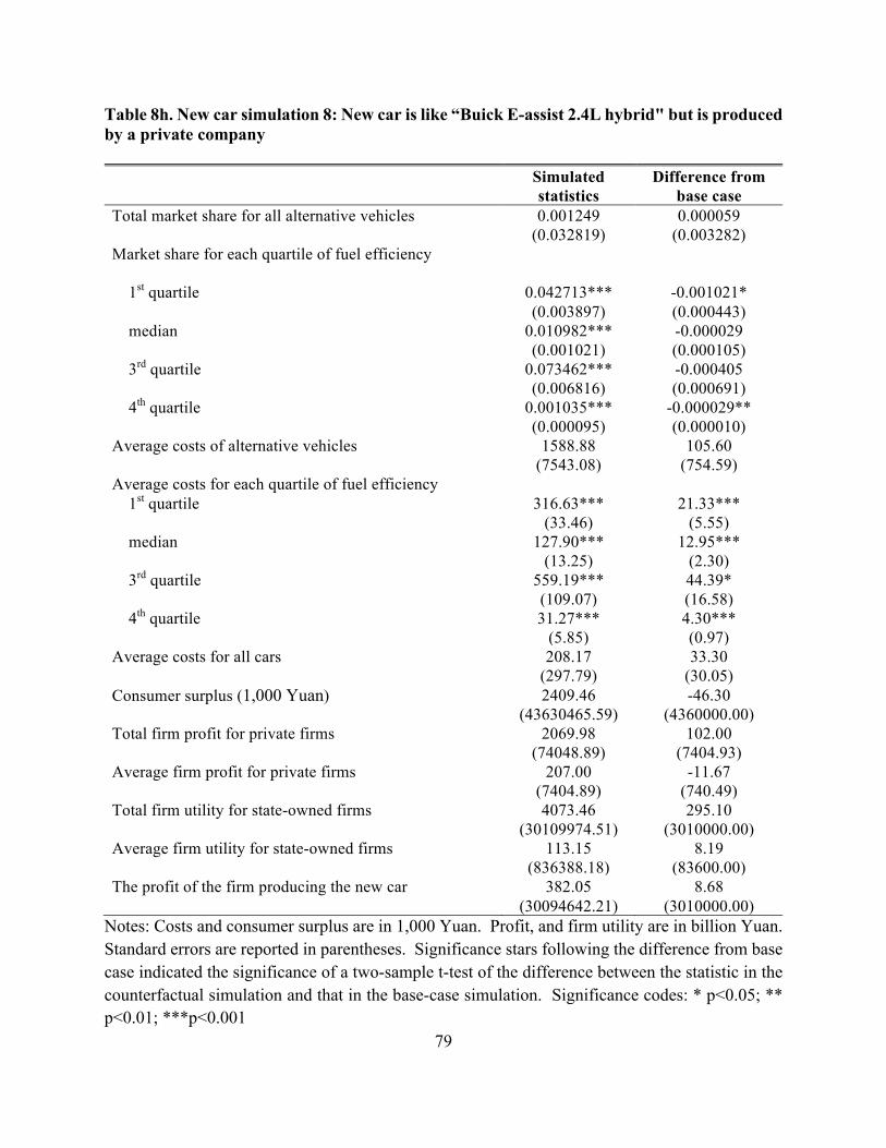
79

Table 8h. New car simulation 8: New car is like “Buick E-assist 2.4L hybrid" but is produced by a private company Simulated

statistics Difference from

base case Total market share for all alternative vehicles 0.001249

(0.032819) 0.000059

(0.003282) Market share for each quartile of fuel efficiency

1st quartile 0.042713*** (0.003897)

-0.001021* (0.000443)

median 0.010982*** (0.001021)

-0.000029 (0.000105)

3rd quartile 0.073462*** (0.006816)

-0.000405 (0.000691)

4th quartile 0.001035*** (0.000095)

-0.000029** (0.000010)

Average costs of alternative vehicles 1588.88 (7543.08)

105.60 (754.59)

Average costs for each quartile of fuel efficiency 1st quartile 316.63***

(33.46) 21.33***

(5.55) median 127.90***

(13.25) 12.95***

(2.30) 3rd quartile 559.19***

(109.07) 44.39* (16.58)

4th quartile 31.27*** (5.85)

4.30*** (0.97)

Average costs for all cars 208.17 (297.79)

33.30 (30.05)

Consumer surplus (1,000 Yuan) 2409.46 (43630465.59)

-46.30 (4360000.00)

Total firm profit for private firms 2069.98 (74048.89)

102.00 (7404.93)

Average firm profit for private firms 207.00 (7404.89)

-11.67 (740.49)

Total firm utility for state-owned firms 4073.46 (30109974.51)

295.10 (3010000.00)

Average firm utility for state-owned firms 113.15 (836388.18)

8.19 (83600.00)

The profit of the firm producing the new car 382.05 (30094642.21)

8.68 (3010000.00)

Notes: Costs and consumer surplus are in 1,000 Yuan. Profit, and firm utility are in billion Yuan. Standard errors are reported in parentheses. Significance stars following the difference from base case indicated the significance of a two-sample t-test of the difference between the statistic in the counterfactual simulation and that in the base-case simulation. Significance codes: * p<0.05; ** p<0.01; ***p<0.001

80

Table 8i. New car simulation 9: New car is like “Buick E-assist 2.4L hybrid" but firm does not form a joint venture with any international companies Simulated

statistics Difference from

base case Total market share for all alternative vehicles 0.001234

(0.031783) 0.000044

(0.003178) Market share for each quartile of fuel efficiency

1st quartile 0.043777*** (0.003902)

0.000043 (0.000444)

median 0.010901*** (0.001022)

-0.000110 (0.000105)

3rd quartile 0.073801*** (0.006815)

-0.000066 (0.000691)

4th quartile 0.001034*** (0.000095)

-0.000030** (0.000010)

Average costs of alternative vehicles 1585.19 (7340.63)

101.90 (734.35)

Average costs for each quartile of fuel efficiency 1st quartile 331.39***

(34.93) 36.09***

(5.64) median 128.21***

(13.83) 13.26***

(2.33) 3rd quartile 568.38***

(109.79) 53.58** (16.63)

4th quartile 32.07*** (6.10)

5.10*** (0.98)

Average costs for all cars 211.70 (288.77)

36.83 (29.16)

Consumer surplus (1,000 Yuan) 2599.37 (40765452.88)

143.60 (4080000.00)

Total firm profit for private firms 2094.21*** (154.11)

126.20*** (25.40)

Average firm profit for private firms 232.69*** (17.12)

14.02*** (2.82)

Total firm utility for state-owned firms 4117.68 (28204660.63)

339.30 (2820000.00)

Average firm utility for state-owned firms 114.38 (783462.80)

9.42 (78300.00)

The utility of the firm producing the new car 395.19 (28204579.88)

21.82 (2820000.00)

Notes: Costs and consumer surplus are in 1,000 Yuan. Profit, and firm utility are in billion Yuan. Standard errors are reported in parentheses. Significance stars following the difference from base case indicated the significance of a two-sample t-test of the difference between the statistic in the counterfactual simulation and that in the base-case simulation. Significance codes: * p<0.05; ** p<0.01; ***p<0.001

81

Table 8j. New car simulation 10: New car is like “Buick E-assist 2.4L hybrid" but is produced by a private company that forms joint ventures with international companies

Simulated statistics

Difference from base case

Total market share for all alternative vehicles 0.001344 (0.042754)

0.000154 (0.004275)

Market share for each quartile of fuel efficiency

1st quartile 0.042612*** (0.003875)

-0.001122* (0.000441)

median 0.011007*** (0.001059)

-0.000004 (0.000108)

3rd quartile 0.073030*** (0.006987)

-0.000837 (0.000708)

4th quartile 0.001033*** (0.000099)

-0.000031** (0.000011)

Average costs of alternative vehicles 1611.51 (10402.55)

128.20 (1040.50)

Average costs for each quartile of fuel efficiency 1st quartile 345.07***

(32.00) 49.77***

(5.46) median 141.17***

(13.25) 26.22***

(2.30) 3rd quartile 600.71***

(111.71) 85.91*** (16.76)

4th quartile 37.49*** (5.94)

10.52*** (0.97)

Average costs for all cars 234.64 (409.92)

59.77 (41.19)

Consumer surplus (1,000 Yuan) 2480.77 (58842813.69)

25.00 (5880000.00)

Total firm profit for private firms 2211.67 (133551.79)

243.70 (13400.02)

Average firm profit for private firms 221.17 (13355.18)

2.50 (1335.50)

Total firm utility for state-owned firms 4349.47 (33567422.94)

571.10 (3360000.00)

Average firm utility for state-owned firms 120.82 (932428.42)

15.86 (93200.00)

The utility of the firm producing the new car 399.42 (33572522.04)

26.05 (3360000.00)

Notes: Costs and consumer surplus are in 1,000 Yuan. Profit, and firm utility are in billion Yuan. Standard errors are reported in parentheses. Significance stars following the difference from base case indicated the significance of a two-sample t-test of the difference between the statistic in the counterfactual simulation and that in the base-case simulation. Significance codes: * p<0.05; ** p<0.01; ***p<0.001

82

Table 9a. New Policy Simulation 1:Privatization

Simulated statistics

Difference from base case

Total market share for all alternative vehicles 0.001257 (9.879600)

-0.000044* (0.000018)

Market share for each quartile of fuel efficiency

1st quartile 0.001700 (0.869530)

-0.039796*** (0.000296)

median 0.000459* (2.113000)

-0.010538*** (0.000030)

3rd quartile 0.003034* (2.711800)

-0.070703*** (0.000160)

4th quartile 0.000041 (1.180000)

-0.001006*** (0.000005)

Average costs of alternative vehicles 1499.80*** (7.31)

-11.08 (29.04)

Average costs for each quartile of fuel efficiency

1st quartile 269.37*** (6.17)

-45.45*** (6.01)

median 135.18***

(7.00) 2.35

(2.63)

3rd quartile 680.50***

(5.45) 102.09***

(17.54)

4th quartile 39.83***

(5.33) 5.13*** (1.05)

Average costs for all cars 218.98*** (5.42)

6.72 (5.58)

Consumer surplus (1,000 Yuan) 2571.80*** (9.54)

169.03*** (35.87)

Total firm profit for private firms 6540.10*** (10.32)

4420.98*** (66.12)

Average firm profit for private firms 145.34*** (10.32)

-90.12*** (2.53)

Total firm utility for state-owned firms

-3989.87*** (65.12)

Average firm utility for state-owned firms

Notes: Costs and consumer surplus are in 1,000 Yuan. Profit, and firm utility are in billion Yuan. Standard errors are reported in parentheses. Significance stars following the difference from base case indicated the significance of a two-sample t-test of the difference between the statistic in the counterfactual simulation and that in the base-case simulation. Significance codes: * p<0.05; ** p<0.01; ***p<0.001

83

Table 9b. New Policy Simulation 2:Ban all international joint ventures

Simulated statistics

Difference from base case

Total market share for all alternative vehicles 0.003211** (0.000339)

0.001910*** (0.000036)

Market share for each quartile of fuel efficiency

1st quartile 0.003020 (0.005135)

-0.038476*** (0.000560)

median 0.000548

(0.000294) -0.010449***

(0.000036)

3rd quartile 0.003597* (0.001580)

-0.070140*** (0.000195)

4th quartile 0.000042 (0.000037)

-0.001005*** (0.000005)

Average costs of alternative vehicles 1982.80*** (215.64)

471.94*** (29.79)

Average costs for each quartile of fuel efficiency

1st quartile 269.06** (85.24)

-45.76*** (9.47)

median 135.13***

(22.50) 2.30

(2.87)

3rd quartile 680.22*** (131.01)

101.81*** (17.98)

4th quartile 39.83***

(7.94) 5.13*** (1.08)

Average costs for all cars 250.67*** (43.11)

38.41*** (5.78)

Consumer surplus (1,000 Yuan) 1900.70*** (170.40)

-502.15*** (29.16)

Total firm profit for private firms 4313.80*** (439.28)

2194.71*** (47.82)

Average firm profit for private firms 479.31*** (48.81)

243.85*** (5.31)

Total firm utility for state-owned firms 4155.80*** (540.99)

-3.81 (80.03)

Average firm utility for state-owned firms 115.44*** (15.03)

-0.10 (2.22)

Notes: Costs and consumer surplus are in 1,000 Yuan. Profit, and firm utility are in billion Yuan. Standard errors are reported in parentheses. Significance stars following the difference from base case indicated the significance of a two-sample t-test of the difference between the statistic in the counterfactual simulation and that in the base-case simulation. Significance codes: * p<0.05; ** p<0.01; ***p<0.001

84

Table 9c. New Policy Simulation 3:No Fuel Economy Phase II or III standards

Simulated statistics

Difference from base case

Total market share for all alternative vehicles 0.001247*** (0.000128)

-0.000054*** (0.000018)

Market share for each quartile of fuel efficiency

1st quartile 0.001691 (0.002136)

-0.039800*** (0.000308)

median 0.000438

(0.000225) -0.010559***

(0.000031)

3rd quartile 0.002917* (0.001204)

-0.070820*** (0.000166)

4th quartile 0.000041 (0.000038)

-0.001006*** (0.000005)

Average costs of alternative vehicles 1497.60*** (206.69)

-13.29 (29.15)

Average costs for each quartile of fuel efficiency

1st quartile 269.47*** (43.17)

-45.35*** (5.97)

median 135.31***

(18.35) 2.48

(2.55)

3rd quartile 680.63*** (124.67)

102.22*** (17.53)

4th quartile 39.86***

(7.42) 5.16*** (1.04)

Average costs for all cars 210.22*** (39.79)

-2.04 (5.53)

Consumer surplus (1,000 Yuan) 2473.80*** (223.93)

70.97* (32.57)

Total firm profit for private firms 2054.60*** (195.97)

-64.48* (27.23)

Average firm profit for private firms 228.29*** (21.77)

-7.17* (3.03)

Total firm utility for state-owned firms 4161.30*** (604.80)

1.66 (84.48)

Average firm utility for state-owned firms 115.59*** (16.80)

0.05 (2.35)

Notes: Costs and consumer surplus are in 1,000 Yuan. Profit, and firm utility are in billion Yuan. Standard errors are reported in parentheses. Significance stars following the difference from base case indicated the significance of a two-sample t-test of the difference between the statistic in the counterfactual simulation and that in the base-case simulation. Significance codes: * p<0.05; ** p<0.01; ***p<0.001

85

Table 9d. New Policy Simulation 4: No Corporate Average Fuel Consumption (CAFC) Standards

Simulated statistics

Difference from base case

Total market share for all alternative vehicles 0.001473*** (0.000131)

0.000172*** (0.000018)

Market share for each quartile of fuel efficiency

1st quartile 0.001917 (0.002233)

-0.039579*** (0.000315)

median 0.000507* (0.000234)

-0.010490*** (0.000032)

3rd quartile 0.003376*** (0.001159)

-0.070361*** (0.000163)

4th quartile 0.000048 (0.000038)

-0.000999*** (0.000005)

Average costs of alternative vehicles 1553.30*** (205.74)

42.37 (29.09)

Average costs for each quartile of fuel efficiency

1st quartile 269.18*** (48.72)

-45.64*** (6.38)

median 135.01***

(20.17) 2.18

(2.69)

3rd quartile 680.34*** (127.91)

101.93*** (17.76)

4th quartile 39.57***

(8.03) 4.87*** (1.09)

Average costs for all cars 268.78*** (42.26)

56.52*** (5.71)

Consumer surplus (1,000 Yuan) 2661.80*** (286.35)

259.03*** (37.14)

Total firm profit for private firms 2365.70*** (212.80)

246.58*** (28.46)

Average firm profit for private firms 262.85*** (23.64)

27.39*** (3.16)

Total firm utility for state-owned firms 4753.90*** (687.16)

594.29*** (90.56)

Average firm utility for state-owned firms 132.05*** (19.09)

16.51*** (2.52)

Notes: Costs and consumer surplus are in 1,000 Yuan. Profit, and firm utility are in billion Yuan. Standard errors are reported in parentheses. Significance stars following the difference from base case indicated the significance of a two-sample t-test of the difference between the statistic in the counterfactual simulation and that in the base-case simulation. Significance codes: * p<0.05; ** p<0.01; ***p<0.001

86

Table 9e. New Policy Simulation 5:No Fuel Economy Standards at All

Simulated statistics

Difference from base case

Total market share for all alternative vehicles 0.001363*** (0.000146)

0.000062** (0.000019)

Market share for each quartile of fuel efficiency

1st quartile 0.001897 (0.002247)

-0.039599*** (0.000316)

median 0.000477* (0.000229)

-0.010520*** (0.000031)

3rd quartile 0.003191* (0.001125)

-0.070546*** (0.000161)

4th quartile 0.000045 (0.000037)

-0.001002*** (0.000005)

Average costs of alternative vehicles 1526.00*** (206.85)

15.05 (29.16)

Average costs for each quartile of fuel efficiency

1st quartile 269.19*** (51.80)

-45.63*** (6.62)

median 135.03***

(20.85) 2.20

(2.74)

3rd quartile 680.37*** (131.07)

101.96*** (17.99)

4th quartile 39.60***

(8.58) 4.90*** (1.13)

Average costs for all cars 240.98*** (45.11)

28.72*** (5.93)

Consumer surplus (1,000 Yuan) 2740.40*** (266.84)

337.62*** (35.66)

Total firm profit for private firms 2285.60*** (232.40)

166.47*** (29.96)

Average firm profit for private firms 253.95*** (25.82)

18.49*** (3.33)

Total firm utility for state-owned firms 4474.40*** (701.27)

314.83*** (91.63)

Average firm utility for state-owned firms 124.29*** (19.48)

8.75*** (2.55)

Notes: Costs and consumer surplus are in 1,000 Yuan. Profit, and firm utility are in billion Yuan. Standard errors are reported in parentheses. Significance stars following the difference from base case indicated the significance of a two-sample t-test of the difference between the statistic in the counterfactual simulation and that in the base-case simulation. Significance codes: * p<0.05; ** p<0.01; ***p<0.001

87

Table 9f. New Policy Simulation 6:Corporate Average Fuel Consumption (CAFC) Standard applies to all cars

Simulated statistics

Difference from base case

Total market share for all alternative vehicles 0.001292* (0.000129)

-0.000009 (0.000018)

Market share for each quartile of fuel efficiency

1st quartile 0.001788 (0.002411)

-0.039708*** (0.000328)

median 0.000453* (0.000218)

-0.010544*** (0.000030)

3rd quartile 0.003007* (0.001199)

-0.070730*** (0.000166)

4th quartile 0.000043 (0.000037)

-0.001004*** (0.000005)

Average costs of alternative vehicles 1508.50* (205.01)

-2.38 (29.03)

Average costs for each quartile of fuel efficiency

1st quartile 269.46* (46.10)

-45.36*** (6.18)

median 135.29* (18.01)

2.46 (2.53)

3rd quartile 680.61* (121.29)

102.20*** (17.29)

4th quartile 39.83* (7.71)

5.13*** (1.06)

Average costs for all cars 220.08* (39.35)

7.82 (5.50)

Consumer surplus (1,000 Yuan) 2597.60* (264.33)

194.76*** (35.47)

Total firm profit for private firms 2145.50* (207.94)

26.35 (28.10)

Average firm profit for private firms 238.38* (23.10)

2.92 (3.12)

Total firm utility for state-owned firms 4262.40* (594.78)

102.77 (83.76)

Average firm utility for state-owned firms 118.40* (16.52)

2.86 (2.33)

Notes: Costs and consumer surplus are in 1,000 Yuan. Profit, and firm utility are in billion Yuan. Standard errors are reported in parentheses. Significance stars following the difference from base case indicated the significance of a two-sample t-test of the difference between the statistic in the counterfactual simulation and that in the base-case simulation. Significance codes: * p<0.05; ** p<0.01; ***p<0.001

88

Table 9g. New Policy Simulation 7a: Raise Fuel Economy Phase II-III target by 5%

Simulated statistics

Difference from base case

Total market share for all alternative vehicles 0.001261*** (0.000126)

-0.000040* (0.000018)

Market share for each quartile of fuel efficiency � �

1st quartile 0.001830 (0.002245)

-0.039666*** (0.000316)

median 0.000459* (0.000213)

-0.010538*** (0.000030)

3rd quartile 0.003026* (0.001173)

-0.070712*** (0.000164)

4th quartile 0.000043 (0.000037)

-0.001004*** (0.000005)

Average costs of alternative vehicles 1501.00*** (205.60)

-9.85 (29.08)

Average costs for each quartile of fuel efficiency �

1st quartile 269.46*** (44.80)

-45.36*** (6.09)

median 135.30***

(18.31) 2.47

(2.55)

3rd quartile 680.61*** (123.43)

102.20*** (17.44)

4th quartile 39.83***

(7.65) 5.13*** (1.06)

Average costs for all cars 223.98*** (39.88)

11.72 (5.54)

Consumer surplus (1,000 Yuan) 2437.90*** (248.22)

35.13 (34.29)

Total firm profit for private firms 2220.70*** (201.84)

101.56*** (27.65)

Average firm profit for private firms 246.74*** (22.43)

11.28*** (3.07)

Total firm utility for state-owned firms 4282.70*** (603.42)

123.11 (84.38

Average firm utility for state-owned firms 118.96*** (16.76)

3.42 (2.34)

Notes: Costs and consumer surplus are in 1,000 Yuan. Profit, and firm utility are in billion Yuan. Standard errors are reported in parentheses. Significance stars following the difference from base case indicated the significance of a two-sample t-test of the difference between the statistic in the counterfactual simulation and that in the base-case simulation. Significance codes: * p<0.05; ** p<0.01; ***p<0.001

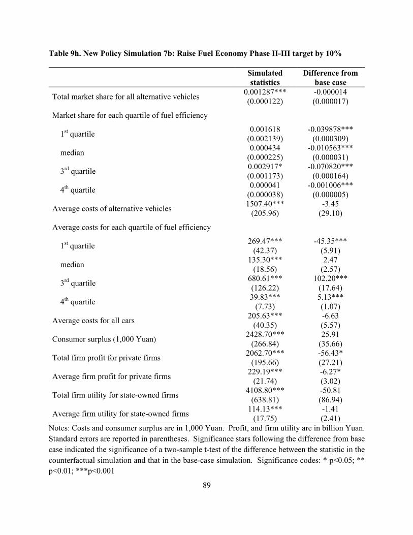
89

Table 9h. New Policy Simulation 7b: Raise Fuel Economy Phase II-III target by 10%

Simulated statistics

Difference from base case

Total market share for all alternative vehicles 0.001287*** (0.000122)

-0.000014 (0.000017)

Market share for each quartile of fuel efficiency � �

1st quartile 0.001618 (0.002139)

-0.039878*** (0.000309)

median 0.000434

(0.000225) -0.010563***

(0.000031)

3rd quartile 0.002917* (0.001173)

-0.070820*** (0.000164)

4th quartile 0.000041 (0.000038)

-0.001006*** (0.000005)

Average costs of alternative vehicles 1507.40*** (205.96)

-3.45 (29.10)

Average costs for each quartile of fuel efficiency �

1st quartile 269.47*** (42.37)

-45.35*** (5.91)

median 135.30***

(18.56) 2.47

(2.57)

3rd quartile 680.61*** (126.22)

102.20*** (17.64)

4th quartile 39.83***

(7.73) 5.13*** (1.07)

Average costs for all cars 205.63*** (40.35)

-6.63 (5.57)

Consumer surplus (1,000 Yuan) 2428.70*** (266.84)

25.91 (35.66)

Total firm profit for private firms 2062.70*** (195.66)

-56.43* (27.21)

Average firm profit for private firms 229.19*** (21.74)

-6.27* (3.02)

Total firm utility for state-owned firms 4108.80*** (638.81)

-50.81 (86.94)

Average firm utility for state-owned firms 114.13*** (17.75)

-1.41 (2.41)

Notes: Costs and consumer surplus are in 1,000 Yuan. Profit, and firm utility are in billion Yuan. Standard errors are reported in parentheses. Significance stars following the difference from base case indicated the significance of a two-sample t-test of the difference between the statistic in the counterfactual simulation and that in the base-case simulation. Significance codes: * p<0.05; ** p<0.01; ***p<0.001

90

Table 9i. New Policy Simulation 7c: Raise Fuel Economy Phase II-III target by 15%

Simulated statistics

Difference from base case

Total market share for all alternative vehicles 0.001260*** (0.000125)

-0.000041* (0.000017)

Market share for each quartile of fuel efficiency � �

1st quartile 0.001560 (0.002493)

-0.039936*** (0.000334)

median 0.000437

(0.000223) -0.010560***

(0.000031)

3rd quartile 0.002885** (0.001115)

-0.070852*** (0.000160)

4th quartile 0.000041 (0.000038)

-0.001006*** (0.000005)

Average costs of alternative vehicles 1500.60*** (204.70)

-10.28 (29.01)

Average costs for each quartile of fuel efficiency � �

1st quartile 269.47*** (45.96)

-45.35*** (6.17)

median 135.30***

(17.78) 2.47

(2.51)

3rd quartile 680.62*** (121.88)

102.21*** (17.33)

4th quartile 39.84***

(7.46) 5.14*** (1.05)

Average costs for all cars 203.56*** (38.85)

-8.70 (5.47)

Consumer surplus (1,000 Yuan) 2458.10*** (218.24)

55.31* (32.19)

Total firm profit for private firms 1971.80*** (204.00)

-147.29*** (27.81)

Average firm profit for private firms 219.09*** (22.67)

-16.37*** (3.09)

Total firm utility for state-owned firms 4096.80*** (568.15)

-62.79 (81.89)

Average firm utility for state-owned firms 113.80*** (15.78)

-1.74 (2.27)

Notes: Costs and consumer surplus are in 1,000 Yuan. Profit, and firm utility are in billion Yuan. Standard errors are reported in parentheses. Significance stars following the difference from base case indicated the significance of a two-sample t-test of the difference between the statistic in the counterfactual simulation and that in the base-case simulation. Significance codes: * p<0.05; ** p<0.01; ***p<0.001

91

Table 9j. New Policy Simulation 8a: Raise Corporate Average Fuel Consumption (CAFC) target by 5%

Simulated statistics

Difference from base case

Total market share for all alternative vehicles 0.001259*** (0.000127)

-0.000042* (0.000018)

Market share for each quartile of fuel efficiency

1st quartile 0.001601 (0.002220)

-0.039895*** (0.000314)

median 0.000420* (0.000213)

-0.010577*** (0.000030)

3rd quartile 0.002819* (0.001220)

-0.070918*** (0.000167)

4th quartile 0.000040 (0.000037)

-0.001007*** (0.000005)

Average costs of alternative vehicles 1500.40*** (203.89)

-10.47 (28.95)

Average costs for each quartile of fuel efficiency

1st quartile 269.47*** (41.16)

-45.35*** (5.83)

median 135.30***

(17.80) 2.47

(2.52)

3rd quartile 680.61*** (118.71)

102.20*** (17.11)

4th quartile 39.84***

(7.67) 5.13*** (1.06)

Average costs for all cars 195.05*** (38.03)

-17.21*** (5.41)

Consumer surplus (1,000 Yuan) 2510.30*** (254.11)

107.48*** (34.72)

Total firm profit for private firms 2014.90*** (192.83)

-104.22*** (27.00)

Average firm profit for private firms 223.88*** (21.43)

-11.58*** (3.00)

Total firm utility for state-owned firms 3998.60*** (558.67)

-161.02* (81.24)

Average firm utility for state-owned firms 111.07*** (15.52)

-4.47* (2.26)

Notes: Costs and consumer surplus are in 1,000 Yuan. Profit, and firm utility are in billion Yuan. Standard errors are reported in parentheses. Significance stars following the difference from base case indicated the significance of a two-sample t-test of the difference between the statistic in the counterfactual simulation and that in the base-case simulation. Significance codes: * p<0.05; ** p<0.01; ***p<0.001

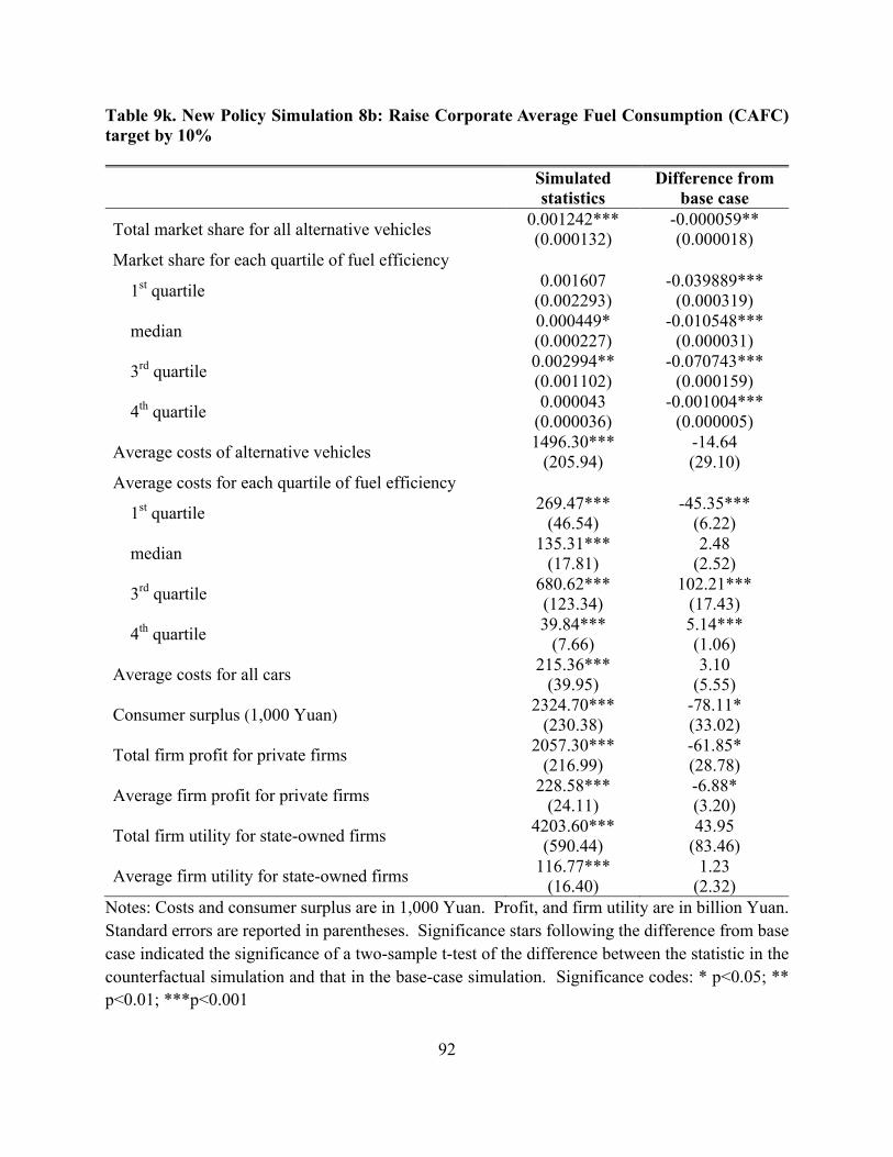
92

Table 9k. New Policy Simulation 8b: Raise Corporate Average Fuel Consumption (CAFC) target by 10%

Simulated statistics

Difference from base case

Total market share for all alternative vehicles 0.001242*** (0.000132)

-0.000059** (0.000018)

Market share for each quartile of fuel efficiency � �

1st quartile 0.001607 (0.002293)

-0.039889*** (0.000319)

median 0.000449* (0.000227)

-0.010548*** (0.000031)

3rd quartile 0.002994** (0.001102)

-0.070743*** (0.000159)

4th quartile 0.000043 (0.000036)

-0.001004*** (0.000005)

Average costs of alternative vehicles 1496.30*** (205.94)

-14.64 (29.10)

Average costs for each quartile of fuel efficiency

1st quartile 269.47*** (46.54)

-45.35*** (6.22)

median 135.31***

(17.81) 2.48

(2.52)

3rd quartile 680.62*** (123.34)

102.21*** (17.43)

4th quartile 39.84***

(7.66) 5.14*** (1.06)

Average costs for all cars 215.36*** (39.95)

3.10 (5.55)

Consumer surplus (1,000 Yuan) 2324.70*** (230.38)

-78.11* (33.02)

Total firm profit for private firms 2057.30*** (216.99)

-61.85* (28.78)

Average firm profit for private firms 228.58*** (24.11)

-6.88* (3.20)

Total firm utility for state-owned firms 4203.60*** (590.44)

43.95 (83.46)

Average firm utility for state-owned firms 116.77*** (16.40)

1.23 (2.32)

Notes: Costs and consumer surplus are in 1,000 Yuan. Profit, and firm utility are in billion Yuan. Standard errors are reported in parentheses. Significance stars following the difference from base case indicated the significance of a two-sample t-test of the difference between the statistic in the counterfactual simulation and that in the base-case simulation. Significance codes: * p<0.05; ** p<0.01; ***p<0.001

93

Table 9l. New Policy Simulation 8c: Raise Corporate Average Fuel Consumption (CAFC) target by 15%

Simulated statistics

Difference from base case

Total market share for all alternative vehicles 0.001349*** (0.000121)

0.000048** (0.000017)

Market share for each quartile of fuel efficiency � �

1st quartile 0.001786 (0.002349)

-0.039710*** (0.000323)

median 0.000470

(0.000225) -0.010527***

(0.000031)

3rd quartile 0.003106** (0.001160)

-0.070632*** (0.000163)

4th quartile 0.000043 (0.000035)

-0.001004*** (0.000005)

Average costs of alternative vehicles 1522.70*** (204.22)

11.75 (28.98)

Average costs for each quartile of fuel efficiency

1st quartile 269.48*** (42.76)

-45.34*** (5.94)

median 135.31***

(16.99) 2.48

(2.46)

3rd quartile 680.63*** (117.13)

102.22*** (17.00)

4th quartile 39.85***

(7.23) 5.15*** (1.03)

Average costs for all cars 235.32*** (36.62)

23.06*** (5.31)

Consumer surplus (1,000 Yuan) 2483.00*** (226.43)

80.16* (32.75)

Total firm profit for private firms 2205.50*** (188.77)

86.40*** (26.72)

Average firm profit for private firms 245.06*** (20.98)

9.60*** (2.97)

Total firm utility for state-owned firms 4424.90*** (544.68)

265.34*** (80.28)

Average firm utility for state-owned firms 122.91*** (15.13)

7.37*** (2.23)

Notes: Costs and consumer surplus are in 1,000 Yuan. Profit, and firm utility are in billion Yuan. Standard errors are reported in parentheses. Significance stars following the difference from base case indicated the significance of a two-sample t-test of the difference between the statistic in the counterfactual simulation and that in the base-case simulation. Significance codes: * p<0.05; ** p<0.01; ***p<0.001

94

Table 9m. New Policy Simulation 9a: Increase the target number of alternative vehicles for state-owned firms by 10

Simulated statistics

Difference from base case

Total market share for all alternative vehicles 0.001205*** (0.000123)

-0.000096*** (0.000017)

Market share for each quartile of fuel efficiency � �

1st quartile 0.001662 (0.002379)

-0.039834*** (0.000326)

median 0.000423

(0.000227) -0.010574***

(0.000031)

3rd quartile 0.002850* (0.001207)

-0.070887*** (0.000167)

4th quartile 0.000040 (0.000038)

-0.001007*** (0.000005)

Average costs of alternative vehicles 1487.10*** (204.82)

-23.82 (29.02)

Average costs for each quartile of fuel efficiency

1st quartile 269.46*** (44.36)

-45.36*** (6.06)

median 135.29***

(18.04) 2.46

(2.53)

3rd quartile 680.61*** (122.40)

102.20*** (17.36)

4th quartile 39.83***

(7.27) 5.13*** (1.03)

Average costs for all cars 195.65*** (38.71)

-16.61*** (5.46)

Consumer surplus (1,000 Yuan) 2601.10*** (263.38)

198.29*** (35.40)

Total firm profit for private firms 2032.90*** (195.10)

-86.25*** (27.17)

Average firm profit for private firms 225.87*** (21.68)

-9.59*** (3.02)

Total firm utility for state-owned firms 4016.00*** (602.85)

-143.59 (84.34)

Average firm utility for state-owned firms 111.56*** (16.75)

-3.98 (2.34)

Notes: Costs and consumer surplus are in 1,000 Yuan. Profit, and firm utility are in billion Yuan. Standard errors are reported in parentheses. Significance stars following the difference from base case indicated the significance of a two-sample t-test of the difference between the statistic in the counterfactual simulation and that in the base-case simulation. Significance codes: * p<0.05; ** p<0.01; ***p<0.001

95

Table 9n. New Policy Simulation 9b: Increase the target number of alternative vehicles for state-owned firms by 25

Simulated statistics

Difference from base case

Total market share for all alternative vehicles 0.001362*** (0.000116)

0.000061*** (0.000017)

Market share for each quartile of fuel efficiency � �

1st quartile 0.001810 (0.002350)

-0.039686*** (0.000323)

median 0.000466* (0.000237)

-0.010531*** (0.000032)

3rd quartile 0.003063** (0.001218)

-0.070674*** (0.000167)

4th quartile 0.000043 (0.000036)

-0.001004*** (0.000005)

Average costs of alternative vehicles 1525.90*** (205.04)

15.02 (29.04)

Average costs for each quartile of fuel efficiency �

1st quartile 269.46*** (43.97)

-45.36*** (6.03)

median 135.29***

(17.83) 2.46

(2.52)

3rd quartile 680.61*** (122.10)

102.20*** (17.34)

4th quartile 39.83***

(7.42) 5.13*** (1.04)

Average costs for all cars 229.00*** (38.46)

16.74*** (5.44)

Consumer surplus (1,000 Yuan) 2451.10*** (240.68)

48.29 (33.75)

Total firm profit for private firms 2220.00*** (195.42)

100.87*** (27.19)

Average firm profit for private firms 246.66*** (21.71)

11.20*** (3.02)

Total firm utility for state-owned firms 4352.10*** (585.10)

192.47* (83.08)

Average firm utility for state-owned firms 120.89*** (16.25)

5.35* (2.31)

Notes: Costs and consumer surplus are in 1,000 Yuan. Profit, and firm utility are in billion Yuan. Standard errors are reported in parentheses. Significance stars following the difference from base case indicated the significance of a two-sample t-test of the difference between the statistic in the counterfactual simulation and that in the base-case simulation. Significance codes: * p<0.05; ** p<0.01; ***p<0.001

96

Table 9o. New Policy Simulation 9c: Increase the target number of alternative vehicles for state-owned firms by 50

Simulated statistics

Difference from base case

Total market share for all alternative vehicles 0.001349*** (0.000119)

0.000048** (0.000017)

Market share for each quartile of fuel efficiency

1st quartile 0.001780 (0.002183)

-0.039716*** (0.000312)

median 0.000465* (0.000224)

-0.010532*** (0.000031)

3rd quartile 0.003096** (0.001129)

-0.070641*** (0.000161)

4th quartile 0.000043 (0.000036)

-0.001004*** (0.000005)

Average costs of alternative vehicles 1522.70*** (203.29)

11.79 (28.91)

Average costs for each quartile of fuel efficiency �

1st quartile 269.46*** (40.84)

-45.36*** (5.80)

median 135.29***

(17.33) 2.46

(2.48)

3rd quartile 680.61*** (118.23)

102.20*** (17.07)

4th quartile 39.83***

(7.33) 5.13*** (1.04)

Average costs for all cars 233.98*** (36.87)

21.72*** (5.33)

Consumer surplus (1,000 Yuan) 2483.10*** (232.65)

80.26* (33.18)

Total firm profit for private firms 2222.00*** (185.36)

102.90*** (26.48)

Average firm profit for private firms 246.89*** (20.60)

11.43*** (2.94)

Total firm utility for state-owned firms 4417.20*** (549.89)

257.58*** (80.64)

Average firm utility for state-owned firms 122.70*** (15.28)

7.16*** (2.24)

Notes: Costs and consumer surplus are in 1,000 Yuan. Profit, and firm utility are in billion Yuan. Standard errors are reported in parentheses. Significance stars following the difference from base case indicated the significance of a two-sample t-test of the difference between the statistic in the counterfactual simulation and that in the base-case simulation. Significance codes: * p<0.05; ** p<0.01; ***p<0.001

97

Appendix A

98

Figure A1: Market Structure of Chinese Automobile Industry

Notes: Chinese firms that are at least partially state-owned are in green. Private Chinese firms are in yellow. Interactional car companies are in blue. Lines connecting firms indicate joint ventures between firms. Source: Hu, Xiao and Zhou (2014)

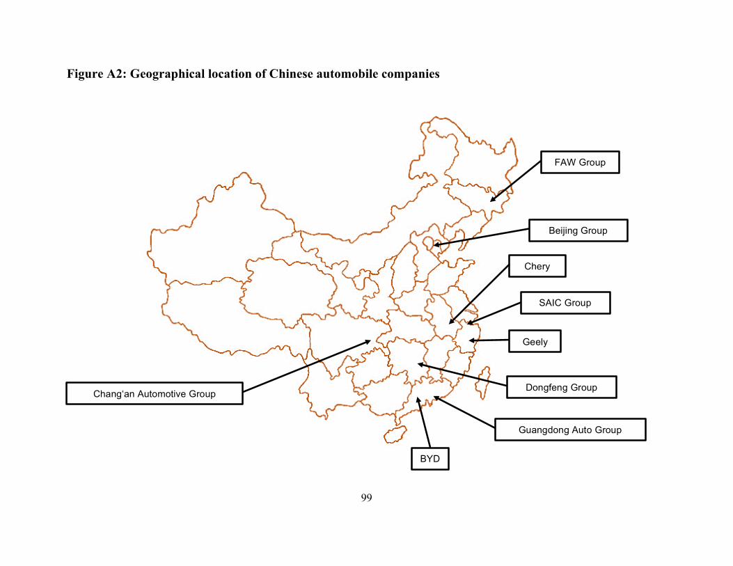
99

Figure A2: Geographical location of Chinese automobile companies

FAW Group

SAIC Group

Dongfeng Group

Guangdong Auto Group

Beijing Group

Chang‘an Automotive Group

Chery

Geely

BYD

100

Table A1. First-stage F-statistics: Different objectives for state-owned model with “has international joint venture dummy” interactions

Endogenous variables Instruments Chosen First-Stage F-Statistic

Alternative Fuel Vehicle Number of cars with similar values of:

- Fuel efficiency - Length - Weight - Capacity - Horsepower

Value for the closest car of:

- Fuel efficiency - Length - Weight - Horsepower

Value for the closest car with a different model-year-displacement of:

- Fuel efficiency - Weight

Fraction of other cars that year that are alternative vehicles Has international joint venture dummy interacted with:

- Fraction of other cars that year that are alternative vehicles - Number of cars with similar values of fuel efficiency - Number of cars with similar values of horsepower

8.810

Fuel Efficiency 49.500

Length 112.340

Weight 95.140

Capacity 1224.520

Horsepower 131.090

Price 99.350

Quantity 10.770

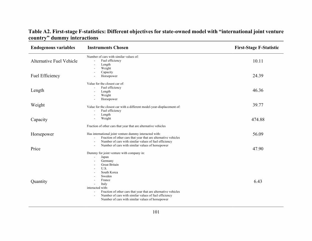
101

Table A2. First-stage F-statistics: Different objectives for state-owned model with “international joint venture country” dummy interactions

Endogenous variables Instruments Chosen First-Stage F-Statistic

Alternative Fuel Vehicle Number of cars with similar values of:

- Fuel efficiency - Length - Weight - Capacity - Horsepower

Value for the closest car of:

- Fuel efficiency - Length - Weight - Horsepower

Value for the closest car with a different model-year-displacement of:

- Fuel efficiency - Length - Weight

Fraction of other cars that year that are alternative vehicles Has international joint venture dummy interacted with:

- Fraction of other cars that year that are alternative vehicles - Number of cars with similar values of fuel efficiency - Number of cars with similar values of horsepower

Dummy for joint venture with company in:

- Japan - Germany - Great Britain - U.S. - South Korea - Sweden - France - Italy

interacted with: - Fraction of other cars that year that are alternative vehicles - Number of cars with similar values of fuel efficiency

Number of cars with similar values of horsepower

10.11

Fuel Efficiency 24.39

Length 46.36

Weight 39.77

Capacity 474.88

Horsepower 56.09

Price 47.90

Quantity 6.43

102

Appendix B

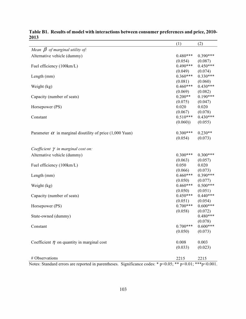
103

Table B1. Results of model with interactions between consumer preferences and price, 2010-2013 (1) (2) Mean β of marginal utility of: Alternative vehicle (dummy) 0.480***

(0.054) 0.390*** (0.087)

Fuel efficiency (100km/L) 0.490*** (0.049)

0.450*** (0.074)

Length (mm) 0.360*** (0.081)

0.330*** (0.060)

Weight (kg) 0.460*** (0.069)

0.430*** (0.082)

Capacity (number of seats) 0.200** (0.075)

0.190*** (0.047)

Horsepower (PS) 0.020 (0.067)

0.020 (0.078)

Constant 0.510*** (0.060))

0.430*** (0.055)

Parameter α in marginal disutility of price (1,000 Yuan) 0.300***

(0.054) 0.230** (0.073)

Coefficient γ in marginal cost on: Alternative vehicle (dummy) 0.300***

(0.063) 0.300*** (0.057)

Fuel efficiency (100km/L) 0.050 (0.066)

0.020 (0.073)

Length (mm) 0.460*** (0.050)

0.390*** (0.077)

Weight (kg) 0.460*** (0.050)

0.500*** (0.051)

Capacity (number of seats) 0.450*** (0.051)

0.440*** (0.054)

Horsepower (PS) 0.700*** (0.058)

0.600*** (0.072)

State-owned (dummy) 0.480*** (0.078)

Constant 0.700*** (0.050)

0.600*** (0.073)

Coefficient η on quantity in marginal cost 0.008

(0.033) 0.003 (0.023)

# Observations 2215 2215

Notes: Standard errors are reported in parentheses. Significance codes: * p<0.05; ** p<0.01; ***p<0.001.

104

Table B2. Results of model with full set of interactions between consumer preferences and product characteristics, 2010-2013

(1)

(2) Mean β of marginal utility of: Alternative vehicle (dummy) 0.190***

(0.025) 0.700*** (0.004)

Fuel efficiency (100km/L) 0.050* (0.021)

0.600*** (0.012)

Length (m) 0.160*** (0.033)

0.150*** (0.007)

Weight (metric ton) 0.170*** (0.032)

0.380*** (0.006)

Capacity (number of seats) 0.040 (0.029)

-0.130*** (0.004)

Horsepower (PS) 0.210*** (0.023)

0.370*** (0.003)

Constant 0.080* (0.032)

0.150*** (0.001)

Standard deviation σ of marginal utility of: Alternative vehicle (dummy) 0.160***

(0.042) 0.200*** (0.004)

Fuel efficiency (100km/L) 0.450*** (0.055)

0.420 *** (0.005)

Length (m) 0.510*** (0.054)

0.020*** (0.004)

Weight (metric ton) 0.230*** (0.028)

0.250*** (0.005)

Capacity (number of seats) 0.030 (0.021)

0.480*** (0.010)

Horsepower (0.01PS) 0.350*** (0.044)

0.330*** (0.007)

Constant 0.080*** (0.027)

0.400*** (0.005)

Parameter α in marginal disutility of price (10,000 yuan) 0.480***

(0.057) 0.330*** (0.005)

Coefficient γ in marginal cost on: Alternative vehicle (dummy) 0.230***

(0.027) 0.450*** (0.003)

Fuel efficiency (100km/L) 0.290*** (0.046)

0.280*** (0.002)

Length (m) 0.070*** (0.019)

0.190*** (0.006)

Weight (metric ton) 0.170*** 0.020***

105

(0.034) (0.004) Capacity (number of seats) 0.360***

(0.041) 0.700*** (0.004)

Horsepower (0.01PS) 0.600*** (0.061)

0.150*** (0.006)

State-owned (dummy) 0.110*** (0.012)

Constant 0.160*** (0.026)

0.130*** (0.006)

Coefficient η on quantity in marginal cost 0.010***

(0.002) 0.001** (0.000)

# Observations 2215 2215

Notes: Standard errors are reported in parentheses. Significance codes: * p<0.05; ** p<0.01; ***p<0.001.

106

Table B3. Model with international joint venture dummies, possibly allowing stated-owned firms to have different objectives, 2010-2013 (1) (2) Mean β of marginal utility of: Alternative vehicle (dummy) 0.054***

(0.000) 0.075*** (0.010)

Fuel efficiency (100km/L) 0.067*** (0.000)

0.137** (0.047)

Length (m) 0.181*** (0.000)

0.154*** (0.011)

Weight (metric ton) 0.015*** (0.000)

0.059*** (0.018)

Capacity (number of seats) 0.415*** (0.000)

0.131*** (0.018)

Horsepower (PS) 1.200*** (0.000)

0.022 (0.012)

Constant 0.133 (0.000)

0.056* (0.025)

Standard deviation σ of marginal utility of:

Alternative vehicle (dummy) 0.120*** (0.000)

0.033** (0.014)

Fuel efficiency (100km/L) 0.651*** (0.000)

0.154*** (0.017)

Length (m) 0.283*** (0.000)

0.132*** (0.010)

Weight (metric ton) 0.473*** (0.000)

0.008 (0.010)

Capacity (number of seats) 0.078*** (0.000)

0.038*** (0.009)

Horsepower (0.01PS) 0.014*** (0.000)

0.170*** (0.008)

Constant 0.001*** (0.000)

0.021 (0.015)

Parameter α in marginal disutility of price (1,000 Yuan) 0.258***

(0.000) 0.271*** (0.013)

Coefficient γ in marginal cost on: Alternative vehicle (dummy) 0.738***

(0.000) 0.056* (0.022)

Fuel efficiency (100km/L) 0.466*** (0.000)

0.071** (0.022)

Length (m) 0.778*** (0.000)

0.125*** (0.009)

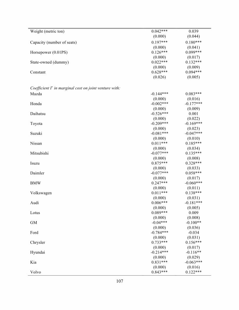
107

Weight (metric ton) 0.042*** (0.000)

0.039 (0.044)

Capacity (number of seats) 0.197*** (0.000)

0.180*** (0.041)

Horsepower (0.01PS) 0.126*** (0.000)

0.099*** (0.017)

State-owned (dummy) 0.022*** (0.000)

0.132*** (0.009)

Constant 0.628*** (0.026)

0.094*** (0.005)

Coefficient ! in marginal cost on joint venture with: Mazda -0.144***

(0.000) 0.083*** (0.016)

Honda -0.002*** (0.000)

-0.177*** (0.009)

Daihatsu -0.526*** (0.000)

0.001 (0.022)

Toyota -0.209*** (0.000)

-0.169*** (0.023)

Suzuki -0.081*** (0.000)

-0.047*** (0.010)

Nissan 0.011*** (0.000)

0.185*** (0.034)

Mitsubishi -0.077*** (0.000)

0.135*** (0.008)

Isuzu 0.875*** (0.000)

0.328*** (0.033)

Daimler -0.077*** (0.000)

0.058*** (0.017)

BMW 0.247*** (0.000)

-0.060*** (0.011)

Volkswagen 0.011*** (0.000)

0.138*** (0.031)

Audi 0.006*** (0.000)

-0.181*** (0.005)

Lotus 0.089*** (0.000)

0.009 (0.008)

GM -0.04*** (0.000)

-0.100** (0.036)

Ford -0.784*** (0.000)

-0.034 (0.031)

Chrysler 0.733*** (0.000)

0.156*** (0.017)

Hyundai -0.214*** (0.000)

-0.116** (0.029)

Kia 0.831*** (0.000)

-0.063*** (0.016)

Volvo 0.843*** 0.122***

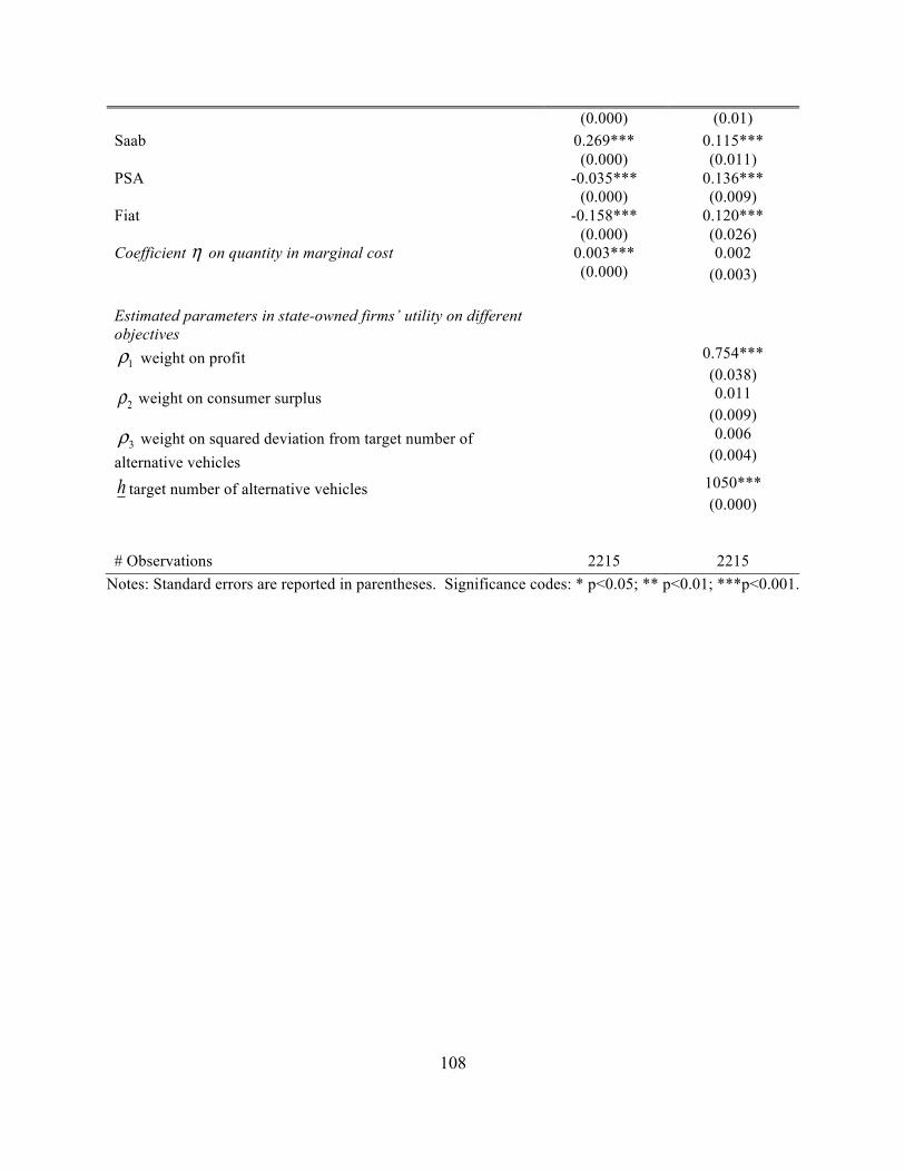
108

(0.000) (0.01) Saab 0.269***

(0.000) 0.115*** (0.011)

PSA -0.035*** (0.000)

0.136*** (0.009)

Fiat -0.158*** (0.000)

0.120*** (0.026)

Coefficient η on quantity in marginal cost 0.003*** (0.000)

0.002 (0.003)

Estimated parameters in state-owned firms’ utility on different objectives

1ρ weight on profit 0.754*** (0.038)

2ρ weight on consumer surplus 0.011 (0.009)

3ρ weight on squared deviation from target number of alternative vehicles

0.006 (0.004)

h target number of alternative vehicles 1050*** (0.000)

# Observations 2215 2215 Notes: Standard errors are reported in parentheses. Significance codes: * p<0.05; ** p<0.01; ***p<0.001.

109

Table B4. Model include interaction with “has international joint venture” dummy, possibly allowing stated-owned firms to have different objectives, 2010-2013 (1) (2) Mean " of marginal utility of: Alternative vehicle (dummy) 0.054***

(0.000) 0.210*** (0.003)

Fuel efficiency (100km/L) 0.067*** (0.000)

0.211*** (0.002)

Length (m) 0.181*** (0.000)

0.017*** (0.002)

Weight (metric ton) 0.015*** (0.000)

0.220*** (0.001)

Capacity (number of seats) 0.415*** (0.000)

0.005*** (0.001)

Horsepower (PS) 1.200*** (0.000)

0.079*** (0.004)

Constant 0.133*** (0.000)

0.118*** (0.006)

Standard deviation # of marginal utility of: Alternative vehicle (dummy) 0.120***

(0.000) 0.107*** (0.005)

Fuel efficiency (100km/L) 0.651*** (0.000)

0.133*** (0.005)

Length (m) 0.283*** (0.000)

0.078*** (0.002)

Weight (metric ton) 0.473*** (0.000)

0.187*** (0.001)

Capacity (number of seats) 0.078*** (0.000)

0.065*** (0.005)

Horsepower (0.01PS) 0.014*** (0.000)

0.046*** (0.007)

Constant 0.001*** (0.000)

0.207*** (0.005)

Parameter $ in marginal disutility of price (1,000 Yuan)

0.258*** (0.000)

0.348*** (0.001)

Coefficient % in marginal cost on: Alternative vehicle (dummy) 0.738***

(0.000) 0.241*** (0.006)

Fuel efficiency (100km/L) 0.466*** (0.000)

0.093*** (0.000)

Length (m) 0.778*** (0.000)

0.113*** (0.003)

Weight (metric ton) 0.042*** 0.121***

110

(0.000) (0.003) Capacity (number of seats) 0.197***

(0.000) 0.230*** (0.005)

Horsepower (0.01PS) 0.126*** (0.000)

0.157*** (0.009)

State-owned (dummy) 0.022*** (0.000)

0.177*** (0.003)

Constant 0.628*** (0.000)

0.191*** (0.003)

Coefficient ! in marginal cost on joint venture with: Mazda -0.144***

(0.000) 0.105*** (0.003)

Honda -0.002*** (0.000)

0.085*** (0.003)

Daihatsu -0.526*** (0.000)

-0.181*** (0.008)

Toyota -0.209*** (0.000)

-0.134*** (0.009)

Suzuki -0.081*** (0.000)

0.012*** (0.003)

Nissan 0.011*** (0.000)

-0.029*** (0.005)

Mitsubishi -0.077*** (0.000)

-0.012*** (0.002)

Isuzu 0.875*** (0.000)

-0.092*** (0.002)

Daimler -0.077*** (0.000)

-0.237*** (0.003)

BMW 0.247*** (0.000)

-0.081*** (0.003)

Volkswagen 0.011*** (0.000)

-0.033*** (0.004)

Audi 0.006*** (0.000)

-0.151*** (0.001)

Lotus 0.089*** (0.000)

-0.245*** (0.006)

GM -0.040*** (0.000)

-0.225*** (0.002)

Ford -0.784*** (0.000)

-0.051*** (0.007)

Chrysler 0.733*** (0.000)

-0.037*** (0.001)

Hyundai -0.214*** (0.000)

0.024** (0.009)

Kia 0.831*** (0.000)

0.159*** (0.006)

Volvo 0.843*** (0.000)

0.025* (0.010)

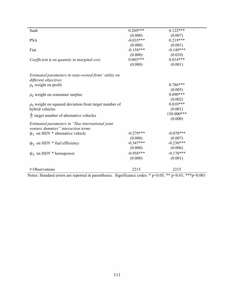
111

Saab 0.269*** (0.000)

0.122*** (0.007)

PSA -0.035*** (0.000)

0.219*** (0.001)

Fiat -0.158*** (0.000)

-0.149*** (0.010)

Coefficient & on quantity in marginal cost 0.003*** (0.000)

0.014*** (0.001)

Estimated parameters in state-owned firms’ utility on different objectives

'(weight on profit 0.786*** (0.005)

'*weight on consumer surplus 0.090*** (0.002)

'+weight on squared deviation from target number of hybrid vehicles

0.010*** (0.001)

h target number of alternative vehicles 150.000*** (0.000)

Estimated parameters in “Has international joint venture dummies” interaction terms

,(on HIJV * alternative vehicle -0.279*** (0.000)

-0.070*** (0.007)

,*on HIJV * fuel efficiency -0.547*** (0.000)

-0.230*** (0.006)

,+on HIJV * horsepower -0.958*** (0.000)

-0.170*** (0.001)

# Observations 2215 2215

Notes: Standard errors are reported in parentheses. Significance codes: * p<0.05; ** p<0.01; ***p<0.001

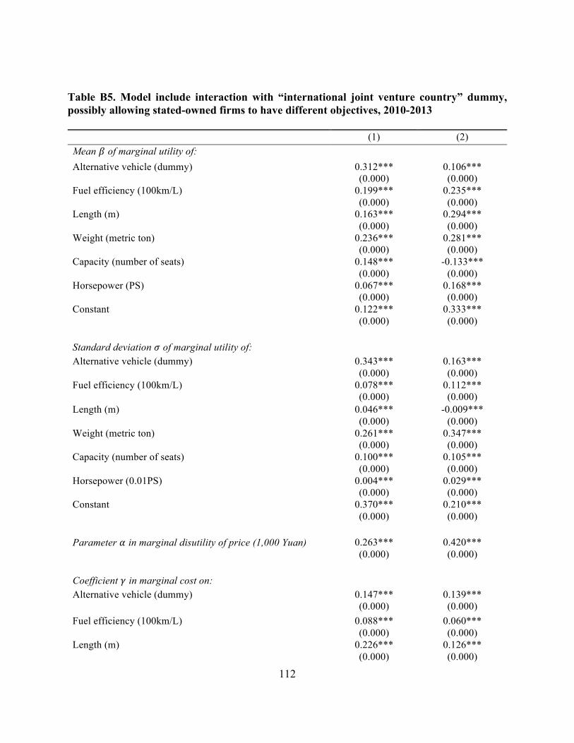
112

Table B5. Model include interaction with “international joint venture country” dummy, possibly allowing stated-owned firms to have different objectives, 2010-2013 (1) (2) Mean " of marginal utility of: Alternative vehicle (dummy) 0.312***

(0.000) 0.106*** (0.000)

Fuel efficiency (100km/L) 0.199*** (0.000)

0.235*** (0.000)

Length (m) 0.163*** (0.000)

0.294*** (0.000)

Weight (metric ton) 0.236*** (0.000)

0.281*** (0.000)

Capacity (number of seats) 0.148*** (0.000)

-0.133*** (0.000)

Horsepower (PS) 0.067*** (0.000)

0.168*** (0.000)

Constant 0.122*** (0.000)

0.333*** (0.000)

Standard deviation # of marginal utility of: Alternative vehicle (dummy) 0.343***

(0.000) 0.163*** (0.000)

Fuel efficiency (100km/L) 0.078*** (0.000)

0.112*** (0.000)

Length (m) 0.046*** (0.000)

-0.009*** (0.000)

Weight (metric ton) 0.261*** (0.000)

0.347*** (0.000)

Capacity (number of seats) 0.100*** (0.000)

0.105*** (0.000)

Horsepower (0.01PS) 0.004*** (0.000)

0.029*** (0.000)

Constant 0.370*** (0.000)

0.210*** (0.000)

Parameter $ in marginal disutility of price (1,000 Yuan) 0.263***

(0.000) 0.420*** (0.000)

Coefficient % in marginal cost on: Alternative vehicle (dummy) 0.147***

(0.000) 0.139*** (0.000)

Fuel efficiency (100km/L) 0.088*** (0.000)

0.060*** (0.000)

Length (m) 0.226*** (0.000)

0.126*** (0.000)

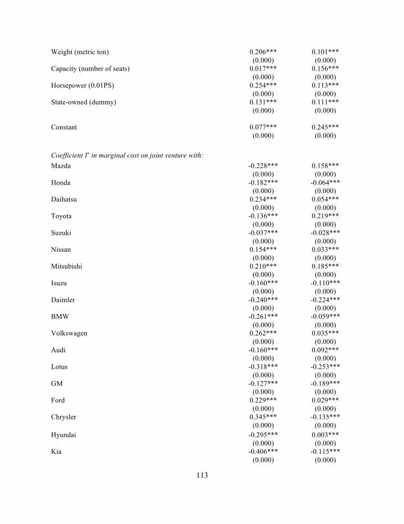
113

Weight (metric ton) 0.206*** (0.000)

0.101*** (0.000)

Capacity (number of seats) 0.017*** (0.000)

0.156*** (0.000)

Horsepower (0.01PS) 0.254*** (0.000)

0.113*** (0.000)

State-owned (dummy) 0.131*** (0.000)

0.111*** (0.000)

Constant 0.077*** (0.000)

0.245*** (0.000)

Coefficient ! in marginal cost on joint venture with: Mazda -0.228***

(0.000) 0.158*** (0.000)

Honda -0.182*** (0.000)

-0.064*** (0.000)

Daihatsu 0.234*** (0.000)

0.054*** (0.000)

Toyota -0.136*** (0.000)

0.219*** (0.000)

Suzuki -0.037*** (0.000)

-0.028*** (0.000)

Nissan 0.154*** (0.000)

0.033*** (0.000)

Mitsubishi 0.210*** (0.000)

0.185*** (0.000)

Isuzu -0.160*** (0.000)

-0.110*** (0.000)

Daimler -0.240*** (0.000)

-0.224*** (0.000)

BMW -0.261*** (0.000)

-0.059*** (0.000)

Volkswagen 0.262*** (0.000)

0.035*** (0.000)

Audi -0.160*** (0.000)

0.092*** (0.000)

Lotus -0.318*** (0.000)

-0.253*** (0.000)

GM -0.127*** (0.000)

-0.189*** (0.000)

Ford 0.229*** (0.000)

0.029*** (0.000)

Chrysler 0.345*** (0.000)

-0.135*** (0.000)

Hyundai -0.295*** (0.000)

0.003*** (0.000)

Kia -0.406*** (0.000)

-0.115*** (0.000)

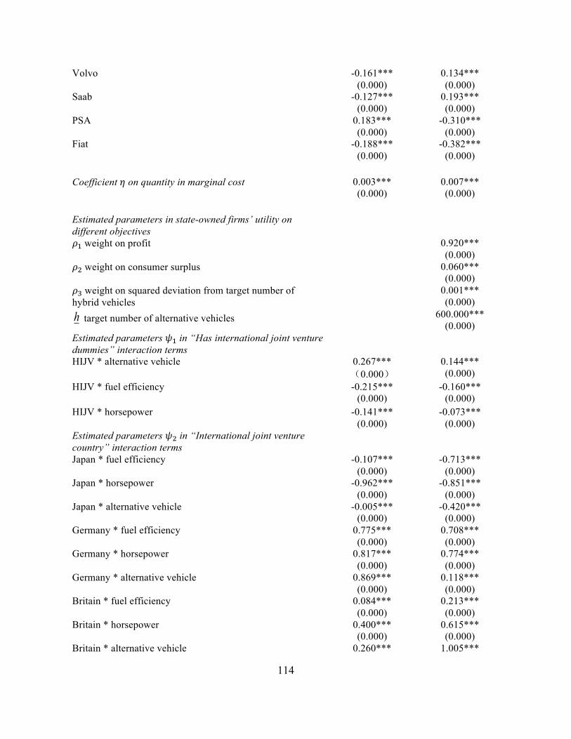
114

Volvo -0.161*** (0.000)

0.134*** (0.000)

Saab -0.127*** (0.000)

0.193*** (0.000)

PSA 0.183*** (0.000)

-0.310*** (0.000)

Fiat -0.188*** (0.000)

-0.382*** (0.000)

Coefficient & on quantity in marginal cost 0.003***

(0.000) 0.007*** (0.000)

Estimated parameters in state-owned firms’ utility on different objectives

'(weight on profit 0.920*** (0.000)

'*weight on consumer surplus 0.060*** (0.000)

'+weight on squared deviation from target number of hybrid vehicles

0.001*** (0.000)

h target number of alternative vehicles 600.000*** (0.000)

Estimated parameters ,(in “Has international joint venture dummies” interaction terms

HIJV * alternative vehicle 0.267*** �0.000�

0.144*** (0.000)

HIJV * fuel efficiency -0.215*** (0.000)

-0.160*** (0.000)

HIJV * horsepower -0.141*** (0.000)

-0.073*** (0.000)

Estimated parameters ,*in “International joint venture country” interaction terms

Japan * fuel efficiency -0.107*** (0.000)

-0.713*** (0.000)

Japan * horsepower -0.962*** (0.000)

-0.851*** (0.000)

Japan * alternative vehicle -0.005*** (0.000)

-0.420*** (0.000)

Germany * fuel efficiency 0.775*** (0.000)

0.708*** (0.000)

Germany * horsepower 0.817*** (0.000)

0.774*** (0.000)

Germany * alternative vehicle 0.869*** (0.000)

0.118*** (0.000)

Britain * fuel efficiency 0.084*** (0.000)

0.213*** (0.000)

Britain * horsepower 0.400*** (0.000)

0.615*** (0.000)

Britain * alternative vehicle 0.260*** 1.005***

115

(0.000) (0.000) US * fuel efficiency -0.800***

(0.000) -0.149***

(0.000) US * horsepower -0.431***

(0.000) -0.662***

(0.000) US * alternative vehicle -0.911***

(0.000) -0.203***

(0.000) South Korea * fuel efficiency 0.182***

(0.000) 0.678*** (0.000)

South Korea * horsepower 0.264*** (0.000)

0.361*** (0.000)

South Korea * alternative vehicle 0.146*** (0.000)

0.445*** (0.000)

Sweden * fuel efficiency 0.136*** (0.000)

0.748*** (0.000)

Sweden * horsepower 0.869*** (0.000)

0.912*** (0.000)

Sweden * alternative vehicle 0.580*** (0.000)

0.981*** (0.000)

France * fuel efficiency 0.550*** (0.000)

0.437*** (0.000)

France * horsepower 0.145*** (0.000)

0.203*** (0.000)

France * alternative vehicle 0.853*** (0.000)

0.268*** (0.000)

Italy * fuel efficiency 0.622*** (0.000)

0.336*** (0.000)

Italy * horsepower 0.351*** (0.000)

1.042*** (0.000)

Italy * alternative vehicle 0.513*** (0.000)

0.098*** (0.000)

# Observations 2215 2215 Notes: Standard errors are reported in parentheses. Significance codes: * p<0.05; ** p<0.01; ***p<0.001

116

Table B6. Welfare for the model without “has international joint venture” interactions, possibly allowing stated-owned firms to have different objectives, 2010-2013 2010 2011 2012 2013

Consumer surplus 1,717.00 941.41 303.96 459.07 (2,549.20) (1,508.20) (839.45) (915.82) Total firm profit for private firms 865.99*** 615.70*** 788.84*** 1,949.60*** (2.15) (1.37) (1.19) (3.40) Average firm profit for private firms 86.60*** 61.57*** 87.650*** 216.63*** (2.15) (0.14) (0.13) (0.38) Total firm utility for state-owned firms 1,662.70*** 2,405.60*** 2,506.70*** 3,432.10*** (182.19) (173.00) (146.73) (197.78) Average firm utility for state-owned firms 63.95*** 82.95*** 80.86*** 95.34*** (700.71) (5.97) (4.73) (5.49)

Notes: All values are in units of billion Yuan. Standard errors are reported in parentheses. Significance codes: * p<0.05; ** p<0.01; ***p<0.001

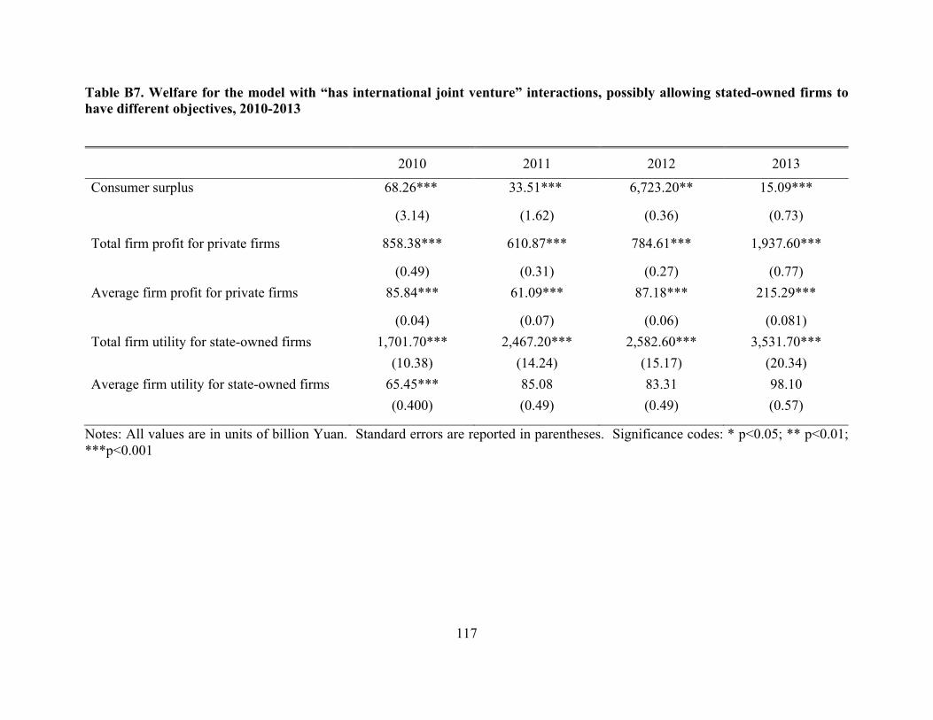
117

Table B7. Welfare for the model with “has international joint venture” interactions, possibly allowing stated-owned firms to have different objectives, 2010-2013

2010 2011 2012 2013

Consumer surplus 68.26*** 33.51*** 6,723.20** 15.09***

(3.14) (1.62) (0.36) (0.73)

Total firm profit for private firms 858.38*** 610.87*** 784.61*** 1,937.60***

(0.49) (0.31) (0.27) (0.77) Average firm profit for private firms 85.84*** 61.09*** 87.18*** 215.29***

(0.04) (0.07) (0.06) (0.081) Total firm utility for state-owned firms 1,701.70*** 2,467.20*** 2,582.60*** 3,531.70*** (10.38) (14.24) (15.17) (20.34) Average firm utility for state-owned firms 65.45*** 85.08 83.31 98.10 (0.400) (0.49) (0.49) (0.57)

Notes: All values are in units of billion Yuan. Standard errors are reported in parentheses. Significance codes: * p<0.05; ** p<0.01; ***p<0.001

118

Table B8. Welfare for the model with international joint venture country interactions, allowing stated-owned firms to have different objectives, 2010-2013

2010 2011 2012 2013 Consumer surplus 13.43*** 6.70*** 0.80*** 2.64*** (0.51) (0.23) (0.03) (0.10) Total firm profit for private firms 858.38*** 610.87*** 784.61*** 1,937.60*** (0.00) (0.00) (0.00) (0.00) Average firm profit for private firms 85.84*** 61.09*** 87.18*** 215.29*** (0.22) (0.14) (0.13) (0.38) Total firm utility for state-owned firms 1,985.50*** 2,884.90*** 3,022.40* 4,132.50*** (0.03) (0.14) (0.00) (0.01) Average firm utility for state-owned firms 76.37*** 99.48*** 97.50*** 114.79*** (0.00) (0.00) (0.00) (0.00)

Notes: All values are in units of billion Yuan. Standard errors are reported in parentheses. Significance codes: * p<0.05; ** p<0.01; ***p<0.001

119

Table B9. Welfare for the model with fuel economy standard interactions, allowing stated-owned firms to have different objectives, 2010-2013 2010 2011 2012 2013 Consumer surplus 70.85*** 34.84*** 7.01*** 15.89*** (5.56) (3.17) (0.73) (1.31) Total firm profit for private firms 858.38*** 610.87*** 784.61*** 1,937.60*** (0.69) (0.44) (0.38) (1.09) Average firm profit for private firms 85.84*** 61.09*** 87.180*** 215.29*** (0.07) (0.04) (0.42) (0.12) Total firm utility for state-owned firms 1,701.90*** 2,467.40*** 2,582.60*** 3,531.80*** (3.93) (5.72) (4.980) (7.51) Average firm utility for state-owned firms 65.46*** 85.08*** 83.31*** 98.105*** (0.15) (0.20) (0.16) (0.21)

Notes: All values are in units of billion Yuan. Standard errors are reported in parentheses. Significance codes: * p<0.05; ** p<0.01; ***p<0.001

120

Table B10. Welfare for the the State-owned fuel economy model with “international joint venture country” dummy interactions including interactions between dummies for international joint ventures with each US and Japan car company interacted with the technology-related car characteristics 2010 2011 2012 2013 Consumer surplus 13.92*** 7.20*** 0.82*** 2.63*** (1183.20) (588.24) (79.44) (234.57) Total firm profit for private firms 862.82*** 613.69*** 787.08*** 1944.60*** (0.60) (0.38) (0.33) (0.94) Average firm profit for private firms 86.28*** 61.37*** 87.45*** 216.07*** (0.06) (0.04) (0.04) (0.10) Total firm utility for state-owned firms 2165.50*** 3154.30*** 3300.40*** 4517.90*** (1.15) (2.59) (2.10) (3.55) Average firm utility for state-owned firms 83.29*** 108.77*** 106.47*** 125.50*** (0.04) (0.09) (0.07) (0.10)

Notes: All values are in units of billion Yuan. Standard errors are reported in parentheses. Significance codes: * p<0.05; ** p<0.01; ***p<0.001

121

Appendix C

122

Table C1. Model with international joint venture dummies allowing stated-owned firms to have different objectives, 2010-2013 (2) (3) Mean β of marginal utility of: Alternative vehicle (dummy) 0.075***

(0.010) 0.163*** (0.000)

Fuel efficiency (100km/L) 0.137** (0.047)

0.195*** (0.000)

Length (m) 0.154*** (0.011)

0.229*** (0.000)

Weight (metric ton) 0.059*** (0.018)

0.163*** (0.000)

Capacity (number of seats) 0.131*** (0.018)

0.221*** (0.000)

Horsepower (PS) 0.022 (0.012)

0.145*** (0.000)

Constant 0.056* (0.025)

0.154*** (0.000)

Standard deviation σ of marginal utility of:

Alternative vehicle (dummy) 0.033** (0.014)

Fuel efficiency (100km/L) 0.154*** (0.017)

Length (m) 0.132*** (0.010)

Weight (metric ton) 0.008 (0.010)

Capacity (number of seats) 0.038*** (0.009)

Horsepower (0.01PS) 0.170*** (0.008)

Constant 0.021 (0.015)

Parameter α in marginal disutility of price (1,000 Yuan) 0.271***

(0.013) 0.087*** (0.001)

Coefficient γ in marginal cost on: Alternative vehicle (dummy) 0.056*

(0.022) 0.153*** (0.000)

Fuel efficiency (100km/L) 0.071** (0.022)

0.161*** (0.000)

Length (m) 0.125*** (0.009)

0.188*** (0.000)

123

Weight (metric ton) 0.039 (0.044)

0.146*** (0.000)

Capacity (number of seats) 0.180*** (0.041)

0.214*** (0.000)

Horsepower (0.01PS) 0.099*** (0.017)

0.177*** (0.000)

State-owned (dummy) 0.132*** (0.009)

0.191*** (0.000)

Constant 0.094*** (0.005)

0.172*** (0.000)

Coefficient ! in marginal cost on joint venture with: Mazda 0.083***

(0.016) 0.311*** (0.000)

Honda -0.177*** (0.009)

-0.923*** (0.000)

Daihatsu 0.001 (0.022)

0.430*** (0.000)

Toyota -0.169*** (0.023)

0.185*** (0.000)

Suzuki -0.047*** (0.010)

-0.905*** (0.000)

Nissan 0.185*** (0.034)

-0.980*** (0.000)

Mitsubishi 0.135*** (0.008)

-0.439*** (0.000)

Isuzu 0.328*** (0.033)

0.111*** (0.000)

Daimler 0.058*** (0.017)

-0.258*** (0.000)

BMW -0.060*** (0.011)

0.409*** (0.000)

Volkswagen 0.138*** (0.031)

0.595*** (0.000)

Audi -0.181*** (0.005)

0.262*** (0.000)

Lotus 0.009 (0.008)

0.603*** (0.000)

GM -0.100** (0.036)

-0.711*** (0.000)

Ford -0.034 (0.031)

0.222*** (0.000)

Chrysler 0.156*** (0.017)

-0.117*** (0.000)

Hyundai -0.116** (0.029)

0.297*** (0.000)

Kia -0.063*** (0.016)

-0.319*** (0.000)

Volvo 0.122*** 0.424***

124

(0.01) (0.000) Saab 0.115***

(0.011) -0.508***

(0.000) PSA 0.136***

(0.009) -0.086***

(0.000) Fiat 0.120***

(0.026) -0.262***

(0.000) Coefficient η on quantity in marginal cost 0.002

(0.003) 0.002*** (0.000)

Estimated parameters in state-owned firms’ utility on different objectives

1ρ weight on profit 0.754*** (0.038)

0.312*** (0.021)

2ρ weight on consumer surplus 0.011 (0.009)

0.301*** (0.000)

3ρ weight on squared deviation from target number of alternative vehicles

0.006 (0.004)

0.091*** (0.000)

h target number of alternative vehicles 1050*** (0.000)

650.000*** (0.000)

# Observations 2215 2215

Notes: Standard errors are reported in parentheses. Significance codes: * p<0.05; ** p<0.01; ***p<0.001. Specification (2) is the random coefficient model and specification (3) is the traditional logit model without any interaction between consumer characteristics and product characteristics.

125

Table C2. Model with international joint venture dummies allowing stated-owned firms to have different objectives, 2010-2013 (2) (3) Mean β of marginal utility of: Alternative vehicle (dummy) 0.075***

(0.010) 0.163*** (0.000)

Fuel efficiency (100km/L) 0.137** (0.047)

0.195*** (0.000)

Length (m) 0.154*** (0.011)

0.229*** (0.000)

Weight (metric ton) 0.059*** (0.018)

0.163*** (0.000)

Capacity (number of seats) 0.131*** (0.018)

0.221*** (0.000)

Horsepower (PS) 0.022 (0.012)

0.145*** (0.000)

Constant 0.056* (0.025)

0.154*** (0.000)

Standard deviation σ of marginal utility of:

Alternative vehicle (dummy) 0.033** (0.014)

Fuel efficiency (100km/L) 0.154*** (0.017)

Length (m) 0.132*** (0.010)

Weight (metric ton) 0.008 (0.010)

Capacity (number of seats) 0.038*** (0.009)

Horsepower (0.01PS) 0.170*** (0.008)

Constant 0.021 (0.015)

Parameter α in marginal disutility of price (1,000 Yuan) 0.271***

(0.013) 0.087*** (0.001)

Coefficient γ in marginal cost on: Alternative vehicle (dummy) 0.056*

(0.022) 0.153*** (0.000)

Fuel efficiency (100km/L) 0.071** (0.022)

0.161*** (0.000)

Length (m) 0.125*** (0.009)

0.188*** (0.000)

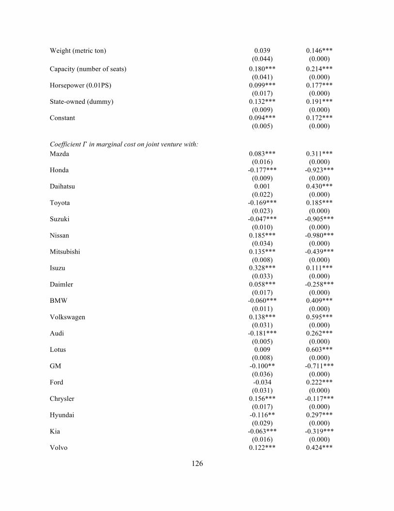
126

Weight (metric ton) 0.039 (0.044)

0.146*** (0.000)

Capacity (number of seats) 0.180*** (0.041)

0.214*** (0.000)

Horsepower (0.01PS) 0.099*** (0.017)

0.177*** (0.000)

State-owned (dummy) 0.132*** (0.009)

0.191*** (0.000)

Constant 0.094*** (0.005)

0.172*** (0.000)

Coefficient ! in marginal cost on joint venture with: Mazda 0.083***

(0.016) 0.311*** (0.000)

Honda -0.177*** (0.009)

-0.923*** (0.000)

Daihatsu 0.001 (0.022)

0.430*** (0.000)

Toyota -0.169*** (0.023)

0.185*** (0.000)

Suzuki -0.047*** (0.010)

-0.905*** (0.000)

Nissan 0.185*** (0.034)

-0.980*** (0.000)

Mitsubishi 0.135*** (0.008)

-0.439*** (0.000)

Isuzu 0.328*** (0.033)

0.111*** (0.000)

Daimler 0.058*** (0.017)

-0.258*** (0.000)

BMW -0.060*** (0.011)

0.409*** (0.000)

Volkswagen 0.138*** (0.031)

0.595*** (0.000)

Audi -0.181*** (0.005)

0.262*** (0.000)

Lotus 0.009 (0.008)

0.603*** (0.000)

GM -0.100** (0.036)

-0.711*** (0.000)

Ford -0.034 (0.031)

0.222*** (0.000)

Chrysler 0.156*** (0.017)

-0.117*** (0.000)

Hyundai -0.116** (0.029)

0.297*** (0.000)

Kia -0.063*** (0.016)

-0.319*** (0.000)

Volvo 0.122*** 0.424***

127

(0.01) (0.000) Saab 0.115***

(0.011) -0.508***

(0.000) PSA 0.136***

(0.009) -0.086***

(0.000) Fiat 0.120***

(0.026) -0.262***

(0.000) Coefficient η on quantity in marginal cost 0.002

(0.003) 0.002*** (0.000)

Estimated parameters in state-owned firms’ utility on different objectives

1ρ weight on profit 0.754*** (0.038)

0.312*** (0.021)

2ρ weight on consumer surplus 0.011 (0.009)

0.301*** (0.000)

3ρ weight on squared deviation from target number of alternative vehicles

0.006 (0.004)

0.091*** (0.000)

h target number of alternative vehicles 1050*** (0.000)

650.000*** (0.000)

# Observations 2215 2215

Notes: Standard errors are reported in parentheses. Significance codes: * p<0.05; ** p<0.01; ***p<0.001. Specification (2) is the random coefficient model and specification (3) is the traditional logit model without any interaction between consumer characteristics and product characteristics.

128

Table C3. Model including interaction with “international joint venture country” dummy allowing stated-owned firms to have different objectives, 2010-2013

(2) (3) Mean " of marginal utility of: Alternative vehicle (dummy) 0.106***

(0.000) 0.105*** (0.000)

Fuel efficiency (100km/L) 0.235*** (0.000)

0.234*** (0.000)

Length (m) 0.294*** (0.000)

0.293*** (0.005)

Weight (metric ton) 0.281*** (0.000)

0.28*** (0.002)

Capacity (number of seats) -0.133*** (0.000)

-0.134*** (0.006)

Horsepower (PS) 0.168*** (0.000)

0.167*** (0.002)

Constant 0.333*** (0.000)

0.332*** (0.001)

Standard deviation # of marginal utility of: Alternative vehicle (dummy) 0.163***

(0.000)

Fuel efficiency (100km/L) 0.112*** (0.000)

Length (m) -0.009*** (0.000)

Weight (metric ton) 0.347*** (0.000)

Capacity (number of seats) 0.105*** (0.000)

Horsepower (0.01PS) 0.029*** (0.000)

Constant 0.210*** (0.000)

Parameter $ in marginal disutility of price (1,000 Yuan) 0.420***

(0.000) 0.419*** (0.168)

Coefficient % in marginal cost on: Alternative vehicle (dummy) 0.139***

(0.000) 0.138*** (0.000)

Fuel efficiency (100km/L) 0.060*** (0.000)

0.059*** (0.000)

Length (m) 0.126*** (0.000)

0.125*** (0.000)

Weight (metric ton) 0.101*** 0.100***

129

(0.000) (0.000)

Capacity (number of seats) 0.156*** (0.000)

0.155*** (0.000)

Horsepower (0.01PS) 0.113*** (0.000)

0.112*** (0.000)

State-owned (dummy) 0.111*** (0.000)

0.110*** (0.000)

Constant 0.245*** (0.000)

0.244*** (0.000)

Coefficient ! in marginal cost on joint venture with: Mazda 0.158***

(0.000) -0.311***

(0.000) Honda -0.064***

(0.000) 0.923*** (0.000)

Daihatsu 0.054*** (0.000)

0.43*** (0.000)

Toyota 0.219*** (0.000)

0.185*** (0.000)

Suzuki -0.028*** (0.000)

-0.905*** (0.000)

Nissan 0.033*** (0.000)

0.980*** (0.000)

Mitsubishi 0.185*** (0.000)

-0.439*** (0.000)

Isuzu -0.110*** (0.000)

0.111*** (0.000)

Daimler -0.224*** (0.000)

-0.258*** (0.000)

BMW -0.059*** (0.000)

0.409*** (0.000)

Volkswagen 0.035*** (0.000)

0.595*** (0.000)

Audi 0.092*** (0.000)

0.262*** (0.000)

Lotus -0.253*** (0.000)

-0.603*** (0.000)

GM -0.189*** (0.000)

0.711*** (0.000)

Ford 0.029*** (0.000)

0.222*** (0.000)

Chrysler -0.135*** (0.000)

-0.117*** (0.000)

Hyundai 0.003*** (0.000)

-0.297*** (0.000)

Kia -0.115*** (0.000)

-0.319*** (0.000)

Volvo 0.134*** -0.424***

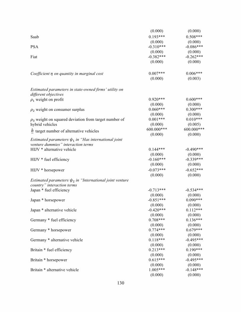
130

(0.000) (0.000) Saab 0.193***

(0.000) 0.508*** (0.000)

PSA -0.310*** (0.000)

-0.086*** (0.000)

Fiat -0.382*** (0.000)

-0.262*** (0.000)

Coefficient & on quantity in marginal cost 0.007***

(0.000) 0.006*** (0.003)

Estimated parameters in state-owned firms’ utility on different objectives

'(weight on profit 0.920*** (0.000)

0.600*** (0.000)

'*weight on consumer surplus 0.060*** (0.000)

0.300*** (0.000)

'+weight on squared deviation from target number of hybrid vehicles

0.001*** (0.000)

0.010*** (0.005)

h target number of alternative vehicles 600.000*** (0.000)

600.000*** (0.000)

Estimated parameters ,(in “Has international joint venture dummies” interaction terms

HIJV * alternative vehicle 0.144*** (0.000)

-0.490*** (0.000)

HIJV * fuel efficiency -0.160*** (0.000)

-0.339*** (0.000)

HIJV * horsepower -0.073*** (0.000)

-0.652*** (0.000)

Estimated parameters ,*in “International joint venture country” interaction terms

Japan * fuel efficiency -0.713*** (0.000)

-0.534*** (0.000)

Japan * horsepower -0.851*** (0.000)

0.090*** (0.000)

Japan * alternative vehicle -0.420*** (0.000)

0.112*** (0.000)

Germany * fuel efficiency 0.708*** (0.000)

0.136*** (0.000)

Germany * horsepower 0.774*** (0.000)

0.679*** (0.000)

Germany * alternative vehicle 0.118*** (0.000)

-0.495*** (0.000)

Britain * fuel efficiency 0.213*** (0.000)

0.190*** (0.000)

Britain * horsepower 0.615*** (0.000)

-0.495*** (0.000)

Britain * alternative vehicle 1.005*** (0.000)

-0.148*** (0.000)

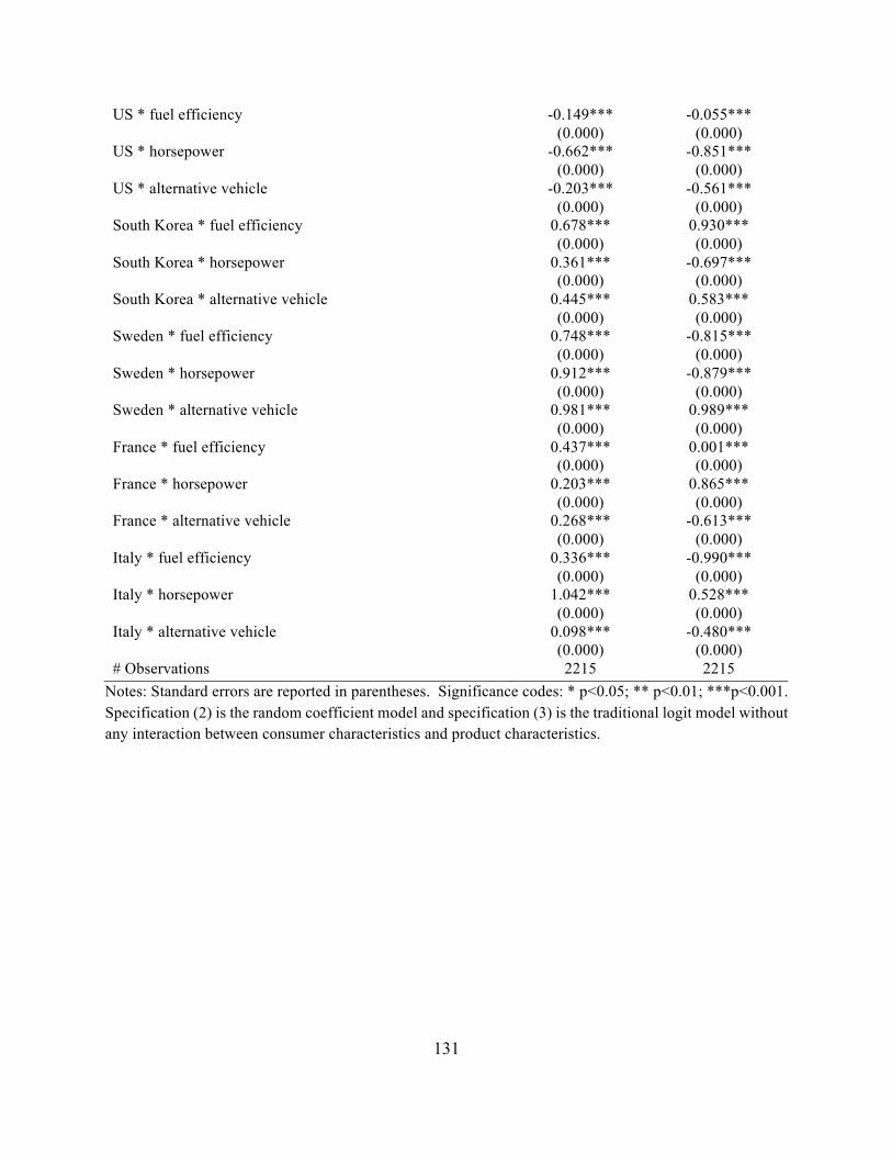
131

US * fuel efficiency -0.149*** (0.000)

-0.055*** (0.000)

US * horsepower -0.662*** (0.000)

-0.851*** (0.000)

US * alternative vehicle -0.203*** (0.000)

-0.561*** (0.000)

South Korea * fuel efficiency 0.678*** (0.000)

0.930*** (0.000)

South Korea * horsepower 0.361*** (0.000)

-0.697*** (0.000)

South Korea * alternative vehicle 0.445*** (0.000)

0.583*** (0.000)

Sweden * fuel efficiency 0.748*** (0.000)

-0.815*** (0.000)

Sweden * horsepower 0.912*** (0.000)

-0.879*** (0.000)

Sweden * alternative vehicle 0.981*** (0.000)

0.989*** (0.000)

France * fuel efficiency 0.437*** (0.000)

0.001*** (0.000)

France * horsepower 0.203*** (0.000)

0.865*** (0.000)

France * alternative vehicle 0.268*** (0.000)

-0.613*** (0.000)

Italy * fuel efficiency 0.336*** (0.000)

-0.990*** (0.000)

Italy * horsepower 1.042*** (0.000)

0.528*** (0.000)

Italy * alternative vehicle 0.098*** (0.000)

-0.480*** (0.000)

# Observations 2215 2215 Notes: Standard errors are reported in parentheses. Significance codes: * p<0.05; ** p<0.01; ***p<0.001. Specification (2) is the random coefficient model and specification (3) is the traditional logit model without any interaction between consumer characteristics and product characteristics.

132

Table C4. Model including interaction with fuel economy standard allowing stated-owned firms to have different objectives, 2010-2013 (1) (3) Mean " of marginal utility of: Alternative vehicle (dummy) 0.210***

(0.006) 0.210*** (0.000)

Fuel efficiency (100km/L) 0.211*** (0.007)

0.211*** (0.000)

Length (m) 0.017*** (0.002)

0.025*** (0.000)

Weight (metric ton) 0.220*** (0.001)

0.222*** (0.000)

Capacity (number of seats) 0.005*** (0.001)

0.014*** (0.000)

Horsepower (PS) 0.070*** (0.003)

0.072*** (0.000)

Constant 0.118*** (0.003)

0.120*** (0.000)

Standard deviation # of marginal utility of: Alternative vehicle (dummy) 0.107***

(0.006)

Fuel efficiency (100km/L) 0.133*** (0.000)

Length (m) 0.078*** (0.004)

Weight (metric ton) 0.187*** (0.002)

Capacity (number of seats) 0.065*** (0.002)

Horsepower (0.01PS) 0.046*** (0.007)

Constant 0.207*** (0.001)

Parameter $ in marginal disutility of price (1,000 Yuan) 0.348***

(0.001) 0.073*** (0.000)

Coefficient % in marginal cost on: Alternative vehicle (dummy) 0.241***

(0.008) 0.241*** (0.000)

Fuel efficiency (100km/L) 0.093*** (0.007)

0.093*** (0.000)

Length (m) 0.113*** (0.004)

0.113*** (0.000)

Weight (metric ton) 0.121*** (0.005)

0.121*** (0.000)

133

Capacity (number of seats) 0.230*** (0.006)

0.230*** (0.000)

Horsepower (0.01PS) 0.157*** (0.003)

0.157*** (0.000)

State-owned (dummy) 0.177*** (0.002)

0.177*** (0.000)

Constant 0.191*** (0.002)

0.191*** (0.000)

Coefficient ! in marginal cost on joint venture with: Mazda 0.105***

(0.005) 0.618*** (0.000)

Honda -0.085*** (0.002)

0.859*** (0.000)

Kaihatsu 0.181*** (0.003)

0.805*** (0.000)

Toyota 0.134*** (0.001)

0.577*** (0.000)

Suzuki 0.012*** (0.001)

-0.183*** (0.000)

Nissan 0.029*** (0.001)

-0.240*** (0.000)

Mitsubishi 0.012*** (0.001)

-0.887*** (0.000)

Isuzu -0.092*** (0.003)

0.029*** (0.000)

Daimler -0.237*** (0.003)

-0.490*** (0.000)

BMW -0.081*** (0.004)

-0.168*** (0.000)

Volkswagen 0.033*** (0.001)

0.979*** (0.000)

Audi 0.151*** (0.004)

-0.713*** (0.000)

Lotus -0.245*** (0.002)

0.500*** (0.000)

GM -0.225*** (0.001)

0.471*** (0.000)

Ford -0.051*** (0.010)

0.060*** (0.000)

Chrysler -0.037*** (0.008)

0.682*** (0.000)

Hyundai -0.024*** (0.001)

0.042*** (0.000)

Kia -0.159*** (0.004)

0.071*** (0.000)

Volvo 0.025*** (0.001)

0.522*** (0.000)

Saab 0.122*** 0.097***

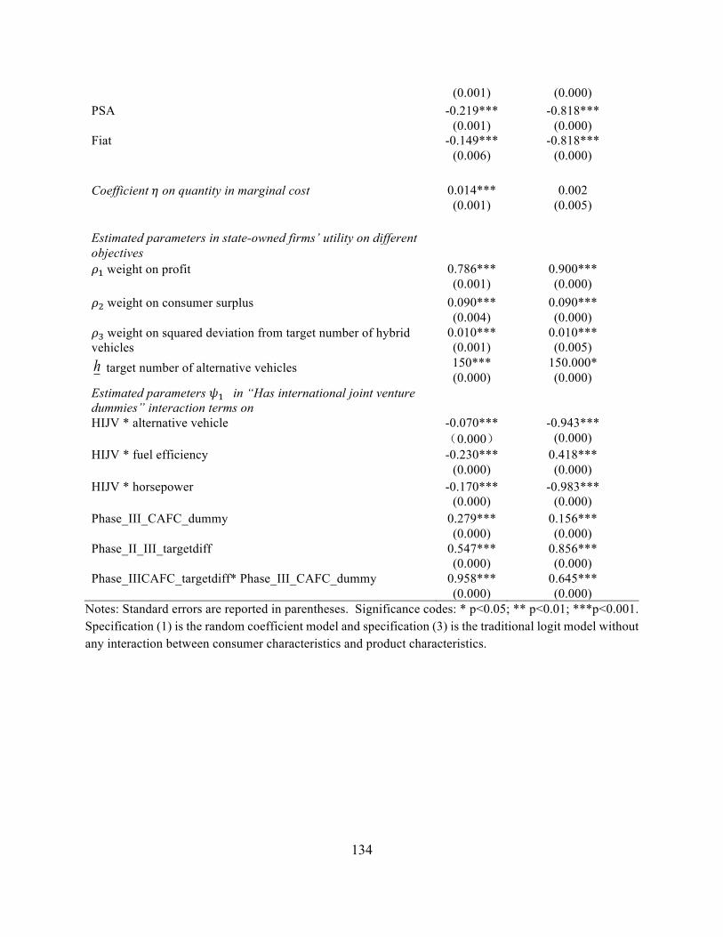
134

(0.001) (0.000) PSA -0.219***

(0.001) -0.818***

(0.000) Fiat -0.149***

(0.006) -0.818***

(0.000) Coefficient & on quantity in marginal cost 0.014***

(0.001) 0.002

(0.005) Estimated parameters in state-owned firms’ utility on different objectives

'(weight on profit 0.786*** (0.001)

0.900*** (0.000)

'*weight on consumer surplus 0.090*** (0.004)

0.090*** (0.000)

'+weight on squared deviation from target number of hybrid vehicles

0.010*** (0.001)

0.010*** (0.005)

h target number of alternative vehicles 150*** (0.000)

150.000* (0.000)

Estimated parameters ,( in “Has international joint venture dummies” interaction terms on

HIJV * alternative vehicle -0.070*** �0.000�

-0.943*** (0.000)

HIJV * fuel efficiency -0.230*** (0.000)

0.418*** (0.000)

HIJV * horsepower -0.170*** (0.000)

-0.983*** (0.000)

Phase_III_CAFC_dummy 0.279*** (0.000)

0.156*** (0.000)

Phase_II_III_targetdiff 0.547*** (0.000)

0.856*** (0.000)

Phase_IIICAFC_targetdiff* Phase_III_CAFC_dummy 0.958*** (0.000)

0.645*** (0.000)

Notes: Standard errors are reported in parentheses. Significance codes: * p<0.05; ** p<0.01; ***p<0.001. Specification (1) is the random coefficient model and specification (3) is the traditional logit model without any interaction between consumer characteristics and product characteristics.

135

Table C5. Model include interaction with fuel economy standard and interaction with “international joint venture country” dummy, possibly allowing stated-owned firms to have different objectives, 2010-2013

(2) (3) Mean " of marginal utility of: Alternative vehicle (dummy) 0.106***

(0.001) 0.105*** (0.000)

Fuel efficiency (100km/L) 0.235*** (0.002)

0.234*** (0.000)

Length (m) 0.294*** (0.004)

0.293*** (0.000)

Weight (metric ton) 0.281*** (0.001)

0.280*** (0.000)

Capacity (number of seats) -0.133*** (0.002)

0.134*** (0.000)

Horsepower (PS) 0.168*** (0.005)

0.167*** (0.000)

Constant 0.333*** (0.000)

0.332*** (0.000)

Standard deviation # of marginal utility of: Alternative vehicle (dummy) 0.163***

(0.003)

Fuel efficiency (100km/L) 0.112*** (0.001)

Length (m) -0.009 (0.007)

Weight (metric ton) 0.347*** (0.004)

Capacity (number of seats) 0.105*** (0.000)

Horsepower (0.01PS) 0.029*** (0.001)

Constant 0.210*** (0.002)

Parameter $ in marginal disutility of price (1,000 Yuan) 0.420***

(0.000) 0.419*** (0.000)

Coefficient % in marginal cost on: Alternative vehicle (dummy) 0.139***

(0.003) 0.138*** (0.000)

Fuel efficiency (100km/L) 0.060*** (0.000)

0.059*** (0.000)

Length (m) 0.126*** (0.003)

0.125*** (0.000)

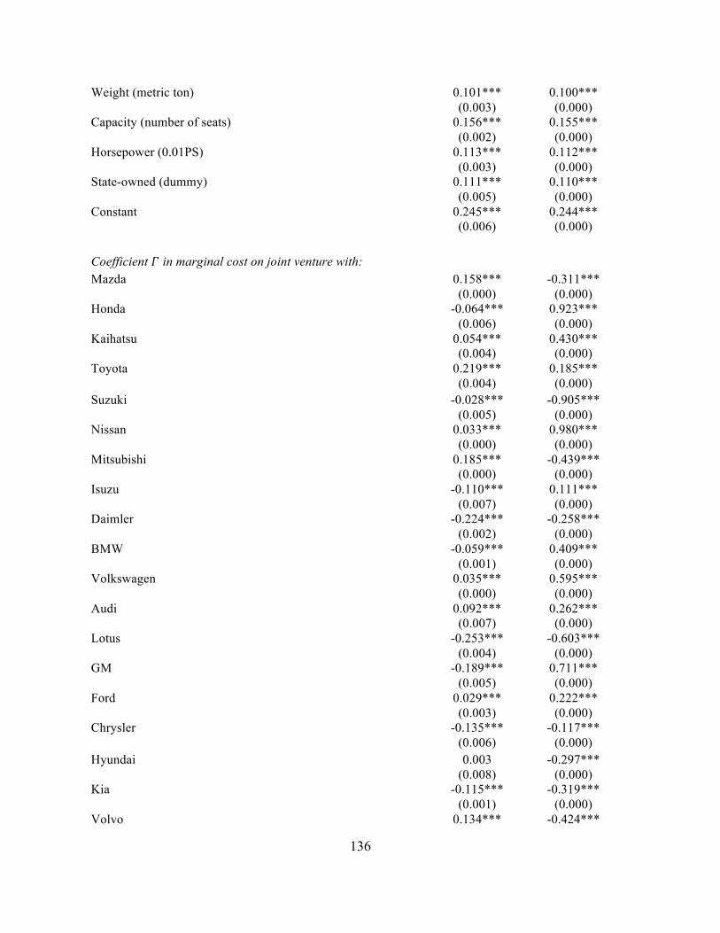
136

Weight (metric ton) 0.101*** (0.003)

0.100*** (0.000)

Capacity (number of seats) 0.156*** (0.002)

0.155*** (0.000)

Horsepower (0.01PS) 0.113*** (0.003)

0.112*** (0.000)

State-owned (dummy) 0.111*** (0.005)

0.110*** (0.000)

Constant 0.245*** (0.006)

0.244*** (0.000)

Coefficient ! in marginal cost on joint venture with: Mazda 0.158***

(0.000) -0.311***

(0.000) Honda -0.064***

(0.006) 0.923*** (0.000)

Kaihatsu 0.054*** (0.004)

0.430*** (0.000)

Toyota 0.219*** (0.004)

0.185*** (0.000)

Suzuki -0.028*** (0.005)

-0.905*** (0.000)

Nissan 0.033*** (0.000)

0.980*** (0.000)

Mitsubishi 0.185*** (0.000)

-0.439*** (0.000)

Isuzu -0.110*** (0.007)

0.111*** (0.000)

Daimler -0.224*** (0.002)

-0.258*** (0.000)

BMW -0.059*** (0.001)

0.409*** (0.000)

Volkswagen 0.035*** (0.000)

0.595*** (0.000)

Audi 0.092*** (0.007)

0.262*** (0.000)

Lotus -0.253*** (0.004)

-0.603*** (0.000)

GM -0.189*** (0.005)

0.711*** (0.000)

Ford 0.029*** (0.003)

0.222*** (0.000)

Chrysler -0.135*** (0.006)

-0.117*** (0.000)

Hyundai 0.003 (0.008)

-0.297*** (0.000)

Kia -0.115*** (0.001)

-0.319*** (0.000)

Volvo 0.134*** -0.424***

137

(0.001) (0.000) Saab 0.193***

(0.001) 0.508*** (0.000)

PSA -0.31*** (0.001)

-0.086*** (0.000)

Fiat -0.382*** (0.000)

-0.262*** (0.000)

Coefficient & on quantity in marginal cost 0.007***

(0.000) 0.006** (0.002)

Estimated parameters in state-owned firms’ utility on different objectives

'(weight on profit 0.920*** (0.002)

0.600*** (0.000)

'*weight on consumer surplus 0.060*** (0.054)

0.300*** (0.000)

'+weight on squared deviation from target number of alternative vehicles

0.001*** (0.000)

0.010* (0.005)

h target number of alternative vehicles 150*** (0.000)

600.000 (0.000)

Estimated parameters ,( in “Has international joint venture dummies” interaction terms on

HIJV * alternative vehicle 0.144*** (0.001)

-0.590*** (0.000)

HIJV * fuel efficiency -0.160*** (0.005)

-0.339*** (0.000)

HIJV * horsepower -0.073*** (0.003)

-0.650*** (0.000)

Phase_III_CAFC_dummy 0.279*** (0.003)

0.333*** (0.000)

Phase_II_III_targetdiff 0.547*** (0.004)

0.467*** (0.000)

Phase_IIICAFC_targetdiff* Phase_III_CAFC_dummy 0.958*** (0.006)

0.648*** (0.000)

Estimated parameters ,*in “International joint venture country” interaction terms

Japan * fuel efficiency -0.713*** (0.003)

0.534*** (0.000)

Japan * horsepower -0.851*** (0.002)

0.090*** (0.000)

Japan * alternative vehicle -0.420*** (0.003)

0.112*** (0.000)

Germany * fuel efficiency 0.708*** (0.002)

0.136*** (0.000)

Germany * horsepower 0.774*** (0.005)

0.679*** (0.000)

Germany * alternative vehicle 0.118*** (0.001)

-0.495*** (0.000)

138

Britain * fuel efficiency 0.213*** (0.003)

0.190*** (0.000)

Britain * horsepower 0.615*** (0.003)

-0.495*** (0.000)

Britain * alternative vehicle 1.005*** (0.002)

-0.148*** (0.000)

US * fuel efficiency -0.149*** (0.009)

-0.055*** (0.000)

US * horsepower -0.662*** (0.002)

-0.851*** (0.000)

US * alternative vehicle -0.203*** (0.002)

-0.561*** (0.000)

South Korea * fuel efficiency 0.678*** (0.002)

0.930*** (0.000)

South Korea * horsepower 0.361*** (0.001)

-0.697*** (0.000)

South Korea * alternative vehicle 0.445*** (0.002)

0.583*** (0.000)

Sweden * fuel efficiency 0.748*** (0.002)

-0.815*** (0.000)

Sweden * horsepower 0.912*** (0.001)

-0.879*** (0.000)

Sweden * alternative vehicle 0.981*** (0.004)

0.989*** (0.000)

France * fuel efficiency 0.437*** (0.002)

0.001*** (0.000)

France * horsepower 0.203*** (0.000)

0.865*** (0.000)

France * alternative vehicle 0.268*** (0.010)

-0.613*** (0.000)

Italy * fuel efficiency 0.336*** (0.002)

-0.990*** (0.000)

Italy * horsepower 1.042*** (0.000)

0.528*** (0.000)

Italy * alternative vehicle 0.098*** (0.002)

-0.480*** (0.000)

# Observations 2215 2215 Notes: Standard errors are reported in parentheses. Significance codes: * p<0.05; ** p<0.01; ***p<0.001. Specification (1) is the random coefficient model and specification (3) is the traditional logit model without any interaction between consumer characteristics and product characteristics.

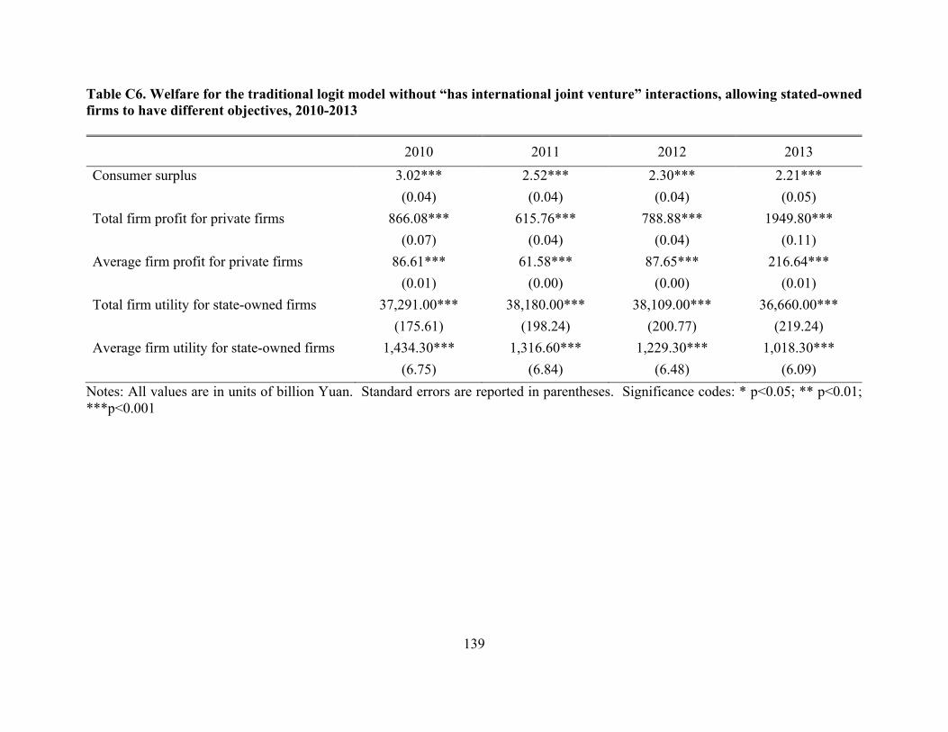
139

Table C6. Welfare for the traditional logit model without “has international joint venture” interactions, allowing stated-owned firms to have different objectives, 2010-2013 2010 2011 2012 2013

Consumer surplus 3.02*** 2.52*** 2.30*** 2.21*** (0.04) (0.04) (0.04) (0.05) Total firm profit for private firms 866.08*** 615.76*** 788.88*** 1949.80*** (0.07) (0.04) (0.04) (0.11) Average firm profit for private firms 86.61*** 61.58*** 87.65*** 216.64*** (0.01) (0.00) (0.00) (0.01) Total firm utility for state-owned firms 37,291.00*** 38,180.00*** 38,109.00*** 36,660.00*** (175.61) (198.24) (200.77) (219.24) Average firm utility for state-owned firms 1,434.30*** 1,316.60*** 1,229.30*** 1,018.30*** (6.75) (6.84) (6.48) (6.09)

Notes: All values are in units of billion Yuan. Standard errors are reported in parentheses. Significance codes: * p<0.05; ** p<0.01; ***p<0.001

140

Table C7. Welfare for the traditional logit model with “has international joint venture” interactions, allowing stated-owned firms to have different objectives, 2010-2013

2010 2011 2012 2013

Consumer surplus 2.49*** 2.01*** 1.82*** 1.742*** (0.00) (0.00) (0.00) (0.00) Total firm profit for private firms 865.99*** 615.70*** 788.84*** 1,949.60*** (3.05) (1.93) (1.69) (4.82) Average firm profit for private firms 86.60*** 61.57*** 87.65*** 216.63*** (0.31) (0.19) (0.19) (0.54) Total firm utility for state-owned firms 2,134.30*** 3,044.60*** 3,171.00*** 4,232.10*** (73.60) (79.37) (78.10) (61.90) Average firm utility for state-owned firms 82.09*** 104.99*** 102.29*** 117.56*** (2.83) (2.74) (2.52) (1.72)

Notes: All values are in units of billion Yuan. Standard errors are reported in parentheses. Significance codes: * p<0.05; ** p<0.01; ***p<0.001

141

Table C8. Welfare for the traditional logit model with international joint venture country interactions, allowing stated-owned firms to have different objectives, 2010-2013 2010 2011 2012 2013 Consumer surplus 0.00 0.00 0.00 0.00

(1.19) (0.96) (0.88) (0.85)

Total firm profit for private firms 859.65*** 611.68*** 785.32*** 1,939.60***

(3.24) (2.06) (1.80) (5.13)

Average firm profit for private firms 85.97*** 61.17*** 87.26*** 215.51***

(0.32) (0.21) (0.20) (0.57)

Total firm utility for state-owned firms 4,707.60*** 5,354.50*** 5,432.10*** 5,973.70***

(1652.00) (1677.70) (1673.00) (1580.00)

Average firm utility for state-owned firms 181.06*** 184.64*** 175.23*** 165.94*** (63.54) (57.85) (53.97) (43.89)

Notes: All values are in units of billion Yuan. Standard errors are reported in parentheses. Significance codes: * p<0.05; ** p<0.01; ***p<0.001

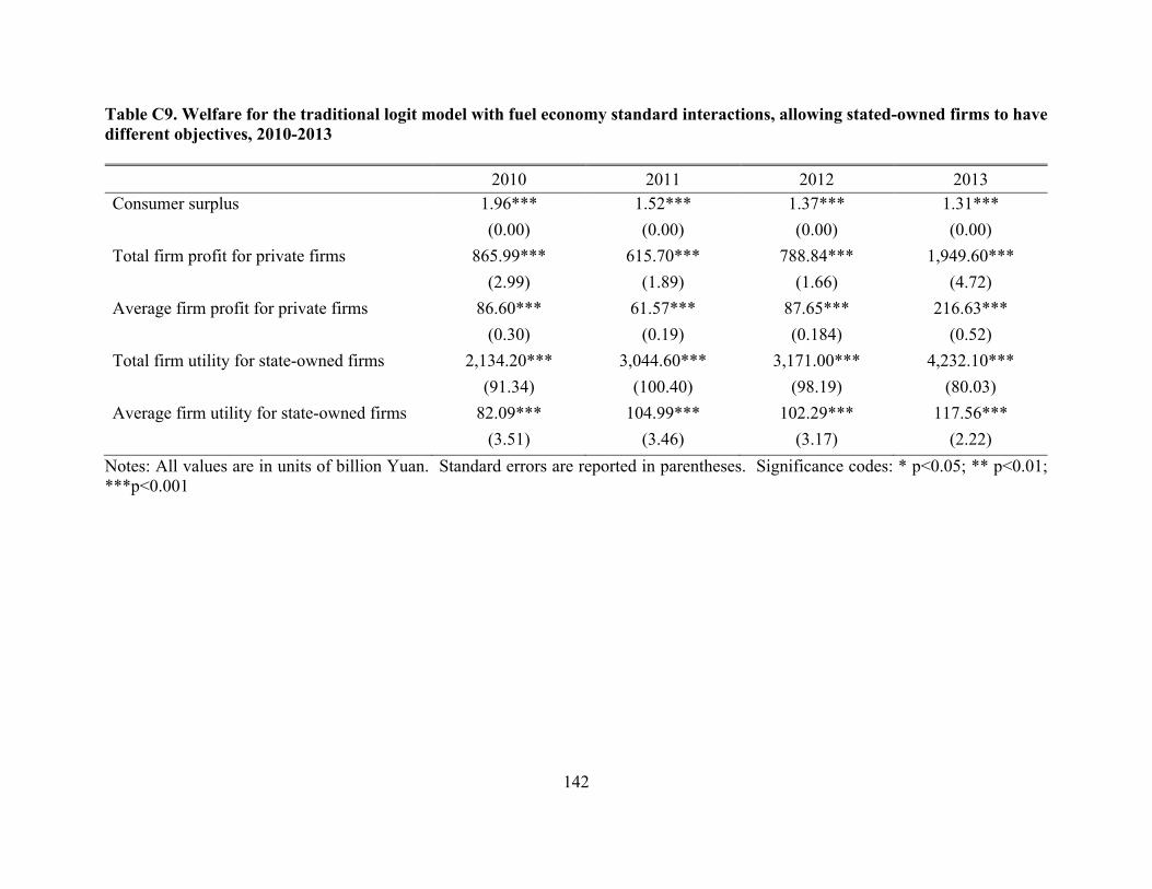
142

Table C9. Welfare for the traditional logit model with fuel economy standard interactions, allowing stated-owned firms to have different objectives, 2010-2013 2010 2011 2012 2013 Consumer surplus 1.96*** 1.52*** 1.37*** 1.31*** (0.00) (0.00) (0.00) (0.00) Total firm profit for private firms 865.99*** 615.70*** 788.84*** 1,949.60*** (2.99) (1.89) (1.66) (4.72) Average firm profit for private firms 86.60*** 61.57*** 87.65*** 216.63*** (0.30) (0.19) (0.184) (0.52) Total firm utility for state-owned firms 2,134.20*** 3,044.60*** 3,171.00*** 4,232.10*** (91.34) (100.40) (98.19) (80.03) Average firm utility for state-owned firms 82.09*** 104.99*** 102.29*** 117.56*** (3.51) (3.46) (3.17) (2.22)

Notes: All values are in units of billion Yuan. Standard errors are reported in parentheses. Significance codes: * p<0.05; ** p<0.01; ***p<0.001

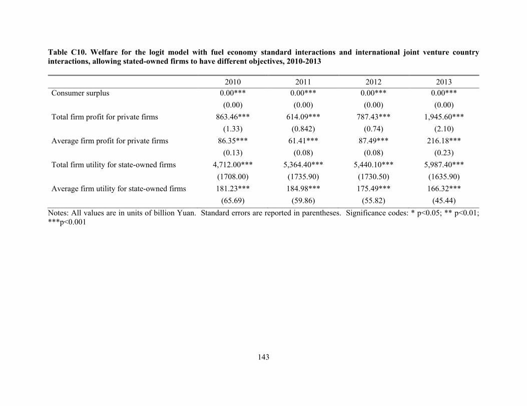
143

Table C10. Welfare for the logit model with fuel economy standard interactions and international joint venture country interactions, allowing stated-owned firms to have different objectives, 2010-2013 2010 2011 2012 2013 Consumer surplus 0.00*** 0.00*** 0.00*** 0.00*** (0.00) (0.00) (0.00) (0.00) Total firm profit for private firms 863.46*** 614.09*** 787.43*** 1,945.60*** (1.33) (0.842) (0.74) (2.10) Average firm profit for private firms 86.35*** 61.41*** 87.49*** 216.18*** (0.13) (0.08) (0.08) (0.23) Total firm utility for state-owned firms 4,712.00*** 5,364.40*** 5,440.10*** 5,987.40*** (1708.00) (1735.90) (1730.50) (1635.90) Average firm utility for state-owned firms 181.23*** 184.98*** 175.49*** 166.32*** (65.69) (59.86) (55.82) (45.44)

Notes: All values are in units of billion Yuan. Standard errors are reported in parentheses. Significance codes: * p<0.05; ** p<0.01; ***p<0.001