modeling temporal structure in music for emotion ... · p z0:t z0 qt t=1 z t;z 1 t ;; multinomial...

MODELING TEMPORAL STRUCTURE IN MUSIC FOR EMOTIONPREDICTION USING PAIRWISE COMPARISONS

Jens Madsen, Bjørn Sand Jensen, Jan LarsenTechnical University of Denmark,

Department of Applied Mathematics and Computer Science,Richard Petersens Plads, Building 321,

2800 Kongens Lyngby, Denmark{jenma,bjje,janla}@dtu.dk

ABSTRACT

The temporal structure of music is essential for the cogni-tive processes related to the emotions expressed in music.However, such temporal information is often disregardedin typical Music Information Retrieval modeling tasks ofpredicting higher-level cognitive or semantic aspects of mu-sic such as emotions, genre, and similarity. This paperaddresses the specific hypothesis whether temporal infor-mation is essential for predicting expressed emotions inmusic, as a prototypical example of a cognitive aspect ofmusic. We propose to test this hypothesis using a novel pro-cessing pipeline: 1) Extracting audio features for each trackresulting in a multivariate ”feature time series”. 2) Usinggenerative models to represent these time series (acquiringa complete track representation). Specifically, we explorethe Gaussian Mixture model, Vector Quantization, Autore-gressive model, Markov and Hidden Markov models. 3)Utilizing the generative models in a discriminative settingby selecting the Probability Product Kernel as the naturalkernel for all considered track representations. We evaluatethe representations using a kernel based model specificallyextended to support the robust two-alternative forced choiceself-report paradigm, used for eliciting expressed emotionsin music. The methods are evaluated using two data setsand show increased predictive performance using temporalinformation, thus supporting the overall hypothesis.

1. INTRODUCTION

The ability of music to represent and evoke emotions is anattractive and yet a very complex quality. This is partly aresult of the dynamic temporal structures in music, whichare a key aspect in understanding and creating predictivemodels of more complex cognitive aspects of music suchas the emotions expressed in music. So far the approach

c© Jens Madsen, Bjørn Sand Jensen, Jan Larsen.Licensed under a Creative Commons Attribution 4.0 International License(CC BY 4.0). Attribution: Jens Madsen, Bjørn Sand Jensen, Jan Larsen.“Modeling Temporal Structure in Music for Emotion Prediction usingPairwise Comparisons”, 15th International Society for Music InformationRetrieval Conference, 2014.

of creating predictive models of emotions expressed in mu-sic has relied on three major aspects. First, self-reportedannotations (rankings, ratings, comparisons, tags, etc.) forquantifying the emotions expressed in music. Secondly,finding a suitable audio representation (using audio or lyri-cal features), and finally associating the two aspects usingmachine learning methods with the aim to create predic-tive models of the annotations describing the emotions ex-pressed in music. However the audio representation hastypically relied on classic audio-feature extraction, oftenneglecting how this audio representation is later used in thepredictive models.

We propose to extend how the audio is represented byincluding feature representation as an additional aspect,which is illustrated on Figure 1. Specifically, we focus onincluding the temporal aspect of music using the added fea-ture representation [10], which is often disregarded in theclassic audio-representation approaches. In Music Informa-tion Retrieval (MIR), audio streams are often representedwith frame-based features, where the signal is divided intoframes of samples with various lengths depending on themusical aspect which is to be analyzed. Feature extractionbased on the enframed signal results in multivariate timeseries of feature values (often vectors). In order to use thesefeatures in a discriminative setting (i.e. predicting tags, emo-tion, genre, etc.), they are often represented using the mean,a single or mixtures of Gaussians (GMM). This can reducethe time series to a single vector and make the featureseasy to use in traditional linear models or kernel machinessuch as the Support Vector Machine (SVM). The majorproblem here is that this approach disregards all temporalinformation in the extracted features. The frames could berandomized and would still have the same representation,however this randomization makes no sense musically.

In modeling the emotions expressed in music, the tempo-ral aspect of emotion has been centered on how the labelsare acquired and treated, not on how the musical content istreated. E.g. in [5] they used a Conditional Random Field(CRF) model to essentially smooth the predicted labels ofan SVM, thus still not providing temporal information re-

This work was supported in part by the Danish Council for StrategicResearch of the Danish Agency for Science Technology and Innovationunder the CoSound project, case number 11-115328.

15th International Society for Music Information Retrieval Conference (ISMIR 2014)

319

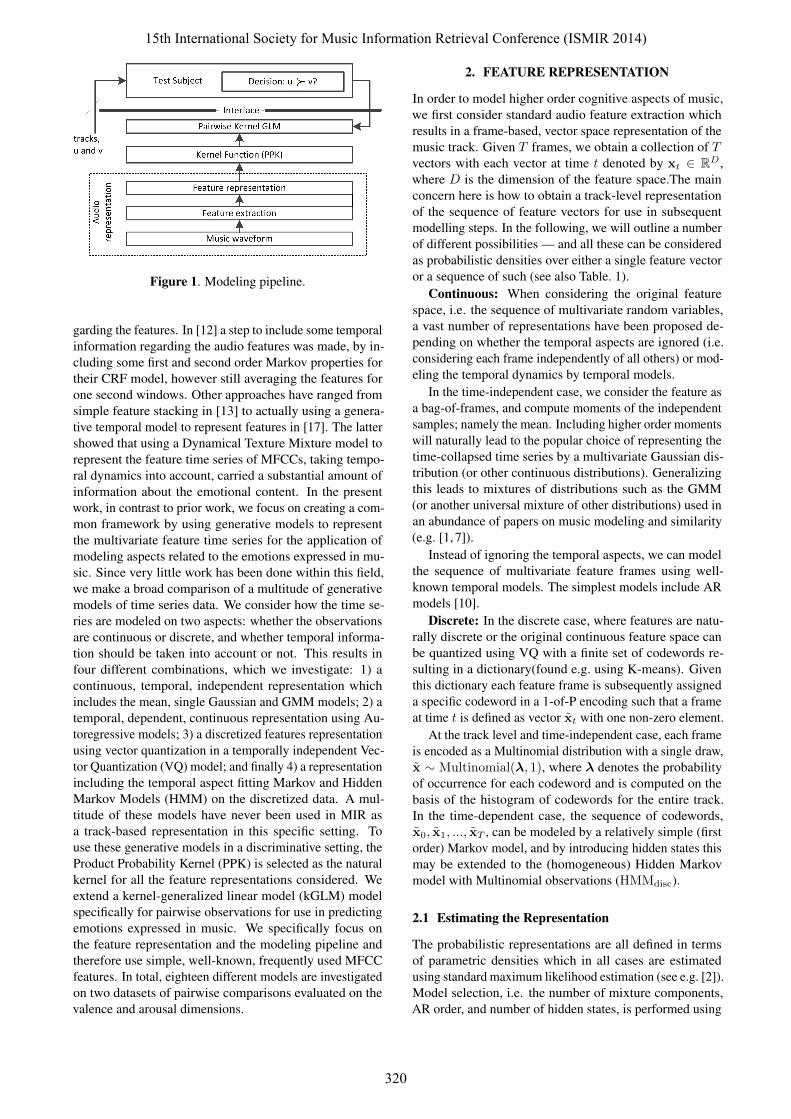
Figure 1. Modeling pipeline.

garding the features. In [12] a step to include some temporalinformation regarding the audio features was made, by in-cluding some first and second order Markov properties fortheir CRF model, however still averaging the features forone second windows. Other approaches have ranged fromsimple feature stacking in [13] to actually using a genera-tive temporal model to represent features in [17]. The lattershowed that using a Dynamical Texture Mixture model torepresent the feature time series of MFCCs, taking tempo-ral dynamics into account, carried a substantial amount ofinformation about the emotional content. In the presentwork, in contrast to prior work, we focus on creating a com-mon framework by using generative models to representthe multivariate feature time series for the application ofmodeling aspects related to the emotions expressed in mu-sic. Since very little work has been done within this field,we make a broad comparison of a multitude of generativemodels of time series data. We consider how the time se-ries are modeled on two aspects: whether the observationsare continuous or discrete, and whether temporal informa-tion should be taken into account or not. This results infour different combinations, which we investigate: 1) acontinuous, temporal, independent representation whichincludes the mean, single Gaussian and GMM models; 2) atemporal, dependent, continuous representation using Au-toregressive models; 3) a discretized features representationusing vector quantization in a temporally independent Vec-tor Quantization (VQ) model; and finally 4) a representationincluding the temporal aspect fitting Markov and HiddenMarkov Models (HMM) on the discretized data. A mul-titude of these models have never been used in MIR asa track-based representation in this specific setting. Touse these generative models in a discriminative setting, theProduct Probability Kernel (PPK) is selected as the naturalkernel for all the feature representations considered. Weextend a kernel-generalized linear model (kGLM) modelspecifically for pairwise observations for use in predictingemotions expressed in music. We specifically focus onthe feature representation and the modeling pipeline andtherefore use simple, well-known, frequently used MFCCfeatures. In total, eighteen different models are investigatedon two datasets of pairwise comparisons evaluated on thevalence and arousal dimensions.

2. FEATURE REPRESENTATION

In order to model higher order cognitive aspects of music,we first consider standard audio feature extraction whichresults in a frame-based, vector space representation of themusic track. Given T frames, we obtain a collection of Tvectors with each vector at time t denoted by xt ∈ RD,where D is the dimension of the feature space.The mainconcern here is how to obtain a track-level representationof the sequence of feature vectors for use in subsequentmodelling steps. In the following, we will outline a numberof different possibilities — and all these can be consideredas probabilistic densities over either a single feature vectoror a sequence of such (see also Table. 1).

Continuous: When considering the original featurespace, i.e. the sequence of multivariate random variables,a vast number of representations have been proposed de-pending on whether the temporal aspects are ignored (i.e.considering each frame independently of all others) or mod-eling the temporal dynamics by temporal models.

In the time-independent case, we consider the feature asa bag-of-frames, and compute moments of the independentsamples; namely the mean. Including higher order momentswill naturally lead to the popular choice of representing thetime-collapsed time series by a multivariate Gaussian dis-tribution (or other continuous distributions). Generalizingthis leads to mixtures of distributions such as the GMM(or another universal mixture of other distributions) used inan abundance of papers on music modeling and similarity(e.g. [1, 7]).

Instead of ignoring the temporal aspects, we can modelthe sequence of multivariate feature frames using well-known temporal models. The simplest models include ARmodels [10].

Discrete: In the discrete case, where features are natu-rally discrete or the original continuous feature space canbe quantized using VQ with a finite set of codewords re-sulting in a dictionary(found e.g. using K-means). Giventhis dictionary each feature frame is subsequently assigneda specific codeword in a 1-of-P encoding such that a frameat time t is defined as vector xt with one non-zero element.

At the track level and time-independent case, each frameis encoded as a Multinomial distribution with a single draw,x ∼ Multinomial(λ, 1), where λ denotes the probabilityof occurrence for each codeword and is computed on thebasis of the histogram of codewords for the entire track.In the time-dependent case, the sequence of codewords,x0, x1, ..., xT , can be modeled by a relatively simple (firstorder) Markov model, and by introducing hidden states thismay be extended to the (homogeneous) Hidden Markovmodel with Multinomial observations (HMMdisc).

2.1 Estimating the Representation

The probabilistic representations are all defined in termsof parametric densities which in all cases are estimatedusing standard maximum likelihood estimation (see e.g. [2]).Model selection, i.e. the number of mixture components,AR order, and number of hidden states, is performed using


320

Obs. Time Representation Density Model θ Base

Con

tinuo

usIndp.

Mean p (x|θ) ≡ δ (µ) µ, σ Gaussian

Gaussian p (x|θ) = N (x|µ,Σ) µ,Σ Gaussian

GMM p (x|θ) =L∑

i=1

λiN (x|µi,Σi) {λi, µi,Σi}i=1:L Gaussian

Temp. AR p (x0,x1, ..,xP |θ) = N([x0,x1, ..,xP ]

>|m,Σ|A,C

)m,Σ|A,C Gaussian

Dis

cret

e Indp. VQ p (x|θ) = λ λ Multinomial

Temp. Markov p (x0, x1, .., xT |θ) = λx0

T∏t=1

Λxt,xt−1 λ,Λ Multinomial

HMMdisc p (x0, x1, .., xT |θ) =∑z0:T

λz0

T∏t=1

Λzt,zt−1Φt λ,Λ,Φ Multinomial

Table 1. Continuous, features, x ∈ RD, L is the number of components in the GMM, P indicates the order of the ARmodel, A and C are the coefficients and noise covariance in the AR model respectively and T indicates the length of thesequence. Discrete, VQ: x ∼ Multinomial (λ), Λzt,zt−1 = p (zt|zt−1), Λxt,xt−1 = p (xt|xt−1), Φt = p (xt|zt). Thebasic Mean representation is often used in the MIR field in combination with a so-called squared exponential kernel [2],which is equivalent to formulating a PPK with a Gaussian with the given mean and a common, diagonal covariance matrixcorresponding to the length scale which can be found by cross-validation and specifically using q = 1 in the PPK.

Bayesian Information Criterion (BIC, for GMM and HMM),or in the case of the AR model, CV was used.

2.2 Kernel Function

The various track-level representations outlined above areall described in terms of a probability density as outlined inTable 1, for which a natural kernel function is the Probabil-ity Product Kernel [6]. The PPK forms a common groundfor comparison and is defined as,

k(p (x|θ) , p

(x|θ′

))=

∫ (p (x|θ) p

(x|θ′

))qdx, (1)

where q > 0 is a free model parameter. The parameters ofthe density model, θ, obviously depend on the particularrepresentation and are outlined in Tab.1. All the densitiesdiscussed previously result in (recursive) analytical compu-tations. [6, 11]. 1

3. PAIRWISE KERNEL GLM

The pairwise paradigm is a robust elicitation method to themore traditional direct scaling approach and is reviewedextensively in [8]. This paradigm requires a non-traditionalmodeling approach for which we derive a relatively simplekernel version of the Bradley-Terry-Luce model [3] forpairwise comparisons. The non-kernel version was used forthis particular task in [9].

In order to formulate the model, we will for now assumea standard vector representation for each of N audio ex-cerpts collected in the set X = {xi|i = 1, ..., N}, wherexi ∈ RD, denotes a standard, D dimensional audio fea-ture vector for excerpt i. In the pairwise paradigm, anytwo distinct excerpts with index u and v, where xu ∈ Xand xv ∈ X , can be compared in terms of a given aspect

1 It should be noted that using the PPK does not require the same lengthT of the sequences (the musical excerpts). For latent variable models,such as the HMM, the number of latent states in the models can also bedifferent. The observation space, including the dimensionality D, is theonly thing that has to be the same.

(such as arousal/valance). WithM such comparisons we de-note the output set as Y = {(ym;um, vm)|m = 1, ...,M},where ym ∈ {−1,+1} indicates which of the two excerptshad the highest valence (or arousal). ym = −1 means thatthe um’th excerpt is picked over the vm’th and visa versawhen ym = 1.

The basic assumption is that the choice, ym, between thetwo distinct excerpts, u and v, can be modeled as the differ-ence between two function values, f(xu) and f(xv). Thefunction f : X → R hereby defines an internal, but latent,absolute reference of valence (or arousal) as a function ofthe excerpt (represented by the audio features, x).

Modeling such comparisons can be accomplished by theBradley-Terry-Luce model [3, 16], here referred to moregenerally as the (logistic) pairwise GLM model. The choicemodel assumes logistically distributed noise [16] on theindividual function value, and the likelihood of observing aparticular choice, ym, for a given comparison m thereforebecomes

p (ym|fm) ≡ 1

1 + e−ym·zm, (2)

with zm = f(xum)−f(xvm

) and fm = [f(xum), f(xvm

)]T .The main question is how the function, f(·), is modeled. Inthe following, we derive a kernel version of this model in theframework of kernel Generalized Linear Models (kGLM).We start by assuming a linear and parametric model ofthe form fi = xiw

> and consider the likelihood definedin Eq. (2). The argument, zm, is now redefined such thatzm =

(xum

w> − xvmw>). We assume that the model

parameterized by w is the same for the first and second in-put, i.e. xum

and xvm. This results in a projection from the

audio features x into the dimensions of valence (or arousal)given by w, which is the same for all excerpts. Pluggingthis into the likelihood function we obtain:

p (ym|xum,xvm

,w) =1

1 + e−ym((xum−xum)w>)

. (3)


321

Following a maximum likelihood approach, the effectivecost function, ψ(·), defined as the negative log likelihoodis:

ψGLM (w) = −∑M

m=1log p (ym|xum

,xvm,w). (4)

Here we assume that the likelihood factorizes over the ob-servations, i.e. p (Y|f) =

∏Mm=1 p (ym|fm). Furthermore,

a regularized version of the model is easily formulated as

ψGLM−L2 (w) = ψGLM + γ ‖w‖22 , (5)

where the regularization parameter γ is to be found usingcross-validation, for example, as adopted here. This cost isstill continuous and is solved with a L-BFGS method.

This basic pairwise GLM model has previously beenused to model emotion in music [9]. In this work, thepairwise GLM model is extended to a general regularizedkernel formulation allowing for both linear and non-linearmodels. First, consider an unknown non-linear map of anelement x ∈ X into a Hilbert space,H, i.e., ϕ(x) : X 7→ H.Thus, the argument zm is now given as

zm = (ϕ (xum)− ϕ (xvm)) wT (6)

The representer theorem [14] states that the weights, w —despite the difference between mapped instances — can bewritten as a linear combination of the inputs such that

w =∑M

l=1αl (ϕ (xul

)− ϕ (xvl)) . (7)

Inserting this into Eq. (6) and applying the ”kernel trick” [2],i.e. exploiting that 〈ϕ (x)ϕ (x′)〉H = k (x,x′), we obtain

zm = (ϕ (xum)− ϕ (xvm))

M∑l=1

αl (ϕ(xul)− ϕ(xvl

))

=M∑l=1

αl(ϕ (xum)ϕ(xul

)− ϕ (xum)ϕ(xvl

)

− ϕ (xvm)ϕ(xul

) + ϕ (xvm)ϕ(xvl

))

=M∑l=1

αl(k (xum,xul

)− k (xum,xvl

)

− k (xvm,xul

) + k (xvm,xvl

))

=M∑l=1

αlk ({xum ,xvm}, {xul,xvl}). (8)

Thus, the pairwise kernel GLM formulation leads exactly tostandard kernel GLM like [19], where the only difference isthe kernel function which is now a (valid) kernel betweentwo sets of pairwise comparisons 2 . If the kernel functionis the linear kernel, we obtain the basic pairwise logisticregression presented in Eq. (3), but the the kernel formula-tion easily allows for non-vectorial inputs as provided bythe PPK. The general cost function for the kGLM model is

2 In the Gaussian Process setting this kernel is also known as the Pair-wise Judgment kernel [4], and can easily be applied for pairwise leaningusing other kernel machines such as support vector machines

defined as,

ψkGLM−L2 (α) = −M∑

m=1

log p (ym|α,K) + γα>Kα,

i.e., dependent on the kernel matrix, K, and parametersα. It is of the same form as for the basic model and wecan apply standard optimization techniques. Predictions forunseen input pairs {xr,xs} are easily calculated as

∆frs = f (xr)− f (xs) (9)

=∑M

m=1αm k ({xum

,xvm}, {xr,xs}). (10)

Thus, predictions exist only as delta predictions. Howeverit is easy to obtain a “true” latent (arbitrary scale) functionfor a single output by aggregating all the delta predictions.

4. DATASET & EVALUATION APPROACH

To evaluate the different feature representations, two datasetsare used. The first dataset (IMM) consists ofNIMM = 20 ex-cerpts and is described in [8]. It comprises all MIMM = 190unique pairwise comparisons of 20 different 15-secondexcerpts, chosen from the USPOP2002 3 dataset. 13 par-ticipants (3 female, 10 male) were compared on both thedimensions of valence and arousal. The second dataset(YANG) [18] consists of MYANG = 7752 pairwise compar-isons made by multiple annotators on different parts of theNYANG = 1240 different Chinese 30-second excerpts onthe dimension of valence. 20 MFCC features have beenextracted for all excerpts by the MA toolbox 4 .

4.1 Performance Evaluation

In order to evaluate the performance of the proposed repre-sentation of the multivariate feature time series we computelearning curves. We use the so-called Leave-One-Excerpt-Out cross validation, which ensures that all comparisonswith a given excerpt are left out in each fold, differing fromprevious work [9]. Each point on the learning curve isthe result of models trained on a fraction of all availablecomparisons in the training set. To obtain robust learningcurves, an average of 10-20 repetitions is used. Further-more a ’win’-based baseline (Baselow) as suggested in [8]is used. This baseline represents a model with no informa-tion from features. We use the McNemar paired test withthe Null hypothesis that two models are the same betweeneach model and the baseline, if p < 0.05 then the modelscan be rejected as equal on a 5% significance level.

5. RESULTS

We consider the pairwise classification error on the two out-lined datasets with the kGLM-L2 model, using the outlinedpairwise kernel function combined with the PPK kernel(q=1/2). For the YANG dataset a single regularization pa-rameter γ was estimated using 20-fold cross validation used

3 http://labrosa.ee.columbia.edu/projects/musicsim/uspop2002.html

4 http://www.pampalk.at/ma/


322

Obs. Time Models Training set size1% 5% 10% 20% 40% 80 % 100 %

Con

tinuo

us

Indp.

Mean 0.468 0.386 0.347 0.310 0.277 0.260 0.252N (x|µ, σ) 0.464 0.394 0.358 0.328 0.297 0.279 0.274N (x|µ,Σ) 0.440 0.366 0.328 0.295 0.259 0.253 0.246GMMdiag 0.458 0.378 0.341 0.304 0.274 0.258 0.254GMMfull 0.441 0.362 0.329 0.297 0.269 0.255 0.252

Temp.DARCV 0.447 0.360 0.316 0.283 0.251 0.235 0.228VARCV 0.457 0.354 0.316 0.286 0.265 0.251 0.248

Dis

cret

e

Indp.VQp=256 0.459 0.392 0.353 0.327 0.297 0.280 0.279*VQp=512 0.459 0.394 0.353 0.322 0.290 0.272 0.269VQp=1024 0.463 0.396 0.355 0.320 0.289 0.273 0.271

Temp.

Markovp=8 0.454 0.372 0.333 0.297 0.269 0.254 0.244Markovp=16 0.450 0.369 0.332 0.299 0.271 0.257 0.251Markovp=24 0.455 0.371 0.330 0.297 0.270 0.254 0.248Markovp=32 0.458 0.378 0.338 0.306 0.278 0.263 0.256HMMp=8 0.461 0.375 0.335 0.297 0.267 0.250 0.246HMMp=16 0.451 0.370 0.328 0.291 0.256 0.235 0.228HMMp=24 0.441 0.366 0.328 0.293 0.263 0.245 0.240HMMp=32 0.460 0.373 0.337 0.299 0.268 0.251 0.247Baseline 0.485 0.413 0.396 0.354 0.319 0.290 0.285

Table 2. Classification error on the IMM dataset applyingthe pairwise kGLM-L2 model on the valence dimension.Results are averages of 20 folds, 13 subjects and 20 rep-etitions. McNemar paired tests between each model andbaseline all result in p� 0.001 except for results markedwith * which has p > 0.05 with sample size of 4940.

across all folds in the CV. The quantization of the multi-variate time series, is performed using a standard onlineK-means algorithm [15]. Due to the inherent difficulty ofestimating the number of codewords, we choose a selectionspecifically (8, 16, 24 and 32) for the Markov and HMMmodels and (256, 512 and 1024) for the VQ models. Wecompare results between two major categories, namely withcontinuous or discretized observation space and whethertemporal information is included or not.

The results for the IMM dataset for valence are pre-sented in Table 2. For continuous observations we see aclear increase in performance between the Diagonal AR(DAR) model of up to 0.018 and 0.024, compared to tra-ditional Multivariate Gaussian and mean models respec-tively. With discretized observations, an improvement ofperformance when including temporal information is againobserved of 0.025 comparing the Markov and VQ mod-els. Increasing the complexity of the temporal represen-tation with latent states in the HMM model, an increaseof performance is again obtained of 0.016. Predicting thedimension of arousal shown on Table 3, the DAR is againthe best performing model using all training data, outper-forming the traditional temporal-independent models with0.015. For discretized data the HMM is the best performingmodel where we again see that increasing the complex-ity of the temporal representation increases the predictiveperformance. Considering the YANG dataset, the resultsare shown in Table 4. Applying the Vector AR models(VAR), a performance gain is again observed compared tothe standard representations like e.g. Gaussian or GMM.For discretized data, the temporal aspects again improvethe performance, although we do not see a clear picture thatincreasing the complexity of the temporal representationincreases the performance; the selection of the number ofhidden states could be an issue here.


Con

tinuo

us

Indp.


Temp.DARCV 0.411 0.288 0.243 0.216 0.197 0.181 0.170VARCV 0.393 0.278 0.238 0.213 0.197 0.183 0.176

Dis

cret

e

Indp.VQp=256 0.351 0.241 0.221 0.208 0.197 0.186 0.183VQp=512 0.356 0.253 0.226 0.211 0.199 0.190 0.189VQp=1024 0.360 0.268 0.240 0.219 0.200 0.191 0.190

Temp.


Table 3. Classification error on the IMM dataset applyingthe pairwise kGLM-L2 model on the arousal dimension.Results are averages of 20 folds, 13 participants and 20repetitions. McNemar paired tests between each model andbaseline all result in p� 0.001 with a sample size of 4940.


Con

tinuo

usIndp.


Temp.DARp=10 0.302 0.272 0.262 0.251 0.241 0.231 0.230VARp=4 0.281 0.260 0.249 0.236 0.223 0.210 0.206

Dis

cret

e

Indp.VQp=256 0.304 0.289 0.280 0.274 0.268 0.264 0.224VQp=512 0.303 0.286 0.276 0.269 0.261 0.254 0.253VQp=1024 0.300 0.281 0.271 0.261 0.253 0.245 0.243

Temp.


Table 4. Classification error on the YANG dataset applyingthe pairwise kGLM-L2 model on the valence dimension.Results are averages of 1240 folds and 10 repetitions. Mc-Nemar paired test between each model and baseline resultsin p� 0.001. Sample size of test was 7752.

6. DISCUSSION

In essence we are looking for a way of representing an entiretrack based on the simple features extracted. That is, we aretrying to find generative models that can capture meaningfulinformation coded in the features specifically for codingaspects related to the emotions expressed in music.

Results showed that simplifying the observation spaceusing VQ is useful when predicting the arousal data. Intro-ducing temporal coding of VQ features by simple Markovmodels already provides a significant performance gain,and adding latent dimensions (i.e. complexity) a furthergain is obtained. This performance gain can be attributedto the temporal changes in features and potentially hiddenstructures in the features not coded in each frame of the fea-tures but, by their longer term temporal structures, capturedby the models.

We see the same trend with the continuous observations,i.e. including temporal information significantly increases


323

predictive performance. These results are specific for thefeatures used, the complexity, and potentially the modelchoice might differ if other features were utilized. Futurework will reveal if other structures can be found in featuresthat describe different aspects of music; structures that arerelevant for describing and predicting aspects regardingemotions expressed in music.

Another consideration when using the generative modelsis that the entire feature time series is replaced as suchby the model, since the distances between tracks are nowbetween the models trained on each of the tracks and notdirectly on the features 5 . These models still have to beestimated, which takes time, but this can be done offlineand provide a substantial compression of the features used.

7. CONCLUSION

In this work we presented a general approach for evaluat-ing various track-level representations for music emotionprediction, focusing on the benefit of modeling temporal as-pects of music. Specifically, we considered datasets basedon robust, pairwise paradigms for which we extended aparticular kernel-based model forming a common groundfor comparing different track-level representations of mu-sic using the probability product kernel. A wide rangeof generative models for track-level representations wasconsidered on two datasets, focusing on evaluating bothusing continuous and discretized observations. Modelingboth the valence and arousal dimensions of expressed emo-tion showed a clear gain in applying temporal modelingon both the datasets included in this work. In conclusion,we have found evidence for the hypothesis that a statisti-cally significant gain is obtained in predictive performanceby representing the temporal aspect of music for emotionprediction using MFCC’s.

8. REFERENCES

[1] J-J. Aucouturier and F. Pachet. Music similarity mea-sures: What’s the use? In 3rd International Conferenceon Music Information Retrieval (ISMIR), pages 157–163, 2002.

[2] C.M. Bishop. Pattern Recognition and Machine Learn-ing. Springer, 2006.

[3] R. D. Bock and J. V. Jones. The measurement and pre-diction of judgment and choice. Holden-day, 1968.

[4] F. Huszar. A GP classification approach to preferencelearning. In NIPS Workshop on Choice Models andPreference Learning, pages 1–4, 2011.

[5] V. Imbrasaite, T. Baltrusaitis, and P. Robinson. Emotiontracking in music using continuous conditional randomfields and relative feature representation. In ICME AAMWorkshop, 2013.

[6] T. Jebara and A. Howard. Probability Product Kernels.

5 We do note that using a single model across an entire musical trackcould potentially be over simplifying the representation, in our case onlysmall 15-30-second excerpts were used and for entire tracks some segmen-tation would be appropriate.

Journal of Machine Learning Research, 5:819–844,2004.

[7] J. H. Jensen, D. P. W. Ellis, M. G. Christensen, andS. Holdt Jensen. Evaluation of distance measures be-tween gaussian mixture models of mfccs. In 8th Inter-national Conference on Music Information Retrieval(ISMIR), 2007.

[8] J. Madsen, B. S. Jensen, and J. Larsen. Predictive model-ing of expressed emotions in music using pairwise com-parisons. From Sounds to Music and Emotions, SpringerBerlin Heidelberg, pages 253–277, Jan 2013.

[9] J. Madsen, B. S. Jensen, J. Larsen, and J. B. Nielsen.Towards predicting expressed emotion in music frompairwise comparisons. In 9th Sound and Music Comput-ing Conference (SMC) Illusions, July 2012.

[10] A. Meng, P. Ahrendt, J. Larsen, and L. K. Hansen. Tem-poral feature integration for music genre classification.IEEE Transactions on Audio, Speech, and LanguageProcessing, 15(5):1654–1664, 2007.

[11] A. Meng and J. Shawe-Taylor. An investigation of fea-ture models for music genre classification using thesupport vector classifier. In International Conferenceon Music Information Retrieval, pages 604–609, 2005.

[12] E. M. Schmidt and Y. E. Kim. Modeling musical emo-tion dynamics with conditional random fields. In 12thInternational Conference on Music Information Re-trieval (ISMIR), 2011.

[13] E. M. Schmidt, J. Scott, and Y. E. Kim. Feature learn-ing in dynamic environments: Modeling the acousticstructure of musical emotion. In 13th International Con-ference on Music Information Retrieval (ISMIR), 2012.

[14] B. Scholkopf, R. Herbrich, and A. J. Smola. A gener-alized representer theorem. Computational LearningTheory, 2111:416–426, 2001.

[15] D. Sculley. Web-scale k-means clustering. InternationalWorld Wide Web Conference, pages 1177–1178, 2010.

[16] K. Train. Discrete Choice Methods with Simulation.Cambridge University Press, 2009.

[17] Y. Vaizman, R. Y. Granot, and G. Lanckriet. Modelingdynamic patterns for emotional content in music. In12th International Conference on Music InformationRetrieval (ISMIR), pages 747–752, 2011.

[18] Y-H. Yang and H.H. Chen. Ranking-Based EmotionRecognition for Music Organization and Retrieval.IEEE Transactions on Audio, Speech, and LanguageProcessing, 19(4):762–774, May 2011.

[19] J. Zhu and T. Hastie. Kernel logistic regression and theimport vector machine. In Journal of Computationaland Graphical Statistics, pages 1081–1088. MIT Press,2001.


324

modeling temporal structure in music for emotion ... · p z0:t z0 qt t=1 z t;z 1 t ;; multinomial...

Documents