modeling texas dryland cotton yields, with application...

Modeling Texas Dryland Cotton Yields, With

Application to Crop Insurance Actuarial Rating

Shu-Ling Chen and Mario J. Miranda

Texas dryland upland cotton yields have historically exhibited greater variation and more

distributional irregularities than the yields of other crops, raising concerns that

conventional parametric distribution models may generate biased or otherwise inaccurate

crop insurance premium rate estimates. Here, we formulate and estimate regime-switching

models for Texas dryland cotton yields in which the distribution of yield is conditioned on

local drought conditions. Our results indicate that drought-conditioned regime-switching

models provide a better fit to Texas county-level dryland cotton yields than conventional

parametric distribution models. They do not, however, generate significantly different

Group Risk Plan crop insurance premium rate estimates.

Key Words: actuarial rating, adverse selection, cotton, crop insurance, group risk plan,

regime-switching, yield distribution

JEL Classifications: Q10, Q14, Q18

The modeling of crop yield distributions

continues to receive considerable attention in

the academic crop insurance and agricultural

risk management literature. The importance

of properly modeling yield distributions stems

in part from the dramatic growth in partici-

pation in the U.S. crop insurance program

after the enactments of the 1994 Crop

Insurance Reform Act and the 2000 Agricul-

tural Risk Protection Act (Glauber; Goodwin,

Vandeveer, and Deal). In 2004, total coverage

under the program reached $46.6 billion, an

increase of 67% over 1998 levels.

Accurate assessment of yield distributions,

particularly their lower tails, is necessary for

precise computation of crop insurance premi-

um rates. Inaccurate rates can lead to adverse

selection, in which producers whose rates are

low relative to expected indemnities partici-

pate in greater proportion than producers

whose rates are high relative to expected

indemnities. Adverse selection raises the ratio

of indemnities paid to the premiums collected,

undermining the actuarial performance of the

federal crop insurance and reinsurance pro-

gram (Goodwin; Miranda; Skees and Reed).

Numerous studies have highlighted the

challenges associated with the statistical mod-

eling of crop yields for the rating of crop

insurance (Atwood, Shaik, and Watts; Day;

Gallagher; Goodwin and Ker; Just and

Weninger; Ker and Coble; Ker and Goodwin;

Ramirez, Misra, and Field; Sherrick et al.;

Taylor). Most published studies have devel-

oped statistical models of yields for crops and

regions in which yield variation is relatively

regular and for which crop abandonment is

Shu-Ling Chen is an assistant professor at the

Department of Quantitative Finance, National Tsing

Hua University, Taiwan and Mario J. Miranda is

Andersons Professor of Agricultural Finance and

Risk Management at the Department of Agricultural,

Environmental and Development Economics, The

Ohio State University, Columbus, OH.

The authors wish to thank Barry Goodwin, Tim

Haab, and the referees for useful comments and

suggestions.

Journal of Agricultural and Applied Economics, 40,1(April 2008):239–252# 2008 Southern Agricultural Economics Association

relatively rare (e.g., Iowa corn). In most of

these studies, standard parametric distribution

methods are applicable and the debate centers

on the appropriateness of one standard

distributional form versus another (e.g., the

normal versus the beta distribution) (Atwood,

Shaik, and Watts; Day; Gallagher; Just and

Weninger; Ramirez, Misra, and Field; Sher-

rick et al.; Taylor).

However, very little attention has been

given to the modeling of yield distributions for

crops and regions in which yields exhibit

highly irregular behavior. Of particular inter-

est are crops and regions that exhibit high

post-planting abandonment rates in years of

unfavorable weather. In such regions, near-

zero individual and aggregate yields are

observed with some frequency, making com-

mon unimodal continuous probability distri-

butions inadequate for explaining yield varia-

tion. The correct choice of distributional form

for the yields of such crops remains an

unsettled but important question.

In this paper, we undertake a statistical

case study of Texas dryland upland cotton,

which in recent years has exhibited poor

actuarial performance under the U.S. crop

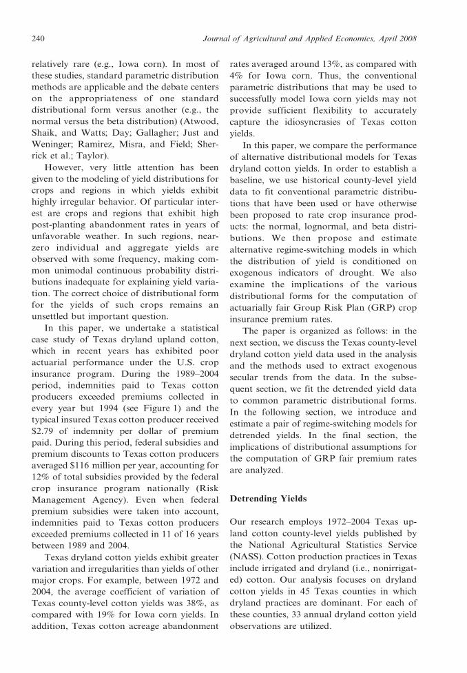
insurance program. During the 1989–2004

period, indemnities paid to Texas cotton

producers exceeded premiums collected in

every year but 1994 (see Figure 1) and the

typical insured Texas cotton producer received

$2.79 of indemnity per dollar of premium

paid. During this period, federal subsidies and

premium discounts to Texas cotton producers

averaged $116 million per year, accounting for

12% of total subsidies provided by the federal

crop insurance program nationally (Risk

Management Agency). Even when federal

premium subsidies were taken into account,

indemnities paid to Texas cotton producers

exceeded premiums collected in 11 of 16 years

between 1989 and 2004.

Texas dryland cotton yields exhibit greater

variation and irregularities than yields of other

major crops. For example, between 1972 and

2004, the average coefficient of variation of

Texas county-level cotton yields was 38%, as

compared with 19% for Iowa corn yields. In

addition, Texas cotton acreage abandonment

rates averaged around 13%, as compared with

4% for Iowa corn. Thus, the conventional

parametric distributions that may be used to

successfully model Iowa corn yields may not

provide sufficient flexibility to accurately

capture the idiosyncrasies of Texas cotton

yields.

In this paper, we compare the performance

of alternative distributional models for Texas

dryland cotton yields. In order to establish a

baseline, we use historical county-level yield

data to fit conventional parametric distribu-

tions that have been used or have otherwise

been proposed to rate crop insurance prod-

ucts: the normal, lognormal, and beta distri-

butions. We then propose and estimate

alternative regime-switching models in which

the distribution of yield is conditioned on

exogenous indicators of drought. We also

examine the implications of the various

distributional forms for the computation of

actuarially fair Group Risk Plan (GRP) crop

insurance premium rates.

The paper is organized as follows: in the

next section, we discuss the Texas county-level

dryland cotton yield data used in the analysis

and the methods used to extract exogenous

secular trends from the data. In the subse-

quent section, we fit the detrended yield data

to common parametric distributional forms.

In the following section, we introduce and

estimate a pair of regime-switching models for

detrended yields. In the final section, the

implications of distributional assumptions for

the computation of GRP fair premium rates

are analyzed.

Detrending Yields

Our research employs 1972–2004 Texas up-

land cotton county-level yields published by

the National Agricultural Statistics Service

(NASS). Cotton production practices in Texas

include irrigated and dryland (i.e., nonirrigat-

ed) cotton. Our analysis focuses on dryland

cotton yields in 45 Texas counties in which

dryland practices are dominant. For each of

these counties, 33 annual dryland cotton yield

observations are utilized.

240 Journal of Agricultural and Applied Economics, April 2008

Secular trends in yields due to exogenous

technical change pose a challenge for the

modeling of yield distributions and for the

rating of crop insurance products (Goodwin

and Mahul; Ker and Coble; Ker and Goodwin;

Ozaki et al.). Lack of sufficient data compounds

the problem, raising uncertainty about the exact

form of the trend and the yield distribution

(Goodwin and Mahul; Ozaki et al.).

We initially considered several detrending

methods suggested in literature, including first-

and higher-ordered polynomials (Atwood,

Shaik, and Watts; Goodwin and Mahul; Ozaki

et al.; Sherrick et al.) and autoregressive

integrated moving average models (Goodwin

and Ker; Ker and Goodwin). However, none

of these methods proved satisfactory, due

primarily to overfitting problems.

For the purposes of this study, we elected to

use a bi-linear spline to model yields trends. In

general, this detrending method generates

higher R2 goodness-of-fit measures than the

aforementioned methods. The bi-linear spline

model allows up to two distinct linear trends in

the data. In particular, the trend yield in period

t, yt, is presumed to be a function of time:

^yt~f tð Þ~y�zb1 min 0, t{t�ð Þz b2 max 0, t{t�ð Þ:

The breakpoint t* between linear segments and

the slopes b1 and b2 of the linear segments are

endogenously determined and estimated by

nonlinear least squares. The bi-linear spline

model appeared to be free of the overfitting

problems exhibited by more flexible models,

but provided a necessary additional degree of

flexibility not offered by a simple linear trend

model. In this analysis, the breakpoint year for

most counties occurs in the late 1980s.

Given the trend yields implied by the bi-

linear spline model, detrended county-level

Texas dryland cotton yields were computed by

normalizing observed yields to 2004 equiva-

lents as follows:

ð2Þ ydt ~yt|

^y2004

yt:

Here, ytd is the detrended yield in year t, yt is

the yield realized in year t and yt is the fitted

trend yield in year t.

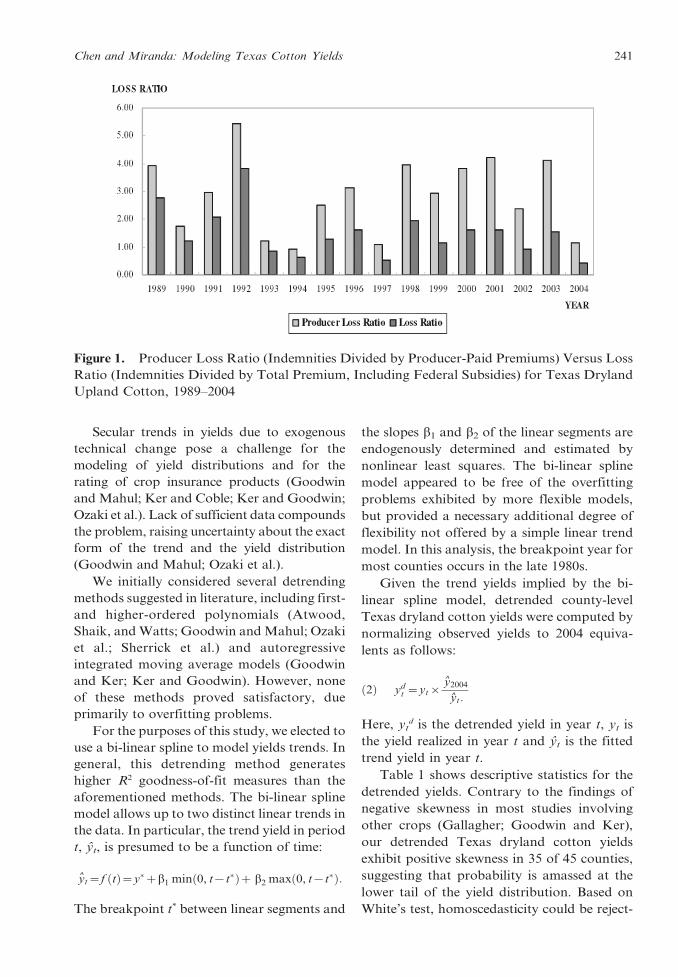
Table 1 shows descriptive statistics for the

detrended yields. Contrary to the findings of

negative skewness in most studies involving

other crops (Gallagher; Goodwin and Ker),

our detrended Texas dryland cotton yields

exhibit positive skewness in 35 of 45 counties,

suggesting that probability is amassed at the

lower tail of the yield distribution. Based on

White’s test, homoscedasticity could be reject-

Figure 1. Producer Loss Ratio (Indemnities Divided by Producer-Paid Premiums) Versus Loss

Ratio (Indemnities Divided by Total Premium, Including Federal Subsidies) for Texas Dryland

Upland Cotton, 1989–2004

Chen and Miranda: Modeling Texas Cotton Yields 241

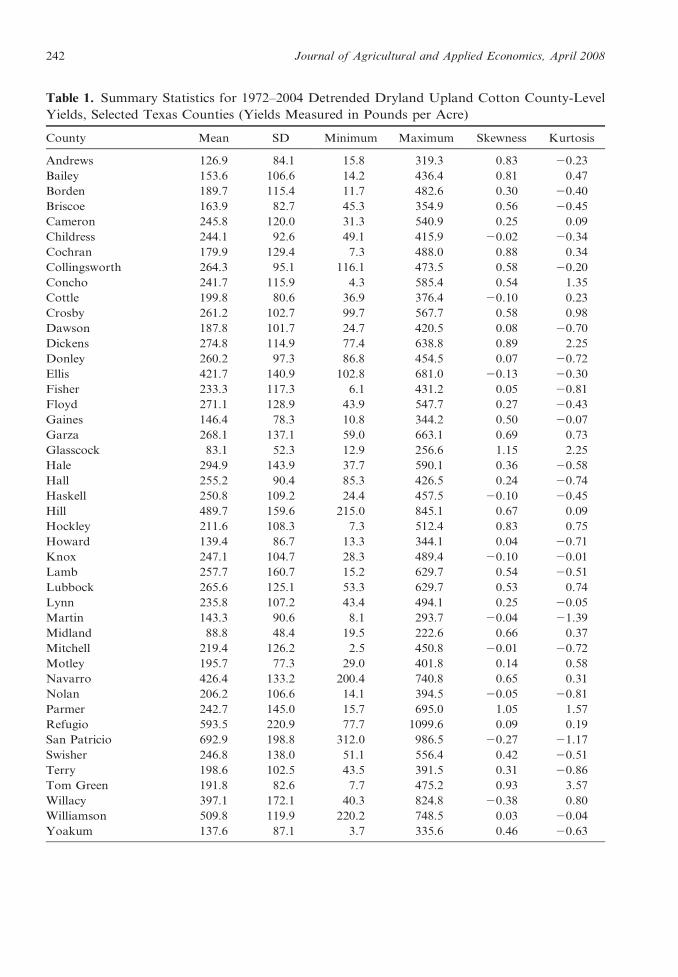
Table 1. Summary Statistics for 1972–2004 Detrended Dryland Upland Cotton County-Level

Yields, Selected Texas Counties (Yields Measured in Pounds per Acre)

County Mean SD Minimum Maximum Skewness Kurtosis

Andrews 126.9 84.1 15.8 319.3 0.83 20.23

Bailey 153.6 106.6 14.2 436.4 0.81 0.47

Borden 189.7 115.4 11.7 482.6 0.30 20.40

Briscoe 163.9 82.7 45.3 354.9 0.56 20.45

Cameron 245.8 120.0 31.3 540.9 0.25 0.09

Childress 244.1 92.6 49.1 415.9 20.02 20.34

Cochran 179.9 129.4 7.3 488.0 0.88 0.34

Collingsworth 264.3 95.1 116.1 473.5 0.58 20.20

Concho 241.7 115.9 4.3 585.4 0.54 1.35

Cottle 199.8 80.6 36.9 376.4 20.10 0.23

Crosby 261.2 102.7 99.7 567.7 0.58 0.98

Dawson 187.8 101.7 24.7 420.5 0.08 20.70

Dickens 274.8 114.9 77.4 638.8 0.89 2.25

Donley 260.2 97.3 86.8 454.5 0.07 20.72

Ellis 421.7 140.9 102.8 681.0 20.13 20.30

Fisher 233.3 117.3 6.1 431.2 0.05 20.81

Floyd 271.1 128.9 43.9 547.7 0.27 20.43

Gaines 146.4 78.3 10.8 344.2 0.50 20.07

Garza 268.1 137.1 59.0 663.1 0.69 0.73

Glasscock 83.1 52.3 12.9 256.6 1.15 2.25

Hale 294.9 143.9 37.7 590.1 0.36 20.58

Hall 255.2 90.4 85.3 426.5 0.24 20.74

Haskell 250.8 109.2 24.4 457.5 20.10 20.45

Hill 489.7 159.6 215.0 845.1 0.67 0.09

Hockley 211.6 108.3 7.3 512.4 0.83 0.75

Howard 139.4 86.7 13.3 344.1 0.04 20.71

Knox 247.1 104.7 28.3 489.4 20.10 20.01

Lamb 257.7 160.7 15.2 629.7 0.54 20.51

Lubbock 265.6 125.1 53.3 629.7 0.53 0.74

Lynn 235.8 107.2 43.4 494.1 0.25 20.05

Martin 143.3 90.6 8.1 293.7 20.04 21.39

Midland 88.8 48.4 19.5 222.6 0.66 0.37

Mitchell 219.4 126.2 2.5 450.8 20.01 20.72

Motley 195.7 77.3 29.0 401.8 0.14 0.58

Navarro 426.4 133.2 200.4 740.8 0.65 0.31

Nolan 206.2 106.6 14.1 394.5 20.05 20.81

Parmer 242.7 145.0 15.7 695.0 1.05 1.57

Refugio 593.5 220.9 77.7 1099.6 0.09 0.19

San Patricio 692.9 198.8 312.0 986.5 20.27 21.17

Swisher 246.8 138.0 51.1 556.4 0.42 20.51

Terry 198.6 102.5 43.5 391.5 0.31 20.86

Tom Green 191.8 82.6 7.7 475.2 0.93 3.57

Willacy 397.1 172.1 40.3 824.8 20.38 0.80

Williamson 509.8 119.9 220.2 748.5 0.03 20.04

Yoakum 137.6 87.1 3.7 335.6 0.46 20.63


ed at a 5% significance level in only 6 of the 45

counties, indicating that heteroscedasticity is

not a concern.

Parametric Distribution Models

In order to establish a baseline against which

to evaluate the effectiveness of alternative

distribution models for Texas county-level

dryland cotton yields, we begin by fitting

common parametric distributions to the de-

trended county-level yields. The three para-

metric distributions examined are the normal,

lognormal, and beta distributions.

Common parametric distributions often

present problems for the modeling of yield

distributions and in the rating of crop

insurance products. The beta distribution,

for example, is very sensitive to assumptions

about the maximum and minimum possible

yield, often producing unreasonable ‘‘U-

shapes’’ when the data exhibits substantial

variation (Goodwin and Mahul; Ker and

Coble). The lognormal distribution is often

criticized for possessing positive skewness, a

property generally believed not be exhibited

by yield distributions.

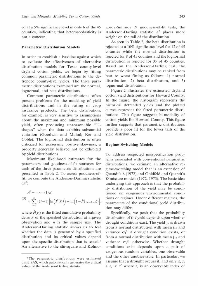
Maximum likelihood estimates for the

parameters and goodness-of-fit statistics for

each of the three parametric distributions are

presented in Table 2. To assess goodness-of-

fit, we compute the Anderson-Darling statistic

(A2):

ð3ÞA2~{n{ 1=nð Þ

|Xn

i~1

2i{1ð Þ ln F^ yið Þ

� �z ln 1{F

^ynz1{ið ÞÞ

� i,

h

where F(yi) is the fitted cumulative probability

density of the specified distribution at a given

observation and n is the sample size. The

Anderson-Darling statistic allows us to test

whether the data is generated by a specified

distribution and its critical values depend

upon the specific distribution that is tested.1

An alternative to the chi-square and Kolmo-

gorov-Smirnov D goodness-of-fit tests, the

Anderson-Darling statistic A2 places more

weight on the tail of the distribution.

As seen in Table 2, the beta distribution is

rejected at a 10% significance level for 12 of 45

counties while the normal distribution is

rejected for 8 of 45 counties and the lognormal

distribution is rejected for 35 of 45 counties.

Based on the Anderson-Darling test, the

parametric distributions may be ranked from

best to worst fitting as follows: 1) normal

distribution, 2) beta distribution, and 3)

lognormal distribution.

Figure 2 illustrates the estimated dryland

cotton yield distributions for Howard County.

In the figure, the histogram represents the

historical detrended yields and the plotted

curves represent the fitted parametric distri-

butions. This figure suggests bi-modality of

cotton yields for Howard County. This figure

further suggests that parametric distributions

provide a poor fit for the lower tails of the

yield distribution.

Regime-Switching Models

To address suspected misspecification prob-

lems associated with conventional parametric

distributions, we estimate an alternative re-

gime-switching model that is an extension of

Quandt’s l (1972) and Goldfeld and Quandt’s

D mixture models (1972, 1973). The basic idea

underlying this approach is that the probabil-

ity distribution of the yield may be condi-

tioned on exogenous environmental condi-

tions or regimes. Under different regimes, the

parameters of the conditional yield distribu-

tion may differ.

Specifically, we posit that the probability

distribution of the yield depends upon whether

drought conditions exist. The yield yt is drawn

from a normal distribution with mean m1 and

variance s12 if drought condition exists, or

from a normal distribution with mean m2 and

variance s22, otherwise. Whether drought

conditions exist depends upon a pair of

exogenous random variables, one observable

and the other unobservable. In particular, we

assume that a drought occurs if, and only if, zt

+ et , z* where zt is an observable index of

1 The parametric distributions were estimated

using SAS, which automatically generates the critical

values of the Anderson-Darling statistic.


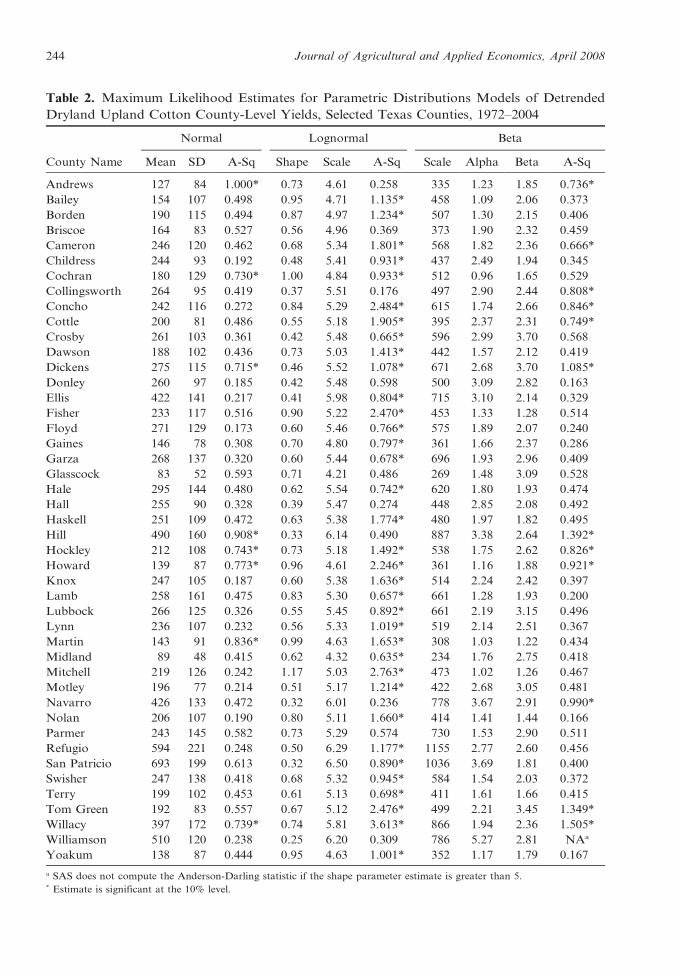
Table 2. Maximum Likelihood Estimates for Parametric Distributions Models of Detrended

Dryland Upland Cotton County-Level Yields, Selected Texas Counties, 1972–2004

County Name

Normal Lognormal Beta

Mean SD A-Sq Shape Scale A-Sq Scale Alpha Beta A-Sq

Andrews 127 84 1.000* 0.73 4.61 0.258 335 1.23 1.85 0.736*

Bailey 154 107 0.498 0.95 4.71 1.135* 458 1.09 2.06 0.373

Borden 190 115 0.494 0.87 4.97 1.234* 507 1.30 2.15 0.406

Briscoe 164 83 0.527 0.56 4.96 0.369 373 1.90 2.32 0.459

Cameron 246 120 0.462 0.68 5.34 1.801* 568 1.82 2.36 0.666*

Childress 244 93 0.192 0.48 5.41 0.931* 437 2.49 1.94 0.345

Cochran 180 129 0.730* 1.00 4.84 0.933* 512 0.96 1.65 0.529

Collingsworth 264 95 0.419 0.37 5.51 0.176 497 2.90 2.44 0.808*

Concho 242 116 0.272 0.84 5.29 2.484* 615 1.74 2.66 0.846*

Cottle 200 81 0.486 0.55 5.18 1.905* 395 2.37 2.31 0.749*

Crosby 261 103 0.361 0.42 5.48 0.665* 596 2.99 3.70 0.568

Dawson 188 102 0.436 0.73 5.03 1.413* 442 1.57 2.12 0.419

Dickens 275 115 0.715* 0.46 5.52 1.078* 671 2.68 3.70 1.085*

Donley 260 97 0.185 0.42 5.48 0.598 500 3.09 2.82 0.163

Ellis 422 141 0.217 0.41 5.98 0.804* 715 3.10 2.14 0.329

Fisher 233 117 0.516 0.90 5.22 2.470* 453 1.33 1.28 0.514

Floyd 271 129 0.173 0.60 5.46 0.766* 575 1.89 2.07 0.240

Gaines 146 78 0.308 0.70 4.80 0.797* 361 1.66 2.37 0.286

Garza 268 137 0.320 0.60 5.44 0.678* 696 1.93 2.96 0.409

Glasscock 83 52 0.593 0.71 4.21 0.486 269 1.48 3.09 0.528

Hale 295 144 0.480 0.62 5.54 0.742* 620 1.80 1.93 0.474

Hall 255 90 0.328 0.39 5.47 0.274 448 2.85 2.08 0.492

Haskell 251 109 0.472 0.63 5.38 1.774* 480 1.97 1.82 0.495

Hill 490 160 0.908* 0.33 6.14 0.490 887 3.38 2.64 1.392*

Hockley 212 108 0.743* 0.73 5.18 1.492* 538 1.75 2.62 0.826*

Howard 139 87 0.773* 0.96 4.61 2.246* 361 1.16 1.88 0.921*

Knox 247 105 0.187 0.60 5.38 1.636* 514 2.24 2.42 0.397

Lamb 258 161 0.475 0.83 5.30 0.657* 661 1.28 1.93 0.200

Lubbock 266 125 0.326 0.55 5.45 0.892* 661 2.19 3.15 0.496

Lynn 236 107 0.232 0.56 5.33 1.019* 519 2.14 2.51 0.367

Martin 143 91 0.836* 0.99 4.63 1.653* 308 1.03 1.22 0.434

Midland 89 48 0.415 0.62 4.32 0.635* 234 1.76 2.75 0.418

Mitchell 219 126 0.242 1.17 5.03 2.763* 473 1.02 1.26 0.467

Motley 196 77 0.214 0.51 5.17 1.214* 422 2.68 3.05 0.481

Navarro 426 133 0.472 0.32 6.01 0.236 778 3.67 2.91 0.990*

Nolan 206 107 0.190 0.80 5.11 1.660* 414 1.41 1.44 0.166

Parmer 243 145 0.582 0.73 5.29 0.574 730 1.53 2.90 0.511

Refugio 594 221 0.248 0.50 6.29 1.177* 1155 2.77 2.60 0.456

San Patricio 693 199 0.613 0.32 6.50 0.890* 1036 3.69 1.81 0.400

Swisher 247 138 0.418 0.68 5.32 0.945* 584 1.54 2.03 0.372

Terry 199 102 0.453 0.61 5.13 0.698* 411 1.61 1.66 0.415

Tom Green 192 83 0.557 0.67 5.12 2.476* 499 2.21 3.45 1.349*

Willacy 397 172 0.739* 0.74 5.81 3.613* 866 1.94 2.36 1.505*

Williamson 510 120 0.238 0.25 6.20 0.309 786 5.27 2.81 NAa

Yoakum 138 87 0.444 0.95 4.63 1.001* 352 1.17 1.79 0.167

a SAS does not compute the Anderson-Darling statistic if the shape parameter estimate is greater than 5.* Estimate is significant at the 10% level.


drought conditions during the critical month

of the growing season, z* is an unknown

critical threshold to be estimated, and et is an

unobserved error term, assumed to be an i.i.d.

normal random variable with zero mean and

variance s2~ee .

Under this assumption, the log likelihood

of observing yield yt in year t, conditional on

contemporaneously observed drought index zt,

is

ð4Þ

l m1,m2,s21,s2

2,z�,s~ee yt,ztj� �

~XT

t~1

log F z�{zt; 0,s~eeð Þf yt; m1,s21

� ��

zF zt{z�; 0,s~eeð Þf yt; m2,s22

� �,

where F and f are, respectively, the cumulative

distribution function and the probability den-

sity function of a standard normal variable.

We consider two alternative indices of

drought conditions, both of which are pub-

lished by the National Climatic Data Center

(NCDC): 1) average rainfall throughout the

climate division in which the county is located

and 2) the Palmer Drought Severity Index for

the climate division in which the county is

located. In all cases, the values of the indices

during the critical third month of the cotton

growing season are used to assess drought

conditions. Since the month in which cotton is

planted in Texas varies across geographic

region, ranging from February in South Texas

to June in the Plains Region, the critical third

month depends upon where the county is

located.

A challenge arises in computing estimates

for the regime switching model due to the high

irregularity of the likelihood function. In order

to rule out globally suboptimal local optima,

an extensive grid search was conducted in both

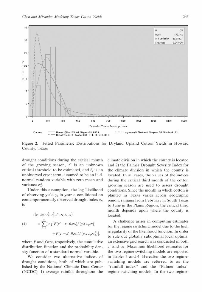
z* and se. Maximum likelihood estimates for

the two regime-switching models are reported

in Tables 3 and 4. Hereafter the two regime-

switching models are referred to as the

‘‘rainfall index’’ and the ‘‘Palmer index’’

regime-switching models. In the two regime-

Figure 2. Fitted Parametric Distributions for Dryland Upland Cotton Yields in Howard

County, Texas


Table 3. Maximum Likelihood Estimates for Rainfall Index Regime-Switching Distribution

Models of Detrended Dryland Upland Cotton County-Level Yields, Selected Texas

Counties, 1972–2004

County Name m1 m2 s1 s2 z* sE Likelihood Ratio

Andrews 71 158 30 86 1.71 0.44 17.04*

Bailey 61 178 30 104 1.13 0.78 7.78

Borden 77 267 43 75 1.38 1.22 17.04*

Briscoe 100 203 32 77 1.71 1.31 9.57*

Cameron 188 284 118 102 1.75 0.11 5.03

Childress 139 276 60 74 0.80 0.13 14.08*

Cochran 104 251 62 131 2.15 2.21 6.73

Collingsworth 190 313 46 84 1.38 0.62 11.61*

Concho 203 294 78 132 3.27 0.19 9.01*

Cottle 98 230 54 58 0.80 0.18 17.18*

Crosby 142 290 30 91 1.13 0.08 21.10*

Dawson 59 226 21 81 1.13 0.76 17.73*

Dickens 201 322 80 105 1.38 0.25 10.06*

Donley 192 303 66 87 1.38 0.11 11.02*

Ellis 320 482 116 113 1.49 0.08 12.24*

Fisher 168 371 74 43 3.18 2.52 9.43*

Floyd 213 327 84 136 2.15 0.16 10.65*

Gaines 104 186 59 71 2.15 0.00 11.40*

Garza 105 304 49 120 0.80 0.00 18.44*

Glasscock 41 106 18 49 1.71 1.24 9.25*

Hale 256 348 149 111 2.50 0.00 4.98

Hall 185 301 58 74 1.38 0.00 18.28*

Haskell 170 301 89 85 1.38 0.27 11.72*

Hill 315 537 70 140 1.05 0.33 11.43*

Hockley 131 232 26 110 1.13 0.13 16.30*

Howard 35 179 21 64 1.13 0.97 19.91*

Knox 134 279 90 82 0.80 0.23 9.79*

Lamb 112 295 36 156 1.13 0.43 14.44*

Lubbock 166 290 55 123 1.13 0.15 10.05*

Lynn 149 283 71 90 1.71 0.33 12.69*

Martin 39 201 19 53 1.71 1.52 26.37*

Midland 42 112 14 41 1.71 0.83 16.38*

Mitchell 186 323 117 80 3.18 0.00 9.90*

Motley 100 224 39 59 0.80 0.14 17.71*

Navarro 332 481 80 124 1.49 0.28 11.91*

Nolan 130 294 70 62 1.90 0.85 14.60*

Parmer 122 276 28 144 1.13 0.97 8.51*

Refugio 601 588 158 253 3.77 0.00 3.35

San Patricio 676 706 136 229 3.77 0.00 4.17

Swisher 69 292 14 114 1.13 1.14 14.97*

Terry 73 236 19 84 1.13 1.14 13.53*

Tom Green 178 241 55 126 4.11 0.24 12.62*

Willacy 361 447 202 91 2.54 0.00 10.83*

Williamson 434 552 58 122 1.49 0.11 12.34*

Yoakum 71 176 41 81 1.71 0.72 10.35*

* Denotes variables significant at the 5% level.


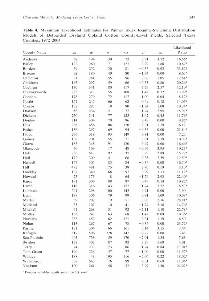
Table 4. Maximum Likelihood Estimates for Palmer Index Regime-Switching Distribution

Models of Detrended Dryland Upland Cotton County-Level Yields, Selected Texas

Counties, 1972–2004

County Name m1 m2 s1 s2 z* sE

Likelihood

Ratio

Andrews 68 194 30 72 0.91 3.72 16.66*

Bailey 122 260 71 127 3.29 1.88 10.67*

Borden 59 252 30 81 20.35 0.93 33.82*

Briscoe 92 180 40 80 21.74 0.00 9.63*

Cameron 81 281 55 96 22.06 1.05 12.61*

Childress 163 297 59 66 20.35 0.80 20.26*

Cochran 130 341 80 117 3.29 2.57 12.10*

Collingsworth 225 317 55 108 1.42 0.32 13.99*

Concho 176 279 72 117 21.00 0.04 8.12*

Cottle 152 245 66 62 0.49 0.18 14.06*

Crosby 132 288 18 90 21.74 1.08 10.34*

Dawson 58 234 21 72 21.74 2.95 15.97*

Dickens 230 341 77 125 1.42 0.45 11.76*

Donley 214 304 70 96 0.49 0.00 9.85*

Ellis 266 456 106 120 22.31 1.19 6.12

Fisher 136 297 69 94 20.35 0.00 21.84*

Floyd 236 319 93 149 0.91 0.00 7.25

Gaines 108 201 55 71 0.91 1.19 10.98*

Garza 183 348 91 120 0.49 0.00 16.66*

Glasscock 40 109 17 48 20.96 3.95 10.23*

Hale 236 517 92 37 3.29 2.89 15.22*

Hall 172 309 41 68 20.35 2.59 12.59*

Haskell 167 305 83 84 20.35 0.00 16.70*

Hill 492 481 175 38 2.96 0.59 8.10*

Hockley 167 340 66 97 3.29 3.13 11.12*

Howard 23 175 8 64 21.74 2.93 22.40*

Knox 191 300 88 87 0.49 0.14 10.82*

Lamb 118 316 43 152 21.74 3.57 8.53*

Lubbock 241 298 100 143 0.91 0.00 3.90

Lynn 187 306 79 99 0.91 1.09 10.08*

Martin 39 202 19 51 20.96 2.76 28.81*

Midland 35 107 10 41 21.74 2.18 14.76*

Mitchell 41 268 31 92 22.11 1.10 22.78*

Motley 163 243 63 68 1.42 0.09 10.36*

Navarro 283 457 62 121 22.31 1.19 6.59

Nolan 113 267 67 78 20.35 0.00 23.72*

Parmer 171 304 66 161 0.14 3.15 7.44

Refugio 617 506 228 142 2.72 0.00 3.48

San Patricio 405 738 59 170 22.01 1.34 7.68

Swisher 178 402 87 92 3.29 5.68 4.01

Terry 74 233 23 86 21.74 0.84 17.01*

Tom Green 140 226 57 77 21.00 0.00 11.57*

Willacy 188 448 195 116 22.06 0.22 18.02*

Williamson 362 543 76 99 22.31 0.69 11.06*

Yoakum 100 261 56 37 3.29 1.50 22.02*

* Denotes variables significant at the 5% level.


switching models, the maximum likelihood

estimates for se are zero in some counties,

which implies the two regimes are per-

fectly discriminated by the observed index

variable.

One would expect to observe lower yields if

drought condition exists (i.e., m1 , m2).

However, the possibility that m1 exceeds m2

cannot be completely ruled out. This is the

case, for example, for Refugio County for

both regime-switching models and for Hill

County for the Palmer index regime-switching

model. In practice, a low yield can arise not

only with extreme drought but also with

extreme moisture. The critical thresholds, z*,

in the counties where m1 , m2 in Tables 3 and

4 are very high, indicating that in these

counties, yields are drawn from a distribution

associated with very high rainfall.

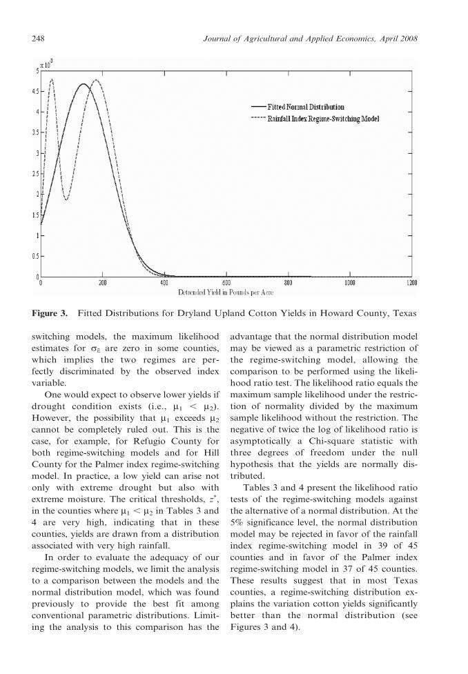
In order to evaluate the adequacy of our

regime-switching models, we limit the analysis

to a comparison between the models and the

normal distribution model, which was found

previously to provide the best fit among

conventional parametric distributions. Limit-

ing the analysis to this comparison has the

advantage that the normal distribution model

may be viewed as a parametric restriction of

the regime-switching model, allowing the

comparison to be performed using the likeli-

hood ratio test. The likelihood ratio equals the

maximum sample likelihood under the restric-

tion of normality divided by the maximum

sample likelihood without the restriction. The

negative of twice the log of likelihood ratio is

asymptotically a Chi-square statistic with

three degrees of freedom under the null

hypothesis that the yields are normally dis-

tributed.

Tables 3 and 4 present the likelihood ratio

tests of the regime-switching models against

the alternative of a normal distribution. At the

5% significance level, the normal distribution

model may be rejected in favor of the rainfall

index regime-switching model in 39 of 45

counties and in favor of the Palmer index

regime-switching model in 37 of 45 counties.

These results suggest that in most Texas

counties, a regime-switching distribution ex-

plains the variation cotton yields significantly

better than the normal distribution (see

Figures 3 and 4).

Figure 3. Fitted Distributions for Dryland Upland Cotton Yields in Howard County, Texas


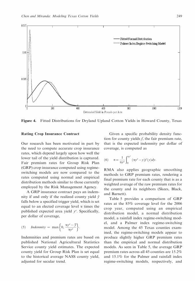
Rating Crop Insurance Contract

Our research has been motivated in part by

the need to compute accurate crop insurance

rates, which depend largely upon how well the

lower tail of the yield distribution is captured.

Fair premium rates for Group Risk Plan

(GRP) crop insurance computed using regime-

switching models are now compared to the

rates computed using normal and empirical

distribution methods similar to those currently

employed by the Risk Management Agency.

A GRP insurance contract pays an indem-

nity if and only if the realized county yield y

falls below a specified trigger yield, which is set

equal to an elected coverage level a times the

published expected area yield ye. Specifically,

per dollar of coverage,

ð5Þ Indemnity ~ max 0,aye{ ~y

aye

�:

Indemnities and premium rates are based on

published National Agricultural Statistics

Service county yield estimates. The expected

county yield for Group Risk Plan is set equal

to the historical average NASS county yield,

adjusted for secular trend.

Given a specific probability density func-

tion for county yields f, the fair premium rate,

that is the expected indemnity per dollar of

coverage, is computed as

ð6Þ p~1

aye

ðaye

0

aye{yð Þf yð Þdy:

RMA also applies geographic smoothing

methods to GRP premium rates, rendering a

final premium rate for each county that is as a

weighted average of the raw premium rates for

the county and its neighbors (Skees, Black,

and Barnett).

Table 5 provides a comparison of GRP

rates at the 85% coverage level for the 2006

crop year, computed using an empirical

distribution model, a normal distribution

model, a rainfall index regime-switching mod-

el, and a Palmer index regime-switching

model. Among the 45 Texas counties exam-

ined, the regime-switching models appear to

produce slightly higher GRP premium rates

than the empirical and normal distribution

models. As seen in Table 5, the average GRP

premium rates across all 45 counties are 15.2%

and 15.1% for the Palmer and rainfall index

regime-switching models, respectively, and

Figure 4. Fitted Distributions for Dryland Upland Cotton Yields in Howard County, Texas


Table 5. Estimated Group Risk Plan Premiums as a Percent of Liability, Texas Dryland

Upland Cotton, by County

County Name

Empirical

Distribution

Model

Normal

Distribution

Model

Palmer Regime-

Switching Model

Rainfall Regime-

Switching Model

Andrews 22.1 22.6 22.0 21.6

Bailey 23.1 24.0 21.5 24.9

Borden 22.1 20.2 27.3* 22.0

Briscoe 15.1 15.6 15.6 15.2

Cameron 14.4 14.8 18.5* 14.9

Childress 10.1 10.1 10.8 9.5

Cochran 23.9 25.2 22.7 23.8

Collingsworth 8.4 9.3 7.9 8.9

Concho 13.3 14.5 14.2 13.3

Cottle 11.3 11.1 11.4 10.8

Crosby 10.7 10.7 13.7* 11.0

Dawson 19.2 17.2 20.7 18.4

Dickens 10.3 11.8 10.6 11.7

Donley 10.5 9.9 9.4 9.8

Ellis 8.1 8.2 8.5 8.6

Fisher 15.1 15.5 15.9 16.0

Floyd 14.2 14.3 13.3 13.3

Gaines 17.1 16.9 16.0 16.8

Garza 14.7 15.8 15.7 16.7

Glasscock 20.1 21.1 21.4 22.0

Hale 14.4 14.8 14.6 15.0

Hall 9.1 9.0 9.7 9.1

Haskell 11.9 12.5 13.0 13.3

Hill 6.4 7.9* 7.3 8.2

Hockley 13.4 15.9 13.9 15.2

Howard 23.6 20.8 26.9 20.5

Knox 12.2 12.0 12.2 11.6

Lamb 21.3 20.9 21.7 21.3

Lubbock 13.9 14.1 13.5 13.7

Lynn 13.4 13.4 12.6 13.6

Martin 24.7 21.3 25.6 27.4

Midland 17.9 17.4 19.1 20.3

Mitchell 19.3 18.7 20.0 19.3

Motley 10.6 10.8 10.6 10.4

Navarro 6.3 7.3 7.5 7.0

Nolan 16.8 16.1 17.0 17.1

Parmer 18.3 19.7 17.7 20.5

Refugio 9.3 9.8 9.5 9.6

San Patricio 7.5 6.3 8.7 5.9

Swisher 17.5 18.0 16.8 24.8*

Terry 16.6 16.1 17.9 18.5

Tom Green 10.1 12.3 12.1 10.3

Willacy 12.5 12.4 12.3 12.5

Williamson 3.8 4.3 4.6 3.5

Yoakum 21.9 21.3 21.4 21.0

Average 14.6 14.7 15.2 15.1

* Indicates that the computed premium rate is statistically different from the empirical distribution premium rate at the 5%

level.


14.6% and 14.7% for the empirical and

normal distribution models, respectively.

However, the most striking feature of the

results presented by Table 5 is that there

appears to be very little difference among the

GRP premium rates computed using alterna-

tive distributional forms. In order to assess

formally whether the differences in computed

premium rates are statistically significant, we

employed nonparametric bootstrapping tech-

niques to compute estimates of the standard

errors of the differences among the various

computed premium rates. Given the estimated

standard errors, we tested the differences

between the rates generated by the empirical

distribution and the rates generated by the

normal distribution model, the rainfall index

regime-switching model, and Palmer index

regime-switching model. Of the 135 pairs of

premium rate estimates compared, only five

pairs were found to differ at the 5% level of

significance (these are indicated by an asterisk

in Table 5). Thus, we find no evidence that

regime-switching models produce GRP pre-

mium rates that are significantly different

from those computed using empirical or

normal distribution models, suggesting that

there is no compelling reason to use more

complicated regime-switching models to com-

pute Texas dryland cotton crop insurance

premium rates.

Summary and Conclusions

In this paper, we have undertaken a statistical

case study of Texas dryland cotton yields,

which historically have exhibited greater

variation and distributional irregularities than

the yields of other crops grown in other parts

of the country. As a more flexible alternative

to conventional unimodal parametric distri-

bution models, we estimated regime-switching

models in which the distribution of yield is

conditioned on local drought conditions as

measured by rainfall or the Palmer Drought

Severity Index. A comparison of the fit

provided by the various distributional forms

based on likelihood ratio and Anderson-

Darling goodness-of-fit tests indicated that

regime-switching models provide a significant-

ly better fit to observed Texas dryland cotton

yields than more conventional parametric

models.

Our findings, however, indicate that the

Group Risk Plan premium rates computed

under alternative distributional assumptions

do not systematically or significantly differ

from one another. These findings suggest that

although regime-switching models provide a

more accurate description of Texas dryland

county yield distributions than parametric

distributions overall, they possess no clear

advantage in describing the lower tail of the

distribution, which is the only portion of the

distribution that is relevant for crop insurance

actuarial ratemaking. Thus, the empirical and

normal distribution models commonly used in

actuarial ratemaking appear to provide rea-

sonable premium rate estimates and are thus

arguably preferable to the regime-switching

models examined here due to their simplicity.

[Received June 2006; Accepted August 2007.]

References

Atwood, J., S. Shaik, and M. Watts. ‘‘Are Crop

Yields Normally Distributed? A Reexamina-

tion.’’ American Journal of Agricultural Eco-

nomics 85(November 2003):888–901.

Day, R.H. ‘‘Probability Distributions of Field Crop

Yields.’’ Journal of Farm Economics 47(August

1965):713–41.

Gallagher, P. ‘‘U.S. Soybean Yields: Estimation

and Forecasting with Nonsymmetric Distur-

bances.’’ American Journal of Agricultural

Economics 69(November 1987):796–803.

Glauber, J.W. ‘‘Crop Insurance Reconsidered.’’

American Journal of Agricultural Economics

86(December 2004):1179–95.

Goldfeld, S.M., and R.E. Quandt. Nonlinear

Methods in Econometrics. Amsterdam: North-

Holland, 1972.

———.‘‘A Markov Model for Switching Regres-

sions.’’ Journal of Econometrics 1(1973):3–16.

Goodwin, B.K. ‘‘An Empirical Analysis of the

Demand for Multiple Peril Crop Insurance.’’


75(May 1993):425–34.

Goodwin, B.K., and A.P. Ker. ‘‘Nonparametric

Estimation of Crop Yield Distributions: Impli-

cations for Rating Group-Risk Crop Insurance

Contracts.’’ American Journal of Agricultural

Economics 80(February 1998):139–53.


Goodwin, B.K., and O. Mahul. ‘‘Risk Modeling

Concepts Relating to the Design and Rating of

Agricultural Insurance Contract.’’ Working

paper 3392, World Bank Policy Research,

September 2004.

Goodwin, B.K., M.L. Vandeveer, and J.L. Deal.

‘‘An Empirical Analysis of Acreage Effects of

Participation in the Federal Crop Insurance

Program.’’ American Journal of Agricultural

Economics 86(November 2004):1058–77.

Just, R.E., and Q. Weninger. ‘‘Are Crop Yields

Normally Distributed?’’ American Journal of

Agricultural Economics 81(May 1999):287–304.

Ker, A.P., and K.H. Coble. ‘‘Modeling Conditional

Yield Densities.’’ American Journal of Agricul-

tural Economics 85(May 2003):291–304.

Ker, A.P., and B.K. Goodwin. ‘‘Nonparametric

Estimation of Crop Insurance Rates Revisited.’’


82(May 2000):463–78.

Miranda, M.J. ‘‘Area-Yield Crop Insurance Re-

considered.’’ American Journal of Agricultural

Economics 73(May 1991):233–42.

National Oceanic & Atmospheric Administration

National Climatic Data Center, Internet site:

www.ncdc.noaa.gov/oa/climate/onlineprod/

drought/xmgr.html (Accessed August 30, 2007).

Ozaki, V.A., S.K. Ghosh, B.K. Goodwin, and R.

Shirota. ‘‘Spatio-Temporal Modeling of Agri-

cultural Yield Data with an Application to

Pricing Crop Insurance Contracts.’’ Paper

presented at the conference of American Agri-

cultural Economics Association Annual Meet-

ing, Providence, Rhode Island, July 24–27 2005.

Quandt, R.E. ‘‘A New Approach to Estimating

Switching Regressions.’’ Journal of the American

Statistical Association 67(June 1972):306–10.

Ramirez, O.A., S. Misra, and J. Field. ‘‘Crop-Yield

Distributions Revisited.’’ American Journal of

Agricultural Economics 85(February 2003):108–

20.

Sherrick, B.J., F.C. Zanini, G.D. Schnitkey, and

S.H. Irwin. ‘‘Crop Insurance Valuation Under

Alternative Yield Distributions.’’ American

Journal of Agricultural Economics 86(May

2004):406–19.

Skees, J.R., J.R. Black, and B.J. Barnett. ‘‘Design-

ing and Rating an Area Yield Crop Insurance

Contract.’’ American Journal of Agricultural

Economics 79(May 1997):430–38.

Skees, J.R., and M.R. Reed. ‘‘Rate Making for

Farm-Level Crop Insurance: Implication for

Adverse Selection.’’ American Journal of Agri-

cultural Economics 68(August 1986):653–59.

Taylor, C.R. ‘‘Two Practical Procedures for Esti-

mating Multivariate Nonnormal Probability

Density Functions.’’ American Journal of Agri-

cultural Economics 72(February 1990):210–17.

U.S. Department of Agriculture National Agricul-

tural Statistics Service, Internet site: www.nass.

usda.gov/index.asp (Accessed August 30, 2007).

U.S. Department of Agriculture Risk Management

Agency, Internet site: www.rma.usda.gov/ (Ac-

cessed August 30, 2007).


modeling texas dryland cotton yields, with application...

Documents