modeling the autoregressive capital asset pricing model for top 10 selected securities in bse

314

Dr. G.S. David Sam Jayakumar and W. Samuel, “Modeling The Autoregressive Capital Asset Pricing

Model For Top 10 Selected Securities In BSE” – (ICAM 2016)

MODELING THE AUTOREGRESSIVE CAPITAL ASSET PRICING MODEL

FOR TOP 10 SELECTED SECURITIES IN BSE

Dr. G.S. David Sam Jayakumar

Assistant Professor,

Jamal Institute of Management, Tiruchirappalli – 620 020

W. Samuel

Research Scholar,

Jamal Institute of Management, Tiruchirappalli – 620 020

ABSTRACT

Systematic risk is the uncertainty inherent to the entire market or entire market segment

and Unsystematic risk is the type of uncertainty that comes with the company or industry we

invest. It can be reduced through diversification. The study generalized for selecting of non -

linear capital asset pricing model for top securities in BSE and made an attempt to identify

the marketable and non-marketable risk of investors of top companies. The analysis was

conducted at different stages. They are Vector auto regression of systematic and unsystematic

risk.

Key words: Systematic Risk, Unsystematic Risk and Vector Auto Regression

Cite this Article: Dr. G.S. David Sam Jayakumar and W. Samuel. Modeling The

Autoregressive Capital Asset Pricing Model For Top 10 Selected Securities In BSE.

International Journal of Management, 7(2), 2016, pp. 314-325.

http://www.iaeme.com/ijm/index.asp

INTRODUCTION AND RELATED WORK

The capital asset pricing model (CAPM) of William Sharpe (1964) and John Lintner (1965) marks the

birth of asset pricing theory (resulting in a Nobel Prize for Sharpe in 1990). Four decades later, the

CAPM is still widely used in applications, such as estimating the cost of capital for firms and

evaluating the performance of managed portfolios. The CAPM builds on the model of portfolio choice

developed by Harry Markowitz (1959). In Markowitz’s model, an investor selects a portfolio at time t _

1 that produces a stochastic return at t. The model assumes investors are risk averse and, when

choosing among portfolios, they care only about the mean and variance of their one-period investment

return. As a result, investors choose “mean variance- efficient” portfolios, in the sense that the

portfolios The capital asset pricing model (CAPM) is used to determine a theoretically appropriate

required rate of return of an asset, if that asset is to be added to an already well-diversified portfolio,

given that asset's non- diversifiable risk. The model takes into account the asset's sensitivity to non-

diversifiable risk (also known as systematic risk or market risk, often represented by the quantity beta

INTERNATIONAL JOURNAL OF MANAGEMENT (IJM)

ISSN 0976-6502 (Print)

ISSN 0976-6510 (Online)

Volume 7, Issue 2, February (2016), pp. 314-325

http://www.iaeme.com/ijm/index.asp

Journal Impact Factor (2016): 8.1920 (Calculated by GISI)

www.jifactor.com

IJM

© I A E M E

http://www.jifactor.com/

International Journal of Management (IJM), ISSN 0976 – 6502(Print), ISSN 0976 -

6510(Online), Volume 7, Issue 2, February (2016), pp. 314-325© IAEME Publication

315



(β) in the financial industry, as well as the expected return of the market and the expected return of a

theoretical risk free asset.

The capital asset pricing model (CAPM) is the standard risk-return model used by most

academicians and practitioners. The underlying concept of CAPM is that investors are rewarded

for only that portion of risk which is not diversifiable. This non-diversifiable risk is termed as

beta, to which expected returns are linked.

It is mandatory to review the literature available with respect to the area of research study. Several

studies have been undertaken to analyze the capital asset price model. The present chapter presents

some of the studies conducted by the analysts in the past. michael c. jensen (1972) provides

Considerable attention has recently been given to general equilibrium models of the pricing of capital

assets. Of these, perhaps the best known is the mean-variance formulation originally developed by

Sharpe (1964) and Treynor (1961), and extended and clarified by Lintner (1965a; 1965b), Mossin

(1966), Fama (1968a; 1968b), and Long (1972). In addition Treynor (1965), Sharpe (1966), and Jen

sen (1968; 1969) have developed portfolio evaluation models which are either based on this asset

pricing model or bear a close relation to it. In the development of the asset pricing model it is assumed

that (1) all investors are single period risk-averse utility of terminal wealth maximizes and can choose

among portfolios solely on the basis of mean and variance, (2) there are no taxes or transactions costs,

(3) all investors have homogeneous views regarding the parameters of the joint probability distribution

of all security returns, and (4) all investors can borrow and lend at a given riskless rate of interest. The

main result of the model is a statement of the relation between the expected risk premiums on

individual assets and their "systematic risk." Our main purpose is to present some additional tests of

this asset pricing model which avoid some of the problems of earlier studies and which, we believe,

provide additional insights into the nature of the structure of security returns. The evidence presented in

Section II indicates the expected excess return on an asset is not strictly proportional to its B, and we

believe that this evidence, coupled with that given in Section IV, is sufficiently strong to warrant

rejection of the traditional form of the model given by (1). We then show in Section III how the cross-

sectional tests are subject to measurement error bias, provide a solution to this problem through

grouping procedures, and show how cross-sectional methods are relevant to testing the expanded two-

factor form of the model. We show in Section IV that the mean of the beta factor has had a positive

trend over the period 1931-65 and was on the order of 1.0 to 1.3% per month in the two sample

intervals we examined in the period 1948-65.

This seems to have been significantly different from the average risk-free rate and indeed is

roughly the same size as the average market return of 1.3 and 1.2% per month over the two sample

intervals in this period. This evidence seems to be sufficiently strong enough to warrant rejection of the

traditional form of the model given by (1). In addition, the standard deviation of the beta factor over

these two sample intervals was 2.0 and 2.2% per month, as compared with the standard deviation of the

market factor of 3.6 and 3.8% per month. Thus the beta factor seems to be an important determinant of

security returns. tim bollerslev et al(1988) examines the capital asset pricing model provides a

theoretical structure for the pricing of assets with uncertain returns. The premium to induce risk-averse

investors to bear risk is proportional to the no diversifiable risk, which is measured by the covariance

of the asset return with the market portfolio return. In this paper a multivariate generalized

autoregressive conditional heteroscedastic process is estimated for returns to bills, bonds, and stock

where the expected return is proportional to the conditional covariance of each return with that of a

fully diversified or market portfolio. It is found that the conditional covariance’s are quite variable over

time and are a significant determinant of time-varying risk premia. are also time-varying and forecast

able. However, there is evidence that other variables including innovations in consumption should also

be considered in the investor's information set when estimating the conditional distribution of returns.

viral v. acharya et al(2005) examines explicitly a simple equilibrium model with liquidity risk. In our

liquidity adjusted capital asset pricing model, a security’s required return depends on its expected

liquidity as well as on the covariance’s of its own return and liquidity with the market return and

liquidity. In addition, a persistent negative shock to a security’s liquidity results in low

contemporaneous returns and high predicted future returns. The model provides a unified framework

for understanding the various channels through which liquidity risk may affect asset prices. Our

empirical results shed light on the total and relative economic significance of these channels and

provide evidence of flight to liquidity. Peter hordahl et al(2007)



316



This paper reviews analytical work carried out by central banks that participated at the Autumn

Meeting of Central Bank Economists on “Understanding asset prices: determinants and policy

implications”, which the BIS hosted on 30–31 October 2006. The paper first discusses some general

properties of asset prices, focusing on volatilities and co-movements. It then reviews studies that look

at determinants of asset prices and that attempt to estimate a fair value of assets. The next part of the

paper focuses on research that aims at measuring the impact of changes in asset wealth on the real

economy. It then goes on to discuss how central banks use information from asset prices to develop

indicators of market expectations that are useful for monetary policy purposes. Finally, the paper

reviews central banks’ views on whether monetary policy should react in a direct way to asset price

developments. Javed iqbalet al(2007) This study investigates the applicability of the CAPM in

explaining the cross section of stock return on the Karachi Stock Exchange for the period September

1992 to April 2006. Unlike earlier studies on emerging markets this study is carried out with a broader

scope. Firstly, the tests are conducted on individual stocks as well as size sorted portfolios and industry

portfolios. Secondly, the test accounts for the intervalling affect by employing three data frequencies

namely daily, weekly and monthly data. Thirdly, keeping in view the infrequent trading prevailing in

emerging markets in general and Pakistan’s equity markets in particular the test is also carried out on

beta corrected for thin trading, using the Dimson (1979) procedure. Contrary to earlier studies on

emerging markets the premium for beta risk and the skewness have the expected signs. The risk return

relationship however appears to be non-linear and is most profound in recent years when the market

performance, backed by the high level of liquidity and trading activity, was outstanding. David e. allen

et al (2009) empirically examines the behavior of the three risk factors from Fama-French Three Factor

model of stock returns, beyond the mean of the distribution, by using quantile regressions and a US

data set. The study not only shows that the factor models does not necessarily follow a linear

relationship but also shows that the traditional method of OLS becomes less effective when it comes to

analyzing the extremes within a distribution, which is often of key interest to investors and risk

managers. John hunter et al (2009) provides a multifactor model of UK stock returns is developed,

replacing the conventional consumption habit reference by a relation that depends on US wealth two

step Instrumental Variables and Generalized Method of Moments estimators are applied to reduce the

impact of weak instruments.

The standard errors are corrected for the generated regressor problem and the model is found to

explain UK excess returns by UK consumption growth and expected US excess returns. Hence,

controlling for nominal effects by subtracting a risk free rate and conditioning on real US excess

returns provides a coherent explanation of the equity premium puzzle. Mohammad hasmat ali et

al(2010)aims to test the validity of the capital asset pricing model in the Dhaka Stock Exchange of

Bangladesh. The study period for the study covers from July 1998 to June 2008. The sample of the

study is 160 companies listed at Dhaka Stock Exchange. We attempt to investigate the relation between

risk (beta) and return by using the Fama and Macbeth (1973) approach. We find that there is a relation

between risk and return but the relation is not linear and beta cannot be considered as the main and only

source of risk. This study concludes on weak practical implication of CAPM in emerging stock

markets. It is recommended to consider other important variables to find an effective pricing

mechanism. It is also recommended to apply some other methodologies to validate the CAPM. Amit

goyal (2011) review the state of empirical asset pricing devoted\ to understanding cross sectional

differences in average rates of return.

Both methodologies and empirical evidence are surveyed. Tremendous progress has been made in

understanding return patterns. At the same time, there is a need to synthesize the huge amount of

collected evidence. S.Saravanan et al(2013) examines the CAPM is used to determine a theoretically

appropriate, required rate of return for an asset, if that asset is to be added to an already well-diversified

portfolio, given that assets have non-diversifiable risk. The model takes into account the asset’s

sensitivity to systematic risk, often represented by the quantity, beta, and the expected return of a

theoretical risk-free asset. The CAPM says that expected return of a security or a portfolio equals the

rate on a risk-free security plus a risk premium. If this expected return does not meet or beat the

required return, then the investment should not be undertaken. The security market line plots the result

of CAPM for all different risks (betas). josipa dzaja et al(2013)examines if the Capital Asset Pricing

Mo\del (CAPM) is adequate for capital asset valuation on the Central and South-East European

emerging securities markets using monthly stock returns for nine countries for the period of January

2006 to December 2010. Precisely, it is tested if beta, as the systematic risk measure, is valid on



317



observed markets by analyzing are high expected returns associated with high levels of risk, i.e. beta.

Also, the efficiency of market indices of observed countries is examined. Hamidreza vakili Fard and

Amin Babei Falah (2015) introduced a new CAPM to forecast the expected rate of return in a more

befitting manner. They first provide a brief for a development of the CAPM and its pros and cons.

Then they try and establish their new CAPM model. The main difference of their model is the use of

two betas. In the end. In the end they use the listed basic metals companies to present a practical

example of the application of the proposed model. Stefan Daniel and Josef glova (2015) explores

CAPM in its dynamic time-varying form generally applicable in determination of equity costs within

business valuation process. They briefly describe the literature on the CAPM and general index model

specifying risk premium and equity costs determination.

Their short discussion of the published literature suggests that while the CAPM is still popular

with the professional practice, its effectiveness for risk premium determination is limited. So in the

next part we shortly describe the applicability of the time-varying CAPM as an augmented approach to

the traditional CAPM form. To illustrate applicability of the model they employ this augmented

concept by incorporating only unexpected changes in the autoregressive time series models in a

specified company Dell Inc. In the final part they discuss achieved results and their possible

applicability in equity risk premium determination. Distribution fitting and simulation techniques have

been also used to provide more viable results of equity costs.

METHODOLOGY AND TECHNIQUES OF DATA ANALYSIS

For the purpose to evaluate the systematic risk and unsystematic risk of investors the authors selected

top 10 companies listed in BSE 30. The top 10 companies are Reliance industries, Bharat Heavy

Electricals limited (BHEL), Hindustan Unilever (HUL), ITC, National Thermal Power Corporation

Limited (NTPC), State Bank of India (SBI), Maruthi Suzuki, Larsen & Toubro (L & T), Tata

Consultancy services (TCS) and Tata motors. The analysis was conducted at different stages. Stage 1

Univariate Normality test of the top companies in BSE. Stage 2 Selection of maximum lag length with

security return for each company. Stage 3 Vector auto regression in CAPM of top companies in BSE.

Vector autoregression (VAR) is an econometric model used to capture the linear interdependencies

among multiple time series. VAR models generalize the univariate autoregression (AR) models by

allowing for more than one evolving variable. All variables in a VAR are treated symmetrically in a

structural sense each variable has an equation explaining its evolution based on its own lags and the

lags of the other model variables. VAR modeling does not require as much knowledge about the forces

influencing a variable as do structural models with simultaneous equations: The only prior knowledge

required is a list of variables which can be hypothesized to affect each other intertemporally.

DEFINITION

A VAR model describes the evolution of a set of k variables (called endogenous variables) over the

same sample period (t = 1, ..., T) as a linear function of only their past values. The variables are

collected in a k × 1 vector yt, which has as the i th element, yi,t, the time t observation of the i

th variable.

For example, if the i th

variable is GDP, then yi,t is the value of GDP at time t.

A p-th order VAR, denoted VAR (p), is

where the l-periods back observation yt−l is called the l-th lag of y, c is a k × 1 vector of constants

(intercepts), Ai is a time-invariant k × k matrix and et is a k × 1 vector of error terms satisfying

— every error term has mean zero;

— the contemporaneous covariance matrix of error terms is Ω (a k × k positive-

semidefinite matrix);

for any non-zero k — there is no correlation across time; in particular, no serial

correlation in individual error terms. See Hatemi-J (2004) for multivariate tests for autocorrelation in

the VAR models.

http://en.wikipedia.org/wiki/Econometric_model

http://en.wikipedia.org/wiki/Time_series

http://en.wikipedia.org/wiki/Autoregression

http://en.wikipedia.org/wiki/AR_model

http://en.wikipedia.org/wiki/Lag_operator

http://en.wikipedia.org/wiki/Structural_equation_modeling

http://en.wikipedia.org/wiki/Simultaneous_equations_model

http://en.wikipedia.org/wiki/Sample_(statistics)

http://en.wikipedia.org/wiki/Linear

http://en.wikipedia.org/wiki/Vector_space

http://en.wikipedia.org/wiki/GDP

http://en.wikipedia.org/wiki/Y-intercept

http://en.wikipedia.org/wiki/Matrix_(mathematics)

http://en.wikipedia.org/wiki/Errors_and_residuals_in_statistics

http://en.wikipedia.org/wiki/Expected_value

http://en.wikipedia.org/wiki/Covariance_matrix

http://en.wikipedia.org/wiki/Positive-definite_matrix

http://en.wikipedia.org/wiki/Positive-definite_matrix

http://en.wikipedia.org/wiki/Correlation

http://en.wikipedia.org/wiki/Serial_correlation

http://en.wikipedia.org/wiki/Serial_correlation



318



A pth-order VAR is also called a VAR with p lags. The process of choosing the maximum lag p in

the VAR model requires special attention because inference is dependent on correctness of the selected

lag order.

ORDER OF INTEGRATION OF THE VARIABLES

Note that all variables have to be of the same order of integration. The following cases are distinct:

All the variables are I(0) (stationary): one is in the standard case, i.e. a VAR in level

All the variables are I(d) (non-stationary) with d > 0

The variables are cointegrated: the error correction term has to be included in the VAR. The model

becomes a Vector error correction model (VECM) which can be seen as a restricted VAR. The

variables are not cointegrated: the variables have first to be differenced d times and one has a VAR in

difference.

CONCISE MATRIX NOTATION

One can stack the vectors in order to write a VAR (p) with a concise matrix notation:

Details of the matrices are in a separate page.

Example

For a general example of a VAR (p) with k variables, see General matrix notation of a VAR (p).

A VAR (1) in two variables can be written in matrix form (more compact notation) as

(in which only a single A matrix appears because this example has a maximum lag p equal to 1),

or, equivalently, as the following system of two equations

Each variable in the model has one equation. The current (time t) observation of each variable

depends on its own lagged values as well as on the lagged values of each other variable in the VAR.

WRITING VAR (P) AS VAR (1)

A VAR with p lags can always be equivalently rewritten as a VAR with only one lag by

appropriately redefining the dependent variable. The transformation amounts to stacking the lags of the

VAR (p) variable in the new VAR (1) dependent variable and appending identities to complete the

number of equations.

For example, the VAR (2) model

Can be recast as the VAR (1) model

Where I is the identity matrix.

http://en.wikipedia.org/wiki/Inference

http://en.wikipedia.org/wiki/Order_of_integration

http://en.wikipedia.org/wiki/Cointegration

http://en.wikipedia.org/wiki/Error_correction_model

http://en.wikipedia.org/wiki/Cointegration

http://en.wikipedia.org/wiki/General_matrix_notation_of_a_VAR(p)

http://en.wikipedia.org/wiki/General_matrix_notation_of_a_VAR(p)

http://en.wikipedia.org/wiki/Identity_matrix



319



The equivalent VAR (1) form is more convenient for analytical derivations and allows more

compact statements.

STRUCTURAL VAR

A structural VAR with p lags (sometimes abbreviated SVAR) is

where c0 is a k × 1 vector of constants, Bi is a k × k matrix (for every i = 0, ..., p) and εt is a k × 1

vector of error terms. The main diagonal terms of the B0 matrix (the coefficients on the ith

variable in

the ith equation) are scaled to 1.

The error terms εt (structural shocks) satisfy the conditions (1) - (3) in the definition above, with

the particularity that all the elements off the main diagonal of the covariance

matrix are zero. That is, the structural shocks are uncorrelated.

For example, a two variable structural VAR(1) is:

hat is, the variances of the structural shocks are denoted (i = 1, 2) and the covariance is .

Writing the first equation explicitly and passing y2,t to the right hand side one obtains

Note that y2,t can have a contemporaneous effect on y1,t if B0;1,2 is not zero. This is different from

the case when B0 is the identity matrix (all off-diagonal elements are zero — the case in the initial

definition), when y2,t can impact directly y1,t+1 and subsequent future values, but not y1,t.

Because of the parameter identification problem, ordinary least squares estimation of the structural

VAR would yield inconsistent parameter estimates. This problem can be overcome by rewriting the

VAR in reduced form.

From an economic point of view, if the joint dynamics of a set of variables can be represented by a

VAR model, then the structural form is a depiction of the underlying, "structural", economic

relationships. Two features of the structural form make it the preferred candidate to represent the

underlying relations:

1. Error terms are not correlated. The structural, economic shocks which drive the dynamics of the

economic variables are assumed to be independent, which implies zero correlation between error terms

as a desired property. This is helpful for separating out the effects of economically unrelated influences

in the VAR. For instance, there is no reason why an oil price shock (as an example of a supply shock)

should be related to a shift in consumers' preferences towards a style of clothing (as an example of

a demand shock); therefore one would expect these factors to be statistically independent.

2. Variables can have a contemporaneous impact on other variables. This is a desirable feature

especially when using low frequency data. For example, an indirect tax rate increase would not

affect tax revenues the day the decision is announced, but one could find an effect in that quarter's data.

Properties of the VAR model are usually summarized using structural analysis using Granger casuality,

Impulse responses and forecast error variance decompositions.

ESTIMATION OF THE REGRESSION PARAMETER

The multivariate least squares (MLS) for B yields:

It can be written alternatively as:

http://en.wikipedia.org/wiki/Error

http://en.wikipedia.org/wiki/Main_diagonal

http://en.wikipedia.org/wiki/Variance

http://en.wikipedia.org/wiki/Covariance

http://en.wikipedia.org/wiki/Right_hand_side

http://en.wikipedia.org/wiki/Identity_matrix

http://en.wikipedia.org/wiki/Parameter_identification_problem

http://en.wikipedia.org/wiki/Ordinary_least_squares

http://en.wikipedia.org/wiki/Estimator#Consistency

http://en.wikipedia.org/wiki/Statistical_independence

http://en.wikipedia.org/wiki/Supply_shock

http://en.wikipedia.org/wiki/Demand_shock

http://en.wikipedia.org/wiki/Indirect_tax

http://en.wikipedia.org/wiki/Tax_revenues



320



Where denotes the Kronecker product and Vec the vectorization of the matrix Y.

This estimator is consistent and asymptotically efficient. It is furthermore equal to the

conditional maximum likelihood estimator.

As the explanatory variables are the same in each equation, the multivariate least squares estimator

is equivalent to the ordinary least squares estimator applied to each equation separately.

FAMA AND FRENCH THREE FACTOR MODEL

Fama and French (1993) suggested an alternative to the CAPM that included two additional factors

which helped explain the excess returns on a portfolio. In addition to the market factor, or ,

Fama and French added SMB (Small minus Big) and HML (High minus Low). The factor SMB

represented the average return on small portfolios (small cap portfolios), less the average return on big

portfolios (large cap portfolios). The HML factor represented the average return on value portfolios

less the average return on two growth portfolios. The value portfolios represented stocks with a high

Book Equity (BE)/ to Market Equity (ME) ratio and the growth portfolios represented the complete

opposite with low BE/ME ratios. Fama and French found that the addition of these two factors enabled

a more robust explanation of the variability in portfolio returns. The three-factor model is described by

equation (3) where the expected excess return on portfolio i is

(3)

And where , and are expected premiums, and the factor

sensitivities or loadings , and are the slopes in the time series regression,

(4)

Fama and French (1 992, 1995, 1996, and 2004) share one consistent theme, in that the CAPM

with its single beta factor fails to price other risks which contribute to the explanation of a portfolio's

expected returns.

DATA ANALYSIS AND RESULTS

Table 1 Test of normality of Security Returns

Companies Doornik-Hansen

Test

Shapiro-

Wilk W Lilliefors Test Jarque-Bera Test

BHEL 17717.8 0.536398 0,140694 3.85664e+006

HUL 840.856 0.911029 0.0594132 9676.61

ITC Ltd 8645.1 0.58578 0.0406636 77.3736

TCS Ltd 113.516 0.977391 0.0490394 177.596

Tata Motors 11513.6 0.5753 0.124392 3.16645e+006

NTPC Ltd 32.5652 0.989907 0.0390735 40.2681

Reliance Industries 28.0203 0.991691 0,0327564 32.92

SBI 58.0503 0.987241 0.124562 2.73905e+006

L&T 1386.01 0.837178 0.0728607 66834.3

Maruthi Suzuki 75.0096 983397 0.0518774 110.351

BSE30 19.1963 0.993427 0.0352214 21.3443

A,b,c,d,p value<0.01

fm RR

)()(])([)( HMLEhSMBESRRERRE iifmifi

fm RRE )( )(SMBE )(HMLE

i iS ih

iiifmiifi HMLhSMBSRRRR )(

http://en.wikipedia.org/wiki/Kronecker_product

http://en.wikipedia.org/wiki/Vectorization_(mathematics)

http://en.wikipedia.org/wiki/Estimator#Consistency

http://en.wikipedia.org/wiki/Estimator#Efficiency

http://en.wikipedia.org/wiki/Maximum_likelihood

http://en.wikipedia.org/wiki/Ordinary_least_squares



321



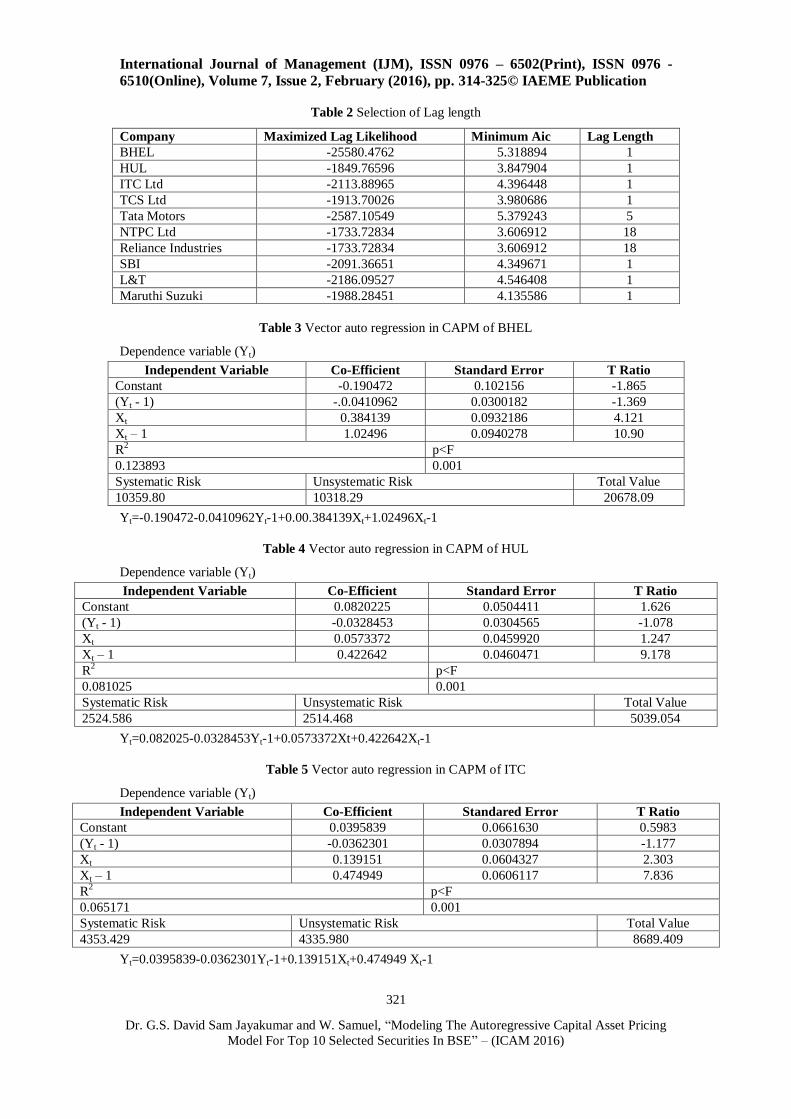
Table 2 Selection of Lag length

Company Maximized Lag Likelihood Minimum Aic Lag Length

BHEL -25580.4762 5.318894 1

HUL -1849.76596 3.847904 1

ITC Ltd -2113.88965 4.396448 1

TCS Ltd -1913.70026 3.980686 1

Tata Motors -2587.10549 5.379243 5

NTPC Ltd -1733.72834 3.606912 18

Reliance Industries -1733.72834 3.606912 18

SBI -2091.36651 4.349671 1

L&T -2186.09527 4.546408 1

Maruthi Suzuki -1988.28451 4.135586 1

Table 3 Vector auto regression in CAPM of BHEL

Dependence variable (Yt)

Independent Variable Co-Efficient Standard Error T Ratio

Constant -0.190472 0.102156 -1.865

(Yt - 1) -.0.0410962 0.0300182 -1.369

Xt 0.384139 0.0932186 4.121

Xt – 1 1.02496 0.0940278 10.90

R2 p<F

0.123893 0.001

Systematic Risk Unsystematic Risk Total Value

10359.80 10318.29 20678.09

Yt=-0.190472-0.0410962Yt-1+0.00.384139Xt+1.02496Xt-1

Table 4 Vector auto regression in CAPM of HUL


Independent Variable Co-Efficient Standard Error T Ratio

Constant 0.0820225 0.0504411 1.626

(Yt - 1) -0.0328453 0.0304565 -1.078

Xt 0.0573372 0.0459920 1.247

Xt – 1 0.422642 0.0460471 9.178

R2 p<F

0.081025 0.001


2524.586 2514.468 5039.054

Yt=0.082025-0.0328453Yt-1+0.0573372Xt+0.422642Xt-1

Table 5 Vector auto regression in CAPM of ITC


Independent Variable Co-Efficient Standared Error T Ratio

Constant 0.0395839 0.0661630 0.5983

(Yt - 1) -0.0362301 0.0307894 -1.177

Xt 0.139151 0.0604327 2.303

Xt – 1 0.474949 0.0606117 7.836

R2

p<F

0.065171 0.001


4353.429 4335.980 8689.409

Yt=0.0395839-0.0362301Yt-1+0.139151Xt+0.474949 Xt-1



322



Table 6 Vector auto regression in CAPM of TCS



Constant 0.119817 0.0532669 2.249

(Yt - 1) -0.147503 0.0294743 -5.004

Xt 0.228029 0.0485446 4.697

Xt – 1 0.597769 0.0491495 12.16

R2

p<F

0.158374 0.01


2811.523 2800.254 5611.777

Yt=0.119817 -0.147503Yt-1+0.228029Xt+0.597769Xt-1

Table 7 Vector auto regression in CAPM of Tata Motors

Dependence Variable (Yt)


Constant 0.00446181 0.103326 0.04318

(Yt- 1) 0.0928764 0.0318568 2.915

Xt 0.443119 0.0944525 4.691

Xt- 1 1.22838 0.0955808 12.85

R2

p<F

0.175099 0.001


10559.68 10390.40 20950.08

Yt=0.00446181-0.09287464Yt-1+0.443119Xt+1.22838Xt-1

Table 8 Vector auto regression in CAPM of L&T



Constant -0.0494641 0.0637248 -0.7762

(Yt - 1) -0.0666014 0.0273029 -2.439

Xt 0.165124 0.0582072 2.837

Xt – 1 -1.09155 0.0584666 18.67

R2

p<F

0.267515 0.001


4040.449 4024.257 8064.706

Yt=-0.0494641 -0.0666014Yt-1+0.165124Xt-1.09155Xt-1

Table 9 Vector auto regression in CAPM of Maruthi suzuki


Independent Variable Co-Efficient Standred Error T Ratio

Constant 0.0138608 0.0571264 0.2426

(Yt - 1) -0.0923460 0.0299030 -3.088

Xt 0.233942 0.0522380 4.478

Xt – 1 0.588735 0.0526759 11.18

R2 p<F

0.132061 0.001


3246.938 3233.923 6480.861

Yt=0.0138608 -0.0923460Yt-1+0.233942Xt+0.588735Xt-1



323



Table 10 Vector auto regression in CAPM of NTPC



Constant 0.102094 0.0434799 2.348

(Yt - 1) 0.187849 0.0324237 5.794

Xt 0.188936 0.0389880 4.846

Xt – 1 0.566252 0.0394435 14.36

R2 p<F

0.251645

0.001


1713.933 1619.479 3333.412

Yt=0.102094-0.187849Yt-1+0.188936Xt+0.566252Xt-1

Table 11 Vector auto regression in CAPM of Reliance Industries



Constant 0.0441659 0.0455255 0.9701

(Yt - 1) 0.223400 0.0324342 6.888

Xt 0.216965 0.0415716 5.219

Xt – 1 0.939941 0.0421485 22.30

R2 p<F

0.397976 0.001


1963.058 1854.875 3817.933

Yt=0.0441659 -0.223400Yt-1+0.216965Xt+0.939941Xt-1

Table 12 Vector auto regression in CAPM of SBI



Constant -0.0347306 0.0566486 -0.6131

(Yt - 1) -0.0916188 0.0268677 -3.410

Xt 0.278347 0.0517242 5.381

Xt – 1 1.03836 0.0524702 19.79

R2 p<F

0.303308 0.001


3193.191 3180.395 6373.586

Yt=-0.0347306 -0.0916188Yt-1+0.278347Xt+1.03836Xt-1

DISCUSSION

Table 1 exhibits the result of the test of normality security return list if top 10 companies in BSE. In

order to verify the test of normality in security return we employed four different statistical

test(Doornikhanseen Test,Shapiro Wilk W,Lillifors Test,Jarque-Bera Test) respectively the result of

the test source the security returns are not normally distributed one percent level of significant. The

source return of the company depreciated from normality and the followed non normal distribution.

Table2 visualizes the selection of maximum lag length will security return for each company the

maximum the likely loglikelihood returns and the maximum AIC where displayed the result of the

analyses source in order to perform for the analysis we have to proceed with maximum lag length of

each security returns Table 3exhibits the result of the extreme Dependent variable fitted as a capital

asset pricing model for the company returns of BHEL the result shows the beta value such as (Y t-1), is

negative and statistically significant 1% level. This shows if the BSE 30 indices will change then the



324



company returns will decrease. Moreover the R2 of 0.123893explain 12.38 % variation in the company

of BHEL. Finally, the systematic risk of company of BHEL is more and unsystematic risk is less. This

shows the market risk of the company of BHEL is less compared to the non-market risk. Table 4

exhibits the result of the extreme Dependent variable fitted as a capital asset pricing model for the

company returns of HUL the result shows the beta value such as (Yt-1) is negative and statistically

significant 1% level. This shows if the BSE 30 indices will change then the company returns will

decrease. Moreover the R2 of 0.081025explain 08.10 % variation in the company of HUL. Finally, the

systematic risk of company of HUL is more and unsystematic risk is less. This shows the market risk of

the company of HUL is less compared to the non-market risk.Table 5 exhibits the result of the extreme

Dependent variable fitted as a capital asset pricing model for the company returns of ITC the result

shows the beta value such as (Yt-1),Xt,(Xt-1) are positive and statistically significant 1% level. This

shows if the BSE 30 indices will change then the industry returns company will decrease. Moreover the

R2 of 0.123893explain 63.67 % variation in the company of BHEL. Finally, the systematic risk of

company of BHEL is more and unsystematic risk is less. This shows the market risk of the company of

BHEL is less compared to the non-market risk. Table 6 exhibits the result of the extreme Dependent

variable fitted as a capital asset pricing model for the company returns of BHELL the result shows the

beta value such as (Yt-1),Is negative and statistically significant 1% level.

This shows if the BSE 30 indices will change then the company returns will decrease. Moreover

the R2 of 0.158374 explain 15.83% variation in the company of ITC. Finally, the systematic risk of

company of ITC is more and unsystematic risk is less. This shows the market risk of the company of

ITC is less compared to the non-market risk. Table 7 exhibits the result of the extreme Dependent

variable fitted as a capital asset pricing model for the company returns of TATA MOTORS the result

shows the beta value such as (Yt-1),Xt,(Xt-1) are positive and statistically significant 1% level. This

shows if the BSE 30 indices will change then the company returns will decrease. Moreover the R2 of

0.175099explain 17.50% variation in the company of TATA MOTORS. Finally, the systematic risk of

company of TATA MOTORS is more and unsystematic risk is less. This shows the market risk of the

company of TATA MOTORS is less compared to the non-market risk. Table 8 exhibits the result of the

extreme Dependent variable fitted as a capital asset pricing model for the company returns of L&T the

result shows the beta value such as (Yt-1),(Xt-1) are negative and statistically significant 1% level. This

shows if the BSE 30 indices will change then the company returns will decrease. Moreover the R2 of

0.267515explain 26.75 % variation in the company of L&T. Finally, the systematic risk of company of

L&T is more and unsystematic risk is less. This shows the market risk of the company of L&T is less

compared to the non-market risk. Table 9 exhibits the result of the extreme Dependent variable fitted as

a capital asset pricing model for the company returns of MARUTHI SUZUKI the result shows the beta

value such as (Yt-1) Is negative and statistically significant 1% level.

This shows if the BSE 30 indices will change then the company returns will decrease. Moreover

the R2 of 0.132061explain 13.20% variation in the company of MARUTHI SUZUKI. Finally, the

systematic risk of company of MARUTHI SUZUKI is more and unsystematic risk is less. This shows

the market risk of the company of MARUTHI SUZUKI is less compared to the non-market

risk.Table10 exhibits the result of the extreme Dependent variable fitted as a capital asset pricing

model for the company returns of NTPC the result shows the beta value such as (Y t-1),Xt,(Xt-1) are

positive and statistically significant 1% level. This shows if the BSE 30 indices will change then the

company returns will decrease. Moreover the R2 of 0.251654 explain 25.16 % variation in the company

of NTPC. Finally, the systematic risk of company of NTPC is more and unsystematic risk is less. This

shows the market risk of the company of NTPC is less compared to the non-market risk. Table 11

exhibits the result of the extreme Dependent variable fitted as a capital asset pricing model for the

company returns of RELIANCE INDUSTRIES the result shows the beta value such as (Yt-1),Xt,(Xt-1)

are positive and statistically significant 1% level. This shows if the BSE 30 indices will change then the

company returns will decrease. Moreover the R2 of 0.397976 explain 39.79 % variation in the company

of Reliance Industries. Finally, the systematic risk of company of Reliance Industries is more and

unsystematic risk is less. This shows the market risk of the company of Reliance Industries is less

compared to the non-market risk.Table 12 exhibits the result of the extreme Dependent variable fitted

as a capital asset pricing model for the company returns of SBI the result shows the beta value such as

(Yt-1) is negative and statistically significant 1% level. This shows if the BSE 30 indices will change

then the company returns will decrease. Moreover the R2 of 0.303308explain 30.33% variation in the



325



company of SBI. Finally, the systematic risk of company of SBI is more and unsystematic risk is less.

This shows the market risk of the company of SBI is less compared to the non-market risk.

After analyzing the top 10 companies data,t he following recommendations were suggested to the

investors to invest and cautious to invest the market share respectively.

We find that the following company is less risk because the unsystematic risk or marketable risk is

less for securities. This shows the market risk of the following companies is less compared to the non-

marketable risk of the company. The companies are Reliance industries, BHEL, HUL, ITC, NTPC,

SBI, Maruthi Suzuki, L & T, TCS and Tata motors. So investors will made investment in this

companies it avoid risk of loss of securities.

CONCLUSION

The result on the study shows that the CAPM in Vector Auto Regression fitted on security returns and

company based on information criteria. In fitting the authors selected the best companies Reliance

industries, BHEL, HUL, ITC, NTPC, SBI, Maruthi Suzuki, L & T, TCS and Tata motors and

calculated the system risk and unsystematic risk of securities of company. So recommend to the

investor to invest the non-marketable risk of the companies which are suggested by our findings of

study.

REFERENCES

[1] Hamidreza Vakili Fard and Amin Babaei Falah (2015) A New Modified CAPM Model:

The Two Beta CAPM, Jurnal UMP Social Sciences and Technology Management, Vol. 3,

Issue 1, 2015

[2] , Stefan Daniel and Josef Glova (2015)Time-varying CAPM and its Applicability in Cost

of Equity Determination, Procedia Economics and Finance 32 ( 2015 ) 60 – 67

[3] Cenesizoglu, T., & Reeves, J. J. (2013) CAPM, Components of Beta and the Cross

Section of Expected Returns.

[4] Damodaran, A. (2012) An Intertemporal Capital Asset Pricing Model. Econometrica,

41(5), 867-888.

[5] Roodposhti, F. R., & Amirhosseini, Z. (2009) Common Risk Factors in the Returns on

Bonds and Stocks. Journal of Financial Economics, 33, 3- 56. 7.

[6] Gould, M. (2008) Investment Valuation: Tools and Techniques for Determining the Value

of Any Asset. Business & Economics.

[7] Estrada, J. (2007) The Arbitrage Theory of Capital Asset Pricing. Journal of Economic

Theory, 13, 341-360.

[8] Ryan, B. (2004) Mean-Semivariance Behavior: Downside Risk and Capital Asset Pricing.

International Review of Economics and Finance, 16, 169-185.

[9] Fama, E. F., & French, K. R. (1993) Investment Concepts. Journal of Research Starters

Business.

[10] Merton, R. C. (1973) Revised Capital Asset Pricing Model: an Improved Model for

Forecasting Risk and Return. Global Conf. On Business and Finance Proceeding.

Atlantic.

modeling the autoregressive capital asset pricing model for top 10 selected securities in bse

Engineering