modeling the bid/ask spread: measuring the inventory-holding

Journal of Financial Economics 72 (2004) 97–141

Modeling the bid/ask spread: measuring theinventory-holding premium$

Nicolas P.B. Bollena, Tom Smithb, Robert E. Whaleyc,*aOwen Graduate School of Management, Vanderbilt University, Nashville, TN 37203, USA

bAustralian National University, Canberra, ACT 0200, AustraliacFuqua School of Business, Duke University, Durham, NC 27708, USA

Received 9 July 2002; accepted 10 December 2002

Abstract

The need to understand and measure the determinants of market maker bid/ask spreads is

crucial in evaluating the merits of competing market structures and the fairness of market

maker rents. This study develops a simple, parsimonious model for the market maker’s spread

that accounts for the effects of price discreteness induced by minimum tick size, order-

processing costs, inventory-holding costs, adverse selection, and competition. The inventory-

holding and adverse selection cost components of spread are modeled as an option with a

stochastic time to expiration. This inventory-holding premium embedded in the spread

represents compensation for the price risk borne by the market maker while the security is held

in inventory. The premium is partitioned in such a way that the inventory-holding and adverse

selection cost components, as well as the probability of an informed trade, are identified. The

model is tested empirically using Nasdaq stocks in three distinct minimum tick size regimes

and is shown to perform well both in an absolute sense and relative to competing

specifications.

r 2003 Elsevier B.V. All rights reserved.

ARTICLE IN PRESS

$Comments and suggestions by Tim Brailsford, F. Douglas Foster, Stephen Gray, Chris Kirby, Craig

Lewis, Stewart Mayhew, Hans Stoll, George Wang, and the seminar participants at the University of

Otago, Dunedin, New Zealand, the Australian National University, Canberra, Australia, the Accounting

and Finance Research Camp, Australian Graduate School of Management, University of New South

Wales, Sydney, Australia, the Melbourne Business School, Melbourne, Australia, Commodity Futures

Trading Commission, Washington, DC, Queensland Business School, University of Queensland, Brisbane,

Australia, and Vanderbilt University, Nashville, Tennessee are gratefully acknowledged. This research is

supported by the Australian Research Council SPIRT Grant C00001858. The comments and suggestions

of an anonymous referee are gratefully acknowledged.

*Corresponding author.

E-mail address: [email protected] (R.E. Whaley).

0304-405X/$ - see front matter r 2003 Elsevier B.V. All rights reserved.

doi:10.1016/S0304-405X(03)00169-7

JEL classification: D23; G12; G13; G14; L22

Keywords: Bid/ask spread; Inventory-holding premium; Expected insurance cost; Semi-variance;

Stochastic time to expiration

1. Introduction

Understanding the determinants of the market maker’s bid/ask spread isimportant for a variety of reasons. From an exchange’s standpoint, it providesguidance on market design. Should the exchange assign a single specialist to beresponsible for making a market, or should it encourage competition among anumber of willing market makers? It also provides guidance on setting an optimalminimum tick size. In a competitive market, the tick size can provide market makerswith a means of recovering their fixed costs of operation. From a regulator’sstandpoint, the bid/ask spread provides a means of identifying the fairness of therents being extracted by market makers. Are market makers extracting abnormallyhigh rents for their services, or are the rents fair considering the market maker’s costsof operation?Prior research has made substantial progress toward understanding the

determinants of the bid/ask spread. Initial work, including studies by Demsetz(1968), Tinic (1972), Tinic and West (1972, 1974), Benston and Hagerman (1974),and Branch and Freed (1977), focuses on empirically determining which variablescan capture cross-sectional variation in spreads. Stoll (1978b) develops a theoreticalmodel for spreads in order to impose structure on the problem, and provides a usefulcategorization of the costs of supplying liquidity. Harris (1994) shows that amarket’s tick size can affect the estimated relation between the bid/ask spread and itsdeterminants. While these studies all have made significant contributions to theunderstanding of the bid/ask spread, an important unresolved issue is the functionalform of the relation between spread and its explanatory variables.The purpose of this paper is to develop and test a new model of the market

maker’s bid/ask spread. The model is simple, parsimonious, and well grounded froma theoretical perspective. It incorporates the effects of price discreteness induced bythe minimum tick size, order-processing costs, inventory-holding costs, adverseselection costs, and competition. The inventory-holding and adverse selection costcomponents of spread are modeled as an option with a stochastic time to expiration.This inventory-holding premium embedded in the spread represents compensationfor price risk borne by the market maker while the security is held in inventory,independent of whether the trade was with an informed or an uninformed trader.Moreover, the premium can be partitioned in such a way that the inventory-holdingand adverse selection cost components can be identified and estimated. Indeed, themodel is rich enough to identify the probability of an informed trade. The model istested using three separate months of Nasdaq common stock data corresponding tothree different tick size regimes (eighths in March 1996, sixteenths in April 1998, anddecimal pricing in December 2001) and is strongly supported empirically.

ARTICLE IN PRESSN.P.B. Bollen et al. / Journal of Financial Economics 72 (2004) 97–14198

The paper proceeds as follows. Section 2 contains a discussion of the theoreticaland empirical literature on market maker spreads. We provide a generalcategorization of the costs associated with market making and a brief review ofpast work. Section 3 contains the formal development of our theoretical model andcontrasts its structure with the models used in earlier work. Section 4 contains anempirical assessment of the model and examines the importance of modelspecification in providing meaningful inference regarding the determinants ofspread. We also highlight problems of variable selection and estimation that candistort inference, estimate the probability of informed trades, and provide abreakdown of the cost components of the spread. Section 5 contains a briefsummary.

2. Market making costs

This section describes the cost components of the market maker’s bid/ask spreadin a cross-sectional framework and examines how past researchers have measuredthese costs.1 The discussion of the cost components is organized in the manner ofStoll (1978b), who posits that market maker costs fall into three categories: order-processing costs, inventory-holding costs, and adverse selection costs.2 Discussionsof the effects of competition and the structural form of the model follow. The proxyvariables used in past studies are summarized in Table 1.

2.1. Order processing costs

Order-processing costs are those directly associated with providing the marketmaking service and include items such as the exchange seat, floor space rent,computer costs, informational service costs, labor costs, and the opportunity cost ofthe market maker’s time. Because these costs are largely fixed, at least in the shortrun, their contribution to the size of the bid/ask spread should fall with tradingvolume; that is, the higher the trading volume, the lower the bid/ask spread. To somedegree, however, this relation may be weakened by the fact that market makers oftenmake markets in more than one security. In such cases, fixed order-processing costscan be amortized over total trading volume across securities. In addition, in a highly

ARTICLE IN PRESS

1The discussion in this section focuses on the determinants of spread literature for the stock market and

how it developed in the years following the pioneering work of Demsetz (1968). It is not meant to provide

a comprehensive review of cross-sectional investigations of spreads in the stock market that address a

variety of interesting policy issues including market structure (e.g., Bessembinder and Kaufman, 1997;

Ellis et al., 2002), tick size (e.g., Bacidore, 1997; Bollen and Whaley, 1998; Goldstein and Kavajecz, 2000;

Jones and Lipson, 2001; Bessembinder, 2003), and order-processing rules (e.g., Bessembinder, 1999;

Weston, 2000). Nor is it intended to diminish the importance of investigations of the determinants of the

bid/ask spread in nonstock markets (e.g., Neal, 1987, on stock option markets; George and Longstaff,

1993, on index options; Smith and Whaley, 1994, on index futures).2For a comprehensive review of the market microstructure literature, see Stoll (2003).

N.P.B. Bollen et al. / Journal of Financial Economics 72 (2004) 97–141 99

ARTIC

LEIN

PRES

S

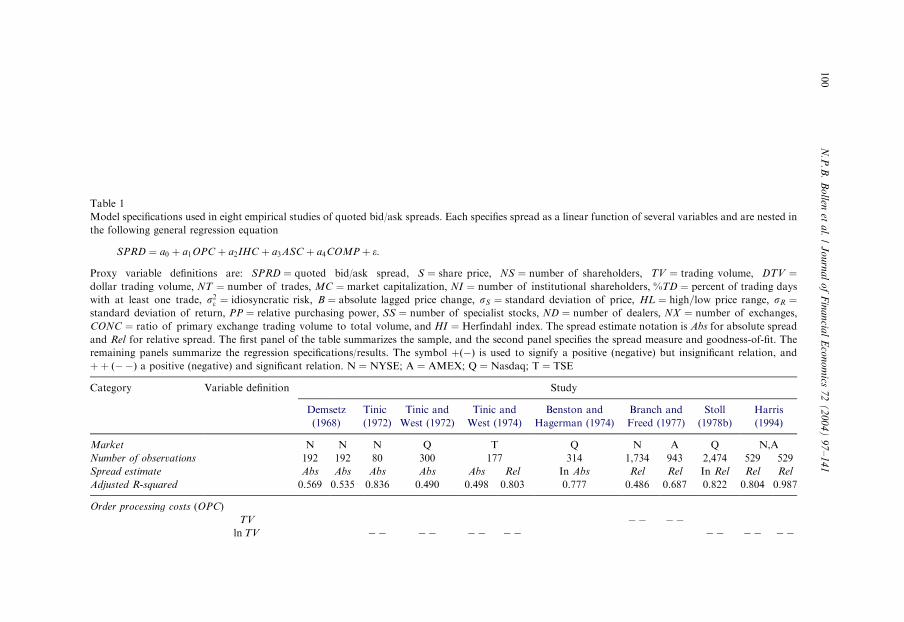
Table 1

Model specifications used in eight empirical studies of quoted bid/ask spreads. Each specifies spread as a linear function of several variables and are nested in

the following general regression equation

SPRD ¼ a0 þ a1OPC þ a2IHC þ a3ASC þ a4COMP þ e:

Proxy variable definitions are: SPRD ¼ quoted bid/ask spread, S ¼ share price; NS ¼ number of shareholders; TV ¼ trading volume; DTV ¼dollar trading volume; NT ¼ number of trades; MC ¼ market capitalization; NI ¼ number of institutional shareholders; %TD ¼ percent of trading days

with at least one trade, s2e ¼ idiosyncratic risk; B ¼ absolute lagged price change; sS ¼ standard deviation of price; HL ¼ high=low price range; sR ¼standard deviation of return; PP ¼ relative purchasing power; SS ¼ number of specialist stocks; ND ¼ number of dealers; NX ¼ number of exchanges;CONC ¼ ratio of primary exchange trading volume to total volume; and HI ¼ Herfindahl index: The spread estimate notation is Abs for absolute spread

and Rel for relative spread. The first panel of the table summarizes the sample, and the second panel specifies the spread measure and goodness-of-fit. The

remaining panels summarize the regression specifications/results. The symbol þð�Þ is used to signify a positive (negative) but insignificant relation, and

þþ ð��Þ a positive (negative) and significant relation. N ¼ NYSE; A ¼ AMEX; Q ¼ Nasdaq; T ¼ TSE

Category Variable definition Study

Demsetz

(1968)

Tinic

(1972)

Tinic and

West (1972)

Tinic and

West (1974)

Benston and

Hagerman (1974)

Branch and

Freed (1977)

Stoll

(1978b)

Harris

(1994)

Market N N N Q T Q N A Q N,A

Number of observations 192 192 80 300 177 314 1,734 943 2,474 529 529

Spread estimate Abs Abs Abs Abs Abs Rel In Abs Rel Rel In Rel Rel Rel

Adjusted R-squared 0.569 0.535 0.836 0.490 0.498 0.803 0.777 0.486 0.687 0.822 0.804 0.987

Order processing costs (OPC)

TV �� ln TV ��

N.P

.B.

Bo

llenet

al.

/J

ou

rna

lo

fF

ina

ncia

lE

con

om

ics7

2(

20

04

)9

7–

14

1100

ARTIC

LEIN

PRES

SlnDTV

1=NT1=2 þþ þþ

Inventory holding costs (IHC)

ln NS �� ln NT ��

NI ��%TD �� ln S þþ ��1=S þþ þþ þþS þþ þþ þþ þþ þþ þþ

ln s2e þþB=S þþ þþsS þ

HL=S þ þþ þþsR þþ þþln s2R þþPP �

Adverse selection costs (ASC)

SS þþ þþ þln DTV=MC þþ

ln MC þþ þ

Competition (COMP)

ln ND �� NX � � � � ��

lnCONC þþ �� HI þþND ��

N.P

.B.

Bo

llenet

al.

/J

ou

rna

lo

fF

ina

ncia

lE

con

om

ics7

2(

20

04

)9

7–

14

1101

competitive market, bid/ask spreads should equal the expected marginal cost ofsupplying liquidity, in which case order-processing costs may be irrelevant.

2.2. Inventory-holding costs

Inventory-holding costs are the costs that a market maker incurs while carryingpositions acquired in supplying investors with immediacy of exchange (liquidity).Here there are two obvious considerations: the opportunity cost of funds tied up incarrying the market maker’s inventory and the risk that the inventory value willchange adversely as a result of security price movements. With respect to theopportunity cost of funds, Demsetz (1968, p. 45) argues that price per share is areasonable proxy.

Spread per share will tend to increase in proportion to an increase in the price pershare so as to equalize the cost of transacting per dollar exchanged. Otherwise,those who submit limit orders will find it profitable to narrow spreads on thosesecurities for which spread per dollar exchanged is larger.

His argument is that relative spread (bid/ask spread divided by bid/ask midpoint)should be equal across stocks, holding other factors constant, or the higher the shareprice, the higher the spread. Market makers try to reduce or close out positionsbefore the close of trading each day, however. If positions are opened and closed inthe same day, the marginal cost of financing is zero. Moreover, even if inventory iscarried overnight, it is not clear whether it represents a cost or a benefit. If, duringthe day, most customer orders are buys, the market maker may be short inventory,in which case he will earn (not pay) interest overnight.Price-change volatility appears to have an unambiguous effect on the bid/ask

spread. Market makers often carry inventory in the course of supplying liquidity,and hence bear risk. The size of the spread therefore must include compensation forbearing the risk. Demsetz includes trade frequency and the number of shareholdersas proxies for this component of inventory-holding costs. Both variables, he argues,are direct proxies for the transaction rate. The higher the transaction rate, the lowerthe cost of waiting (price-change volatility equals the price-change volatility ratedivided by trading frequency), and hence the lower the bid/ask spread. Tinic (1972)chooses to include a direct measure of volatility; that is, the standard deviation ofprice as a measure of inventory price risk. Tinic and West (1972) measure price riskas the ratio of the difference between high and low prices to the average share price,Benston and Hagerman (1974) use the stock’s idiosyncratic risk, Stoll (1978b) usesthe logarithm of the variance of stock returns, and Harris (1994) uses the standarddeviation of returns.3

ARTICLE IN PRESS

3Benston and Hagerman (1974) argue that the market maker needs to be rewarded for price risk only to

the extent that he is not well diversified or is exposed to traders with superior information (i.e., adverse

selection costs). The concept of adverse selection had been introduced a few years earlier by Bagehot

(1971).

N.P.B. Bollen et al. / Journal of Financial Economics 72 (2004) 97–141102

2.3. Adverse selection costs

Adverse selection costs arise from the fact that market makers, in supplyingimmediacy, may trade with individuals who are better informed about the expectedprice movement of the underlying security. For an individual stock, it is easy toimagine that certain individuals possess insider information (e.g., advance news ofearnings, restructurings, and management changes). While the intuition underlyingwhy adverse selection may be an important determinant of spread is clear, theselection of an accurate measure of adverse selection costs is not. Branch and Freed(1977), for example, use the number of securities in which a dealer makes a market toproxy for adverse selection—the larger the number of securities managed, the lessinformed the dealer is, on average, about a particular stock. Stoll (1978a) uses ameasure of turnover (dollar trading volume divided by market capitalization)—thehigher the turnover, the greater the adverse selection. Glosten and Harris (1988) usethe concentration of ownership by insiders—the higher the concentration, thegreater the possibility of adverse selection. Harris (1994) uses the market value ofshares outstanding—the larger the firm, the more well known and hence the lowerthe possibility of adverse selection. Easley et al. (1996) use the volume of trading—the higher the trading volume, the greater the activity of uninformed traders relativeto informed traders and the lower the adverse selection cost.

2.4. Competition

The level of the market maker’s bid/spread is also likely to be affected by the levelof competition, particularly in an environment in which barriers to entry in themarket for markets are being slowly eliminated. As competition increases, the bid/ask spread approaches the expected marginal cost of supplying liquidity; that is, thesum of inventory-holding costs and adverse selection costs. The larger the number ofmarket makers, the greater the competition and the lower the bid/ask spread.Anshuman and Kalay (1998) show that, if the start-up costs of creating a competingexchange are significant, the tick size (the security’s minimum price increment) canbe set high enough that market makers can recoup their fixed costs as well as earn aneconomic profit.Of the wide variety of proxies that have been used to measure competition, the

most precise is the Herfindahl index of concentration introduced into the marketmicrostructure literature by Tinic (1972). The index is

HI ¼XNM

j¼1

Vj

TV

� �2

; ð1Þ

where Vj is the number of shares traded by market maker j;NM is the number ofmarket makers, and TV ¼

PNMj¼1 Vj is the total number of shares traded by all

market makers. The index has a range from 1=NM to 1, where 1=NM is the lowestconcentration (perfect competition) and 1 is the highest (monopoly).

ARTICLE IN PRESSN.P.B. Bollen et al. / Journal of Financial Economics 72 (2004) 97–141 103

2.5. Structural form

The cross-sectional tests summarized in Table 1 impose a particular functionalform on the relation,

SPRDi ¼ f ðOPCi; IHCi;ASCi;COMPÞ; ð2Þ

where SPRDi is the difference between a security’s bid and ask quotes (bid/askspread), OPCi is order-processing costs, IHCi is inventory-holding costs, ASCi isadverse selection costs, and COMPi is the degree of competition.4 The earlieststudies used absolute spread as the dependent variable and allowed the independentvariables to enter the regression linearly. Tinic and West (1974), for example,estimate a model of absolute spread with price per share, log of trading volume, pricevolatility (as measured by the high-low price range divided by price), tradingcontinuity (as measured by the number of days the stock is traded during the sampleperiod divided by the total number of days in the sample period), and the number ofmarkets in which the security is traded, and they find that the adjusted R-squared inthe regression is 0.499. They also estimate the model when relative spread is used asthe dependent variable, dropping price per share as an explanatory variable, and findthat the adjusted R-squared is 0.804. The most powerful explanatory variable turnsout to be price volatility, whose coefficient is positive and highly significant.Using relative spread as the dependent variable is problematic for at least two

reasons. First, if the regression equation for the absolute spread is correctly specifiedbased on theoretical arguments, the regression equation for the relative spread is not.For the relative spread regression to be correctly specified, all of the explanatoryvariables must be deflated by share price. This means running the regression linethrough the origin. Second, given the high level of the adjusted R-squared, therelative spread regression gives the misleading impression of being a powerfulexplanatory model of bid/ask spread.5 To see this, assume that all stock spreads inthe sample are equal to one-eighth. In such an environment, the absolute spreadregression model would have no explanatory power. All of the coefficient valueswould equal zero, except the intercept term whose value would be one-eighth. Now,consider the relative spread regression. Given that the absolute spread is assumed to

ARTICLE IN PRESS

4Spread determinant studies now tend to analyze the time-series properties of observed transaction price

changes. Roll (1984) pioneers this type of analysis by introducing a serial covariance estimator of the bid/

ask spread that relies only on a sequence of transaction prices and provides an estimate only of order

processing costs. Stoll (1989) develops a more complex model that allows simultaneous estimation of order

processing costs, inventory-holding costs, and adverse selection costs. George et al. (1991) correct for bias

in estimation of the spread and its components, and they conclude that adverse selection costs are much

smaller than previously reported. Huang and Stoll (1997) provide a general framework that nests a large

number of these statistical models and, consistent with George et al. (1991), report empirical evidence that

the order-processing cost is the dominant determinant of spread. Other studies have used this type of

component analysis to investigate the impact of market structure, news announcements, trade size, and

other features of a market on the different components of bid/ask spread. See, for example, Affleck-Graves

et al. (1994), Lin et al. (1995), Krinsky and Lee (1996), and Keim and Madhavan (1997).5For a lucid discussion of the pitfalls of using ratio variables in a regression framework, see Kronmal

(1993).


be constant, the variation in the dependent variable is driven only by variation in theinverse of share price. Not surprisingly, explanatory variables such as price volatilityare significant in a statistical sense, not because the regression is saying anythingmeaningful about spreads, but because the price volatility variable has share price inits denominator. As the variation in the share price range across stocks becomessmall, the goodness-of-fit of the relative spread regression will become perfect.The structural form of the model is also a concern. The models discussed thus far

were developed through economic reasoning instead of formal mathematicalmodeling. Given their ad hoc nature, they are open to criticisms regarding modelspecification and variable selection. In an attempt to analyze the supply of dealerservices (liquidity) more rigorously, Stoll (1978b) develops an explicit theoreticalmodel that shows that the relative bid/ask spread of a security equals the sum ofinventory-holding costs, adverse selection costs, and order-processing costs, wheneach cost component has a precise definition. The inventory-holding cost expressionincludes a term that equals the product of return volatility and the expected time themarket maker expects the position to be open, a distinction that had otherwise goneunnoticed in the literature.

3. Model specification

We now develop a formal model of the market maker’s bid/ask spread.

3.1. Modeling expected inventory-holding costs

In principle, the market maker’s spread needs to include a premium to coverexpected inventory-holding costs, independent of whether the trade is initiated by aninformed or an uninformed customer. For convenience, assume initially that thelength of time a stock will be in inventory is known and short (e.g., minutes). Forsuch a short holding period, it is reasonable to assume that the risk-free rate and theexpected change in the true price of the stock are equal to zero.6 Suppose the dealertakes a long position in a share of stock as a result of accommodating a customer sellorder. To manage the inventory-holding risk of the position, he could potentiallyshort a single stock futures, assuming such a contract traded, until the long stockposition is unwound with a customer buy order. If the market maker’s objectivefunction is to minimize the variance of the value changes of his hedged portfolio—i.e., operates within a Markowitz (1952) mean–variance framework—and the stockfutures market is transaction cost-free, the optimal number of futures contracts forthe market maker to sell per share held is determined by

MinE½ðDS þ nFDF Þ2�; ð3Þ

where DS is the change in stock price, DF is the change in futures price, and nF is thehedge ratio. Setting the first-order condition equal to zero and rearranging shows

ARTICLE IN PRESS

6 It is also reasonable to ignore cash dividends, as the holding period is intraday while dividends are paid

overnight.


that the optimal hedge ratio is nF ¼ �CovðDS;DF Þ=VarðDF Þ:7 Assuming a zerointerest rate and dividend yield rate on the stock and perfect correlation between thestock price changes and the futures price changes, the optimal hedge is to sell onefutures contract for each share of stock. Under these ideal market conditions, themarket maker is able to eliminate the risk of adverse price changes.Stock futures do not provide a viable hedging vehicle for stock market makers,

however. The main reason is trading costs. For the few stocks whose futures nowtrade, trading costs in the futures markets are higher and liquidity is lower than inthe stock market, and this situation is unlikely to change.8 Hedging will not takeplace in an environment in which the market maker has round-turn trading coststhat exceed the revenue he can earn in the stock market.In the absence of a viable hedging instrument, the market maker faces inventory-

holding price risk for which he will demand compensation. We assume that themarket maker wants to set his inventory-holding premium ðIHPÞ such that heminimizes the risk of losing money should the market move against him; that is,

MinE½ðDS þ IHP j DSo0Þ2�: ð4Þ

The risk measure Eq. (4) is called the lower semi-variance. Setting the first-ordercondition to zero shows that the minimum inventory-holding premium that themarket maker is willing to charge is,

IHP ¼ �EðDS j DSo0ÞPrðDSo0Þ: ð5Þ

According to Eq. (5), the minimum IHP equals the expected loss on the tradeconditional on an adverse stock price movement times the probability of an adversestock price movement.The idea of applying lower semi-variance as a risk measure is not new. Markowitz

(1959) was the first to suggest using semi-variance instead of variance as the riskmeasure in the investor’s portfolio allocation decision, noting that variance is tooconservative because it regards all extreme returns, positive or negative, asundesirable. Ultimately he chose to use variance because of its familiarity and easeof computation.9 The Markowitz (1952) mean–variance framework went on to serveas the foundation of the portfolio separation work of Tobin (1958) and equilibriumcapital asset pricing model (CAPM) of Sharpe (1964) and Lintner (1965). Bawa andLindenberg (1977) develop a capital market equilibrium model in which expectedutility maximizing individuals make their portfolio allocation decisions based on themean and second-order lower partial moment of return distributions. They show

ARTICLE IN PRESS

7This result was first shown in Ederington (1979).8Until recently, stock futures were not traded in the United States. Outside the United States, the

trading activity in stock futures markets (e.g., the Sydney Futures Exchange in Australia and the Hong

Kong Futures Exchange in Hong Kong) has been dismal. On November 8, 2002, stock futures began

trading on the OneChicago Exchange in Chicago and the Nasdaq Liffe Markets in New York. For the

stock futures currently listed, average daily trading volume is less than half of 1% of the average daily

volume in the stock market.9Mao (1970) compares the use of expected return–variance and expected return–semi-variance models

in the context of capital budgeting. Markowitz (1991) continues to argue the superiority of semi-variance

over variance as a risk measure.


that, if the lower partial moment is calculated using the risk-free rate as the targetreturn, the familiar separation and equilibrium properties of the CAPM hold. Morerecently, the expected loss conditional on an adverse price movement has appearedin the risk management literature, where it has been dubbed expected shortfall andconditional value-at-risk. The virtues of this measure are described in Artzner et al.(1999) and Szeg .o (2002).The value of the inventory-holding premium given by the expression on the right

hand-side of Eq. (5) equals the value of an at-the-money option with expiration givenby the time that the stock is held in inventory. Suppose a market maker who has noinventory accommodates a customer order by buying at the bid. He needs protectionagainst the price falling below his purchase price before he can unwind his position.Conversely, if the market maker has no inventory and accommodates a customerorder to buy by selling at the ask, he needs protection against the price rising abovehis sales price. In the first case, the market maker needs to buy an at-the-money putwritten on the stock, and, in the second, he needs to buy an at-the-money call. Likeindividual stock futures, individual stock options do not represent viable hedgingvehicles for market makers in stocks. For one thing, the bid/ask spreads in the stockoption market are at least as high as in the stock market. For another, the times toexpiration and the exercise prices of the available option series are unlikely to matchhedging needs. Nonetheless, the Black and Scholes (1973) and Merton (1973)(hereafter, BSM) option valuation framework provides a convenient means formeasuring the IHP: Suppose the market maker needs to buy a call. Using the BSMoption valuation formula, the expected inventory-holding premium may be written

IHP ¼ SNlnðS=X Þ

sffiffit

p þ 0:5sffiffit

p !� XN

lnðS=X Þ

sffiffit

p � 0:5sffiffit

p !; ð6Þ

where S is the true stock price at the time at which the market maker opens hisposition, X is the exercise price of the option, s is the standard deviation of securityreturn, t is the time until the offsetting order, and NðÞ is the cumulative unit normaldensity function.10 The expected loss described by Eq. (5) is an at-the-money option,so the valuation formula Eq. (6) simplifies to

IHP ¼ S½2Nð0:5sffiffit

pÞ � 1�: ð7Þ

3.2. Stochastic time to offsetting trade

The difficulty in valuing the expected inventory-holding premium using Eq. (7) isthat the market maker, at the time of trade, does not know when an offsettingtransaction will occur. The appropriate inventory-holding premium is thereforestochastic:gIHPIHP ¼ S½2Nð0:5sfffiffitpffiffitp Þ � 1�: ð8Þ

ARTICLE IN PRESS

10The inventory-holding premium may also be valued using the put valuation formula, which leads to

identical results.


To set the spread at a level that provides sufficient revenue to generate anappropriate expected profit, the market maker must evaluate the expected inventory-holding premium. Defining pðtÞ as the probability distribution function of anoffsetting trade arriving at time t; the expected inventory-holding premium can beexpressed as

EðgIHPIHPÞ ¼Z

N

0

S½2Nð0:5sffiffit

pÞ � 1� pðtÞ dt; ð9Þ

which is tantamount to valuing a European-style option with a stochastic time toexpiration.11

One way to implement Eq. (9) as a means of estimating the expected IHP is toselect a reasonable and tractable distribution for the arrival rate of offsetting trades.Garman (1976), for example, models the arrival of traders as a Poisson distribution.This provides the necessary tractability. Under Poisson arrivals, the probabilitydistribution function of an order arriving at time t is

pðtÞ ¼ le�lt; ð10Þ

where l is the mean arrival rate. The expected IHP becomes

EðgIHPIHPÞ ¼Z

N

0

S½2Nð0:5sffiffit

pÞ � 1�le�lt dt: ð11Þ

For the problem at hand, however, we can avoid specifying a particular distributionof the arrival of an offsetting order because the expected hedging cost isapproximately linear in

ffiffit

p: A proof is contained in Appendix A. Thus, the market

maker’s expected IHP can be computed as

EðgIHPIHPÞ ¼ S½2Nð0:5sEðfffiffitpffiffitp ÞÞ � 1�; ð12Þ

where Eðfffiffitpffiffitp Þ is the expected value of the square root of the time between offsettingtrades. This expectation is easily estimated using transaction data and is the onlyaspect of the distribution of arrivals that is necessary to approximate expected IHP:Fig. 1 shows the expected IHP as a function of the volatility rate and the timebetween trades. For plausible parameter ranges, the expected IHP can be as high as16 cents.

3.2.1. Option collar—sharing the upside

The expected inventory-holding premium, modeled as an at-the-money call, maybe overstated. If the market maker has no inventory and accommodates a customerbuy order by selling at the ask, the expected inventory-holding premium is the valueof an at-the-money call. After the call is in place, however, the market maker is notonly protected against unexpected increases in the stock price, but also enjoys gainsif the stock price falls. If the market is highly competitive, part of this speculativeprivilege will be bid away, and the expected inventory-holding premium will equal the

ARTICLE IN PRESS

11The problem is analogous to that addressed by Merton (1976). Chang et al. (1998) use a similar

framework for valuing futures options in information time instead of calendar time.


value of the at-the-money call less the value of an out-of-the-money put (an optioncollar). If the stock price rises, the market maker is protected. If the stock price falls,the market maker’s gain is limited to the difference in exercise prices. Naturally, ifdealers in the stock market were perfectly competitive and had access to complete andfrictionless derivatives markets, the exercise prices of the call and the put would be thesame and the inventory-holding premium (the collar value) would be equal to zero.Individual stock futures and options markets are neither complete nor frictionless,however. The difference between the exercise prices of the call and the put will remainas long as there is no cost-effective means of hedging stock price risk.In practice, however, little is lost by using only the at-the-money call as a measure

of the expected IHP: A market maker will choose to minimize the inventory-holdingpremium (i.e., sell the out-of-the-money put) only in a highly competitive market. Insuch a market, the likelihood of the put going in-the-money is small. Fig. 2 shows theexpected IHP modeled as an option collar as a function of the volatility rate and thetime between trades, and Fig. 3 shows the difference between the expected inventory-holding premium modeled as an at-the-money call (Fig. 1) and the expected hedgingcosts modeled as an option collar (Fig. 2). The stock price is set equal to $27:50; thedifference between exercise prices is set equal to $0:25; the average time between

ARTICLE IN PRESS

0

5

10

15

20

0%

50%

100%

0

0.02

0.04

0.06

0.08

0.1

0.12

0.14

0.16

0.18

0.2

Inve

ntor

y ho

ldin

g pr

emiu

m

Minutes between trades

Volatility

Fig. 1. Relation between expected inventory-holding premium modeled as an at-the-money call and the

volatility rate and trading frequency of the stock. Stock price is set equal to $27.50. Volatility rate varies

between 0% and 100%, and number of minutes between trades varies from 0 to 20.


trades ranges from 0 to 20 min; and the volatility rate ranges from 0% to 100%. Asthe figures show, practically no difference exists between the values of the twomethods of modeling expected costs. Slight differences appear at the highest levels ofvolatility and the longest times between trades. These parameter settings are atypicalfor the Nasdaq stocks in our sample, however. The interquartile range for thevolatility rate in the April 1998 sample, for example, is 38.3–62.3%, and theinterquartile range for the number of minutes between trades is 1.32–6:28 min: Inthese ranges, Fig. 3 shows that the value of the out-of-the-money put is negligible. Inother words, using the more parsimonious at-the-money call value as an instrumentfor the expected inventory-holding premium appears well-justified.This is not the first application of option pricing in the study of market maker

spreads.12 Copeland and Galai (1983) model the adverse selection component of thebid/ask spread as a straddle in which the market maker provides informed traders

ARTICLE IN PRESS

0

5

10

15

20

0%50%

100%

0

0.02

0.04

0.06

0.08

0.1

0.12

0.14

0.16

0.18

0.2

Inve

ntor

y ho

ldin

g pr

emiu

m


Volatility

Fig. 2. Relation between expected inventory-holding premium modeled as an option collar (at-the-money

call less out-of-the-money put) and the volatility rate and trading frequency of the stock. Stock price is set

equal to $27.50. Volatility rate varies between 0% and 100%, and number of minutes between trades

varies from 0 to 20.

12 In a related context, Day and Lewis (2003) use the value of a barrier option to examine the adequacy

of initial margins in the crude oil futures market.


with a free-trading option to buy at the ask price or to sell at the bid. The option’stime to expiration is the interval over which the market maker quotes are held firm.We use an option-based inventory-holding premium to cover both the inventory-holding and adverse selection cost components of the spread. That is, the marketmaker buys a single at-the-money option as insurance against adverse pricemovements while the security is held in inventory. The option’s life begins once aquote is hit and remains open the expected length of time between offsetting trades.The empirical distinction between the approaches is highlighted in Section 4.

3.3. Informed versus uninformed traders

A market maker will demand different expected inventory-holding premia fortrades with informed and uninformed traders. Assume that the market makercurrently has no inventory, and a trader steps forward and buys at the marketmaker’s posted ask price, Sask: The market maker, now short a share of stock, isconcerned about his expected loss should the share price increase. If the trader isuninformed ðUÞ; the expected inventory-holding premium, IHPU ; equals the value ofa slightly out-of-the-money call option with an exercise price equal to Sask:

ARTICLE IN PRESS

0

5

10

15

20

0%50%

100%

0

0.02

0.04

0.06

0.08

0.1

0.12

0.14

0.16

0.18

0.2

Inve

ntor

y ho

ldin

g pr

emiu

m


Volatility

Fig. 3. Difference between expected inventory-holding premium modeled as an at-the-money call and

expected inventory-holding premium modeled as an option collar as a function of the volatility rate

and trading frequency of the stock. Stock price is set equal to $27.50. Volatility rate varies between 0% and

100%, and number of minutes between trades varies from 0 to 20.


Presumably the true price of the underlying stock is somewhere between the bid andask price quotes. If the trader is informed ðIÞ; the true price of the stock restssomewhere above the ask price, in which case the expected inventory-holdingpremium, IHPI ; equals the value of a slightly in-the-money call. In both cases, thevaluation of the IHP is

IHPi ¼ SiNlnðSi=X Þ

sffiffit

p þ 0:5sffiffit

p !� XN

lnðSi=X Þ

sffiffit

p � 0:5sffiffit

p !; ð13Þ

where i ¼ U ; I depending upon whether the trade was with an uninformed or aninformed trader.13

From the market maker’s perspective, the expected inventory-holding premium,IHP; equals the sum of the inventory-holding cost and adverse selection costcomponents of the spread. It can be expressed as a weighted sum of the two premia;that is,

IHP ¼ ð1� pI ÞIHPU þ pI IHPI ; ð14Þ

where pI ð1� pI Þ is the probability of an informed (uninformed) trade. Under thisformulation, the expected IHP does not go to zero as the time between offsettingtrades goes to zero. As t-0; the inventory-holding premium of an uninformed tradeIHPU approaches zero, but the inventory-holding premium of the informed tradeIHPI approaches the dollar amount the option is in the money (i.e., the differencebetween the true price and the ask price in the case of a buy, and the differencebetween the bid price and the true price in the case of a sell). Thus, when the timebetween offsetting trades is zero, the market maker demands compensation for theexpected loss to informed traders: IHP ¼ pI IHPI :Another way of interpreting the inventory-holding premium is to rewrite Eq. (14)

as

IHP ¼ IHPU þ pI ðIHPI � IHPU Þ: ð15Þ

What Eq. (15) says is that an expected inventory-holding premium of IHPU existsfor all trades, uninformed and informed alike, as a result of the price risk associatedwith having the security in inventory. For informed trades, however, an incrementalexpected cost is associated with adverse selection that equals the probability of aninformed trade times the incremental cost, pI ðIHPI � IHPU Þ: The structure ofEq. (15) also provides a means of estimating the probability of informed trades inone of the regression specifications in Section 3.4.To illustrate the trade-off between the expected costs of uninformed and informed

trades, we conduct a simple simulation. First, assume that the spread equals the sumof the expected costs of trading with uninformed and informed traders: that is,

SPRD ¼ ð1� pI ÞIHPU þ pI IHPI : ð16Þ

ARTICLE IN PRESS

13 In this framework, IHP; which helps determine the level of the bid/ask spread, is a function of the bid/ask quotes. An equilibrium will result, however, because narrowing the difference between the quotes

increases the value of the inventory-holding premium of both uninformed and informed traders, and vice

versa.


To value the IHP for the uninformed trader, we value a slightly out-of-the-moneycall option. The true stock price is assumed to be equal to the midpoint of the bid/ask spread, and the exercise price is assumed to be equal to the ask price.14 The bid/ask midpoint is assumed to be $27:50; and the bid/ask spread is assumed to be $0:10:The volatility rate of the stock is set equal to 50%. To value the IHP for theinformed trader, we need to compute a range of option values over a range of truestock prices, because the true stock price is unobservable. Thus, we value an in-the-money (ITM) option, representing compensation for trading with an informedtrader, for stock prices between 1% and 10% higher than the exercise price. Theaverage time between offsetting trades is allowed to vary between 5 and 30 min:The simulated values are reported in Table 2. When the true price is only slightlyabove the ask price, the probability of an informed trade is high. But, if the true priceexceeds the exercise price by a large amount, the probability that the trade is with aninformed trader is low. The inverse relation reflects the trade-off between the trueprice and the probability of an informed trade because the spread is held constant.Naturally, if the probability of an informed trade is held fixed, an increase in theprice impact of an informed trade will cause the IHP of the informed trader, and,hence, the bid/ask spread, to increase.In the regressions presented in Section 3.4, we approximate the market maker’s

expected inventory-holding premium as a single, at-the-money call because theprobabilities of uninformed versus informed traders sum to one and the informedand uninformed traders have in- and out-of-the-money options, respectively. Wealso use IHPU and IHPI separately in other regressions to focus on the probabilityof an informed trade.

3.4. Regression model specification

With a means of computing the expected IHP in hand, we now formally specifyour regression model,

SPRDi ¼ a0 þ a1 Inv TVi þ a2MHIi þ a3IHPi þ ei; ð17Þ

where Inv TVi is the inverse of trading volume and MHIi is the modified Herfindahlindex. As noted in Section 1, the market maker’s total order-processing costs arelargely fixed. This means the order-processing cost per share is directly proportionalto the inverse of trading volume. As trading volume approaches infinity, the order-processing cost per share approaches zero. Also noted in Section 1 is thatcompetition among market makers influences the level of spread. Of the proxies usedin past research, the Herfindahl index makes the most sense in that it accounts forthe number of market makers in a particular stock as well as the relative activity ofeach market maker. In its raw form, the Herfindahl index has a range from 1=NMi

(perfect competition) to 1 (single monopolist), where NMi is the number of market

ARTICLE IN PRESS

14Given the symmetry of the problem, the illustration considers only trades at the ask. A

complementary analysis can be conducted using a slightly out-of-the-money put whose exercise price

equals the bid price.


makers. We create and apply a modified version of the Herfindahl index,

MHIi ¼HIi � 1=NMi

1� 1=NMi

: ð18Þ

MHIi has a range from zero to one, thereby permitting the coefficient of MHIi in ourregression model Eq. (17) to have a more natural interpretation; that is, whereMHIi ¼ 1; the coefficient is an estimate of the rent per share being charged by amonopolistic market maker, and where MHIi ¼ 0; the rent is zero.In estimating the model, the coefficient a1 is expected to be positive and may be

large. After all, it represents the market maker’s total order-processing costs. If themarket is extremely competitive, however, the market maker may not have theability to recover fixed costs, in which case the coefficient will be indistinguishablydifferent from zero.15 The coefficient a2 should be positive. The fewer the number ofdealers and the less evenly distributed the trading volume across dealers, the higherthe modified Herfindahl index and the higher the spread. The coefficient a3 shouldalso be positive. The higher the expected inventory-holding premium, the greater thebid/ask spread. In this initial specification, IHPi is estimated as a single at-the-moneyoption, with no distinction drawn between informed and uninformed traders. With a

ARTICLE IN PRESS

Table 2

Simulated probability (in percent) of informed trade given percent premium of true price over ask price for

informed traders. Stock price is set equal to $27.50, bid/ask spread is $0.10, and the volatility rate is 50%.

Spread is assumed to be equal to

SPRD ¼ ð1� pI ÞIHPU þ p1IHPI ;

where pI ð1� pI Þ is the probability of an informed (uninformed) trade and IHPI ðIHPU Þ is the expectedinventory-holding premium for informed (uninformed) trades. IHPU is an out-of-the-money call option

with the stock price equal to the bid/ask midpoint and an exercise price equal to the ask price. IHPI is an

in-the-money call option with an exercise price equal to the ask price and a stock price equal to the exercise

price plus a percent in-the-money (ITM) premium

Percent ITM Number of minutes between trades

5 10 15 20 25 30

1 31.53 27.20 23.22 19.45 15.85 12.40

2 15.20 12.78 10.74 8.91 7.23 5.64

3 10.02 8.34 6.95 5.73 4.62 3.58

4 7.47 6.19 5.14 4.22 3.39 2.62

5 5.95 4.92 4.07 3.34 2.68 2.07

6 4.95 4.08 3.38 2.76 2.21 1.71

7 4.24 3.49 2.88 2.36 1.89 1.46

8 3.70 3.04 2.51 2.06 1.64 1.27

9 3.29 2.70 2.23 1.82 1.46 1.12

10 2.96 2.43 2.00 1.64 1.31 1.01

15 In the empirical tests that follow, total trading volume across dealers, not trading volume for a

particular dealer, is used in the cross-sectional regressions. This, too, downward biases the estimate of a1:


precise estimate of the expected length of market maker’s holding period, thecoefficient value should be one.The regression specification Eq. (17) has a number of virtues. First, unlike past

studies, we have identified the structural relation between bid/ask spread and itsdeterminants. As Eq. (13) shows, the marginal costs of inventory-holding andadverse selection are a specific function of share price, return volatility, and the timethat the market maker expects the position to be open. Entering the variablesseparately on the right-hand side of the regression equation, as has been done in pastwork, obfuscates their role. Fig. 1 shows how expected inventory-holding premiumvaries with volatility and time until an offsetting trade. The surface featurescurvature that varies across the input parameter values. The standard linear or log-linear specifications used in prior studies cannot capture the relation between thesevariables without error.A second virtue of our theoretical model Eq. (17) is that, unlike the models used in

past studies, it is structurally consistent with the presence of an exchange-mandatedtick size. The tick size of a security is its minimum allowable price increment. Theimportance of the tick size in this context is that it sets the lower bound of the marketmaker’s bid/ask spread. For actively traded securities with highly competitivemarkets, the values of all three regressors on the right hand side of Eq. (17) are nearor at zero, and the bid/ask spread equals the intercept term a0 (the stock’s minimumprice increment).Our theoretical model, although specified in terms of the absolute spread, can also

be estimated using relative spreads. But, care must be taken to preserve theunderlying economic relation. All variables in the regression must be deflated byprice per share,

SPRDi

Si

¼ a01

Si

� �þ a1

Inv TVi

Si

� �þ a2

MHIi

Si

� �þ a3

IHPi

Si

� �þ ui: ð19Þ

This means that there is no intercept term in the relative spread regression Eq. (19)and that the inverse of share price must appear as an explanatory variable.Estimating Eq. (19) is tantamount to running a weighted least squares regression ofEq. (17), where the respective weights are the inverse of share price.Other regression specifications are also considered. In estimating the inventory-

holding premium, we use the average time between trades as a proxy for the marketmaker’s expected holding period. Because trades are being executed by many marketmakers, our proxy understates the length of the holding period. To estimate thelength of the holding period across market makers, we set the coefficient a3 to one inEq. (17) and estimate the length of the holding period ti by scaling each individualstock’s average square root of time between trades by a constant factor. Theregression specification is

SPRDi ¼ a0 þ a1 Inv TVi þ a2MHIi þ IHPiðtiÞ þ ei: ð20Þ

Finally, our model of the inventory-holding premium is sufficiently rich that wecan estimate the probability of informed versus uninformed trades across stocks. InEq. (15) we showed that the inventory-holding premium consists of a common


expected cost across trades, IHPU plus an incremental expected cost associated withinformed trades, pI ðIHPI � IHPU Þ: Substituting Eq. (15) into Eq. (20) provides theregression specification,

SPRDi ¼ a0 þ a1 Inv TVi þ a2MHIi þ IHPU ;iðtiÞ

þ a4ðIHPI ;iðtiÞ � IHPU ;iðtiÞÞ þ ei; ð21Þ

where the coefficient a4 represents the probability of an informed trade. Specifyingthe regression in this manner has two important advantages. First, it removes aserious collinearity problem that would likely exist between IHPI ;i and IHPU ;i:Second, it allows us to test the null hypothesis that the probability of an informedtrade is equal to zero.

4. An empirical evaluation

We now evaluate the empirical performance of our theoretical model Eq. (17).

4.1. Data

The trade and quote data used in this study were downloaded from NYSE’s Tradeand Quote (TAQ) data files. Although the files contain information for all U.S.exchanges, our sample contains only Nasdaq stocks because information on thenumber of dealers is not available for NYSE and AMEX stocks. Historical filescontaining the number of dealers making markets on Nasdaq as well as theirrespective trading volumes are available on a monthly basis on www.Nasdaq-trader.com. To assess the ability of our model to identify the minimum tick sizeprevailing in the market at the time, three separate months are used in our tests—March 1996, April 1998, and December 2001. While these months are similar to theextent that, in each of these months, the monthly Standard and Poor’s (S&P) 500return was about 1%, and the annualized return volatility based on daily S&P 500returns was approximately 15%, the minimum tick size prevailing in the marketdiffers. The minimum tick size for Nasdaq stocks was an eighth in the first samplemonth, March 1996. In June 1997, all exchanges changed the minimum priceincrement to one-sixteenth, in preparation for decimal pricing at the turn of thecentury. The sample month of April 1998 is used to represent the one-sixteenthpricing regime. Finally, the switch to decimal pricing occurred in stages beginning inAugust 2000. By April 9, 2001, the Nasdaq move to decimal pricing was complete.The sample month of December 2001 is used to represent the decimal pricing regime.In the sample months of March 1996 and April 1998, stocks with extremely lowshare prices could be traded in increments less than the minimum tick size. All stockswith price increments less than an eighth in March 1996 and less than a sixteenth inApril 1998 were eliminated from the samples.For all time-stamped trades on TAQ, we matched the quotes prevailing

immediately prior to the trade. From this matched file, we then computed sixsummary statistics for each stock each day: (1) the number of trades, (2) the end-of-


day share price (the last bid/ask midpoint prior to 4:00 p.m. EST), (3) the number ofshares traded, (4) the equal-weighted quoted spread, (5) the volume-weightedeffective spread, and (6) the average time between trades.We have said little about the types of spread measures that have been used in past

studies. Most of the studies cited in Table 1 use quoted spread:

Quoted spreadt ¼ ask pricet � bid pricet; ð22Þ

where the subscript t represents the tth trade of a particular stock during the tradingday. The intuition for this measure is that, if a customer buys a stock and thenimmediately sells it, he would pay the quoted ask price and receive the quoted bid,thereby incurring a loss (a trading cost) equal to the bid/ask spread. This measureassumes that customers cannot trade within the quoted spread. It also assumes onlymarket makers set the prevailing quotes and stand on the other side of customertrades. In general, past research has used the quoted spread at the end of the tradingday as the variable of focus. We use an equal-weighted average of the quoted spreadsðEWQSÞ appearing throughout the trading day.More recent investigations of the spreads in the stock market have focused on

effective spread.16 The effective spread circumvents two weaknesses of the quotedspread. It is based on the notion that the trade is only costly to the investor to theextent that the trade price deviates from the true price, approximated by the bid/askprice midpoint,

Midpointt ¼ðbid pricet þ ask pricetÞ

2: ð23Þ

On a round-turn, the cost would be incurred twice, hence the measure of the effectivespread is

Effective spreadt ¼ 2jtrade pricet � midpointtj: ð24Þ

If all trades take place at the prevailing bid and ask quotes, the effective spread isequal to the quoted spread. If some trades take place within the spread, the effectivespread is smaller than the quoted spread.The effective spread measure assumes that, if a trade takes place above the bid/ask

midpoint, it is a customer buy order, and if it takes place below the bid/ask midpoint,it is a customer sell order. The absolute deviation of the trade price from the bid/askmidpoint, therefore, can be interpreted as the cost incurred by the customer or therevenue earned by the market maker. Furthermore, the product of one-half theeffective spread times the trading volume can be interpreted as the market makerrevenue from the trade. While the effective spread is a better measure for customertrader costs than the quoted spread, it remains overstated in the sense that it fails toaccount for the fact that trades may be executed between customers and may notinvolve the participation of the market maker at all. For such a trade, the effectivespread averages to zero; that is, the price concession conceded by one customer isawarded the other. Absent knowing the identity of both parties in the trade,

ARTICLE IN PRESS

16See, for example, Christie et al. (1994) and Huang and Stoll (1994). Lightfoot et al. (1986) examine

effective bid/ask spreads in the stock option market.


however, no better measure is possible. The volume-weighted effective spreadðVWESÞ is a volume-weighted average of the effective spreads of the tradesoccurring throughout the day.With the six summary statistics compiled for each stock each day, we compute

average values for each stock across all days in the month. To mitigate the effects ofoutliers, we constrain the sample to include only stocks whose shares traded at leastfive times each day every day during the month. The March 1996 sample contains974 stocks; the April 1998 sample, 1,444 stocks; and the December 2001 sample,1,343 stocks.Three additional measures are then appended to each monthly stock trade record.

First, the modified Herfindahl index is computed. This competition measureincorporates the numbers of dealers making a market as well as their respectivetrading volumes. Second, the rate of return volatility for each stock is computedusing daily returns over the 60 trading days preceding the sample month. The returnswere obtained from the Center for Research in Security Prices daily return file, andthe daily return standard deviation was annualized using the factor

ffiffiffiffiffiffiffiffi252

p: Finally,

the inventory-holding premium for each stock is computed using Eq. (12), where S isthe stock’s average share price, s is the annualized return volatility, and Eð

ffiffit

pÞ is the

average of the square root of the time between trades.17 With more than one marketmaker, this estimate understates the expected inventory-holding premium. If tradingvolume was uniformly distributed across all dealers, we could multiply the averageby the number of dealers. But, this value would cause inventory-holdings to beoverstated, because only a handful of dealers account for the lion’s share of thetrading volume of a stock. We later allow the data to infer the square root of theaverage time between trades.18

4.2. Summary statistics

Table 3 contains summary statistics across the stocks in sample. In the top panel,we report spread measures. The equal-weighted quoted spread ðEWQSÞ for thestocks in the sample has a mean value of 0.4057 in March 1996, 0.3062 in April 1998,and 0.1092 in December 2001. The move to a smaller tick size has reduced quotedbid/ask spreads. The reduction in spread from the March 1996 to the April 1998subsamples is also likely have been influenced by a change in Nasdaq order handlingrules on January 20, 1997. Specifically, in an attempt to increase the competitivepressure on spreads, the Securities and Exchange Commission forced Nasdaqmarket makers to display public limit orders on their proprietary trading systems.

ARTICLE IN PRESS

17Because volatility is expressed on an annualized basis, the time between trades must be measured in

years. To accomplish this task, we divide the number of minutes between trades by 390 (the number of

minutes in a trading day) and then by 252 (the number of trading days in a year).18Another approach is to infer the equivalent number of independent market makers by using the

modified Herfindahl index. 1-MHI is the proportion of market makers who are competitive. Multiplying

the average time between trades by 1-MHI and then by the number of market makers should produce the

average time between trades for a typical market maker.


ARTIC

LEIN

PRES

S

Table 3

Summary of descriptive statistics of variables used in the cross-sectional regressions of spreads for Nasdaq stocks. EWQS is the equal-weighted quoted bid/ask

spread; VWES is the volume-weighted effective bid/ask spread; REWQS and RVWES are the equal-weighted quoted and volume-weighted effective bid/ask

spreads divided by share price, respectively; SðInvSÞ is the (inverse of) share price; TV ðInvTV Þ is the (inverse of the) number of shares traded; ND is the

number of dealers; MHI is the modified Herfindahl index; s is the annualized return volatility of the stock computed over the most recent 60 trading days

prior to the estimation month;ffiffit

pis the average of the square root of the number of minutes between trades; and IHP is expected inventory-holding premium

as defined by


pÞ � 1�:

To be included in the sample, the stock must have traded at least five times each day in every day during the month. For March 1996 (April 1998), only stocks

with prices quoted in eighths (sixteenths) are included

Variable March 1996 ðn ¼ 974Þ April 1998 ðn ¼ 1; 444Þ December 2001 ðn ¼ 1; 343Þ

Mean 25% Median 75% Mean 25% Median 75% Mean 25% Median 75%

Spread measures

EWQS 0.4057 0.2501 0.3711 0.5134 0.3062 0.1809 0.2569 0.3745 0.1092 0.0534 0.0883 0.1354

VWES 0.2739 0.1721 0.2488 0.3418 0.2055 0.1257 0.1726 0.2457 0.0791 0.0396 0.0636 0.0969

REWQS 0.02350 0.01328 0.02023 0.03017 0.01291 0.00779 0.01156 0.01688 0.01396 0.00385 0.00834 0.01792

RVWES 0.01611 0.00888 0.01365 0.02045 0.00877 0.00526 0.00766 0.01143 0.01032 0.00276 0.00606 0.01305

Determinants of spread

S 22.29 12.34 18.22 27.89 27.49 16.24 23.64 33.87 17.07 5.29 14.27 24.53

Inv S 0.0634 0.0357 0.0549 0.0807 0.0478 0.0295 0.0423 0.0615 0.2484 0.0407 0.0701 0.1877

TV 259,443 49,452 100,441 212,757 303,170 50,352 111,172 255,243 594,679 43,630 112,435 299,200

Inv TV 0.000015 0.000005 0.000010 0.000020 0.000015 0.000004 0.000009 0.000020 0.000017 0.000003 0.000009 0.000023

ND 37 23 29 42 47 24 34 55 115 56 91 140

MHI 0.1402 0.0729 0.1063 0.1743 0.1379 0.0783 0.1133 0.1714 0.1050 0.0607 0.0904 0.1317

s 0.6086 0.4322 0.5935 0.7448 0.5189 0.3827 0.4946 0.6230 0.8428 0.5602 0.7557 1.0235ffiffit

p2.217 1.424 2.154 2.961 1.866 1.149 1.766 2.506 1.241 0.623 1.092 1.810

IHP 0.0306 0.0175 0.0259 0.0372 0.0281 0.0164 0.0243 0.0346 0.0134 0.0062 0.0107 0.0175

N.P

.B.

Bo

llenet

al.

/J

ou

rna

lo

fF

ina

ncia

lE

con

om

ics7

2(

20

04

)9

7–

14

1119

Bessembinder (1999) and Weston (2000) report a substantial narrowing of thespreads as a result.The reduction is also seen in the levels of the volume-weighted effective

spread ðVWESÞ; 0.2739, 0.2055, and 0.0791, in 1996, 1998 and 2001, respectively.The large difference between quoted and effective spreads indicates that a largenumber of trades were executed at prices within the prevailing bid/ask quotes. TheVWES as a proportion of the EWQS is about 67% in 1996 and 1998 but is about72% in 2001. One possible explanation for this increase is that quoted spreads havebecome so small under decimal pricing that trades within the quotes are lessfrequent. Summary statistics for relative spreads are also provided in Table 3. Therelative volume-weighted effective spread ðRVWESÞ averages 1.032% in December2001 and has an inter-quartile range from 0.276% to 1.305%. The maximum averageRVWES in December 2001 was 15.558% for Metatec International. Even underdecimal pricing, trading less active stocks can still be costly, particularly forlow-priced stocks. Metatec’s average share price during December 2001 was less than30 cents.The second panel contains summary statistics for the variables used as

determinants of the spread. The average share price was $22.29 per share in March1996, $27.49 in April 1998, and $17.07 in December 2001, showing the run-up andthen the fall off of tech stocks over this six-year period. The rate of trading activityrose steadily. The average number of shares traded per day is about 259,443 inMarch 1996, 303,170 in April 1998, and 594,679 in December 2001. The averagenumber of dealers for each stock also rose over the period from 37 in March 1996 to115 in December 2001. One reason for this increase may have been the increasedlevel of trading activity. The modified Herfindahl index fell from 0.1402 to 0.1050,however, indicating that the Nasdaq market became much more competitive. Theaverage annualized return volatility was 60.86% in March 1996, 51.89% in April1998, and 84.28% in December 2001, showing the high degree of risk of thetechnology-laden Nasdaq market. The average of the square root of the timebetween trades was 2.22 min in March 1996, 1.87 min in April 1998, and 1:24 min inDecember 2001, showing the increase in trading intensity through time. Finally, theaverage expected inventory-holding premium ðIHPÞ is 0.0306 in March 1996, 0.0281in April 1998, and 0.0134 in December 2001.Table 4 contains estimates of the correlation among the variables used in the

analysis. A number of interesting results appear. First, the correlations betweenabsolute spreads and relative spreads are fairly small in the first two subsamples(0.347 and 0.373 for the equal-weighted quoted spreads and volume-weightedeffective spreads in March 1996 and 0.436 and 0.417 in April 1998) and are negligiblein the third (�0:048 for the equal-weighted quoted spreads and �0:046 for thevolume-weighted effective spreads in December 2001). Past studies of market makerspreads are split in the use of absolute spread and relative spread as the variable offocus (see Table 1). The low level of correlation between the two measures indicatesthat the two variables are describing different phenomena. Because the objective ofthe studies has been to explain the level of spread, focusing on absolute spread seemsthe more sensible approach.


ARTIC

LEIN

PRES

S

Table 4

Summary of cross-correlations between variables used in the cross-sectional regressions of spreads for Nasdaq stocks. EWQS is the equal-weighted quoted bid/

ask spread; VWES is the volume-weighted effective bid/ask spread; REWQS and RVWES are the equal-weighted quoted and volume-weighted effective bid/

ask spreads divided by share price, respectively; SðInvSÞ is the (inverse of) share price; TVðInvTVÞ is the (inverse of the) number of shares traded; ND is the

number of dealers; MHI is the modified Herfindahl index; s is the annualized return volatility of the stock computed over the most recent 60 trading days priorto the estimation month;

ffiffit

pis the average of the square root of the number of minutes between trades; and IHP is expected inventory-holding premium,


pÞ � 1�:

To be included in the sample, the stock must have traded at least five times each day in every day during the month. For March 1996 (April 1998), only stocks

with prices quoted in eighths (sixteenths) are included

Variable EWQS VWES REWQS RVWES P Inv P TV Inv TV ND MHI sffiffit

pMarch 1996 ðn ¼ 974ÞVWES 0.969

REWQS 0.347 0.386

RVWES 0.294 0.373 0.979

S 0.305 0.286 �0.560 �0.549Inv S �0.304 �0.260 0.707 0.717 �0.744TV �0.258 �0.255 �0.330 �0.307 0.286 �0.217Inv TV 0.265 0.347 0.463 0.488 �0.205 0.265 �0.311ND �0.309 �0.318 �0.447 �0.427 0.320 �0.276 0.872 �0.467MHI 0.435 0.447 0.337 0.333 �0.031 0.026 �0.205 0.140 �0.353s 0.073 0.109 0.405 0.405 �0.268 0.342 0.018 �0.077 0.067 0.043ffiffi

tp

0.335 0.362 0.569 0.554 �0.333 0.352 �0.496 0.774 �0.706 0.407 �0.135IHP 0.716 0.721 0.083 0.064 0.410 �0.340 �0.233 0.257 �0.320 0.397 0.223 0.344

April 1998 ðn ¼ 1; 444ÞVWES 0.986

REWQS 0.436 0.444

RVWES 0.383 0.417 0.983

S 0.468 0.454 �0.422 �0.444Inv S �0.345 �0.321 0.547 0.590 �0.748TV �0.264 �0.250 �0.363 �0.340 0.216 �0.162Inv TV 0.566 0.610 0.638 0.657 �0.049 0.157 �0.260ND �0.358 �0.346 �0.573 �0.543 0.299 �0.261 0.849 �0.445

N.P

.B.

Bo

llenet

al.

/J

ou

rna

lo

fF

ina

ncia

lE

con

om

ics7

2(

20

04

)9

7–

14

1121

ARTIC

LEIN

PRES

STable 4. (Continued)

Variable EWQS VWES REWQS RVWES P Inv P TV Inv TV ND MHI sffiffit

pMHI 0.366 0.367 0.392 0.374 �0.041 0.033 �0.209 0.276 �0.371s �0.181 �0.172 0.137 0.149 �0.284 0.299 0.060 �0.165 0.143 �0.047ffiffi

tp

0.500 0.504 0.748 0.726 �0.221 0.282 �0.435 0.786 �0.693 0.452 �0.238IHP 0.821 0.810 0.286 0.241 0.472 �0.349 �0.261 0.482 �0.352 0.344 0.066 0.484

December 2001 ðn ¼ 1; 343ÞVWES 0.990

REWQS �0.048 �0.040RVWES �0.060 �0.046 0.995

S 0.324 0.309 �0.515 �0.525Inv S �0.257 �0.250 0.778 0.779 �0.385TV �0.210 �0.207 �0.145 �0.141 0.107 �0.022Inv TV 0.595 0.626 0.275 0.281 �0.109 �0.004 �0.185ND �0.359 �0.361 �0.431 �0.431 0.382 �0.190 0.710 �0.475MHI 0.199 0.205 0.473 0.476 �0.372 0.237 �0.214 0.436 �0.537s �0.309 �0.308 0.531 0.536 �0.484 0.548 0.058 �0.141 0.009 0.110ffiffi

tp

0.408 0.426 0.574 0.579 �0.416 0.250 �0.311 0.809 �0.725 0.657 0.027

IHP 0.877 0.866 �0.190 �0.202 0.455 �0.309 �0.188 0.498 �0.253 0.101 �0.242 0.287

N.P

.B.

Bo

llenet

al.

/J

ou

rna

lo

fF

ina

ncia

lE

con

om

ics7

2(

20

04

)9

7–

14

1122

Second, the correlations among the regressors in Eq. (17) are small in relation tothe correlation of each of the regressors with the spread measures, providingassurance that multicollinearity is not affecting our regression estimates in anyserious way. In December 2001, the correlation between the inverse of tradingvolume and expected inventory-holding premium is 0.498; the correlation betweenthe inverse of trading volume and the modified Herfindahl index is 0.436; and thecorrelation between the expected inventory-holding premium and the modifiedHerfindahl index is 0.101. The correlations of the equal-weighted quoted spread withthe InvTV ; IHP; and MHI are 0.595, 0.877, and 0.199, respectively.Finally, the inventory-holding premium is highly correlated with the absolute

spread measures EWQS and VWES (0.877 and 0.866, respectively), while it isinversely correlated with the relative spread measures REWQS and RVWES (�0:190and �0:202; respectively). This underscores the importance of proper modelspecification. Inventory-holding premium is clearly important in the determinationof the bid/ask spread, but the relation gets masked when only one of the twovariables (spread) is scaled by share price.

4.3. Regression results using at-the-money option to value inventory-holding premium

Tables 5 and 6 contain a summary of the regression results. All of the t-ratios arecorrected for heteroskedasticity and autocorrelation in the residuals. Table 5 containsthe results of the regressions using the equal-weighted quoted spread (Panel A)and the volume-weighted effective spread (Panel B) as the dependent variable. All ofthe coefficients are positive and significant in a statistical sense. The single mostimportant explanatory variable appears to be the inventory-holding premium. Itscoefficient estimate is greater than one, indicating that, as expected, the average timebetween trades is a downward biased estimate of the expected length of the marketmaker’s holding period.19 The sign and the significance of the coefficient a2 indicatesthat competition among market makers also plays an important role in determiningthe absolute level of the bid/ask spread. The higher the modified Herfindahl index(the lower the competition), the greater the spread. The coefficient estimate of 0.0520in December 2001, for example, implies that the quoted bid/ask spread will be 5.2cents higher in a market with a monopolist than a market with perfect competition.The inverse of trading volume also enters significantly.20 Its magnitude is muchsmaller in December 2001 than in the previous years, indicating perhaps that thefixed costs of market making have been reduced. Finally, recall that our modelEq. (17) is structured so that the level of the intercept term equals the minimum ticksize. The estimate of the intercept term a0 in March 1996 is 0.1589, and is notsignificantly different from the minimum tick size in the Nasdaq market, 0.125. The

ARTICLE IN PRESS

19Later in this section, we allow the data to identify the average of the square root of the time between

trades.20Wang et al. (1997) recommend running a simultaneous regression system to account for the possibility

of joint determination of bid/ask spreads and trading volume. We ran a simultaneous system and found no

meaningful effect on the results.


intercept estimate is 0.0354 in April 1998, significantly less than the exchange-mandated 0.0625. In December 2001, the intercept estimate is 0.0067, which is notsignificantly different from one penny.The second regression uses effective spread instead of quoted spread as the

dependent variable. Because many trades take place within the prevailing pricequotes, effective spread is a more accurate measure of market maker revenue. Like inthe first regression, expected inventory-holding premium has the greatest explana-tory power. The expected inventory-holding premium coefficient estimate is less thanit was for the quoted spread. Apparently, the average of the square root of the time

ARTICLE IN PRESS

Table 5

Summary of cross-sectional regression results of absolute quoted and effective bid/ask spreads of Nasdaq

stocks. EWQSi is the equal-weighted quoted spread of stock i;VWESi is the volume-weighted effective

spread, InvTVi is the inverse of the number of shares traded, MHI is the modified Herfindahl index, and

IHPi is the expected inventory-holding premium. The value of each variable, except IHPi and MHI ; iscomputed each trading day, and then the values are averaged across all days during the month. The value

of IHPi is computed using

IHPi ¼ Si½2Nð0:5si

ffiffiffiti

pÞ � 1�;

where Si is the average share price, si is the annualized return volatility of the stock computed over the

most recent 60 trading days prior to the estimation month, andffiffiffiti

pis the average of the square root of the

time between trades. To be included in the sample, the stock must have traded at least five times each day

in every day during the month. For March 1996 (April 1998), only stocks with prices quoted in eighths

(sixteenths) are included. Panel A (B) contains the results using EWQSi ðVWESiÞ as the dependent

variable. The regression specification is

SPRDi ¼ a0 þ a1InvTVi þ a2MHIi þ a3IHPi þ ei:

Spread Month Number of

observations

R2 Coefficient estimates/t-ratios

#a0=tð#a0Þ #a1=tð#a1Þ #a2=tð#a2Þ #a3=tð#a3Þ

A. Equal-weighted quoted spread

March 1996 974 0.5440 0.1589 1,026.67 0.3403 6.0030

11.30 2.41 5.98 11.29

April 1998 1,444 0.7155 0.0354 2,344.78 0.1552 7.6221

2.89 6.40 3.08 14.39

December 2001 1,343 0.8022 0.0067 791.89 0.0520 6.2616

1.21 6.60 2.20 13.92

B. Volume-weighted effective spread

March 1996 974 0.5751 0.1029 1,407.01 0.2342 3.8253

12.06 4.82 6.60 12.26

April 1998 1,444 0.7223 0.0295 2,013.49 0.0973 4.7088

4.04 7.89 3.07 15.30

December 2001 1,343 0.8005 0.0063 743.82 0.0222 4.3304

1.64 8.33 1.26 14.07


between trades is not as poor a measure of holding period as we expected, given thelarge number of dealers making markets. Furthermore, the intercept estimates arelower than the regression for quoted spread. This is not surprising given that theeffective spread can have values as low as zero.21 The estimate, 0.1029, in March1996, for example, represents the level of revenue per share that the market makercan expect to earn for providing liquidity in an extremely active stock.

ARTICLE IN PRESS

Table 6

Summary of cross-sectional regression results of relative effective bid/ask spread of Nasdaq stocks.

RVWESi is the volume-weighted effective spread, InvTVi is the inverse of the number of shares traded,

MHI is the modified Herfindahl index, and IHPi is the expected inventory-holding premium. The value of

each variable, except IHPi and MHIi; is computed each trading day, and then the values are averaged

across all days during the month. The value of IHPi is computed using


ffiffiffiti

pÞ � 1�;






(sixteenths) are included. Panel A contains the results from a regression through the origin, and Panel B

includes an intercept. The regression specification is

RVWESi ¼ a01

Si

� �þ a1

InvTVi

Si

� �þ a2

MHIi

Si

� �þ a3

IHPi

Si

� �þ ui :

Regression Month Number of

observations

R2 Coefficient estimates/t-ratios

Intercept #a0=tð#a0Þ #a1=tð#a1Þ #a2=tð#a2Þ #a3=tð#a3Þ

A. Regression with no intercept

March 1996 974 0.0765 965.6146 0.2681 4.4775

8.68 3.37 6.78 12.00

April 1998 1,444 0.0489 996.102 0.0779 3.9864

5.63 3.35 2.48 7.95

December 2001 1,343 0.0039 179.0765 0.0265 5.6144

2.46 1.90 2.10 10.51

B. Regression with intercept

March 1996 974 0.7697 0.0016 0.0614 1,243.46 0.2806 4.0091

2.82 7.23 4.36 7.04 11.15

April 1998 1,444 0.7201 0.0029 0.0125 1,572.935 0.1299 2.7176

8.33 1.81 5.27 4.56 6.79

December 2001 1,343 0.8687 0.0004 0.0038 190.9308 0.0277 5.3737

1.13 2.34 2.03 2.18 10.04

21The effective spread equals zero in instances in which the quoted spread is an even number of ticks

and the trade takes place at the midpoint.


Table 6 contains the results of estimating the regression model Eq. (19). Eq. (19) issimply the absolute spread regression, except that all variables are scaled by shareprice and the intercept term is suppressed. The choice between using model Eq. (17)or model Eq. (19) should be based primarily on which regression has the most wellbehaved residuals. Because we are correcting the standard errors for heteroskedas-ticity and autocorrelation in both cases, however, the inferences should not bestrikingly different. As the first panel in Table 6 shows, the results are very similar (tothe second panel in Table 5). They should be. They are the same model.The second panel in Table 6 is included to illustrate what can happen if one

inadvertently includes an intercept term in the relative spread regression. While thecoefficient estimates of the explanatory variables are about the same order ofmagnitude as those in the first panel, the meaning of the coefficient of the inverse ofshare price is lost. Neither that coefficient nor the intercept term provides anymeaningful information about the minimum bid/ask spread. Also, the adjusted R-squared is considerably larger in the relative spread regression than in the absolutespread regression (e.g., 0.8687 versus 0.8005 in December 2001). This comparison ismeaningless, however, and does not in any way suggest that the relative spreadperforms better.

4.4. Regression results using ad hoc model specifications

Tables 7 and 8 illustrate what can happen when the determinants of spread arespecified in an ad hoc fashion. In Section 2, we developed a simple, parsimonioustheoretical model of the market maker’s bid/ask spread. Its structure accounts forthe minimum price variation of the stock and provides an explicit measure of thedollar cost of inventory-holding and adverse selection. Suppose we had notdeveloped a theoretical model but had made well-reasoned arguments for includingshare price, return volatility, and the average time between trades (the determinantsof the inventory-holding premium) together with the inverse of trading volume andthe modified Herfindahl index as the determinants of spread. Furthermore, supposewe assume the relation is linear, as is done in some of the past studies. Panel B ofTable 7 contains the regression results. Panel A contains the regression results of ourstructural model Eq. (17) to facilitate comparison.The results reported in Table 7 are striking in two ways. First, all of the variables

enter the model with their expected signs, and each variable is significant in astatistical sense. The intercept term no longer can be interpreted as being theminimum spread. Second, the adjusted R-squared levels in the ad hoc regression aredramatically less than for the properly structured model (e.g., 0.5534 in December2001 for the ad hoc regression versus 0.8005 for the properly specified model).Although both regressions contain the same independent variables, knowing theproper variable definitions and model structure substantially improves performance.Table 8 also underscores the importance of regression specification. Panel A

reports the regression results when the volume-weighted effective spread is regressedsolely on the inventory-holding premium, and Panel B contains the regression resultswhen the determinants of the inventory-holding premium are used as the


independent variables. In Appendix A, we demonstrate that IHP is perfectly linearlydependent on its three determinants. Nonetheless, when the structure of that relationis not known, the relation with spread is obfuscated. The adjusted R-squaredmeasures reported in the two panels of Table 8 show the dominance of the properlyspecified IHP.

4.5. Distinguishing between collars and straddles

In Section 2, we argued that an at-the-money option value may overstate theinventory-holding premium because the market maker is allowed to earn money if

ARTICLE IN PRESS

Table 7

Summary of cross-sectional regression results of absolute effective bid/ask spread of Nasdaq stocks using

structural model vis-"a-vis an ad hoc model specification. VWESi is the volume-weighted effective spread,

InvTVi is the inverse of the number of shares traded, MHIi is the modified Herfindahl index, and IHPi is

the expected inventory-holding premium. The value of each variable, except IHPi and MHI, is computed

each trading day and then the values are averaged across all days during the month. The value of IHPi is

computed using


ffiffiffiti

pÞ � 1�;






(sixteenths) are included. Panel A contains the results for the regression specification

VWESi ¼ a0 þ a1InvTVi þ a2MHIi þ a3IHPi þ ei:

Panel B contains the results for the regression specification

VWESi ¼ a0 þ a1InvTVi þ a2MHIi þ a3Si þ a4si þ a5ti þ ei :


observations

%R2

Coefficient estimates/t-ratios

#a0=tð#a0Þ #a1=tð#a1Þ #a2=tð#a2Þ #a3=tð#a3Þ #a5=tð#a5Þ #a5=tð#a5Þ

A. Structural model

March 1996 974 0.5751 0.1029 1,407.01 0.2342 3.8253

12.06 4.82 6.60 12.26

April 1998 1,444 0.7223 0.0295 2,013.49 0.0973 4.7088

4.04 7.89 3.07 15.30

December 2001 1,343 0.8005 0.0063 743.82 0.0222 4.3304

1.64 8.33 1.26 14.07

B. Ad hoc specification

March 1996 974 0.4724 �0:0291 2,528.72 0.4495 0.0042 0.1366 228.13

�1:79 4.50 9.49 11.52 8.87 2.40

April 1998 1,444 0.6668 �0:0628 3,458.72 0.2933 0.0043 0.0656 261.20

�3:80 6.18 7.85 13.88 4.09 2.68

December 2001 1,343 0.5534 0.0154 2,419.83 0.1506 0.0015 �0:0047 �303.361.38 11.80 4.05 5.07 �1:06 �5.26


the stock price moves in his favor. In a competitive environment, some of the valueof this option may be bid away. A way to proxy for this effect is to reduce the valueof the inventory-holding premium by the value of a slightly out-of-the money option.Panel A of Table 9 contains the regression results when the inventory-holdingpremium is modeled as a collar, where the out-of-the-money option is assumed tohave an exercise price 0.5% away from the current stock price. Comparing this panelwith Panel B in Table 5, the collar leads to a slight improvement in performanceusing the adjusted R-squared as the performance criterion.

ARTICLE IN PRESS

Table 8

Summary of cross-sectional regression results of absolute effective bid/ask spreads of Nasdaq stocks using

inventory-holding premium vis-"a-vis its components. The notation is defined as follows: VWESi is the

volume-weighted effective spread, and IHPi is the expected inventory-holding premium. The value of each

variable, except IHPi ; is computed each trading day, and then the values are averaged across all days

during the month. The value of IHPi is computed using


ffiffiffiti

pÞ � 1�;






(sixteenths) are included. The regression specification for the results reported in Panel A is

VWESi ¼ a0 þ a1IHPi þ ei :

Panel B contains the results for the regression specification

VWESi ¼ a0 þ a1Si þ a2si þ a3ti þ ei:


observations

%R2


#a0=tð#a0Þ #a1=tð#a1Þ #a2=tð#a2Þ #a3=tð#a3Þ

A. Inventory holding premium

March 1996 974 0.5196 0.1343 4.5551

16.34 15.23

April 1998 1,444 0.6563 0.0420 5.8295

5.27 18.11

December 2001 1,343 0.7500 0.0114 5.0658

3.97 20.88

B. Determinants of inventory-holding premium

March 1996 974 0.3713 �0.0222 0.0047 0.1640 832.54

�1.25 12.07 9.62 15.94

April 1998 1,444 0.5768 �0.0655 0.0049 0.0824 1097.77

�3.29 11.58 4.85 21.09

December 2001 1,343 0.3699 0.0300 0.0020 �0.0188 629.88

2.78 5.89 �3.89 11.16


ARTIC

LEIN

PRES

S

Table 9

Summary of cross-sectional regression results of absolute effective bid/ask spreads of Nasdaq stocks using option collar to value inventory-holding premium

vis-"a-vis option straddle to model adverse selection. VWESi is the volume-weighted effective spread, InvTVi is the inverse of the number of shares traded,

MHIi is the modified Herfindahl index, COLLARi is the expected inventory-holding premium modeled as the difference between an at-the-money call and a

0.5% out-of-the-money put, and STRADDLEi is the adverse selection component of the spread modeled as the sum of the values of an out-of-the-money call

(S ¼ bid=ask midpoint and X ¼ ask price) and an out-of-the money put (S ¼ bid=ask midpoint and X ¼ bid price). The values of all variables, except

COLLARi and STRADDLEi; are computed each trading day, and then the values are averaged across all days during the month. To be included in the

sample, the stock must have traded at least five times each day in every day during the month. For March 1996 (April 1998), only stocks with prices quoted in

eighths (sixteenths) are included. The regression specifications are

Panel A : VWESi ¼ a0 þ a1InvTVi þ a2MHIi þ a3COLLARi þ ei ;

Panel B : VWESi ¼ a0 þ a1InvTVi þ a2MHIi þ a3STRADDLEi þ ei ; and

Panel C : VWESi ¼ a0 þ a1InvTVi þ a2MHIi þ a3STRADDLEi þ a4Si þ a5si þ a6ti þ ei :

The determinants of the inventory-holding premium are: Si; the average share price; si; the annualized return volatility of the stock computed over the most

recent 60 trading days prior to the estimation month; and ti ; the average of the time between trades


observations

%R2


#a0=tð#a0Þ #a1=tð#a1Þ #a2=tð#a2Þ #a3=tð#a3Þ #a4=tð#a4Þ #a5=tð#a5Þ #a6=tð#a6Þ

A. Inventory holding premium modeled as collar

March 1996 974 0.5846 0.0739 2,045.44 0.3000 5.1530

7.30 6.57 8.04 12.38

April 1998 1,444 0.7756 0.0084 2,343.94 0.1225 5.7189

1.12 11.37 4.70 16.72

December 2001 1,343 0.8151 �0.0002 926.13 0.0620 4.7499

�0.06 11.36 3.29 15.06

B. Adverse selection modeled as straddle

March 1996 974 0.2933 0.1641 2,361.99 0.4885 1.2345

23.45 7.85 9.88 2.29

N.P

.B.

Bo

llenet

al.

/J

ou

rna

lo

fF

ina

ncia

lE

con

om

ics7

2(

20

04

)9

7–

14

1129

ARTIC

LEIN

PRES

STable 9. (Continued)


observations

%R2


#a0=tð#a0Þ #a1=tð#a1Þ #a2=tð#a2Þ #a3=tð#a3Þ #a4=tð#a4Þ #a5=tð#a5Þ #a6=tð#a6Þ

April 1998 1,444 0.4234 0.0954 3,938.00 0.3010 1.3777

13.04 10.34 8.26 2.54

December 2001 1,343 0.4639 0.0409 1,818.99 �0.0541 2.6204

14.11 13.78 �1.98 8.12

C. Adverse selection modeled as straddle and determinants of IHP

March 1996 974 0.4786 �0.0501 2,818.21 0.4820 �1.3322 0.0047 0.1556 360.47

�2.86 4.84 9.61 �3.14 11.42 9.24 1.98

April 1998 1,444 0.6724 �0.0927 3,464.68 0.3116 �1.7268 0.0047 0.1101 597.63

�5.31 6.04 8.52 �4.25 13.22 6.43 2.84

December 2001 1,343 0.5703 0.0231 2,433.93 0.1441 1.3382 0.0011 �0.0109 �791.251.90 12.17 4.00 4.23 3.17 �2.22 �5.62

N.P

.B.

Bo

llenet

al.

/J

ou

rna

lo

fF

ina

ncia

lE

con

om

ics7

2(

20

04

)9

7–

14

1130

Panel B replaces the collar variable with a straddle. Copeland and Galai (1983)model the adverse selection component of the spread as the sum of the values of aslightly out-of-the-money put and a slightly out-of-the-money call. The put has anexercise price equal to the market maker’s bid price, and the call has an exercise priceequal to the ask. The stock price is assumed to be the midpoint. We use this straddlevalue in a regression on the volume-weighted effective spread. The results in Panel Bshow clearly that the collar specification dominates.One reason the collar specification might dominate is that the straddle measures

only the adverse selection component of the spread while our collar measures thevalue of both the inventory-holding cost and adverse selection. To proxy for themissing determinant, we use the three determinants of the inventory-holdingpremium. As the results in Panel C of Table 9 show, the regression performance ofthe collar model continues to dominate. When the variables are added, the coefficientof the straddle variable has the wrong sign in two of the subsamples.

4.6. Estimating the average time between trades and the probability of informed trades

Based on the marginal improvement of the collar’s regression performance relativeto the performance of the single option valuation of the inventory-holding premium,we choose to move forward with the more parsimonious specification of IHP inEq. (12). In Section 2, we noted that our regression model could be respecified topermit the estimation of the square root of the average time between trades. SeeEq. (20). The left panel of Table 10 contains the regression results. The first set ofresults corresponds to the volume-weighted regression results reported in Panel B ofTable 5. Because the inventory-holding premium is linear in the square root of timeto expiration, the coefficient estimate #a3 can be used to scale the square root of thetime between trades in determining the inventory-holding premium. In the March1996 subsample, for example, the value of #a3 is 3.8253. If we multiply the averagesquare root of time between trades by this value, compute a new (higher) level of theinventory-holding premium, and reestimate the regression, the coefficient #a3 in thenew regression should be equal to one. This is confirmed in the second set ofregression results reported in the left panel of Table 10. Nothing changes in theregression results except the magnitude of #a3:We can also use the value of 3.8253 to construct an estimate of the number of

active market makers in our sample. Again, the estimate of #a3 is greater than onebecause we use the market-wide average of the square root of the time betweentrades in the calculation of the inventory-holding premium. This understates the timebetween trades for an individual market maker. The greater the number of activemarket makers, the longer each one will have to wait for offsetting trades, all elseequal. By multiplying the time between trades by the number of active marketmakers such that the coefficient on the resulting inventory-holding premium is one,we can estimate the number of active market makers in our sample. Because 3.8253 isthe appropriate scaling factor for the average square root of the time between trades,3:82532; or approximately 15, is the appropriate scaling factor for the average timebetween trades. Thus, in the March 1996 subsample, an average of approximately 15


ARTIC

LEIN

PRES

S

Table 10

Summary of cross-sectional regression results of absolute effective bid/ask spreads of Nasdaq stocks. The notation is defined as follows: VWESi is the volume-

weighted effective spread, InvTVi is the inverse of the number of shares traded, MHI is the modified Herfindahl index, and IHPi is the expected inventory-

holding premium. The value of each variable, except IHPi and MHIi; is computed each trading day and then the values are averaged across all days during themonth. To be included in the sample, the stock must have traded at least five times each day in every day during the month. For March 1996 (April 1998), only

stocks with prices quoted in eighths (sixteenths) are included. The first set of regression results in the panel on the left is for the regression specification,

VWESi ¼ a0 þ a1InvTVi þ a2MHIi þ a3IHPi þ ei :

The value of IHPi is computed as an at-the-money option


ffiffiffiti

pÞ � 1�;

where Si is the average share price, si is the annualized return volatility of the stock computed over the most recent 60 trading days prior to the estimation

month, andffiffiffiti

pis the average of the square root of the time between trades. In the second regression we constrain the coefficient a3 to equal one and estimate

the average of the square root of the time between trades for a single dealer. The regression results reported in the right panel are for the regression

specification,

VWESi ¼ a0 þ a1InvTVi þ a2MHIi þ a3IHPU ;iðtiÞ þ a4ðIHPI ;iðtiÞ � IHPU ;iðtiÞÞ þ ei;

where IHPU ;i is the expected inventory-holding premium for trades with uninformed traders and IHPI ;i is the expected inventory-holding premium for trades

with informed traders. For a trade at the ask, the value of IHPk;i is computed using

IHPk;i ¼ Sk;iNlnðSk;i=XiÞ

si

ffiffiffiti

p þ 0:5siti

!� XiN

lnðSk;i=XiÞ

si

ffiffiffiti

p � 0:5si ti

!:

IHPU ;i is valued as an out-of-the-money call option with an exercise price equal to the ask price and a stock price equal to the bid/ask midpoint. IHPI ;i is

valued as an in-the-money (ITM) call option with an exercise price equal to the ask price and a stock price Percent ITM above the exercise price. For a trade at

the bid, the IHP is valued using a put option formula with an exercise price equal to the bid price. All coefficients a4 are significantly different from zero at the

five percent probability level except for those in the December 2001 subsample. None of the coefficients a3 in the right are significantly different from one

except those in the April 1998 subsample

Month Number of

observations

%R2

Coefficient estimates/t-ratios Percent %R2


#a0=tð#a0Þ #a1=tð#a1Þ #a2=tð#a2Þ #a3=tð#a3Þ ITM #a0=tð#a0Þ #a1=tð#a1Þ #a2=tð#a2Þ #a3=tð#a3Þ #a4=tð#a4Þ

March 1996 974 0.5751 0.1029 1407.01 0.2342 3.8253 1 0.5747 0.0882 1693.60 0.4016 0.9595 0.1094

12.05 4.81 6.60 12.26 2 0.5752 0.0874 1709.36 0.4120 0.9568 0.0511

N.P

.B.

Bo

llenet

al.

/J

ou

rna

lo

fF

ina

ncia

lE

con

om

ics7

2(

20

04

)9

7–

14

1132

ARTIC

LEIN

PRES

S3 0.5757 0.0867 1721.50 0.4147 0.9501 0.0340

974 0.5751 0.1029 1407.13 0.2342 1.0000 4 0.5759 0.0863 1727.88 0.4157 0.9445 0.0256

12.06 4.82 6.60 12.26 5 0.5761 0.0861 1731.13 0.4162 0.9403 0.0206

6 0.5762 0.0860 1732.79 0.4164 0.9372 0.0172

7 0.5762 0.0860 1733.67 0.4165 0.9349 0.0148

8 0.5762 0.0860 1734.14 0.4165 0.9331 0.0129

9 0.5762 0.0860 1734.39 0.4166 0.9316 0.0115

10 0.5763 0.0859 1734.53 0.4166 0.9305 0.0103

April 1998 1,444 0.7223 0.0295 2013.49 0.0973 4.7088 1 0.7540 �0.0036 2542.47 0.2781 0.8450 0.2079

4.04 7.89 3.07 15.30 2 0.7572 �0.0057 2589.40 0.2989 0.8289 0.0988

3 0.7591 �0.0068 2613.09 0.3036 0.8109 0.0657

1,444 0.7223 0.0295 2013.58 0.0973 1.0000 4 0.7602 �0.0073 2624.49 0.3051 0.7975 0.0494

4.04 7.89 3.07 15.30 5 0.7607 �0.0075 2630.18 0.3057 0.7881 0.0397

6 0.7610 �0.0077 2633.17 0.3060 0.7814 0.0331

7 0.7612 �0.0078 2634.83 0.3062 0.7765 0.0284

8 0.7612 �0.0078 2635.81 0.3062 0.7728 0.0249

9 0.7613 �0.0079 2636.40 0.3063 0.7699 0.0222

10 0.7614 �0.0079 2636.79 0.3063 0.7677 0.0199

December 2001 1,343 0.8005 0.0063 743.82 0.0222 4.3304 1 0.7866 0.0093 813.14 0.1293 1.0589 0.0070

1.64 8.33 1.26 14.07 2 0.7867 0.0090 816.33 0.1303 1.0559 0.0040

3 0.7867 0.0088 819.11 0.1311 1.0527 0.0031

1,343 0.8005 0.0063 743.87 0.0223 1.0000 4 0.7868 0.0087 820.56 0.1315 1.0508 0.0025

1.64 8.33 1.26 14.07 5 0.7868 0.0086 821.26 0.1317 1.0497 0.0021

6 0.7868 0.0086 821.61 0.1318 1.0490 0.0017

7 0.7868 0.0086 821.79 0.1319 1.0486 0.0015

8 0.7868 0.0086 821.88 0.1319 1.0484 0.0013

9 0.7868 0.0086 821.93 0.1319 1.0482 0.0012

10 0.7868 0.0085 821.96 0.1319 1.0480 0.0011

N.P

.B.

Bo

llenet

al.

/J

ou

rna

lo

fF

ina

ncia

lE

con

om

ics7

2(

20

04

)9

7–

14

1133

dealers are actively making a market in a particular stock, well below the averagetotal of 37 reported in Table 3.With the revised estimates of the average of the square root of the time between

trades in hand, we now turn to estimating the probability that a trade was executedby an informed trader. The right panel of Table 10 contains the regression resultsfrom Eq. (21),

SPRDi ¼ a0 þ a1InvTVi þ a2MHIi þ IHPU ;iðtiÞ

þ a4ðIHPI ;iðtiÞ � IHPU ;iðtiÞÞ þ ei: ð25Þ

In place of using a single at-the-money option to value the inventory-holdingpremium, we use an out-of-the-money option value for uninformed trades and an in-the-money option for informed trades. To value the out-of-the-money option, weassume that the true stock price is the midpoint between the bid and ask prices andthat the exercise price is the bid or the ask depending on whether the customer’strade was a sale or a purchase. To value the in-the-money option, however, is moredifficult. While we know the option’s exercise price (the ask price on a customerpurchase and the bid price on a customer sale), we do not know the true price. Allthat we know is that the true price exceeds the ask price on an insider purchase and isbelow the bid price on an insider sale. Consequently, in the regressions whose resultsare reported in the right panel of Table 10, we allow the true price to have a premiumfrom 1% to 10% over the option’s exercise price.The results reported in the right panel of Table 10 are interesting in a number of

respects. First, as the insider’s true price rises relative to the exercise price, theprobability that the trade was executed by an insider falls. This stands to reasonbecause the product of the insider inventory-holding premium and the probability ofan informed trade is nearly constant, as was illustrated in Table 2. The probabilitiesreported in Table 10 for all subsamples are similar to the simulated values of Table 2using plausible parameter settings. Second, the adjusted R-squared values do notmove around much as the true price changes. Again, this is a reflection of the factthat the adverse selection component in the inventory-holding premium is relativelyconstant. Third, the coefficient a3 is not different from one in the March 1996 andDecember 2001 subsamples. It is significantly less than one in the April 1998subsample. Finally, the probability of an informed trade is significantly greater thanzero for the March 1996 and April 1998 subsamples, but not for the December 2001subsample.Table 11 further refines matters. Included are two panels. The second panel

corresponds to the regression specification

VWESi ¼ a0 þ a1InvTVi þ a2MHIi þ a3IHPU ;iðtiÞ

þ a4ðIHPI ;iðtiÞ � IHPU ;iðtiÞÞ þ a5di þ ei; ð26Þ

where di is a dummy variable whose value is IHPI ;iðtiÞ � IHPU ;iðtiÞ if the tradingvolume is above the median value across stocks and is zero otherwise. The coefficienta5; therefore, measures the difference in the probability of informed trades for activeversus inactive stocks. A negative coefficient would support the Easley et al. (1996)hypothesis that the probability of informed trades decreases with the volume of


trading. The results reported in Panel B are for the regression whose true informedstock price maximized the regression’s adjusted R-squared. For the March 1996,April 1998, and December 2001 subsamples, these were Percent ITM levels of 9%,12%, and 9%, respectively. The results in Panel A of the table are the correspondingrows from the right panel in Table 10.22

ARTICLE IN PRESS

Table 11

Summary of cross-sectional regression results of absolute effective bid/ask spreads of Nasdaq stocks.

VWESi is the volume-weighted effective spread, InvTVi is the inverse of the number of shares traded,

MHIi is the modified Herfindahl index, and IHPi is the expected inventory-holding premium. The value of

each variable, except IHPi and MHI ; is computed each trading day, and then the values are averaged

across all days during the month. To be included in the sample, the stock must have traded at least five

times each day in every day during the month. For March 1996 (April 1998), only stocks with prices

quoted in eighths (sixteenths) are included. The regression results in Panel A are for the regression

VWESi ¼ a0 þ a1InvTVi þ a2MHIi þ a3IHPU ;iðtiÞ þ a4ðIHPI ;iðtiÞ � IHPU ;iðtiÞÞ þ ei ;

where IHPU ;i is the expected inventory-holding premium for trades with uninformed traders and IHPI ;i is

the expected inventory-holding premium for trades with informed traders. The results in Panel B are for

the regression

VWESi ¼ a0 þ a1InvTVi þ a2MHIi þ a3IHPU ;iðtiÞ þ a4ðIHPI ;iðtiÞ � IHPU ;iðtiÞÞ þ a5di þ ei;

where di is a dummy variable whose value is IHPI ;iðtiÞ � IHPU ;iðtiÞ if the trading volume is above the

median value across stocks and is zero otherwise


observations

%R2


#a0=tð#a0Þ #a1=tð#a1Þ #a2=tð#a2Þ #a3=tð#a3Þ #a4=tð#a4Þ #a5=tð#a5Þ

A. Informed and uninformed inventory-holding premiums

March 1996 974 0.5762 0.0860 1734.39 0.4166 0.9316 0.0115

8.18 5.14 12.32 10.24 3.83

April 1998 1,444 0.7614 �0.0079 2637.20 0.3064 0.7642 0.0166

�0.88 9.88 11.62 11.67 8.92

December 2001 1,343 0.7868 0.0086 821.93 0.1319 1.0482 0.0012

2.30 8.58 5.52 12.41 1.27

B. Informed and uninformed inventory-holding premiums with volume dummy

March 1996 974 0.5763 0.0875 1642.04 0.4129 0.9160 0.0143 �0:00338.14 4.54 11.84 9.89 3.02 �0:84

April 1998

1,444 0.7790 0.0022 2139.73 0.2863 0.6501 0.0274 �0:01260.26 7.87 10.76 10.10 9.78 �6:07

December 2001

1,343 0.8020 0.0128 713.97 0.1085 0.9031 0.0127 �0:01223.83 7.51 5.01 11.48 6.11 �6:85

22Because Table 10 contains only true stock prices from 1% to 10% above the exercise price, the 12%

row for the April 1998 sample does not appear.


The results in Table 11 show that the probability of informed trading decreaseswith volume of trading in all subsamples, although not significantly so in the March1996 subsample. The magnitude of the coefficient is large in April 1998 and inDecember 2001. In April 1998, the probability of an informed trade for less activestocks is 2.74% and the probability of an informed trade for more active stocks is1.48%. When the probabilities are broken up by the trading volume dummy, theprobability of an informed trade becomes significantly positive for less activelytraded stocks for the December 2001 subsample.The results in Table 12 partition the average volume-weighted bid/ask spread into

its cost components. First, we run the regression

VWESi ¼ a0 þ a1InvTVi þ a2MHIi þ a3IHPU ;iðtiÞ þ a4d1;i þ a5d2;i þ ei; ð27Þ

where d1;i is a dummy variable whose value is IHPI ;iðtiÞ � IHPU ;iðtiÞ if the tradingvolume is below the median value across stocks and is zero otherwise, and d2;i is adummy variable whose value is IHPI ;iðtiÞ � IHPU ;iðtiÞ if the trading volume is abovethe median value across stocks and is zero otherwise. The coefficient estimates arethen multiplied by the mean variable values to identify the magnitudes of each costcomponent. Each cost component is then expressed as a percent of the averagevolume-weighted bid/ask spread of the subsample. In the March 1996 subsample, forexample, the minimum tick size component is 31.95% of the average bid/ask spread,indicating how binding the minimum tick size constraint was during the one-eighthprice regime. The minimum tick size is greater than the entire spread in theDecember 2001 subsample, as is clearly illustrated in Fig. 4. The inventory-holdingcost is the largest component of spread across the three subsamples (29.28%,32.35%, and 44.68% for March 1996, April 1998, and December 2001, respectively),with competition (21.15%, 19.20%, and 14.40%) and order-processing costs (8.92%,15.79%, and 15.27%) paling by comparison. Likewise adverse selection costs aresmall, with the exception of the April 1998 subsample.

5. Summary

The need to understand and measure the determinants of market maker bid/askspreads is critical in evaluating the merits of competing market structures and thefairness of market maker rents. This study develops and tests a new model of themarket maker’s bid/ask spread. The model is simple and parsimonious, showing thatthe market maker’s bid/ask spread is only a function of the minimum tick size, theinverse of trading volume, competition among dealers, and expected inventory-holding premium. The inverse of trading volume helps isolate the market maker’sorder-processing costs, and the expected inventory-holding premium accounts forthe market maker’s exposure to inventory price risk and adverse selection. Theexpected inventory-holding premium is modeled as an at-the-money option with astochastic time to expiration. The model shows that the expected inventory-holdingpremium is a specific nonlinear function of share price, return volatility, and thelength of time that the market maker expects his position to remain open. It alsoidentifies the inventory-holding and adverse selection cost components of the spread


ARTIC

LEIN

PRES

S

Table 12

Summary of cost components of absolute effective bid/ask spreads of Nasdaq stocks. VWESi is the volume-weighted effective spread, InvTVi is the inverse of

the number of shares traded, MHI is the modified Herfindahl index, and IHPi is the expected inventory-holding premium. The value of each variable, except

IHPi and MHI ; is computed each trading day, and then the values are averaged across all days during the month. To be included in the sample, the stock musthave traded at least five times each day in every day during the month. For March 1996 (April 1998), only stocks with prices quoted in eighths (sixteenths) are

included. The coefficient estimates are for the regression

VWESi ¼ a0 þ a1InvTVi þ a2MHIi þ a3IHPU ;iðtiÞ þ a4d1;i þ a5d2;i þ ei;

where IHPU ;i is the expected inventory-holding premium for trades with uninformed traders and IHPI ;i is the expected inventory-holding premium for trades

with informed traders. The dummy variables are d1;i whose value is IHPI ;iðtiÞ � IHPU ;iðtiÞ if the trading volume is below the median value across stocks and is

zero otherwise and IHPI ;iðtiÞ � IHPU ;iðtiÞ if the trading volume is above the median value across stocks

Month Number of

observations

Summary

statistic

Mean volume-weighted

effective spread

Minimum

tick size

Order

processing cost

Competition Inventory

holding costs

Adverse selection

costs

Inactive Active

stocks stocks

March 1996 974 Coefficient estimate 0.0875 1,642.04 0.4129 0.916 0.0143 0.0110

Variable mean 0.2739 1 0.000015 0.1402 0.0875 0.8001 1.1253

Product 0.0875 0.0244 0.0579 0.0802 0.0115 0.0124

Percent of total 31.95 8.92 21.15 29.28 8.70

April 1998 1,444 Coefficient estimate 0.0022 2,139.75 0.2863 0.6501 0.0274 0.0148

Variable mean 0.2055 1 0.000015 0.1379 0.1019 1.4101 1.7947

Product 0.0022 0.0325 0.0395 0.0663 0.0386 0.0265

Percent of total 1.08 15.79 19.20 32.25 31.68

December 2001 1,343 Coefficient estimate 0.0128 713.97 0.1085 0.9031 0.0127 0.0004

Variable mean 0.0791 1 0.000017 0.1050 0.0391 0.5599 0.9425

Product 0.0128 0.0121 0.0114 0.0353 0.0071 0.0004

Percent of total 16.16 15.27 14.40 44.68 9.48

N.P

.B.

Bo

llenet

al.

/J

ou

rna

lo

fF

ina

ncia

lE

con

om

ics7

2(

20

04

)9

7–

14

1137

as well as the probability of an informed trade. A modified Herfindahl index acts as aproxy for competition.The model is tested using three samples of Nasdaq stock data in the months of

March 1996, April 1998, and December 2001, representing three different tick sizeregimes, and is shown to perform well. In developing and implementing our model ofthe inventory-holding premium, we resolve two important specification issues. Thefirst is the functional form relating the bid/ask spread to its determinants. Instead ofimposing an ad hoc linear or log-linear relation, we construct an option-basedcomponent of spread that generates a specific nonlinear function. The second is theappropriate method for transforming a model of absolute spread to a model ofrelative spread. We illustrate the impact on estimation and inference that these twoissues can have when analyzing the determinants of market maker spreads. Themodel also allows us to estimate the cost components of the spread. The dominantcomponent is inventory-holding cost in all three subsamples. The cost of adverseselection appears to be small, as does the probability of an informed trade.

Appendix A. Proof that at-the-money option value is linear in the square root of time

to expiration

This appendix contains the proof that the at-the-money option value,


pÞ � 1�; ðA:1Þ

is linear in the square root of time to expiration.23 For expositional convenience,express the cumulative normal probability as NðcxÞ; where c ¼ 0:5s and x ¼

ffiffit

p:

ARTICLE IN PRESS

0

0.05

0.1

0.15

0.2

0.25

0.3

March 1996 April 1998 December 2001

Vol

ume-

wei

ghte

d ef

fect

ive

spre

ad

Adverse selection

Inventory-holding costs

Competition

Order-processing costs

Minimum tick size

Fig. 4. Estimated components of market maker’s bid/ask spread for Nasdaq stocks in March 1996, April

1998, and December 2001.

23This proof is a variation of a more general result shown in Brenner and Subrahmanyam (1994).


Expanding NðcxÞ into a second-order Taylor series about x ¼ 0 results in

NðcxÞ ¼ Nð0Þ þ N 0ð0Þx þ1

2N 00ð0Þx2:24 ðA:2Þ

The derivatives in the first- and second-order terms of Eq. (A.2) are

N 0ðdÞ ¼@NðdÞ@d

@d

@x¼

1ffiffiffiffiffiffi2p

p e�d2=2c ðA:3Þ

and

N 00ðdÞ ¼@N 0

@d

@d

@x¼ �d

1ffiffiffiffiffiffi2p

p e�d2=2c2; ðA:4Þ

where, for convenience, d ¼ cx: Evaluating Eqs. (A.3) and (A.4) at x ¼ 0; we getN 0ð0Þ ¼ s=

ffiffiffiffiffiffi8p

p; and N 00ð0Þ ¼ 0: Substituting into Eq. (A.2), we uncover the linearity

of option value inffiffit

p:

NðcxÞ ¼1

2þ

sffiffiffiffiffiffi8p

p ! ffiffit

p: ðA:5Þ

By setting c ¼ 0:5ffiffit

pand x ¼ s; we can also see that an at-the-money option is linear

in the volatility rate.

References

Affleck-Graves, J., Hegde, S.P., Miller, R.E., 1994. Trading mechanisms and the components of the

bid–ask spread. Journal of Finance 49, 1471–1488.

Anshuman, V.R., Kalay, A., 1998. Market making with discrete prices. Review of Financial Economics 11

(1), 81–109.

Artzner, P., Delbaen, F., Eber, J.M., Heath, D., 1999. Coherent measures of risk. Mathematical Finance

9, 203–228.

Bacidore, J., 1997. The impact of decimalization on market quality: an empirical investigation of the

Toronto Stock Exchange. Journal of Financial Intermediation 6, 92–120.

Bagehot, W., 1971. The only game in town. Financial Analysts Journal, 12–22.

Bawa, V.S., Lindenberg, E.B., 1977. Capital market equilibrium in a mean-lower partial moment

framework. Journal of Financial Economics 5, 189–200.

Benston, G., Hagerman, R., 1974. Determinants of bid–ask spreads in the over-the-counter market.

Journal of Financial Economics 1, 353–364.

Bessembinder, H., 1999. Trade execution costs on Nasdaq and the NYSE: a post reform comparison.

Journal of Financial and Quantitative Analysis 34, 387–407.

Bessembinder, H., 2003. Trade execution costs and market quality after decimalization. Journal of

Financial and Quantitative Analysis, forthcoming.

Bessembinder, H., Kaufman, H.M., 1997. A cross-exchange comparison of execution costs and

information flow for NYSE-listed stocks. Journal of Financial Economics 46, 293–319.

Black, F., Scholes, M., 1973. The pricing of options and corporate liabilities. Journal of Political Economy

81, 637–659.

ARTICLE IN PRESS

24 If the market maker liquidates all of his positions by the end of the day, the maximum value of t is one

trading day or 1=252 using an annualized volatility rate.


Bollen, N.P.B., Whaley, R.E., 1998. Are ‘teenies’ better? Journal of Portfolio Management 24 (Fall),

10–24.

Branch, B., Freed, W., 1977. Bid-ask spreads on AMEX and the big board. Journal of Finance 32,

159–163.

Brenner, M., Subrahmanyam, S., 1994. A simple approach to option valuation and hedging in the Black-

Scholes model. Financial Analysts Journal 50, 25–28.

Chang, C.W., Chang, J.S.K., Lim, K.-G., 1998. Information-time option pricing: theory and evidence.

Journal of Financial Economics 48, 211–242.

Christie, W., Harris, J., Schultz, P., 1994. Why did Nasdaq market makers stop avoiding odd-eighth

quotes? Journal of Finance 49, 1841–1860.

Copeland, T.E., Galai, D., 1983. Information effects on the bid–ask spread. Journal of Finance 38,

1457–1469.

Day, T.E., Lewis, C.M., 2003. Margin adequacy and standards: an analysis of the crude oil futures

market. Journal of Business, forthcoming.

Demsetz, H., 1968. The cost of transacting. Quarterly Journal of Economics 82, 33–53.

Easley, D., Kiefer, N.M., O’Hara, M., Paperman, J.B., 1996. Liquidity, information, and infrequently

traded stocks. Journal of Finance 51 (4), 1405–1436.

Ederington, L.H., 1979. The hedging performance of the new futures markets. Journal of Finance 34,

157–170.

Ellis, K., Michael, R., O’Hara, M., 2002. The making of a dealer market: from entry to equilibrium in the

trading of Nasdaq stocks. Journal of Finance 57 (5), 2289–2316.

Garman, M.B., 1976. Market microstructure. Journal of Financial Economics 3, 257–275.

George, T.J., Longstaff, F.A., 1993. Bid/ask spreads and trading activity in the S&P 100 index options

market. Journal of Financial and Quantitative Analysis 28, 381–397.

George, T.J., Kaul, G., Nimalendran, M., 1991. Estimation of the bid–ask spread and its components: a

new approach. Review of Financial Studies 4, 623–656.

Glosten, L.R., Harris, L., 1988. Estimating the components of the bid–ask spread. Journal of Financial

Economics 21, 123–142.

Goldstein, M.A., Kavajecz, K., 2000. Eighths, sixteenths, and market depth: changes in tick size and

liquidity provision on the NYSE. Journal of Financial Economics 56, 125–149.

Harris, L., 1994. Minimum price variations, discrete bid–ask spreads, and quotation sizes. Review of

Financial Studies 7, 149–178.

Huang, R.D., Stoll, H.R., 1994. Market microstructure and stock return predictions. Review of Financial

Studies 7, 179–213.

Huang, R.D., Stoll, H.R., 1997. The components of the bid–ask spread: a general approach. Review of

Financial Studies 10 (4), 995–1034.

Jones, C.M., Lipson, M.L., 2001. Sixteenths: direct evidence on institutional execution costs. Journal of

Financial Economics 59, 253–278.

Keim, D.B., Madhavan, A., 1997. Transactions costs and investment style: an inter-exchange analysis of

institutional equity trades. Journal of Financial Economics 46, 265–292.

Krinsky, I., Lee, J., 1996. Earnings announcements and the components of the bid/ask spread. Journal of

Finance 51, 1523–1535.

Kronmal, R.A., 1993. Spurious correlation and the fallacy of the ratio standard revisited. Journal of the

Royal Statistical Society, Series A 156, 379–392.

Lightfoot, L., Martin, P., Atkinson, W., Davis, J., 1986. The effects of multiple trading on the market for

OTC options. Securities and Exchange Commission, Directionate of Economic and Policy Analysis.

Lin, J.-C., Sanger, G.C., Booth, G.G., 1995. Trade size and components of the bid–ask spread. Review of

Financial Studies 8, 1153–1183.

Lintner, J., 1965. The valuation of risk assets and the selection of risky investments in stock portfolios and

capital budgets. Review of Economics and Statistics 47, 13–37.

Mao, J.C.T., 1970. Models of capital budgeting, E-V vs E-S. Journal of Financial and Quantitative

Analysis 4, 657–675.

Markowitz, H., 1952. Portfolio selection. Journal of Finance 12, 77–91.


Markowitz, H., 1959. Portfolio Selection. Wiley, New York.

Markowitz, H., 1991. Foundations of portfolio theory. Journal of Finance 46, 469–477.

Merton, R.C., 1973. Theory of rational option pricing. Bell Journal of Economics and Management

Science 4, 141–183.

Merton, R.C., 1976. Option pricing when underlying stock returns are discontinuous. Journal of Financial

Economics 3, 125–143.

Neal, R., 1987. Potential competition and actual competition in equity options. Journal of Finance 60,

511–531.

Roll, R., 1984. A simple implicit measure of the effective bid/ask spread. Journal of Finance 44,

1127–1135.

Sharpe, W.F., 1964. Capital asset prices: a theory of market equilibrium under conditions of risk. Journal

of Finance 19, 425–442.

Smith, T., Whaley, R.E., 1994. Assessing the costs of regulation: the case of dual trading. Journal of Law

and Economics 37, 215–246.

Stoll, H.R., 1978a. The supply of dealer services in security markets. Journal of Finance 33, 1133–1151.

Stoll, H.R., 1978b. The pricing of security dealer services: an empirical study of Nasdaq stocks. Journal of

Finance, 1153–1172.

Stoll, H.R., 1989. Inferring the components of the bid/ask spread: theory and empirical tests. Journal of

Finance 44, 115–134.

Stoll, H.R., 2003. Market microstructure. In: Constantinides, G., Harris, M., Stulz, R. (Eds.), Handbook

of the Economics of Finance. North-Holland, Amsterdam, forthcoming.

Szeg .o, G., 2002. Measures of risk. Journal of Banking and Finance 26, 1253–1272.

Tinic, S., 1972. The economics of liquidity services. Quarterly Journal of Economics 86, 79–83.

Tinic, S., West, R., 1972. Competition and the pricing of dealer services in the over-the-counter market.

Journal of Financial and Quantitative Analysis 8, 1707–1727.

Tinic, S., West, R., 1974. Marketability of common stocks in Canada and the U.S.A.: a comparison of

agent versus dealer dominated markets. Journal of Finance 29, 729–746.

Tobin, J., 1958. Liquidity preference as behavior towards risk. Review of Economic Studies 25, 65–86.

Wang, G., Yau, J., Baptiste, T., 1997. Trading volume and transactions costs in the futures markets.

Journal of Futures Markets 17, 757–780.

Weston, J.P., 2000. Competition on the Nasdaq and the impact of recent market reforms. Journal of

Finance 55, 2565–2598.


modeling the bid/ask spread: measuring the inventory-holding

Documents