modeling the conditional distribution: more garch and...
TRANSCRIPT

Modeling the Conditional Distribution: MoreGARCH and Extreme Value Theory
Massimo Guidolin
Dept. of Finance, Bocconi University
1. Introduction
In chapter 4 we have seen that simple time series models of the dynamics of the conditional variance,
such as ARCH and GARCH, can go a long way towards capturing the shape as well as the movements
of the (conditional) density of high-frequency asset returns data. This means that we have made
progress towards the first step of our stepwise distribution modeling (SDM) approach, i.e.:
1. Establish a variance forecasting model for each of the assets individually and introduce meth-
ods for evaluating the performance of these forecasts.
It is now time to move to the second step that had been already announced and briefly discussed
in chapter 4:
2. Consider ways to model conditionally non-normal aspects of the assets in our portfolio–
i.e., aspects that are not captured by time series models of conditional means and variances
(covariances have been left aside, for the time being).
As we shall see, most high- and medium-frequency financial data display evidence of asymmetric
distributions (i.e., outcomes below or above the mean carry different overall probabilities); practi-
cally, all financial time series give evidence of fat tails. From a risk management perspective, the fat
tails, which are driven by relatively few but very extreme observations, are of most interest. These
extreme observations can be symptoms of liquidity risk or event risk.
Of course, a third but crucial step will still have to wait: because in this chapter we shall still
focus on the returns on a given portfolio, , our analysis will still be of a univariate type. This
means that only in chapter 6, the final step will occur:
3. Link individual variance forecasts with correlations forecasts, possibly by modelling the process
of conditional variances.
In this chapter, when appropriate we shall assume that given data on (where stands for
“portfolio”, i.e., we using today’s portfolio weights and past returns on the underlying assets in the

portfolio as given), some type of GARCH model has been specified and estimated already.1 In this
case, it means that our analysis will focus not on the returns themselves, but on the standardized
residuals from such a model, +1. This derives from our baseline, zero-mean model introduced in
chapter 4, i.e., +1 = +1+1, +1 ∼ IID D(0 1), where +1 ≡P
=1 +1 and D(0 1)is some standardized distribution with zero mean and unit variance, not necessarily normal. In a
way, the goal of this chapter is to discuss possible choices for the distribution D(0 1).Section 2 gives the basic intuition and motivation for the objectives of this chapter using a
simple example. Section 3 describes how the statistical hypothesis that a time series has a normal
distribution may be tested. More informally, a few methodologies to empirically estimate the
(unconditional) density of the data are introduced. This represents a first brush with nonparametric
statistical methods applied in finance. Section 4 introduces the features of the popular t-Student
distribution as a way to capture the departures from normality in the (unconditional) density of the
data documents in Sections 2 and 3. In this section, we also discuss some important risk management
applications. Section 5 is devoted to one important type of distributional approximation (a sort
of Taylor expansion applied to CDFs instead of functions of real variables), the Cornish-Fisher
approximation, that emphasizes the importance of skewness and excess kurtosis in inflating value-
at-risk estimates relative to those commonly reported under a (often false) Gaussian benchmark,
in which skewness and excess kurtosis are both zero. Section 6 closes this chapter by providing
a quick introduction to extreme value theory (EVT): in this portion of the chapter, we develop
a few simple methods to estimate not the dynamics and shape of the entire (predictive) density
of portfolio returns, but only their tails, and in particular the left tail that quantifies percentage
losses. An approximate MLE estimator for the two basic parameters of the Generalized Pareto
Distribution recommended by many EVT results is derived and applications to risk management
used as an illustration for the importance of these concepts. Appendix A reviews a few elementary
risk management notions. Appendix B presents a fully worked set of examples in MatlabR°.
2. An Intuitive Statement of the Problem
The motivation for the second step in our SDM strategy is easy to articulate: in chapter 4 we
have emphasized that dynamic models of conditional heteroskedasticity imply (unconditional) re-
turn distributions that are non-normal. However, for most data sets and types of GARCH models,
the latter do not seem to generate sufficiently strong non-normal features in asset returns to match
the empirical properties of the data, i.e., the strength of deviations from normality that are com-
monly observed. Equivalently, this means that only a portion–sometimes well below their overall
1As we shall discuss in Chapter 6, working with the univariate time series of portfolio returns has the disadvantage
of being conditional on a current, given set of portfolio weights. If the weights were changed, then the portfolio tail
modeling will have to be performed afresh which is costly (and annoying).
2
“amount”–of the non-normal behavior in asset returns may be simply explained by the times se-
ries models of conditional heteroskedasticity that we have introduced in chapter 4. For instance,
most GARCH models fail to generate sufficient excess kurtosis in asset returns, when we compare
the values they imply with those estimated in the data. This can be seen from the fact that the
standardized residuals from most GARCH models fail to be normally distributed. Starting from
the most basic model in chapter 4,
+1 = +1+1 +1 ∼ IID N (0 1)
when one computes the standardized residuals from such typical conditional heteroskedastic frame-
work, i.e.,
+1 =+1
+1
where +1 is predicted volatility from some conditional variance model, +1 fails to be IID N (0 1)contrary to the assumption often adopted in estimation and also introduced in chapter 4.2 One
empirical example can already be seen in Figure 1.
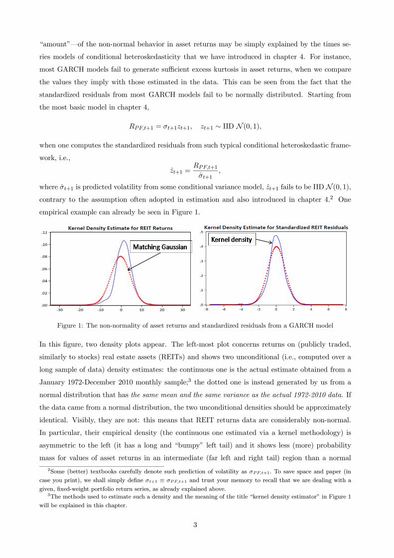
Figure 1: The non-normality of asset returns and standardized residuals from a GARCH model
In this figure, two density plots appear. The left-most plot concerns returns on (publicly traded,
similarly to stocks) real estate assets (REITs) and shows two unconditional (i.e., computed over a
long sample of data) density estimates: the continuous one is the actual estimate obtained from a
January 1972-December 2010 monthly sample;3 the dotted one is instead generated by us from a
normal distribution that has the same mean and the same variance as the actual 1972-2010 data. If
the data came from a normal distribution, the two unconditional densities should be approximately
identical. Visibly, they are not: this means that REIT returns data are considerably non-normal.
In particular, their empirical density (the continuous one estimated via a kernel methodology) is
asymmetric to the left (it has a long and “bumpy” left tail) and it shows less (more) probability
mass for values of asset returns in an intermediate (far left and right tail) region than a normal
2Some (better) textbooks carefully denote such prediction of volatility as +1 To save space and paper (in
case you print), we shall simply define +1 ≡ +1 and trust your memory to recall that we are dealing with a
given, fixed-weight portfolio return series, as already explained above.3The methods used to estimate such a density and the meaning of the title “kernel density estimator” in Figure 1
will be explained in this chapter.
3

density does. We say that asset returns are asymmetrically distributed and leptokurtic; the latter
feature implies that their tails (often, especially the left one, where large losses are recorded) are
“fatter” than under a normal benchmark.
The right-most plot contains similar, but less extreme evidence, and no longer concerns raw
REIT asset returns: the second plot concerns instead the standardized residuals originated from
fitting a Gaussian GARCH(1,1) model (with leverage, say in a GJR fashion) on REIT returns:
+1 =
+1 +1 . As already stated, if the Gaussian GARCH(1,1) model were correctly
specified, then the hypothesis that +1 ∼ IID N (0 1) should not be rejected. The right-most
plot in Figure 1 shows however that this is not the case: the continuous, kernel density estimator
remains visibly different from the dotted one, obtained also in this case from a normal distribution
that has the same mean and the same variance as the estimated standardized residuals for the
January 1972 - December 2010 sample. In Figure 1, even after estimating a GARCH, the resulting
standardized residuals remain non-normal: their empirical density is asymmetric to the left (because
of that bump that you can detect around -4 standard deviations on the horizontal axis) and it shows
less (more) probability mass for values of asset returns in an intermediate (far left and right tail)
region than a normal density does. Also standardized REIT returns from the GARCH(1,1) model
are asymmetric and leptokurtic.
These results tends to be typical for most financial return series sampled at high (e.g., daily or
weekly) and intermediate frequencies (monthly, as in Figure 1). For instance, stock markets exhibit
occasional, very large drops but not equally large up moves. Consequently, the return distribution
is asymmetric or negatively skewed. However, some markets such as that for foreign exchange tend
to show less evidence of skewness. For most asset classes, in this case including exchange rates,
return distributions exhibit fat tails, i.e., a higher probability of large losses (and gains) than the
normal distribution would allow.
Note that Figure 1 is not only bad news: the improvement when one moves from the left to
the right is obvious. Even though we lack at the moment a formal way to quantify this impression,
it is immediate to observe that the “amount” of non-normalities declines when one goes from
the raw (original) REIT returns (+1 ) to the Gaussian GARCH-induced standardized residuals
(+1 ≡
+1 +1 ). Yet, the improvement is insufficient to make the standardized
residuals normally distributed, as the model assumes. In this chapter, we also ask how the GARCH
models introduced in chapter 4 can be extended and improved to deliver unconditional distributions
that are distributed in the same way as their original assumptions imply.
3. Testing and Measuring Deviations from Normality
In this section, we develop statistical tools to perform tests of non-normality applied to an empirical
density (of either returns or standardized residuals). We also provide a quick primer to methods
of estimation of empirical densities, to try and “quantify” any such deviations from a Gaussian
4

benchmark.
The key tool to perform statistical tests of normality is Jarque and Bera’s (1980) test.4 The test
has a very intuitive structure and is based on a simple fact: if ∼ N ( 2), then the distributionof is symmetric–therefore it has zero skewness–and it has a kurtosis of 3.
5 In particular, if we
define the unconditional mean ≡ [] and the variance 2 ≡ [] then skewness is
[] ≡ [( − )3]
( [])32=
[( − )3]
3
while kurtosis is6
[] ≡ [( − )4]
( [])2=
[( − )4]
4≥ 0
Clearly, skewness is the scaled third central moment, while kurtosis is the scaled fourth central
moment.7 When skewness is positive (negative), then [( − )3] 0 ( 0) and this means
that there is a larger probability mass below (above) the mean than there is above (below).
Because a normal distribution implies perfect symmetry around the mean and therefore the same
probability below and above then [] = 0 when ∼ N ( 2) We also call excesskurtosis the quantity [] − 3 which derives from the fact that [] = 3 when ∼N ( 2) A positive (negative) excess kurtosis implies that has fatter (thinner) tails than a
normal distribution. Because [] ≥ 0 then excess kurtosis may at most be equal to -3.Jarque and Bera’s test is based on sample estimates of skewness and (excess kurtosis) from the
data, here either raw asset returns or standardized residuals from an earlier estimation of some
dynamic econometric model. Denoting with a “hat” sample estimates of central moments obtained
from the data, under the null hypothesis of normally distributed errors, Jarque and Bera’s test
statistic is: d ≡
6
n\[]
o2+
24
n[[]− 3
o2 ∼ 22
where is sample size, and the pedix 2 in 22 indicates that the critical value needs to be found
under a chi-square distribution with 2 degrees of freedom. As usual, large values of this statistic–
exceeding some critical value under the 22 selected for a given size (i.e., probability of a type I error)
of the test–will indicate departures from normality. Note thatd is a function of excess kurtosis
4This is not the only test available, but it is certainly the most widely used in applied finance.5Here is any generic time series. In this chapter, we shall be interested in two cases: when = and
when = from some model. In the second case, when we deal with standardized residuals, we shall ignore the fact
that depends on some vector of estimated parameters, ; to take that into account would introduce considerable
complications because it would make each a function of the entire data sample, {}=1. This occurs because theentire data set {}=1 has been presumably used to estimate .
6Later skewness will also be called 1 and excess kurtosis 2.7A central moment is defined as ≡ [( − )] where is an integer number. Skewness and kurtosis are
scaled central moments because they are divided by This derives from the desire to express skewness and kurtosis
as pure numbers, which is obtained by dividing them by another central moment (here the second), raised to the
appropriate power so that the unit of measurement at the numerator and denominator (e.g., percentage) exactly
cancel out. The fact that skewness and kurtosis are pure numbers means that these can be compared across different
series, different periods, etc. Because kurtosis is the ratio of two (powers) of positive central moments, then it can
only be non-negative.
5

and not of kurtosis only. This result derives from the fact thatd is the sum of the squares of two
random variables (technically, sample statistics) that have each a normal asymptotic distribution,8
√\[]
∼ N (0 6)√n[[]− 3
o∼ N (0 24)
are also asymptotically independently distributed.
For instance, using daily returns S&P 500 data for the sample period 1926-2010, we have:
Figure 2: The non-normality of daily S&P 500 returns
The Jarque-Bera statistic in this case is huge: 273,195 which is well above any critical values under
a 22 (e.g., these are 5.99 for = 5%; 9.21 for = 1%; 13.82 for = 01%)! Clearly, the null
hypothesis of U.S. stock returns being normally distributed can be rejected at any significance level;
in fact, the p-value associated with such a large value of d is essentially zero. This rejection of
the null hypothesis of normality derives from a very large excess kurtosis of 17.16, in spite of a
negligible skewness of -0.007 only. Note that
22 276
24{1716}2 ' 273 313
is very close to the total d statistic of 273,195, with the difference only due to rounding. Once
more also the right-most plot in Figure 2 emphasizes that S&P 500 daily returns are not normally
distributed, see the differences between the continuous, kernel density estimator and the dotted one,
obtained also in this case from a normal distribution that has the same mean and the same variance
as the daily stock returns in the sample.
Once more, whilst commenting Figure 2 we have used the notion that the unconditional density
of S&P 500 daily returns has been estimated using some “kernel density estimator”: it is about
time to clarify what this entails. A kernel density estimator is an empirical density “smoother”
based on the choice of two objects: (i) the kernel function () and (ii) the bandwidth parameter,
. The kernel function is defined as some smooth function (read, continuous and sometimes also
8It is well known that if ∼ N ( 2) = 1 2 ..., and are independent, then 21 + 2
2 + 2 + 2
∼ 2.
The notation∼ D means that asymptotically, as →∞, the distribution of the statistic under examination is D.
6

differentiable) that integrates to 1: Z +∞
−∞ () = 1
For instance, a typical kernel function is the Gaussian one,
() =1√2
−122 (1)
which also corresponds to the probability density function of a N (0 1) variate (right?). Here
represents any possible value that the generic random variable may take.9 The bandwidth
parameter is instead used to allocate weight to values of in the support of that differ from
a given . This last claim can be understood only by inspecting the general definition of a kernel
density estimator :
ker () =1
X=1
µ−
¶ (2)
where is the number of points over which the estimation is based, usually the size of the sample
at hand (in this case, = ). Two aspects need to be adequately emphasized. First, in (2) we are
estimating not a parameter of the population (such as the mean, the variance, the slope coefficient
in a regression or the GARCH coefficients as it happened in chapter 4), but the entire density
of such a population. This means that ker () represents an estimator of the true but unknown
().10 Second, the mechanics of (2) is easy to understand: for each in your data set, you
compute ker () for any arbitrary value in the support of , by running through your entire
sample, computing for each the kernel “scores” ((− )) and summing them. Note that
because you have observations in your sample and the differences (− ) are re-weighted by the
bandwidth the total sum is scaled by the factor . In this sense, note that a large (small)
tends to strongly (weakly) shrink any ( − ) 6= 0, which justifies our claim that the bandwidth
parameter allocates weight to values of in the support of that differ from a given .
As esoteric as this may sound, the truth is that since the early ages you have been implicitly
trained to compute and use kernel density estimators all the time. As it often occurs however, you
have also been educated to use a very poor–in a statistical sense–kernel density estimator, the
so-called “histogram estimator” that is obtained from the general formula in (2) when = 1 (as we
shall see, = 1 is hardly optimal) and the kernel function is Dirac (usually denoted as ()), i.e.,
9Generic, because we are still trying to deal with both the case of asset or portfolio returns, = and with
= from some model.10Yes, it is possible. In case you are asking yourselves what is the point of spending years studying how to estimate
parameters of such a population density while one may actually attack the problem by estimating the density itself,
don’t. The branch of statistics that deals with the second task is called nonparametric statistics (econometrics).
Although its goals are as general as ambitious, these do not solve all the problems that applied finance people
usually face. For instance, in finance we care a lot for not only fitting/modelling objects of interest, but also in
understanding their dynamics over time (because we would like to predict them). Nonparametric econometrics becomes
very problematic when it is employed in view of this second type of objective. Hence parametric econometrics remains
a crucial subject and most work in applied finance and economics is still organized around parametric methods.
7

a sort of indicator function:
(− ) = () =
(1 if =
0 if 6=
As a result, every time you build a histogram and you try and go around showing off, you are
using:11
() =1
X=1
( = ) = Fraction of your data equal to .
Of course, there is no good reason to set (− ) = () or = 1. On the contrary, after the
naive histogram estimator, the most common type of kernel function used in applied finance is the
Gaussian kernel in (1). A () with optimal (in a Mean-Squared Error sense) properties is instead
Epanechnikov’s:
() =3
4√5
¡1− 022¢ (−√5 ≤ ≤
√5) (3)
Other popular kernels are the triangular and box kernels:
() =1
2(|| 1) () = (1− ||)(|| 1) (4)
Figure 3 shows the kernels in (3) and (4) (I guess you can easily picture the shape of a box on your
own, just think of when you buy shoes):
Figure 3: The Epanechnikov (left) and Triangular (right) kernels
The fact that Epanechnikov’s kernel is optimal–because it minimizes the average squared deviations
[() − ker ()]2–while the Gaussian is not, illustrates one general point, that to minimize the
integrated MSE,
Z +∞
−∞[()− ker ()]2
kernel functions that are truncated and do not extend to the infinite right and left tails tend to
display superior properties when compared to kernels that do. However, the histogram kernel over-
does it in this dimension and seems to excessively truncate, because it prevents that any 6=
11Usually, what we do to present smarter-looking results, is to organize the possible values of in buckets (intervals)
and estimate the probability of that interval as the percentage of your sample that falls in that bucket. However, the
nature of the resulting density estimator is the same, alas. In the following formula, note that ( = ) and {=}have the same meaning.
8

may bring any information useful to the estimation of (). Finally, the bandwidth parameter
is usually chosen according to the rule ( here is again the sample size):
= 09 · · −15
which minimizes the integrated MSE across kernels.
How does one use kernel density estimators and do different choices of() make a big difference
when it comes to assess deviations from normality? The first question has a trivial answer: here
we are in the notoriously difficult (and silly) “eyeballing domain” and–as we did above in our
comments–every time one notices large departures of the kernel density estimates from a given
benchmark (for us, the normal distribution, also called Gaussian by the educated people), you have
legitimation to debate the issue, and especially how and why the deviation occurs. However, it is
doubtful that the choice of optimal vs. sub-optimal kernel density estimators may make a first-order
differences for our ability to assess whether data are normal or not. For instance, in Figure 4, it
seems that financial returns (in this case, value-weighted U.S. stock returns) are easily assessed to
be leptokurtic, i.e., they have fat tails and highly peaked densities around the mean, independently
of the specific kernel density estimator that is employed.
Moment‐matchedGaussian
Figure 4: The non-normality of monthly U.S. stock returns using three alternative kernel density estimators
If you are ready to work with visual tools instead of performing formal inference on the null
hypothesis of normally distributed returns or standardized residuals, another informal and yet
powerful method to visualize non-normalities consists of quantile-quantile (Q-Q) plots. The idea is
to plot in a standard Cartesian reference graph:
• the quantiles of the series under consideration, , either raw returns or standardized residuals
from the earlier fit of some conditional econometric model;
• against the quantiles of the normal distribution.
If the returns were truly normal, then the graph should look like a straight line with a 45-
degree angle. The reason is that if the theoretical (in this case, normal) and empirical quantiles
are exactly identical, then they must fall on the 45-degree line. Systematic deviations from the
45-degree line signal that the returns are not well described by the normal distribution and give
9
ground to rejection of the null of normality. The recipe to build a Q-Q plot is simple: first, sort
all (standardized) returns in ascending order, and call the th sorted value ; second, compute
the empirical probability of getting a value below the actual as ( − 05) , where is number
of observations available in the sample.12 Finally, we calculate the standard normal quantiles as
Φ−1 ((− 05) ) where Φ−1 (·) denotes the inverse of a standard normal density. At this point, wecan represent on a scatter plot the (standardized) returns and sort the data on the Y-axis against
the standard normal quantiles on the X-axis. Figure 5 shows two examples of Q-Q plots applied to
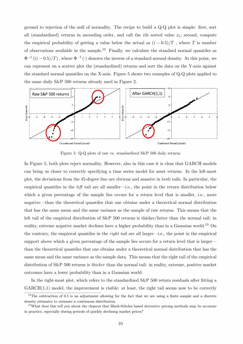
the same daily S&P 500 returns already used in Figure 2.
Raw S&P 500 returns After GARCH(1,1)
Figure 5: Q-Q plots of raw vs. standardized S&P 500 daily returns
In Figure 5, both plots reject normality. However, also in this case it is clear that GARCH models
can bring us closer to correctly specifying a time series model for asset returns. In the left-most
plot, the deviations from the 45-degree line are obvious and massive in both tails. In particular, the
empirical quantiles in the left tail are all smaller–i.e., the point in the return distribution below
which a given percentage of the sample lies occurs for a return level that is smaller, i.e., more
negative–than the theoretical quantiles that one obtains under a theoretical normal distribution
that has the same mean and the same variance as the sample of raw returns. This means that the
left tail of the empirical distribution of S&P 500 returns is thicker/fatter than the normal tail: in
reality, extreme negative market declines have a higher probability than in a Gaussian world.13 On
the contrary, the empirical quantiles in the right tail are all larger–i.e., the point in the empirical
support above which a given percentage of the sample lies occurs for a return level that is larger–
than the theoretical quantiles that one obtains under a theoretical normal distribution that has the
same mean and the same variance as the sample data. This means that the right tail of the empirical
distribution of S&P 500 returns is thicker than the normal tail: in reality, extreme, positive market
outcomes have a lower probability than in a Gaussian world.
In the right-most plot, which refers to the standardized S&P 500 return residuals after fitting a
GARCH(1,1) model, the improvement is visible: at least, the right tail seems now to be correctly
12The subtraction of 0.5 is an adjustment allowing for the fact that we are using a finite sample and a discrete
density estimator to estimate a continuous distribution.13What does this tell you about the chances that Black-Scholes based derivative pricing methods may be accurate
in practice, especially during periods of quickly declining market prices?
10

modeled by the GARCH. However, even if these are now less obvious, the problems in the left tail
remain. This means that a simple, plain-vanilla GARCH(1,1) model with Gaussian shocks,
&+1 = (
q + (&
)2 + 2 )+1 +1 ∼ IID N (0 1)
cannot completely handle the empirical thickness of the tails of S&P 500 returns.14 Finally, let’s
ask: why do risk managers care of Q-Q plots? Because differently from the JB test and kernel
density estimators, Q-Q plots provide visual–usually, rather clear–information on where (in the
support of the empirical return distribution) non-normalities really occur. This is an important
pointer to ways in which a model may be extended or amended to provide a better fit and hence,
more accurate forecasts.
4. t-Student Distributions for Asset Returns
An obvious question is then: if all (most) financial returns have non-normal distributions, what can
we do about it? More importantly, this question can be re-phrased as: if most financial series yield
non-normal standardized residuals even after fitting many (or all) of the GARCH models analyzed in
chapter 4, that assume that such standardized residuals ought to have a Gaussian distribution, what
can be done? Notice one first implication of these very questions: especially when high-frequency
(daily or weekly) data are involved, we should stop pretending that asset returns “more or less” have
a Gaussian distribution in many applications and conceptualizations that are commonly employed
outside econometrics: unfortunately, it is rarely the case that financial returns do exhibit a normal
distribution, especially if sampled at high frequencies (over short horizons).15
When it comes to find remedies to the fact that plain-vanilla, Gaussian GARCH models cannot
quite capture the key properties of asset returns, there are two main possibilities that have been
explored in the financial econometrics literature. First, to keep assuming that asset returns are
IID, but with marginal, unconditional distributions different from the Normal; such marginal dis-
tributions will have to capture the fat tails and possibly also the presence of asymmetries. In this
chapter we introduce the leading example of the -Student distribution. Second, to stop assuming
that asset returns are IID and model instead the presence of rich–richer than it has been done in
chapter 4–dynamics/time-variation in their conditional densities. But we have done that already
on a rather extensive scale in chapter 4–where ARCH and GARCH models have been introduced
and several variations considered–and we have already seen a few examples of how such a strategy
14Augmenting this model to include simple asymmetric effects (as in the GJR case) improves its fit, but does not
make the rest of our discussion moot.15One of the common explanations for the financial collpse of 2008-2009, is that many prop trading desks at major
international banks had uncritically downplayed the probability of certain extreme, systematic events. One reason
for why this may happen even when a quant is applying (seemingly) sophisticated techniques is that Gaussian shocks
were too often assumed to represent a sensible specification, ignoring instead the evidence of jumps and non-normal
shocks. Of course, this is just one aspect of why so many international institutions found themselves at a loss when
faced with the events of the Fall and the Winter of 2008/09.
11
may represent an important and fun first step, but that this may be often insufficient to capture all
the salient features of the data. Indeed, it turns out that both approaches are needed by high fre-
quency (e.g., daily) financial data, i.e., one needs ARCH and GARCH models extended to account
for non-normal innovations (see e.g., Bollerslev, 1987).
Perhaps the most important type of deviation from a normal benchmark for (or ) are
the fatter tails and the more pronounced peak around the mean (or the model) for (standardized)
returns distribution as compared with the normal one, see Figures 1, 2, and 4. Assume the instead
that financial returns are generated by
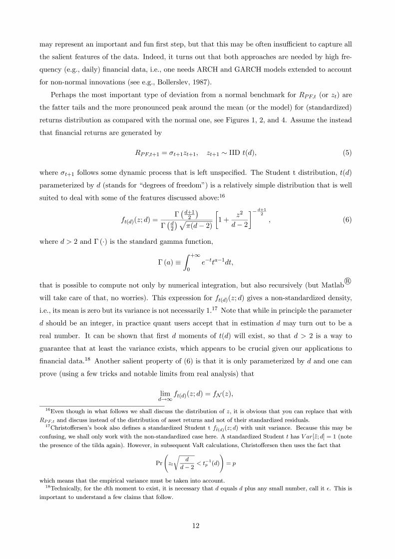
+1 = +1+1 +1 ∼ IID () (5)
where +1 follows some dynamic process that is left unspecified. The Student t distribution, ()
parameterized by (stands for “degrees of freedom”) is a relatively simple distribution that is well
suited to deal with some of the features discussed above:16
()(; ) =Γ¡+12
¢Γ¡2
¢p(− 2)
∙1 +
2
− 2¸− +1
2
(6)
where 2 and Γ (·) is the standard gamma function,
Γ () ≡Z +∞
0
−−1
that is possible to compute not only by numerical integration, but also recursively (but MatlabR°
will take care of that, no worries). This expression for ()(; ) gives a non-standardized density,
i.e., its mean is zero but its variance is not necessarily 1.17 Note that while in principle the parameter
should be an integer, in practice quant users accept that in estimation may turn out to be a
real number. It can be shown that first moments of () will exist, so that 2 is a way to
guarantee that at least the variance exists, which appears to be crucial given our applications to
financial data.18 Another salient property of (6) is that it is only parameterized by and one can
prove (using a few tricks and notable limits from real analysis) that
lim→∞
()(; ) = N ()
16Even though in what follows we shall discuss the distribution of it is obvious that you can replace that with
and discuss instead of the distribution of asset returns and not of their standardized residuals.17Christoffersen’s book also defines a standardized Student t ()(; ) with unit variance. Because this may be
confusing, we shall only work with the non-standardized case here. A standardized Student has [; ] = 1 (note
the presence of the tilda again). However, in subsequent VaR calculations, Christoffersen then uses the fact that
Pr
− 2 −1 ()
=
which means that the empirical variance must be taken into account.18Technically, for the th moment to exist, it is necessary that equals plus any small number, call it . This is
important to understand a few claims that follow.
12

as diverges, the Student- density becomes identical to a standard normal. This plays a practical
role: even though you assume that (6) holds, if estimation delivers a rather large (say, above 20,
just to indicate a threshold), this will represent indication that either the data are approximately
normal or that (6) is inadequate to capture the type of departure from normality that you are after.
What could that be? This is easily seen from the fact that in the simple case of a constant variance,
(6) is symmetric around zero, and its mean, variance, skewness (1), and excess kurtosis (2) are:
[; ] = = 0 [; ] = 2 =
− 2[; ] = 1 = 0 [; ] = 2 =
6
− 4 (7)
The skewness of (6) is zero (i.e., the Student is symmetric around the mean), which makes it
unfit to model asymmetric returns: this is the type of departure from normality that (6) cannot yet
capture and no small can be used to accomplish this.19
The key feature of the () density is that the random variable, , is raised to a (negative) power,
rather than a negative exponential, as in the standard normal distribution:
N () =1√2
−122
This allows () to have fatter tails than the normal, that is, higher values of the density ()(; )
when is far from zero. This occurs because the negative exponential function is known to decline
to zero (as the argument goes to infinity, in absolute value) faster than negative power functions
may ever do. For instance, observe that for = 4 (which may be interpreted as meaning four
standard deviations away from the mean) while
−1242 = 00003355
under a negative power function with = 10 (later you shall understand the reason of this choice),∙1 +
42
8
¸−112
= 00023759
Notice that the second probability value is (0.0023759/0.0003355) = 7.08 times larger. If you repeat
this experiment considering a really large, extreme realization, say some (standardized) return 12
times away from the sample mean (say a -9.5% return on a given day), then exp(−05 · 122) =53802−32 which is basically zero (impossible, but how many -10% did we really see in the Fall of
2008?), while ∙1 +
122
8
¸− 112
= 92652−8
19Let’s play (as we shall in do in the class lectures): what is the excess kurtosis of the t-student if = 3? Same
question when = 4. What if instead = 400001 (which is 4 plus that small mentioned in a previous footnote)?
Does the intution that as →∞ the density becomes normal fit with the expression for 2 reported above?
13

Although also the latter number is rather small,20 the ratio between the two probability assessments
(92652−853802−32) is now astronomical (1.72224): events that are impossible under a Gaussian
distribution become rare but billions of times more likely under a fat-tailed, t-Student distribution.
This result is interesting in the light of the comments we have expressed about the left tail of the
density of standardized residuals in Figure 5.
In this section, we have introduced (6) as a way to take care of the fact that, even after fit-
ting rather complex GARCH models, (standardized) returns often seemed not to conform to the
properties–such as zero skewness and zero excess kurtosis–of a normal distribution. How do you
now assess whether the new, non-normal distribution assumed for actually comes from a Student
? In principle, one can easily deploy two of the methods reviewed in Section 3 and apply them to
the case in which we want to test the null of IID (): first, extensions of Jarque-Bera exist to
formally test whether a given sample has a distribution compatible with non-normal distributions,
e.g., Kolmogorov-Smirnov’s test (see Davis and Stephens, 1989, for an introduction); second, in
the same way in which we have previously informally compared kernel density estimates with a
benchmark Gaussian density for a series of interest, the same can be accomplished with reference
to, say, a Student- density. Finally, we can generalize Q-Q plots to assess the appropriateness of
non-normal distributions. For instance, we would like to assess whether the same S&P 500 daily
returns standardized by a GARCH(1,1) model in Figure 5 may actually conform to a t() distri-
bution in Figure 6. Because the quantiles of t() are usually not easily found, one uses a simple
relationship with a standardized () distribution, where the tilde emphasizes that we are referring
to a standardized t:
Pr
à −1 ()
r− 2
!= Pr
¡ −1 ()
¢where the critical values of −1 () are tabulated. Figure 6 shows that assuming -Student conditional
distributions may often improve the fit of a GARCH model.
After GARCH(1,1) After t‐GARCH(1,1)
Figure 6: Q-Q plots of Gaussian vs. t-Student GARCH(1,1) standardized S&P 500 daily returns
Although some minor issues with the left tail of the standardized residuals remain, many users
20Please verify that such probability increases becoming not really negligible if you lower the assumption of = 10
towards = 2
14

may actually judge the right-most QQ plot as completely satisfactory and favorable to a Student
GARCH(1,1) model capturing the salient features of daily S&P 500 returns.
4.1. Estimation: method of moments vs. (Q)MLE
We can estimate the parameters of (5)–when we estimate (6) directly on the standardized residuals,
we can speak of only–using MLE or the method of moments (MM). As you know from chapter
4, in the MLE case, we will exploit knowledge (real or assumed) of the density function of the
(standardized) residuals. Nothing needs to be added to that, apart the fact that the functional
form of the density function to be assumed is now given by (6). The method of moments relies
instead on the idea of estimating any unknown parameters by simply matching the sample moments
in the data with the theoretical (population) moments implied by a t-Student density. The intuition
is simple: if the data at hand came from the Student-t family parameterized by , and 2 (say),
then the best among the members of such a family will be characterized by a choice of and
2 that generates population moments that are identical or at least close to the observed sample
moments in the data.21 Technically, if we define the non-central and central sample moments of
order ≥ 1 (where is a natural number) as22
≡ 1
X=1
() b ≡ 1
X=1
( − 1)
respectively, in the case of (5), it is by equating sample and theoretical moments that we get the
following system to be solved with respect to the unknown parameters:
= 1 (population mean = sample mean)
2
− 2 = b2 (population variance = sample variance)
2 =6
− 4 =b4 − 3b2
2
(population excess kurtosis = sample excess kurtosis).
Note that all quantities on the right-hand side of this system will turn into numbers when you are
given a sample of data. Why these 3 moments? They make a lot of sense given our characterization
of (5)-(6) and yet, these are selected, by us, rather arbitrarily (see below). This is a system of 3
21In what follows, we will focus on the simple case in which is itself a constant and as such it directly becomes
one of the parameters to be estimated. This means that (5) is really considered to be+1 = ++1 +1 ∼IID() where a mean parameter is added, just in case.22Notice that sample moments are sample statistics because they depend on a random sample and as such they
are estimators. Instead the population moments are parameters that characterize the entire data generating process.
Clearly, 1 = = [], while 2 = []. The expressions that follow still refer to but there is little problemin extending them to raw portfolio returns (, as in the lectures) or to any other time series.
15

equations in 3 unknown (with a recursive block structure) that is easy to solve to find:23
= 4 +64
( 2)2− 3
2 = b2 − 2
= 1
In practice, one first goes from the sample excess kurtosis to estimate the number of degrees of
freedom of the Student , ; then to the estimate of the variance coefficient (also called diffusive
coefficient), and finally as well as independently, to compute an estimate of the mean (which is
just the sample mean). Interestingly, while under MLE we are used to the fact that one possible
variance estimator is 2 = b2 in the case of MM applied to the t-Student, we have
2 = b2 − 2
2
because ( − 2) 1 for any 2. This makes intuitive sense because in the case
of a t-Student, the variability of the data is not only explained by their “pure” variance, but also
by the fact that their tails are thicker than under a normal: as → 2 (from the right), you
see that ( − 2) goes to zero, so that for given b2, 2 can be much smaller than the
sample variance; in that case, most of the variability in the data does come from the thick tails of
the Student . On the contrary, as →∞ we know that this means that the Student becomes
indistinguishable from a normal density, and as such we have that ( − 2) → 1 and
2 → b2 = 2.24 Additionally, note that as intuition would suggest, as 2 ≡ ( b4( b2)
2)− 3gets larger and larger, then
lim2→∞
= lim2→∞
4 +6
2= 4
where 4 represents the limit of the minimal value for that one may have with the fourth central
moment remaining well-defined under a Student . Moreover, based on our earlier discussion, we
have that
lim2→0
= lim2→0
4 +6
2= +∞
which is a formal statement of the fact that a Student distribution fitted on data that fail to
exhibit fat tails, ought to simply become a normal distribution characterized by a diverging number
of degrees of freedom, . Finally, MM uses no information on the sample skewness of the data for
a very simple reason: as we have seen, the Student in (6) fails to accommodate any asymmetries.
Besides being very intuitive, is MM a good estimation method? Because MM does not exploit
the entire empirical density of the data but only a few sample moments, it is clearly not as efficient
as MLE. This means that the Cramer-Rao lower bound–the maximum efficiency (the smallest
23In the generalized MM case (called GMM) in which one has more moments than parameters to estimate, it will
be possible to select weighting schemes across different moments that guarantee that GMM estimators may be as
efficient as MLE ones. But this is an advanced topic, good for one of your electives.24Even though at first glance it may look so, please do not use this example to convince yourself that MLE only
works when the data are normally distributed. This is not true (under MLE one needs to know or assume the density
of the data, and this can be also non-normal).
16
covariance matrix of the estimators) that any estimator may achieve–will not be attained. Prac-
tically, this means that in general MM tends to yield standard errors that are larger than those
given by MLE. In some empirical applications, for instance when we are assessing models on the
basis of tests of hypotheses of some of their parameter estimates, we shall care for standard errors.
This result derives from the fact that while MLE exploits knowledge of the density of the data,
MM does not, relying only on a few, selected moments (as a minimum, these must be in a number
identical to the parameters that need to be estimated). Because while the density () (or the CDF
()) has implications for all the moments (an infinity of them), but the moments fail to pin down
the density function–equivalently, () =⇒ (), but the opposite does not hold so that it
is NOT true that () ⇐⇒ ()–MM potentially exploits much less information in the data
than MLE does and as such it is less efficient.25
Given these remarks, we could of course estimate also by MLE or QMLE. For instance,
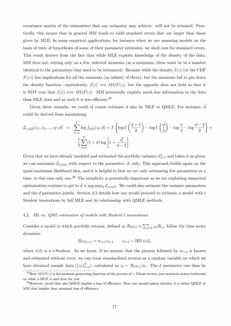
could be derived from maximizing
L1()(1 2 ; ) =
X=1
log ()(; ) =
½logΓ
µ+ 1
2
¶− logΓ
µ
2
¶− log
2− log − 2
2
¾+
−12
X=1
(1 + ) log
∙1 +
2− 2
¸
Given that we have already modeled and estimated the portfolio variance 2+1 and taken it as given,
we can maximize L1() with respect to the parameter, , only. This approach builds again on thequasi-maximum likelihood idea, and it is helpful in that we are only estimating few parameters at a
time, in this case only one.26 The simplicity is potentially important as we are exploiting numerical
optimization routines to get to ≡ argmax L1(). We could also estimate the variance parametersand the parameter jointly. Section 4.2 details how one would proceed to estimate a model with
Student innovations by full MLE and its relationship with QMLE methods.
4.2. ML vs. QML estimation of models with Student innovations
Consider a model in which portfolio returns, defined as ≡P
=1 , follow the time series
dynamics
+1 = +1+1 +1 ∼ IID ()
where () is a t-Student. As we know, if we assume that the process followed by +1 is known
and estimated without error, we can treat standardized returns as a random variable on which we
have obtained sample data ({}=1), calculated as = . The parameter can then be
25Here () is the moment generating function of the process of Please review your statistics notes/textbooks
on what a MGF is and does for you.26However, recall that also QMLE implies a loss of efficiency. Here one should assess whether it is either QMLE or
MM that implies that mimimal loss of efficiency.
17

estimated using MLE by choosing the which maximizes:27
L1()(1 2 ; ) =
X=1
ln (; ) =
X=1
lnΓ¡+12
¢Γ¡2
¢p(− 2) −
1 +
2
X=1
ln
µ1 +
2− 2
¶= lnΓ
µ+ 1
2
¶− lnΓ
µ
2
¶− 12 ln − 1
2 ln(− 2)+
−1 +
2
X=1
ln
µ1 +
2− 2
On the contrary, if you ignored the estimate of either (if it were a constant) or of the process
for +1 (e.g., a GARCH(1,1) process) and yet you proceeded to apply the method illustrated
above (incorrectly) taking some estimate of either or of the process for +1 as given and free of
estimation error, you would obtain a QMLE estimator of . As already discussed in chapter 4, QML
estimators have two important features. First, they are not as efficient as proper ML estimators
because they ignore important information on the stochastic process followed by the estimator(s)
of either or of the process followed by +1.28 Second, QML estimators will be consistent and
asymptotically normal only if we can assume that any dynamic process followed by +1 has been
correctly specified. Practically, this means that when one wants to use QML, extra care should
be used in making sure that a “reasonable” model for +1 has been estimated in the first step,
although you see that what may be reasonable is obviously rather subjective.
If instead you do not want to ignore the estimated nature of the process for +1 and proceed
instead to full ML estimation, for instance when portfolio variance follows a GARCH(1,1) process,
2 = + 2−1 + 2−1
the joint estimation of , , , and implies that the density in the lectures,
(; ) =Γ¡+12
¢Γ¡2
¢p(− 2)
µ1 +
2− 2
¶−1+2
,
must be replaced by
(; ) =Γ¡+12
¢Γ¡2
¢p(− 2)2
µ1 +
()2
− 2¶− 1+
2
where the 2 in
Γ¡+12
¢Γ¡2
¢p(− 2)2
27Of course, MatlabR°will happily do this for you. Please see the Matlab workout in Appendix B. See also the
Excel estimation performed by Christoffersen (2012) in his book. Note that the constraint 2 will have to be
imposed.28In particular, you recognize that either or the process of +1 will be estimated with (sometimes considerable)
uncertainty (for instance, as captured by the estimate standard errors), but none of this uncertainty is taken into
account by the QML maximization. Although the situation is clearly different, it is logically similar to have a sample
of size but to ignore a portion of the data available: that cannot be efficient. Here you would be potentially ignoring
important sample information that the data are expressing through the sample distribution of either or the process
of +1.
18

comes from (; ) = () so that (; ) = () (this is called the Jacobian of the
transformation, please review your Statistics notes or textbooks). Therefore, the ML estimates of
, , , and will maximize:
L2()(1 2 ; ) =
X=1
log (; ) =
X=1
log
⎧⎨⎩ Γ¡+12
¢Γ¡2
¢q(− 2)( + 2−1 + 2−1)
Ã1 +
2
(− 2)( + 2−1 + 2−1)
!−1+2
⎫⎬⎭
(8)
This looks very hard because the parameters enter in a highly non-linear fashion. Of course
MatlabR°can take care of it, but there is a way you can get smart about maximizing (8). Define
≡ q + 2−1 + 2−1. Call L1()() the likelihood function when the standard-
ized residuals are the s and L2()
( ) the full log-likelihood function defined above. It
turns out that L2()
( ) may be decomposed as
L2()( ) = L1()()−1
2
X=1
ln( + 2−1 + 2−1)
This derives from the fact that in (8),
L2()( ) = lnΓ
µ+ 1
2
¶− lnΓ
µ
2
¶− 12 ln − 1
2 ln(− 2) +
−12
X=1
ln( + 2−1 + 2−1)−1 +
2
X=1
ln
∙1 +
( )2
− 2¸
= L1()()−1
2
X=1
ln( + 2−1 + 2−1)
This decomposition helps us in two ways. First, it shows exactly in what way the estimation
approach simply based on the maximization of L1()
() is at best a QML one:
argmax
L1()() ≤ argmax
"L1()()−
1
2
X=1
ln( + 2−1 + 2−1)
#
This follows from the fact that the maximization problem on the right-hand side also exploits the
possibility to select the GARCH parameters , , and , while the one of the left-hand side does
not. Second, it suggests a useful short-cut to perform ML estimation, especially under a limited
computational power:
• Given some starting candidate values for [ ]0 maximize L1()
() to obtain (1);
• Given (1), maximize L1()()− 12
P=1 ln(+2−1+2−1) by selecting [(1) (1) (1)]
0
and computen(1) ≡
q(1) + (1)
2−1 + (1)
2−1o=1;
• Given [(1) (1) (1)]0 maximize L1()() to obtain (2);
19

• Given (2), maximize L(2)1()((2))− 1
2
P=1 ln( + 2−1 + 2−1) by selecting [(2) (2)
(2)]0 and compute
n(2) ≡
q(1) + (1)
2−1 + (1)
2−1o=1.
At this point, proceed iterating following the steps above until convergence is reached on the
parameter vector [ ]0.29 What is the advantage of proceeding in this fashion? Notice that you
have replaced a (constrained) optimization in 4 control variables ([ ]0) with an iterative process
in which there is a constrained optimization in 1 control followed by a constrained optimization in
3 controls. These may seem small gains, but the general principle may find application to cases
more complex than a t-Student marginal density of the shocks, in which more than one additional
parameter (here ) may be featured.
4.3. A simple numerical example
Consider extending the moment expressions in (7) to the simple time homogeneous dynamics
= + ∼ IID (). (9)
Because we know that if ∼ IID () then [] = 0, [] = ( − 2), [] = 0, and
[] = 3 + 6(− 4), it follows that
[] = + [] =
[] = 2 [] =
− 22
[( −[])3] = 3[3 ] = 0
() ≡ [( −[])4]
( [])2
=4
4( [])2[4 ] =
[4 ]
( [])2= () = 3 +
6
− 4
Interestingly, while mean and variance are affected by the structure of (9), skewness and kurtosis,
being standardized central moments, are not.
Clearly, if you had available sample estimates for mean, variance, and kurtosis from a data set
of asset returns defined as
1 ≡ 1 =1
X=1
, 2 ≡ 1
X=1
( − 1)2, 4 ≡ 1
X=1
( − 1)4
4
(2)2=
P=1( − 1)
4hP=1( − 1)2
i2 it would be easy to recover an estimate of from sample kurtosis, an estimate of 2 from sample
variance, and an estimate of from the sample mean. Using the method of moments, we have
29For instance, you could stop the algorithm when the Euclidean distance between [(+1) (+1) (+1) (+1)]0
and [() () () ()]0 is below some arbitrarily small threshold (e.g., = 1− 04).
20

also in this case 3 moments and 3 parameters to be estimated, which yields the just identified MM
estimator (system of equations):
[] = = 1d [] =
− 2 2 = 2 =⇒ 2 =
− 2
2
[() =4
(2)2= 3 +
6
− 4 =⇒ = 4 +6
[4(2)2]− 3
Suppose you are given the following sample moment information on monthly percentage returns
on 4 different asset classes (sample period is 1972-2009):
Asset Class/Ptf. Mean Volatility Skewness Kurtosis
Stocks 0.890 4.657 -0.584 5.226
Real estate 1.052 4.991 -0.783 11.746
Government bonds 0.670 2.323 0.316 4.313
1m Treasury bills 0.465 0.257 0.818 4.334
Calculations are straightforward and lead to the following representations:
Asset/Ptf. Mean Vol. Skew Kurtosis Process
Stocks 0.890 4.657 -0.584 5.226 = 0890 + 3900
∼ (670)
Real estate 1.052 4.991 -0.783 11.746 = 1052 + 3780 ∼ (469)
Government bonds 0.670 2.323 0.316 4.313 = 0670 + 2034
∼ (857)
1m Treasury bills 0.465 0.257 0.818 4.334 = 0465 + 0225 ∼ (850)
Clearly, the fit provided by this process cannot be considered completely satisfactory because
[] = 0 for any of the three return series, while sample skewness coefficients–in particular
for real estate and 1-month Treasury bill–present evidence of large and statistically significant
asymmetries. It is also remarkable that the estimates of reported for all four asset classes are
rather small and always below 10: this means that these monthly time series are indeed characterized
by considerable departures from normality, in the form of thick tails. In particular, the = 469
illustrates how fat tails are for this return time series.
4.4. Gaussian vs. t-Student densities: simple risk management applications
Remember (see Appendix A) that 0 is such that
Pr( − ()) =
21

The calculation of 1 = +1 is trivial in the univariate case, when there is only one asset
( = 1) or one considers an entire portfolio, and 1 has a Gaussian density:30
= Pr(+1 − +1) = Pr
Ã+1 − +1
+1 − +1 + +1
+1
!(sum and
divide inside probability operator)
= Pr
µ+1 −
+1() + +1+1
¶= Φ
µ− +1() + +1
+1
¶ (from
definition of standardized return)
where +1 ≡ [+1] is the conditional mean of portfolio returns predicted for time + 1 as of
time , +1 ≡q [
+1] is the conditional volatility of portfolio returns predicted for time +1
as of time (e.g., from some ARCH of GARCH model), and Φ(·) is the standard normal CDF. Callnow Φ−1() the inverse Gaussian CDF, i.e., the value of that solves Φ() = ∈ (0 1); clearly,by construction, Φ−1(Φ()) = .
31 It is easy to see that from the expression above we have
Φ−1() = Φ−1µΦ
µ− +1()− +1
+1
¶¶= − +1 + +1
+1
=⇒ +1() = −Φ−1()+1 − +1.
Note that +1 0 if 05 and when +1 is small (better, zero); this follows from the fact
that if 05 (as it is common; as you know typical VaR “levels” are 5 and 1 percent, i.e., 0.05
and 0.01), then Φ−1() 0 so that −Φ−1()+1 0 as +1 0 by construction. +1 is indeed
small or even zero–as we have been assuming so far–for daily or weekly data, so that +1 0
typically obtains.32 For example, if +1 = 0% +1 = 25% (daily), then
[ +1(1%) = −0025(−233)− 0 = 5825%
which means that between now and the next period (tomorrow), there is a 1% probability of
recording a percentage loss of 5.85 percent or larger. The corresponding absolute VaR on an
investment of $10M is then: $[ +1(1%) = (1−exp(−005825))($10) = $565 859 a day. Figure7 shows a picture that helps visualize the meaning of this VaR of 5.825% and in which for clarity,
the horizontal axis represents not portfolio returns, but portfolio net percentage losses, which is
30This chapter focusses on one-day-ahead distribution modeling and VaR calculations. Outside, the Gaussian
benchmark, predicting multi-step distributions normally requires Monte Carlo simulation, which will be covered in
chapter 8.31The notation Ä Φ() = emphasizes that if you change ∈ (0 1) then ∈ (−∞+∞) will change as well.
Note that lim→0+ = −∞ and lim→1− = +∞. Here the symbol ‘Ä’ means “such that”.32What is the meaning of a negative VaR estimate between today and next period? Would it be illogical or
mathematically incorrect to find and report such an estimate?
22

consistent with the fact that +1() is typically reported as a positive number.
Figure 7: 1% Gaussian percentage Value-at-Risk estimate
The legend to this picture also emphasizes another often forgotten point: while for given 05
+1() = −Φ−1()+1 − +1 represents a widely reported measure of risk, in general the
(population) conditional moments +1 and +1 will be unknown and as such they will have to
be estimated with (say) +1 and +1 When the latter estimators replace the true but unknown
moments, to obtain
[ +1() = −Φ−1()+1 − +1
then [ +1() will also be an estimator of the true but unknown statistic, +1().33 Being
itself an estimate, [ +1() will in principle possess standard errors and it will be possible to
compute its confidence bands. However, this will simply depend on the standard errors for +1 and
+1 and therefore on the way these forecasts have been computed. However, such computations
are often involved and we shall not deal with them here.
What happens if one models either returns or standardized errors from some time series model
to be distributed as a Student instead of a normal distribution? In fact, you may notice that even
though a daily standard deviation of 2.5% corresponds to a rather high annual standard deviation
of (assuming 252 trading days per year) 25×√252 = 397% the resulting 1% VaR of 5.825% seemsto be rather modest. This derives from the possibility that a normal distribution may not represent
such an accurate and realistic assumption for the distribution of financial returns, as many traders
and risk managers have painfully come to realize during the recent financial crisis. What happens
when portfolio returns follow a t-Student distribution? In this case, the expression for the one-day
33Let’s add: if +1 and +1 are ML estimators, because +1() is a one-to-one (invertible) function of +1
and +1 then also[ +1() will be an ML estimator and as such it will inherit its optimal statistical properties.
For instance, [
+1 () = −Φ−1()+1 −
+1 will be the most efficient estimator of +1() What are the
ML estimators of +1 and +1? Shame on you for asking (if you did): +1 will be any volatility forecast derived
from a GARCH model estimated by MLE; an example of +1 could be the sample mean.
23

VaR becomes:
+1() = −−1 ()+1 − +1
= −r
− 2
−1 ()+1 − +1
For instance, for our monthly data set on U.S. stock portfolio returns, +1 = 089%, +1 = 390%,
estimated = 670, and −1 (670) = −3036:
[
+1(1%) = (−3036)(−3900)− 0890 = 1095%
per month. A Gaussian IID VaR would have been instead:
[ +1(1%) = (−2326)(−4657)− 0890 = 994%
per month, which is remarkably lower. The difference in the sample variance used in the two lines
is of course due to the adjustment
q(− 2) ' 0838
4.5. A generalized, asymmetric version of the Student
The Student distribution in (6) can accommodate for excess kurtosis in the (conditional) dis-
tribution of portfolio/asset returns but not for skewness. It is possible to develop a generalized,
asymmetric version of the Student distribution that accomplishes this important goal. The price
to be paid is some degree of additional complexity, i.e., the loss of the simplicity that characterizes
the implementation and estimation of (6) analyzed early on this Section. Such an asymmetric
Student is defined by pasting together two distributions at a point − on the horizontal axis.The density function is defined by:
()(; 1 2) =
⎧⎪⎪⎪⎨⎪⎪⎪⎩Γ1+1
2
Γ12
√(1−2)
h1 +
(+)2
(1−2)2(1−2)i− 1+1
2if −
Γ1+1
2
Γ12
√(1−2)
h1 +
(+)2
(1+2)2(1−2)i− 1+1
2if ≥ −
(10)
where ≡ 42
Γ³1+12
´Γ³12
´p(1 − 2)
1 − 21 − 1 ≡
q1 + 322 − 2
1 2, and −1 2 1.34 Because when 2 = 0 = 0 and ≡ √1 + 3× 0− 0 = 1 so that
()(; 1 2) =
⎧⎪⎪⎪⎨⎪⎪⎪⎩Γ1+1
2
Γ12
√(1−2)
h1 + 2
(1−2)i−1+1
2if 0
Γ1+1
2
Γ12
√(1−2)
h1 + 2
(1−2)i−1+1
2if ≥ 0
=Γ³1+12
´Γ³12
´p(1 − 2)
∙1 +
2
(1 − 2)¸−1+1
2
= ()(; )
34Christoffersen’s book (p. 133) shows a picture illustrating how the asymmetry in this density function depends
on the combined signs of 1 and 2. It would be a good time to take a look.
24
we have that in this case, the asymmetry disappears and we recover the expression for (6) with
= 1. Yes, (10) does not represent a simple extension, as the number of parameters to be estimated
in addition to a Gaussian benchmark goes now from one (only ) to two, both 1 and 2, and the
functional form takes a piece-wise nature. Although also the expression for the (population) excess
kurtosis implied by (10) gets rather complicated, for our purposes it is important to emphasize that
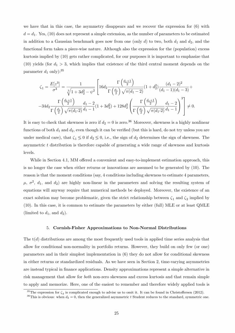
(10) yields (for 1 3, which implies that existence of the third central moment depends on the
parameter 1 only):35
1 =[3]
3=
1
3
q1 + 322 − 2
⎡⎣162 Γ³1+12
´Γ³12
´p(1 − 2)
(1 + 22)(1 − 2)2
(1 − 1)(1 − 3)+
−342Γ³1+12
´Γ³12
´p(1-2)
1 − 21 − 1(1 + 3
22) + 128
32
⎛⎝ Γ³1+12
´Γ³12
´p(1-2)
1 − 21 − 1
⎞⎠3⎤⎥⎦ 6= 0
It is easy to check that skewness is zero if 2 = 0 is zero.36 Moreover, skewness is a highly nonlinear
functions of both 1 and 2, even though it can be verified (but this is hard, do not try unless you are
under medical care), that 1 ≶ 0 if 2 ≶ 0 i.e., the sign of 2 determines the sign of skewness. Theasymmetric distribution is therefore capable of generating a wide range of skewness and kurtosis
levels.
While in Section 4.1, MM offered a convenient and easy-to-implement estimation approach, this
is no longer the case when either returns or innovations are assumed to be generated by (10). The
reason is that the moment conditions (say, 4 conditions including skewness to estimate 4 parameters,
, 2, 1, and 2) are highly non-linear in the parameters and solving the resulting system of
equations will anyway require that numerical methods be deployed. Moreover, the existence of an
exact solution may become problematic, given the strict relationship between 1 and 2 implied by
(10). In this case, it is common to estimate the parameters by either (full) MLE or at least QMLE
(limited to 1, and 2).
5. Cornish-Fisher Approximations to Non-Normal Distributions
The t() distributions are among the most frequently used tools in applied time series analysis that
allow for conditional non-normality in portfolio returns. However, they build on only few (or one)
parameters and in their simplest implementation in (6) they do not allow for conditional skewness
in either returns or standardized residuals. As we have seen in Section 2, time-varying asymmetries
are instead typical in finance applications. Density approximations represent a simple alternative in
risk management that allow for both non-zero skewness and excess kurtosis and that remain simple
to apply and memorize. Here, one of the easiest to remember and therefore widely applied tools is
35The expression for 2 is complicated enough to advise us to omit it. It can be found in Christoffersen (2012).36This is obvious: when 2 = 0 then the generalized asymmetric Student reduces to the standard, symmetric one.
25

represented by Cornish-Fisher approximations (see Jaschke, 2002):37
+1() = −−1 +1 − +1
−1 ≡ Φ−1 +16
£(Φ−1 )
2 − 1¤+ 224
£(Φ−1 )
3 − 3Φ−1¤− 21
36
£2(Φ−1 )
3 − 5Φ−1¤
where Φ−1 ≡ Φ−1() to save space and 1, 2 are population skewness and excess kurtosis, respec-
tively. The Cornish-Fisher quantile, −1 , can be viewed as a Taylor expansion around a normal,
baseline distribution. This can be easily seen from the fact that if we have neither skewness nor
excess kurtosis so that 1 = 2 = 0, then we simply get the quantile of the normal distribution back,
−1 = Φ−1 , and +1() = +1().
For instance, for our monthly data set on U.S. stock portfolio returns, +1 = 089%, +1 =
466%, 1 = −0584, and 2 = 2226. Because Φ−1 = −2326, we have:
16
£(Φ−1 )
2 − 1¤ = −0423 224
£(Φ−1 )
3 − 3Φ−1¤= −0520 − 21
36
£2(Φ−1 )
3 − 5Φ−1¤= 0128
Therefore −1001 = −3148 and [
+1(1%) = 1377% per month. You can use the difference
between [
+1(1%) = 1377% and [
+1(1%) = 1095% to quantify the importance of negative
skewness for monthly risk management (2.82% per month).38 Figure 8 plots 1% VaR for monthly
US stock returns data (i.e., again +1 = 089%, +1 = 466%) when one changes sample estimates
of skewness (1) and excess kurtosis (2), keeping in mind that 2 −3.
Figure 8: 1% Value-at-Risk estimates as a function of skewness and excess kurtosis
The dot tries to represent in the three-dimensional space the Gaussian benchmark. On the one hand,
Figure 8 shows that is easy for a CF VaR to exceed the normal estimate. In particular, this occurs
37This way of presenting CF approximations takes as a given that many other types of approximations exist in the
statistics literature. For instance, the Gram-Charlier’s approach to return distribution modeling is rather popular in
option pricing. However, CF approximations are often viewed as the basis for an approximation to the value-at-risk
from a wide range of conditionally non-normal distributions.
38Needless to say, our earlier Gaussian VaR estimate of [ +1(1%) = 994% looks increasingly dangerous, as in a
single day it may come to under-estimate the VaR of the U.S. index by a stunning 400 basis points!
26

for all combinations of negative sample skewness and non-negative excess kurtosis. On the other
hand, and this is rather interesting as many risk managers normally think that accommodating for
departures from normality will always increase capital charges, Figure 8 also shows the existence of
combinations that yield estimates of VaR that are below the Gaussian estimate. In particular, this
occurs when skewness is positive and rather large and for small or negative excess kurtosis, which
is of course what we would expect.
5.1. A numerical example
Consider the main statistical features of the daily time series of S&P 500 index returns over the
sample period 1926-2009. These are characterized by a daily mean of 0.0413% and a daily standard
deviation of 1.1521%. Their skewness is -0.00074 and their excess kurtosis is 17.1563. Figure 9
computes the 5% VaR exploiting the CF approximation on a grid of values for daily skewness built
as [-2 -1.9 -1.8 ... 1.8 1.9 2] and on a grid of values for excess kurtosis built as [-2.8 -2.6 -2.4 ... 17.6
17.8 18].
‐2
‐1.1
‐0.2
0.7
1.6
0.00.30.60.91.21.51.82.12.42.7
3.0
‐3‐10134678101113141517
Cornish Fisher Approximations for VaR 5%
Figure 9: 5% Value-at-Risk estimates as a function of skewness and excess kurtosis
Let’s now calculate a standard Gaussian 5% VaR assessment for S&P 500 daily returns: this can
be derived from the two-dimensional Cornish-Fisher approximation setting skewness to 0 and ex-
cess kurtosis to 0: VaR005 = 185% This implies that a standard Gaussian 5% VaR will over -
estimate the VaR005: because S&P500 skewness is -0.00074 and excess kurtosis is 17.1563, your
two-dimensional array should reveal an approximate VaR005 of 1.46%. Two comments are in order.
First, the mistake is obvious but not as bad as you may have expected (the difference is 0.39%
which even at a daily frequency may seem moderate). Second, to your shock the mistake does not
have the sign you expect: this depends on the fact that while in the lectures, the 1% VaR surface
is steeply monotonic increasing in excess kurtosis, for a 5% VaR surface, the shape is (weakly)
monotone decreasing. Why this may be, it is easy to see, as the term
224[(Φ−1005)
3 − 3Φ−1005] ' 0484224
0
27

Because +1() = −500−1005, i.e., the Cornish-Fisher percentile is multiplied by a −1
coefficient, a positive224[(Φ−1005)
3 − 3Φ−1005] term means that the higher excess kurtosis is, the lower
the VaR005 is. Now, the daily S&P 500 data present an enormous excess kurtosis of 17.2. This
lowers VaR005 below the Gaussian VaR005 benchmark of 1.85%. Finally,
+1(005) = −500[(− 2)]12−1 ()
= −11521[235435]12(−20835) = 1764%
where comes from the method of moment estimation equation
= 4 +6
[()− 3= 4 +
6
20156− 3 = 435
Notice that also the t-Student estimate of VaR005 (1.76%) is lower than the Gaussian VaR estimate,
although the two are in this case rather close.
If you repeat this exercise for the case of = 01% you get Figure 10:
‐2
‐1.1
‐0.2
0.7
1.6
‐8.0
‐3.0
2.0
7.0
12.0
17.0
‐2.8
‐1
0.8
2.6
4.4
6.28
9.8
11.6
13.4
15.2
17
Cornish Fisher Approximations for VaR 0.1%
Figure 10: 0.1% Value-at-Risk estimates as a function of skewness and excess kurtosis
Let’s now calculate a standard Gaussian 0.1% VaR assessment for S&P 500 daily returns: this can
be derived from the two-dimensional Cornish-Fisher approximation setting skewness to 0 and excess
kurtosis to 0: VaR0001 = 352% This implies that a standard Gaussian 5% VaR will severely under -
estimate the VaR001: because S&P500 skewness is -0.00074 and excess kurtosis is 17.1563, your
two-dimensional array should reveal an approximate VaR005 of 20.50%. Both the three-dimensional
plot and the comparison between the CF and the Gaussian VaR0001 conform with your expectations.
First, a Gaussian VaR0001 gives a massive underestimation of the S&P 500 VaR0001 which is as
large as 20.5% as a result of a huge excess kurtosis. Second, in the diagram, the CF VaR0001
increases in excess kurtosis and decreases in skewness. In the case of excess kurtosis, this occurs
because the term224[(Φ−10001)
3 − 3Φ−10001] ' −2024224
0
which implies that the higher excess kurtosis is, the higher is VaR0001. Now, the daily S&P 500
data present an enormous excess kurtosis of 17.2. This increases VaR0001 well above the Gaussian
28

VaR0001 benchmark of 3.67%. Finally,
+1(0001) = −500[(− 2)]12−1 ()
= −11521[235435]12(−6618) = 5604%
where = 465. Even though such estimate certainly exceeds the 3.52% obtained under a Gaussian
benchmark, this +1(0001) pales when compared to the 20.50% full CF VaR.
Finally, some useful insight may be derived from fixing the first four moments of S&P 500
daily returns to be: mean of 0.0413%, standard deviation of 1.1521%, skewness of -0.00074, excess
kurtosis of 17.1563. Figure 11 plots the VaR() measure as a function of ranging on the grid
[0.05% 0.1% 0.15%... 4.9% 4.95% 5%] for four statistical models: (i) a standard Gaussian VaR;
(ii) a Cornish-Fisher VaR with CF expansion arrested to the second order, i.e.,
2 = −
∙Φ−1 +
16
¡Φ−1
¢2 − 16
¸;
(iii) a standard four-moment Cornish-Fisher VaR as presented above; (iv) a t-Student VaR.
0
5
10
15
20
25
0 0.5 1 1.5 2 2.5 3 3.5 4 4.5 5
VaRp Under Different Models as a Function of p
Gaussian VaR Second‐order CF Cornish‐Fisher Approximation t Student VaR
Figure 11: VaR for different coverage probabilities and alternative econometric models
For high , there are only small differences among different VaR measures, and a Gaussian VaR may
even be higher than VaRs computed under different models. For low values of the Cornish-Fisher
VaR largely exceeds any other measure because of the large excess kurtosis of daily S&P 500 data.
Finally, as one should expect, S&P 500 returns have a skewness that is so small, that the differences
between Gaussian VaR and Cornish-Fisher VaR measures computed from a second-order Taylor
expansion (i.e., that reflects only skewness) are almost impossible to detect in the plot (if you pay
attention, we plotted four curves, but you can detect only three of them).
It is also possible to use the results in Figure 11 to propose one measure of the contribution of
skewness to the calculation of VaR and two measures of the contribution of excess kurtosis to the
calculation of VaR. This is what Figure 12 does. Note that different types of contributions are
29

measured on different axis/scales, to make the plot readable.
0.0000
0.0002
0.0004
0.0006
0.0008
0.0010
0.0012
0.0014
0.0016
‐2
2
6
10
14
18
22
0 0.5 1 1.5 2 2.5 3 3.5 4 4.5 5
Contribution of Skewness and Kurtosis to VaRp
Contribution of Kurtosis ‐ measure 1 Contribution of Kurtosis ‐ measure 2Contribution of Skewness
Figure 12: Measures of contributions of skewness and excess kurtosis to VaR
The measure of skewness is obvious, the difference between the second-order CF VaR and the
Gaussian VaR measure. On the opposite, for kurtosis we have two possible measures: the difference
between the standard CF VaR and the Gaussian VaR, net of the effect of skewness (as determined
above); the difference between the symmetric t-Student VaR and the Gaussian VaR, because in the
case of t-Student, any asymmetries cannot be captured. Figure 12 shows such measures, with the
skewness contribution plotted on the right axis. Clearly, the contribution of skewness is very small,
because S&P 500 returns present very modest asymmetries. The contribution of kurtosis is instead
massive, especially when measured using CF VaR measures.
6. Direct Estimation of Tail Risk: A Quick Introduction to Extreme Value Theory
The approach to risk management followed so far was a bit odd: we are keen to model and obtain
accurate estimates of the left tail of the density of portfolio returns; however, to accomplish this
goal, we have used time series methods to (mostly, parametrically) model the time-variation in the
entire density of returns. For instance, if you care for getting a precise estimate of [ +1(1%) and
use a -Student GARCH(1,1) model (see Terasvirta, 2009),
&+1 = (
q + (&
)2 + 2 )+1 +1 ∼ IID ()
you are clearly modelling the dynamics–as driven by changes in 2 induced by the GARCH–over
the entire density over time. But given that your interest is in [ +1(1%) one wonders when and
how it can be optimal for you to deal with all the data in the sample and their distribution. Can
we do any differently? This is what extreme value theory (EVT) accomplishes for you (see McNeil,
1998).
Typically, the biggest risks to a portfolio are represented by the unexpected occurrence of a
single large negative return. Having an as-precise-as-possible knowledge of the probabilities of
such extremes is therefore essential. One assumption typically employed by EVT greatly simplifies
30

this task: an appropriately scaled version of asset returns–for instance, standardized returns from
some GARCH model–must be IID according to some distribution, it is not important the exact
parametric nature of such a distribution:39
+1 =+1
+1IID D(0 1)
Although early on this will appear to be odd, EVT studies the probability that, conditioning that
they exceed a threshold , the standardized returns less a threshold are below a value :
() ≡ Pr{ − ≤ | } (11)
where 0. Admittedly, the probabilistic object in (11) has no straightforward meaning and it
does trigger the question: why should a risk or portfolio manager care for computing and reporting
it? Figure 13 represents (11) and clarifies that this represents the probability of a “slice” of the
support for . Figure 13 marks a progress in our understanding for the fascination of EVT experts
for (11). However, in Figure 13, what remains odd is that we apparently care for a probability slice
from the right tail of the distribution of standardized returns.
u
x+u
‐
Figure 13: Graphical representation of () ≡Pr { − ≤ | }
Yet, if you instead of conditioning on some positive value of you condition on −, the negativeof a given standardized return, then, given 0,
1− () ≡ 1− Pr{− − ≤ |− }= 1− Pr{− ≤ + | −}= 1− Pr{ −(+ )| −}= Pr{ ≤ −(+ )| −}
where we have repeatedly exploited the fact that if − then −1 · (−) −1 · or − andthat that 1− Pr{ |} = Pr{ ≤ |}. At this point, the finding that
() = 1− Pr{ ≤ −(+ )| −}39Unfortunately, the IID assumption is usually inappropriate at short horizons due to the time-varying variance
patterns of high-frequency returns. We therefore need to get rid of the variance dynamics before applying EVT, which
is what we have assumed above.
31

is of extreme interest: () represents the complement to 1 of Pr{ ≤ −( + )| −} whichis the probability that the standardized return does not exceed a negative value −( + ) 0
conditioning on the fact that such a standardized return is below a threshold − 0 For instance, if
you set = 0 and to be some large positive value, 1−() equals the probability that standardizedportfolio returns are below − conditioning on the fact that these returns are negative and hencein the left tail: this quantity is clearly relevant to all portfolio and risk managers. Interestingly
then, while is the analog to defining the tail of interest through a point in the empirical support
of , acts as a truncation parameter: it defines how far in the (left) tail our modelling effort ought
to go.
In practice, how do we compute ()? On the one hand, this is all we have been doing in
this set of lecture notes: any (parametric or even non-parametric) time series model will lead to an
estimate of the PDF and hence (say, by simple numerical integration) to an estimate of the CDF
(; θ) from which (; θ) can always be computed as
() =Pr{ ≤ + }
Pr{ } = (+ )− ()
1− () (12)
that derives from the fact that for two generic events and ,
(|) = ( ∩) ()
() 0
and the fact that over the real line, Pr{ } = ()− (). In principle, as many of our modelshave implied, such an estimate of the CDF may even be a conditional one, i.e., +1(; θ|F).However, as we have commented already, this seems rather counter-intuitive: if we just need an
estimate of +1(; θ|F), it seems a waste of energies and computational power to first estimate the
entire conditional CDF, +1(; θ|F) to then compute +1(; θ|F) which may be of interest to
a risk manager. In fact, EVT relies one very interesting–once more, almost “magical”–statistical
result: if the series is independently and identically distributed over time (IID), as you let the
threshold, , get large (→∞ so that one is looking at the extreme tail of the CDF), almost any
CDF distribution, (), for observations beyond the threshold converges to the generalized Pareto
(GP) distribution, (; ), where 0 and40
()→ (; ) =
⎧⎨⎩ 1−³1 +
´− 1if 6= 0
1− exp³−
´if = 0
where
( ≥ if ≥ 0 ≤ ≤ −
if 0
is the key parameter of the GPD. It is also called the tail-index parameter and it controls the
shape of the distribution tail and in particular how quickly the tail goes to zero when the extreme,
, goes to infinity. 0 implies a thick-tailed distribution such as the -Student; = 0 leads
to a Gaussian density; 0 to a thin-tailed distribution. The fact that for = 0 one obtains
a Gaussian distribution should be no surprise: when tails decay exponentially, the advantages of
using a negative power function (see our discussion in Section 4) disappear.
40Read carefully: (; ) approximates the truncated CDF beyond the threshold as →∞.
32

At this point, even though for any CDF we have that () → (; ) it remains the fact
that the expression in (12) is unwieldy to use in practice. Therefore, let’s re-write it instead as (for
≡ + a change of variable that helps in what follows):
( − ) = ()− ()
1− ()=⇒ [1− ()]( − ) = ()− ()
=⇒ () = () + [1− ()]( − ) = 1− 1 + () + [1− ()]( − )
= 1− [1− ()] + [1− ()]( − ) = 1− [1− ()][1− ( − )]
Now let denote the total sample size and let denote the number of observations beyond the
threshold, : ≡P
=1 ( ). The term 1 − () can then be estimated simply by the
proportion of data points beyond the threshold, , call it
1− () =
( − ) can be estimated by MLE on the standardized observations in excess of the chosen
threshold . In practice, assuming 6= 0, suppose we have somehow obtained ML estimates of
and in
(; ) =
⎧⎨⎩ 1−³1 +
´− 1if 6= 0
1− exp³−
´if = 0
which we know to hold as →∞. Then the resulting ML estimator of the CDF () is:
() = 1−
[1− ( − )] = 1−
⎡⎣1− 1 +Ã1 +
!− 1
⎤⎦ = 1−
⎡⎣Ã1 +
!− 1
⎤⎦so that
lim→∞ () =
1−
∙³1 +
´− 1
¸− 1 +
= 1−⎡⎣Ã1 +
!− 1
⎤⎦ This way of proceeding represents the “high” way because it is based on MLE plus an application
of the GPD approximation result for IID series (see e.g., Huisman, Koedijk, Kool, and Palm, 2001).
However, in the practice of applications of EVT to risk management, this is not the most common
approach: when 0 (the case of fat tails is obviously the most common in finance, as we have
seen in Sections 2 and 3 of this chapter), then a very easy-to-compute estimator exists, namely
Hill’s estimator. The idea is that a rather complex ML estimation that exploits the asymptotic
GPD result may be approximated in the following way (for ):
Pr{ } = 1− () = ()− 1 ≈
− 1
where () is an appropriately chosen, slowly varying function of that works for most distributions
and is thus (because it is approximately constant as a function of ) set to a constant, .41 Of course,
41Formally, this can be obtained by developing in a Taylor expansion ()−1 and absorbing the parameter
into the constant (which will non-linearly depend on ).
33

in practice, both the constant and the parameter will have to be estimated. We start by writing
the log-likelihood function for the approximate conditional density for all observations as:
( ) =Q=1
(| ) =Q=1
()
1− ()= −
Q=1
1
− 1−1
1
− 1
The expression ()1 − () in the product involving only observations to the right of the
threshold derives from the fact that
(| ) =()
Pr( )=
()
1− ()
for . Moreover,
() = ()
=
∙1−
−1
¸
=1
− 1−1
Therefore the log-likelihood function is
L( ) = log( ) = −P=1
½− log − (1
+ 1) log +
1
log
¾
Taking first-order conditions and solving, delivers a simple estimator for :42
=1
X=1
ln³
´
which is easy to implement and remember. At this point, we can also estimate the parameter
by ensuring that the fraction of observations beyond the threshold is accurately captured by the
density as in () = 1− :
1− − 1
= 1− =⇒ =
1
from the fact that we have approximated () as 1 − −1. At this point, collecting all these
approximation/estimation results we have that
() = 1− − 1
= 1−
1
− 1
= 1−
³
´− 1
= 1−
³
´− 1
=1 ln(
)−1
where the first line follows from () ≈ 1 − − 1 and the remaining steps have simply plugged
estimates in the original equations. Because we had defined ≡ + equivalently we have:
(+ ) = 1−
³1 +
´− 1
=1 ln(1+
)−1
which is a Hill/ETV estimator of the CDF when →∞ i.e., of the extreme right tail of distribution
of (the negative of) standardized returns. This seems rather messy, but the pay-off has been quite
42In practice, the Hill’s estimator
is an approximate MLE in the sense that it is derived from taking an approx-
imation of the conditional PDF under the EVT (as → ∞) and developing and solving FOCs of the correspondingapproximate log-likelihood function.
34

formidable: we now have a closed-form expression for the shape of the very far CDF of portfolio
percentage losses which does not require numerical optimization within ML estimation. Such an
estimate is therefore easy to calculate and to apply within (12), knowing that if ( + ) is
available, then
() =
(+ )− ()
1− ()
Obviously, and by construction, such an approximation is increasingly good as →∞.How do you know whether and how your EVT (Hill’s) estimator is fitting the data well enough?
Typically, portfolio and risk managers use our traditional tool to judge of this achievement, i.e., a
(partial) QQ plots. A partial QQ plot consists of a standard QQ plot derived and presented only
for (standardized) returns below some threshold loss − 0 It can be shown that the partial QQ
plot from EVT can be built representing in a classical Cartesian diagram the relationship
{ } =(
∙− 05
·
¸−
)
where is the th standardized loss sorted in descending order (i.e., for negative standardized
returns ). The first and basic logical step consists in taking a time series of portfolio returns and
analyzing their (standardized) opposite, i.e., ≡ −. This way, one formally looks at the
right-tail conditioning on some threshold 0 even though the standard logical VaR meanings
obtain. In a statistical perspective, the first and initial step is to set the estimated cumulative
probability function equal to 1 − so that there is only a probability of getting a standardized
loss worse than the quantile, (−11−), which is implicitly defined by (−11−) = 1− or
1−
Ã−11−
!−1= 1− =⇒ −11−
=
∙
¸−=⇒ −11− =
∙
¸−
At this point, the Q-Q plot can be constructed as follows: First, sort all standardized returns, ,
in ascending order, and call the th sorted value . Second, calculate the empirical probability
of getting a value below the actual as (− 5) , where is the total number of observations.43 Wecan then scatter plot the standardized and sorted returns on the Y-axis against the implied ETV
quantiles on the X-axis as follows:
{ } =
⎧⎪⎪⎪⎨⎪⎪⎪⎩
⎡⎢⎢⎣ (− 05)| {z }
matching s quantile
⎤⎥⎥⎦−
⎫⎪⎪⎪⎬⎪⎪⎪⎭
If the data were distributed according to the assumed EVT distribution for , then the scatter
plot should conform roughly to the the 45-degree line.
Because they are representations of partial CDF estimators–limited to the right tail of negative
standardized returns, that is the left tail of actual standardized portfolio returns–ETV-based QQ
43The subtraction of .5 is an adjustment allowing for a continuous distribution.
35

plots are frequently excellent, which fully reflects the power of EVT methods to capture in extremely
accurate ways the features of the (extreme) tails of the financial data, see the example in Figure
14. Clearly, everything works in Figure 14, as shown by the fact that all the percentiles practically
fall on the left-most branch of the 45-degree line. However, not all is as good as it seems: as we
shall see in the worked-out MatlabR°session at the end of this chapter, these EVT-induced partial
QQ plots obviously suffer from consistency issues, as the same quantile may strongly vary with the
threshold . In fact, and with reference to the same identical quantiles, if one changes , plots that
are very different (i.e., much less comforting) than Figure 14 might be obtained and this is logically
problematic, as it means that the same method and estimator (Hill’s approximate MLE) may give
different results as a function of the nuisance parameter represented by .
– u
Figure 14: Partial QQ plot for an EVT tail model of () ≡Pr { − ≤ | }
In itself, the choice of appears problematic because a researcher must balance a delicate trade-
off between bias and variance. If is set too large, then only very few observations are left in
the tail and the estimate of the tail parameter, , will be very uncertain because it is based on
a small sample. If on the other hand is set to be too small, then the EVT key result that all
CDFs may be approximated by a GPD may fail, simply because this result held as → ∞ ; thismeans that the data to the right of the threshold do not conform sufficiently well to the generalized
Pareto distribution to generate unbiased estimates of . For samples of around 1,000 observations,
corresponding to about 5 years of daily data, a good rule of thumb (as shown by a number of
simulation studies) is to set the threshold so as to keep the largest 5% of the observations for
estimating –that is, we set = 50. The threshold will then simply be the 95th percentile of
the data.
In a similar fashion, Hill’s -percent VaR can be computed as (in the simple case of the one-step
ahead VaR estimate):
+1 (;) = −11−+1 +
+1 =
∙
¸−+1 +
+1
where +1 = −+1 represents the conditional mean not for returns but for the negative of returns,
36

≡ −.44 The reason for using the (1− )th quantile from the EVT loss distribution in the VaR
with coverage rate is that the quantile such that (1 − ) × 100% of losses are smaller than it is
the same as minus the quantile such that × 100% of returns are smaller than it. Note that the
VaR expression remains conditional on the threshold ; this an additional parameter that tells the
algorithm how specific (tailored) to the tail you want your VaR estimate to be. However, as already
commented above with reference to the partial QQ plots, this may be a source of problems: for
instance one may find that +1 (1%; 2%) = 456% but
+1 (1%; 3%) = 504%: even though
they are both sensible (as +1 which is a minimal consistency requirement), which one
should we pick to calculate portfolio and risk management capital requirements?
In the practice of risk management, it is well known that normal and EVT distributions often
lead to similar 1% VaRs but to very different 0.1% VaRs due to the different tail shapes that the
two methods imply, i.e., the fact that Gaussian models often lead to excessively thin estimates of
the left tail. Figure 15 represents one such case: even though the 1% VaR under normal and EVT
tail estimates are identical, the left tail behavior is sufficiently different to potentially cause VaR
estimates obtained for 1% to differ considerably. The tail of the normal distribution very
quickly converges to zero, whereas the EVT distribution has a long and fat tail.
EVT based on = 0.5
Very different tail behavior
Figure 15: Different tail behavior of normal vs. EVT distribution models
Visually, this is due to the existence of a crossing point in the far left tail of the two different
distributions. Therefore standard Basel-style VaR calculations based on a 1% coverage rate may
conceal the fact that the tail shape of the distribution does not conform to the normal distribution:
in Figure 15, VaRs below 1% will differ by a factor as large as 1 million! In this example, the portfolio
with the EVT distribution is much riskier than the portfolio with the normal distribution in that
it implies non-negligible probabilities of very large losses. What can we do about it? The answer is
to supplement VaR measures with other measures such as plots in which VaR is represented as a
function of (i.e., one goes from seeing VaR as an estimate of an unknown parameter to consider
VaR as an estimate of a function of , to assess the behavior of the tails) or to switch to alternative
44The use of the negative of returns explains the absence of negative signs in the expression.
37

risk management criteria, for instance the Expected Shortfall (also called TailVaR), see Appendix
A for a quick review of the concept.
How can you compute ES in practice? For the remainder of this Section, assume +1 = 0%
Let’s start with the bad news: it is more complex than in the case of the plain-vanilla VaR because
ES actually conditions on VaR. In fact, usually one has to perform simulations under the null of
a given econometric model to be able to compute an estimate of ES. Now it is time for the good
news: at least in the Gaussian case, one can find a (sort of) closed form expression:
+1() = −[+1|
+1 − +1()] = +1
³− +1()
+1
´Φ³− +1()
+1
´ = +1¡Φ−1
¢
where the last equality follows from +1() = −+1Φ−1 and Φ¡−Φ−1 ¢ = Here (·) denotes
the standard normal PDF, while Φ (·) is, as before, the standard normal CDF. For instance, if+1 = 12%, +1() = 0012{[(−2)−12 exp(−(−233)22)]001} = 317% from
() = (−2)−12 expµ−
2
2
Interestingly, the ratio between +1() and +1() possesses two key properties. First, under
Gaussian portfolio returns, as → 0+, +1() +1() → 1 and so there is little difference
between the two measures. This makes intuitive sense: the ES for a very extreme value of basically
reduces to the VaR estimate itself as there is very little probability mass left to the left of VaR. In
general, however, the ratio of ES to VaR for fat-tailed distribution will be higher than 1, which was
already the intuitive point of Figure 15 above. Second, for EVT distributions, when goes to zero,
the ES to VaR ratio converges to
lim→0+
+1()
+1()=
1
1−
so that as → 1 (which is revealing of fat tails, as claimed above), +1() +1()→ +∞.45Moreover, the larger (closer to 1) is 1 the larger is +1() for given +1().
Appendix A – Basic Value-at-Risk Formulas
Let’s review the definition of relative value-at-risk (VaR): VaR simply answers the question
“What percentage loss on a given portfolio is such that it will only be exceeded × 100% of
the time in the next trading periods (say, days)?” Formally:
0 is such that Pr( − ) =
45For instance, in Figure 15, where = 05, the ES to VaR ratio is roughly 2, even though the 1% VaR is the same
in the two distributions. Thus, the ES measure is more revealing than the VaR about the magnitude of losses larger
than the VaR.
38

where is a continuously compounded portfolio return between time and + , i.e.,
≡ ln
+ − ln , where
is the portfolio value. The absolute $ has a similar
definition with “dollar/euro (or your favorite currency)” replacing “percentage” in the definition
above:
$ 0 is such that Pr(exp[ ] exp[− ]) =
or by subtracting 1 from both sides inside the probability definitions and multiplying by ,
Pr([ +
]− 1 exp[− ]− 1) = Pr(
+ − (exp[− ]− 1)
)
= Pr(−( + −
) −(exp[− ]− 1) )
= Pr($ $ ) =
where $ ≡ (1− exp[− ]) .
It is well known that even though it is widely reported and discussed, the key shortcoming of VaR
is that it is concerned only with the range of the outcomes that exceed the VaR measure and not with
the overall magnitude (for instance, as captured by an expectation) of these losses. This magnitude,
however, should be of serious concern to a risk manager: large VaR exceedances–outcomes below
the VaR threshold–are much more likely to cause financial distress, such as bankruptcy, than
are small exceedances, and we therefore want to entertain a risk measure that accounts for the
magnitude of large losses as well as their probability.46 The challenge is to come up with a portfolio
risk measure that retains the simplicity of the VaR but conveys information regarding the shape of
the tail. Expected shortfall (ES), or TailVaR as it is sometimes called, does exactly this.47 Expected
shortfall (ES) is the expected value of tomorrow’s return, conditional on it being worse than the
VaR at given size :
+1() = −[+1|
+1 − +1()]
In essence, ES is just (the opposite of) a truncated conditional mean of portfolio returns, where the
truncation is provided by VaR. In particular, the negative signs in front of the expectation and the
VaR are needed because ES and VaR are defined as positive numbers.
Appendix B – A MatlabR°Workout
46Needless to say, the most complete measure of the probability and size of potential losses is the entire shape of
the tail of the distribution of losses beyond the VaR. Reporting the entire tail of the return distribution corresponds
to reporting VaRs for many different coverage rates, say ranging from .001% to 1% in increments of .001%. It may,
however, be less effective as a reporting tool to senior management than is a single VaR number, because visualizing
and discussing a function is always more complex than a single number that answers a rather simple question such as
“What’s the loss so that only 1% of potential losses will be worse over the relevant horizon?”47Additionally, Artzner et al. (1999) define the concept of a coherent risk measure and show that expected shortfall
(ES) is coherent whereas VaR is not.
39
Suppose you are a European investor and your reference currency is the Euro. You evaluate
the properties and risk of your equally weighted portfolio on a daily basis. Using daily data in
STOCKINT2013.XLS, construct daily returns (in Euros) using the three price indicesDS Market-
PRICE Indexes for three national stock markets, Germany, the US, and the UK.
1. For the sample period of 03/01/2000- 31/12/2011, plot the returns on each of the three
individual indices and for the equally weighted portfolio denominated in Euros. Just to make
sure you have correctly applied the exchange rate transformations, also proceed to plot the
exchange rates derived from your data set.
2. Assess the normality of your portfolio returns by computing and charting a QQ plot, a
Gaussian Kernel density estimator of the empirical distribution of data, and by performing
a Jarque-Bera test using daily portfolio data for the sample period 03/01/2000- 31/12/2011.
Perform these exercises both with reference to the raw portfolio returns (in euros) and with
reference to portfolio returns standardized using the unconditional sample mean standard de-
viation over your sample. In the case of the QQ plots, observe any differences between the plot
for raw vs. standardized returns and make sure to understand the source of any differences.
In the case of the Kernel density estimates, produce two plots, one comparing a Gaussian
density with the empirical kernel for portfolio returns and the other comparing a Gaussian
density with the empirical kernel for portfolio returns standardized using the unconditional
sample mean and standard deviation over your sample. In the case of the Jarque-Bera tests,
comment on the fact that the test results seem not to depend on whether raw or standard-
ized portfolio returns are employed. Are either the raw portfolio or the standardized returns
normally distributed?
3. Estimate a GARCH with leverage model over the same period and assess the normality of
the resulting standardized returns. You are free to shop among the asymmetric GARCH
models with Gaussian innovations that are offered by Matlab and the ones that have been
presented during the lectures. In any event make sure to verify that the estimates that you
have obtained are compatible with the stationarity of the variance process. Here it would be
useful if you were to estimate at least two different leverage GARCH models and compare the
normality of the resulting standardized residuals. Can you find any evidence that either of
the two volatility models induces standardized residuals that are consistent with the assumed
model, i.e., +1 = +1+1 with +1 IID (0 1)?
4. Simulate returns for your sample using at least one GARCH with leverage model, calibrated
on the basis of the estimation obtained under the previous point with normally distributed
residuals. Evaluate the normality properties of returns and standardized returns using QQ
plots and a Kernel density fit of the data.
40

5. Compute the 5% Value at Risk measure of the portfolio for each day of January 2012 (in the
Excel file, January 2012 has 20 days) using, respectively, a Normal quantile when variance is
constant (homoskedastic), a Normal quantile when conditional variance follows a GJR process,
a t-Sstudent quantile with the appropriately estimated number of degrees of freedom and a
Cornish-Fisher quantile and compare the results. Estimate the number of degrees of freedom
by maximum likelihood. In the case of a conditional t-Student density and of the Cornish-
Fisher approximation, use a conditional variance process calibrated on the filtered conditional
GJR variance in order to define standardized returns. The number of degrees of freedom for
the t-Student process should be estimated by QML.
6. Using QML, estimate a ()-NGARCH(1,1) model. Fix the variance parameters at their values
from question 3. If you have not estimated a (Gaussian) NGARCH(1,1) in question 3, it is
now time to estimate one. Set the starting value of equal to 10. Construct a QQ plot for
the standardized returns using the standardized () distribution under the QML estimate for
. Estimate again the ()-NGARCH(1,1) model using now full ML methods, i.e., estimating
jointly the t-Student parameter as well as the four parameters in the nonlinear GARCH
written as
2 = + (−1 − −1)2 + 2−1.
Is the resulting GARCH process stationary? Are the estimates of the coefficients different
across QML and ML methods and why? Construct a QQ plot for the standardized returns
using the standardized () distribution under the ML estimate for . Finally, plot and
compare the conditional volatilities resulting from your QML (two-step) and ML estimates of
the ()-NGARCH(1,1) model.
7. Estimate the EVTmodel on the standardized portfolio returns from a Gaussian NGARCH(1,1)
model using the Hill estimator. Use the 4% largest losses to estimate EVT. Calculate the 0.01%
standardized return quantile implied by each of the following models: Normal, (), Hill/EVT,
and Cornish-Fisher. Notice how different the 0.01% VaRs would be under these alternative
four models. Construct the QQ plot using the EVT distribution for the 4% largest losses.
Repeat the calculations and re-plot the QQ graph when the threshold is increased to be 8%.
Can you notice any differences? If so, why are these problematic?
8. Perform a simple asset allocation exercise under three alternative econometric specifications
using a Markowitz model, under a utility function of the type
( 2 ) = −
1
22 ,
with = 05, in order to determine optimal weights. Impose no short sale constraints on the
stock portfolios and no borrowing at the riskless rate. The alternative specifications are:
41

(a) Constant mean and a GARCH (1,1) model for conditional variance, assuming normally
distributed innovations.
(b) Constant mean and an EGARCH (1,1) model for conditional variance, assuming normally
distributed innovations.
(c) Constant mean and an EGARCH (1,1) model for conditional variance, assuming t-
Student distributed innovations.
Perform the estimation of the model parameters using a full sample of data until 02/01/2013.
Note that, just for simplicity (we shall relax this assumption later on) all models assume a
constant correlation among different asset classes, equal to sample estimate of their correla-
tions in pairs. Plot optimal weights and the resulting in-sample, realized Sharpe ratios of
your optimal portfolio under each of the three different frameworks. Comment the results.
[IMPORTANT: Use the toolboxes regression tool 1.m and mean variance multiperiod.m that
have been made available with this exercise set]
Solution
This solution is a commented version of the MATLAB code Ex CondDist VaRs 2013.m posted
on the course web site. Please make sure to use a “Save Path” to include jplv7 among the directories
that MatlabR°reads looking for usable functions. The loading of the data is performed by:
filename=uigetfile(‘*.txt’);
data=dlmread(filename);
The above two lines import only the numbers, not the strings, from a .txt file.48 The following
lines of the codes take care of the strings:
filename=uigetfile(‘*.txt’);
fid = fopen(filename);
labels = textscan(fid, ‘%s %s %s %s %s %s %s %s %s %s’);
fclose(fid);
1. The plot requires that the data are read in and transformed in euros using appropriate ex-
change rate log-changes, that need to be computed from the raw data, see the posted code for
details on these operations. The following lines proceed to convert Excel serial date numbers
into MATLAB serial date numbers (the function x2mdate(·)), set the dates to correspondto the beginning and the end of the sample, while the third and final dates are the beginning
and the end of the out-of-sample (OOS) period:
48The reason for loading from a .txt file in place of the usual Excel is to favor usage from Mac computers that
sometimes have issues with reading directly from Excel, because of copyright issues with shareware spreadsheets.
42

date=datenum(data(:,1));
date=x2mdate(date);
f=[‘02/01/2006’;‘31/12/2010’; ‘03/01/2013’];
date find=datenum(f,‘dd/mm/yyyy’);
ind=datefind(date find,date);
The figure is then produced using the a set of instructions that is not be commented in detail
because their structure closely resembles other plots proposed in Lab 1, see worked-out exercise in
chapter 4. Figure A1 shows the euro-denominated returns on each of the four indices.
Figure A1:Daily portfolio returns on four national stock market indices
Even though these plots are affected by the movements of the /$ and $/$ exchange rates, the
volatility bursts recorded in early 2002 (Enron and Worldcom scandal and insolvency), the Summer
of 2011 (European sovereign debt crisis), and especially the North-American phase of the great
financial crisis in 2008-2009 are well-visible.
Figure A2:Daily portfolio indices and exchange rates
43

As requested, Figure A2 plots the values of both indices and implied exchange rates, mostly to make
sure that the currency conversions have not introduced any anomalies.
2. The calculation of the unconditional sample standard deviation and the standardization of
portfolio returns is simply performed by the lines of code:
unc std=std(port ret(ind(1):ind(2)));
std portret=(port ret(ind(1):ind(2))-mean(port ret(ind(1):ind(2))))./unc std;
Note that standardizing by the unconditional standard deviation is equivalent to divide by a con-
stant, which is important in what follows. The set of instructions that produces QQ plots and
displays them horizontally to allow a comparison of the plots of raw vs. standardized returns
iterates on the simple function:
qqplot(RET(:,i));
where qqplot displays a quantile-quantile plot of the sample quantiles of X versus theoretical
quantiles from a normal distribution. If the distribution of X is normal, the plot will be close to
linear. The plot has the sample data displayed with the plot symbol ‘+’.49 Figure A3 displays the
two QQ plots and emphasizes the strong, obvious non-normality of both raw and standardized data.
Figure A3:Quantile-quantile plots for raw vs. standardized returns (under constant variance)
The kernel density fit comparisons occur between a normal distribution, that is simply repre-
sented by a simulation performed by the lines of codes
49Superimposed on the plot is a line joining the first and third quartiles of each distribution (this is a robust linear
fit of the order statistics of the two samples). This line is extrapolated out to the ends of the sample to help evaluate
the linearity of the data. Note that ‘qqplot(X,PD)’ would create instead an empirical quantile-quantile plot of the
quantiles of the data in the vector X versus the quantiles of the distribution specified by PD.
44

norm=randn(1000*rows(RET(:,1)),1);
norm1=mean(RET(:,1))+std(RET(:,1)).*norm;
norm2=mean(RET(:,2))+std(RET(:,2)).*norm;
[Fnorm1,XInorm1]=ksdensity(norm1,‘kernel’,‘normal’);
[Fnorm2,XInorm2]=ksdensity(norm2,‘kernel’,‘normal’);
To obtain a smooth Gaussian bell-shaped curve, you should generate a large number of values,
while the second and third lines ensure that the Gaussian random numbers will have the same
mean and variance as raw portfolio returns (however, by construction std(RET(:,2)) = 1). [f,xi]
= ksdensity(x) computes a probability density estimate of the sample in the vector x. f is the
vector of density values evaluated at the points in xi. The estimate is based on a normal kernel
function, using a window parameter (bandwidth) that is a function of the number of points in
x. The density is evaluated at 100 equally spaced points that cover the range of the data in x.
‘kernel’ specifies the type of kernel smoother to use. The possibilities are ‘normal’ (the default),
‘box’, ‘triangle’, ‘epanechnikov’. The following lines of codes perform the normal kernel density
estimation with reference to the actual data, both raw and standardized:
[F1,XI1]=ksdensity(RET(:,1),‘kernel’,‘normal’);
[F2,XI2]=ksdensity(RET(:,2),‘kernel’,‘normal’);
Figure A4 shows the results of this exercise. Clearly, both raw and standardized data deviate from
a Gaussian benchmark in the same ways commented early on: tails are fatter (especially the left
one); “bumps” in probability in the tails; less probability mass than the normal around ±115standard deviations from the normal, but a more peaked density around the mean.
Figure A4:Kernel density estimates: raw and standardized data vs. Normal kernel
Finally, formal Jarque-Bera tests are performed and displayed in Matlab using the following
lines of code:
45
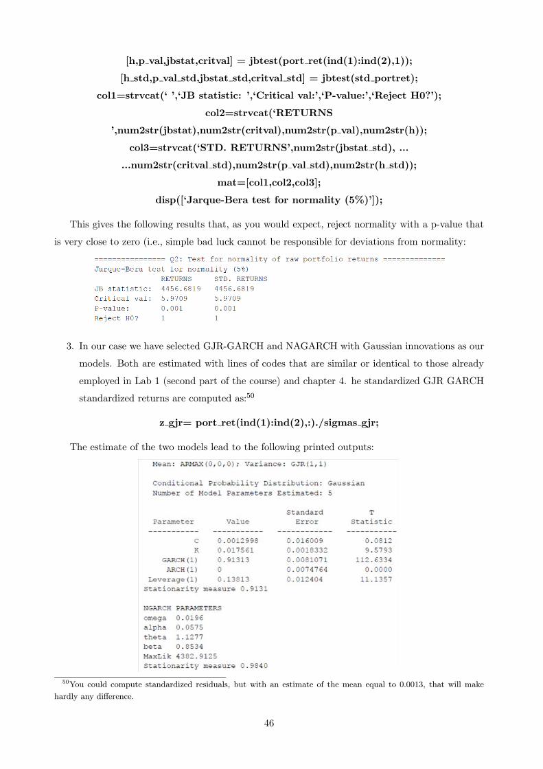
[h,p val,jbstat,critval] = jbtest(port ret(ind(1):ind(2),1));
[h std,p val std,jbstat std,critval std] = jbtest(std portret);
col1=strvcat(‘ ’,‘JB statistic: ’,‘Critical val:’,‘P-value:’,‘Reject H0?’);
col2=strvcat(‘RETURNS
’,num2str(jbstat),num2str(critval),num2str(p val),num2str(h));
col3=strvcat(‘STD. RETURNS’,num2str(jbstat std), ...
...num2str(critval std),num2str(p val std),num2str(h std));
mat=[col1,col2,col3];
disp([‘Jarque-Bera test for normality (5%)’]);
This gives the following results that, as you would expect, reject normality with a p-value that
is very close to zero (i.e., simple bad luck cannot be responsible for deviations from normality:
3. In our case we have selected GJR-GARCH and NAGARCH with Gaussian innovations as our
models. Both are estimated with lines of codes that are similar or identical to those already
employed in Lab 1 (second part of the course) and chapter 4. he standardized GJR GARCH
standardized returns are computed as:50
z gjr= port ret(ind(1):ind(2),:)./sigmas gjr;
The estimate of the two models lead to the following printed outputs:
50You could compute standardized residuals, but with an estimate of the mean equal to 0.0013, that will make
hardly any difference.
46

These give no surprises compared to the ones reported in chapter 4, for instance. Figure A5 compares
the standardized returns from the GJR and NAGARCH models. Clearly, there are differences, but
these seem to be modest at best.
Figure A5: Standardized returns from GJR(1,1) vs. NAGARCH(1,1)
In Figure A6, the QQ plots for both series of standardized returns are compared. While both
models seem to fit rather well the right tail of the data, as the standardized returns imply high-
order percentiles that are very similar to the normal ones, in the left tail–in fact this concerns
at least the first, left-most 25 percentiles of the distribution–the issues emphasized by Figure A3
remain. Also, there is no major difference between the two alternative asymmetric conditional
heteroskedastic models.
Figure A6: QQ plots for standardized returns of GJR vs. NAGARCH models
Figure A7 shows the same result using kernel density estimators. The improvement vs. Figure
47

A4 is obvious, but this does not seem to be sufficient yet.
Figure A7: Kernel density estimates of GJR vs. NAGARCH standardized returns
Finally, formal Jarque-Bera tests still lead to rejections of the null of normality of standardized
returns, with p-values that remain essentially nil.
4. The point of this question is for you to stop and visualize how “things should look like” if
you were to discover the true model that has generated the data. In this sense, the point
represents a sort of a break, I believe a useful one, in the flow of the exercise. The goal
is to show that if returns actually came from an assumed asymmetric GARCH model with
Gaussian innovations such as the ones estimated above, then the resulting (also simulated)
standardized returns would be normally distributed. Interestingly, Matlab provides a specific
garch-related function to perform simulations given the parameter estimates of a given model:
spec sim=garchset(‘Distribution’,‘Gaussian’,‘C’,0,‘VarianceModel’,‘GJR’,‘P’,param gjr.P,
...‘Q’,param gjr.Q,‘K’,param gjr.K,‘GARCH’,param gjr.GARCH,‘ARCH’,param gjr.ARCH,
...‘Leverage’,param gjr.Leverage);
[ret sim, sigma2 sim]=garchsim(spec sim,length(z ng),[]);
z sim=ret sim./sigma2 sim;
Using [Innovations,Sigmas,Series] = garchsim(Spec,NumSamples,NumPaths), each
simulated path is sampled at a length of NumSamples observations. The output consists of the
48

NumSamples × NumPaths matrix ‘Innovations’ (in which the rows are sequential observations, thecolumns are alternative paths), representing a mean zero, discrete-time stochastic process that fol-
lows the conditional variance specification defined in Spec. The simulations from the NAGARCH
model are obtained using:
zt=random(‘Normal’,0,1,length(z ng),1);
[r sim,s sim]=ngarch sim(param ng,var(port ret(ind(1):ind(2),:)),zt);
where ‘random’ is the general purpose random number generator in Matlab and ‘ngarch sim(par,sig2 0,innov)’
is our customized procedure that takes the NGARCH 4x1 parameter vector (omega; alpha; theta;
beta), initial variance (sig2 0), and a vector of innovations to generate a number ind(1)-ind(2) of
simulations. Figure A8 shows the QQ plots for both returns and standardized returns generated
from the GJR GARCH(1,1) model.
Figure A8: QQ Plots for raw and standardized GJR GARCH(1,1) simulated returns
The left-most plot concerns the raw returns and makes a point already discussed in chapter 4: if
the model is
+1 =³q
+ 2 + {0} + 2
´+1 +1 IID N (0 1)
then you know that even though +1 IID N (0 1) +1 will not be normally distributed, as shown
to the left of Figure A8. The righ-most plot concerns instead
+1 ≡ +1q + 2 + {0} + 2
IID N (0 1)
and shows that normality approximately obtains.51 Figure A9 makes the same point using not QQ
51Why only approximately? Think about it.
49

plots, but normal kernel density estimates.
Figure A9: Normal kernel density estimates applied to raw and standardized GJR simulated returns
Figures A10 and A11 repeat the experiment in Figures A8 and A9 with reference to simulated returns
and hence standardized returns from the other asymmetric model, a NAGARCH. The lesson they
teach is identical to Figures A8 and A9.
Figure A10: QQ Plots for raw and standardized NAGARCH(1,1) simulated returns
50
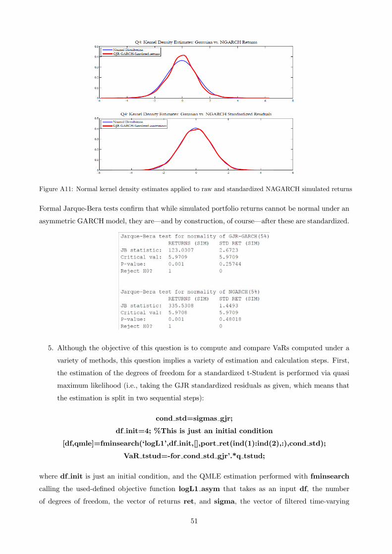
Figure A11: Normal kernel density estimates applied to raw and standardized NAGARCH simulated returns
Formal Jarque-Bera tests confirm that while simulated portfolio returns cannot be normal under an
asymmetric GARCH model, they are–and by construction, of course–after these are standardized.
5. Although the objective of this question is to compute and compare VaRs computed under a
variety of methods, this question implies a variety of estimation and calculation steps. First,
the estimation of the degrees of freedom for a standardized t-Student is performed via quasi
maximum likelihood (i.e., taking the GJR standardized residuals as given, which means that
the estimation is split in two sequential steps):
cond std=sigmas gjr;
df init=4; %This is just an initial condition
[df,qmle]=fminsearch(‘logL1’,df init,[],port ret(ind(1):ind(2),:),cond std);
VaR tstud=-for cond std gjr’.*q tstud;
where df init is just an initial condition, and the QMLE estimation performed with fminsearch
calling the used-defined objective function logL1 asym that takes as an input df, the number
of degrees of freedom, the vector of returns ret, and sigma, the vector of filtered time-varying
51
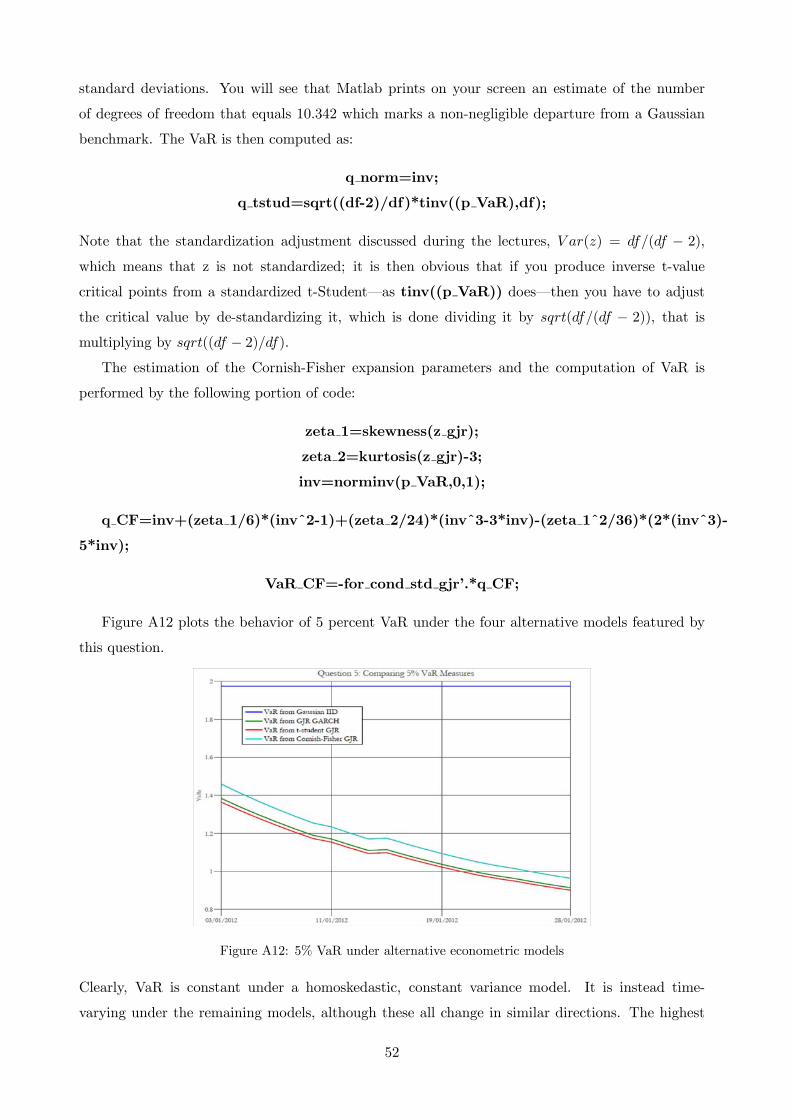
standard deviations. You will see that Matlab prints on your screen an estimate of the number
of degrees of freedom that equals 10.342 which marks a non-negligible departure from a Gaussian
benchmark. The VaR is then computed as:
q norm=inv;
q tstud=sqrt((df-2)/df)*tinv((p VaR),df);
Note that the standardization adjustment discussed during the lectures, () = ( − 2),which means that z is not standardized; it is then obvious that if you produce inverse t-value
critical points from a standardized t-Student–as tinv((p VaR)) does–then you have to adjust
the critical value by de-standardizing it, which is done dividing it by (( − 2)), that ismultiplying by (( − 2))
The estimation of the Cornish-Fisher expansion parameters and the computation of VaR is
performed by the following portion of code:
zeta 1=skewness(z gjr);
zeta 2=kurtosis(z gjr)-3;
inv=norminv(p VaR,0,1);
q CF=inv+(zeta 1/6)*(invˆ2-1)+(zeta 2/24)*(invˆ3-3*inv)-(zeta 1ˆ2/36)*(2*(invˆ3)-
5*inv);
VaR CF=-for cond std gjr’.*q CF;
Figure A12 plots the behavior of 5 percent VaR under the four alternative models featured by
this question.
Figure A12: 5% VaR under alternative econometric models
Clearly, VaR is constant under a homoskedastic, constant variance model. It is instead time-
varying under the remaining models, although these all change in similar directions. The highest
52

VaR estimates are yielded by the GJR GARCH(1,1) models, quite independently of the assumption
made on the distribution of the innovations (normal or t-Student). The small differences between
the normal and t-Student VaR estimates indicate that at a 5% level, the type of non-normalities that
a t-Student assumption may actually pick up remain limited, when the estimated number of degrees
of freedom is about 10.52 Finally, the VaR computed under a CF approximation is considerably
higher than the GJR GARCH VaR estimates: this is an indication of the presence of negative
skewness in portfolio returns that only a CF approximation may capture. Figure A12 emphasizes
once more the fact that adopting more complex, dynamic time series models is not always leading to
higher VaR estimates and more prudent risk management: in this example–also because volatility
has been declining during early 2012, after the Great Financial crisis and European sovereign debt
fears–constant variance models imply higher VaR estimates than richer models do.53
6. Starting from an initial condition df init=10, QML estimates of a NAGARCH with stan-
dardized t(d) innovations is performed by:
[df,qmle]=fminsearch(’logL1’,df init,[],port ret(ind(1):ind(2),:),sqrt(cond var ng));
where cond var ng is taken as given from question 3 above. The QML estimate of the number
of degrees of freedom is 10.342. The resulting QQ plot is shown in Figure A13: interestingly,
compared to Figure A6 where the NAGARCH innovations were normally distributed, marks a
strong improvement in the left tail, although the quality of the fit in the right tail appears inferior
to Figure A6.
Figure A13: QQ plot of QML estimate of t-Student NAGARCH(1,1) model
Interestingly, Figure A13 displays a QQ plot built from scratch and not using the Matlab function,
using the following code:
52This also derives from the fact that a 5 percent VaR is not really determined by the behavior of the density of
portfolio returns in the deep end of the left tail. Try and perform calculations afresh for a 1 percent VaR and you will
find interesting differences.53Of course, lower VaR, lower capital charges and capital requirements.
53

z ngarch=sort(z ng);
z=sort(port ret(ind(1)-1:ind(2)-1,:));
[R,C]=size(z);
rank=(1:R)’;
n=length(z);
quant tstud=tinv(((rank-0.5)/n),df);
cond var qmle=cond var ng;
qqplot(sqrt((df-2)/df)*quant tstud,z ngarch);
set(gcf,‘color’,‘w’);
title(‘Question 6: QQ Plot of NGARCH Standardized Residuals vs. Standardized
t(d) Distribution (QML Method)’,‘fontname’,‘garamond’,‘fontsize’,15);
The full ML estimation is performed in ways similar to what we have already described above. The
results are:
and shows that the full ML estimation yields a 10.17 estimate that does not differ very much from the
QML estimate of 10.34 commented above.54 The corresponding QQ plot is in Figure A14 and is not
materially different from Figure A13, showing that often–at least for practical purposes–QMLE
gives results that are comparable to MLE.
Figure A14: QQ plot of ML estimate of t-Student NAGARCH(1,1) model
54No big shock: although these are numerically different, you know that the real diffence between QMLE and MLE
consists in the lack of the efficiency of the former when compared to the latter. However, in this case we have not
computed and reported the corresponding standard errors.
54

Figures A15 and A16 perform the comparison between the filtered (in-sample) conditional volatilities
from the two sets of estimates–QML vs. ML–of the t-Student NAGARCH (A15) and among the
t-Student NAGARCH and a classical NAGARCH with normal innovations.
Figure A15: Comparing filtered conditional volatilities across QML and ML t-Student NAGARCH
Figure A16: Comparing conditional volatilities across QML and ML t-Student vs. Gaussian NAGARCH
Interestingly, specifying t-Student errors within the NAGARCH model systematically reduces con-
ditional variance estimates, vs. the Gaussian case. Given our result in Section 4 that
2 = b2− 2
when is relatively small, 2 tends to be smaller than a pure, ML-type sample-induced estimate of
2.
7. The lines of code that implement the EVT quantile estimation through Hill’s estimation are:
p VaR=0.0001;
55

std loss=-z ng;
[sorted loss I]=sort(std loss,‘descend’);
. u=quantile(sorted loss,0.96); % This is the critical threshold choice
tail=sorted loss(sorted lossu);
Tu=length(tail);
T=length(std loss);
xi=(1/Tu)*sum(log(tail./u));
% Quantiles
q EVT=u*(p VaR./(Tu/T)).ˆ(-xi);
The results are:
and at such a small probability size of the VaR estimation, the largest estimate is given by the
EVT, followed by the Cornish-Fisher approximation. The partial EVT QQ plot is shown in Figure
A17 and shows excellent fit in the very far left tail.
Figure A17: Partial QQ plot (4% threshold)
However, if we double to 8% the threshold used in the Hill-type estimation, the partial QQ
plot results in Figure A18 are much less impressive. The potential inconsistency of the density fit
provided by the EVT approach in dependence of a choice of the parameter has been discussed in
Chapter 6.
56

Figure A18: Partial QQ plot (8% threshold)
8. The estimation of conditional mean and variance under model 8.a (Constant mean and
GARCH (1,1) assuming normally distributed innovations) are performed using
[coeff us1,errors us1,sigma us1,resid us1,Rsqr us1,miu us1]=
regression tool 1(’GARCH’,’Gaussian’,ret1(2:end,1),[ones(size(ret1(2:end,1)))],1,1,n);
[coeff uk1,errors uk1,sigma uk1,resid uk1,Rsqr uk1,miu uk1]=
regression tool 1(’GARCH’,’Gaussian’,ret1(2:end,2),[ones(size(ret1(2:end,2)))],1,1,n);
[coeff ger1,errors ger1,sigma ger1,resid ger1,Rsqr ger1,miu ger1]=
regression tool 1(’GARCH’,’Gaussian’,ret1(2:end,3),[ones(size(ret1(2:end,3)))],1,1,n);
The estimation of conditional mean and variance under model 8.b (Constant mean and EGARCH
(1,1) assuming normally distributed innovations) is similar (please see the code). Finally, conditional
mean and variance estimation for model 8.c (constant mean and EGARCH (1,1) model assuming
Student-t distributed innovations) are performed with the code:
[coeff us3,errors us3,sigma us3,resid us3,Rsqr us3,miu us3]=
regression tool 1(’EGARCH’,’T’,ret1(2:end,1),[ones(size(ret1(2:end,1)))],1,1,n);
[coeff uk3,errors uk3,sigma uk3,resid uk3,Rsqr uk3,miu uk3]=
regression tool 1(’EGARCH’,’T’,ret1(2:end,2),[ones(size(ret1(2:end,2)))],1,1,n);
[coeff ger3,errors ger3,sigma ger3,resid ger3,Rsqr ger3,miu ger3]=
regression tool 1(’EGARCH’,’T’,ret1(2:end,3),[ones(size(ret1(2:end,3)))],1,1,n);
regression tool 1 is used to perform recursive estimation of simple GARCH models (please
check out its structure by opening the corresponding procedure). The unconditional correlations
are estimated and appropriate covariance matrices are built using:
57

corr un1=corr(std resid1); %Unconditional correlation of returns for model under 8.a
corr un2=corr(std resid2); %Unconditional correlation of residuals from model under 8.b
corr un3=corr(std resid3);
T=size(ret1(2:end,:),1);
cov mat con1=NaN(3,3,T); %variances and covariances
cov mat con2=NaN(3,3,T);
cov mat con3=NaN(3,3,T);
for i=2:T
cov mat con1(:,:,i)=diag(sigma1(i-1,:))*corr un1*diag(sigma1(i-1,:));
cov mat con2(:,:,i)=diag(sigma2(i-1,:))*corr un2*diag(sigma2(i-1,:));
cov mat con3(:,:,i)=diag(sigma3(i-1,:))*corr un3*diag(sigma3(i-1,:));
end
The asset allocation (with no short sales and limited to risky assets only) is performed for each
of the three models using the function mean variance multiperiod that we have used already in
chapter 4. Figure A19 shows the corresponding results.
Figure A19: Recursive mean-variance portfolio weights ( = 05) from three alternative models
Clearly, there is considerable variation over time in the weights that–although different if one
carefully inspects them–are eventually characterized by similar dynamics over time, with an average
prevalence of U.S. stocks. Figure A20 shows the resulting, in-sample realized Sharpe ratios using a
58
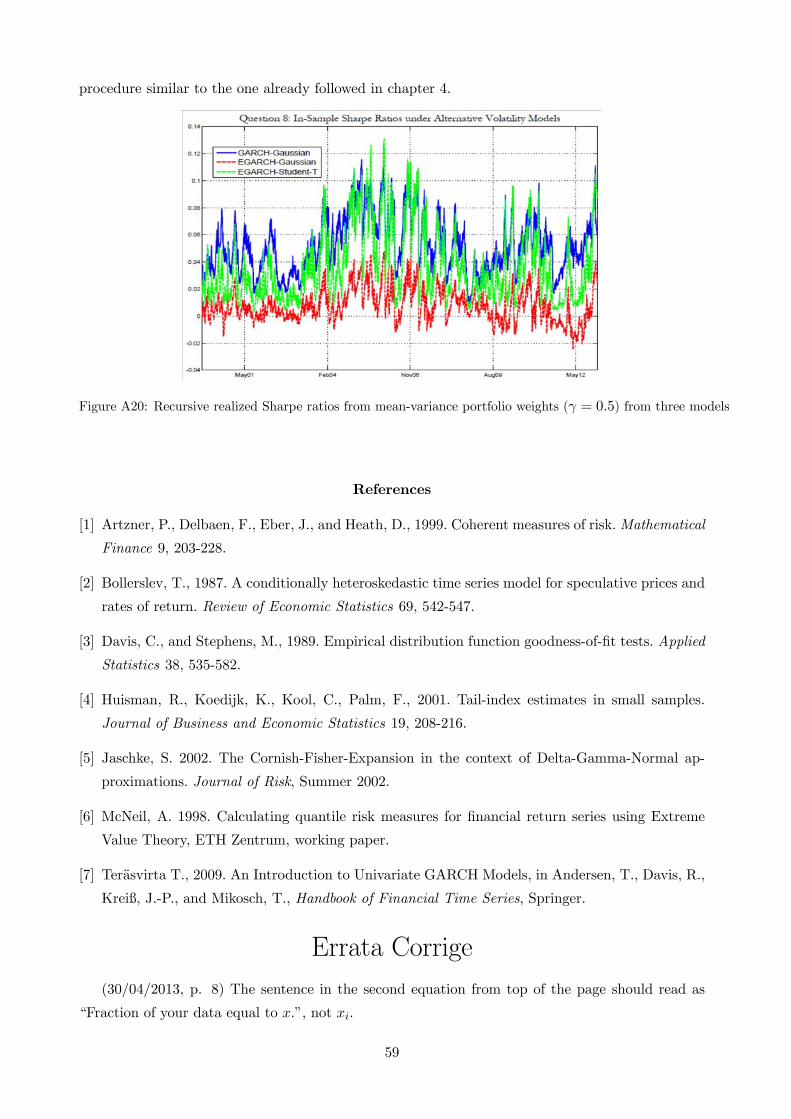
procedure similar to the one already followed in chapter 4.
Figure A20: Recursive realized Sharpe ratios from mean-variance portfolio weights ( = 05) from three models
References
[1] Artzner, P., Delbaen, F., Eber, J., and Heath, D., 1999. Coherent measures of risk.Mathematical
Finance 9, 203-228.
[2] Bollerslev, T., 1987. A conditionally heteroskedastic time series model for speculative prices and
rates of return. Review of Economic Statistics 69, 542-547.
[3] Davis, C., and Stephens, M., 1989. Empirical distribution function goodness-of-fit tests. Applied
Statistics 38, 535-582.
[4] Huisman, R., Koedijk, K., Kool, C., Palm, F., 2001. Tail-index estimates in small samples.
Journal of Business and Economic Statistics 19, 208-216.
[5] Jaschke, S. 2002. The Cornish-Fisher-Expansion in the context of Delta-Gamma-Normal ap-
proximations. Journal of Risk, Summer 2002.
[6] McNeil, A. 1998. Calculating quantile risk measures for financial return series using Extreme
Value Theory, ETH Zentrum, working paper.
[7] Terasvirta T., 2009. An Introduction to Univariate GARCH Models, in Andersen, T., Davis, R.,
Kreiß, J.-P., and Mikosch, T., Handbook of Financial Time Series, Springer.
Errata Corrige
(30/04/2013, p. 8) The sentence in the second equation from top of the page should read as
“Fraction of your data equal to .”, not .
59

(30/04/2013, p. 10) Towards the end of the page, the sentence should read as “This means that
the right tail of the empirical distribution of S&P 500 returns is thicker than the normal tail”.
(30/04/2013, p. 14) A new footnote 21 has been added to explain what the model of reference
is at pp. 14-16.
(30/04/2013, p. 15) A −3 has been added in the equation providing the moment matchingcondition for 2 and one spurious equal sign removed from 2
−2 = b2.
(30/04/2013, p. 46 and workout Matlab code posted on the web) The formula (1 + 05) +
has been now used to compute the GJR stationarity measure (there would be reasons not to, but it
is easier this way; thanks M. Fiorani-Gallotta for pointing out the insidious inconsistency). In this
case, 0(1 + 05× 01381) + 09131 = 09131 of course.(07/05/2013, p. 8) In equation (4) the pedices labelling the two kernel densities as “Box” and
“Triangular” have been switched.
(07/05/2013, p. 23) −1 (670) should be −1 (670)
60