Clemson UniversityTigerPrints

All Theses Theses

12-2009

MODELING THE COOLING PHASE OFTHE LENS MOLDING PROCESSSaravanan KannanClemson University, saravanan4u@gmail.com

Follow this and additional works at: https://tigerprints.clemson.edu/all_theses

Part of the Engineering Mechanics Commons

This Thesis is brought to you for free and open access by the Theses at TigerPrints. It has been accepted for inclusion in All Theses by an authorizedadministrator of TigerPrints. For more information, please contact kokeefe@clemson.edu.

Recommended CitationKannan, Saravanan, "MODELING THE COOLING PHASE OF THE LENS MOLDING PROCESS" (2009). All Theses. 705.https://tigerprints.clemson.edu/all_theses/705

i

MODELING THE COOLING PHASE OF THE LENS MOLDING PROCESS

A Thesis

Presented to

the Graduate School of

Clemson University

In Partial Fulfillment

of the Requirements for the Degree Master of Science

Mechanical Engineering

by

Saravanan Kannan

December 2009

Accepted by:

Dr. Vincent Y. Blouin, Committee Chair Dr. Paul F. Joseph

Dr. Richard S. Miller Dr. Kathleen A. Richardson

Dr. Xiangchun Xuan

ii

ABSTRACT

The lens molding process is a relatively new technique used to manufacture

lenses, in particular, high precision aspheric lenses. In order to achieve the desired size

and shape of the lens, the cooling process after pressing must be controlled precisely

because of the time and temperature dependent viscoelastic behavior of glass near and

below the molding temperature. This thesis gives a detailed description of a three-

dimensional computational model for analyzing the cooling phase of the lens molding

process. Conduction, convection and radiation are considered in the model by coupling a

computational fluid dynamics analysis of the flow of nitrogen through the system and a

transient heat transfer finite element analysis of the assembly. An iterative process

between the fluid flow analysis and the thermal analysis is used to account for their

interdependency. The model is calibrated and validated by direct comparison with the

experimental results. Various parametric studies are performed to study the effect of

several unknown parameters and design parameters on the accuracy of the numerical

model. It was found that the model depends significantly on the unknown properties such

as thermal contact conductance values and radiation properties, which should therefore be

the subject of further investigation. This three-dimensional model can be used to extract

the boundary conditions for a parallel study involving a more detailed two-dimensional

axisymmetric sub-model of the lens and molds. The validity of two-dimensional

axisymmetry assumption is verified from the results obtained through the three-

dimensional model‟s simulations.

iii

DEDICATION

This thesis is dedicated to my parents Mr. Kannan Arunachalam and Mrs.

Thenmozhi Kannan.

iv

ACKNOWLEDGMENTS

I would like to thank my advisor, Dr. Vincent Blouin for his continuous support

and guidance throughout my Masters program. His advice and constant encouragement

helped me in finishing my thesis in numerous ways.

I would also like to thank Dr. Paul Joseph, Dr. Kathleen Richardson, Dr. Richard

Miller and Dr. Xiangchun Xuan for their valuable inputs and their suggestions.

I would also like to thank Edmund Optics, the lens manufacturer for their

financial support.

Last but not least, I would like to thank my parents Kannan Arunachalam and

Thenmozhi Kannan and my brothers Karthikeyan and Siva and all my friends for their

support and love throughout my life.

v

TABLE OF CONTENTS

Page

TITLE PAGE ................................................................................................................... i

ABSTRACT .................................................................................................................... ii

DEDICATION ............................................................................................................... iii

ACKNOWLEDGMENTS .............................................................................................. iv

LIST OF TABLES ....................................................................................................... viii

LIST OF FIGURES ........................................................................................................ ix

CHAPTER

1. INTRODUCTION ......................................................................................... 1

1.1 Background ....................................................................................... 1 1.2 Research Objectives .......................................................................... 4

1.3 Literature Study ................................................................................. 4

1.4 Thesis Outline .................................................................................... 8

2. COMPRESSION MOLDING PROCESS ................................................... 10

2.1 Description of the Molding Process ................................................ 10

2.2 Detailed Description of the Cooling Process ................................... 16

3. FINITE ELEMENT NUMERICAL MODEL ............................................. 18

3.1 Model Description ........................................................................... 18

3.2 Material Properties .......................................................................... 20 3.3 Analysis procedure .......................................................................... 20

3.4 Initial Conditions ............................................................................. 21

3.5 Input Heat Fluxes ............................................................................ 22 3.6 Radiation ......................................................................................... 23

3.7 Meshing ........................................................................................... 25

3.8 Assumptions and Limitations .......................................................... 26

3.9 Thermal Contact Conductance ........................................................ 26

3.10 Example Simulation results ........................................................... 27

vi

Table of Contents (Continued)

Page

4. COMPUTATIONAL FLUID DYNAMICS MODEL ................................ 29

4.1 Background ..................................................................................... 29

4.2 CFD Model of a Single Cooling Channel ....................................... 30

4.2.1 Geometry of the Channel ..................................................... 30

4.2.2 Properties of the Fluid ......................................................... 31 4.2.3 Initial and Boundary Conditions .......................................... 31

4.2.4 Solution Parameters ............................................................. 32

4.2.5 Results ................................................................................. 33

4.2.6 Analytical Validation ........................................................... 35

4.3 CFD Model of the Entire Fluid Domain .......................................... 36

4.3.1 Geometry ............................................................................. 36

4.3.2 Example Simulation Results ................................................ 37

4.3.3 Design of Experiments ........................................................ 39

5. COUPLING FEA AND CFD ...................................................................... 40

5.1 Introduction….... ............................................................................. 40

5.2 Interaction between FEA and CFD ................................................. 40

5.3 Coupled Solver for ABAQUS and FLUENT .................................. 41

5.4 Example Simulation Results ............................................................ 44

6. PARAMETRIC STUDIES .......................................................................... 46

6.1 Parametric Study on Contact Conductance value „h‟ ...................... 46 6.2 Parametric Study on Emissivity and Ambient Temperature ........... 51

6.3 Effect of Nitrogen (coolant) Temperature ....................................... 54 6.4 Parametric study on Number of Increments between

FLUENT and ABAQUS .............................................................. 55

7. EXTRACTION OF BOUNDARY CONDITIONS..................................... 58

7.1 Transferring Data from the 3D Model to the 2D

Axisymmetric Model ................................................................. 58

7.2 Heat Flux Results throughout the Assembly ….... .......................... 64

8. CONCLUSION AND FUTURE WORK .................................................... 67

8.1 Conclusion ....................................................................................... 67

8.2 Future Work .................................................................................... 68

vii

Table of Contents (Continued)

Page

APPENDICES ............................................................................................................... 70

A: MATLAB code for interacting between ABAQUS and

Fluent ..................................................................................................... 71

REFERENCES .............................................................................................................. 83

viii

LIST OF TABLES

Table Page

3.1 Material properties ...................................................................................... 20

4.1 Properties of the coolant nitrogen ................................................................ 31

4.2 Boundary types at first increment ................................................................ 32

6.1 Contact conductance (h) values for various contact surfaces

and pressures ........................................................................................ 47

ix

LIST OF FIGURES

Figure Page

1.1 Spherical aberration in a lens ........................................................................ 2

1.2 No aberration in an aspheric lens .................................................................. 2

2.1 Toshiba Molding Machine .......................................................................... 10

2.2 Molding Machine Assembly ....................................................................... 11

2.3 Schematic model of the molding assembly during cooling ......................... 12

2.4 Different Stages of Lens molding process ................................................... 14

2.5 Schematics of four stages of a glass lens molding process ......................... 15

2.6 Two different stages of cooling phase in the molding process .................... 17

3.1 One-quarter ABAQUS model of the Molding Assembly............................ 19

3.2 See-through model of the one-eighth model of the molding assembly

in ABAQUS .......................................................................................... 21

3.3 Cooling Plate ............................................................................................... 23

3.4 Surfaces where convection and radiation condition are defined ................. 25

3.5 Figure 3.5: Simulation output, temperature distribution through the assembly at various times of the cooling phase.................. 28

4.1 Nitrogen flow inside the assembly with their flow rates ............................. 29

4.2 Cooling channel with boundary conditions in GAMBIT ............................ 30

4.3 Contour of heat flux along the length of the channel .................................. 34

4.4 Heat flux along the channel length for channel ........................................... 35

4.5 Model used by Benet Lab for heat flux calculation ..................................... 37

4.6 Contour of surface heat transfer coefficient ................................................ 38

x

4.7 Streamlines throughout and around the assembly ....................................... 38

5.1 Schematic representation of the interaction between CFD and FEA .......... 41

5.2 Schematic representation of the MATLAB code as a coupled

solver between FEA and CFD ............................................................... 42

5.3 Algorithmic representation of the interaction between CFD and FEA by

Matlab .................................................................................................... 43

5.4 Simulation output, temperature distribution through the assembly

at various times of the cooling phase .................................................... 44

5.5 Temperature profile at the end of 300 seconds ............................................ 45

6.1 Temperature as a function of time for different h values with an

emissivity of 0.55 and ambient temperature of 250 deg C .......................... 49

6.2 Temperature after 300 seconds of cooling at the location of the

thermocouple for different h values....................................................... 50

6.3 Temperature as a function of time at Thermocouples with respect

to various emissivities for a constant ambient temperature

of 200 deg C .......................................................................................... 51

6.4 Temperature as a function of time at Thermocouples with respect

to various emissivities for a constant ambient temperature

of 250 deg C .......................................................................................... 52

6.5 Temperature as a function of time at Thermocouples with respect to various emissivities for a constant ambient temperature

of 300 deg C .......................................................................................... 53

6.6 Temperature along the length of the cooling channel for various

incremental procedures. ......................................................................... 55

6.7 Heat flux along the length of the channel for the five increments in a five

incremental procedure ........................................................................... 56

6.8 Temperature at a point in the cooling channel for various incremental

Procedures ............................................................................................. 57

xi

List of Figures (Continued)

Figure Page

7.1 3D model and boundary of the 2D axisymmetric model showing

the upper and lower tools and lens ........................................................ 58

7.2 Tool showing the edges for which the temperatures are plotted

in Figure 7.3 .......................................................................................... 59

7.3 Temperature as a function of time for various edges in the tool

shown in Figure 7.2 ............................................................................... 60

7.4 Tool and lens showing the edges in yz-plane for which the

temperatures are plotted in Figure 7.5 ................................................... 61

7.5 Temperature as a function of time for various edges in the tool

and the lens shown in Figure 7.4 ........................................................... 61

7.6 Tool and lens showing the points where heat fluxes are plotted

in Figure 7.7 .......................................................................................... 62

7.7 Heat flux per area as a function of time for various elements

in the tool and the lens shown in Figure 7.6 .......................................... 62

7.8 7.8: Tool and lens showing the points where heat fluxes are

plotted in Figure.7.9 .............................................................................. 63

7.9 Heat flux per area as a function of time for various nodes (points) in the tool and the lens shown in Figure 7.8 ......................................... 63

7.10 Heat flux vector in the whole model ........................................................... 64

7.11 Heat flux vectors on a section on the xz-plane ............................................ 65

7.12 Heat flux vectors on a section cut on a plane rotated 30degrees

about the z-axis from the xz-plane (through the cooling channels) ....... 65

7.13 Heat flux vectors for a section on a plane parallel to the yz-plane through the middle of the lens (a) after 10 seconds ............................... 66

1

CHAPTER ONE

INTRODUCTION

1.1 Background

Glass lenses have been used in the field of high resolution digital cameras, DVD

players and recorders. Spherical lenses are the most common type of lenses. Spherical

surfaces are generally created by polishing the lens preform between convex and concave

parts of intended radius of curvature. The word “preform” refers to the initial glass work

piece that is then formed into the final lens either through machining, grinding and

polishing or molding.

One of the major drawbacks of spherical lenses is spherical aberration, i.e., they

cannot focus the light into a single point as illustrated in Figure 1.1. Parallel rays that pass

through the central region of a spherical lens focus farther away than the light rays that

passes through the edges of the lens. The result is a focal region, which may produce a

blurry image. In most applications, this problem is corrected by having multiple

spherical lenses placed in series to compensate for the error introduced by a single lens.

This multiple-lens assembly, however, results in alignment and mounting complexities,

higher cost and higher weight.

Aspheric lenses have one or both surfaces that do not conform to a sphere and can

theoretically focus all the incoming light rays on to a single point on the lens axis as

illustrated in Figure 1.2. Aspheric lenses are therefore more efficient, since they do not

need addition corrective lenses making devices lighter, smaller and potentially cheaper.

2

High precision lenses find their application in medical and military equipments, scientific

testing devices and collision avoidance devices.

Figure 1.1: Spherical aberration in a lens

Figure 1.2: No aberration in an aspheric lens

Lens molding technology was developed to mass-produce aspheric lenses for

larger lens systems, from 2 to 60 mm in diameter. Aspherical lenses can also be

manufactured by precision ground method whereby the glass surface is directly grounded

3

with a grinding device. Molded aspheres are produced by heating the preform until it

becomes soft and then pressing it between aspheric dies. To manufacture a molded

asphere, a tool (i.e., mold) must be created, which involves a complex and expensive

iterative process. High cost of manufacturing aspheric elements has prevented their

common use by lens designers and optical engineers.

Compression molding offers a promising approach for large volume, cost

effective manufacturing of precision aspheric lenses which otherwise is difficult to make

using conventional lens fabrication techniques. One of the problems the manufacturers

are facing is that after making a few hundred lenses, cracks appear at the surface of the

molds (mold coating degradation).

Edmund Optics partnered with Clemson University and Benet Laboratories, a

U.S. Army research facility, to develop assembly technology for molded aspheric

systems. The goal of this project was to minimize the time and cost of producing aspheric

lenses. Several research teams worked in parallel on this project to address several

aspects of the glass molding process such as the use of finite element analysis (FEA)

models to predict the lens final size and shape, and identify the material parameters

critical to a successful interaction of the glass and mold. As part of this project,

Ananthasayanam [1] developed a two-dimensional (2D) axisymmetric Finite Element

model of on the lens and dies for the entire molding process including all stages, namely,

heating, soaking, pressing, cooling, and release. The research presented in this thesis

focuses on the development of a three-dimensional (3D) Finite Element model of the

entire assembly during the cooling stage governed by the flow of nitrogen through

4

cooling channels within the assembly. The overarching goal was to use the output of the

3D model, namely, temperature boundary condition and heat fluxes of the cooling stage,

as input to the 2D model.

1.2 Research Objectives

The objectives of the research reported in this thesis are:

- Develop a three-dimensional transient heat transfer numerical model of the cooling

stage using an incremental procedure coupling Finite Element Analysis (FEA) for the

temperature analysis and Computational Fluid Dynamics (CFD) for the analysis of

the fluid flow of nitrogen;

- Perform parametric studies to investigate the influence of parameters related to the

numerical process (such as partitioning of the cooling channels and number of

increments) and parameters for which we have low confidence (such as input

nitrogen temperature, thermal contact conductance values and radiation parameters);

- Extract information such as heat fluxes and temperature boundary conditions needed

for the parallel two-dimensional axisymmetric numerical study focused on the

prediction of the final size and shape of the lens.

1.3 Literature Study

Numerical modeling of molding processes

Compression molding offers a promising approach for large volume, cost

effective manufacturing of precision aspheric lenses which otherwise is difficult to make

using conventional lens fabrication techniques. Yana et al. [2] have modeled the high

temperature glass lens molding process by coupling heat transfer and viscous

5

deformation analysis. In their study a two-step pressing process is proposed according to

the non-linear thermal expansion characteristics of glass. The results concluded that

incomplete heating of glass not only increases the pressing load at the beginning of

pressing, but also leads to non uniformity in viscous deformation and geometrical error of

the glass component. Molding process simulations were carried out using a FEM

program DEFORM – 3D. A computational model for the cooling phase of the injection

molding process was developed by Smitha and Wrobela [3]. The whole geometry was

created in I-DEAS and then imported into GAMBIT where all the initial and boundary

conditions were applied and then exported to FLUENT for analysis. The use of

computational model allows the monitoring of maximum and minimum temperatures and

temperature contour plots on any surface. The results generated through the model can be

used to evaluate a potential mold cooling configuration in advance of tool manufacture.

Sridhar and Nahr [4] studied the effect of temperature dependent thermal

properties on process parameter prediction in injection molding. The results obtained

from the simulations are compared with those of constant thermal properties such as

contact thermal conductance and specific heat. Based on the simulation results it is found

that the bulk temperature, defined as the velocity weighted average temperature

calculated based on variable thermal conductivity and specific heat will give a shorter

cycle time than those based on constant values.

As mentioned earlier, Ananthasayanam [1] developed a two-dimensional

axisymmetric coupled temperature-displacement model of the glass molding process

using ABAQUS to simulate the whole process of lens forming and to predict the final

6

shape/size of the lens. The results showed that the primary cause of the deviation of the

lens profile was due to structural relaxation of the glass, time-temperature dependence of

viscoelastic behavior of glass and thermal expansion behavior of the molds.

Modeling Fluid-structure-thermal interactions

Bilgen [5] conducted a numerical and experimental study of a conjugate heat

transfer problem by conduction and natural convection on a heated vertical wall. The

author made an assumption that the wall is subjected to a uniform heat flux on one side

and cooled on both sides by natural convection of surrounding air. The equations of mass,

momentum and energy conservations are solved by a control volume method – Simpler

algorithm. The results obtained showed that the interaction of conduction with natural

convection on a heated vertical wall results in reducing the wall temperature and in

making it nearly isothermal along the wall.

Zhou and Li [6] developed a computer simulation for three-dimensional mold

heat transfer of the television panel pressing process. Two analyses were done in this

simulation, one three-dimensional boundary element method for the mold region and a

finite-difference method with a variable mesh for the melt region. These two analyses

were iteratively coupled so as to match the temperature and heat flux at the mold melt

interface. The iterative procedure starts with assuming the mold-melt interface

temperature distribution and carrying out the part melt analysis to determine the heat flux

variation with time along the mold-melt interface. After determining the cycle average

flux values using heat flux distribution mold analysis is performed to obtain the

temperature distribution along the interface. If the interface temperature is in close

7

agreement with that assumed for the melt analysis the iterative procedure is stopped,

otherwise the procedure is repeated again. The authors found that the simulation package

is very suitable as a tool in the optimization of mold and processing design, and is

currently used to optimize a production line.

Lanoye et al. [7] studied the interaction between blood flow and the vessel wall

while studying the vascular blood flow. A set of solutions was obtained through the

implementation of a fluid-structure-interaction scheme. They established a coupling

between fluid solver software Fluent 6.2 and structural solver software Abaqus 6.5

similar to the coupling presented in this thesis.

Lin et al. [8] studied a fully 3D simulation of mold temperature variations based

on FEA and Finite Volume Method (FVM) implemented in a parallel computation

scheme for lens molding. The mold temperature and melt temperature are solved in a

coupled manner and obtained simultaneously. Combined space and time parallelization

offer the possibility of adapting to characteristics of the parallel computer used, which

results in high efficiency. They concluded that the FEA-FVM combined approach with

parallel scheme compares well with measured experimental values. The parallel scheme

offers much less computational cost than the standard analysis on a single computer.

Experimental characterization of cooling processes

Peng and Wang [9] experimentally investigated the heat transfer characteristics

and cooling performance of rectangular shaped microgrooves machined into stainless

steel plates. The influence of liquid velocity, sub-cooling, property variations and micro

channel geometric configuration on the heat transfer behavior and cooling performance

8

were analyzed experimentally. The results of their study concluded that the heat transfer

performance and the cooling characteristics were enhanced as the channel number

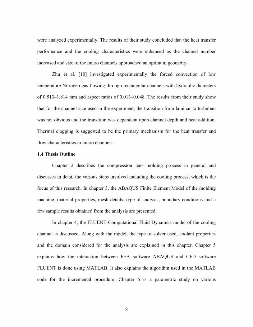
increased and size of the micro channels approached an optimum geometry.

Zhu et al. [10] investigated experimentally the forced convection of low

temperature Nitrogen gas flowing through rectangular channels with hydraulic diameters

of 0.513–1.814 mm and aspect ratios of 0.013–0.048. The results from their study show

that for the channel size used in the experiment, the transition from laminar to turbulent

was not obvious and the transition was dependent upon channel depth and heat addition.

Thermal clogging is suggested to be the primary mechanism for the heat transfer and

flow characteristics in micro channels.

1.4 Thesis Outline

Chapter 2 describes the compression lens molding process in general and

discusses in detail the various steps involved including the cooling process, which is the

focus of this research. In chapter 3, the ABAQUS Finite Element Model of the molding

machine, material properties, mesh details, type of analysis, boundary conditions and a

few sample results obtained from the analysis are presented.

In chapter 4, the FLUENT Computational Fluid Dynamics model of the cooling

channel is discussed. Along with the model, the type of solver used, coolant properties

and the domain considered for the analysis are explained in this chapter. Chapter 5

explains how the interaction between FEA software ABAQUS and CFD software

FLUENT is done using MATLAB. It also explains the algorithm used in the MATLAB

code for the incremental procedure. Chapter 6 is a parametric study on various

9

parameters and their effects on the cooling rate. Results obtained from the studies are

discussed in detail. Chapter 7 explains how the temperature as well as heat flux can be

given as boundary conditions to the parallel study discussed in section 1.1.In chapter 8

the research study is summarized with important conclusions based on the simulations

and recommendations for future work are made.

10

CHAPTER TWO

COMPRESSION MOLDING PROCESS

2.1 Description of the Molding Process

Compression molding is a form of molding process in which the material to be

molded is generally preheated and then placed in a heated mold cavity. The compression

molding machine consists of a cylindrical assembly made of several parts as shown in

Figures 2.1 and 2.2. The lens (i.e., glass preform) is compressed between the upper and

lower sub-assemblies, both of which consist of a die holder, a mold, a zinc plate separator

(only in lower sub-assembly), and a cooling plate.

Figure 2.1. Toshiba Molding Machine

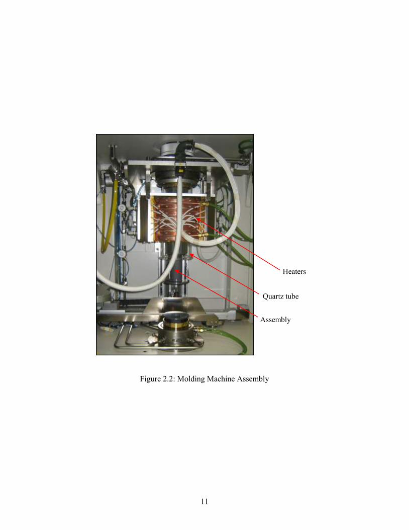
Figure 2.1 shows the GMP–311VA Toshiba molding machine owned by Edmund

Optics for manufacturing aspherical lenses.

11

Figure 2.2: Molding Machine Assembly

Heaters

Assembly

Quartz tube

12

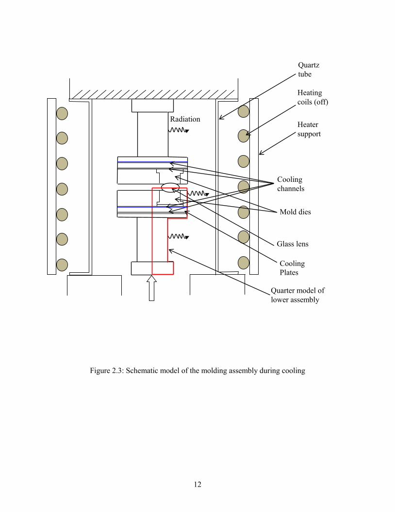
Figure 2.3: Schematic model of the molding assembly during cooling

Quarter model of

lower assembly

Heating

coils (off)

Quartz

tube

Heater

support

Glass lens

Radiation

Mold dies

Cooling

channels

Cooling

Plates

13

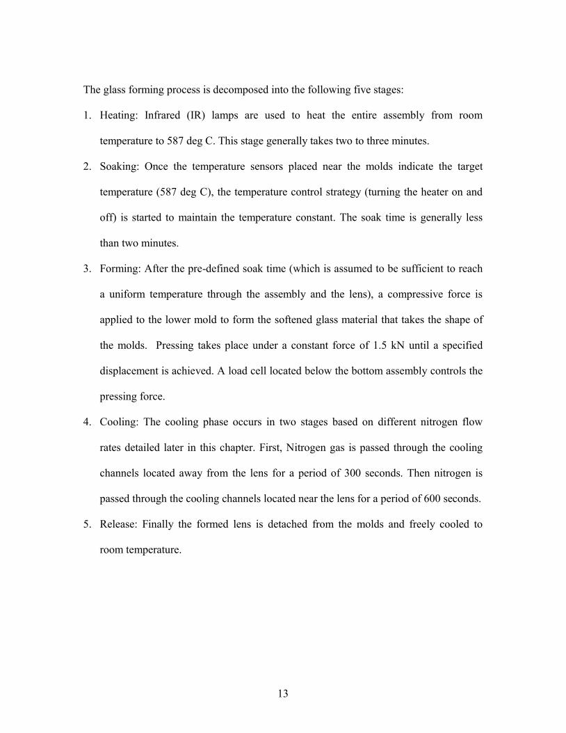
The glass forming process is decomposed into the following five stages:

1. Heating: Infrared (IR) lamps are used to heat the entire assembly from room

temperature to 587 deg C. This stage generally takes two to three minutes.

2. Soaking: Once the temperature sensors placed near the molds indicate the target

temperature (587 deg C), the temperature control strategy (turning the heater on and

off) is started to maintain the temperature constant. The soak time is generally less

than two minutes.

3. Forming: After the pre-defined soak time (which is assumed to be sufficient to reach

a uniform temperature through the assembly and the lens), a compressive force is

applied to the lower mold to form the softened glass material that takes the shape of

the molds. Pressing takes place under a constant force of 1.5 kN until a specified

displacement is achieved. A load cell located below the bottom assembly controls the

pressing force.

4. Cooling: The cooling phase occurs in two stages based on different nitrogen flow

rates detailed later in this chapter. First, Nitrogen gas is passed through the cooling

channels located away from the lens for a period of 300 seconds. Then nitrogen is

passed through the cooling channels located near the lens for a period of 600 seconds.

5. Release: Finally the formed lens is detached from the molds and freely cooled to

room temperature.

14

The process data obtained from the manufacturer is shown in the Figure 2.4.

Figure 2.4: Different Stages of Lens molding process

Rapid Cooling

Stage Slow Cooling

15

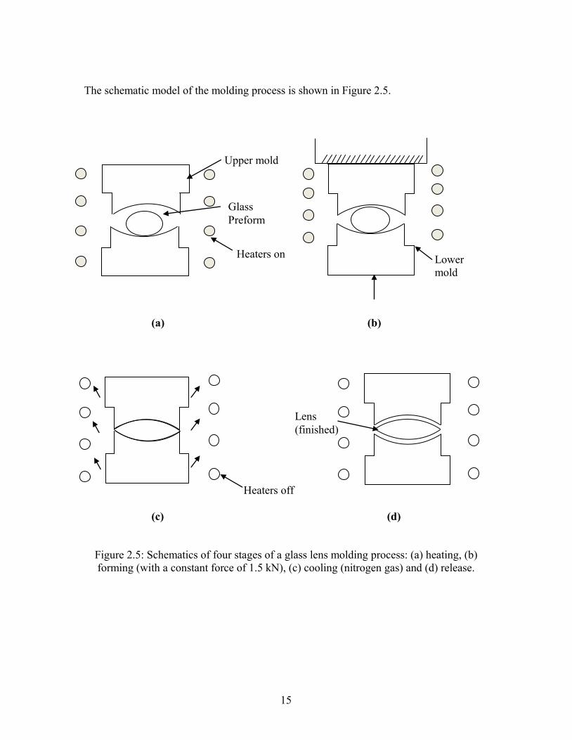
The schematic model of the molding process is shown in Figure 2.5.

(a) (b)

(c) (d)

Figure 2.5: Schematics of four stages of a glass lens molding process: (a) heating, (b)

forming (with a constant force of 1.5 kN), (c) cooling (nitrogen gas) and (d) release.

Heaters on

Upper mold

Glass

Preform

Heaters off

Lens

(finished)

Lower

mold

16

2.2 Detailed Description of the Cooling Process

During the cooling process, the heat is removed by the three main heat transfer

mechanisms, i.e., conduction, convection and radiation. The heat is removed from the

glass mainly by conduction of heat into the tools and mold dies. Heat is removed from

the mold dies by convection through the cooling channels and radiation to the

environment. By controlling the nitrogen flow rate through the cooling channels, initial

slow cooling is performed to lower the glass temperature below its transformation

temperature followed by fast cooling. A constant load is maintained on the formed lens

during this step. The lens is finally released from the molds close to room temperature

and is allowed to cool to the ambient.

The cooling channels closer to the lens (hereafter referred to as upper cooling

channels) are formed by the gap between the mold dies and the cooling plate. The cooling

channels away from the lens (hereafter referred to as lower cooling channels) are formed

by the gap between the cooling plates and die holders. More details about the cooling

channels are given in Chapter 3.

17

Figure 2.6: Two different stages of cooling phase in the molding process

As explained earlier, there are two stages of cooling, slow cooling and rapid

cooling. During slow cooling the nitrogen flows around the assembly in addition to the

lower cooling channels. The rapid cooling occurs in the second stage of the cooling phase

where the entire assembly is cooled down with nitrogen in approximately 10 minutes. In

this stage the nitrogen flow around the assembly is turned off and only the upper cooling

channels are turned on at a high rate.

18

CHAPTER THREE

FINITE ELEMENT NUMERICAL MODEL

3.1 Model Description

Numerical Finite Element Method (FEM) has routinely been used in the

manufacturing industry to study, analyze, develop, improve and optimize manufacturing

process performance. With the advent of the advanced commercial FEM codes and

computing hardware it is possible to realistically simulate and observe process variables

that are difficult or even impossible to measure from experiments, for example in case of

lens molding it includes among others: temperature distribution in glass, residual stress

distribution, etc.

The 3D model of the molding assembly was done in ABAQUS, a commercial

software package for Finite Element Analysis [11]. Symmetry is taken into account to

first reduce the size of the model to a quarter of the assembly as shown in Figure 3.1. The

model was then reduced further to an eighth of the assembly by assuming vertical

symmetry. That is the shape of the lens and the thermal behavior are assumed symmetric

about the middle XY-plane. The quarter model of Figure 3.1 shows the molding

assembly which is made up of different parts as follows:

Lens

Spacer

Tools (lower and upper)

Cooling Plates (lower and upper)

Die Holders (lower and upper)

Mold Dies

Nitrogen Tubes

19

Separators

Figure 3.1: One-quarter ABAQUS model of the Molding Assembly and materials in

parentheses

Y X

Z

20

3.2 Material Properties

Table 3.1 shows the properties of all the materials used in the modeling of the

molding machine.

Table 3.1: Material Properties (Refer to Figure 3.1)

Property Glass J05 M45 (Nickel

Binder)

FHR96 (Cemented

Carbide)

Si3N4 (Silicon

nitride)

Conductivity

(W/(m.K)) 1.126 63 42 54 15

Density (kg/m3)

2000 14650 14400 17600 3200

Poisson's

Ratio 0.25 0.2 0.22 0.28 0.27

Expansion

Coefficient

(/C)

8.1x10-6 4.6 10-6 at 400 C

4.8 10-6 at 600 C

5.5 10-6 at 400 C

5.9 10-6 at 600 C

5.4 10-6 at 400 C

5.5 10-6 at 600 C

1.8 10-6 at 400 C

2.1 10-6 at 600 C

Young's

Modulus (N/m2)

1.0e1E+11 6.5E+11 5E+11 3.5E+11 2.91E+11

Specific Heat

(J/(kg-K)) 200 400 400 400 711

3.3 Analysis procedure

In ABAQUS, a transient heat transfer analysis was done for all the simulations.

This analysis is used to model the solid body heat conduction and temperature-dependent

conductivity, convection and radiation boundary conditions. In this simulation the forced

convection part was done using FLUENT, a 3D Computational Fluid Dynamics (CFD)

based tool from ANSYS [12].

21

3.4 Initial Conditions

The initial temperature field is defined as 587 deg C everywhere in the model.

This is the temperature that is maintained through the whole model during the pressing

phase just before the cooling starts. .During the starting of the cooling phase, the top and

bottom molds of the assembly are in a closed position and is maintained in that position

for the first phase of cooling (300 seconds).

Figure 3.2: See-through model of the one-eighth model of the molding assembly in

ABAQUS

Cooling Plates

Mold Dies

Nitrogen Tubes

Die Holders

Cooling Channels

22

The red arrows in Figure 3.2 indicate the path of nitrogen flow through the lower

cooling channels between the cooling plate and the die holder. The cooling channels

closer to the lens are formed by the gap between the mold dies and the cooling plates.

The cooling channels away from the lens are formed by the gap between the cooling

plates and the die holders.

3.5 Input Heat Fluxes

Heat transfer analysis is done in ABAQUS by defining heat fluxes as negative

thermal loads on specific surfaces and running the simulation for the first cooling period

of 300 seconds. The thermal loads are negative since they draw the heat out of the

assembly to cool. Heat fluxes defined on the cooling channels were found out by taking

the fluid domain in the cooling channels alone into the account (detailed explanation is

given in chapter 4), whereas heat fluxes defined on the surfaces other than the cooling

channels, such as the outer surfaces of the die holders and cooling plates are calculated by

Dan Cler, from Benet Laboratories, a research partner in this project

In order to account for the temperature-dependency of the heat fluxes during the

transient heat transfer, the fluxes are updated at predefined specific times during the

simulation. For instance, the 300-second simulation can be divided into 5 increments of

60 seconds with an update at the start of each increment.

23

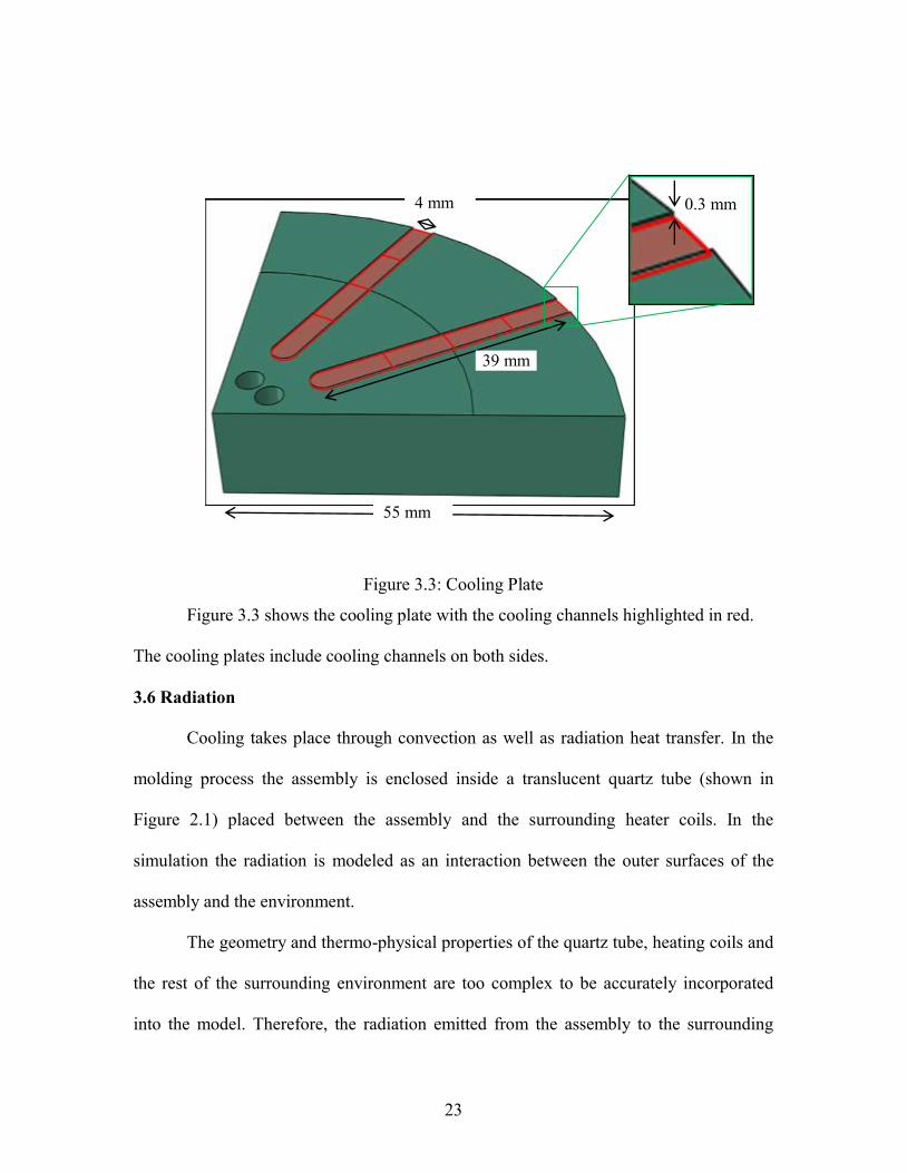
Figure 3.3: Cooling Plate

Figure 3.3 shows the cooling plate with the cooling channels highlighted in red.

The cooling plates include cooling channels on both sides.

3.6 Radiation

Cooling takes place through convection as well as radiation heat transfer. In the

molding process the assembly is enclosed inside a translucent quartz tube (shown in

Figure 2.1) placed between the assembly and the surrounding heater coils. In the

simulation the radiation is modeled as an interaction between the outer surfaces of the

assembly and the environment.

The geometry and thermo-physical properties of the quartz tube, heating coils and

the rest of the surrounding environment are too complex to be accurately incorporated

into the model. Therefore, the radiation emitted from the assembly to the surrounding

4 mm

39 mm

0.3 mm

55 mm

24

environment is defined by an effective environment temperature, 0 , referred to as the

non-reflective environment temperature or the ambient temperature. Since this effective

temperature and the emissivity of the materials are unknown a parametric study,

described in the next section, was performed to determine the appropriate values to match

the experimental measurements.

In ABAQUS, the radiation heat flux per unit area q (W/m2) is defined as

4 0 4( ) ( )z zq

where σ is the Stefan-Boltzmann constant, ε is the emissivity of the surface of interest,

0 is the ambient temperature (also referred to as the temperature of the non-reflecting

environment), is the temperature of the surface of interest and z is the absolute zero

temperature.

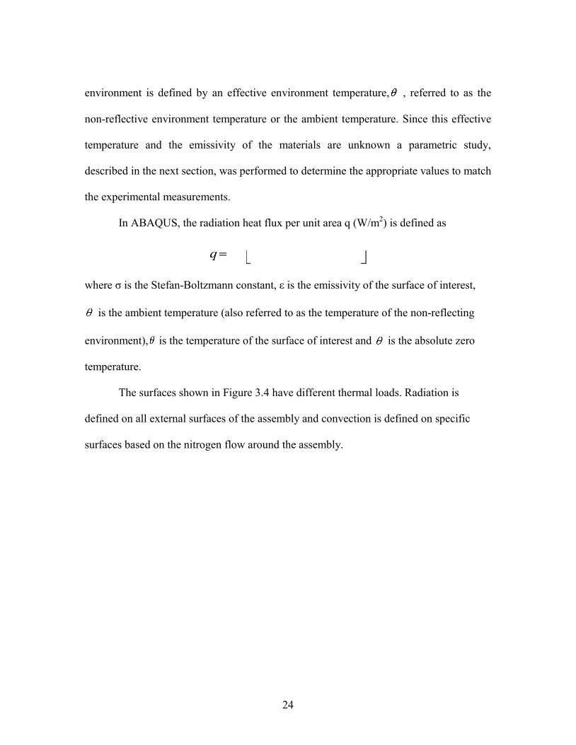
The surfaces shown in Figure 3.4 have different thermal loads. Radiation is

defined on all external surfaces of the assembly and convection is defined on specific

surfaces based on the nitrogen flow around the assembly.

25

Figure 3.4: Surfaces where convection and radiation condition are defined

3.7 Meshing

The finite element mesh includes linear tetrahedral and hexahedral elements. The

entire assembly consists of about 53,000 elements (clock time for a single simulation

ranges from 1 hour to 2.5 hours). To study the effect of meshing on the results a finer

mesh of 100,000 elements was tested. The results of both cases were matching within 1.0

deg C in temperature after 300 seconds of simulation. Therefore, in order to maintain the

computation time as low as possible, the coarser mesh (53,000 elements) was assumed to

be sufficient for all simulations.

Radiation & Convection

Point where temperature measurements are taken

1

2

4

5

6

7

8

9

10

11

12

No Heat Flux Convection Radiation

3

26

3.8 Assumptions and Limitations

i. The xz-plane and yz-plane are considered as planes of symmetry in order to

reduce the size of the sample to one-quarter of the assembly.

ii. Differences between the top and bottom halves of the assembly are neglected

taking the xy-plane as a plane of symmetry to further reduce the model to one-

eighth of the assembly (shown in Figure 3.2).

iii. Non-uniformity of pressure in the radial direction is neglected. Therefore, surface

conductance values are assumed uniform throughout the assembly (discussed in

the next section).

iv. In defining radiation, although the heating elements (coils and support) cool down

during the cooling period of 300 seconds, the ambient temperature of the radiation

model, which represents the inside surface of the heating elements is maintained

constant throughout the cooling period.

3.9 Thermal Contact Conductance

Thermal Contact Conductance (TCC) h, is the ratio of the heat flux (Q/A) to the

temperature drop across the interface of two materials in contact. It is recognized that

thermal contact conductance is a function of several parameters, the dominant ones being

the type of contacting materials, the macro- and micro-geometry of the contacting

surfaces, the temperature, the interfacial pressure, the type of lubricant or contaminant

and its thickness [13, 14]. In processes involving high temperature, high pressure and

various material-material interactions this contact conductance plays a critical role. When

two materials are in contact with each other the actual contact takes place only at a few

27

points where heat transfer takes place. Even if the pressure is increased by several orders

of magnitude the actual contact area is generally still much less than the nominal contact

area.

In ABAQUS, the TCC values were implemented to define conductive heat

transfer between closely adjacent or contacting surfaces through an interaction property.

The conductive heat transfer between the contact surfaces is assumed to be defined by

*( )A Bq k

where q is the heat flux per unit area crossing the interface from point A on one surface to

point B on the other, A and B are the temperatures of the points on the surfaces, and k

is the TCC value. As discussed later in Section 6.1 of this thesis, the TCC values were

selected as 4500 W/m2K for all contact pairs.

3.10 Example Simulation results

Figure 3.5 shows the temperature distribution through the assembly at three

different times, one at starting of the cooling period, one at 150 seconds and the other at

the end of the first cooling phase, 300 seconds. For these simulations, the radiation is

defined by an emissivity of 0.65 and ambient temperature of 200 deg C. In the legend of

most figures, “NT11” refers to the “Nodal Temperature”.

28

(a) (b)

(c)

Figure 3.5: Simulation output, temperature distribution through the assembly at various times of the cooling phase (a)At the starting (0th second), (b) At 150th second and (c) At

300th second

X

Y

Z

29

CHAPTER FOUR

COMPUTATIONAL FLUID DYNAMICS MODEL

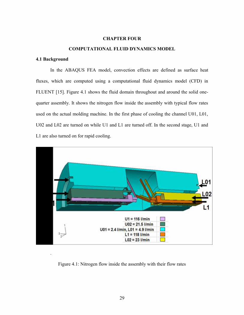
4.1 Background

In the ABAQUS FEA model, convection effects are defined as surface heat

fluxes, which are computed using a computational fluid dynamics model (CFD) in

FLUENT [15]. Figure 4.1 shows the fluid domain throughout and around the solid one-

quarter assembly. It shows the nitrogen flow inside the assembly with typical flow rates

used on the actual molding machine. In the first phase of cooling the channel U01, L01,

U02 and L02 are turned on while U1 and L1 are turned off. In the second stage, U1 and

L1 are also turned on for rapid cooling.

.

Figure 4.1: Nitrogen flow inside the assembly with their flow rates

30

During the first stage of cooling, U01 and L01 channels have very low nitrogen

flow rates in the order of 2-4 liters/minute where as the channels U02 and L02 have a

considerably greater flow rate, i.e., 20 liters/minute. Based on this information, it is

expected that most of the heat transfer takes place in the cooling channels. Therefore, this

research focuses on the CFD analysis of the fluid flow in a single cooling channel as

opposed to the whole fluid domain throughout and around the assembly. Another reason

for choosing this domain is due to the lack of computational power required to analyze

the whole fluid domain.

4.2 CFD Model of a Single Cooling Channel

4.2.1 Geometry of the Channel

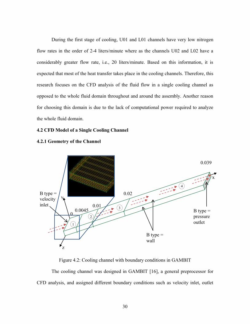
Figure 4.2: Cooling channel with boundary conditions in GAMBIT

The cooling channel was designed in GAMBIT [16], a general preprocessor for

CFD analysis, and assigned different boundary conditions such as velocity inlet, outlet

0.039

B type =

velocity

inlet

B type =

wall

B type = pressure

outlet

x

z

y 0.02

m

0.01

m 0

0.0045

m

3

4

1

2

31

pressure and wall, as shown in Figure 4.2. The cooling channel has a length of 0.039 m.

The channel is meshed with 20 nodes along the z direction (width) and 30 nodes along

the x direction (length) and with 10 nodes along the y direction (height). Meshing along

the width and height are shown in the zoomed view of the inlet section in Figure 4.3.

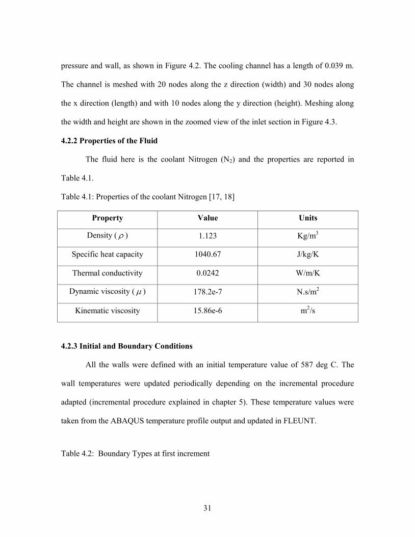
4.2.2 Properties of the Fluid

The fluid here is the coolant Nitrogen (N2) and the properties are reported in

Table 4.1.

Table 4.1: Properties of the coolant Nitrogen [17, 18]

Property Value Units

Density ( ) 1.123 Kg/m3

Specific heat capacity 1040.67 J/kg/K

Thermal conductivity 0.0242 W/m/K

Dynamic viscosity ( ) 178.2e-7 N.s/m2

Kinematic viscosity 15.86e-6 m2/s

4.2.3 Initial and Boundary Conditions

All the walls were defined with an initial temperature value of 587 deg C. The

wall temperatures were updated periodically depending on the incremental procedure

adapted (incremental procedure explained in chapter 5). These temperature values were

taken from the ABAQUS temperature profile output and updated in FLEUNT.

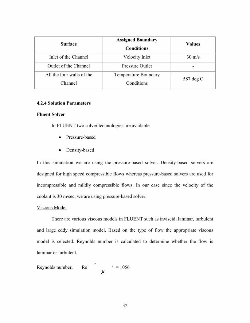
Table 4.2: Boundary Types at first increment

32

Surface Assigned Boundary

Conditions Values

Inlet of the Channel Velocity Inlet 30 m/s

Outlet of the Channel Pressure Outlet -

All the four walls of the

Channel

Temperature Boundary

Conditions 587 deg C

4.2.4 Solution Parameters

Fluent Solver

In FLUENT two solver technologies are available

Pressure-based

Density-based

In this simulation we are using the pressure-based solver. Density-based solvers are

designed for high speed compressible flows whereas pressure-based solvers are used for

incompressible and mildly compressible flows. In our case since the velocity of the

coolant is 30 m/sec, we are using pressure-based solver.

Viscous Model

There are various viscous models in FLUENT such as inviscid, laminar, turbulent

and large eddy simulation model. Based on the type of flow the appropriate viscous

model is selected. Reynolds number is calculated to determine whether the flow is

laminar or turbulent.

Reynolds number, * *

Re m hu D = 1056

33

where is the density, mu is the mean velocity,

hD is the hydraulic diameter and is

the dynamic viscosity of the nitrogen.

Hydraulic diameter, 2* *

( )h

H WD

H W = 5.5814 e-4 m

If the Reynolds number is less than 2300 we can consider it to be laminar flow [18].

Hence a laminar flow model is used.

In laminar flows, the fluid side heat transfer at walls is computed using Fourier's

law applied at the walls. FLUENT uses its discrete form:

( )f wallq k T n

where q is the heat flux, T is the temperature of the wall, n is the local coordinate normal

to the wall and kf is the thermal conductivity of the fluid.

4.2.5 Results

Figure 4.3 shows the heat flux distribution along the length of the channel when

the coolant nitrogen passes through the channel which is at a temperature of 587 deg C.

From the result above it can be inferred that most of the heat loss from the channel occurs

near the entrance of the channel. As the nitrogen flows along the length of the channel the

heat absorption is low and hence the heat flux is getting decreased.

34

Figure 4.3: Heat flux distribution along the length of the channel

Heat fluxes input into Abaqus are calculated for the partitions, shown in Figure

4.2, by calculating the surface average of Fluent results. The red curve in Figure 4.4

indicates the heat flux along the length of the channel. Figure 4.4 has 20 red curves and

each curve corresponds to different locations on the width of the channel as shown in

Figure 4.2 (20 nodes on the width) and are superimposed on the plot. The blue lines

indicate the nonlinear surface average of the heat fluxes along the length of the channel.

A MATLAB program was written to split the XY data for all these curves and calculate

the corresponding surface-averaged heat flux.

35

Figure 4.4: Heat flux along the channel length for channel

4.2.6 Analytical Validation

An approximate analytical calculation of the heat flux was done to verify the

average heat flux value given by FLUENT.

Length of the channel, L = 0.04 m

Width of the channel, W = 0.004 m

Height of the channel, H = 0.0003 m

Velocity, um = 30 m/sec

Nonlinear surface

average heat flux

Heat flux for each

node along the width

36

Hydraulic Diameter, Dh = 2*H*W/ (H+W)

= 5.5814e-4 m

Reynolds Number, Re = ( *mu *

hD ) /

= 1055.75

= 1056

Nusselt Number, Nu = (h*hD )/k

Nusselt Number and friction factor values are taken from Table 8.1 from reference [19]

using the cross section of the tube through which the fluid is flowing. Nusselt Number for

W/H = 13.33, Nu = 5.8126.

Assuming fully developed flow

Heat transfer coefficient, h = (k*Nu)/Dh

= 269.83 W/m2K

Heat Flux, Q = h*theta

= 269.73 * (860 – 300)

= 1.5105e5 W/m2

The heat flux value from the analytical calculation is estimated as 1.51e5 W/m2

compared to 1.85e5 W/m2 computed by Fluent. The difference in the values is due to

several approximations such as the Nusselt Number value.

4.3 CFD Model of the Entire Fluid Domain

4.3.1 Geometry

As explained earlier in the chapter the whole domain of the fluid is not considered

in this research study. However Benet Lab, a research partner in this project, considered

37

the whole fluid domain to calculate the heat fluxes. Figure 4.5 shows the model used by

Benet Lab for the heat flux calculation. The whole domain consists of around 60 surfaces

and for each surface the heat fluxes are calculated.

Figure 4.5: Model used by Benet Lab for heat flux calculation

4.3.2 Example Simulation Results

Few sample simulation results from FLUENT done by Benet Lab are shown

below. Figure 4.6 and 4.7 show the contour plot of the surface heat transfer coefficient

for the flow of nitrogen through the cooling and the streamlines throughout and around

the assembly, respectively.

38

Figure 4.6: Contour of surface heat transfer coefficient

Figure 4.7: Streamlines throughout and around the assembly

39

4.3.3 Design of Experiments

Benet Lab calculated the heat fluxes for all the surfaces using a Design Of

Experiments (DOE) approach, which allows a parametric representation of the heat

fluxes based on a limited sampling of the parametric space. DOE combines several

process variables in one study instead of creating a separate study for each variable.

Hence the amount of testing required will be drastically reduced and greater process

understanding will result [20]. The parameters considered while formulating DOE are

nitrogen flow rate in the channels, nitrogen temperature and the mold temperature. In this

research the heat fluxes defined on the surfaces other than the cooling channels, such as

outer surfaces of the die holders and cooling plates and other non-negligible surfaces are

taken from the data provided by the DOE results.

40

CHAPTER FIVE

COUPLING FEA AND CFD

5.1 Introduction

There are three general methods for solving the fluid-heat transfer problem. The

first method consists of solving the fluid flow problem and the transient heat transfer

analysis problem simultaneously using multi-physics software such as ANSYS [12]. The

complexity and size of the fluid domain prevents the use of this method given the

computational resources available. The second method consists of using the conjugate

heat transfer capability of Fluent, which can solve the heat transfer problem in the solid

domain in addition to the fluid flow problem. However, the solid domain is limited in

geometry and contact conductance values cannot be defined between solid faces. The

third method, used in this research, consists of decomposing the whole problem into the

fluid flow problem and the heat transfer problem and coordinating them in an incremental

procedure. This method allows a detailed definition of the solid domain with different

materials properties and surface conductance values at interfaces.

5.2 Interaction between FEA and CFD

This interaction study investigates the sensitivity of the solution to the frequency

of coupling or data exchange between the FEA and CFD solvers.

41

Figure 5.1: Schematic representation of the interaction between CFD and FEA

5.3 Coupled Solver for ABAQUS and FLUENT

In this study the heat fluxes are calculated first by Fluent and input into Abaqus at

the start of the transient heat transfer analysis. The wall temperatures computed by

Abaqus after a time increment T are used as input into Fluent. The heat fluxes are then

recalculated by Fluent and updated in ABAQUS for the next increment of the transient

heat transfer analysis. Each ABAQUS transient analysis is started from the temperature

field computed at the end of the previous increment (stored in ODB file). This interaction

between FLUENT and ABAQUS is repeated for every increment T. The number of

increments (defined by T) has an effect on the results. All these interactions are done

by a MATLAB code automatically. A parametric study has been done on how the delta t

affects the final simulation results.

CFD

Steady State fluid flow analysis

Input: Wall Temperatures

Output: Heat fluxes

FEA

Transient Heat transfer Analysis

Input: Heat fluxes

Output: Wall Temperatures

42

Figure 5.2: Schematic representation of the MATLAB code as a coupled solver between

FEA and CFD

Temperature Heat

flux

CAE

Input file

Finite

Element

Analysis

software

ABAQUS

FLUENT

case file

Computat

-ional

Fluid

Dynamics

software

FLUENT

MATLAB

code

43

Figure 5.3: Algorithmic representation of the interaction between CFD and FEA by

Matlab

t = 0

Stop the iteration

after 300 seconds

Run FLUENT for a steady state analysis of given wall temperature

Get Heat fluxes from FLUENT and update ABAQUS input file

Run ABAQUS for a transient heat transfer analysis from t to t+ t

seconds

Get the wall temperature values from ABAQUS results. Update

FLUENT input file.

If t >300

t = t+ t

No

Yes

44

5.4 Example Simulation Results

The following figures represent the temperature profile of the whole model at

different time intervals. This is the output of the simulation for a 30 increments

procedure, the data exchange between ABAQUS and FLUENT takes place for every 10

seconds (total simulation period is 300 seconds).

Figure 5.4: Simulation output, temperature distribution through the assembly at various

times of the cooling phase (a)At the starting (0th second), (b) At 10

th second and (c) At

300th second

(a) (b)

(c)

45

Figure 5.6 shows the temperature at the point where the thermocouple is placed in

the molding machine (shown in figure 3.4 in chapter 3), as a function of time for a 3

increment procedure (data coupled for every 100 seconds).

Figure 5.5: Temperature profile at the end of 300 seconds

46

CHAPTER 6

PARAMETRIC STUDIES

In this chapter various parametric studies are presented to understand the effect of

these parameters on the cooling rate. Forced convection by nitrogen in the cooling

channels alone does not account for the entire cooling taking place in the molding

machine. Radiation and as well as conduction are involved in the cooling phase (radiation

is explained in detail in section 3.5). Hence it is important to study their effect on the

cooling. In this study of the cooling phase there are two sets of unknown parameters:

a. Thermal contact conductance values, and

b. Radiation parameters (emissivity and ambient temperature).

These two sets were varied individually to match the experimental data.

6.1 Parametric Study on Contact Conductance Value ‘h’

In general, when two surfaces which are parallel and flat are pressed together,

they actually touch only at a limited number of discrete points. The contact is imperfect

and the real heat transfer area is only a small fraction of the apparent contact area [21]. H.

Yuncu did an experimental study of the thermal conductance of contact as a function of

apparent contact pressure. The author obtained data experimentally for steel, brass,

copper and aluminum test pieces having different surface roughness over a wide range of

contact pressures. The results obtained revealed good agreement of trend with theoretical

predictions, however numerical values vary widely. The values the author obtained for all

the test pieces were in the order of 1000 W/m2K.

47

CoCoE is an open source program that estimates the contact conductance, h,

between two surfaces under various conditions. CoCoE contains many empirical, lab-

tested credible data of different configurations of contact, collected from engineering

literature [22]. In CoCoE one has to input the contact materials, material in the gap,

surface roughness, temperature, and contact pressure. The program then extrapolates the

h value from the experimental and engineering literature database.

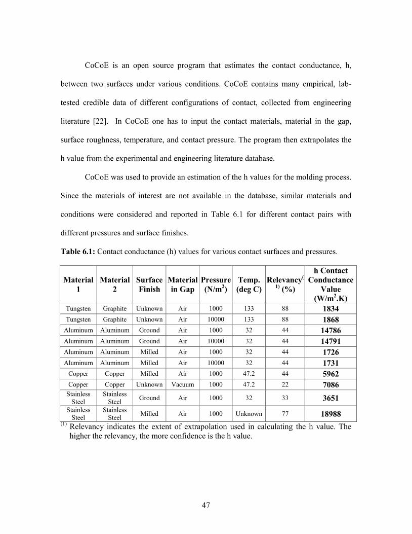
CoCoE was used to provide an estimation of the h values for the molding process.

Since the materials of interest are not available in the database, similar materials and

conditions were considered and reported in Table 6.1 for different contact pairs with

different pressures and surface finishes.

Table 6.1: Contact conductance (h) values for various contact surfaces and pressures.

Material

1

Material

2

Surface

Finish

Material

in Gap

Pressure

(N/m2)

Temp.

(deg C)

Relevancy(

1) (%)

h Contact

Conductance

Value

(W/m2.K)

Tungsten Graphite Unknown Air 1000 133 88 1834

Tungsten Graphite Unknown Air 10000 133 88 1868

Aluminum Aluminum Ground Air 1000 32 44 14786

Aluminum Aluminum Ground Air 10000 32 44 14791

Aluminum Aluminum Milled Air 1000 32 44 1726

Aluminum Aluminum Milled Air 10000 32 44 1731

Copper Copper Milled Air 1000 47.2 44 5962

Copper Copper Unknown Vacuum 1000 47.2 22 7086 Stainless

Steel

Stainless

Steel Ground Air 1000 32 33 3651

Stainless

Steel

Stainless

Steel Milled Air 1000 Unknown 77 18988

(1) Relevancy indicates the extent of extrapolation used in calculating the h value. The

higher the relevancy, the more confidence is the h value.

48

From this table we can infer the h values are in the order of thousands and the

values do not change very much when the pressure is increased by a factor of 10.

Materials used in the molding assembly such as silicon nitride, nickel binder,

cemented carbide are not available in the CoCoE database. However, all surfaces of the

assembly are very smooth (very low roughness), which will lead to large conductance

values. In terms of pressure, the fitting between parts is very tight and the pressure from

the compression during the molding process leads to large contact pressure between

surfaces. This will also result into large conductance values. From these considerations

and the CoCoE values shown in Table 6.1, the h values between all contact pairs in the

model are taken as 4500 W/m2K in all simulations in this research, except in the

parametric study presented in the next section.

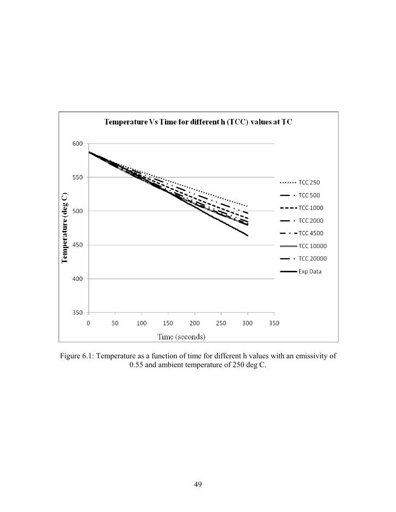
Figure 6.1 shows how the temperature varies with time at the location of the

thermocouple (which experimentally measures the temperature of the assembly) in the

mold dies with respect to different h values for a constant emissivity and ambient

temperature. The trend shows that as the h value increases between the contact pairs the

cooling rate increases.

49

Figure 6.1: Temperature as a function of time for different h values with an emissivity of 0.55 and ambient temperature of 250 deg C.

50

Figure 6.2: Temperature after 300 seconds of cooling at the location of the thermocouple

for different h values.

Also from the Figure 6.2, it is clear that when the h value is greater than 4500

W/m2K, the temperature remains almost the same. If the value is lower than the assumed

value then there may be difference between the predicted temperature and the actual

value. Since the h value is expected to be large due to the reasons stated in section 6.1 it

is assumed to take a higher value. As stated earlier h value of 4500 W/m2K was given for

all the contact pairs including the one between lens (glass) and tool. When compared to

all the contact pairs this interface might have a lower thermal contact of conductance,

however it is also given the same h value. It is due to the fact that this assumption might

affect the cooling of the lens alone, but the cooling of molding assembly as a whole.

51

6.2 Parametric Study on Emissivity and Ambient Temperature

A parametric study was done on the emissivity and the ambient temperature and

compared with the experimental data. Since the heaters surrounding the molding machine

are turned off during the cooling phase, the ambient (heaters) temperature was varied

between 200 and 300 deg C. Emissivity values of 0.55, 0.65 and 0.75 were considered for

three different ambient temperatures 200, 250 and 300 deg C. The following plots show

the temperature as a function of time at a point in the model where the thermocouple

(TC) was placed (shown in Chapter 3, figure 3.4).

Figure 6.3: Temperature as a function of time at Thermocouples with respect to various

emissivities for a constant ambient temperature of 200 deg C.

52

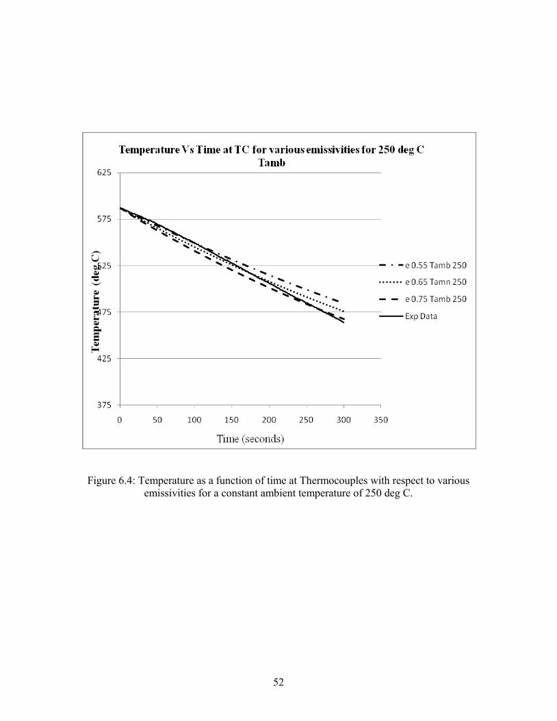
Figure 6.4: Temperature as a function of time at Thermocouples with respect to various

emissivities for a constant ambient temperature of 250 deg C.

53

Figure 6.5: Temperature as a function of time at Thermocouples with respect to various

emissivities for a constant ambient temperature of 300 deg C.

From the Figure 6.3 – 6.5 it is clear that as the emissivity increases the

temperature goes down whereas it is vice versa in the case of ambient temperature. It can

also be inferred that experimental data does not match for any of the values of emissivity

when the ambient temperature is 300 deg C.

The experimental data shows that the temperature at the thermocouples after the

300 second cooling period is 464 deg C. The table 6.2 summarizes the temperature at the

thermocouples for different combinations of emissivity and ambient temperature.

54

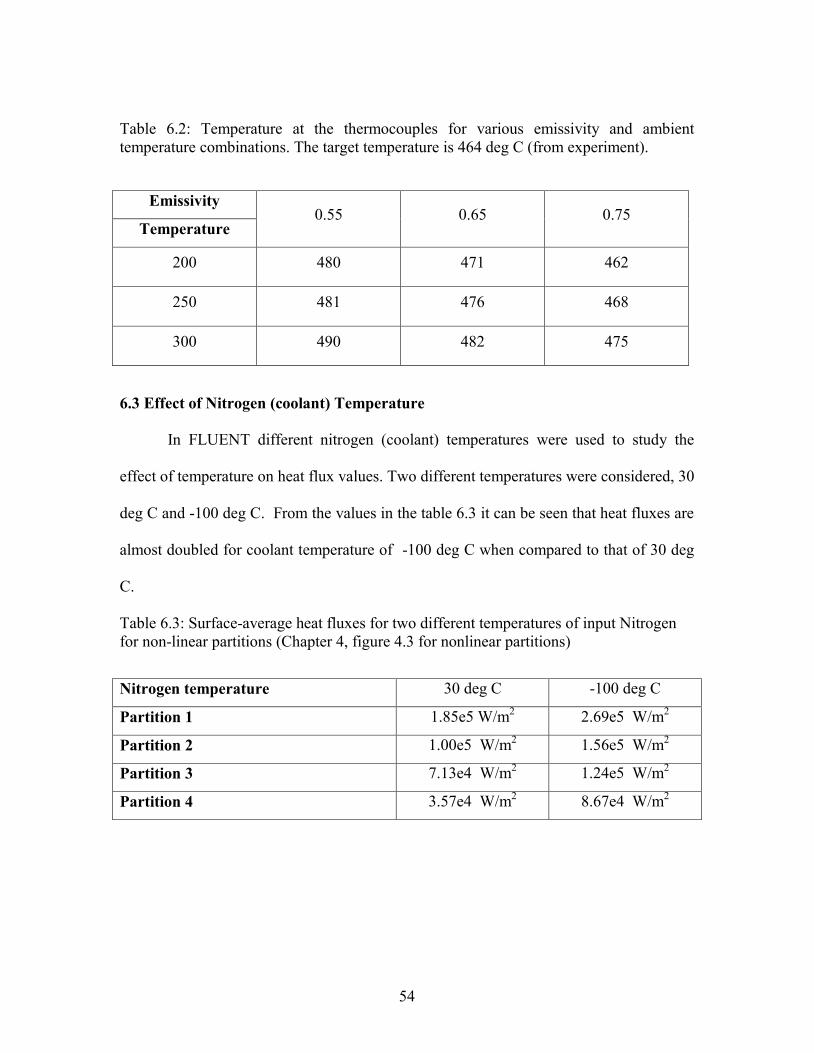
Table 6.2: Temperature at the thermocouples for various emissivity and ambient

temperature combinations. The target temperature is 464 deg C (from experiment).

Emissivity 0.55 0.65 0.75

Temperature

200 480 471 462

250 481 476 468

300 490 482 475

6.3 Effect of Nitrogen (coolant) Temperature

In FLUENT different nitrogen (coolant) temperatures were used to study the

effect of temperature on heat flux values. Two different temperatures were considered, 30

deg C and -100 deg C. From the values in the table 6.3 it can be seen that heat fluxes are

almost doubled for coolant temperature of -100 deg C when compared to that of 30 deg

C.

Table 6.3: Surface-average heat fluxes for two different temperatures of input Nitrogen

for non-linear partitions (Chapter 4, figure 4.3 for nonlinear partitions)

Nitrogen temperature 30 deg C -100 deg C

Partition 1 1.85e5 W/m2 2.69e5 W/m

2

Partition 2 1.00e5 W/m2 1.56e5 W/m2

Partition 3 7.13e4 W/m2 1.24e5 W/m2

Partition 4 3.57e4 W/m2 8.67e4 W/m

2

55

6.4 Parametric study on Number of Increments between FLUENT and ABAQUS

As explained in Chapter 5 a coupled solver for ABAQUS and FLUENT is written

using MATLAB. Figure 6.6 shows the temperature along the length of the cooling

channel for different incremental procedures. The trend here shows that as the number of

increments between the ABAQUS and FLUENT increases the temperature goes up along

the length of the channel. This is due to the fact that heat fluxes for a single-increment

procedure will be higher whereas the heat flux for a thirty-increment procedure will

decrease as the wall temperature gets updated at each increment and this results in

slightly lower heat fluxes and hence higher temperature.

Figure 6.6: Temperature along the length of the cooling channel for various incremental

procedures.

56

Figure 6.7 shows the value of heat fluxes that will be updated in the cooling

channels in ABAQUS for a five incremental procedure. For example, in the second

iteration, for 60 – 120 seconds interval of the total 300 seconds cooling period, a heat flux

of 1.32e5 W/m2 is applied to the first partition of the channel, 0 – 0.01 m. It can be

observed from the plot that the heat fluxes for a selected partition decreases in successive

iterations due to the reason that the temperature updated in FLUENT for successive

iterations reduce each time.

Figure 6.7: Heat flux along the length of the channel for the five increments in a five

incremental procedure.

57

Figure 6.8 shows the effect of the increments on the temperature at a point near

the entrance of the cooling channels with respect to time. A difference of 6.8 deg C is

observed at that point between a single increment and thirty incremental procedures.

Figure 6.8: Temperature at a point in the cooling channel for various incremental

procedures.

58

CHAPTER SEVEN

EXTRACTION OF BOUNDARY CONDITIONS

This chapter describes how the results obtained from the simulations performed in

this research can be used as boundary conditions for a parallel study, which is done using

a FEA 2D axisymmetric model of the molding process schematically represented in

Figure 7.1. In addition the heat flux output vectors through the whole model, tool and

lens are shown to discuss the validity of the axisymmetric assumption.

7.1 Transferring Data from the 3D Model to the 2D Axisymmetric Model

The red lines in Figure 7.1 indicate the boundary of the 2D axisymmetric model

used in the other study. One of the goals of this research is to determine whether the

axisymmetric assumption made in the 2D model is valid.

Figure 7.1: 3D model and boundary of the 2D axisymmetric model showing the upper

and lower tools and lens

Axis of

axisymmetry of

the 2D model

59

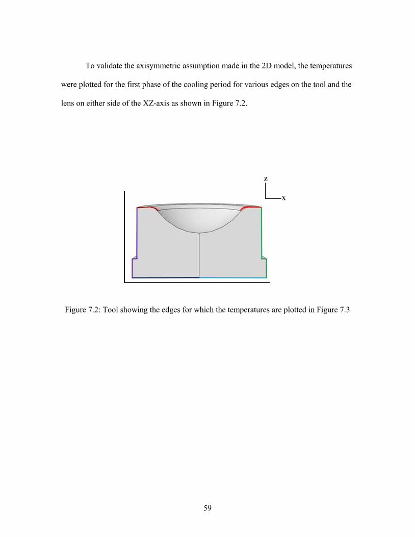
To validate the axisymmetric assumption made in the 2D model, the temperatures

were plotted for the first phase of the cooling period for various edges on the tool and the

lens on either side of the XZ-axis as shown in Figure 7.2.

Figure 7.2: Tool showing the edges for which the temperatures are plotted in Figure 7.3

X

Z

60

Figure 7.3: Temperature as a function of time for various edges in the tool shown in

Figure 7.2

From Figure 7.3 it is clear that the temperature plots follow the same trend on any

given edge. There is a maximum of 2.4 deg C difference in temperature between the left

and right sides. The temperature along the edges was calculated as an average of several

nodal temperatures along corresponding edges. The same conclusion can be drawn from

Figures 7.4 and 7.5 on the perpendicular section.

61

Figure 7.4: Tool and lens showing the edges in yz-plane for which the temperatures are

plotted in Figure 7.5

Figure 7.5: Temperature as a function of time for various edges in the tool and the lens shown in Figure 7.4

62

Figures 7.6 to 7.9 show various elements on the lens and tools and their

corresponding heat fluxes plotted for the 300 second cooling period.

Figure 7.6: Tool and lens showing the points where heat fluxes are plotted in Figure 7.7

Figure 7.7: Heat flux per area as a function of time for various elements in the tool and the lens shown in Figure 7.6

3

2

1

X

Z

Y

63

Figure 7.8: Tool and lens showing the points where heat fluxes are plotted in Figure.7.9

Figure 7.9: Heat flux per area as a function of time for various nodes (points) in the tool

and the lens shown in Figure 7.8

2 1

3

X

Z

Y

64

Figures 7.7 and 7.9 show that there is a significant difference in heat fluxes for the

elements on on different sides indicating that, since the heat fluxes are not axisymmetric,

they should not be used as boundary condition for the 2D axisymmetric model unless a

proper measure is considered.

7.2 Heat Flux Results throughout the Assembly

Figures 7.10 to 7-12 show the heat flux vectors in the whole molding machine

assembly. It can be seen that the heat flux vectors are more concentrated near the cooling

channels and the cooling plates than elsewhere in the model, stressing the fact that most

of the cooling takes place through the cooling channels.

Figure 7.10: Heat flux vector in the whole model

65

Figure 7.11: Heat flux vectors on a section on the xz-plane (a) after 10 seconds and (b)

after 300 seconds

Figure 7.12: Heat flux vectors on a section cut on a plane rotated 30 degrees about the z-

axis from the xz-plane (through the cooling channels) (a) after 10 seconds and (b) after

300 seconds

Figure 7.11 and 7.12 shows the heat flux vectors on a section cut on a xz-plane

and a section cut on the plane rotated 30 degrees about the z-axis from the xz-plane

(a) (b)

X

Z

Y

X

Z

Y (a) (b)

66

respectively at different time steps. It can be observed from the figures heat flux vectors

are more concentrated and oriented towards the cooling channels at the end of 300

seconds when compared to 10 seconds. Moreover the heat flux vectors on the outer

surface of the mold dies at the end of 10 seconds of cooling are more likely to be

horizontal indicating heat loss due to radiation is more during this period due to the

higher temperature difference between the molding assembly and the ambient

temperature, whereas at the end of 300 seconds, this difference is less and the heat flux

vectors are not horizontal.

Figure 7.13: Heat flux vectors for a section on a plane parallel to the yz-plane through the

middle of the lens (a) after 10 seconds (b) after 300 seconds

From Figure 7.3 it can be inferred that heat flux vectors at the end of the 300

seconds are higher than that of 10-second period.

Y

Z

(b) (a)

67

CHAPTER EIGHT

CONCLUSION AND FUTURE WORK

8.1 Conclusion

A 3D numerical model was developed to study and simulate the cooling phase of

the lens molding process. Various parametric studies were performed to study the effect

of several unknown and design parameters on the cooling rate. The assumption of

axisymmetry used in a 2D model of a parallel study is found to be relatively valid, since

there is only a small difference (i.e., 2.4 deg C) in temperature along the periphery of the

lens and tools during the first stage of cooling. From the 3D model developed in this

research, the temperature values can be provided as boundary conditions to the 2D

model. However, the heat fluxes vary significantly along the same boundary, which

should be considered if heat flux boundary conditions are used in the 2D model.

An iterative coupled procedure between the FEA and CFD models has been

successfully completed in MATLAB to take into account the effect of time-dependent

heat flux values during the cooling phase. Since the heat fluxes in the cooling channels

and temperature of the coolant are interdependent it is important to have such a coupling

between them. Moreover it is found that a five incremental procedure is sufficient for the

300-second cooling period. The MATLAB program is written in a generic form and can

be adapted to similar problems involving both solid and fluid interactions.

Thermal contact conductance values between surface pairs in contact in the model

have a significant effect on the cooling rate. In this research the TCC values between the

contact pairs are taken as 4500 W/m2K based on information available in the literature. It

68

is also inferred from the results that a higher value does not have a significant effect on

the cooling.

Radiation is taken into account by defining the emissivity of the material and the

ambient temperature. It is concluded that radiation also plays a significant role in the

cooling phase.

8.2 Future Work

i. In order to increase the fidelity of the model, accurate values of the contact

conductance at surface pairs should be determined. An experimental procedure

must be conducted to predict these values accurately for the specific materials of

the assembly under various contact pressures.

ii. In order to account for the potential pressure gradient in the radial direction of the

assembly, the 3D FEA model can be adapted to conduct a thermo-mechanical

analysis in ABAQUS to determine the stress distribution and a more accurate

temperature distribution through the lens and other parts of the molding machine.

iii. The model can be made more realistic by focusing on the radiation model. More

specifically, the heater coils and casing surrounding the assembly should be

included as part o the model and provide time-dependent ambient temperature

values. Note that the emissivity of the various materials would still be unknown

unless experimentally measured.

iv. Given more computational power, this numerical model can be used to simulate

all four stages of the lens molding process. A current simulation of the thermal

analysis with multiple CFD intermediate analyses runs for about one hour on a

69

single processor. A thermo-mechanical analysis would take several hours and

including the viscoelastic behavior of the glass material would certainly require

intensive parallel processing.

70

APPENDICES

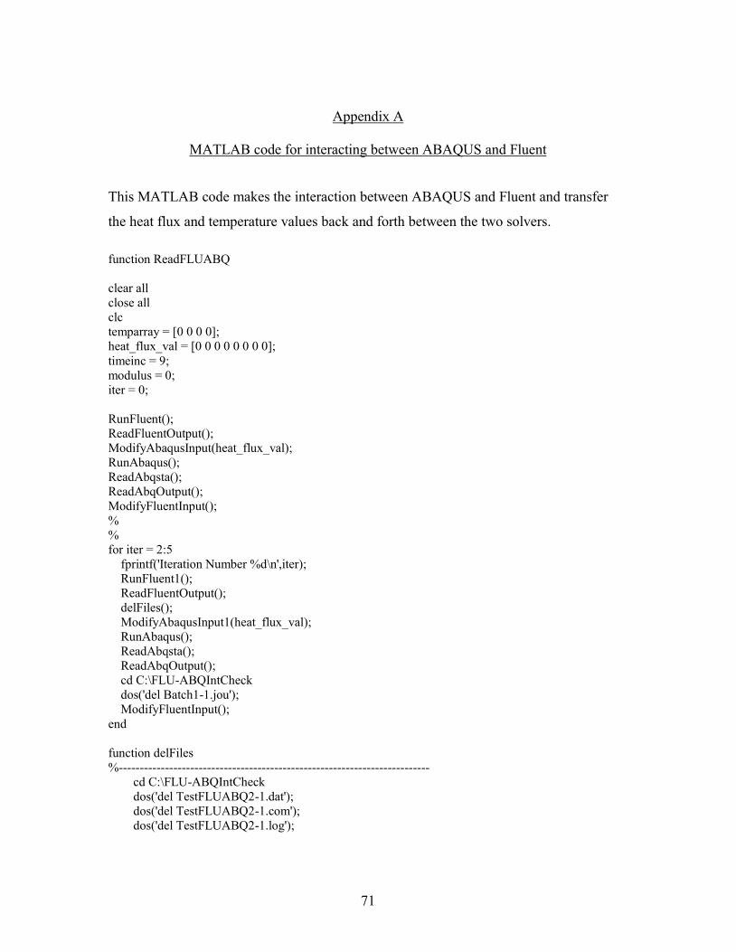
71

Appendix A

MATLAB code for interacting between ABAQUS and Fluent

This MATLAB code makes the interaction between ABAQUS and Fluent and transfer

the heat flux and temperature values back and forth between the two solvers.

function ReadFLUABQ

clear all

close all

clc

temparray = [0 0 0 0];

heat_flux_val = [0 0 0 0 0 0 0 0];

timeinc = 9;

modulus = 0;

iter = 0;

RunFluent();

ReadFluentOutput();

ModifyAbaqusInput(heat_flux_val);

RunAbaqus();

ReadAbqsta();

ReadAbqOutput();

ModifyFluentInput();

%

%

for iter = 2:5

fprintf('Iteration Number %d\n',iter);

RunFluent1();

ReadFluentOutput();

delFiles();

ModifyAbaqusInput1(heat_flux_val);

RunAbaqus();

ReadAbqsta();

ReadAbqOutput();

cd C:\FLU-ABQIntCheck

dos('del Batch1-1.jou');

ModifyFluentInput();

end

function delFiles

%--------------------------------------------------------------------------

cd C:\FLU-ABQIntCheck

dos('del TestFLUABQ2-1.dat');

dos('del TestFLUABQ2-1.com');

dos('del TestFLUABQ2-1.log');

72

dos('del TestFLUABQ2-1.sta');

dos('del TestFLUABQ2-1.msg');

dos('del TestFLUABQ2-1.inp');

str = 'copy TestFLUABQ2-1.odb Results';

str = strcat(str,num2str(iter),'.odb');

dos(str);

pause(5);

str = 'copy TestFLUABQ2-1.prt Results';

str = strcat(str,num2str(iter),'.prt');

dos(str);

% dos('copy TestFLUABQ2-1.prt Results.prt');

pause(5);

dos('del TestFLUABQ2-1.prt');

dos('del TestFLUABQ2-1.odb');

end

function RunFluent1

%--------------------------------------------------------------------------

% Change the Working Directory to run the FLUENT

cd C:\Fluent.Inc\ntbin\ntx86

% Dos command for executing the Batch file in FLUENT 3d

dos('fluent 3d -i "C:\FLU-ABQIntCheck\Batch1-1.jou"');

disp('FLUENT Job Started............');

pause(75);

disp('FLUENT Job Finished.');

fprintf('\n');

%Wait for 14 secs, so that the FLUENT job gets completed

end

%-----------------Function Implementations---------------------------------

%--------------------------------------------------------------------------

function RunFluent

%--------------------------------------------------------------------------

% Change the Working Directory to run the FLUENT

cd C:\Fluent.Inc\ntbin\ntx86

% Dos command for executing the Batch file in FLUENT 3d

dos('fluent 3d -i "C:\FLU-ABQIntCheck\Batch1.jou"');

disp('FLUENT Job Started............');

pause(20);

pause(75);

disp('FLUENT Job Finished.');

fprintf('\n');

%Wait for 14 secs, so that the FLUENT job gets completed

end

%--------------------------------------------------------------------------

function ReadFluentOutput

73

%--------------------------------------------------------------------------

% Changing the working directory to the path where the output file is

cd C:\Fluent.Inc\ntbin\ntx86

% Reading the Output (bot_1_wall.out) file generated by FLUENT

% to get the Heat Flux after 45 iterations

disp('Reading Fluent Output File....')

files = {'bot_1'; 'bot_2'; 'bot_3'; 'bot_4';'left_1';'left_2';'left_3';'left_4'};

heat_flux_val = [1;2;3;4;5;6;7;8];

for i = 1:1:8

fid = fopen([char(files(i)),'.out'],'r');

done = 0;

while ~done

tline = fgetl(fid);

if ~ischar(tline)

done = 1;

else

if ((strcmp(tline(1:3),'125')) ==1) % Number 125 denotes the last iteration

heat_flux_val(i) = abs(str2double(tline(4:length(tline))));

done=1;

end

end

end

fclose(fid);

end

fprintf('Fluent Output -- Heat Flux Value bot_1 = %d W/sq.m \n', heat_flux_val(1));

fprintf('Fluent Output -- Heat Flux Value bot_2 = %d W/sq.m \n', heat_flux_val(2));

fprintf('Fluent Output -- Heat Flux Value bot_3 = %d W/sq.m \n', heat_flux_val(3));

fprintf('Fluent Output -- Heat Flux Value bot_4 = %d W/sq.m \n', heat_flux_val(4));

fprintf('Fluent Output -- Heat Flux Value Left_1 = %d W/sq.m \n', heat_flux_val(5));

fprintf('Fluent Output -- Heat Flux Value Left_2 = %d W/sq.m \n', heat_flux_val(6));

fprintf('Fluent Output -- Heat Flux Value Left_3 = %d W/sq.m \n', heat_flux_val(7));

fprintf('Fluent Output -- Heat Flux Value Left_4 = %d W/sq.m \n', heat_flux_val(8));

end

%--------------------------------------------------------------------------

function ModifyAbaqusInput(heat_flux_val)

%--------------------------------------------------------------------------

cd C:\FLU-ABQIntCheck

%Reading the ABQ .inp file and changing the Dsflux value to the value

%obtained from the FLUENT monitor-2.out file

disp('Modifying ABQ .inp File....')

fid1 = fopen('TestFLUABQ2.inp','r'); % original file

fid2 = fopen('TestFLUABQ2-1.inp','w'); % new file

done = 0;

while ~done

tline = fgetl(fid1); % read each line

flag = 0;

if ~ischar(tline) % if "tline" is a number (ie, not a character), then reached the end of the

file

done = 1;

else

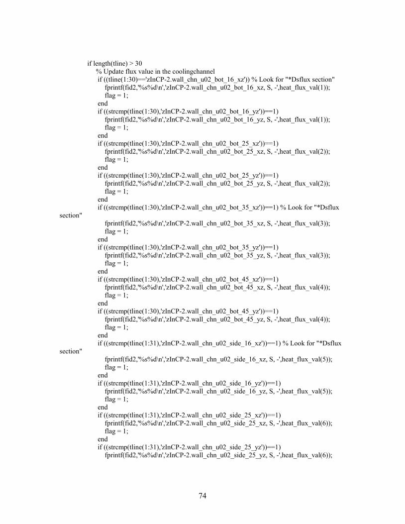
74

if length(tline) > 30

% Update flux value in the coolingchannel

if ((tline(1:30)=='zInCP-2.wall_chn_u02_bot_16_xz')) % Look for "*Dsflux section"

fprintf(fid2,'%s%d\n','zInCP-2.wall_chn_u02_bot_16_xz, S, -',heat_flux_val(1));

flag = 1;

end

if ((strcmp(tline(1:30),'zInCP-2.wall_chn_u02_bot_16_yz'))==1)

fprintf(fid2,'%s%d\n','zInCP-2.wall_chn_u02_bot_16_yz, S, -',heat_flux_val(1));

flag = 1;

end

if ((strcmp(tline(1:30),'zInCP-2.wall_chn_u02_bot_25_xz'))==1)

fprintf(fid2,'%s%d\n','zInCP-2.wall_chn_u02_bot_25_xz, S, -',heat_flux_val(2));

flag = 1;

end

if ((strcmp(tline(1:30),'zInCP-2.wall_chn_u02_bot_25_yz'))==1)

fprintf(fid2,'%s%d\n','zInCP-2.wall_chn_u02_bot_25_yz, S, -',heat_flux_val(2));

flag = 1;

end

if ((strcmp(tline(1:30),'zInCP-2.wall_chn_u02_bot_35_xz'))==1) % Look for "*Dsflux

section"

fprintf(fid2,'%s%d\n','zInCP-2.wall_chn_u02_bot_35_xz, S, -',heat_flux_val(3));

flag = 1;

end

if ((strcmp(tline(1:30),'zInCP-2.wall_chn_u02_bot_35_yz'))==1)

fprintf(fid2,'%s%d\n','zInCP-2.wall_chn_u02_bot_35_yz, S, -',heat_flux_val(3));

flag = 1;

end

if ((strcmp(tline(1:30),'zInCP-2.wall_chn_u02_bot_45_xz'))==1)

fprintf(fid2,'%s%d\n','zInCP-2.wall_chn_u02_bot_45_xz, S, -',heat_flux_val(4));

flag = 1;

end

if ((strcmp(tline(1:30),'zInCP-2.wall_chn_u02_bot_45_yz'))==1)

fprintf(fid2,'%s%d\n','zInCP-2.wall_chn_u02_bot_45_yz, S, -',heat_flux_val(4));

flag = 1;

end

if ((strcmp(tline(1:31),'zInCP-2.wall_chn_u02_side_16_xz'))==1) % Look for "*Dsflux

section"

fprintf(fid2,'%s%d\n','zInCP-2.wall_chn_u02_side_16_xz, S, -',heat_flux_val(5));

flag = 1;

end

if ((strcmp(tline(1:31),'zInCP-2.wall_chn_u02_side_16_yz'))==1)

fprintf(fid2,'%s%d\n','zInCP-2.wall_chn_u02_side_16_yz, S, -',heat_flux_val(5));

flag = 1;

end

if ((strcmp(tline(1:31),'zInCP-2.wall_chn_u02_side_25_xz'))==1)

fprintf(fid2,'%s%d\n','zInCP-2.wall_chn_u02_side_25_xz, S, -',heat_flux_val(6));

flag = 1;

end

if ((strcmp(tline(1:31),'zInCP-2.wall_chn_u02_side_25_yz'))==1)

fprintf(fid2,'%s%d\n','zInCP-2.wall_chn_u02_side_25_yz, S, -',heat_flux_val(6));

75

flag = 1;

end

if ((strcmp(tline(1:31),'zInCP-2.wall_chn_u02_side_35_xz'))==1) % Look for "*Dsflux

section"

fprintf(fid2,'%s%d\n','zInCP-2.wall_chn_u02_side_35_xz, S, -',heat_flux_val(7));

flag = 1;

end

if ((strcmp(tline(1:31),'zInCP-2.wall_chn_u02_side_35_yz'))==1)

fprintf(fid2,'%s%d\n','zInCP-2.wall_chn_u02_side_35_yz, S, -',heat_flux_val(7));

flag = 1;

end

if ((strcmp(tline(1:31),'zInCP-2.wall_chn_u02_side_45_xz'))==1)

fprintf(fid2,'%s%d\n','zInCP-2.wall_chn_u02_side_45_xz, S, -',heat_flux_val(8));

flag = 1;

end

if ((strcmp(tline(1:31),'zInCP-2.wall_chn_u02_side_45_yz'))==1)

fprintf(fid2,'%s%d\n','zInCP-2.wall_chn_u02_side_45_yz, S, -',heat_flux_val(8));

flag = 1;

end

if ((strcmp(tline(1:30),'zInDH-1.wall_chn_u02_top_16_xz'))==1)

fprintf(fid2,'%s%d\n','zInDH-1.wall_chn_u02_top_16_xz, S, -',heat_flux_val(1));

flag = 1;

end

if ((strcmp(tline(1:30),'zInDH-1.wall_chn_u02_top_16_yz'))==1)

fprintf(fid2,'%s%d\n','zInDH-1.wall_chn_u02_top_16_xz, S, -',heat_flux_val(1));

flag = 1;

end

if ((strcmp(tline(1:30),'zInDH-1.wall_chn_u02_top_25_xz'))==1)

fprintf(fid2,'%s%d\n','zInDH-1.wall_chn_u02_top_25_xz, S, -',heat_flux_val(2));

flag = 1;

end

if ((strcmp(tline(1:30),'zInDH-1.wall_chn_u02_top_25_yz'))==1)

fprintf(fid2,'%s%d\n','zInDH-1.wall_chn_u02_top_25_xz, S, -',heat_flux_val(2));

flag = 1;

end

if ((strcmp(tline(1:30),'zInDH-1.wall_chn_u02_top_35_xz'))==1)

fprintf(fid2,'%s%d\n','zInDH-1.wall_chn_u02_top_35_xz, S, -',heat_flux_val(3));

flag = 1;

end

if ((strcmp(tline(1:30),'zInDH-1.wall_chn_u02_top_35_yz'))==1)

fprintf(fid2,'%s%d\n','zInDH-1.wall_chn_u02_top_35_xz, S, -',heat_flux_val(3));

flag = 1;

end

if ((strcmp(tline(1:30),'zInDH-1.wall_chn_u02_top_45_xz'))==1)

fprintf(fid2,'%s%d\n','zInDH-1.wall_chn_u02_top_45_xz, S, -',heat_flux_val(4));

flag = 1;

end

if ((strcmp(tline(1:30),'zInDH-1.wall_chn_u02_top_45_yz'))==1)

fprintf(fid2,'%s%d\n','zInDH-1.wall_chn_u02_top_45_xz, S, -',heat_flux_val(4));

flag = 1;

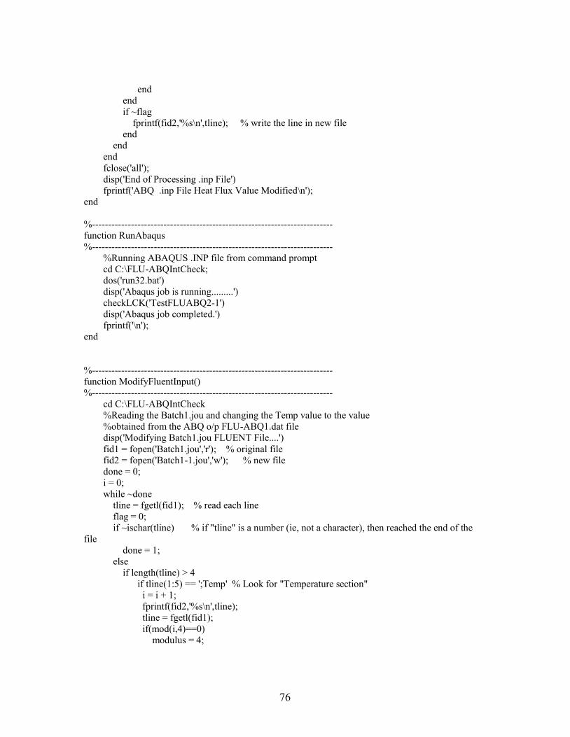
76

end

end

if ~flag

fprintf(fid2,'%s\n',tline); % write the line in new file

end

end

end

fclose('all');

disp('End of Processing .inp File')

fprintf('ABQ .inp File Heat Flux Value Modified\n');

end

%--------------------------------------------------------------------------

function RunAbaqus

%--------------------------------------------------------------------------

%Running ABAQUS .INP file from command prompt

cd C:\FLU-ABQIntCheck;

dos('run32.bat')

disp('Abaqus job is running.........')

checkLCK('TestFLUABQ2-1')

disp('Abaqus job completed.')

fprintf('\n');

end

%--------------------------------------------------------------------------

function ModifyFluentInput()

%--------------------------------------------------------------------------

cd C:\FLU-ABQIntCheck

%Reading the Batch1.jou and changing the Temp value to the value

%obtained from the ABQ o/p FLU-ABQ1.dat file

disp('Modifying Batch1.jou FLUENT File....')

fid1 = fopen('Batch1.jou','r'); % original file

fid2 = fopen('Batch1-1.jou','w'); % new file

done = 0;

i = 0;

while ~done

tline = fgetl(fid1); % read each line

flag = 0;

if ~ischar(tline) % if "tline" is a number (ie, not a character), then reached the end of the

file

done = 1;

else

if length(tline) > 4

if tline(1:5) == ';Temp' % Look for "Temperature section"

i = i + 1;

fprintf(fid2,'%s\n',tline);

tline = fgetl(fid1);

if(mod(i,4)==0)

modulus = 4;

77

else

modulus = mod(i,4);

end

fprintf(fid2,'%d\n',(temparray(modulus)+273)); % Update temp value in the

coolingchannel

flag = 1;

end

end

if ~flag

fprintf(fid2,'%s\n',tline); % write the line in new file

end

end

end

fclose('all');

disp('End of Modifying .jou File')

fprintf('\n');

end

%--------------------------------------------------------------------------

function checkLCK(filename)

%--------------------------------------------------------------------------

done = 0;

flag = 0;

while ~done

lck = dir([filename,'.lck']);

if flag == 0

if ~isempty(lck) % lck file was created

flag = 1;

end

else

if isempty(lck) % lck file was removed

done = 1;

disp('lck removed')

end

end

pause(2)

end

end

function ReadAbqsta

%--------------------------------------------------------------------------

cd C:\FLU-ABQIntCheck

fid = fopen('TestFLUABQ2-1.sta','r');

done = 0;

disp('Processing STA to find Inc Number....')

while ~done

tline = fgetl(fid);

if ~ischar(tline)

done = 1;

else

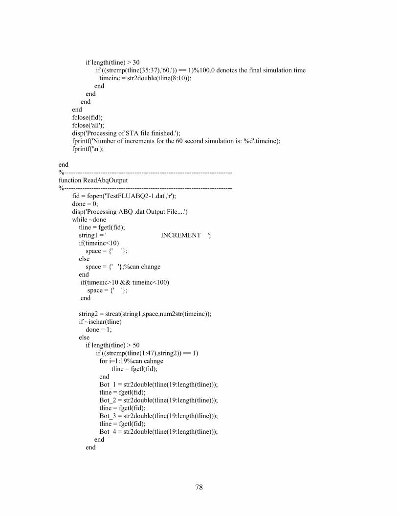
78

if length(tline) > 30

if ((strcmp(tline(35:37),'60.')) == 1)%100.0 denotes the final simulation time

timeinc = str2double(tline(8:10));

end

end

end

end

fclose(fid);

fclose('all');

disp('Processing of STA file finished.');

fprintf('Number of increments for the 60 second simulation is: %d',timeinc);

fprintf('\n');

end

%--------------------------------------------------------------------------

function ReadAbqOutput

%--------------------------------------------------------------------------

fid = fopen('TestFLUABQ2-1.dat','r');

done = 0;

disp('Processing ABQ .dat Output File....')

while ~done

tline = fgetl(fid);

string1 = ' INCREMENT ';

if(timeinc<10)

space = {' '};

else

space = {' '};%can change

end

if(timeinc>10 && timeinc<100)

space = {' '};

end

string2 = strcat(string1,space,num2str(timeinc));

if ~ischar(tline)

done = 1;

else

if length(tline) > 50

if ((strcmp(tline(1:47),string2)) == 1)

for i=1:19%can cahnge

tline = fgetl(fid);

end

Bot_1 = str2double(tline(19:length(tline)));

tline = fgetl(fid);

Bot_2 = str2double(tline(19:length(tline)));

tline = fgetl(fid);

Bot_3 = str2double(tline(19:length(tline)));

tline = fgetl(fid);

Bot_4 = str2double(tline(19:length(tline)));

end

end

79

end

end

fclose(fid);

fclose('all');

temparray = [Bot_1 Bot_2 Bot_3 Bot_4];

disp('Processing of .DAT file finished.');

fprintf('Temp value for the first partition is: %d K', Bot_1);

fprintf('Temp value for the secon partition is: %d K', Bot_2);

fprintf('Temp value for the third partition is: %d K', Bot_3);

fprintf('Temp value for the fourt partition is: %d K', Bot_4);

fprintf('\n');

end

%--------------------------------------------------------------------------

function ModifyAbaqusInput1(heat_flux_val)

%--------------------------------------------------------------------------

cd C:\FLU-ABQIntCheck

%Reading the ABQ .inp file and changing the Dsflux value to the value

%obtained from the FLUENT monitor-2.out file

disp('Modifying ABQ.inp File....')

fid1 = fopen('TestFLUABQ2.inp','r'); % original file

fid2 = fopen('TestFLUABQ2-1.inp','w'); % new file

done = 0;

while ~done

tline = fgetl(fid1); % read each line

flag = 0;

if ~ischar(tline) % if "tline" is a number (ie, not a character), then reached the end of the

file

done = 1;

else

if length(tline) > 12

if (tline(1:10) == '** Name: P')%checking for Predefined Field Definition

fprintf(fid2,'%s\n',tline);

tline = fgetl(fid1);

% Update flux value in the coolingchannel

str = '*Initial Conditions, type=TEMPERATURE, file=C:/FLU-

ABQIntCheck/Results';

str = strcat(str,num2str(iter),'.odb, step=1, inc=');

fprintf(fid2,'%s%s\n',str,num2str(timeinc));

% fprintf(fid2,'%s%s\n','*Initial Conditions, type=TEMPERATURE, file=C:/FLU-

ABQIntCheck/Results.odb, step=1, inc=',num2str(timeinc));

flag = 1;

end

if tline(1:13) == '_PickedSet211'% Do not write this line

flag = 1;

end

end

if length(tline) > 30

% Update flux value in the coolingchannel

if ((tline(1:30)=='zInCP-2.wall_chn_u02_bot_16_xz')) % Look for "*Dsflux section"

80

fprintf(fid2,'%s%d\n','zInCP-2.wall_chn_u02_bot_16_xz, S, -',heat_flux_val(1));

flag = 1;

end

if ((strcmp(tline(1:30),'zInCP-2.wall_chn_u02_bot_16_yz'))==1)

fprintf(fid2,'%s%d\n','zInCP-2.wall_chn_u02_bot_16_yz, S, -',heat_flux_val(1));

flag = 1;

end

if ((strcmp(tline(1:30),'zInCP-2.wall_chn_u02_bot_25_xz'))==1)

fprintf(fid2,'%s%d\n','zInCP-2.wall_chn_u02_bot_25_xz, S, -',heat_flux_val(2));

flag = 1;

end

if ((strcmp(tline(1:30),'zInCP-2.wall_chn_u02_bot_25_yz'))==1)

fprintf(fid2,'%s%d\n','zInCP-2.wall_chn_u02_bot_25_yz, S, -',heat_flux_val(2));

flag = 1;

end

if ((strcmp(tline(1:30),'zInCP-2.wall_chn_u02_bot_35_xz'))==1) % Look for "*Dsflux

section"

fprintf(fid2,'%s%d\n','zInCP-2.wall_chn_u02_bot_35_xz, S, -',heat_flux_val(3));

flag = 1;

end

if ((strcmp(tline(1:30),'zInCP-2.wall_chn_u02_bot_35_yz'))==1)

fprintf(fid2,'%s%d\n','zInCP-2.wall_chn_u02_bot_35_yz, S, -',heat_flux_val(3));

flag = 1;

end

if ((strcmp(tline(1:30),'zInCP-2.wall_chn_u02_bot_45_xz'))==1)

fprintf(fid2,'%s%d\n','zInCP-2.wall_chn_u02_bot_45_xz, S, -',heat_flux_val(4));

flag = 1;

end

if ((strcmp(tline(1:30),'zInCP-2.wall_chn_u02_bot_45_yz'))==1)

fprintf(fid2,'%s%d\n','zInCP-2.wall_chn_u02_bot_45_yz, S, -',heat_flux_val(4));

flag = 1;

end

if ((strcmp(tline(1:31),'zInCP-2.wall_chn_u02_side_16_xz'))==1) % Look for "*Dsflux

section"

fprintf(fid2,'%s%d\n','zInCP-2.wall_chn_u02_side_16_xz, S, -',heat_flux_val(5));

flag = 1;

end

if ((strcmp(tline(1:31),'zInCP-2.wall_chn_u02_side_16_yz'))==1)

fprintf(fid2,'%s%d\n','zInCP-2.wall_chn_u02_side_16_yz, S, -',heat_flux_val(5));

flag = 1;

end

if ((strcmp(tline(1:31),'zInCP-2.wall_chn_u02_side_25_xz'))==1)

fprintf(fid2,'%s%d\n','zInCP-2.wall_chn_u02_side_25_xz, S, -',heat_flux_val(6));

flag = 1;

end

if ((strcmp(tline(1:31),'zInCP-2.wall_chn_u02_side_25_yz'))==1)

fprintf(fid2,'%s%d\n','zInCP-2.wall_chn_u02_side_25_yz, S, -',heat_flux_val(6));

flag = 1;

end

81

if ((strcmp(tline(1:31),'zInCP-2.wall_chn_u02_side_35_xz'))==1) % Look for "*Dsflux

section"

fprintf(fid2,'%s%d\n','zInCP-2.wall_chn_u02_side_35_xz, S, -',heat_flux_val(7));

flag = 1;

end

if ((strcmp(tline(1:31),'zInCP-2.wall_chn_u02_side_35_yz'))==1)

fprintf(fid2,'%s%d\n','zInCP-2.wall_chn_u02_side_35_yz, S, -',heat_flux_val(7));

flag = 1;

end

if ((strcmp(tline(1:31),'zInCP-2.wall_chn_u02_side_45_xz'))==1)

fprintf(fid2,'%s%d\n','zInCP-2.wall_chn_u02_side_45_xz, S, -',heat_flux_val(8));

flag = 1;

end

if ((strcmp(tline(1:31),'zInCP-2.wall_chn_u02_side_45_yz'))==1)

fprintf(fid2,'%s%d\n','zInCP-2.wall_chn_u02_side_45_yz, S, -',heat_flux_val(8));

flag = 1;

end

if ((strcmp(tline(1:30),'zInDH-1.wall_chn_u02_top_16_xz'))==1)

fprintf(fid2,'%s%d\n','zInDH-1.wall_chn_u02_top_16_xz, S, -',heat_flux_val(1));

flag = 1;

end

if ((strcmp(tline(1:30),'zInDH-1.wall_chn_u02_top_16_yz'))==1)

fprintf(fid2,'%s%d\n','zInDH-1.wall_chn_u02_top_16_xz, S, -',heat_flux_val(1));

flag = 1;

end

if ((strcmp(tline(1:30),'zInDH-1.wall_chn_u02_top_25_xz'))==1)

fprintf(fid2,'%s%d\n','zInDH-1.wall_chn_u02_top_25_xz, S, -',heat_flux_val(2));

flag = 1;

end

if ((strcmp(tline(1:30),'zInDH-1.wall_chn_u02_top_25_yz'))==1)

fprintf(fid2,'%s%d\n','zInDH-1.wall_chn_u02_top_25_xz, S, -',heat_flux_val(2));

flag = 1;

end

if ((strcmp(tline(1:30),'zInDH-1.wall_chn_u02_top_35_xz'))==1)

fprintf(fid2,'%s%d\n','zInDH-1.wall_chn_u02_top_35_xz, S, -',heat_flux_val(3));

flag = 1;

end

if ((strcmp(tline(1:30),'zInDH-1.wall_chn_u02_top_35_yz'))==1)

fprintf(fid2,'%s%d\n','zInDH-1.wall_chn_u02_top_35_xz, S, -',heat_flux_val(3));

flag = 1;

end

if ((strcmp(tline(1:30),'zInDH-1.wall_chn_u02_top_45_xz'))==1)

fprintf(fid2,'%s%d\n','zInDH-1.wall_chn_u02_top_45_xz, S, -',heat_flux_val(4));

flag = 1;

end

if ((strcmp(tline(1:30),'zInDH-1.wall_chn_u02_top_45_yz'))==1)

fprintf(fid2,'%s%d\n','zInDH-1.wall_chn_u02_top_45_xz, S, -',heat_flux_val(4));

flag = 1;

end

end

82

if ~flag

fprintf(fid2,'%s\n',tline); % write the line in new file

end

end

end

fclose('all');

disp('End of Processing .inp File')

fprintf('ABQ.inp File Heat Value Modified\n');

end

end

83

REFERENCES

[1] B. Ananthasayanam, “Computational modeling of precision molding of aspheric glass

optics,” PhD Dissertation, Clemson University, 2008.

[2] J.Yana, T.Zhoua, J.Masudab, T.Kuriyagawaa, “Modeling high-temperature glass

molding process by coupling heat transfer and viscous deformation analysis,” Precision Engineering, Vol. 33, pp. 150–159, 2009.

[3] A.G. Smitha, L.C. Wrobela, B.A. McCallab, P.S. Allanb, P.R. Hornsbyc, “A

computational model for the cooling phase of injection moulding,” Journal of materials

processing technology, Vol. 195, pp. 305–313, 2008.

[4] L. Sridhar and K. A. Narh, “The effect of temperature dependent thermal properties

on process parameter prediction in injection molding,” Int. Comm. Heat Mass Transfer,

Vol. 27, No. 3, pp. 325-332, 2000.

[5] E. Bilgen, “Conjugate heat transfer by conduction and natural convection on a heated vertical wall,” Applied Thermal Engineering, Vol. 29, pp. 334–339, 2009.

[6] H. Zhou, D. Li, “Three-Dimensional Numerical Simulation of the Pressing Process in

TV Panel Production,” Simulation Modeling Practice and Theory, Vol. 13, pp. 273–285,

2005.

[7] L. Lanoye, J. Vierendeels, P. Segers and P. Verdonck, “Vascular fluid-structure

interaction using Fluent and Abaqus software,” Journal of Biomechanics, Vol. 39, Supplement 1, pp. S440, 2006.

[8] Y. Lin, H. Li, S. Chen, C. Shen, “3D numerical simulation of transient temperature

field for lens mold embedded with heaters,” Int. Comm. Heat Mass Transfer, Vol. 32,

No. 3, pp. 1221-1230, 2005.

[9] X. F. Peng, B. X. Wang, G. P. Peterson and H. B. Ma, “Experimental investigation of

heat transfer in flat plates with rectangular micro channels,” International journal of heat and mass transfer, Vol. 38, No. 1, pp. 127-137, 1995.

[10] H.L. Mo, Y.X. Zhou, T.Y. Zhu, T.W. Guo, “Forced convection of low temperature nitrogen gas in rectangular channels with small aspect ratio,” Cryogenics, Vol. 44, pp.

301-307, 2004.

[11] http://www.simulia.com/products/abaqus_cae.html

[12] http://www.ansys.com/

84

[13] C.V. Madhusudana, Thermal Contact Conductance, Springer, Berlin. ISBN 0-387-

94534-2 (1996).

[14] Thermal Contact Conductance - NASA Technical Memorandum 110429

[15] http://www.fluent.com/

[16] http://www.fluent.com/software/gambit/new_features_24.htm

[17] Fluent 6.0 User Guide. Fluent Inc., 2003.

[18] Bruce R. Munson, Donald F. Young, Theodore H. Okiishi, Fundamentals of Fluid

Mechanics, 4thEd. Wiley, 2002.

[19] F. P. Incropera, D. P. Dewitt, T. L. Bergman, A. S. Lavine, Fundamentals of Heat

and Mass Transfer, 6thEd, Wiley, 2002.

[20] Larry B. Barrentine, An Introduction to Design of Experiments: A Simplified Approach, ASQ Quality Press, 1999.

[21] H. Yuncuu, “Thermal contact conductance of nominally flat surfaces,” Heat Mass Transfer, Vol. 43, pp. 1-5, 2006.

[22] http://cocoe.sourceforge.net/