modeling the impacts of john day ... - cbr.washington.edu
TRANSCRIPT
1
Modeling the impacts of John Day drawdown on the survival of salmonid stocks
James J. Anderson and Richard W. Zabel
Columbia Basin Research
University of Washington
Box 358218
Seattle, WA 98195
Richard A. Hinrichsen
Hinrichsen Fisheries Consulting
Lakeview Medical Dental Building
3216 NE 45th Pl Suite 303W
Seattle WA 98105
January 12, 2000
2
CONTENTS
1 INTRODUCTION ...............................................................................................................................................7
2 ACTIONS.............................................................................................................................................................8
3 MEASURES OF FISH PERFORMANCE......................................................................................................10
3.1 SURVIVAL STANDARD: 24-YEAR ..................................................................................................................103.2 RECOVERY STANDARD: 48-YEAR .................................................................................................................103.3 EQUILIBRIUM SPAWNERS ..............................................................................................................................113.4 SMOLT PASSAGE MEASURES ........................................................................................................................11
4 LIFE-CYCLE FRAMEWORK ........................................................................................................................11
4.1 FRESHWATER PRODUCTION (P).....................................................................................................................134.1.1 Density dependence parameter (b) ......................................................................................................134.1.2 Stock equilibrium numbers ..................................................................................................................14
4.2 PASSAGE SURVIVAL (SM)..............................................................................................................................154.2.1 In-river survival (Vn) ...........................................................................................................................154.2.2 Natural River Drawdown survival (Vd )..............................................................................................174.2.3 Spill Crest and Food Control Drawdown survival (Vd) ......................................................................18
4.3 OCEAN/ESTUARY SURVIVAL (SO) .................................................................................................................204.3.1 Extra mortality.....................................................................................................................................214.3.2 Delayed mortality ................................................................................................................................23
4.4 ADULT UPSTREAM MIGRATION SURVIVAL (SA) .............................................................................................25
5 BAYESIAN LIFE-CYCLE ANALYSIS ..........................................................................................................26
5.1 ACTIONS EVALUATED FOR SPRING AND FALL CHINOOK.................................................................................275.2 HYPOTHESES ................................................................................................................................................27
5.2.1 Spring chinook hypotheses ..................................................................................................................285.2.2 Hypotheses Evaluated for Fall Chinook ..............................................................................................295.2.3 Weighting hypotheses ..........................................................................................................................31
5.3 BSM RESULTS..............................................................................................................................................325.3.1 Probability of Survival and Recovery ..................................................................................................325.3.2 Relative risks........................................................................................................................................34Equilibrium stock levels.......................................................................................................................................36
6 DETERMINISTIC LIFE-CYCLE ANALYSIS ..............................................................................................40
6.1 DETERMINISTIC LIFE STAGE PARAMETERS ...................................................................................................446.2 EQUATIONS FOR COMPARISON OF ACTIONS ...................................................................................................47
6.2.1 Equilibrium Population and MSY Differences in Drawdown Actions................................................476.2.2 Equilibrium and MSY Differences of Transport vs. Drawdown Actions .............................................476.2.3 Equivalence points...............................................................................................................................48
6.3 RESULTS.......................................................................................................................................................496.3.1 Pairwise comparison of drawdown alternatives..................................................................................496.3.2 Pairwise comparison of transport vs. drawdown alternatives.............................................................52
7 DOWNSTREAM PASSAGE MODEL ............................................................................................................59
7.1 CONFIGURATION FOR JOHN DAY DRAWDOWN ..............................................................................................597.2 PASSAGE MODEL RESULTS ...........................................................................................................................60
7.2.1 Mortality associated with the John Day project ..................................................................................607.2.2 Changes in travel time under John Day operations ............................................................................617.2.3 Spring Chinook Results........................................................................................................................617.2.4 Fall Chinook results.............................................................................................................................63
3
8 DISCUSSION.....................................................................................................................................................65
8.1 BAYESIAN ANALYSIS ....................................................................................................................................678.2 DETERMINISTIC LIFE-CYCLE ANALYSIS .........................................................................................................698.3 SMOLT PASSAGE ANALYSIS ...........................................................................................................................708.4 SUMMARY ....................................................................................................................................................718.5 FINAL REMARKS...........................................................................................................................................75
9 REFERENCES ..................................................................................................................................................76
10 COMMENTS BY PATH AND RESPONSES .............................................................................................78
10.1 COMMENTS PROVIDED BY PAUL WILSON OF CBWFW ARE INCLUDED BELOW.............................................7810.2 RESPONSE TO REVIEW...................................................................................................................................80
List of FiguresFIGURE 1. LIFE CYCLE OF SALMON EXTENDING FROM FRESHWATER PRODUCTION STAGE, P, TO HYDROSYSTEM
SURVIVAL, SM, FROM LOWER GRANITE DAM (LGR) TO BONNEVILLE DAM (BON), WHICH INCLUDES IN RIVERAND TRANSPORT PASSAGE, TO OCEAN SURVIVAL, SO, TO UPRIVER ADULT MIGRATION SURVIVAL, SA. S SPAWNERSPRODUCE R RECRUITS. .........................................................................................................................................12
FIGURE 2. RESERVOIR WITH FREE-FLOWING AND IMPOUNDED PORTIONS. THE TERMS ARE RESERVOIR ELEVATION E,LENGTH L, VOLUME V(E), FLOW F, AND STREAM VELOCITY UFREE.....................................................................18
List of TablesTABLE 1. ALTERNATIVE ACTIONS EVALUATED ...............................................................................................................9TABLE 2: RICKER COEFFICIENTS FOR SPRING AND FALL CHINOOK FROM THE COLUMBIA/SNAKE RIVER SYSTEM STOCKS.
SPAWNERS WERE ON REDDS AND RECRUITS WERE ESTIMATED TO MOUTH OF COLUMBIA RIVER. THE SNAKERIVER SPRING CHINOOK ESTIMATES ARE THE MEAN VALUES OF 7 INDEX STOCKS. ................................................14
TABLE 3. DRAWDOWN SURVIVALS VD THROUGH FREE-FLOWING REACHES OF THE SNAKE RIVER AND JOHN DAYRESERVOIR. ..........................................................................................................................................................17
TABLE 4: WATER VELOCITIES (MILES/DAY) FOR DIFFERENT FLOWS AND POOL ELEVATIONS.........................................19TABLE 5: CHARACTERISTIC OCEAN SURVIVAL FACTOR �N, AS DETERMINED BY EXTRA MORTALITY, UNDER DIFFERENT
PASSAGE MODEL HYPOTHESES USING THE DELTA MODEL DEVELOPED IN PATH (HINRICHSEN AND PAULSEN1998) WITH RANGES (MIN-MAX). SPRING �N ESTIMATES FROM REGRESSIONS OF VN VS. �N WITH VN = 0.2 FOR1975-1990 AND VN = 0.4 FOR 1952-1990 PERIOD. FALL CHINOOK ESTIMATES FROM SPAWNER/RECRUITANALYSIS (PETERS ET AL. 1999)...........................................................................................................................23
TABLE 6: SPRING CHINOOK GEOMETRIC AVERAGE ESTIMATES OF D FOR EARLY EXPERIMENTAL PERIOD (PRE-1980)AND CURRENT/PROSPECTIVE PERIOD (POST-1980). ...............................................................................................24
TABLE 7: FIVE FALL CHINOOK HYPOTHESES OF D FOR THE EXISTING OPERATIONS (RETROSPECTIVE) FUTURE PERIOD(PROSPECTIVE). ....................................................................................................................................................25
TABLE 8: CONVERSION RATE OF ADULT MIGRATION SURVIVAL (SA) FROM BONNEVILLE DAM TAILRACE TO THESPAWNING GROUNDS (MARMOREK ET AL. 1996, PETERS ET AL. 1999). ...............................................................26
TABLE 9: ACTIONS EVALUATED WITH THE PATH BAYESIAN MODEL...........................................................................27TABLE 10: PATH HYPOTHESES FOR SPRING CHINOOK ANALYSIS.................................................................................29TABLE 11: HYPOTHESES USED IN THE FALL CHINOOK ANALYSIS...................................................................................30TABLE 12: NUMBER OF HYPOTHESES UNDER EACH ACTION .........................................................................................31TABLE 13: SPRING CHINOOK 24-YEAR SURVIVAL PROBABILITY MEAN VALUES. ...........................................................32TABLE 14: SPRING CHINOOK 48-YEAR RECOVERY PROBABILITY MEAN VALUES. ..........................................................33TABLE 15: FALL CHINOOK PROBABILITY OF MEETING A 24-YEAR SURVIVAL STANDARD. .............................................33TABLE 16: FALL CHINOOK PROBABILITY OF MEETING THE 48-YR RECOVER STANDARD................................................34TABLE 17: RELATIVE RISK FOR SPRING CHINOOK. B1-A3 IS GAIN IN PROBABILITY OF MEETING STANDARD DUE TO
TAKING ACTION B1 OVER ACTION A3. A3-A1 IS GAIN IN PROBABILITY OF MEETING STANDARD DUE TO TAKINGACTION A3 OVER ACTION A1................................................................................................................................35

4
TABLE 18: RELATIVE RISK FOR FALL CHINOOK. B1-A3 IS GAIN IN PROBABILITY OF MEETING STANDARD DUE TO TAKINGACTION B1 OVER ACTION A3. A3-A2 IS GAIN IN PROBABILITY OF MEETING STANDARD DUE TO TAKING ACTION A3OVER ACTION A2..................................................................................................................................................36
TABLE 19: SPRING CHINOOK EQUILIBRIUM STOCK LEVELS FOR THE INDEX SNAKE RIVER ESU STOCKS UNDERDIFFERENT ACTIONS AND HYPOTHESES WEIGHTINGS. B1- A3 AND A3- A1 ARE THE RELATIVE GAINS IN NUMBERSOF SPAWNERS BETWEEN TWO ACTIONS. ................................................................................................................37
TABLE 20: FALL CHINOOK EQUILIBRIUM STOCK LEVEL FOR THE INDEX SNAKE RIVER ESU STOCKS UNDER DIFFERENTACTIONS AND HYPOTHESES WEIGHTINGS. B1- A3 AND A3-A2 ARE THE RELATIVE GAINS IN SPAWNERS FORBETWEEN TWO ACTIONS........................................................................................................................................39
TABLE 21: SNAKE RIVER SPRING CHINOOK SURVIVAL INFORMATION FOR THE CALCULATIONS. ...................................46TABLE 22: SNAKE RIVER FALL CHINOOK SURVIVAL INFORMATION FOR THE CALCULATIONS. .......................................46TABLE 23: UPPER COLUMBIA SPRING CHINOOK SURVIVAL INFORMATION FOR CALCULATIONS.....................................46TABLE 24: HANFORD REACH FALL CHINOOK SURVIVAL INFORMATION FOR CALCULATIONS.........................................46TABLE 25: SPRING CHINOOK EQUILIBRIUM POPULATION DIFFERENCES EROW,COL. EQUILIBRIUM NUMBER OF SPRING
CHINOOK UNDER A1 IS 420 FISH PER STOCK. ........................................................................................................50TABLE 26: SPRING CHINOOK MSY DIFFERENCE POPULATION DIFFERENCES �MROW,COL). MSY FOR SPRING CHINOOK
UNDER A1 IS 93 FISH PER STOCK. .........................................................................................................................50TABLE 26A: SNAKE RIVER SPRING CHINOOK G ROW,COL. ..................................................................................................50TABLE 27: SNAKE RIVER FALL CHINOOK EQUILIBRIUM POPULATION DIFFERENCES EROW,COL UNDER HIGH (0.9) AND LOW
(0.6) ESTIMATES OF FREE-FLOWING RIVER SMOLT SURVIVAL VL. EQUILIBRIUM NUMBER OF FALL CHINOOK UNDERA1 IS 7259 FISH. ...................................................................................................................................................51
TABLE 28: SNAKE RIVER FALL CHINOOK DIFFERENCES IN MSY POPULATION �MROW,COL UNDER HIGH (0.9) AND LOW(0.6) ESTIMATES OF FREE-FLOWING RIVER SMOLT SURVIVAL VL. MSY FOR FALL CHINOOK UNDER A1 IS 6548FISH. .....................................................................................................................................................................51
TABLE 28A: SNAKE RIVER FALL CHINOOK G ROW,COL WITH SM SET AS THE AVERAGE OF HIGH AND LOW ESTIMATES FROMTABLE 22..............................................................................................................................................................51
TABLE 29: SNAKE RIVER INDEX SPRING CHINOOK STOCK PAIRWISE DIFFERENCE IN EQUILIBRIUM POPULATION.EQUILIBRIUM LEVEL UNDER A1 IS 420 SPAWNERS PER INDEX STOCK. ..................................................................53
TABLE 30: SNAKE RIVER INDEX SPRING CHINOOK STOCK G FOR PAIRWISE COMPARISONS UNDER DIFFERENT D, EXTRAMORTALITY AND UPSTREAM CONVERSION RATES. ................................................................................................53
TABLE 31: SNAKE RIVER INDEX SPRING CHINOOK STOCK DIFFERENCES IN MAXIMUM SUSTAINABLE YIELD PAIRWISECOMPARISONS OF ACTIONS.� .................................................................................................................................54
TABLE 31A: SNAKE RIVER INDEX FALL CHINOOK STOCK DIFFERENCES �R PAIRWISE COMPARISONS OF ACTIONS.� ......54TABLE 32: SNAKE RIVER INDEX STOCK SPRING CHINOOK LEVELS FOR E, �M, G, AND �R UNDER DIFFERENT LEVELS OF
D FOR COMPARISON OF A1 TO THE C ALTERNATIVES. NOTE THAT WITH JOHN DAY DRAWDOWN NO BENEFIT ONOCEAN SURVIVAL IS ASSUMED TO OCCUR. ............................................................................................................54
TABLE 33: SNAKE RIVER SPRING CHINOOK DIFFERENCE IN EQUILIBRIUM E, MAXIMUM SUSTAINABLE YIELD��M, ANDTOTAL POPULATION UNDER MSY��R UNDER DIFFERENT D HYPOTHESES.............................................................54
TABLE 33A: SNAKE RIVER FALL CHINOOK DIFFERENCE IN EQUILIBRIUM E, MAXIMUM SUSTAINABLE YIELD��M, ANDTOTAL POPULATION UNDER MSY��R UNDER DIFFERENT D HYPOTHESES.............................................................55
TABLE 34: SNAKE RIVER FALL CHINOOK DIFFERENCE IN EQUILIBRIUM POPULATIONS FOR PASSAGE SURVIVALS AND DASSUMPTIONS. NOTE EQUILIBRIUM POPULATION UNDER A1 IS 7259 SPAWNERS. .................................................55
TABLE 34A: SNAKE RIVER FALL CHINOOK DIFFERENCE IN �R FOR PASSAGE SURVIVALS AND D ASSUMPTIONS. ..........55TABLE 35: SNAKE RIVER FALL CHINOOK DIFFERENCE IN MAXIMUM SUSTAINED YIELD FOR DIFFERENT PASSAGE
SURVIVALS AND D ASSUMPTIONS. ........................................................................................................................56TABLE 36: SNAKE RIVER FALL CHINOOK G FOR PASSAGE SURVIVALS AND D ASSUMPTIONS........................................56TABLE 37: SNAKE RIVER FALL CHINOOK LEVELS FOR E, �M AND G UNDER DIFFERENT LEVELS OF D AND PASSAGE
SURVIVALS FOR COMPARISON OF A1 TO THE C ALTERNATIVES. ...........................................................................56TABLE 38. HANFORD REACH FALL CHINOOK DIFFERENCE IN EQUILIBRIUM POPULATIONS, EROW,COL, BETWEEN ACTIONS.
EQUILIBRIUM POPULATION UNDER A1 IS 132500 SPAWNERS................................................................................57TABLE 39 HANFORD REACH FALL CHINOOK DIFFERENCE IN MSY FOR ACTIONS, �MROW,COL. NOTE MSY UNDER A1 IS
214640 SPAWNERS. ..............................................................................................................................................57TABLE 40 HANFORD REACH FALL CHINOOK GROW,COL. ...................................................................................................57

5
TABLE 41. UPPER COLUMBIA SPRING CHINOOK DIFFERENCE IN EQUILIBRIUM POPULATIONS, EROW,COL, BETWEENACTIONS. NOTE EQUILIBRIUM POPULATION UNDER A1 IS 1061 SPAWNERS...........................................................58
TABLE 42 UPPER COLUMBIA SPRING CHINOOK DIFFERENCE IN MAXIMUM SUSTAINED YIELD, �MROW,COL FOR ACTIONS.NOTE MSY UNDER A1 IS 369 SPAWNERS.............................................................................................................58
TABLE 43. UPPER COLUMBIA SPRING CHINOOK GROW,COL. ..............................................................................................58TABLE 44: IN-RIVER SURVIVAL FOR SNAKE RIVER SPRING CHINOOK UNDER VARIOUS MANAGEMENT ACTIONS.
SURVIVALS ARE FROM THE FOREBAY OF LOWER GRANITE DAM TO THE TAILRACE OF BONNEVILLE DAM. HIGHSURVIVAL USES DRAWDOWN SURVIVAL THROUGH SNAKE RIVER OF 0.95, LOW SURVIVAL USED DRAWDOWNSURVIVAL OF 0.85.................................................................................................................................................61
TABLE 45: TRAVEL TIMES IN DAYS FOR SNAKE RIVER SPRING CHINOOK UNDER VARIOUS MANAGEMENT ACTIONS.TRAVEL TIMES ARE FROM THE FOREBAY OF LOWER GRANITE DAM TO THE TAILRACE OF BONNEVILLE DAM. .....62
TABLE 46: PROPORTIONAL CHANGES IN SURVIVAL BETWEEN VARIOUS MANAGEMENT ACTIONS AS CHANGE INSURVIVAL. ............................................................................................................................................................62
TABLE 47: CHANGES IN TRAVEL TIME OF SNAKE RIVER SPRING CHINOOK BETWEEN VARIOUS MANAGEMENTSCENARIOS AS CHANGE IN TRAVEL TIME FOR IN RIVER FISH. .................................................................................62
TABLE 48: INRIVER SURVIVAL FOR SNAKE RIVER FALL CHINOOK UNDER VARIOUS MANAGEMENT ACTIONS. SURVIVALSARE FROM THE FOREBAY OF LOWER GRANITE DAM TO THE TAILRACE OF BONNEVILLE DAM. .............................63
TABLE 49: TRAVEL TIMES IN DAYS FOR SNAKE RIVER FALL CHINOOK UNDER VARIOUS MANAGEMENT ACTIONS.TRAVEL TIMES ARE FROM THE FOREBAY OF LOWER GRANITE DAM TO THE TAILRACE OF BONNEVILLE DAM. .....64
TABLE 50: PROPORTIONAL CHANGES IN SNAKE RIVER FALL CHINOOK SURVIVAL BETWEEN VARIOUS MANAGEMENTACTIONS. DELTA SURVIVAL. .................................................................................................................................64
TABLE 51: CHANGES IN SNAKE RIVER FALL CHINOOK INRIVER PASSAGE TRAVEL TIME BETWEEN AS A RESULT OFVARIOUS MANAGEMENT ACTIONS. ........................................................................................................................64
TABLE 52: RANGE OF SNAKE RIVER SPRING AND FALL CHINOOK SURVIVAL AND RECOVERY PROBABILITY MEANSUNDER ACTIONS A1, A2, A3 AND B1. ..................................................................................................................68
TABLE 53: TOTAL EQUILIBRIUM SPRING CHINOOK POPULATION (INDEX STOCKS) FOR EACH ACTION AND HYPOTHESESPLUS THE DIFFERENCE IN INDEX STOCKS COMPARING ACTIONS B1 TO A3 AND A3 TO A1. ...................................69
TABLE 54. PAIR-WISE COMPARISON OF DIFFERENCES IN SNAKE RIVER DRAWDOWN EQUILIBRIUM LEVEL, MSY AND RWITH VARIOUS COMBINATIONS OF JOHN DAY DRAWDOWN...................................................................................69
TABLE 55: DIFFERENCE IN EQUILIBRIUM POPULATION LEVELS AND MSY COMPARING BASE ACTION A1 TO DRAWDOWNOF JOHN DAY RESERVOIR, C1...............................................................................................................................70
TABLE 56: DIFFERENCE IN SNAKE RIVER SALMON SURVIVAL AND RECOVERY PROBABILITIES AND THE DIFFERENCE INEQUILIBRIUM POPULATIONS BETWEEN A3 AND B1. RESULTS ARE FROM THE BAYESIAN MODEL WITH WEIGHTINGSOF HYPOTHESES FAVORING OPTIMUM PASSAGE CONDITIONS.................................................................................71
TABLE 57. EFFECTS OF JOHN DAY DRAWDOWNS ARE ILLUSTRATED WITH PAIR-WISE COMPARISONS TO SNAKE RIVERDRAWDOWN EQUILIBRIUM LEVELS. EQUILIBRIUM POPULATION UNDER CURRENT CONDITION, A1, IS EQU. POP.THE TOTAL SNAKE RIVER SPRING CHINOOK POPULATION IS ESTIMATED ASSUMING 38 STOCKS. ...........................72
TABLE 57A. EFFECT OF JOHN DAY DRAWDOWNS ARE ILLUSTRATED WITH PAIR-WISE COMPARISONS TO SNAKE RIVERDRAWDOWN EQUILIBRIUM LEVELS. RECRUITMENT PLUS HARVEST AT MSY POPULATION UNDER CURRENTCONDITIONS, A1, IS RA1. DIFFERENCE IN R IS �R. THE TOTAL SNAKE RIVER SPRING CHINOOK POPULATION ISESTIMATED ASSUMING 38 STOCKS. .......................................................................................................................72
TABLE 58. EFFECT OF JOHN DAY DRAWDOWNS RELATIVE TO TRANSPORTATION ACTIONS ARE ILLUSTRATED WITH PAIR-WISE COMPARISONS OF JOHN DAY DRAWDOWNS TO CURRENT CONDITIONS. MEASURES GIVE DIFFERENCES INEQUILIBRIUM LEVELS RELATIVE TO A1. TRANSPORTATION EFFECTIVENESS IS D. EQUILIBRIUM POPULATIONUNDER CURRENT CONDITION, A1, IS EQU. POP.....................................................................................................73
TABLE 58A. EFFECT OF JOHN DAY DRAWDOWNS RELATIVE TO TRANSPORTATION ACTIONS ARE ILLUSTRATED WITHPAIR-WISE COMPARISONS OF JOHN DAY DRAWDOWNS TO CURRENT CONDITIONS. MEASURES GIVE DIFFERENCE INPOPULATIONS AT MSY RELATIVE TO A1. TRANSPORTATION EFFECTIVENESS IS D. RECRUITMENT PLUS HARVESTAT THE MSY POPULATION UNDER CURRENT CONDITION, A1, IS RA1. DIFFERENCE IN R IS �R. THE SNAKE RIVERIS ASSUMED TO HAVE 38 SPRING CHINOOK STOCKS...............................................................................................73
TABLE 59. EFFECT OF JOHN DAY DRAWDOWNS WITH TRANSPORTATION RELATIVE TO THE CURRENT OPERATINGCONDITIONS ARE ILLUSTRATED WITH PAIRWISE COMPARISONS OF EQUILIBRIUM LEVELS RELATIVE TO A1.PARAMETERS, SELECTED TO PRODUCE ESTIMATES, ARE GIVEN AS PARAM. EQUILIBRIUM POPULATION UNDER A1IS EQU. POP...........................................................................................................................................................74
6
TABLE 59A. EFFECT OF JOHN DAY DRAWDOWNS WITH TRANSPORTATION RELATIVE TO THE CURRENT OPERATINGCONDITIONS ARE ILLUSTRATED WITH PAIRWISE COMPARISONS OF POPULATION LEVELS AT MSY RELATIVE TO A1.PARAMETERS, SELECTED TO PRODUCE ESTIMATES, ARE GIVEN AS PARAM. RECRUITMENT PLUS HARVEST AT MSYPOPULATION UNDER CURRENT CONDITIONS, A1, IS RA1. DIFFERENCE IN R IS �R. SNAKE RIVER SPRING CHINOOKCONSISTS OF 38 STOCKS. ......................................................................................................................................74
List of EquationsEQ (1) R = S�P�SM�SO�SA�HO�HR............................................................................................................................12EQ (2) P = EXP(AFW - B�S) ........................................................................................................................................13EQ (3) SM = P1�VT + (1 - P1)�VN............................................................................................................................15EQ (4) SPRING FLUSH VN = VDAMX �FTT -B/(EXP(A�FTT) - 1) + 1) ....................................................................16CRISP AND FALL FLUSH VN = VDAMX EXP(F(T)�FTT) ..............................................................................................16NMFS VN = VPROJX.............................................................................................................................................16EQ (5) VN = VD�VI..................................................................................................................................................16EQ (6) U(Z) = F/A. ..................................................................................................................................................19EQ (7) U(Z1) = L�F/(V + L�F/U(Z0)). ......................................................................................................................19EQ (8) SO* = (�T�PB + �N�(1-PB))��O .....................................................................................................................20EQ (9) SO = �N�(D�PB + 1 - PB) ..............................................................................................................................21EQ (10) D = �T / �N...................................................................................................................................................21EQ (11) R/S = P�SM�SO�SA�H....................................................................................................................................40EQ (12) 1/P* = SM�SO�SA�H......................................................................................................................................40EQ (13) P* = EXP(AFR - B�S*) .....................................................................................................................................40EQ (14) S* = (AFR + LOG(SM) + LOG(SO) + LOG(SA) + LOG(H))/B ............................................................................40EQ (15) GX,Y = P*Y /P*X = (SMX�SOX�SAX�HX)/(SMY�SOY�SAY�HY) ................................................................................41EQ (16) S*X - (BY/BX)S*Y = (1/BX) LN(GX,Y) + (AX - AY)/BX ...........................................................................................41EQ (17) EX,Y = S*X - S*Y = (1/B) LN(GX,Y) ...................................................................................................................41������� �M = MX - MY, .............................................................................................................................................41EQ (19) (1-BX�SMSY, X )EXP(AY - B�SMSY, X ) = 1..............................................................................................................41EQ (20) MX = SMSY, X (EXP(AX - BX�SMSY, X ) - 1) ............................................................................................................42EQ (21) R = M + SMSY ...............................................................................................................................................42����� �R = RX - RY.................................................................................................................................................42EQ (23) AX = A0 - LOG G0,X.........................................................................................................................................42EQ (24) A0 = A + LOG(SAA1).......................................................................................................................................42EQ (25) SARX/SARY = (SMX�SOX)/(SMY�SOY).............................................................................................................43EQ (26) SARX/SARY = GX,Y .......................................................................................................................................43EQ (27) VMCN = (DAM PASSAGE SURVIVAL)3 R 145.6.....................................................................................................45EQ (28) SM = VMCN (1 - FGE) + FGE .........................................................................................................................45EQ (29) GX,A3 = (SAX/SAA3)(SMX /SMA3) .....................................................................................................................47EQ (30) GA1,Y = [SAA1/SAY][(DA1PBA1+1-PBA1)][�NA1/�NY][SMA1/SMY].....................................................................47EQ (31) GA1,Y = [SAA1/SAY][(DA1�PBA1+1-PBA1)][SMA1/SMY].....................................................................................47EQ (32) SAA3�SMA3 = DA2��NA2 / �NY / 2 ....................................................................................................................48EQ (33) SAA3�SMA3 ~ DA2/3........................................................................................................................................48������ �MA3,B1 = 157 – 147 D ................................................................................................................................49������ �S = SY/ SX – 1.0 .........................................................................................................................................60���� � �TT = TTX – TTX ..........................................................................................................................................61
7
1 Introduction
The purpose of this study is to model the effect of a John Day Reservoir drawdown on
anadromous salmonid populations, particularly populations listed under the Endangered Species
Act. The approach utilizes passage models to characterize smolt survival through the
hydrosystem and incorporates the passage model results into life-cycle models to characterize the
effects of John Day actions on adult population levels. Because significant uncertainties exist on
the effect of mitigation actions on fish survival and on how observed survivals are partitioned
throughout the life cycle, a number of hypotheses are included in the analysis. The goal is to
characterize the average effects over a range of hypotheses and to demonstrate the range of
effects resulting from different hypotheses.
To produce estimates of the impacts of John Day mitigation actions on adult population levels,
this analysis has used three methods. First of all, we utilized methods and results produced by
PATH (Plan for Analyzing Testable Hypotheses, a group of approximately 25 scientists from
state, tribal and federal agencies). The outputs from the PATH analysis are probabilities of
meeting survival and recovery standards, and results relevant to this study are reported. Second,
we simplified the PATH analysis (by removing the Bayesian decision analysis framework) to
produce mean equilibrium spawner levels for particular actions under a range of hypotheses.
This method produces intuitive results and can be used to estimate the gain or loss of spawning
adults when analyzing one action compared to another. Third, for the more detailed analyses of
actions at the John Day project, we further simplified the life-cycle analyses to produce only the
difference in spawner levels under two actions. This simplification arises from the assumption
that actions taken at the John Day project will not affect survivals in other life stages (e.g., ocean
survival or egg to smolt survival) with the result that these survivals will cancel out when
comparing two actions.
The specific actions considered at the John Day project were reservoir drawdown to natural river
level, reservoir drawdown to the spillway crest, and drawdown to natural river level but using
8
John Day pool as a storage reservoir for flood control under high flow conditions. The analysis
of the direct impacts of these actions on the survival of migrating smolts was conducted using the
Columbia River Salmon Passage (CRiSP) model, developed at the University of Washington. In
addition results from the FLUSH model (Fish Leaving under Several Hypotheses, developed by
state and tribal agencies) were incorporated into life-cycle analyses where available.
For this report, Snake River spring and fall chinook were analyzed. Both these stocks are listed
as threatened under the Endangered Species Act and were the focus of the PATH analysis. In
addition, Hanford Reach fall chinook and Upper Columbia spring chinook were evaluated.
To summarize, three model systems were applied in the analysis. The PATH Bayesian life-cycle
model to estimate the probabilities of survival and recovery, a deterministic model to determine
the equilibrium and maximum sustainable spawner populations, and the CRiSP passage model to
evaluate the impacts of drawdown on smolt survival and fish travel time.
2 Actions
To model John Day Reservoir drawdown two conditions are evaluated: spillway crest and natural
river. The spillway crest draws the reservoir down to the crest of the John Day Dam spillway at
210 ft. Fish would pass through the spillway and plunge 50 ft. down into the tailrace at an
elevation of about 160 ft. The full pool elevation is between 257 and 268 ft. giving a spillway
crest drawdown level of approximately 50 ft., assuming a typical operating pool elevation of 265
ft. and a forebay elevation 5 ft. above the crest.
Under natural river drawdown, the reservoir elevation is taken to the level of the Dalles reservoir
at the John Day tailrace. The natural channel of tailrace is at an elevation of 139 ft. Current
minimum tailwater elevation is 155 ft. During a 2-yr flood the tailwater elevation is 166 ft. and
under the 20 yr. flood it is 172-ft. Under these conditions, the natural river elevation would vary
between 155 and 172-ft. Taking the typical elevation of the natural river as 165-ft., the natural
river elevation drop is 100 ft.
9
John Day reservoir is used for flood control and has a capacity under current operating conditions
to store 534,000 AF. The temporary storage of this amount of water requires lowering the
elevation in anticipation of a flood event and then raising the level to approximately full pool.
The net elevation change is approximately 10 ft. This level of flood control was sufficient to
manage the 1997 spring runoff, which was one of the largest on record. In the analysis conducted
here the same level of flood control is assumed and the resulting elevation change for a spillway
crest and natural river control are estimated.
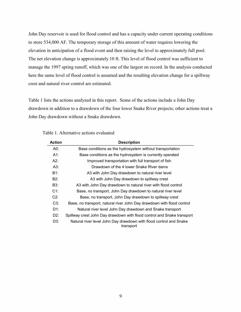
Table 1 lists the actions analyzed in this report. Some of the actions include a John Day
drawdown in addition to a drawdown of the four lower Snake River projects; other actions treat a
John Day drawdown without a Snake drawdown.
Table 1. Alternative actions evaluated
Action DescriptionA0: Base conditions as the hydrosystem without transportationA1: Base conditions as the hydrosystem is currently operatedA2: Improved transportation with full transport of fishA3: Drawdown of the 4 lower Snake River damsB1: A3 with John Day drawdown to natural river levelB2: A3 with John Day drawdown to spillway crestB3: A3 with John Day drawdown to natural river with flood controlC1: Base, no transport, John Day drawdown to natural river levelC2: Base, no transport, John Day drawdown to spillway crestC3: Base, no transport, natural river John Day drawdown with flood controlD1: Natural river level John Day drawdown and Snake transportD2: Spillway crest John Day drawdown with flood control and Snake transportD3: Natural river level John Day drawdown with flood control and Snake
transport

10
3 Measures of fish performance
To assess the performance of the drawdown and full transportation actions relative to the current
hydrosystem operations, three measures of population performance were used. The first two are
probabilities of meeting survival and recovery goals as defined by NMFS Jeopardy Standards.
These were the measures used by PATH. The third measure is the equilibrium level of spawners
for each recovery action. In addition to these measures, the absolute difference between pairwise
comparisons of alternative actions for each measure is reported.
3.1 Survival Standard: 24-year
This measure was developed by PATH and was selected by NMFS as a primary survival standard
for the A-Fish Appendix of the Biological Opinion. It is the fraction of simulation runs for which
the average spawner abundance over a 24 year time period exceeds a predefined threshold for
each index stock. For spring chinook, the survival threshold is 150 or 300 spawners depending
on the river. For fall chinook, two survival thresholds have been proposed 300 and 700 spawners
(Marmorek et al. 1998, Peters et al. 1999).
3.2 Recovery Standard: 48-year
This measure was developed by PATH and was selected by NMFS as a primary recovery
standard. It is the fraction of simulation runs for which the average spawner abundance over the
last 8 years of a 48-year simulation is greater than a specified level, which is 60% of the pre-1971
brood-year average spawner counts in each of the index streams (Marmorek et al. 1998). For fall
chinook two recovery thresholds have been proposed: 2500 and 5100 spawners (Peters et al.
1999).

11
3.3 Equilibrium spawners
The equilibrium measure of the population is the level at which the spawning recruits of a brood
are exactly sufficient to replace their parental brood. With typical salmon life-cycle models, in
the absence of environmental variations and a constant harvest rate, the equilibrium population
level is a stable point that a stock will approach over time. Simply put, the equilibrium is a
measure of the number of fish a habitat can maintain with a specific set of management actions
including hydro operations and fisheries regulations.
3.4 Smolt Passage Measures
The smolt passage measures provide a quantitative description of the direct effects of drawdown
actions on smolt passage. These are valuable because they are not complicated by hypotheses on
the linkage between effects of passage on ocean survival. Passage measures are defined for
migration from the face of lower Granite Dam to the tailrace of Bonneville Dam (used in fall
chinook analysis) or from the top of Lower Granite Pool to the tailrace of Bonneville Dam (used
in the spring chinook analysis). The measures include fish travel time (FTT) in-river survival
(Vn) and the total hydrosystem survival of both transported and in-river passing smolts (Sm). In
addition, reported are the fractions of smolts in Bonneville tailrace that arrived through
transportation (Pb) and in-river passage (1-Pb).
4 Life-cycle Framework
The models used in PATH, by the National Marine Fisheries Service, and the analysis in this
report all are based on a salmon life-cycle model with low number of life history stages.
Generally four important stages are identified (Fig. 1). The first stage is a freshwater spawning
stage that in this report extends from the adult spawners laying eggs in redds to the beginning of
smolt migration. This first freshwater stage characterizes the intrinsic freshwater production of a
stock in terms of the number of progeny (per spawner) that survive through the stage. The second
stage characterizes the migration of the smolts through the hydrosystem from the Lower Granite

12
project to the tailrace of Bonneville Dam. The third stage characterizes the ocean and estuary
survival and ends with the adults at the entrance of the adult bypass channels of Bonneville Dam.
The fourth stage begins with the adults entering the upstream bypass channels and ends just prior
to the spawning event. These four stages describe a complete salmon life cycle. Further divisions
can be made to characterize other sub-stages within each stage, but for the purpose of comparing
the impacts of the drawdown of John Day reservoir to other actions on the hydrosystem, these
four elements are sufficient.
Figure 1. Life cycle of salmon extending from freshwaterproduction stage, P, to hydrosystem survival, Sm, from LowerGranite Dam (LGR) to Bonneville Dam (BON), which includes inriver and transport passage, to ocean survival, So, to upriver adultmigration survival, Sa. S spawners produce R recruits.
The equation related to Figure 1 can be expressed
eq (1) R = S�P�Sm�So�Sa�Ho�Hr
where P is the production of smolts per spawner and may contain some form of density
dependence, Sm is the survival of smolts through the hydrosystem by both in-river and
transportation passage routes, and So is the survival of fish passing through the estuary. Sa is the
survival of the returning adults as they migrate through the hydrosystem, with the inclusion of
prespawning survival and river harvest. Ocean and river harvest mortality are defined as (1- Ho),
and (1- Hr).

13
4.1 Freshwater production (P)
The freshwater production stage describes now many smolts are produced per spawner. The
productivity depends on the number of spawners, with productivity decreasing as the number of
spawners increases. In the PATH analysis, the density effects equation included the possibility of
depensation in which productivity declines at low numbers of spawners. The spawner recruit data
did not reveal any depensation, so functionally PATH used a Ricker density compensation
equation. Here we use the functional form of the Ricker equation to express density effects in
freshwater production:
eq (2) P = exp(afw - b�S)
The afw parameter defines only recruits to the smolt stage so the term is different from the Ricker
“a” coefficient, which defines recruits to the spawning stage. The “b” parameter is the same as in
the Ricker equation and is a measure of the decline in productivity with increasing spawner
numbers.
4.1.1 Density dependence parameter (b)
The density dependent factor b, used in eq(2), is derived from the regression of natural
log(recruits/spawner) versus spawners for spring and fall chinook from the Snake River basin.
Table 2 presents estimates for this parameter and carrying capacity (a/b) for Snake River spring
and fall chinook for the post-1974 period. For spring chinook, the b is taken as the average of the
six Snake River index stocks. For the fall chinook, a single stock is represented, and the
estimates of recruits take harvest into account. For the Snake River fall chinook, the regression
is statistically insignificant (R2 = 0.01). The resulting b is only useful for giving a ball park
estimate of the fish numbers in all of the analyses.

14
Table 2: Ricker coefficients for spring and fall chinook from the Columbia/Snake
River system stocks. Spawners were on redds and recruits were estimated to
mouth of Columbia River. The Snake River spring chinook estimates are the
mean values of 7 index stocks.
Chinook Region Ricker a Ricker b Referencespring Snake River 0.73 0.00174 Schaller et al. 1999spring Upper Columbia 1.04 0.00098 Schaller et al. 1999spring Lower Columbia 1.48 0.00195 Schaller et al. 1999spring Upriver Aggregate 0.41 0.0000016 Schaller et al. 1999
fall Snake River 1.96 0.00027 Peters et al. 1999fall Columbia R. URB 2.65 0.00002 Peters et al. 1999fall Deschutes R. 2.84 0.00037 Peters et al. 1999
4.1.2 Stock equilibrium numbers
To extrapolate from the representative index stocks to the basin-wide impact on the species,
estimates of the number of individual demes or stocks is required. The endangered stocks in the
Snake River Basin are designated as wild and natural stocks. Wild stocks have genetic makeup
unlikely to have been altered by hatchery fish. Natural stocks are naturally spawning fish that
have genetically mixed with hatchery fish. In the Snake River Basin 23 natural and wild spring
chinook and 9 summer chinook stocks were identified by Chapman et al. 1991. Stocks of
hatchery origin include 12 spring chinook stocks and 2 summer chinook stocks. One wild-natural
population of fall chinook has been identified (Chapman et al. 1991). The total number of natural
and wild spring and summer chinook stocks is 32. Members of the Plan for PATH group
suggested a more representative number of stocks is 38. This larger estimate was used in this
report.
15
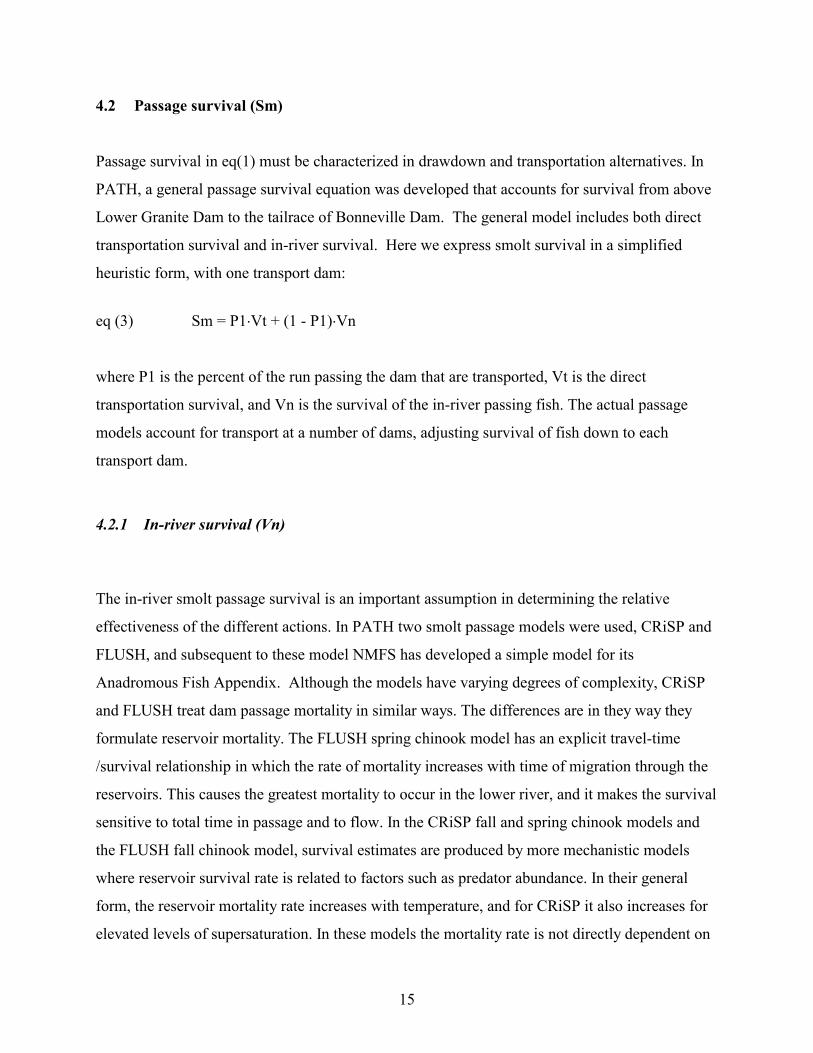
4.2 Passage survival (Sm)
Passage survival in eq(1) must be characterized in drawdown and transportation alternatives. In
PATH, a general passage survival equation was developed that accounts for survival from above
Lower Granite Dam to the tailrace of Bonneville Dam. The general model includes both direct
transportation survival and in-river survival. Here we express smolt survival in a simplified
heuristic form, with one transport dam:
eq (3) Sm = P1�Vt + (1 - P1)�Vn
where P1 is the percent of the run passing the dam that are transported, Vt is the direct
transportation survival, and Vn is the survival of the in-river passing fish. The actual passage
models account for transport at a number of dams, adjusting survival of fish down to each
transport dam.
4.2.1 In-river survival (Vn)
The in-river smolt passage survival is an important assumption in determining the relative
effectiveness of the different actions. In PATH two smolt passage models were used, CRiSP and
FLUSH, and subsequent to these model NMFS has developed a simple model for its
Anadromous Fish Appendix. Although the models have varying degrees of complexity, CRiSP
and FLUSH treat dam passage mortality in similar ways. The differences are in they way they
formulate reservoir mortality. The FLUSH spring chinook model has an explicit travel-time
/survival relationship in which the rate of mortality increases with time of migration through the
reservoirs. This causes the greatest mortality to occur in the lower river, and it makes the survival
sensitive to total time in passage and to flow. In the CRiSP fall and spring chinook models and
the FLUSH fall chinook model, survival estimates are produced by more mechanistic models
where reservoir survival rate is related to factors such as predator abundance. In their general
form, the reservoir mortality rate increases with temperature, and for CRiSP it also increases for
elevated levels of supersaturation. In these models the mortality rate is not directly dependent on
16
the time of passage, although longer fish travel times will result in lower survivals, all other
factors being held constant. The NMFS model assumes no flow/survival relationship, and
reservoir and dam mortality are not distinguished. Reservoir survival is essentially constant for
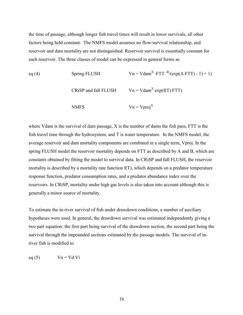
each reservoir. The three classes of model can be expressed in general forms as
eq (4) Spring FLUSH Vn = VdamX �FTT -B/(exp(A�FTT) - 1) + 1)
CRiSP and fall FLUSH Vn = VdamX exp(f(T)�FTT)
NMFS Vn = VprojX
where Vdam is the survival of dam passage, X is the number of dams the fish pass, FTT is the
fish travel time through the hydrosystem, and T is water temperature. In the NMFS model, the
average reservoir and dam mortality components are combined in a single term, Vproj. In the
spring FLUSH model the reservoir mortality depends on FTT as described by A and B, which are
constants obtained by fitting the model to survival data. In CRiSP and fall FLUSH, the reservoir
mortality is described by a mortality rate function f(T), which depends on a predator temperature
response function, predator consumption rates, and a predator abundance index over the
reservoirs. In CRiSP, mortality under high gas levels is also taken into account although this is
generally a minor source of mortality.
To estimate the in-river survival of fish under drawdown conditions, a number of auxiliary
hypotheses were used. In general, the drawdown survival was estimated independently giving a
two part equation: the first part being survival of the drawdown section, the second part being the
survival through the impounded sections estimated by the passage models. The survival of in-
river fish is modified to
eq (5) Vn = Vd�Vi

17
where Vd is the survival through a drawdown section of the river under a specific drawdown
alternative, and Vi is the survival through the impounded sections.
4.2.2 Natural River Drawdown survival (Vd )
A great deal of uncertainty exists over what survivals will be in free-flowing river segments after
reservoirs are drawn-down to natural river levels. In PATH, upper and lower bound survivals
were used for the drawn-down Snake reservoirs in an effort to characterize the range of
uncertainty. These estimates were developed by applying direct or indirect estimates of survival
through existing free-flowing reaches to future drawn-down reaches on a per km basis. For fall
chinook PIT tag survivals from 1995-1998 were used. These survival estimates encompass both
free-flowing and impounded segments, and two methods were used to extract survivals through
the free-flowing segment. (Peters et al. 1999). For spring chinook, free-flowing survival
estimates were based on survival estimates from the Whitebird trap in the Salmon River to the
uppermost dam, either Ice Harbor (1966-1969) or Lower Granite (1993-1996) (Marmorek and
Peters 1998). For spring chinook, the John Day estimates were derived by taking survival per km
from the Snake River studies and adjusting to the length of the John Day reservoir. For fall
chinook, the John Day estimates were derived from the passage models under drawdown
conditions. Upper and Lower bound survival estimates are provided in Table 3.
Table 3. Drawdown survivals Vd through free-flowing reaches of the SnakeRiver and John Day reservoir.
Chinook type river segment Lower estimate Upper estimatespring Snake R. 0.85 0.96
fall Snake R. 0.61 0.90spring John Day 0.90 0.98
fall John Day 0.87 0.87
Total system survival Sm generated from CRiSP for the different alternatives are given in Tables
21 and 22.

18
4.2.3 Spill Crest and Food Control Drawdown survival (Vd)
To estimate survival in John Day pool under a spillway crest drawdown and under natural river
with flood control, the CRiSP passage model (Anderson et al. 1996) was used. In this model
system reservoir elevation and river flow are used to estimate water velocity. The water velocity
in turn is used to predict fish velocity, and this in turn is used to predict fish reservoir survival.
Estimating the impacts of spillway crest drawdown and natural river drawdown under flood
control then results in estimating the impact on fish velocity which effects survival. These
capabilities are integral to the CRiSP model and so estimating these special conditions involved
only defining reservoir elevations. Estimating the change in reservoir elevation with flood
control involved additional calculations, which are detailed below.
The CRiSP model represents reservoirs through a number of rectangles giving the reservoir side
and thalweg slopes as illustrated in Figure 2. The tailwater and forebay ends of the reservoir are
set at the actual elevations giving an average thalweg gradient. In addition the angle of sides are
set to approximate the slopes of the reservoir banks. As the reservoir is drawn down the upstream
portion enters a free-flowing stage where the velocity is constant determined by drag properties
of the streambed. In these calculations the free-flowing velocity, Ufree, was set at 5 ft/s.
Figure 2. Reservoir with free-flowing and impounded portions. Theterms are reservoir elevation E, length L, volume V(E), flow F, andstream velocity Ufree.

19
Under these model conditions, the reservoir water velocity increases in an approximately linear
manner with elevation drawdown. At natural river drawdown levels, though, the river velocity
reaches a maximum as velocity is determined by the drag of the channel (Table 4).
Table 4: Water velocities (miles/day) for different flows and pool elevations
Action Elevationdrop (ft)
Normal flow (236kcfs)
High flow (400kcfs)
Full pool 0 16 25Spillway crest 50 53 80Natural River 100 90 95
To determine the effects of flood control on river elevation and velocity the relationship between
elevation and velocity is used. The average river velocity, U, at elevation z is equal to the flow, F,
divided by the cross-sectional area, A:
eq (6) U(z) = F/A.
The velocity under flood control, in which the elevation is raised to absorb the flood control
water, can be expressed as
eq (7) U(z1) = L�F/(V + L�F/U(z0)).
Where z0 and z1 are the base and flood control elevations, L = 76.4 miles is the John Day
reservoir length, F = 500 kcfs is the flow at which flood control is typically required and V =
534,000 acre-feet is the flood control volume. If the high flow at a natural river elevation gives a
velocity of 100 miles/day or approximately 6 ft/s then the velocity after absorbing the flood
control volume becomes about 50 miles/day or 3 ft/sec. Since velocity is approximately linearly
related to elevation, the change in reservoir elevation (from natural river conditions) with flood
control can be estimated. The elevation under natural river would rise to about the spill crest
elevation, and under a spill crest drawdown flood control would raise the elevation another 10 to
15 feet above the spillway crest. These estimates are approximate since they are developed on the
assumption of simplified reservoir geometry, and the natural river segment velocity is fixed. The
20
hydraulics is sufficient to estimate the impacts of natural river level flood control on smolt
passage.
4.3 Ocean/estuary survival (So)
The survival of fish, between the time they leave the tailrace of Bonneville dam as smolts and
return to the fish ladders of Bonneville dam as spawning adults, is an important life stage that
exhibits a large range of variability from year to year. A number of assumptions in PATH were
developed to characterize the possible factors that determine survival during the ocean residence
life stage. Of particular importance, are the effects of hydrosystem passage route on ocean
survival. Because fish pass through the hydrosystem in transportation and as run of the river fish,
there is the possibility that the ocean survival is different for fish from each passage route. The
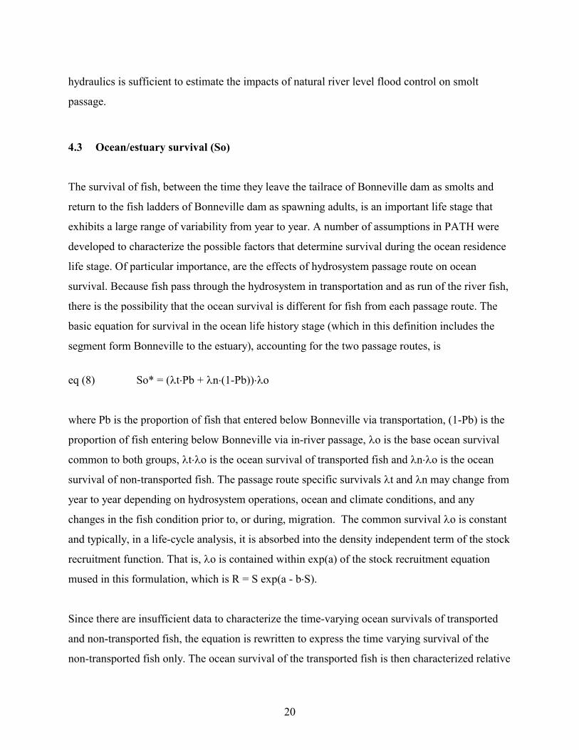
basic equation for survival in the ocean life history stage (which in this definition includes the
segment form Bonneville to the estuary), accounting for the two passage routes, is
eq (8) So* = (�t�Pb + �n�(1-Pb))��o
where Pb is the proportion of fish that entered below Bonneville via transportation, (1-Pb) is the
proportion of fish entering below Bonneville via in-river passage, �o is the base ocean survival
common to both groups, �t��o is the ocean survival of transported fish and �n��o is the ocean
survival of non-transported fish. The passage route specific survivals �t and �n may change from
year to year depending on hydrosystem operations, ocean and climate conditions, and any
changes in the fish condition prior to, or during, migration. The common survival �o is constant
and typically, in a life-cycle analysis, it is absorbed into the density independent term of the stock
recruitment function. That is, �o is contained within exp(a) of the stock recruitment equation
mused in this formulation, which is R = S exp(a - b�S).
Since there are insufficient data to characterize the time-varying ocean survivals of transported
and non-transported fish, the equation is rewritten to express the time varying survival of the
non-transported fish only. The ocean survival of the transported fish is then characterized relative
21
to the non-transported fish survival. Also the base term �o can be ignored in the deterministic
model because in the pairwise comparisons of actions, ratios of productivity are taken and so �o
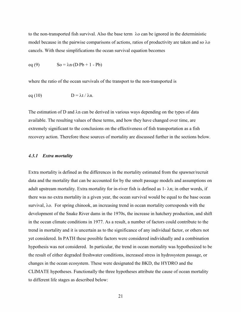
cancels. With these simplifications the ocean survival equation becomes
eq (9) So = �n�(D�Pb + 1 - Pb)
where the ratio of the ocean survivals of the transport to the non-transported is
eq (10) D = �t / �n.
The estimation of D and �n can be derived in various ways depending on the types of data
available. The resulting values of these terms, and how they have changed over time, are
extremely significant to the conclusions on the effectiveness of fish transportation as a fish
recovery action. Therefore these sources of mortality are discussed further in the sections below.
4.3.1 Extra mortality
Extra mortality is defined as the differences in the mortality estimated from the spawner/recruit
data and the mortality that can be accounted for by the smolt passage models and assumptions on
adult upstream mortality. Extra mortality for in-river fish is defined as 1- �n; in other words, if
there was no extra mortality in a given year, the ocean survival would be equal to the base ocean
survival, �o. For spring chinook, an increasing trend in ocean mortality corresponds with the
development of the Snake River dams in the 1970s, the increase in hatchery production, and shift
in the ocean climate conditions in 1977. As a result, a number of factors could contribute to the
trend in mortality and it is uncertain as to the significance of any individual factor, or others not
yet considered. In PATH these possible factors were considered individually and a combination
hypothesis was not considered. In particular, the trend in ocean mortality was hypothesized to be
the result of either degraded freshwater conditions, increased stress in hydrosystem passage, or
changes in the ocean ecosystem. These were designated the BKD, the HYDRO and the
CLIMATE hypotheses. Functionally the three hypotheses attribute the cause of ocean mortality
to different life stages as described below:

22
BKD hypothesis states that the extra mortality is associated with a change in the wild fish
condition, possibly from disease such as bacterial kidney disease (BKD) resulting from
increased hatchery production beginning in the late 1970s. Under this hypothesis the extra
mortality is endemic to the wild Snake River chinook and is here to stay under changes in
the hydrosystem operations.
HYDRO hypothesis postulates that the extra mortality is associated with the hydrosystem
and specifically the Snake River portion of the hydrosystem. Under this hypothesis it
could be associated with the cumulative stress in hydrosystem passage. Consequentially,
in this hypothesis removing dams removes the stress and results in higher survival below
the hydrosystem.
CLIMATE hypothesis postulates that the extra mortality is associated with a
climate/ocean regime shift that occurred in the late 1970s. Under this hypothesis the extra
mortality only disappears if the climate shifts back to a fish-favorable ocean regime and
the effect is independent of any changes made to the hydrosystem.
Some details of the linkages between life-stage survivals were developed in PATH, but are not
important to explore here. What is important though, is that specific mechanisms have not been
identified for any of the hypotheses, nor has significant correlation between of variables related
to the hypotheses and ocean survival of non-transported fish been demonstrated. As a result of
this inability to clarify the mechanisms, the results from PATH should be considered as
exploratory of the range of possible consequences.
The range of ocean survivals, expressed as the extra mortality factor as 1- �n, was derived in
PATH from the combination of a life-cycle model with a passage model for the spring and fall
chinook. The essential survivals are given in Table 5. Note the examples in the table characterize
ocean survival as affected by the extra mortality factor. The possible levels of extra mortality
depend on mortality assumptions in the retrospective analysis of stock dynamics. These details

23
are beyond the scope of the deterministic analysis here. Table 5 is intended to illustrate the
general ranges over which extra mortality contributes to ocean survival of fish.
Table 5: Characteristic ocean survival factor �n, as determined by extra mortality,under different passage model hypotheses using the Delta model developed inPATH (Hinrichsen and Paulsen 1998) with ranges (min-max). Spring �nestimates from regressions of Vn vs. �n with Vn = 0.2 for 1975-1990 and Vn =0.4 for 1952-1990 period. Fall chinook estimates from spawner/recruit analysis(Peters et al. 1999).
Chinook years CRiSP FLUSHspring 1952-1990 0.7 (0.1-1.5) 0.75 (0.1-1.5)spring 1975-1990 0.4 (0.1-1.8) 0.75 (0.2-1.31)
fall 1964-1991 1 1
4.3.2 Delayed mortality
The transportation efficiency factor D, which is the ratio of ocean survival of transported fish to
the ocean survival of non-transported fish, is critical in determining the relative effectiveness of
recovery actions. In PATH, this factor has been referred to as the delayed mortality because
mortality is thought to occur somewhere below Bonneville Dam as a result of smolts being
transported. If D equals one, then the survival from in-river and transport hydrosystem passage
routes are equal and fish experience no delayed mortality as a result of being transported. If D is
less than one, then the transported fish suffer a delayed mortality relative to the in-river fish.
Exactly where this mortality occurs is unknown though, and the mechanisms resulting in higher
mortality of transported fish are unknown. Observed survivals of fish held after transportation
range between about 80% and 100% (Reference). Furthermore, radio tracking studies of
transported and in-river fish tagged at Bonneville Dam indicate equal survivals in the two groups
down to the estuary where the salt water makes the radio tag inoperative.
Estimating D has been problematic for both spring and fall chinook. For spring chinook, D is
calculated from estimates of the in-river smolt survival times the ratio of returning adults marked
as smolts for transportation and in-river passage groups. As a result, estimates of D have several
24
critical assumptions that increase the uncertainty, especially in the early years of the
transportation program, prior to the development of the PIT tag technology. In the early years of
the transportation program, a large fraction of the transport studies control fish were transported
at a lower dam so the transport to control ratio of the returning adults was actually a comparison
of returns of fish from two transport sites. The use of these data is problematic for assessing the
difference of transport and in-river fish because further assumptions are required to correct for
the transported control fish. Furthermore, recent transport studies indicate that the timing of
arrival of fish to the estuary has a significant impact on their ocean survival (Hinrichsen et al.
1996). PATH did not fully address or resolve these issues and so the estimates of D are highly
uncertain. Two basic approaches were taken to estimate D in PATH, and it was determined the
most important factor was the choice of smolt passage model, FLUSH or CRiSP. Additionally, in
the NMFS A-fish Appendix a high value of D was explored, based on the recent PIT tag studies.
Although these details are important in evaluating the historical D, the most important
hypotheses concern the D current and future levels. The possible ways that D could have changed
from the early years of fish transportation is summarized in the hypotheses listed in Table 6. For
spring chinook, the dividing year between the early and the current levels of D is taken as 1980.
Prior to 1980 the transportation system was experimental and significant handling problems that
stressed the fish were evident at the transport dams (reference). The geometric averages of D for
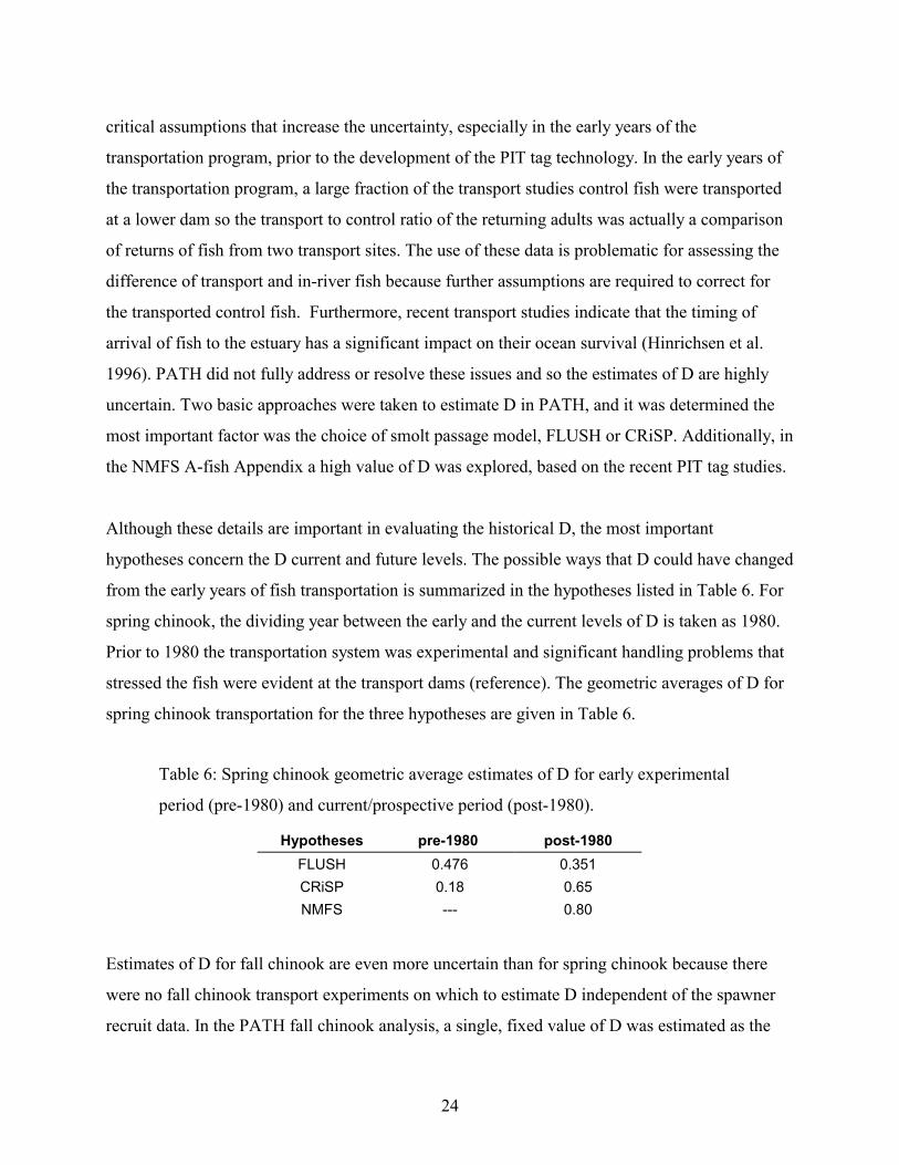
spring chinook transportation for the three hypotheses are given in Table 6.
Table 6: Spring chinook geometric average estimates of D for early experimental
period (pre-1980) and current/prospective period (post-1980).
Hypotheses pre-1980 post-1980FLUSH 0.476 0.351CRiSP 0.18 0.65NMFS --- 0.80
Estimates of D for fall chinook are even more uncertain than for spring chinook because there
were no fall chinook transport experiments on which to estimate D independent of the spawner
recruit data. In the PATH fall chinook analysis, a single, fixed value of D was estimated as the
25
fitting parameter in the life-cycle analysis based on the spawner/recruit data and the modeled in-
river passage. The estimated value of D ranged from 0.03 to 0.52. In addition, a D value for fall
chinook transported from McNary Dam was estimated from both a life-cycle analysis and
transport-to-control studies at this dam. These values were considerably higher than the estimates
for Snake River fall chinook obtained from the life-cycle model. McNary Dam D values ranged
between 0.6 and 6, with a geometric mean of 1.7. In PATH, five sets were considered for the
change D from the retrospective to the prospective periods (Table 7). In effect, these hypotheses
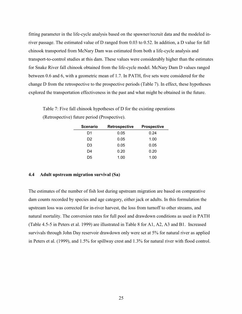
explored the transportation effectiveness in the past and what might be obtained in the future.
Table 7: Five fall chinook hypotheses of D for the existing operations
(Retrospective) future period (Prospective).
Scenario Retrospective ProspectiveD1 0.05 0.24D2 0.05 1.00D3 0.05 0.05D4 0.20 0.20D5 1.00 1.00
4.4 Adult upstream migration survival (Sa)
The estimates of the number of fish lost during upstream migration are based on comparative
dam counts recorded by species and age category, either jack or adults. In this formulation the
upstream loss was corrected for in-river harvest, the loss from turnoff to other streams, and
natural mortality. The conversion rates for full pool and drawdown conditions as used in PATH
(Table 4.5-5 in Peters et al. 1999) are illustrated in Table 8 for A1, A2, A3 and B1. Increased
survivals through John Day reservoir drawdown only were set at 5% for natural river as applied
in Peters et al. (1999), and 1.5% for spillway crest and 1.3% for natural river with flood control.

26
Table 8: Conversion rate of adult migration survival (Sa) from Bonneville Dam
tailrace to the spawning grounds (Marmorek et al. 1996, Peters et al. 1999).
A1 A2 A3 B1 B2 B3 C1 C2 C3Spring 0.67 0.67 0.77 0.81 0.79 0.80 0.70 0.69 0.69
Fall 0.42 0.42 0.83 0.87 0.87 NA 0.44 0.43 NA
5 Bayesian life-cycle analysis
To model the survival and recovery probabilities, a detailed life-cycle model adapted from the
PATH analysis has been used. The methods of the PATH analysis are described in Marmorek,
Peters and Parnell (eds.) (1998) and Peters Marmorek and Parnell (eds) (1999). The model uses
the basic life-cycle dynamics expressed by eq (1) with a Ricker density dependence similar to eq
(13). The PATH analysis was set up to explore the consequences of different assumptions on life
stages, and in PATH two basic passage models were explored along with different assumptions
on how life stages were connected and represented.
A retrospective analysis of spring and fall chinook was conducted in PATH using the historical
spawner recruit and passage data to characterize detailed hypotheses on the life stages. In
addition, in PATH a prospective analysis was developed to project the time evolution of stocks
under differing assumptions about the effects of actions. Using a Bayesian analysis, the different
hypotheses could be weighted with output of the probabilities of meeting survival and recovery
goals.
Selected results from the PATH analysis are used in this report. Specifically, the retrospective
analysis is used to characterize the life stage parameters for the deterministic analysis presented
in this report. In addition, the prospective analysis has been applied to produce survival and
recovery probabilities and equilibrium spawner levels under different weightings of the
hypotheses.

27
The results of the life-cycle analyses depend on hypotheses used and the weightings applied to
each hypothesis. In PATH a large number of hypotheses on life stage parameter values and
functional forms of the linkages of ocean survival to the passage survival and the freshwater
production life stage were evaluated. In this analysis a reduced set of the most influential
hypotheses are included in evaluating survival and recovery probabilities and equilibrium
population levels.
5.1 Actions evaluated for spring and fall chinook
The PATH Bayesian Simulation Model (BSM) was only used to evaluate action A1, A2, A3, and
B1. In addition, for assessing probabilities of recovery over time, Actions A3 and B1 were
evaluated under different delays of implementing the actions (Table 9).
Table 9: Actions evaluated with the PATH Bayesian model
Action DescriptionA1: Uses the existing transportation rulesA2: Maximizes transportation using current system configuration
A3(3yr): Drawdown of four Snake River dams (3-year delay)A3(8yr): Drawdown of four Snake River dams (8-year delay)B1(10yr): Drawdown of four Snake River dams (3-year delay) and drawdown of
John Day Dam (10-year delay)B1(15yr): Drawdown of four Snake River dams (8-year delay) and drawdown of
John Day Dam (15-year delay)
5.2 Hypotheses
The most important hypotheses concerned the survival of smolts through the hydrosystem and
the survival of smolts after departing the hydrosystem. Because some smolts migrate through the
river while others are collected at dams and transported, survival through both hydrosystem
passage routes, and the associated survivals below the hydrosystem, must be considered.
Scenarios to evaluate different factors controlling these hypotheses are listed in Table 10 for
spring chinook and Table 11 for fall chinook.

28
5.2.1 Spring chinook hypotheses
The smolt passage models applied in the Bayesian life-cycle model are detailed in Section 4.2.
Each passage model is grouped with an assumption on D that characterizes delayed mortality in
transportation. CRiSP is paired with midrange D values and FLUSH is paired with low D values.
In addition, model runs were conducted with the assumption that D was high. The values for D
are described in Section 4.3.2. Three hypotheses on the source of the extra mortality were
considered in the Bayesian analysis, the BKD, CLIMATE and HYDRO hypotheses. These are
described in Section 4.3.1.
Two life-cycle models were considered in this analysis: the Alpha and Delta models, which
differed primarily in the characterization of climatic/ocean change. The Delta model assumed
that decadal scale climate/ocean changes in Snake River spring have the same pattern as
observed in the mid- and lower Columbia spring chinook. The Alpha model characterized ocean
variation through decadal climate indices, the PAPA drift index, and river flow at Astoria.
A lower level hypothesis in the modeling system involves the estimated time required to
implement drawdown actions. This affects the success of the drawdown as a recovery action. In
the analysis two periods were considered: 3 and 8 year delays for drawing down the four Snake
River dams and 10 and 15 year delays for drawing down the four Snake River reservoirs plus the
John Day reservoir. Assumptions were also included to characterize the amount of time before
the drawdown reservoirs reach equilibrium in terms of the riverine habitat. Two periods were
assumed: 2 and 10 years.
29
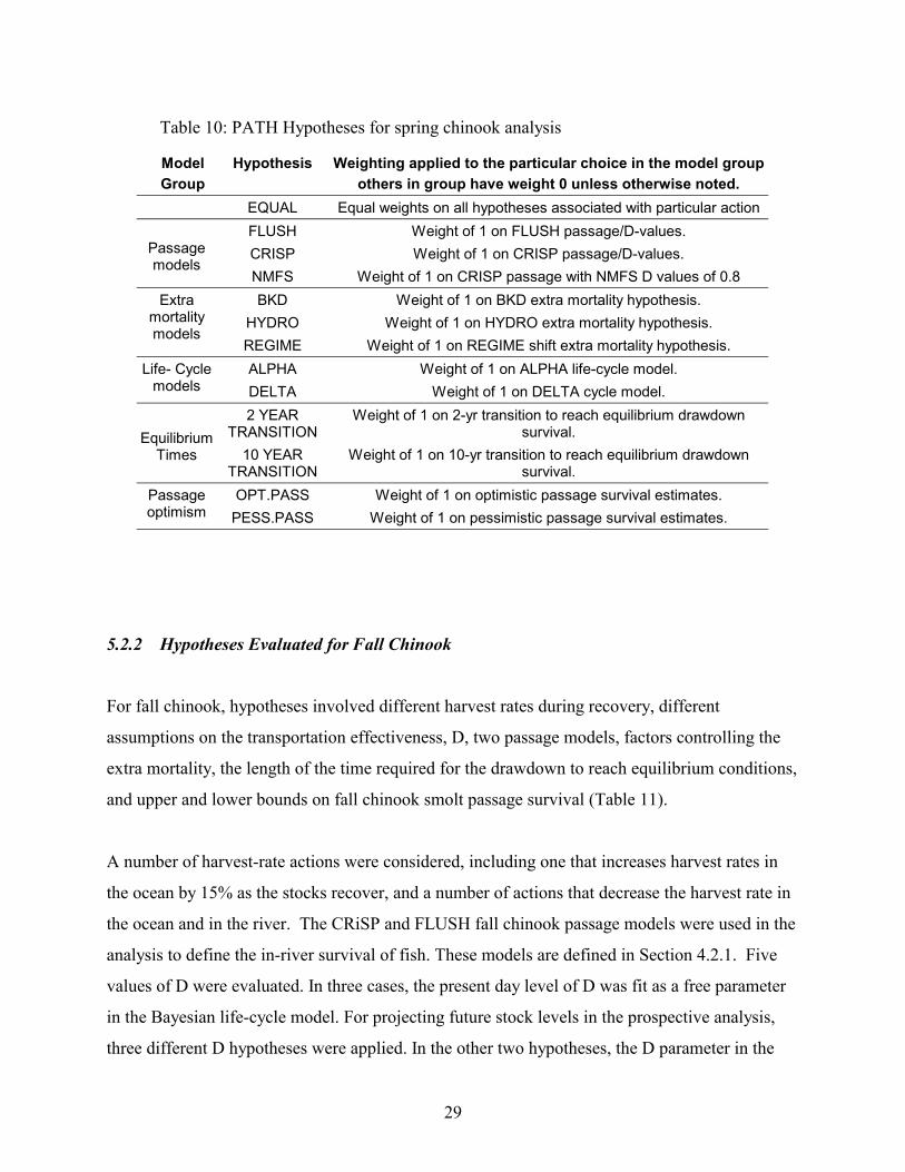
Table 10: PATH Hypotheses for spring chinook analysis
ModelGroup
Hypothesis Weighting applied to the particular choice in the model groupothers in group have weight 0 unless otherwise noted.
EQUAL Equal weights on all hypotheses associated with particular actionFLUSH Weight of 1 on FLUSH passage/D-values.CRISP Weight of 1 on CRISP passage/D-values.Passage
modelsNMFS Weight of 1 on CRISP passage with NMFS D values of 0.8BKD Weight of 1 on BKD extra mortality hypothesis.
HYDRO Weight of 1 on HYDRO extra mortality hypothesis.Extra
mortalitymodels
REGIME Weight of 1 on REGIME shift extra mortality hypothesis.ALPHA Weight of 1 on ALPHA life-cycle model.Life- Cycle
models DELTA Weight of 1 on DELTA cycle model.2 YEAR
TRANSITIONWeight of 1 on 2-yr transition to reach equilibrium drawdown
survival.EquilibriumTimes 10 YEAR
TRANSITIONWeight of 1 on 10-yr transition to reach equilibrium drawdown
survival.OPT.PASS Weight of 1 on optimistic passage survival estimates.Passage
optimism PESS.PASS Weight of 1 on pessimistic passage survival estimates.
5.2.2 Hypotheses Evaluated for Fall Chinook
For fall chinook, hypotheses involved different harvest rates during recovery, different
assumptions on the transportation effectiveness, D, two passage models, factors controlling the
extra mortality, the length of the time required for the drawdown to reach equilibrium conditions,
and upper and lower bounds on fall chinook smolt passage survival (Table 11).
A number of harvest-rate actions were considered, including one that increases harvest rates in
the ocean by 15% as the stocks recover, and a number of actions that decrease the harvest rate in
the ocean and in the river. The CRiSP and FLUSH fall chinook passage models were used in the
analysis to define the in-river survival of fish. These models are defined in Section 4.2.1. Five
values of D were evaluated. In three cases, the present day level of D was fit as a free parameter
in the Bayesian life-cycle model. For projecting future stock levels in the prospective analysis,
three different D hypotheses were applied. In the other two hypotheses, the D parameter in the

30
retrospective and prospective analyses were specified. The three extra mortality hypotheses were
evaluated as in the spring chinook. It should be noted though that under low values of D, as are
derived from the MLE estimation of D, the extra mortality is essentially zero. Only when D is
large (~ 1) is an extra mortality factor required to account for the decline in the fall chinook. Two
transition periods were evaluated for the time for each drawn-down reservoir to reach a
functioning state that stabilizes survival. Finally, the models were run with combinations of
juvenile passage survival representing low and high levels of survival.
Table 11: Hypotheses used in the fall chinook analysis
Hypothesis WeightsEQUAL All hypotheses weighted equallyBase(-/-) Base ocean and in-river harvest+15%/- (% increase in ocean harvest/% increase in in-river harvest)-15%/- (% increase in ocean harvest/% increase in in-river harvest)-50%/- (% increase in ocean harvest/% increase in in-river harvest)-75%/- (% increase in ocean harvest/% increase in in-river harvest)
-50%/-50% (% increase in ocean harvest/% increase in in-river harvest)-75%/-50% (% increase in ocean harvest/% increase in in-river harvest)
CRISP CRISP passage modelFLUSH FLUSH passage model
D1 Retro D value is MLE, prospective D=0.24D2 Retro D values is MLE, prospective D=1.0D3 Retro D value is MLE, prospective from posterior distributionD4 Retro D=.2, prospective D=.2D5 Retro D=1.0, prospective D=1.0
REGIME Regime shift extra mortality hypothesisBKD BKD extra mortality hypothesis
HYDRO HYDRO extra mortality hypothesis2YR.TRANSITION 2-year transition to equilibrium juvenile survival under drawdown10YR.TRANSITION 10-year transition to equilibrium juvenile survival under drawdown
LOW.EJUV juvenile survival lower bound in Snake and John Day drawdownHIGH.EJUV juvenile survival upper bound in Snake and John Day drawdown

31
5.2.3 Weighting hypotheses
The Bayesian life-cycle model combined competing, and sometimes mutually exclusive,
hypotheses giving probabilities of meeting recovery goals and levels of escapement under
equilibrium conditions. To investigate the influence of particular hypotheses on a life stage
component of survival, or for a set of hypotheses for several life stages, any of the hypotheses in
the life-cycle model can be given different weights. For example, by giving the FLUSH model a
weight of one and the CRiSP model a weight of zero the patterns of the stocks over a 48 year
future is modeled under the FLUSH passage model hypothesis only. The neutral case gives equal
weighting to each competing hypothesis. Decision analysis generally is not designed to give a
single answer on the response of a stock to an action, such as drawdown. By combining all the
hypotheses with, or without, equal weighting, it is designed to identify which actions are the most
robust to the uncertainties in the models.
In the decision analysis approach, differing hypotheses were combined to evaluate actions. The
numbers of hypotheses for the spring chinook BSM analysis are given in Table 12.
Table 12: Number of hypotheses under each action
Action Total Hypotheses
A1 36A2 36A3 144B1 144

32
5.3 BSM Results
5.3.1 Probability of Survival and Recovery
Probabilities of survival and recovery for spring and fall chinook under each of the major
alternatives and under different weightings of the important hypotheses are detailed in Table 13
through Table 16. The results are based on the Bayesian life-cycle model. Also provided in Table
17 and 18 are the relative risk expressed as the change in probability in taking Action A3 instead
of B1 and loss of probability in taking A1 instead of A3. Table 19 gives the equilibrium stock
levels for the six Snake River index stocks under the different actions and under different
weightings of the hypotheses.
Table 13: Spring chinook 24-year survival probability mean values.
Hypothesis weighting A1 A2 A3(3yr) A3(8yr) B1(10yr) B1(15yr)EQUAL 0.673 0.668 0.725 0.698 0.723 0.702FLUSH 0.582 0.563 0.689 0.632 0.685 0.640CRISP 0.730 0.732 0.760 0.741 0.755 0.746NMFS 0.707 0.709 0.725 0.720 0.728 0.721BKD 0.607 0.606 0.674 0.642 0.670 0.644HYD 0.758 0.746 0.794 0.773 0.794 0.780
REGIME 0.654 0.653 0.705 0.677 0.704 0.683ALPHA 0.647 0.647 0.712 0.682 0.706 0.684DELTA 0.699 0.690 0.737 0.713 0.740 0.720
2YR.TRANSITION 0.673 0.668 0.739 0.708 0.739 0.71110YR.TRANSITION 0.673 0.668 0.710 0.687 0.706 0.694
OPT.PASS 0.693 0.693 0.751 0.727 0.749 0.728PESS.PASS 0.654 0.644 0.698 0.668 0.697 0.677

33
Table 14: Spring chinook 48-year recovery probability mean values.
Hypothesis weighting A1 A2 A3(3yr) A3(8yr) B1(10yr) B1(15yr)EQUAL 0.533 0.514 0.787 0.795 0.822 0.811FLUSH 0.368 0.328 0.863 0.880 0.911 0.897CRISP 0.615 0.614 0.789 0.786 0.807 0.815NMFS 0.616 0.599 0.708 0.719 0.749 0.721BKD 0.375 0.364 0.668 0.677 0.709 0.699HYD 0.624 0.594 0.858 0.864 0.895 0.884
REGIME 0.600 0.582 0.834 0.845 0.863 0.850ALPHA 0.468 0.451 0.728 0.747 0.779 0.760DELTA 0.598 0.577 0.846 0.843 0.865 0.863
2YR.TRANSITION 0.533 0.514 0.790 0.793 0.822 0.81210YR.TRANSITION 0.533 0.514 0.784 0.798 0.822 0.811
OPT.PASS 0.568 0.552 0.834 0.844 0.862 0.861PESS.PASS 0.498 0.475 0.739 0.747 0.783 0.762
Table 15: Fall chinook probability of meeting a 24-year survival standard.
Hypothesis weighting A2 A3(3yr) A3(8yr) B1(10yr) B1(15yr)EQUAL 0.940 0.955 0.946 0.952 0.949Base(-/-) 0.924 0.948 0.935 0.944 0.939+15%/- 0.918 0.947 0.932 0.942 0.937-15%/- 0.929 0.950 0.938 0.946 0.942-50%/- 0.941 0.954 0.946 0.951 0.948-75%/- 0.946 0.955 0.949 0.952 0.950
-50%/-50% 0.961 0.966 0.963 0.965 0.964-75%/-50% 0.964 0.967 0.965 0.966 0.965
CRISP 0.915 0.944 0.930 0.940 0.935FLUSH 0.964 0.966 0.963 0.965 0.964
D1 0.993 0.991 0.993 0.991 0.992D2 0.999 0.997 0.997 0.998 0.998D3 0.830 0.918 0.885 0.907 0.895D4 0.922 0.942 0.929 0.938 0.933D5 0.956 0.955 0.952 0.953 0.952
REGIME 0.945 0.961 0.952 0.958 0.955BKD 0.938 0.958 0.949 0.955 0.952
HYDRO 0.938 0.963 0.952 0.959 0.9552YR.TRANSITION 0.940 0.956 0.948 0.953 0.950
10YR.TRANSITION 0.940 0.954 0.945 0.951 0.949LOW.EJUV 0.940 0.952 0.943 0.948 0.945HIGH.EJUV 0.940 0.958 0.950 0.956 0.953

34
Table 16: Fall chinook probability of meeting the 48-yr recover standard.
Hypothesis weighting A2 A3(3yr) A3(8yr) B1(10yr) B1(15yr)EQUAL 0.643 0.955 0.954 0.969 0.969Base(-/-) 0.578 0.945 0.944 0.961 0.961+15%/- 0.555 0.94 0.939 0.958 0.958-15%/- 0.601 0.949 0.948 0.964 0.964-50%/- 0.672 0.96 0.959 0.973 0.973-75%/- 0.698 0.964 0.963 0.976 0.976
-50%/-50% 0.723 0.969 0.968 0.979 0.979-75%/-50% 0.749 0.972 0.971 0.982 0.982
CRiSP 0.557 0.956 0.956 0.967 0.967FLUSH 0.729 0.954 0.952 0.971 0.971
D1 0.917 1 1 1 1D2 1 1 1 1 1D3 0.351 1 1 1 1D4 0.437 0.999 0.999 0.999 0.999D5 0.737 0.867 0.864 0.908 0.909
REG 0.735 0.984 0.984 0.991 0.991BKD 0.665 0.936 0.934 0.954 0.954HYD 0.665 1 1 1 1
2YR.TRANS 0.643 0.955 0.956 0.97 0.9710YR.TRANS 0.643 0.955 0.953 0.969 0.969LOW.EJUV 0.643 0.938 0.937 0.955 0.955HIGH.EJUV 0.643 0.973 0.972 0.984 0.984
5.3.2 Relative risks

35
Relative risks are the difference in probabilities of survival and recovery between two action for
a given set of weightings of the hypotheses. A positive value indicates the probability of meeting
a measure increases by the amount. Relative risk for a Snake River drawdown compared to a
Snake River drawdown with a John Day drawdown to natural river level is defined by the
difference in the probabilities for A3 and A1, i.e. B1 - A3. The relative risk of Snake River
drawdown compared to transportation is defined by the difference in probabilities for A3 and A1,
i.e. A3 - A1. Table (17) gives relative risk for spring chinook and Table (18) gives relative risk
for fall chinook.
Table 17: Relative risk for spring chinook. B1-A3 is gain in probability of
meeting standard due to taking action B1 over action A3. A3-A1 is gain in
probability of meeting standard due to taking action A3 over action A1.
24-Year Survival 48-Year Recovery
Hypothesis weighting B1- A3 A3- A1 B1- A3 A3- A1EQUAL 0.0010 0.0385 0.0255 0.2580FLUSH 0.0020 0.0785 0.0325 0.5035CRISP 0 0.0205 0.0235 0.1725NMFS 0.0020 0.0155 0.0215 0.0975BKD -0.0010 0.0510 0.0315 0.2975HYD 0.0035 0.0255 0.0285 0.2370
REGIME 0.0025 0.0370 0.0170 0.2395ALPHA -0.0020 0.0500 0.0320 0.2695DELTA 0.0050 0.0260 0.0195 0.2465
2YR.TRANSITION 0.0015 0.0505 0.0255 0.258510YR.TRANSITION 0.0015 0.0255 0.0255 0.2580
OPT.PASS -0.0005 0.0460 0.0225 0.2710PESS.PASS 0.0040 0.0290 0.0295 0.2450
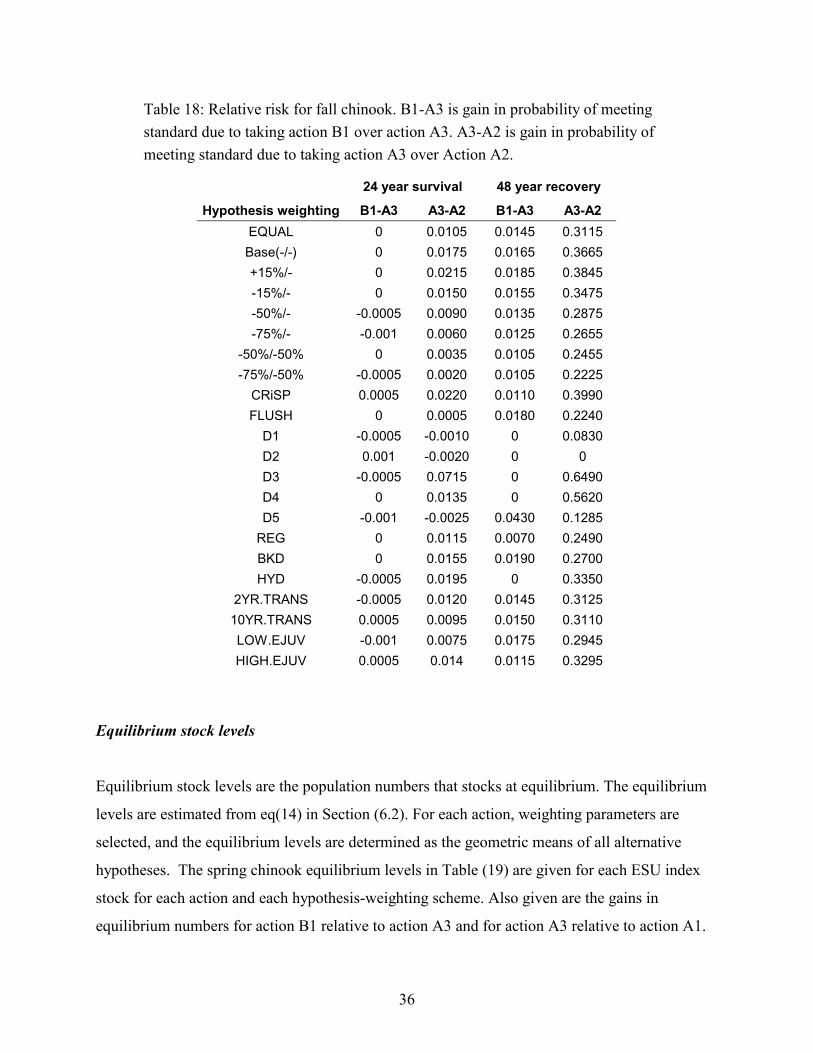
36
Table 18: Relative risk for fall chinook. B1-A3 is gain in probability of meetingstandard due to taking action B1 over action A3. A3-A2 is gain in probability ofmeeting standard due to taking action A3 over Action A2.
24 year survival 48 year recovery
Hypothesis weighting B1-A3 A3-A2 B1-A3 A3-A2EQUAL 0 0.0105 0.0145 0.3115Base(-/-) 0 0.0175 0.0165 0.3665+15%/- 0 0.0215 0.0185 0.3845-15%/- 0 0.0150 0.0155 0.3475-50%/- -0.0005 0.0090 0.0135 0.2875-75%/- -0.001 0.0060 0.0125 0.2655
-50%/-50% 0 0.0035 0.0105 0.2455-75%/-50% -0.0005 0.0020 0.0105 0.2225
CRiSP 0.0005 0.0220 0.0110 0.3990FLUSH 0 0.0005 0.0180 0.2240
D1 -0.0005 -0.0010 0 0.0830D2 0.001 -0.0020 0 0D3 -0.0005 0.0715 0 0.6490D4 0 0.0135 0 0.5620D5 -0.001 -0.0025 0.0430 0.1285
REG 0 0.0115 0.0070 0.2490BKD 0 0.0155 0.0190 0.2700HYD -0.0005 0.0195 0 0.3350
2YR.TRANS -0.0005 0.0120 0.0145 0.312510YR.TRANS 0.0005 0.0095 0.0150 0.3110LOW.EJUV -0.001 0.0075 0.0175 0.2945HIGH.EJUV 0.0005 0.014 0.0115 0.3295
Equilibrium stock levels
Equilibrium stock levels are the population numbers that stocks at equilibrium. The equilibrium
levels are estimated from eq(14) in Section (6.2). For each action, weighting parameters are
selected, and the equilibrium levels are determined as the geometric means of all alternative
hypotheses. The spring chinook equilibrium levels in Table (19) are given for each ESU index
stock for each action and each hypothesis-weighting scheme. Also given are the gains in
equilibrium numbers for action B1 relative to action A3 and for action A3 relative to action A1.
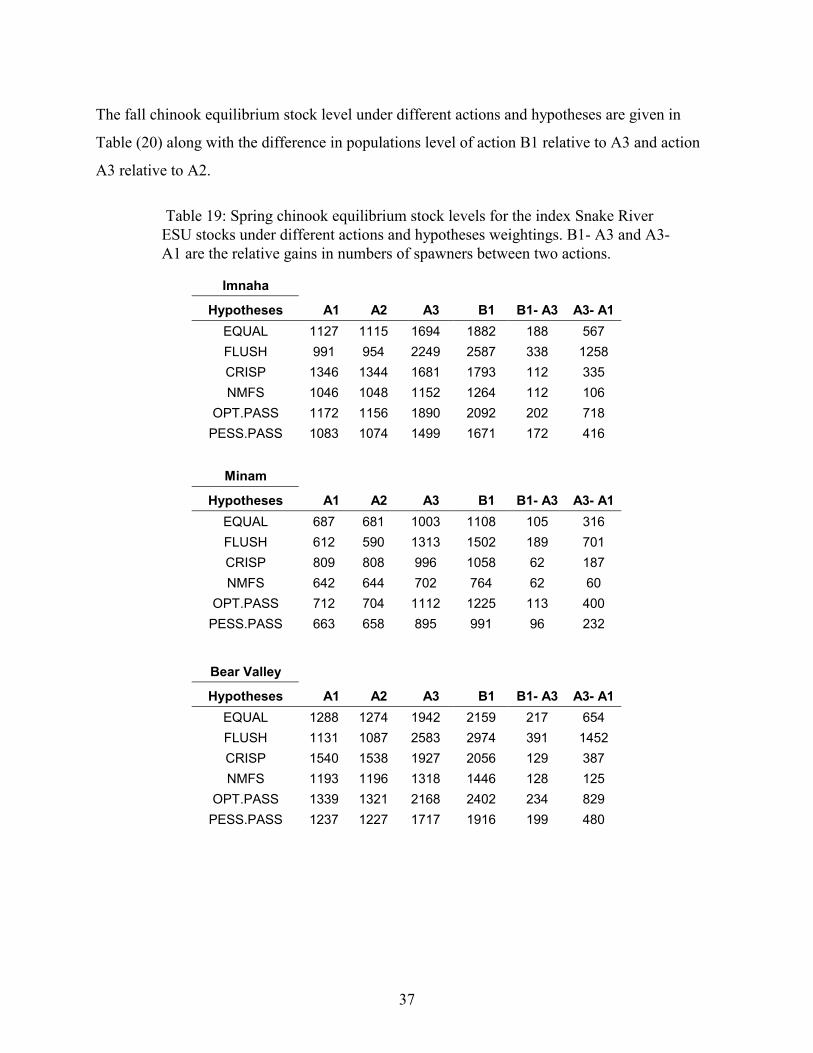
37
The fall chinook equilibrium stock level under different actions and hypotheses are given in
Table (20) along with the difference in populations level of action B1 relative to A3 and action
A3 relative to A2.
Table 19: Spring chinook equilibrium stock levels for the index Snake RiverESU stocks under different actions and hypotheses weightings. B1- A3 and A3-A1 are the relative gains in numbers of spawners between two actions.
Imnaha
Hypotheses A1 A2 A3 B1 B1- A3 A3- A1EQUAL 1127 1115 1694 1882 188 567FLUSH 991 954 2249 2587 338 1258CRISP 1346 1344 1681 1793 112 335NMFS 1046 1048 1152 1264 112 106
OPT.PASS 1172 1156 1890 2092 202 718PESS.PASS 1083 1074 1499 1671 172 416
Minam
Hypotheses A1 A2 A3 B1 B1- A3 A3- A1EQUAL 687 681 1003 1108 105 316FLUSH 612 590 1313 1502 189 701CRISP 809 808 996 1058 62 187NMFS 642 644 702 764 62 60
OPT.PASS 712 704 1112 1225 113 400PESS.PASS 663 658 895 991 96 232
Bear Valley
Hypotheses A1 A2 A3 B1 B1- A3 A3- A1EQUAL 1288 1274 1942 2159 217 654FLUSH 1131 1087 2583 2974 391 1452CRISP 1540 1538 1927 2056 129 387NMFS 1193 1196 1318 1446 128 125
OPT.PASS 1339 1321 2168 2402 234 829PESS.PASS 1237 1227 1717 1916 199 480

38
March Creek
Hypotheses A1 A2 A3 B1 B1- A3 A3- A1EQUAL 681 672 1060 1185 125 379FLUSH 590 564 1430 1656 226 840CRISP 826 826 1051 1126 75 225NMFS 626 628 698 772 74 72
OPT.PASS 711 700 1191 1325 134 480PESS.PASS 651 645 929 1044 115 278
Sulphur CR
Hypotheses A1 A2 A3 B1 B1- A3 A3- A1EQUAL 486 481 678 741 63 192FLUSH 440 426 866 980 114 426CRISP 560 559 673 711 38 113NMFS 458 458 494 532 38 36
OPT.PASS 501 495 744 813 69 243PESS.PASS 470 468 612 670 58 142
Poverty Flat
Hypotheses A1 A2 A3 B1 B1- A3 A3- A1EQUAL 1001 989 1541 1719 178 540FLUSH 871 835 2070 2391 321 1199CRISP 1208 1207 1528 1635 107 320NMFS 922 925 1025 1132 107 103
OPT.PASS 1043 1028 1727 1920 193 684PESS.PASS 958 950 1355 1519 164 397
Johnson Cr.
Hypotheses A1 A2 A3 B1 B1- A3 A3- A1EQUAL 367 363 560 623 63 193FLUSH 320 308 748 862 114 428CRISP 441 440 555 593 38 114NMFS 339 340 376 414 38 37
OPT.PASS 382 377 626 694 68 244PESS.PASS 352 349 493 552 59 141

39
Table 20: Fall chinook equilibrium stock level for the index Snake River ESUstocks under different actions and hypotheses weightings. B1- A3 and A3-A2 arethe relative gains in spawners for between two actions.
Weighting A2 A3 3yr A3 8yr B1 (10yr) B1 (15yr) B1-A3 A3-A2EQUAL 5396 15751 15326 17875 17677 2238 10143Base(-/-) 5021 15338 14913 17440 17241 2215 10105+15%/- 4876 15149 14724 17244 17049 2210 10061-15%/- 5160 15495 15067 17601 17404 2222 10121-50%/- 5628 16190 15750 18338 18137 2268 10342-75%/- 5764 16210 15781 18365 18165 2270 10232
-50%/-50% 5848 16287 15862 18437 18240 2264 10227-75%/-50% 5976 16303 15889 18460 18263 2266 10120
CRISP 4733 14938 14520 16319 16145 1503 9996FLUSH 6058 16563 16132 19430 19209 2972 10290
D1 5377 22012 21425 24641 24330 2767 16342D2 15577 23201 23077 25984 25822 2764 7562D3 2448 21638 20897 24194 23814 2737 18820D4 2718 16093 15522 18221 17982 2294 13090D5 5668 8875 8655 10463 10394 1664 3097
REGIME 6856 18543 18124 20916 20691 2470 11478BKD 6108 17192 16773 19390 19173 2299 10875
HYDRO 6108 19356 18848 21796 21540 2566 129942YR.TRAN 5396 15879 15472 18184 17963 2398 1028010YR.TRAN 5396 15622 15179 17565 17391 2078 10005LOW.EJUV 5396 14647 14293 16719 16521 2150 9074HIGH.EJUV 5396 16854 16358 19030 18833 2326 11210

40
6 Deterministic Life-cycle analysis
As an alternative to the BSM model analysis, a deterministic life-cycle model was developed to
compare the difference in performance measures between two actions. The measures are the
difference in equilibrium stock levels, the difference between maximum sustainable yield (MSY)
and the difference in MSY plus escapement. This analysis provides a relative comparison of the
merits of one action relative to another. It assumes no environmental or intrinsic variability and
as such the estimates of productivity and mortality represent long term time averages. In this
approach the environmental variations common to the pair of actions do not have to be
considered.
The deterministic model is based on the life-cycle model given by eq (1). First, number of
recruits to the spawning grounds (R) per spawner (S) is defined from eq (1) as
eq (11) R/S = P�Sm�So�Sa�H
where H is the combined ocean and in-river harvest rate. At equilibrium, the number of
spawners equals the number of recruits so R = S, and
eq (12) 1/P* = Sm�So�Sa�H
where P* is the freshwater productivity at equilibrium conditions. Applying a Ricker type density
dependence to the freshwater production term P* yields
eq (13) P* = exp(afr - b�S*)
where S* is the equilibrium spawner level and afr is the productivity component of the freshwater
life stage. Then the equilibrium stock level in terms of spawners is
eq (14) S* = (afr + log(Sm) + log(So) + log(Sa) + log(H))/b
The ratio of equilibrium freshwater productivity of two actions can be expressed
41
eq (15) Gx,y = P*y /P*x = (Smx�Sox�Sax�Hx)/(Smy�Soy�Say�Hy)
where the subscripts refer to alternatives x and y. Applying Ricker type density dependence to
the freshwater production term from eq (13) the difference in population numbers between two
alternatives is
eq (16) S*x - (by/bx)S*y = (1/bx) ln(Gx,y) + (ax - ay)/bx
Since in the hydrosystem passage corridor actions x and y are not expected to directly alter the
spawning habitat productivity rate parameters, ax = ay and bx = by, so at population equilibrium
the difference in population numbers for actions x and y is
eq (17) Ex,y = S*x - S*y = (1/b) ln(Gx,y)
The b factor is the Ricker density-dependent term, which describes how quickly the stock
productivity decreases as S increases. It can be estimated from stock recruitment data and is
insensitive to assumption to the hypotheses discussed above.
The impact of actions on the maximum sustainable yield (MSY) from a stock, Mx, under actions
x can be estimated from the intrinsic Ricker a and b parameters and the G factor given by eq (15).
No explicit function can be defined for MSY for a Ricker stock recruitment function, but M, and
the difference in MSY between actions,
eq (18) �M = Mx - My,
can be obtained numerically. Following Ricker (1978) the MSY spawning level at is obtained
from the explicit equation
eq (19) (1-bx�Smsy, x )exp(ay - b�Smsy, x ) = 1

42
The MSY for an action x is then obtained with Smsy, x in
eq (20) Mx = Smsy, x (exp(ax - bx�Smsy, x ) - 1)
where ax is the density-independent productivity term under action x. The total spawning
population under the MSY conditions is
eq (21) R = M + Smsy
The difference in R between two actions is
eq (22) �R = Rx - Ry
These MSY measures can be related to G by the equation
eq (23) ax = a0 - log G0,x
where a0 is the base, or current conditions, Ricker at term referenced to the spawning grounds
and where the Ricker term bx may or may not change between the two actions. The same
equation can be used to identify My with the substitution of parameters for action y. For the
estimation of MSY and recruitment at MSY the results are referenced to the spawning
population. Therefore, since the Ricker density independent parameter, a, given in Table 2 is
referenced to the Bonneville dam, it is related to the spawning ground term as
eq (24) a0 = a + log(SaA1)
where SaA1 is the current upriver survival of adults.

43
Because the MSY estimates depend on the Ricker a parameter as references to the base level
according to eq(23) assumptions on the distribution of factors in the base level will affect the
pairwise comparison between actions. Therefore, pairwise comparisons between actions not
involving transportation, such as A3 and B1, will depend on the assumption made on
transportation. This complication does not affect the comparisons of equilibrium levels though.
The ratio of return adults to the number of smolt outmigration (SAR) is an important measure of
the performance of the stocks. The ratio of the SAR of one action to another is in turn a relative
measure of the performance of two actions. This ratio of ratios can be expressed through Gxy.
Several measures can be defined depending on the collection point for the adults. The smolt
population is defined as the point at which the smolts enter the hydrosystem. Adults can be
defined in terms of the return to collection in the fisheries or return to the spawning ground or
hatchery. For return to the fisheries we define
eq (25) SARx/SARy = (Smx�Sox)/(Smy�Soy)
For return to the spawning grounds or hatcheries the ratio is defined
eq (26) SARx/SARy = Gx,y
The difference in equilibrium population and maximum sustainable yields can be expressed in
terms of the ratio of life stage survivals, G. The estimates of the life stage terms involve
hypotheses on how the stages are coupled and the life stage parameter values under the various
actions. In this analysis a wider range of actions are evaluated (see Table 1). Expressing
differences in equilibrium population measures in this simple analytical form illustrates the
significance of the hypotheses that come into play to produce a specific result.

44
6.1 Deterministic Life Stage Parameters
The life stage parameters used in the deterministic analysis are given in the Tables below. Four
stocks from subbasins are considered. Parameters for a representative Snake River spring
chinook are given in Table 21 and Snake River fall chinook parameters are given in Table 22.
Parameters for the Upper Columbia are given in Table 23 for Upper Columbia spring chinook
and the Hanford Reach fall chinook in Table 24. Most parameters were obtained from the PATH
analysis and are described in Section 4. Details for the Upper Columbia chinook, which were not
covered in PATH analysis, are discussed below.
The survivals of spring chinook smolts (Sm) were taken from PATH analysis as the means of
passage models. Specifically the means were taken of CRiSP with TURB 4 hypothesis and
FLUSH TURB 5 hypothesis (The results were compiled by NMFS in a spread sheet designated,
all98.xls). By taking the means of the model results a middle point estimate of direct
hydrosystem survival was obtained. In general, the CRiSP inriver passage survival estimates
were higher than the FLUSH estimates by about a factor of two. The mean CRiSP inriver
survival was about 0.44, while the FLUSH estimate was about 0.2 giving a mean of 0.32.
Although these estimates are significantly different, the direct survival estimates of transported
plus inriver passing fish are similar for the two models because most of the fish are transported
and the two models have approximately the same transport percentages and used the same direct
transport survival of 0.98.
To estimate the effect of John Day drawdown under natural river, spillway crest and natural river
with flood control the CRiSP 1.6 passage model was used (See Table 44). These CRiSP derived
estimates for the C and D actions were then adjusted to approximate the mean of Sm by adjusting
the CRiSP A1 base in river survival, designated the A1 inriver survival in Table 44) according to
the mean Sm of the A1 inriver survival estimate.
To estimate the smolt migration survival, Sm, for the Hanford Reach upriver bright fall chinook,
first the survival per kilometer of inriver passing fish was estimated from recent PIT tag studies
of fall chinook from McNary Dam to John Day Dam. The survival from MCN tailrace to BON

45
tailrace was then expressed over the travel distance plus accounting for passage at three dams.
The equation for in-river passage survival is then
eq (27) Vmcn = (dam passage survival)3 R 145.6
where R = 0.99309 is the reach survival per km and was estimated from the MCN to JDA reach
as the geometric mean of 0.53 over 76.4 km length (Smith and Achord, 1999). Using a dam
passage survival of 0.9 and a Hanford Reach (from Ringold Hatchery) to BON migration
distance of 146 km the in-river survival is Vmcn = 0.37. The PIT tag determined geometric mean
of survival from Hanford Reach to MCN dam tailrace was 0.72. Assuming that the collection
transportation survival is 1, the direct smolt passage survival can be approximated as
eq (28) Sm = Vmcn (1 - FGE) + FGE
where FGE is the fish guidance efficiency at MCN Dam. We use a representative historical
(Action A1) FGE (24%) for the base period from 1974 to 1995, which is the period over which
the parameters a and b are estimated in Schaller et al. (1999). For prospective analysis (Action
A2) we used the recent estimates of FGE = 68% (Peters et al. 1999).
The D factor for transport from McNary Dam is set at 1, which is the estimate obtained from two
methods: 1) T/C ratios and in-river survival and 2) from a life-cycle analysis (Peters et al. 1999).
To estimate the impacts of John Day drawdown we assume the drawdown survival in JDA is
0.95 and note that smolts cross 3 dams. Upstream conversion rates are taken from estimates for
the stock provided in Table 3.1.2-3 in Marmorek, Peters and Parnell (1998).
For upper Columbia spring chinook life-cycle parameter estimates, we used the Snake River
spring chinook estimates with changes reflecting the fact that these fish are not affected by the
Snake River drawdown.

46
Table 21: Snake River spring chinook survival information for the calculations.
A0 A1 A2 A3 B1 B2 B3 C1 C2 C3 D1 D2 D3 commentsSa 0.67 0.67 0.67 0.77 0.81 0.79 0.80 0.70 0.68 0.69 0.70 0.68 0.69
Sa low 0.67 0.67 0.67 0.67 0.67 0.67 0.67 0.67 0.67 0.67 0.67 0.67 0.67 lower estimateSm 0.34 0.81 0.84 0.61 0.64 0.60 0.63 0.363 0.342 0.358 0.84 0.84 0.84
�n c 0.40 0.40 0.40 0.40 0.40 0.40 0.40 0.40 0.40 0.40 0.40 0.40 0.40 bkd /climate
�n h 0.40 0.40 0.40 0.70 0.70 0.70 0.70 0.40 0.400 0.40 0.40 0.40 0.40 hydro
Pb 0.00 0.93 0.96 0.00 0.00 0.00 0.00 0.00 0.00 0.00 0.96 0.96 0.96
Table 22: Snake River fall chinook survival information for the calculations.
A0 A1 A2 A3 B1 B2 C1 C2 D1 D2 comments
Sa 0.42 0.42 0.42 0.83 0.87 0.87 0.44 0.43 0.43 0.43
Sm high 0.28 0.78 0.78 0.51 0.58 0.56 0.31 0.30 0.78 0.78 high est.
Sm low 0.28 0.78 0.78 0.35 0.40 0.39 0.31 0.30 0.78 0.78 low est.
Sm mean 0.28 0.78 0.78 0.44 0.50 0.49 0.31 0.30 0.78 0.78 mean est.
�n 1.00 1.00 1.00 1.00 1.00 1.00 1.00 1.00 1.00 1.00
Pb 0.00 0.97 0.97 0.00 0.00 0.00 0.00 0.00 0.97 0.97
Table 23: Upper Columbia spring chinook survival information for calculations.
A0 A1 A2 A3 B1 B2 B3 C1/D1 C2/D2 C3/D3
Sa 0.67 0.67 0.67 0.67 0.70 0.68 0.69 0.70 0.68 0.69
Sm 0.34 0.34 0.34 0.34 0.36 0.34 0.36 0.39 0.37 0.38
�n 1.00 1.00 1.00 1.00 1.00 1.00 1.00 1.00 1.00 1.00
Pb 0.00 0.00 0.00 0.00 0.00 0.00 0.00 0.00 0.00 0.00
Table 24: Hanford Reach fall chinook survival information for calculations.
A0 A1 A2 A3 B1 B2 C1 C2 D1/D2
Sa 0.75 0.75 0.75 0.75 0.79 0.79 0.79 0.79 0.79
Sm 0.31 0.31 0.54 0.19 0.21 0.20 0.21 0.20 0.54
�n 1.00 1.00 1.00 1.00 1.00 1.00 1.00 1.00 1.00
Pb 0.00 0.55 0.89 0.00 0.00 0.00 0.00 0.00 0.89

47
6.2 Equations for comparison of actions
6.2.1 Equilibrium Population and MSY Differences in Drawdown Actions
The pairwise difference between actions x and y equilibrium populations, Ex,y, described by eq
(17) and the maximum sustained yield �Mx,y using eq (19), eq (20) and eq (23), both use Gx,y
from eq (15). For John Day drawdown actions relative to Snake River drawdown the growth ratio
equation reduces to
eq (29) Gx,A3 = (Sax/SaA3)(Smx /SmA3)
where the actions are x = B1, B2, B3, C1, C2, C3 as detailed in Table 1, and the adult and smolt
migration survival values are given in Table 21 and 22. In these calculations the ocean survival
factors are assumed equal under all alternatives. That is, the effects of hydrosystem passage under
Snake River drawdown, (A3), the Snake and John Day (B1, B2, B3) and a John Day drawdown
only (C1, C2, C3) are set equal, so the ratio of post-Bonneville survivals, �nx/�ny, is always 1.
6.2.2 Equilibrium and MSY Differences of Transport vs. Drawdown Actions
For comparing transportation and drawdown actions the population growth index for spring
chinook takes the form
eq (30) GA1,y = [SaA1/Say][(DA1PbA1+1-PbA1)][�nA1/�ny][SmA1/Smy]
The difference in equilibrium populations between A1 and alternative y is estimated by using
GA1,y in eq (17) and the difference in MSY is estimated with eq (19), eq (20) and eq (23).
The for comparing transportation to drawdown actions population growth index for Snake River
fall chinook is calculated by the equation
eq (31) GA1,y = [SaA1/Say][(DA1�PbA1+1-PbA1)][SmA1/Smy].
48
Here the ocean survival term under actions A1 and y are assumed equal. This result comes from
the PATH fall chinook retrospective analysis, which indicated that under low levels of D that
extra mortality was negligible. That is, under an assumption of low D, the decline in the fall
chinook is principally the result of their transportation. The result does not hold if D is high
though. Then an extra mortality term is required to account for the decline in the fall chinook. In
this case eq (31) is still appropriate under CLIMATE and BKD hypotheses. The description of
the extra mortality for fall chinook, thus, has not been resolved. This issue is not critical when
evaluating the impact of the addition of a John Day drawdown, since ocean survival under this
action is not expected to be significantly different from ocean survival under a drawdown of both
the Snake River system and John Day.
6.2.3 Equivalence points
An important consideration is the mix of life-stage survivals that make drawdown and
transportation actions equivalent in terms of the equilibrium population levels. Note that the
different drawdown actions are always different in that additional drawdown produces higher
survival under the assumptions of this analysis. The equivalence point at which A2 and A3 given
equal population levels can be expressed by setting GA2,A3 = 1. The resulting equivalence point
between transportation and drawdown for Snake River spring chinook is
eq (32) SaA3�SmA3 = DA2��nA2 / �ny / 2
where the factor 1/2 is approximately the product of smolt and adult upstream survivals in the
existing system. The Snake River fall chinook equivalence point between transportation and
drawdown actions is
eq (33) SaA3�SmA3 ~ DA2/3
where the factor 1/3 is the approximate product of the smolt and adult river migration survival
under the existing passage conditions.
49
6.3 Results
6.3.1 Pairwise comparison of drawdown alternatives
The typical equilibrium population of an index stock under action A1 is 419 for spring chinook
and 7259 for fall chinook. The resulting difference in spawners at population equilibrium and
MSY for a pairwise comparison of drawdown alternatives is given in Tables 25 and 26 for Snake
River spring chinook and in Tables 27 and 28 for Snake River fall chinook. For example,
comparing action A3 to action B1 in Table 25, at equilibrium, action B1 results in 58 more
spawners than action A3. These estimates are based on b given in Table (2). The number of
spring chinook stocks in the Snake River Basin is on the order of 38 making a total equilibrium
population of about 16000. Thus we expect a 58x38 = 2204 fish increase in the Snake River
Basin index spawning population by including the John Day drawdown with a Snake River
drawdown action (B1). For fall chinook, the equilibrium population size in the Snake River
basin is about 7000 making the maximum benefit of a John Day action in addition to a Snake
River drawdown of about 650 spawners. For the fall chinook analysis, the effect of uncertainties
in the smolt survival with Snake River drawdown are illustrated by providing equilibrium levels
and MSY for high and low smolt survivals (Tables 27 and 28).
The �M estimates in Table 26 depends on the assumption on D. To a good approximation the
relationship is linear with �M decreasing as D increases. For a comparison of A3 to B1 the
influence in D can be expressed by the equation
eq (34) �MA3,B1 = 157 – 147 D

50
Table 25: Spring chinook equilibrium population differences Erow,col. Equilibriumnumber of spring chinook under A1 is 420 fish per stock.
B1 B2 B3 C1 C2 C3
A3 56 5 40 -354 -404 -370
B1 0 -52 -17 -410 -461 -427
B2 0 35 -359 -410 -375
B3 0 -394 -445 -410
C1 0 -51 -17
C2 0 34
Table 26: Spring chinook MSY difference population differences �Mrow,col).MSY for spring chinook under A1 is 93 fish per stock.
B1 B2 B3 C1 C2 C3
A3 108 10 76 -448 -488 -461
B1 0 -98 -32 -556 -596 -569
B2 0 66 -458 -498 -471
B3 0 -524 -564 -537
C1 0 -40 -13
C2 0 27
Table 26a: Snake River spring chinook G row,col.
B1 B2 B3 C1 C2 C3
A3 1.1 1.00 1.07 0.54 0.49 0.52
B1 1.0 0.91 0.97 0.49 0.44 0.47
B2 1.00 1.06 0.53 0.49 0.52
B3 1.00 0.50 0.46 0.49
C1 1.00 0.91 0.97
C2 1.00 1.06

51
Table 27: Snake river fall chinook equilibrium population differences Erow,colunder high (0.9) and low (0.6) estimates of free-flowing river smolt survivalVl. Equilibrium number of fall chinook under A1 is 7259 fish.
VlA3 B1 B2 C1 C2
A3 0.9 650 520 -4195 -4401
B1 0.9 -130 -4846 -5052
B2 0.9 -4716 -4922
C1 0.9 -207
A3 0.6 668 575 -2801 -3007
B1 0.6 -94 -3469 -3676
B2 0.6 -3376 -3582
C1 0.6 -207
Table 28: Snake River fall chinook differences in MSY population�Mrow,col under high (0.9) and low (0.6) estimates of free-flowing riversmolt survival Vl. MSY for fall chinook under A1 is 6548 fish.
VlA3 B1 B2 C1 C2
A3 0.9 12828 10082 -45136 -46290
B1 0.9 -2746 -57964 -59118
B2 0.9 -55218 -56372
C1 0.9 -1154
A3 0.6 9061 7690 -24199 -25353
B1 0.6 -1371 -33260 -34414
B2 0.6 -31889 -33043
C1 0.6 -1154
Table 28a: Snake River fall chinook G row,col with Sm set as the
average of high and low estimates from Table 22.
B1 B2 C1 C2
A3 1.19 1.16 0.37 0.35
B1 1.00 0.98 0.31 0.29
B2 1.00 0.31 0.30
C1 1.00 0.94

52
6.3.2 Pairwise comparison of transport vs. drawdown alternatives
Differences in equilibrium and MSY populations for Snake River and Upper Columbia stocks,
for drawdown actions relative to the current operations conditions, A1, are illustrated in Tables
29 through 37. Positive values indicate the alternative action population is above the level from
A1 population. Upper and lower estimates of the population level are illustrated for different
assumptions on ocean survival and adult migration conversion rates. Also illustrated are the
impacts of the three levels of D for spring chinook (see Table 6 for description) and fall chinook
(see Table 7 for description).
For a Snake River spring chinook index stock, G is defined by eq (30). The life-cycle parameter
values are given in Table 21, and the results are given in Tables 29, 30, 31, 31a and 33. The
greatest increase above A1 occurs for B1 (828 spawners for E) under a low transportation
efficiency in A1 (D = 0.35), and in changing from A1 to B1, the ocean survival increases by the
factor 1.75 and adult upstream conversion (survival) increases by 1.15 (Table 29). If upstream
conversion and ocean survival do not increase between A1 and B1 and transportation is effective,
as expressed by D = 0.8, then changing from A1 to B1 causes a decreases in the equilibrium level
by 18 spawners under equilibrium E. In Table 32 the effect of C actions are not computed for an
increase in ocean survival because a drawdown of John Day reservoir without drawing down the
Snake River reservoirs is not expected to increase ocean survival.
For a Snake River fall chinook index stock G is defined by eq (31). The life-cycle parameter
values are given in Table 22. Pairwise comparisons of actions are given in Tables 31a, 33a, 34
and 34a, 35, 36 and 37. Comparing the effect of transportation, A1, with putting fish back in the
river with no transportation, action A0, is illustrated in Table 33a. A0 is a preferred option
except when transportation effectiveness is high (D = 1). Also, improving transportation,
represented by DA2, also improves fish stocks. Here, only the D hypotheses are a major
determinant of the difference between A2 and A0. The balance between D and the passage
survivals is illustrated in eq (33), showing the equivalence point where drawdown and
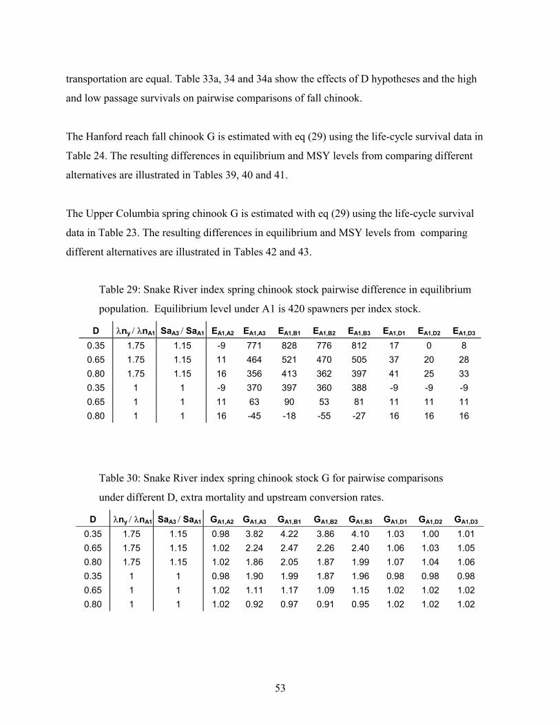
53
transportation are equal. Table 33a, 34 and 34a show the effects of D hypotheses and the high
and low passage survivals on pairwise comparisons of fall chinook.
The Hanford reach fall chinook G is estimated with eq (29) using the life-cycle survival data in
Table 24. The resulting differences in equilibrium and MSY levels from comparing different
alternatives are illustrated in Tables 39, 40 and 41.
The Upper Columbia spring chinook G is estimated with eq (29) using the life-cycle survival
data in Table 23. The resulting differences in equilibrium and MSY levels from comparing
different alternatives are illustrated in Tables 42 and 43.
Table 29: Snake River index spring chinook stock pairwise difference in equilibrium
population. Equilibrium level under A1 is 420 spawners per index stock.
D ��ny ���nA1 SaA3 ��SaA1 EA1,A2 EA1,A3 EA1,B1 EA1,B2 EA1,B3 EA1,D1 EA1,D2 EA1,D3
0.35 1.75 1.15 -9 771 828 776 812 17 0 80.65 1.75 1.15 11 464 521 470 505 37 20 280.80 1.75 1.15 16 356 413 362 397 41 25 330.35 1 1 -9 370 397 360 388 -9 -9 -90.65 1 1 11 63 90 53 81 11 11 110.80 1 1 16 -45 -18 -55 -27 16 16 16
Table 30: Snake River index spring chinook stock G for pairwise comparisons
under different D, extra mortality and upstream conversion rates.
D ��ny ���nA1 SaA3 ��SaA1 GA1,A2 GA1,A3 GA1,B1 GA1,B2 GA1,B3 GA1,D1 GA1,D2 GA1,D3
0.35 1.75 1.15 0.98 3.82 4.22 3.86 4.10 1.03 1.00 1.010.65 1.75 1.15 1.02 2.24 2.47 2.26 2.40 1.06 1.03 1.050.80 1.75 1.15 1.02 1.86 2.05 1.87 1.99 1.07 1.04 1.060.35 1 1 0.98 1.90 1.99 1.87 1.96 0.98 0.98 0.980.65 1 1 1.02 1.11 1.17 1.09 1.15 1.02 1.02 1.020.80 1 1 1.02 0.92 0.97 0.91 0.95 1.02 1.02 1.02

54
Table 31: Snake River index spring chinook stock differences in maximumsustainable yield pairwise comparisons of actions.�
D ��ny ���nA1 SaA3 ��SaA1 �MA1,A2 �MA1,A3 �MA1,B1 �M A1,B2 �MA1,B3 �MA1,D1 �MA1,D2 �MA1,D3
0.35 1.75 1.15 -1 648 756 658 724 4 1 20.65 1.75 1.15 3 241 297 245 280 8 5 60.80 1.75 1.15 4 152 196 156 183 9 6 70.35 1 1 -1 162 183 155 176 -1 -1 -10.65 1 1 3 15 22 12 20 3 3 30.80 1 1 4 -7 -3 -8 -4 4 4 4
Table 31a: Snake River index fall chinook stock differences �R pairwisecomparisons of actions.�
D ��ny ���nA1 SaA3 ��SaA1 �RA1,A2 �RA1,A3 �RA1,B1 �R A1,B2 �RA1,B3 �RA1,D1 �RA1,D2 �RA1,D3
0.35 1.75 1.15 -5 927 1049 938 1013 11 0 60.65 1.75 1.15 8 426 502 433 479 25 14 190.80 1.75 1.15 11 300 364 305 345 28 17 220.35 1 1 -5 314 345 304 335 -5 -5 -50.65 1 1 8 43 63 36 56 8 8 80.80 1 1 11 -28 -11 -33 -16 11 11 11
Table 32: Snake River index stock spring chinook levels for E, �M, G, and �Runder different levels of D for comparison of A1 to the C alternatives. Note thatwith John Day Drawdown no benefit on ocean survival is assumed to occur.
D EA1,C1 EA1,C2 EA1,C3 �MA1,C1 �MA1,C2 �MA1,C3 GA1,C1 GA1,C2 GA1,C3 �RA1,C1 �RA1,C2 �RA1,C3
0.35 96 46 80 24 10 19 1.18 1.08 1.15 67 31 550.65 -210 -261 -227 -16 -14 -16 0.69 0.63 0.67 -118 -142 -1250.80 -318 -369 -335 -10 -4 -8 0.57 0.52 0.55 -167 -188 -174
Table 33: Snake River spring chinook difference in equilibrium E, maximumsustainable yield��M, and total population under MSY��R under different Dhypotheses
D EA1,A0 EA1,A2 ���MA1,A0 �MA1,A2 �RA1,A0 �RA1,A2
0.35 35 -9 8 -1 23 -5
0.65 -272 11 -14 3 -147 80.80 -380 16 -2 4 -192 11

55
Table 33a: Snake River fall chinook difference in equilibrium E, maximumsustainable yield��M, and total population under MSY��R under different Dhypotheses
D A1 D A2 EA1,A0 EA1,A2 ���MA1,A0 �MA1,A2 �RA1,A0 �R A1,A2
0.05 0.24 5631 4475 13700 8827 15054 99950.05 1.00 5631 9424 13700 46673 15054 484040.05 0.05 5631 0 13700 0 15054 00.20 0.20 1747 0 2103 0 2650 01.00 1.00 -3794 0 -1499 0 -3099 0
Table 34: Snake River fall chinook difference in equilibrium populations for passagesurvivals and D assumptions. Note equilibrium population under A1 is 7259 spawners.
Passage DA1 EA1,A3 EA1,B1 EA1,B2 EA1,D1 EA1,D2
0.05 10373 11024 10894 172 87 0.20 6490 7141 7011 172 87SaA3 high
SmA3 high 1.00 949 1599 1469 172 87
0.05 6456 6951 6857 0 0 0.20 2573 3067 2973 0 0
SaA3 low
SmA3 low 1.00 -2969 -2474 -2568 0 0
Table 34a: Snake River fall chinook difference in �R for passage survivals and Dassumptions.
Passage DA1 �R A1,A3 �R A1,B1 �R A1,B2 �R A1,D1 �R A1,D2
0.05 63548 76406 73654 214 107 0.20 19963 24498 23528 214 107SaA3 high
SmA3 high 1.00 1300 2381 2151 214 107
0.05 19749 24365 23665 214 107 0.20 4364 6033 5781 214 107
SaA3 low
SmA3 low 1.00 -2625 -2177 -2244 214 107

56
Table 35: Snake River fall chinook difference in maximum sustained yield for
different passage survivals and D assumptions.
Passage DA1 ��MA1,A3 �MA1,B1 �MA1,B2 �MA1,D1 �MA1,D2
0.05 61764 74592 71846 155 77 0.20 18494 22955 21999 155 77SaA3 high
SmA3 high 1.00 987 1876 1683 155 77
0.05 18284 22824 22135 155 77 0.20 3600 5113 4881 155 77SaA3 low
SmA3 low 1.00 -1419 -1271 -1297 155 77
Table 36: Snake River fall chinook G for passage survivals and D assumptions.
Passage DA1 GA1,A3 GA1,B1 GA1,B2 GA1,D1 GA1,D2
0.05 16.46 19.62 18.94 1.04 1.02 0.20 5.76 6.87 6.63 1.04 1.02SaA3 high
SmA3 high 1.00 1.29 1.54 1.48 1.04 1.02
0.05 5.71 6.53 6.36 1.00 1.00 0.20 2.00 2.28 2.23 1.00 1.00SaA3 low
SmA3 low 1.00 0.44 0.51 0.50 1.00 1.00
Table 37: Snake River fall chinook levels for E, �M and G under different levelsof D and passage survivals for comparison of A1 to the C alternatives.
Passage DA1 EA1,C1 EA1,C2 �MA1,C1 �MA1,C2 GA1,C1 GA1,C2 �R A1,C1 �R A1,C2
0.05 6179 5972 16628 15474 5.30 5.01 18058 16877 0.20 2295 2089 3055 2678 1.85 1.75 3749 3318SaA3 high
SmA3 high 1.00 -3246 -3452 -1458 -1479 0.41 0.39 -2793 -2912
0.05 6179 5972 16628 15474 5.30 5.01 18058 15877 0.20 2295 2089 3055 2678 1.85 1.75 2749 3318SaA3 low
SmA3 low 1.00 -3246 -3452 -1458 -1479 0.41 0.39 -2793 -2912
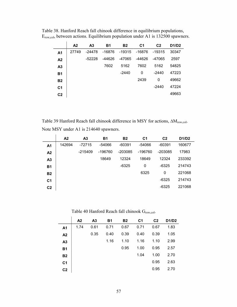
57
Table 38. Hanford Reach fall chinook difference in equilibrium populations,Erow,col, between actions. Equilibrium population under A1 is 132500 spawners.
A2 A3 B1 B2 C1 C2 D1/D2
A1 27749 -24478 -16876 -19315 -16876 -19315 30347
A2 -52228 -44626 -47065 -44626 -47065 2597
A3 7602 5162 7602 5162 54825
B1 -2440 0 -2440 47223
B2 2439 0 49662
C1 -2440 47224
C2 49663
Table 39 Hanford Reach fall chinook difference in MSY for actions, �Mrow,col.
Note MSY under A1 is 214640 spawners.
A2 A3 B1 B2 C1 C2 D1/D2
A1 142694 -72715 -54066 -60391 -54066 -60391 160677
A2 -215409 -196760 -203085 -196760 -203085 17983
A3 18649 12324 18649 12324 233392
B1 -6325 0 -6325 214743
B2 6325 0 221068
C1 -6325 214743
C2 -6325 221068
Table 40 Hanford Reach fall chinook Grow,col.
A2 A3 B1 B2 C1 C2 D1/D2
A1 1.74 0.61 0.71 0.67 0.71 0.67 1.83
A2 0.35 0.40 0.39 0.40 0.39 1.05
A3 1.16 1.10 1.16 1.10 2.99
B1 0.95 1.00 0.95 2.57
B2 1.04 1.00 2.70
C1 0.95 2.63
C2 0.95 2.70
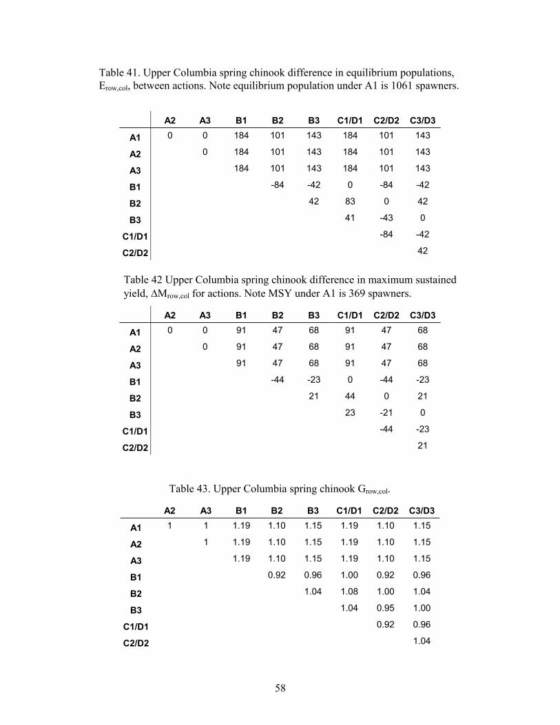
58
Table 41. Upper Columbia spring chinook difference in equilibrium populations,Erow,col, between actions. Note equilibrium population under A1 is 1061 spawners.
A2 A3 B1 B2 B3 C1/D1 C2/D2 C3/D3
A1 0 0 184 101 143 184 101 143
A2 0 184 101 143 184 101 143
A3 184 101 143 184 101 143
B1 -84 -42 0 -84 -42
B2 42 83 0 42
B3 41 -43 0
C1/D1 -84 -42
C2/D2 42
Table 42 Upper Columbia spring chinook difference in maximum sustainedyield, �Mrow,col for actions. Note MSY under A1 is 369 spawners.
A2 A3 B1 B2 B3 C1/D1 C2/D2 C3/D3
A1 0 0 91 47 68 91 47 68
A2 0 91 47 68 91 47 68
A3 91 47 68 91 47 68
B1 -44 -23 0 -44 -23
B2 21 44 0 21
B3 23 -21 0
C1/D1 -44 -23
C2/D2 21
Table 43. Upper Columbia spring chinook Grow,col.
A2 A3 B1 B2 B3 C1/D1 C2/D2 C3/D3
A1 1 1 1.19 1.10 1.15 1.19 1.10 1.15
A2 1 1.19 1.10 1.15 1.19 1.10 1.15
A3 1.19 1.10 1.15 1.19 1.10 1.15
B1 0.92 0.96 1.00 0.92 0.96
B2 1.04 1.08 1.00 1.04
B3 1.04 0.95 1.00
C1/D1 0.92 0.96
C2/D2 1.04

59
7 Downstream passage model
The CRiSP model (Anderson et al. 1999) was used for the detailed analysis of actions at the John
Day project. The model tracks release groups of juvenile salmonids as they migrate through the
hydrosystem. Mortality is attributed to direct dam mortality (as fish pass through the turbines,
bypass, or spillways of dams), predation (in the forebays, tailraces and main reservoirs), and gas
bubble disease resulting from nitrogen supersaturation. Fish migration rate is modeled in terms of
river velocity date in the season, and length of time in migration (Zabel and Anderson 1997,
Zabel et al. 1998). In addition, fish are collected at several dams and transported to below
Bonneville Dam.
For the life-cycle modeling, a combination of CRiSP v1.5 and v1.6 was utilized. CRiSP v1.5 was
used in the PATH spring chinook analysis, and the results from these runs were used in the life-
cycle analysis, with the following exception. For the more detailed analysis of explicit actions at
the John Day project (results presented below) we utilized CRiSP v1.6. The previous v1.5 results
were then scaled to reflect the proportional survival increases under the various actions. CRiSP
v1.6 was used for all fall chinook analyses since this was the version used in PATH.
The primary difference between v1.5 and v1.6 is the data used for survival calibration. CRiSP
v1.6 relies on NMFS survival estimates from PIT tag data (details in Anderson et al. 1999).
CRiSP v1.5 was calibrated to predator consumption and abundance indices (Anderson et al.
1996). Comparisons between the two versions show that they produce similar results. All dam
passage parameters (FGE, spill effectiveness, dam passage mortality) for both versions were
taken from PATH reports (e.g., Marmorek et al. 1998) and were common to both CRiSP and
FLUSH models.
7.1 Configuration for John Day drawdown
For spring chinook, survival through John Day was modeled with both reservoir improvement
and John Day Dam passage improvements. Reservoir survival was modeled to reflect a decrease

60
in reservoir passage time resulting from the increased water velocity through the reservoir. In
natural river drawdown, John Day Dam passage survival was set at 100%. With spillway crest
drawdown, passage survival was set at 98%.
For fall chinook, upper and lower bounds were modeled for John Day drawdown. Both bounds
assumed that with natural drawdown the survival in dam passage and the forebay would be
removed. An upper bound of reservoir survival was modeled to increase in proportion with the
increase in water velocity, which reflects a decrease in reservoir residence. For a lower bound the
fish travel time was not decreased with drawdown. For spillway crest drawdown these same
scenarios were applied for reservoir survival but dam passage survival was set to 98% reflecting
a small mortality in spillway passage.
7.2 Passage Model Results
For CRiSP model runs presented in this analysis, fish were released at the forebay of Lower
Granite Dam. The release distributions were based on passage index data for wild spring and fall
chinook. Survivals and travel times were computed from release point to Bonneville tailrace. The
survivals reported were a weighted average based on release size. The travel times were the
median travel times for all fish in a given year.
The model runs utilized historical flows and temperatures with current dam operations and
survivals. Water years modeled, including flow and temperature conditions, were 1975-1998 for
spring chinook and 1975-1992 for fall chinook.
7.2.1 Mortality associated with the John Day project
The improvement in survival as a result of an action at the John Day project can be calculated as
eq (35) �S = SY/ SX – 1.0

61
where SX is the total in-river survival with John Day project at full pool and SY is the total in-
river survival under an action X at John Day projects. This can be expressed as a percentage by
multiplying the result by 100.
7.2.2 Changes in travel time under John Day operations
The change in travel time associated with different John Day operations can be expressed
eq (36) �tt = ttX – ttX
where ttX is the travel time through John Day reservoir with full pool operation and ttY is the
travel time through John Day pool under various actions.
7.2.3 Spring Chinook Results
The results of the spring chinook passage modeling analysis are presented in Tables 44 to 47.
The flood control scenario was performed for 1997 only, which was a high flow year.
Table 44: In-river survival for Snake River spring chinook under variousmanagement actions. Survivals are from the forebay of Lower Granite Dam to thetailrace of Bonneville Dam. High survival uses drawdown survival through SnakeRiver of 0.95, low survival used drawdown survival of 0.85.
min mean max S.D.A1 (inriver only) 0.327 0.437 0.551 0.062
A3 (high survival) 0.533 0.619 0.719 0.042A3 (low survival) 0.477 0.554 0.635 0.038B1 (high survival) 0.640 0.705 0.777 0.042B1 (low survival) 0.570 0.631 0.695 0.038
C1 (JD draw down) 0.391 0.498 0.603 0.062C2 (JD spill crest) 0.360 0.471 0.580 0.064
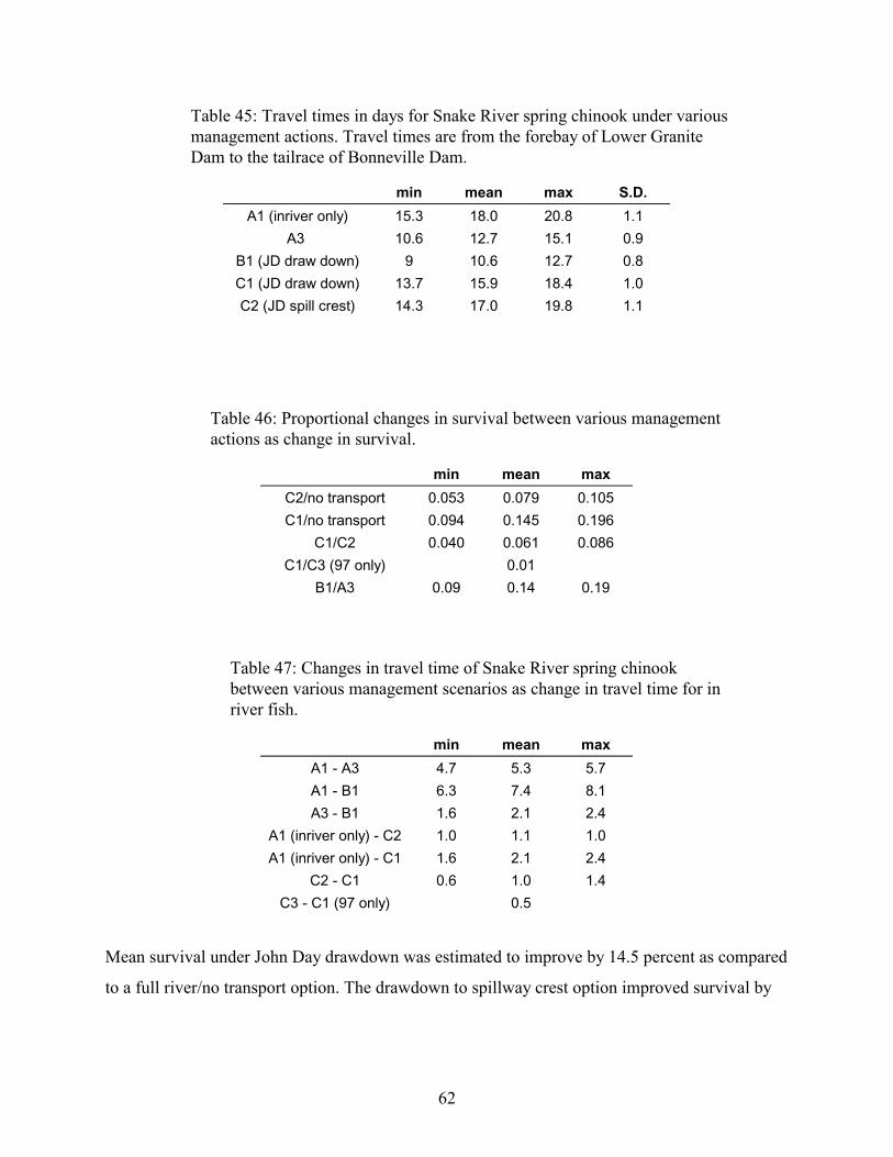
62
Table 45: Travel times in days for Snake River spring chinook under variousmanagement actions. Travel times are from the forebay of Lower GraniteDam to the tailrace of Bonneville Dam.
min mean max S.D.A1 (inriver only) 15.3 18.0 20.8 1.1
A3 10.6 12.7 15.1 0.9B1 (JD draw down) 9 10.6 12.7 0.8C1 (JD draw down) 13.7 15.9 18.4 1.0C2 (JD spill crest) 14.3 17.0 19.8 1.1
Table 46: Proportional changes in survival between various managementactions as change in survival.
min mean maxC2/no transport 0.053 0.079 0.105C1/no transport 0.094 0.145 0.196
C1/C2 0.040 0.061 0.086C1/C3 (97 only) 0.01
B1/A3 0.09 0.14 0.19
Table 47: Changes in travel time of Snake River spring chinookbetween various management scenarios as change in travel time for inriver fish.
min mean maxA1 - A3 4.7 5.3 5.7A1 - B1 6.3 7.4 8.1A3 - B1 1.6 2.1 2.4
A1 (inriver only) - C2 1.0 1.1 1.0A1 (inriver only) - C1 1.6 2.1 2.4
C2 - C1 0.6 1.0 1.4C3 - C1 (97 only) 0.5
Mean survival under John Day drawdown was estimated to improve by 14.5 percent as compared
to a full river/no transport option. The drawdown to spillway crest option improved survival by
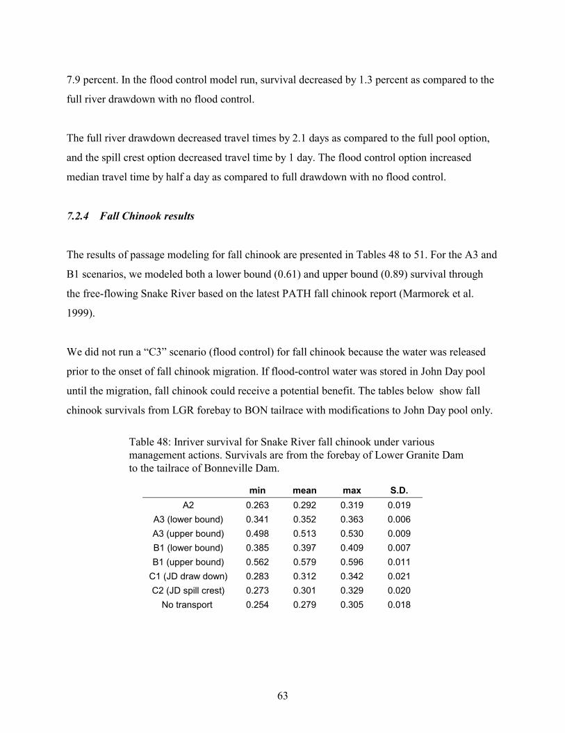
63
7.9 percent. In the flood control model run, survival decreased by 1.3 percent as compared to the
full river drawdown with no flood control.
The full river drawdown decreased travel times by 2.1 days as compared to the full pool option,
and the spill crest option decreased travel time by 1 day. The flood control option increased
median travel time by half a day as compared to full drawdown with no flood control.
7.2.4 Fall Chinook results
The results of passage modeling for fall chinook are presented in Tables 48 to 51. For the A3 and
B1 scenarios, we modeled both a lower bound (0.61) and upper bound (0.89) survival through
the free-flowing Snake River based on the latest PATH fall chinook report (Marmorek et al.
1999).
We did not run a “C3” scenario (flood control) for fall chinook because the water was released
prior to the onset of fall chinook migration. If flood-control water was stored in John Day pool
until the migration, fall chinook could receive a potential benefit. The tables below show fall
chinook survivals from LGR forebay to BON tailrace with modifications to John Day pool only.
Table 48: Inriver survival for Snake River fall chinook under variousmanagement actions. Survivals are from the forebay of Lower Granite Damto the tailrace of Bonneville Dam.
min mean max S.D.A2 0.263 0.292 0.319 0.019
A3 (lower bound) 0.341 0.352 0.363 0.006A3 (upper bound) 0.498 0.513 0.530 0.009B1 (lower bound) 0.385 0.397 0.409 0.007B1 (upper bound) 0.562 0.579 0.596 0.011
C1 (JD draw down) 0.283 0.312 0.342 0.021C2 (JD spill crest) 0.273 0.301 0.329 0.020
No transport 0.254 0.279 0.305 0.018
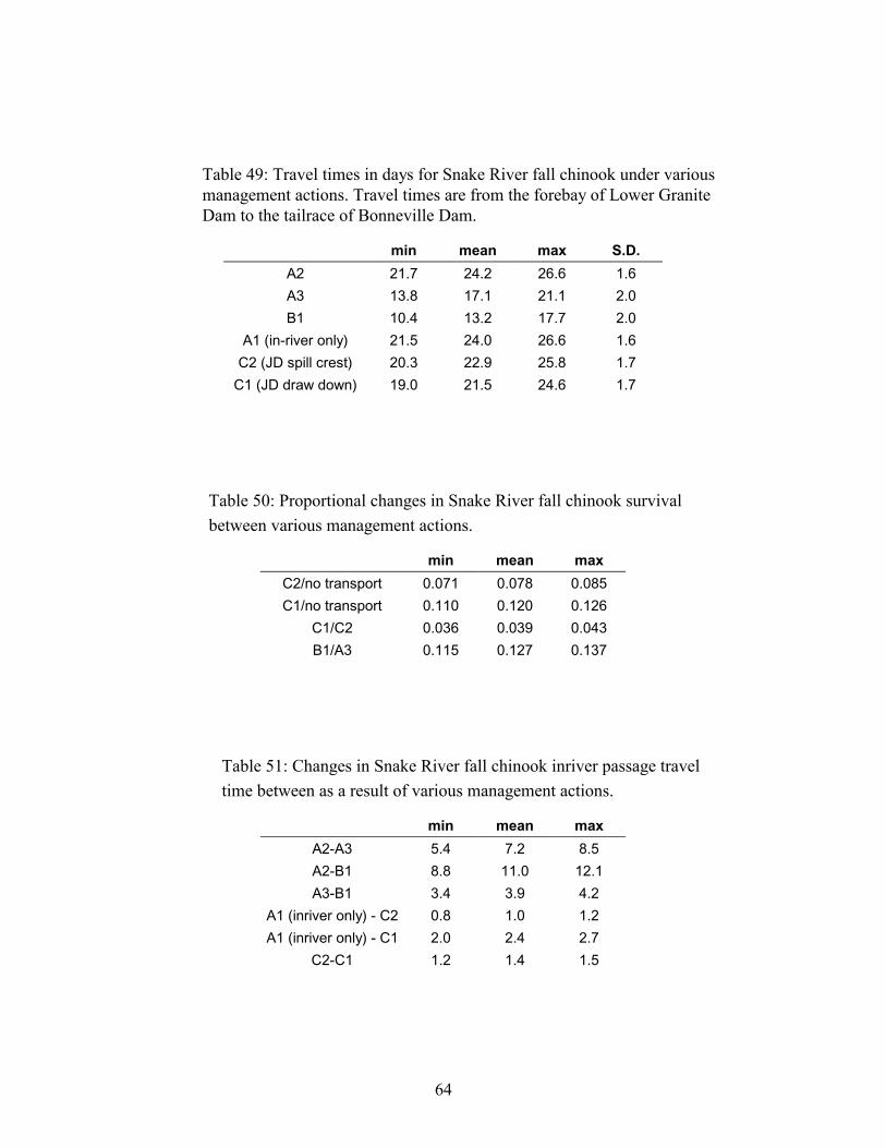
64
Table 49: Travel times in days for Snake River fall chinook under variousmanagement actions. Travel times are from the forebay of Lower GraniteDam to the tailrace of Bonneville Dam.
min mean max S.D.A2 21.7 24.2 26.6 1.6A3 13.8 17.1 21.1 2.0B1 10.4 13.2 17.7 2.0
A1 (in-river only) 21.5 24.0 26.6 1.6C2 (JD spill crest) 20.3 22.9 25.8 1.7
C1 (JD draw down) 19.0 21.5 24.6 1.7
Table 50: Proportional changes in Snake River fall chinook survivalbetween various management actions.
min mean maxC2/no transport 0.071 0.078 0.085C1/no transport 0.110 0.120 0.126
C1/C2 0.036 0.039 0.043B1/A3 0.115 0.127 0.137
Table 51: Changes in Snake River fall chinook inriver passage traveltime between as a result of various management actions.
min mean maxA2-A3 5.4 7.2 8.5A2-B1 8.8 11.0 12.1A3-B1 3.4 3.9 4.2
A1 (inriver only) - C2 0.8 1.0 1.2A1 (inriver only) - C1 2.0 2.4 2.7
C2-C1 1.2 1.4 1.5
65
The improvement in survival conferred by drawing down John Day pool to a natural river level
as compared to full pool operations is estimated to be 12-13 per cent. This is based on comparing
survival under A3 (drawdown of all four Snake River projects) to B1 (drawdown of Snake
projects and John Day) and by comparing C1 (John Day drawdown only) to the full river/no
transport option. Note that this improvement in survival results from both reduced reservoir and
dam mortality. Approximately 2/3 of this improvement could be realized by only drawing the
river down to the spill crest level.
Travel times were reduced by 2-4 days with John Day drawdown.
8 Discussion
The impact of John Day drawdown action on the Snake River and Upper Columbia spring and
fall chinook was evaluated using several response measures and three modeling approaches. The
analysis was conducted with the PATH Bayesian life-cycle analysis, which provided probabilities
of meeting survival and recovery goals. In addition, the analysis was applied to determine the
equilibrium spawner levels. This analysis was conducted for Snake River listed spring and fall
chinook. A second approach used a deterministic life-cycle analysis under equilibrium
conditions. This approach provided the equilibrium number of spawners, the MSY and the total
adult population under MSY of Snake River spring and fall chinook, Hanford Reach fall
chinook, and Upper Columbia spring chinook. A third analysis evaluated the impact of the
drawdown actions on the smolt passage survival and travel time using the CRiSP smolt passage
model.
Actions evaluated include transportation, Snake drawdown only, John Day drawdown only, with
and without transportation from the Snake River, and a drawdown including the Snake River and
John Day reservoir. Three variations of John Day drawdown were evaluated: natural river
drawdown, spillway crest drawdown, and natural river drawdown with flood control measures in
the spring that allowed for partial refilling of the reservoir during times of high flow.

66
Six of stock performance measures were evaluated: probability of survival over 24 years,
probability of recovery over 48 years, equilibrium population level, maximum sustainable yields,
smolt passage survival, and smolt passage travel time. A number of hypotheses were explored on
in-river survival of smolts and the linkages between freshwater survival, smolt passage stages,
and ocean survival. In addition, several hypotheses were explored on the expected levels of
survival under drawdown and on the survival of adults migrating up river.
The Bayesian analysis and the deterministic analysis both provide pairwise estimates of the
difference in equilibrium population levels between two alternatives. The Bayesian results for
Snake River spring chinook are given in Table 19 and the deterministic results are given in Table
25. The Bayesian analysis gave larger values. For example, the difference in equilibrium
population levels between alternatives B1 and A3 for the Bayesian analysis were between 68 and
217 spawners under equal weighting of hypotheses, while the deterministic value was 58.
Although these estimates are different the ratio of the equilibrium levels defined (B1-A3)/A1 is
nearly identical for the two methods. From the Bayesian analysis (Table 19) the geometric mean
of this ratio, across the 7 index stocks, is 0.163. For the deterministic model the ratio is 0.138.
Noting from eq (17) that the equilibrium level in the deterministic model is scaled by the Ricker
parameter b, it follows that the value of a pairwise comparison depends on b, but in the ratio
measure, (B1-A3)/A1, the Ricker b terms cancel. This is also true of the Bayesian model.
We note that the equilibrium ratio (B1-A3)/A1 is very close in the two methods while the
measure B1-A3 is different. Therefore, the main difference in pairwise comparisons from the two
methods involves the choice of the Ricker b used in each method. For the Bayesian analysis the
mean value of the Ricker b is 0.00122 while the mean value for the deterministic method was
0.00174. The difference in the estimates of b accounts for over 80% of the difference in the
results of the two methods. The remaining difference in the methods is a result of slightly
different passage assumptions. Mathematically the two approaches are functionally equivalent, so
using the same input in the two methods should give very similar results.
67
The question of which set of Ricker b estimates are better can not be resolved. In this work the
estimates used in the Bayesian analysis and the estimates used in the deterministic method were
both extracted from work by the same researchers developed at different times. The Bayesian
analysis used b values prepared by Schaller, Petrosky and Langness for the PATH analysis
(Marmorek and Peters 1998) and the deterministic estimate used b values published by Schaller
et al (1999).
8.1 Bayesian Analysis
The analysis showed a range of probabilities of survival and recovery depending on the action
and hypotheses. Irrespective of the details, general trends emerge that are illustrated by taking the
upper and lower estimates of the absolute values and differences in survival and recovery
probabilities of transportation relative to drawdown actions
The ranges in survival probabilities with different hypotheses were small and indicated that in the
BSM analysis the hypotheses projecting 24 year survival probabilities for spring or fall chinook
did not give significantly different results. The second feature is that all three actions,
transportation (A2), Snake River drawdown (A3) and Snake River plus John Day drawdown
(B1) gave essentially the same chance of survival, which was estimated to be high. The third
result was that assumptions were not important in distinguishing actions A3 vs. B1 for recovery.
The model predicted a high chance of recovery for both actions. The fourth result was that
hypotheses were important in determining the effectiveness of transportation actions. The range
of recovery probabilities was large and under some hypotheses drawdown actions were
significantly better than transport actions. The assumptions making drawdown better than
transportation were explored with the deterministic model.

68
Table 52: Range of Snake River spring and fall chinook survival and recoveryprobability means under actions A1, A2, A3 and B1.
Standard Action Range A3 - A1 B1 - A3A1, A2 0.56-0.76 0.01 to 0.08
A3 0.63-0.79 -0.002 to 0.00524-year survivalspring chinook B1 0.64-0.79
A1, A2 0.33-0.60 0.10 to 0.50A3 0.67-0.88 0.02 to 0.0348-year recovery
spring chinook B1 0.70-0.91
Standard Action Range A3 – A2 B1 - A3A1, A2 0.83-0.99 -0.002 to 0.07
A3 0.88-1.00 -0.001 to 024-year survivalfall chinook B1 0.89-1.00
A1, A2 0.35-0.92 0 to 0.65A3 0.86-0.92 0 to 0.04348-year recovery
fall chinook B1 0.91-1.00
The equilibrium level, which is also a measure of how well an action can lead to recovery, was
estimated individually for each of the index stocks for both spring chinook and fall chinook. The
total equilibrium values of the index stocks for spring chinook, as the sum of individual stocks
from Table 19, are given in the Table 53 below. The analysis used seven index stocks. The Snake
River Basin has about 38 index stocks, so the modeled stocks may represent about one quarter of
the total spring chinook population in the Snake River Basin. For spring chinook the equilibrium
level under drawdown actions were about 50% higher than under the transportation actions.
John Day drawdown, with Snake River drawdown, added an additional 10% to the equilibrium
population level beyond just the Snake River drawdown. For the fall chinook (See Table 20), the
drawdown actions increase the equilibrium level of stocks by a factor of three, and adding John
Day drawdown to the Snake River drawdown increased the stocks by 10%.
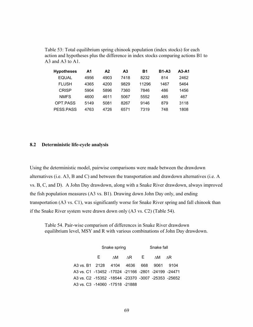
69
Table 53: Total equilibrium spring chinook population (index stocks) for eachaction and hypotheses plus the difference in index stocks comparing actions B1 toA3 and A3 to A1.
Hypotheses A1 A2 A3 B1 B1-A3 A3-A1EQUAL 4956 4903 7418 8232 814 2462FLUSH 4365 4200 9829 11296 1467 5464CRISP 5904 5896 7360 7846 486 1456NMFS 4600 4611 5067 5552 485 467
OPT.PASS 5149 5081 8267 9146 879 3118PESS.PASS 4763 4726 6571 7319 748 1808
8.2 Deterministic life-cycle analysis
Using the deterministic model, pairwise comparisons were made between the drawdown
alternatives (i.e. A3, B and C) and between the transportation and drawdown alternatives (i.e. A
vs. B, C, and D). A John Day drawdown, along with a Snake River drawdown, always improved
the fish population measures (A3 vs. B1). Drawing down John Day only, and ending
transportation (A3 vs. C1), was significantly worse for Snake River spring and fall chinook than
if the Snake River system were drawn down only (A3 vs. C2) (Table 54).
Table 54. Pair-wise comparison of differences in Snake River drawdownequilibrium level, MSY and R with various combinations of John Day drawdown.
Snake spring Snake fall
E �M �R E �M �R
A3 vs. B1 2128 4104 4636 668 9061 9104A3 vs. C1 -13452 -17024 -21166 -2801 -24199 -24471A3 vs. C2 -15352 -18544 -23370 -3007 -25353 -25652A3 vs. C3 -14060 -17518 -21888

70
A comparison of the base action (A1) to a natural river drawdown of John Day produced mixed
results for stocks depending on the assumptions made and the stocks being considered (Table
55). High transportation efficiency assumptions produced negative numbers in the A1 vs. C1
comparisons. That is, compared to the current operating conditions, equilibrium numbers and
MSY decreased with a John Day drawdown that also terminated the transportation program.
Using an assumption of low transportation effectiveness, C1 produced positive numbers for
Snake River spring and fall chinook relative to A1. For Hanford Reach fall chinook, John Day
drawdown was detrimental. Studies on the effectiveness of transporting Hanford Reach fish
from McNary dam suggest a high transport effectiveness for this system. Thus, transportation
was always better than passing the fish through the lower Columbia River hydrosystem. Upper
Columbia spring chinook, which are currently not transported from McNary dam, experienced a
small increased in equilibrium numbers and MSY with John Day drawdown.
Table 55: Difference in equilibrium population levels and MSY comparingbase action A1 to drawdown of John Day reservoir, C1.
EA1,C1 �MA1,C1 �RA1,C1
Snake River spring chinook -11791 to 2336 -2976 to 1280 2546 to -6346Snake River fall chinook -3428 to 6179 -1487 to 16791 18058 to -2793
Hanford Reach fall chinook -16876 -54066 -57322Upper Columbia spring chinook 184 91 165
8.3 Smolt passage analysis
Smolt passage information derived from the CRiSP passage model show small changes in travel
time for spring chinook and relatively large changes for fall chinook. For spring chinook, the
comparison was made only between full-pool travel time and the drawdown options. The
difference was two days between full pool and natural drawdown of John Day reservoir. Flood
control delayed fish an additional half-day. The spillway crest option gave results between full
pool and the natural river drawdown. There was little difference in the survivals between the
different C alternatives. Fall chinook exhibited a larger response to John Day drawdown with the

71
benefit of a decreased travel time up to one week. In a comparison between full pool and
drawdown of the Snake River dams plus the John Day Dam, the average in-river survival
changed from 0.29 to 0.51. The travel time of the fall chinook changed from 24 days to 13 days
between the two configurations.
8.4 Summary
To develop an understanding of the relative benefits of John Day drawdown under the Bayesian
model analysis, we compared results of a Snake River drawdown (A3) to the Snake River plus
John Day drawdown to natural river level (B1). The results in Table 56 used passage
assumptions that optimized the smolt and adult passage survival (OPT.PASS and HIGH.EJUV in
Tables 13 through 20). The difference in the measures of A3 and B1 illustrates the individual
contribution of a natural river drawdown of John Day reservoir. The drawdown contributed
nothing to Snake River spring and fall chinook recovery and survival probabilities. Under current
conditions (A1), the Bayesian analysis suggested equilibrium populations of about 5000 adults
for both spring and fall chinook. The John Day drawdown increased the equilibrium population
by approximately 20% for spring chinook and 50% for fall chinook.
Table 56: Difference in Snake River salmon survival and recoveryprobabilities and the difference in equilibrium populations between A3and B1. Results are from the Bayesian model with weightings ofhypotheses favoring optimum passage conditions.
� 24-yr
Surv. Prob.
� 48-yr
Recov. Prob.
EA3,B1
spring chinook -0.0005 0.022 879fall chinook 0.0005 0.011 2326
To characterize the effect of a John Day drawdown on the Upper Columbia and the Snake River
stocks, the deterministic model was used in pairwise comparison of actions. For actions without
transportation, the effect of John Day can be characterized by comparing action A3 to B1, B2 and
B3. That is, to characterize the effects of the John Day drawdown on the equilibrium conditions,
the difference in including a John Day drawdown to the Snake River drawdown is compared to a

72
Snake River drawdown alone. The maximum improvement of adding the John Day drawdown
was between 1 and 17%, depending on species (Table 57).
Table 57. Effects of John Day drawdowns are illustrated with pair-wisecomparisons to Snake River drawdown equilibrium levels.Equilibrium population under current condition, A1, is Equ. Pop. Thetotal Snake River spring chinook population is estimated assuming 38stocks.
Stock Equ. Pop. EA3,B1 EA3,B2 EA3,B3
Snake River spring chinook 15942 2128 190 1520Snake River fall chinook 7259 647 572
Hanford Reach fall chinook 132499 7602 5162 Upper Columbia spring chinook 1061 184 101 143
The impact of the actions on the pairwise difference of MYS plus escapement is illustrated in
Table 57a. The spring and fall chinook estimates were generated with high and low D values,
which give the least and most benefit to action B1, B2 and B3.
Table 57a. Effect of John Day drawdowns are illustrated with pair-wisecomparisons to Snake River drawdown equilibrium levels. Recruitmentplus harvest at MSY population under current conditions, A1, is RA1.Difference in R is �R. The total Snake River spring chinook population isestimated assuming 38 stocks.
Stock RA1 D �RA3,B1 �RA3,B2 �RA3,B3
Snake River spring chinook 4006 0.350.80
46362432
418190
32681710
Snake River fall chinook 3288 0.051.00
11043942
9667825
Hanford Reach fall chinook 190404 1.00 20358 13502 Upper Columbia spring chinook 422 NA 165 88 126
The effect of John Day drawdown without transportation, compared to the current transportation
of fish in A1, presents mixture benefits and detriments depending on the value of transportation
effectiveness as characterized by the D factor (Table 58). The maximum and minimum effects
are illustrated by comparing A1 to C1, C2 and C3. For Snake River stocks, when D is low, John
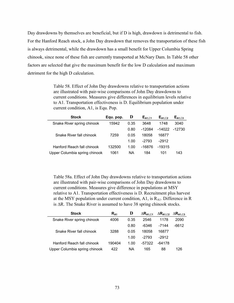
73
Day drawdowns by themselves are beneficial, but if D is high, drawdown is detrimental to fish.
For the Hanford Reach stock, a John Day drawdown that removes the transportation of these fish
is always detrimental, while the drawdown has a small benefit for Upper Columbia Spring
chinook, since none of these fish are currently transported at McNary Dam. In Table 58 other
factors are selected that give the maximum benefit for the low D calculation and maximum
detriment for the high D calculation.
Table 58. Effect of John Day drawdowns relative to transportation actionsare illustrated with pair-wise comparisons of John Day drawdowns tocurrent conditions. Measures give differences in equilibrium levels relativeto A1. Transportation effectiveness is D. Equilibrium population undercurrent condition, A1, is Equ. Pop.
Stock Equ. pop. D EA1,C1 EA1,C2 EA1,C3
Snake River spring chinook 15942 0.350.80
3648 -12084
1748-14022
3040-12730
Snake River fall chinook 7259 0.051.00
18058-2793
16877-2912
Hanford Reach fall chinook 132500 1.00 -16876 -19315 Upper Columbia spring chinook 1061 NA 184 101 143
Table 58a. Effect of John Day drawdowns relative to transportation actionsare illustrated with pair-wise comparisons of John Day drawdowns tocurrent conditions. Measures give difference in populations at MSYrelative to A1. Transportation effectiveness is D. Recruitment plus harvestat the MSY population under current condition, A1, is RA1. Difference in Ris �R. The Snake River is assumed to have 38 spring chinook stocks.
Stock RA1 D �RA1,C1 �RA1,C2 �RA1,C3
Snake River spring chinook 4006 0.350.80
2546-6346
1178-7144
2090-6612
Snake River fall chinook 3288 0.051.00
18058-2793
16877-2912
Hanford Reach fall chinook 190404 1.00 -57322 -64178 Upper Columbia spring chinook 422 NA 165 88 126
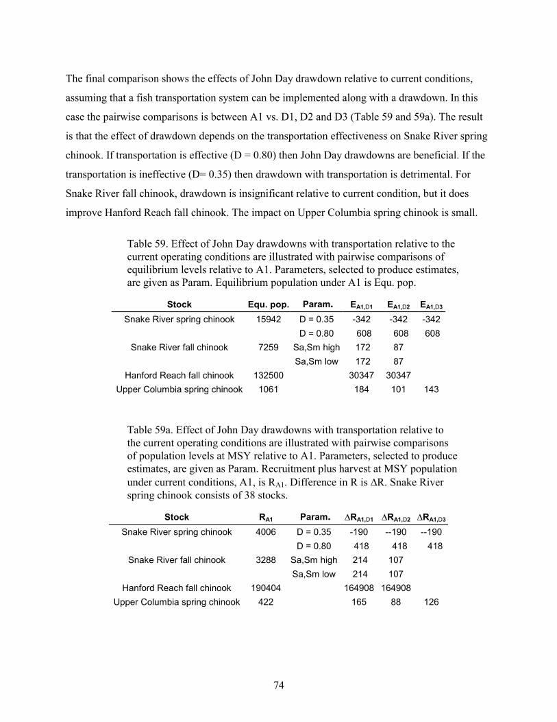
74
The final comparison shows the effects of John Day drawdown relative to current conditions,
assuming that a fish transportation system can be implemented along with a drawdown. In this
case the pairwise comparisons is between A1 vs. D1, D2 and D3 (Table 59 and 59a). The result
is that the effect of drawdown depends on the transportation effectiveness on Snake River spring
chinook. If transportation is effective (D = 0.80) then John Day drawdowns are beneficial. If the
transportation is ineffective (D= 0.35) then drawdown with transportation is detrimental. For
Snake River fall chinook, drawdown is insignificant relative to current condition, but it does
improve Hanford Reach fall chinook. The impact on Upper Columbia spring chinook is small.
Table 59. Effect of John Day drawdowns with transportation relative to thecurrent operating conditions are illustrated with pairwise comparisons ofequilibrium levels relative to A1. Parameters, selected to produce estimates,are given as Param. Equilibrium population under A1 is Equ. pop.
Stock Equ. pop. Param. EA1,D1 EA1,D2 EA1,D3
Snake River spring chinook 15942 D = 0.35D = 0.80
-342 608
-342 608
-342 608
Snake River fall chinook 7259 Sa,Sm highSa,Sm low
172 172
8787
Hanford Reach fall chinook 132500 30347 30347Upper Columbia spring chinook 1061 184 101 143
Table 59a. Effect of John Day drawdowns with transportation relative tothe current operating conditions are illustrated with pairwise comparisonsof population levels at MSY relative to A1. Parameters, selected to produceestimates, are given as Param. Recruitment plus harvest at MSY populationunder current conditions, A1, is RA1. Difference in R is �R. Snake Riverspring chinook consists of 38 stocks.
Stock RA1 Param. �RA1,D1 �RA1,D2 �RA1,D3
Snake River spring chinook 4006 D = 0.35D = 0.80
-190 418
--190 418
--190 418
Snake River fall chinook 3288 Sa,Sm highSa,Sm low
214 214
107107
Hanford Reach fall chinook 190404 164908 164908 Upper Columbia spring chinook 422 165 88 126

75
This analysis indicates that a John Day drawdown can have a positive or negative impact on the
stocks above the reservoir. The relative effects are clear when comparing the contribution of a
John Day reservoir drawdown to the drawdown of the Snake River dams. Under this comparison
the effectiveness of transportation is not a large issue, since neither action has transportation.
Then under the assumptions of the model, the contributions of John Day are incremental and
small. As illustrated in Table 57, spring chinook equilibrium increases by up to 2000 fish, while
the fall chinook increase by about 600 fish. The increase in the harvest plus escapement at MSY
(Table 57a) is up to four thousand spring chinook adults and eleven thousand fall chinook adults.
In comparison, the current equilibrium levels for the Snake River spring and fall chinook are
about sixteen thousand and seven thousand respectively. Historically, the runs were considerably
larger. In the 1950s, annual spring chinook returns to the Snake River were over one hundred
thousand adults and in the 1960s they were about sixty thousand. The Snake River fall chinook
spawning population, including escapement to the mouth of the Columbia and harvest, averaged
about seventeen thousand adults over the period 1966-1991 (Peters et al 1999). This level could
be obtained by fall chinook transportation, if the current transportation is ineffective (Table 58).
Furthermore, under this assumption, the contribution of improved passage with a John Day
drawdown is insignificant (Table 59). If fall chinook transportation is effective, then stopping
transportation decreases the population (Table 58).
8.5 Final Remarks
This analysis suggests that benefits of a John Day drawdown are uncertain. In general, the effect
of a John Day drawdown on Snake River fish depends on the assumptions about the extra
mortality and delayed mortality in transportation. If transportation is effective, then drawdown is
ineffective. If transportation is ineffective, then drawdown is effective. Hanford Reach fall
chinook are not improved with John Day drawdown, unless transportation is continued with the
drawdown. The Upper Columbia stocks generally are not affected by drawdown since the fish are
currently not transported and the change in survival with and without drawdown is small. In all
cases, a natural river drawdown is better than a spillway crest drawdown and flood control has an
insignificant impact on smolts passing through John Day reservoir.
76
9 References
Anderson, J.J., J. Hayes, P. Shaw, and R. Zabel. Columbia River Salmon Passage Model:
Theory, Calibration and Validation. Columbia Basin Research, Box 358218, University of
Washington, Seattle, 98195.
Anderson, J.J. 1999. Columbia River Salmon Passage Model: User Manual CRiSP 1.6.
Columbia Basin Research, Box 358218, University of Washington, Seattle, 98195.
Chapman, D., A. Giorgi, M. Hill, A. Maule, S. McCutcheon, D. Park, W. Platt, J. Seeb, L. Seeb,
and F. Utter. 1991. Status of the Snake River Chinook Salmon. Prepared for the Pacific Utilities
Conference Committee, February 19 1991 by Don Chapman Consultants, Inc., 3180 365
Rickenbacker, St 20. Boise, Idaho 83705.
Marmorek ed. 1996. Final report on the retrospective analysis for fiscal year 1996. Complied and
edited by ESSA Technologies Ltd. Vancouver, B.C.
Hinrichsen, R. A. and C. Paulsen 1998. Testing the hydro-related extra mortality hypothesis.
Submission 3 in PATH Weight of evidence Report. Complied and edited by ESSA Technologies
Ltd. Vancouver, B.C.
Marmorek and Peters ed. 1998. PATH weight of evidence report. Prepared by ESSA
Technologies Ltd. Vancouver, B.C.
Marmorek, D.R., C.N. Peters, and I. Parnell. (eds.) 1998. PATH Final Report for Fiscal Year
1998. ESSA Technologies, 1765 W. 8th Avenue, Suite 300, Vancouver, BC, V6J 5C6.

77
Peters, C.N., D.R. Marmorek, and I. Parnell. PATH Decision Analysis Report for Snake River
Fall chinook. ESSA Technologies, 1765 W. 8th Avenue, Suite 300, Vancouver, BC, V6J 5C6.
Ricker, W.E. 1978. Computation and Interpretation of Biological statistics of Fish Populations.
Bulletin 191, Department of the Environment Fisheries and Marine Science, Ottawa.
Schaller, H. A., C. E. Petrosky, and O. P. Langness. 1999. Contrasting patterns of productivity
and survival rates for stream-type chinook salmon (Onchorhynchuys tshawytscha) populations of
the Snake and Columbia rivers. Can J. Fish Aquat. Sci. 56: 1031-1045.
Smith, J.R. and S. Achord, 1999. Internal PATH document.
Zabel, R.W., and J.J. Anderson. 1997. A model of the travel time of migrating juvenile salmon,
with an application to Snake River spring chinook salmon. N. Amer. J. Fish. Manage. 17: 93-
100.
Zabel, R.W., J.J. Anderson, and P.A. Shaw. 1998. A multiple reach model describing the
migratory behavior of Snake River yearling chinook salmon (Oncorhynchus tshawytscha). Can.
J. Fish. Aquat. Sci. 55: 658-667.

78
10 Comments by PATH and Responses
10.1 Comments provided by Paul Wilson of CBWFW are included below.
Below are comments on the Sept. 13, 1999 draft of the paper. Many of these comments were made to two of theauthors on a conference call on Sept. 14. (Note: the numbering does not refer to this draft of the document)
Pg. 17, Table 3. Lower bound (pessimistic) estimates of survival rate through the free-flowing John Day reach wereused in PATH modeling, for both spring and fall chinook. The pessimistic estimate for spring chinook was a fixedvalue of 0.90 [EJUV1 – Marmorek et al. (1998), Table 2.2.1-1]. Note also that the optimistic survival rate valuewas 0.98, not .95, as indicated in Table 3. For fall chinook, modeled estimates of free-flowing survival rate, notfixed values, were used for both the optimistic and pessimistic values. The alternative assumptions differed inwhether there would be a decrease in fish travel time through the reach due to drawdown (Peters et al. 1999, Section5.2.2).
Pg. 20, Section 4.3. The term �o is not one that was used or defined within PATH. It appears the definitionintended here is “the base ocean survival common to transported and non-transported groups.” It’s not clear whatthe criteria are for including a PATH-modeled factor influencing post-Bonneville survival in �o as opposed to �n or�t. If �o is “contained within the exp(a) of the equation (sic) stock recruitment equation R = S exp(a – bS)”then the year effect (�y) of the Delta model in PATH is not contained in �o, and must somehow be applied to both�n and �t to be analogous to what was done in PATH
Pg. 22, Section 4.3.1. The three hypotheses about the trend in ocean mortality are not presented in an equitablemanner. The claim is made that, only for the hydro hypothesis, “a direct link between fish survival and hydrosystempassage has not been identified”, even though it’s the only hypothesis of the three for which a credible, directevidential link has been identified (see Schaller et al. 1999).
Pg. 23, Table 5. Description of �n as “characteristic ocean survival factor” is misleading, since it is really only thecomplement of the extra mortality experienced by Snake R. spring chinook. Ocean survival in the Delta model iscomposed of several modeled factors, including the year effect. By presenting �n as the ocean survival factor, itleads the reader to believe with FLUSH there is no apparent decline in ocean survival in the period from 1975 on.Inclusion of the year effect with FLUSH model estimates results in reduced ocean survival of spring chinook in theperiod 1975-90 compared to 1952-90.
Pg. 26, Table 8. Something seems to be amiss here: the conversion rates for B1 and B3 for spring chinook are lowerthan the A3 value. This makes no sense, unless a detriment to adult passage from dam removal is being assumed.
Pg. 41, Section 6. The text above eq. 17 indicates that hydrosystem passage corridor actions are never expected toalter the spawning habitat. However, in PATH an assumed increase in spawning habitat under Snake Riverdrawdown was simulated for fall chinook, when escapements were very high (Peters et al. 1999).
Pg. 42, Eq 18. Not necessary to estimate Smsy numerically. Hilborn (1985) presents direct formulas approximatingthe spawning level at MSY and MSY for the Ricker curve, and the conditions under which they are useable.
Pg. 46, Eq. 25. This formulation of the benefit of John Day drawdown plus Snake R. drawdown vs. Snake R.drawdown alone illustrates one of the limitations of this analysis. This equation assumes that there are benefits of B1

79
over and above A3 only in the juvenile and adult hydrosystem passage stages. In PATH, under the hydro extramortality hypothesis, there would be a benefit to post-Bonneville survival of actions that improve in-river conditionsfor smolts, such as John Day drawdown. We didn’t explicitly consider or model the additional benefits of SnakeRiver plus John Day drawdown compared to Snake River drawdown alone. Effectively, this analysis give a 100%weight to the hypothesis that there is no additional benefit to later life stages of a John Day drawdown, above that ofa Snake R. drawdown alone, and 0% to any other hypothesis. However, PIT tag studies indicate that post-hydrosystem survival of spring chinook smolts is influenced by hydrosystem passage experience (Sandford andSmith 1999, Schaller et al. 1999).
Pg. 48, Section 6.3.1. The number of spring chinook stocks in the Snake R. basin is indicated to be 24. This may beclose to the truth, but the ESU consists of both spring and summer chinook stocks, which number 35-40 total. Thus,the increase in the “Snake River Basin index spawning population” is underestimated by an amount proportional tothe underestimate in number of stocks in the ESU.
Pg. 52, first paragraph. The claim that “a drawdown of John Day reservoir without drawing down the Snake Riverreservoirs is not expected to increase ocean survival” is not a conclusion reached, or even discussed, in PATH. Wedid not do any analysis of scenarios where only John Day is drawn down. PIT tag data indicate that the higher thenumber of times a smolt passes a dam through bypass, the lower the SAR (Sandford and Smith 1999, Schaller et al.1999), suggesting that ocean survival decreases with number of dams passed.
Pg. 52, last paragraph. Upper Columbia spring chinook “G” is estimated with eq 25, which includes no effect oftransportation. Since, under A2, upper Columbia origin smolts would be transported at McNary dam, eq. 26 or 27 ismore appropriate. Tables 41 and 42 treat A1, A2, and A3 as identical in their effect on upper Columbia fish.Because of the MCN transport under A2, they are not. Also, A3 flow timing and magnitude in the lower Columbiawould be different from A1 and A2.
Pg. 60, Section 7.2.3. In tables 44 – 47, why weren’t B1 vs. A3 comparisons done? C1, C2 and C3 are notnecessarily good surrogates for gauging the effect of B1 or B2 vs. A3. Snake River drawdown would increase thewater velocity in the Snake, accelerating the arrival time of smolts to McNary dam in either CRiSP or FLUSH. Thiswould, for example, affect flows and temperatures, increasing flows and lowering temperatures experienced bysmolts in the lower part of the hydrosystem, and hence affect survival in John Day and the lower reservoirs.Differences of C1, C2, or C3 from. A1 are therefore likely underestimates of the additional benefits to smolt survivalprovided by John Day drawdown with Snake River drawdown.
Pg. 71, Section 8.5, last paragraph. Earlier comments detail why this analysis does not represent “the expected rangeof positive and negative impacts of a John Day drawdown.” The text about the Ricker equation here makes no sensein the context of this analysis. If Ricker equation is inappropriate, the biggest effect here would be to underestimatethe number of spawners resulting from B1, relative to A3 or any other scenario. This is because of the descendingright hand limb inherent in the Ricker curve. If productivity doesn’t decline at higher abundances, but stays aboutthe same, many more recruits per spawner would be produced at the higher abundances expected under A3 and B1scenarios.
References
Hilborn, R. 1985. Simplified calculation of optimum spawning stock size from Ricker’s stock recruitment curve.Can. J. Fish Aquat. Sci. 42: 1833-1834
Marmorek, D.R., C.N. Peters, and I. Parnell (eds.) 1998. PATH final report for fiscal year 1998. December 3,1998.
Peters, C.N., D.R. Marmorek, and I . Parnell (eds.). 1999. PATH decision analysis report for Snake River fallchinook (Draft 5). August 11, 1999.
80
Sandford, B. P. and S. G. Smith. 1999. Smolt-to-adult return percentages for Snake River basin salmonids, 1990-1995. NWFSC, Seattle.
Schaller, H., N. Bouwes, P. Budy, C. Petrosky, P. Wilson, O. Langness, E. Weber and E. Tinus. 1999. An analysisof differential delayed mortality experienced by stream-type chinook salmon of the Snake River. August 13, 1999Draft.
10.2 Response to review.
The responses to the review of P. Wilson and other PATH comments communicated by D.
Marmorek are listed below:
1. The differences in the Bayesian and deterministic methods was evaluated and resolved. The main result is the twoapproaches are mathematically equivalent and the differences in pairwise comparisons depend on inputs selected foreach method.
2. Concerns were considered related to the interpretation and characterization of ocean mortality using informationfrom the PATH analysis. The Bayesian analysis in this study was conducted with the programs used in PATH and sothe approach to characterizing ocean factors is identical to the PATH treatment. For the deterministic method, theapproaches are different. The deterministic approach looked at pairwise comparisons at equilibrium, allowing greatsimplification of the analysis. In this approach all factors that are common between two alternatives, whether they aretime variable or not, cancel. Because of this simplification basic differences in ocean survival need only reflect thedifferences resulting from the compared alternatives. Factors such as the ocean delta factor are subsumed into theRicker a parameter.
3. It was assumed in this analysis, as was done in PATH, that the John Day reservoir drawdown did not alter oceansurvival of stocks. The evidence for a linkage between ocean survival and passage experience remains uncertain andcontradictory. Studies suggesting ocean survival increases with passage through fewer bypass systems (Stanford andSmith 1999) are equivocal and more adult returns are needed to establish if a pattern exists. In PATH (Hinrichsenand Paulsen 1998) demonstrated there was no correlation between the post Bonneville survival and the juvenileinriver passage survival. In the analysis here, the effects of juvenile passage experience on ocean survival wereencompassed through the Hydro hypotheses for Snake River drawdown, but the possible effects of John Daydrawdown were not considered.
4. For spring chinook from the Snake River, the number of stocks in the September draft of this paper was 24. Thiswas changed to 32 spring and summer wild and natural stocks from the Snake River basin. This increased allestimates of stock numbers for equilibrium and the MSY levels by 1/3.
5. No attempt was made to evaluate the expansion of Ricker b factors by a drawdown action. The expansion of theSnake River fall habitat was not considered because the possible competition of Hanford Reach fall chinook for anynew habitat could not be resolved, in addition to this being beyond the scope of this study.
6. The MSY calculations were estimated exactly rather than through the Hilborn (1985) approximation. For thisstudy the Hilborn method was invalid.
References

81
Hinrichsen, R. and C. Paulsen. 1998. Testing the hydro-related extra mortality hypotheses. PATH document.
Hilborn, R. 1985. Simplified calculation of optimum spawning stock size from Ricker’s stock recruitment curve.Can. J. Fish Aquat. Sci. 42: 1833-1834
Sandford, B. P. and S. G. Smith. 1999. Smolt-to-adult return percentages for Snake River basin salmonids, 1990-1995. NWFSC, Seattle.