modeling the u.s. dairy sector with government...

Modeling the U.S. Dairy Sector withGovernment Intervention

Donald J. Liu, Harry M. Kaiser, Timothy D. Mount,and Olan D. Forker

An econometric framework for estimating a two-regime dairy structural system ispresented. Failure to account for switching between regimes due to government priceintervention raises the problem of selectivity bias. Further, since a structural system ofequations is involved, the problem is not limited to the market associated with theintervention. Rather, bias from a single source can distort all equations in the system.The ramifications of not correcting for the bias in policy analyses are investigated.

Key words: dairy, price intervention, switching simultaneous system, Tobit estimation.

The federal dairy price support program wasenacted in 1949 as a means of improving farmprices and incomes. Under this program, thegovernment attempts to support raw milk pric-es by buying an unlimited quantity of manu-factured dairy products at the wholesale levelwhenever the market price falls below the an-nounced government purchase price. The in-tervention of the government in this markethas broad-reaching effects not only on the farmlevel but also on the wholesale and retail levels.Our objectives are to: (a) investigate the im-plications of this type of intervention on theeconometric specification of a structural modelof the U.S. dairy industry and (b) examine theempirical ramifications of not using the ap-propriate specification in policy analyses.

When considering how prices in the dairysector are determined, the potential for gov-ernment intervention introduces a specialproblem. Prices are determined by differentforces depending upon whether the price es-tablished by competitive supply and demandconditions is above or below the governmentprice floor. If the competitively determinedmarket price for wholesale manufactured dairyproducts is above the government purchaseprice, a "market equilibrium" regime holds.

Donald J. Liu is an assistant professor in the Department of Eco-nomics at Iowa State University. Harry M. Kaiser is an associateprofessor, Timothy D. Mount and Olan D. Forker are professorsin the Department of Agricultural Economics at Cornell Univer-sity.

In this case, the observed wholesale manufac-tured price is the equilibrium price and hencegovernment intervention does not influence theprice formation process in the dairy sector. Onthe other hand, if the competitively deter-mined market price is below the purchase price,then a "government support" regime holds. Inthis case, the observed wholesale manufac-tured price equals the government price andthe government buys the excess supply at thatlevel. Hence, government intervention influ-ences the type of price formation process thatoperates in the market as well as the level ofprices.

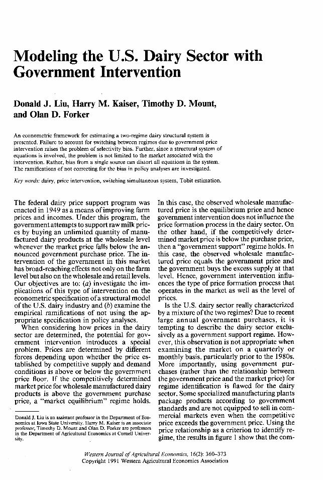
Is the U.S. dairy sector really characterizedby a mixture of the two regimes? Due to recentlarge annual government purchases, it istempting to describe the dairy sector exclu-sively as a government support regime. How-ever, this observation is not appropriate whenexamining the market on a quarterly ormonthly basis, particularly prior to the 1980s.More importantly, using government pur-chases (rather than the relationship betweenthe government price and the market price) forregime identification is flawed for the dairysector. Some specialized manufacturing plantspackage products according to governmentstandards and are not equipped to sell in com-mercial markets even when the competitiveprice exceeds the government price. Using theprice relationship as a criterion to identify re-gime, the results in figure 1 show that the com-

Western Journal of Agricultural Economics, 16(2): 360-373Copyright 1991 Western Agricultural Economics Association

Switching Dairy System 361

@3

0~a.0

00

0L.*0

C0

C0

c@3a

4Cc0C)IR'a000

C)4f

1975-1987 (QUARTERLY)

Relationship between the wholesale manufactured and government purchase price,

petitive regime held for 42% of the period1975-87. Even during the 1980s when dairysurpluses were relatively large, the competitiveregime occurred in 22% of that sample. Hence,with data from 1975 through 1987, it appearsthat the two-regime system should be consid-ered when specifying a model of the dairy sec-tor.

To date, econometric studies of the dairysector have not distinguished between the tworegimes and have instead assumed that thegovernment regime always occurs (Kaiser,Streeter, and Liu; LaFrance and de Gorter; Liuand Forker). This is due to the fact that thesestudies have not included a wholesale manu-factured dairy market where government in-tervention occurs. Failure to account forswitching between regimes raises the problemof selectivity bias, implying that conventionalleast squares estimates may be biased and in-consistent. Furthermore, since a structural sys-tem of equations is involved, these problemsare not limited to the market associated withthe intervention. Bias from a single source candistort all equations in the system. The issuehere is to determine whether these distortionsare important for policy analysis.

In the following sections, an econometricframework for estimating a two-regime dairystructural system is presented. Correcting forselectivity bias implies modifying the first stageof a conventional two-stage least squares es-

timator and providing an alternative set of in-struments for the second stage. Since the con-ventional two-stage least squares model is notnested in the bias-corrected model, Atkinson'stest for nonnested models is used to determinewhich one is supported best by the data. It isshown that the bias-corrected model is sup-ported in all equations, but the conventionalmodel is rejected in four out of five equations.Finally, the ramifications of using the conven-tional rather than the bias-corrected model inpolicy analyses are investigated by shockingpolicy variables in both models. The resultingimpacts on key endogenous variables are foundto be significantly different between the twomodels.

A Conceptual Framework

The econometric model of the dairy industryconsists of farm, wholesale, and retail levels.At the farm level, raw milk is produced andsold to wholesalers, who in turn process andsell it to retailers. Both wholesale and retaillevels are divided into a manufactured and afluid market. The construction is similar to aprevious model by Kaiser, Streeter, and Liuin that milk products are divided into fluidand manufactured dairy products. However,the previous model only considered the retailand the farm levels. The extension to include

Figure 1.1975-87

Liu et al.

Western Journal of Agricultural Economics

prfRETAILMANFSUPPLY

RETAIL MANFDEMAND

rm rm rmQ =Q Q

s d

pwf

Qw m Q wm

DFTAII

rf

Qwf QWf f

s dQu* g

Qfs

wm wfQ +Qs s

FARM MILK QUANTITY

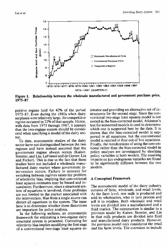
*To simplify, this figure ignores changes in commercial inventories, specialized plant quantity,and farm use.

Figure 2. Conceptual model of the U.S. dairy market

a wholesale level in this study facilitates theincorporation of government intervention inthe wholesale manufactured market. A sche-matic view of the various components of thedairy sector is presented in figure 2.

Government intervention occurs in thewholesale manufactured market for cheese,butter, and nonfat dry milk. Figure 2 illustratesthe occurrence of a government support re-gime, where the market equilibrium wholesale

manufactured price is below the governmentsupport price (Pg). In this case, Qdm is de-manded in the commercial market, which isless than what is supplied (Qwm), and the gov-ernment purchases the excess supply (Qg). Inthe case of the market equilibrium regime (notshown), the market equilibrium price is at orabove Pg, wholesale manufactured supplyequals demand, and Qg equals zero.

In the retail manufactured market, a general

pr m

pwm

pg

362 December 1991


specification for supply, demand, and the equi-librium condition can be written as:'

(la) In Qrm = a mln prm + frmln pwm

+ 7rmln Zrm + t ,rm

(lb) In Qrm = /3mln prm + _yrmln Zrm

+ irz, and

(lc) In Qm = In Qrm In Qrm,In QS d -

where Qrm and Qd are the retail manufacturedquantity supplied and demanded, Prm and pwmare the equilibrium retail manufactured priceand wholesale manufactured price, Zsr andZrm are vectors of exogenous supply and de-mand shifters pertaining to the retail manu-factured market, Qrm denotes the equilibriumretail manufactured quantity, and In is the nat-ural logarithm. The as, Os, and ys are the co-efficients, and ,t and Ad are error terms.

The retail fluid supply, demand, and equi-librium condition can be written following theform of the retail manufactured market as fol-lows:

(2a) In Qrf = af In prf + f In pwf

+ 7f ln Zf + Ar,

(2b) In Qu = Ofln prf + yf ln Zf

+ uf, and

(2c) In Q If = In Qf = In Qrf

where superscripts rfand wfrepresent the retailand wholesale fluid markets, respectively.

The wholesale manufactured supply, de-mand, and equilibrium condition (withoutgovernment purchases) are:

(3a) In Qwm = awmn pwm + _wmln P"

+ Y WMn Zwm + wm,

(3b) In Qm = In Qrm, and

(3c) In Qsm = ln(Qdm + QSP + AINV),

where pIi is the Class II price, QSP is the quan-tity of milk sold to the government by spe-cialized plants, AINVis change in commercialinventories of manufactured products, and all

' In the model that follows, we present a log-linear specificationbecause the empirical counterpart uses this specification. If a linearmodel is desired, simply replace the logarithm measurement byits level for all variables.

other variables are similarly defined with su-perscript wm denoting variables pertaining tothe wholesale manufactured market. Equation(3b) specifies that the wholesale manufactureddemand should equal the equilibrium retailmanufactured quantity as all the quantity vari-ables are expressed on a milk-equivalent basis.Finally, the variables QSP and AzINVare treat-ed as exogenous in this study because theycomprise a very small and rather constant por-tion of manufactured quantity.2

The wholesale fluid supply, demand, andequilibrium condition can be written followingthe form of the wholesale manufactured mar-ket as follows:

(4a) In Qwf = af Iln pwf + Iwfln(P"i + d)

+ yfln Zf + gf,

(4b)

(4c)

In Q"f = In QrS, and

In Qf = In QQf,

where d is the exogenous Class I differential.All other variables are defined as above withsuperscript wf denoting that the variables per-tain to the wholesale fluid subsector.

The wholesale manufactured price appear-ing in (la) and (3a) is constrained by the dairyprice support program. That is, since the gov-ernment sets a purchase price for storablemanufactured dairy products and is willing tobuy surplus quantities of the products at thatprice, the following constraint holds:

(5) In Pwm In Pg,

where Pg is the aggregate government purchaseprice for the manufactured products at thewholesale level.

When the government support regime holds,pwm simply equals Pg which is exogenous.However, the quantity of government pur-chases emerges as an additional endogenousvariable balancing the number of equationswith the number of unknowns. Accordingly,the equilibrium condition of (3c) for thewholesale manufactured market becomes:

(3c') In Qwm = ln(Qd'" + QSP + AINV + Qg),

where Qg is government purchases measuredon a milk-equivalent basis.

2 While small does not by itself guarantee exogeneity (Binkley),the first differences of these variables appear to be stationary witha strong seasonal pattern. Hence, they are treated as being exog-enous.

Liu et al.


Given the retail and the wholesale equationsin (1)-(5), the dairy model can be completedby introducing the farm market. To simplify,it is assumed that dairy farmers' price expec-tations are based solely on lagged prices. Ac-cordingly, the farm supply equation is speci-fied as:

(6a) In Qf =af In L(Pf) + -yln L(Z) + Afwhere Q is the farm milk supply, Pis the farmmilk price, thefsuperscript represents the farmmarket, and L is the lag operator with L(X) -X_,. Since milk used for fluid and manufac-tured purposes commands different prices, thefarm milk price is related to the average of theClass I and Class II prices via the followingequation:

(6b) p - (p" + d)*Qwf + II* Qwm(6b) Pf = v ;

(Qf - FUSE)

where FUSE is on-farm use of milk, which isassumed to be exogenous. Finally, the farm-level equilibrium condition is:

(6c) In Qf{ = ln(Qwf + Qwm + FUSE).

To summarize, because of the naive farmprice expectation assumption, the farm milksupply is predetermined at each point in time.3Hence, the above dairy model is recursive innature consisting of a retail-wholesale subsys-tem [equations (1)-(5)] and a farm market[equations (6a-c)]. The focus of this study isto examine the appropriate estimation pro-cedure for the retail-wholesale subsystem, giv-en the recursive structure of the dairy model. 4

The retail-wholesale subsystem encompassestwo possible regimes. In the case of the market

3Previous studies in farm milk supply have found that usinglagged prices as proxies for price expectations fits the data well(e.g., Chavas and Klemme; Kaiser, Streeter, and Liu; and Liu andForker). On the other hand, LaFrance and de Gorter employedthe current price of milk in the supply equation and used instru-mental variable methods to deal with simultaneous determinationof supply and demand. To assess the appropriateness of the pre-determined farm milk supply in our quarterly model, the Hausmanendogeneity test was conducted. The hypothesis that the farm milksupply was not predetermined was rejected at the 5% significancelevel. Specifically, if Qf is predetermined, the reduced form for thefarm milk price in (6b) can be estimated as a function of all ex-ogenous variables in the system, including QA. On the other hand,if Qf is not predetermined, it has to be replaced by an appropriateinstrument [say, L(Q2)] in the above regression. If the assumptionthat Qf is predetermined is correct, then the difference in the co-efficients from the two reduced-form estimations should be closeto zero.

4 The farm market equation was estimated in Liu et al. (1990)and the whole dairy model was used to conduct policy simulationsinvolving various generic dairy advertising scenarios.

equilibrium regime, the endogenous variablesare: retail manufactured demand and supplyand wholesale manufactured demand (Q m =Qrm = Qdm), wholesale manufactured supply(Qwm), retail and wholesale fluid supply anddemand (Qf = Qu = Qwf = Qf), retail manu-factured price (Prm), wholesale manufacturedprice (Pwm), retail fluid price (PR), wholesalefluid price (Pwe), and Class II price (PI). Theexogenous variables, denoted by Z, are:

Z = (Zr , Zrm , Zrf Z , Zs, Zwf Q, d,FUSE, QSP, AINV).

In the case of the government support regime,Qg replaces Pwm as an endogenous variable inthis list, and the exogenous variables, denotedby Z,, are

Z, = (Z, Pg).

The Switching System Estimation Procedure

Taking the unconditional expectation of thestructural equations (la), (lb), (2a), (2b), (3a),and (4a) yields:

(7a) E[ln Qrm] = armE [ln prm]

+ frmE[ln pwm] + 7ymln Zr,

(7b) E[ln Qrdn] = Pf3mE[ln prm] + y mln Zm,

(7c) E[ln Qf] = arE[ln Prf]

+ rlE[ln Pwf] + y7f n Z+ ,

(7d) E[ln Qr] = /53E[ln prf] + %yln Zf,

(7e) E[ln Qwm] = awmE[ln pwm] + /3WmE[ln P"]

+ ywmln Z m , and

(7f) E[ln Qwf] = asYfE[lnPwf] + j1wfE[ln(PIn + d)]

+ ?yfln Zsf.

The estimation procedure is analogous toconventional two-stage least squares, consist-ing of the following two steps. The first step isto estimate the expected prices in the right-hand side of (7a)-(7f) to be used as instru-mental variables for prices in the structuralequations estimation of the second step. Oncethe instrumental variables for price (hereafterreferred to as price instruments) are obtained,the second step involves a straightforward ap-plication of ordinary least squares to the struc-tural equations (la), (lb), (2a), (2b), (3a), and(4a) with the price instruments replacing the

364 December 1991


observed prices. The task is to obtain a con-sistent estimate of the reduced-form price in-struments.

Since the underlying market structures aredifferent between regimes, there are two setsof reduced-form equations with different en-dogenous variables (Pwm or Qg) and differentsets of exogenous variables (Z or Z*). In themarket equilibrium regime, the reduced-formequations for the prices are:

(8a) In pwm = Irwmln Z + ewm > In Pg and

(8b') In pi = rni In Z* + E* i = rm, rf wf II,

In the government support regime, the re-duced-form equations are:(8a') In pwm = In pg and

(8b') In Pi = rn In Z* + e* i = rm, rf wf, II,

where equations (8b) and (8b') pertain to retailmanufactured price, retail fluid price, whole-sale fluid price, and Class II price. It is im-portant to note that the structural error terms,AUs, enter the log-linear price reduced-formequations in an additive fashion. Hence, theprice reduced-form error terms will be nor-mally distributed if the structural error termsare normally distributed. Since normality of esis important to the procedure that follows, wedemonstrate the connection using a simple two-market model in the appendix.

Define the probability that the governmentsupport solution occurs as · and the proba-bility that the market equilibrium solution oc-curs as 1 - (. That is,

PROB{ln pwm C In Pg} and1 - - PROB{ln pwm > In Pg}.

Consider first the reduced-form equation forthe wholesale manufactured price in (8a) and(8a'). Since this price is constrained to not beless than the government purchase price, theuse of ordinary least squares to estimate (8a)results in selectivity bias. Combining the tworeduced-form equations in (8a) and (8a') forthe two solution regimes weighted by their re-spective probabilities and taking the uncon-ditional expectation of the resulting expressionyields:

(9) E[ln Pwm] = (1 - ))E[ln wm I lnPwm > In Pg]+ · In Pg.

Assuming that Ewm is normally distributed,E[ln pwm In Pwm > In Pg] can be expressed as(Maddala, pp. 158-59):

(10) E[ln Pwm lnPwm > In Pg]= rwmln Z + a{((c)/[l - b(c)]},

where 4(c) and ¢(c) are, respectively, the cu-mulative standard normal and the standardnormal density, both evaluated at c which isdefined as (In Pg - Trwmln Z)/a, and a2 is Var[ewm].The coefficients for T.

wm and a, as well as for 4and , in (10), can be estimated simultaneouslyand consistently by applying a maximum like-lihood Tobit procedure on (8a). The last termin (10) is the Heckman correction term forselectivity bias (Heckman). Then, by substi-tuting (10) into (9), the price instrument forthe wholesale manufactured price is:

(11) E[ln Pwm] = (1 - )Trwmln Z + fln Pg+ oa.

Now consider the reduced-form equationsfor the unconstrained prices (i.e., retain man-ufactured price, retail fluid price, wholesalefluid price, and Class II price) in (8b) and (8b').Combining the two reduced-form equationsfor the two solution regimes weighted by theirrespective probabilities and taking the uncon-ditional expectation of the resulting expressionyields:

(12) E[ln P] -(1 - )({r'lnZ+ E[ei IlnPwm > ln Pg]}

+ · {irrln Z,+ E[E i nPwm < InP g]}.

Assuming the joint density of Emw and ei is bi-variate normal and making use of (8a), thefollowing holds: 5

(13)E[€i I In p"m > In Pg] = E[ei Ewm > In Pg - Twmln Z]

= ((a/a){¢(C)/[ - (C)]},

where a' is COV[Ewmi].Similarly, assuming the joint density of Ewm

and e* is bivariate normal and making use of(8a), the following holds:

5 Assuming that the joint density ofx and y is bivariate normalwith zero means, Johnson and Kotz show that

E[x I y > z] = {COV[x, y]/SD[y]}-{p(4)/(l - ¢(0))}, andE[x I y < z] = -{COV[x, y]/SD[y]}{/(4)/A(4)},

where COV and SD are the covariance and standard deviationoperators and 4 is defined as z/SD[y].

Liu et al.

Western Journal ofAgricultural Economics

(14)E[Ei | In Pwm < In Pg] = E[e. ewm < In g -_rwmln Z]

= - ('i./)){0(c)/A(c)},

where art is COV[ewmEl]. The price instrumentfor the unconstrained prices may be obtainedby substituting (13) and (14) into (12) to give:

(15)E[ln P] = 7ri[(1 - )ln Z] + 7ri [ In Zj]

+ (a' - T')[0/a].

With estimates of ~, ¢, and (o from the Tobitestimation in (10), the parameters 7ri, -rx, and(aI - ai) in (15) can be estimated by ordinaryleast squares with the observed values of In Preplacing E[ln P']. The last term in (15) resem-bles the Heckman correction term in (10).

To summarize, rather than regressing eachendogenous variable on all exogenous vari-ables to obtain the price instrument, the re-duced-form equation for the wholesale man-ufactured price should be estimated by a Tobitprocedure while those for other endogenousprices should be fitted to a weighted averageof the exogenous variables from each regimewith a Heckman-like correction term append-ed.

prehensive model is obtained by augmentingthe government purchase price (In Pg) into theexogenous vector Z in the first term of (15):

(17) E[ln P] = 7ra[(1 - b)ln Z.] + 7r*[Q In Z.]

+ (i - -*)[0/4],

where the augmented parameter vector -rx con-tains iri and an additional parameter (i) forthe government purchase price.

The bias-corrected model in (15) can be ob-tained by imposing the following single restric-tion on the comprehensive model (17):

(18) {i= 0.

An F-test on (18) can be used to determine theappropriateness of the bias-corrected model.Similarly, an F-test on the following set of re-strictions can be used to determine the appro-priateness of the conventional model in (16):

a -_ a = 0.

The Estimation Results

7r - 7r = O and(19)

Tests Against the Conventional Model

To investigate whether the above bias-cor-rected procedure matters empirically, the fol-lowing tests can be applied to the reduced-formequations. With respect to the wholesale man-ufactured price reduced-form equation in (10),the second term on the right-hand side is theHeckman correction term for selectivity bias.Hence, a t-test for the estimate of a can be usedto determine the existence of the bias if ordi-nary least squares is used instead of the Tobitprocedure.

With respect to the remaining four uncon-strained price reduced-form equations in (15),a procedure based on the Atkinson nonnestedmodels test is used to compare models (At-kinson; Judge et al., p. 438). Specifically, thereare two nonnested models that need to be com-pared, the bias-corrected model represented by(15) and the conventional two-stage leastsquares reduced-form model which is:

(16) E[ln P] = 7rl1n Z..

Following Atkinson, a comprehensive modelcomposed of both (15) and (16) is constructedto test the two competing models. The com-

Based on the conceptual model, there are sixstructural equations that need to be estimated:retail fluid demand, retail manufactured de-mand, retail fluid supply, wholesale fluid sup-ply, retail manufactured supply, and wholesalemanufactured supply. These equations are es-timated simultaneously by the switching re-gime estimation procedure discussed previ-ously using quarterly data from 1975 through1987.6

6 The data used to estimate the structural equations come froma variety of sources. Selected years of Federal Milk Order MarketStatistics [U.S. Department of Agriculture (USDA) 1970-88a] wereused for the Class II price, Class I differential, and retail andwholesale fluid demand and supply. Selected issues of Dairy Sit-uation and Outlook (USDA 1970-88b) were used for milk pro-duction, net government price support program purchases, com-mercial inventories, and on-farm use of milk. This source also wasused to construct the retail manufactured price index, which is aweighted average of retail cheese, butter, and ice cream price in-dices. It also was used to construct the aggregate government pur-chase price and wholesale manufactured market price. The Hand-book of Basic Economic Statistics (Bureau of Economic Statistics)was used for the average hourly wage in manufacturing and civilianpopulation. U.S. Department of Labor (USDL), Bureau of LaborStatistics' publications Consumer Price Index (USDL 1970-88a),Producer Price Index (USDL 1970-88c), and Employment andEarnings (USDL 1970-88b) were used to obtain data on all retailand wholesale prices and on the unemployment rate and disposableincome. Finally, Leading National Advertisers (Leading NationalAdvertisers, Inc.) was used for generic advertising expendituresfor fluid and manufactured products. A detailed description andlisting of the data is presented in Liu et al. (1989).

366 December 1991


Table 1. Estimated Structural Equations (The Bias-Corrected Model)

ln(Qf/POP) = -2.236 - .282 ln(Pr/INC) + .154 ln(PBEV/INC) + .0025 In DGFA(-14.88) (-2.34) (2.31) (2.01)+ .004 In DGFA_, + .0045 In DGFA 2 + .004 In DGFA_3 + .0025 In DGFA_4

(2.01) (2.01) (2.01) (2.01)- .179 in TIME - .028 SINi + .083 COS1 +.517,4_,

(-6.79) (-3.60) (10.70) (3.24)Adj. R2 = .88 Durbin-Watson = 1.84

ln(Qrm/POP) = -2.467 - .928 In(Prm/INC) + .645 ln(PMEA/INC) + .0009 In DGMA(-10.42) (-2.68) (2.29) (1.64)+ .0014 In DGMA_, + .0016 In DGMA_2 + .0014 In DGMA_3 + .0009 In DGMA_4

(1.64) (1.64) (1.64) (1.64)- 1.436 lnDPAFH + .071 In TIME - .050 SIN1 - .085 COSi

(-2.09) (2.64) (-4.92) (-8.29)Adj. R2 = .85 Durbin-Watson = 2.07

In Qf = 2.809 + .940 ln(Pf/Pwf) - .111 ln(PFE/Pwf) - .015 UNEMP(6.00) (1.82) (-3.68) (-3.95)+ .237 in Qf,- .227 In Qrf - .001 TIME - .052 SIN1 + .094 COS1

(1.76) (-1.98) (-1.90) (-3.90) (8.14)Adj. R2 = .90 Durbin-h = 1.60

In Qm = -1.507 + .683 ln(Pm/Pw-) - .334 ln(MWAGE/P wm) - .042 COS1(-1.69) (2.37) (-1.51) (-2.78)+ .163 In Qrm + .581 In Qr4

(2.21) (6.55)Adj. R2

= .93 Durbin-h = 1.36

In Qwf= 2.184 + .381 ln(Pwf/(PII + d)) - .093 ln(PFE/(P" + d)) - .016 UNEMP(4.03) (2.66) (-2.85) (-3.98)+ .240 In Qf, - .223 In Qwf4 - .003 TIME- .050 SIN1

(1.79) (-1.96) (-3.74) (-3.74)+ .094 COS1

(8.18)Adj. R2 = .90 Durbin-h = 1.13

In Q m = .528 + .870 In(Pwm/P) - .544 ln(MWAGE/P") - .122 POLICY(2.70) (1.50) (-2.86) (-4.37)+ .301 In Qwm + .351 In Qwm + .00017 TIME 2 + .077 SIN1

(3.40) (4.15) (4.29) (4.08)- .125 COS1 + .751 , wm

(-6.42) (4.05)Adj. R2

= .96 Durbin-h = .25

The retail fluid and manufactured demandequations are estimated on a per capita basis,while the retail and wholesale supply equationsare estimated on a total quantity basis becausepopulation is not a supply determinant. Bothdemand equations are expressed as functionsof their own price, per capita income, price ofsubstitutes, advertising, a time trend, harmon-ic seasonal variables, and other shifters. Thesupply equations are expressed as functions oftheir own price, input prices, lagged supply,harmonic seasonal variables, and other shift-ers. The estimation results are in table 1. All

the estimated coefficients have correct signsand are significant at conventional confidencelevels (as indicated by the t-values in paren-theses). The adjusted R-squared, Durbin-Wat-son statistics, and Durbin-h statistics suggestgood fit of the data. A more specific explana-tion of the equations follows.

Per capita retail fluid demand (Qc/POP) isestimated as a function of the ratio of the retailfluid milk price index (P) to per capita income(INC), the ratio of the retail nonalcoholic bev-erage price index (PBE V) to per capita income,deflated generic fluid advertising expenditures

RetailFluidDemand

RetailManufac-

turedDemand

RetailFluidSupply

RetailManufac-

turedSupply

WholesaleFluidSupply

WholesaleManufac-

turedSupply

Liu et al.


(DGFA), a time trend (TIME), and two har-monic seasonal variables (SINl and COS1).7The specification of the two price-to-incomeratios is consistent with the zero homogeneityassumption for prices and income (Phlips, pp.37-38). The beverage price index is a proxyfor the price of fluid product substitutes. Thecurrent and lagged advertising variables ac-count for the impact of advertising on de-mand.8 The time trend (first quarter of 1975equals one) captures the effect of changes inconsumer preferences over time, specifically,the increasing concern about the link betweenheart disease and fluid milk consumption. Thetwo harmonic seasonal variables capture sea-sonality in demand. Based on the estimatedautocorrelation function and partial autocor-relation function of the residuals, a first-ordermoving-average error structure is imposed. Allthe coefficients remain stable after imposingthe moving-average term.

Per capita retail manufactured demand(Qrm/POP) is estimated as a function of theratio of the retail manufactured price index(Pm) to per capita income, the ratio of the retailmeat price index (PMEA) to per capita in-come, deflated generic manufactured advertis-ing expenditures (DGMA), the deflated retailprice index for food away from home (DPAFH),a time trend, and the two harmonic seasonalvariables. The meat price index is a proxy forthe price of manufactured product substitutes.The away-from-home price index is includedbecause a large portion of cheese is consumedaway from home. The trend variable measuresthe increase in consumer preferences for cheeseand yogurt. Unlike fluid products, consumersdo not perceive manufactured products suchas cheese as high-fat products even though theycontain as much fat as whole milk (Cook etal., p. 9).

Retail fluid supply (Qr) is estimated as afunction of the ratio of the retail fluid priceindex to the wholesale fluid price index (Pw),

7 All deflated price variables are defined as the nominal measuredivided by the Consumer Price Index for all items (1967 = 100).The variables COS1 and SIN1 represent the first wave of the cosineand sine, respectively (Doran and Quilkey). The variable POP isthe population of the United States.

8 The impact of current and lagged fluid advertising expenditureson demand is specified as a second-order polynomial distributedlag with both end point restrictions imposed. The appropriatenessof the end point restrictions was tested and not rejected. Thisspecification is consistent with Ward and Dixon. The same spec-ification is used for the manufactured advertising expenditures inthe retail manufactured demand equation.

the ratio of the fuels and energy price index(PFE) to the wholesale fluid price index, laggedsupply, the unemployment rate (UNEMP), atime trend, and the harmonic seasonal vari-ables. The specification of the retail-to-whole-sale price ratio and the energy price to thewholesale price ratio is consistent with the zerohomogeneity assumption for prices. Thewholesale fluid and energy prices represent twoof the most important costs in fluid retailing.The two lagged dependent variables are in-cluded to capture short- and longer-term pro-duction capacity constraints. 9 The unemploy-ment rate is used as a proxy for the state ofthe economy. The time trend is included tocapture other determinants of supply such aslabor costs in the retail fluid sector, which areunavailable.

Retail manufactured supply (Q rm) is esti-mated as a function of the ratio of the retailmanufactured price index to the wholesalemanufactured price index (Pwm), the ratio ofthe average hourly wage rate in the manufac-tured sector (MWAGE) to the wholesale man-ufactured price index, lagged supply, and a har-monic seasonal variable. The wholesalemanufactured price accounts for the largestportion of variable costs, and the manufac-tured wage rate measures labor costs in man-ufactured retailing. The energy price and un-employment rate were included in the initialestimation of this equation, but were subse-quently omitted due to their coefficients beingof the wrong sign. Also, the trend variable andSIN1 were omitted due to insignificant coef-ficients. The exclusion of TIME and SIN1 didnot change the results of the estimation sig-nificantly.

Wholesale fluid supply (Qwt ) is estimated asa function of the ratio of the wholesale fluidprice index to the Class I price for raw milk(pi = pn + d), the ratio of the fuels and energyprice index to the Class I price, lagged supply,the unemployment rate, a time trend, and theharmonic seasonal variables. The Class I priceis included because it represents the most im-portant cost in fluid wholesaling.

Wholesale manufactured supply (Qwm) is es-timated as a function of the ratio of the whole-sale manufacturing price index to the Class II

9 The eigenvalues for this dynamic system have real parts all lessthan one in absolute value indicating the equation is stable. Thestability condition also is satisfied for other dynamic supply equa-tions presented here.

368 December 1991


Table 2. F-Tests for the Price Reduced-Form Equations

Bias-Corrected Model Conventional ModelEquation F(1,6) P-Valuea F(22,6) P-Value

Retail Fluid Price (PI) .22 .66 1.54 .31Retail Manufactured Price (prm) .61 .47 4.21 .04

(Rejected)Wholesale Fluid Price (Pwl 3.09 .13 4.87 .03

(Rejected)Wholesale Manufactured Price (Pwm) (Rejected)bClass II Price (P") .83 .40 5.52 .02

(Rejected)a At (1 - a)% confidence level, one rejects the model if the P-value is less than a.b Based on the t-ratio on the Heckman-like correction term in equation (9).

price (P"), the ratio of the manufactured wageto the Class II price, lagged supply, a policydummy variable (POLICY), a time trend, andthe harmonic seasonal variables. The Class IIprice is included because it represents the mostimportant variable cost in manufacturedwholesaling. The policy dummy variable (equalto one for the first quarter of 1984 through thesecond quarter of 1985 and the second quarterof 1986 through the third quarter of 1987) ac-counts for the significant reductions in raw milksupply due to the implementation of the MilkDiversion Program and the Dairy Termina-tion Program, which had large impacts on thewholesale manufactured market. A first-ordermoving-average error structure is imposed tocorrect for serial correlation in the residuals.All the coefficients remain stable after impos-ing the moving-average term.

Tests for Selectivity Bias in theConventional Model

As previously indicated, a significant t-statisticfor the coefficient (a) on the Heckman correc-tion term in (10) signifies the existence of se-lectivity bias in the wholesale manufacturedprice reduced-form equation if ordinary leastsquares (instead of Tobit) is used. The t-sta-tistic for the estimated a is 6.4 using a maxi-mum likelihood Tobit estimation procedure. 10

This supports the statistical relevancy of theTobit procedure for the constrained wholesalemanufactured price reduced-form equation.

The tests for the remaining four reduced-form equations of the unconstrained prices (re-

10 The t-ratio for the estimate of a using a Heckman two-stepestimation procedure (Maddala, pp. 158-59) is 5.24.

tail fluid price, retail manufactured price,wholesale fluid price, and Class II price) arebased on the Atkinson procedure discussed in(15) to (19). The P-values for the F-statisticsare presented in table 2. At the 95% confidencelevel, the bias-corrected model cannot be re-jected for all four equations. On the other hand,the conventional model is rejected for all ofthe price reduced forms except the retail fluidprice. The result that the conventional modelcannot be rejected for the retail fluid price isnot that surprising because this market prob-ably has the weakest linkage to the supportedwholesale manufactured market.

The above tests provide statistical evidencethat selectivity bias is not simply a problemfor the price directly influenced by governmentintervention. It also affects other price re-duced-form equations in the system.

Empirical Implications for Policy Analysis

While we have shown that the conventionalmodel suffers from selectivity bias, it is usefulto examine the differences in the magnitudesof estimated structural parameters between thetwo models. It is also useful to investigatewhether the two models generate different pol-icy conclusions. To provide the basis for thesecomparisons, the conventional model is esti-mated using two-stage least squares assumingthe government purchase price is always bind-ing. The estimation results are presented intable 3.

The estimated structural equations are sim-ilar to those of the bias-corrected model withrespect to goodness of fit, t-values, Durbin-Watson and Durbin-h statistics. The major dif-

Liu et al.


Table 3. Estimated Structural Equations (The Conventional Model)

ln(Qf/POP) = -2.253 - .267 ln(Prf/INC) + .149 ln(PBEV/INC) + .0025 In DGFA(-14.61) (-2.13) (2.17) (1.96)+ .004 In DGFA_, + .0045 In DGFA_2 + .004 In DGFA_3 + .0025 In DGFA_4

(1.96) (1.96) (1.96) (1.96)- .176 In TIME - .028 SIN1 + .082 COS1 + .502 y_,

(-6.46) (-3.54) (10.51) (3.15)

Adj. R2 = .87 Durbin-Watson = 1.85

ln(Qdm/POP) = -2.601 - .655 In(Prm/INC) + .432 In(PMEA/INC) + .0008 In DGMA

(-10.97) (-1.85) (1.55) (1.30)+ .0013 In DGMA, + .0014 In DGMA_2 + .0013 In DGMA_3 + .0008 In DGMA_4

(1.30) (1.30) (1.30) (1.30)- 1.061 lnDPAFH + .082 In TIME - .050 SIN1 - .085 COS1

(-1.48) (2.82) (-4.71) (-7.98)

Adj. R2 = .84 Durbin-Watson = 2.08

In Qrf= 2.856 + 1.108 ln(Pf/Pwf) - .111 In(PFE/Pwf) - .016 UNEMP

(6.17) (1.98) (-3.74) (-4.06)+ .230 In Qrl - .245 In Qr( - .001 TIME - .052 SIN1 + .096 COS1

(1.73) (-2.13) (- 1.74) (-3.94) (8.23)

Adj. R2 = .90 Durbin-h = 1.75

In Qr = -2.197 + .897 ln(pm/Pwm) - .506 ln(MWAGE/Pwm ) - .045 COS1

(-2.09) (2.64) (-1.96) (-2.95)+ .167 In Qr" + .560 In Qrm"

(2.30) (6.20)Adj. R

2 = .93 Durbin-h = 1.36

In Qf = 1.950 + .461 ln(Pwf/(P" + d)) - .085 ln(PFE/(P" + d)) - .016 UNEMP

(3.30) (2.72) (-2.49) (-4.08)+ .221 In Qs, - .203 In Qwf - .003 TIME - .047 SIN1 + .093 COS1

(1.66) (-1.83) (-3.77) (-3.44) (8.33)

Adj. R2 = .90 Durbin-h = 1.13

In Q m = .285 + 1.117 ln(Pwm/P"I) - .431 In(MWAGE/P") - .113 POLICY

(1.41) (1.19) (-2.26) (-3.83)+ .422 In Qsw + .335 In Qwe + .00014 TIME 2 + .100 SIN1 - .123 COS1

(5.01) (3.76) (3.30) (4.74) (-6.14)+ .617 sw_

(3.54)Adj. R2 = .96 Durbin-h = .25

ference between the two models lies in themagnitudes of the price coefficients. In general,the conventional model has smaller own-pricecoefficients in the demand equations and largerprice coefficients in the supply equations. Forexample, the own-price coefficients in the re-tail manufactured supply equations are .897for the conventional model and .683 for thebias-corrected model. On the other hand, theown-price coefficients in the retail manufac-tured demand equations are -. 655 for the con-ventional model and -. 928 for the bias-cor-rected model.

To investigate whether the two models gen-erate different policy conclusions, dynamicimpulse analyses are conducted on the con-ventional and the bias-corrected models. Two

policy variables are of interest: the governmentpurchase price (Pg) and the Class I differential(d). The levels of these two variables are ofinterest because they have been the key policyinstruments set by Congress and the Admin-istration in the 1985 and the 1990 farm bills.It is assumed that the dairy sector is in a steadystate in which all the variables are set at athree-year average of 1985-87. The two mod-els are shocked with a permanent 10% increasein the government purchase price, and the im-pacts on the endogenous variables are simu-lated for 20 quarters. A similar analysis is con-ducted with a 10% shock in the Class Idifferential. The models are solved using theGauss-Seidel method.

In general, the endogenous variables con-

RetailFluidDemand

RetailManufac-

turedDemand

RetailFluidSupply

RetailManufac-

turedSupply

WholesaleFluidSupply

WholesaleManufac-

turedSupply

370 December 1991


PII ($/cwt.)1 R: r: n _

15.00

14.50

14.00

13.50

13.00

12.50

12.00

11.50

11.00

a -4-3-2-1 0 1 2 3 4 5 6 7 8 9 1011121314151617181920

Quarter

Figure 3a. Impact of 10% permanent shockin the government purchase price on the ClassII price

verge to a new steady state within two yearsregardless of which model is used. In addition,the pattern of the convergence from the twomodels is similar for most variables. However,the level of the time paths differs significantlyfor some variables, as illustrated in figures 3a-3d. In these figures, the preshock steady state(quarters -4 to -1) and the adjustment paths,resulting from the shock (at quarter 0), for theClass II price and government purchases arepresented. With a permanent 10% shock in thegovernment purchase price, the Class II pricein the conventional and bias-corrected modelsreaches a new steady state of $13.40 and$15.12, respectively, from an old steady stateof $11.33 (figure 3a). With a permanent 10%shock in the Class I differential, governmentpurchases decrease from an old steady state of2.54 billion pounds per quarter to 1.64 and1.40 billion pounds, respectively, which rep-resents an annual difference of about one bil-lion pounds between the two models (figure3b).

However, the differences between models are

2.55

2.50

2.45

2.40

2.35

2.30

2.25

3ias-Corrected

Conventionaln 1

2 .2 0 lI i i i l l l i i i i i l i i I i i iC -4-3-2-1 0 1 2 3 4 5 6 7 8 9 1011 121314151617181920

Quarter

Figure 3c. Impact of 10% permanent shockin the government purchase price on govern-ment quantity

not dramatic for all variables. For example,with a permanent 10% shock in the govern-ment purchase price, government quantity inthe conventional and bias-corrected modelsreaches a new steady state of 2.24 and 2.29billion pounds per quarter, respectively (figure3c). Also, with a permanent 10% shock in theClass I differential, the Class II price increasesfrom an old steady state of $11.33 to $11.51and $11.89 for the two models, respectively(figure 3d). It should be noted that while theabsolute differences are small, the relative dif-ferences may be large. For instance, the lattercase indicates that a 10% increase in the ClassI differential results in a 2.5% increase in theClass II price when the conventional model isused, while this shock results in double thatincrease (5%) when the bias-corrected modelis used.

These results apply to most of the other en-dogenous variables as well indicating that eco-nomic analysis of the dairy sector based on theconventional model may yield policy prescrip-tions that are substantially different from those

QG (bill. Ibs.)

. an ,PII ($/cwt.)

19 5An -2.40

2.20

2.00

1.80

1.60

1.40

1.20

Conventional

D -4-3-2-1 0 1 2 3 4 5 6 7 8 9 1011121314151617181920

Quarter

Figure 3b. Impact of 10% permanent shockin the Class I differential on government quan-tity

12.40

12.20

12.00

11.80

11.60

11.40

11.20

11.00

d -4-3-2-1 0 1 2 3 4 5 6 7 8 9 1011121314151617181920

Quarter

Figure 3d. Impact of 10% permanent shockin the Class I differential on the Class II price

t

Liu et al.

I

QG (bill. Ibs.)

.... IV.ILIU.I;Ui

I ".Ou

I

I


based on the bias-corrected model. A similarconclusion is found when shocking other ex-ogenous variables (e.g., income and advertis-ing) and when different initial steady-state val-ues (other than the 1985-87 averages) for thevariables in the model are used in the simu-lation.

Summary

This article presented a multiple-marketswitching simultaneous system model for thedairy sector. It was argued that this model isnecessary for the dairy sector in order to dealwith selectivity bias caused by switching be-tween two regimes: (a) a government supportregime which exists when the price determinedby competitive supply and demand conditionsis below the government stipulated price and(b) a market equilibrium regime which occursotherwise. The estimation procedure for thesystem is similar to conventional two-stageleast squares in that an instrument is first ob-tained from the reduced-form equation andthen is substituted into the structural equationestimation. However, special procedures areneeded for the reduced-form estimation in or-der to correct for selectivity bias.

In general, both the bias-corrected and theconventional two-stage least squares modelsfit the data reasonably well. However, basedon the Heckman two-step and Atkinson non-nested test results, the restrictions required forthe conventional model are not supported bythe data. It was shown that selectivity bias isnot only apparent in the component of thesystem directly affected by government inter-vention but also exists in other markets in thedairy sector. In addition, the results from theimpulse analyses indicate that economic anal-ysis of the dairy sector based on the conven-tional model may yield policy prescriptionsthat are substantially different from those basedon the bias-corrected model.

[Received May 1990; final revisionreceived April 1991.]

References

Atkinson, A. C. "A Method for Discriminating BetweenModels." J. Royal Statis. Soc., Series B 32(1970):323-45.

Binkley, J. K. "A Consideration in Estimating 'AlmostNonsimultaneous' Market Models." Amer. J. Agr.Econ. 67(1985):320-24.

Bureau of Economic Statistics, Inc. Economic StatisticsBureau of Washington DC. Handbook of Basic Eco-nomic Statistics. Washington DC, 1970-88.

Chavas, J.-P., and R. M. Klemme. "Aggregate Milk Sup-ply Response and Investment Behavior on U.S. DairyFarms." Amer. J. Agr. Econ. 68(1986):55-66.

Cook, H. L., L. Blakley, R. Jacobson, R. Knutson, R.Milligan, and R. Strain. The Dairy Subsector ofAmerican Agriculture: Organization and Vertical Co-ordination. North Central Project 117, Monograph 5,November 1978.

Doran, H. E., and J. J. Quilkey. "Harmonic Analysis ofSeasonal Data: Some Important Properties." Amer.J. Agr. Econ. 54(1972):646-51.

Hausman, J. A. "Specification Tests in Econometrics."Econometrica 46(1978): 1251-71.

Heckman, J. "The Common Structure of Statistical Mod-els of Truncation, Sample Selection, and Limited De-pendent Variables and a Simple Estimation for SuchModels." Ann. Econ. Socio. Measure. 5(1976):475-92.

Johnson, N. L., and S. Kotz. Distributions in Statistics:Continuous Multivariate Distributions. New York:John Wiley, 1972.

Judge, G. G., W. E. Griffiths, R. C. Hill, and T.-C. Lee.The Theory and Practice of Econometrics. New York:John Wiley and Sons, Inc., 1980.

Kaiser, H. M., D. H. Streeter, and D. J. Liu. "WelfareComparisons of U.S. Dairy Policies With and With-out Mandatory Supply Control." Amer. J. Agr. Econ.70(1988):848-58.

LaFrance, J. T., and H. de Gorter. "Regulation in a Dy-namic Market: The U.S. Dairy Industry." Amer. J.Agr. Econ. 67(1985):821-32.

Leading National Advertisers, Inc. Leading NationalAd-vertisers. New York, 1975-88.

Liu, D. J., and 0. D. Forker. "Generic Fluid Milk Ad-vertising, Demand Expansion, and Supply Response:The Case of New York City." Amer. J. Agr. Econ.70(1988):229-36.

Liu, D. J., H. M. Kaiser, O. D. Forker, and T. D. Mount."An Economic Analysis of the U.S. Generic DairyAdvertising Program Using an Industry Model." N.East. J. Agr. Resour. Econ. 19(1990):37-48.

. "The Economic Implications of the U.S. GenericDairy Advertising Program: An Industry Model Ap-proach." A.E. Res. 89-22, Department of AgriculturalEconomics, Cornell University, November 1989.

Maddala, G. S. Limited-Dependent and Qualitative Vari-ables in Econometrics. Cambridge: Cambridge Uni-versity Press, 1983.

Phlips, L. Applied Consumption Analysis. New York:North-Holland, 1983.

U.S. Department of Agriculture. Agricultural MarketingService. Federal Milk OrderMarket Statistics. Wash-ington DC, 1970-88a.

U.S. Department of Agriculture. Economic Research Ser-

372 December 1 991


vice. Dairy Situation and Outlook. Washington DC,1970-88b.

U.S. Department of Labor, Bureau of Labor Statistics.Consumer Price Index. Washington DC, 1970-88a.

. Employment and Earnings. Washington DC,1970-88b.

. Producer Price Index (and Wholesale Price In-dex). Washington DC, 1970-88c.

Ward, R. W., and B. L. Dixon. "Effectiveness of FluidMilk Advertising Since the Dairy and Tobacco Ad-justment Act of 1983." Amer. J. Agr. Econ. 71(1989):730-40.

Appendix

It is shown here that, under the log-linear structural spec-ification, normality in the structural error terms impliesnormality in the corresponding log price reduced-formerror terms regardless of whether the market is in a com-petitive or government support regime.

To simplify, consider a two-market model consisting ofonly a retail manufactured market and a wholesale man-ufactured market, with a predetermined quantity of whole-sale manufactured supply at any given point in time. Asin the full model, the government sets a purchase price atthe wholesale level and stands ready to buy the excesssupply at that price. The retail demand, supply, and equi-librium condition are described in text equations (1 a), (1 b),and (Ic). The wholesale demand is described by text equa-tion (3b). The wholesale equilibrium condition is (3c) when

the market is competitive and (3c') when the market isgovernment supported. The wholesale manufactured sup-ply in (3a) is not needed for this illustration because thesupply is assumed to be predetermined.

In the case of the market equilibrium regime, the retailprice can be solved using (lb), (lc), (3b), and (3c):

(A.1) In prm = A- -dlmT ,

where A = {ln(Qwm - QSP - AIVN) - ymln Z m}/fPm.

Given In Prm in (A.1), we solve for the wholesale priceusing (la), (lc), (3b), and (3c):

(A.2) In pwm = B + (armdm - ;mm)/(dmr),

where B -{(n m - arm)ln(Q m - QSP - INV) +acrmymln Zdm - atrmTmln Zrm}/(ld-mlrm). Upon inspecting theerror components of (A. 1) and (A.2), it is clear that thelog price reduced-form error terms will be normally dis-tributed if the log-linear structural error terms are normal.

In the case of the government support regime, we set Inpwm = In Pg. Then, from text equations (la), (Ib), and (Ic),we solve for the retail price:

(A.3) In P-r = C + (,<m - -dTm)/([m - arm),

where C {rmln Z rm - dmln Zdm + fmln Pg}/(lmarm). From the error component of (A.3), it is clear thatnormality of the log price reduced-form error is also pre-served in the case of the government support regime. Thus,we have shown that under the log-linear structural spec-ification, normality in the structural error terms impliesnormality in the corresponding log price reduced-formerror terms regardless of which regime occurs.

Liu et al.

modeling the u.s. dairy sector with government...

Documents