modeling time-triggered protocols and verifying their real

Modeling Time-Triggered Protocols andVerifying Their Real-Time Schedules

Lee [email protected]

Galois Inc.

November 14, 2007

Time-triggered systems

Time-triggered systems are distributed systems in which the nodes’local clocks stay synchronized within some bound.Characteristics include:

:) Behavior is driven according to the passage of time and aglobally-known schedule.

I Protocols execute in rounds; each round has a communication andcomputation phase.

I Opposed to event-triggered behavior, which is driven by theoccurrence of events.

:) Allows real-time behavior & and fault-tolerance to be treated atthe platform level rather than being application-specific.

I Predictable and analyzable since they’re “almost synchronous.”I Relieves application programmers from dealing with these issues.I Makes reasoning about fault-tolerance easier.

:( Worse performance under unusual/peak workloads.

How the paper came about

I I was formally verifying NASA Langley’s SPIDER time-triggeredprotocols.

I . . .And I thought I’d apply John Rushby’s paper, Systematicformal verification for fault-tolerant time-triggered algorithms(IEEE TSE, 1999).

I . . .But I realized I needed to extend the theory.

I . . .So starting with Rushby’s original specs and proofs, I added myown axioms and generalized some of the existing theory.

The story (continued)

I . . .Worried that I’d introduced an inconsistency, I did a formaltheory interpretation (i.e., show the axioms have a model) in PVSto prove the consistency of my added axioms.

I . . .But I could find no satisfying model!

I . . .But my axioms looked right.

I . . .After longer than I’d like to admit, I realized Rushby’s axiomswere inconsistent: 3 of the 4 system assumptions wereinconsistent.

I . . .So I wrote a note to IEEE TSE (2006) mending the axioms.

An example inconsistent axiom

I Inverse Clock: a total function from realtime to clocktime:Cp : R → N.

I The drift of nonfaulty clocks is bounded by a realtime constant0 < ρ < 1.

I Clock Drift Rate axiom: For all realtimes t1 and t2,(1− ρ)(t1 − t2) ≤ Cp(t1)− Cp(t2) ≤ (1 + ρ)(t1 − t2).

The axiom is inconsistent, in three separate ways!.

Proof.One proof is. . .

By contradiction. Let t2 > t1. Then(1− ρ)(t1 − t2) > (1 + ρ)(t1 − t2), so there is no i ∈ N between thebounds.






Proof.One proof is. . . By contradiction. Let t2 > t1.

Then(1− ρ)(t1 − t2) > (1 + ρ)(t1 − t2), so there is no i ∈ N between thebounds.






Proof.One proof is. . . By contradiction. Let t2 > t1. Then(1− ρ)(t1 − t2) > (1 + ρ)(t1 − t2), so there is no i ∈ N between thebounds.

John Rushby

Please keep in mind

I The concepts behind Rushby’s theory were correct.

I I uncovered the errors because Rushby publicized his specs(thanks!).

I Referees (twice) overlooked the errors, as well as researchers citingthe work (including me).

I Rushby’s work in time-triggered system verification is seminal (likehis work in security, mechanical theorem-proving, etc.).

Okay, onto the actual methodology. . .

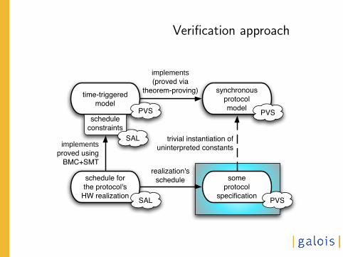
Verification approach

someprotocol

specification

schedule for the protocol's

HW realization

synchronous protocolmodel

implementsproved using

BMC+SMT

trivial instantiation ofuninterpreted constants

implements(proved via

theorem-proving)

PVSschedule

constraints

time-triggered model

PVS

SAL

SAL PVS

realization'sschedule

Synchronous specification

run(r , s)df=

if r = 0 then selse λp. transp(runp(r − 1, s),

λq. msgq(runq(r − 1, s), p)),where q ∈ in nbrsp

transp: state-transition function for node p.msgq: message-generation function for node q.in nbrsp: inbound-neighbor-nodes for node p.

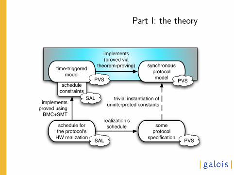
Part I: the theory

someprotocol

specification


HW realization



BMC+SMT



theorem-proving)

PVSschedule

constraints


PVS

SAL

SAL PVS


Part I: the theory

The theory Rushby built and I expanded upon is an axiomatic theory oftime-triggered protocols. The axioms fall into the following categories:

1. System assumptions (4 axioms)Assumptions made about the underlying clocks—e.g., clockmonotonicity, drift rate, skew bound, & communication delay.

2. Schedule constraints (6 axioms)Constraints on the local schedules—e.g., computation phase,communication phase, reception windows, & pipelining.

3. Semantics (9 axioms)The semantics of time-triggered behavior is a transition system,the states of which are (s, t) where s is the global state of thesystem and t is a realtime. The transitions between states areconstrained by the axioms.

The simulation theorem

Via taking “cuts” at regular points in time:

s0 −→ s1 −→ s2 → · · ·⇑ ⇑ ⇑

(s0, t) → · · · → (s1, t′) → · · · → (s2, t

′′) → · · ·

Part II: the implementation

someprotocol

specification


HW realization



BMC+SMT



theorem-proving)

PVSschedule

constraints


PVS

SAL

SAL PVS


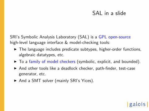
SAL in a slide

SRI’s Symbolic Analysis Laboratory (SAL) is a GPL open-sourcehigh-level language interface & model-checking tools:

I The language includes predicate subtypes, higher-order functions,algebraic datatypes, etc.

I To a family of model checkers (symbolic, explicit, and bounded).

I And other tools like a deadlock checker, path-finder, test-casegenerator, etc.

I And a SMT solver (mainly SRI’s Yices).

Verifying the schedules

1. The six schedule constraints are reformulated from PVS into SAL(nearly verbatim).

2. Schedules for the hardware are specified as simple infinite-statemachines (variables & constraints from the reals and integers).

I State variables include the round counter and schedule-variables(e.g., computation offset, communication offset, reception windowopening time, etc).

I State variables may be nondeterministically updated.

3. We prove the constraints using infinite-state bounded modelchecking via k-induction.k = number of rounds of the protocol.

Schedule constraints

1. Offset constraint 0 < P(r) < sched(r + 1)− sched(r).

2. Communication Constraint #1D(r) ≥ Σ(r) + Λ(r)− b(1− ρ) · (δnom − el)c.

3. Computation offset constraintP(r) > D(r) + Σ(r) + Λ(r) + d(1 + ρ) · (δnom + eu)e.

4. Pipeline constraint ¬independent(r) implies D(r) ≥ 0.

5. Communication constraint #2 r > 0 impliesD(r) ≥ P(r − 1)− sched(r) + sched(r − 1).

6. Reception window constraint0 ≤ R(r) ≤ D(r) + b(1− ρ) · (δnom − el)c − Σ(r)− Λ(r) + 1.

sched(r): clocktime round r begins.P(r): clocktime offset computation begins in round r .D(r): clocktime offset when communication begins in round r .Λ(r): maximum schedule discrepancy in round r .Σ(r): maximum clock skew in round r .

Verifying the schedules

1. The six schedule constraints are reformulated from PVS into SAL(nearly verbatim).

2. Schedules for the hardware are specified as simple infinite-statemachines (variables & constraints from the reals and integers).

I State variables include the round counter and schedule-variables(e.g., computation offset, communication offset, reception windowopening time, etc).

I State variables may be nondeterministically updated.

3. We prove the constraints using infinite-state bounded modelchecking via k-induction.k = number of rounds of the protocol.

Lessons (re)-learned

I Don’t be a verification purist! Or as J. Moore put it. . .

I Prove the consistency of your axioms (or hypotheses)!I Figure out what correctness means formally first (for

time-triggered systems, it’s “implementing a synchronousspecification”)!

I And then figure out what properties you need.I And then figure out how to implement it.

I Try out infinite-state bounded model checking (in SAL) forreal-time verification!

Quoting J. Moore

February 27, 2007, [email protected]

I think of theorem provers sort of like vehicles. What is thebest kind of vehicle to buy? Isn’t that silly question? Ifyou’re hauling kids to soccer practice, it might be a minivan.If you’re hauling hay to the cattle, it might be a pickup.

[email protected]

Lessons (re)-learned

I Don’t be a verification purist! Or as J. Moore put it. . .

I Prove the consistency of your axioms (or your hypotheses)!

I Figure out what correctness means formally first (fortime-triggered systems, it’s “implementing a synchronousspecification”)!

I A benefit of FV is to give engineers confidence that aggressiveoptimizations are provably correct.

I Try out infinite-state bounded model checking for real-timeverification!

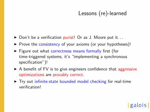
Towards a complete verification story

Abstraction levels:

I Application properties.

I Synchronous protocol abstraction.

I Time-triggered protocol abstraction.

I Real-time constraints.

I Distributed communicating state-machines.

I HW realization & physical-layer protocols.

}Miner et. al., FTRTFT’04}This paper}Schmaltz, FMCAD’07

Knapp&Paul, LNCS4444

SPIDER is open-spec and is a great testbench for new approaches!

Thanks

Steve Johnson, Paul Miner, Geoffrey Brown, Larry Moss, and WilfredoTorres-Pomales.

I was extraordinarily impressed with the thoroughness of myanonymous reviewers. Thanks!

Web resources

Slides, specifications, and proofs

http://www.cs.indiana.edu/∼lepike/pub pages/fmcad.htmlGoogle: lee pike fmcad

NASA SPIDER

http://shemesh.larc.nasa.gov/fm/spider/Google: spider nasa

PVS & SAL

http://fm.csl.sri.com/Google: formalware (please ignore tuxedo-related Google ads)

http://www.cs.indiana.edu/~lepike/pub_pages/fmcad.html

http://shemesh.larc.nasa.gov/fm/spider/

http://fm.csl.sri.com/

modeling time-triggered protocols and verifying their real

Documents