modeling two-phase transport during cryogenic chilldown in...
TRANSCRIPT

MODELING TWO-PHASE TRANSPORT DURING CRYOGENIC CHILLDOWN IN
A PIPELINE
By
JUN LIAO
A DISSERTATION PRESENTED TO THE GRADUATE SCHOOL OF THE UNIVERSITY OF FLORIDA IN PARTIAL FULFILLMENT
OF THE REQUIREMENTS FOR THE DEGREE OF DOCTOR OF PHILOSOPHY
UNIVERSITY OF FLORIDA
2005

Copyright 2005
by
Jun Liao

iii
ACKNOWLEDGMENTS
I would like to express my appreciation to all of the individuals who have assisted
me in my educational development and in the completion of my dissertation. My greatest
gratitude is extended to my supervisory committee chair, Dr. Renwei Mei. Dr. Mei’s
excellent knowledge, boundless patience, constant encouragement, friendly demeanor,
and professional expertise have been critical to both my research and education. Dr.
James F. Klausner also deserves recognition for his knowledge and technical expertise. I
would like to further thank Dr. Jacob N. Chung for kindly providing his experiment data
of chilldown.
I would like to additionally recognize my fellow graduate associates Christopher
Velat, Jelliffe Jackson, Yusen Qi, and Yi Li for their friendship and technical assistance.
Their diverse cultural background and character have provided an enlightening and
positive environment. Special appreciation is given to Kun Yuan for his kindness
providing his experiment data and insight on chilldown.
I would like to further acknowledge the Hydrogen Research and Education
Program for providing funding to this study. This research was also funded by NASA
Glenn Research Center under contract NAG3-2750.
Finally, I would like to recognize my wife Xiaohong Liao and my parents for their
continual support and encouragement.

iv
TABLE OF CONTENTS page ACKNOWLEDGMENTS.................................................................................................. iii
LIST OF TABLES ............................................................................................................vii
LIST OF FIGURES..........................................................................................................viii
NOMENCLATURE......................................................................................................... xiv
ABSTRACT..................................................................................................................... xix
CHAPTER 1 INTRODUCTION ....................................................................................................... 1
1.1 Background ............................................................................................................ 1 1.2 Literature Review................................................................................................... 4 1.3 Scope.................................................................................................................... 10
2 TWO-PHASE FLOW MODELING AND FLOW BOILING HEAT TRANSFER OF
CRYOGENIC FLUID................................................................................................ 13
2.1 Flow Regime and Heat Transfer Regime............................................................. 13 2.2 Flow Models in Cryogenic Chilldown................................................................. 18
2.2.1 Homogeneous Flow Model........................................................................ 18 2.2.2 Two-Fluid Model ....................................................................................... 22
2.3 Heat Transfer between Cryogenic Fluid and Solid Pipe Wall ............................. 26 2.3.1 Heat Transfer between Liquid and Solid wall ........................................... 27
2.3.1.1 Film boiling ..................................................................................... 27 2.3.1.2 Forced convection boiling and two-phase convective heat transfer 30
2.3.2 Heat Transfer between Vapor and Solid Wall ........................................... 33 3 VAPOR BUBBLE GROWTH IN SATURATED BOILING ................................... 34
3.1 Introduction.......................................................................................................... 34 3.2 Formulation.......................................................................................................... 39
3.2.1 On the Vapor Bubble ................................................................................. 39 3.2.2 Microlayer.................................................................................................. 41 3.2.3 Solid Heater ............................................................................................... 42

v
3.2.4 On the Bulk Liquid .................................................................................... 43 3.2.4.1 Velocity field ................................................................................... 43 3.2.4.2 Temperature field ............................................................................ 44 3.2.4.3 Asymptotic analysis of the bulk liquid temperature field during early
stages of growth ............................................................................... 46 3.2.5 Initial Conditions ....................................................................................... 50 3.2.6 Solution Procedure..................................................................................... 52
3.3 Results and Discussions ....................................................................................... 52 3.3.1 Asymptotic Structure of Liquid Thermal Field ......................................... 52 3.3.2 Constant Heater Temperature Bubble Growth in the Experiment of
Yaddanapudi and Kim............................................................................... 56 3.3.3 Effect of Bulk Liquid Thermal Boundary Layer Thickness on Bubble
Growth............................................................................................................. 59 3.4 Conclusions.......................................................................................................... 63
4 ANALYSIS ON COMPUTATIONAL INSTABILITY IN SOLVING TWO-FLUID
MODEL ..................................................................................................................... 64
4.1 Inviscid Two-Fluid Model ................................................................................... 65 4.1.1 Introduction................................................................................................ 65 4.1.2 Governing Equations ................................................................................. 67 4.1.3 Theoretical Analysis .................................................................................. 69
4.1.3.1 Characteristic analysis and ill-posedness ........................................ 69 4.1.3.2 Inviscid Kelvin-Helmholtz (IKH) analysis and linear instability.... 72
4.1.4 Analysis on Computational Instability ...................................................... 73 4.1.4.1 Description of numerical methods................................................... 73 4.1.4.2 Code validation— dam-break flow ................................................. 78 4.1.4.3 Von Neumann stability analysis for various convection schemes .. 81 4.1.4.4 Initial and boundary conditions for numerical solutions ................. 86
4.1.5 Results and Discussion .............................................................................. 87 4.1.5.1 Computational stability assessment based on von Neumann stability
analysis ............................................................................................. 87 4.1.5.2 Scheme consistency tests................................................................. 94 4.1.5.3 Computational assessment based on the growth of disturbance...... 95 4.1.5.4 Discussion on the growth of short wave........................................ 101 4.1.5.5 Wave development resulting from disturbance at inlet ................. 104
4.1.6 Conclusions.............................................................................................. 106 4.2 Viscous Two-Fluid Model ................................................................................. 110
4.2.1 Introduction.............................................................................................. 110 4.2.2 Governing Equations ............................................................................... 111 4.2.3 Theoretical Analysis ................................................................................ 112
4.2.3.1 Characteristics and ill-posedness................................................... 112 4.2.3.2 Viscous Kelvin-Helmholtz (VKH) analysis and linear instability 113
4.2.4 Analysis on Computational Intability ...................................................... 115 4.2.4.1 Description of numerical methods................................................. 115 4.2.4.2 Von Neumann stability analysis for various convection schemes 116 4.2.4.3 Initial and boundary conditions for numerical solution................. 119

vi
4.2.5 Results and Discussion ............................................................................ 119 4.2.5.1 Computational stability assessment based on von Neumann stability
analysis ........................................................................................... 119 4.2.5.2 Computational assessment based on the growth of disturbance.... 126 4.2.5.3 Wave development resulting from disturbance at inlet ................. 128
4.2.6 Conclusions.............................................................................................. 130 5 MODELING CRYOGENIC CHILLDOWN........................................................... 133
5.1 Homogeneous Chilldown Model ....................................................................... 133 5.1.1 Analysis ................................................................................................... 134 5.1.2 Results and Discussion ............................................................................ 136
5.2 Pseudo-Steady Chilldown Model....................................................................... 140 5.2.1 Formulation.............................................................................................. 141
5.2.1.1 Heat conduction in solid pipe ........................................................ 141 5.2.1.2 Liquid and vapor flow ................................................................... 144 5.2.1.3 Film boiling correlation ................................................................. 145 5.2.1.4 Forced convection boiling correlation ........................................... 151 5.2.1.5 Heat transfer between solid wall and environment........................ 152
5.2.2 Results and Discussion ............................................................................ 155 5.2.2.1 Experiment of Chung et al............................................................. 156 5.2.2.2 Comparison of pipe wall temperature ........................................... 157
5.2.3 Discussion and Remarks.......................................................................... 163 5.2.4 Conclusions.............................................................................................. 166
5.3 Separated Flow Chilldown Model ..................................................................... 167 5.3.1 Formulation.............................................................................................. 167
5.3.1.1 Fluid flow ...................................................................................... 168 5.3.1.2 Heat conduction in solid pipe ........................................................ 168 5.3.1.3 Heat and mass transfer................................................................... 169 5.3.1.3 Initial and boundary conditions ..................................................... 172
5.3.2 Solution Procedure................................................................................... 173 5.3.3 Results and Discussion ............................................................................ 174
5.3.3.1 Comparison of solid wall temperature........................................... 177 5.3.3.2 Flow field and fluid temperature ................................................... 181
5.3.4 Conclusions.............................................................................................. 186 6 CONCLUSIONS AND DISCUSSION ................................................................... 187
6.1 Conclusions........................................................................................................ 187 6.2 Suggested Future Study ..................................................................................... 188
LIST OF REFERENCES ................................................................................................ 190
BIOGRAPHICAL SKETCH .......................................................................................... 198

vii
LIST OF TABLES
Table page 4-1. Analytical solution for dam-break flow.................................................................... 80
4-2. ( )φ∆ for different discretization schemes.................................................................. 85
5-1. Heat and mass transfer relationship used in separated flow chilldown model. ....... 173

viii
LIST OF FIGURES
Figure page 1-1. Schematic of filling facilities for LH2 transport system from storage tank to space
shuttle external tank................................................................................................... 3
1-2. The schematic of chilldown and heat transfer regime. ................................................ 9
2-1. Schematic of two-phase flow regime in horizontal pipe. .......................................... 14
2-2. Schematic of two-phase flow regime in vertical pipe................................................ 14
2-4. Typical wall temperature variation during chilldown................................................ 17
2-5. Schematic for homogeneous flow model................................................................... 19
2-6. Schematic of the two-fluid model.............................................................................. 22
2-7. Schematic of heat transfer in chilldown..................................................................... 27
3-1. Sketch for the growing bubble, thermal boundary layer, microlayer and the heater wall. ......................................................................................................................... 39
3-2. Coordinate system for the background bulk liquid.................................................... 43
3-3. A typical grid distribution for the bulk liquid thermal field with 65.0=′RS ,
73.0=ψS , and 10=′∞R . .......................................................................................... 46
3-4. Comparison of the asymptotic and the numerical solutions at τ =0.001, 0.01, 0.1 and 0.3 for ψ=0°, 40°, and 71°. ..................................................................................... 54
3-5. Effect of parameter A on the liquid temperature profile near bubble. ....................... 55
3-6. The computed isotherms near a growing bubble in saturated liquid at τ=0.01, τ=0.1,τ=0.3, and τ=0.9. ........................................................................................... 57
3-7. Comparison of the equivalent bubble diameter eqd for the experimental data of Yaddanapudi and Kim (2001) and that computed for heat transfer through the microlayer ( 1c =3.0). ................................................................................................ 58
ix
3-8. Comparison of bubble diameter, d(t), between that computed using the present model and the measured data of Yaddanapudi and Kim (2001) ............................. 60
3-9. Comparison between heat transfer to the bubble through the vapor dome and that through the microlayer............................................................................................. 60
3-10. The computed isotherms in the bulk liquid corresponding to the thermal conditions reported by Yaddanapudi and Kim (2001). ............................................................. 61
3-11. Effect of bulk liquid thermal boundary layer thickness δ on bubble growth........... 62
4-1. Schematic of two-fluid model for pipe flow.............................................................. 68
4-2. Staggered grid arrangement in two-fluid model. ....................................................... 74
4-3. Flow chart of pressure correction scheme for two-fluid model................................. 78
4-4. Schematic for dam-break flow model........................................................................ 79
4-5. Water depth at t=50 seconds after dam break............................................................ 80
4-6. Water velocity at t=50 seconds after dam break........................................................ 81
4-7. Grid index number in staggered grid for von Neumann stability analysis. ............... 81
4-8. Comparisons of growth rates of various numerical schemes. 200=N , 5.0=la , smul /1= , smug /17= and 1.0=lCFL . .............................................................. 89
4-9. Growth rate of CDS scheme at different lg uuU −=∆ . 200=N , 5.0=la , smul /1= , and 1.0=lCFL . ................................................................................... 90
4-10. Growth rate of FOU scheme at different lg uuU −=∆ . 200=N , 5.0=la , smul /1= , and 1.0=lCFL . ................................................................................... 90
4-11. Growth rate of CDS scheme at different lu . 200=N , smU /16=∆ , 5.0=la , and msxt /1.0=∆∆ ....................................................................................................... 92
4-12. Growth rate of FOU scheme at different lu . 200=N , smU /16=∆ , 5.0=la , and msxt /1.0=∆∆ ....................................................................................................... 92
4-13. Growth rate of CDS scheme at different xt ∆∆ . 200=N , smul /1= , smU /16=∆ , and 5.0=la . ................................................................................... 93

x
4-14. Growth rate of FOU scheme at different xt ∆∆ . 200=N , smul /1= , smU /16=∆ , and 5.0=la . ................................................................................... 93
4-15. Comparison of lu growth using CDS scheme on different grids. smul /1= , smug /5.17= , 1.0=lCFL , and 5.0=la . ............................................................. 95
4-16. lu using CDS scheme in the computational domain. 200=N , smul /1= , smU /14=∆ , 05.0=lCFL , 5.0=la , and st 4= . ................................................ 97
4-17. Amplitude of liquid velocity disturbance lu using CDS scheme. 200=N , smul /1= , smU /14=∆ , 05.0=lCFL , 5.0=la , and st 4= .............................. 97
4-18. lu using CDS scheme after 10399 steps of computation, 200=N , smul /1= , smU /5.16=∆ , 1.0=lCFL , 5.0=la , and st 2.5= . ............................................ 98
4-19. Growth history of lu solved using CDS scheme, 200=N , smul /1= , smU /5.16=∆ , 1.0=lCFL , 5.0=la , and st 2.5= . ............................................ 98
4-20. Growth rate of FOU scheme, 200=N , smul /5.0= , smU /16=∆ , 02.0=lCFL , and 5.0=la . ......................................................................................................... 100
4-21. lu using FOU scheme after 12000 steps of computation. 200=N , smul /5.0= , smU /16=∆ , 02.0=lCFL , and 5.0=la . .................................... 102
4-22. Growth rate of SOU scheme. 200=N , smul /1= , smU /16=∆ , 05.0=lCFL , and 5.0=la . ......................................................................................................... 103
4-23. lu using SOU scheme after 3000 steps of computation. 200=N , smul /1= , smU /16=∆ , 05.0=lCFL , and 5.0=la . .......................................................... 103
4-24. Growth history of lu under different initial amplitude using FOU scheme........... 104
4-25. lu propagates in the pipe with FOU at well-posed condition, quasi-steady state. 107
4-26. lu propagates in the pipe with FOU scheme at ill-posed condition, quasi-steady state. ....................................................................................................................... 107
4-27. lu propagates in the pipe with CDS at well-posed condition, quasi-steady state. 108
4-28. lu propagates in the pipe with CDS at ill-posed condition, an instance before the computation breaks down. ..................................................................................... 108

xi
4-29. Comparison of growth rate between CDS and FOU schemes. 200=N , smul /1= , smug /21= , 05.0=lCFL , and 5.0=la . ............................................................ 109
4-30. Schematic depiction of viscous two-fluid model................................................... 111
4-31. Comparisons of growth rate of different schemes. 200=N , smuls /3.0= , smugs /6= ,and 1.0=lCFL ................................................................................. 120
4-32. Comparisons of growth rate of different schemes at low k. 200=N , smuls /3.0= , smugs /6= ,and 1.0=lCFL ................................................................................. 121
4-33. Growth rate for CDS scheme with VKH unstable. 200=N , smuls /3.0= , smugs /6= ,and 1.0=lCFL ................................................................................. 122
4-34. Growth rate for CDS scheme with VKH instability. sPawater *10 2−=µ , 200=N , smuls /3.0= , smugs /6= ,and 1.0=lCFL . ........................................................ 123
4-35. Growth rates for CDS scheme with VKH instability. sPawater *10 1−=µ , 200=N , smuls /1.0= , smugs /2= ,and 01.0=lCFL . ...................................................... 124
4-36. Growth rates for FOU scheme with VKH instability. 200=N , smuls /3.0= , smugs /6= , and 1.0=lCFL ................................................................................ 125
4-37. Growth rates for FOU scheme with VKH instability. sPaewater *11 −=µ , 200=N , smuls /1.0= , smugs /2= , and 01.0=lCFL . .................................... 125
4-38. Growth history of lu using CDS scheme. 200=N , smul /2= , smug /0.998174= , -0.0617144=β , 98.0=la , and 05.0=lCFL . .................. 127
4-39. Growth history of lu using FOU scheme. 200=N , smul /2= , smug /0.998174= , -0.0617144=β , 98.0=la , and 05.0=lCFL . .................. 128
4-40. Disturbance of lu propagates in the pipe with FOU and CDS schemes at VKH unstable and well-posed condition. ....................................................................... 129
4-41. Disturbance of lu propagates in the pipe with FOU and CDS schemes at both VKH unstable and well-posed condition. ....................................................................... 130
5-1. Schematic of homogeneous chilldown model. ........................................................ 134
5-2. Schematic for evaluating film boiling wall friction................................................. 135

xii
5-3. Distribution of vapor quality based on the homogenous flow model. ..................... 137
5-4. Pressure distribution based on the homogenous flow model................................... 138
5-5. Velocity distribution based on the homogenous flow model................................... 139
5-6. Solid temperature contour based on homogenous flow model. ............................... 139
5-7. Schematic of cryogenic liquid flow inside a pipe. ................................................... 141
5-8. Coordinate systems: laboratory frame is denoted using z; moving frame is denoted using Z. .................................................................................................................. 142
5-9. Schematic diagram of film boiling at stratified flow. .............................................. 145
5-10. Numerical solution of the vapor thickness and velocity influence functions. ....... 150
5-11. Numerical solution of ( )0ϕG ................................................................................. 151
5-12. Schematic of vacuum insulation chamber. ............................................................ 153
5-13. Schematic of Yuan and Chung (2004)’s cryogenic two-phase flow test apparatus.157
5-14. Experimental visual observation of Chung et al. (2004)’s cryogenic two-phase flow experiment. ............................................................................................................ 158
5-15. Computational grid arrangement and positions of thermocouples. ....................... 159
5-16. Comparison between measured and predicted transient wall temperatures of positions 12 and 15 at the bottom of pipe during film boiling chilldown. ............ 160
5-17. Comparison between measured and predicted transient wall temperatures of positions 12 and 15 at the bottom of pipe during convection boiling chilldown. . 161
5-18. Comparison between measured and predicted transient wall temperatures of positions 12 and 15 is at the bottom of pipe during entire chilldown. .................. 161
5-19. Comparison between measured and predicted transient wall temperatures of positions 11 and 14, which is at the bottom of pipe during entire chilldown........ 162
5-20. Cross section wall temperature distribution at t=0, 50, 100 and 300 seconds. ...... 162
5-21. Computed wall temperature contour on the inner surface of inner pipe................ 163
5-22. Comparison between measured and predicted transient wall temperatures of positions 12 and 15 with Chen correlation (1966). ............................................... 165
5-23. Schematic of separated flow chilldown model. ..................................................... 168

xiii
5-24. Schematic of heat and mass transfer in separated flow chilldown model. ............ 169
5-25. Flow chart of separated flow chilldown model...................................................... 175
5-26.Geometry of the test section and locations of thermocouples. ............................... 176
5-27. Comparison between measured and predicted transient wall temperatures of positions 12 and 15. ............................................................................................... 178
5-28. Comparison between measured and predicted transient wall temperatures of positions 11 and 14. ............................................................................................... 178
5-29. Comparison between measured and predicted transient wall temperatures of position 6 and 9 (the measured T 9 is obviously incorrect)................................... 179
5-30. Comparison between measured and predicted transient wall temperatures of positions 5 and 8. ................................................................................................... 179
5-31. Comparison between measured and predicted transient wall temperatures of position 3 and the numerical result of temperature at position 4........................... 180
5-32. Comparison between measured and predicted transient wall temperatures of positions 1 and 2. ................................................................................................... 180
5-33. Liquid nitrogen depth in the pipe during the chilldown. ....................................... 182
5-34. Vapor nitrogen velocity in the pipe during the chilldown. .................................... 183
5-35. Liquid nitrogen velocity in the pipe during the chilldown. ................................... 184
5-36. Vapor nitrogen temperature in the pipe during the chilldown............................... 185
5-37. Liquid nitrogen temperature in the pipe during the chilldown. ............................. 185

xiv
NOMENCLATURE
A dimensionless parameter for bubble growth, cross section area, surface area
Ab area of vapor bubble dome exposed to bulk liquid
Am area of wedge shaped interface
Bo Boiling number
c ratio of wedge shaped interface radius and vapor bubble radius, wave speed
1c microlayer wedge angle parameter; empirically determined
CFL Courant number
D diameter of pipe
lD and gD liquid layer and gas layer hydraulic diameter
d bubble diameter
eqd equivalent bubble diameter
E common amplitude factor
f friction factor
lof friction factor for liquid phase in homogeneous model
G mass flux, amplification factor
g gravity
lH and gH liquid layer and gas layer hydraulic depth
lh and gh liquid layer and gas layer depth

xv
h heat transfer coefficient
FBh film boiling heat transfer coefficient
poolh pool boiling heat transfer coefficient
clh , and cgh , forced convection heat transfer coefficient for liquid and gas
fgh latent heat of vaporization
I imaginary unit, 1−
i enthalpy
Ja Jacob number
k thermal conductivity, wavenumber
effk effective thermal conductivity
L local microlayer thickness, characteristic length
Nu Nusselt number
m′� mass transfer rate between liquid and gas per unit length
n normal direction
p pressure
0p pressure in the liquid-vapor interface
Pc Peclet number
Pr Prandtl number
q′ heat transfer rate per unit length
radq radiation heat flux
frcq free convection heat flux
wq ′′ Heat flux from wall to fluid

xvi
R vapor bubble radius, pipe radius
R� bubble growth rate
R′ ,ψ and ϕ spherical coordinates
R′ dimensionless radial coordinate
Rb radius of wedge shaped interface
0R initial bubble radius
Ra Rayleigh number
Re Reynolds number
r radial coordinate
S suppression factor in flow nucleate boiling, perimeter
RS ′ and ψS stretching factor in computation
T temperature
satT saturated temperature
wT initial solid temperature
bT bulk liquid temperature
t time
ct characteristic time
wt waiting period
0t initial time
U and V averaged velocities
u and v velocities
u mean u velocity

xvii
Vb vapor bubble volume
x, y, and z Cartesian coordinates
z, r, and ϕ cylindrical coordinates
X boundary layer coordinate
Z coordinate in the direction normal to the heating surface
Greek symbols
α thermal diffusivity, volume fraction
β volumetric thermal expansion coefficient
ttχ Martinelli number
T∆ solid wall superheat
δ superheated bulk liquid thermal boundary layer thickness, vapor film thickness
∗δ dimensionless thickness of unsteady thermal boundary layer
ε emissivity, amplitude
Φ velocity potential function for liquid flow, general variable
φ microlayer wedge angle, azimuthal coordinate, phase angle
loφ friction multiplier
η and ξ computational coordinates
λ characteristic root of a matrix
ν kinematic viscosity
θ dimensionless temperature, azimuthal coordinate, pipe incline angle
0θ initial dimensionless temperature of liquid
ρ density

xviii
σ stretched time in computation, Stefan Boltzmann constant
τ dimensionless time, shear stress
FBτ wall shear stress in film boiling regime
superscripts
in inner solution
out outer solution
‘ quantity per unit length
“ quantity per unit area
subscripts
b bubble
FB film boiling
eva evaporation
l, g, and i liquid, gas, and interface
i and o inner and outer pipe
l liquid
ml microlayer
NB nucleate boiling
w wall
v vapor
∞ far field condition

xix
Abstract of Dissertation Presented to the Graduate School of the University of Florida in Partial Fulfillment of the Requirements for the Degree of Doctor of Philosophy
MODELING TWO-PHASE TRANSPORT DURING CRYOGENIC CHILLDOWN IN A PIPELINE
By
Jun Liao
August 2005
Chair: Renwei Mei Major Department: Mechanical and Aerospace Engineering
Cryogenic chilldown process is a complicated interaction process among liquid,
vapor and solid pipe wall. To model the chilldown process, results from recent
experimental studies on the chilldown and existing cryogenic heat transfer correlations
were reviewed together with the homogeneous flow model and the two-fluid model. A
new physical model on the bubble growth in nucleate boiling was developed to correctly
predict the early stage bubble growth in saturated heterogeneous nucleate boiling. A
pressure correction algorithm for two-fluid model was carefully implemented to solve the
two-fluid model used to model the chilldown process. The connections between the
numerical stability and ill-posedness of the two-fluid model and between the numerical
stability and viscous Kelvin-Helmholtz instability were elucidated using von Neumann
stability analysis. A new film boiling correlation and a modified nucleate boiling
correlation for chilldown inside pipes were developed to provide heat transfer correlation
for chilldown model. Three chilldown models were developed. The homogeneous

xx
chilldown model is for simulating chilldown in a vertical pipe. A pseudo-steady
chilldown model was developed to simulate horizontal chilldown. The pseudo-steady
chilldown model can capture the essential part of chilldown process, provides a good
testing platform for validating cryogenic heat transfer correlations based on experimental
measurement of wall temperature during chilldown and gives a reasonable description of
the chilldown process in a frame moving with the liquid-vapor wave front. A more
comprehensive separated flow chilldown model was developed to predict both the flow
field and solid wall temperature field in horizontal stratified flow during chilldown. The
predicted wall temperature variation matches well with the experimental measurement. It
provides valuable insights into the two-phase flow dynamics, and heat and mass transfer
for a given spatial region in the pipe during the chilldown.

1
CHAPTER 1 INTRODUCTION
One of the key issues in the efficient utilization of cryogenic fluids is the transport,
handling, and storage of the cryogenic fluids. The complexity of the problems results
from, in general, the intricate interaction of the fluid dynamics and the boiling heat
transfer. Chilldown of the pipeline for transport cryogenic fluid is a typical example. It
involves unsteady two-phase fluid dynamics and highly transitory boiling heat transfer.
There is very little insight into the dynamic process of chilldown. This study will focus
on the understanding and modeling of the unsteady fluid dynamics and heat transfer of
the cryogenic fluids in a pipeline that is exposed to the atmospheric condition.
1.1 Background
Presently there exists considerable interest among U.S. Federal agencies in driving
the U.S. energy infrastructure with hydrogen as the primary energy carrier. The
motivation for doing so is that hydrogen may be produced using all other energy sources,
and thus using hydrogen as an energy carrier medium has the potential to provide a
robust and secure energy supply that is less sensitive to world fluctuations in the supply
of fossil fuels. The vision of building an energy infrastructure that uses hydrogen as an
energy carrier is generally referred to as the "hydrogen economy," and is considered the
most likely path toward widespread commercialization of hydrogen based technologies.
Hydrogen has the distinct advantage as fuel in that it has the highest energy density
of any fuel currently under consideration, 120 MJ/kg. In contrast, the energy density of
gasoline, which is considered relatively high, is approximately 44 MJ/kg. When

2
launching spacecraft, the energy density is a primary factor in fuel selection. When
considering liquid hydrogen to propel advanced aircraft turbo engines, it is a very
attractive option due to hydrogen’s high energy density. One drawback with using liquid
hydrogen as a fuel is that it’s volumetric energy capacity, 8.4 MJ/liter is about one
quarter that of gasoline, 33 MJ/liter. Therefore, liquid hydrogen requires more
volumetric storage capacity for a fixed amount of energy. Nevertheless, liquid hydrogen
is a leading contender as a fuel for both ground-based vehicles and for aircraft propulsion
in the hydrogen economy.
When any cryogenic system is initially started, (this includes turbo engines,
reciprocating engines, pumps, valves, and pipelines), it must go through a transient
chilldown period prior to operation. Chilldown is the process of introducing the
cryogenic liquid into the system, and allowing the hardware to cool down to several
hundred degrees below the ambient temperature. The chilldown process is anything but
routine and requires highly skilled technicians to chilldown a cryogenic system in a safe
and efficient manner.
A perfect example of utilization and chilldown cryogenic system exists in NASA’s
Kennedy Space Center (KSC). In the preparation for a space shuttle launch, liquid
hydrogen (as fuel) is filled from a storage tank to the main liquid hydrogen (LH2)
external tank (ET) through a complex pipeline system (Figure 1-1). The filling procedure
consists of 5 steps:
• Facility and orbiter chilldown. • Fill transition and initial fill (fill ET to 2%). • Fast fill ET (to 98%). • Fill ET (to 100%). • Replenish (maintain ET 100%).

3
Figure 1-1. Schematic of filling facilities for LH2 transport system from storage tank to
space shuttle external tank.
While the engineers have a general understanding of the process in the initial fill
and rapid fill stages, there has been very little insight about the process of chilldown,
which is the first procedure to be initiated. There is not a single formula or computer
code that can be used to estimate the elapse time during the chilldown stage if certain
operating condition changes. The absence of guidelines stems from our lack of
fundamental knowledge in the area of cryogenic chilldown. Many such engineering
issues are present in the transport, handling, and storage of cryogenic liquid in industry
applications.

4
1.2 Literature Review
Experimental studies: Studies on cryogenic chilldown started in the 1960s with the
development of rocket launching systems. Early experimental chilldown studies started in
the 1960s by Burke et al. (1960), Graham (1961), Bronson et al. (1962), Chi and Vetere
(1963), Steward (1970) and other researches. Burke et al. (1960) and Graham (1961)
experimentally studied the cryogenic chilldown in a horizontal pipe and in a vertical pipe,
respectively. However, none of these studies provided the flow regime information in
chilldown. Bronson et al. (1962) visually studied the flow regimes in a horizontal pipe
during chilldown with liquid hydrogen as the coolant. The results revealed that the
stratified flow is prevalent during the cryogenic chilldown.
Flow regimes and heat transfer regimes in the horizontal pipe chilldown were also
studied by Chi and Vetere (1963). Information on flow regimes was deduced by studying
the fluid temperature and the volume fraction during chilldown. Several flow regimes
were identified: single-phase vapor, mist flow, slug flow, annular flow, bubbly flow, and
single-phase liquid flow. Heat transfer regimes were identified as single-phase vapor
convection, film boiling, nucleate boiling, and single-phase liquid convection.
Recently, Velat et al. (2004) systematically studied cryogenic chilldown with
nitrogen in a horizontal pipe. Their study included: a visual recording of the chilldown
process in a transparent Pyrex pipe, which is used to identify the flow regime and heat
transfer regime; collecting temperature histories at different positions of the wall in
chilldown; and recording the pressure drop along the pipe. Chung et al. (2004) conducted
a similar study with nitrogen chilldown at relatively low mass flux and provided the data
needed to assess various heat transfer coefficients in the present study.

5
Modeling efforts: Burke et al. (1960) developed a crude chilldown model based on
1-D heat transfer through the pipe wall and the assumption of infinite heat transfer rate from
the cryogenic fluid to the pipe wall. The effects of flow regimes on the heat transfer rate
were neglected. Graham et al. (1961) correlated the heat transfer coefficient and pressure
drop with the Martinelli number (Martinelli and Nelson, 1948) based on their
experimental data. Chi (1965) developed a one-dimensional model for energy equations
of the liquid and the wall, based on the film boiling heat transfer between the wall and the
fluid. An empirical equation for predicting the chilldown time and the temperature was
proposed.
Steward (1970) developed a homogeneous flow model for cryogenic chilldown.
The model treated the cryogenic fluid as a homogeneous mixture. The continuity,
momentum and energy equations of the mixture were solved to obtain density, pressure
and temperature of mixture. Various heat transfer regimes were considered: film boiling,
nucleate boiling, and single-phase convection heat transfer. Careful treatment of different
heat transfer regimes resulted in a significant improvement in the prediction of the
chilldown time. The homogeneous mixture model was also employed by Cross et al.
(2002) who obtained a correlation for the wall temperature during chilldown with an
oversimplified treatment of the heat transfer between the wall and the fluid.
Similar efforts have been devoted to the study of the re-wetting problem, referred to
as cooling down of a hot object. Thompson (1972) analyzed the re-wetting of a hot dry
rod. The two-dimensional temperature profile inside the solid rod was numerically
calculated. The nucleate boiling heat transfer coefficient between the solid rod and the

6
liquid was simplified to a power law relation and the heat transfer in the film boiling
stage is neglected. The liquid temperature and velocity outside the rod are assumed to be
constant. Sun et al. (1974), and Tien and Yao (1975) solved similar problems and
obtained an analytical solution for the re-wetting. They considered different heat transfer
coefficients for flow boiling and single-phase convection in order to obtain more accurate
results for re-wetting problems. In those works the thermal field of the liquid is neglected
and the heat transfer coefficients at the boiling and the convection heat transfer stage are
over-simplified, and the results are only valid for the vertical outer surface of a rod or a
tube.
Chilldown in stratified flow regime, which is the prevalent in the horizontal
pipeline, was first studied by Chan and Banerjee (1981 a, b, c). They developed a
comprehensive separated flow model for the cool-down in a hot horizontal pipe. Both
phases were modeled with one-dimensional mass and momentum conservation equations.
The vapor and liquid phase mass and momentum equations were reduced to two wave
equations for the liquid depth and the velocity of the liquid. The energy equation for the
liquid was used to find the liquid temperature and energy equation of vapor phase was
neglected. The wall temperature was computed using a 2-dimensional transient heat
conduction equation and heat transfer in the radial direction was neglected. They also
tried to evaluate the position of onset of re-wetting by studying the instability of film
boiling. Their prediction for the wall temperature agreed well with their experimental
results. Although significant progress was made in handling the momentum equations,
the heat transfer correlations employed were not as advanced.

7
Following Chan and Banerjee’s (1981 a, b, c) separated flow model, Hedayatpour
et al. (1993) studied the cool-down in a vertical pipe with a modified separated flow
model. The flow regime is inverted annular film boiling flow, where the liquid core is
inside and the vapor film separates the cold liquid and the hot wall. This regime
frequently exists in cool-down in a vertical pipe. The modified separated flow model
retains the transient terms in the vapor momentum equation and the vapor phase energy
equation. The procedure is the following: first, the liquid mass conservation equation is
solved to obtain the liquid and vapor volume fractions. Then the vapor mass conservation
equation is used to solve the vapor velocity. The vapor momentum equation is
subsequently solved to obtain the vapor pressure. Finally, the liquid momentum equation
is employed to find the liquid velocity. The iteration stops when the solution is
converged. Although Chan and Banerjee (1981 a, b, c) and Hedayatpour et al. (1993)
were successful in the simulation of chilldown with the separated flow model, their
separated flow model is either incomplete or computationally inefficient.
c) Issues related to two-fluid model
The separated flow model is also called the two-fluid model, which consists of two
sets of conservation equations for the mass, momentum and energy of liquid and gas
phases. It was proposed by Wallis (1969), and further refined by Ishii (1975). Although
the two-fluid model is recognized as a useful computational model to simulate the
stratified multiphase flow in the pipeline, its application to the study of heat transfer in
two-phase flow in the pipeline is still limited.
The numerical scheme for the two-fluid model can be classified into two
categories. One is the compressible two-fluid model, which can be solved by a hyperbolic

8
equation solver. Examples are the commercial code OLGA (Bendikson et al., 1991),
Pipeline Analysis Code (PLAC) (Black et al., 1990) and Lyczkowski et al. (1978). The
other is the incompressible two-fluid model. Since the hyperbolic equation solver is not
applicable to incompressible two-fluid model, several approaches for incompressible
two-fluid model have emerged. One approach is to reduce the gas and liquid mass and
momentum equations to two wave equations for the liquid depth and velocity, such as in
Barnea and Taitel (1994b) and Chan and Banerjee (1991b). This treatment changed the
properties of two-fluid model. Hedayatpour et al. (1993) approach to two-fluid model is
not widely used due to lack of theoretical analysis on the convergence. Another approach
is to use the pressure correction method, which was initially introduced by Issa and
Woodburn (1998) and Issa and Kempf (2003) for the compressible two-fluid model.
Although their pressure correction scheme is powerful for simulating the multiphase flow
in the pipeline, the accuracy of the scheme is not reported. At the present, application of
pressure correction scheme on the multiphase flow with heat transfer in pipeline, such as
chilldown, does not exist.
d) Heat transfer in chilldown
A typical chilldown process involves several heat transfer regimes as shown in
Figure1-2. Near the liquid front is the film boiling regime. The knowledge of the heat
transfer in the film boiling regime is relatively limited, because i) film boiling has not
been the central interest in industrial applications; and ii) high temperature difference
causes difficulties in experimental investigations. For the film boiling on vertical
surfaces, early work was reported by Bromley (1950), Dougall and Rohsenow (1963) and
Laverty and Rohsenow (1967). Film boiling in a horizontal cylinder was first studied by

9
Bromley (1950); and the Bromley correlation was widely used. Breen and Westwater
(1962) modified Bromley’s equation to account for very small tubes and large tubes. If
the tube is larger than the wavelength associated with Taylor instability, the heat transfer
correlation is reduced to Berenson’s correlation (1961) for a horizontal surface.
Film boiling
Cryogenic Liquid
Liquid Front Wall
Nucleation boiling
Convective heat transfer
Vapor
X
Y
Figure 1-2. The schematic of chilldown and heat transfer regime.
Empirical correlations for cryogenic film boiling were proposed by Hendrick et al.
(1961, 1966), Ellerbrock et al. (1962), von Glahn (1964), Giarratano and Smith (1965).
These correlations relate a simple or modified Nusselt number ratio to the Martinelli
parameter. Giarratano and Smith (1965) gave detailed assessment of these correlations.
All these correlations are for steady state cryogenic film boiling. Their suitability for
transient chilldown applications is questionable.
When the pipe wall chills down further, film boiling ceases and nucleate boiling
occurs. It is usually assumed that the boiling switches from film boiling to nucleate
boiling right away instead of passing through a transition boiling regime. The position of
the film boiling transitioning to the nucleate boiling is often called re-wetting front,
because from that position the cold liquid starts touching the pipe wall. Usually the
Leidenfrost temperature indicates the transition from film boiling to nucleate boiling.

10
However, the Leidenfrost temperature is not steady, and varies under different flow and
thermal conditions (Bell, 1967). A recent approach is to check the instability of the vapor
film beneath the liquid core using Kelvin Helmholtz instability analysis (Chan and
Banerjee, 1981c).
Studies on forced convection boiling are extensive (Giarratano and Smith, 1965;
Chen, 1966; Bennett and Chen, 1980; Stephan and Auracher, 1981; Gungor and
Winterton, 1996; Zurcher et al., 2002). A general correlation for saturated boiling was
introduced by Chen (1966). Gungor and Winterton (1996) modified Chen’s correlation
and extended it to subcooled boiling. Enhancement and suppression factors for
macro-convective heat transfer were introduced. Gunger and Winterton’s correlation can
fit experimental data better than the modified Chen’s correlation (Bennett and Chen,
1980) and Stephan and Auracher correlation (1981). Recently, Zurcher et al. (2002)
proposed a flow pattern dependent flow boiling heat transfer correlation. This approach
improves the overall accuracy of heat transfer correlation by incorporating flow pattern.
Kutateladze (1952) and Steiner (1986) also provided correlations for cryogenic fluids in
pool boiling and forced convection boiling. Although they are not widely used, they are
expected to be more applicable for cryogenic fluids since the correlation was directly
obtained from cryogenic conditions. As the wall temperature drops further, boiling is
suppressed and the heat transfer is governed by two-phase convection; this is much easier
to deal with.
1.3 Scope
This dissertation focuses on understanding the unsteady fluid dynamics and heat
transfer of cryogenic fluids in a pipeline that is exposed to the atmospheric condition and
the corresponding solid heat transfer in the pipeline wall. Proper models for chilldown

11
simulation are developed to predict the flow fields, thermal fields, and residence time
during chilldown.
In Chapter 2, visualized experimental studies on heat transfer regimes and flow
regimes in cryogenic chilldown are reviewed. Based on the experimental observation,
homogeneous and separated flow models for the respectively vertical pipe and horizontal
pipe are discussed. The heat transfer models for the film boiling, flow boiling and forced
convection heat transfer in chilldown are reviewed and qualitatively assessed.
In Chapter 3, a physical model for vapor bubble growth in saturated nucleate
boiling is developed that includes both heat transfer through the liquid microlayer and
that from the bulk superheated liquid surrounding the bubble. Both asymptotic and
numerical solutions reveal the existence of a thin unsteady thermal boundary layer
adjacent to the bubble dome.
In Chapter 4, a pressure correction algorithm for two-fluid model is developed and
carefully implemented. Numerical stability of various convection schemes for both the
inviscid and viscous two-fluid model is analyzed. The connections between ill-posedness
of the two-fluid model and the numerical stability and between the viscous
Kelvin-Helmholtz instability and numerical stability are elucidated. The computational
accuracy of the numerical schemes is assessed.
In Chapter 5, a new film boiling coefficient is developed to accurately predict film
boiling heat flux for flow inside a pipe. The film boiling coefficient with the other
investigated heat transfer models are applied in building chilldown models. A
pseudo-steady chilldown model is developed to predict the chilldown time and the wall
temperature variation in a horizontal pipe in a reference frame that moves with the liquid

12
wave front. It is of low computational cost and allows for simple validation of the new
film boiling heat transfer correlations. A more comprehensive separated flow chilldown
model for the horizontal pipe is developed to predict the flow field of the liquid and vapor
and the temperature fields of the liquid, vapor and the solid wall in a fixed region of the
pipe flow. The unsteady development of the chilldown process for the vapor volume
fraction, velocities of the two-phases, and the temperatures of fluids and wall are
elucidated.
Chapter 6 concludes the research with a summary of the overall work and
discussion of the future works.

13
CHAPTER 2 TWO-PHASE FLOW MODELING AND FLOW BOILING HEAT TRANSFER OF
CRYOGENIC FLUID
Information of heat transfer regimes and flow regimes in cryogenic chilldown
obtained from the experimental study provides the foundation for modeling the heat
transfer and multiphase flow in chilldown. Based on the information of flow regimes,
corresponding flow models for simulating chilldown are discussed. For chilldown in the
vertical pipe, homogeneous flow model is preferred due to the prevalence of
homogeneous flow. For chilldown in the horizontal pipe, because the stratified flow is
prevalent, two-fluid model is adopted. The heat transfer models for film boiling, flow
boiling and forced convection heat transfer in chilldown are reviewed and qualitatively
assessed.
2.1 Flow Regime and Heat Transfer Regime
In the study of chilldown, one of the most important aspects of analysis is to
determine the type of flow regime in the given region of the pipe. The flow in cryogenic
chilldown is typically a two-phase flow, because liquid evaporates after a significant
amount of heat is transferred from the wall to the fluid during chilldown. The two-phase
flow regime is determined by many factors, such as fluid velocity, fluid density, vapor
quality, gravity, and pipe size. For horizontal flow, the flow regime is visually classified
as bubbly flow, plug flow, stratified flow, wavy flow, slug flow, and annular flow, as
shown in Figure 2-1. For vertical flow, the flow regimes include bubbly flow, slug flow,
churn flow, annular flow, as shown in Figure 2-2.

14
Figure 2-1. Schematic of two-phase flow regime in horizontal pipe.
BubbleFlow
SlugFlow
ChurnFlow
AnnualFlow
Figure 2-2. Schematic of two-phase flow regime in vertical pipe.

15
The cryogenic two-phase flow is characterized by low viscosity, small density ratio
of the liquid to the vapor, low latent heat of vaporization, and large wall superheat. For
example, the liquid viscosity, density ratio latent heat of saturated liquid to vapor, and
latent heat of the saturated water at 1 atm are 2.73E-4 Pa*s, 1610, 2256.8kJ/kg,
respectively, while the corresponding data for saturated hydrogen at 1 atm are1.36E-
5Pa*s, 37.9, 444kJ/kg. Furthermore, film boiling, which is prevalent during chilldown,
causes low wall friction. These factors combined with the complex interaction between
the momentum and the thermal transportation make the two-phase flow during the
chilldown to distinguish itself from ordinary two-phase flows.
In the visualized horizontal chilldown experiment by Velat et al. (2004), as shown
in Figure 2-3, the pressure in the liquid nitrogen Dewar drives the fluid. When the liquid
nitrogen first enters the test section, a film boiling front is positioned at the inlet of test
section. This film boiling front produces a significant evaporation accompanied by a high
velocity vapor front traversing down the test section. If the mixture velocity is high
enough due to the large pressure drop between the Dewar and the outlet of the test
section, a very fine mist of liquid is entrained in the vapor flow. Immediately behind the
film boiling front is a liquid layer attached to the wall. The flow regime is either the
stratified flow or annular flow, depending on the flow speed, the pipe size, and the fluid
properties. If the mixture velocity is high, the flow likely appears as annular flow,
otherwise stratified flow or wavy flow is more common. The visual observation shows
that the liquid droplets being entrained in stratified flow and wavy flow is insignificant.
The nucleate boiling front follows the film boiling, indicating the end of film
boiling and the cryogenic liquid starts contacting the wall. The position where the liquid

16
starts contacting the wall is affected by the wall super heat, the liquid layer velocity and
the thickness of the liquid layer. It is a complex hydrodynamic and heat transfer
phenomenon. Usually Leidenfrost temperature indicates the transition from film boiling
to nucleate boiling. If the wall temperature is lower than the Leidenfrost temperature, the
vapor film cannot sustain the weight of liquid layer and becomes unstable. Therefore, the
liquid starts contacting the wall, and film boiling ceases.
Once the liquid contacts the wall, the nucleate boiling starts. In the nucleate boiling
regime the heat transfer from the wall to the liquid is significantly larger than that in the
film boiling regime, and the wall is chilled down much faster, are shown in Figure 2-4. If
the nucleation sites are not completely suppressed, a region of rapid nucleate boiling is
seen at the quenching front. If most of nucleate sites are suppressed by the subcooled
liquid, the flow directly transforms to the forced convection heat transfer, and nucleate
boiling stage is not visible.
After the nucleate boiling stage, the chilldown process dramatically slows down as
the convection heat transfer dominates. The wall superheat is relatively low at this stage
but the heat leaking from the test section to the environment emerges. These factors lead
to a lower chilldown rate. In the meantime, the liquid gradually builds up in the pipe due
to less vapor generation and the friction between the liquid and the wall. The increase of
the liquid layer thickness eventually leads to the transition of the flow regimes. When the
liquid layer is thick enough, the stratified flow or wavy flow becomes unstable.
Eventually slugs are formed and the flow transforms to the slug flow. In the final stage of
chilldown, the flow is almost a single-phase liquid flow, occasionally with some small

17
slugs. In this stage, the chilldown is almost completed, and the pipe wall temperature
gradually reaches the liquid saturated temperature.
Figure 2-3. Schematics of observed flow structures in chilldown (Velat et al., 2004).
Figure 2-4. Typical wall temperature variation during chilldown. (Velat et al., 2004)
CryogenicLiquid
Film BoilingFront
Vapor Flow
CryogenicLiquid
Film BoilingRegion
Vapor Flow
Liquid Film Flow
Liquid Film FlowCryogenicLiquid Bubbly Flow
IncreasingTime
Nucleate Boiling Front

18
Chilldown in a vertical pipe is practically less important than the chilldown in
horizontal pipe, due to the fact that most of cryogenic transportation pipelines are
horizontal, and only a small part is vertical. The experimental study (Hedayapour et al.
1993; Laverty and Rohsenow, 1967) reveals that the flow regime is mainly bubble flow,
or inverted annular flow if the vapor film of the film boiling is stable, and single-phase
vapor flow and single-phase liquid flow exist at the beginning and the final stage of
chilldown, respectively.
2.2 Flow Models in Cryogenic Chilldown
Based on the experimental investigation, several flow regimes exist in cryogenic
chilldown. At different flow regimes, the models for evaluating velocity and volume
fraction of fluid are different. Two types of flow models are to be discussed in this
section. First is the homogeneous flow model, which is used for modeling the chilldown
in a vertical pipe, where the homogeneous flow is prevalent. Another model is the two-
fluid model, which is mostly used in simulating the stratified flow or wavy flow for the
chilldown in a horizontal pipe.
2.2.1 Homogeneous Flow Model
In the homogeneous flow model, the unsteady mass, momentum, and energy
conservation equations for the mixture are simultaneously solved. The primary
assumptions are: (1) single-phase fluid or two-phase mixture is homogeneous, and each
phase is incompressible; (2) thermal and mechanical equilibrium exists between the
liquid and the vapor flowing together; (3) flow is quasi-one-dimensional; and (4) axial
diffusion of momentum and energy is negligible.
Thus, the continuity equation for the mixture is

19
0)()( =∂
∂+∂
∂z
AutA ρρ , (2.1)
where ρ is the mixture density of liquid and vapor phase, u is the average fluid
velocity (by the assumption of homogeneous model, both liquid and vapor velocity are
u ), t is time , z is the vertical axial coordinate, and A is the cross section area of the
pipeline.
Mixture front
Pipe wall
Vapor bubble
Liquid
Figure 2-5. Schematic for homogeneous flow model.
By neglecting the viscous terms, the momentum equation for the mixture becomes
βρρρ sin)()(
f
gAAzpA
zp
zAuu
tAu ⋅−⋅
∂∂+
∂∂−=
∂∂+
∂∂ , (2.2)
where p is pressure,fz
P
∂∂ is the pressure drop due to wall friction, β is the inclination
angle of the pipe. For a vertical pipe, 2πβ = .
The energy equation for the homogeneous model is

20
Sqz
AiutAi
w′′=∂
∂+∂
∂ )()( ρρ , (2.3)
where i is the mixture enthalpy, wq ′′ is the heat flux from the wall to the fluid, and S is the
perimeter of the pipe.
If the cross section of the circular pipe is constant, the governing equations for
homogenous flow are simplified to the following equations.
0)()( =∂
∂+∂
∂zu
tρρ , (2.4)
θρρρ sin)()(
f
gzp
zp
zuu
tu −
∂∂+
∂∂−=
∂∂+
∂∂ , (2.5)
Aq
ziu
ti
wπρρ 4)()( ′′=
∂∂+
∂∂ . (2.6)
The pressure drop fz
P
∂∂ due to the wall friction is evaluated by the correlation for
the homogeneous system (Hewitt, 1982). In the correlation (Hewitt, 1982), a friction
multiplier 2loφ is defined as ratio of two-phase frictional pressure gradient
fzP
∂∂ to the
frictional pressure gradient for a single-phase flow at the same total mass flux and with
the physical properties of the liquid phase loz
P
∂∂ , i.e.
2lo
lo
f
dzdPdzdP
φ=
, (2.7)
where the friction multiplier 2loφ can be calculated by

21
25.0
2 11−
−+
−+=
g
gl
g
gllo xx
µµµ
ρρρ
φ , (2.8)
where subscribes l and g represent the liquid phase and gas phase, respectively. The
single-phase pressure drop loz
P
∂∂ is evaluated using the standard equation
l
lo
lo DGf
dzdP
ρ
22=
, (2.9)
where lof is the friction factor and for turbulent flow in a pipe, it is given as
25.0
079.0−
=
llo
GDfµ
. (2.10)
in which, G is the mixture mass flux.
Compared with the experimentally measured two-phase flow pressure drop, the
homogenous model tends to underestimate the value of two-phase frictional pressure
gradient (Klausner et al., 1990). However, it provides a reasonable lower bound of the
two-phase flow pressure drop.
In the film boiling regime, a layer of vapor film separates the liquid core from the
pipe wall. This vapor film significantly reduces the wall friction, so that the two-phase
flow pressure drop due to the friction is much lower than that in the other heat transfer
regimes. To date, no correlation for the friction coefficient in the film boiling regime
exists. In available chilldown studies, the vapor film is treated as a part of the mixture and
Martinelli type of pressure drop correlation is used, or the wall friction is simply set to
zero.

22
2.2.2 Two-Fluid Model
In the chilldown inside the horizontal pipe, it is assumed that flow is stratified and
the liquid and the vapor flow at different velocity (Figure 2-6). Two-fluid model (Willis,
1969; Ishii, 1975) is widely used to qualitatively investigate the stratified flow inside
horizontal pipeline with a relatively low computational cost compared with
2-dimensional or 3-dimensional fluid flow models. In the study of the horizontal pipe
chilldown, the fluid volume fractions, velocities, enthalpies are solved with the two-fluid
model.
Liquid layer U
Vapor layer
r
x
Wall heat flux
Pipe wall
D
Figure 2-6. Schematic of the two-fluid model.
The basis of the two-fluid model is a set of one-dimensional conservation equations
for the balance of mass, momentum and energy for each phase. The one-dimensional
conservation equations are obtained by integrating the flow properties over the
cross-sectional area of the flow.
In this study, it is assumed that flow is incompressible as the Mach number of the
gas phase is usually very low for the stratified flow. Hence, continuity equation for the
liquid phase (Chan and Banarjee, 1981c) is
( ) ( )l
lll Amu
xt ραα
′−=
∂∂+
∂∂ �
, (2.11)

23
where α is volume fraction, ρ is density, u is the velocity, t is the time, x is the axial
coordinate, and m′� is the mass transfer rate between the liquid phase and the gas phase
per unit length; the subscript l denotes liquid.
Similarly, continuity equation for the gas phase is
( ) ( )g
ggg Amu
xt ραα
′=
∂∂+
∂∂ D
, (2.12)
where the subscript g denotes gas. It is noted that
1=+ gl αα . (2.13)
The momentum equation for the liquid phase is
( ) ( )
,sincos
2
l
i
l
ii
l
lll
ll
i
l
lllll
Aum
AS
AS
gx
Hg
xp
ux
ut
ρρτ
ρτ
θαα
θ
ρααα
′−+−−
∂∂
−
∂∂
−=∂∂+
∂∂
�
(2.14)
where ip is the pressure at the liquid-gas interface, g is acceleration of gravity, β is the
angle of inclination of the pipe axis from the horizontal lane, τ is the shear stress, S is the
perimeter over which τ acts, A is the pipe cross section area, lH is the liquid phase
hydraulic depth; the subscript i denotes liquid-gas interface. The second term on the right
hand side of Equation (2.14) represents the effect of gravity on the wavy surface of liquid
layer. The liquid phase hydraulic depth lH is defined as
l
l
ll
ll h
Hαα
αα
′=
∂∂= , (2.15)
where lh is the liquid layer depth.
Similarly, the momentum equation for the gas phase is

24
( ) ( )
,sincos
2
g
i
g
ii
g
ggg
lg
i
g
ggggg
Aum
AS
AS
gx
Hg
xp
ux
ut
ρρτ
ρτ
θαα
θ
ρα
αα
′+−−−
∂∂
−
∂∂
−=∂∂+
∂∂
D
(2.16)
where gH is the gas phase hydraulic depth. It is defined as
g
g
gg
gg h
Hαα
αα
′=
∂∂= , (2.17)
where gh is the gas layer thickness.
To study heat transfer, appropriate energy equations for both phases are required in
the two-fluid model. Similar to the assumptions made in the homogeneous flow model,
the heat conduction inside the fluid is neglected. Thus the one-dimensional energy
equations for the liquid phase and the gas phase are
( ) ( )l
l
l
illlll A
qA
imiu
xi
t ρραα
′+
′−=
∂∂+
∂∂ �
, (2.18)
and
( ) ( )g
g
g
iggggg A
qA
imiux
it ρρ
αα′
+′
=∂∂+
∂∂ �
, (2.19)
where i is enthalpy, and q′ is the heat transfer rate to the fluid per unit length.
In the two-fluid model, shear stresses lτ , gτ and iτ must be specified to close the
two fluid model. There are many correlations for shear stresses for separated flow model,
such as those developed by Wallis (1946), Barnea and Taitel (1976), and Andritsos and
Hanratty (1987). No significant difference exists among these models except at the flow
regime transition and at the high-speed flow, which will not be addressed in this study.

25
Thus, widely accepted shear stress correlations by Barnea and Taitel (1994) are
employed:
2
2ll
llUf ρτ = , (2.20)
2
2gg
gg
Uf
ρτ = , (2.21)
( )2
lglgii
UUUUf
−−=τ , (2.22)
where τ is shear stress, subscripts l, g, and i represent interface between the liquid and the
wall, interface between the gas and the wall, interface between the liquid and gas,
respectively. Friction factors f are given by
nlll Cf −= Re , and m
ggg Cf −= Re , (2.23)
where lRe is defined as
l
llll
DUµ
ρ=Re , (2.24)
where lD is the liquid hydraulic diameter
l
ll S
AD
4= , (2.25)
in which lA is liquid phase cross section area, lS is the liquid phase perimeter. In
Equation (2.23) gRe is defined as
g
gggg
DUµ
ρ=Re , (2.26)
where gD is vapor phase hydraulic diameter

26
iv
gg SS
AD
+=
4 (2.27)
in which gA is vapor phase cross section area, gS is the vapor phase perimeter, and iS is
the liquid-gas interface perimeter.
The coefficients gC and lC are equal to 0.046 for turbulent flow and 16 for
laminar flow, while n and m take the values of 0.2 for turbulent flow and 1.0 for laminar
flow. The interfacial friction factor is assumed to be gi ff = or 014.0=if , if
014.0<gf .
It is supposed that this model works in the flow boiling regime and in the forced
convection heat transfer regime. However, in the film boiling stage, presence of vapor
film dramatically reduces the shear stress between the liquid and the wall. In such a
situation, lτ should be evaluated to include the effect of vapor film layer.
2.3 Heat Transfer between Cryogenic Fluid and Solid Pipe Wall
During cryogenic chilldown, the fluid in contact with the pipe wall is either the
liquid or the vapor. The mechanisms of heat transfers between the liquid and the wall and
between the vapor and the wall are different, as shown in Figure 2-7. Based on
experimental measurements and theoretical analysis, liquid-solid heat transfer accounts
for a majority of the total heat transfer. However, the liquid-solid heat transfer is much
more complicated than the heat transfer between the vapor and the wall due to occurrence
of film boiling and nucleate boiling. Thus, the heat transfer between the liquid and the
wall is discussed first.

27
2.3.1 Heat Transfer between Liquid and Solid wall
The heat transfer mechanism between the liquid and the solid wall includes film
boiling, nucleate boiling, and two-phase convection heat transfer. The transition from one
type of heat transfer to another depends on many parameters, such as the wall
temperature, the wall heat flux, and properties of the fluid. For simplicity, a fixed
temperature approach is adopted to determine the transition point. That is, if the wall
temperature is higher than the Leidenfrost temperature, film boiling is assumed. If the
wall temperature is between the Leidenfrost temperature and a transition temperature, T2,
nucleate boiling is assumed. If the wall temperature is below the transition temperature
T2, two-phase convection heat transfer is assumed. The values of the Leidenfrost
temperature and the transition temperature are determined by matching the model
prediction with the experimental results.
Film boiling Flow boiling Convective heat transfer (liquid)
Liquid layer
Vapor layer Convective heat transfer (vapor)
Liquid
Vapor
Wall heat flux
Pipe wall
D
Thin vapor film
Figure 2-7. Schematic of heat transfer in chilldown.
2.3.1.1 Film boiling
Due to the high wall superheat encountered in the cryogenic chilldown, film boiling
plays a major role in the heat transfer process in terms of the time span and in terms of

28
the total amount of heat removed from the wall, as shown in Figure 2-4. Currently there
exists no specific film boiling correlation for chilldown applications with such high wall
superheat. The research starts from the conventional film boiling correlations.
A cryogenic film boiling heat transfer correlations was provided by Giarratano and
Smith (1965),
)(* 4.0tt
calc
fBoNu
Nu χ=
− , (2.28)
where Nu is Nusselt number
l
FB
kDhNu *
= , (2.29)
where FBh is the film boiling heat transfer coefficient and lk is the thermal conductivity
of the liquid, Bo is the boiling number
Gh
qBofg *
= , (2.30)
where fgh is the evaporative latent heat of the fluid. In Equation (2.28), calcNu is the
Nusselt number for the two-phase convection heat transfer, which can be obtained using
4.08.0 Pr*Re*023.0=calcNu , (2.31)
where Re is Reynolds number of mixture and Pr is Prandtl number of vapor, ttχ is
Martinelli number
1.05.09.01
−=v
l
l
vtt x
xµµ
ρρχ . (2.32)
In Giarratano and Smith (1965) correlation, the heat transfer coefficient is the
averaged value for the whole cross section. Similar correlations for cryogenic film

29
boiling also exist in the literature. The correlations were obtained from measurements
conducted under steady state. The problem with the use of these steady state film boiling
correlations is that they do not account for information of flow regimes. For example, for
the same quality, the heat transfer rate for annular flow is much different from that for
stratified flow. Available empirical correlations do not make such difference.
Furthermore, in this study, local heat transfer coefficient is needed in order to
incorporate the thermal interaction with the pipe wall. Since the two-phase flow regime
information is available in the present study through the visualized experiment, it is
expected that the modeling effort should take into account the knowledge of the flow
regime. Suppose a liquid-gas stratified flow exists inside a horizontal pipe. Due to
gravity, the upper part of pipe wall is in contact with the gas, and lower part of pipe wall
is in contact with the flowing liquid. Thus, the heat transfer coefficient on upper wall is
significantly different from that on the lower wall. Apparently, the local heat transfer
coefficient strongly depends on the local flow condition instead an overall parameter such
as the flow quality at the given location.
There are several correlations for the film boiling based on the analysis of the vapor
film boundary layer, such as Bromley correlation (1950) and Breen and Westerwater
correlation (1962) for film boiling on the outer surface of a hot tube. Frederking and
Clark (1965) and Carey (1992) correlations, for the film boiling on the surface of a
sphere, are included as well. However, none of these was obtained for cryogenic fluids or
for the film boiling on the inner surface of a pipe or tube.

30
2.3.1.2 Forced convection boiling and two-phase convective heat transfer
A pool boiling correlation for cryogens was proposed by Kutateladze (1952). The
pool nucleated boiling heat transfer coefficient poolh is
( )
( )5.1
626.0906.05.1
5.1,
750.1282.110 *10*487.0 T
hcpk
hlvfg
lpllpool ∆
= −
µσρρ
, (2.33)
where σ is liquid surface tension, µ is viscosity, and ∆T is wall superheat. Based on this
pool boiling correlation, a convection boiling correlation was proposed (Giarratano and
Smith, 1965). The heat transfer coefficient is contributed by both convection heat transfer
and ebullition:
poolcl hhh += , , (2.34)
where clh , is given by Dittus-Boelter equation which is used in fully developed pipe
flow:
llllcl Dkh /PrRe*023.0 4.08.0, = , (2.35)
where lRe is defined as
ll
DGµ
=Re . (2.36)
Chen (1966) introduced enhancement factor E and suppression factor S into the
flow boiling correlation. The heat transfer coefficient is given
poolcl ShEhh += , . (2.37)
Enhancement factor E reflects the much higher velocities and hence forced convection
heat transfer in the two-phase flow compared to the single-phase, liquid only flow. The
suppression factor S reflects the lower effective superheat in the forced convection as
opposed to pool boiling, due to the thinner boundary condition. The value of E and S are

31
presented as graphs in Chen (1966). The pool boiling heat transfer coefficient in Chen
correlation is
75.024.024.024.029.05.0
25.049.045.0,
79.0
00122.0 PTh
gckh
vfg
llclpool ∆∆
=
ρµσρ
. (2.38)
Chen correlation (1966) fits best for annular flow since it was developed for vertical
flows. For the stratified flow regime, Chen’s correlation may not be applicable.
At the flow boiling heat transfer, Gungor and Winterton correlation (1996) is
widely used due to that it fits much more experimental data. The basic form of Gungor
and Winterton correlation is similar to Chen correlation (1966), Equation (2.37).
However, evaluation of E and S in Gungor and Winterton’s correlation takes account for
the influence of heat transfer rate by adding boiling number Bo. Thus, E and S are
presented as
( ) 86.016.1 /137.1240001 ttBoE χ++= , (2.39)
and
17.126 Re1015.111
lES −×+= . (2.40)
The pool boiling correlation implemented is proposed by Cooper (1984)
( ) 67.05.055.010
12.0 log55 qMPPh rrpool−−−= (2.41)
The solution of heat transfer correlation in Gungor and Winterton’s correlation is
implicitly obtained by iteration.
Although Gungor and Winterton correlation (1996) is widely used due to its good
agreement with a large data set, a closer examination on this correlation shows that it is
based mainly on the following parameters: Pr, Re, and quality x. Similar to the

32
development of conventional film boiling correlations, these parameters all reflect overall
properties of the flow in the pipe and are not directly related to flow regimes. Thus, it
cannot be used to predict the local heat transfer coefficients required in chilldown
simulation.
Most of existing force convection boiling heat transfer correlations do not
effectively take account the influence of flow regimes and flow patterns. Recently,
Zurcher et al. (2002) proposed a flow pattern dependent heat transfer correlation for the
horizontal pipe. The strategy employed in Zurcher et al. (2002) is that the flow pattern is
obtained using the flow pattern map at the first step. The information of flow pattern
determines the part of wall contacting with the liquid or the vapor, then corresponding
conventional heat transfer correlations is employed to determine the local heat transfer
coefficient. The heat transfer coefficient for the whole pipe is obtained by averaging the
local heat transfer coefficient along the perimeter of the pipe. Although details of the
approach like flow pattern map, and correlations employed are not perfect in study of
Zurcher et al. (2002), their approach to the flow boiling heat transfer is intelligible and
provides insight for studying chilldown.
When wall superheat drops to a certain range all the nucleation sites are suppressed.
The heat transfer is dominated by two-phase forced convection. The heat transfer
coefficient can then be predicated using Equation (2.35), when the flow is turbulent, or
Equation (2.42), when the flow is laminar.
llcl Dkh /*36.4, = . (2.42)

33
2.3.2 Heat Transfer between Vapor and Solid Wall
The heat transfer between the vapor and wall can be estimated by treating the flow
as a fully developed forced convection flow, neglecting the liquid droplets that are
entrapped in the vapor. The heat transfer coefficient of vapor forced convective flow is
ggggcg Dkh /PrRe*023.0 4.08.0, = , (turbulent flow) (2.43)
ggcg Dkh /*36.4, = , (laminar flow) (2.44)

34
CHAPTER 3 VAPOR BUBBLE GROWTH IN SATURATED BOILING
Accurate evaluation of the nucleate boiling coefficient is a critical part of the study
on the chilldown process because it provides the heat transfer rate from the wall to the
cryogenic fluid. During the nucleate boiling the vapor bubble growth rate has a directly
influence on the heat transfer rate. The higher the bubble growth rate, the higher the heat
transfer rate. A physical model for vapor bubble growth in saturated nucleate boiling has
been developed that includes both heat transfer through the liquid microlayer and that
from the bulk superheated liquid surrounding the bubble. Both asymptotic and numerical
solutions for the liquid temperature field surrounding a hemispherical bubble reveal the
existence of a thin unsteady thermal boundary layer adjacent to the bubble dome. During
the early stages of bubble growth, heat transfer to the bubble dome through the unsteady
thermal boundary layer constitutes a substantial contribution to vapor bubble growth. The
model is used to elucidate recent experimental observations of bubble growth and heat
transfer on constant temperature microheaters reported by Yaddanapudi and Kim (2001)
and confirms that the heat transfer through the bubble dome can be a significant portion
of the overall energy supply for the bubble growth.
3.1 Introduction
During the past forty years, the microlayer model has been widely accepted and
used to explain bubble growth and the associated heat transfer in heterogeneous nucleate
boiling. The microlayer concept was introduced by Moore and Mesler (1961), Labunstov
(1963) and Cooper (1969). The microlayer is a thin liquid layer that resides beneath a

35
growing vapor bubble. Because the layer is quite thin, the temperature gradient and the
corresponding heat flux across the microlayer are high. The vapor generated by strong
evaporation through the liquid microlayer substantially supports the bubble growth.
Popular opinion concerning the microlayer model is that the majority of
evaporation takes place at the microlayer. A number of bubble growth models using
microlayer theory have been proposed based on this assumption such as van Stralen et al.
(1975), Cooper (1970), and Fyodrov and Klimenko (1989). These models were partially
successful in predicting the bubble growth under limited conditions but are not applicable
to a wide range of conditions. Lee and Nydahl (1989) used a finite difference method to
study bubble growth and heat transfer in the microlayer. However their model assumes a
constant wall temperature, which is not valid for heat flux controlled boiling since the
rapidly growing bubble draws a substantial amount of heat from the wall through the
microlayer, which reduces the local wall temperature. Mei et al. (1995a, 1995b)
considered the simultaneous energy transfer among the vapor bubble, liquid microlayer,
and solid heater in modeling bubble growth. For simplicity, the bulk liquid outside the
microlayer was assumed to be at the saturation temperature so that the vapor dome is at
thermal equilibrium with the surrounding bulk liquid. The temperature in the heater was
determined by solving the unsteady heat conduction equation. The predicted bubble
growth rates agreed very well with those measured over a wide range of experimental
conditions that were reported by numerous investigators. Empirical constants to account
for the bubble shape and microlayer angle were introduced.
Recently, Yaddanapudi and Kim (2001) experimentally studied single bubbles
growing on a constant temperature heater. The heater temperature was kept constant by

36
using electronic feed back loops, and the power required to maintain the temperature was
measured throughout the bubble growth period. Their results show that during the bubble
growth period, the heat flux from the wall through the microlayer is only about 54% of
the total heat required to sustain the measured growth rate. It poses a new challenge to
the microlayer theory since a substantial portion of the energy transferred to the bubble
cannot be accounted for.
Since a growing vapor bubble consists of a thin liquid microlayer, which is in
contact with the solid heater, and a vapor dome, which is in contact with the bulk liquid,
the experimental observations of Yaddanapudi and Kim (2001) leads us to postulate that
the heat transfer through the bubble dome may play an important role in the bubble
growth process, even for saturated boiling. Because the wall is superheated, a thermal
boundary layer exists between the background saturated bulk liquid and the wall; within
this thermal boundary layer the liquid temperature is superheated. During the initial stage
of the bubble growth, because the bubble is very small in size, it is completely immersed
within this superheated bulk liquid thermal boundary layer. As the vapor bubble grows
rapidly, a new unsteady thermal boundary layer develops between the saturated vapor
dome and the surrounding superheated liquid. The thickness of the new unsteady thermal
boundary layer should be inversely related to the bubble growth rate; see the asymptotic
analysis that follows. Hence the initial rapid growth of the bubble, which results in a thin
unsteady thermal boundary layer, is accompanied by a substantial amount of heat transfer
from the surrounding superheated liquid to the bubble through the vapor bubble dome.
This is an entirely different heat transfer mechanism than that associated with
conventional microlayer theory.

37
In fact, many previous bubble growth models have attempted to include the
evaporation through the bubble dome, such as Han and Griffith (1965) and van Stralen
(1967). However their analyses neglected the convection term in the bulk liquid due to
the bubble expansion, so the unsteady thermal boundary layer was not revealed. This
leads to a much lower heat flux through the bubble dome.
The existence and the analysis on the unsteady thermal boundary layer near the
vapor dome were first discussed in Chen (1995) and Chen et al. (1996), when they
studied the growth and collapse of vapor bubbles in subcooled boiling. For subcooled
boiling, the effect of heat transfer through the dome is much more pronounced due to the
larger temperature difference between the vapor and the bulk liquid. With the presence
of a superheated wall, a subcooled bulk liquid, and a thin unsteady thermal boundary
layer at the bubble dome, the folding of the liquid temperature contour near the bubble
surface was observed in their numerical solutions. The folding phenomenon was
experimentally confirmed by Mayinger (1996) using an interferometric method to
measure the liquid temperature.
Despite those findings, the existence of the thin unsteady thermal boundary layer
near the bubble surface has not received sufficient attention. In the recent computational
studies of bubble growth by Son et al. (1999) and Bai and Fujita (2000), the conservation
equations of mass, momentum, and energy were solved in the Eulerian or
Lagrange-Eulerian mixed grid system for the vapor-liquid two-phase flow. In their direct
numerical simulations of the bubble growth process, the heat transfer from the
surrounding liquid to the vapor dome is automatically included since the integration is
over the entire bubble surface. They observed that there could be a substantial amount of

38
heat transfer though bubble dome in comparison with that from the microlayer.
However, it is not clear that if these direct numerical simulations have sufficiently
resolved the thin unsteady thermal boundary layer that is attached to the rapidly growing
bubble.
In this study, asymptotic and numerical solutions to the unsteady thermal fields
around the vapor bubble are presented. The structure of the thin, unsteady thermal
boundary layer around the vapor bubble is elucidated using the asymptotic solution for a
rapidly growing bubble. A new computational model for predicting heterogeneous
bubble growth in saturated nucleate boiling is presented. The model accounts for energy
transfer from the solid heater through the liquid microlayer and from the bulk liquid
through the thin unsteady thermal boundary layer on the bubble dome. It is equally valid
for subcooled boiling, although the framework for this case has already been presented by
Chen (1995) and Chen et al. (1996). The temperature field in the heater is simultaneously
solved with the temperature in the bulk liquid. For the microlayer, an instantaneous linear
temperature profile is assumed between the vapor saturation temperature and the heater
surface temperature due to negligible heat capacity in the microlayer. For the bulk liquid,
the energy equation is solved in a body-fitted coordinate system that is attached to the
rapidly growing bubble with pertinent grid stretching near the bubble surface to provide
sufficient numerical resolution for the new unsteady thermal boundary layer. Section 3.2
presents a detailed formulation of the present model and an asymptotic analysis for the
unsteady thermal boundary layer. In Section 3.3, the experimental results of
Yaddanapudi and Kim (2001) are examined using the computational results based on the

39
present model. A parametric investigation considering the effect of the superheated bulk
liquid thermal boundary layer thickness on bubble growth is also presented.
3.2 Formulation
3.2.1 On the Vapor Bubble
Consideration is given to an isolated vapor bubble growing from a solid heating
surface into a large saturated liquid pool, as shown in Figure 3-1. A rigorous description
of the vapor bubble growth and the heat transfer processes among three phases requires a
complete account for the hydrodynamics around the rapidly growing bubble in addition
to the complex thermal energy transfer. The numerical analysis by Lee and Nydahl
(1989) relied on an assumed shape for the bubble, although the hydrodynamics based on
the assumed bubble shape is properly accounted for. Son et al. (1999) and Bai and Fujita
(2000) employed the Navier-Stokes equations and the interface capture or trace methods
to determine the bubble shape. Nevertheless, the microlayer structure was still assumed
based on existing models.
ψ φ
R(t)
Solid wall;heat issupplied from
within or below
Backgroundbulk liquid
Bulk liquidthermal boundary
layer
Liquidmicrolayer
z
ψ
Figure 3-1. Sketch for the growing bubble, thermal boundary layer, microlayer and the
heater wall.

40
In this study, the liquid microlayer between the vapor bubble and the solid heating
surface is assumed to have a simple wedge shape with an angle φ<<1. The interferometry
measurements of Koffman and Plesset (1983) demonstrate that a wedge shape microlayer
is a good assumption. There exists ample experimental evidence by van Stralen (1975)
and Akiyama (1969) that as a bubble grows, the dome shape may be approximated as a
truncated sphere with radius )(tR , as shown in Figure 3-1. Using cylindrical coordinates,
the local microlayer thickness is denoted by )(rL . The radius of the wedge-shaped
interface is denoted by )(tRb , which is typically not equal to )(tR . Let
)(/)( tRtRc b= , (3.1)
and the vapor bubble volume )(tVb can be expressed as
)()(3
4)( 3 cftRtVbπ= ,
(3.2)
where )(cf depends on the geometry of the truncated sphere. In the limit 1→c , the
bubble is a hemisphere and )()3/2()( 3 tRtVb π→ . In the limit 0→c , the bubble
approaches a sphere and )()3/4()( 3 tRtVb π→ .
To better focus the effort of the present study on understanding the complex
interaction of the thermal field around the vapor dome, additional simplification is
introduced. The bubble shape is assumed to be hemispherical (c=1) during the growth.
Comparing with the direct numerical simulation technique which solves bubble shape
and fluid velocity field using Navier-Stokes equation, this simplification introduces some
error in the bubble shape and fluid velocity and temperature fields in this study. However,
the hemispherical bubble assumption is generally valid at high Jacob number nucleate
boiling (Mei, et al. 1995a) and at the early stage of low Jacob number bubble growth

41
(Yaddanapudi and Kim, 2001). A more complete model that incorporates the bubble
shape variation could have been used, as in Mei et al. (1995a); however, the present
model allows for a great simplification in revealing and presenting the existence and the
effects of a thin unsteady liquid thermal boundary layer adjacent to the bubble dome and
the influence of bulk liquid thermal boundary layer on saturated nucleate boiling. The
present simplified model is not quantitatively valid when the shape of the vapor bubble
deviates significantly from a hemisphere.
The energy balance at the liquid-vapor interface for the growing bubble depicted in
Figure 3-1 is described as
∫∫=′= ∂
∂−+
∂∂
−= btRR
llm
rLz
mll
bfgv dA
nT
kdAn
Tk
dtdV
h)()(
ρ , (3.3)
where vρ is the vapor density, fgh is the latent heat, lk is the liquid thermal conductivity,
Tl is the temperature of the bulk liquid, Tml is the temperature of the microlayer liquid, Am
is the area of wedge, Ab is the area of the vapor bubble dome exposed to bulk liquid, n∂∂
is the differentiation along the outward normal at the interface, and R′ is the spherical
coordinate in the radial direction attached to the moving bubble. Equation (3.3) simply
states that the energy conducted from the liquid to the bubble is used to vaporize the
surrounding liquid and thus expand the bubble.
3.2.2 Microlayer
The microlayer is assumed to be a wedge centered at 0=r with local thickness
)(rL . Because the hydrodynamics inside the microlayer are not considered, the
microlayer wedge angle φ cannot be determined as part of the solution. In Cooper and
Lloyd (1969), the angle φ was related to the viscous diffusion length of the liquid as

42
tctR lb νφ 1tan)( = in which lν is the kinematic viscosity of the liquid. A small φ
results in
)(1
tRtc
b
lνφ = . (3.4)
Cooper and Lloyd (1969) estimated 1c to be within 0.3-1.0 for their experimental
conditions.
A systematic investigation for saturated boiling by Mei et al. (1995b) established
that the temperature profile in the liquid microlayer can be taken as linear for practical
purposes. The following linear liquid temperature profile in the microlayer is thus
adopted in this study
( ) ( ) ( )
−∆+=rL
ztrTTtzrT satsatl 1,,, , (3.5)
where ( ) ( ) satssat TtzrTtrT −==∆ ,0,, and Ts is the temperature of the solid heater.
3.2.3 Solid Heater
The temperature of the solid heater is governed by the energy equation, which is
coupled with the microlayer and bulk liquid energy equations. Solid heater temperature
variation significantly influences the heat flux into the rapidly growing bubble (Mei et al.
1995a, 1995b). However, in this study, constant wall temperature is assumed so that the
case of Yaddanapudi and Kim (2001) can be directly simulated. Thus,
( ) satwsatsat TTTtrT −=∆=∆ , , (3.6)
which can be directly used in Equation (3.5) to determine the microlayer temperature
profile.

43
3.2.4 On the Bulk Liquid
It was assumed that the vapor bubble is hemispherical in section 2.1. Furthermore,
the velocity and temperature fields are assumed axisymmetric. Unless otherwise
mentioned, spherical coordinates ),,( ϕψR′ , as shown in Figure 3-2, are employed for the
bulk liquid.
r
z
R’
R(t)
∞'R
R′
ξη
∞′R
0=ξ
1 = ξ
0=η
1=η
Figure 3-2. Coordinate system for the background bulk liquid.
3.2.4.1 Velocity field
Since there is no strong mean flow over the bubble, the bulk liquid flow induced by
the growth of the bubble is mainly of inviscid nature. Thus the liquid velocity field may
be determined by solving the Laplace equation 02 =Φ∇ for the velocity potential Φ. In
spherical coordinates, the velocity components are simply given by the expansion of the
hemispherical bubble as

44
0,0,)()( 22
==
′=
′=′ ϕψ uu
RRR
RtR
dttdRuR
D , (3.7)
where dt
tdRR )(=D .
3.2.4.2 Temperature field
By assuming axisymmetry for the temperature fields and using the liquid velocity
from Equation (3.7), the unsteady energy equation for the bulk liquid in spherical
coordinates is
∂∂
∂∂
′+
′∂∂′
′∂∂
′=
′∂∂
+∂∂
′ ψψ
ψψα ll
ll
Rl T
RRT
RRRR
Tu
tT
sinsin11
22
2 . (3.8)
The boundary conditions are
00 ==∂∂ ψψ
atTl , (3.9)
2πψ == atTT sl , (3.10)
)(tRRatTT satl =′= , (3.11)
∞→′= ∞ RattTTl ),(ψ , (3.12)
where ∞T is the far field temperature distribution.
To facilitate an accurate computation and obtain a better understanding on the
physics of the problem, the following dimensionless variables are introduced,
bw
bll
c TTTT
RRR
tt
--
,, =′
=′= θτ , (3.13)

45
where ct is a characteristic time chosen to be the bubble departure time, wT is the initial
solid temperature at the solid-liquid interface, and bT is the bulk liquid temperature far
away from the wall, which equals satT for saturated boiling.
Using Equation (3.7) and Equation (3.13), Equation (3.8) can be written as
∂∂
∂∂
′+
′∂∂′
′∂∂
′=
′∂∂
′′
+∂∂
ψθψ
ψψα
θαθτθ
ll
llll
c
RRR
RR
RRRRRR
RRtR
sin1sin
1
1-1
2
222
D
DD
.
(3.14)
In this equation, the first term on the left-hand-side (LHS) is the unsteady term, and the
second term is due to convection in a coordinate system that is attached to the expanding
bubble. The right-hand-side (RHS) terms are due to thermal diffusion.
As shown in Chen et al. (1996) and below, the solution for lθ near 1=R possesses
a thin boundary layer when 1>>l
RRαD
. Therefore, to obtain the accurate heat transfer
between the bubble and the bulk liquid, high resolution in the thin boundary layer is
essential. Hence, the following grid stretching in the bulk liquid region is applied,
( ) ( )[ ]{ }( )[ ] 10/1tantan
2
10/1tan1tan1)1(1
1-
1-∞
≤≤=
≤≤−−−′+=′ ′′
ξξπψ
ηη
ψψ forSS
forSSRR RR
, (3.15)
where RS ′ and ψS are parameters that determine the grid density distribution in the
physical domain and R
RR ∞∞
′=′ is the far field end of the computational domain along the
radial direction.

46
Typically RS ′ ~0.65 and ψS ~0.73, and ∞′R ranges from 5 to 25. Figure 3-3 shows a
typical grid distribution used in this study.
Figure 3-3. A typical grid distribution for the bulk liquid thermal field with 65.0=′RS ,
73.0=ψS , and 10=′∞R .
3.2.4.3 Asymptotic analysis of the bulk liquid temperature field during early stages of growth
To gain a clear understanding on the interaction of the growing bubble with the
background superheated bulk liquid thermal boundary layer, an asymptotic analysis for
non-dimensional temperature lθ is presented, following the work of Chen et al. (1996).
During the early stages, the bubble growth rate is high and expands rapidly so that
1>>=l
RRAαD
. (3.16)

47
Thus, the solution to Equation (3.14) includes an outer approximation in which the
thermal diffusion term on the RHS of Equation (3.14) is negligible and an inner
approximation (boundary layer solution) in which the thermal diffusion balances the
convection. Away from the bubble, the outer solution is governed by
012 =
′∂∂
′−′
+∂
∂R
RRtR
R outl
outl θθ
D, (3.17)
where outlθ is the outer solution for lθ in the bulk liquid. The general solution for
Equation (3.17) is
( )( )313 1)( −′= RtRFoutlθ , (3.18)
as given in Chen et al. (1996). In the above F is an arbitrary function and it is determined
from the initial condition of lθ or the temperature profile in the background bulk liquid
thermal boundary layer. It is noted that the solution for outlθ is described by
( ) constRtR =−′ 313 1)( along the characteristic curve.
The initial temperature profile is often written as
=δ
θ zf0 . The solution of
Equation (3.17) is thus expressed as
( )
−′+=
313
30
30 11
cos RRRRfout
l δψθ , (3.19)
where 0R is the initial bubble radius at cttt <<= 0 . Provided the bubble growth rate is
high, i.e. 1>>A , Equation (3.19) is not only an accurate outer solution for the
temperature field outside a rapidly expanding bubble, but it is also a good approximation
for the far field boundary condition for Equation (3.12).
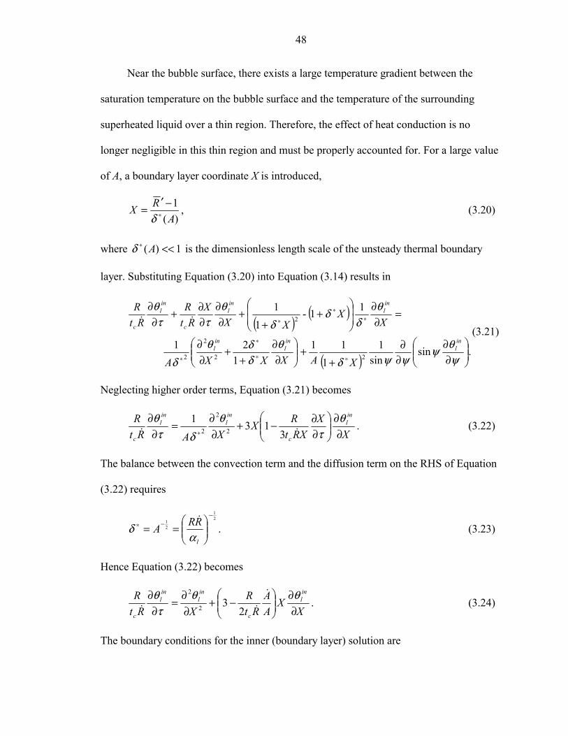
48
Near the bubble surface, there exists a large temperature gradient between the
saturation temperature on the bubble surface and the temperature of the surrounding
superheated liquid over a thin region. Therefore, the effect of heat conduction is no
longer negligible in this thin region and must be properly accounted for. For a large value
of A, a boundary layer coordinate X is introduced,
)(1
ARX ∗
−′=δ
, (3.20)
where 1)( <<∗ Aδ is the dimensionless length scale of the unsteady thermal boundary
layer. Substituting Equation (3.20) into Equation (3.14) results in
( ) ( )
( ) .sinsin
11
111
21
11-1
1
22
2
2
2
∂∂
∂∂
++
∂∂
++
∂∂
=∂∂
+
++
∂∂
∂∂+
∂∂
∗∗
∗
∗
∗∗
∗
ψθψ
ψψδθ
δδθ
δ
θδ
δδ
θττ
θ
inl
inl
inl
inl
inl
c
inl
c
XAXXXA
XX
XXX
RtR
RtR
DD
(3.21)
Neglecting higher order terms, Equation (3.21) becomes
XX
XRtRX
XARtR in
l
c
inl
inl
c ∂∂
∂∂−+
∂∂
=∂∂
∗
θτ
θδτ
θDD 3
1312
2
2 . (3.22)
The balance between the convection term and the diffusion term on the RHS of Equation
(3.22) requires
21
21
−−∗
==
l
RRAα
δD
. (3.23)
Hence Equation (3.22) becomes
XX
AA
RtR
XRtR in
l
c
inl
inl
c ∂∂
−+
∂∂
=∂∂ θθτθ D
DD 232
2
. (3.24)
The boundary conditions for the inner (boundary layer) solution are

49
0=−−
== XatTTTT
bw
bsatsat
inl θθ , (3.25)
∞→= Xatinl 1θ . (3.26)
For 1<<τ , 21
)( ttR ∝ and τ≈Rt
R
cD
. Thus, the LHS of Equation (3.24) is small and can
also be neglected. Equation (3.24) then reduces to
032
2
=∂∂
+∂∂
XX
X
inl
inl θθ
for 1<<τ . (3.27)
The solution for Equation (3.27) is
( ) satsatinl Xerf θθθ +−= 2
3)1( . (3.28)
For 1<<τ , by matching the outer and inner solutions given by Equation (3.19) and
Equation (3.28), the uniformly valid asymptotic solution of the bulk liquid temperature
for the saturated boiling problem considered here is obtained,
( ) ( ) ( )XerfcRRRRf satl 2
3
313
30
30 111
cos−+
−′+= θ
δψθ , (3.29)
where bw
bsatsat TT
TT−−
=θ and erfc is the complimentary error function. Equation (3.29) is an
asymptotic solution for lθ valid for 1<<τ .
The asymptotic solution given by Equation (3.29) for the liquid thermal field
provides an analytical framework to understand: 1) how the temperature field of
background superheated bulk liquid boundary layer influences the temperature lθ near
the vapor bubble through the function f; 2) how the bubble growth R(t) and liquid thermal
diffusivity affect the liquid thermal field lθ through the rescaled inner variable X as

50
defined in Equation (3.20) and Equation (3.23); and 3) how the folding of the temperature
contours near the bubble occurs through the dependence of ψcos term in Equation
(3.29). More importantly, from a computational standpoint, it provides: 1) an accurate
measure on the thickness of the rapidly moving thermal boundary layer; and 2) a reliable
guideline for estimating the adequacy of computational resolution in order to obtain an
accurate assessment of heat transfer to the bubble.
3.2.5 Initial Conditions
The computation must start from a very small but nonzero initial time 0τ , so that
)( 0τR is sufficiently small at the initial stage. To obtain enough temporal resolution for
the initial rapid growth stage and to save computational effort for the later stage, the
following transformation is used,
2στ = . (3.30)
Thus a constant “time step” σ∆ can be used in the computation.
The initial temperature profile inside the superheated bulk liquid thermal boundary
layer plays an important role to the solution of lθ , which in turn affects the heat transfer
to the bubble through the dome.
There exist both experimental and theoretical studies that have considered the bulk
liquid temperature profile in the vicinity of a vapor bubble. Hsu (1962) estimated the
temperature profile of the superheated thermal layer adjacent to the heater surface and
found the layer to be quite thin; thus the temperature gradient inside the thermal layer is
almost linear. However, beyond the superheated layer the temperature is held essentially
constant at the bulk temperature due to strong turbulent convection. The experimental
study by Wiebe and Judd (1971) revealed similar results. It was found that the

51
superheated bulk liquid thermal boundary layer thickness, δ, decreases with increasing
wall heat flux due to enhanced turbulent convection. A high wall heat flux results in
increased bubble generation, and the bulk liquid is stirred more rapidly by growing and
departing vapor bubbles. To estimate the superheated layer thickness, Hsu (1962) used a
thermal diffusion model within the bulk liquid. Han and Griffith (1965) used a similar
model and estimated the thickness to be
wl tπαδ = , (3.31)
where tw is the waiting period. The thermal diffusion model often overestimates the
thermal layer thickness, as it neglects the turbulent convection, which is quite strong as
reported by Hsu (1962) and Wiebe and Judd (1971).
Generally, the bulk liquid temperature profile is almost linear inside the
superheated thermal boundary layer, and remains essentially uniform at the bulk
temperature bT beyond the superheated background thermal boundary layer.
Accordingly, the initial condition for the bulk liquid thermal field used in the numerical
solution is given by
≥
<−=
δ
δδθ
z
zz
,0
,10 . (3.32)
In the asymptotic solution, the discontinuity of zl ∂∂θ in the above profile causes
the solution for lθ to be discontinuous. For clarity, the following exponential profile is
employed in representing the asymptotic solution
−=δ
θ zexp0 . (3.33)

52
3.2.6 Solution Procedure
An Euler backward scheme is used to solve Equation (3.14). A second order
upwind scheme is used for the convection term and a central difference scheme is used
for the thermal diffusion terms.
After the bulk liquid temperature field is obtained, the solid heater temperature
field is solved, and the bubble radius )(τR is updated using Equation (3.3) and Euler’s
explicit scheme. The information for )(τR is a necessary input in Equation (3.14).
Although the solution for )(τR is only first order accurate in time, the )( τ∆O accuracy is
not a concern here because a very small τ∆ has to be used to ensure sufficient resolution
during the early stages. Typically, 410=n time steps are used.
3.3 Results and Discussions
3.3.1 Asymptotic Structure of Liquid Thermal Field
To gain an analytical understanding of the liquid thermal field near the bubble and
to validate the accuracy of the computational treatment for the thin unsteady thermal
boundary layer, comparison between the computational and the asymptotic solutions for
lθ near the bubble surface is first presented. As mentioned previously, the validity of the
outer solution of the asymptotic analysis only requires 1>>A , which is satisfied under
most conditions due to rapid vapor bubble growth. The inner solution is valid for 1<<τ
in addition to 1>>A .
The comparison is presented for bubble growth in saturated liquid with A=14000.
The initial temperature profile follows Equation (3.33) and 5.0=cRδ , in which cR is the
bubble radius at ct . There are 200 and 50 grid intervals along the R′ - and ψ -directions,

53
respectively. The grid stretching factors are 65.0=′RS and 73.0=ψS for the
computational case.
Figure 3-4 compares the temperature profiles between the asymptotic and
numerical solutions at 001.0=τ , 0.01, 0.1, and 0.3 for �0=ψ , 40°, and 71°. There are
two important points to be noted. First of all, it is seen that the temperature gradient is
indeed very large near the bubble surface because the unsteady thermal boundary layer is
very thin. Secondly, numerical solutions agree very well with the asymptotic solutions at
001.0=τ and 0.01. The excellent agreement between the numerical and analytical
solutions indicates that the numerical treatment in this study is correct. At 1.0=τ and
0.3, the asymptotic inner solution given by Equation (3.29) is no longer accurate, while
the outer solution remains valid because 1>>A is the only requirement. At 1.0=τ and
0.3 the numerical solution matches very well with the outer solution. This again
demonstrates the integrity of the present numerical solution over the entire domain due to
sufficient computational resolution near the bubble surface and removal of undesirable
numerical diffusion through the use of second order upwind scheme in the radial
direction for Equation (3.14).
The large temperature gradient near the dome causes high heat transfer from the
superheated liquid to the vapor bubble through the dome. This large gradient results from
the strong convection effect that is caused by the rapid bubble growth (see Equation
(3.14) for the origin in the governing equation and Equation (3.19) for the explicit
dependence on the bubble growth). Thus the bulk liquid in the superheated boundary
layer supplies a sufficient amount of energy to the bubble.

54
Figure 3-4. Comparison of the asymptotic and the numerical solutions at τ =0.001, 0.01, 0.1 and 0.3 for ψ=0°, 40°, and 71°.
To capture the dynamics of the unsteady boundary layer, a sufficient number of
computational grids is required inside this layer. The asymptotic analysis gives an
estimate for the unsteady boundary layer thickness on the order of
025.014000
3~ =∗δ , which agrees with the numerical solution in Figure 3-4. At
01.0=τ in Figure 3-4, the discrete numerical results are presented. There are about 23
points inside the layer of thickness 025.0=∗δ . This provides sufficient resolution for the
R' -1
θ l
10-3 10-2 10-1 100 1010
0.1
0.2
0.3
0.4
0.5
0.6
0.7
0.8
0.9
1
ψ=0o (Numerical)ψ=40o (Numerical)ψ=71o (Numerical)ψ=0o (Asymptotic)ψ=40o (Asymptotic)ψ=71o (Asymptotic)
τ=0.1
_R' -1
θ l
10-3 10-2 10-1 100 1010
0.1
0.2
0.3
0.4
0.5
0.6
0.7
0.8
0.9
1
ψ=0o (Numerical)ψ=40o (Numerical)ψ=71o (Numerical)ψ=0o (Asymptotic)ψ=40o (Asymptotic)ψ=71o (Asymptotic)
τ=0.3
_
R' -1
θ l
10-3 10-2 10-1 100 1010
0.1
0.2
0.3
0.4
0.5
0.6
0.7
0.8
0.9
1
ψ=0o (Numerical)ψ=40o (Numerical)ψ=71o (Numerical)ψ=0o (Asymptotic)ψ=40o (Asymptotic)ψ=71o (Asymptotic)
τ=0.001
_R' -1
θ l
10-3 10-2 10-1 100 1010
0.1
0.2
0.3
0.4
0.5
0.6
0.7
0.8
0.9
1
ψ=0o (Numerical)ψ=0o (Asymptotic)ψ=40o (Numerical)ψ=40o (Asymptotic)ψ=71o (Numerical)ψ=71o (Asymptotic)
τ=0.01
_

55
temperature profile in the unsteady thermal boundary layer. In contrast, most
computational studies on the thermal field around the bubble dome reported in the open
literature have insufficient grid resolution adjacent the dome, which leads to an
inaccurate heat transfer assessment.
Figure 3-5 shows the effect of parameter A on the asymptotic solution. When A is
large, the asymptotic and numerical solutions agree very well. The discrepancy between
asymptotic and numerical solutions inside the unsteady thermal boundary layer increases
when A decreases. However, the outer solution remains valid for the far field even when
A becomes small.
R'-1
θ l
10-3 10-2 10-1 100 101-0.1
0
0.1
0.2
0.3
0.4
0.5
0.6
0.7
0.8
0.9
1
_
τ=0.01ψ=40o
100001000
10010
A=14000
Asymptotic
Numerical
Figure 3-5. Effect of parameter A on the liquid temperature profile near bubble.
The temperature contours shown in Figure 3-6 are difficult to obtain
experimentally. Only recent progress in holographic thermography permits such
measurements. Ellion (1954) has stated that there exists an unsteady thermal boundary

56
layer contiguous to the vapor bubble during the bubble growth. Recently, Mayinger
(1996) used a holography technique to capture the folding of the temperature contours
during subcooled nucleate boiling. Although his study considered subcooled nucleate
boiling, the pattern of the temperature distribution near the bubble dome by Mayinger
(1996) is very similar to that shown in the Figure 3-6. It is expected that experimental
evidence of contour folding in saturated nucleate boiling will be reported in the future.
3.3.2 Constant Heater Temperature Bubble Growth in the Experiment of Yaddanapudi and Kim
In the experiment of Yaddanapudi and Kim (2001), single bubbles growing on a
heater array kept at nominally constant temperature were studied. The liquid used is
FC-72, and the wall superheat is maintained at 22.5 °C, so that Jacob number is 39. The
bubble shape in the early stage appears to be hemispherical. To calculate the heat flux
from the microlayer to the vapor bubble in the present model, the microlayer wedge angle
φ or constant 1c in Equation (3.4) must be determined. Neither φ or 1c has been
measured. However, the authors have reported the amount of wall heat flux from the wall
to the bubble through an equivalent bubble diameter eqd assuming that the wall heat flux
is the only source of heat entering the bubble. Since in the present model this heat flux is
assumed to pass through the microlayer, it may be used to evaluate the constant 1c via
trial and error. The superheated thermal boundary layer thickness δ of the bulk liquid in
Equation (3.32) is also a required input. The computed growth rate )(tR is matched with
the experimentally measured )(tR in order to determine δ. The simulation is carried out
only for the early stage of bubble growth. This is because after t=6-8×10⁻⁴s the base of
the bubble does not expand anymore, and the bubble shape deviates from a hemisphere.

57
Furthermore, there is the possibility of the microlayer being dried out in the latter growth
stages as a result of maintaining a constant wall temperature, as was observed by Chen et
al. (2003).
Figure 3-6. The computed isotherms near a growing bubble in saturated liquid at τ=0.01,
τ=0.1,τ=0.3, and τ=0.9.
Figure 3-7 shows the computed equivalent bubble diameter )(tdeq , together with
the experimentally determined equivalent )(tdeq . In the present model, eqd is calculated
using
mrLz
mll
bfgv dA
nTk
dtdVh
)(=∫ ∂
∂−=⋅ρ , (3.34)
0.9
0.88
0.85
0.8
0.77
0.75
0.7
0.98
0.96
0.94
0.92
R' -10 0.5 1 1.5 2
0
0.5
1
1.5
2
_
τ=0.01
0.9
0.8
0.75
0.65
0.6
0.55
0.5
0.45
0.4
0.35
R' -10 0.5 1 1.5 2
0
0.5
1
1.5
2
_
τ=0.1
0.7
0.6
0.5
0.4
0.3
0.25
0.2
0.95
0.9
0.85
0.8
0.75
0.65
0.15
R'-10 0.5 1 1.5 2
0
0.5
1
1.5
2
_
τ=0.30.4
0.3
0.2
0.15
0.9
0.8
0.7
0.6
0.5
0.1
0.05
R'-10 0.5 1 1.5 2
0
0.5
1
1.5
2
_
τ=0.9

58
where 3
6 eqb dV π= . The heat flux includes only that from the microlayer and this allows
1c to be evaluated. For eqd , to match the measured data as shown in Figure 3-7, it
requires 1c =3.0.
t (s)
d(t)
(m)
0 0.0002 0.0004 0.0006 0.00080
5E-05
0.0001
0.00015
0.0002
0.00025
0.0003
0.00035
0.0004
0.00045
0.0005
deq(t) present modeldeq(t) measurement
Figure 3-7. Comparison of the equivalent bubble diameter eqd for the experimental data
of Yaddanapudi and Kim (2001) and that computed for heat transfer through the microlayer ( 1c =3.0).
Figure 3-8 compares the computed bubble diameter )(2)( tRtd = and those
reported by Yaddanapudi and Kim (2001). In Figure 3-8, δ=30µm is used in addition to
1c =3.0 in matching the predicted bubble growth with measured data. The good
agreement obtained can be partly attributed to the adjustment in the superheated bulk
liquid thermal boundary layer thickness δ. Because the heat transfer to the bubble
(through the microlayer and through the dome) is of two different mechanisms, the good

59
agreement over the range is an indication of the correct physical representation by the
present model.
Figure 3-9 shows the total heat entering bubble and the respective contribution
from the microlayer and from the unsteady thermal boundary layer. The contribution
from the unsteady thermal boundary layer accounts for about 70% of the total heat
transfer. It was reported by Yaddanapudi and Kim (2001) that approximately 54% of the
total heat is supplied by the microlayer over the entire growth cycle. Since, the simulation
is only carried out for the early stage of bubble growth, it is difficult to compare the
microlayer contribution to heat transfer reported by Yaddanapudi and Kim (2001) with
that predicted by current model. At the end, the bubble expands outside the superheated
boundary layer and protrudes into the saturated bulk liquid. The heat transfer from dome
thus slows down. Hence, the 54% for the entire bubble growth period dose not contradict
a higher percentage of contribution computed from the unsteady thermal boundary layer
during the early stages.
Figure 3-10 shows the computed temperature contours associated with
Yaddanapudi and Kim’s (2001) experiment for the estimated δ and 1c . Folding of the
temperature contours is clearly observed in the simulation for saturated boiling.
3.3.3 Effect of Bulk Liquid Thermal Boundary Layer Thickness on Bubble Growth
Since the superheated bulk liquid thermal boundary layer thickness, δ, determines
how much heat is stored in the layer, it is instructive to conduct a parametric study on the
effects bubble growth with varying δ. All parameters are the same as those used in
Yaddanapudi and Kim’s (2001) experiment except that δ is varied. Hence the influence
of the superheated thermal boundary layer thickness δ on the bubble growth is elucidated.

60
t (s)
d(t)
(m)
0 0.0002 0.0004 0.0006 0.00080
5E-05
0.0001
0.00015
0.0002
0.00025
0.0003
0.00035
0.0004
0.00045
0.0005
d(t) present modeld(t) measurement
Figure 3-8. Comparison of bubble diameter, d(t), between that computed using the present model and the measured data of Yaddanapudi and Kim (2001). Here,
1c =3.0 and δ=30µm.
t(s)
heat
(J)
0 0.0002 0.0004 0.0006 0.00080
2E-06
4E-06
6E-06
8E-06
1E-05
1.2E-05
1.4E-05
1.6E-05
total heat entering the bubbleheat from micorlayerheat from bulk liquid thermal boudary layer
Figure 3-9. Comparison between heat transfer to the bubble through the vapor dome and
that through the microlayer.

61
Figure 3-11 shows the effect on the bubble growth rate of varying δ (from 1µm to
100µm). The thicker the bulk liquid thermal boundary layer, the faster the bubble grows.
A large δ implies a larger amount of heat is stored in the background bulk liquid
surrounding the bubble. It is also clear that when δ approaches zero, the bubble growth
rate becomes unaffected by the variation of δ. The reason is when δ is small, most of heat
supplied for bubble growth comes from the microlayer and the contribution from the
dome can be neglected.
Figure 3-10. The computed isotherms in the bulk liquid corresponding to the thermal
conditions reported by Yaddanapudi and Kim (2001).
0.005
0.050.10.30.50.7
0.9
R' -10 0.5 1 1.5 2
0
0.5
1
1.5
2
_
t=0.96ms
0.005
0.050.10.30.50.70.9
R' -10 0.5 1 1.5 2
0
0.5
1
1.5
2
_
t=0.36ms
0.005
0.050.1
0.3
0.5
0.7
0.9
R' -10 0.5 1 1.5 2
0
0.5
1
1.5
2
_
t=0.12ms
0.05
0.1
0.2
0.3
0.4
0.5
0.6
0.7
0.8
0.9
R' -10 0.5 1 1.5 2
0
0.5
1
1.5
2
_
t=0.0012ms

62
It is also noted that for δ=100µm, if the bubble eventually grows to about several
millimeters, the effect of the bulk liquid thermal boundary layer is negligible on )(tR for
most of the growth period except at the very early stages. Physically, this is because the
bubble dome is quickly exposed to the saturated bulk liquid so that it is at thermal
equilibrium with the surroundings. For small bubbles, it will be immersed inside the
thermal boundary layer most of time. Hence the effect of the bulk liquid thermal
boundary layer becomes significant for the bubble growth.
t(s)
d(m
)
0 0.0002 0.0004 0.0006 0.0008 0.0010
0.0001
0.0002
0.0003
0.0004
0.0005
0.0006
0.0007
δ=100 µm
δ=50 µm
δ=30 µm
δ=10 µm
δ=5 µmδ=1 µm
Figure 3-11. Effect of bulk liquid thermal boundary layer thickness δ on bubble growth.
The microlayer angle φ and the superheated bulk liquid thermal liquid boundary
layer thickness δ are the required inputs to compute bubble growth in the present model.
However, neither of these parameters is typically measured or reported in bubble growth
experiments. It is strongly suggested that the bulk liquid thermal boundary layer

63
thickness δ be measured and reported in future experimental studies. For a single bubble
study, δ in the immediate neighborhood of the nucleation site should be measured.
3.4 Conclusions
In this study, a physical model is presented to predict the early stage bubble growth
in saturated heterogeneous nucleate boiling. The thermal interaction of the temperature
fields around the growing bubble and vapor bubble together with the microlayer heat
transfer is properly considered. The structure of the thin unsteady liquid thermal
boundary layer is revealed by the asymptotic and numerical solutions. The existence of a
thin unsteady thermal boundary layer near the rapidly growing bubble allows for a
significant amount of heat flux from the bulk liquid to the vapor bubble dome, which in
some cases can be larger than the heat transfer from the microlayer. The experimental
observation by Yaddanapudi and Kim (2001) on the insufficiency of heat transfer to the
bubble through the microlayer is elucidated. For thick superheated thermal boundary
layers in the bulk liquid, the heat transfer though the vapor bubble dome can contribute
substantially to the vapor bubble growth.

64
CHAPTER 4 ANALYSIS ON COMPUTATIONAL INSTABILITY IN SOLVING TWO-FLUID
MODEL
The two-fluid model is widely used in studying gas-liquid flow inside pipelines
because it can qualitatively predict the flow field with a low computational cost.
However, the two-fluid model becomes ill-posed when the slip velocity between the gas
and the liquid exceeds a critical value. Computationally, even before the flow becomes
unstable, computations can be quite unstable to render the numerical result unreliable. In
this study computational stability of various convection schemes for the two-fluid model
is analyzed. A pressure correction algorithm is carefully implemented to minimize its
effect on stability. Von Neumann stability analysis for the wave growth rates by using the
1st order upwind, 2nd order upwind, QUICK (quadratic upstream interpolation for
convection kinematics), and the central difference schemes are conducted. For inviscid
two-fluid model, the central difference scheme is more accurate and more stable than
other schemes. The 2nd order upwind scheme is much more susceptible to instability for
long waves than the 1st order upwind and inaccurate for short waves. The instability
associated with ill-posedness of the two-fluid model is significantly different from the
instability of the discretized two-fluid models. Excellent agreement is obtained between
the computed and predicted wave growth rates, when various convection schemes are
implemented.
The pressure correction algorithm for inviscid two-fluid model is further extended
to the viscous two-fluid model. For a viscous two-fluid model, the diffusive viscous

65
effect is modeled as a body force resulting from the wall friction. Von Neumann stability
analysis is carried out to assess the performances of different discretization schemes for
the viscous two-fluid model. The central difference scheme performs best among the
schemes tested. Despite its nominal 2nd order accuracy, the 2nd order upwind scheme is
much more inaccurate than the 1st order upwind scheme for solving viscous two-fluid
model. Numerical instability is largely the property of the discretized viscous two-fluid
model but is strongly influenced by VKH instability. Excellent agreement between the
computed results and the predictions from von Neumann stability analysis for different
numerical scheme is obtained. Inlet disturbance growth test shows that the pressure
correction scheme is capable to correctly handle the viscous two-phase flow in a pipe.
4.1 Inviscid Two-Fluid Model
4.1.1 Introduction
Gas-liquid flow inside a pipeline is prevalent in the handling and transportation of
fluids. A reliable flow model is essential to the prediction of the flow field inside the
pipeline. To fully simulate the system, Navier–Stokes equations in three-dimensions are
required. However, it is very expensive to simulate complex two-phase flows in a long
pipe with today’s computer capability. To reduce the computational cost and obtain basic
and essential flow properties of industrial interest, such as gas volume fraction, liquid and
gas velocity, pressure, a one-dimensional model is necessary. The two-fluid model is
considered to give a realistic prediction for the gas-liquid flow inside a pipeline.
The two-fluid model (Wallis, 1969; Ishii, 1975), also known as the separated flow
model, consists of two sets of conservation equations for mass, momentum and energy
for the gas phase and the liquid phase. Although it has success in simulating two-phase
flow in a pipeline, the two-fluid model suffers from an ill-posedness problem. When the

66
slip velocity between liquid and gas exceeds a critical value that depends on gravity and
liquid depth, among other flow properties, the governing equations do not possess real
characteristics (Gidaspow, 1974; Jones and Prosperettii, 1985; Song and Ishii, 2000).
This ill-posedness condition suggests that the results of the two-fluid model under such
condition do not reflect the real flow situation in the pipe. The two-fluid model only gives
meaningful results when the relative velocity between the gas and liquid phase is below
the critical value. However, this critical value coincides with the stability condition of
inviscid Kelvin-Helmholtz instability (IKH) analysis (Issa and Kempf, 2002). Because
the IKH instability results in the flow regime transition from the stratified flow to the slug
flow or annular flow (Barnea and Taitel, 1994a), ill-posedness of two-fluid model has
been interpreted as to trigger the flow regime transition (Brauner and Maron, 1992;
Barnea and Taitel, 1994a).
The computational methods for solving the two-fluid model have been investigated
by many researchers. For computational simplicity, it is further assumed that both liquid
and gas phases are incompressible. This is valid because most stratified flows are at
relatively low speed compared with the speed of sound. To solve the incompressible
two-fluid equations, one approach is to simplify the governing system to only two
equations for liquid volume fraction and liquid velocity and neglect the transient terms in
the gas mass and momentum equations (Chan and Banerjee, 1981; Barnea and Taitel,
1994b). A more effective method is to use a pressure correction scheme (Patanka 1980).
Issa and Woodburn (1998), and Issa and Kempf (2003) applied the pressure correction
scheme for the two-fluid model and simulated the stratified flow and the slug flow inside
a pipe.

67
When two-fluid model becomes ill-posed, the solution becomes unstable. A good
discretized model should be capable of capturing the incipience of the instability point.
However, numerical instability may not be the same as the instability caused by the
ill-posedness. Lyczkowski et al. (1978) used von Neumann stability analysis to study a
compressible two-fluid model with their numerical scheme and found that numerical
instability and ill-posedness may not be identical. However, their two-fluid model lacked
the gravitational term and the study focused on one specific discretization scheme and is
thus incomplete. Stewart (1979), Ohkawa and Tomiyama (1995) attempted to analyze the
numerical stability of an incompressible two-fluid model with a simplified model
equation as an alternative. Their study showed that higher order upwind schemes yield a
more unstable numerical solution than the 1st order upwind scheme.
In this study, a pressure correction scheme is employed to solve the two-fluid
model. It is designed to increase the computational stability when the flow is near the
ill-posedness condition. The von Neumann stability analysis is carried out to study the
stability of the discretized two-fluid model with different interpolation schemes for the
convection term. For the wave growth rates using the 1st order upwind, 2nd order upwind,
QUICK, and central difference schemes, the central difference scheme is more accurate
and more stable. Excellent agreement for the wave growth rates is obtained between the
analysis and the actual computation under various configurations.
4.1.2 Governing Equations
The basis of the two-fluid model is a set of one-dimensional conservation equations
for the balance of mass, momentum and energy for each phase. The one-dimensional
conservation equations are obtained by integrating the flow properties over the
cross-sectional area of the flow, as shown in Figure 4-1.

68
Liquid phase
Gas phase
Interface
Liquid velocity lu
Gas velocity gu
Gravity g
Gas velome faction gα
Liquid velome faction lα
Pipe cross section
gh
lh
Figure 4-1. Schematic of two-fluid model for pipe flow.
Because the ill-posedness originates from the hydrodynamic instability of the
two-fluid model, only continuity and momentum equations are considered in the inviscid
two-fluid model. Furthermore, no mass and energy transfer occurs between two phases.
Surface tension is also neglected since it only acts on small scales, while the waves
determining the flow structure in pipe flows are usually of long wavelength. The gas
phase is assumed to be incompressible, as the Mach number of the gas phase is usually
very low for the stratified flow. Hence, the mass conservation equations for liquid phase
is
( ) ( ) 0=∂∂+
∂∂
lll uxt
αα , (4.1)
where lα is liquid volume fraction, lρ is liquid density, lu is the liquid velocity, t is the
time, x is the axial coordinate.
The liquid layer momentum conservation equation is
( ) ( ) βααβρααα sincos2 g
xHg
xpu
xu
t ll
li
l
lllll −
∂∂−
∂∂−=
∂∂+
∂∂ , (4.2)

69
where ip is the pressure at the liquid-gas interface, g is gravitational accelerator, β is the
angle of inclination of the pipe axis from the horizontal lane, and lH is the liquid phase
hydraulic depth. It is defined as
l
l
ll
ll h
Hαα
αα
′=
∂∂= , (4.3)
where lh is the liquid layer depth. The second term on the right hand side of Equation
(4.2) represents the effect of gravity on the wavy surface of liquid layer.
The gas phase mass conservation equation is
( ) ( ) 0=∂∂+
∂∂
ggg uxt
αα , (4.4)
where gρ , gα , gu are density , volume fraction, and velocity of gas phase. It is noted that
1=+ gl αα . (4.5)
The momentum equation for gas phase is
( ) ( ) βααβρα
αα sincos2 gx
Hgxpu
xu
t gl
gi
g
ggggg −
∂∂−
∂∂−=
∂∂+
∂∂ , (4.6)
where gH is the gas phase hydraulic depth. It is defined as
g
g
gg
gg h
Hαα
αα
′=
∂∂= , (4.7)
where gh is the gas layer depth,
4.1.3 Theoretical Analysis
4.1.3.1 Characteristic analysis and ill-posedness
It is well known that the initial and boundary conditions need to be imposed
consistently for a given system of differential equations. The condition is well-posed if

70
the solution depends in a continuous manner on the initial and boundary conditions. That
is, a small perturbation of the boundary conditions should give rise to only a small
variation of the solution at any point of the domain at finite distance from the boundaries
(Hirsch, 1988).
Equations (4.1, 4.2, 4.4 and 4.6) form a system of 1st order PDEs, for which the
characteristic roots, λ, of the system can be found. If λ’s are real, the system is
hyperbolic. Complex roots imply an elliptic system, which causes the two-fluid model
system to become ill-posed because only initial conditions can be specified in the
temporal direction. Any infinitesimal disturbance will cause the waves to grow
exponentially without bound when λ’s are complex valued.
Let U be the vector Tgll puu ),,,(α . Equations (4.1, 4.2, 4.4 and 4.6) can be written
in vector form as
][][][ Cx
Bt
A =∂∂+
∂∂ UU , (4.8)
where [A], [B] and [C] are coefficient matrices, given by
−
−=
000000010001
][
gg
ll
uu
A
αα
, (4.9a)
+−
+
−
=
g
ggggg
l
lllll
gg
ll
ugHu
ugHu
uu
B
ρα
αβ
ρααβ
αα
20cos
02cos
0000
][
2
2 , (4.9b)

71
[ ]
−−
=
βαβα
sinsin
00
gg
C
g
l. (4.9c)
The characteristic roots of the system is determined by solving λ from the
following
0][][ =− BA λ . (4.10)
where • denotes the determinant of the matrix. Substituting Equations (4.9a) and (4.9b)
into Equation (4.10) results in
0
)2(0cos)(
0)2(cos)(
00)(00
=
−−−−−
−−−−
−−−−−
g
gggggg
l
llllll
gg
ll
ugHuu
ugHuu
uu
ρα
λαβλ
ραλαβλ
αλαλ
. (4.11)
After expansion of the above determinant, the characteristic polynomial for λ is
obtained:
( ) ( ) ( ) 0cos122 =′
−−−+− βα
ρρλαρλ
αρ
guul
glll
lg
g
g . (4.12)
The roots are
( )
g
g
l
l
lggl
gl
l
gl
g
gg
l
ll uuguu
αρ
αρ
ααρρ
βαρρ
ραρ
αρ
λ+
−−′
−±
+
=
2sin
. (4.13)

72
When 0=g , Equation (4.13) can have real roots only if lg uu ==λ . Otherwise, the
two-fluid model is ill-posed (Gidaspow, 1974). If 0≠g , the well-posedness with real
roots requires
( ) βαρρ
ρα
ρα
sin222 gUuuUl
gl
g
g
l
lclg ′
−
+=∆<−=∆ . (4.14)
Equation (4.14) gives the critical value cU∆ for the slip velocity U∆ between two
phases beyond which the system becomes ill-posed. The two-fluid model stability
criterion from the characteristic analysis is exactly the same as that from the IKH analysis
on two-fluid model by Barnea and Taitel (1994) as shown below.
4.1.3.2 Inviscid Kelvin-Helmholtz (IKH) analysis and linear instability
IKH analysis (Barnea and Taitel, 1994) provides a stability condition for the
linearized two-fluid model as well as useful information on the growth rate of an
infinitesimal disturbance in the two-fluid model.
Splitting the flow variables into the base variables and the small disturbances, such
as ll αα ~+ , expressing the disturbances on the form of
( )( )kxtIl −= ωεα exp~ , (4.15a)
( )( )kxtIu ll −= ωε exp~ , (4.15b)
( )( )kxtIu gg −= ωε exp~ , (4.15c)
( )( )kxtIp p −= ωε exp~ , (4.15d)
where “~” denote disturbance value, 1−=I denotes imaginary unit, ε is the amplitude
of perturbation, ω is the angular frequency of wave and k is the wavenumber.
Substituting them into the differential governing equations (4.1, 4.2, 4.4 and 4.6), and

73
linearizing the resulting equations, the following system is obtained for the disturbance
amplitudes, ( )Tpgl εεεε ,,,
0
0cos
0cos
0000
=
−−
−−
−−−
p
g
l
gg
l
l
ll
l
l
gg
ll
kkugH
k
kkugHk
kkukku
εεεε
ρωβ
α
ρωβ
α
αωαω
. (4.16)
For non-trivial solutions to exist, the following dispersion relation between the wave
speed c and the angular frequency ω must hold
( )
g
g
l
l
lggl
gl
l
gl
g
gg
l
ll uuguu
kc
αρ
αρ
ααρρ
θαρρ
ραρ
αρ
ω
+
−−′
−±
+
==
2sin
. (4.17)
It is note that the negative imaginary part of ω determines the growth rate of disturbance.
Equation (4.17) is identical to Equation (4.13), only with λ being replaced by c. Details
of the derivation for IKH stability condition can be found in Barnea and Taitel (1994).
4.1.4 Analysis on Computational Instability
4.1.4.1 Description of numerical methods
In general, the governing equations (4.1, 4.2, 4.4, and 4.6) are solved iteratively.
The basic procedure is to solve the continuity equation of liquid for the liquid volume
fraction, and the liquid and gas phase momentum equations for the liquid and gas phase
velocities. To obtain a governing equation for the pressure, Equation (4.1) and Equation
(4.4) are first combined to form a total mass conservation,
( ) ( ) 0=∂∂+
∂∂
llgg ux
ux
αα . (4.18)

74
Substituting the liquid and gas momentum equations into the above leads to
( )
.sincossincos
222
2
∂∂
+∂∂
∂∂+
+∂∂=
∂∂
+
∂∂
βααββααβ
ααρα
ρα
gx
Hggx
Hgx
uuxx
px
gl
gll
l
ggllg
g
l
l
(4.19)
To solve the pressure equation, SIMPLE type of pressure correction scheme (Patanka,
1982; Issa and Kempf, 2002) is used in this study.
A finite volume method is employed to discretize governing equation. A staggered
grid (Figure 4-2) is adopted to obtain compact stencil for pressure (Peric and Ferziger,
1996). On the staggered grids, the fluid properties such as volume fractions, density and
pressure are located at the center of main control volume, and the liquid and gas
velocities are located at the cell face of main control volume. Figure 4-2 shows the
staggered grids arrangement.
Wu Pu Eu
Pp
Pαx
Velocity control volume
Main control volume
EpWp
Wα Eα
wu eu
wp ep
eαwα
Figure 4-2. Staggered grid arrangement in two-fluid model.
The Euler backward scheme is employed for the transient term. The discretized
liquid continuity equation becomes
( ) ( )( ) ( ) ( ) 00 =−+−∆∆
wllellPlPl uutx αααα , (4.20)

75
where the superscript 0 denotes the values of the last time step. The subscript P refers to
the center of the main control volume, and subscripts e and w refer to the east face and
west face of main control volume, respectively. The liquid velocity on the cell face is
known, and the volume fraction on the cell face can be evaluated using various
interpolation schemes. Among them, central difference (CDS), 1st order upwind (FOU),
2nd order upwind (SOU) and QUICK schemes are commonly used. Equation (4.4) for the
gas phase is similarly discretized.
The liquid momentum equation is integrated on the velocity control volume. Using
similar notations, one obtains
( ) ( )( ) ( ) ( ) ( ) ( )( ) ( ) ( ) ( )( ) ( ) βαβααρα
αααα
sincos
0
gxgHpp
uuuuuutx
Pllelwlewl
Pl
wllwlellelPllPll
∆−−+−
=−+−∆∆
, (4.21)
where P, e, w refer to the center, east face and west face of the velocity control volume,
respectively. The cell face flux is the liquid velocity, which is obtained by using central
difference, and the volume fraction and liquid velocity at the cell face, which are
transported variables, can be interpolated by using different schemes. It is important to
note that the interpolation method used for the Equation (4.21) must be exactly the same
as those for Equation (4.20). For example, if FOU is used in Equation (4.20), the cell face
flux on the east face of velocity control volume in Equation (4.11) is
( ) ( ) ( ) ( )( ) ( ) ( )( )0,0, elEllelPllelell uMAXuuMAXuuu −−= ααα . (4.22)
If CDS is used in Equation (4.20), the cell face flux on the east face in Equation (4.21) is
evaluated as
( ) ( ) ( ) ( ) ( )elEllPll
elell uuu
uu2αα
α+
= . (4.23)

76
Using similar discretization procedure, the gas phase momentum equation is
integrated:
( ) ( )( ) ( ) ( ) ( ) ( )( ) ( ) ( ) ( )( ) ( ) .sincos
0
βαβααρα
αααα
gxgHpp
uuuuuutx
Pggelwlewg
Pg
wggwgeggegPggPgg
∆−−+−
=−+−∆∆
(4.24)
For convenience, the discretized mass or momentum equations are written in a
general form
BAAA WwEepp =Φ+Φ+Φ , (4.25)
where Φ is the variable to be solved, A is the coefficient, B is the general source term.
For the pressure correction scheme, Equation (4.18) is integrated across the main
control volume. The discretized equation is
( ) ( ) ( ) ( ) 0=−+− wllellwggegg uuuu αααα . (4.26)
Because Equation (4.18) is obtained by combining Equation (4.1) and Equation
(4.4), the discretization scheme for Equation (4.26) should be exactly the same as those
for Equation (4.20) and the discretized equation of Equation (4.3). For instance, if CDS is
used in Equation (4.20), it must be used in the main control volume for Equation (4.26):
( ) ( ) ( ) ( ) ( ) ( )
( ) ( ) ( ) ( ) ( ) ( ).0
22
22
=+
−+
+
+−
+
WlPlwl
ElPlel
WgPg
wgEgPg
eg
uu
uu
αααα
αααα
(4.27)
The final discretized pressure equation is obtained by substituting these two
momentum equations, Equation (4.21) and Equation (4.24) into Equation (4.26). This
yields
bpapapa WwEepp =′+′+′ , (4.28)

77
( ) ( )( )
( ) ( )( )
elpl
lElpl
evpv
vEvpve AA
a
+−
+−=
ρααα
ρααα
22, (4.29a)
( ) ( )( )
( ) ( )( )
wlpl
lWlpl
wvpv
vWvpvw AA
a
+−
+−=
ρααα
ρααα
22, (4.29b)
wep aaa −−= , (4.29c)
( ) ( ) ( ) ( ) ( ) ( )( ) ( ) ( ) ( ) ( ) ( ) .
22
22
elElPl
wlWlPl
evEvPv
wvWvPv
uaa
uaa
uaa
uaa
b
∗∗
∗∗
+−
++
+−
+=
(4.29d)
where, p′ represents the pressure correction value, ∗u represents the imbalanced
velocity, and pA is from the corresponding discretized liquid or gas momentum equation,
Equation (4.15). The flow chart of the pressure correction scheme is shown in Figure 4-3.
Similarly, the pressure correction schemes with FOU, SOU, CDS, and QUICK can
be obtained.
Consistently handling the discretization is critical to the reduction of numerical
diffusion and dispersion. Barnea and Taitel (1994) showed that the viscosity of fluid can
dramatically degrade the stability of two-fluid model through viscous Kelvin-Helmholtz
stability analysis. Although the viscosity in two-fluid model appears as the body force
instead of 2nd order derivative terms in the modified governing equation, it is
hypothesized that the numerical diffusion and dispersion appearing as derivative in the
modified governing equations produce similar impact on the stability of two-fluid model.

78
Solve lα and gα using Equation (4.20)
Solve lu and gu using Equation (4.21, 4.24)
Solve p′ using Equation (4.28)
Update lu and gu
No
Initial conditions
End
Yes
tt ∆+
Boundary condition
If maxtt = ?No
Yes
If lu converges?
Figure 4-3. Flow chart of pressure correction scheme for two-fluid model.
4.1.4.2 Code validation— dam-break flow
The pressure correction scheme is first validated by computing the transient flow
due to dam-break flow (Figure 4-4). The liquid flow is assumed to be over a horizontal
flat surface and the flow is assumed to be one-dimensional. On the left side of the dam is
a body of stationary water in the reservoir with the flat surface of height H. On the right

79
side of dam is a dry river bottom surface. After the dam breaks suddenly, the water in the
reservoir flows to the downstream due to the gravitational force. If there are no friction
between the fluid and the wall and no viscosity inside the fluid and air pressure is a
constant, an analytical solution for the liquid velocity based on St Venant equation can be
found (Zoppou and Roberts, 2003). The result is shown in Table 2.1.
Dam
Dry river plate
Reservoir H
x
y
x=0
Figure 4-4. Schematic for dam-break flow model.
To solve dam-break flow, the pressure at interface, the vapor phase density and
velocity are set to zero. Second order upwind scheme as the cell face interpolation
scheme is implemented in the pressure correction scheme. Figure 4-5 compares water
depth between the present numerical solution and the analytical solution at t=50s. Two
solutions match very well except at the tail end of the liquid, where the numerical
solution is smooth due to a little numerical dissipation. Figure 4-6 compares liquid
velocities between the numerical and analytical solutions at t=50s. Again, these two
solutions match very well except at the leading and tail ends. The discrepancy at the
leading end is due to that the liquid layer is too thin and the numerical result is prone to
error.

80
Table 4-1. Analytical solution for dam-break flow (Zoppou and Roberts, 2003). x( position) u ( water velocity) h (water depth)
gHtx −≤ 0=u Hh =
gHtxgHt 2≤<−
+=txgHu
32
2
294
−=t
xgHg
h
gHtx 2≥ 0=u 0=h
Although only the dynamics of liquid phase is considered in the dam-break flow, it
is still a solid step for validating the coupling of the pressure and liquid flow (liquid
volume fraction and liquid velocity) in numerical scheme. When both the liquid and the
gas phase present in the flow, the instability in two-fluid model rises due to the
interaction of the liquid and the gas phase, when the slip velocity is large. Numerical
instability of pressure correction scheme emerges and destroys the numerical results
when the two-fluid model near ill-posedness. This numerical instability will be
investigated in the next section and the code will be validated using the theoretical results
of inviscid Kelvin-Helmholtz analysis (Barnea and Taitel, 1994).
z(m)
h(m
)
0 500 1000 1500 20000
1
2
3
4
5
6
7
8
9
10
NumericalAnalytical
t=50 sec
t=0 sec
Figure 4-5. Water depth at t=50 seconds after dam break.

81
z(m)
velo
city
(m/s
)
0 500 1000 1500 20000
2
4
6
8
10
12
14
16
18
20
NumericalAnalytical
t=50 sec
Figure 4-6. Water velocity at t=50 seconds after dam break.
4.1.4.3 Von Neumann stability analysis for various convection schemes
Similar to the well-posedness of the differential equations, numerical stability is
essential to solve the discretized systems. Von Neumann stability analysis is commonly
used to analyze the stability of finite difference schemes (Hirsch, 1988; Shyy, 1994).
ui-1 ui-0.5 ui+0.5
pi-1 pi pi+0.5
αi+0.5αi-1 αi
x
Figure 4-7. Grid index number in staggered grid for von Neumann stability analysis.

82
To begin with, the 1st order upwind (FOU) scheme is used as an illustrative
example. For simplicity and for practical purpose, both liquid and gas velocities are
assumed positive. Discretization of Equation (4.20) with FOU scheme leads to
( ) ( ) ( ) ( ) ( ) ( )( ) 01
1
21
21 =−+∆
∆−
−−+
−nil
nil
nil
nil
nil
nil uux
tαα
αα. (4.30)
Splitting the variables into base value and disturbances, the linearized equation for
the disturbance lα is
( ) ( ) ( ) ( )( ) ( ) ( )( )( ) 0ˆˆˆˆˆˆ
1
1
21
21 =−−−+∆
∆−
−−+
−nil
nill
nil
nill
nil
nil uuux
tααα
αα, (4.31)
where “^” denotes disturbance values. The disturbances may be expressed as
( ) Ikxnnil eEεα =ˆ , (4.32a)
( ) Ikxnl
nil eEu ε=ˆ , (4.32b)
( ) Ikxnv
niv eEu ε=ˆ , (4.32c)
where E is a common amplitude factor, and k is the wavenumber. Equation (4.31) is
simplified to
( ) ( ) ( ) 011 21
211 =−+
−+−∆∆ −−− φφφ αεε II
llI
l eeeuGtx , (4.33)
where G is the amplification factor defined as
1−= n
n
EEG , (4.34)
and φ is phase angle:
xk ∆⋅=φ (4.35)
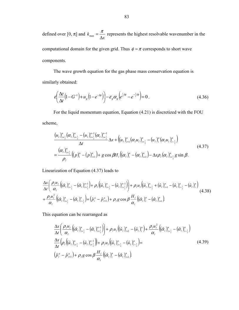
83
defined over [0, π] and x
k∆
= πmax represents the highest resolvable wavenumber in the
computational domain for the given grid. Thus πφ ≈ corresponds to short wave
components.
The wave growth equation for the gas phase mass conservation equation is
similarly obtained:
( ) ( ) ( ) 011 21
211 =−−
−+−∆∆ −−− φφφ αεε II
ggI
g eeeuGtz
. (4.36)
For the liquid momentum equation, Equation (4.21) is discretized with the FOU
scheme,
( ) ( ) ( ) ( )( ) ( ) ( ) ( )( )
( )( ) ( )( ) ( ) ( )( ) ( ) .sincos
21
21
21
21
21
21
21
21
11
1
11
βαρααβρ
α
αααα
gxHgpp
uuuuxt
uu
nill
nil
nill
ni
ni
l
nil
nill
nil
nill
nil
nil
nil
nil
nil
++++
−++
−+
−+++
∆−−+−=
−+∆∆
−
(4.37)
Linearization of Equation (4.37) leads to
( ) ( )( ) ( ) ( )( ) ( ) ( ) ( ) ( )( )( ) ( )( ) ( ) ( ) ( )( ).ˆˆcosˆˆˆˆ
ˆˆˆˆˆˆˆˆ
11
2
111
21
21
21
21
21
21
21
21
nil
nil
l
ll
ni
ni
nil
nil
l
ll
nil
nil
nil
nilll
nil
nill
nil
nil
l
ll
Hgpp
u
uuuuuuuu
tx
++−+
−++−++
−++
−+−=−+
−−++
−+−
∆∆
ααα
βραααρ
ρραααρ
(4.38)
This equation can be rearranged as
( ) ( )( ) ( ) ( )( ) ( ) ( )( )( ) ( )( )( ) ( ) ( )( )
( ) ( ) ( )( ).ˆˆcosˆˆ
ˆˆˆˆ
ˆˆˆˆˆˆ
11
1
2
11
21
21
21
21
21
21
21
21
nil
nil
l
ll
ni
ni
nil
nilll
nil
nill
nil
nil
l
llnil
nilll
nil
nil
l
ll
Hgpp
uuuuutx
uuuu
utx
++
−+−++
−++−++
−+−
=−+−∆∆
−+−+
−
∆∆
ααα
βρ
ρρ
αααρραα
αρ
(4.39)

84
The first three terms in Equation (4.39) cancel out by using the linearized liquid
mass conservation equation, Equation (4.31), at grids i and i+1, as shown in Figure 4-4.
Therefore the discretized liquid momentum equation is
( ) ( )( )( ) ( ) ( )( )( ) ( ) ( )( ).ˆˆcosˆˆ
ˆˆˆˆ
11
1
21
21
21
21
nil
nil
l
ll
ni
ni
nil
nilll
nil
nill
Hgpp
uuuuutx
++
−+−++
−+−=
−+−∆∆
ααα
βρ
ρρ (4.40)
The gas phase momentum equation for the disturbance gu is obtained similarly:
( ) ( ) ( ) ( )
( ) ( ) ( )( ).ˆˆcosˆˆ
ˆˆˆˆ
11
1
21
21
21
21
nil
nil
g
gg
ni
ni
nig
niggg
nig
nigg
Hgpp
uuuuutx
++
−+
−
++
−+−=
−+
−
∆∆
ααα
βρ
ρρ (4.41)
The pressure term can be canceled by combining Equations. (4.40) and (4.41),
( ) ( )( ) ( ) ( ) ( ) ( )( ) ( ) ( )
( ) ( ) ( )( ).ˆˆcos
ˆˆˆˆˆˆˆˆ
1
11
21
21
21
21
21
21
21
21
nil
nil
l
lgl
nig
niggg
nil
nilll
nig
nigg
nil
nill
Hg
uuuuuuuuuutx
+
−+−+−++
−++
−−=
−−−+
−−−
∆∆
ααα
βρρ
ρρρρ(4.42)
Substituting Equations (4.32) into Equation (4.42) leads to
( ) ( )( ) ( ) ( ) ( ) .01111
cos
11
21
21
=
−+−∆∆−
−+−∆∆+
−−
−−−−
−
φφ
φφ
ρρερρε
αβρρε
Igggg
Illll
II
l
lgl
euGtzeuG
tz
eeH
g (4.43)
Equation (4.33, 4.36, 4.43) can be written in a matrix form as
( ) ( ) ( )( ) ( ) ( )
( ) ( ) ( )( )
( )( )
0
1
1
1
1cos
011
011
11
1
1
21
21
21
21
21
21
=
−+
−∆∆
−+
−∆∆
−−−
−−+−∆∆
−−−+−∆∆
−
−
−
−−
−−−
−−−
l
g
Il
lI
g
gII
l
lgl
IIl
Il
IIg
Ig
eu
Gtx
eu
Gtx
eeHg
eeeuGtx
eeeuGtx
εεε
ρρα
βρρ
α
α
φφ
φφ
φφφ
φφφ
. (4.44)

85
Non-trivial solutions for ( )Tlg εεε ,, exist only when the determinant of the matrix is zero.
Hence, the equation for the growth rate (or amplification factor) G is
( ) ( ) 0121 =++ −− cGbGa , (4.45)
where
ρ=a , (4.46a)
( )( ) ( )( )
∆++∆+−= φ
αρφ
αρ
ll
lg
g
g CFLCFLb 112 , (4.46b)
( )( ) ( )( )
( )
−
∆∆+
∆++∆+=
2sin4cos
11
22
22
φα
βρρ
φαρφ
αρ
l
lgl
ll
lg
g
g
Hg
xt
CFLCFLc
, (4.46c)
and CFL are Courant numbers defined as
ll uxtCFL
∆∆= , (4.47a)
gg uxtCFL
∆∆= . (4.47b)
The values of ( )φ∆ in Equation (4.46) are given in Table 4-2.
Table 4-2. ( )φ∆ for different discretization schemes. Scheme ( )φ∆ 1st order upwind φIe−−1
Central difference 2
φφ II ee −−
2nd order upwind 2
43 2 φφ II ee −− +−
QUICK 8733 2 φφφ III eee −− +−+
From Equation (4.45), the amplification factor can be easily found that

86
acbbaG
42
2 −±−= . (4.48)
Stability requires 1≤G for all φ.
4.1.4.4 Initial and boundary conditions for numerical solutions
In von Neumann stability analysis, a periodic boundary condition is implicitly
assumed. In computations, such periodic boundary conditions are necessarily employed
in order to provide a direct comparison.
The von Neumann stability analysis is for the growth of an infinitesimal
disturbance. In computations, a small initial disturbance must be properly introduced
without generating additional higher harmonic noise. The best initial condition for the
disturbance is that from the wave growth equation, such as given by Equation (4.44) for
FOU. However, this approach makes the imposition of the initial condition too
complicated, since initial conditions vary from one numerical scheme to another. A
simpler but effective approach is to use the solution of inviscid Kelvin-Helmholtz
analysis. Thus, if k and ε are specified at t=0, corresponding values for ω, lε , gε and pε
must be consistent with Equation (4.16).
An initial condition that is consistent with the governing equations for the small
disturbance is important for studying wave growth in the context of inviscid two-fluid
model. If the initial condition is inconsistent with the original equations, unexpected
higher harmonic wave components will develop. Due to possible instability, it may grow
and overtake the original disturbance and make the assessment of the accuracy of the
numerical scheme impossible.

87
4.1.5 Results and Discussion
4.1.5.1 Computational stability assessment based on von Neumann stability analysis
For well-posed inviscid two-fluid model, the small disturbance will not grow or
decay so that 1=G . Comparison of stability based on the behavior of G for the FOU,
SOU, CDS, and QUICK schemes will allow for an effective assessment of the accuracy
(if 1<G ) and instability (if 1>G ) conducted for flow conditions before, near, and after
the instability.
It is well known that the FOU is less accurate with high numerical diffusion. High
order schemes, such as SOU, CDS, and QUICK, have lower numerical diffusion (Shyy,
1994).
In this study, for illustration purposes, water and air are considered and the pipe
diameter is taken to be 0.078m. The computational domain is 1m long, the grid number is
N=200. The pipe inclination angle is β = 0. The base values of flow variables are lα =
0.5, lu =1 m/s, gu = 17 m/s. The CFL value of liquid is 0.1. Stability condition based on
Equation (4.14) for the above parameters is smUU c /0768.16=∆<∆ . Thus, the two-
fluid model for this condition is well-posed analytically. It serves as an ideal testing case
to assess the performances of various convection schemes since the system is quite close
to being ill-posed. There are two values of G given by Equation (4.48) and the larger one
determines the instability. Hence, only the larger growth rate is used here.
Figure 4-8 compares the growth rate G of four numerical schemes. The solid line is
the theoretical IKH growth rate (G=1). The dotted line is for the CDS scheme. It is
slightly lower than one but quite close to one with a small damping at high wavenumber
end. This implies the CDS is an ideal scheme to compute the two-fluid model. The

88
dashed line is for the FOU scheme, which possesses excessive numerical damping at high
k end. Furthermore, 1>G at low k. Thus, computations using FOU are unstable for this
flow condition. The dash and dot line is for SOU scheme. Although SOU is regarded as a
better scheme than FOU with less numerical diffusion, its performance for the two-fluid
model is very poor. For large k, the numerical diffusion of SOU is even more excessive
than that of FOU. For small k, the growth rate of SOU is also much larger than that of
FOU. Dashed double dotted line is the growth rate of the QUICK scheme. Its numerical
damping at high k is lower than that of FOU and SOU, but it is still considerably larger
than that of CDS. At small k, G is slightly larger than 1 indicating that QUICK is unstable
as well. The reason that the growth rate of CDS is close to the analytical growth rate is
probably due to a lack of 2nd order diffusion error and low dispersion error. Overall
performance of FOU is better than that of SOU which suggests that the diffusion and
dispersion error in the two-fluid model has much more negative impact on the stability
than that in the simple convection-diffusion equation. The interpolation of QUICK is
essentially linear interpolation with the upwind correction. Therefore, its numerical
diffusion and stability are worse than that of CDS, but better than that of FOU and SOU.
When U∆ is smaller than the critical value cU∆ given by the IKH stability
analysis, the growth rate of all harmonic component in the computational domain are less
than one. However, if cUU ∆>∆ , the two-fluid model should be analytically ill-posed,
and the growth factor for some range of k will exceed one. Figure 4-9 shows various
growth rates for various value of U∆ when the CDS is used. From numerical results, a
neutral stability condition of CDS is found to be near smU CDSc /0773.16, =∆ for the
condition used in Figure 4-9, which is quite close to smUc /0768.16=∆ . As U∆ further

89
increases, the growth rate increases as well. The range of k for instability becomes wider.
The growth rate of CDS scheme matches that of IKH only at very low wavenumber. In
the high k range, numerical damping causes the growth rate to be lower than one.
Figure 4-10 shows the growth rate of the FOU scheme for different values of U∆ .
Unlike the CDS scheme, there is no significant change of G when U∆ varies in the
similar range. Numerical results indicate that the neutral stability for the condition shown
in Figure 4-10 is smU FOUc /772.14, =∆ , which is much lower than the analytical value of
smUc //0768.16=∆ . The behavior of SOU and QUICK scheme is close to the FOU.
The stability condition for SOU is smU SOUc /73.13, =∆ and for QUICK, it is
smU QUICKc /03.16, =∆ .
0.7
0.75
0.8
0.85
0.9
0.95
1
1.05
0 0.5 1 1.5 2 2.5 3 3.5
φ
G FOUSOUCDSQUICKIKH
Figure 4-8. Comparisons of growth rates of various numerical schemes. 200=N , 5.0=la , smul /1= , smug /17= and 1.0=lCFL .

90
0.994
0.996
0.998
1
1.002
1.004
1.006
0 0.5 1 1.5 2 2.5 3 3.5
φ
G
1216.076816.116.51716.1,IKH16.5,IKH17,IKH
∆U(m/s)
IKH, ∆U=16.0768
Figure 4-9. Growth rate of CDS scheme at different lg uuU −=∆ . 200=N , 5.0=la ,
smul /1= , and 1.0=lCFL .
0.8
0.85
0.9
0.95
1
1.05
0 0.5 1 1.5 2 2.5 3 3.5
φ
G
1214.77216.0768171817, IKH18, IKH
∆U(m/s)
IKH, ∆U=16.0768
Figure 4-10. Growth rate of FOU scheme at different lg uuU −=∆ . 200=N , 5.0=la ,
smul /1= , and 1.0=lCFL .

91
Based on Equation (4.13) and Equation (4.17), for the given fluid properties and
pipe size, only U∆ affects IKH stability and ill-posedness. On the other hand, in
Equation (4.45), the numerical stability is not only controlled by U∆ but also by the
individual liquid and gas phase velocities, grids density, and time step.
Figure 4-11 shows the effect of the liquid velocity on the growth rate in CDS with
smU /16=∆ and msxt /1.0=
∆∆ . For smul /01.0= and smul /1.0= , G decreases
monotonically with the phase angle. Damping appears at high k. When lu increases, G at
high k range rises significantly, leaving a high damping saddle at the intermediate k
range. On the other hand, if U∆ is constant, lg CFLCFL is much larger than one when
lu is small and it is computationally difficult to keep both lCFL and gCFL in the
moderate range, which is essential to the computational stability and accuracy.
Figure 4-12 shows the effect of lu on G for the FOU scheme with smU /16=∆ ,
msxt /1.0=∆∆ . The behavior of FOU is much different from that of CDS. When lu is
small, most harmonics are unstable. For a larger lu , excessive numerical diffusion on the
fluid flow associated with FOU scheme makes the computations stable.
Figure 4-13 and Figure 4-14 show the effect of xt ∆∆ on G for the CDS and FOU
schemes. Both show increasing numerical damping with increasing xt ∆∆ resulting in a
decrease in G. This can be explained by examining Equation (4.45c), where the last term
involves the product of 2
∆∆
xt and gravitational accelerator. It is well known that gravity
stabilizes the stratified flow. Thus increasing xt ∆∆ computationally enhances the
stability, if all other parameters are hold constant.

92
0.993
0.994
0.995
0.996
0.997
0.998
0.999
1
0 0.5 1 1.5 2 2.5 3 3.5
φ
G
0
0.1
0.2
0.3
0.4
0.5
0.6
0.7
0.8
0.9
1
G (u
=10)
0.010.1110
Liquid velocity(m/s)
Figure 4-11. Growth rate of CDS scheme at different lu . 200=N , smU /16=∆ ,
5.0=la , and msxt /1.0=∆∆ .
0
0.2
0.4
0.6
0.8
1
1.2
0 0.5 1 1.5 2 2.5 3 3.5
φ
G
0.010.1110
Liquid velocity (m/s)
Figure 4-12. Growth rate of FOU scheme at different lu . 200=N , smU /16=∆ ,
5.0=la , and msxt /1.0=∆∆ .

93
0.99
0.992
0.994
0.996
0.998
1
0 0.5 1 1.5 2 2.5 3 3.5
φ
G
0.6
0.65
0.7
0.75
0.8
0.85
0.9
0.95
1
G(
t/x=
1s/m
)
0.0010.010.11
∆t/∆x(s/m)
Figure 4-13. Growth rate of CDS scheme at different xt ∆∆ . 200=N ,
smul /1= , smU /16=∆ , and 5.0=la .
0.6
0.65
0.7
0.75
0.8
0.85
0.9
0.95
1
0 0.5 1 1.5 2 2.5 3 3.5
φ
G
0.2
0.3
0.4
0.5
0.6
0.7
0.8
0.9
1
G (
t/x=
1s/m
)
0.0010.010.11
∆t/∆x(s/m)
Figure 4-14. Growth rate of FOU scheme at different xt ∆∆ . 200=N ,
smul /1= , smU /16=∆ , and 5.0=la .

94
4.1.5.2 Scheme consistency tests
Consistency of a numerical scheme requires that the solution of the discretized
equations tends to the exact solution of the differential equations as the grid spacing x∆
and time step t∆ tend to zero (Hirsch, 1988). In another word, the truncation error must
approach to zero as ( ) 0, →∆∆ tx for the Taylor series expansion to be valid.
In the scheme consistency test, growth of an infinitesimal sinusoidal disturbance
with π2=k introduced at t=0 are examined for a range of t∆ and x∆ . The
computational domain is again 1m long. Initial conditions for volume fraction, liquid and
gas velocities and pressure are compatible with the results of IKH analysis, Equation
(4.16).
Figure 4-15 compares the growth of liquid velocity disturbance, lu , using N=100,
200 and 400 at st 5.1= . The cell face interpolation scheme is CDS, smul /1= ,
smug /5.17= , 0=β , 1.0=lCFL , and 5.0=la . Because lCFL , lu and gu are constant
in this comparison, xt ∆∆ is a constant. This ensures that t∆ goes to zero as x∆
approaches zero. An analytical solution for wave growth by IKH analysis is also plotted
in Figure 4-15 for comparison with the numerical results. With N increasing from 100 to
400, the error between the exact and numerical solutions decreases as required by
consistency.
Although the error with 100=N is slightly larger than that with 200=N and
400=N , the solution at 200=N is quite close to that with 400=N . This suggests that
200=N is large enough for π2=k ; hence 200=N for π2=k is used unless
otherwise mentioned.

95
-6.00E-06
-4.00E-06
-2.00E-06
0.00E+00
2.00E-06
4.00E-06
6.00E-06
0 0.2 0.4 0.6 0.8 1
x(m)
Dis
turb
ance
(m/s
)
N=100
IKH N=400
N=200t=1.5s
Figure 4-15. Comparison of lu growth using CDS scheme on different grids. smul /1= ,
smug /5.17= , 1.0=lCFL , and 5.0=la .
4.1.5.3 Computational assessment based on the growth of disturbance
To validate the pressure correction scheme, comparisons between the computed
wave growth rates and the analytical growth rates from the von Neumann stability
analysis are presented. First we consider π2=k , N=200, smul /1= , smu g /15= ,
5.0=la , 05.0=lCFL , and the computational time is t=4s. The convection scheme
used is CDS. Based on IKH analysis, the disturbance should not grow. Figure 4-16 shows
that at t= 4s, the disturbance of the computed liquid velocity is slightly weaker than that
of the analytical solution. The phases of the analytical and numerical solutions are almost
identical. This demonstrates excellent performance of CDS for the two-fluid model.
Figure 4-17 shows the measured decay of the amplitude of the liquid velocity
disturbance. The growth rate for each time step using CDS with π2=k is 0.999997962
based on the von Neumann stability analysis. Since it takes 16000 steps to reach t=4s, the

96
ratio of the amplitude at t=4s to that t=0 is ( ) 967918.0999997962.0 16000 = . The actual rate
using CDS is 0.96807, with an error of 0.016%. Careful examination of Figure 4-17
reveals small amplitude wrinkles in the wave amplitude. The reason is that the initial
condition is taken from the analytical solution of IKH analysis, which is slightly different
from the solution by the CDS dispersion equation. This mismatch of the initial conditions
leads to the generation of a weak high harmonic wave. Very low numerical diffusion of
CDS ensures that this weak wave exists for a long time.
Figure 4-18 shows wave growth for an ill-posed condition, with smul /1= ,
smug /5.17= , 5.0=la , 1.0=lCFL . The relative velocity smU /5.16=∆ is larger
than 16.0768m/s=∆ cU and smU CDSc /0773.16, =∆ so that any disturbance will grow
with time analytically and computationally. The initial disturbance is introduced at t=0
with π2=k . In Figure 4-18, the computational results are presented for t=4s (after 8000
time steps) and t=5.2s (after 10399 time steps). The original long wave with π2=k is
overwhelmed by a much stronger short wave at t=5.2s. In Figure 4-19, the growth history
of the amplitude is presented. The initial growth stage, from t=0s to t=4s, corresponds to
the growth of the initial long wave with π2=k . This is further confirmed by comparing
with the analytical growth rate for π2=k . The predicted amplitude ratio based on von
Neumann analysis is 22.84 from t=0 to t=4s, while the computed amplitude ratio is 22.89.
After the initial growth stage, a short wave with higher growth rate takes over and
becomes dominant in the numerical solution. This occurs in the stage of fast growth
( st 5> ) in Figure 4-19. For smU /5.16=∆ in the present computation, the wave with
the highest growth rate occurs at 0.282743max =φ based on von Neumann analysis. If the

97
1m domain is occupied by this wave, the total number of waves is )2/(max πφNn = =9,
which is exactly the number of waves in Figure 4-18.
-4.00E-06
-3.00E-06
-2.00E-06
-1.00E-06
0.00E+00
1.00E-06
2.00E-06
3.00E-06
4.00E-06
0 0.2 0.4 0.6 0.8 1
x (m)
Dis
turb
ance
(m/s
)Analytical result
Numerical result t=4s
t=0s
Figure 4-16. lu using CDS scheme in the computational domain. 200=N ,
smul /1= , smU /14=∆ , 05.0=lCFL , 5.0=la , and st 4= .
3.50E-06
3.52E-06
3.54E-06
3.56E-06
3.58E-06
3.60E-06
3.62E-06
3.64E-06
0 0.5 1 1.5 2 2.5 3 3.5 4 4.5
t (s)
Am
plitu
de (m
/s)
Figure 4-17. Amplitude of liquid velocity disturbance lu using CDS scheme. 200=N ,
smul /1= , smU /14=∆ , 05.0=lCFL , 5.0=la , and st 4= .

98
-2.00E-04
-1.50E-04
-1.00E-04
-5.00E-05
0.00E+00
5.00E-05
1.00E-04
1.50E-04
2.00E-04
2.50E-04
3.00E-04
0 0.1 0.2 0.3 0.4 0.5 0.6 0.7 0.8 0.9 1
x(m)
Dist
urba
nce(
m/s
)t=5.2s
t=4s
Figure 4-18. lu using CDS scheme after 10399 steps of computation, 200=N ,
smul /1= , smU /5.16=∆ , 1.0=lCFL , 5.0=la , and st 2.5= .
1.00E-06
1.00E-05
1.00E-04
1.00E-03
1.00E-02
1.00E-01
1.00E+00
0 1 2 3 4 5 6 7
t(s)
Am
plitu
de(m
/s)
Figure 4-19. Growth history of lu solved using CDS scheme, 200=N , smul /1= ,
smU /5.16=∆ , 1.0=lCFL , 5.0=la , and st 2.5= .

99
Next, a comparison between the computational results using the FOU scheme and
predictions from the von Neumann analysis is presented. The parameters of computation
are 200=N , smul /5.0= , smU /16=∆ , 0=β , 02.0=lCFL , and 5.0=la . The flow
is stable based on IKH stability analysis, but unstable based on the von Neumann stability
analysis. The growth rate of FOU under the condition stated is shown in Figure 4-20. The
highest growth rate occurs at maxφ = 0.586903 with 00201.1max =G . It is anticipated that
this harmonic for maxφφ = will grow from the round-off error and eventually dominate the
computation. There should be about ( ) 192/max ≈= πφNn peak to peak cycles in the 1m
domain. In the computation, a small amplitude sinusoidal wave with π2=k is introduced
at t=0. Figure 4-21 shows the liquid velocity variation after 12000 time steps. Clearly, the
short wave has overwhelmed the initial long wave. Because the short waves originate
from machine level error, which has a broad spectral distribution, the amplitude and
frequency of the waves are not uniform. However, the dominant wave component in
Figure 4-21 is 19=n by counting number of peaks in the 1 m computational domain.
This agrees very well with the result of von Neumann analysis. Furthermore, for
00201.1max =G , the amplitude can grow by a factor of 2.92x10¹⁰ in 12000 steps. Since the
initial amplitude of machine level noise is of ( )1610−O , it is reasonable to expect the
amplitude of the dominant short wave to be on the order of ( )610−O after 11800 time
steps, which is qualitatively consistent with the results shown in Figure 4-21.
Similar comparison between the predicted and computed wave growth by SOU
scheme is presented next. The parameters of computation are 200=N , smul /1= ,
smU /16=∆ , 0=β , 05.0=lCFL , and 5.0=la . The growth rate G as a function of φ
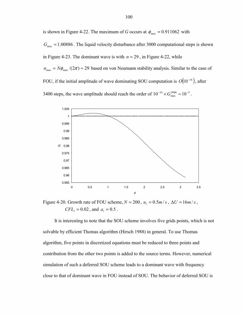
100
is shown in Figure 4-22. The maximum of G occurs at 911062.0max =φ with
00886.1max =G . The liquid velocity disturbance after 3000 computational steps is shown
in Figure 4-23. The dominant wave is with 29=n , in Figure 4-22, while
29)2/(maxmax ≈= πφNn based on von Neumann stability analysis. Similar to the case of
FOU, if the initial amplitude of wave dominating SOU computation is ( )1610−O , after
3400 steps, the wave amplitude should reach the order of 53000max
16 1010 −− ≈×G .
0.955
0.96
0.965
0.97
0.975
0.98
0.985
0.99
0.995
1
1.005
0 0.5 1 1.5 2 2.5 3 3.5
φ
G
Figure 4-20. Growth rate of FOU scheme, 200=N , smul /5.0= , smU /16=∆ ,
02.0=lCFL , and 5.0=la .
It is interesting to note that the SOU scheme involves five grids points, which is not
solvable by efficient Thomas algorithm (Hirsch 1988) in general. To use Thomas
algorithm, five points in discretized equations must be reduced to three points and
contribution from the other two points is added to the source terms. However, numerical
simulation of such a deferred SOU scheme leads to a dominant wave with frequency
close to that of dominant wave in FOU instead of SOU. The behavior of deferred SOU is

101
unpredictable by von Neumann analysis. To obtain the solution of two-fluid model with
SOU authentically, an iteration method is employed in this study to ensure that the
variables at the new time step are solved simultaneously. Although the method is not
efficient for the application of two-fluid model, it is employed in this study for the
purpose of assessing the performance of SOU scheme.
4.1.5.4 Discussion on the growth of short wave
In the last section, it is seen that the undesirable short waves emerge from the
computation and destroy the original information in the computational domain because of
numerical instability. This numerical instability is the character of numerical scheme and
influenced by the ill-posedness of two-fluid model. Preliminary analysis shows that the
unwanted short waves come from computer’s machine round–off error, but the growth
history of short wave is still not clear.
In order to clearly demonstrate how the short wave emerges and develops during
computation, another numerical experiment is conducted. For the FOU scheme used in
the last section for Figure 4-20 and 4-21, a series of computations is carried out using
successively decreasing initial amplitude (from sm /10 4− to sm /10 12− ) for the liquid
velocity disturbance lu . The growth of the amplitude of lu as a function of time is
recorded for each initial amplitude while all other physical and computational parameters
are fixed. Figure 4-24 shows the variations of the wave amplitude for all values of initial
disturbance amplitude in lu .
In Figure 4-24, it is observed that during the initial stage, all amplitudes grow
according to the G (k=2π) in the form of nG0ε in which 0ε is the initial amplitude of the
disturbance, G is the growth rate at k=2π based on von Neumann analysis, and n denotes

102
nth time step. Since the short wave grows out of the machine round-off error
independently in the form of nrGmaxε in which ( )1610~ −Orε is the amplitude of the
round-off error whose exact value is uncertain, and 00201.1max =G is the maximum
growth rate for the FOU scheme for the present condition obtained from the von
Neumann analysis. It corresponds to maxφ = 0.586903. Clearly, smaller value of 0ε
requires less time (or small n) for the round off error to take over the primary wave
(k=2π). The envelope of these computed amplitudes seem to agree well with the nrGmaxε
denoted by the thick dash line in Figure 4-21 with an estimated value of 16102 −×=rε .
-2.00E-05
-1.50E-05
-1.00E-05
-5.00E-06
0.00E+00
5.00E-06
1.00E-05
1.50E-05
2.00E-05
0 0.1 0.2 0.3 0.4 0.5 0.6 0.7 0.8 0.9 1
x(m)
Dis
turb
ance
(m/s
)
Figure 4-21. lu using FOU scheme after 12000 steps of computation. 200=N ,
smul /5.0= , smU /16=∆ , 02.0=lCFL , and 5.0=la .

103
0.8
0.85
0.9
0.95
1
1.05
0 0.5 1 1.5 2 2.5 3 3.5
φ
G
Figure 4-22. Growth rate of SOU scheme. 200=N , smul /1= , smU /16=∆ ,
05.0=lCFL , and 5.0=la .
-4.00E-04
-3.00E-04
-2.00E-04
-1.00E-04
0.00E+00
1.00E-04
2.00E-04
3.00E-04
4.00E-04
0 0.1 0.2 0.3 0.4 0.5 0.6 0.7 0.8 0.9 1
x(m)
Dis
turb
ance
(m/s
)
Figure 4-23. lu using SOU scheme after 3000 steps of computation. 200=N ,
smul /1= , smU /16=∆ , 05.0=lCFL , and 5.0=la .

104
As computation continues, the wave amplitudes in Figure 4-24 do not become
unbound. This is different from the case with the use of CDS in Figure 4-19. The
difference stems from the following:
1. High numerical diffusion of FOU scheme causes decrease of U∆ .
2. When the disturbance amplitude becomes O(1), the based flow parameters are changed. The nonlinear effects in the discretized system of equations become strong so that the numerical solution may have evolved to a different stable state. The result of von Neumann analysis is no longer applicable.
1.00E-16
1.00E-15
1.00E-14
1.00E-13
1.00E-12
1.00E-11
1.00E-10
1.00E-09
1.00E-08
1.00E-07
1.00E-06
1.00E-05
1.00E-04
1.00E-03
1.00E-02
1.00E-01
1.00E+00
0 0.5 1 1.5 2 2.5 3 3.5 4
t(s)
Am
plitu
de(m
/s)
growth of round-off error
Figure 4-24. Growth history of lu under different initial amplitude using FOU scheme.
4.1.5.5 Wave development resulting from disturbance at inlet
In the comparison of last section, periodic boundary conditions are used to match
the requirement of von Neumann stability analysis. However, the applications of
two-fluid model are not limited to periodic boundary conditions. In this section, wave
propagation developed from an inlet disturbance is studied. The growth rate of the
disturbance depends on the flow parameter and the numerical scheme. Initially small

105
sinusoidal waves for lα , lu and gu with π24×=k satisfying Equation (4.49) is
introduced at st 0= . At the inlet, the boundary conditions of lα , lu and gu with
π24×=k satisfying Equation (4.49) is posed as function of t. At the outlet, 2nd order
extrapolation is employed.
Figure 4-25 shows the growth of inlet disturbance by FOU scheme under
well-posed condition. The computational parameters are 200=N , smul /1= ,
smug /17= , 0=β , 05.0=lCFL , and 5.0=la . The flow is well-posed and scheme is
unstable for low frequency wave. Figure 4-25 clearly shows the exponential growth of a
low k wave, as it propagates to the down stream. The flow under similar parameters but
smug /21= is shown in Figure 4-26. The flow is ill-posed with these parameters. The
major difference between the Figure 4-25 and Figure 4-26 is that the wave growth rate in
Figure 4-26 is much larger than that in Figure 4-25. If the computational domain is longer
enough, both computations will break down. All the behavior of waves in Figure 4-25
and Figure 4-26 agrees with the von Neumann stability analysis.
Next, inlet disturbance growth with CDS scheme is studied. In Figure 4-27, the
computational parameters are the same as those in Figure 4-25. It is shown that from inlet
to outlet, the wave grows slowly. This reflects the accuracy of the CDS scheme. The
wiggle on the wave is due to the extrapolated downstream boundary conditions. Because
it is not a non-reflection boundary condition, high frequency waves are generated at
downstream boundary and propagate upstream until they are bounced back by upstream
boundary. Low damping rate of CDS scheme allows the high frequency waves to exist
for a long time in the computational domain. Figure 4-28 shows the flow under same
computational parameter as in Figure 4-26. Since the flow is ill-posed, the wave grows so

106
fast that the computation breaks down while the disturbance has not reached the middle
of domain. Comparison between the Figure 4-26 and Figure 4-28 shows that CDS
scheme is less stable than the FOU scheme if the velocity difference is notably higher
than the IKH stability criterion. This is confirmed by the comparison of growth rate of
FOU and CDS (Figure 4-29) at the condition of Figure 4-26 and Figure 4-28. This feature
suggests that the FOU scheme is preferred to the CDS scheme if the velocity difference
between gas and liquid phase is extremely large.
4.1.6 Conclusions
Numerical instability for the incompressible two-fluid model near the ill-posed
condition is investigated for various cell face interpolation schemes, while the pressure
correction method is used to obtain the pressure, volume fraction and velocities. The von
Neumann stability analysis is carried out to obtain the growth rate of a small disturbance
in the discretized system. The central difference scheme has the best stability
characteristics in handling the two-fluid model, followed by the QUICK scheme. It is
quite interesting to note that the excessive numerical diffusion in the 1st order upwind
scheme seems to promote the numerical instability in comparison with the central
difference scheme. Despite its nominal 2nd order accuracy and popularity, the 2nd order
upwind scheme is much more unstable than the 1st order upwind scheme for solving two-
fluid model equations. Different discretization schemes for the convection term with
varying degrees of numerical diffusion and dispersion cannot cause a delay the onset of
instability; they often promote instability in the two-fluid model.

107
-5.00E-06
-4.00E-06
-3.00E-06
-2.00E-06
-1.00E-06
0.00E+00
1.00E-06
2.00E-06
3.00E-06
4.00E-06
5.00E-06
6.00E-06
0 0.1 0.2 0.3 0.4 0.5 0.6 0.7 0.8 0.9 1
x(m)
Dis
turb
ance
(m/s
)
Flow direction
Figure 4-25. lu propagates in the pipe with FOU at well-posed condition, quasi-steady
state.
-3.00E-03
-2.00E-03
-1.00E-03
0.00E+00
1.00E-03
2.00E-03
3.00E-03
4.00E-03
0 0.1 0.2 0.3 0.4 0.5 0.6 0.7 0.8 0.9 1
x(m)
Dis
turb
ance
(m/s
)
Flow direction
Figure 4-26. lu propagates in the pipe with FOU scheme at ill-posed condition, quasi-
steady state.

108
-1.50E-06
-1.00E-06
-5.00E-07
0.00E+00
5.00E-07
1.00E-06
1.50E-06
0 0.1 0.2 0.3 0.4 0.5 0.6 0.7 0.8 0.9 1
x(m)
Dis
turb
ance
(m/s
)
Flow direction
Figure 4-27. lu propagates in the pipe with CDS at well-posed condition, quasi-steady
state.
-1.00E-01
-5.00E-02
0.00E+00
5.00E-02
1.00E-01
1.50E-01
0 0.1 0.2 0.3 0.4 0.5 0.6 0.7 0.8 0.9 1
x(m)
Dist
urba
nce(
m/s
)
Flow direction
Figure 4-28. lu propagates in the pipe with CDS at ill-posed condition, an instance
before the computation breaks down.

109
0.88
0.9
0.92
0.94
0.96
0.98
1
1.02
0 0.5 1 1.5 2 2.5 3 3.5
φ
G FOU
CDS
Figure 4-29. Comparison of growth rate between CDS and FOU schemes. 200=N ,
smul /1= , smug /21= , 05.0=lCFL , and 5.0=la .
The analytically predicted wave amplitude growth rate is also compared with that
obtained from carefully implemented computations using various discretization schemes
for the convection term. Excellent agreement between the numerical results and the
predicted results is obtained for the growth of the wave amplitude and the dominant
wavenumber when the computation becomes unstable. Inlet disturbance growth test
shows the pressure correction scheme can correctly capture two-phase flow in the
pipeline.
The relation between computational instability and ill-posedness is discussed. In
the presence of a small-amplitude long-wave disturbance, whose amplitude is much
larger than the machine round-off error, the growth of the disturbance exactly matches
the prediction of the von Neumann stability analysis when the computational stability
condition is violated. In the meantime, a shorter wave emerges from the machine round-
off error, and eventually dominates the entire disturbance, which causes the computation

110
to blow up. This computational instability is widely interpreted as the result of ill-
posedness of the two-fluid model. The results of the present study suggest that the
computational instability is largely the property of the discretized two-fluid model and is
strongly affected by the inherent ill-posedness of the two-fluid model differential
equations. Introduction of numerical diffusion and/or dispersion can significantly change
the instability of the discretized system; however, such steps often yield unfavorable
computational results. For solving two-fluid models, central difference is recommended
since it is much more accurate and dependable than other schemes investigated.
4.2 Viscous Two-Fluid Model
4.2.1 Introduction
Inviscid two-fluid model suffers from the ill-posdness problem, which coincides
with the invicid Kelvin-Helmholtz instability. It is known that IKH instability in the
stratified flow implies that the stratified flow is unstable and transition of flow regimes
will occur. The transition can be from stratified flow to slug flow or stratified flow to
annular flow, depending on other flow parameters (Taitel and Dukler, 1976; Barnea and
Taitel, 1994). However, the instability of viscous two-phase flow in pipe flow, which can
be described by viscous two-fluid model, comes earlier than the IKH stability in the pipe
flow. Lin and Hanratty (1986, 1987) distinguished the viscous Kelvin-Helmholtz stability
(VKH) from the inviscid Kelvin-Helmholtz stability. They also showed that the transition
from stratified flow to slug flow is governed by the VKH stability analysis instead of the
IKH stability analysis and that the VKH instability is triggered earlier than the IKH
instability. In the region where the two-phase flow is VKH unstable but IKH stable, the
two-fluid model is well-posed. Issa and Kempf (2003) attempted to simulate the VKH
instability under the well-posed condition using the two-fluid model. They qualitatively

111
captured VKH instability and the transition from stratified flow to slug flow. However,
the numerical accuracy of their scheme under the VKH unstable condition is uncertain. In
the last section, von Neumann stability analysis of the two-fluid model clearly shows that
the flow with the IKH instability cannot be accurately captured by the numerical solution
because of the indefinite growth of the disturbance under an unstable condition.
In this section, the numerical instability of the viscous two-fluid model will be
investigated using von Neumann stability analysis and the relation between the numerical
instability and the VKH instability of viscous two-fluid model will be clarified.
Furthermore, the wave growth rate obtained using the von Neumann stability analysis is
used to validate the numerical scheme for the viscous two-fluid model.
4.2.2 Governing Equations
In the viscous two-fluid model, as shown in Figure 4-30, the viscosity of fluid
appears in the shear stresses in source terms in the fluid momentum equations. Other
assumptions are the same as that of inviscid two-fluid model presented in the previous
section. There is no mass transfer between the gas phase and liquid phase, and the surface
tension between the two phases is neglected. Both phases are incompressible. Hence, the
governing equations are as follows:
Pipe cross section
Liquid phase
Gas phase
Interface
Liquid velocity lu
Gas velocity gu
Gravity g
Gas velome faction gα
Liquid velome faction lα
gτ
iτ
iτ
lτ
Figure 4-30. Schematic depiction of viscous two-fluid model.

112
( ) ( ) 0=∂∂+
∂∂
lll uxt
αα , (4.49)
( ) ( ) 0=∂∂+
∂∂
ggg uxt
αα , (4.50)
( ) ( )l
ii
l
lll
ll
i
l
lllll A
SA
Sg
xHg
xp
ux
ut ρ
τρ
τβααβρααα +−−
∂∂
−∂∂
−=∂∂+
∂∂ sincos2 , (4.51)
( ) ( )g
ii
g
ggg
lg
i
g
ggggg A
SA
Sg
xHg
xp
ux
ut ρ
τρ
τβααβ
ρα
αα −−−∂∂
−∂∂
−=∂∂+
∂∂ sincos2 . (4.52)
To close the two-fluid model, the correlations for shear stress must be specified. In
this study, the correlations used by Barnea and Taitel (1994) are adopted, as shown in
Equations 2.20 to 2.27.
4.2.3 Theoretical Analysis
4.2.3.1 Characteristics and ill-posedness
The characteristic analysis for the inviscid two-fluid model shows that the
characteristic roots may be complex, which leads to ill-posedness. Similar analysis can be
applied on the viscous two-fluid model.
Equations 4.49 to 4.52 can be written in vector form as
][][][ Cx
Bt
A =∂∂+
∂∂ UU , (4.53)
where [A], [B] and [C] are coefficient matrices given by
−
−=
000000010001
][
gg
ll
uu
A
αα
, (4.54a)

113
+−
+
−
=
g
ggggg
l
lllll
gg
ll
ugHu
ugHu
uu
B
ρα
αβ
ρααβ
αα
20cos
02cos
0000
][
2
2 , (4.54b)
[ ]
−−−
+−−=
g
ii
g
ggg
l
ii
l
lll
AS
AS
g
AS
AS
gC
ρτ
ρτ
βα
ρτ
ρτβα
sin
sin00
, (4.54c)
The characteristic roots λ of the system are determined by the following:
0][][ =− BA λ . (4.55)
The only difference between the characteristic equation for the inviscid two-fluid
model and that for viscous two-fluid model are the friction terms in vector [ ]C . However,
Equation (4.55) shows that the characteristics are not affected by vector [ ]C . Thus,
viscous terms in the viscous two-fluid model do not affect the characteristics of the
two-fluid model. The criterion for ill-posedness for viscous two-fluid model remains the
same as that for the inviscid two-fluid model. However, the viscous effect in [ ]C can
affect the linear stability of the viscous two-fluid model to cause flow regime transition.
4.2.3.2 Viscous Kelvin-Helmholtz (VKH) analysis and linear instability
It is known that stability of interface between the liquid phase and gas phase is
attributed to the viscous Kelvin-Helmholtz instability. Barnea and Taitel (1994) showed
that the velocity difference between two phases under VKH instability is less than that
under IKH instability. Flow regime transition starts when the flow encounters VKH
instability rather than IKH instability. VKH analysis provides not only a stability

114
condition for the linearized viscous two-fluid model, but also gives growth rate of
infinitesimal disturbance in the viscous two-fluid model.
Governing equations (Equations 4.49-4.52) are linearized and substituted for the
perturbed liquid volume fraction, liquid and gas phase velocities, and pressure given by
Equation (4.15) (Barnea and Taitel, 1994). The following system is obtained for the
disturbance amplitude, ( )Tpgl εεεε ,,, :
( )
( )
0
cos
cos
0000
=
−∂∂
+−∂∂
∂∂
+−
−∂∂
∂∂
+−∂∂
+−
−−−
p
g
l
g
ggg
l
g
l
gg
l
l
g
l
l
lll
l
ll
l
l
gg
ll
kuF
ikuuF
iF
igHk
kuFi
uFikuFigHk
kkukku
εεεε
ωρα
βρα
ωρα
βρα
αωαω
. (4.56)
For non-trivial solutions to exist, the following dispersion equation for ω must hold
( ) 02 22 =−+−− ekickbiak ωω , (4.57)
where
+=
g
gg
g
ll uua
αρ
αρ
ρ1 , (4.58a)
∂∂−
∂∂=
ggll uF
uFb
ααρ11
21 , (4.58b)
( )
−−+= βρρ
ααρ
αρ
ρcos1 22
gHuuc gll
l
g
gg
l
ll , (4.58c)
∂∂+
∂∂+
∂∂−−=
lgg
g
ll
l FuFu
uFu
eαααρ
1 , (4.58d)
where
gl FFF += , (4.59)

115
and
βρα
τα
τsing
AS
AS
F ll
ii
l
lll −+−= , (4.60)
βρα
τα
τsing
AS
AS
F gg
ii
g
ggg −−−= . (4.61)
Therefore, dispersion relation between wave angular velocity ω and wavenumber k is
obtained as
( ) ( ) ( )iabkekbkcabiak 2222 −+−−±−=ω . (4.62)
The negative imaginary part of ω determines the growth rate of disturbance.
4.2.4 Analysis on Computational Intability
4.2.4.1 Description of numerical methods
Governing equations (Equations 4.49 to 4.52) are solved iteratively by the pressure
correction scheme introduced in Section 4.2.3 with minor modification to include
shear stress terms. The finite volume method and staggered grid were used to
discretize the governing equations. We used the Euler backward scheme to discretize the
transient term.
Therefore, the liquid continuity equation (Equation 4.49) is integrated over the
main control volume. The discretized equation is the same as Equation 4.20.
Next the liquid momentum equation (Equation 4.50) is integrated over the
velocity control volume.
( ) ( )( ) ( ) ( ) ( ) ( )( ) ( ) ( ) ( )( ) ( ),,,cos
0
gllll
llelwlew
l
Pl
wllwlellelPllPll
uuFgHpp
uuuuuutx
αραβαα
ρα
αααα
+−+−
=−+−∆∆
(4.63)

116
The cell face flux is liquid velocity, which is obtained by central difference, and the
volume fraction and liquid velocity at the cell face can be interpolated using central
difference, 1st order upwind, 2nd order upwind, and QUICK.
Using similar discretization procedure, the gas phase momentum equation is
integrated:
( ) ( )( ) ( ) ( ) ( ) ( )( ) ( ) ( ) ( )( ) ( ),,,cos
0
gllgg
ggelwlew
g
Pg
wggwgeggegPggPgg
uuFgHpp
uuuuuutx
αρα
βααρα
αααα
+−+−
=−+−∆∆
(4.64)
For pressure correction scheme, the total mass constrain equation is the same as
Equation (4.26). The final pressure equation is obtained by substituting two momentum
equations, Equation (4.51) and Equation (4.52), into the discretized total mass constrain
equation that is the same as Equation (4.26).
4.2.4.2 Von Neumann stability analysis for various convection schemes
Generally, the von Neumann stability analysis for viscous two-fluid model is
similar to that for inviscid two-fluid model. FOU is employed as an illustrative example.
Both the liquid and gas velocities are assumed positive for simplicity and practical
purpose.
The wave growth equations for the liquid and gas mass conservation equations are
the same as those in the inviscid two-fluid model
( ) ( ) ( ) 011 21
211 =−+
−+−∆∆ −−− φφφ αεε II
llI
l eeeuGtx (4.65)
( ) ( ) ( ) 011 21
211 =−−
−+−∆∆ −−− φφφ αεε II
ggI
g eeeuGtz
(4.66)
For liquid momentum equation, Equation (4.51) is discretized with FOU scheme,

117
( ) ( ) ( ) ( )( ) ( ) ( ) ( )( )
( ) ( ) ( ) ( )( ) ( ) ( ) ( ) ( ).,,cos 2
1
21
21
21
21
21
21
21
21
21
21
11
1
11
xuuaFHgpp
uuuuxt
uu
l
niln
ignil
nill
nil
nill
ni
ni
l
nil
nill
nil
nill
nil
nil
nil
nil
nil
∆
+−+−=
−+∆∆
−
+
+++++
+
−++
−+
−+++
ρ
αααβ
ρ
α
αααα
(4.67)
For the gas phase, the velocity variable is governed with the following equation
( ) ( ) ( ) ( )( ) ( ) ( ) ( )
( )( ) ( ) ( )( ) ( ) ( ) ( )
( ).,,cos 2
1
21
21
21
21
21
21
21
21
21
21
11
1
11
xuuaFHgpp
uuuuxt
uu
g
nign
ignil
nilg
nil
nilg
ni
ni
g
nig
nigg
nig
nigg
nig
nig
nig
nig
nig
∆
+−+−=
−+∆
∆
−
+
++++++
−++
−+
−+++
ρ
αααβ
ρ
α
αααα
(4.68)
Combining Equations (4.67-68) to cancel the pressure term and linearizing lead to.
( ) ( )( ) ( ) ( )
( ) ( )( ) ( ) ( )
( ) ( ) ( )( ) ( ) ( ) ( ) .ˆˆˆˆˆcos
ˆˆˆˆ
ˆˆˆˆ
21
21
21
21
21
21
21
21
21
21
21
1
11
xFuuFu
uFH
g
uuuuuu
uuuutx
nil
l
nig
g
nil
l
nil
nil
l
lgl
nig
niggg
nil
nilll
nig
nigg
nil
nill
∆
∂∂+
∂∂+
∂∂+−−=
−−−+
−−−
∆∆
++++
−+−+
−++
−++
αα
ααα
βρρ
ρρ
ρρ
(4.69)
Substituting wave components, Equation (4.32), into Equation (4.69) leads to
( ) ( )( ) ( )
( ) ( ) .011
11
2cos
1
1
21
21
21
21
=
∆
∂∂+−+−
∆∆−
∆
∂∂−−+−
∆∆+
+∆∂∂−−−
−−
−−
−−
xuFeuG
tx
xuFeuG
tx
eexFeeH
g
g
Igggg
l
Illll
II
l
II
l
lgl
φ
φ
φφφφ
ρρε
ρρε
ααβρρε
(4.70)
Equation (4.65, 4.66, 4.79) can be written in a matrix form as

118
( ) ( ) ( )( ) ( ) ( )
( ) ( ) ( )( )
( )( )
0
1
1
1
1
2
cos
011
011
11
1
1
21
21
21
21
21
21
21
21
=
∆∂∂−
−+
−∆∆
∆∂∂−
−+
−∆∆
−
+∆∂∂−
−′−
−−+−∆∆
−−−+−∆∆
−
−
−
−
−
−
−−−
−−−
l
g
l
Il
l
g
Ig
g
II
l
IIlgl
IIl
Il
IIg
Ig
xuF
eu
Gtx
xuF
eu
Gtx
eexF
eeg
eeeuGtx
eeeuGtx
εεε
ρρ
α
αβρρ
α
α
φφφφ
φφ
φφφ
φφφ
. (4.71)
Non-trivial solutions for ( )Tlg εεε ,, exist only when the determinant of the matrix
is zero. Hence, the equation for the growth rate G shares the same form as the inviscid
two-fluid model growth rate equation but with different coefficients:
( ) ( ) 0121 =++ −− cGbGa , (4.72)
where
ρ=a , (4.73a)
( )( ) ( )( )
∂∂−
∂∂∆+
∆++∆+−=
llggl
l
lg
g
g
uF
uFtCFLCFLb
ααφ
αρφ
αρ 11112 , (4.73b)
( )( ) ( )( )
( )
( )( ) ( )( ),11sin
2sin4cos
11
22
22
φα
φαα
φ
φα
βρρ
φαρφ
αρ
∆+∂∂∆−∆+
∂∂∆+
∂∂∆
∆∆+
−
∆∆+
∆++∆+=
lll
gggl
l
lgl
ll
lg
g
g
CFLuFtCFL
uFtFt
xtI
Hg
xt
CFLCFLc
(4.73c)
The values of ( )φ∆ in Equation (4.73) are given in Table 4-2. Comparing with Equation
(4-46 a-c), Equations (4.73a-c) shows additional terms representing the influence of wall
shear stress on the wave growth rate.
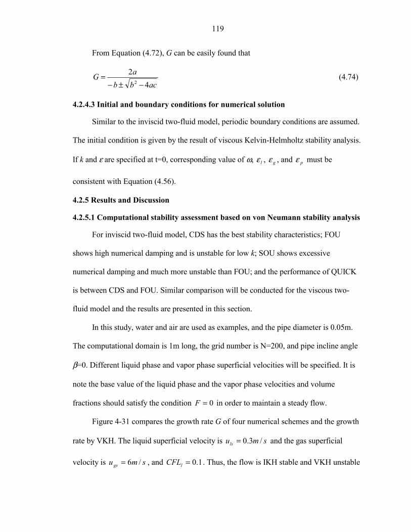
119
From Equation (4.72), G can be easily found that
acbbaG
42
2 −±−= (4.74)
4.2.4.3 Initial and boundary conditions for numerical solution
Similar to the inviscid two-fluid model, periodic boundary conditions are assumed.
The initial condition is given by the result of viscous Kelvin-Helmholtz stability analysis.
If k and ε are specified at t=0, corresponding value of ω, lε , gε , and pε must be
consistent with Equation (4.56).
4.2.5 Results and Discussion
4.2.5.1 Computational stability assessment based on von Neumann stability analysis
For inviscid two-fluid model, CDS has the best stability characteristics; FOU
shows high numerical damping and is unstable for low k; SOU shows excessive
numerical damping and much more unstable than FOU; and the performance of QUICK
is between CDS and FOU. Similar comparison will be conducted for the viscous two-
fluid model and the results are presented in this section.
In this study, water and air are used as examples, and the pipe diameter is 0.05m.
The computational domain is 1m long, the grid number is N=200, and pipe incline angle
β=0. Different liquid phase and vapor phase superficial velocities will be specified. It is
note the base value of the liquid phase and the vapor phase velocities and volume
fractions should satisfy the condition 0=F in order to maintain a steady flow.
Figure 4-31 compares the growth rate G of four numerical schemes and the growth
rate by VKH. The liquid superficial velocity is smuls /3.0= and the gas superficial
velocity is smugs /6= , and 1.0=lCFL . Thus, the flow is IKH stable and VKH unstable

120
based on theoretical analyses. The VKH growth rate curve is flat and slightly higher than
one. The growth rate of CDS is slightly lower than one but quite close to one, except at
the low k, where G>1. FOU scheme possesses excessive numerical damping at high k.
SOU shows larger numerical damping than FOU at high k. Performance of QUICK
scheme is between CDS and FOU. The results of Figure 4-31 generally agree with those
of inviscid two-fluid model. However, shear stresses cause the flow instability to occur at
lower k in viscous flow. The instability associated with the shear stresses is further
illustrated in Figure 4-32, which is the enlarged low k part of Figure 4-28.
0.75
0.8
0.85
0.9
0.95
1
1.05
0 0.5 1 1.5 2 2.5 3 3.5φ
G
VKH
CDS
QUICK
FOU
SOU
Figure 4-31. Comparisons of growth rate of different schemes. 200=N , smuls /3.0= ,
smugs /6= ,and 1.0=lCFL .
Figure 4-32 shows that at extreme low k the growth rates of all the schemes agree
well with prediction of the VKH analysis, but when the k is slightly larger, the G profile
quickly deviates from growth rate of the VKH analysis. If the flow instability are to be
captured, the grid has to be extreme fine to keep the wave triggering flow instability
locate at low φ, which is xk ∆* . It is shown in Figure 4-32 that the FOU curve is far from

121
CDS, SOU and QUICK. This reflects that 1st order accuracy FOU and the other three
schemes all have 2nd order accuracy.
0.998
0.9985
0.999
0.9995
1
1.0005
0 0.1 0.2 0.3 0.4 0.5φ
G
VKH
CDS
QUICK
FOUSOU
Figure 4-32. Comparisons of growth rate of different schemes at low k. 200=N ,
smuls /3.0= , smugs /6= ,and 1.0=lCFL .
Next, the effect of fluid viscosity on the numerical stability is presented. Because
the liquid viscosity has more influence on the stability of two-phase flow than the gas
viscosity (Barnea and Taitel, 1994), the investigation focuses on the influence of the
liquid viscosity.
Figure 4-33 compares the growth rate of viscous and inviscid two-fluid model with
CDS for air-water system. The viscosity of water is sPawater *10855.0 3−×=µ . The flow
is IKH stable and VKH unstable. The growth rate based on the VKH analysis is slightly
higher than one. Due to the numerical damping, the major part of G of viscous two-fluid
model is below one, except at low k. Compared with the growth rate of inviscid two-fluid
model, the effect of shear stresses on the growth rate is clearly shown. Shear stresses

122
result in low G for the middle and high range of k and high G for low range of k. The fact
that 1>G in the low k range leads to the instability of numerical scheme.
0.992
0.993
0.994
0.995
0.996
0.997
0.998
0.999
1
1.001
0 0.5 1 1.5 2 2.5 3 3.5
φ
G
viscous inviscid
VKH
IKH
Figure 4-33. Growth rate for CDS scheme with VKH unstable. 200=N , smuls /3.0= ,
smugs /6= ,and 1.0=lCFL .
Figure 4-34 shows the effect of liquid viscosity on the growth rate. The fluid
system is still air-water, but the viscosity of water is given as sPawater *10 2−=µ . This
viscosity is much higher than the typical viscosity of water used in Figure 4-33. Thus, the
growth rate based on the VKH analysis is much higher than that in Figure 4-33. The
difference between the viscous and inviscid growth rate in Figure 4-31 is larger than that
in Figure 4-33. Beside the value of G, the k range of unstable harmonics in Figure 4-34 is
larger than that in Figure 4-33.
Figure 4-35 shows the amplification factor of air-water system with
sPawater *10 1−=µ . This viscosity is one order of magnitude higher than the viscosity
used in Figure 4-34. To keep the flow VKH unstable and IKH stable, the liquid and gas

123
phase superficial velocities are adjusted to smuls /1.0= , and smugs /2= . To keep both
the liquid and gas Courant number moderate, 01.0=lCFL is used. It is shown in Figure
4-35 that unstable range of k is much larger than ranges in Figure 4-33 and Figure 4-34.
However, the difference between the viscous growth rate and inviscid growth rate is not
significantly larger than those in Figure 4-33 and Figure 4-34. Thus, the shear stresses
effect is only significant at the low k range or long waves.
0.992
0.993
0.994
0.995
0.996
0.997
0.998
0.999
1
1.001
0 0.5 1 1.5 2 2.5 3 3.5
φ
G
VKH
viscous Inviscid
IKH
Figure 4-34. Growth rate for CDS scheme with VKH instability. sPawater *10 2−=µ , 200=N , smuls /3.0= , smugs /6= ,and 1.0=lCFL .
Next, the effect of shear stresses on FOU scheme is presented. It is known that the
numerical damping of FOU scheme is much higher than that of CDS scheme. Even in
CDS scheme with low numerical damping, when the flow is VKH unstable, the
numerical damping effect still makes G less than one at middle and high k due to
numerical damping, as shown in Figure 4-32. Since numerical damping of FOU is much
higher than that of CDS, it is anticipated that the numerical effect of FOU is much more

124
substantial in viscous two-fluid model. Figure 4-36 shows that the growth rate of FOU
for both the viscous and inviscid two-fluid models. The computational parameters are the
same as those used in Figure 4-33. It is shown that the viscous and inviscid growth rate
curves are quite close to each other and G of viscous model is slightly larger. Only at low
k, shear stresses effect makes significant difference between viscous and inviscid model.
The growth G of viscous model exceeds one, and flow instability is thus triggered.
0.992
0.993
0.994
0.995
0.996
0.997
0.998
0.999
1
1.001
0 0.5 1 1.5 2 2.5 3 3.5
φ
G
VKH
viscous
InviscidIKH
Figure 4-35. Growth rates for CDS scheme with VKH instability. sPawater *10 1−=µ ,
200=N , smuls /1.0= , smugs /2= ,and 01.0=lCFL .
Figure 4-37 shows the growth rate of FOU scheme with higher liquid viscosity.
The computational parameters are the same as that used in Figure 4-35. It is clearly
shown that the choice of numerical scheme has a much larger impact on the stability of
the computation, and the physical viscous effect is less significant.
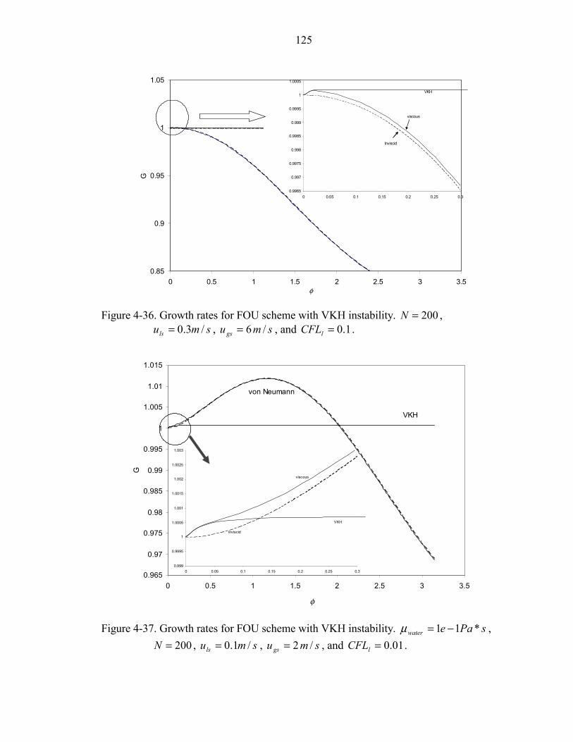
125
0.8
0.85
0.9
0.95
1
1.05
0 0.5 1 1.5 2 2.5 3 3.5φφφφ
G
0.85
0.9
0.95
1
1.05
0 0.5 1 1.5 2 2.5 3 3.5
G
0.9965
0.997
0.9975
0.998
0.9985
0.999
0.9995
1
1.0005
0 0.05 0.1 0.15 0.2 0.25 0.3
VKH
viscous
Inviscid
φ
Figure 4-36. Growth rates for FOU scheme with VKH instability. 200=N ,
smuls /3.0= , smugs /6= , and 1.0=lCFL .
0.965
0.97
0.975
0.98
0.985
0.99
0.995
1
1.005
1.01
1.015
0 0.5 1 1.5 2 2.5 3 3.5
G
VKH
von Neumann
0.999
0.9995
1
1.0005
1.001
1.0015
1.002
1.0025
1.003
0 0.05 0.1 0.15 0.2 0.25 0.3
VKH
viscous
inviscid
φ
Figure 4-37. Growth rates for FOU scheme with VKH instability. sPaewater *11 −=µ ,
200=N , smuls /1.0= , smugs /2= , and 01.0=lCFL .

126
4.2.5.2 Computational assessment based on the growth of disturbance
To validate the pressure correction scheme for the viscous two-fluid model,
comparisons between the computed wave growth rate and the analytical growth rate
predicted using the von Neumann stability analysis are presented.
In this section, the fluids used still are water and air, and pipe diameter is 0.05m.
The computational domain is 1m long the grid number N=200. To maintain periodic
boundary conditions for the viscous flow, the base values of the fluid volume fractions,
the liquid and gas phase velocities, and the pipe incline angle should satisfy both 0=lF
and 0=gF . Through solving these two force balance equations, the flow parameters are
obtained. Initial conditions are compatible with the result of the VKH analysis, and the
analytical solution of disturbance growth is also obtained from the VKH analysis.
Figure 4-38 shows the growth history of a harmonic with π2=k by CDS. The
parameters used are smul /2= , smug /0.998174= , -0.0617144=β , and 98.0=la .
The flow is well-posed and VKH unstable. The disturbance grows exponentially as
shown in Figure 4-38. The correctness of the numerical scheme can be verified by
comparing the numerical growth rate with the growth rate predicted using the von
Neumann stability analysis. Based on the von Neumann stability analysis, the predicted
amplitude ratio from st 0= to st 10= is 174.75, and the computed amplitude ratio is
176.86. The error is 1.21% in 10 seconds. Furthermore, the growth history based on the
VKH analysis is also plotted in Figure 4-38. The growth rate for each time step using the
VKH analysis is 1.00006491 and the growth rate for each time step using von Neumann
analysis is 1.00006454. It is not surprising because the CDS has excellent numerical
accuracy when it is applied to two-fluid model. In the final stage of growth, because the

127
amplitude of the wave is no longer a small value, the assumption of the von Neumann
stability analysis and the VKH instability analysis becomes invalid. Thus, the waves enter
non-linear growth stage and the numerical growth rate no longer matches the analytical
one.
1.00E-06
1.00E-05
1.00E-04
1.00E-03
1.00E-02
1.00E-01
0 2 4 6 8 10 12 14 16 18 20
t(s)
Ampl
itude
(m/s
)
VKH
Numerical
Figure 4-38. Growth history of lu using CDS scheme. 200=N , smul /2= ,
smug /0.998174= , -0.0617144=β , 98.0=la , and 05.0=lCFL .
With the same computational parameters, the growth history of FOU is shown in
Figure 4-39. The growth rate based on the VKH analysis for each time step is still
1.00006491 but the growth rate based on the von Neumann for each time step for FOU is
only 1.00004197, which is much smaller than that using VKH analysis. The low growth
rate is the result of numerical damping of FOU. Figure 4-39 presents the discrepancy in
the amplitude growth between the VKH prediction and FOU scheme. The correctness of
the numerical scheme can be verified using comparing the computed growth rate with
predicted growth rate based on the von Neumann stability analysis. By the von Neumann

128
stability analysis, the total amplitude ratio from st 0= to st 10= is 28.7333 and the
computed total growth ratio is 28.3785. The error is 1.23% in 10s.
1.00E-06
1.00E-05
1.00E-04
1.00E-03
1.00E-02
1.00E-01
0 2 4 6 8 10 12 14 16 18 20t(s)
Am
plitu
de(m
/s)
VKH
Numerical
Figure 4-39. Growth history of lu using FOU scheme. 200=N , smul /2= ,
smug /0.998174= , -0.0617144=β , 98.0=la , and 05.0=lCFL .
In this section, the computed G is compared with the predicted G using von
Neumann stability analysis. The comparisons show that the pressure correction scheme is
quite accurate and verifies that the FOU possesses excessive numerical damping, while
the CDS has better numerical accuracy for the viscous two-fluid model.
4.2.5.3 Wave development resulting from disturbance at inlet
In the previous section, periodic boundary conditions are used to match the
requirement of von Neumann stability analysis. However, the applications of the two-
fluid model are not limited to periodic boundary conditions. In this section, an inlet
boundary condition is specified and the wave propagation is predicted using the viscous
two-fluid model. Similar to the initial condition in the inviscid two-fluid model, at st 0= ,

129
small sinusoidal waves for lα , lu and gu with π24×=k satisfying Equation (4.56) are
introduced. At the inlet, the boundary conditions of lα , lu and gu with π24×=k
satisfying Equation (4.56) is posed as function of t. At the outlet, 2nd order extrapolation
is employed.
Figure 4-40 shows the growth of inlet disturbance under the well-posedness and the
VKH instablity. The computational parameters are 200=N , smuls /3.0= , smugs /6= ,
0=β , and 05.0=lCFL . The disturbance is expected to grow based on VKH stability
analysis. The result of the CDS scheme correctly demonstrates the growth of the
disturbance, while the FOU scheme damps the inlet disturbance. The FOU scheme
transforms a VKH unstable flow to a steady flow, which is obviously unphysical.
-6.00E-05
-4.00E-05
-2.00E-05
0.00E+00
2.00E-05
4.00E-05
6.00E-05
0 0.1 0.2 0.3 0.4 0.5 0.6 0.7 0.8 0.9 1
x(m)
Dis
turb
ance
(m/s
)
Figure 4-40. Disturbance of lu propagates in the pipe with FOU and CDS schemes at
VKH unstable and well-posed condition.

130
Figure 4-41 shows the growth of inlet disturbance under VKH stability condition.
The computational parameters are 200=N , smuls /15.0= , smugs /3= , 0=β , and
05.0=lCFL . under such a condition, all the wave components will decay based on the
Von Neumann stability analysis. Figure 4-41 verifies the results of von Neumann
stability analysis. Both CDS and FOU show that decay of waves, while CDS scheme has
much less numerical damping than FOU scheme.
-6.00E-05
-4.00E-05
-2.00E-05
0.00E+00
2.00E-05
4.00E-05
6.00E-05
0 0.1 0.2 0.3 0.4 0.5 0.6 0.7 0.8 0.9 1
x(m)
Dis
turb
ance
(m/s
)
Figure 4-41. Disturbance of lu propagates in the pipe with FOU and CDS schemes at
both VKH unstable and well-posed condition.
4.2.6 Conclusions
Numerical instability for the incompressible viscous two-fluid model near the
viscous Kelvin-Helmholtz instability is investigated with various convection interpolation
schemes, while the pressure correction method is used to obtain the pressure, volume
fraction and velocities. The von Neumann stability analysis is carried out to obtain the
growth rate of a small disturbance in the discretized system. The growth rate of all
131
schemes deviates from the prediction based on the VKH instability analysis at high
wavenumber range. However, the central difference scheme shows the best stability
characteristics in handling the viscous two-fluid model among the investigated schemes,
followed by the QUICK scheme. The 1st order upwind scheme shows excessive
numerical damping in comparison with the central difference scheme. Despite its nominal
2nd order accuracy and popularity, the 2nd order upwind scheme is much more inaccurate
than the 1st order upwind scheme for solving viscous two-fluid model equations.
The relation between the computational instability and VKH instability near VKH
instability criterion is investigated. The computational instability often appears at low
wave number range, while numerical damping prevents the instability at high wave
number range. The numerical instability is largely the property of the discretized viscous
two-fluid model but is strongly influenced by VKH instability. To obtain an accurate
numerical solution, the most accurate scheme with sufficient number of grid points is
suggested.
Comparisons between the predicted amplitude growth rate and the growth rate
computed using the pressure correction scheme is presented. Excellent agreement
between the computed results and the predictions based on the von Neumann stability
analysis for central difference scheme, and 1st order upwind scheme shows the success of
the pressure correction scheme in solving the viscous two-fluid model. Inlet disturbance
growth test shows that the pressure correction scheme is able to correctly handle viscous
two-phase flow in a pipe under different boundary conditions.

132
Since the central difference scheme is the most stable and accurate
scheme (Chapter 4), we used it to solve the separated-flow chilldown model
(Chapter 5).

133
CHAPTER 5 MODELING CRYOGENIC CHILLDOWN
In this chapter, the flow and heat transfer models developed in earlier chapters are
used to develop chilldown models. Three chilldown models are presented in this chapter.
Homogeneous flow model focuses on the chilldown in a vertical pipe, where
homogeneous flow is prevalent. A pseudo-steady chilldown model is developed to
predict the chilldown time and wall temperature in a horizontal pipe at relatively low
computation cost. Moreover, the pseudo-steady chilldown model servers as a testing
platform for investigating and validating new film boiling heat transfer correlations.
Finally, a comprehensive separated flow chilldown model for horizontal pipe is
developed to predict the flow field of the liquid and the temperature fields in both the
liquid and the pipe wall.
5.1 Homogeneous Chilldown Model
The homogeneous chilldown model is based on the homogeneous flow model
introduced in Chapter 2 and aims at modeling chilldown in the vertical section. Under
such a flow condition, it is anticipated that as the liquid front propagates downward or
upward, a film boiling stage exists near the liquid-gas front. After the film boiling stage, a
nucleate boiling stage exists, as the wall has not been substantially cooled down. After
the nucleate boiling stage, the convection heat transfer is the main heat transfer
mechanism, as illustrated in Figure 5-1. Since the vapor volume fraction is not large
behind the front, a homogeneous flow model is appropriate.

134
Mixture front
Pipe wall
Vapor bubble
Liquid
Wall heat flux
Vapor film
Figure 5-1. Schematic of homogeneous chilldown model.
5.1.1 Analysis
In this study, the homogeneous chilldown model, Equations 2.14 to 2-16 are solved
using the SIMPLE scheme (Patankar, 1981). First, a mixture density is guessed; then, the
velocity and pressure are calculated using the momentum and the continuity equations.
After the velocity and pressure are obtained, the energy equation is solved for the mixture
enthalpy. From the mixture enthalpy, the mixture quality and density are obtained. The
updated density is reintroduced into the continuity equation to solve the new velocity and
pressure. The iteration continues, until the density, velocity and enthalpy converge.
Since the solid heat transfer in the homogeneous chilldown model is
axisymmetrical, a two-dimensional unsteady heat conduction equation in the solid pipe is
solved to obtain solid temperature. Due to insignificant heat conduction in the z direction
compared with that in the radial direction, the heat conduction along the flow direction is
neglected and the heat conduction in radial direction is retained.

135
The heat transfer from the wall to the fluid depends on the wall superheat. If the
wall temperature is higher than the Leidenfrost temperature, film boiling heat transfer
exists. If the wall temperature is not high enough to support nucleate boiling, the nucleate
sites are completely suppressed. Thus, the heat transfer is governed by convection. Here,
the film boiling stage uses the correlation of Giarratano and Smith (1965); and the
nucleate boiling uses Gungor and Winterton's (1996) correlations. Detailed
discussion on the heat transfer correlation is presented in Chapter 2.
The film boiling stage is a major part of chilldown heat transfer in terms of the time
span, but no correlation for the friction coefficient in the film boiling regime exists. The
character of the wall fraction in film boiling stage is that shear stress is small due to the
vapor layer separating the liquid and the wall. However, it is an oversimplification that
the wall friction is zero. In this study, a friction model based on the vapor layer thickness
is proposed to qualitatively evaluate the wall friction in the film boiling regime.
δ Vapor layer
lULiquid
Figure 5-2. Schematic for evaluating film boiling wall friction.

136
In the vapor film layer, the flow is assumed laminar, and the velocity profile and
the temperature profile are assumed linear. Hence the wall shear stress is
δµ
δµτ l
vvFBUu =∆= , (5.1)
where lU is averaged liquid velocity, δ is the vapor film layer thickness. It is assumed
that the local heat transfer coefficient is already known from the heat transfer correlation.
By the assumption of linear temperature profile in the vapor film, δ is calculated by
δv
FBkh = , (5.2)
where FBh is the local film boiling heat transfer coefficient. Substituting Equation (5.2)
into Equation (5.1) yields
v
lFBvFB k
Uhµτ = . (5.3)
Therefore, the pressure drop of the homogeneous flow model in the film boiling regime
can then be evaluated by
DzP FB
f
τ4=
∂∂ . (5.4)
5.1.2 Results and Discussion
The homogeneous model is applied in simulating the chilldown process of the
space shuttle launch facility in NASA, where liquid hydrogen as the coolant chills the
transport pipeline. The pipe is made of stainless steel and it is assumed to be adiabatic at
outer surface. The inner diameter is 0.2662m and wall thickness is 1.25cm. The pipe
studied is a vertical pipe with the length of 2m. The liquid hydrogen flows upward from

137
the bottom of pipe to the top. Liquid hydrogen enters the pipe at velocity of 0.58m/s and
quality 0=x . Initially the pipe wall temperature is at atmospheric condition.
A typical set of results at st 5.1= are shown in Figures 5-3, 5-4, and 5-5 for an
instantaneous distribution of the vapor quality, pressure, and velocity after the front
propagates near the end of the pipe.
Z(m)
qual
ity
0 0.5 1 1.5 20
0.1
0.2
0.3
0.4
0.5
0.6
0.7
0.8
0.9
1
Figure 5-3. Distribution of vapor quality based on the homogenous flow model.
In Figure 5-3, it is shown that the mixture front is located near mz 5.1= . It is
obvious that the moving speed of mixture front is higher than the speed of liquid entering
the pipe. The reason is that a substantial amount of heat is transferred from the wall to the
hydrogen and part of liquid hydrogen is evaporated. Thus, the density of mixture drops
and the mixture velocity increases.

138
Figure 5-4 shows the pressure distribution along the pipe. The pressure drop in the
pure liquid region ( 0≈x ) is almost linear and is larger than that in the region mixture
exists. This is due to the mixture density being lower than the liquid hydrogen and the
pressure gradient mainly overcomes the gravitational force. On the other hand, if the pipe
is placed horizontally, the pressure drop of the mixture should be higher than that of the
pure liquid, because higher pressure gradient is to accelerate the flow when evaporation
occurs. The pressure drop due to the wall friction is quite small, because the flow velocity
is low in this chilldown, and the presence of the film boiling leads to lower wall friction.
Figure 5-5 shows the mixture velocity distribution. The acceleration of mixture
flow occurs in the middle of pipe. This is consistent with the results of the quality
distribution in the pipe.
Z(m)
pres
sure
(Pa)
0 0.5 1 1.5 20
100
200
300
400
500
600
700
Figure 5-4. Pressure distribution based on the homogenous flow model.

139
Z(m)
velo
city
(m/s
)
0 0.5 1 1.5 20
0.5
1
1.5
2
2.5
3
3.5
Figure 5-5. Velocity distribution based on the homogenous flow model.
Figure 5-6 shows the corresponding solid wall temperature contour at st 5.1= . The
best chilling effect is at the middle of the pipe. This is because near the mixture front, the
velocity of mixture is higher than that near the entrance. Thus, the heat transfer
coefficient near front is larger than that near the entrance.
299.154
288.162
298.309
297.463
295.772
293.23
6
291.
544
Z(m)
radi
us(m
)
0 0.5 1 1.5 2
0.134
0.136
0.138
0.14
0.142
0.144
0.146
Wall
Flow Direction
Vaccum
Cryogenic Fluid
Figure 5-6. Solid temperature contour based on homogenous flow model.

140
5.2 Pseudo-Steady Chilldown Model
Although the two-fluid model can describe the fluid dynamics aspect of the
chilldown process, it suffers from computational instability for moderate values of slip
velocity between two phases, which limits its application. To gain the fundamental
insight into the thermal interaction between the wall and the cryogenic fluid and to be
able to rapidly predict chilldown in a long pipe, an alternative pseudo-steady model is
developed. In this model, a liquid wave front speed is assumed to be constant and is the
same as the bulk liquid speed (Thompson, 1972). It is also assumed that steady state
thermal fields for both the liquid and the solid exist in a reference frame that is moving
along the wave front. The governing equation for the solid thermal field becomes a
parabolic equation that can be efficiently solved. The film boiling heat transfer between
the fluid and the wall is modeled with first principle. It must be emphasized that a great
advantage of the pseudo-steady model is that one can assess the efficacy of the film
boiling model independently from that of the nucleate boiling model since the
downstream information in the nucleate boiling regime cannot affect the temperature in
the film boiling regime. In other words, even if the nucleate boiling heat transfer
coefficient is inadequate, the film boiling heat transfer coefficient can still be assessed in
the film boiling regime by comparing with the measured temperature during the
corresponding period. Once satisfactory performance is achieved for the film boiling
regime, the nucleate boiling heat transfer model can be subsequently assessed. In the
results section, those detailed assessments of the heat transfer coefficients are provided
by comparing the computed temperature variations with the experimental measurements
of Chung et al. (2004). Satisfactory results are obtained.

141
5.2.1 Formulation
In the pseudo-steady chilldown model, it is assumed that both the liquid and its
wave front move at a constant speed U. Thus, the main emphasis of the present study is
on modeling the heat transfer coefficients with the stratified flow in the film boiling and
forced convection boiling heat transfer regimes and the computation of the thermal field
within the solid pipe. Comparisons are made with low Reynolds number data.
5.2.1.1 Heat conduction in solid pipe
The thermal field inside the solid wall is governed by the three-dimensional
unsteady energy equation:
∂∂
∂∂+
∂∂
∂∂+
∂∂
∂∂=
∂∂
ϕϕρ T
rk
rrTrk
rrzTk
ztTc 11 , (5.5)
Since the wave front speed U is assumed to be a constant, it can be expected that
when the front is reasonably far from the entrance region of the pipe, the thermal field in
the solid is in a steady state when it is viewed in the reference frame that moves along the
wave front. Thus, the following coordinate transformation is introduced,
UtzZ += . (5.6)
Film boiling nucleate boiling Convective heat transfer
Liquid layer Liquid front z
r
U
Vapor layer
Wall heat flux
Pipe wall
D
Thin vapor film
Figure 5-7. Schematic of cryogenic liquid flow inside a pipe.

142
U
ϕ
z
r
Liqiud
vapor
Z
r
ϕ
Pipe wall
R1
R2
Figure 5-8. Coordinate systems: laboratory frame is denoted using z; moving frame is
denoted using Z.
Because of
2
2
2
2
ZT
zT
∂∂=
∂∂ , (5.7)
ZTU
tT
∂∂=
∂∂ , (5.8)
Equation (5.5) is transformed to
∂∂
∂∂+
∂∂
∂∂+
∂∂
∂∂=
∂∂
ϕϕρ T
rk
rrTrk
rrZTk
ZZTcU 11 . (5.9)
For further simplification, the following dimensionless parameters are introduced,
satw
w
TTTT
−−
=θ , dZZ =′ ,
drr =′ ,
0ccc =′ , and
0kkk =′ , (5.10)
where wT is the initial wall temperature, satT is the saturated temperature of the liquid, d
is the thickness of the pipe wall, 0k is the characteristic thermal conductivity, and 0c is
the characteristic heat capacity. Thus, Equation (5.9) is normalized as

143
∂′′
∂∂
′+
′∂∂′′
′∂∂
′+
′∂∂′
′∂∂=
′∂∂′
ϕθ
ϕθθθ
rk
rrkr
rrZk
ZZcPc 11* , (5.11)
where 0
0
kUdc
Pcρ
= is the Peclet number. It is noted that Equation (5.11) is an elliptic
equation.
Under typical operating condition for cryogenic chilldown, Pc ~ O(102-103). The
first term on the RHS of Equation (5.11) is small compared with the rest of the terms and
thus can be neglected. Equation (5.11) becomes
∂′′
∂∂
′+
′∂∂′′
′∂∂
′=
′∂∂′
ϕθ
ϕθθ
rk
rrkr
rrZcPc 11* , (5.12)
which is a parabolic equation. Hence, in the Z ′ -direction, only one boundary condition is
needed. In the ϕ-direction, periodic boundary conditions are used. On the inner and outer
surface of the wall, proper boundary conditions for the temperature are required.
For convenience, Z ′=0 is set at the liquid wave front. In the region of Z ′<0, the
inner wall is exposed to the pure vapor. Although there may be some liquid droplets in
the vapor that cause evaporative cooling when the droplets deposit on the wall and the
cold vapor absorbs part of heat from the wall, the heat transfer due to these two
mechanisms is much less than the heat transfer between the liquid and solid wall in the
region of Z’>0. Hence, the heat transfer for Z’<0 is neglected and it is assumed that 1=θ
at 0=′Z . The computation starts from the Z ′=0 to ∞→′Z , until a steady state solution
in the Z ′ -direction is reached. An implicit scheme in the Z ′ - direction is employed to
solve Equation (5.12).

144
5.2.1.2 Liquid and vapor flow
The two-phase flow is assumed to be stratified as was observed in Chung et al.
(2004). Both liquid and vapor phases are assumed to be at the saturated state. The liquid
volume fraction is used to determine the part of the wall in contact with the liquid or the
vapor, and is specified at every cross-section along the Z ′ -direction based on
experimental information. For the experimental conditions under consideration, visual
studies (Velate et al., 2004; Chung et al., 2004) show that the liquid volume fraction
increases gradually, rather than abruptly, near the liquid wave front and becomes almost
constant during most of chilldown. Hence, the following liquid volume fraction variation
is assumed as a function of time for the computation of the solid-fluid heat transfer
coefficient,
,
,2
sin
00
00
0
tt
tttt
≥=
<
⋅=
αα
παα (5.13)
where 0t is characteristic chilldown time, and 0α is characteristic liquid volume fraction.
Here the time when the nucleate boiling is almost suppressed and the slope of the wall
temperature profile becomes flat is set as characteristic chilldown time. It is determined
experimentally.
The vapor phase velocity is assumed a constant. However, it was not directly
measured in recent experiments (Chung et al., 2004; Velat et al., 2004). In this study, the
vapor velocity is computationally determined by trial-and-error by fitting the computed
and measured wall temperature variations for numerous positions.

145
5.2.1.3 Film boiling correlation
Due to the high wall superheat encountered in the cryogenic chilldown, film boiling
plays a major role in the heat transfer process in terms of the time span and in terms of
the total amount of heat removed from the wall. Currently there exists no specific film
boiling correlation for chilldown applications with such high superheat. Qualitative study
in Chapter 2 shows that existing film boiling correlations are not appropriate for study
chilldown. Therefore, film boiling correlation for cryogenic chill-down is desired to be
developed.
A new correlation for cryogenic film boiling inside a tube is presented here. The
schematic diagram of the film boiling inside a pipe is shown in Figure 5-9 with a
cross-sectional view. The bulk liquid is near the bottom of the pipe. Beneath the liquid is
a thin vapor film. Due to the buoyancy force, the vapor in the film flows upward along
the azimuthal direction. Heat is transferred through the thin vapor film from the solid to
the liquid. Reliable heat transfer correlation for film boiling in pipes or tubes requires
knowledge of the thin vapor film thickness, which can be obtained by solving the film
layer continuity, momentum, and energy equations.
Liquid
vapor
δ
ϕ0
ϕ
x
Figure 5-9. Schematic diagram of film boiling at stratified flow.

146
To simplify the analysis for vapor film heat transfer, it is assumed the liquid
velocity in the azimuthal direction is zero and the vapor flow in the direction
perpendicular to the cross-section is negligible. It is further assumed that the vapor film
thickness is small compared with the pipe radius and the vapor flow is quasi-steady,
incompressible and laminar. The laminar flow assumption can be confirmed post priori
as the Reynolds number, Re, based on the film velocity and film thickness is typically of
( )20 10~10O . In terms of the x- & y-coordinates and (u, v) velocity components shown in
Figure 5-9, the governing equations for the vapor flow are similar to boundary-layer
equations:
0=∂∂+
∂∂
yv
xu , (5.14)
ϕνρ
sin12
2
gyu
xp
yuv
xuu v
v
−∂∂+
∂∂−=
∂∂+
∂∂ , (5.15)
2
2
yT
yTv
xTu v ∂
∂=∂∂+
∂∂ α , (5.16)
where ρ is density, ν is kinematics viscosity, g is gravitation, T is vapor temperature, p is
vapor pressure, and α is thermal diffusivity. Subscribe v represents properties of vapor.
Because the length scale in the azimuthal (x) direction is much larger than the
length scale at the normal (y) direction, the v-component may be neglected. Furthermore,
the convection term is assumed small and is neglected. The resulting momentum equation
is simplified to
ϕνρ
sin12
2
gyu
xp
vv
−∂∂=
∂∂ . (5.17)

147
By neglecting the vapor thrust pressure and surface tension, the vapor pressure is
evaluated by considering the hydraulic pressure from liquid core:
( )
−
+=−+= 0000 coscoscoscos ϕρϕϕρRxgRpgRpp ll . (5.18)
where 0ϕ is the angular position where the film merges with the vapor core. The
momentum equation becomes
( )0sin 2
2
=∂∂+
−yu
Rxg v
v
vl νρρρ . (5.19)
Assuming the vapor velocity profile satisfies the non-slip boundary condition 0=u at
0=y and 0== luu at δ=y . The vapor velocity is obtained by integrating Equation
(5.19):
( ) ( )2*sin2
yyRxgu
vv
vl −
−= δ
ρνρρ . (5.20)
The mean u velocity is
( )
−== ∫ R
xgudyuvv
vl sin12
1 2
0 ρνδρρ
δδ
. (5.21)
Thus the u velocity is presented as function of u as
−= 2
2
6δδyy
uu . (5.22)
The energy and mass balance on the vapor film requires that
)(* δρδ
udmdyTdx
hk
vyfg
v ==
∂∂−
=
D . (5.23)
where k is heat conductivity, and fgh is latent heat at evaporation. If the convection terms
in energy equation are neglected, the vapor energy equation is simplified as

148
02
2
=∂∂
yT . (5.24)
Integrating twice and applying the temperature boundary conditions at 0=y and δ=y
yields following linear temperature profile
δy
TTTT
satw
sat −=−− 1 . (5.25)
Introducing the temperature and velocity profile into the Equation (5.23) yields
( )satwvlfg
vv TTgRh
kRd
dR
−−
=
3)(
12sin
ρρνθδ
θδ . (5.26)
This equation has an analytical solution on the vapor thickness δ:
( )( )
41
34
03
1
344
1
3sin
sin*
12
+′′
−−
= ∫ϕ
ϕϕ
ρρνδ
ϕconstd
gRhTTk
R vlfg
satwvv . (5.27)
To make the solution finite at 0=ϕ requires 0=const . Thus the solution is
( )ϕδ FRaJa
R41
62
= , (5.28)
where Ja is Jacob number and Ra is Raleigh number:
( )fg
satwvp
hTTC
Ja−
= , , (5.29)
( )vvv
vlgDRaρανρρ −
=3
, (5.30)
in which, pC is heat capacity, D is pipe diameter, and the ( )θF is a geometry influence
factor on the vapor film thickness

149
( )41
75.00
31
34
sin
sin
′′= ∫
ϕ
ϕϕϕ
ϕd
F . (5.31)
The mean velocity u as a function of ϕ is thus
( )( ) ( ) ( )ϕϕρν
ρρ sin12
221
2 Fh
gRTTufgvv
vlsatw
−−= . (5.32)
Curves for ( )ϕF and ( ) ϕϕ sin2F based on the numerical integration are shown in
Figure 5-10. The vapor film thickness has a minimum at 0=ϕ and is nearly constant for
2πϕ < . It rapidly grows after
2πϕ > . The singularity at the top of tube when πϕ → is
of no practical significance since the film will merge with the vapor core at the vapor-
liquid interface. The vapor velocity is controlled by ( ) ϕϕ sin2F which is zero at the
bottom of the pipe and increases almost linearly in the lower part of the tube where the
vapor film thickness does not change substantially. In the upper part of the tube, due to
the increase in the vapor film thickness, the vapor velocity gradually drops back to zero at
the top of the tube. Thus a maximum velocity may exist in the upper part of the tube.
The local film boiling heat transfer coefficient is easily obtained from the linear
temperature profile. It is
( )41
6389.0
==JaRa
DFkkh vv
FB θδ. (5.33)
The heat transfer rate per unit length from the wall to liquid is given by integrating heat
flux around the wall.

150
( ) ( )0410
6)()(
2 0 ϕϕϕδ
ϕG
RaJa
TTkRd
TTkq satwvsatwv
−=
−=′ ∫ , (5.34)
where
( ) ( )∫−= 0
0
10
ϕϕϕϕ dFG . (5.35)
0
1
2
3
4
5
0 0.5 1 1.5 2 2.5 3 3.5
ϕϕϕϕ
(radians)
F2(ϕ)sin(ϕ)
F(ϕ)
Figure 5-10. Numerical solution of the vapor thickness and velocity influence functions.
Figure 5-11 shows numerical solution of ( )0ϕG . The average heat transfer
coefficient in the tube is represented by the Nu number:
( ) ( ) ( )0
41
0
41
41
2034.06 ϕϕππ
GJaRaG
JaRa
TTDkDq
kDhNu
satwvv
FB
=
=−
′==
−
. (5.36)
The Nu number is a function of liquid level angel 0ϕ . It almost linearly grows with
the angle 0ϕ . A further simplification is to assume that Nu is a linear function of 0ϕ .

151
0
41
1763.0 ϕ
=JaRaNu (5.37)
Equation (5.37) provides a correlation to rapidly evaluate the film boiling heat
transfer in a pipe or tube. If liquid volume fraction lα is known, 0ϕ can be simply
calculated. Thus, Nu for the pipe is obtained.
G(phi)
0
0.5
1
1.5
2
2.5
3
0 0.5 1 1.5 2 2.5 3 3.5
phi
G(p
hi)
G(phi)
Figure 5-11. Numerical solution of ( )0ϕG .
5.2.1.4 Forced convection boiling correlation
Several forced convection boiling correlations have been discussed in Chapter 2,
including Gungor and Winterton’s correlation (1996), Chen’s correlation (1966), and
Kutateladze’s correlation (1952). The quantitative comparison among these models is
based on the pseudo-steady chilldown model. With pseudo-steady chilldown model, none
of correlations gives a satisfactory heat transfer rate that is needed to match the
experimentally measured temperature histories in Chung et al. (2004) at the forced

152
convection boiling regime. Among them, Kutateladze correlation gives more reasonable
results. Kutateladze correlation was proposed without considering the effect of nucleate
site suppression. This obviously leads to an overestimation of the nucleate boiling heat
transfer rate. Hence a modified version of Kutateladze correlations is proposed:
poolcl hShh *, += , (5.38)
where S is suppression factor. The liquid hydraulic diameter lD in Equation (2.3) is
redefined for the stratified flow:
l
ll S
AD
4= . (5.39)
5.2.1.5 Heat transfer between solid wall and environment
For a cryogenic flow facility, although serious insulation is applied, the heat
leakage to the environment is still considerable due to the large temperature difference
between the cryogenic fluid and the environment. It is necessary to evaluate the heat
leakage from the inner pipe to the environment in cryogenic chilldown.
A vacuum insulation chamber is usually used in cryogenic transport pipe, as shown
in Figure 5-12. Radiation heat transfer exists between the inner and outer pipe.
Furthermore, the space between the inner and outer pipe is not an absolute vacuum. There
is residual air that causes the free convection between the inner and outer pipe driven by
the temperature difference of the inner and outer pipe.

153
Inner pipe
Outer pipe
radiation
Free convection
vacuum
Figure 5-12. Schematic of vacuum insulation chamber.
The radiation between the inner pipe and outer pipe becomes significant when the
inner pipe is cooled down. The heat transfer coefficient is proportional to the difference
of the fourth power of wall temperatures. Exact evaluation of the heat transfer rate
between the inner pipe and the outer pipe is a difficult task. Hence, a simplified model is
used to evaluate the heat transfer rate at every position of pipe. It is not quantitatively
correct, but can provide reasonable estimation for the magnitude of the radiation heat
transfer between pipes across the vacuum. The overall radiation heat transfer ioq between
long concentric cylinders with constant temperature iT at inner pipe and oT at outer pipe
(Incropera and DeWitt, 1990) is
−+
−=
o
i
o
o
i
oiiio
rr
TTAq
εε
ε
σ11
)( 44
, (5.40)

154
where the σ is Stefan Boltzmann constant, Ai is the inner pipe area, (ri, εi) and (ro, εo) are
the radius and emissivity of inner pipe and outer pipe, respectively. It is assumed that the
local radiation heat transfer rate per unit area on the surface of inner pipe radq ′′ is
−+
−=′′
o
i
o
o
i
owallrad
rr
TTq
εε
ε
σ11
)( 44
, (5.41)
where wallT is the local inner wall temperature, oT is the room temperature that is
assumed constant in the entire outer pipe. Here the emissivity is also assumed to be
constant during the entire chilldown.
For the free convection heat transfer in the vacuum chamber between the inner pipe
and outer pipe, Raithby and Holland’ correlation (1975) is used for the heat transfer rate.
The average heat transfer rate per unit length of the cylinder is
( )oi
i
o
efffrc TT
DD
kq −
=′ln
2π, (5.42)
where the oD and iD are outer and inner pipe diameter, T are assumed constant at inner
and outer wall, effk is the effective thermal conductivity. Similar to the treatment in
radiation heat transfer, the local free convection heat transfer rate per unit area on the
surface of inner pipe frcq ′′ is assumed as frcq′ being divided by perimeter of the pipe. Thus
frcq ′′ is suggested as
( )owall
i
oi
efffrc TT
DDD
kq −
=′′ln
2 , (5.43)
where effk is given by Raithby and Holland (1975):

155
41
*Pr861.0
Pr386.0
+= ∗
ceff Rak
k, (5.44)
where
L
oi
i
o
c Ra
DDL
DD
Ra 5
53
53
3
4
ln
+
=−−
∗ , (5.45)
where L is the characteristic length of chamber between the inner and outer pipe defined
as 2
)( io DDL −= , LRa is the Rayleigh number of the chamber
αν
β 3)( LTTgRa ioL
−= , (5.46)
where β is volumetric thermal expansion coefficient. Equation (5.44) is valid when
72 1010 ≤≤ ∗cRa . For 100<∗
cRa , kkeff ≈ . If the rarified air density is known, the
thermal conductivity k and viscosity µ of the rarified air can be obtained by using
Sutherland’s law. The specific heat of the rarified air is assumed only a function of
temperature and obtained by the average air temperature within the vacuum chamber.
Since the chamber temperature is not extreme low, β is obtained using ideal gas relation
as T1=β .
5.2.2 Results and Discussion
In the experiment by Chung et al. (2004), liquid nitrogen was used as the cryogen.
The flow regime is revealed to be stratified flow by visual observations, as shown in
Figure 5-8, and the wall temperature history in several azimuthal positions is measured

156
5.2.2.1 Experiment of Chung et al.
In the experiment by Chung et al. (2004), a concentric pipe test section (Figure
5-13) was used. The chamber between the inner and outer pipe is vacuum, sealed but
about 20% air remained. The inner diameter (I.D.) and outer diameter (O.D.) of the inner
pipe are 11.1 and 15.9 mm, and I.D. and O.D. of the outer pipe are 95.3 and 101.6mm,
respectively. Numerous thermocouples were placed at different locations of the inner
pipe. Some were embedded close to the inner surface of the inner pipe while others
measure the outside wall temperature of the inner pipe. Experiments were carried out at
the room temperature and the atmospheric pressure. Liquid nitrogen flows from a
reservoir to the test section driven by gravity. As the liquid nitrogen flows through the
pipe, it evaporates and chills the pipe. Some of the typical visual results are shown in
Figure 5-14. The nitrogen mass flux is around 3.7E-4 kg/s and the measured average
liquid nitrogen velocity is U~5 cm/s. The vapor velocity is not measured in the
experiment. In this study, it is determined through trial-and-error by fitting the computed
and measured temperature histories. The characteristic liquid volume fraction is 0.3 from
the recorded video images. The characteristic time used in this computation is st 1000 = .
The Leidenfrost temperature for the nitrogen is around 180 K; hence the temperature in
which the film boiling ends and nucleate boiling starts is set as 180 K. The transition
temperature at which purely two-phase convection heat transfer begins is 140 K based on
experimental results. The material of the inner pipe and outer pipe used in the experiment
of Chung et al. (2004) are Pyrex glass with emissivity of 0.82 (based on room
temperature).

157
5.2.2.2 Comparison of pipe wall temperature
In the computation, there are 40 grids along the radial direction and 40 grids along
the azimuthal direction for the inner pipe (Figure 5-15). The results of the temperature
profile at 40X40 grids and the higher grid resolution shows that 40X40 grids are
sufficient. Figures 5-16 to 5-19 compare the measured and computed wall temperature as
a function of time at positions 11, 12, 14 and 15, as shown in Figure 5-15. For the
modified Kutateladze correlation, a proper suppression factor of 0.005 is obtained by best
fit. The small suppression factor is supported by the visual observation that the majority
of nucleate sites are suppressed in cryogenic chilldown (Chung et al. 2004). Likewise, the
vapor velocity is 0.5m/s based on the best fit.
Figure 5-13. Schematic of Yuan and Chung (2004)’s cryogenic two-phase flow test
apparatus.
Since the governing equation for the solid thermal field is a parabolic equation in
pseudo-steady chilldown model. The temperature comparison can be taken from the one
regime to another following the sequence of time. Once satisfactory performance is
achieved for the one regime, the subsequent regime is assessed.

158
Figure 5-14. Experimental visual observation of Chung et al. (2004)’s cryogenic two-
phase flow experiment.
The comparison starts from film boiling stage at the bottom of the pipe, which is
the first stage in chilldown. In Figure 5-16, the measured and predicted temperatures 12
and 15 during the film boiling chilldown are compared. Location 12 is near the inner
surface of the pipe and location 15 is at the outer surface of the pipe. Thus, temperature
12 is slightly lower than temperature 15. Figure 5-16 shows both temperatures agree well
with the measurements.

159
Figure 5-15. Computational grid arrangement and positions of thermocouples.
At the end of the film boiling chilldown, the liquid starts contacting the wall, and
the wall temperature starts rapidly decreasing. Figure 5-17 shows the transition from the
slow chilldown to the fast chilldown is captured correctly. During the stage of the rapidly
decreasing, the computed wall temperature drops slightly faster than the measured value.
The rapid decrease in the wall temperature is due to initiation of nucleate boiling, which
gives significantly high heat transfer coefficient than film boiling and the forced
convection heat transfer. Reasonable agreement between the computed and measured
histories in this nucleate boiling regime is due to: i) the good agreement already achieved
in the film boiling stage; ii) valid choice for the Leidenfrost temperature that switches the
heat transfer regime correctly; and iii) appropriate modification of Kutateladze
correlations.
120°
T 11
T 14
T 12T 15

160
In the final stage of chilldown, as shown in Figure 5-18, the wall temperature
decreases slowly, and the computed wall temperature shows the same trend as the
measured one but tends to be a little lower.
Figure 5-19 shows the comparison between the measured and predict temperatures
at position 11 and 14 during entire chilldown. The predicted temperatures generally agree
well with measured temperature, but slightly higher at the initial stage of chilldown and
lower at the final stage of chilldown.
Figure 5-20 shows the temperature distribution of a given cross-section at different
times during chilldown. Because the upper part of pipe wall is exposed to the nitrogen
vapor, the chilling effect is much reduced. The difference of chilling effect between the
liquid and the vapor is also clearly shown in Figure 5-21.
100
120
140
160
180
200
220
240
260
280
300
0 10 20 30 40 50 60 70t (s)
T (K
)
T15 experimental
T15 numerical
T12 experimental
T 12 numercal
T 12 w ith f ilm correlation(Giarratanoand Smith 1965)
Film Boiling
Figure 5-16. Comparison between measured and predicted transient wall temperatures of positions 12 and 15 at the bottom of pipe during film boiling chilldown.

161
50
100
150
200
250
300
65 70 75 80 85 90t (s)
T (K
)
T15 experimental
T15 numerical
T12 experimental
T 12 numercal
Convection Boiling
Figure 5-17. Comparison between measured and predicted transient wall temperatures of positions 12 and 15 at the bottom of pipe during convection boiling chilldown.
50
100
150
200
250
300
0 50 100 150 200 250 300t (s)
T (K
)
T15 experimental
T15 numerical
T12 experimental
T 12 numercal
Figure 5-18. Comparison between measured and predicted transient wall temperatures of
positions 12 and 15 is at the bottom of pipe during entire chilldown.

162
50
100
150
200
250
300
0 50 100 150 200 250 300t (s)
T (K
)
T 11 numerical
T 11 experimental
T 14 experimenatal
T 14 numerical
Figure 5-19. Comparison between measured and predicted transient wall temperatures of
positions 11 and 14, which is at the bottom of pipe during entire chilldown.
Figure 5-20. Cross section wall temperature distribution at t=0, 50, 100 and 300 seconds.
'X
'Y'
-0.005 0 0.005 0.01
-0.006
-0.004
-0.002
0
0.002
0.004
0.006 'T'293
'X
'Y'
-0.005 0 0.005
-0.006
-0.004
-0.002
0
0.002
0.004
0.006
'T'262.027258.192254.356250.521246.685242.85239.014235.179231.343227.507223.672219.836216.001212.165208.33
'X
'Y'
-0.005 0 0.005
-0.006
-0.004
-0.002
0
0.002
0.004
0.006
'T'229.257222.665216.073209.481202.89196.298189.706183.114176.522169.93163.338156.746150.155143.563136.971
t=0s t=50s
t=300st=100s
'X
'Y'
-0.005 0 0.005
-0.006
-0.004
-0.002
0
0.002
0.004
0.006 'T'149.383147.146144.91142.673140.437138.2135.964133.727131.491129.254127.018124.781122.545120.308118.072115.835113.599111.362109.126106.889

163
-0.005
0
0.005
'Y'
-0.005
0
0.005
'X
0
100
200
300
time
'T'282.168270.336258.504246.672234.84223.008211.176199.345187.513175.681163.849152.017140.185128.353116.521
Figure 5-21. Computed wall temperature contour on the inner surface of inner pipe.
5.2.3 Discussion and Remarks
In Figure 5-16, the wall temperature based on the film boiling correlation of
Giarratano and Smith (1965) is also shown. Apparently, the correlation of Giarratano and
Smith (1965) gives a very low heat transfer rate so that the wall temperature remains
high. This comparison confirms our earlier argument that correlations based on the
overall flow parameter, such as quality and averaged Reynolds number, are not
applicable for the simulation of the unsteady chilldown.
The nucleate flow boiling correlations of Gungor and Winterton (1996), Chen
(1966), and Kutateladze (1952) are also compared with pseudo-steady chilldown model.
Gungor and Winterton’s correlation fails to give a converged heat transfer rate. Chen’s
correlation overestimates the heat transfer rate, and causes an unrealistically large
temperature drop on the wall, which results in strong oscillation of the wall temperature,

164
as shown in Figure 5-22. Only Kutateladze correlation gives an acceptable heat transfer
rate. However, the temperature drop near the bottom of the pipe is still faster than the
measured one as shown in Figure 5-16. This may be due to the fact that most of nucleate
boiling correlations were obtained from experiments of low wall superheat. However, in
cryogenic chilldown, the wall superheat is much higher than that in normal nucleate
boiling experiments. Another reason is that the original Kutateladze correlation does not
include a suppression factor. This leads to overestimating the heat transfer coefficient.
The modified correlation with the suppression factor S=0.005 gives reasonable chilldown
results in Figure 5-16. This small S suggests that most of nucleate sites are suppressed.
The visual study on chilldown by Chung et al. (2004) confirms that the nucleate boiling is
barely seen in spite of few bulbs still existing. However, in the experimental of Velat
(2004), a visible nucleate boiling stage is found and last several seconds. Furthermore,
the analysis on the convection boiling heat transfer coefficients by Jackson et al. (2005)
shows a substantial high heat transfer coefficient exists at the rapid chilldown stage,
which cannot be achieved by the convection heat transfer, but only by the nucleate
boiling. Although this modified Kutateladze nucleate boiling correlation is not a reliable
correlation due to experimental specified factors, it is still useful because of qualitatively
capturing the nucleate boiling heat transfer in cryogenic chilldown.
Further examination of Figures 5-18 and 5-19 indicates that although we have
considered the heat leak from the outer wall to the inner wall through radiation and free
convection, the computed temperature is still lower than the measured temperature during
the final stage of chilldown. In this final stage the heat transfer rate between the fluid and
the wall is low due to the lower wall superheat. The temperature difference between the

165
computed and measured values at positions 12 and 15 suggests that there may be
additional heat loss, which affects the measurements but is not taken in account in the
present modeling.
50
70
90
110
130
150
170
190
210
230
250
65 70 75 80 85 90t (s)
T (K
)
T15 experimental
T15 numerical
T12 experimental
T 12 numercal
Convection Boiling
(Chen, 1966)
Figure 5-22. Comparison between measured and predicted transient wall temperatures of positions 12 and 15 with Chen correlation (1966).
In this study, pseudo-steady chilldown model is developed to predict the chilldown
process in a horizontal pipe in the stratified flow regime. This model can also be extended
to describe the annular flow chilldown in the horizontal or the vertical pipe with minor
changes on the boundary condition for the solid temperature. It can also be extended to
study the chilldown in the slug flow as long as we specify the contact period between the
solid and the liquid or the vapor. The disadvantage of the current pseudo-steady
chilldown model is that the fluid interaction inside the pipe is largely neglected and both
the vapor and liquid velocities are assumed to be constant. Compared with a more
complete model that incorporates the two-fluid model, the present pseudo-steady

166
chilldown model requires more experimental measurements as inputs. However, the
pseudo-steady chilldown model is computationally more robust and efficient for
predicting chilldown. Overall, it provides reasonable results for the solid wall
temperature. While a more complete model for chilldown that incorporates the mass,
momentum, and energy equations of the vapor and the liquid is being developed to
reduce the dependence of the experimental inputs for the liquid velocity and trial-and-
error for the vapor velocity, the present study has revealed useful insight into the key
elements of the two-phase heat transfer encountered in the chilldown process which have
been largely ignored. It also provides the necessary modeling foundation for
incorporating the two-fluid model.
5.2.4 Conclusions
A pseudo-steady chilldown computational model has been developed to understand
the heat transfer mechanisms of cryogenic chilldown and predict the chilldown wall
temperature history in a horizontal pipeline. The model assumes a constant speed of the
moving liquid wave front, and a steady thermal field in the solid within a moving frame
of reference. This allows the 3-dimensional unsteady problem to be transformed to a
2-dimensional, parabolic problem. The study shows that the current film boiling
correlations for the cryogenic pipe flow are not appropriate for the chilldown due to
neglecting the information of flow regime. The new proposed film boiling correlation for
chilldown in the pipe shows its success in predicting the film boiling heat transfer
coefficient in chilldown. The study also shows the current popularly used nucleate
boiling heat transfer correlations may not work well for cryogenic chilldown. The
modified Kutateladze correlation with suppression factor can accurately provide the heat
transfer coefficient. With the new and modified heat transfer correlations, the pipe wall

167
temperature history based on the pseudo-steady chilldown model matches well with the
experimental results by Chung et al. (2004) for almost the entire chilldown process. The
pseudo-steady chilldown model has captured the important features of the thermal
interaction between the pipe wall and the cryogenic fluid.
5.3 Separated Flow Chilldown Model
Although the two-fluid model suffers from the ill-posedness problem and VKH
instability problem at large slip velocity, it is a reliable model for predicting the pipe flow
with moderate slip velocity. In this section, the two-fluid model will be combined with
the 3-dimensional heat conduction in the solid wall to study the chilldown in the stratified
flow regime in a horizontal pipe. This model is referred to as “separated flow chilldown
model”.
The pseudo-steady chilldown model is based on the Lagrangian description. That is
the observer moving along the liquid wave front. Thus, the governing equation is
simplified to a parabolic equation. The wall temperature profile is function of spatial
location. In contrast, the separated flow chilldown model is based on the Eulerian
description, i.e., the observer’s location is fixed in the space. Thus, the model focuses on
the temperature history in a specified spatial regime. Furthermore, the separated flow
chilldown model incorporates the two-fluid model in the pipe, so it can predict the flow
and thermal field of fluid in addition to the wall temperature.
5.3.1 Formulation
In the separated flow chilldown model, it is assumed that the flow is stratified flow
with the vapor layer on the top and the liquid layer at the bottom, as shown in Figure 5-
23. Governing equations for the fluid flow based on two-fluid model have been given in
Chapter 2, Equations (2.11, 2.12, 2.14, 2.16, 2.18, and 2.19). Unsteady three-dimensional

168
heat conduction equation in cylindrical form will be used for the thermal field in the pipe
wall. Appropriate initial and boundary conditions for the separated flow chilldown model
will be specified.
Liquid layer U
Vapor layer
r
x
Vapor film W all heat flux
Pipe wall
D
Figure 5-23. Schematic of separated flow chilldown model.
5.3.1.1 Fluid flow
In the separated flow chilldown model, the fluid volume fractions, velocities,
enthalpies are solved with the two-fluid model. Due to the significant difference between
the liquid and the gas density, usually the interface velocity is close to the liquid velocity.
Thus, in this study it is assumed li uu ≅ .
The two-fluid model can be discretized using FOU scheme, CDS scheme, or other
schemes investigated in Chapter 4. To improve the numerical stability, the discretization
scheme used for the energy equation should be consistent with that used for mass and
momentum equations. It is also assumed that the stability characteristics of the two-fluid
model are not significantly changed by the presence of heat and mass transfer terms.
5.3.1.2 Heat conduction in solid pipe
The thermal field inside the solid wall is governed by the three-dimensional
unsteady heat conduction equation:

169
∂∂
∂∂+
∂∂
∂∂+
∂∂
∂∂=
∂∂
ϕϕρ T
rk
rrTrk
rrxTk
xtTc 11 . (5.47)
Equation (5.47) is discretized using Euler implicit scheme in time and CDS scheme in
space.
5.3.1.3 Heat and mass transfer
In separated flow chilldown model, the heat and mass transfer between the liquid
and the gas (vapor core) must be specified to close the model. The schematic of heat and
mass transfer in the separated flow chilldown model is shown in Figure 5-24.
Liquid
Gas (vapor core)
0ϕ
Solid
gwq ,′′
giq ,′′
lwq ,′′
lwq ,′′
m′�
gS
lS
iS
R
Interface
Figure 5-24. Schematic of heat and mass transfer in separated flow chilldown model.
In Equation (2.18), lq′ is the total heat transfer rate to the liquid per unit length. It
consists of the heat flux from the solid wall lwq ,′′ and from the liquid-gas interface to the
liquid phase in the pipe liq ,′′ :

170
∫ ∫ ′′+′′=′ ilillwl dSqdSqq ,, . (5.48)
It must be noted that lwq ,′′ depends on the heat transfer regime between the wall and
the liquid. In the boiling heat transfer stage, lwq ,′′ is part of total heat flux from the wall to
the fluid, wq ′′ , and the other part of wall heat flux evawq ,′′ is to evaporate the liquid to the
vapor, which is not counted in the heat flux into the liquid phase. For instance, in film
boiling regime, the total heat flux wq ′′ from the wall to the fluid is given by
( )satwFBw TThq −=′′ , (5.49)
where FBh is film boiling heat transfer coefficient and is given by Equation (5.33). The
heat flux from the wall to the liquid is evaluated by the forced convection heat transfer
coefficient:
( )lsatcllw TThq −=′′ ,, , (5.50)
where clh , is given by Equation (2.35) or Equation (2.42) depending on whether the flow
is turbulent or laminar. Therefore, evawq ,′′ in film boiling regime is the difference between
the total heat flux from the wall and the heat flux into the liquid
lwwevaw qqq ,, ′′−′′=′′ . (5.51)
If the heat transfer is in the nucleate boiling regime, lwq ,′′ through the convection
heat transfer is
( )lwcllw TThq −=′′ ,, , (5.52)
and evawq ,′′ through the ebullition process is
( )lwpoolevaw TThSq −∗=′′ , , (5.53)
where poolh is given by Equation (2.33).

171
If the heat transfer between the wall and the liquid is due to single-phase forced
convective heat transfer, 0, =′′ evawq and
( )lwclwlw TThqq −=′′=′′ ,, . (5.54)
The heat flux to the liquid across the interface between the liquid and vapor core is
evaluated by the single-phase convection heat transfer for liquid:
( )liclli TThq −=′′ ,, . (5.55)
Since only convection heat transfer exists, the evaluation of total heat flow rate into
the gas phase (vapor core) is much more straightforward than that for the liquid phase.
The heat flux per unit length in the pipe, denoted as gq′ in Equation (2.19), consists of the
heat flow from the solid wall and from the liquid-gas interface:
∫∫ ′′+′′=′ igiggwg dSqdSqq ,, , (5.56)
where gwq ,′′ is the heat flux from the wall to the gas and giq ,′′ is the heat flux from the
interface to the gas. In the above gwq ,′′ and giq ,′′ are evaluated using
( )gwcggw TThq −=′′ ,, , (5.57)
and
( )gicggi TThq −=′′ ,, (5.58)
where cgh , is the forced convection heat transfer coefficient between the solid wall and
the gas, which is given by Equation (2.43) and (2.44) .
The total mass transfer between the liquid and the gas consists of two parts. One is
by the evaporation from the liquid to the vapor on the liquid-vapor interface, whose heat

172
flux is evaiq ,′′ , and the other is by the ebullition on the liquid-solid interface, whose heat
flux is evawq ,′′ . Thus the mass transfer rate per unit length is
fg
ievailevaw
fg
eva
h
dSqdSq
hq
m ∫∫ ′′+′′=
′=′
,,� . (5.59)
where evaiq ,′′ is evaluated using
ligievai qqq ,,, ′′−′′=′′ (5.60)
The heat and mass transfer models for in the separated flow chilldown model
discussed above are outlined in Table 5-1.
5.3.1.3 Initial and boundary conditions
Initially the pipe is filled with the vapor and a thin liquid layer of 05.0=lα at the
bottom to avoid computational singularity of the two-fluid model associated with setting
0=lα . Stratified liquid and vapor enter the pipe from the left entrance. Boundary
conditions for velocity and temperature are estimated based on experimental data. The
inlet volume fraction at the entrance is given by Equation (5.13). For the boundary
condition at the exit of pipe, a 2nd order extrapolation is employed.
For the solid wall, the initial temperature is the ambient temperature. At the both
ends of x-direction, adiabatic conditions are assumed. Periodic boundary conditions are
employed in azimuthal direction. Boundary conditions on the inner and outer surface of
the solid wall are determined by heat transfer correlations discussed in Section 2.3. The
new correlations of film boiling and flow boiling proposed in Section 5.2 are also
employed.

173
Table 5-1. Heat and mass transfer relationship used in separated flow chilldown model. Description Equation Remark
Heat transfer rate to the liquid per unit length ∫ ∫ ′′+′′=′ ilillwl dSqdSqq ,,
Heat transfer rate to the gas (vapor core) per unit length ∫∫ ′′+′′=′ igiggwg dSqdSqq ,,
Heat transfer rate to evaporate liquid to vapor per unit length ∫ ∫ ′′+′′=′ ievailevaweva dSqdSqq ,,
( )lsatcllw TThq −=′′ ,, Film boiling Heat flux from wall to liquid ( )lwcllw TThq −=′′ ,,
Flow boiling, single-phase convection
lwwevaw qqq ,, ′′−′′=′′ and ( )satwFBw TThq −=′′
Film boiling
( )lwpoolevaw TThSq −∗=′′ , Flow boiling Heat flux for evaporation between liquid and wall
0, =′′ evawq Single-phase convection
Heat flux from interface to liquid
( )liclli TThq −=′′ ,, sati TT ≅
Heat flux from wall to gas (vapor core)
( )gwcggw TThq −=′′ ,,
Heat flux from interface to gas (vapor core)
( )gicggi TThq −=′′ ,, sati TT ≅
Heat flux for evaporation at interface ligievai qqq ,,, ′′−′′=′′
Mass transfer rate per unit length fg
eva
hq
m′
=′�
5.3.2 Solution Procedure
The solution procedure of the separated flow chilldown model is shown in Figure
5-25. First, the heat flux between two phases and solid wall is calculated based on the
heat transfer model presented in Section 2.3 and Section 5.3. Then, the calculated heat
flux is used as a boundary condition to update the solid temperature. Next, the volume
fraction, fluid velocity and pressure are calculated using two-fluid model. Subsequently,
the calculated flow field is combined with fluid energy equations to obtain the fluid

174
temperatures. After all the flow and temperature fields are updated, the calculation goes
to the next time step.
The solution procedure for two-fluid model is already discussed in Chapter 4.
Liquid phase and gas phase mass and momentum equations are solved iteratively until
both volume fraction and velocities converge. Then the energy equations for the vapor
and liquid are solved for the vapor and liquid temperature, respectively.
The energy equation for the solid wall is solved by Alternating Direction Implicit
(ADI) method (Hirsch, 1988). Since heat transfer coefficients are the necessary boundary
conditions for the solid energy equation, the heat flux between the fluid and the wall is
calculated before the solid energy equation is solved.
In the boiling heat transfer stage, vapor is rapidly generated due to the large
temperature difference. This leads to a large mass transfer term in the two-fluid model. It
can easily cause computation to become unstable if the time step is not sufficiently small.
Thus, small time step for two-fluid model is used to overcome this numerical difficulty.
However, ADI method for the solid energy equation can tolerate a large time step. More
importantly, the 3-dimensional nature of the solid wall energy equation implies that much
more computational resources are needed for the solid wall energy equation than that for
the two-fluid model. Thus, to improve the computational efficiency, the solid energy
equation is only solved after several time steps for the fluid.
5.3.3 Results and Discussion
With the separated flow chilldown model, not only the temperature field of the
solid wall can be obtained, but also the fluid velocity and fluid temperature in the pipe.
To demonstrate the feasibility of the separated flow chilldown model, the computational

175
results of the separated flow chilldown model are compared with the experimental data
from Chung et al. (2004).
Solve heat and mass transfer from Table 5-1
Solve solid wall temperature using Equation (5.47)
Solve lα , lu ,
gu , and p from two-fluid model, as shown in Figure 4-3
Solve liquid and gas temperature using Equations (2.18, 2.19)
ttt ∆+=
endtt = No
Set Initial and condition (t=0s)
Output End
Yes
Solve solid heat transfer in this time step?
No
Yes
Figure 5-25. Flow chart of separated flow chilldown model.
The experimental facility of Chung et al. (2004) is shown in Figure 5-13. The
geometry of the test section is shown in Figure 5-26. The test section to be investigated is
only 210mm. However, to reduce the effect of downstream boundary condition on the
accuracy of two-fluid model, the length of the computational domain is set to 300mm. In

176
the two-fluid model, the grid for fluid is 100. To be compatible with the grids for fluid,
the grids for solid wall are 100X40X40, i.e., 100 in the x-direction, 40 in the radial
direction and 40 in the azimuthal direction.
70mm 70mm
14
11
12 15
5
8
9 6
2
1
4 3
Section 1 Section 2 Section 3
120°
Flow
70mm
Figure 5-26.Geometry of the test section and locations of thermocouples.
The vapor volume fraction at the entrance is specified according to Equation (5.13).
The characteristic liquid volume fraction 0α is 0.30. The characteristic time in this
computation is 1000 =t . The liquid nitrogen at the inlet was known to be slightly
subcooled; however, the subcooled temperature is not measured. The present
computation using separated flow chilldown model shows that the chilldown process is
not sensitive to the initial liquid subcooled temperature. Thus a 3K subcool is assumed
for the liquid nitrogen. The vapor of nitrogen at the inlet is assumed to be saturated.
Following the development in the pseudo-steady chilldown model, the Leidenfrost
temperature for the nitrogen is set to be around 180 K, and the temperature at which the

177
nucleate flow boiling switches to single-phase convection heat transfer is 140K. In
modified Kutateladze’s correlation, the suppression factor S is 0.005.
The visual investigation of image of chilldown suggests liquid nitrogen velocity is
0.05 m/s. The study of pseudo-steady chilldown model in Section 5.3 suggests that the
vapor velocity is 0.5 m/s. These two velocities are used as the inlet boundary conditions
for the liquid and gas velocities. The convection scheme for the two-fluid model is CDS.
The CFL for liquid phase is 0.005. To reduce the computational cost, the solid
temperature field is updated after every 5 steps for flow variables.
5.3.3.1 Comparison of solid wall temperature
The comparisons between the predicted temperatures and the measured
temperatures at a number of spatial positions along the flow direction are presented. First,
the wall temperature histories near the entrance of the pipe are shown in Figure 5-27 and
5-28. The locations of thermocouples 11, 12, 14, and 15 are shown in Figure 5-26. Good
agreement is obtained for both the bottom and upper parts of the wall. Thermocouples 5,
6, 8, and 9 are located at 70mm downstream from thermocouples 11, 12, 14, and 15.
Comparison of temperature histories at positions 5, 6, 8, and 9 are shown in Figure 5-29
and 5-30. The predicted temperatures in the bottom of the pipe clearly agree well with the
experimental measurements. However, in the upper part of the wall, although the trend of
predicted temperature profile is close to the experimental measurements, the predicted
temperature is higher than the measured one. The comparison of temperature at positions
1, 2, 3 and 4, which is near the outlet of the pipe, is shown in Figure 5-31 and 5-32.
Similarly, good agreement in the bottom of the pipe is obtained, but a discrepancy in the
upper part of the wall exists.

178
50
100
150
200
250
300
0 50 100 150 200 250 300t (s)
T (K
)T15 experimental
T15 separated flow model
T12 experimental
T 12 separated flow model
Figure 5-27. Comparison between measured and predicted transient wall temperatures of
positions 12 and 15.
50
100
150
200
250
300
0 50 100 150 200 250 300t (s)
T (K
)
T 11 experimental
T 11 separated f low model
T 14 experimenatal
T 14 separated f low model
Figure 5-28. Comparison between measured and predicted transient wall temperatures of
positions 11 and 14.

179
50
100
150
200
250
300
0 50 100 150 200 250 300t (s)
T (K
)
T 6 experimental
T 6 separated flow modell
T 9 experimental
T 9 separated flow modell
Figure 5-29. Comparison between measured and predicted transient wall temperatures of position 6 and 9 (the measured T 9 is obviously incorrect).
50
100
150
200
250
300
0 50 100 150 200 250 300t (s)
T (K
)
T 5 experimental
T 5 separated f low modell
T 8 experimenatal
T 8 separated f low modell
Figure 5-30. Comparison between measured and predicted transient wall temperatures of positions 5 and 8.

180
50
100
150
200
250
300
0 50 100 150 200 250 300t (s)
T (K
)
T 4 separated f low model
T 3 separated f low model
T3 experimental
Figure 5-31. Comparison between measured and predicted transient wall temperatures of position 3 and the numerical result of temperature at position 4.
50
100
150
200
250
300
0 50 100 150 200 250 300t (s)
T (K
)
T 2 experimental
T 2 separated f low model
T 1 experimenatal
T 1 separated f low model
Figure 5-32. Comparison between measured and predicted transient wall temperatures of positions 1 and 2.

181
Good agreement in the bottom of the pipe suggests that the treatment of the flow
dynamics and heat transfer of liquid in the pipe is correct. However, mechanisms that
lead to rapid chilling on the upper part of the solid wall in the downstream part of the
pipe need to be investigated in separated flow chilldown model. Since the heat removal
by the liquid accounts for majority of the total heat removal from the wall during
chilldown, the slight discrepancy for the temperature in the upper part of the wall does
not affect the applicability of the separated flow chilldown model.
5.3.3.2 Flow field and fluid temperature
Comparisons of wall temperature history show that the pseudo-steady chilldown
model is a reasonable model for predicting wall temperature. However, the advantage of
this model lies in the capability of predicting flow field.
Figure 5-33 shows the liquid nitrogen depth profile during chilldown. Since the
liquid depth at entrance varies with time, from st 50= to st 100= , the liquid depth rises
noticeably in Figure 5-33. After st 100= , the liquid depth varies much less with the time.
Another significant feature is that the slope of liquid and vapor interface varies with time.
At st 50= , the slope of the interface is larger than the slopes at st 100= and st 150= .
There are two possible reasons. One is that the heat transfer in the test section is in the
film boiling stage at st 50= ; thus, low wall friction prevents build up of liquid and thus a
steeper slope exists. The other reason is the massive evaporation of film boiling causes
the more loss of the liquid. It results in a thinner liquid layer.
Figure 5-34 shows nitrogen vapor velocity profile in the chilldown. The vapor
velocity drops near the entrance because of increasing the vapor phase volume fraction. It
is clearly shown in Figure 5-34 that the vapor velocity profiles are strongly influenced by

182
which heat transfer regime it is in. At st 50= , st 75= and st 100= , heat transfer is
dominated by the boiling heat transfer. Thus, a substantial amount of the liquid is
evaporated and the vapor mass flux increases significantly in the x-direction.
Consequently, the vapor velocity rises because of the higher vapor mass flux. It is further
noted that at st 50= the heat transfer is in the film boiling regime and at st 75= and
st 100= the heat transfer is in the nucleate boiling regime. There is more evaporative
mass transfer in the film boiling regime than in the nucleate boiling regime. Hence the
vapor velocity at st 50= is higher than those at st 75= and st 100= . At st 150= , and
st 300= , no vapor is generated in the region of the pipe considered in the computation,
so the vapor velocity is almost constant. A slight decrease in the vapor velocity near
mx 2.0= is observed and it is due to the increase of the vapor volume fraction near
mx 2.0= .
x(m)
Liqu
idD
epth
/Dia
met
er
0 0.05 0.1 0.15 0.20
0.1
0.2
0.3
0.4
0.5
0.6
0.7
0.8
0.9
1
5075100150300
t(s)
Figure 5-33. Liquid nitrogen depth in the pipe during the chilldown.

183
x(m)
Vap
orve
loci
ty(m
/s)
0 0.05 0.1 0.15 0.20
0.1
0.2
0.3
0.4
0.5
0.6
0.7
0.8
5075100150300
t(s)
Figure 5-34. Vapor nitrogen velocity in the pipe during the chilldown.
Figure 5-35 shows the liquid nitrogen velocity profile during the chilldown. At the
entrance, there is a jump of the liquid velocity. This is due to the decrease of the liquid
volume fraction near the entrance, as shown in Figure 5-33. Liquid accelerates along flow
direction at st 50= and st 75= . The reason is that the vapor velocity rapidly increases
due to the evaporation so that the vapor layer drags the liquid layer through the interface
shear stress. At st 100= , st 150= , and st 300= , the liquid velocity is much lower than
those at st 50= and st 75= . There may be two reasons for this phenomenon. First, the
liquid layer is much thicker at the final stage of chilldown than that in the early stage;
second, the vapor velocity decreases with the time. Thus, the interface dragging effect is
insignificant at the final stage. Nevertheless, a slight liquid velocity rise is observed at
st 100= , st 150= , and st 300= and it is due to the decrease of liquid volume fraction
along the flow direction.

184
x(m)
Liqu
idve
loci
ty(m
/s)
0 0.05 0.1 0.15 0.20
0.025
0.05
0.075
0.1
0.125
0.15
0.175
0.2
5075100150300
t(s)
Figure 5-35. Liquid nitrogen velocity in the pipe during the chilldown.
Figure 5-36 shows the nitrogen vapor temperature profiles in the chilldown. Vapor
temperature rises along the flow direction because the low heat capacity vapor is
continuously heated by the solid wall. However, the heat transfer on the liquid-gas
interface tends to reduce the vapor core temperature. These two factors lead to a flat
temperature profile near the exit of the pipe. During the chilldown, because the wall
temperature at a given location decreases with the time, the heat flux between the wall
and the vapor also decreases with the time. In the final stage of chilldown ( st 300= ), the
vapor temperature increases slowly in x-direction than at the early stage of chilldown.
The liquid nitrogen temperature profiles in chilldown are shown in Figure 5-37.
Significant difference exists between the film boiling chilldown stage and other stages. In
the film boiling stage the cryogenic liquid core is separated from the wall by a thin vapor
film, and the film layer hinders the direct heat transfer from the wall to the liquid. Thus
the heat flux entering the liquid is quite low, and the liquid temperature rises very slowly.

185
In contrast, the liquid temperature rises gradually during the stages dominated by forced
convection ( ssst 300,150,100= ). Since the wall temperature continues to drop with the
time, the heat flux from the wall to liquid becomes smaller and smaller.
x(m)
Vap
orte
mpe
ratu
re(K
)
0 0.05 0.1 0.15 0.20
102030405060708090
100110120130140150160
5075100150300
t(s)
Figure 5-36. Vapor nitrogen temperature in the pipe during the chilldown.
x(m)
Liqu
idte
mpe
ratu
re(K
)
0 0.05 0.1 0.15 0.270
71
72
73
74
75
76
77
78
79
80
81
82
5075100150300
t(s)
Figure 5-37. Liquid nitrogen temperature in the pipe during the chilldown.

186
5.3.4 Conclusions
In this section, the separated flow chilldown model is developed that combines the
heat transfer inside solid wall with the two-phase flow model for horizontal separated
flow chilldown. The heat transfer models previously discussed are implemented in the
separated flow chilldown model.
The model can predict 3-dimensional wall temperature, as well as the essential flow
properties inside the pipe, such as volume fractions, liquid and gas velocity, and pressure.
The computed flow field shows that in the film boiling heat transfer stage, vapor velocity
rises quickly in the pipe due to enormous fluid evaporated through boiling. In addition,
liquid-vapor interface shear stress drags liquid, so liquid velocity rises as well as vapor
velocity. However, in the latter stage of chilldown in a given region, liquid and vapor
velocities are approaching a steady state, because boiling phenomenon no longer exists. It
also shows that vapor temperature increases significantly in chilldown due to low heat
capacity, and liquid temperature increases slightly. The predicted pipe wall temperature
histories at different locations on the flow axis agree well with the experimental
measurements on the bottom of the pipe wall but discrepancies between the prediction
and measurement exist on the upper part of the wall near the outlet of the pipe. The
separated-flow chilldown model is a comprehensive chilldown model with the capability
of obtaining both flow properties and the wall temperature history.

187
CHAPTER 6 CONCLUSIONS AND DISCUSSION
6.1 Conclusions
In this dissertation unsteady flow boiling heat transfer of cryogenic fluids is
studied. Proper models for chilldown simulation are developed to predict the flow fields
and thermal fields. Major conclusions are
1. Flow regimes and heat transfer regimes in the cryogenic chilldown are identified by visual study. Based on the visual study and the experimental measurement, homogeneous and separated flow model for the respectively vertical pipe and horizontal pipe are presented. The heat transfer models for film boiling, flow boiling and forced convection heat transfer in chilldown are reviewed and qualitatively assessed.
2. A physical model to predict the early stage bubble growth in saturated heterogeneous nucleate boiling is presented. The structure of the thin unsteady liquid thermal boundary layer is revealed by the asymptotic and numerical solutions. The existence of a thin unsteady thermal boundary layer near the rapidly growing bubble allows for a significant amount of heat flux from the bulk liquid to the vapor bubble dome, which in some cases can be larger than the heat transfer from the microlayer. The experimental observation by Yaddanapudi and Kim (2001) on the insufficiency of heat transfer to the bubble through the microlayer is elucidated.
3. A pressure correction algorithm for two-fluid model is carefully implemented to minimize its effect on stability. Numerical instability for the incompressible two-fluid model near the ill-posed condition is investigated for various cell face interpolation schemes with the aid of von Neumann stability analysis. The stability analysis for the wave growth rates by using the 1st order upwind, 2nd order upwind, QUICK, and the central difference schemes shows that the central difference scheme is more accurate and more stable than the other schemes. The 2nd order upwind scheme is much more susceptible to instability at long waves than the 1st order upwind and inaccurate for short waves. The instability associated with ill-posedness of the two-fluid model is significantly different from the instability of the discretized two-fluid model. Excellent agreement is obtained between the computed and predicted wave growth rates. The connection between the ill-posedness of the two-fluid model and the numerical stability of the algorithm used to implement the inviscid two-fluid model is elucidated.

188
4. The pressure correction algorithm is implemented to solve the viscous two-fluid model. The von Neumann stability analysis for the viscous two-fluid model by using the 1st order upwind, 2nd order upwind, QUICK, and the central difference schemes shows similar results to the inviscid two-fluid model. The central difference has the best accuracy, followed by the QUICK scheme and 1st order upwind scheme, and the 2nd order upwind scheme has the worst stability among investigated schemes. The viscous Kelvin-Helmholtz instability is significantly different from the instability of discretized viscous two-fluid model. Only the most accurate scheme with the extremely fine grid can capture the wave associated with the VKH instability. Excellent agreement between the numerical results and the predicted results is obtained for the growth of the wave amplitude. Inlet disturbance growth test shows the pressure correction scheme is capable of handling viscous two-phase flow in a pipe.
5. Current film boiling correlations for the cryogenic pipe flow are not appropriate for chilldown due to neglecting the information of flow regime. A new film boiling correlation for chilldown in the pipe is developed. It is successful in predicting film boiling heat transfer coefficient in chilldown. The study also shows the current popularly used nucleate boiling heat transfer correlations may not work well under the cryogenic condition. A modified Kutateladze correlation with suppression factor leads to a more reasonable simulation result.
6. Homogeneous chilldown model is developed to simulate the chilldown in vertical pipe where homogeneous flow is prevalent. In horizontal chilldown where separated flow dominates, pseudo-steady chilldown model is developed with the reference frame at the moving liquid wave front. This allows the 3-dimensional unsteady problem to be transformed to a 2-dimensional, parabolic problem. The pseudo-steady chilldown model can capture the essential part of chilldown and provides a good testing platform to study cryogenic heat transfer correlations for chilldown. A more comprehensive separated flow chilldown model is developed that combines the heat transfer inside solid wall with the two-phase flow model for horizontal separated flow chilldown. The computed pipe wall temperature histories at various locations match well with the experimental results by Chung et al. (2004). The separated flow chilldown model also predicts the flow field as well as the wall temperature field.
6.2 Suggested Future Study
Future research efforts focus on improving the accuracy and efficiency of
chilldown models. More comparisons between the computational measurements and
model predictions should be performed.
Another focus should be to improve cryogenic heat transfer correlations, especially
the accuracy of the cryogenic film boiling and nucleate boiling. Furthermore, study on

189
the transition between film boiling and nucleate boiling is necessary for cryogenic
chilldown.

190
LIST OF REFERENCES
Akiyama, M., Tachibana, F., and Ogawa, N., 1969, Effect of pressure on bubble growth in pool boiling. Bulletin of JSME 12, 1121-1128.
Bai, Q., and Fujita, Y., 2000, Numerical simulation of bubble growth in nucleate boiling – effects of system parameter. Engineering Foundation Boiling 2000 Conference, Anchorage AL, May 2000, 116-135.
Bailey, N. A., 1971, Film boiling on submerged vertical cylinders. Report AEEW-M1051, Winfrith, U.K.
Baines, R. P., El Masri, M. A., and Rohsenow, W. M, 1984, Critical heat flux in flowing liquid films. International Journal of Heat Mass Transfer 27, 1623-1629.
Barnea, D., and Taitel, Y., 1994a, Interfacial and structural stability of separated flow. International Journal of Multiphase Flow 20, 387-414.
Barnea, D., and Taitel, Y., 1994b, Non-linear interfacial instability of separated flow. Chemical Engineering Science 49, 2341-2349.
Bell, K. J., 1969, The Leidenfrost phenomenon: a survey. Chemical Engineering Progress Symposium Series 63, 73-79.
Bendiksen, K. H., Maines, D., Moe, R., and Nuland, S., 1991, The dynamic two-fluid model OLAG: theory and application. Society of Petroleum Engineering, May, 171-180.
Bennett, D. L., and Chen, J. C., 1980, Forced convection for the in vertical tubes for saturated pure components and binary mixture. A.I.Ch.E. Journal 26, 454-461.
Berenson, P. J., 1961, Film-boiling heat transfer from a horizontal surface. Journal of Heat Transfer 83, 351-358.
Black, P. S., Daniels, L. C., Hoyle, N. C., and Jepson, W. P., 1990, Study transient multi-phase flow using the pipeline analysis code (PLAC). Journal of Energy Resources Technology 112, 25-29.
Brauner, N., and Maron, D. M., 1992, Stability analysis of stratified liquid-liquid flow. International Journal of Multiphase Flow 18, 103-121.

191
Breen, B. P., and Westwater, J. W., 1962, Effect if diameter of horizontal tubes on film heat transfer. Chemical Engineering Progress 58 (7), 67-72.
Bromley, J. A., 1950, Heat transfer in stable film boiling. Chemical Engineering Progress 46 (5), 221-227.
Bronson, J. C., Edeskuty, F.J., Fretwell, J.H., Hammel, E.F., Keller, W.E., Meier, K.L., Schuch, and A.F, Willis, W.L., 1962, Problems in cool-down of cryogenic systems. Advances in Cryogenic Engineering 7, 198-205.
Burke, J. C., Byrnes, W. R., Post, A. H., and Ruccia, F. E., 1960, Pressure cooldown of cryogenic transfer lines. Advances in Cryogenic Engineering 4, 378-394.
Carey, V. P., 1992, Liquid-vapor phase-change phenomena. Taylor & Francis Press, New York.
Chan, A. M. C., and Banerjee, S., 1981a, Refilling and rewetting of a hot horizontal tube part I: experiment. Journal of Heat Transfer 103, 281-286.
Chan, A. M. C., and Banerjee, S., 1981b, Refilling and rewetting of a hot horizontal tube part II: structure of a two-fluid model. Journal of Heat Transfer 103, 287-292.
Chan, A. M. C., and Banerjee, S., 1981c. Refilling and rewetting of a hot horizontal tube part III: application of a two-fluid model to analyze rewetting. Journal of Heat Transfer 103, 653-659.
Chen, J. C., 1966, Correlation for boiling heat transfer to saturated fluids in convective flow. Industry Engineering Chemistry Process Design and Development 5, 322-329.
Chen, T., Klausner, J. F., and Chung, J. N., 2003, Subcooled boiling heat transfer and dryout on a constant temperature microheater. 5th International Conference on Boiling Heat Transfer, Montego Bay, Jamaica.
Chen, W., 1995, Vapor bubble growth in heterogeneous boiling. Ph.D Dissertation, University of Florida.
Chen, W., Mei, R., and Klausner, J., 1996, Vapor bubble growth in highly subcooled heterogeneous boiling. Convective Flow Boiling, 91-97.
Chi, J. W. H., 1965, Cooldown temperatures and cooldown time during mist flow. Advances in Cryogenic Engineering 10, 330-340.
Chi, J. W. H., and Vetere, A.M., 1963, Two-phase flow during transient boiling of hydrogen and determination of nonequilibrium vapor fractions. Advances in Cryogenic Engineering 9, 243-253.

192
Chung, J. N., Yuan, K., and Xiong, R., 2004, Two-phase flow and heat transfer of a cryogenic fluid during pipe chilldown. 5th Int. Conf. on Multiphase Flow, Yokohama, Japan, 468.
Cooper, M. G., 1969, The microlayer and bubble growth in nucleate pool boiling. International Journal of Heat and Mass Transfer 12, 895-913.
Cooper, M. G., 1984, Saturation nucleate pool boiling-a simple correlation, 1st U.K. National Conference on Heat Transfer 2, 785-793.
Cooper, M. G., and Lloyd, A. J. P., 1969, The microlayer in nucleate pool boiling. International Journal of Heat and Mass Transfer 12, 915-933.
Cooper, M. G., and Vijuk, R. M., 1970, Bubble growth in nucleate pool boiling. 4th International Heat Transfer Conference, Paris, 5, B2.1, Elsevier, Amsterdam.
Cross, M. F., Majumdar, A. K., Bennett Jr., J. C., and Malla, R. B., 2002, Model of chilldown in cryogenic transfer linear. Journal of Spacecraft and Rockets 39, 284-289.
Dougall, R. S., and Rohsenow, W. M., 1963, Film boiling on the inside of vertical tubes with upward flow of the fluid at low qualities, MIT report no 9079-26, MIT.
Ellerbrock, H. H., Livingood, J. N. B., and Straight, D. M., 1962, Fluid-flow and heat-transfer problems in nuclear rockets. NASA SP-20.
Ellion, M.E., 1954, A study of the mechanism of boiling heat transfer. Ph.D Thesis, California Institute of Technology.
Ferderking, T. H. K., and Clark, J. A., 1963, Nature convection film boiling on a sphere. Advanced Cryogenic Engineering 8, 501-506.
Ferziger, J. H., and Peric, M., 1996, Computational methods for fluid dynamics. Springer, Berlin.
Fiori, M. P., and Bergles, A. E., 1970, Model of critical heat flux in subcooled flow boiling. Proceeds of 4th International Heat Transfer Conference 6, Versailles, France, 354-355.
Fyodorov, M. V., and Klimenko, V. V., 1989, Vapour bubble growth in boiling under quasi-stationary heat transfer conditions in a heating wall. International Journal of Heat and Mass Transfer 32, 227-242.
Galloway, J. E., and Mudawar, I., 1993a, CHF mechanism in flow boiling from a short heat wall –I. examination of near-wall conditions with the aid of photomicrography and high-speed video imaging. International Journal of Heat Mass Transfer 36, 2511-2526.

193
Galloway, J. E., and Mudawar, I., 1993b, CHF mechanism in flow boiling from a short heat wall –II theoretical CHF model. International Journal of Heat Mass Transfer 36, 2527-2540.
Giarratano, P. J., and Smith, R. V., 1965, Comparative study of forced convection boiling heat transfer correlations for cryogenic fluids. Advances in Cryogenic Engineering 11, 492-505.
Gidaspow, D., 1974, Modeling of two phase flow. 5th International Heat Transfer Conference 7, 163.
Graham, R. W., Hendricks, R. C., Hsu, Y. Y., and Friedman, R., 1961, Experimental heat transfer and pressure drop of film boiling liquid hydrogen flowing through a heated tube. Advances in Cryogenic Engineering 6, 517-524.
Gungor, K. E., and Winterton, R. H. S., 1996, A general correlation for flow boiling in tubes and annuli. International Journal of Heat Mass Transfer 29(3), 351-358.
Han, C., and Griffith, P., 1965, The mechanism of heat transfer in nucleate pool boiling – part I. International Journal of Heat and Mass Transfer 8, 887-904.
Hebel, W., Detavernier, W., and Decreton, M., 1981, A contribution to the hydrodynamics of boiling crisis in a forced flow of water. Nuclear Engineering and Design 64, 443-445.
Hedayatpour, A., Antar, B. N., and Kawaji, M., 1993, Cool-down of a vertical line with liquid nitrogen. Jouranl of Thermophysics and Heat Transfer 7, 426-434.
Hendricks, R. C., Graham, R. W., Hsu, Y. Y., and Friedman, R., 1961, Experimental heat transfer and pressure drop of liquid hydrogen flowing through a heated tube. NAS TN D-765.
Hendricks, R. C., Graham, R. W., Hsu, Y. Y., and Friedman, R., 1966, Experimental heat transfer results for cryogenic hydrogen flowing in tubes at subcritical and supercritical pressure to 800 pounds per square inch absolute. NASA TN D-3095.
Hewitt, G. F., 1982, Liquid-gas systems. Handbook of Multiphase Systems, G. Hestroni, Ed., McGraw-Hill, New York.
Hino, R., and Ueda, T., 1985a, Studies on heat transfer and flow boiling part 1- boiling characteristics. International Journal of Multiphase Flow 11, 269-281.
Hino, R., and Ueda, T., 1985b, Studies on heat transfer and flow boiling part 2- flow characteristics. International Journal of Multiphase Flow 11, 283-297.
Hirsch, C., 1988, Numerical computation of internal and external flows, volume I: fundamental of numerical discretization. John Wiley& Sons, New York.

194
Hsu, Y. Y., August, 1962, On the size of active nucleation cavities on a heating surface. Journal of Heat Transfer, 207-216.
Incropera, F. P., and Dewitt, D. P., 2002, Fundamentals of heat and mass transfer, 5th edition, John Wiley& Sons, New York.
Ishii, M., 1975, Thermo-fluid dynamic theory of two phase flow. Eyrolles, Paris.
Issa, R. I., and Kempf, M. H. W., 2003, Simulation of slug flow in horizontal and nearly horizontal pipes with the two-fluid model. International Journal of Multiphase Flow 29, 69-95.
Issa, R. I., and Woodburn, P. J., 1998, Numerical prediction of instabilities and slug formation in horizontal two-phase flows. 3rd International Conference on Multiphase Flow, ICMF98, Lyon, France.
Jackson, J., Liao, J., Klausner, J. F., and Mei, R., 2005, Transient heat transfer during cryogenic chilldown. ASME summer heat transfer conference, San Francisco.
Jones, A. V., and Prosperettii, A., 1985, On the stability of first-order differential models for two-phase flow prediction. International Journal of Multiphase Flow 11, 133-148.
Koffman, L. D., and Plesset, M. S., 1983, Experimental observations of microlayer in vapor bubble growth on a heated solid. Journal of Heat Transfer 105, 625-632.
Kutateladze, S. S., and Leont’ev, A. I., 1966, Some applications of the asymptotic theory of the turbulent boundary layer. 3rd International Heat Transfer Conference 3, Chicago, Illinois, 1-6.
Labunstov, D.A., 1963, Mechanism of vapor bubble growth in boiling under on the heating surface. Journal of Engineering Physics 6 (4), 33-39.
Laverty, W. F., and Rohsenow, W. M., 1967, Film boiling of saturated nitrogen flowing in a vertical tube. Journal of Heat transfer 89, 90-98.
Lee, C. H., and Mudawar, I., 1988, A mechanistic critical heat flux model for subcooled flow boiling based on local bulk flow conditions. International Journal of Multiphase Flow 14, 711-728.
Lee, R. C., and Nydahl, J. E., 1989, Numerical calculation of bubble growth in nucleate boiling from inception through departure. Journal of Heat Transfer 111, 474-479.
Lionard, J. E., Sun, K. H., and Dix, G. E., 1977, Solar and nuclear heat transfer, AIChE Symp. Serial 73 (164), 7.

195
Lyczkowski, R. W., Gidaspow, D., Solbrig, C. W., and Hughes, E. D., 1978, Characteristics and stability analyses of transient one-dimensional two-phase flow equations and their finite difference approximations. Nuclear Science and Engineering 66, 378-396.
Martinelli, R. C., and Nelson, D. B., 1948, Prediction of pressure drop during forced-circulation boiling of water. Transaction of ASME 70, 695-701.
Mattson, R. J., Hammitt , F. G., and Tong, L. S., 1973, A photographic study of the subcooled flow boiling crisis in freon-113. ASME Paper 73-HT-39.
Mayinger, F., 1996, Advanced experimental methods. Convective Flow Boiling, Taylor & Francis, 15-28.
Mei, R., Chen, W., and Klausner, J., 1995a, Vapor bubble growth in heterogeneous boiling – I. formulation. International Journal of Heat and Mass Transfer 38, 909-919.
Mei, R., Chen, W., and Klausner, J., 1995b, Vapor bubble growth in heterogeneous boiling – II. growth rate and thermal fields. International Journal of Heat and Mass Transfer 38, 921-934.
Moore, F. D., and Mesler, R. B., 1961, The measurement of rapid surface temperature fluctuations during nucleate boiling of water. A.I.Ch.E. Journal 7, 620-624.
Ohkawa, T., and Tomiyama, A., 1995, Applicability of high-order upwind difference methods to the two-fluid model. Advances in Mutiphase Flow, Elsevier Science, 227-240.
Patankar, S. V., 1980, Numerical heat transfer and fluid flow. McGraw-Hill, New York.
Raithby, G. D., and Hollands, K. G. T., 1975, A general method of obtaining approximate solutions to laminar and turbulent free convection problems. Advances in Heat Transfer, Academic Press, New York 11, 265-315.
Shyy, W., 1994, Computational modeling for fluid flow and interfacial transport. Elsevier, Amsterdam.
Son, G., Dhir, V. K., and Ramannujapu, N., 1999, Dynamics and heat transfer associated with a single bubble during nucleate boiling on a horizontal surface. Journal of Heat Transfer 121, 623-631.
Song, J. H., and Ishii, M., 2000, The well-posedness of incompressible one-dimensional two-fluid model. International Journal of Heat and Mass Transfer 43, 2221-2231.
Steiner, D., 1986, Heat transfer during flow boiling of cryogenic fluids in vertical and horizontal tubes. Cryogenics 26, 309-318.

196
Stephan, K., and Auracher, H., 1981, Correlation for nucleate boling heat transfer in forced convection. International Journal of Heat Mass Transfer 24, 99-107.
Steward, W. G., Smith and R. V., Brennan, J.A., 1970, Cooldown transients in cryogenic transfer lines. Advances in Cryogenic Engineering 15, 354-363.
Stewart, B. H., 1979, Stability of two-phase flow calculation using two-fluid models. Journal of Computational Physics 33, 259-270.
Sun, K. H., Dix, G. E., Tien, C. L., 1974, Cooling of a very hot vertical surface by a falling liquid film. Journal of Heat Transfer, Transaction of ASME 96, 126-131.
Suryanarayana, N. V., and Merte, H., 1972, Film boiling on vertical surfaces. Journal of Heat Transfer 94, 377-384.
Tennekes, H., and Lumley, J. L., 1972, A first course in turbulence. M.I.T. Press, Cambridge.
Thompson, T. S., 1972, An analysis of the wet-side heat-transfer coefficient during rewetting of a hot dry patch. Nuclear Engineering and Design 22, 212-224.
Tien, C. L., and Yao, L. S., 1975, Analysis of conduction-controlled rewetting of a vertical surface. Journal of Heat Transfer, Transaction of ASME, May 1975, 161-165.
Tong, L. S., 1968, Boundary-layer analysis of the flow boiling crisis. International Journal of Heat Mass Transfer 11, 1208-1211.
Velat, C., 2004, Experiments in cryogenic two phase flow. Master thesis, University of Florida.
Velat, C., Jackson, J., Klausner, J.F., and Mei, R., 2004, Cryogenic two-phase flow during chilldown. ASME HT-FED Conference, Charlotte, NC.
van Stralen, S. J. D., 1966; 1967, The mechanism of nucleate boiling in pure liquid and in binary mixtures, parts I-IV, International Journal of Heat and Mass Transfer 9, 995-1020, 1021-1046;10, 1469-1484, 1485-1498.
van Stralen, S. J. D., Cole, R., Sluyter, W. M., and Sohal, M. S., 1975, Bubble growth rates in nucleate boiling of water at subatmospheric pressures. International Journal of Heat and Mass Transfer 18, 655-669.
van Stralen, S. J. D., Sohal, M. S., Cole, R. and Sluyter, W. M., 1975, Bubble growth rates in pure and binary systems: combined effect of relaxation and evaporation microlayer. International Journal of Heat and Mass Transfer 18, 453-467.
von Glahn, U. H., 1964, A correlation of film-boiling heat transfer coefficients obtained with hydrogen, nitrogen and freon 113 in forced flow. NASA TN D-2294.

197
Wallis, G. B., 1969, One-dimensional two-phase flow. McGraw-Hill, New York.
Weisend, J. G. II, 1998, Handbook of cryogenic engineering, Taylor & Francis, New York.
Weisman, J., and Pei, B. S., 1983, Prediction of critical heat flux in flow boiling at low qualities. International Journal of Heat Mass transfer 26, 1463-1477.
Westwater, J. W., 1988, Boiling heat transfer. International Communication of Heat Transfer 15, 381-400.
Wiebe, J. R., and Judd, R. L., 1971, Superheat layer thickness measurements in saturated and subcooled nucleate boiling. Journal of Heat Transfer 93, 455-461.
Yaddanapudi, N., and Kim, J., 2001, Single bubble heat transfer in saturated pool boiling of FC-72. Multiphase Science and Technology 12, 47-63.
Zoppou, C., and Roberts, S., 2003, Explicit schemes for dam-break simulations. Journal of Hydraulic Engineering 129, 11-34.
Zuber, N., Tribus, M., and Westerwater, J. W., 1961, The hydro dynamic crisis in pool boiling of saturated and subcooled liquid. International Developments in Heat Transfer, ASME, 230-236.
Zurcher, O., Favrat, D., and Thome, J. R., 2002, Evaporation of refrigerants in a horizontal tube: an improved flow pattern dependent heat transfer model compared to ammonia data. International Journal of Heat and Mass Transfer 45, 303-317.

198
BIOGRAPHICAL SKETCH
Jun Liao was born in Hubei, China, in 1973. After receiving his Bachelor of
Science degree in Turbomachinery and Refrigeration from Huazhong University of
Science and Technology in 1994, he received Master of Science degree in Mechanical
Engineering from Xi’an Jiaotong University. In pursuit of a Ph.D. degree in Aerospace
Engineering, Jun Liao began his studies at the University of Florida in 2001.