modeling ultraviolet (uv) light emitting … ultraviolet (uv) light emitting diode (led) energy...

MODELING ULTRAVIOLET (UV) LIGHT EMITTING DIODE (LED) ENERGY

PROPAGATION IN REACTOR VESSELS

THESIS

John P. Richwine, Captain, USAF

AFIT-ENV-14-M-55

DEPARTMENT OF THE AIR FORCE AIR UNIVERSITY

AIR FORCE INSTITUTE OF TECHNOLOGY

Wright-Patterson Air Force Base, Ohio

DISTRIBUTION STATEMENT A. APPROVED FOR PUBLIC RELEASE; DISTRIBUTION IS UNLIMITED.

The views expressed in this thesis are those of the author and do not reflect the official policy or position of the United States Air Force, Department of Defense, or the United States Government. This material is declared a work of the United States Government and is not subject to copyright protection in the United States.

AFIT-ENV-14-M-55



THESIS

Presented to the Faculty

Department of Systems Engineering and Management

Graduate School of Engineering and Management

Air Force Institute of Technology

Air University

Air Education and Training Command

In Partial Fulfillment of the Requirements for the

Degree of Master of Science in Engineering Management

John P. Richwine, BS

Captain, USAF

March 2014


AFIT-ENV-14-M-55



John P. Richwine, BS

Captain, USAF

Approved:

________________//SIGNED//__________________ 11 March 2014 Michael R. Grimaila, Ph.D., CISM, CISSP (Chairman) Date ________________//SIGNED//__________________ 11 March 2014 Lt Col LeeAnn Racz, Ph.D., P.E. (Member) Date ________________//SIGNED//__________________ 11 March 2014 Michael E. Miller, Ph.D. (Member) Date ________________//SIGNED//__________________ 11 March 2014 Alfred E. Thal, Jr., Ph.D. (Member) Date

Abstract

The United States Environmental Protection Agency’s (EPA) National Homeland

Security Research Center (NHSRC) is concerned with both accidental and intentional

releases of chemicals into waste streams. Certain chemicals may be detrimental to the

effectiveness of municipal wastewater treatment plants. This can lead to reduced

capability or costly damage to the plant. The NHSRC is researching methods to pre-treat

waste streams to counter undesired chemicals before they are introduced to wastewater

treatment plants. One of these methods includes an Advanced Oxidation Process (AOP)

which uses ultraviolet (UV) energy and hydrogen peroxide (H2O2) to create hydroxyl

radicals (∙OH) that can neutralize harmful chemicals. Recent advancements in Ultra

Violet Light Emitting Diodes (UV LEDs) are making it possible to use energy from these

sources instead of traditional UV energy sources.

This research effort focuses on the modeling and simulation of UV LED energy

sources for the purpose of providing the ability to predict the efficiency of different

reactor vessel geometries. The model is used to evaluate the irradiance present at any

point within a test reactor. When coupled with a suitable AOP production rate equation,

the model provides insight into tradeoffs when designing a UV reactor suitable for AOP.

When coupled with a suitable pathogen kill rate equation, the model provides insight into

tradeoffs when designing a UV reactor suitable for pathogen extermination. Finally,

simulated results are compared to measurements collected in actual laboratory

experiments.

Table of Contents

Page

Abstract .............................................................................................................................. iii

Table of Contents ............................................................................................................... iv

List of Figures ................................................................................................................... vii

List of Tables ..................................................................................................................... ix

List of Equations ................................................................................................................ xi

I. Introduction .....................................................................................................................1

Background .....................................................................................................................1 Problem Statement ..........................................................................................................3 Research Objectives/Questions/Hypotheses ...................................................................3 Research Methodology....................................................................................................4 Assumptions/Limitations ................................................................................................5 Implications .....................................................................................................................5 Preview ............................................................................................................................6

II. Literature Review ...........................................................................................................7

Chapter Overview ...........................................................................................................7 Water Disinfection ..........................................................................................................7

Chlorine Disinfection ................................................................................................ 7 UV Disinfection ......................................................................................................... 7 DNA Disruption ......................................................................................................... 9 Advanced Oxidation Process (AOP) ....................................................................... 10 Inactivation .............................................................................................................. 11

Mercury Lamp and LED Bulb Characteristics..............................................................13 Mercury Lamps ....................................................................................................... 13 UV LEDs ................................................................................................................. 15 Efficiency ................................................................................................................. 16 Lifespan ................................................................................................................... 17 Wavelength .............................................................................................................. 20 Warm Up Time ........................................................................................................ 20 Pulsing ..................................................................................................................... 21 Advantages and Disadvantages .............................................................................. 24

Modeling and Simulation ..............................................................................................25 Modeling Approaches ............................................................................................. 25 Design Factors ........................................................................................................ 26 Multiple Bulbs ......................................................................................................... 27

Dose ....................................................................................................................... 27 Collimated Beam ..................................................................................................... 27

Modeling and Simulation Environments ......................................................................28 Chapter Summary..........................................................................................................28

III. Methodology ...............................................................................................................30

Chapter Overview .........................................................................................................30 Data Point Representation .............................................................................................30 Coordinate Systems .......................................................................................................31 Modeling Concepts and Equations................................................................................32

Emission Angle ........................................................................................................ 32 Intensity ................................................................................................................... 34 Normalized Intensity ............................................................................................... 36 Irradiance ................................................................................................................ 38 Absorption ............................................................................................................... 40 Spherical to Cartesian Coordinates ........................................................................ 40 Bulb Array ............................................................................................................... 41 Limit Bulb Array ...................................................................................................... 41 Pathogen Inactivation ............................................................................................. 42

MATLAB ......................................................................................................................43 Graphing in MATLAB ............................................................................................. 43

Reactor Vessel Optimization ........................................................................................44 Chapter Summary..........................................................................................................44

IV. Data and Results .........................................................................................................45

Chapter Overview .........................................................................................................45 Baseline .........................................................................................................................45 Global Variables............................................................................................................48 Emission Angle .............................................................................................................53 Intensity .........................................................................................................................57 Normalized Intensity .....................................................................................................58 Irradiance.......................................................................................................................60 Absorption .....................................................................................................................63 Spherical to Cartesian Conversion ................................................................................65 Bulb Array .....................................................................................................................66 Limit Bulb Array ...........................................................................................................67 Pathogen Inactivation ....................................................................................................67

DNA Disruption – Batch ......................................................................................... 67 AOP - Flow .............................................................................................................. 72

Graphing ........................................................................................................................74 Reactor Vessel Optimization ........................................................................................81

DNA Disruption Conclusions .................................................................................. 82 AOP Conclusions .................................................................................................... 84 Batch Reactor Conclusions ..................................................................................... 84

Fluid Flow Reactor Conclusions ............................................................................. 85 Concepts for Future Flow Reactor Designs ..................................................................86

Fluid Flow ............................................................................................................... 86 Pipe Designs ............................................................................................................ 86 Rectangular Designs ............................................................................................... 88 Modular Design ....................................................................................................... 89

Chapter Summary..........................................................................................................89

V. Conclusions ...................................................................................................................90

Chapter Overview .........................................................................................................90 Conclusions of Research ...............................................................................................90 Significance of Research ...............................................................................................93 Limitations ....................................................................................................................94 Recommendations for Future Research ........................................................................94

Tune Model .............................................................................................................. 94 Optimize Reactor Vessels ........................................................................................ 95

Summary .......................................................................................................................95

Appendix ............................................................................................................................96

MATLAB Code ............................................................................................................96 Overall Model ......................................................................................................... 96 Variables ................................................................................................................. 98 Irradiance .............................................................................................................. 100 Absorption ............................................................................................................. 102 Conversion ............................................................................................................ 102 Re-Order ................................................................................................................ 103 Graph Single ......................................................................................................... 104 Bulb Offset ............................................................................................................. 105 Cut ..................................................................................................................... 105 Dose Batch ............................................................................................................ 106 Graph Batch .......................................................................................................... 108 Dose Flow ............................................................................................................. 109 Graph Dose ........................................................................................................... 111

List of Figures

Page

Figure 1: Electromagnetic Spectrum (UVC LED disinfection.2013)................................. 8

Figure 2: UVC DNA Disruption (UVC LED disinfection.2013) ..................................... 10

Figure 3: Typical Fluence-Log Inactivation Response Curve (Mamane-Gravetz & Linden, 2005) ............................................................................................................. 13

Figure 4: Spectral Emittance of Low Pressure Mercury UV Lamp (solid line) and Medium-Pressure Mercury UV Lamp (dashed line) (Bolton & Linden, 2003) ........ 14

Figure 5: Mercury Lamp with Parallel Flow (Taghipour & Sozzi, 2005) ....................... 15

Figure 6: Mercury Lamp with Perpendicular Flow (Hofman et al., 2007) ...................... 15

Figure 7: Achieved and Projected LED Performance (Shur & Gaska, 2010) ................. 17

Figure 8: Power Drop of a SET 265 nm LED at 20 mA over 100 hours (Kneissl, Kolbe, Wurtele, & Hoa, 2010) .............................................................................................. 19

Figure 9: Warm-up Time for UV LEDs (■) Versus Low Pressure Lamps (▲) (C. Chatterley, 2009) ....................................................................................................... 21

Figure 10: Output Power Versus Current for CW and Pulsed Modes of Operation for DUV LEDs (Shur & Gaska, 2010) ............................................................................ 23

Figure 11: Output Optical Power of Single-Chip LEDs and LED Lamps for CW and Pulsed Modes (Shur & Gaska, 2010) ........................................................................ 24

Figure 12: MPSS, MSSS, and Radial Model Emittance Patterns (Liu et al., 2004) ........ 26

Figure 13: Cartesian and Spherical Coordinate Systems ................................................. 31

Figure 14: Surface Area of Sphere Contained by Solid Angle ........................................ 35

Figure 15: Spherical Cap with Elevation Rings and Points .............................................. 37

Figure 16: Vessel ............................................................................................................. 46

Figure 17: LED Plate with LED Spacing ........................................................................ 47

Figure 18: Typical Angular Diagram, Air ....................................................................... 54

Figure 19: Averaged Angular Diagram, Air .................................................................... 55

Figure 20: Averaged Angular Diagram, Water................................................................ 56

Figure 21: Radiant Intensity versus Emission Angle, Air ............................................... 58

Figure 22: Radiant Intensity versus Emission Angle, Water ........................................... 58

Figure 23: Area Associated with Singular Point.............................................................. 61

Figure 24: Ring Area ....................................................................................................... 62

Figure 25: Single Bulb, 300 μW, Top a=0 cm-1, Middle Left a=0.01 cm-1, Middle Right a=0.077 cm-1, Bottom Left a=0.171 cm-1, Bottom Right a=0.266 cm-1 .................... 65

Figure 26: Tran's Set Up (Tran, 2014) ............................................................................. 69

Figure 27: Duckworth's Set Up (Duckworth, 2014) ........................................................ 73

Figure 28: Bulb at 300 μW with Nested Shoulder, Linear, and Tailing Regions ............ 75

Figure 29: Bulb Array at 300 μW with Nested Shoulder, Linear, and Tailing Regions . 75

Figure 30: Single Bulb 0.1 to 1 mW/cm2, Top Left 180 μW, Top Right 300 μW, Bottom Left 567 μW, Bottom Right 1200 μW ....................................................................... 76

Figure 31: Single Bulb 1 to 200 mW/cm2, Top Left 180 μW, Top Right 300 μW, Bottom Left 567 μW, Bottom Right 1200 μW ....................................................................... 77

Figure 32: Single Bulb 200 to 1000 mW/cm2, Top Left 180 μW, Top Right 300 μW, Bottom Left 567 μW, Bottom Right 1200 μW .......................................................... 78

Figure 33: Bulb Array 0.1 to 1 mW/cm2, Top Left 180 μW, Top Right 300 μW, Bottom Left 567 μW, Bottom Right 1200 μW ....................................................................... 79

Figure 34: Bulb Array 1 to 200 mW/cm2, Top Left 180 μW, Top Right 300 μW, Bottom Left 567 μW, Bottom Right 1200 μW ....................................................................... 80

Figure 35: Bulb Array 200 to 1000 mW/cm2, Top Left 180 μW, Top Right 300 μW, Bottom Left 567 μW, Bottom Right 1200 μW .......................................................... 81

Figure 36: Pipe Reactor Design with 4 Bulb Array ......................................................... 87

Figure 37: 2, 3, and 4 Bulb Arrays for Pipe Reactors ...................................................... 87

Figure 38: Rectangular Reactor Design ........................................................................... 88

List of Tables

Page

Table 1: Summary of Microbial and DBP Rules (U.S. Environmental Protection Agency (EPA), 2006) .............................................................................................................. 12

Table 2: UV Dose Requirements (mJ/cm2) (U.S. Environmental Protection Agency (EPA), 2006) .............................................................................................................. 12

Table 3: Typical Start-up and Restart Times for Mercury Lamps1 (U.S. Environmental Protection Agency (EPA), 2006) ............................................................................... 21

Table 4: UV Mercury Lamps, UV LED Bulbs, and Visible LED Bulb Advantages and Disadvantages ............................................................................................................ 25

Table 5: Bulb Spacing [inches, (centimeters)] ................................................................. 48

Table 6: Vessel Parameters .............................................................................................. 49

Table 7: Bulb Array Offset Dimensions .......................................................................... 49

Table 8: Bulb and Fluid Characteristics........................................................................... 50

Table 9: Batch Variables .................................................................................................. 50

Table 10: Flow Variables ................................................................................................. 51

Table 11: Graphing Variables .......................................................................................... 51

Table 12: Fluence Log Inactivation Regions ................................................................... 51

Table 13: Spherical Coordinates ...................................................................................... 52

Table 14: Cartesian Coordinates ...................................................................................... 53

Table 15: Normalized Radiant Intensity Minimum, Maximum, and Averaged .............. 54

Table 16: Emission Angle in Air and Water Compared to Average Radiant Intensity ... 56

Table 17: Intensity Results ............................................................................................... 57

Table 18: Absorption Coefficients for Common Types of Water (Kneissl et al., 2010) . 64

Table 19: Batch Experiment Results ................................................................................ 69

Table 20: Log Reduction for 64s Batch Experiment ....................................................... 70

Table 21: Log Reduction for 129s Batch Experiment ..................................................... 71

Table 22: Flow Dose with Varying Bulb Output Power.................................................. 74

Table 23: Percent Volume Associated with Shoulder, Log-Linear, and Tailing Regions82

Table 24: Percent Volume Associated with Shoulder, Log-Linear, and Tailing Regions for 3000 μW ............................................................................................................... 83

List of Equations

Page Equation 1: Cartesian Coordinates to Spherical Coordinate 'r' ........................................ 32

Equation 2: Cartesian Coordinates to Spherical Coordinate ‘azimuth' ............................ 32

Equation 3: Cartesian Coordinates to Spherical Coordinate 'elevation' .......................... 32

Equation 4: Spherical Coordinates to Cartesian Coordinate 'x' ....................................... 32

Equation 5: Spherical Coordinates to Cartesian Coordinate 'y' ....................................... 32

Equation 6: Spherical Coordinates to Cartesian Coordinate 'z' ....................................... 32

Equation 7: Snell's Law .................................................................................................... 33

Equation 8: Snell's Law with LED and Medium Identified .............................................. 33

Equation 9: Snell's Law with LED Constant and Medium Identified ............................. 33

Equation 10: Solid Angle ................................................................................................. 34

Equation 11: Surface Area of Sphere Contained by Specified Solid Angle .................... 34

Equation 12: Intensity ...................................................................................................... 35

Equation 13: Converting Intensity Equation to Limited Solid Angle.............................. 36

Equation 14: Intensity Limited to Solid Angle ................................................................ 36

Equation 15: Sum Normalized Intensity on Layer .......................................................... 38

Equation 16: Percent Intensity at Each Point ................................................................... 38

Equation 17: Intensity at Each Point ................................................................................ 38

Equation 18: Irradiance .................................................................................................... 38

Equation 19: Mercury Lamp Irradiance ........................................................................... 39

Equation 20: LED Bulb Irradiance .................................................................................. 39

Equation 21: Beer-Lambert Law ..................................................................................... 40

Equation 22: Absorption Attenuation Factor ................................................................... 40

Equation 23: Log Reduction ............................................................................................ 42

Equation 24: Snell's Law Rearranged for Water Angle ................................................... 55

Equation 25: Snell's Law Solved for Water Angle .......................................................... 55

Equation 26: Intensity Limited to Solid Angle ................................................................ 57

Equation 27: Intensity Equation Reduced with Emission Angle in Water ...................... 57

Equation 28: Normalized Intensity at Point ..................................................................... 59

Equation 29: Normalized Intensity at Layer .................................................................... 60

Equation 30: Percent Intensity at Point ............................................................................ 60

Equation 31: Intensity at Point ......................................................................................... 60

Equation 32: Elevation Half Step .................................................................................... 62

Equation 33: Ring Area for Elevation = 0 ....................................................................... 62

Equation 34: Ring Area for Elevation > 0 ....................................................................... 63

Equation 35: Point Area for Elevation = 0....................................................................... 63

Equation 36: Point Area for Elevation > 0....................................................................... 63

Equation 37: Irradiance .................................................................................................... 63

Equation 38: Absorption .................................................................................................. 64

Equation 39: Dose-Log Inactivation for 269 nm LED Bulbs .......................................... 67

1



I. Introduction

Background

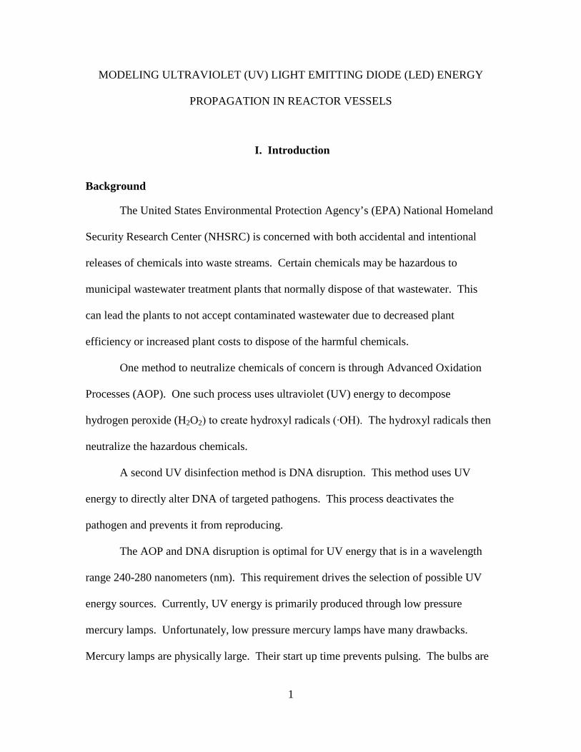
The United States Environmental Protection Agency’s (EPA) National Homeland

Security Research Center (NHSRC) is concerned with both accidental and intentional

releases of chemicals into waste streams. Certain chemicals may be hazardous to

municipal wastewater treatment plants that normally dispose of that wastewater. This

can lead the plants to not accept contaminated wastewater due to decreased plant

efficiency or increased plant costs to dispose of the harmful chemicals.

One method to neutralize chemicals of concern is through Advanced Oxidation

Processes (AOP). One such process uses ultraviolet (UV) energy to decompose

hydrogen peroxide (H2O2) to create hydroxyl radicals (∙OH). The hydroxyl radicals then

neutralize the hazardous chemicals.

A second UV disinfection method is DNA disruption. This method uses UV

energy to directly alter DNA of targeted pathogens. This process deactivates the

pathogen and prevents it from reproducing.

The AOP and DNA disruption is optimal for UV energy that is in a wavelength

range 240-280 nanometers (nm). This requirement drives the selection of possible UV

energy sources. Currently, UV energy is primarily produced through low pressure

mercury lamps. Unfortunately, low pressure mercury lamps have many drawbacks.

Mercury lamps are physically large. Their start up time prevents pulsing. The bulbs are

2

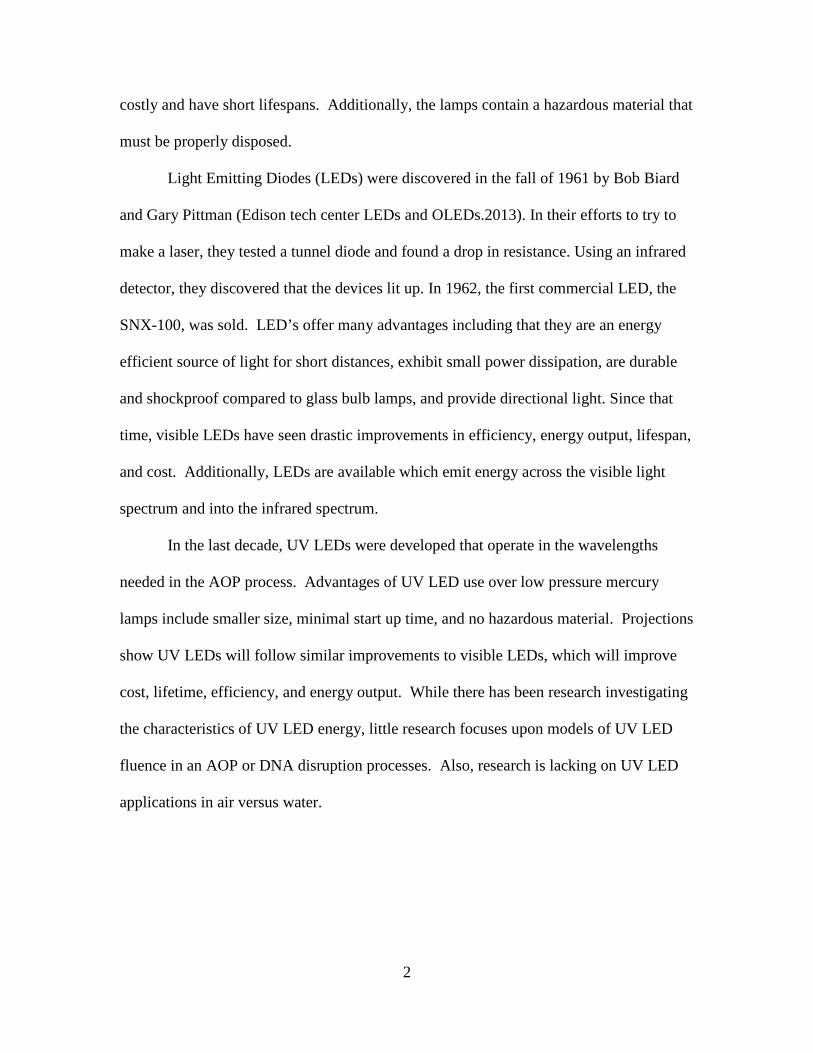
costly and have short lifespans. Additionally, the lamps contain a hazardous material that

must be properly disposed.

Light Emitting Diodes (LEDs) were discovered in the fall of 1961 by Bob Biard

and Gary Pittman (Edison tech center LEDs and OLEDs.2013). In their efforts to try to

make a laser, they tested a tunnel diode and found a drop in resistance. Using an infrared

detector, they discovered that the devices lit up. In 1962, the first commercial LED, the

SNX-100, was sold. LED’s offer many advantages including that they are an energy

efficient source of light for short distances, exhibit small power dissipation, are durable

and shockproof compared to glass bulb lamps, and provide directional light. Since that

time, visible LEDs have seen drastic improvements in efficiency, energy output, lifespan,

and cost. Additionally, LEDs are available which emit energy across the visible light

spectrum and into the infrared spectrum.

In the last decade, UV LEDs were developed that operate in the wavelengths

needed in the AOP process. Advantages of UV LED use over low pressure mercury

lamps include smaller size, minimal start up time, and no hazardous material. Projections

show UV LEDs will follow similar improvements to visible LEDs, which will improve

cost, lifetime, efficiency, and energy output. While there has been research investigating

the characteristics of UV LED energy, little research focuses upon models of UV LED

fluence in an AOP or DNA disruption processes. Also, research is lacking on UV LED

applications in air versus water.

3

Problem Statement

UV energy is historically used in mercury lamp applications to treat water.

Mercury lamps have multiple drawbacks that UV LEDs are able to solve. However, the

physical design and energy distribution between mercury lamps and LEDs are different.

A large amount of research exists on the design of energy distribution in mercury lamp

UV systems. UV LEDs, however, are relatively new in this application. Individual

characteristics of light and UV energy are well documented in literature. Despite this,

there is a knowledge gap of how these characteristics interact and how a single model can

describe the concentration of UV LED energy in a specific area.

This research effort focuses on modeling the characteristics of UV LED energy.

This effort will be useful to more efficiently design a device to apply a specified UV

dosage. Optimized vessel designs will lower operating costs and improve

disinfection/oxidation rates.

Research Objectives/Questions/Hypotheses

The objective of this research is to create and validate mathematical models of

energy propagation emitted by UV LEDs for the purpose of aiding in the design of AOP

or DNA disruption reactor vessels. The model will enable a detailed analysis of different

vessel designs to identify those which are optimal, and in turn identify which may be

most effective in neutralizing harmful pathogens. The research presented in this thesis

will answer the following research questions:

4

RQ1: What is an Advanced Oxidation Process (AOP) and DNA disruption?

How are they different and similar? Also, how are they used for water

disinfection?

RQ2: What sources of ultraviolet (UV) radiation have been used for the AOP

and DNA disruption in water disinfection applications?

RQ3: What are the measures of UV energy distribution in a reactor vessel?

RQ4: What mathematical models can be used to calculate the distribution and

absorption of UV Light Emitting Diode (LED) radiation as it propagates

through different mediums?

RQ5: What tools can be used to simulate these models to calculate the UV

energy present at any point within a UV reactor vessel?

RQ6: How do simulation results generated from the model compare to actual

experimental results collected from the laboratory?

RQ7: What UV LED reactor designs are most efficient for water disinfection?

Research Methodology

The research methodology used in this thesis is modeling and simulation. First,

the relevant UV and AOP literature is reviewed to identify governing equations. Second,

a model is synthesized at the appropriate level of abstraction to calculate the UV energy

present at any point within a reactor vessel based upon multiple factors including its

geometry, the location and intensity of the UV radiation sources, and the medium in

which the energy propagates. The model lacks an absorption coefficient for the

contaminant/microbes present in the solution and calculations for reflectance. Third, a

5

simulation tool suitable for modeling UV energy propagation within a reactor vessel is

selected and the relevant models of an actual UV reactor vessel are coded into the

simulation tool. Simulations are conducted and the results are compared to actual

measurements made in the laboratory. Finally, tradeoffs in the spacing of UV LEDs

within the vessel are discussed based upon the desired dosage and flow requirements.

Assumptions/Limitations

The models of UV radiation used in this thesis assume that the UV radiation

emitted by the sources is incoherent and that the impact of interference is negligible

compared to the loss due to absorption during propagation. The research is limited to

comparing the simulation results to actual laboratory measurements for only two different

reactor vessel geometries. This research effort represents the initial modeling effort to

understand UV energy propagation. There are factors which have been approximated in

an effort to simplify the model. These factors need more study to determine their impact

on the accuracy of the model.

Implications

The results from this research effort will provide a modeling and simulation

capability that will aid in the design and analysis of UV LED reactor vessels. UV LEDs

are still in their infancy and are projected to improve at rates similar to visible LEDs.

Optimized vessel design enables UV LEDs to be effective at an early stage and reduce

overall project costs. The variables within the model are easily altered to match new bulb

specifications and design new vessel shapes. The model may also be useful in

applications other than the AOP or DNA disruption. UV energy is also used in air

6

disinfection systems and multiple curing applications utilize UV energy in manufacturing

settings. Other industries may benefit from this research by optimizing energy

distribution and in turn reducing the power requirements and lowering system costs.

Preview

The next chapter, Chapter II, highlights the available literature on water

disinfection/oxidation, mercury lamp and LED bulb characteristics, and modeling

techniques for LED systems. Chapter III describes the methodology of forming the

MATLAB based model. Chapter IV reports and discusses the results. Finally, Chapter V

states the conclusions of this study and identifies areas for future research.

7

II. Literature Review

Chapter Overview

In this chapter, the primary methods of water disinfection along with the

advantages, disadvantages, and the major points on how the methods work are presented.

Next, the characteristics of UV mercury lamps and LED bulbs are discussed to provide

context for their application in UV reactor designs. A review of modeling techniques and

factors important in the design of water disinfection reactor vessels is then presented.

Finally, modeling and simulation environments are discussed.

Water Disinfection

Chlorine Disinfection

Chlorine disinfection has been the primary method to disinfect water for many

years in the United States. The process involves adding the optimal amount of chlorine

to a water source. However, chlorine disinfection has a few disadvantages. These

include introducing trihalomethane (THM) and haloacetic acid (HAA) as byproducts

(Taghipour & Sozzi, 2005). Additionally, two main harmful pathogens, Cryptosporidium

and Giardia, are chlorine resistant. Chlorine is also harmful to humans in high

concentrations and leaves an undesired smell and taste in disinfected water.

UV Disinfection

UV energy is defined as the energy spectrum between 100 and 400 nm. This

range is further broken down into VUV (vacuum UV), UVC, UVB, and UVA which

consist of wavelengths between 100-200, 200-280, 280-315, and 315-400 nm

respectively. The range 255-275 nm is proven to be the most effective range for DNA

8

destruction of harmful pathogens. This range is contained in the UVC range and is

slightly higher than the energy output for low pressure mercury lamps (254 nm). Figure

1 shows the electromagnetic spectrum with a callout for UV and visible energy (UVC

LED disinfection.2013; Wurtele et al., 2011).

Figure 1: Electromagnetic Spectrum (UVC LED disinfection.2013)

There are two main disinfection methods associated with ultraviolet (UV) energy.

The first utilizes the energy to directly deactivate the DNA of the pathogens, often called

DNA disruption. The second method uses the energy in an advanced oxidation process

(AOP) where the UV energy breaks down a chemical into radicals that neutralize the

harmful pathogens (UVC LED disinfection.2013).

Both of the UV methods are used in disinfection processes to overcome

disadvantages of chlorine systems. UV systems eliminate chlorine overdose issues and

pose no threat of overdosing since overexposure of UV energy is not harmful when

applied to water. UV disinfection systems reduce by-products and toxins introduced in

9

chlorine systems. Additionally, UV systems do not alter taste or smell of water (UVC

LED disinfection.2013).

Despite the numerous advantages of UV over chlorine disinfection systems, there

are a few disadvantages that affect UV systems. Sommer et. Al (2008) describe the

complexity of measuring and calculating UV energy. UV fluence cannot be directly

measured due to the intricacies of the system. Furthermore, UV lamp output, water flow,

ultraviolet transmittance (UVT), and hydraulic properties of the vessel are all factors that

complicate the system.

Lamps which output multiple wavelengths may increase the effectiveness of UV

disinfection. UV LEDs are able to do this to maximize germicidal effects by combining

bulb array patterns to create the right intensity and wavelength mix (C. Chatterley &

Linden, 2010). One study showed that combining UVC and UVA energy at 280/365 and

280/405 nm more effectively disinfected bacterial counts in urban wastewater effluent

than a single wavelength used alone (Chevremont, Farnet, Coulomb, & Boudenne, 2012;

Oguma, Kita, Sakai, Murakami, & Takizawa, 2013)

DNA Disruption

DNA disruption uses UV energy to alter the DNA of pathogens to inactivate the

targeted pathogen and prevent it from replicating (Figure 2). DNA disruption requires

specific UV doses to inactivate different pathogens. The pathogens Cryptosporidium and

Giardia are extremely resistant to chemicals such as chlorine, but correct doses of UV

energy can inactivate these harmful pathogens (UVC LED disinfection.2013).

10

Figure 2: UVC DNA Disruption (UVC LED disinfection.2013)

DNA inactivation in water occurs in the 240-280 nm electromagnetic range. The

most effective range for DNA UV absorption is known to be in the 260-265 nm range.

This is based on the most commonly targeted pathogens. The range may shift, however,

depending on the targeted pathogen. UV energy above and below this range still

demonstrate efficient inactivation, however wavelengths higher than the UVC range

required drastically higher dosages to achieve the same benefit (Bowker, Sain, Shatalov,

& Ducoste, 2011; Oguma et al., 2013; Wurtele et al., 2011).

Advanced Oxidation Process (AOP)

An Advanced Oxidation Process utilizes UV energy to oxidize the target

pathogens. AOP may also be used to oxidize chemicals of concern. This process

requires applying the correct dose of UV energy to a solution to reduce a chemical to

radicals that subsequently neutralize target pathogens. Chemicals are usually required to

be added to the system. Two of the most common oxidants used in AOP systems are

hydrogen peroxide (H2O2) and ozone (O3) (Legrini, Oliveros, & Braun, 1993).

11

Alpert, Knappe, and Ducoste describe the reactions involved in the AOP process

with hydrogen peroxide for the destruction of methylene blue. Their equations are all

single ordered, but reactions occur to reform hydrogen peroxide from the ∙OH radicals

and also multiple byproducts. This may result in a non-linear relationship between input

variables of UV energy, H2O2, and methylene blue and the resulting methylene blue

concentration. Increasing the ∙OH radical production may occur by using higher energy

and H2O2 concentrations (Alpert, Knappe, & Ducoste, 2010; Coenen et al., 2013).

Inactivation

Pathogen inactivation is measured by log reduction. Method of disinfection,

energy wavelength, pathogen type and intensity all factor into pathogen reduction. The

log reduction requirements are typically driven by regulations in order to protect human

health.

The US Environmental Protection Agency (EPA) regulates water disinfection in

the United States. The Surface Water Treatment Rule (SWTR), Interim Enhanced

Surface Water Treatment Rule (IESWTR), Long Term 1 Enhanced Surface Water

Treatment Rule (LT1ESWTR), and Long Term 2 Enhanced Surface Water Treatment

Rule (LT2ESWTR) are regulations set by the EPA. LT2ESWTR is currently being set in

place and is scheduled to be completed by 1 October 2014. A summary of the

regulations and their required log removal is shown in Table 1. Table 2 shows the EPA

UV dose requirements for Cryptosporidium, Giardia, and viruses. It is important to note

that the EPA report does not specify the wavelength used for the results in Table 2.

However, mercury lamps (254 nm) were the predominant technology used at the time of

publication in 2006 and are assumed to be used for this data. The relative dose suggests

12

that the 4 log reduction requirement for viruses may be the driving factor. This table

suggests that Cryptosporidium and Giardia reduction are more easily achieved than virus

reduction. Dose requirements may change with different applied wavelengths which may

make either the Cryptosporidium or Giardia requirement the driving factor.

Additionally, the results in Table 2 are based on DNA disruption and not an AOP system

(U.S. Environmental Protection Agency (EPA), 2006).

Table 1: Summary of Microbial and DBP Rules (U.S. Environmental Protection Agency (EPA), 2006)

Table 2: UV Dose Requirements (mJ/cm2) (U.S. Environmental Protection Agency (EPA), 2006)

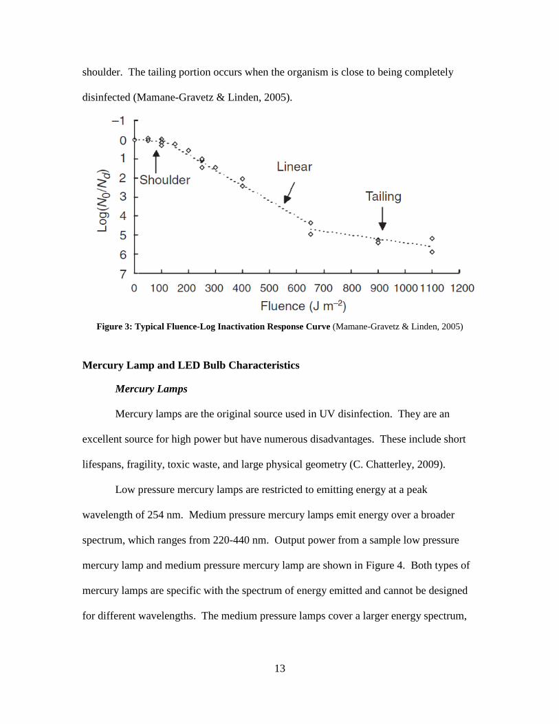
Mamane-Gravetz and Linden report that many organisms follow a shoulder, log-

linear, and tailing behavior at low, medium, and high fluence levels. This behavior is

portrayed in Figure 3 with Bacillus subtilis spores as the target organism. This behavior

is important due to the drastic increase in organism reduction after getting over the

13

shoulder. The tailing portion occurs when the organism is close to being completely

disinfected (Mamane-Gravetz & Linden, 2005).

Figure 3: Typical Fluence-Log Inactivation Response Curve (Mamane-Gravetz & Linden, 2005)

Mercury Lamp and LED Bulb Characteristics

Mercury Lamps

Mercury lamps are the original source used in UV disinfection. They are an

excellent source for high power but have numerous disadvantages. These include short

lifespans, fragility, toxic waste, and large physical geometry (C. Chatterley, 2009).

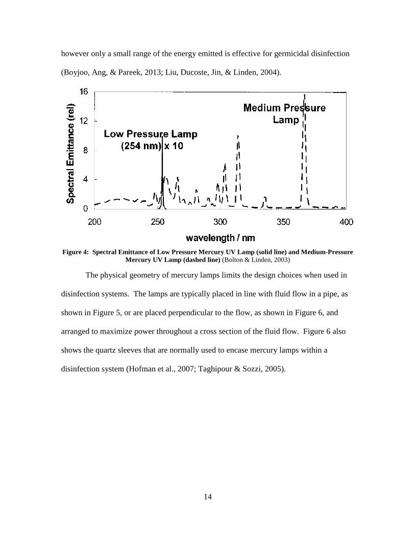
Low pressure mercury lamps are restricted to emitting energy at a peak

wavelength of 254 nm. Medium pressure mercury lamps emit energy over a broader

spectrum, which ranges from 220-440 nm. Output power from a sample low pressure

mercury lamp and medium pressure mercury lamp are shown in Figure 4. Both types of

mercury lamps are specific with the spectrum of energy emitted and cannot be designed

for different wavelengths. The medium pressure lamps cover a larger energy spectrum,

14

however only a small range of the energy emitted is effective for germicidal disinfection

(Boyjoo, Ang, & Pareek, 2013; Liu, Ducoste, Jin, & Linden, 2004).

Figure 4: Spectral Emittance of Low Pressure Mercury UV Lamp (solid line) and Medium-Pressure

Mercury UV Lamp (dashed line) (Bolton & Linden, 2003)

The physical geometry of mercury lamps limits the design choices when used in

disinfection systems. The lamps are typically placed in line with fluid flow in a pipe, as

shown in Figure 5, or are placed perpendicular to the flow, as shown in Figure 6, and

arranged to maximize power throughout a cross section of the fluid flow. Figure 6 also

shows the quartz sleeves that are normally used to encase mercury lamps within a

disinfection system (Hofman et al., 2007; Taghipour & Sozzi, 2005).

15

Figure 5: Mercury Lamp with Parallel Flow (Taghipour & Sozzi, 2005)

Figure 6: Mercury Lamp with Perpendicular Flow (Hofman et al., 2007)

UV LEDs

Studies are currently limited for UV LEDs and their application in either batch or

flow through designs. This is primarily due to the novelty of the technology and limited

16

power output of UV LED bulbs. UV LEDs are expected to see large improvements in

power, efficiency, and lifespan similar to the improvements seen in visible light LEDs in

the past two decades. UV LEDs already provide the benefits of a small form factor, no

toxic waste, and selectable wavelength over mercury lamps. Projections predict power,

efficiency, and lifespan to match or exceed mercury lamps in the near future. Shur and

Gaska predict UV LED applications will take off as performance of these bulbs increase

(C. Chatterley & Linden, 2010; Oguma et al., 2013; Shur & Gaska, 2010; Yu et al., 2013;

Yu, Achari, & Langford, 2013).

Efficiency

Low pressure mercury lamps are around 35-38% energy efficient. A 2010 study

by Shur and Gaska reveals that UV LEDs are currently less than 2% efficient, with 280

nm bulbs having the highest efficiency rate and efficiency decreasing at shorter

wavelengths. The internal efficiency of UV LEDs is between 15 and 70%; however,

internal absorption and internal reflection create a maximum of 2% wall plug efficiency.

The authors state that visible LEDs have resolved this problem and expect UV LEDs to

follow as shown in Figure 7. Visible LEDs currently exceed an efficiency of 75%, more

than twice the efficiency of mercury lamps (Bettles, Schujman, Smart, Liu, &

Schowalter, 2007; Shur & Gaska, 2010).

17

Figure 7: Achieved and Projected LED Performance (Shur & Gaska, 2010)

The efficiency growth rate is incredible for visible LEDs. Visible LEDs are the

most used type of LEDs on the market today. They are the most researched and have

significantly improved since the early 1990’s. Their efficiency has improved at an

average rate of 20 times per decade, which is due to advances in semiconductor and

packaging technology. There is a consensus among researchers that UV LEDs will

follow with similar success as visible LEDs, and the applications for UV LEDs will take

off with the improved technology (Bettles et al., 2007; C. Chatterley & Linden, 2010; Je

Wook Jang, Seung Yoon Choi, & Kon Son, 2011; Paisnik, Poppe, Rang, & Rang, 2012;

Shur & Gaska, 2010).

Lifespan

The lifespan of conventional lighting is often based on catastrophic failure.

Mature LEDs, on the other hand, are not prone to catastrophic failure and instead

18

progressively degrade over time. This changes the efficiency of the bulb and alters the

wavelength of the emitted energy (Je Wook Jang et al., 2011; Lenk & Lenk, 2011).

In visible light LEDs, yellowing of the lens, which is often formed from an epoxy,

changes the efficiency of the bulb and may also change the wavelength emitted. This

occurs from exposure to heat and light. As yellowing increases, LEDs have a

degradation effect that decreases light efficiency and changes the wavelength produced

by the bulb. Furthermore, UV wavelengths lead to a greater yellowing effect than visible

light when the same lens materials are applied. In addition to reduced transmission of the

optics, the LEDs may become less efficient due to charge trapping or other mechanisms

which affect the LEDs efficiency in converting electrons to photons. Multiple studies

show that thermal stress is the main cause of this type of LED degradation (Lenk & Lenk,

2011; Narendran, Gu, Freyssinier, Yu, & Deng, 2004; Paisnik et al., 2012; Tang et al.,

2012).

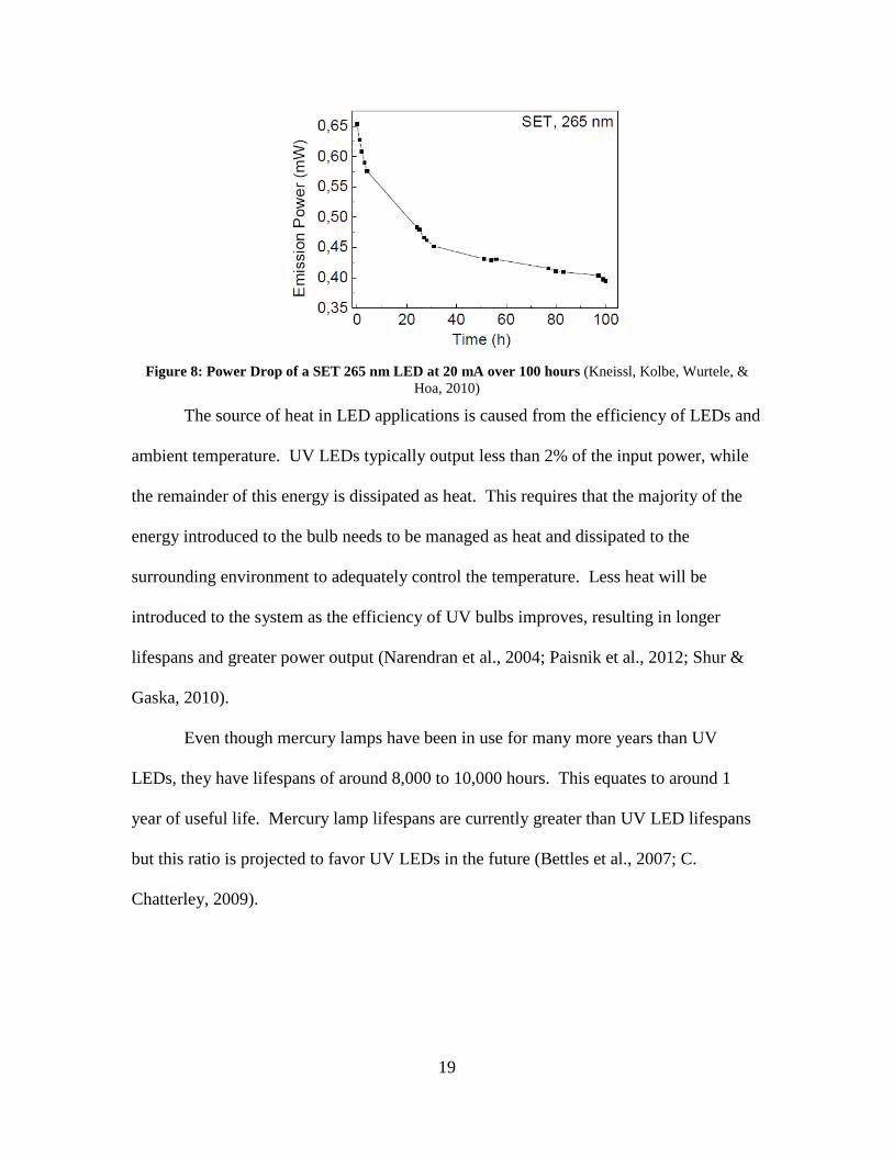
Since LEDs do not fail catastrophically, a common definition for LED failure is

based off of a specified drop in efficiency, which is normally a drop in the 30-50 percent

range. Some types of LEDs are able to be used up to 100,000 hours. However, studies

show that UV LEDs are currently limited to much shorter lifespans often less than 1,500

hours. These lifespans are also associated with a large drop in efficiency of around 40

percent after 100 hours of use followed by almost constant output power until the bulb is

no longer effective, shown in Figure 8 (Je Wook Jang et al., 2011; Wurtele et al., 2011).

19

Figure 8: Power Drop of a SET 265 nm LED at 20 mA over 100 hours (Kneissl, Kolbe, Wurtele, &

Hoa, 2010)

The source of heat in LED applications is caused from the efficiency of LEDs and

ambient temperature. UV LEDs typically output less than 2% of the input power, while

the remainder of this energy is dissipated as heat. This requires that the majority of the

energy introduced to the bulb needs to be managed as heat and dissipated to the

surrounding environment to adequately control the temperature. Less heat will be

introduced to the system as the efficiency of UV bulbs improves, resulting in longer

lifespans and greater power output (Narendran et al., 2004; Paisnik et al., 2012; Shur &

Gaska, 2010).

Even though mercury lamps have been in use for many more years than UV

LEDs, they have lifespans of around 8,000 to 10,000 hours. This equates to around 1

year of useful life. Mercury lamp lifespans are currently greater than UV LED lifespans

but this ratio is projected to favor UV LEDs in the future (Bettles et al., 2007; C.

Chatterley, 2009).

20

Wavelength

Studies show that about 265 nm UV energy has the maximum germicidal effect

for DNA disruption. Wavelengths of 365 nm require a much higher dose (on the order of

30,000 times) over 254 nm UV energy. Also the gap between 265 nm and 310 nm

energy corresponds to inactivation reduction of 6 orders of magnitude (C. Chatterley &

Linden, 2010).

One particular advantage to take note of is the ability of LEDs to produce a range

of wavelengths within the UV-C range while low pressure mercury lamps are restricted

to 254 nm. LEDs are typically considered to be a single wavelength, instead of

consisting of a spectrum of energy (Bettles et al., 2007; Wurtele et al., 2011).

Warm Up Time

Table 3 shows a sample of start-up and restart times for mercury lamps according

to tests from the EPA. Both low-pressure and medium-pressure mercury lamps require a

start-up time to reach full power. On the other hand, UV LEDs do not require a start-up

or restart time. They start at a higher power and decrease to their ‘maximum’ power over

10 minutes. Figure 9 shows a comparison of start-up power conducted by Chatterley.

The increased initial power of around 7% for UV LEDs may result in benefits of pulsing

the bulb (C. Chatterley, 2009; U.S. Environmental Protection Agency (EPA), 2006).

21

Table 3: Typical Start-up and Restart Times for Mercury Lamps1 (U.S. Environmental Protection Agency (EPA), 2006)

Figure 9: Warm-up Time for UV LEDs (■) Versus Low Pressure Lamps (▲) (C. Chatterley, 2009)

Pulsing

Pulsing light may decrease energy usage for a desired disinfection rate. A study

shows UVA-LEDs with a stable current at 0.5 amps utilizes more than 10 times the

energy of a 10 ms on to 100 ms off pulse rate for the same type bulb with a 1 amp current

22

for the same disinfection rate of E. coli in air. This research suggests that pulsing might

be beneficial due to the higher power used in the pulsed bulb than the steady state

experiment (Gadelmoula et al., 2009).

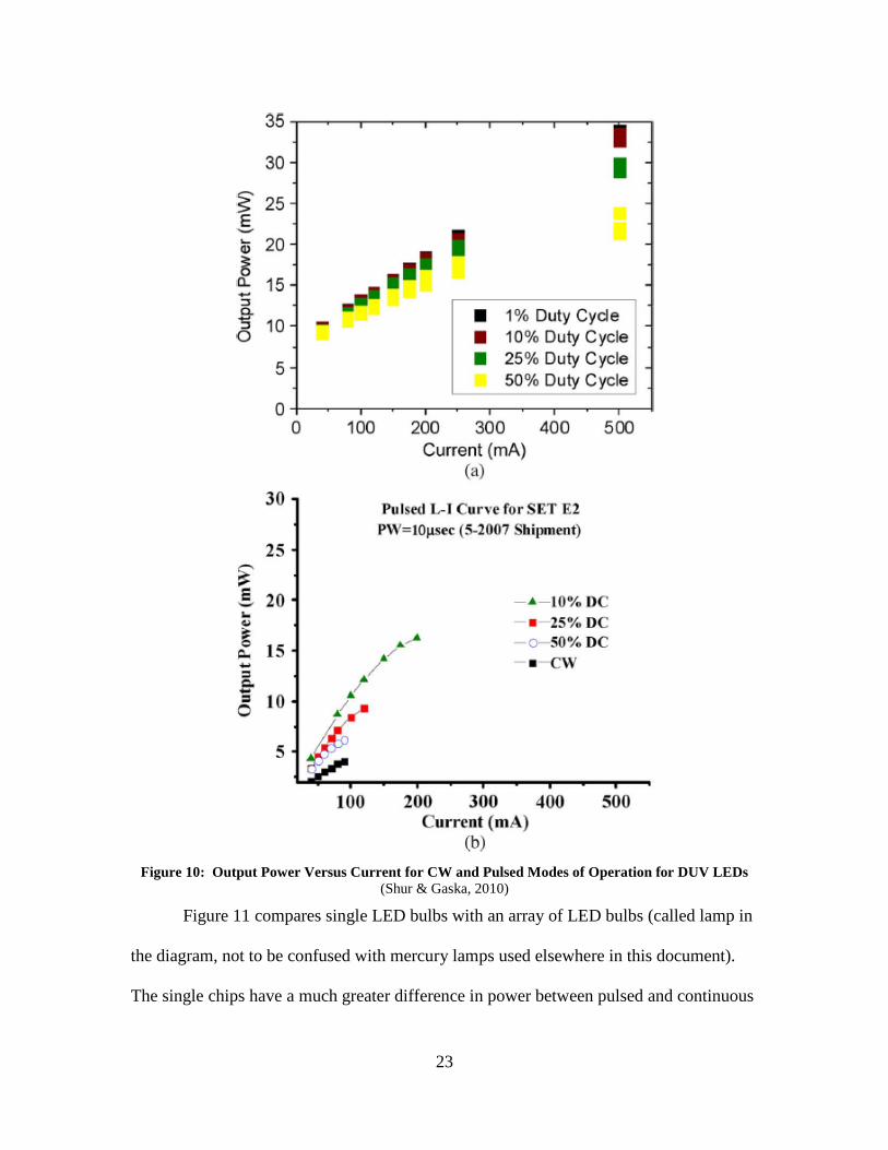
Shur and Gaska confirm that pulsing LEDs may provide higher power outputs

from the system. Figure 10 shows how a smaller pulsed duty cycle provides higher

power than larger duty cycles and continuous width (CW) operations. Pulsing LEDs

increases the output power by limiting heat generation within the LED package (Shur &

Gaska, 2010).

23

Figure 10: Output Power Versus Current for CW and Pulsed Modes of Operation for DUV LEDs

(Shur & Gaska, 2010)

Figure 11 compares single LED bulbs with an array of LED bulbs (called lamp in

the diagram, not to be confused with mercury lamps used elsewhere in this document).

The single chips have a much greater difference in power between pulsed and continuous

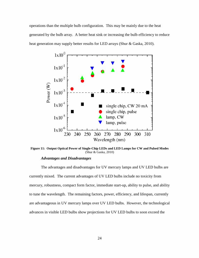
24

operations than the multiple bulb configuration. This may be mainly due to the heat

generated by the bulb array. A better heat sink or increasing the bulb efficiency to reduce

heat generation may supply better results for LED arrays (Shur & Gaska, 2010).

Figure 11: Output Optical Power of Single-Chip LEDs and LED Lamps for CW and Pulsed Modes

(Shur & Gaska, 2010)

Advantages and Disadvantages

The advantages and disadvantages for UV mercury lamps and UV LED bulbs are

currently mixed. The current advantages of UV LED bulbs include no toxicity from

mercury, robustness, compact form factor, immediate start-up, ability to pulse, and ability

to tune the wavelength. The remaining factors, power, efficiency, and lifespan, currently

are advantageous in UV mercury lamps over UV LED bulbs. However, the technological

advances in visible LED bulbs show projections for UV LED bulbs to soon exceed the

25

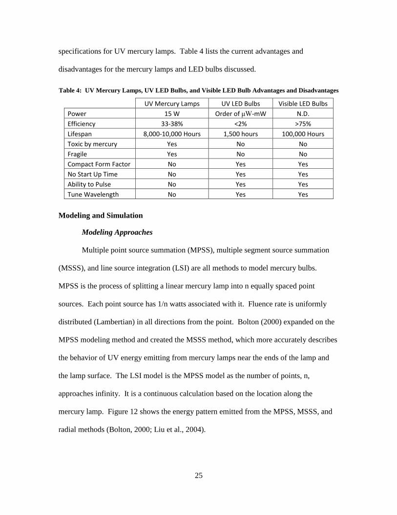
specifications for UV mercury lamps. Table 4 lists the current advantages and

disadvantages for the mercury lamps and LED bulbs discussed.

Table 4: UV Mercury Lamps, UV LED Bulbs, and Visible LED Bulb Advantages and Disadvantages

UV Mercury Lamps UV LED Bulbs Visible LED Bulbs Power 15 W Order of μW-mW N.D. Efficiency 33-38% <2% >75% Lifespan 8,000-10,000 Hours 1,500 hours 100,000 Hours Toxic by mercury Yes No No Fragile Yes No No Compact Form Factor No Yes Yes No Start Up Time No Yes Yes Ability to Pulse No Yes Yes Tune Wavelength No Yes Yes

Modeling and Simulation

Modeling Approaches

Multiple point source summation (MPSS), multiple segment source summation

(MSSS), and line source integration (LSI) are all methods to model mercury bulbs.

MPSS is the process of splitting a linear mercury lamp into n equally spaced point

sources. Each point source has 1/n watts associated with it. Fluence rate is uniformly

distributed (Lambertian) in all directions from the point. Bolton (2000) expanded on the

MPSS modeling method and created the MSSS method, which more accurately describes

the behavior of UV energy emitting from mercury lamps near the ends of the lamp and

the lamp surface. The LSI model is the MPSS model as the number of points, n,

approaches infinity. It is a continuous calculation based on the location along the

mercury lamp. Figure 12 shows the energy pattern emitted from the MPSS, MSSS, and

radial methods (Bolton, 2000; Liu et al., 2004).

26

Figure 12: MPSS, MSSS, and Radial Model Emittance Patterns (Liu et al., 2004)

Mercury lamps are often modeled using a Lambertian emittance pattern. A

Lambertian pattern is where emitted energy is constant independent of viewing angle

(Dereniak & Boreman, 1996). These energy sources are straightforward to model due to

limited changes in energy intensity. A good example is the incandescent light bulb. It

emits energy equally in all directions. Some mercury lamp models assume the lamp is an

infinite length and follow a Lambertian pattern. This radial method does not take into

account deviations at the ends of the lamp. The MPSS, MSSS, and LSI models help

solve this issue.

Design Factors

Crystal IS lists 3 important design factors to consider when choosing UV water

disinfection. They are water quality, water flow rate, and pathogen(s) to be inactivated.

Water quality determines the UV transmittance through the medium. Higher

transmittance produces better results. This is due to less turbidity, which absorbs less UV

energy. Water flow rate determines the exposure time, the lower the flow rate, the longer

the exposure which results in a greater log inactivation or requires higher lamp output.

Pathogens have different resistances to UV energy. The more resistant the pathogen the

27

more energy is required. AOP is dependent on reactions between the UV energy, oxidant

and target pathogens (UVC LED disinfection.2013).

Multiple Bulbs

Bulb layout is driven by the efficiency and uniformity requirements previously

discussed. The most efficient design requires a uniform energy array across the

disinfection interface. Additionally, the strength of the LEDs determines bulb spacing.

Higher output LEDs allow larger intervals between bulbs. Tighter spacing requirements

increases heat produced, which decreases energy efficiency. Altering the heat sink may

counter this effect for tightly spaced arrays (Wurtele et al., 2011).

Dose

The applied dose is the irradiance multiplied by exposure. There is currently no

method to directly measure contact time between an energy source and flowing water.

However, contact time is influenced by the flow rate and hydrodynamics, which can be

used to determine an approximate contact time (Wurtele et al., 2011).

Collimated Beam

Due to the low output power of UV LEDs, researchers often use a collimated

beam experiment to compare low and medium pressure mercury lamps to LED bulbs. In

this approach, multiple LED bulbs, sometimes on the order of 30, are placed in an array

to overlap the bulb’s fields of view to increase the irradiance. The goal of a collimated

beam is to produce parallel rays that form a uniform intensity over a given area.

However, the distribution of energy may prevent a uniform intensity. A uniform beam of

energy may be used to determine the log reduction associated with a given dose at

specific wavelengths (Blatchley III, 1997; Bolton, 2000; Bowker et al., 2011).

28

Modeling and Simulation Environments

Modeling and simulation is a method used to optimize designs prior to

manufacture. This method allows fewer device iterations, which, in turn reduces costs

associated with prototypes and experimentation. Multiple software platforms are

available for modeling and simulating physics based environments. Mathematica,

MATLAB, and COMSOL Multiphysics are three platforms that are suited for this use

(COMSOL multiphysics.2014; MATLAB - the language of technical computing.2014;

Wolfram mathematica 9.2014).

Each of these programs provides a suitable modeling and simulation environment.

They each have optional add-ons that aid in the modeling and simulation in domain

specific fields. Mathematica is built around programming in the mathematical domain.

It has many of the basics to start a theory based model. Similar to Mathematica,

COMSOL Multiphysics also offers a platform based in physical equations. One of the

main advantages of this program is the fluid modules. Arrays and matrices form the

framework for MATLAB. This program is designed to handle large quantities of data

and manipulate data through matrix operations. Each program offers two and three-

dimensional plots that aid in producing graphics to represent results created from the

program.

Chapter Summary

The advantages and disadvantages of chlorine disinfection, DNA disruption, and

the advanced oxidation process are introduced. UV disinfection offers many advantages

over chlorine disinfection technology. Next, the differences between mercury lamps and

29

LED bulbs are discussed. Finally, modeling approaches and factors are discussed. The

next chapter discusses the methodology used to model UV LEDs.

30

III. Methodology

Chapter Overview

In this chapter, the process used to conduct the research is presented. First, a

model of irradiance in a 3-dimensional space is introduced and discussed. The concepts

and equations necessary to conduct the research are identified and discussed. An

environment is selected as a vehicle to conduct the modeling and simulation of UV

reactor vessels. Finally, issues related to the modeling of UV energy propagation are

discussed.

Data Point Representation

When modeling a UV reactor vessel, it is necessary to identify all locations within

a three-dimensional space. For this research, data points are represented in both the

spherical and Cartesian coordinate systems. Data points are initialized in a local

spherical system which enables calculations based off of distance away from a point

source. The Cartesian coordinate system is then used to locate individual point sources in

an array and is required for generation of three dimensional plots.

The resolution of a model is directly affected by the number and spacing of the

initial data points. The greater number of data points in the needed range results in a

higher resolution for the model. The trade-off for higher resolution is longer computing

times or lack of computing memory to complete the operation.

31

Coordinate Systems

Use of both the Cartesian and spherical coordinate systems eases calculations. A

right hand Cartesian system is used and below shows the relationship between this

system and the spherical system used throughout this thesis. The azimuth is the angle in

the x-y plane that is measured counterclockwise starting on the x-axis. The elevation is

the angle measured from the x-y plane to the z axis. The spherical coordinate r is the

distance from the origin to the specified point.

Figure 13: Cartesian and Spherical Coordinate Systems

The equations necessary to convert between the coordinates are shown

below in equations 1 through 6.

32

Cartesian to Spherical

𝐫 = �𝐱𝟐 + 𝐲𝟐 + 𝐳𝟐 ( 1 ) Equation 1: Cartesian Coordinates to Spherical Coordinate 'r'

𝒂𝒛𝒊𝒎𝒖𝒕𝒉 = 𝒕𝒂𝒏−𝟏(𝒚𝒙) ( 2 )

Equation 2: Cartesian Coordinates to Spherical Coordinate ‘azimuth'

𝒆𝒍𝒆𝒗𝒂𝒕𝒊𝒐𝒏 = 𝒕𝒂𝒏−𝟏( 𝒛�𝒙𝟐+ 𝒚𝟐

) ( 3 )

Equation 3: Cartesian Coordinates to Spherical Coordinate 'elevation'

Spherical to Cartesian

𝒙 = 𝒓 ∗ 𝒄𝒐𝒔(𝒆𝒍𝒆𝒗𝒂𝒕𝒊𝒐𝒏) 𝒄𝒐𝒔(𝒂𝒛𝒊𝒎𝒖𝒕𝒉) ( 4 )

Equation 4: Spherical Coordinates to Cartesian Coordinate 'x'

𝒚 = 𝒓 ∗ 𝒄𝒐𝒔(𝒆𝒍𝒆𝒗𝒂𝒕𝒊𝒐𝒏) 𝒔𝒊𝒏(𝒂𝒛𝒊𝒎𝒖𝒕𝒉) ( 5 )

Equation 5: Spherical Coordinates to Cartesian Coordinate 'y'

𝒛 = 𝒓 ∗ 𝒔𝒊𝒏(𝒆𝒍𝒆𝒗𝒂𝒕𝒊𝒐𝒏) ( 6 )

Equation 6: Spherical Coordinates to Cartesian Coordinate 'z'

Modeling Concepts and Equations

Emission Angle

The emission angle of LEDs is used to describe energy propagation. This angle is

used to describe the intensity of energy associated at a specific angle from the center of

the energy transmission. The emission angle is also used to calculate area, later used to

determine irradiance.

The emission angle of LEDs restricts the bulbs from projecting a Lambertian

energy pattern. These bulbs differ from a Lambertian source in two ways. The first

difference is that the energy pattern is restricted to a conical pattern. The second

33

difference is the intensity is dependent on the angle from the center of the beam. Most

manufacturers publish data on the energy pattern emitted by their products. The

specification sheets normally report the emittance pattern through air. A conversion is

needed to determine the emission angle of a LED bulb in a medium other than air.

Snell’s law, shown in Equation 7, calculates the refracted angle when energy enters a new

medium (Halliday, Resnick, & Walker, 2005).

𝒏𝟏 𝐬𝐢𝐧 𝜽𝟏 = 𝒏𝟐 𝐬𝐢𝐧𝜽𝟐 ( 7 ) Equation 7: Snell's Law

The variables on the left hand side of the equation describe the LED bulb and the

variables on the right hand side describe the characteristics of air when applied to the

LED bulb and air interface. The index of refraction, n, is readily available for air and the

manufacturer provides the emission angle in air. The index of refraction and internal

angle of energy within the LED is not known, but the left hand side of the equation may

be represented by a constant since these values do not change when introducing a new

medium. This transforms Equation 7 into Equation 8, and can be reduced to Equation 9.

𝒏𝒃𝒖𝒍𝒃 𝐬𝐢𝐧 𝜽𝒃𝒖𝒍𝒃 = 𝒏𝒎𝒆𝒅𝒊𝒖𝒎 𝐬𝐢𝐧 𝜽𝒎𝒆𝒅𝒊𝒖𝒎 ( 8 ) Equation 8: Snell's Law with LED and Medium Identified

𝑪𝒐𝒏𝒔𝒕𝒂𝒏𝒕𝑳𝑬𝑫 = 𝒏𝒎𝒆𝒅𝒊𝒖𝒎 𝐬𝐢𝐧𝜽𝒎𝒆𝒅𝒊𝒖𝒎 ( 9 ) Equation 9: Snell's Law with LED Constant and Medium Identified

Equation 9 can be solved for ConstantLED and now be applied to a new medium to

determine the emission angle in a medium other than that specified by the manufacturer.

34

Intensity

Intensity is measured in watts emitted from a light source per steradian.

Steradians are a measurement of solid angle where a complete sphere contains 4π

steradians. Equation 10 calculates the solid angle, steradians, from the surface area of a

sphere contained from the angle and the radius of the sphere. The units of area and radius

must cancel (Dereniak & Boreman, 1996).

𝝎 = 𝑨𝒓𝟐

( 10 )

Equation 10: Solid Angle

Where:

ω = solid angle [steradians]

A = contained surface area of sphere

r = radius of sphere

Equation 11 aides in determining the surface area of a sphere and is represented in

Figure 14 (Lindeburg, 2011).

𝑨 = 𝟐𝝅𝒓𝟐(𝟏 − 𝐜𝐨𝐬 𝜽𝟎) ( 11 ) Equation 11: Surface Area of Sphere Contained by Specified Solid Angle

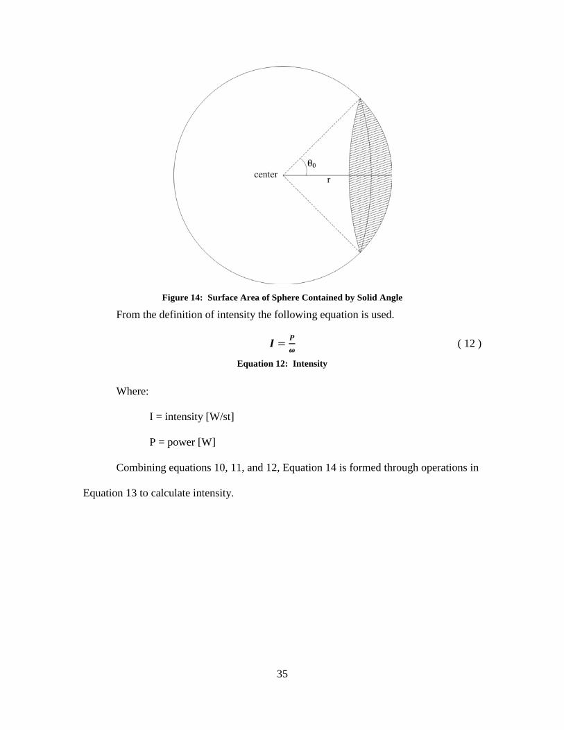
35

Figure 14: Surface Area of Sphere Contained by Solid Angle

From the definition of intensity the following equation is used.

𝑰 = 𝑷𝝎

( 12 )

Equation 12: Intensity

Where:

I = intensity [W/st]

P = power [W]

Combining equations 10, 11, and 12, Equation 14 is formed through operations in

Equation 13 to calculate intensity.

36

𝑰 = 𝑷𝝎

= 𝑷𝑨𝒓𝟐�

= 𝑷𝟐𝝅𝒓𝟐(𝟏−𝐜𝐨𝐬𝜽𝟎)

𝒓𝟐�

= 𝑷𝟐𝝅(𝟏−𝐜𝐨𝐬 𝜽𝟎)

( 13 )

Equation 13: Converting Intensity Equation to Limited Solid Angle

𝑰 = 𝑷𝟐𝝅(𝟏−𝐜𝐨𝐬𝜽𝟎)

( 14 )

Equation 14: Intensity Limited to Solid Angle

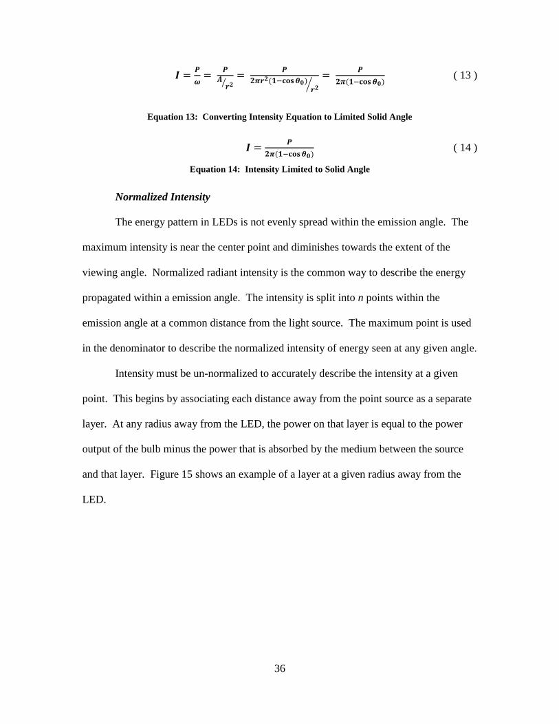
Normalized Intensity

The energy pattern in LEDs is not evenly spread within the emission angle. The

maximum intensity is near the center point and diminishes towards the extent of the

viewing angle. Normalized radiant intensity is the common way to describe the energy

propagated within a emission angle. The intensity is split into n points within the

emission angle at a common distance from the light source. The maximum point is used

in the denominator to describe the normalized intensity of energy seen at any given angle.

Intensity must be un-normalized to accurately describe the intensity at a given

point. This begins by associating each distance away from the point source as a separate

layer. At any radius away from the LED, the power on that layer is equal to the power

output of the bulb minus the power that is absorbed by the medium between the source

and that layer. Figure 15 shows an example of a layer at a given radius away from the

LED.

37

Figure 15: Spherical Cap with Elevation Rings and Points

Each layer is segmented into rings that represent elevations away from the LED’s

centerline. Each ring is divided into a specific number of segments represented by a

point in the center of that segment. Increasing the number of rings and points on each

ring increases the accuracy of the model.

Each ring is evenly spaced between the centerline and the extent of the emission

angle. Rings are measured by an elevation angle away from the centerline. The

manufacturer’s specifications are used to fit a line to their data to determine the

38

normalized intensity at any given location on a layer based on the angle from the

centerline.

Next, the sum of normalized intensity by all the points on one layer is calculated.

Then the normalized intensity at each point on the layer is divided by the sum of

normalized intensity on the layer to determine the percent intensity at each point on the

layer. Finally, the percent intensity at each point is multiplied by the intensity on the

layer to determine the intensity at each point. This process is shown in equations 15

through 17.

∑𝒏𝒐𝒓𝒎𝒂𝒍𝒊𝒛𝒆𝒅𝒊𝒏𝒕𝒆𝒏𝒔𝒊𝒕𝒚𝒍𝒂𝒚𝒆𝒓 = ∑𝒏𝒐𝒓𝒎𝒂𝒍𝒊𝒛𝒆𝒅𝒊𝒏𝒕𝒆𝒏𝒔𝒊𝒕𝒚𝒑𝒐𝒊𝒏𝒕𝒔 𝒐𝒏 𝒍𝒂𝒚𝒆𝒓 ( 15 ) Equation 15: Sum Normalized Intensity on Layer

%𝒊𝒏𝒕𝒆𝒏𝒔𝒊𝒕𝒚𝒑𝒐𝒊𝒏𝒕 = 𝒏𝒐𝒓𝒎𝒂𝒍𝒊𝒛𝒆𝒅𝒊𝒏𝒕𝒆𝒏𝒔𝒊𝒕𝒚𝒑𝒐𝒊𝒏𝒕∑𝒏𝒐𝒓𝒎𝒂𝒍𝒊𝒛𝒆𝒅𝒊𝒏𝒕𝒆𝒏𝒔𝒊𝒕𝒚𝒍𝒂𝒚𝒆𝒓

( 16 )

Equation 16: Percent Intensity at Each Point

𝒊𝒏𝒕𝒆𝒏𝒔𝒊𝒕𝒚𝒑𝒐𝒊𝒏𝒕 = %𝒊𝒏𝒕𝒆𝒏𝒔𝒊𝒕𝒚𝒑𝒐𝒊𝒏𝒕 ∗ 𝒊𝒏𝒕𝒆𝒏𝒔𝒊𝒕𝒚𝒍𝒂𝒚𝒆𝒓 ( 17 ) Equation 17: Intensity at Each Point

Irradiance

Irradiance (E) of light is the intensity that is emitted on a surface. For a

Lambertian source, irradiance is calculated based off of the intensity of energy and

distance from the light source. The irradiance decreases exponentially with distance, as

seen in Equation 18. Milliwatts per square centimeter are typical units for irradiance in

ultraviolet LED applications (Bolton, 2000; Dereniak & Boreman, 1996).

𝑬 = 𝑰 𝒓𝟐� ( 18 )

Equation 18: Irradiance

Where:

39

E = Irradiance [W/m2]

I = Intensity [W/ω]

r = distance [m]

This equation is useful with mercury lamps. Equation 18 above is converted into

Equation 19 below. In this equation, intensity is reduced to power and 4π is placed in the

denominator, representing the number of steradians in a complete sphere. This allows a

user to directly input the typical specification, Watts, directly from the manufacturer’s

specification sheet for a mercury lamp (Bowker et al., 2011; Dereniak & Boreman,

1996).

𝑬 = 𝑷𝟒𝝅𝒓𝟐

( 19 )

Equation 19: Mercury Lamp Irradiance

A rough estimation of LED bulbs is based off of Equation 19 above. Equation 20

accounts for the limited angle that is projected from an LED source. This assumes

Lambertian properties within the emission angle of the LED and equally distributes the

power in that area (Bowker et al., 2011).

𝑬 = 𝑷𝟐𝝅𝒓𝟐(𝟏−𝐜𝐨𝐬(𝜃0))

( 20 )

Equation 20: LED Bulb Irradiance

These equations are firmly based on power per square area. Since an LED is not

a Lambertian source and the energy propagated from an LED is not uniformly

distributed, these equations do not accurately describe the energy density at specific

points for a non-Lambertian energy spread. The correct approach is to determine the

irradiance associated with each point. This process involves calculating the intensity

40

throughout the volume to be modeled and the area associated with that volume. Dividing

the intensity at a point by the area at that point results in irradiance at that point.

Absorption

The Beer-Lambert law describes absorption through a medium. The law states

that absorption is constant through a uniform material and can be calculated with an

absorption constant and the path length. Equations 21 and 22 show how absorption

affects irradiance (Liu et al., 2004; Beer's law.).

𝑬 = 𝑬𝟎𝑼 ( 21 ) Equation 21: Beer-Lambert Law

Where:

E0 = irradiance without absorption

U = absorption attenuation factor

𝑼 = 𝒆−𝒂(𝝀)𝒍 ( 22 ) Equation 22: Absorption Attenuation Factor

Where:

a(λ) = absorption coefficient at a specific wavelength [1/m]

l = path length [m]

The absorption factor may be applied before or after distributing the intensity

across all points on a layer. Doing this after un-normalizing the intensity allows the

model to use the same intensity across the area covered by each layer.

Spherical to Cartesian Coordinates

At this point the coordinates need to be converted from spherical to Cartesian

coordinates. Local spherical coordinates up to this point enable the energy to be evenly

41

distributed and solved at numerous steps away from the bulb. However, three

dimensional plots often require evenly spaced Cartesian coordinates.

Since the data points are originally set up in spherical coordinates, the Cartesian

coordinates are not evenly spaced. The un-spaced Cartesian coordinates are rounded to

the nearest evenly spaced grid location to allow graphing volume data. Moving these

points reduces the accuracy of the model, but decreasing the step size between points

reduces this effect.

After the Cartesian coordinates are moved, they must be arranged into increasing

coordinate value since they are still ordered based off of the original spherical

coordinates. Another operation is performed to move the points into the correct

sequence.

Bulb Array

After the coordinate system is converted from spherical to Cartesian coordinates,

the bulb array is arranged. UV energy is additive and a simple point source summation

can detail the energy pattern emitted on a surface or in a volume. The LED bulb model is

reproduced for each LED in the array and offset from the center of the vessel to place the

LEDs in the correct locations (Blatchley III, 1997; Bolton, 2000; Bowker et al., 2011).

Limit Bulb Array

The bulb array matrix is now limited to the vessel dimensions. The irradiance

matrix is set to zero for points that fall outside the extents of the vessel size. The array is

also limited to the fluid height for batch experiments that do not fill the vessel.

42

Pathogen Inactivation

Pathogen inactivation is calculated based off of the log reduction in a solution.

This is reported as a log reduction, calculated by Equation 23. The initial and final

concentrations are needed to determine the pathogen inactivation in a solution. Empirical

methods are often used to determine the dose associated with the log reduction. UV dose

is the summation of the integral of UV irradiance with respect to time (Wurtele et al.,

2011).

𝒍𝒐𝒈𝑹𝒆𝒅𝒖𝒄𝒕𝒊𝒐𝒏 = 𝒍𝒐𝒈 (𝒄𝒐𝒏𝒄𝒆𝒏𝒕𝒓𝒂𝒕𝒊𝒐𝒏𝑰𝒏𝒊𝒕𝒊𝒂𝒍𝒄𝒐𝒏𝒄𝒆𝒏𝒕𝒓𝒂𝒕𝒊𝒐𝒏𝑵𝒆𝒘

) ( 23 )

Equation 23: Log Reduction

DNA disruption and AOP dose to log inactivation calculations differ. DNA

disruption follows the shoulder, log-linear, and tailing regions introduced in Chapter II.

DNA repair occurs in the shoulder region. The log reduction rate is slower in this region

than the log-linear region. The log-linear region has the greatest contaminant reduction

associated with it. The tailing region follows this region. The contaminant reduction rate

slows in this region due to the sparse number of contaminants. The EPA reports the dose

summation is valid for DNA disruption in the range of 1-200 mW/cm2. UV dose is not

affected by long exposure over a smaller irradiance or shorter exposure over a longer

irradiance in this range. This range corresponds to the log-linear region (Mamane-

Gravetz & Linden, 2005; U.S. Environmental Protection Agency (EPA), 2006).

AOPs do not follow the shoulder, log-linear, and tailing regions. Multiple

equations govern the creation of radicals during UV irradiation. The radicals either

neutralize the target pathogen, reform to the original oxidant, or react to form byproducts

(Alpert et al., 2010; Coenen et al., 2013).

43

The process for batch and flow experiments is to first calculate the UV dose at

each point. The second step is to calculate the log inactivation at each point. This

calculation is conducted by fitting a line to data obtained to show the relationship

between concentration reduction and dose. Next, the new concentration is calculated at

each point. A mixing rate is introduced to this process to account for stirring that occurs

in batch experiments. Assumptions must be made for flow experiments regarding fluid

flow.

MATLAB

The governing equations used in this research were coded into MATLAB. The

main advantage this program offers over the other possible choices is the ability to

compute large matrices. This is required to set up a suitable three-dimensional coordinate

space so that the irradiance could be calculated for each point in the system. MATLAB

also has robust graphics capabilities that allow visualization of this data. The program is

relatively easy to program, with built in functions and the ability to easily code additional

functions. Finally, MATLAB is readily available in the research environment.

Graphing in MATLAB

Graphing in MATLAB requires an evenly spaced three dimensional grid and

corresponding matrix with volume data. The grid size needs to be large enough to cover

the irradiated area and the vessel volume. The grid needs to be capable of covering a

large area if the design calls for multiple bulbs. Three dimensional graphs are used to

show the overall irradiance effect in the vessel.

44

Reactor Vessel Optimization

Optimum reactor vessel geometry is dependent on output power and shape of

energy propagation. The goal is to maximize the log-linear region in the reactor. The

optimum size of the reactor is driven by the output power and the bulb array. The

required log reduction and dose to reduction rate drive the flow rate, or duration for batch

experiments.

Chapter Summary

In this chapter, the information required to understand how to duplicate the

research effort was presented. The governing principles and concepts of UV energy

propagation were identified, key equations used in the modeling activity were selected,

and an environment suitable for implementing and simulating the models was selected.

In the next chapter, the results of the application of the research methodology are

presented.

45

IV. Data and Results

Chapter Overview

In this chapter, the research methodology presented in Chapter III is applied to

model and simulate the UV energy distribution in two different UV reactor vessel

designs. The results from the simulation are analyzed and compared to experimental

results collected from a real-world experiment. Strengths and weaknesses of the modeling

and simulation effort in terms of accuracy and efficiency are identified. The referenced

MATLAB model throughout this chapter is located in the Appendix.

Baseline

The baseline for the model was based upon a UV reactor vessel and LED array

created by Spencer (Spencer, 2014). This vessel was used for both batch and flow

through experiments using Bacillus globigii (formerly known as Bacillus subtilis var.

niger) spores and methylene blue (indicator dye), respectively. The batch experiments

disinfected the water (inactivated spores via DNA disruption) while the flow through

experiments used an AOP process with hydrogen peroxide to generate hydroxyl radicals.

The vessel had an interior diameter of 2.87 inches with a depth of 3 inches and was made

of polished stainless steel (Figure 16).

46

Figure 16: Vessel

The bulb array consisted of 7 LEDs configured in an array on the bottom plate of

the vessel. One bulb was centered with the remaining 6 bulbs placed equally along a 1

inch (2.54 cm) radius from the center. The physical dimensions of the LED array are

shown in Figure 17. Once configured, the bottom and top plates were bolted to the

bottom and top of the vessel.

47

Figure 17: LED Plate with LED Spacing

The vessel was designed using the English coordinate system. However, the

metric system is used throughout this document. The Cartesian system is initialized with

the (x, y) reference with the zero coordinate set at the center bulb. The following table

shows the bulb spacing in both English and in the International System of Units (SI)

metric units.

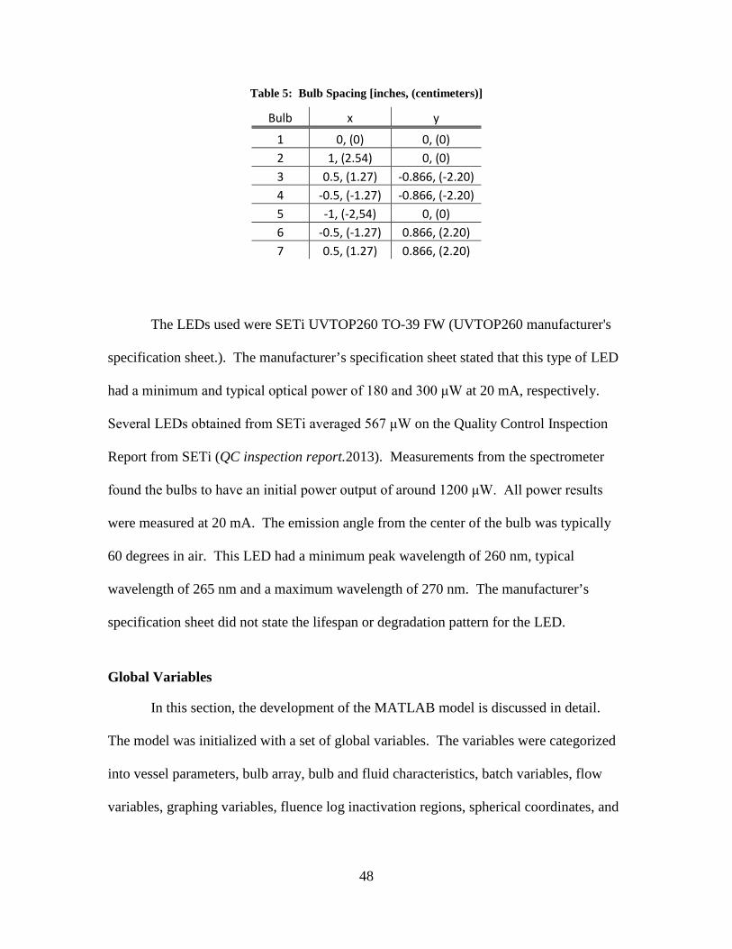
48

Table 5: Bulb Spacing [inches, (centimeters)]

Bulb x y

1 0, (0) 0, (0) 2 1, (2.54) 0, (0) 3 0.5, (1.27) -0.866, (-2.20) 4 -0.5, (-1.27) -0.866, (-2.20) 5 -1, (-2,54) 0, (0) 6 -0.5, (-1.27) 0.866, (2.20) 7 0.5, (1.27) 0.866, (2.20)

The LEDs used were SETi UVTOP260 TO-39 FW (UVTOP260 manufacturer's

specification sheet.). The manufacturer’s specification sheet stated that this type of LED

had a minimum and typical optical power of 180 and 300 μW at 20 mA, respectively.

Several LEDs obtained from SETi averaged 567 μW on the Quality Control Inspection

Report from SETi (QC inspection report.2013). Measurements from the spectrometer

found the bulbs to have an initial power output of around 1200 μW. All power results

were measured at 20 mA. The emission angle from the center of the bulb was typically

60 degrees in air. This LED had a minimum peak wavelength of 260 nm, typical

wavelength of 265 nm and a maximum wavelength of 270 nm. The manufacturer’s

specification sheet did not state the lifespan or degradation pattern for the LED.

Global Variables

In this section, the development of the MATLAB model is discussed in detail.

The model was initialized with a set of global variables. The variables were categorized

into vessel parameters, bulb array, bulb and fluid characteristics, batch variables, flow

variables, graphing variables, fluence log inactivation regions, spherical coordinates, and

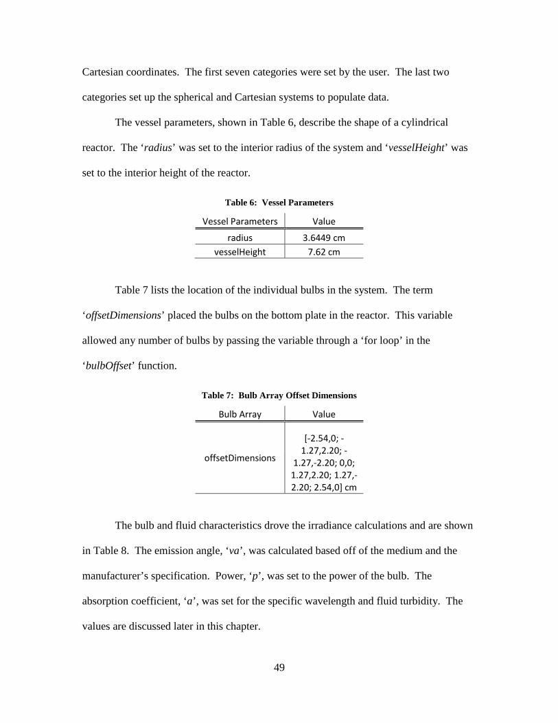
49

Cartesian coordinates. The first seven categories were set by the user. The last two

categories set up the spherical and Cartesian systems to populate data.

The vessel parameters, shown in Table 6, describe the shape of a cylindrical

reactor. The ‘radius’ was set to the interior radius of the system and ‘vesselHeight’ was

set to the interior height of the reactor.

Table 6: Vessel Parameters

Vessel Parameters Value

radius 3.6449 cm vesselHeight 7.62 cm

Table 7 lists the location of the individual bulbs in the system. The term

‘offsetDimensions’ placed the bulbs on the bottom plate in the reactor. This variable

allowed any number of bulbs by passing the variable through a ‘for loop’ in the

‘bulbOffset’ function.

Table 7: Bulb Array Offset Dimensions

Bulb Array Value

offsetDimensions

[-2.54,0; -1.27,2.20; -

1.27,-2.20; 0,0; 1.27,2.20; 1.27,-2.20; 2.54,0] cm

The bulb and fluid characteristics drove the irradiance calculations and are shown

in Table 8. The emission angle, ‘va’, was calculated based off of the medium and the

manufacturer’s specification. Power, ‘p’, was set to the power of the bulb. The

absorption coefficient, ‘a’, was set for the specific wavelength and fluid turbidity. The

values are discussed later in this chapter.

50

Table 8: Bulb and Fluid Characteristics

Bulb and Fluid Characteristics Value

va 39.72 degrees

p 180, 300, 567, or 1200 μW

a .01 cm-1

The batch variables, shown in Table 9, are specific to a previous experiment

(Tran, 2014). The initial concentration, ‘concentrationInitial’, was the same for each of

the batch trials. The experiment time, ‘time’, was set for one of the two experiment

durations. Mix time, ‘mixTime’, was set from 1 to the duration with intervals every five

seconds. The fluid height, ‘fluidHeightBatch’, was set to the distance that encases 100 ml

of solution.

Table 9: Batch Variables

Batch Variables Value

concentrationInitial 7x106 cfu/ml

time 64 or 129 seconds

mixTime 1 to time fluidHeightBatch 2.396 cm

Similar to the batch variables, the flow variables, shown in Table 10, were

specific to a separate recent experiment (Duckworth, 2014) experiments. The flow rate,

‘flowRate’, was set by default to 1.4 mL/min. The fluid height, ‘fluidHeightFlow’, was

set to the vessel height to account for a full reactor (7.62 cm).

51

Table 10: Flow Variables

Flow Variables Value

flowRate 1.4 mL/min fluidHeightFlow 7.62 cm

Table 11 shows the graphing variables, which allowed the user to specify a space

that encompasses the reactor and change the step size. The step size increased and

decreased the space between the data points which affected the resolution of the model.

Table 11: Graphing Variables

Graphing Variables Value

stepSize 0.1 cm xGridMin -10 cm xGridMax 10 cm yGridMin -10 cm yGridMax 10 cm zGridMin 0 cm zGridMax 10 cm

The fluence log inactivation variables, shown in Table 12, allowed for

calculations and graphs for each of the regions. The log linear and tailing minimums are

not stated since they are equal to the shoulder and log linear regions, respectively.

Table 12: Fluence Log Inactivation Regions

Fluence Log Inactivation

Regions Value

shoulderMin 100 μW/cm2 shoulderMax 1,000 μW/cm2

logLinearMax 200,000 μW/cm2

tailingMax 1,000,000 μW/cm2

52

Two coordinate systems were also initialized. The first was a localized spherical

system used for individual LED bulbs, shown in Table 13. This required values for

azimuth, elevation, and r. The ‘linspace’ command was used to set equally spaced values

between a minimum and maximum value. The number of points could be set to the

default of 100 or the points could be increased or decreased to produce the desired

resolution/model run time trade off. Azimuth is set to -179 to 180 degrees with 360

steps. Elevation was set to provide the points between the emission angle and the center

of the beam with 100 steps. Since MATLAB’s spherical system measured elevation from

the x-y axis up to the z axis and the center of the beam was considered zero emission

angle, (90 – emission angle) was set for the minimum value and 90 was set to the

maximum value. The term ‘r’ was set to cover the needed distance. This was determined

by the vessel geometry to ensure irradiance is calculated for every point within the vessel.

In this case, ‘r’ was set from 0.1 to 10 cm with 100 steps. This covered the distance from

the LED plate to the opposite side of the vessel for the entire emission angle. This

dimension did not start at zero to avoid division of zero in the irradiance calculations.

Table 13: Spherical Coordinates

Spherical Coordinates

azInitial -179 to 180 degrees, 360 steps elInitial va to 90 degrees, 100 steps rInitial 0.1 to 10 cm, 100 steps

az azimuth array of 3D spherical space el elevation array of 3D spherical space r radius array of 3D spherical space

The second coordinate system was a global Cartesian system, shown in Table 14.

This system consisted of x, y, and z coordinates that represented the three dimensional

53

space of the vessel in .1 cm increments. An evenly spaced Cartesian coordinate system

was required to graph volume data in MATLAB.

Table 14: Cartesian Coordinates

Cartesian Coordinates

x1 -10 to 10 cm, 201 steps y1 -10 to 10 cm, 201 steps z1 0 to 10 cm, 101 steps

xGraph x array of 3D Cartesian space yGraph y array of 3D Cartesian space zGraph z array of 3D Cartesian space

The data points for each coordinate system were combined to form a matrix for

the azimuth, elevation, and r and x, y, and z for the spherical and Cartesian coordinate

systems respectively. This was completed using MATLAB’s ‘meshgrid’ function.

Calculations were based off of this initial spherical matrix to determine irradiance at all

of the points within the matrix. The initial Cartesian matrix was used to plot results.

Emission Angle

The SETi specification sheet for their flat window bulb stated that the emission

angle, angle between the center of the energy propagation and extents, in air was

typically 60 degrees. They also gave their typical angular diagram, which is displayed in

Figure 18. The power/radiant intensity was the expected normalized value by the

manufacturer and is further discussed in the next two sections.

54

Figure 18: Typical Angular Diagram, Air

Table 15 lists the minimum, maximum, and calculates the average value for each

angle reported by the manufacturer.

Table 15: Normalized Radiant Intensity Minimum, Maximum, and Averaged

Angle (Degrees)

Radiant Intensity Minimum

Radiant Intensity

Maximum

Radiant Intensity Average

0 0.96 0.96 0.96 10 0.98 1 0.99 20 0.96 0.98 0.97 30 0.88 0.99 0.935 40 0.78 0.94 0.86 50 0.68 0.72 0.7 60 0.44 0.49 0.465 70 0 0.34 0.17

The averaged radiant intensity was plotted against the emission angle to depict the

expected intensity from a SETi flat window LED bulb in air, shown in Figure 19.

55

Figure 19: Averaged Angular Diagram, Air

Snell’s law was used to calculate the emission angle and shift the power/radiant

intensity ratio from air to the correct angle for water. This was done by rearranging and

substituting the mediums into Equation 9, from Chapter III, to obtain Equation 24.

𝜽𝒘𝒂𝒕𝒆𝒓 = 𝐬𝐢𝐧−𝟏( 𝒏𝒂𝒊𝒓𝒏𝒘𝒂𝒕𝒆𝒓

𝐬𝐢𝐧 𝜽𝒂𝒊𝒓) ( 24 )

Equation 24: Snell's Law Rearranged for Water Angle

The values for the index of refraction for air and water were 1.0002967 and

1.3556, respectively, at 270 nm (Polyanskiy, 2013). Solving for the typical emission

angle for SETi flat window bulbs, the emission angle was 39.72° in water.

𝜽𝒘𝒂𝒕𝒆𝒓 = 𝐬𝐢𝐧−𝟏(𝟏.𝟎𝟎𝟎𝟐𝟗𝟔𝟕𝟏.𝟑𝟓𝟓𝟔

𝐬𝐢𝐧 𝟔𝟎°) = 𝟑𝟗.𝟕𝟐° ( 25 )

Equation 25: Snell's Law Solved for Water Angle

Table 16 shows the emission angle in water associated with the emission angle in

air and the average radiant intensity correlated to those angles.

56

Table 16: Emission Angle in Air and Water Compared to Average Radiant Intensity

Angle (Air)

(Degrees)

Angle (Water)

(Degrees)

Radiant Intensity Average

0 0 0.96 10 7.36 0.99 20 14.62 0.97 30 21.65 0.935 40 28.31 0.86 50 34.42 0.7 60 39.72 0.465 70 43.9 0.17

The averaged angular diagram for water was produced from the data in Table 16.

This is shown in Figure 20. The energy spread was reduced in water from that in air.

This created a higher intensity and lessens the effects of absorption in water, which is

discussed later in this chapter.

Figure 20: Averaged Angular Diagram, Water

57

Intensity

The intensity was calculated from Equation 14 introduced in Chapter III. This

was the total intensity at each layer away from the bulb. The emission angle of 39.72 in

water was used to determine the intensity in water.

𝑰 = 𝑷𝟐𝝅(𝟏−𝐜𝐨𝐬𝜽𝟎)

( 26 )

Equation 26: Intensity Limited to Solid Angle

𝑰 = 𝑷𝟐𝝅(𝟏−𝐜𝐨𝐬𝟑𝟗.𝟕𝟐)

= 𝑷𝟏.𝟒𝟓𝟎𝟑 𝒔𝒕

( 27 )

Equation 27: Intensity Equation Reduced with Emission Angle in Water

The power values of 180, 300, 567, and 1200 μW were used for the minimum

manufacturer’s specifications, typical manufacturer’s specifications, measured power by

the manufacturer’s quality inspection report, and measured power in the laboratory,

respectively. The power and intensity are shown in Table 17. It is important to note that

the minimum power stated by the manufacturer was 60 percent of the typical power.

This agreed with the 40 percent reduction in the first 100 hours of operation time for UV

LEDs discussed in Chapter II (Kneissl et al., 2010).

Table 17: Intensity Results

Manufacturer's Specifications Measured

Minimum Maximum Manufacturer Lab

Power 180 μW 300 μW 567 μW 1200 μW Intensity 124.11 μW/st 206.85 μW/st 390.95 μW/st 827.41 μW/st

The next section discusses un-normalizing the intensity for each layer to describe

the intensity at specific points within the bulb’s emission angle.

58

Normalized Intensity

The normalized radiant intensity was plotted against the emission angle for air

and water in Figures 21 and 22. A line was fit to the data to obtain an equation that

described the normalized radiant intensity for any angle between zero and the extent of

the emission angle.

Figure 21: Radiant Intensity versus Emission Angle, Air

Figure 22: Radiant Intensity versus Emission Angle, Water

y = -2E-06x3 - 7E-05x2 + 0.003x + 0.9614 R² = 0.9994

0

0.2

0.4

0.6

0.8

1

1.2

0 20 40 60 80

Nor

mal

ized

Inte

nsity

Emission Angle

Radiant Intensity Air

Radiant Intensity

Poly. (Radiant Intensity)

y = -2E-05x3 + 0.0006x2 - 0.0038x + 0.9702 R² = 0.9974

0

0.2

0.4

0.6

0.8

1

1.2

0 10 20 30 40 50

Nor

mal

ized

Inte

nsity

Emission Angle

Radiant Intensity Water

Series1

Poly. (Series1)

59

The SETi flat window bulb was stated to have a 60° emission angle in air, which

was a 39.72° emission angle in water. This was a smaller angle than obtained in

experiments from Spencer (2014), which was found to be 46° for 270 nm at 20 mA in

water. This resulted in a 6.28° difference between the theoretical value and actual value.

Extending the equation in Figure 22 resulted in an angle of 47.5° at the zero radiant

intensity point. The differences between these angles may be explained by a number of

reasons. First, the manufacturer may have stated the angle to be slightly smaller than

typically seen to reduce tolerances needed in manufacturing the bulbs. Another

possibility is that the intensity was set higher than what is detected by Spencer’s

experiment. Extending the line to the zero intensity point was not valid since there was

no data that proved the fit line in Figure 22 was accurate outside the data provided by the

manufacturer. Due to the inability to measure the intensity at these extents, the model

assumed the intensity ended at an angle of 39.72 degrees since the stated emission angle

in air by the manufacturer was 60 degrees. This ensured that the emission angle was not

overstated. A larger emission angle increases the area of incident energy on each layer,

and decreases the energy at each point in that layer.

The angle with each point was calculated by subtracting the array ‘el’ from 90

degrees. The new array ‘angle’ was now used in the following equation, obtained from

Figure 22, to calculate the normalized intensity at each point.

𝒏𝒐𝒓𝒎𝒂𝒍𝒊𝒛𝒆𝒅𝑰𝒏𝒕𝒆𝒏𝒔𝒊𝒕𝒚𝑨𝒕𝑷𝒐𝒊𝒏𝒕 = −𝟐 ∗ 𝟏𝟎−𝟓(𝒂𝒏𝒈𝒍𝒆𝟑) + 𝟔 ∗ 𝟏𝟎−𝟒(𝒂𝒏𝒈𝒍𝒆𝟐) − 𝟑.𝟖 ∗ 𝟏𝟎−𝟑(𝒂𝒏𝒈𝒍𝒆)+ .𝟗𝟕𝟎𝟐 ( 28 )

Equation 28: Normalized Intensity at Point

The ‘normalizedIntensityAtPoint’ array accounted for the center point (when el =

90) for each azimuth angle called in the initialization of the spherical coordinate system.

60

This array was passed through a filter that kept one azimuth angle when elevation was 90

degrees at the original value. The remaining azimuth points were set to 0.

The next step calculated the intensity at each point. This operation started by

summing the normalized intensity on each layer.

𝒏𝒐𝒓𝒎𝒂𝒍𝒊𝒛𝒆𝒅𝑻𝒐𝒕𝒂𝒕𝒍𝑰𝒏𝒕𝒆𝒏𝒔𝒊𝒕𝒚𝑨𝒕𝑳𝒂𝒚𝒆𝒓 = ∑𝒏𝒐𝒓𝒎𝒂𝒍𝒊𝒛𝒆𝒅𝑰𝒏𝒕𝒆𝒏𝒔𝒊𝒕𝒚𝑨𝒕𝑷𝒐𝒊𝒏𝒕 ( 29 )

Equation 29: Normalized Intensity at Layer

Next, the normalized intensity at each point was divided by the total intensity for

the respective layer. This resulted in an array that represented the percent of intensity at

each point.

𝒑𝒆𝒓𝒄𝒆𝒏𝒕𝑰𝒏𝒕𝒆𝒏𝒔𝒊𝒕𝒚𝑷𝒐𝒊𝒏𝒕 = 𝒏𝒐𝒓𝒎𝒂𝒍𝒊𝒛𝒆𝒅𝑰𝒏𝒕𝒆𝒏𝒔𝒊𝒕𝒚𝑨𝒕𝑷𝒐𝒊𝒏𝒕𝒏𝒐𝒓𝒎𝒂𝒍𝒊𝒛𝒆𝒅𝑻𝒐𝒕𝒂𝒍𝑰𝒏𝒕𝒆𝒏𝒔𝒊𝒕𝒚𝑨𝒕𝑳𝒂𝒚𝒆𝒓

( 30 )

Equation 30: Percent Intensity at Point

This array was multiplied by the intensity to calculate the intensity associated

with each point.

𝒊𝒏𝒕𝒆𝒏𝒔𝒊𝒕𝒚𝑨𝒕𝑷𝒐𝒊𝒏𝒕 = 𝒑𝒆𝒓𝒄𝒆𝒏𝒕𝑰𝒏𝒕𝒆𝒏𝒔𝒊𝒕𝒚𝑷𝒐𝒊𝒏𝒕 .∗ 𝒊𝒏𝒕𝒆𝒏𝒔𝒊𝒕𝒚 ( 31 ) Equation 31: Intensity at Point

Irradiance

The next step was to calculate irradiance from intensity. This was accomplished

by dividing the intensity at a point by the area associated with that point. Figure 23

shows the area associated with a singular point. This area was curved when viewed in a

Cartesian system. The tributary area was the area covered halfway between the point and

the points on the next rings, and halfway between the closest points on the same ring.

The center point differed by accounting for the area halfway between the center point and

61

the next ring. Not only did the intensity drop as a point is closer to the extent of the

energy propagation, but the area associated with the point also increased. These factors

work together to reduce the irradiance closer to the extent of the emission angle.

Figure 23: Area Associated with Singular Point

The area for each ring was calculated before the area for each point. Figure 24

shows the area associated with each ring. The inner ring was calculated with Equation 11

in Chapter III. The remaining rings were calculated in a similar manner. For example

the first ring, as shown in the middle of Figure 24, was calculated by subtracting the

center area from the area including the first ring and the center area.

62

Figure 24: Ring Area

This process was started by calculating the half step angle between the defined

elevation angles. Equation 32 shows this step.

𝒉𝒂𝒍𝒇𝑺𝒕𝒆𝒑 = �𝒆𝒍(𝟐,𝟏,𝟏)− 𝒆𝒍(𝟏,𝟏,𝟏)�𝟐

( 32 )

Equation 32: Elevation Half Step

Next the ring area was calculated. A ‘for loop’ ran through each point in the

intensity matrix. If the elevation angle was zero, the ring area was simply the area

covered by the half step between the center point and the first ring. For all other

elevation angles, the ring area was the area covered by the area of the ring elevation

minus a half step subtracted from the area of the ring elevation plus a half step. These

equations are shown below.

For elevation = 0:

𝒓𝒊𝒏𝒈𝑨𝒓𝒆𝒂 = 𝟐𝝅𝒓𝟐(𝟏 − 𝐜𝐨𝐬(𝒉𝒂𝒍𝒇𝑺𝒕𝒆𝒑)) ( 33 ) Equation 33: Ring Area for Elevation = 0

For elevation > 0:

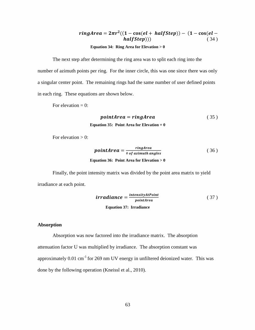
63

𝒓𝒊𝒏𝒈𝑨𝒓𝒆𝒂 = 𝟐𝝅𝒓𝟐((𝟏 − 𝐜𝐨𝐬(𝒆𝒍 + 𝒉𝒂𝒍𝒇𝑺𝒕𝒆𝒑)) − (𝟏 − 𝐜𝐨𝐬(𝒆𝒍 − 𝒉𝒂𝒍𝒇𝑺𝒕𝒆𝒑))) ( 34 )

Equation 34: Ring Area for Elevation > 0

The next step after determining the ring area was to split each ring into the

number of azimuth points per ring. For the inner circle, this was one since there was only

a singular center point. The remaining rings had the same number of user defined points

in each ring. These equations are shown below.

For elevation = 0:

𝒑𝒐𝒊𝒏𝒕𝑨𝒓𝒆𝒂 = 𝒓𝒊𝒏𝒈𝑨𝒓𝒆𝒂 ( 35 ) Equation 35: Point Area for Elevation = 0

For elevation > 0:

𝒑𝒐𝒊𝒏𝒕𝑨𝒓𝒆𝒂 = 𝒓𝒊𝒏𝒈𝑨𝒓𝒆𝒂# 𝒐𝒇 𝒂𝒛𝒊𝒎𝒖𝒕𝒉 𝒂𝒏𝒈𝒍𝒆𝒔

( 36 )

Equation 36: Point Area for Elevation > 0

Finally, the point intensity matrix was divided by the point area matrix to yield

irradiance at each point.

𝒊𝒓𝒓𝒂𝒅𝒊𝒂𝒏𝒄𝒆 = 𝒊𝒏𝒕𝒆𝒏𝒔𝒊𝒕𝒚𝑨𝒕𝑷𝒐𝒊𝒏𝒕𝒑𝒐𝒊𝒏𝒕𝑨𝒓𝒆𝒂

( 37 )

Equation 37: Irradiance

Absorption

Absorption was now factored into the irradiance matrix. The absorption

attenuation factor U was multiplied by irradiance. The absorption constant was

approximately 0.01 cm-1 for 269 nm UV energy in unfiltered deionized water. This was

done by the following operation (Kneissl et al., 2010).

64

𝒂𝒃𝒔𝒐𝒓𝒑𝒕𝒊𝒐𝒏 = 𝒊𝒓𝒓𝒂𝒅𝒊𝒂𝒏𝒄𝒆 ∗ 𝒆−𝒂∗𝒓 ( 38 ) Equation 38: Absorption

Table 18 shows absorption coefficients for four types of water used in an

experiment to test UV LED disinfection rates. These constants show that tap water,

surface water, and secondary effluent absorb much more energy than deionized water.

Figure 25 shows the effect of altering the absorption coefficient. The absorption constant

was first set to 0 to show the effect of no absorption. Then the absorption rate was

stepped through the absorption values for deionized water, tap water, surface water, and

secondary effluent. It is clear that absorption greatly reduces the effect of an LED bulb

(Kneissl et al., 2010).

The table also showed that filtered water has a lower absorption coefficient than

unfiltered water. Suspended solids in unfiltered water cause this effect. In addition to

increasing the absorption coefficient, suspended solids may also build up residue within

the vessel. This may decrease reflection from the vessel walls and energy output from

the bulbs (Lenk & Lenk, 2011; Wurtele et al., 2011).

Table 18: Absorption Coefficients for Common Types of Water (Kneissl et al., 2010)

Parameter Unit

Deionised Water (DI)

Tap Water (TW)

Surface Water (SW)

Secondary Effluent (SE)

unfil

tere

d

A (254) [1/m] 1.1 8.8 19 29.2

A (269) [1/m] n.a. 7.7 17.1 26.6

filte

red

A (254) [1/m] 0.8 8.5 17.6 28.2

A (269) [1/m] n.a. 7.5 15.7 25.7

65

Figure 25: Single Bulb, 300 μW, Top a=0 cm-1, Middle Left a=0.01 cm-1, Middle Right a=0.077 cm-1,

Bottom Left a=0.171 cm-1, Bottom Right a=0.266 cm-1

Spherical to Cartesian Conversion

Three operations were performed to convert the spherical coordinates used up to

this point into a Cartesian system that was able to be used in MATLAB to plot in three

66

dimensions. The first process was a simple conversion of spherical to Cartesian

coordinates. After this was completed, the Cartesian coordinates were moved to the

closest 0.1 cm interval. Finally the matrices were reordered to allow the x, y, and z

coordinates to be arranged in increasing value.

MATLAB’s ‘sph2cart’ command was used to convert the spherical coordinates to

Cartesian coordinates. Azimuth and elevation were first converted to radians, as required

by MATLAB. The output of this command was x, y, and z matrices that was ordered

according to the initial spherical system.

The function ‘conversion’ was used to move the x, y, and z coordinates to the

closest 0.1 cm grid. This function stepped through each data point in the x, y, and z

coordinate matrices and moves the coordinate to the closest grid location. This

movement introduced error into the model. A smaller grid size reduced the error, but

resulted in a longer computing time if adequate computing memory was even available.

Finally, the function ‘reOrder’ was used to rearrange the Cartesian coordinate and

irradiance matrices to order the coordinates in increasing value. Each data point was

called and stepped through a 0.1 cm grid. The irradiance at a point was added to the re-

ordered matrix when the x, y, and z coordinates matched the correct grid location. At this

point the irradiance matrix was set up for MATLAB’s three dimensional graphing

functions.

Bulb Array

The function ‘bulbOffset’ was used to add multiple bulbs. The metric units for

the LEDs in Table 5, above, were used for the LED placement. The function rounded the

67

units to the closest 0.1 cm interval to use the same spacing requirement as used in the

coordinate conversion steps. The function added one LED at a time with the x and y

displacement. The intensity for each point in the multiple LED array was summed into a

matrix named ‘multipleBulbs’.

Limit Bulb Array

The function ‘cut’ was used to limit the irradiance matrix to inside the vessel and

for the fluid height in the vessel. The function called each point in the matrix passed into

the function. The value of irradiance at any point was set to zero if the radius of the point

from the center of the vessel was greater than the radius of the vessel, or the height of the

point exceeded the fluid height of the system. The fluid height variable must be set equal

to the vessel height for flow through systems.

Pathogen Inactivation

DNA Disruption – Batch

The dose-log inactivation equation for Bacillus subtilis spores was obtained from

experiments conducted by Wurtele et. al and is shown in Equation 39. This equation was

obtained from data taken from 117 to 233 J/m2. ‘Dose’ was measured in J/m2 (Wurtele et

al., 2011).

𝑳𝒐𝒈 𝑰𝒏𝒂𝒄𝒕𝒊𝒗𝒂𝒕𝒊𝒐𝒏 = 𝟎.𝟎𝟏𝟑𝟑 𝒅𝒐𝒔𝒆 + 𝟎.𝟓𝟓𝟒𝟕 ( 39 ) Equation 39: Dose-Log Inactivation for 269 nm LED Bulbs

This equation did not account for the shoulder and tailing regions. Instead it only

represented the log-linear region. The MATLAB code was adjusted for this by limiting

dose to only be valid at or above 117 J/m2. This threshold was chosen since that was the

68

smallest data point recorded in the experiment. If a lower limit was not selected, then a

dose of 0 J/m2 would calculate to a log reduction of 0.5547 when there should be no log

reduction.

Mix time was defined as the time required for the solution to completely mix and

re-initialize as a singular concentration due to the stirrer in the vessel. The calculations

behind the log reduction assumed that the fluid was relatively stable during the mix time

and averaged with the rest of the solution after each mix period. One final mix period

was performed for the remainder when experiment times were not evenly divisible by the

mix time.

Tran’s (2014) experiments consisted of measuring the log reduction of bacillus

globigii spores in a batch environment. The reactor vessel was placed on an orbital

shaker to mix the solution in the reactor without introducing a mixing device within the

vessel. The reactor was oriented with the bulb plate on the bottom and the bulbs facing

up. A solution of deionized water and spores with an initial concentration of 7x106 was

used to fill the vessel with 100 ml. This resulted in a calculated fluid height of 2.396 cm

in the vessel. Figure 26 shows the set up for Tran’s experiments. Tran ran multiple trials

with durations of 64 and 129 seconds. Table 19 shows the log reduction associated with

both duration times.

69

Figure 26: Tran's Set Up (Tran, 2014)

Table 19: Batch Experiment Results

Duration Log Kill 64 s .5-.6

129 s 1.5

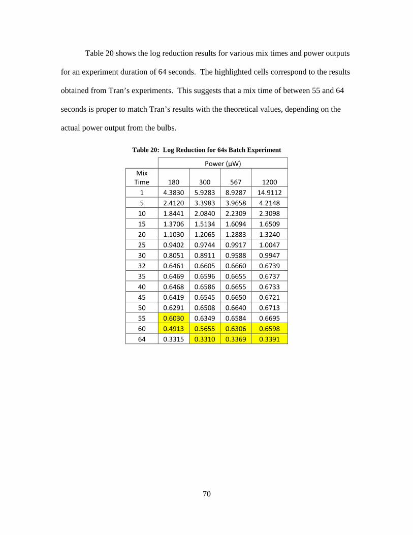
70

Table 20 shows the log reduction results for various mix times and power outputs

for an experiment duration of 64 seconds. The highlighted cells correspond to the results

obtained from Tran’s experiments. This suggests that a mix time of between 55 and 64

seconds is proper to match Tran’s results with the theoretical values, depending on the

actual power output from the bulbs.

Table 20: Log Reduction for 64s Batch Experiment

Power (µW)

Mix Time 180 300 567 1200

1 4.3830 5.9283 8.9287 14.9112 5 2.4120 3.3983 3.9658 4.2148

10 1.8441 2.0840 2.2309 2.3098 15 1.3706 1.5134 1.6094 1.6509 20 1.1030 1.2065 1.2883 1.3240 25 0.9402 0.9744 0.9917 1.0047 30 0.8051 0.8911 0.9588 0.9947 32 0.6461 0.6605 0.6660 0.6739 35 0.6469 0.6596 0.6655 0.6737 40 0.6468 0.6586 0.6655 0.6733 45 0.6419 0.6545 0.6650 0.6721 50 0.6291 0.6508 0.6640 0.6713 55 0.6030 0.6349 0.6584 0.6695 60 0.4913 0.5655 0.6306 0.6598 64 0.3315 0.3310 0.3369 0.3391

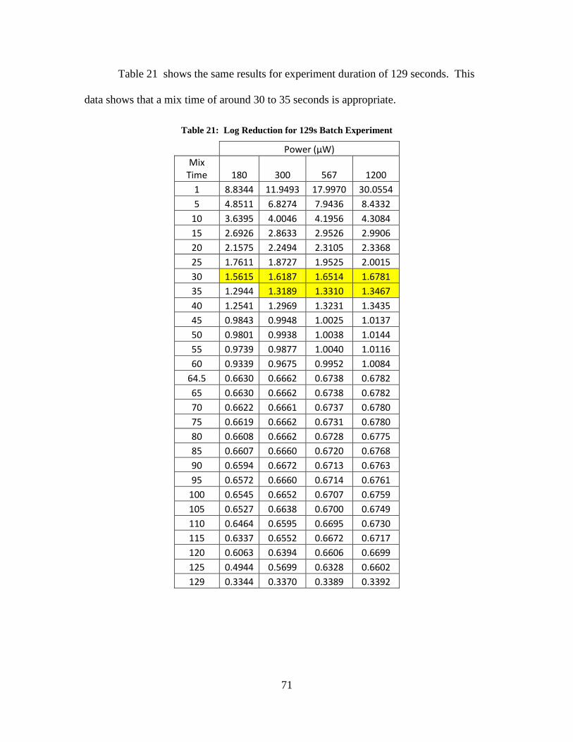
71

Table 21 shows the same results for experiment duration of 129 seconds. This

data shows that a mix time of around 30 to 35 seconds is appropriate.

Table 21: Log Reduction for 129s Batch Experiment

Power (µW)

Mix Time 180 300 567 1200

1 8.8344 11.9493 17.9970 30.0554 5 4.8511 6.8274 7.9436 8.4332

10 3.6395 4.0046 4.1956 4.3084 15 2.6926 2.8633 2.9526 2.9906 20 2.1575 2.2494 2.3105 2.3368 25 1.7611 1.8727 1.9525 2.0015 30 1.5615 1.6187 1.6514 1.6781 35 1.2944 1.3189 1.3310 1.3467 40 1.2541 1.2969 1.3231 1.3435 45 0.9843 0.9948 1.0025 1.0137 50 0.9801 0.9938 1.0038 1.0144 55 0.9739 0.9877 1.0040 1.0116 60 0.9339 0.9675 0.9952 1.0084

64.5 0.6630 0.6662 0.6738 0.6782 65 0.6630 0.6662 0.6738 0.6782 70 0.6622 0.6661 0.6737 0.6780 75 0.6619 0.6662 0.6731 0.6780 80 0.6608 0.6662 0.6728 0.6775 85 0.6607 0.6660 0.6720 0.6768 90 0.6594 0.6672 0.6713 0.6763 95 0.6572 0.6660 0.6714 0.6761

100 0.6545 0.6652 0.6707 0.6759 105 0.6527 0.6638 0.6700 0.6749 110 0.6464 0.6595 0.6695 0.6730 115 0.6337 0.6552 0.6672 0.6717 120 0.6063 0.6394 0.6606 0.6699 125 0.4944 0.5699 0.6328 0.6602 129 0.3344 0.3370 0.3389 0.3392

72

Since the mix times are a rough generalization of fluid flow in the batch reactor,

the mixing rate for the 64 second and 129 second experiments do not match. A program

or process that adequately calculates fluid flow in a batch reactor is needed.

AOP - Flow

Radical production may follow a linear relationship with input variables of UV

energy and oxidant concentration. The rate of change is dependent on the specific

applied energy and the oxidant type. Little research is available in this area, which

mainly describes a rate constant based off of a starting concentration and an overall dose.

Literature does not state if AOPs follow a linear dose to log-reduction curve or if regions

are present as in DNA disruption. This research calculated the total dose applied within

the reaction vessel for the flow through experiments.

The flow through experiments were set up with the solution entering the vessel

through the inlet pipe on the bottom of the vessel. Then the solution traveled through the

vessel and exited by the discharge pipe located on the top of the vessel. The LED plate

faced horizontally along the reactor on the side closer to the discharge pipe. Duckworth’s

(2014) set up is shown in Figure 27.

73

Figure 27: Duckworth's Set Up (Duckworth, 2014)

A basic dose calculation for flow was conducted to determine the dose that was

exposed to the solution flowing through the reaction vessel. This calculation represented

the applied dose for flow that began at the inlet. This does not apply to the initial fluid in

the vessel that started part way through the vessel, since when this process is applied in

real world applications, the reactor may be primed with a neutralized solution. The flow

was also assumed to be laminar and constant through the vessel. The calculation used a

flow rate of 1.4 mL/min to match the experiments conducted by Duckworth (2014). The

total dose for each power output is reported in Table 22. The applied dose was between

6.42x109 and 4.28x1010 mJ/cm2. A more specific dose was not determined because the

LEDs were not measured directly before or after testing.

74

Table 22: Flow Dose with Varying Bulb Output Power

Dose (mJ/cm2)

180 μW 6.42E+09 300 μW 1.07E+10 567 μW 2.02E+10 1200 μW 4.28E+10

Graphing

MATLAB’s graphing function ‘contourslice’ was used to visualize the three

dimensional irradiance patterns. Graphs were called to show irradiance values of less

than 1 mW/cm2, 1-200 mW/cm2, and greater than 200 mW/cm2. These ranges were used

to show the shoulder, linear, and tailing regions set forth by the EPA for DNA disruption.

These ranges are useful in either batch or flow experiments for this reactor vessel.

75

Figures 28 and 29 show a singular bulb and the bulb array with extents limited to

the vessel dimensions at the three regions. Each region was nested inside each other.

The log-linear region overlapped with adjacent bulbs in the bulb array configuration.

Figure 28: Bulb at 300 μW with Nested Shoulder, Linear, and Tailing Regions

Figure 29: Bulb Array at 300 μW with Nested Shoulder, Linear, and Tailing Regions

Figures 30 to 32 show the shoulder, linear and tailing regions for a single SETi

UVTOP260 TO-39 FW bulb. Each figure shows the bulb with the minimum and typical

power specifications stated on the manufacturer’s specification sheet on the top row

followed by the average value measured by the manufacturer prior to shipment and the

average value measured locally.

Figure 30 shows irradiance from 0.1 to 1 mW/cm2 for a single LED limited to the

height and radius of the vessel. This was in the shoulder region where DNA repair

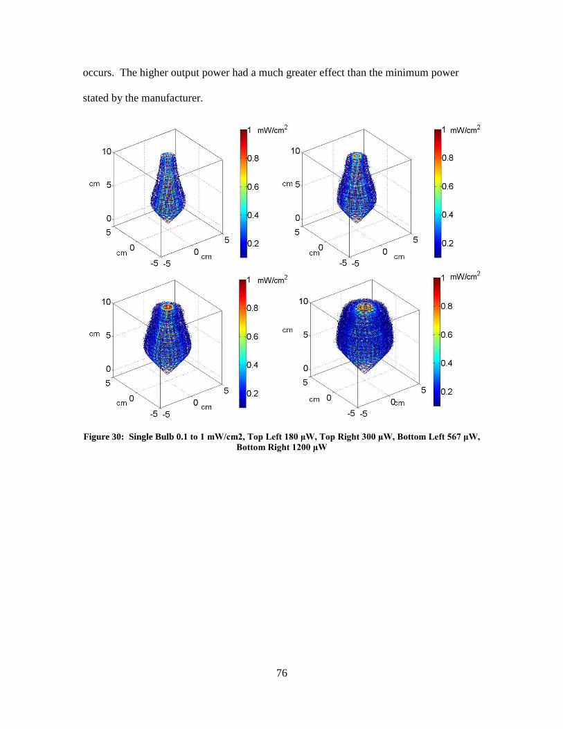
76

occurs. The higher output power had a much greater effect than the minimum power

stated by the manufacturer.

Figure 30: Single Bulb 0.1 to 1 mW/cm2, Top Left 180 μW, Top Right 300 μW, Bottom Left 567 μW,

Bottom Right 1200 μW

77

Figure 31 shows the linear region, which was nested inside the shoulder region.

This volume was where DNA repair did not occur and was inside the tailing region. The

volume greatly changed for the different output power of the bulbs.

Figure 31: Single Bulb 1 to 200 mW/cm2, Top Left 180 μW, Top Right 300 μW, Bottom Left 567

μW, Bottom Right 1200 μW

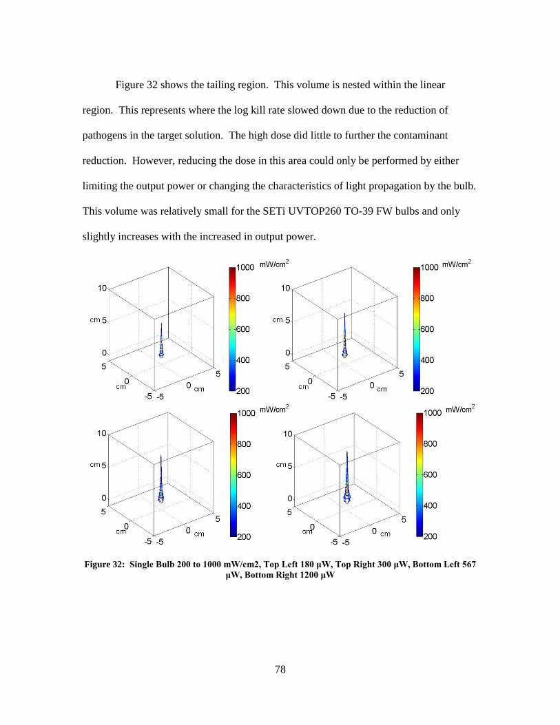
78

Figure 32 shows the tailing region. This volume is nested within the linear

region. This represents where the log kill rate slowed down due to the reduction of

pathogens in the target solution. The high dose did little to further the contaminant

reduction. However, reducing the dose in this area could only be performed by either

limiting the output power or changing the characteristics of light propagation by the bulb.

This volume was relatively small for the SETi UVTOP260 TO-39 FW bulbs and only

slightly increases with the increased in output power.

Figure 32: Single Bulb 200 to 1000 mW/cm2, Top Left 180 μW, Top Right 300 μW, Bottom Left 567


79

Figures 33 through 35 show the same regions for the bulb array. Figure 33 shows

that almost all of the volume was covered by the minimum output power guaranteed by

the manufacturer for the shoulder region. The only area outside this region was outside

the emission angle of each bulb located at the bottom of the vessel.

Figure 33: Bulb Array 0.1 to 1 mW/cm2, Top Left 180 μW, Top Right 300 μW, Bottom Left 567 μW,

Bottom Right 1200 μW

80

Figure 34 shows the volume covered by the linear region in the multiple bulb

configuration. The area increased as the power increased. The area between the energy

propagation was almost nonexistent for the 567 μW power output and did not exist for

the 1200 μW power output.

Figure 34: Bulb Array 1 to 200 mW/cm2, Top Left 180 μW, Top Right 300 μW, Bottom Left 567


81

The tailing region, shown in Figure 35, did not overlap between the energy

propagated from the separate bulbs. This illustrates that the maximum log reduction in

the vessel was not limited by overpowering due to the bulb array configuration, but from

the individual bulbs themselves.

Figure 35: Bulb Array 200 to 1000 mW/cm2, Top Left 180 μW, Top Right 300 μW, Bottom Left 567


Reactor Vessel Optimization

The measures for DNA disruption and AOP are different. Reactor vessels for

DNA disruption are optimized when they reach the greatest efficiency to neutralize target

pathogens. DNA disruption followed a log reduction curve that had a shoulder, log-

linear, and tailing regions. AOPs may lack the shoulder, log-linear, and tailing curve

82

where some regions are less effective than others. Batch and flow vessels may also alter

the optimum design of the reactor.

DNA Disruption Conclusions

Reactor vessels are optimized for DNA disruption applications when the percent

by volume for the log-linear region is the greatest. This ensures that the optimal dose

range is present in the greatest volume of the vessel. Table 23 shows the percent by

volume for the three regions for varying power output for the bulb array. The log-linear

region greatly increased with the given power outputs while the tailing region slightly

increased. Throughout this process, the shoulder region significantly decreased.

Table 23: Percent Volume Associated with Shoulder, Log-Linear, and Tailing Regions

180 μW

300 μW

Count Percent

Count Percent

Shoulder 153432 55.49%

Shoulder 105000 37.97% Log-Linear 120562 43.60%

Log-Linear 167901 60.72%

Tailing 2534 0.92%

Tailing 3619 1.31%

567 μW

1200 μW

Count Percent

Count Percent

Shoulder 41384 14.97%


Log-Linear 262968 95.10%

Tailing 5646 2.04%

Tailing 9268 3.35%

Table 24 shows results for the same bulb spacing and vessel size with a power

output of 3000 μW. This illustrates that the vessel radius is smaller than the optimized

radius for the same fluid height due to the decrease in the log-linear region when

compared to bulbs with 1200 μW output power. The higher output bulbs provide a

higher dose, but the energy output to disinfection rate is reduced.

83

Table 24: Percent Volume Associated with Shoulder, Log-Linear, and Tailing Regions for 3000 μW

3000 μW

Count Percent


Tailing 18814 6.80%

The bulb array was dependent on the power output of the bulbs and the ranges of

the shoulder, log-linear, and tailing regions. The goal was to reduce the volume

containing the shoulder region, while increasing the volume containing the log-linear

region. The tailing region was where overpowering occurs, but this was a direct result

from the bulb specifications. This goal results in a higher disinfection to energy output

rate. The tailing region may be reduced by obtaining LEDs with a different energy

spread. Otherwise, this region was accepted as a necessary less efficient volume than the

log-linear region volume. However, the minimum this region should be in a reactor

vessel was the size of this region for a single bulb, multiplied by the number of bulbs in

the reactor. Co-locating bulbs on opposite plates to overlap the tailing region may

provide data that shows a decrease in the tailing region, but this only further overpowers

the tailing volume. A better approach is to not overlap the tailing regions for a single

bulb. Design needs to ensure that the overlap of the energy spread does not produce

excess volume in the tailing region.

Utilizing the same vessel shape, another LED plate may be used on the opposite

side of the reactor to eliminate the void space near the bottom plate that receives no

energy and increase the areas in the shoulder region. The two bulb plates may be

designed to offset the bulbs so the tailing regions are not co-located. The energy pattern

84

also must be analyzed to reduce any excess tailing region volume. An ideal situation

would involve LED bulbs that do not emit in the tailing region, which also creates an

energy pattern fully in the log-linear region.

AOP Conclusions

The limited available literature on AOPs suggests that radical production is

dependent on UV dose and initial oxidant concentration. Therefore, the optimal vessel

design would involve applying the optimal UV and oxidant doses to reach a given

contaminant reduction for every fluid path in the vessel.

Batch Reactor Conclusions

Batch and flow applications affect reactor design. These applications greatly

differ in how dose is applied and in fluid movement within the reactor. Batch reactors

may be best suited for small scale home or individual water disinfection systems, while

flow through reactors may be best suited for large scale commercial applications.

Batch reactor design must account for sediment and achieve an even dose

throughout the vessel. Sediment in the reactor may block energy propagation.

Depending on the sediment density, it may fall, suspend, or float in the reactor. Bulb

placement may be decided based on the anticipated sediment in the reactor. For example,

place the LEDs on the top of the vessel if the sediment tends to fall. In this case, the fluid

may be placed in the reactor for a given time prior to disinfection to allow the sediment to

collect prior to energizing the system. Another option is to filter the fluid to remove

particles, which may also filter microbes. The batch experiments conducted by Tran

(2014) shook the system since the LED array was placed on the bottom plate. This

prevented the spores from collecting on the bottom plate which could increase the

85

absorption coefficient closer to the bulbs and increase the concentration of spores located

in the system outside the emission angle of any of the bulbs. The orbital shaking also

mixed the solution to spread the applied dose more evenly throughout the fluid. An even

dose may be applied by arranging the LED array to provide an even intensity throughout

the vessel. The gaps between the bulbs on a single plane may be eliminated by placing

bulbs on multiple planes.

Fluid Flow Reactor Conclusions

Flow through reactor designs must account for fluid flow. The fluid path must be

analyzed to correctly apply an energy distribution in the system to guarantee a minimum

dose applied to every path through the reactor. A conservative method may involve

determining the quickest path through the vessel and applying a minimum intensity

throughout the vessel to achieve the required dose along this quickest path. Sediment

collecting in the reactor may be an issue depending on flow velocity. Two methods to

circumvent this are to increase the flow rate to not allow sediment collection and filter the

fluid prior to entering the reactor, which may also filter the organisms.

Designing a system for laminar flow eases the process to build the correct bulb

array. However, large flow requirements may prevent a laminar system from being

possible. Pipe friction reduces the flow velocity around the reactor walls. This drives an

uneven required spread of energy in the system since the contact time near the reactor

walls is higher than the quicker velocity towards the center of the reactor.

86

Concepts for Future Flow Reactor Designs

Fluid Flow

The basics of fluid flow in a closed vessel involve laminar versus turbulent flow

and flow velocity through the vessel. Laminar flow may be beneficial in flow through

reactors due to more predictable flow paths. Whether the flow is laminar or turbulent

depends on a few factors. The vessel shape and fluid velocity play a major role in this.

Areas where the vessel changes shape may change laminar flow to turbulent flow. Flow

velocity alone may also determine if a flow is laminar or turbulent through a constant

geometry.

Internal wall friction prevents constant fluid flow. The flow is slower closer to

the reactor walls and is the quickest in the middle of a flow through reactor. Smoother

vessel walls reduce the velocity differences and provide a better surface for reflection.

Pipe Designs

Mercury lamp flow through reactors are traditionally based off of a pipe with

mercury lamps in a quartz tube placed parallel or perpendicular to the flow, as discussed

in Chapter II. LEDs are able to eliminate the need for the quartz tube interface in reactor

vessels. The traditional pipe design may be used with LEDs around the exterior of the

reactor. Figure 36 shows an example of this design with four evenly spaced bulbs around

the outside of the pipe and the resulting fields of view with the SETi bulbs in water. The

cross sectional four-bulb array may repeat along the length of the pipe and be rotated to

level the irradiance field along the pipe.

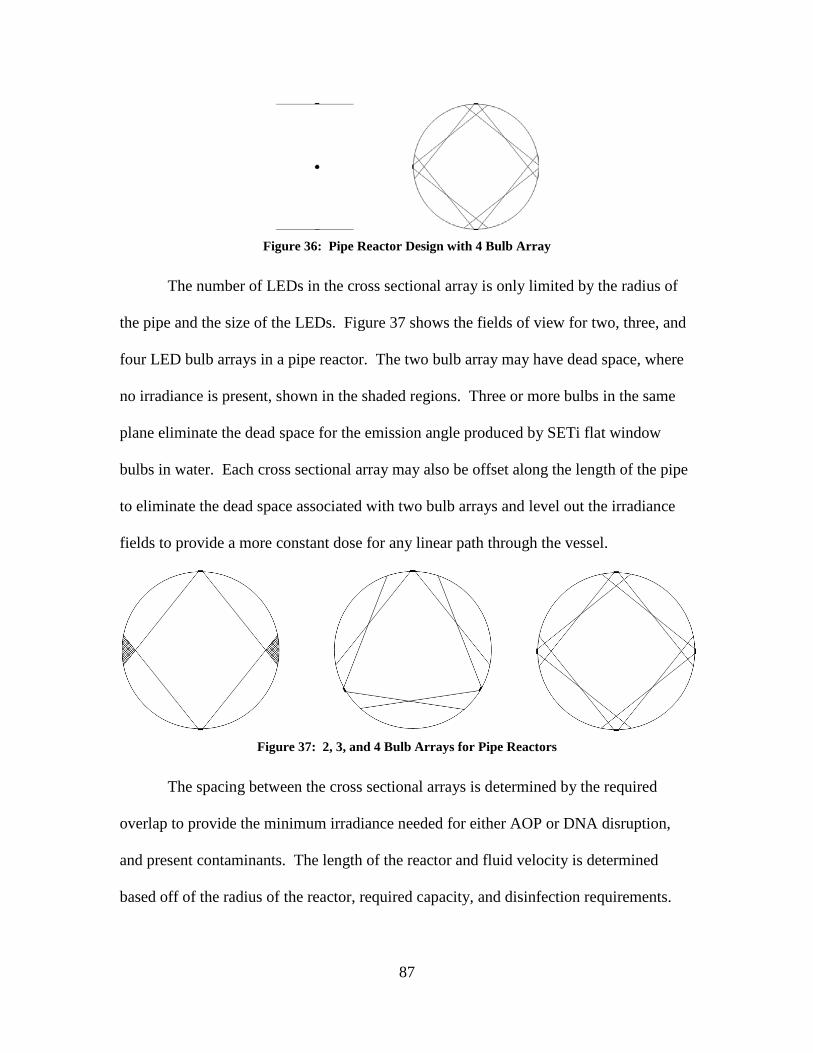
87

Figure 36: Pipe Reactor Design with 4 Bulb Array

The number of LEDs in the cross sectional array is only limited by the radius of

the pipe and the size of the LEDs. Figure 37 shows the fields of view for two, three, and

four LED bulb arrays in a pipe reactor. The two bulb array may have dead space, where

no irradiance is present, shown in the shaded regions. Three or more bulbs in the same

plane eliminate the dead space for the emission angle produced by SETi flat window

bulbs in water. Each cross sectional array may also be offset along the length of the pipe

to eliminate the dead space associated with two bulb arrays and level out the irradiance

fields to provide a more constant dose for any linear path through the vessel.

Figure 37: 2, 3, and 4 Bulb Arrays for Pipe Reactors

The spacing between the cross sectional arrays is determined by the required

overlap to provide the minimum irradiance needed for either AOP or DNA disruption,

and present contaminants. The length of the reactor and fluid velocity is determined

based off of the radius of the reactor, required capacity, and disinfection requirements.

88

Manufacturing is one major drawback of pipe reactors with flat window LED

bulbs. Placing a flat window on a curved surface requires high part tolerances.

Rectangular designs ease LED installation.

Rectangular Designs

Utilizing bulb arrays on two reactor walls in rectangular designs eliminates dead

space in the reactor. The arrays may be offset to eliminate peaks from the upper and

lower arrays from overlapping. Figure 38 shows a general rectangular reactor design.

The black circles represent LEDs on the upper reactor wall and red circles represent

LEDs on the lower reactor wall.

Figure 38: Rectangular Reactor Design

The LED bulb layout and spacing needs to be optimized based off of bulb

characteristics, disinfection method, and inactivation requirements. The reactor height,

reactor width and array length also need to be optimized to provide the required capacity.

Normally, fluid is conveyed through circular pipes. A rectangular reactor may require a

volume before and after the bulb array to allow the fluid to transition from a circular to

rectangular geometry and provide a laminar flow through the volume exposed to UV

energy.

89

Modular Design

In either pipe or rectangular designs, reactors may be split into modules to

increase the uses for a single reactor. The modules may be designed in series or parallel.

The series designs allow separate bulb arrays to operate as needed. Parallel designs may

open reactor chambers as needed. The bulb arrays may be placed sequentially or overlap

to provide the needed flexibility throughout the system’s life.

Modular designs allow a single system to increase dose based when required.

These designs also enable systems to increase or decrease inactivation capacity based off

of need. This flexibility also changes energy usage to either slow or speed up the system

to prevent shutting the system down, while not wasting energy by overpowering slow

fluid velocities.

Chapter Summary

In this chapter, the data and results from the modeling and simulation are

presented. This work is compared to results collected from laboratory experiments and

differences are noted. The next chapter presents conclusions from this research and

concepts for future reactor designs with LED bulbs.

90

V. Conclusions

Chapter Overview

This chapter explains the main conclusions of this research stream, followed by

why it is important. Next, research limitations are stated. Finally, recommendations for

future research are presented.

Conclusions of Research

This research presented a methodology to model UV LEDs in reactor vessels.

Energy propagation patterns were used to determine irradiance in a reaction vessel for

both batch and flow experiments. The irradiance patterns were used to illustrate how to

optimize vessels to achieve log reduction requirements by both DNA disruption and AOP

methods. The initial research questions are answered below.

RQ1: What is an Advanced Oxidation Process (AOP) and DNA disruption?

How are they different and similar? Also, how are they used for water

disinfection?

Chapter II discusses AOP and DNA disruption in more detail. The AOP involves

adding a chemical that breaks down into radicals when the optimal wavelength of energy

is applied. These radicals subsequently react with the contaminants to transform them.

In Duckworth’s (2014) research, hydrogen peroxide (H2O2) was converted by UV energy

into hydroxyl radicals (∙OH), which reacted with methylene blue, an indicator dye. DNA

disruption affects the chemical structure of the targeted pathogens. This neutralizes the

pathogen and prevents reproduction from occurring.

91

RQ2: What sources of ultraviolet (UV) radiation have been used for the AOP

and DNA disruption in water disinfection applications?

This question is also addressed in Chapter II. Mercury lamps are the predominant

UV energy source due to their high power output and market availability. UV LEDs are

an emerging technology for water disinfection. They are relatively new, have low power

output, and have short lifespans. Many experts agree that UV LEDs will follow the

advancements of visible light LEDs and improve in the coming years.

RQ3: What are the measures of UV energy distribution in a reactor vessel?

Chapter II discusses the measures of UV energy distribution. The measures are

different for DNA disruption and AOPs. DNA disruption follows a shoulder, log-linear,

and tailing regions. The log-linear region has the most efficient disinfection rate of the

three regions. Literature suggests that radical formation has a linear relationship with UV

energy in an AOP. More research is needed to show the relationship between radical

concentration and organic oxidation.

RQ4: What mathematical models can be used to calculate the distribution and

absorption of UV Light Emitting Diode (LED) radiation as it propagates

through different mediums?

Chapter III describes the equations and models used to determine energy

propagation. LED energy propagation is vastly different than the predominant mercury

lamp technology in water disinfection. The basic mercury lamp models assume

92

Lambertian attributes, which do not describe LED energy propagation. Modeling LED

energy propagation involves un-normalizing the manufacturer’s specifications for energy

distribution and calculating the energy and area associated with each point in the reactor.

Absorption is applied based on the distance away from the energy source. Different

mediums change the absorption coefficient and the emission angle of the LEDs.

RQ5: What tools can be used to simulate these models to calculate the UV

energy present at any point within a UV reactor vessel?

Chapters II and III discuss the tools that can be used to model UV energy.

MATLAB is excellent to manipulate data arrays to calculate energy distribution, but

lacks fluid flow capability. COMSOL Multiphysics offers fluid modules to account for

fluid flow through a reactor. This platform may be best to optimize LED bulb

arrangement for fluid flow through a reactor.

RQ6: How do simulation results generated from the model compare to actual

experimental results collected from the laboratory?

Chapter IV discusses the results obtained from the laboratory and the model. The

batch experiments utilize DNA disruption which has better dose-log reduction equations

in literature. A mix time was applied to the model to generalize the effect of mixing in

the vessel. However, the mix time for the 64 and 129 second duration experiments did

not match. The limited equation from literature for these experiments also restricts the

accuracy of the model. The flow through experiments utilize AOP to generate hydroxyl

93

radicals. Further research needs to be conducted to fill the knowledge gap of dose to

hydroxyl radical production to properly model the results.

RQ7: What UV LED reactor designs are most efficient for water disinfection?

Chapter IV discusses optimized reactor designs. The application drives design

choices for batch or flow, while disinfection method determines vessel geometry. The

required flow determines if batch or flow is appropriate. Smaller scale systems may be

best in batch applications since the reactor is less complex. On the other hand flow

systems may be used to treat larger quantities of fluid. DNA disruption or AOP

determines the optimal LED arrangement. DNA disruption seeks to optimize the log-

linear region and optimal dose while AOP only seeks to optimize a constant dose to all of

the fluid.

Significance of Research

This research addressed the difference in modeling UV LED bulbs compared to

mercury lamps. Mercury lamps propagate energy following Lambertian behavior. This

is not the case with LEDs. They have a limited emission angle that reduces in power

towards the extent of this angle.

The presented methodology illustrated how to model energy propagation for

LEDs to determine reactor vessel shape and size. This research is useful to create reactor

vessels that replace mercury lamps with UV LEDs. The approach may also be used in

other UV LED applications, such as curing in a manufacturing setting.

94

Limitations

The main limitations of this research are limited knowledge of energy outputs

throughout the experiments conducted in the laboratory, log reduction rates compared to

applied dose, and fluid flow. The actual output power was not known for the multiple

experiments due to exponential output power degradation in the first 100 hours of run

time. This research based the applied dose to log reduction rate of Bacillus subtilis

spores on data that only describes the log-linear region. Assumptions were made to

supplement the data for the shoulder and tailing regions. Finally, fluid flow through the

vessel was not addressed. Assumptions were made that constant, laminar flow occurred

throughout the vessel for flow applications and a generalization for mix rate in batch

applications.

Recommendations for Future Research

Follow on research is necessary to tune the model for specific water disinfection

applications and optimize reactor vessels. These research streams are described below.

Tune Model

1) Collimated Beam Experiments: The model can be applied with these

experiments to determine the log reduction function, dependent on dose, for

various contaminants. The trials need to determine the shoulder, log-linear,

and tailing regions along with the associated log reduction.

2) Fluid Flow: The model can be refined by accounting for fluid flow in reactor

vessels. The fluid modules in COMSOL Multiphysics may be the correct

tool.

95

Optimize Reactor Vessels

1) Compare UV LED Bulbs: A comparison of LED windows and power output

can be performed to decrease the shoulder and tailing regions and optimize the

log-linear region.

2) Optimize Reactor Vessel Shape: A comparison of reactor vessel shapes can be

performed to determine optimized shapes for both batch and flow applications

for single bulbs and various bulb arrays.

3) Optimize Reactor Vessel Size for Various Uses: A comparison of reactor

vessel size can be optimized for various types of uses and quantities of

contaminated fluid.

4) Pulsing: Pulsing has shown increased energy efficiency in UV disinfection

systems. This may be researched with the previous research streams.

Summary

In this chapter, the conclusions of research are addressed along with the

significance of the findings. Limitations to this research are addressed followed by

recommendations for future research.

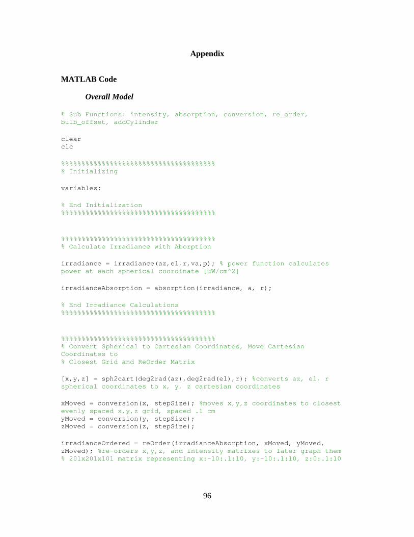
96

Appendix

MATLAB Code

Overall Model

% Sub Functions: intensity, absorption, conversion, re_order, bulb_offset, addCylinder clear clc %%%%%%%%%%%%%%%%%%%%%%%%%%%%%%%%%%%%%% % Initializing variables; % End Initialization %%%%%%%%%%%%%%%%%%%%%%%%%%%%%%%%%%%%%% %%%%%%%%%%%%%%%%%%%%%%%%%%%%%%%%%%%%%% % Calculate Irradiance with Aborption irradiance = irradiance(az,el,r,va,p); % power function calculates power at each spherical coordinate [uW/cm^2] irradianceAbsorption = absorption(irradiance, a, r); % End Irradiance Calculations %%%%%%%%%%%%%%%%%%%%%%%%%%%%%%%%%%%%%% %%%%%%%%%%%%%%%%%%%%%%%%%%%%%%%%%%%%%% % Convert Spherical to Cartesian Coordinates, Move Cartesian Coordinates to % Closest Grid and ReOrder Matrix [x,y,z] = sph2cart(deg2rad(az),deg2rad(el),r); %converts az, el, r spherical coordinates to x, y, z cartesian coordinates xMoved = conversion(x, stepSize); %moves x,y,z coordinates to closest evenly spaced x,y,z grid, spaced .1 cm yMoved = conversion(y, stepSize); zMoved = conversion(z, stepSize); irradianceOrdered = reOrder(irradianceAbsorption, xMoved, yMoved, zMoved); %re-orders x,y,z, and intensity matrixes to later graph them % 201x201x101 matrix representing x:-10:.1:10, y:-10:.1:10, z:0:.1:10

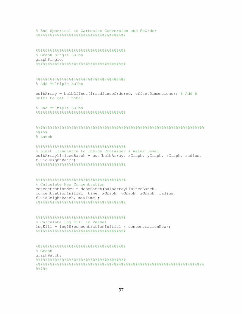
97

% End Spherical to Cartesian Conversion and ReOrder %%%%%%%%%%%%%%%%%%%%%%%%%%%%%%%%%%%%%% %%%%%%%%%%%%%%%%%%%%%%%%%%%%%%%%%%%%%% % Graph Single Bulbs graphSingle; %%%%%%%%%%%%%%%%%%%%%%%%%%%%%%%%%%%%%% %%%%%%%%%%%%%%%%%%%%%%%%%%%%%%%%%%%%%% % Add Multiple Bulbs bulbArray = bulbOffset(irradianceOrdered, offsetDimensions); % Add 6 bulbs to get 7 total % End Multiple Bulbs %%%%%%%%%%%%%%%%%%%%%%%%%%%%%%%%%%%%%% %%%%%%%%%%%%%%%%%%%%%%%%%%%%%%%%%%%%%%%%%%%%%%%%%%%%%%%%%%%%%%%%%%%%%%%%%%%% % Batch %%%%%%%%%%%%%%%%%%%%%%%%%%%%%%%%%%%%%% % Limit Irradiance to Inside Container & Water Level bulbArrayLimitedBatch = cut(bulbArray, xGraph, yGraph, zGraph, radius, fluidHeightBatch); %%%%%%%%%%%%%%%%%%%%%%%%%%%%%%%%%%%%%% %%%%%%%%%%%%%%%%%%%%%%%%%%%%%%%%%%%%%% % Calculate New Concentration concentrationNew = doseBatch(bulbArrayLimitedBatch, concentrationInitial, time, xGraph, yGraph, zGraph, radius, fluidHeightBatch, mixTime); %%%%%%%%%%%%%%%%%%%%%%%%%%%%%%%%%%%%%% %%%%%%%%%%%%%%%%%%%%%%%%%%%%%%%%%%%%%% % Calculate Log Kill in Vessel logKill = log10(concentrationInitial / concentrationNew); %%%%%%%%%%%%%%%%%%%%%%%%%%%%%%%%%%%%%% %%%%%%%%%%%%%%%%%%%%%%%%%%%%%%%%%%%%%% % Graph graphBatch; %%%%%%%%%%%%%%%%%%%%%%%%%%%%%%%%%%%%%% %%%%%%%%%%%%%%%%%%%%%%%%%%%%%%%%%%%%%%%%%%%%%%%%%%%%%%%%%%%%%%%%%%%%%%%%%%%%

98

%%%%%%%%%%%%%%%%%%%%%%%%%%%%%%%%%%%%%%%%%%%%%%%%%%%%%%%%%%%%%%%%%%%%%%%%%%%% % Dose %%%%%%%%%%%%%%%%%%%%%%%%%%%%%%%%%%%%%% % Limit Irradiance to Inside Container & Water Level bulbArrayLimitedFlow = cut(bulbArray, xGraph, yGraph, zGraph, radius, fluidHeightFlow); %%%%%%%%%%%%%%%%%%%%%%%%%%%%%%%%%%%%%% %%%%%%%%%%%%%%%%%%%%%%%%%%%%%%%%%%%%%% % Calculate Flow Dose Regions [doseTotal, doseShoulderTotal, doseLinearTotal, doseTailingTotal, countShoulder, countLinear, countTailing] = doseFlow(bulbArrayLimitedFlow, xGraph, yGraph, zGraph, radius, fluidHeightFlow, flowRate, shoulderMax, logLinearMax, stepSize); %%%%%%%%%%%%%%%%%%%%%%%%%%%%%%%%%%%%%% %%%%%%%%%%%%%%%%%%%%%%%%%%%%%%%%%%%%%% % Graph graphDose; %%%%%%%%%%%%%%%%%%%%%%%%%%%%%%%%%%%%%% %%%%%%%%%%%%%%%%%%%%%%%%%%%%%%%%%%%%%%%%%%%%%%%%%%%%%%%%%%%%%%%%%%%%%%%%%%%% Model = 'DONE'

Variables

%%%%%%%%%%%%%%%%%%%%%%%%%%%%%%%%%%%%%%%%%%%%%%%%%%%%%%%%% % User Input %%%%%%%%%%%%%%%%%%% % Vessel Parameters for Cylinder radius = 3.6449; %cm vesselHeight = 7.62; %cm %%%%%%%%%%%%%%%%%%% %%%%%%%%%%%%%%%%%%% % Bulb Array offsetDimensions = [-2.54,0;-1.27,2.20;-1.27,-2.20;0,0;1.27,2.20;1.27,-2.20;2.54,0]; %%%%%%%%%%%%%%%%%%% %%%%%%%%%%%%%%%%%%% % Bulb and Fluid Characteristics va = 39.72; %degrees p = 567; %180, 300, 567, 1200 uW a = .01; %1 per m for deionised water (DI) so .01 per cm to match units of r in cm %%%%%%%%%%%%%%%%%%%

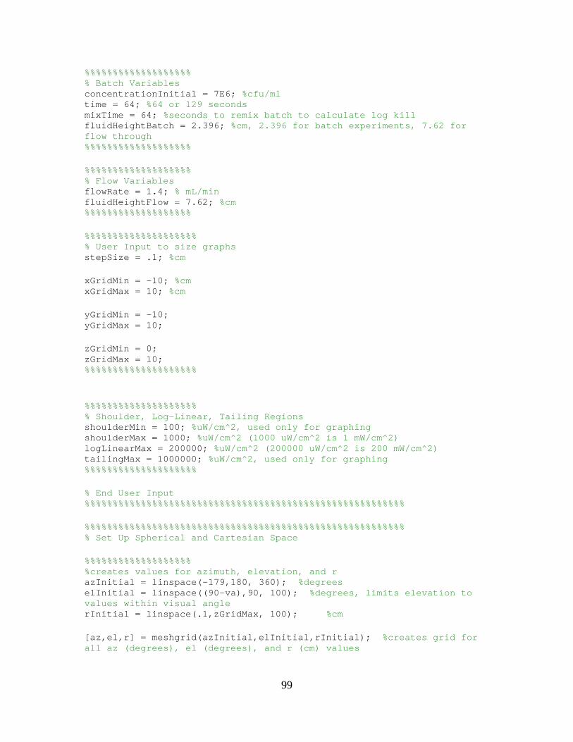
99

%%%%%%%%%%%%%%%%%%% % Batch Variables concentrationInitial = 7E6; %cfu/ml time = 64; %64 or 129 seconds mixTime = 64; %seconds to remix batch to calculate log kill fluidHeightBatch = 2.396; %cm, 2.396 for batch experiments, 7.62 for flow through %%%%%%%%%%%%%%%%%%% %%%%%%%%%%%%%%%%%%% % Flow Variables flowRate = 1.4; % mL/min fluidHeightFlow = 7.62; %cm %%%%%%%%%%%%%%%%%%% %%%%%%%%%%%%%%%%%%%% % User Input to size graphs stepSize = .1; %cm xGridMin = -10; %cm xGridMax = 10; %cm yGridMin = -10; yGridMax = 10; zGridMin = 0; zGridMax = 10; %%%%%%%%%%%%%%%%%%%% %%%%%%%%%%%%%%%%%%%% % Shoulder, Log-Linear, Tailing Regions shoulderMin = 100; %uW/cm^2, used only for graphing shoulderMax = 1000; %uW/cm^2 (1000 uW/cm^2 is 1 mW/cm^2) logLinearMax = 200000; %uW/cm^2 (200000 uW/cm^2 is 200 mW/cm^2) tailingMax = 1000000; %uW/cm^2, used only for graphing %%%%%%%%%%%%%%%%%%%% % End User Input %%%%%%%%%%%%%%%%%%%%%%%%%%%%%%%%%%%%%%%%%%%%%%%%%%%%%%%%% %%%%%%%%%%%%%%%%%%%%%%%%%%%%%%%%%%%%%%%%%%%%%%%%%%%%%%%%% % Set Up Spherical and Cartesian Space %%%%%%%%%%%%%%%%%%% %creates values for azimuth, elevation, and r azInitial = linspace(-179,180, 360); %degrees elInitial = linspace((90-va),90, 100); %degrees, limits elevation to values within visual angle rInitial = linspace(.1,zGridMax, 100); %cm [az,el,r] = meshgrid(azInitial,elInitial,rInitial); %creates grid for all az (degrees), el (degrees), and r (cm) values

100

%%%%%%%%%%%%%%%%%%%% %%%%%%%%%%%%%%%%%%%% % Size graphs xSteps = ((xGridMax - xGridMin)/stepSize)+1; %cm ySteps = ((yGridMax - yGridMin)/stepSize)+1; zSteps = ((zGridMax - zGridMin)/stepSize)+1; x1 = linspace(xGridMin,xGridMax,xSteps); %tenths y1 = linspace(yGridMin,yGridMax,ySteps); z1 = linspace(zGridMin,zGridMax,zSteps); [xGraph,yGraph,zGraph] = meshgrid(x1,y1,z1); % creates x,y,z matrixes to describe the points in the 'intensity' matrix %%%%%%%%%%%%%%%%%%%%% %%%%%%%%%%%%%%%%%%%%%%%%%%%%%%%%%%%%%%%%%%%%%%%%%%%%%%%%%

Irradiance

% calculates irradiance [uW/cm^2] based off of evenly spaced azimuth, elevation, and r function [ irradiance ] = irradiance(az,el,r,va,p) steradians = 2*pi*(1-cos(.5*(deg2rad(va)))); %calculates steradians based off of visual angle intensity = p/steradians; %calculates intensity based on power and angle shown through [uW/st] angle = 90-el; %calculates visual angle from center of light spread normalizedIntensityAtPoint = -2E-5*(angle.^3) + 6E-4*(angle.^2) - .0038*(angle) + .9702; %calculates normalized intensity value for each visual angle oSize = size(normalizedIntensityAtPoint); % Set center point azimuths to 0 except 1 value for i = 1:oSize(1); if el(i,1,1) == 90; %at 0 degrees from center (at center) normalizedIntensityAtPoint(i,2:oSize(2),1:oSize(3)) = 0; % set normalized intensity to zero except first azimuth angle so this doesn't add more than 1 point to center of beam end end

101

azSize = size(az); %number of data points in each ring normalizedTotalIntensityAtLayer = sum(sum(normalizedIntensityAtPoint)); %sums up intensity among all rings percentIntensityPoint = normalizedIntensityAtPoint(:,:,:) ./ normalizedTotalIntensityAtLayer(:,:,1); %percent intensity for each ring intensityAtPoint = percentIntensityPoint .* intensity; %calculates intensity at each point at distance r from bulb %%%%%%%%%%%%%%%%%%%%%%%%%%%%%%%%%%%%%%%%%%% % compute area associated with each point halfStep = (el(2,1,1) - el(1,1,1))/2; areaSize = size(intensityAtPoint); ringArea = zeros(areaSize(1), areaSize(2), areaSize(3)); pointArea = zeros(areaSize(1), areaSize(2), areaSize(3)); % Calculates Ring area for i = 1:areaSize(1); for j = 1:areaSize(2); for k = 1:areaSize(3); if 90 - el(i,j,k) == 0; ringArea(i,j,k) = 2*pi*r(i,j,k)^2 * (1-cos(deg2rad(halfStep))); %computes area associated with inner ring (circle) else ringArea(i,j,k) = (2*pi*r(i,j,k)^2 * (1-cos(deg2rad(90 - el(i,1,1) + halfStep)))) - (2*pi*r(i,j,k)^2 * (1-cos(deg2rad(90 - el(i,1,1) - halfStep)))); %computes area associated with all other rings end end end end % Calculates Point Area for i = 1:areaSize(1); for j = 1:areaSize(2); for k = 1:areaSize(3); if 90 - el(i,j,k) == 0;

102

pointArea(i,j,k) = ringArea(i,j,k); %leaves inner ring (circle) area at same value as ring (circle) area else pointArea(i,j,k) = ringArea(i,j,k) / azSize(2); %divides all other rings area by number of azimuth angle to obtain area per point end end end end %%%%%%%%%%%%%%%%%%%%%%%%%%%%%%%%%%%%%%%%%%% % Calculates Irradiance at each point irradiance = intensityAtPoint ./ pointArea; %uW/cm^2 end

Absorption

function [ absorption ] = absorption(irradiance, a, r) absorption = irradiance .* exp(-a .* r); %calculates intensity with absorbance factored in end

Conversion

% converts spherical to cartesian coordinates function [ oMoved ] = conversion(o, stepSize) oSize = size(o); % step = .1; %tenths newValue = -10:stepSize:10; for i = 1:oSize(1); for j = 1:oSize(2); for k = 1:oSize(3); z = 1; while o(i,j,k) ~= newValue(z); if o(i,j,k) >= newValue(z)-.5*stepSize && o(i,j,k) < newValue(z)+.5*stepSize; o(i,j,k) = newValue(z); else z = z + 1;

103

end end end end end oMoved = o(:,:,:); end

Re-Order

% orders intensity points by increasing values of x,y, and z function [ irradianceReorder ] = reOrder(irradiance, xMoved, yMoved, zMoved) intensSize = size(irradiance); irradianceReorder = zeros(201,201,101); %tenths for i = 1:intensSize(1); for j = 1:intensSize(2); for k = 1:intensSize(3); a = xMoved(i,j,k); b = yMoved(i,j,k); c = zMoved(i,j,k); % a1 = (a*100)+1001; %hundreths % b1 = (b*100)+1001; % c1 = (c*100)+1; a1 = (a*10)+101; %tenths b1 = (b*10)+101; c1 = (c*10)+1; irradianceReorder(round(a1),round(b1),round(c1)) = irradiance(i,j,k) + irradianceReorder(round(a1),round(b1),round(c1)); %tenths, need round so indeces are not 1.00, 2.00 etc... % intensity(a+11,b+11,(c*10)+1) = intens(i,j,k) + intensity(a+11,b+11,c+1); %whole numbers end end end end

104

Graph Single

%Single Bulb Graphs vSingle = irradianceOrdered ./ 1000; %converts irradiance from uW to mW %%%%%%%%%%%%%%%% figure contourslice(xGraph,yGraph,zGraph,vSingle,[xGridMin:.5:xGridMax],[yGridMin:.5:yGridMax],[zGridMin:.5:zGridMax],linspace(shoulderMin/1000,shoulderMax/1000, 10));%shoulder region, mW/cm^2 shows axis([-5,5,-5,5,-1,10]); %changes axis daspect([1,1,1]) %controls aspect ratio box on grid on colorbar('FontSize',25) %%%%%%%%%%%%%%%% %%%%%%%%%%%%%%%% figure contourslice(xGraph,yGraph,zGraph,vSingle,[xGridMin:.5:xGridMax],[yGridMin:.5:yGridMax],[zGridMin:.5:zGridMax],linspace(shoulderMax/1000,logLinearMax/1000, 10));%log linear region, mW/cm^2 shows axis([-5,5,-5,5,-1,10]); %changes axis daspect([1,1,1]) %controls aspect ratio box on grid on colorbar('FontSize',25) %%%%%%%%%%%%%%%% %%%%%%%%%%%%%%%% figure contourslice(xGraph,yGraph,zGraph,vSingle,[xGridMin:.5:xGridMax],[yGridMin:.5:yGridMax],[zGridMin:.5:zGridMax],linspace(logLinearMax/1000,tailingMax/1000, 10));%tailing region, mW/cm^2 shows axis([-5,5,-5,5,-1,10]); %changes axis daspect([1,1,1]) %controls aspect ratio box on grid on colorbar('FontSize',25) %%%%%%%%%%%%%%%%

105

Bulb Offset

function [ multipleBulbs ] = bulbOffset(irradiance, offsetDimensions) sizeIrradiance = size(irradiance); sizeOffsetDimensions = size(offsetDimensions); offsetX = round(10*offsetDimensions(:,1)'); offsetY = round(10*offsetDimensions(:,2)'); multipleBulbs = zeros(sizeIrradiance(1),sizeIrradiance(2),sizeIrradiance(3)); % iteration for each bulb for z = 1:sizeOffsetDimensions(1); % shifts bulb intensity in x-y plane for i = 30:sizeIrradiance(1)-30; for j = 30:sizeIrradiance(2)-30; for k = 1:sizeIrradiance(3); xOff = round(i+offsetX(z)); yOff = round(j+offsetY(z)); multipleBulbs(i,j,k) = multipleBulbs(i,j,k) + irradiance(round(i-offsetX(z)),round(j-offsetY(z)),k); end end end end multipleBulbs; end

Cut

function [reduced] = cut(irradiance, x, y, z, r, h) Msize = size(irradiance); for i = 1:Msize(1); for j = 1:Msize(2); for k = 1:Msize(3); if (x(i,j,k))^2 + (y(i,j,k))^2 >= r^2 || z(i,j,k) >= h; irradiance(i,j,k) = 0;

106

else irradiance(i,j,k) = irradiance(i,j,k); end end end end reduced = irradiance; end

Dose Batch

% Dose Batch function [concentration] = doseBatch(irradiance, concentrationInitial, time, xGraph, yGraph, zGraph, radius, fluidHeight, mixTime) dose = irradiance .* mixTime; %dose per second .* s; %uJ/cm^2 doseJm2 = dose .* .01; %converts uJ/cm^2 to J/m^2 %equation to convert dose to log kill logKill = (0.0133 .* doseJm2) + 0.5547; % J/m^2 application of gan.... wurtele sizeLogKill = size(logKill); for x = 1:sizeLogKill(1); for y = 1:sizeLogKill(2); for z = 1:sizeLogKill(3); if logKill(x,y,z) < 1.8847; logKill(x,y,z) = 0; else if logKill(x,y,z) > 5.5; logKill(x,y,z) = 5.5; else logKill(x,y,z) = logKill(x,y,z); end end end end end concentrationMatrix = ones(sizeLogKill(1), sizeLogKill(2), sizeLogKill(3)); concentrationMatrixCut = cut(concentrationMatrix, xGraph, yGraph, zGraph, radius, fluidHeight);

107

sizeConcentraitonMatrixCut = size(concentrationMatrixCut); count = 0; for x1 = 1:sizeConcentraitonMatrixCut(1); for y1 = 1:sizeConcentraitonMatrixCut(2); for z1 = 1:sizeConcentraitonMatrixCut(3); if concentrationMatrixCut(x1,y1,z1) ~= 0; count = count + 1; else end end end end concentrationCycle = concentrationInitial * concentrationMatrixCut; for i = 1:floor(time/mixTime); concentrationCycle = concentrationCycle .* concentrationMatrixCut; newConcentration = ((concentrationCycle) ./ (10.^logKill)); averageConcentration1 = sum(sum(sum(newConcentration))) / count; %100152 is the number of .1x.1x.1 cm cubes in Maj Tran's expirement concentrationCycle = averageConcentration1; end concentrationCycleEnd = concentrationCycle; if round(time/mixTime) ~= (time/mixTime) dose2 = irradiance .* (((time/mixTime) - floor(time/mixTime))*mixTime); dose2Jm2 = dose2 .* .01; %converts uJ/cm^2 to J/m^2 logKill2 = (0.0133 .* dose2Jm2) + 0.5547; % J/m^2 application of gan.... wurtele sizeLogKill2 = size(logKill2); for x = 1:sizeLogKill2(1); for y = 1:sizeLogKill2(2); for z = 1:sizeLogKill2(3); if logKill2(x,y,z) < 1.8847; logKill2(x,y,z) = 0; else if logKill(x,y,z) > 5.5; logKill(x,y,z) = 5.5;

108

else logKill(x,y,z) = logKill(x,y,z); end end end end end concentrationCycle2 = concentrationCycleEnd * concentrationMatrixCut; concentrationLastBatch = ((concentrationCycle2) ./ (10.^logKill2)); averageConcentration2 = sum(sum(sum(concentrationLastBatch))) / count; %100152 is the number of .1x.1x.1 cm cubes in Maj Tran's expirement concentration = averageConcentration2; else concentration = concentrationCycle; end end

Graph Batch

%Graphs Batch vArrayBatch = bulbArrayLimitedBatch ./1000; %converts irradiance from uW to mW %%%%%%%%%%%%%%%%%%%%% figure contourslice(xGraph,yGraph,zGraph,vArrayBatch,[xGridMin:.5:xGridMax],[yGridMin:.5:yGridMax],[zGridMin:.5:zGridMax],linspace(shoulderMin/1000,shoulderMax/1000, 10));%shoulder region, mW/cm^2 shows axis([-5,5,-5,5,-1,10]); %changes axis daspect([1,1,1]) %controls aspect ratio box on grid on colorbar('FontSize',25) %%%%%%%%%%%%%%%%%%%%% %%%%%%%%%%%%%%%%%%%%% figure contourslice(xGraph,yGraph,zGraph,vArrayBatch,[xGridMin:.5:xGridMax],[yGridMin:.5:yGridMax],[zGridMin:.5:zGridMax],linspace(shoulderMax/1000,logLinearMax/1000, 10));%log linear region, mW/cm^2 shows

109

axis([-5,5,-5,5,-1,10]); %changes axis daspect([1,1,1]) %controls aspect ratio box on grid on colorbar('FontSize',25) %%%%%%%%%%%%%%%%%%%%% %%%%%%%%%%%%%%%%%%%%% figure contourslice(xGraph,yGraph,zGraph,vArrayBatch,[xGridMin:.5:xGridMax],[yGridMin:.5:yGridMax],[zGridMin:.5:zGridMax],linspace(logLinearMax/1000,tailingMax/1000, 10));%tailing region, mW/cm^2 shows axis([-5,5,-5,5,-1,10]); %changes axis daspect([1,1,1]) %controls aspect ratio box on grid on colorbar('FontSize',25) %%%%%%%%%%%%%%%%%%%%%

Dose Flow

% Dose Flow function [doseTotal, doseShoulderTotal, doseLinearTotal, doseTailingTotal, countShoulder, countLinear, countTailing] = doseFlow(irradiance, xGraph, yGraph, zGraph, radius, fluidHeightFlow, flowRate, shoulderMax, logLinearMax, stepSize) irradianceCut = cut(irradiance, xGraph, yGraph, zGraph, radius, fluidHeightFlow); rate = flowRate / 60; % converts mL/min to cm^3/s; layerTime = pi * (radius^2) * stepSize / rate; dose = irradianceCut .* layerTime; %dose per second .* s; %uJ/cm^2 doseTotal = sum(sum(sum(dose))); sizeDose = size(dose); doseShoulder = zeros(sizeDose(1), sizeDose(2), sizeDose(3)); doseLinear = zeros(sizeDose(1), sizeDose(2), sizeDose(3)); doseTailing = zeros(sizeDose(1), sizeDose(2), sizeDose(3)); for x = 1:sizeDose(1); for y = 1:sizeDose(2); for z = 1:sizeDose(3);

110

if irradianceCut(x,y,z) < shoulderMax; doseShoulder(x,y,z) = dose(x,y,z); else if irradianceCut(x,y,z) >= shoulderMax && irradianceCut(x,y,z) < logLinearMax; doseLinear(x,y,z) = dose(x,y,z); else if irradianceCut(x,y,z) > logLinearMax; doseTailing(x,y,z) = dose(x,y,z); else end end end end end end doseShoulderTotal = sum(sum(sum(doseShoulder))); doseLinearTotal = sum(sum(sum(doseLinear))); doseTailingTotal = sum(sum(sum(doseTailing))); countShoulder = 0; countLinear = 0; countTailing = 0; for x = 1:sizeDose(1); for y = 1:sizeDose(2); for z = 1:sizeDose(3); if doseShoulder(x,y,z) ~= 0; %uW/cm^2 (1 mW/cm^2) countShoulder = countShoulder + 1; else end if doseLinear(x,y,z) ~= 0; %uW/cm^2 (1 mW/cm^2) countLinear = countLinear + 1; else end if doseTailing(x,y,z) ~= 0; %uW/cm^2 (1 mW/cm^2) countTailing = countTailing + 1; else end

111

end end end end

Graph Dose

%Graphs Dose vArrayFlow = bulbArrayLimitedFlow ./1000; %converts irradiance from uW to mW %%%%%%%%%%%%%%%%%%%%% figure contourslice(xGraph,yGraph,zGraph,vArrayFlow,[xGridMin:.5:xGridMax],[yGridMin:.5:yGridMax],[zGridMin:.5:zGridMax],linspace(shoulderMin/1000,shoulderMax/1000, 10));%shoulder region, mW/cm^2 shows axis([-5,5,-5,5,-1,10]); %changes axis daspect([1,1,1]) %controls aspect ratio box on grid on colorbar('FontSize',25) %%%%%%%%%%%%%%%%%%%%% %%%%%%%%%%%%%%%%%%%%% figure contourslice(xGraph,yGraph,zGraph,vArrayFlow,[xGridMin:.5:xGridMax],[yGridMin:.5:yGridMax],[zGridMin:.5:zGridMax],linspace(shoulderMax/1000,logLinearMax/1000, 10));%log linear region, mW/cm^2 shows axis([-5,5,-5,5,-1,10]); %changes axis daspect([1,1,1]) %controls aspect ratio box on grid on colorbar('FontSize',25) %%%%%%%%%%%%%%%%%%%%% %%%%%%%%%%%%%%%%%%%%% figure contourslice(xGraph,yGraph,zGraph,vArrayFlow,[xGridMin:.5:xGridMax],[yGridMin:.5:yGridMax],[zGridMin:.5:zGridMax],linspace(logLinearMax/1000,tailingMax/1000, 10));%tailing region, mW/cm^2 shows axis([-5,5,-5,5,-1,10]); %changes axis daspect([1,1,1]) %controls aspect ratio box on grid on

112

colorbar('FontSize',25) %%%%%%%%%%%%%%%%%%%%%

113

References

Alpert, S. M., Knappe, D. R. U., & Ducoste, J. J. (2010). Modeling the UV/hydrogen peroxide advanced oxidation process using computational fluid dynamics. Water Research, 44, 1797-1808.

Beer's law. Retrieved October 21, 2013, from http://teaching.shu.ac.uk/hwb/chemistry/tutorials/molspec/beers1.htm

Bettles, T., Schujman, S., Smart, J. A., Liu, W., & Schowalter, L. (2007). UV light emitting diodes - their applications and benefits. International Ultraviolet Association, 9(2), 11-15.

Blatchley III, E. R. (1997). Numerical modelling of UV intensity: Application to collimated-beam reactors and continuous-flow systems. Water Research, 31(9), 2205-2218. doi:http://dx.doi.org/10.1016/S0043-1354(97)82238-5

Bolton, J. R. (2000). Calculation of ultraviolet fluence rate distributions in an annular reactor: Significance of refraction and reflection. Water Research, 34(13), 3315-3324. doi:http://dx.doi.org/10.1016/S0043-1354(00)00087-7

Bolton, J. R., & Linden, K. G. (2003). Standardization of methods for fluence (UV dose) determination in bench-scale UV experiments. Journal of Environmental Engineering, 129(3), 209. Retrieved from http://search.ebscohost.com/login.aspx?direct=true&db=a9h&AN=9110067&site=ehost-live

Bowker, C., Sain, A., Shatalov, M., & Ducoste, J. (2011). Microbial UV fluence-response assessment using a novel UV-LED collimated beam system. Water Research, 45(5), 2011-2019. doi:http://dx.doi.org/10.1016/j.watres.2010.12.005

Boyjoo, Y., Ang, M., & Pareek, V. (2013). Light intensity distribution in multi-lamp photocatalytic reactors. Chemical Engineering Science, 93(0), 11-21. doi:http://dx.doi.org/10.1016/j.ces.2012.12.045

Chatterley, C. (2009). UV-LED irradiation technology for point-of-use water disinfection in developing communities. (Unpublished Master of Science Thesis). University of Colorado at Boulder,

Chatterley, C., & Linden, K. (2010). Demonstration and evaluation of germicidal UV-LEDs for point-of-use water disinfection. Journal of Water & Health, 8(3), 479-486. doi:10.2166/wh.2010.124

http://teaching.shu.ac.uk/hwb/chemistry/tutorials/molspec/beers1.htm

http://dx.doi.org/10.1016/S0043-1354(97)82238-5

http://dx.doi.org/10.1016/S0043-1354(00)00087-7

http://search.ebscohost.com/login.aspx?direct=true&db=a9h&AN=9110067&site=ehost-live


http://dx.doi.org/10.1016/j.watres.2010.12.005

http://dx.doi.org/10.1016/j.ces.2012.12.045

114

Chevremont, A., Farnet, A., Coulomb, B., & Boudenne, J. (2012). Effect of coupled UV-A and UV-C LEDs on both microbiological and chemical pollution of urban wastewaters. Science of the Total Environment, 426(0), 304-310. doi:http://dx.doi.org/10.1016/j.scitotenv.2012.03.043

Coenen, T., Van de Moortel, W., Logist, F., Luyten, J., Van Impe, J. F. M., & Degrève, J. (2013). Modeling and geometry optimization of photochemical reactors: Single- and multi-lamp reactors for UV–H2O2 AOP systems. Chemical Engineering Science, 96(0), 174-189. doi:http://dx.doi.org/10.1016/j.ces.2013.03.056

COMSOL multiphysics. (2014). Retrieved February 16, 2014, from http://www.comsol.com/

Dereniak, E. L., & Boreman, G. D. (1996). Infrared detectors and systems. New York: John Wiley & Sons, Inc.

Duckworth, K. L. (2014). Ultraviolet light emitting diode use in advanced oxidation processes. (Unpublished Master's Thesis). Air Force Institute of Technology

Edison tech center LEDs and OLEDs. (2013). Retrieved March 5, 2014, from http://www.edisontechcenter.org/LED.html

Gadelmoula, M., Lian, X., Maeda, M., Aihara, M., Mawatari, K., Hamamoto, A., Takahashi, A. (2009). Suitability of ultraviolet (A)- light emitting diode for air stream disinfection. Journal of Medical Investigation, 56, 150-156.

Halliday, D., Resnick, R., & Walker, J. (2005). Fundamentals of physics (7th ed.) John Wiley & Sons, Inc.

Hofman, J., Shao, L., Wols, B., Uijttewaal, W., IJpelaar, G., Beerendonk, E., & van Dijk, H. (2007). Design of UV reactors by CFD: Model development and experimental validation. Kiwa Water Research, Delft University of Technology.

Je Wook Jang, Seung Yoon Choi, & Kon Son, J. (2011). Degradation model of LED based on accelerated life test. Paper presented at the Physical and Failure Analysis of Integrated Circuits (IPFA), 2011 18th IEEE International Symposium on the, 1-4. doi:10.1109/IPFA.2011.5992771

Kneissl, M., Kolbe, T., Wurtele, M., & Hoa, E. (2010). Development of UV-LED disinfection. ( No. D 2.5.13).Techneau.

Legrini, O., Oliveros, E., & Braun, A. M. (1993). Photochemical processes for water treatment. Chemical Reviews, 93, 671-698.

http://dx.doi.org/10.1016/j.scitotenv.2012.03.043

http://dx.doi.org/10.1016/j.ces.2013.03.056

http://www.comsol.com/

http://www.edisontechcenter.org/LED.html

115

Lenk, C., & Lenk, R. (2011). Practical lighting design with LEDs (First Edition ed.) John Wiley & Sons, Inc.

Lindeburg, M. R. (2011). Civil engineering reference manual for the PE exam (12th ed.). Belmont CA: Professional Publications, Inc.

Liu, D., Ducoste, J., Jin, S., & Linden, K. (2004). Evaluation of alternative fluence rate distribution models. Journal of Water Supply: Research & Technology-AQUA, 53(6), 391-408. Retrieved from http://search.ebscohost.com/login.aspx?direct=true&db=a9h&AN=15032323&site=ehost-live

Mamane-Gravetz, H., & Linden, K. G. (2005). Relationship between physiochemical properties, aggregation and u.v. inactivation of isolated indigenous spores in water. Journal of Applied Microbiology, 98(2), 351-363. doi:10.1111/j.1365-2672.2004.02455.x

MATLAB - the language of technical computing. (2014). Retrieved Fabruary 16, 2014, from http://www.mathworks.com/products/matlab/?s_tid=brdcrb

Narendran, N., Gu, Y., Freyssinier, J. P., Yu, H., & Deng, L. (2004). Solid-state lighting: Failure analysis of white LEDs. Journal of Crystal Growth, 268(3–4), 449-456. doi:10.1016/j.jcrysgro.2004.04.071

Oguma, K., Kita, R., Sakai, H., Murakami, M., & Takizawa, S. (2013). Application of UV light emitting diodes to batch and flow-through water disinfection systems. Desalination, 328(0), 24-30. doi:http://dx.doi.org/10.1016/j.desal.2013.08.014

Paisnik, K., Poppe, A., Rang, T., & Rang, G. (2012). Physics related modeling of power LEDs. Paper presented at the Electronics Conference (BEC), 2012 13th Biennial Baltic, 57-60. doi:10.1109/BEC.2012.6376814

Polyanskiy, M. (2013). Refractive index database. Retrieved February 13, 2014, from http://refractiveindex.info/

QC inspection report. (2013). ( No. 02-061313-DC ML).SETi Sensor Electronic Technology, Inc.

Shur, M. S., & Gaska, R. (2010). Deep-ultraviolet light-emitting diodes. Electron Devices, IEEE Transactions on, 57(1), 12-25. doi:10.1109/TED.2009.2033768

Sommer, R., Cabaj, A., Hirschmann, G., & Haider, T. (2008). Disinfection of drinking water by UV irradiation: Basic principles - specific requirements - international implementations. Ozone: Science & Engineering, 30(1), 43-48. doi:10.1080/01919510701759181



http://www.mathworks.com/products/matlab/?s_tid=brdcrb

http://dx.doi.org/10.1016/j.desal.2013.08.014

http://refractiveindex.info/

116

Spencer, M. J. (2014). Design considerations for a water treatment system utilizing ultra-violet light emitting diodes. (Unpublished Master's Thesis). Air Force Institute of Technology

Taghipour, F., & Sozzi, A. (2005). Modeling and design of ultraviolet reactors for disinfection by-product precursor removal. Desalination, 176, 71-80. doi:10.1016/j.desal.2004.10.025

Tang, H., Yang, D., Zhang, G. Q., Liang, L., Jia, H., Zhang, Z., & Cai, M. (2012). Multi-physics modeling of LED-based luminaires under temperature and humidity environment. Paper presented at the Electronic Packaging Technology and High Density Packaging (ICEPT-HDP), 2012 13th International Conference on, 803-807. doi:10.1109/ICEPT-HDP.2012.6474733

Tran, T. N. (2014). Comparison of continuous versus pulsed ultraviolet light emitting diode use in water disinfection on bacillus globigii spores. (Unpublished Master's Thesis). Air Force Institute of Technology

U.S. Environmental Protection Agency (EPA). (2006). Ultraviolet disinfection guidance manual. ( No. EPA 815-R-06-007). Washington, DC: Office of Water.

UVC LED disinfection. (2013). Green Island, NY: Crystal IS.

UVTOP260 manufacturer's specification sheet. Retrieved February 25, 2014, from http://www.s-et.com/spec-sheets/260nm.pdf

Wolfram mathematica 9. (2014). Retrieved February 16, 2014, from http://www.wolfram.com/mathematica/

Wurtele, M. A., Kolbe, T., Lipsz, M., Kulberg, A., Weyers, M., Kneissl, M., & Jekel, M. (2011). Application of GaN-based ultraviolet-C light emitting diodes - UV LEDs - for water disinfection. Water Research, 45, 1481-1489.

Yu, L., Achari, G., & Langford, C. H. (2013). LED-based photocatalytic treatment of pesticides and chlorophenols. Journal of Environmental Engineering, 139(9), 1146-1151.

http://www.s-et.com/spec-sheets/260nm.pdf

http://www.wolfram.com/mathematica/

REPORT DOCUMENTATION PAGE Form Approved OMB No. 074-0188

The public reporting burden for this collection of information is estimated to average 1 hour per response, including the time for reviewing instructions, searching existing data sources, gathering and maintaining the data needed, and completing and reviewing the collection of information. Send comments regarding this burden estimate or any other aspect of the collection of information, including suggestions for reducing this burden to Department of Defense, Washington Headquarters Services, Directorate for Information Operations and Reports (0704-0188), 1215 Jefferson Davis Highway, Suite 1204, Arlington, VA 22202-4302. Respondents should be aware that notwithstanding any other provision of law, no person shall be subject to any penalty for failing to comply with a collection of information if it does not display a currently valid OMB control number. PLEASE DO NOT RETURN YOUR FORM TO THE ABOVE ADDRESS. 1. REPORT DATE (DD-MM-YYYY)

27-03-2014 2. REPORT TYPE Master’s Thesis

3. DATES COVERED (From – To) Aug 2012 – 27 Mar 2014

4. TITLE AND SUBTITLE

Modeling the effects of Ultraviolet (UV) Light Emitting Diode (LED) use in the Advanced Oxidation Process (AOP)

5a. CONTRACT NUMBER

5b. GRANT NUMBER 5c. PROGRAM ELEMENT NUMBER

6. AUTHOR(S)

Richwine, John P., Capt, USAF

5d. PROJECT NUMBER

13V117 5e. TASK NUMBER

5f. WORK UNIT NUMBER

7. PERFORMING ORGANIZATION NAMES(S) AND ADDRESS(S) Air Force Institute of Technology Graduate School of Engineering and Management (AFIT/ENV) 2950 Hobson Way WPAFB OH 45433-7765

8. PERFORMING ORGANIZATION REPORT NUMBER

AFIT-ENV-14-M-55

9. SPONSORING/MONITORING AGENCY NAME(S) AND ADDRESS(ES) US Environmental Protection Agency 25 W. Martin Luther King Dr. Mailstop NG-16 Cincinnati, OH 45268 Matthew Magnuson, (513) 569-7321, [email protected]

10. SPONSOR/MONITOR’S ACRONYM(S) US EPA 11. SPONSOR/MONITOR’S REPORT NUMBER(S)

12. DISTRIBUTION/AVAILABILITY STATEMENT


13. SUPPLEMENTARY NOTES This material is a declared work of the U.S. Government and is not subject to copyright protection in the United States.

14. ABSTRACT The United States Environmental Protection Agency (EPA) is concerned with both accidental and intentional releases of chemicals into waste streams. Certain chemicals may be detrimental to the effectiveness of municipal wastewater treatment plants. This can lead to reduced capability or costly damage to the plant. An Advanced Oxidation Process (AOP) is one method to pre-treat waste streams. This method uses ultraviolet (UV) energy and hydrogen peroxide to create hydroxyl radicals that can neutralize harmful chemicals. Recent advancements in Ultra Violet Light Emitting Diodes (UV LEDs) are making it possible to use this energy source instead of traditional UV energy sources. This research effort focuses on the modeling and simulation of UV LED energy sources for the purpose of providing the ability to predict the efficiency of different reactor vessel geometries. The model is used to evaluate the irradiance present at any point within a test reactor. When coupled with a suitable AOP production rate equation or pathogen kill rate equation, the model provides insight into tradeoffs when designing a UV reactor suitable for an AOP or pathogen extermination, respectively. Finally, simulated results are compared to measurements collected in actual laboratory experiments.

15. SUBJECT TERMS UV Energy Propagation, LED Energy Pattern, Modeling, UV Reactor Vessel

16. SECURITY CLASSIFICATION OF: 17. LIMITATION OF ABSTRACT

UU

18. NUMBER OF PAGES

131

19a. NAME OF RESPONSIBLE PERSON

Dr. Michael R. Grimaila, AFIT/ENV a. REPORT

U b. ABSTRACT

U c. THIS PAGE

U 19b. TELEPHONE NUMBER (Include area code) (937) 255-3636, x 4800 ([email protected])

Standard Form 298 (Rev. 8-98) Prescribed by ANSI Std. Z39-18

modeling ultraviolet (uv) light emitting … ultraviolet (uv) light emitting diode (led) energy...

Documents