modeling wireless interference scenarios - mathworks wireless interference scenarios ... this...

Modeling Wireless Interference Scenarios

A P P L I C AT I O N N O T E S


A P P L I C AT I O N N O T E S | 2

• Generate standard-compliant waveforms

• Model the propagation environment and phased arrays

• Perform direction of arrival estimation and beamforming

• Evaluate and visualize performance

Today’s wireless communications systems must operate in environments that are subject to interfer-ence from a wide range of sources. Whether these sources are unintentional or intentional, the system design must be robust enough to operate in their presence.

This example demonstrates how to model end-to-end communications systems using MATLAB®. We incorporate techniques that can be used to help protect a communications link in the presence of electronic interference. The communications link is based on communications between a mobile unit and a trusted LTE base station. In this scenario, trusted LTE downlink signal is affected by co-chan-nel interference from a second, interfering base station (Figure 1). The receiver on the mobile unit must apply interference mitigation techniques, including beamforming, in order to successfully recover the transmitted signal and keep a robust link with the trusted source. We use a system model to evaluate the effectiveness of the mitigation techniques and to determine optimal parameters for the overall system.

Figure 1. A scenario in which a mobile unit recovers the transmitted signal from a trusted source in the presence of co-channel interference from a second source.



Generating Waveforms

The signal of interest and the interfering signal are LTE downlink waveforms. We use LTE System Toolbox™ to generate these standard-compliant LTE waveforms. The toolbox has apps for interactively generating reference signals, such as reference measurement channel (RMC), fixed reference channel (FRC), and E-UTRA test models (E-TM). In this case, we use the app to generate a waveform with the R.7 RMC configuration. This configuration has 50 downlink resource blocks and uses 64QAM mod-ulation (Figure 2).

Figure 2. Options for generating the RMC waveform.

Standard-compliant reference signals can also be generated using MATLAB code. The code below defines two identical RMC configurations to create a scenario in which an interfering signal is mim-icking the signal of interest. For each signal, we generate a waveform containing one downlink frame (10 subframes). Random bits are mapped to the Physical Downlink Shared Channel (PDSCH) resource blocks.



rmc1 = lteRMCDL(‘R.7’); % Use downlink reference measurement channel configuration

rmc1.TotSubframes = 10;

rmc1.NCellID = 65;

rmc2 = rmc1;

% Generate random bits to transmit

data1 = randi([0 1], sum(rmc1.PDSCH.TrBlkSizes), 1);

data2 = randi([0 1], sum(rmc2.PDSCH.TrBlkSizes), 1);

% Generate eNodeB settings structure and initial waveforms to transmit

[txWaveform1, ~, enb1] = lteRMCDLTool(rmc1, data1);

[txWaveform2, ~, enb2] = lteRMCDLTool(rmc2, data2);

Modeling the Fading Channel

We model two aspects of the propagation environment: fading channel and free space path loss. LTE System Toolbox provides a set of channel models based on the three delay profiles defined by the LTE standard: Extended Pedestrian A (EPA), Extended Vehicular A (EVA), and Extended Typical Urban (ETU). A configuration structure enables you to specify parameters used by the model such as the delay profile, sampling rate, Doppler frequency, and MIMO correlation. The profile we select, EVA, represents a medium delay spread typical of vehicular travel.

Communications System Toolbox™ offers additional channel models, including additive white Gaussian noise (AWGN), Rayleigh, and Rician. You can also implement your own channel models using MATLAB code.

channel1 = struct; % Channel config structure

channel1.NRxAnts = 1; % Number of receive antennas

channel1.DopplerFreq = 5.0; % Doppler frequency in Hz

channel1.SamplingRate = ... enb1.SamplingRate; % Input signal sample rate

channel1.MIMOCorrelation = ‘Low’; % Low MIMO correlation

channel1.Seed = 513; % Random number generator seed

channel1.InitTime = 1; % Fading process time offset



channel1.DelayProfile = ‘EVA’; % Channel delay profile

channel2 = channel1;

channel2.Seed = 937;

rxWaveform1 = lteFadingChannel(channel1, txWaveform1);

rxWaveform2 = lteFadingChannel(channel2, txWaveform2);

Modeling Free Space Path loss in the Propagation Environment

We augment the propagation environment model using a free space path loss model from Phased Array System Toolbox™. The toolbox has models for wave propagation, clutter and interference, array and target motion, and target cross-section. These models are applicable to both radar and communi-cations scenarios.

The position of the mobile unit, base station, and interferer are specified in XYZ coordinates. They are defined such that the base station is at a 45 degree angle relative to the mobile unit, while the interferer is at a -45 degree angle. Free space path loss is calculated based on the distance traveled.

fc = 2.14e9;

FSPL = phased.FreeSpace(‘OperatingFrequency’, fc,’SampleRate’, ... enb1.SamplingRate);

rxWaveform1 = step(FSPL, rxWaveform1, [1000;1000;0], [0;0;0], ... [0;0;0], [0;0;0]);

rxWaveform2 = step(FSPL, rxWaveform2, [1000;-1000;0], [0;0;0], ... [0;0;0], [0;0;0]);

Modeling the Phased Array and Signal Collection

Phased arrays are collections of antenna elements arranged in a pattern. Arrays convert signals into radiated energy for transmission to a target or collect energy that has been radiated from elsewhere.

Phased arrays can offer improved spatial resolution and interference suppression relative to single antenna systems, and they also enable the use of electronic beam steering.

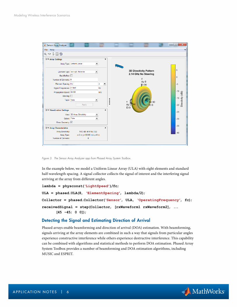
Phased Array System Toolbox provides algorithms and apps for the design, simulation, and analysis of phased arrays. For example, the Sensor Array Analyzer app lets you examine important properties of a phased array such as shape and directivity (Figure 3). You can design the array interactively, and then generate MATLAB code to use the array in simulations.



Figure 3. The Sensor Array Analyzer app from Phased Array System Toolbox.

In the example below, we model a Uniform Linear Array (ULA) with eight elements and standard half-wavelength spacing. A signal collector collects the signal of interest and the interfering signal arriving at the array from different angles.

lambda = physconst(‘LightSpeed’)/fc;

ULA = phased.ULA(8, ‘ElementSpacing’, lambda/2);

Collector = phased.Collector(‘Sensor’, ULA, ‘OperatingFrequency’, fc);

receivedSignal = step(Collector, [rxWaveform1 rxWaveform2], ... [45 -45; 0 0]);

Detecting the Signal and Estimating Direction of Arrival

Phased arrays enable beamforming and direction of arrival (DOA) estimation. With beamforming, signals arriving at the array elements are combined in such a way that signals from particular angles experience constructive interference while others experience destructive interference. This capability can be combined with algorithms and statistical methods to perform DOA estimation. Phased Array System Toolbox provides a number of beamforming and DOA estimation algorithms, including MUSIC and ESPRIT.



In this example, we use a statistical test (the Akaike information criterion) to estimate the number of signals impinging on the array elements. We then use a beamscan estimation algorithm to scan the array beam through a range of angles and identify the angles at which the received signal power is highest. These angles represent the estimated direction of arrival of the signal of interest and the interfering signal.

numSignals = aictest(awgn(receivedSignal*10000, 40));

Beamscan = phased.BeamscanEstimator(‘SensorArray’, ULA, ... ‘OperatingFrequency’, fc, ‘DOAOutputPort’, true, ... ‘NumSignals’, numSignals, ‘ScanAngles’, -90:90);

[~, doas] = step(Beamscan, receivedSignal)

doas =

45 -45

Beamforming and Performing a Cell Search

Once the angles of arrival have been identified, we use beamforming to spatially isolate each signal. We steer the array beam to each identified angle, receive the signal, and perform receiver signal processing.

Beamforming is performed by computing weights by which to multiply the signal received at each array element. The received signal is multiplied by the weights to emphasize the signal received from the desired angle and minimize the signal received from the undesired angle (null steering).

The lteCellSearch function in LTE System Toolbox performs a cell search on a received signal, identifying cells present based on the peak magnitude of correlations with the primary and secondary synchronization signals. In this case, we identify the most powerful cell received from each angle based on the cell’s Reference Signal Received Power (RSRP). RSRP is one of the metrics used by a mobile unit to select which cell to communicate with. The demodulateLTESignal function identi-fies the beginning of the LTE frame, computes the RSRP, estimates the channel response and per-forms equalization, and performs deprecoding, layer demapping, demodulation, and descrambling on the received data. The end result is the estimate of the received bits.

for ii = 1:length(doas)

% Use beamforming to steer beam to angle of arriving signal

w(:,ii) = sidelobeCanceller(ULA.getElementPosition/lambda, ... doas(ii), setdiff(doas, doas(ii)));

ybf(:,ii) = receivedSignal * conj(w(:,ii));

% Identify the most powerful cell received from this angle

searchalg.MaxCellCount = 1;

searchalg.SSSDetection = ‘PostFFT’;



[cellIDs(ii), ~] = lteCellSearch(enb1, ybf(:,ii), searchalg);

% Perform LTE demodulation and RSRP measurement on beamformed signal

try [rxData(:,ii) rxRSRPs(ii), rxSymbols(:,ii)] = ... demodulateLTESignal(enb1, ybf(:,ii));

catch, end

end

% Compute result without beamforming (for comparison later)

y = sum(receivedSignal,2);

rxNoBF = demodulateLTESignal(enb1, y);

Selecting the Signal of Interest

Now that we have identified the signals present and their angles of arrival, we can select the signal of interest based on its angle. Here, we simply select the angle closest to our desired angle of 45 degrees. We use a polar plot to display the array pattern and angles of arrival of the signals we’ve identified (Figure 4).

[~, signalSelect] = min(abs(doas - 45));

rxData = rxData(:,signalSelect);

Figure 4. A polar plot showing the array pattern and identified signals with angles of arrival.



Visualizing Signals

Using scopes provided by Communications System Toolbox and DSP System Toolbox™, we plot the received symbol constellation of the signal of interest after beamforming (Figure 5) and the received spectrum of each signal (Figure 6).

Constellation = ... comm.ConstellationDiagram(‘ShowReferenceConstellation’, ... false, ‘ShowGrid’, true);

step(Constellation, rxSymbols(:,signalSelect));

SpectrumAnalyzer = dsp.SpectrumAnalyzer(‘SampleRate’, 15360000, ‘SpectralAverages’, 1, ... ‘PowerUnits’, ‘dBW’, ‘PlotAsTwoSidedSpectrum’, true, ‘Name’, ... ‘Received Signals at UE’, ‘ChannelNames’, {‘SOI’, ‘Interferer’}, ... ‘ShowLegend’ , true);

step(SpectrumAnalyzer, [rxWaveform1 rxWaveform2]);

Figure 5. A constellation diagram of the signal of interest.


A P P L I C AT I O N N O T E S | 1 0

Figure 6. Received spectrum of the signal of interest and the interferer.

Evaluating System Performance

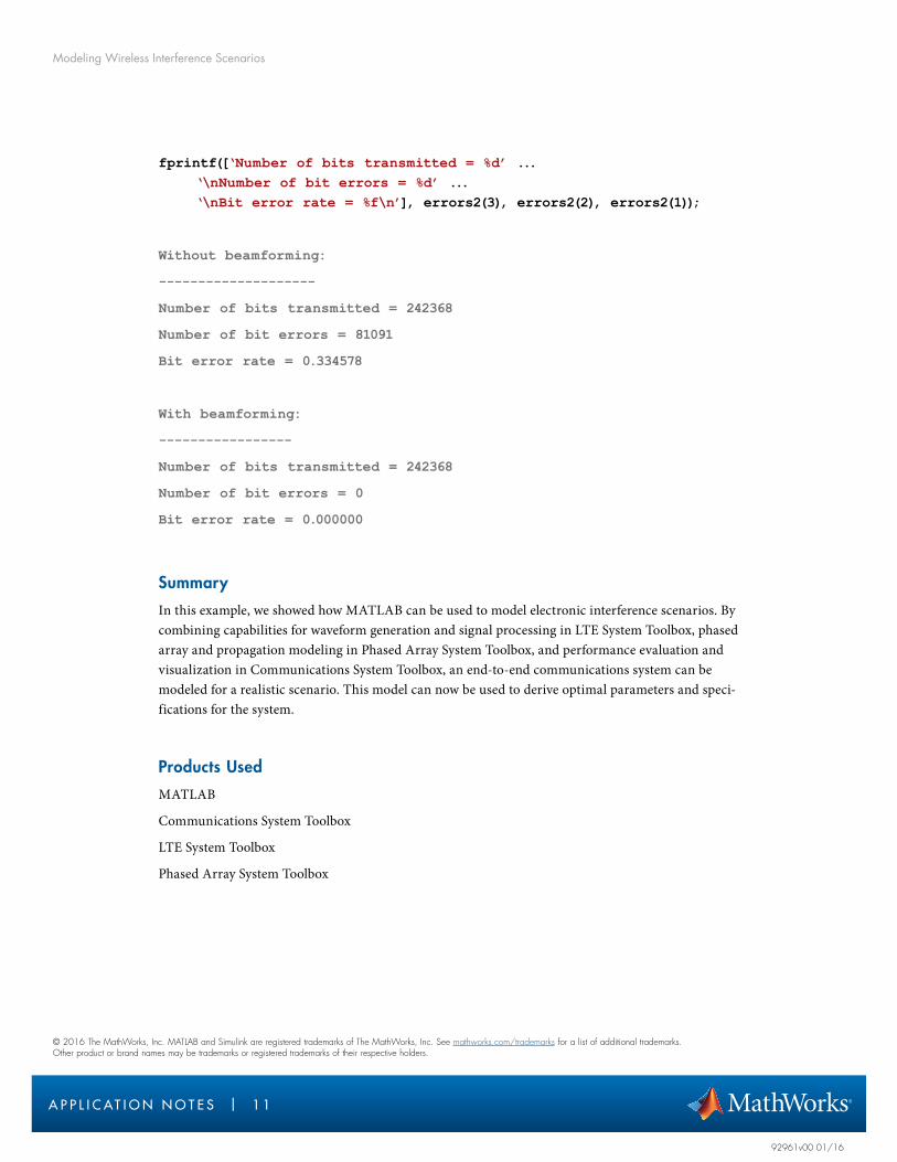
A key performance metric of a digital communications systems is the Bit Error Rate (BER), or the percentage of bits which are received in error. We use a System object from Communications System Toolbox to compute the BER. We use the BER metric to quantify the effect of beamforming in improving system performance.

fprintf(‘\nWithout beamforming:\n--------------------\n’);

BER1=comm.ErrorRate;

errors1 = step(BER1, double(rxNoBF), data1(1:length(rxNoBF)));

fprintf([‘Number of bits transmitted = %d’ ... ‘\nNumber of bit errors = %d’ ... ‘\nBit error rate = %f\n’], errors1(3), errors1(2), errors1(1));

fprintf(‘\nWith beamforming:\n-----------------\n’);

BER2=comm.ErrorRate;

errors2 = step(BER2, double(rxData), data1(1:length(rxData)));


A P P L I C AT I O N N O T E S | 1 1

© 2016 The MathWorks, Inc. MATLAB and Simulink are registered trademarks of The MathWorks, Inc. See mathworks.com/trademarks for a list of additional trademarks. Other product or brand names may be trademarks or registered trademarks of their respective holders.

92961v00 01/16

fprintf([‘Number of bits transmitted = %d’ ... ‘\nNumber of bit errors = %d’ ... ‘\nBit error rate = %f\n’], errors2(3), errors2(2), errors2(1));

Without beamforming:

--------------------

Number of bits transmitted = 242368

Number of bit errors = 81091

Bit error rate = 0.334578

With beamforming:

-----------------

Number of bits transmitted = 242368

Number of bit errors = 0

Bit error rate = 0.000000

Summary

In this example, we showed how MATLAB can be used to model electronic interference scenarios. By combining capabilities for waveform generation and signal processing in LTE System Toolbox, phased array and propagation modeling in Phased Array System Toolbox, and performance evaluation and visualization in Communications System Toolbox, an end-to-end communications system can be modeled for a realistic scenario. This model can now be used to derive optimal parameters and speci-fications for the system.

Products Used

MATLAB

Communications System Toolbox

LTE System Toolbox

Phased Array System Toolbox

http://www.mathworks.com/trademarks

modeling wireless interference scenarios - mathworks wireless interference scenarios ... this...

Documents