modeling with observational data michael babyak, phd
TRANSCRIPT
Modeling with Observational Data
Michael Babyak, PhD
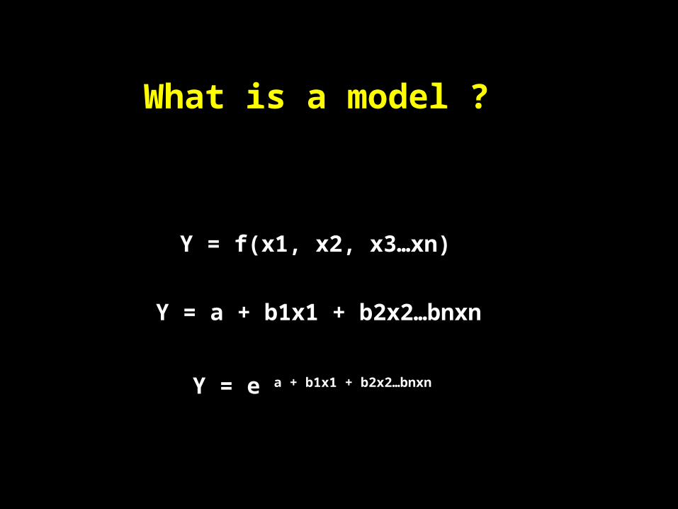
What is a model ?
Y = f(x1, x2, x3…xn)
Y = a + b1x1 + b2x2…bnxn
Y = e a + b1x1 + b2x2…bnxn
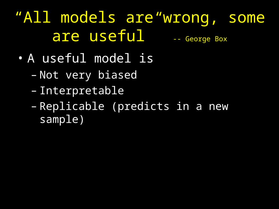
“All models are wrong, some are useful” -- George Box
• A useful model is– Not very biased– Interpretable– Replicable (predicts in a new sample)
Some Premises
• “Statistics” is a cumulative, evolving field• Newer is not necessarily better, but should be
entertained in the context of the scientific question at hand
• Data analytic practice resides along a continuum, from exploratory to confirmatory. Both are important, but the difference has to be recognized.
• There’s no substitute for thinking about the problem
Observational Studies
• Underserved reputation
• Especially if conducted and analyzed ‘wisely’
• Biggest threats– “Third Variable”– Selection Bias (see above)– Poor Planning

Correlation between results of randomized trials and observational studies
http://www.epidemiologic.org/2006/11/agreement-of-observational-and.html

-1.0 -0.5 0.0 0.5 1.0 1.5 2.0
-1.5
-1.0
-0.5
0.0
0.5
1.0
1.5
Bland-Altman difference plot
Mean
Diff
eren
ce
Mean of Estimates
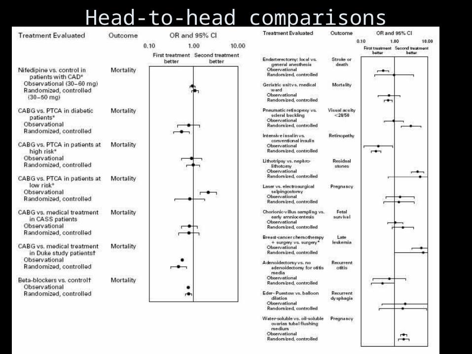
Head-to-head comparisons

Statistics is a cumulative, evolving field: How do we know this stuff?
• Theory
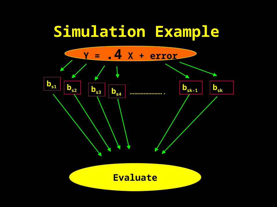
• Simulation

Y = b X + error
bs
1
bs
2
bs
3
bs
4
bsk-1 bsk………………….
Concept of Simulation

bs
1
bs
2
bs
3
bs
4
bsk-1 bsk………………….
Y = b X + error
Evaluate
Concept of Simulation

Y = .4 X + error
bs
1
bs
2
bs
3
bs
4
bsk-1 bsk………………….
Simulation Example
bs
1
bs
2
bs
3
bs
4
bsk-1 bsk………………….
Evaluate
Y = .4 X + error
Simulation Example

0.2 0.4 0.6
05
00
10
00
15
00
20
00
25
00
Value of beta for x1
Fre
qu
en
cy o
f b
eta
va
lue
True Model:Y = .4*x1 + e
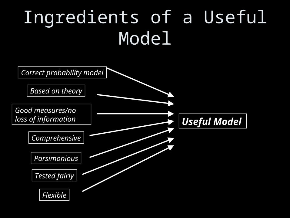
Ingredients of a Useful Model
Correct probability model
Good measures/no loss of information
Based on theory
Comprehensive
Parsimonious
Flexible
Tested fairly
Useful Model

Correct Model
• Gaussian: General Linear Model• Multiple linear regression
• Binary (or ordinal): Generalized Linear Model• Logistic Regression• Proportional Odds/Ordinal Logistic
• Time to event: • Cox Regression or parametric survival
models
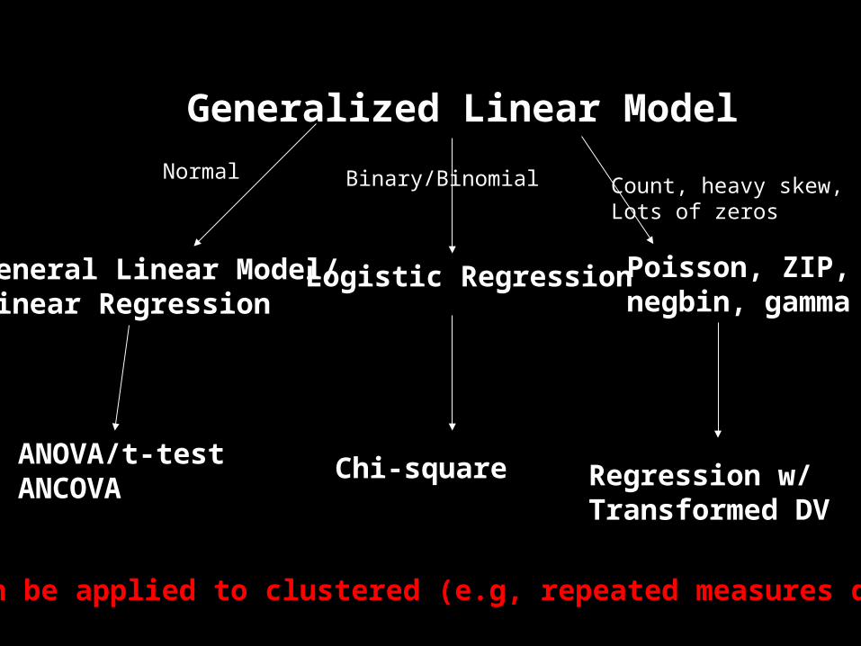
Generalized Linear Model
General Linear Model/Linear Regression
ANOVA/t-testANCOVA
Logistic Regression
Chi-square
Poisson, ZIP,negbin, gamma
Normal Binary/Binomial Count, heavy skew,Lots of zeros
Regression w/Transformed DV
Can be applied to clustered (e.g, repeated measures data)

Factor Analytic Family
Structural Equation Models
Partial Least SquaresLatent Variable Models
(Confirmatory Factor Analysis)
Multiple regression Principal
Components
Common FactorAnalysis
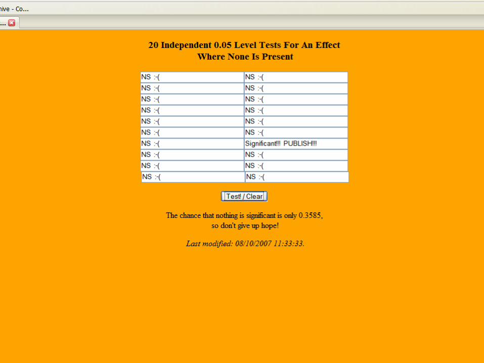
Use Theory
• Theory and expert information are critical in helping sift out artifact
• Numbers can look very systematic when the are in fact random– http://www.tufts.edu/~gdallal/multtest.htm


Measure well
Adequate rangeRepresentative valuesWatch for ceiling/floor effects
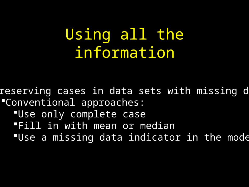
Using all the information
Preserving cases in data sets with missing dataConventional approaches:
Use only complete caseFill in with mean or medianUse a missing data indicator in the model
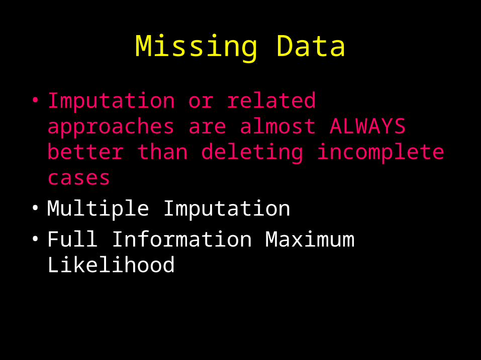
Missing Data
• Imputation or related approaches are almost ALWAYS better than deleting incomplete cases
• Multiple Imputation
• Full Information Maximum Likelihood
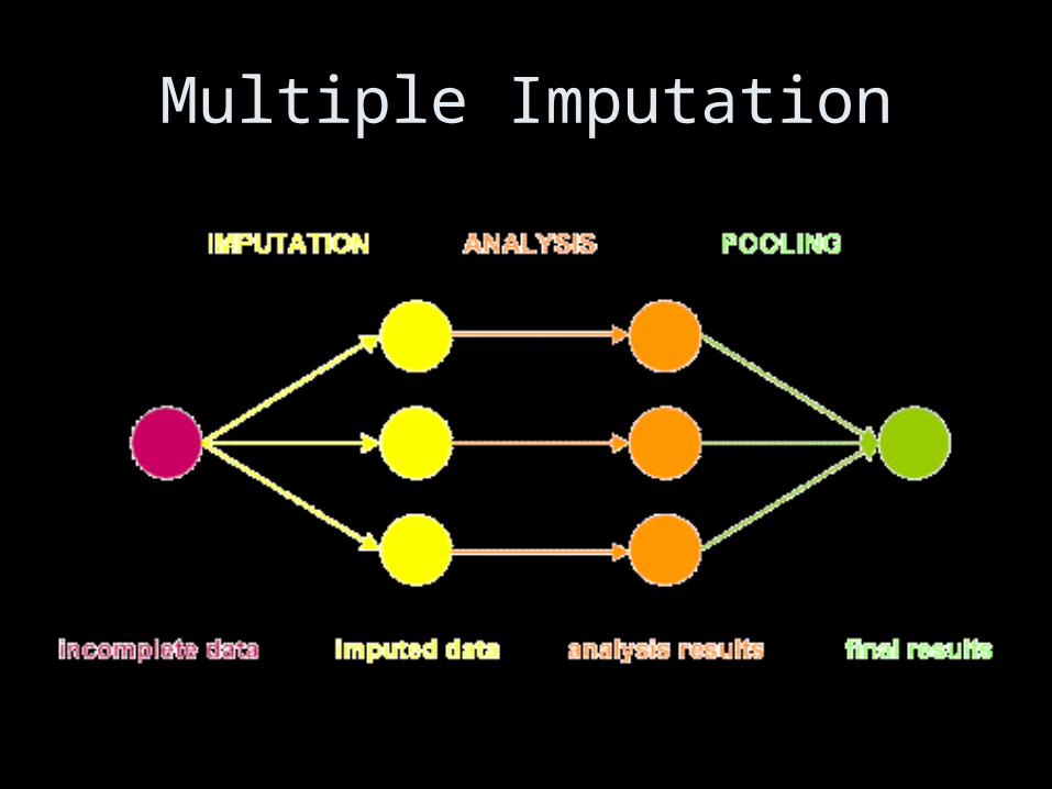
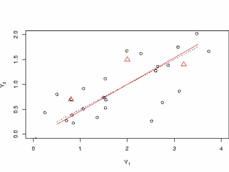
Multiple Imputation

http://www.lshtm.ac.uk/msu/missingdata/mi_web/node5.html
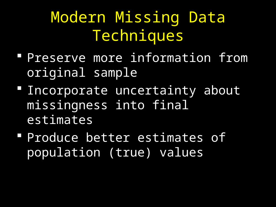
Modern Missing Data Techniques
Preserve more information from original sample
Incorporate uncertainty about missingness into final estimates
Produce better estimates of population (true) values

Don’t waste information from variables
• Use all the information about the variables of interest
• Don’t create “clinical cutpoints” before modeling
• Model with ALL the data first, then use prediction to make decisions about cutpoints

Dichotomizing for Convenience = Dubious Practice
(C.R.A.P.*)
•Convoluted Reasoning and Anti-intellectual Pomposity •Streiner & Norman: Biostatistics: The Bare Essentials
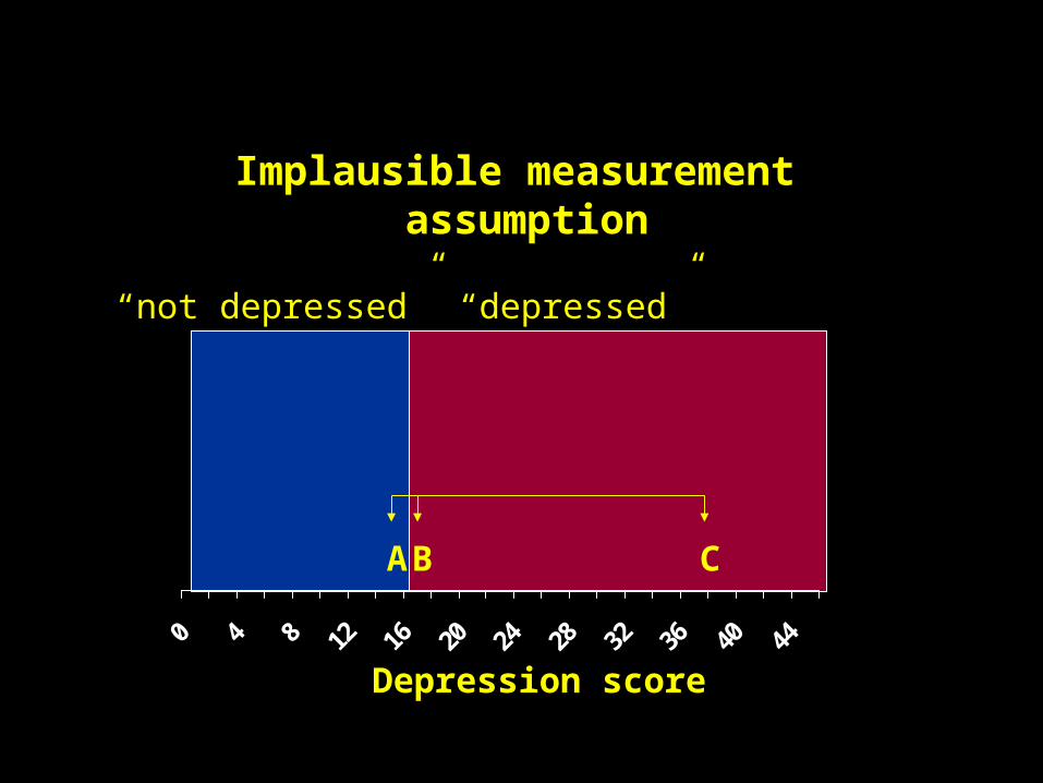
0 4 8 12 16 20 24 28 32 36 40 44
Depression score
AB C
Implausible measurement assumption
“not depressed” “depressed”

http://psych.colorado.edu/~mcclella/MedianSplit/
http://www.bolderstats.com/jmsl/doc/medianSplit.html
Loss of power
Sometimes through sampling errorYou can get a ‘lucky cut.’

Dichotomization, by definition, reduces the magnitude of the estimate
by a minimum of about 30%
Dear Project Officer,
In order to facilitate analysis and interpretation, we have decided to throw away about 30% of our data. Even though this will waste about 3 or 4 hundred thousand dollars worth of subject recruitment and testing money, we are confident that you will understand.
Sincerely,
Dick O. Tomi, PhDProf. Richard Obediah Tomi, PhD

Power to detect non-zero b-weight when x is continuous versus
dichotomized
50
60
70
80
90
100
0.85 0.75 0.65Reliability of x
% c
orr
ec
t re
jec
tio
ns
of
nu
ll h
yp
oth
es
is
Continuous xDichotomized x
True model: y =.4x + e
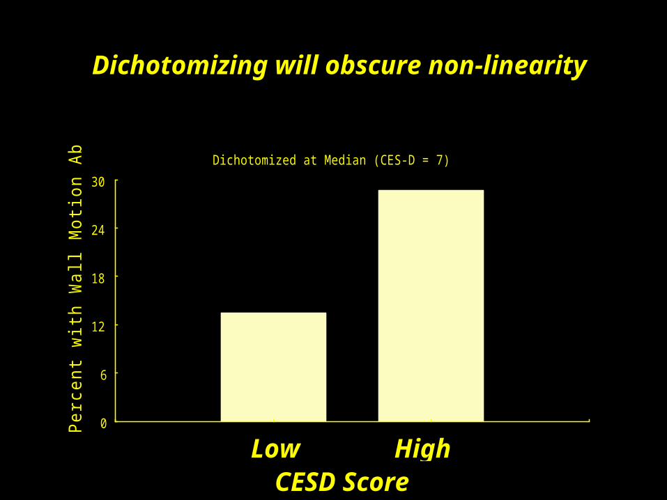
Dichotomizing will obscure non-linearity
Dichotomized at Median (CES-D = 7)
Perc
ent w
ith W
all
Motio
n A
bnorm
alit
y
0
6
12
18
24
30
Not Depressed Depressed
Low HighCESD Score
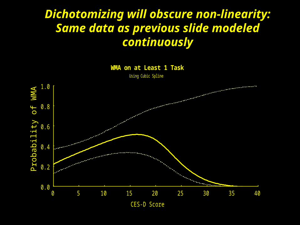
WMA on at Least 1 TaskUsing Cubic Spline
CES-D Score
Pro
babi
lity
of W
MA
0.0
0.2
0.4
0.6
0.8
1.0
0 5 10 15 20 25 30 35 40
Dichotomizing will obscure non-linearity:Same data as previous slide modeled
continuously
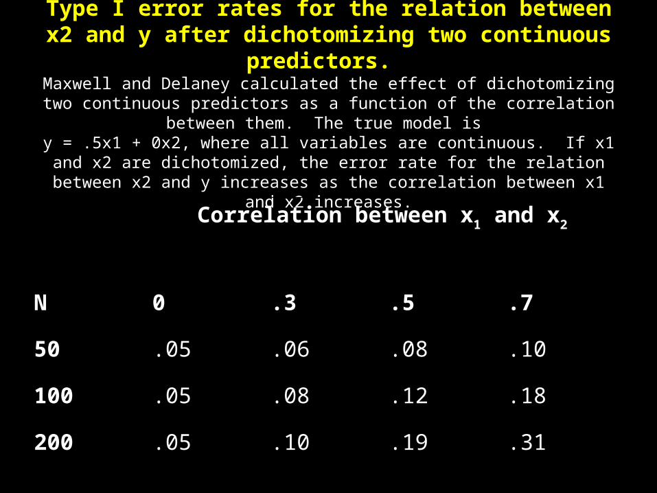
Type I error rates for the relation between x2 and y after dichotomizing two continuous predictors.
Maxwell and Delaney calculated the effect of dichotomizing two continuous predictors as a function of the correlation between them. The true model is
y = .5x1 + 0x2, where all variables are continuous. If x1 and x2 are dichotomized, the error rate for the relation between x2 and y increases as the
correlation between x1 and x2 increases.
Correlation between x1 and x2
N 0 .3 .5 .7
50 .05 .06 .08 .10
100 .05 .08 .12 .18
200 .05 .10 .19 .31
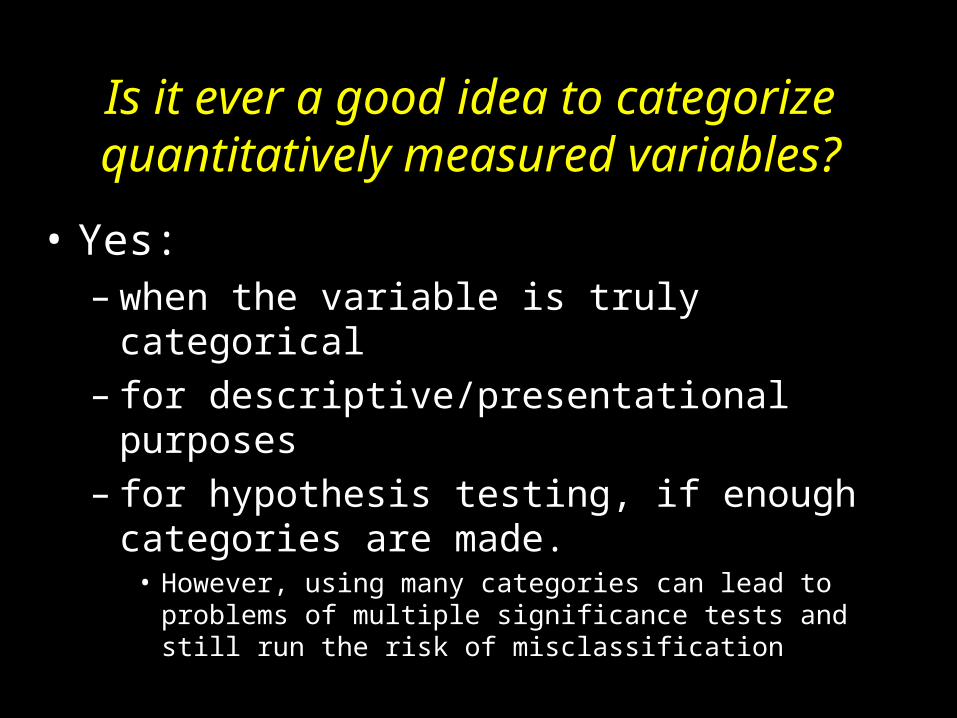
Is it ever a good idea to categorize quantitatively measured variables?
• Yes: – when the variable is truly categorical– for descriptive/presentational purposes– for hypothesis testing, if enough categories
are made.• However, using many categories can lead to problems of
multiple significance tests and still run the risk of misclassification
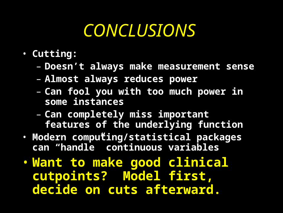
CONCLUSIONS• Cutting:
– Doesn’t always make measurement sense– Almost always reduces power– Can fool you with too much power in some
instances– Can completely miss important features of the
underlying function• Modern computing/statistical packages can
“handle” continuous variables
• Want to make good clinical cutpoints? Model first, decide on cuts afterward.
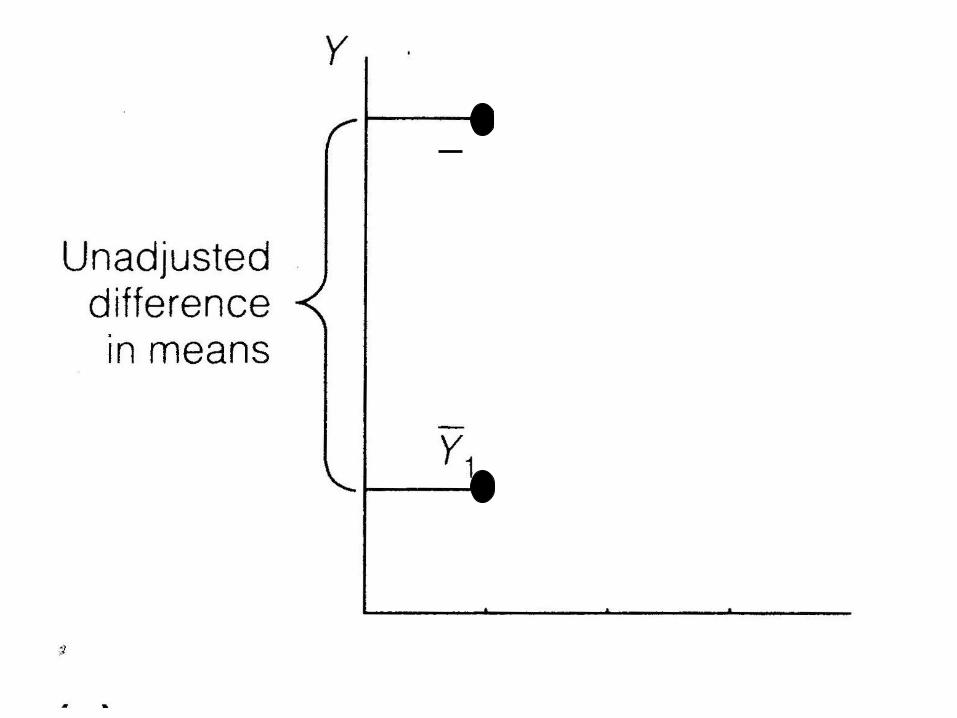
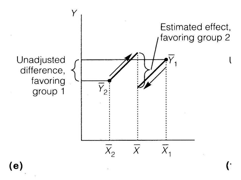
Statistical Adjustment/Control
• What does it mean to ‘adjust’ or ‘control’ for another variable?
Y 2
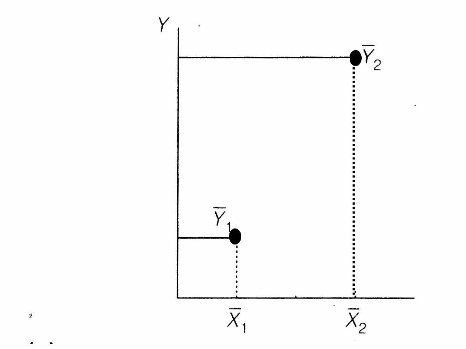
Covariate X

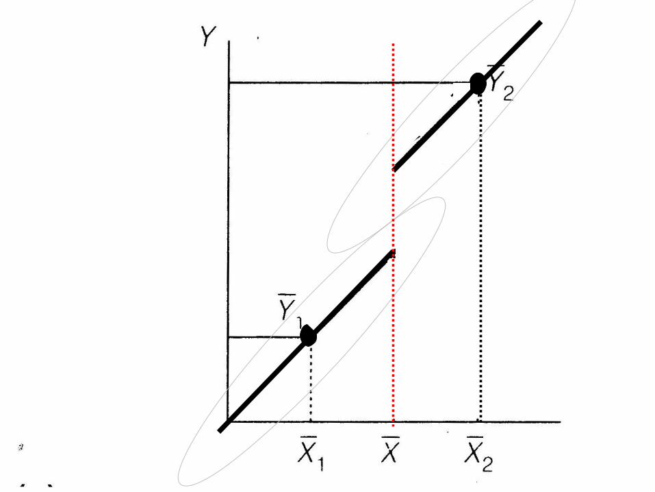

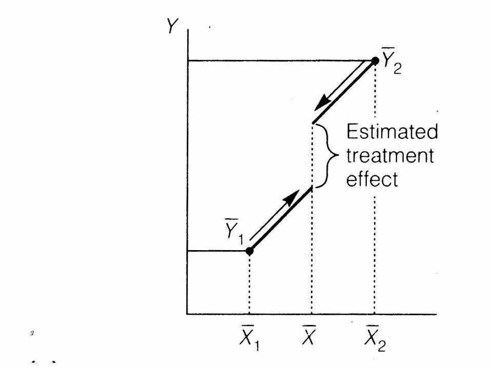


Y
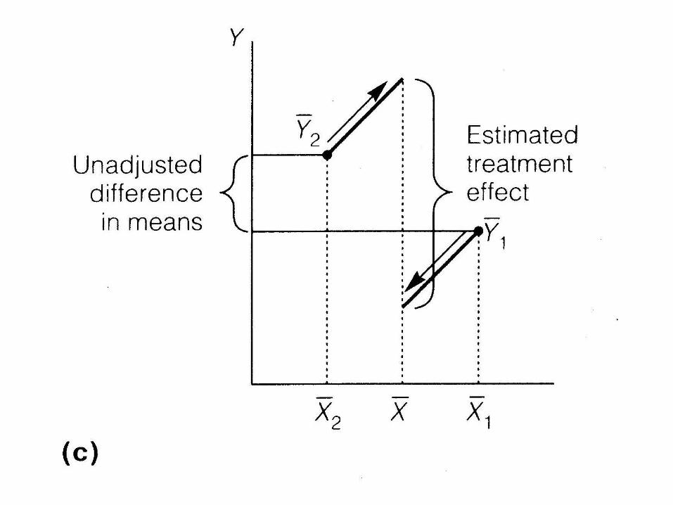
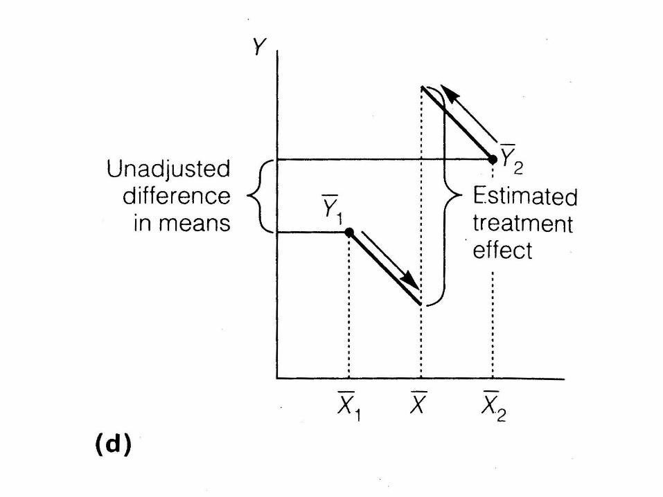

Difficulties
• What if lines aren’t parallel?
• What if poor overlap between groups?

A Note on Mediation vs Confounding
• Mathematically identical– no test can tell you which is which
• Depends on YOUR causal hypothesis
• Criteria for either:– All three variables, predictor,
confounder/mediator, outcome must be related
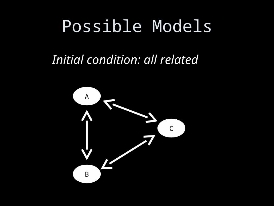
Possible Models
A
B
C
Initial condition: all related
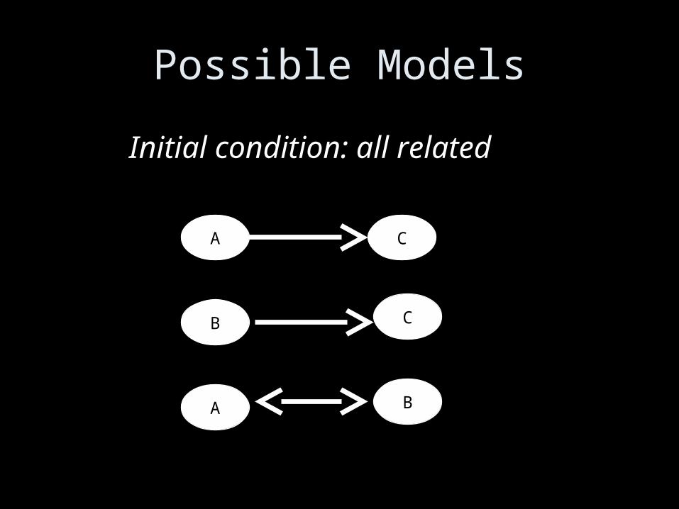
Possible Models
A
B
C
Initial condition: all related
C
A B
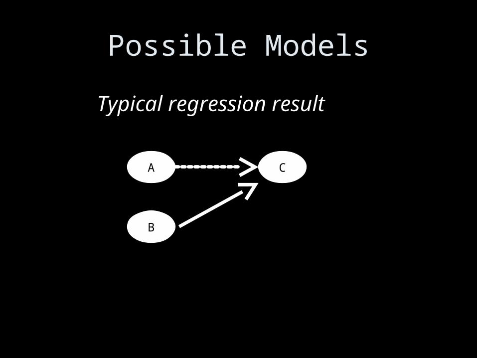
Possible Models
A
B
C
Typical regression result
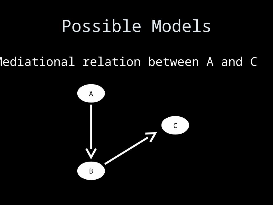
Possible Models
A
B
C
Mediational relation between A and C

Possible Models
A
B
C
Spurious relation between A and C

Possible Models
A
B
C
Or worse
U

• With cross-sectional design, best you can do is say that observed relations are consistent/not consistent with hypothesized relation
• Prospective better but still vulnerable to outside variables
• Interpretation of mediator/confounding distinction is entirely substantive
Not always clear difference between mediator and confounder
• Beware that adjustment for confounder might actually be modeling an explanatory mechanism
• E.g., relation between depression and mortality
• Often adjust for medical comorbidity• Comorbidity however, might be a proxy for
poor self-care, which in turn is linked to depression
Sample size and the problem of underfitting vs overfitting
• Model assumption is that “ALL” relevant variables be included—the “antiparsimony principle” or “As big as a house.”
• Tempered by fact that estimating too many unknowns with too little data will yield junk.
• In other words, can’t build a mansion with a shanty’s worth of wood.
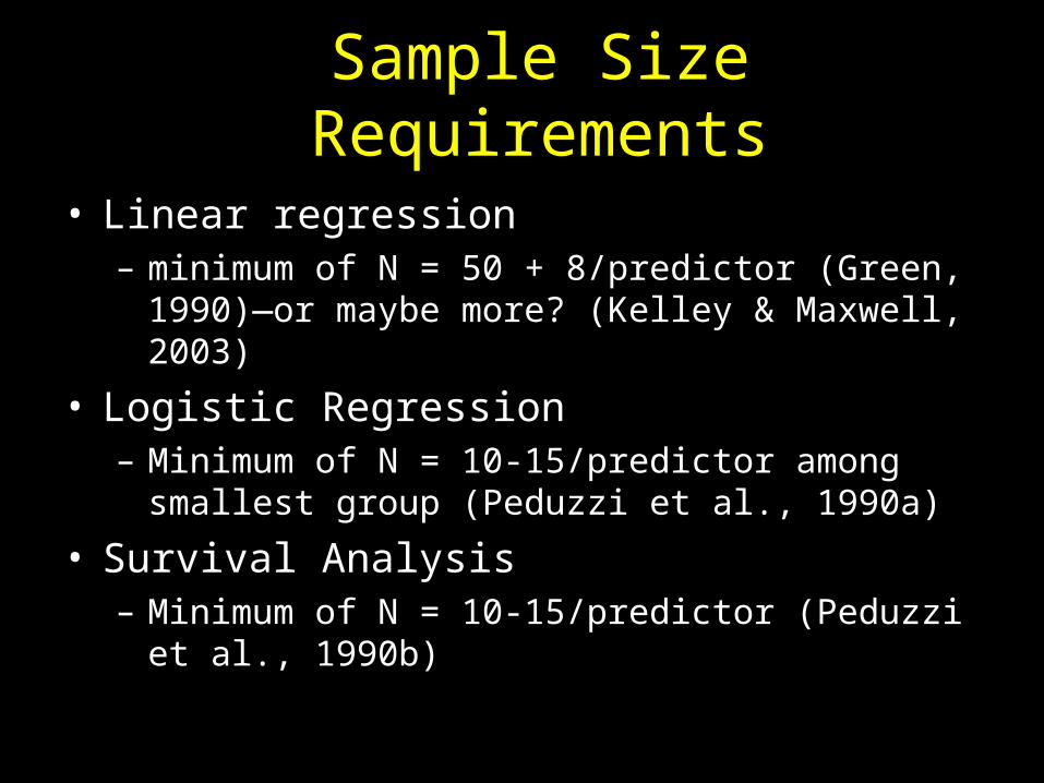
Sample Size Requirements• Linear regression
– minimum of N = 50 + 8/predictor (Green, 1990)—or maybe more? (Kelley & Maxwell, 2003)
• Logistic Regression– Minimum of N = 10-15/predictor among smallest
group (Peduzzi et al., 1990a)
• Survival Analysis– Minimum of N = 10-15/predictor (Peduzzi et al.,
1990b)

Consequences of inadequate sample size
• Lack of power for individual tests
• Unstable estimates
• Spurious good fit—lots of unstable estimates will produce spurious ‘good-looking’ (big) regression coefficients

All-noise, but good fit
R-Square from Full Model
De
nsi
ty
0.0 0.1 0.2 0.3 0.4 0.5 0.6 0.7 0.8 0.9 1.0
02
46
81
01
21
41
6
n/p~3n/p~6.6n/p=10n/p~13.3
Events per predictor ratio
R-squares from multivariable models where population is completely random numbers
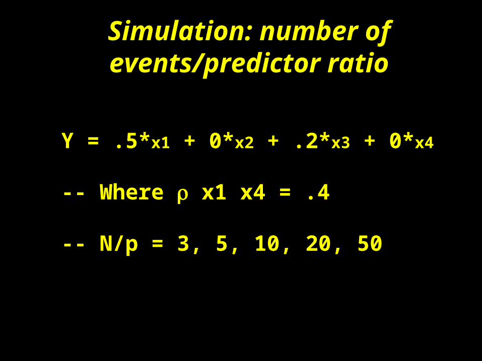
Simulation: number of events/predictor ratio
Y = .5*x1 + 0*x2 + .2*x3 + 0*x4
-- Where x1 x4 = .4
-- N/p = 3, 5, 10, 20, 50
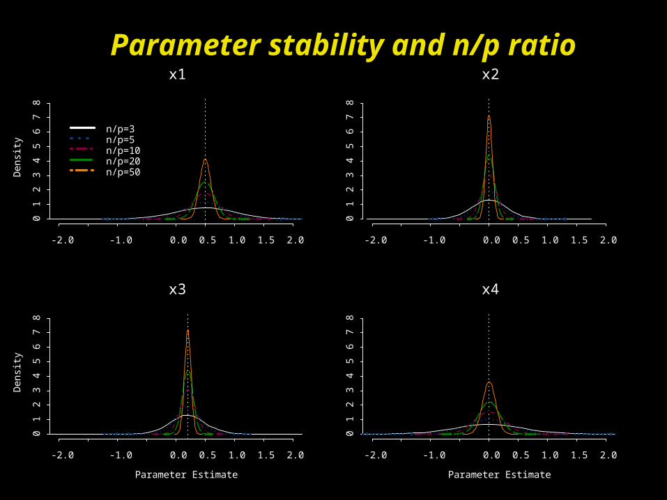
Parameter stability and n/p ratiox1
Den
sity
-2.0 -1.0 0.0 0.5 1.0 1.5 2.0
01
23
45
67
8
n/p=3n/p=5n/p=10n/p=20n/p=50
x2
-2.0 -1.0 0.0 0.5 1.0 1.5 2.0
01
23
45
67
8
x3
Parameter Estimate
Den
sity
-2.0 -1.0 0.0 0.5 1.0 1.5 2.0
01
23
45
67
8
x4
Parameter Estimate
-2.0 -1.0 0.0 0.5 1.0 1.5 2.0
01
23
45
67
8
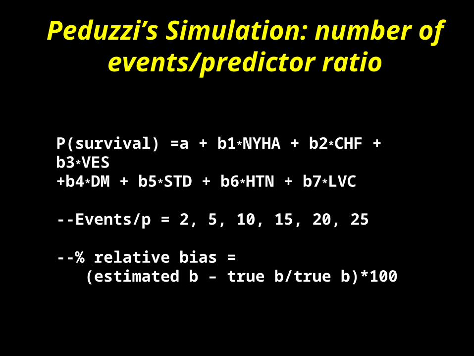
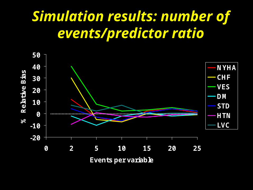
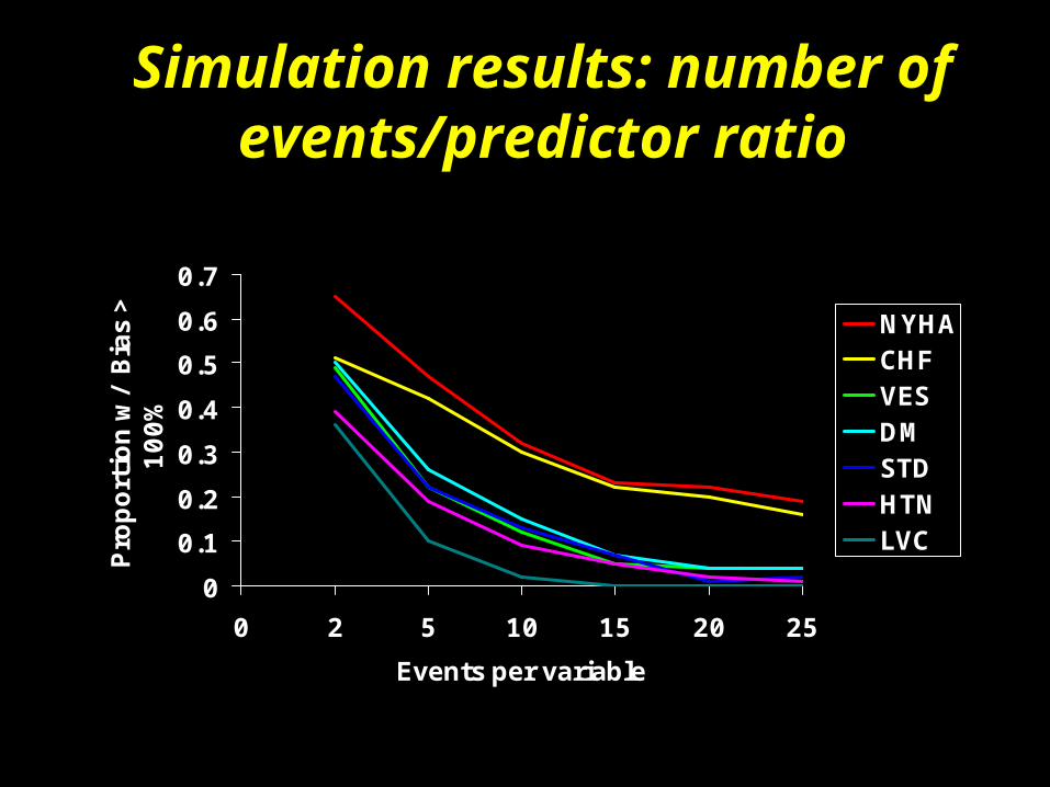
Peduzzi’s Simulation: number of events/predictor ratio
P(survival) =a + b1*NYHA + b2*CHF + b3*VES+b4*DM + b5*STD + b6*HTN + b7*LVC
--Events/p = 2, 5, 10, 15, 20, 25
--% relative bias = (estimated b – true b/true b)*100
-20
-10
0
10
20
30
40
50
0 2 5 10 15 20 25
Events per variable
% R
elat
ive
Bia
s NYHACHFVESDMSTDHTNLVC
Simulation results: number of events/predictor ratio
0
0.1
0.2
0.3
0.4
0.5
0.6
0.7
0 2 5 10 15 20 25
Events per variable
Pro
port
ion w
/ B
ias
>
100%
NYHACHFVESDMSTDHTNLVC
Simulation results: number of events/predictor ratio

Approaches to variable selection
• “Stepwise” automated selection• Pre-screening using univariate tests• Combining or eliminating redundant predictors• Fixing some coefficients• Theory, expert opinion and experience• Penalization/Random effects• Propensity Scoring
– “Matches” individuals on multiple dimensions to improve “baseline balance”
• Tibshirani’s “Lasso”

Any variable selection technique based on looking at the data first
will likely be biased

“I now wish I had never written the stepwise selection code for SAS.” --Frank Harrell, author of forward and
backwards selection algorithm for SAS PROC REG
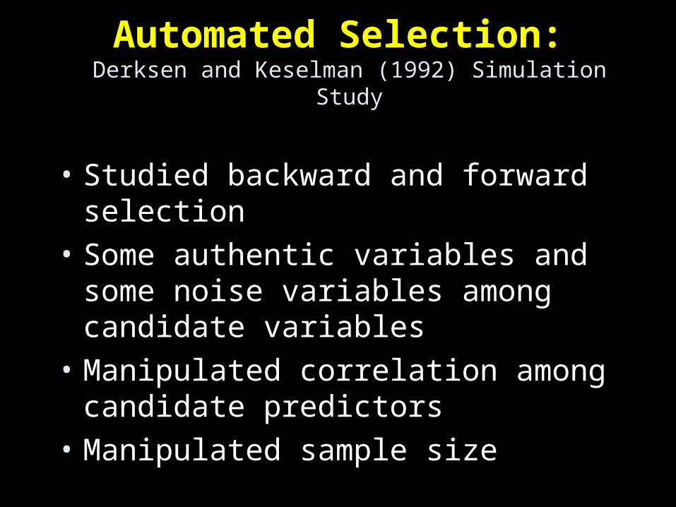
Automated Selection: Derksen and Keselman (1992) Simulation Study
• Studied backward and forward selection
• Some authentic variables and some noise variables among candidate variables
• Manipulated correlation among candidate predictors
• Manipulated sample size
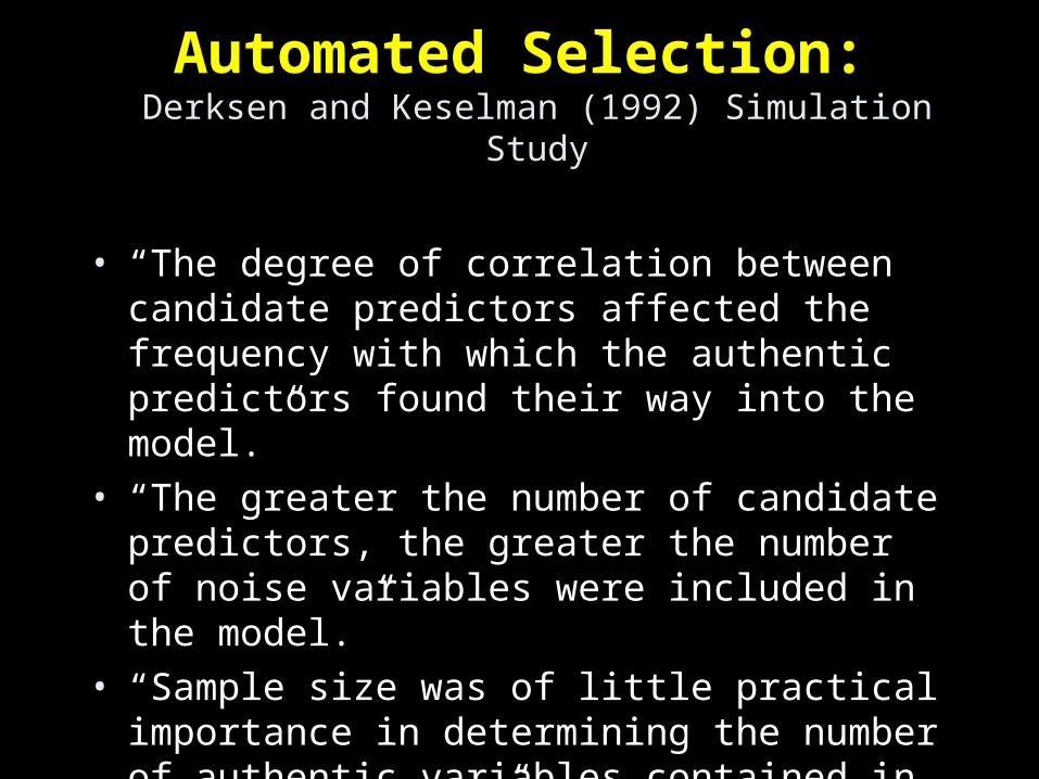
Automated Selection: Derksen and Keselman (1992) Simulation Study
• “The degree of correlation between candidate predictors affected the frequency with which the authentic predictors found their way into the model.”
• “The greater the number of candidate predictors, the greater the number of noise variables were included in the model.”
• “Sample size was of little practical importance in determining the number of authentic variables contained in the final model.”

0
5
10
15
20
25
30
35
0 1 2 3 4 5 6 7
Variables in Final Model
% o
f sa
mple
s
100200500100010000
Simulation results: Number of noise variables included
20 candidate predictors; 100 samples
Sample Size
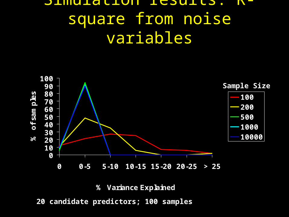
0102030405060708090
100
0 0-5 5-10 10-15 15-20 20-25 > 25
% Variance Explained
% o
f sa
mple
s
100200500100010000
Simulation results: R-square from noise variables
20 candidate predictors; 100 samples
Sample Size
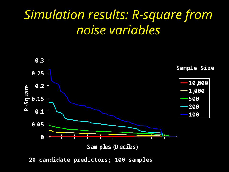
0
0.05
0.1
0.15
0.2
0.25
0.3
Samples (Deciles)
R-S
quare
10,0001,000500200100
Simulation results: R-square from noise variables
20 candidate predictors; 100 samples
Sample Size
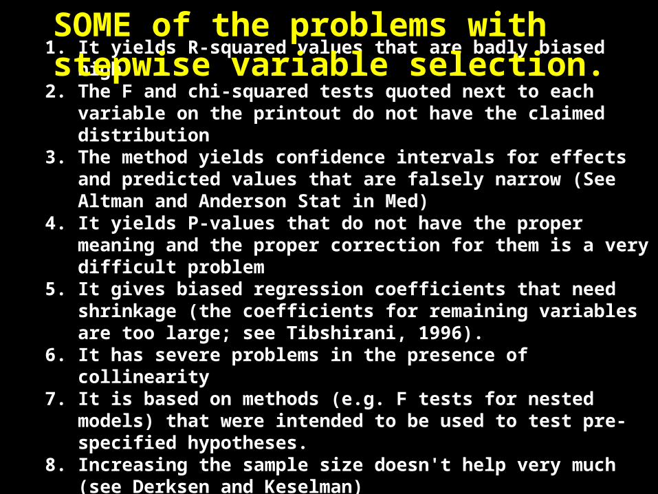
1. It yields R-squared values that are badly biased high 2. The F and chi-squared tests quoted next to each variable on the
printout do not have the claimed distribution 3. The method yields confidence intervals for effects and predicted
values that are falsely narrow (See Altman and Anderson Stat in Med)
4. It yields P-values that do not have the proper meaning and the proper correction for them is a very difficult problem
5. It gives biased regression coefficients that need shrinkage (the coefficients for remaining variables are too large; see Tibshirani, 1996).
6. It has severe problems in the presence of collinearity 7. It is based on methods (e.g. F tests for nested models) that were
intended to be used to test pre-specified hypotheses. 8. Increasing the sample size doesn't help very much (see Derksen
and Keselman) 9. It allows us to not think about the problem 10. It uses a lot of paper
SOME of the problems with stepwise variable selection.

author ={Chatfield, C.}, title = {Model uncertainty, data mining and statistical inference (with discussion)}, journal = JRSSA, year = 1995, volume = 158, pages = {419-466}, annote =
--bias by selecting model because it fits the data well; bias in standard errors; P. 420: ... need for a better balance in the literature and in statistical teaching between techniques and problem solving strategies}. P. 421: It is `well known' to be `logically unsound and practically misleading' (Zhang, 1992) to make inferences as if a model is known to be true when it has, in fact, been selected from the same data to be used for estimation purposes. However, although statisticians may admit this privately (Breiman (1992) calls it a `quiet scandal'), they (we) continue to ignore the difficulties because it is not clear what else could or should be done. P. 421: Estimation errors for regression coefficients are usually smaller than errors from failing to take into account model specification. P. 422: Statisticians must stop pretending that model uncertainty does not exist and begin to find ways of coping with it. P. 426: It is indeed strange that we often admit model uncertainty by searching for a best model but then ignore this uncertainty by making inferences and predictions as if certain that the best fitting model is actually true.
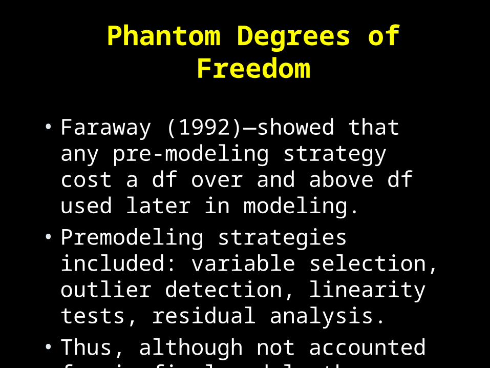
Phantom Degrees of Freedom
• Faraway (1992)—showed that any pre-modeling strategy cost a df over and above df used later in modeling.
• Premodeling strategies included: variable selection, outlier detection, linearity tests, residual analysis.
• Thus, although not accounted for in final model, these phantom df will render the model too optimistic

Phantom Degrees of Freedom
• Therefore, if you transform, select, etc., you must include the DF in (i.e., penalize for) the “Final Model”

Conventional Univariate Pre-selection
• Non-significant tests also cost a DF• Non-significance is NOT
necessarily related to importance• Variables may not behave the
same way in a multivariable model—variable “not significant” at univariate test may be very important in the presence of other variables

• Despite the convention, testing for confounding has not been systematically studied—in many cases leads to overadjustment and underestimate of true effect of variable of interest.
• At the very least, pulling variables in and out of models inflates the model fit, often dramatically
Conventional Univariate Pre-selection

Better approach
• Pick variables a priori• Stick with them• Penalize appropriately for any
data-driven decision about how to model a variable

Spending DF wisely
• If not enough N/predictor, combine covariates using techniques that do not look at Y in the sample, PCA, FA, conceptual clustering, collapsing, scoring, established indexes.
• Save DF for finer-grained look at variables of most interest, e.g, non-linear functions

What to do
• Penalization/Random effects
• Propensity Scoring– “Matches” individuals on multiple dimensions
to improve “baseline balance”
• Tibshirani’s Lasso

Canadian Study UK Study US StudyNo Smoke Cig. Cig./Pipe No Smoke Cig. Cig./Pipe No Smoke Cig. Cig./ Pipe
A Death Rates per 1,000 Person Years
20.2 20.5 35.5 11.3 14.1 20.7 13.5 13.5 17.4
B Average Age in Years
54.9 50.5 65.9 49.1 49.8 55.7 57.0 53.2 59.7
C Adjusted Death Rates Using K Subclasses
K=2 20.2 26.4 24.0 11.3 12.7 13.6 13.5 16.4 14.9
K=3 20.2 28.3 21.2 11.3 12.8 12.0 13.5 17.7 14.2
K=9-11
20.2 29.5 19.8 11.3 14.8 11.0 13.5 21.2 13.7

Propensity Score Example
• Observational data on SSRI use in post myocardial infarction patients
• Early use of SSRI as an adjustment covariate revealed excess risk for all-cause mortality among SSRI users
• Can use Propensity Score to help rule out confounders

Step 1: “Kitchen Sink” Model predicting SSRI use
• Why is it OK to use lots of predictors in this case?
• Working strictly at the sample level

Odds Ratio
0.50 1.50 2.50 3.50 4.50 5.50 6.50
age - 70:53male - 1:0white - 1:0
bmi - 33:26diabetes - 1:0
htn - 1:0famhx - 1:0copd - 1:0
pvd - 1:0cvd - 1:0
esrd - 1:0mihx - 1:0
ptcahx - 1:0cabghx - 1:0
dzvessel3 - 1:0lvef - 65:46
chf - 1:0betablocker - 1:0
cadtx - 2:0bdiscore - 10:3
asa - 1:0aceinhibitors - 1:0
antiplatelet - 1:0anticoagulants - 1:0
smoke - 0:1smoke - 4:1
nyh - 4/5:1nyh - 2:1nyh - 3:1
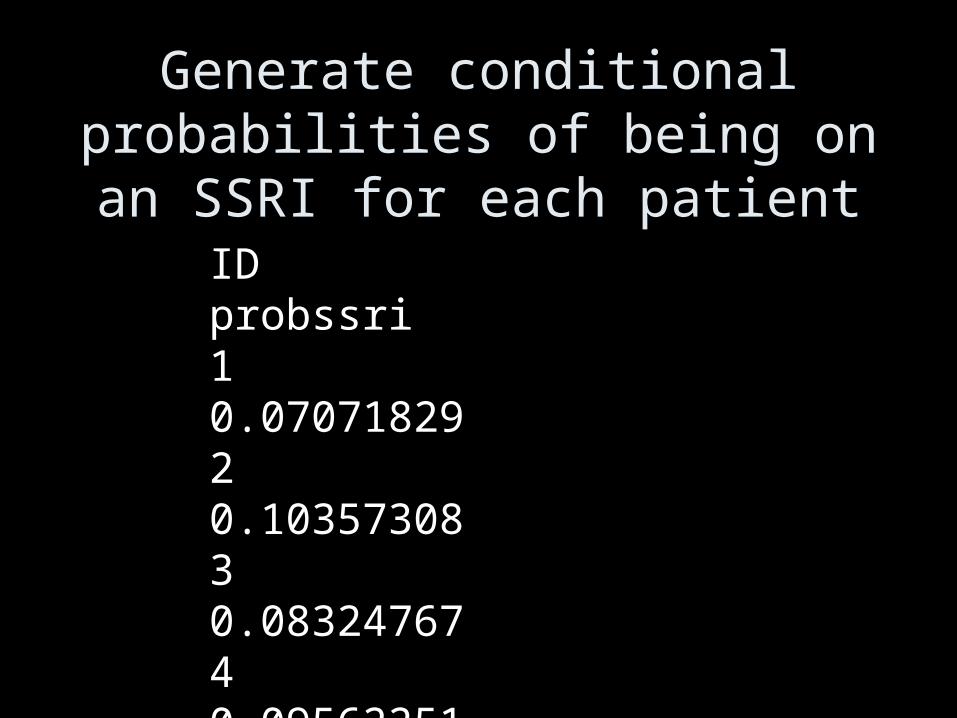
Generate conditional probabilities of being on an SSRI for each
patientID probssri1 0.07071829 2 0.10357308 3 0.083247674 0.09562251 5 0.10424651 6 0.28105882 7 0.09824793

-6 -4 -2 0 2 4
0.0
0.1
0.2
0.3
0.4
lprop
Step 2: Remove non-overlapping cases
SSRI=0SSRI=1
dens
ity
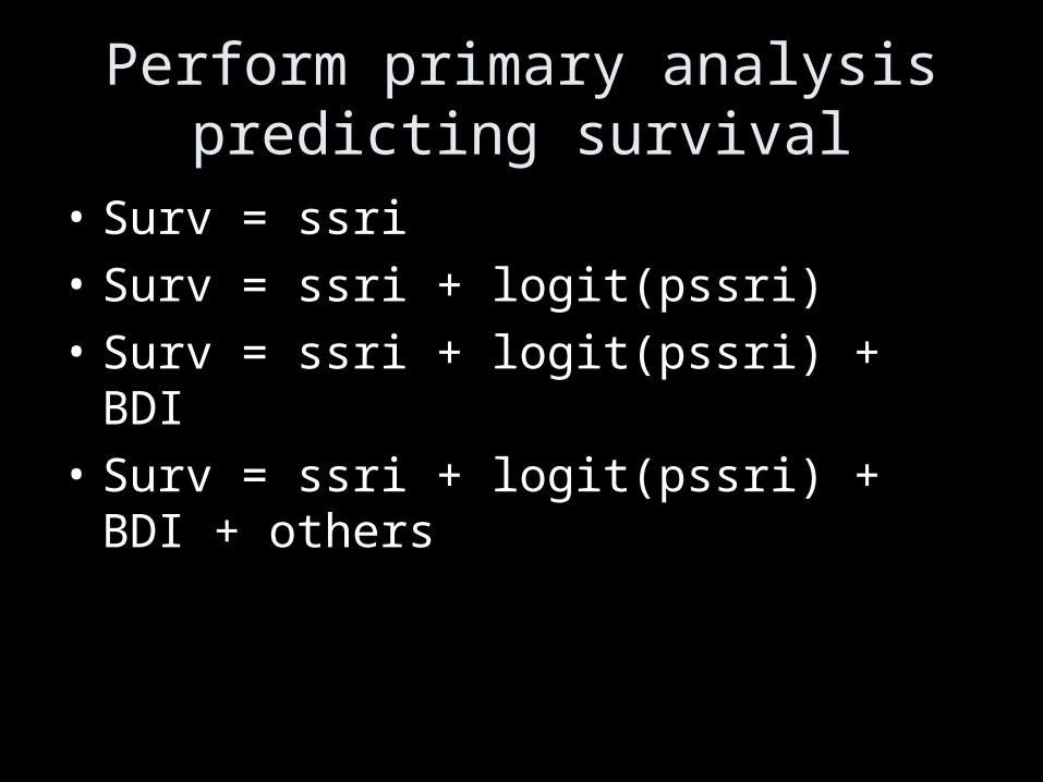
Perform primary analysis predicting survival
• Surv = ssri
• Surv = ssri + logit(pssri)
• Surv = ssri + logit(pssri) + BDI
• Surv = ssri + logit(pssri) + BDI + others

Step 3: Unadjusted estimate
Factor HR Lower 0.95 Upper 0.95 ssri 0.22 0.18 1.05 Hazard Ratio 1.85 1.20 2.86

Step 4: Adjusted for Propensity (linear)
Factor Effect S.E. Lower 0.95 Upper 0.95 ssri 0.61 0.24 0.15 1.08 Hazard Ratio 1.85 NA 1.16 2.95 LOGIT 0.00 0.14 -0.27 0.28 Hazard Ratio 1.00 NA 0.76 1.33
Propensity Score
Pro
b. o
f D
eath
at
3 Y
ears
-4 -3 -2 -1 0 1
0.65
0.70
0.75
0.80
0.85
0.90
Adjusted to: ssri=0
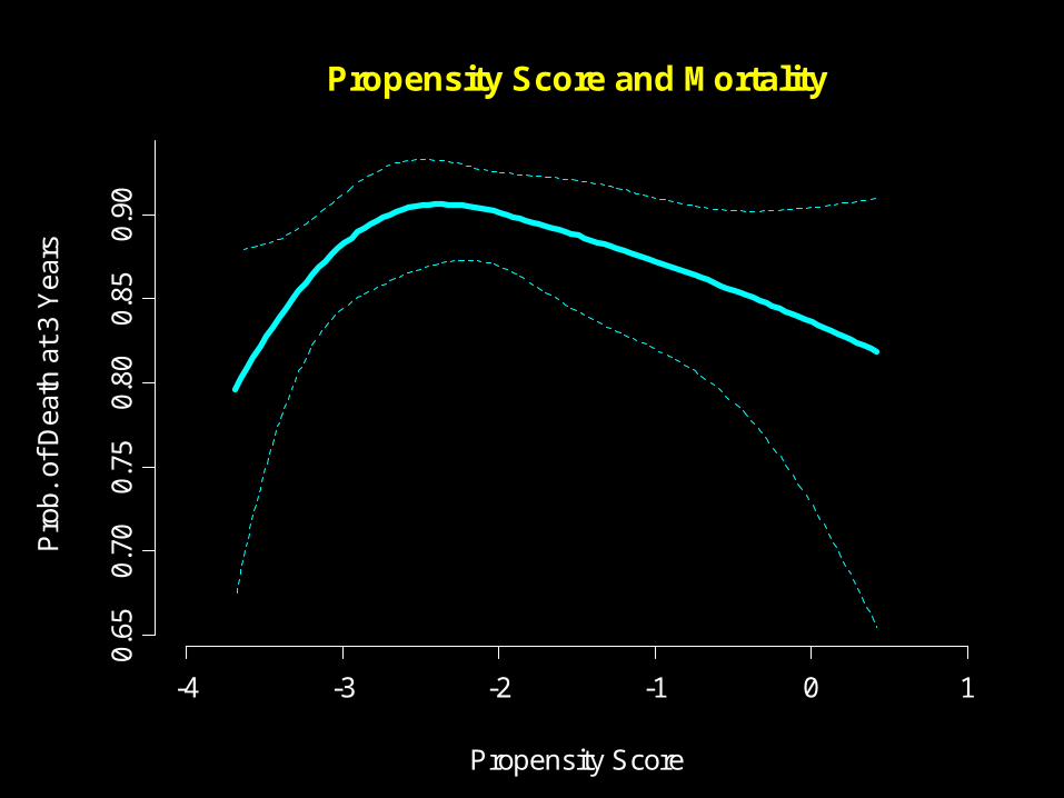
Propensity Score and Mortality

Better Step 4: Adjusted for Propensity (non-linear)
Factor Effect S.E. Lower 0.95 Upper 0.95 ssri 0.55 0.24 0.07 1.03 Hazard Ratio 1.73 NA 1.07 2.79 LOGIT 0.02 0.25 -0.47 0.51 Hazard Ratio 1.02 NA 0.62 1.67

Hazard Ratio
0.40 0.75 1.20 1.60 2.00 2.40 2.80
ssri - 1:0LOGIT - -1.5:-2.9
bdiscore - 10:3age - 70:53lvef - 65:46white - 1:0
risk - 2:1nyh - 1:4/5
0.95
nyh - 2:4/5nyh - 3:4/5
smoke - 1:0smoke - 4:0
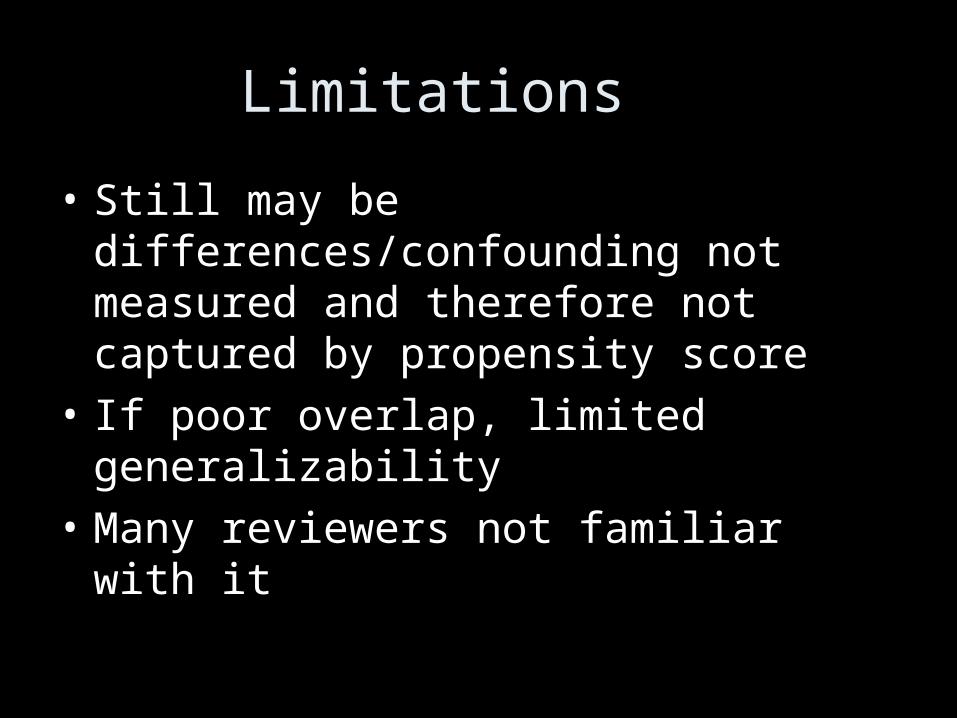
Limitations
• Still may be differences/confounding not measured and therefore not captured by propensity score
• If poor overlap, limited generalizability
• Many reviewers not familiar with it

What to do about heterogeneous slopes?
• We know there is always heterogeneity of slopes, perhaps even important
• Proper test is product interaction term—NOT within subgroups tests (see BMJ series)– Increased error rate– Differential power– Danger of “Accepting the null”– Sparse cells and unstable estimates
• Tension between low power of interaction and high error rate/instability– Especially true in observational data
• I honestly don’t know what to do—any ideas?
If you worry about Type I
• Use pooled test (see, for example, Cohen & Cohen or Harrell)
• If pooled test not significant, stop there
If Type II is a bigger concern
• Report non-significant effects, acknowledging the uncertainty, but conveying need to investigate more
• C.F. HRT data – was there an age X HRT interaction?

Validation• Apparent fit
• Usually too optimistic• Internal
• cross-validation, bootstrap• honest estimate for model
performance• provides an upper limit to what would
be found on external validation• External validation
• replication with new sample, different circumstances

Validation
• Steyerburg, et al. (1999) compared validation methods
• Found that split-half was far too conservative
• Bootstrap was equal or superior to all other techniques

Conclusions• Measure well• Use all the information• Recognize the limitations based on how much
data you actually have• In the confirmatory mode, be as explicit as
possible about the model a priori, test it, and live with it
• By all means, explore data, but recognize— and state frankly --the limits post hoc analysis places on inference

http://myspace.com/monkeynavigatedrobots

Advanced topics and examples
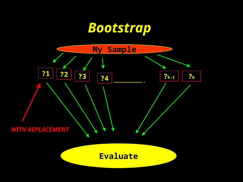
?1………………….
My Sample
Evaluate
Bootstrap
?2 ?3 ?4 ?k-1 ?k
WITH REPLACEMENT

1, 3, 4, 5, 7, 10
7114510
1032221
351427
211727
4414210
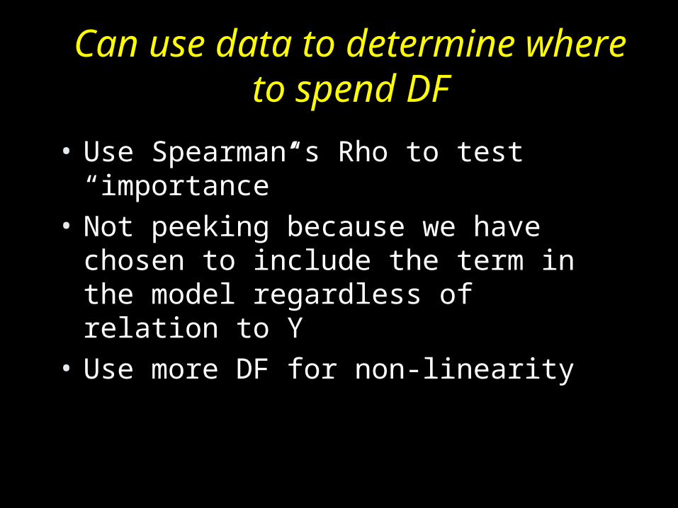
Can use data to determine where to spend DF
• Use Spearman’s Rho to test “importance”
• Not peeking because we have chosen to include the term in the model regardless of relation to Y
• Use more DF for non-linearity

Example-Predict Survival from age, gender, and fare on Titanic:
example using R software

If you have already decided to include them (and promise to keep them in the model) you can peek at predictors in order to see where to add complexity
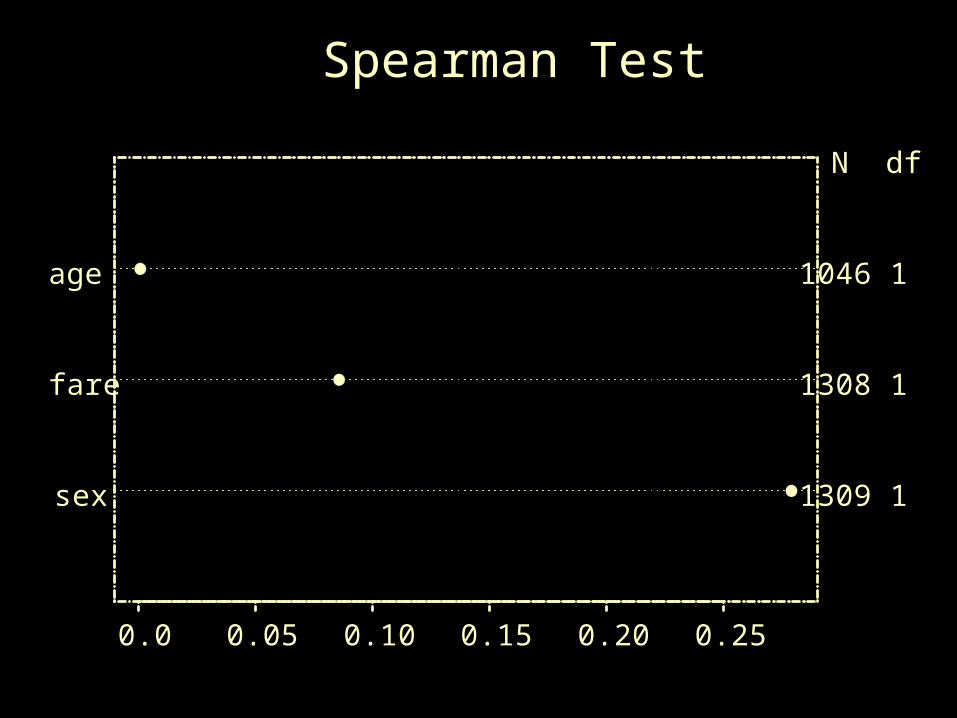
Adjusted rho^2
0.0 0.05 0.10 0.15 0.20 0.25
1046 1
1308 1
1309 1
N df
age
fare
sex
Spearman Test
Non-linearity using splines

0
0.5
1
1.5
2
2.5
0 0 5 10 15 20 25
X
YLinear Spline
(piecewise regression)
Y = a + b1(x<10) + b2(10<x<20) + b3 (x >20)
0
0.5
1
1.5
2
2.5
0 0
X
Y
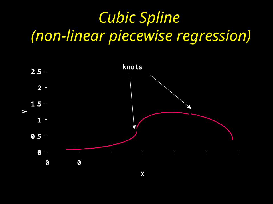
Cubic Spline (non-linear piecewise
regression)
knots
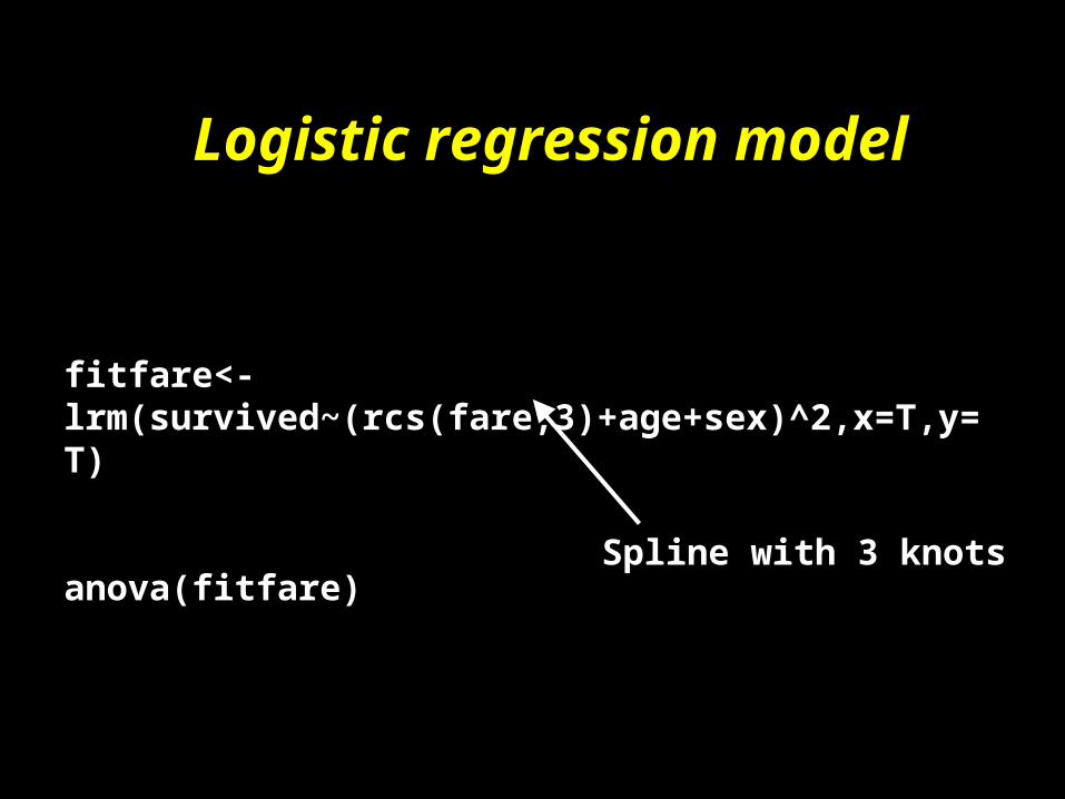
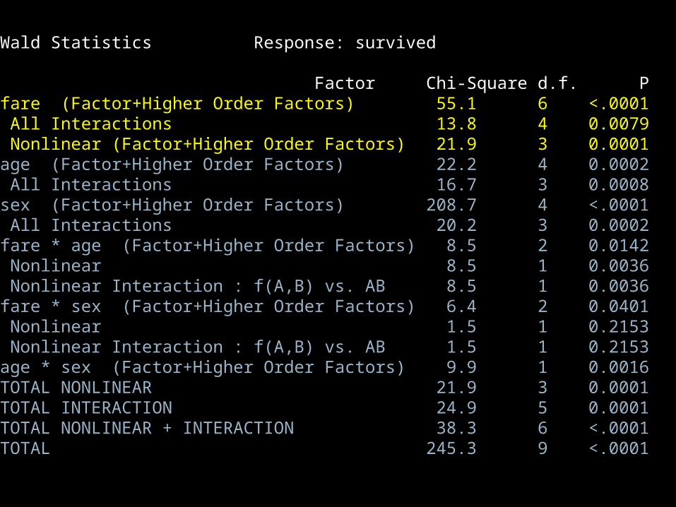
fitfare<-lrm(survived~(rcs(fare,3)+age+sex)^2,x=T,y=T)
anova(fitfare)
Logistic regression model
Spline with 3 knots

Wald Statistics Response: survived
Factor Chi-Square d.f. P fare (Factor+Higher Order Factors) 55.1 6 <.0001 All Interactions 13.8 4 0.0079 Nonlinear (Factor+Higher Order Factors) 21.9 3 0.0001 age (Factor+Higher Order Factors) 22.2 4 0.0002 All Interactions 16.7 3 0.0008 sex (Factor+Higher Order Factors) 208.7 4 <.0001 All Interactions 20.2 3 0.0002 fare * age (Factor+Higher Order Factors) 8.5 2 0.0142 Nonlinear 8.5 1 0.0036 Nonlinear Interaction : f(A,B) vs. AB 8.5 1 0.0036 fare * sex (Factor+Higher Order Factors) 6.4 2 0.0401 Nonlinear 1.5 1 0.2153 Nonlinear Interaction : f(A,B) vs. AB 1.5 1 0.2153 age * sex (Factor+Higher Order Factors) 9.9 1 0.0016 TOTAL NONLINEAR 21.9 3 0.0001 TOTAL INTERACTION 24.9 5 0.0001 TOTAL NONLINEAR + INTERACTION 38.3 6 <.0001 TOTAL 245.3 9 <.0001
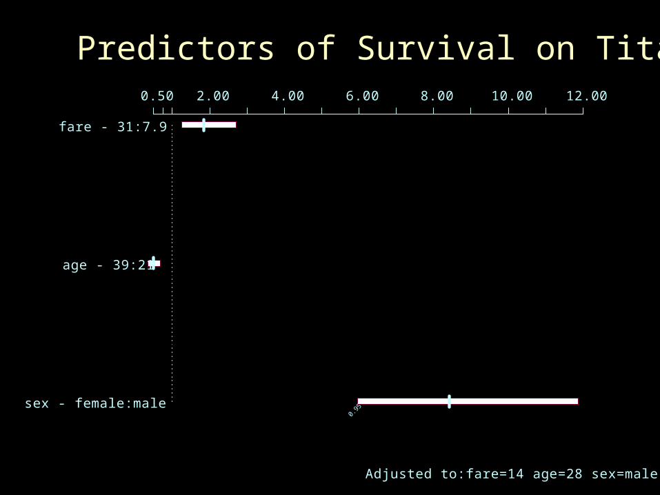
0.50 2.00 4.00 6.00 8.00 10.00 12.00
fare - 31:7.9
age - 39:21
0.95
sex - female:male
Adjusted to:fare=14 age=28 sex=male
Predictors of Survival on Titanic

0
50
100150
200250
Fare10
20
30
40
50
60
age
00.
20.
40.
60.
81
Pro
b. o
f Sur
viva
l
Adjusted to: sex=male
Fare and Age Interaction
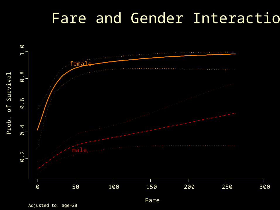
Fare
Pro
b.
of
Su
rviv
al
0 50 100 150 200 250 300
0.2
0.4
0.6
0.8
1.0
female
male
Adjusted to: age=28
Fare and Gender Interaction
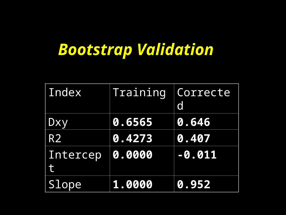
Index Training Corrected
Dxy 0.6565 0.646
R2 0.4273 0.407
Intercept 0.0000 -0.011
Slope 1.0000 0.952
Bootstrap Validation
Summary
• Think about your model• Collect enough data

Summary
• Measure well• Don’t destroy what you’ve
measured

• Pick your variables ahead of time and collect enough data to test the model you want
• Keep all your variables in the model unless extremely unimportant
Summary

• Use more df on important variables, fewer df on “nuisance” variables
• Don’t peek at Y to combine, discard, or transform variables
Summary

• Estimate validity and shrinkage with bootstrap
Summary
• By all means, tinker with the model later, but be aware of the costs of tinkering
• Don’t forget to say you tinkered
• Go collect more data
Summary
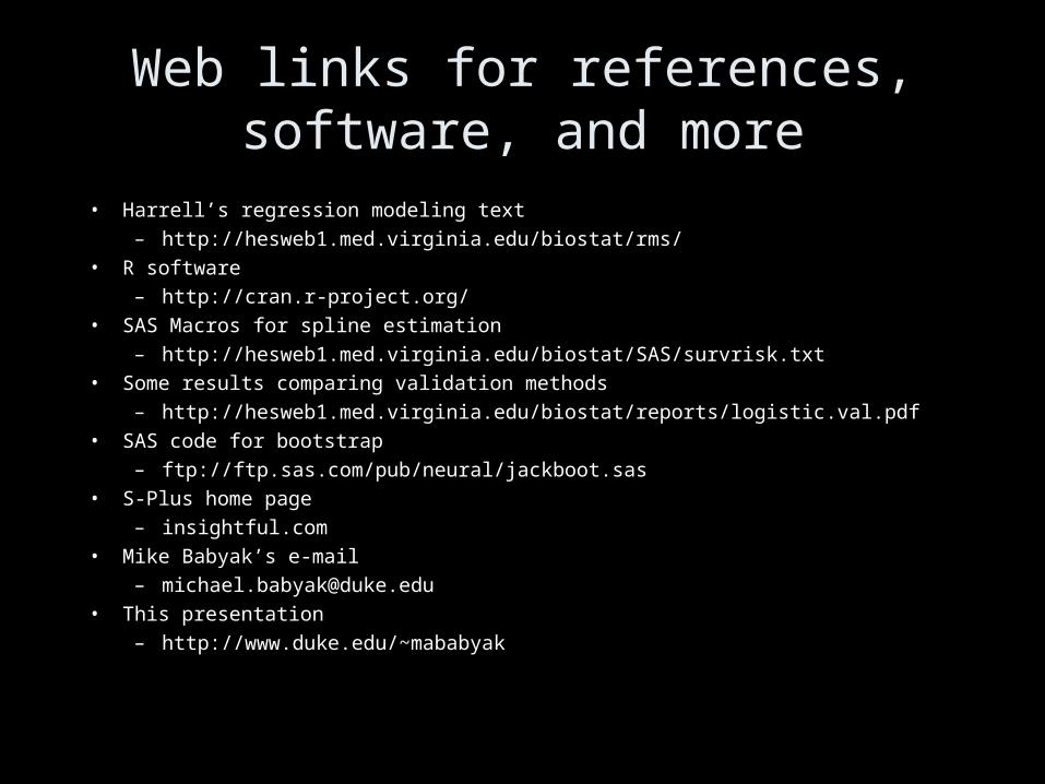
Web links for references, software, and more
• Harrell’s regression modeling text– http://hesweb1.med.virginia.edu/biostat/rms/
• R software– http://cran.r-project.org/
• SAS Macros for spline estimation– http://hesweb1.med.virginia.edu/biostat/SAS/survrisk.txt
• Some results comparing validation methods– http://hesweb1.med.virginia.edu/biostat/reports/logistic.val.pdf
• SAS code for bootstrap– ftp://ftp.sas.com/pub/neural/jackboot.sas
• S-Plus home page– insightful.com
• Mike Babyak’s e-mail – [email protected]
• This presentation– http://www.duke.edu/~mababyak

• www.duke.edu/~mababyak
• michael.babyak @ duke.edu
• symptomresearch.nih.gov/chapter_8/

Observational Data and Clinical Trialshttp://www.epidemiologic.org/2006/11/agreement-of-observational-and.html
http://www.epidemiologic.org/2006/10/resolving-differences-of-studies-of.html
Propensity ScoringRubin Symposium noteshttp://www.symposion.com/nrccs/rubin.htm
Rosenbaum, P.R. and Rubin, D.B. (1984). "Reducing bias in observational studies using sub-classification on the propensity score." Journal of the American Statistical Association, 79, pp. 516-524.
Pearl, J. (2000). Causality: Models, Reasoning, and Inference, Cambridge University Press.
Rosenbaum, P. R., and Rubin, D. B., (1983), "The Central Role of the Propensity Score in Observational Studies for Causal Effects, Biometrica, 70, 41-55. Mediation and ConfoundingMacKinnon DP, Krull JL, Lockwood CM. Equivalence of the mediation, confounding and suppression effect. Prev Sci (2000) 1:173–81

General ModelingHarrell FE Jr. Regression modeling strategies: with applications to linear models, logistic regression and survival analysis. New York: Springer; 2001.
Sample SizeKelley, K. & Maxwell, S. E. (2003). Sample size for Multiple Regression: Obtaining regression coefficients that are accuracy, not simply significant. Psychological Methods, 8, 305–321.
Kelley, K. & Maxwell, S. E. (In press). Power and Accuracy for Omnibus and Targeted Effects: Issues of Sample Size Planning with Applications to Multiple Regression Handbook of Social Research Methods, J. Brannon, P. Alasuutari, and L. Bickman (Eds.). New York, NY: Sage Publications.
Green SB. How many subjects does it take to do a regression analysis? Multivar Behav Res 1991; 26: 499–510.
Peduzzi PN, Concato J, Holford TR, Feinstein AR. The importance of events per independent variable in multivariable analysis, II: accuracy and precision of regression estimates. J Clin Epidemiol 1995; 48: 1503–10
Peduzzi PN, Concato J, Kemper E, Holford TR, Feinstein AR. A simulation study of the number of events per variable in logistic regression analysis. J Clin Epidemiol 1996; 49: 1373–9.

Dichotomization
Cohen, J. (1983) The cost of dichotomization. Applied Psychological Measurement, 7, 249-253.
MacCallum R.C., Zhang, S., Preacher, K.J., & Rucker, D.D. (2002). On the practice of dichotomization of quantitative variables. Psychological Methods, 7(1), 19-40.
Maxwell, SE, & Delaney, HD (1993). Bivariate median splits and spurious statistical significance. Psychological Bulletin, 113, 181-190
Royston, P., Altman, D. G., & Sauerbrei, W. (2006) Dichotomizing continuous predictors in multiple regression: a bad idea. Statistics in Medicine, 25,127-141.
http://biostat.mc.vanderbilt.edu/twiki/bin/view/Main/CatContinuous
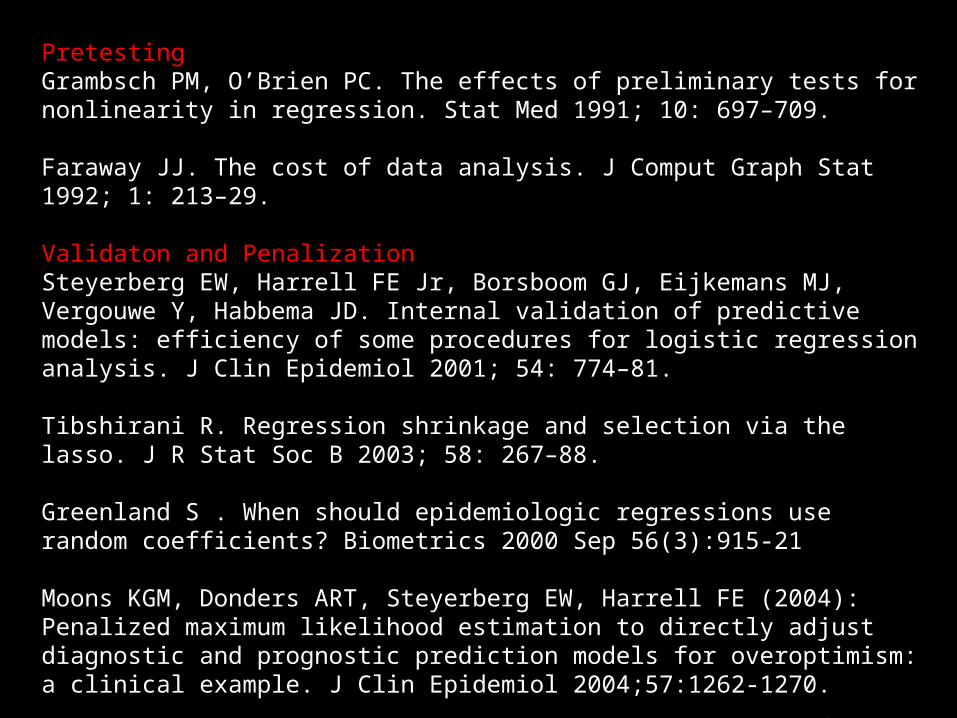
PretestingGrambsch PM, O’Brien PC. The effects of preliminary tests for nonlinearity in regression. Stat Med 1991; 10: 697–709.
Faraway JJ. The cost of data analysis. J Comput Graph Stat 1992; 1: 213–29.
Validaton and PenalizationSteyerberg EW, Harrell FE Jr, Borsboom GJ, Eijkemans MJ, Vergouwe Y, Habbema JD. Internal validation of predictive models: efficiency of some procedures for logistic regression analysis. J Clin Epidemiol 2001; 54: 774–81.
Tibshirani R. Regression shrinkage and selection via the lasso. J R Stat Soc B 2003; 58: 267–88.
Greenland S . When should epidemiologic regressions use random coefficients? Biometrics 2000 Sep 56(3):915-21
Moons KGM, Donders ART, Steyerberg EW, Harrell FE (2004): Penalized maximum likelihood estimation to directly adjust diagnostic and prognostic prediction models for overoptimism: a clinical example. J Clin Epidemiol 2004;57:1262-1270.
Steyerberg EW, Eijkemans MJ, Habbema JD. Application of shrinkage techniques in logistic regression analysis: a case study. Stat Neerl 2001; 55:76-88.
Variable SelectionThompson B. Stepwise regression and stepwise discriminant analysis need not apply here: a guidelines editorial. Ed Psychol Meas 1995; 55: 525–34.
Altman DG, Andersen PK. Bootstrap investigation of the stability of a Cox regression model. Stat Med 2003; 8: 771–83.
Derksen S, Keselman HJ. Backward, forward and stepwise automated subset selection algorithms: frequency of obtaining authentic and noise variables. Br J Math Stat Psychol 1992; 45: 265–82.
Steyerberg EW, Harrell FE, Habbema JD. Prognostic modeling with logistic regression analysis: in search of a sensible strategy in small data sets. Med Decis Making 2001; 21: 45–56.
Cohen J. Things I have learned (so far). Am Psychol 1990; 45: 1304–12.
Roecker EB. Prediction error and its estimation for subset-selected models Technometrics 1991; 33: 459–68.