modeling without categorical variables: a mixed-integer · pdf file · 2009-03-30on...
TRANSCRIPT
ARGONNE NATIONAL LABORATORY
9700 South Cass Avenue
Argonne, Illinois 60439
Modeling without Categorical Variables: A Mixed-Integer NonlinearProgram for the Optimization of Thermal Insulation Systems 1
Kumar Abhishek, Sven Leyffer, and Jeffrey T. Linderoth
Mathematics and Computer Science Division
Preprint ANL/MCS-P1434-0607
June 21, 2007
1This work was supported in part by the Mathematical, Information, and Computational Sciences Division subprogram of the
Office of Advanced Scientific Computing Research, Office of Science,U.S. Department of Energy, under Contract DE-AC02-
06CH11357. This work was also supported by the U.S. Department of Energy through the grant DE-FG02-05ER25694.

Contents
1 Introduction 1
2 Load-Bearing Thermal Insulation Design 2
2.1 Model Parameters and Data . . . . . . . . . . . . . . . . . . . . . . . . . . . . . .. . . . . 2
2.2 Model Variables . . . . . . . . . . . . . . . . . . . . . . . . . . . . . . . . . . . . .. . . . 4
2.3 Mixed-Variable Optimization Model . . . . . . . . . . . . . . . . . . . . . . . . . . .. . . 5
2.4 Challenges of the MVP Model . . . . . . . . . . . . . . . . . . . . . . . . . . . . .. . . . 6
3 Modeling Categorical Variables with Binary Variables 8
4 A MINLP Model for Thermal Insulation Design 12
4.1 Avoiding Bilevel Optimization Problems . . . . . . . . . . . . . . . . . . . . . . . . . .. . 12
4.2 Evaluation of Integrals . . . . . . . . . . . . . . . . . . . . . . . . . . . . . . . . .. . . . 13
4.3 Modeling a Discontinuous Function with Binary Variables . . . . . . . . . . . .. . . . . . 16
4.4 A Piecewise Smooth MINLP Model . . . . . . . . . . . . . . . . . . . . . . . . . . .. . . 17
5 A Smooth MINLP Model with Discretized Temperature 18
6 Solution Methodology and Computational Results 21
7 Conclusions 29
Modeling without Categorical Variables: A Mixed-Integer Nonlinear
Program for the Optimization of Thermal Insulation Systems∗
KUMAR ABHISHEK† , SVEN LEYFFER‡ , AND JEFFREYT. L INDEROTH§
June 21, 2007
Abstract
Optimal design applications are often modeled by using categorical variables to express discrete design
decisions, such as material types. A disadvantage of using categorical variables is the lack of continu-
ous relaxations, which precludes the use of modern integer programming techniques. We show how to
express categorical variables with standard integer modeling techniques, and we illustrate this approach
on a load-bearing thermal insulation system. The system consists of a number of insulators of different
materials and intercepts that minimize the heat flow from a hot surface to a cold surface. Our new model
allows us to employ black-box modeling languages and solvers and illustrates the interplay between in-
teger and nonlinear modeling techniques. We present numerical experience that illustrates the advantage
of the standard integer model.
Keywords: Mixed integer nonlinear programming, modeling with binaryvariables, thermal insulation
systems, categorical variables.
AMS-MSC2000: 90C11, 90C30, 90C90
1 Introduction
Recently, researchers have expressed interest in mixed-variable optimization problems (MVPs). Problems
of this class involvecategorical variables, which are constrained to take values from a finite set of non-
numerical values. MVPs have been used to design load-bearing thermal insulation systems, where the cat-
egorical variables model the type of material chosen for the insulators (Kokkolaras et al., 2001; Abramson,
∗Preprint ANL/MCS-P1434-0607.†Department of Industrial and Systems Engineering, Lehigh University, Bethlehem, PA 18015,[email protected].‡Mathematics and Computer Science Division, Argonne National Laboratory, Argonne, IL 60439,[email protected].§Department of Industrial and Systems Engineering, Lehigh University, Bethlehem, PA 18015,[email protected].
1
2 Kumar Abhishek, Sven Leyffer, and Jeffrey T. Linderoth
2004). Categorical variables are a convenient way to move from a simulation tool that requires input such
as material properties to an optimization tool. On the other hand, the presence of categorical variables pre-
cludes the use of modern integer optimization techniques, because continuous relaxations of the categorical
decisions are not readily available.
We show how categorical variables can be replaced by standard integermodeling techniques. We illus-
trate our approach on an example of thermal insulation systems and emphasizethe interaction of integer and
nonlinear modeling techniques. Our approach provides a blueprint for reformulating other design problems
that involve categorical variables, for example the design of nanomaterials(Zhao et al., 2005), and in op-
timal sensor placement (Beal et al., 2006). We believe that the conclusionsof this paper also are relevant
to application scientists who develop simulation tools. In our view it is important to include optimization
considerations in simulation tools from the start.
This paper is organized as follows. We start by reviewing the categoricalvariable formulation of a
thermal insulation system. Next, we introduce the integer and nonlinear modeling techniques that allow us
to reformulate this model as a standard mixed integer nonlinear programming (MINLP) model. We obtain
three models with varying degree of smoothness and comment on the relative merits of these formulations.
Numerical experiments illustrating the benefit of our new approach are presented.
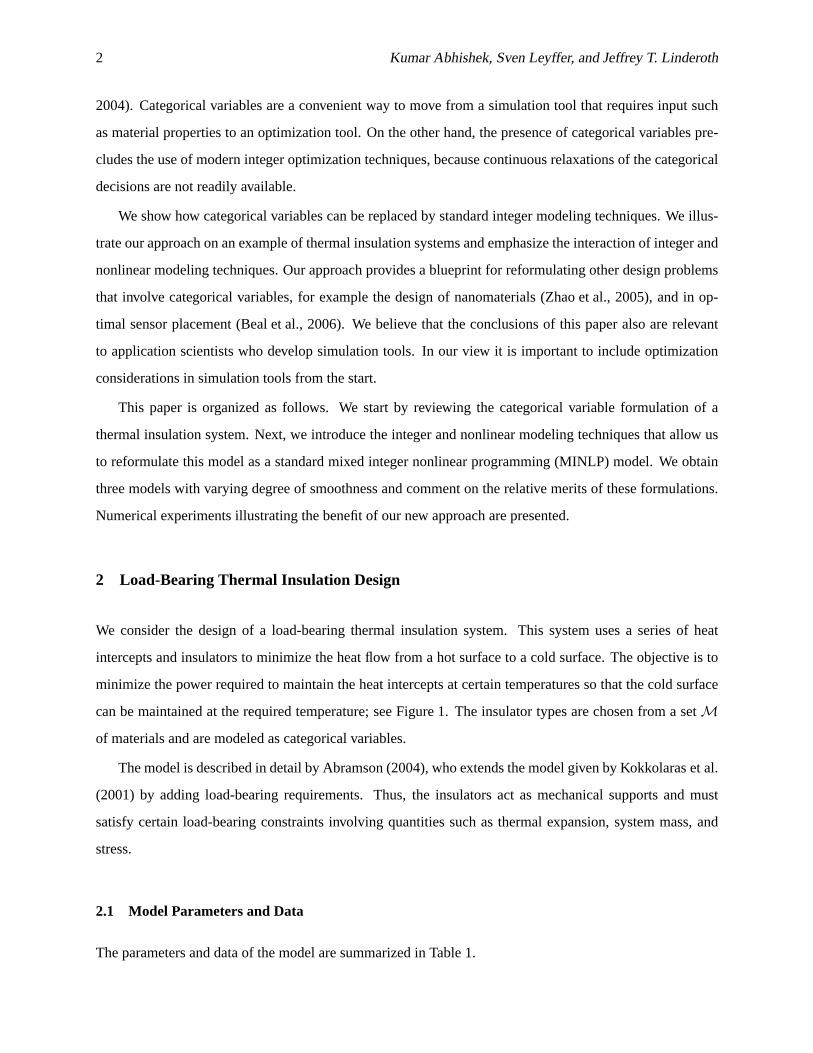
2 Load-Bearing Thermal Insulation Design
We consider the design of a load-bearing thermal insulation system. This system uses a series of heat
intercepts and insulators to minimize the heat flow from a hot surface to a cold surface. The objective is to
minimize the power required to maintain the heat intercepts at certain temperaturesso that the cold surface
can be maintained at the required temperature; see Figure 1. The insulator types are chosen from a setM
of materials and are modeled as categorical variables.
The model is described in detail by Abramson (2004), who extends the model given by Kokkolaras et al.
(2001) by adding load-bearing requirements. Thus, the insulators act as mechanical supports and must
satisfy certain load-bearing constraints involving quantities such as thermalexpansion, system mass, and
stress.
2.1 Model Parameters and Data
The parameters and data of the model are summarized in Table 1.

Modeling without Categorical Variables: A MINLP Model for Thermal Insulation Systems 3
� � � � � � � � � � � � � � � � � �� � � � � � � � � � � � � � � � � �� � � � � � � � � � � � � � � � � �� � � � � � � � � � � � � � � � � �
� �� �� �� �
� �� �� �� �
� � � � � � � � � � � � � � � � � �� � � � � � � � � � � � � � � � � �� � � � � � � � � � � � � � � � � �
� � � � � � � � � � � � � � � � � �� � � � � � � � � � � � � � � � � �� � � � � � � � � � � � � � � � � �
� � � �� � � �� � � �
� � �� � �� � �
� � �� � �� � �
� � �� � �� � �� � �� � �� � �
tn+1 = TH
ti+1
ti
ti−1
t0 = TC
xi+1L
xi
Figure 1: Illustration of the thermal insulation system.
Table 1: Model Parameters and Data
Parameter Description Value in Case Study Instance
C(ti) thermodynamic cycle efficiency of intercepti, see (2.1)
e(t, m) thermal expansion of insulatorm ∈ M at temperaturet
F system load 250 kN
k(t, m) thermal conductivity of insulatorm ∈ M at temperaturet
L system length 10 cm
M maximum system mass 10 kg
M set of insulator materials see Table 2
N maximum number of intercepts 10
TC cold surface temperature 4.2K
TH hot surface temperature 300K
δ maximum thermal expansion 5%
ρ(m) density of insulatorm ∈ M see Table 2
σ(t, m) tensile yield strength of insulatorm ∈ M at temperaturet
4 Kumar Abhishek, Sven Leyffer, and Jeffrey T. Linderoth
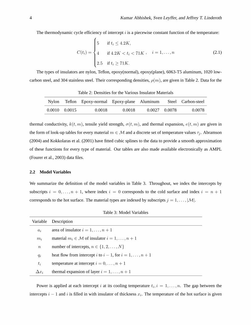
The thermodynamic cycle efficiency of intercepti is a piecewise constant function of the temperature:
C(ti) =
5 if ti ≤ 4.2K,
4 if 4.2K < ti < 71K
2.5 if ti ≥ 71K.
, i = 1, . . . , n (2.1)
The types of insulators are nylon, Teflon, epoxy(normal), epoxy(plane), 6063-T5 aluminum, 1020 low-
carbon steel, and 304 stainless steel. Their corresponding densities,ρ(m), are given in Table 2. Data for the
Table 2: Densities for the Various Insulator Materials
Nylon Teflon Epoxy-normal Epoxy-plane Aluminum Steel Carbon-steel
0.0010 0.0015 0.0018 0.0018 0.0027 0.0078 0.0078
thermal conductivity,k(t, m), tensile yield strength,σ(t, m), and thermal expansion,e(t, m) are given in
the form of look-up tables for every materialm ∈ M and a discrete set of temperature valuesτj . Abramson
(2004) and Kokkolaras et al. (2001) have fitted cubic splines to the data toprovide a smooth approximation
of these functions for every type of material. Our tables are also made available electronically as AMPL
(Fourer et al., 2003) data files.
2.2 Model Variables
We summarize the definition of the model variables in Table 3. Throughout, we index the intercepts by
subscriptsi = 0, . . . , n + 1, where indexi = 0 corresponds to the cold surface and indexi = n + 1
corresponds to the hot surface. The material types are indexed by subscriptsj = 1, . . . , |M|.
Table 3: Model Variables
Variable Description
ai area of insulatori = 1, . . . , n + 1
mi materialmi ∈ M of insulatori = 1, . . . , n + 1
n number of intercepts,n ∈ {1, 2, . . . , N}
qi heat flow from intercepti to i − 1, for i = 1, . . . , n + 1
ti temperature at intercepti = 0, . . . , n + 1
∆xi thermal expansion of layeri = 1, . . . , n + 1
Power is applied at each intercepti at its cooling temperatureti, i = 1, . . . , n. The gap between the
interceptsi − 1 andi is filled in with insulator of thicknessxi. The temperature of the hot surface is given
Modeling without Categorical Variables: A MINLP Model for Thermal Insulation Systems 5
by tn+1 = TH and that of the cold surface byt0 = TC . The insulators used in the system may have
different cross-sectional areasai. The design of the system involves choosing the number of interceptsn,
their cooling temperaturesti, the insulator typesmi, their thicknessxi and the cross-sectional areasai. We
include the thermal expansion,∆xi/xi for convenience but note that it is later eliminated from the model.
The presence of categorical variables such as insulator typesmi and the number of insulatorsn make the
model into a mixed-variable program.
2.3 Mixed-Variable Optimization Model
We can now state the complete mixed-variable optimization model.
minimizen
∑
i=1
C(ti)
(
TH
ti− 1
)
· (qi+1 − qi) (2.2)
subject to qi =ai
xi
∫ ti
ti−1
k(t, mi)dt, i = 1, . . . , n + 1 (2.3)
n∑
i=1
ρ(mi)aixi ≤ M (2.4)
F
ai
≤ σi = min{σ(t, mi) : ti−1 ≤ t ≤ ti}, i = 1, . . . , n + 1 (2.5)
n∑
i=1
(
∆xi
xi
)
(xi
L
)
≤δ
100(2.6)
∆xi
xi
=
∫ titi−1
e(t, mi)k(t, mi)dt∫ titi−1
k(t, mi)dt, i = 1, . . . , n (2.7)
n∑
i=1
xi = L (2.8)
ti−1 ≤ ti ≤ ti+1, i = 1, . . . , n (2.9)
t0 = TC and tn+1 = TH (2.10)
xi ≥ 0, ai ≥ 0, i = 1, . . . , n + 1 (2.11)
The model contains five classes of nonlinear constraints. Equation (2.3) defines the heat flow from
intercepti to i − 1, which is governed by Fourier’s law. Equation (2.4) is the mass constraintof the system.
The stress of the system must not exceed the specified loadF , which is modeled by Equation (2.5). The
thermal expansion constraint is modeled by Equation (2.6), with the thermal contraction∆xi
xidefined by the
constraint (2.7). In addition, the model contains some linear constraints: (2.8) constrains the thickness of
the design, (2.9) orders the temperatures, and (2.10) fixes the temperatures at the cold and hot surface. We
note that the latter two constraints imply thatTC ≤ ti ≤ TH for i = 0, . . . , N + 1.
6 Kumar Abhishek, Sven Leyffer, and Jeffrey T. Linderoth
Abramson (2004) uses a different objective function in hismatlab implementation, namely,
f2 :=
n+1∑
i=1
qi
(
C(ti−1)(TH
ti−1− 1) − C(ti)(
TH
ti− 1)
)
. (2.12)
We use this objective function from now on for the purpose of modeling andfor comparing our results with
the work of Abramson.
The integrals in (2.3) and (2.7) are approximated by Simpson’s rule, wherethe material specific functions
e(t, mi) andk(t, mi) are derived from cubic spline interpolation of tabulated data.
Solving the thermal insulation problem involves evaluating a nonlinear objective function and nonlinear
constraints over a variable space that includes categorical variables. The model is solved by using a pattern-
search algorithm (Audet and Dennis, 2004, 2000; Abramson et al., 2004). The computational burden of
pattern-search techniques grows with the number of variables, and this fact motivates the removal of as
many defined variables as possible. For example, the fixed variablest0 and tn+1 are removed. We can
also remove the thermal expansion variables∆xi
xiby substituting (2.7) into (2.6). In addition, it is argued in
(Abramson, 2004) that the stress constraint must be binding at a solution,thereby implying thatai = Fσi
and
allowing us to remove the variablesai.
2.4 Challenges of the MVP Model
The MVP model (2.2)–(2.10) introduces a number of difficulties that appear to make it impossible to employ
standard MINLP techniques to solve the problem:
1. The model contains a number of categorical variables that do not allow continuous relaxations. For
example, it is not clear how to relax the condition that the materials be chosen fromM. Worse, the
variablen appears as the upper limit in the summation, which makes constraints such as (2.8), (2.4),
(2.6), and the objective function ((2.2) or (2.12)) discontinuous. Moreover, by changingn, we also
change the number of variablesti and so forth that appear in the model. In this sense, everyn defines
a different model.
2. There exists no analytic closed-form expression for the integrals in (2.3) and (2.7). Instead, the in-
tegrals are evaluated by using Simpson’s rule. Thus, derivatives are difficult to compute, and hence
derivative-free optimization techniques are used.
3. Constraint (2.5) contains a minimization for which no closed-form expression exists. The presence of
this constraint results in a bilevel optimization problem that is considerably harder to solve. We note
Modeling without Categorical Variables: A MINLP Model for Thermal Insulation Systems 7
that this constraint can be written equivalently as an infinite set constraint, by requiring that
F
ai
≤ σi(t, mi), ∀t ∈ [ti−1, ti], ∀i = 1, . . . , n + 1.
4. The objective function is discontinuous because of the presence of the thermodynamic cycle efficiency
coefficients,C(ti); see (2.1). This discontinuity can cause derivative-based NLP solvers to fail.
Each of these points is a potential death-blow for standard optimization techniques. Worse, even though
pattern-search techniques can be applied, the discontinuities imply that it is almost impossible to verify the
optimality of a solution returned by the pattern-search method.
Another drawback of pattern-search techniques is the fact that the quality of the solution depends on
the definition of the neighborhood for the search. It is not hard to construct examples where the MVP
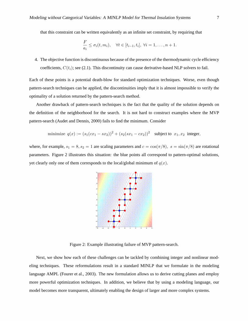
pattern-search (Audet and Dennis, 2000) fails to find the minimum. Consider
minimize q(x) := (s1(cx1 − sx2))2 + (s2(sx1 − cx2))
2 subject tox1, x2 integer,
where, for example,s1 = 8, s2 = 1 are scaling parameters andc = cos(π/8), s = sin(π/8) are rotational
parameters. Figure 2 illustrates this situation: the blue points all correspond topattern-optimal solutions,
yet clearly only one of them corresponds to the local/global minimum ofq(x).
−5 −4 −3 −2 −1 0 1 2 3 4 5−5
−4
−3
−2
−1
0
1
2
3
4
5
Figure 2: Example illustrating failure of MVP pattern-search.
Next, we show how each of these challenges can be tackled by combining integer and nonlinear mod-
eling techniques. These reformulations result in a standard MINLP that weformulate in the modeling
language AMPL (Fourer et al., 2003). The new formulation allows us to derive cutting planes and employ
more powerful optimization techniques. In addition, we believe that by using amodeling language, our
model becomes more transparent, ultimately enabling the design of larger and more complex systems.
8 Kumar Abhishek, Sven Leyffer, and Jeffrey T. Linderoth
3 Modeling Categorical Variables with Binary Variables
We start by showing that the categorical variables can be replaced by integer variables, and we develop a
derivative-free model of thermal insulation that allows relaxations to be computed. We use binary indicator
variablesyi to remove the variablen (the number of intercepts) from the summation bound in (2.4) and
(2.6) and to eliminate the dependence of the number of decision variables on the decision variablen; we
use binary decision variablesyi to denote the existence of layeri. This is a natural reformulation and not
necessarily inefficient in practice, since the maximum number of interceptsN is typically small. For the
specific instance we solve in Section 6,N = 20. This reformulation is made by introducing the following
inequality system:
N+1∑
i=1
yi = n + 1 (3.13)
yi+1 ≤ yi, i = 1, . . . , N (3.14)
xi ≤ Lyi i = 1, . . . , N + 1 (3.15)
yi ∈ {0, 1}, i = 1, . . . , N + 1.
The inequalities (3.14) order the intercepts and ensure that only consecutive intercepts in this ordering can
exist. The variable upper bound inequalities (3.15) ensure that there is a positive thickness to the layer only
if the layer is chosen to exist. The inequalities (3.15) can be replaced by the much stronger set of inequalities
N+1∑
j=i
xj ≤ Lyi i = 1, . . . , N + 1. (3.16)
In fact, Theorem 3.1 establishes that the inequalities (3.16) are facets of the convex hull of the inequality
system of the reformulation.
Theorem 3.1. Let
P = conv(
{(x, y) ∈ RN+1+ × B
N+1+ | yi+1 ≤ yi i = 1, . . . , N, xi ≤ Lyi i = 1, . . . , N + 1}
)
.
ThenN+1∑
j=i
xj ≤ Lyi
defines a facet ofP for eachi = 1, 2, . . . , N + 1.
Proof. Assume that for eachi = 1, . . . , N + 1 there is an inequalityπix + µiy ≤ πi0 that is valid forP and
satisfies
Fidef= {(x, y) ∈ P |
N+1∑
j=i
xj = Lyi} ⊆ {(x, y) ∈ P | πix + µiy = πi0}
def= Fi.
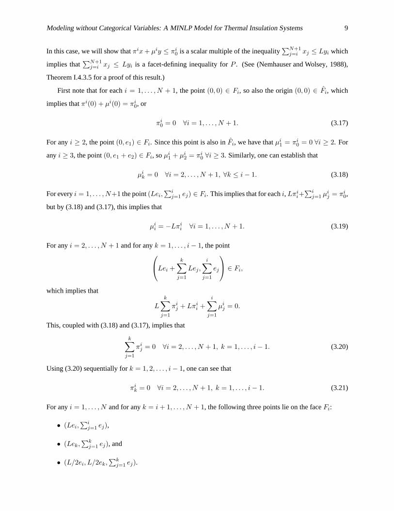
Modeling without Categorical Variables: A MINLP Model for Thermal Insulation Systems 9
In this case, we will show thatπix + µiy ≤ πi0 is a scalar multiple of the inequality
∑N+1j=i xj ≤ Lyi which
implies that∑N+1
j=i xj ≤ Lyi is a facet-defining inequality forP . (See (Nemhauser and Wolsey, 1988),
Theorem I.4.3.5 for a proof of this result.)
First note that for eachi = 1, . . . , N + 1, the point(0, 0) ∈ Fi, so also the origin(0, 0) ∈ Fi, which
implies thatπi(0) + µi(0) = πi0, or
πi0 = 0 ∀i = 1, . . . , N + 1. (3.17)
For anyi ≥ 2, the point(0, e1) ∈ Fi. Since this point is also inFi, we have thatµi1 = πi
0 = 0 ∀i ≥ 2. For
anyi ≥ 3, the point(0, e1 + e2) ∈ Fi, soµi1 + µi
2 = πi0 ∀i ≥ 3. Similarly, one can establish that
µik = 0 ∀i = 2, . . . , N + 1, ∀k ≤ i − 1. (3.18)
For everyi = 1, . . . , N+1 the point(Lei,∑i
j=1 ej) ∈ Fi. This implies that for eachi, Lπii+
∑ij=1 µi
j = πi0,
but by (3.18) and (3.17), this implies that
µii = −Lπi
i ∀i = 1, . . . , N + 1. (3.19)
For anyi = 2, . . . , N + 1 and for anyk = 1, . . . , i − 1, the point
Lei +k
∑
j=1
Lej ,i
∑
j=1
ej
∈ Fi,
which implies that
L
k∑
j=1
πij + Lπi
i +
i∑
j=1
µij = 0.
This, coupled with (3.18) and (3.17), implies that
k∑
j=1
πij = 0 ∀i = 2, . . . , N + 1, k = 1, . . . , i − 1. (3.20)
Using (3.20) sequentially fork = 1, 2, . . . , i − 1, one can see that
πik = 0 ∀i = 2, . . . , N + 1, k = 1, . . . , i − 1. (3.21)
For anyi = 1, . . . , N and for anyk = i + 1, . . . , N + 1, the following three points lie on the faceFi:
• (Lei,∑i
j=1 ej),
• (Lek,∑k
j=1 ej), and
• (L/2ei, L/2ek,∑k
j=1 ej).
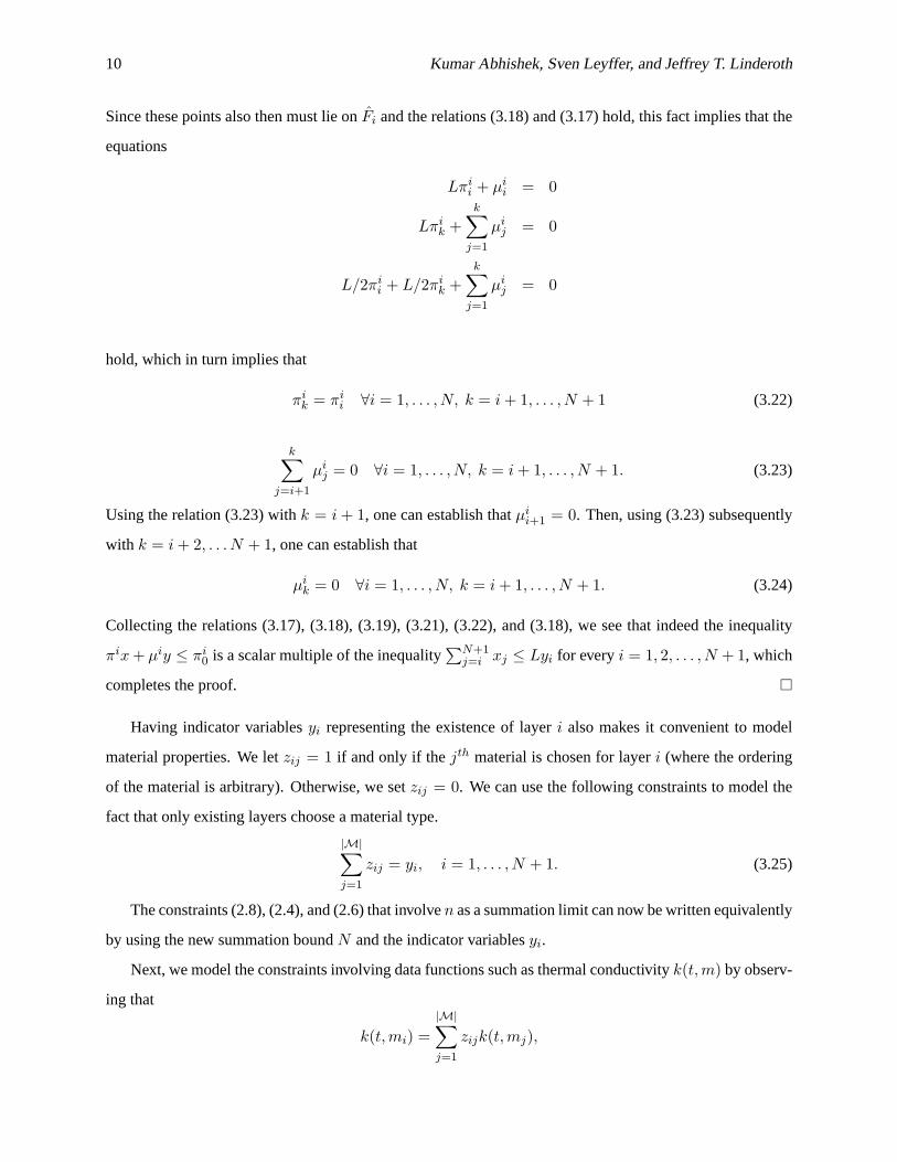
10 Kumar Abhishek, Sven Leyffer, and Jeffrey T. Linderoth
Since these points also then must lie onFi and the relations (3.18) and (3.17) hold, this fact implies that the
equations
Lπii + µi
i = 0
Lπik +
k∑
j=1
µij = 0
L/2πii + L/2πi
k +k
∑
j=1
µij = 0
hold, which in turn implies that
πik = πi
i ∀i = 1, . . . , N, k = i + 1, . . . , N + 1 (3.22)
k∑
j=i+1
µij = 0 ∀i = 1, . . . , N, k = i + 1, . . . , N + 1. (3.23)
Using the relation (3.23) withk = i + 1, one can establish thatµii+1 = 0. Then, using (3.23) subsequently
with k = i + 2, . . . N + 1, one can establish that
µik = 0 ∀i = 1, . . . , N, k = i + 1, . . . , N + 1. (3.24)
Collecting the relations (3.17), (3.18), (3.19), (3.21), (3.22), and (3.18), we see that indeed the inequality
πix + µiy ≤ πi0 is a scalar multiple of the inequality
∑N+1j=i xj ≤ Lyi for everyi = 1, 2, . . . , N + 1, which
completes the proof.
Having indicator variablesyi representing the existence of layeri also makes it convenient to model
material properties. We letzij = 1 if and only if thejth material is chosen for layeri (where the ordering
of the material is arbitrary). Otherwise, we setzij = 0. We can use the following constraints to model the
fact that only existing layers choose a material type.
|M|∑
j=1
zij = yi, i = 1, . . . , N + 1. (3.25)
The constraints (2.8), (2.4), and (2.6) that involven as a summation limit can now be written equivalently
by using the new summation boundN and the indicator variablesyi.
Next, we model the constraints involving data functions such as thermal conductivity k(t, m) by observ-
ing that
k(t, mi) =
|M|∑
j=1
zijk(t, mj),
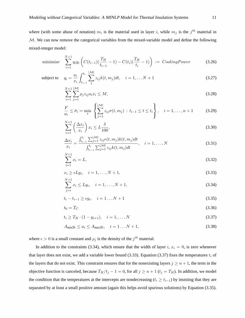
Modeling without Categorical Variables: A MINLP Model for Thermal Insulation Systems 11
where (with some abuse of notation)mi is the material used in layeri, while mj is the jth material in
M. We can now remove the categorical variables from the mixed-variable model and define the following
mixed-integer model:
minimizeN+1∑
i=1
qiyi
(
C(ti−1)(TH
ti−1− 1) − C(ti)(
TH
ti− 1)
)
:= CoolingPower (3.26)
subject to qi =ai
xi
∫ ti
ti−1
|M|∑
1
zijk(t, mj)dt, i = 1, . . . N + 1 (3.27)
N+1∑
i=1
|M|∑
j=1
ρjzijaixi ≤ M, (3.28)
F
ai
≤ σi = mint
|M|∑
j=1
zijσ(t, mj) : ti−1 ≤ t ≤ ti
, i = 1, . . . , n + 1 (3.29)
N+1∑
i=1
(
∆xi
xi
)
xi ≤ Lδ
100, (3.30)
∆xi
xi
=
∫ titi−1
∑|M|j=1 zije(t, mj)k(t, mj)dt
∫ titi−1
∑|M|j=1 zijk(t, mj)dt
, i = 1, . . . , N (3.31)
N+1∑
i=1
xi = L, (3.32)
xi ≥ εLyi, i = 1, . . . , N + 1, (3.33)
N+1∑
j=i
xi ≤ Lyi, i = 1, . . . , N + 1, (3.34)
ti − ti−1 ≥ εyi, i = 1 . . . N + 1 (3.35)
t0 = TC (3.36)
ti ≥ TH · (1 − yi+1), i = 1, . . . , N (3.37)
Aminyi ≤ ai ≤ Amaxyi, i = 1 . . . N + 1, (3.38)
whereε > 0 is a small constant andρj is the density of thejth material.
In addition to the constraints (3.34), which ensure that the width of layeri, xi = 0, is zero whenever
that layer does not exist, we add a variable lower bound (3.33). Equation(3.37) fixes the temperaturesti of
the layers that do not exist. This constraint ensures that for the nonexisting layersj ≥ n + 1, the term in the
objective function is canceled, becauseTH/tj − 1 = 0, for all j ≥ n + 1 (tj = TH ). In addition, we model
the condition that the temperatures at the intercepts are nondecreasing (ti ≥ ti−1) by insisting that they are
separated by at least a small positive amount (again this helps avoid spurious solutions) by Equation (3.35).
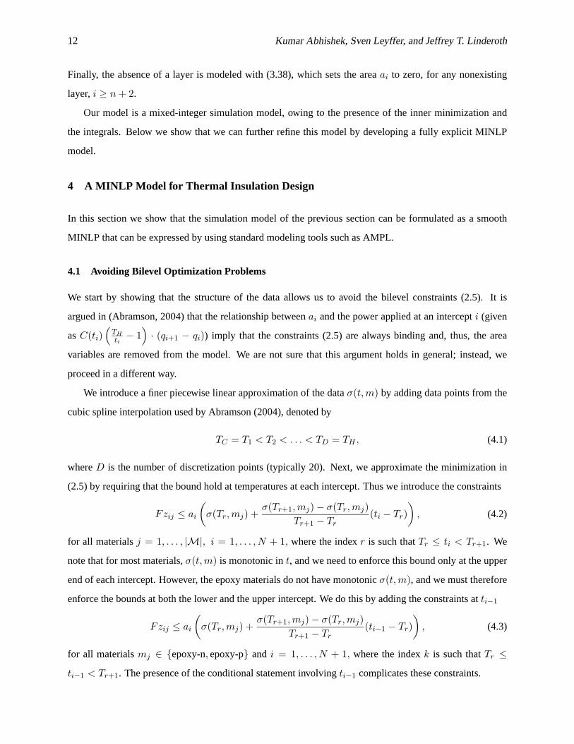
12 Kumar Abhishek, Sven Leyffer, and Jeffrey T. Linderoth
Finally, the absence of a layer is modeled with (3.38), which sets the areaai to zero, for any nonexisting
layer,i ≥ n + 2.
Our model is a mixed-integer simulation model, owing to the presence of the inner minimization and
the integrals. Below we show that we can further refine this model by developing a fully explicit MINLP
model.
4 A MINLP Model for Thermal Insulation Design
In this section we show that the simulation model of the previous section can be formulated as a smooth
MINLP that can be expressed by using standard modeling tools such as AMPL.
4.1 Avoiding Bilevel Optimization Problems
We start by showing that the structure of the data allows us to avoid the bilevelconstraints (2.5). It is
argued in (Abramson, 2004) that the relationship betweenai and the power applied at an intercepti (given
asC(ti)(
TH
ti− 1
)
· (qi+1 − qi)) imply that the constraints (2.5) are always binding and, thus, the area
variables are removed from the model. We are not sure that this argument holds in general; instead, we
proceed in a different way.
We introduce a finer piecewise linear approximation of the dataσ(t, m) by adding data points from the
cubic spline interpolation used by Abramson (2004), denoted by
TC = T1 < T2 < . . . < TD = TH , (4.1)
whereD is the number of discretization points (typically 20). Next, we approximate the minimization in
(2.5) by requiring that the bound hold at temperatures at each intercept. Thus we introduce the constraints
Fzij ≤ ai
(
σ(Tr, mj) +σ(Tr+1, mj) − σ(Tr, mj)
Tr+1 − Tr
(ti − Tr)
)
, (4.2)
for all materialsj = 1, . . . , |M|, i = 1, . . . , N + 1, where the indexr is such thatTr ≤ ti < Tr+1. We
note that for most materials,σ(t, m) is monotonic int, and we need to enforce this bound only at the upper
end of each intercept. However, the epoxy materials do not have monotonicσ(t, m), and we must therefore
enforce the bounds at both the lower and the upper intercept. We do this byadding the constraints atti−1
Fzij ≤ ai
(
σ(Tr, mj) +σ(Tr+1, mj) − σ(Tr, mj)
Tr+1 − Tr
(ti−1 − Tr)
)
, (4.3)
for all materialsmj ∈ {epoxy-n, epoxy-p} and i = 1, . . . , N + 1, where the indexk is such thatTr ≤
ti−1 < Tr+1. The presence of the conditional statement involvingti−1 complicates these constraints.
Modeling without Categorical Variables: A MINLP Model for Thermal Insulation Systems 13
A convenient way to model the conditional relationshipTr ≤ ti−1 ≤ Tr+1 in (4.2) is as the following
summation.
Fzij ≤ ai
D∑
r=1
Tr≤ti−1≤Tr+1
(
σ(Tr, mj) +σ(Tr+1, mj) − σ(Tr, mj)
Tr+1 − Tr
(ti − Tr)
)
. (4.4)
Similarly, we replace (4.3) by
Fzij ≤ ai ≤
D∑
r=1
Tr≤ti−1≤Tr+1
(
σ(Tr, mj) +σ(Tr+1, mj) − σ(Tr, mj)
Tr+1 − Tr
(ti−1 − Tr)
)
. (4.5)
We note that only a single term in this summation will be active. The resulting constraint is continuous but
not smooth, asti passes through the breakpoints. However, this nonsmoothness does notappear to cause
any problems for the NLP solvers. In Section 5 we provide a reformulation of these nonsmooth constraints
that employs integer variables and a finer discretization ofTr.
4.2 Evaluation of Integrals
The model involves integrals over the data functionsk(t, m) andk(t, m) · e(t, m) in (2.3) and (2.7). In
(Abramson, 2004) these integrals are evaluated by using Simpson’s rule,which is consistent with the piece-
wise cubic spline interpolation of the data. However, Simpson’s rule adds nonlinearity and would be difficult
to implement in a modeling language. Instead, we add more data points consistentwith the cubic spline in-
terpolation as in (4.1), and we evaluate the integrals using the trapezoidal rule on the data points
(Tr, k(Tr, mj)) and (Tr, k(Tr, mj) · e(Tr, mj)) .
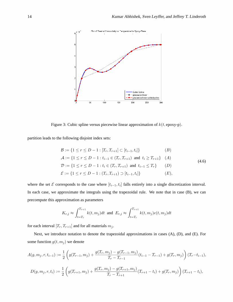
We note that adding more data points does not increase the number of variables in the model and greatly
reduces the nonlinearity of the constraints, without sacrificing accuracy, as can be seen from Figure 3,
which shows the cubic spline versus the piecewise linear approximation ofk(t, epoxy-p). The additional
data points clearly improve the fidelity of the piecewise linear approximation, as can be seen from the dotted
line that represents a piecewise linear interpolation of the original data points.
In general, the temperatures at the intercepts,ti will not take the values used in the discretization,Tr,
which we must take into account when calculating the values of the integrals. Figure 4 illustrates our
approach. For a given integration range[ti−1, ti], we split the integral into three distinct areas (A, B, and D
in Figure 4) depending on the relative position of the variablesti−1, ti and the discretization pointsTr. This
14 Kumar Abhishek, Sven Leyffer, and Jeffrey T. Linderoth
Figure 3: Cubic spline versus piecewise linear approximation ofk(t, epoxy-p).
partition leads to the following disjoint index sets:
B := {1 ≤ r ≤ D − 1 : [Tr, Tr+1] ⊂ [ti−1, ti]} (B)
A := {1 ≤ r ≤ D − 1 : ti−1 ∈ (Tr, Tr+1) and ti ≥ Tr+1} (A)
D := {1 ≤ r ≤ D − 1 : ti ∈ (Tr, Tr+1) and ti−1 ≤ Tr} (D)
E := {1 ≤ r ≤ D − 1 : (Tr, Tr+1) ⊃ [ti−1, ti]} (E),
(4.6)
where the setE corresponds to the case where[ti−1, ti] falls entirely into a single discretization interval.
In each case, we approximate the integrals using the trapezoidal rule. We note that in case (B), we can
precompute this approximation as parameters
Kr,j ≈
∫ Tr+1
t=Tr
k(t, mj)dt and Er,j ≈
∫ Tr+1
t=Tr
k(t, mj)e(t, mj)dt
for each interval[Tr, Tr+1] and for all materialsmj .
Next, we introduce notation to denote the trapezoidal approximations in cases(A), (D), and (E). For
some functiong(t, mj) we denote
A(g, mj , r, ti−1) :=1
2
(
g(Tr−1, mj) +g(Tr, mj) − g(Tr−1, mj)
Tr − Tr−1(ti−1 − Tr−1) + g(Tr, mj)
)
(Tr−ti−1),
D(g, mj , r, ti) :=1
2
(
g(Tr+1, mj) +g(Tr, mj) − g(Tr+1, mj)
Tr − Tr+1(Tr+1 − ti) + g(Tr, mj)
)
(Tr+1 − ti),

Modeling without Categorical Variables: A MINLP Model for Thermal Insulation Systems 15
AB
k(t,m)
t
D
t ti−1 i
Tr Tr+1
Figure 4: Illustration of the integral computation.
and
E(g, mj , r, ti) := 12
(
g(Tr, mj) +g(Tr+1,mj)−g(Tr,mj)
Tr+1−Tr(ti−1 − Tr)
+g(Tr, mj) +g(Tr+1,mj)−g(Tr,mj)
Tr+1−Tr(ti − Tr) + g(Tr, mj)
)
(Ti − ti−1)
as the trapezoidal approximation in the areas identified by the setsA, D, andE , respectively. Introducing
variablesvij andwij that approximate
vij ≈
∫ ti
ti−1
k(t, mj)dt, wij ≈
∫ ti
ti−1
k(t, mj)e(t, mj)dt,
we can expressvij andwij as
vij =∑
r∈B
Kr,j +∑
r∈A
A(k, mj , r, ti−1) +∑
r∈D
D(k, mj , r, ti) +∑
r∈E
E(k, mj , r, ti) (4.7)
and
wij =∑
r∈B
Er,j +∑
r∈A
A(k · e, mj , r, ti−1) +∑
r∈D
D(k · e, mj , r, ti) +∑
r∈E
E(k · e, mj , r, ti). (4.8)
The introduction ofvij , wij allows us to formulate the load-bearing thermal insulation design MVP as a
standard MINLP. Before proceeding, however, we simplify some of the nonlinear expressions further to
avoid division by zero that can confound standard NLP software. Thus, we rewrite (2.3) as
qixi = ai
|M|∑
j=1
zijvij , i = 1, . . . , N + 1. (4.9)
We introduce a new variableui = ∆xi/xi to model the thermal expansion of each layer, and we rewrite
(2.7) as
ui
|M|∑
j=1
zijvij =
|M|∑
j=1
zijwij , i = 1, . . . , N + 1. (4.10)
16 Kumar Abhishek, Sven Leyffer, and Jeffrey T. Linderoth
Thus, we can write (3.30) asN+1∑
i=1
uixi ≤ Lδ
100. (4.11)
This reformulation removes the categorical variablesm ∈ M from the model and leaves us with a standard
MINLP given as follows.
minimizeN+1∑
i=1
qiyi
(
C(ti−1)(TH
ti−1− 1) − C(ti)(
TH
ti− 1)
)
:= CoolingPower
subject to (3.13), (3.14), (3.16), (3.25), (3.32), (3.28), (3.33)
(3.37), (3.35), (3.38), (4.9), (4.10), (4.11)
(4.4), (4.7), (4.8), ∀j = 1, . . . , |M|, i = 1, . . . , N + 1
(4.5), ∀mj ∈ {epoxy-n, epoxy-p}, i = 1, . . . , N + 1 (P-0)
t0 = TC and tN+1 = TH
yi ∈ {0, 1}, ∀i = 1, . . . , N + 1
zij ∈ {0, 1}, ∀i = 1, . . . , N + 1, j = 1, . . . , |M|
xi, qi, ui, vij , wij , n, ti, ai ∈ R
We note that this model contains discontinuous objective coefficients. Next,we show how to reformulate
these discontinuous objective coefficients to arrive at a smoother MINLP.
4.3 Modeling a Discontinuous Function with Binary Variables
The discontinuous thermodynamic cycle efficiency coefficientC(ti) in (2.1) can be replaced by a smooth
relationship. We start by introducing additional binary variablesski ∈ {0, 1}, k = 1, . . . , 3 to model the
following implications.
ti ≤ 4.2 ⇒ s1i = 1 (4.12)
4.2 < ti < 71 ⇒ s2i = 1 (4.13)
ti ≥ 71 ⇒ s3i = 1 (4.14)
Letting ε > 0 be a small constant that models the strict inequalities in (2.1), we can model the implications
(4.12) and (4.14) as
ti − (TC − 4.2 − ε)s1i ≥ 4.2 + ε (4.15)
ti − (TH − 71 + ε)s3i ≤ 71 − ε, (4.16)
Modeling without Categorical Variables: A MINLP Model for Thermal Insulation Systems 17
respectively. Condition (4.13) is equivalent to
s2i = 0 ⇒ ti ≤ 4.2 or ti ≥ 71,
which we model as follows:
s1i + s2i + s3i = 1 (4.17)
ti + (TH − 4.2)s1i ≤ TH (4.18)
ti − (71 − TC)si3 ≥ TC . (4.19)
Equation (4.17) models the implication that eachti is in exactly one interval. The two inequalities (4.18)
and (4.19) fixsik ∈ {0, 1} given anyti, and constrainti for any valid choice ofsik ∈ {0, 1}. The approach
presented here is fairly general and applies to other piecewise functionsas well.
4.4 A Piecewise Smooth MINLP Model
The smooth MINLP model is now given as follows.
minimizeN+1∑
i=1
qiyi
(
(5s1,i−1 + 4s2,i−1 + 2.5s3,i−1)
(
TH
ti−1− 1
)
−(5s1i + 4s2i + 2.5s3i)
(
TH
ti− 1
))
:= CoolingPower
subject to (3.13), (3.14), (3.16), (3.25), (3.32), (3.28), (3.33)
(3.37), (3.35), (3.38), (4.9), (4.10), (4.11)
(4.7), (4.8), (4.4), ∀j = 1, . . . , |M|, i = 1, . . . , N + 1
(4.5), ∀mj ∈ {epoxy-n, epoxy-p}, i = 1, . . . , N + 1 (P-1)
(4.15), (4.16), (4.17), (4.18), (4.19), ∀i = 1, . . . , N + 1
t0 = TC and tN+1 = TH
yi ∈ {0, 1}, ∀i = 1, . . . , N + 1
zij ∈ {0, 1}, ∀i = 1, . . . , N + 1, j = 1, . . . , |M|,
ski ∈ {0, 1}, ∀i = 1, . . . , N + 1, k = 1, . . . , 3
xi, qi, ui, vij , wij , n, ti, ai ∈ R
When we ran this model, we noticed that the objective functionCoolingPower can become negative,
which is a nonphysical solution. More specifically, solving a relaxation of (P-1) at a node in a branch-and-
bound procedure can yield a negative solution. The reason for this behavior is that the variablesski now

18 Kumar Abhishek, Sven Leyffer, and Jeffrey T. Linderoth
have fractional values, and thus the differences(
(5s1,i−1 + 4s2,i−1 + 2.5s3,i−1)
(
TH
ti−1− 1
)
− (5s1i + 4s2i + 2.5s3i)
(
TH
ti− 1
))
∀i = 1, . . . , N +1
(4.20)
need not be non-negative. Thus we add the constraintCoolingPower >= 0 to the models.
We note that model (P-1) is nonsmooth as a result of the presence of conditional statements in constraints
(4.4), (4.5), (4.7), and (4.8), which include summations that depend on thetemperatureti. These nonsmooth
constraints may cause trouble for standard NLP solvers. We show in Section 6 that we can solve such models
despite the presence of nonsmooth equations.
5 A Smooth MINLP Model with Discretized Temperature
In this section we describe an alternative formulation of the thermal insulation model that assumes that we
select the temperatures at the intercepts,ti from a discrete set (4.1). This formulation may at first sight
seem more complicated, but it allows us to remove the nonsmoothness presentin model (P-1). We envisage
using a large number of discretization points (e.g. at one-degree level). This assumption may seem strong.
However, we note that we can always use the discrete values ofti to discover the optimal value of the
structure variables,n andmi ∈ M and then run an NLP to adjust the temperatures and thickness of the final
design. This simplification is justified by the fact that the solution of a MINLP is typically more sensitive to
the choice of the integer variables than to the choice of the continuous variables.
As before, we model the discrete choice of temperatures by introducing SOS-1 variables,
ti =D
∑
r=1
dirTr, 1 =D
∑
r=1
dir, dir ∈ {0, 1}, ∀i = 0, . . . , N + 1, (5.1)
wheredir = 1 if intercepti is kept at temperatureTr, and0 otherwise. We note that the new variablesdir are
a SOS-1, and so we need to go only to at mostlog(D) branching levels in the tree, making this an efficient
reformulation.
Introducing a discrete set of temperatures simplifies the MINLP model in a number of ways. We start by
simplifying constraints (4.7) and (4.8). We precompute the integrals ofk(t, mj) andk(t, mj)e(t, mj) over
[T1, Tr] as fixed parameters:
Vrj ≈
∫ Tr
T1
k(t, mj)dt and Wrj ≈
∫ Tr
T1
k(t, mj)e(t, mj)dt
for all r = 1, . . . , D andj = 1, . . . , |M|. Next, we use the identity
vij =
∫ ti
t=ti−1
k(t, mj)dt =
∫ ti
t=T1
k(t, mj)dt −
∫ ti−1
t=T1
k(t, mj)dt
Modeling without Categorical Variables: A MINLP Model for Thermal Insulation Systems 19
and observe that (5.1) implies
∫ ti
t=T1
k(t, mj)dt =D
∑
r=1
dir
∫ Tr
t=T1
k(t, mj)dt.
Thus, equations (4.7) and (4.8) simplify to the following set oflinear equations:
vij =D
∑
r=1
dirVrj −D
∑
r=1
di−1,rVrj ∀i = 0, . . . , N, j = 1, . . . , |M|, (5.2)
wij =D
∑
r=1
dirWrj −D
∑
r=1
di−1,rWrj ∀i = 0, . . . , N, j = 1, . . . , |M|. (5.3)
Next, we show how (5.1) simplifies the objective function. First, we observethat
(
TH
ti− 1
)
=
(
TH∑D
r=1 dirTr
− 1
)
=
(
D∑
r=1
dirTH
Tr
− 1
)
. (5.4)
We can replace the binary variablessik modeling the discontinuous objective coefficients by defining con-
stants
Cr :=
5 if Tr ≤ 4.2
4 if 4.2K < Tr < 71K ,
2.5 if Tr ≥ 71K
(5.5)
which replaceC(ti) in the objective function. Combining (5.4) and (5.5), we reformulate the objective
function asN+1∑
i=1
qi
(
D∑
r=1
(di−1,r − dir)Cr
(
TH
Tr
− 1
)
)
:= CoolingPower.
The constraints that bound the temperature difference between consecutive layers, (3.35), can be ex-
pressed as binary inequalities betweendir anddi−1,r:
D∑
r=1
rdir ≥D
∑
r=1
rdi−1,r + yi, ∀i = 1, . . . , N + 1, (5.6)
which implies thatti > ti−1 by at least one discretization difference. Similarly, we can express constraints
(3.37) as a discrete set of constraints:
diD ≥ (1 − yi+1), ∀i = 1, . . . , N. (5.7)
We next simplify the area stress constraints (4.4) and (4.5). We start by rewriting the bilevel constraint
(2.5) as an infinite set of constraints:
F ≤ aiσ(t, mi), ∀t ∈ [ti−1, ti], ∀i = 1, . . . , N + 1.
20 Kumar Abhishek, Sven Leyffer, and Jeffrey T. Linderoth
We observe that the discrete range of the temperature variable allows us to formulate this constraint as a
finite set of inequalities:
F ≤ aiσ(Ts, mi), ∀s : ti−1 ≤ Ts ≤ ti, ∀i = 1, . . . , N + 1.
We introduce the tensile yield strengthσsj := σ(Ts, mj) of each material at all discrete temperature values
to remove the dependence on the categorical variablemi:
F ≤ ai
|M|∑
j=1
zijσsj , ∀s : ti−1 ≤ Ts ≤ ti, ∀i = 1, . . . , N + 1.
We formulate the conditions : ti−1 ≤ Ts ≤ ti using the SOS variablesdir as follows. First, we introduce
the following partial sums for notational convenience:
pis :=s
∑
r=1
di−1,r −s−1∑
r=1
dir =
1 if s : ti−1 ≤ Ts ≤ ti
0 else,
which follows from (5.1). Thus, we can write (2.5) as
F ≤ ai
|M|∑
j=1
zijσsj + (1 − pis)Fmax ∀s = 1, . . . , D − 1 ∀i = 1, . . . , N + 1, (5.8)
whereFmax is an upper bound onF .
We can further tighten the formulation by modeling the implications
dir = 1 ⇒D
∑
s=r
dj,s = 0 ∀j = 1 . . . i − 1, i = 1 . . . N + 1, r = 1 . . . D
dir = 1 ⇒r
∑
s=1
dj,s = 0 ∀j = i + 1 . . . N + 1, i = 1 . . . N + 1, r = 1 . . . D,
which is modeled as the valid inequalities
i−1∑
j=1
D∑
s=r
djs +N+1∑
j=i+1
r∑
s=1
dj,s ≤ B(1 − dir) ∀i = 1 . . . N + 1, r = 1 . . . D, (5.9)
whereB ≡ 2N is an upper bound on the left-hand side of the inequality.
The resulting model is a smooth MINLP, to which standard MINLP solution techniques can now be
Modeling without Categorical Variables: A MINLP Model for Thermal Insulation Systems 21
applied to find a local solution.
minimizeN+1∑
i=1
qi
(
D∑
r=1
(di−1,r − dir)Cr
(
TH
Tr
− 1
)
)
:= CoolingPower
subject to (3.13), (3.14), (3.16), (3.25), (3.32), (3.28), (3.33)
(3.38), (4.9), (4.10), (4.11)
(5.1), (5.2), (5.3)
(5.6), (5.7), (5.8), (5.9) (P-2)
t0 = TC and tN+1 = TH
yi ∈ {0, 1}, ∀i = 1, . . . , N + 1
zij ∈ {0, 1}, ∀i = 1, . . . , N + 1, j = 1, . . . , |M|,
dir ∈ {0, 1}, ∀i = 1, . . . , N + 1, r = 1, . . . , D,
xi, qi, ui, vij , wij , n, ti, ai ∈ R
Model (P-2) has fewer nonlinear constraints than either (P-0) or (P-1) and is a smooth MINLP. On the
other hand, the additional SOS-1 variablesdir make the model larger.
6 Solution Methodology and Computational Results
We have experimented with three models with different smoothness properties. All models are available in
AMPL (Fourer et al., 2003) from the authors upon request. The main characteristics of the three models for
N = 10 are summarized in Table 4. The problem size is roughly linear inN , and the model withN = 20
has about twice as many variables and constraints as the model withN = 10.
Table 4: Comparison of MINLP Models forN = 10
# Variables # Constraints
Model (bin/SOS/int/cont) (nonlinear/linear) Smoothness
MVP discontinuous objective & constraints
(P-0) 144 (88/0/1/45) 212 (115/97) discontinuous objective
(P-1) 174 (118/0/1/55) 262 (115/147) nonsmooth constraints
(P-2) 3696 (3596/11/1/99) 6715 (3281/3434) smooth as a whistle
We employ standard solution techniques for the solution of the MINLP models (P-0), (P-1), and (P-2)
22 Kumar Abhishek, Sven Leyffer, and Jeffrey T. Linderoth
such as branch-and-bound method (Dakin, 1965; Gupta and Ravindran, 1985), and the LP/NLP-based branch-
and-bound method (Quesada and Grossmann, 1992); see Grossmann (2002) for a recent survey of solution
techniques for MINLP problems.
We note that the models (P-0), (P-1), and (P-2) are nonconvex, makingit hard to solve these models to
global optimality. We employ a standard nonlinear branch-and-bound-based solver, MINLP-BB (Leyffer,
1998), for solving these models. The main idea behind branch-and-bound is to solve continuous relaxations
of the original problem and to divide the feasible region, eliminating the fractional solution of relaxed
problem. Continuing in this manner yields a tree of problems that is searched for the integer optimum.
The NLP subproblem solved at a node provides a valid lower bound for the subproblems in the descendant
nodes. An integer feasible solution when found provides an upper bound for the problem.
We resort to the strategy of multistarts for solving the nonconvex models (P-0) and (P-1). The strategy
of multistarts involves solving a problem at a node a number of times from various starting points. For every
node of the branch-and-bound tree, we store a logical switch that indicates whether to perform multiple
starts. Initially, this switch is set to true, and we performR(= 5) restarts from randomly generated starting
points and select the best solution value obtained as the solution of that node. If all runs give the same
solution value, then we set the logical switch to false for this node and for allits children. Otherwise, the
switch remains true for all child nodes. Thus, for convex problems, we perform a multistart only at the root
node.
We also set priorities on the integer variables in the model for MINLP-BB to perform branching. For the
model (P-0), the integer variablen is given the highest priority, so that the solver branches on a fractional
value of the variablen, before branching on other variables. The variablesyi have the next highest priority,
since they are dependent onn. The variables for the choice of materials,zik are accorded the next highest
priority, since they are dependent on bothn andyi. For the model (P-1), the variables for the discontinuous
objective coefficients,sik are given the least priority.
We ran these models on a Beowulf cluster of computers consisting of 120 nodes of 64-bit AMD Opteron
microprocessors. Each of the nodes has a CPU clockspeed of 1.8 GHz,has 2 GB RAM, and runs on the
Fedore Core 2 operating system. The models were run without any time limits, with the aim of letting the
branch-and-bound enumeration run to completion. For the model (P-0), we did two different runs, choosing
the parameterN , the maximum number of intercepts in the system, to be10 and20. The results of the runs
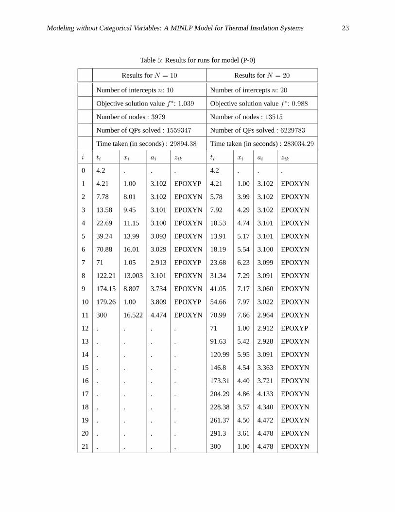
for N = 10 andN = 20 are summarized in Table 5. By increasing the number of intercepts, we are able
to improve the solution obtained by Abramson (2004) from1.0623 to 1.039 and0.988 for N = 10 and
N = 20, respectively.
Modeling without Categorical Variables: A MINLP Model for Thermal Insulation Systems 23
Table 5: Results for runs for model (P-0)
Results forN = 10 Results forN = 20
Number of interceptsn: 10 Number of interceptsn: 20
Objective solution valuef∗: 1.039 Objective solution valuef∗: 0.988
Number of nodes :3979 Number of nodes :13515
Number of QPs solved :1559347 Number of QPs solved :6229783
Time taken (in seconds) :29894.38 Time taken (in seconds) :283034.29
i ti xi ai zik ti xi ai zik
0 4.2 . . . 4.2 . . .
1 4.21 1.00 3.102 EPOXYP 4.21 1.00 3.102 EPOXYN
2 7.78 8.01 3.102 EPOXYN 5.78 3.99 3.102 EPOXYN
3 13.58 9.45 3.101 EPOXYN 7.92 4.29 3.102 EPOXYN
4 22.69 11.15 3.100 EPOXYN 10.53 4.74 3.101 EPOXYN
5 39.24 13.99 3.093 EPOXYN 13.91 5.17 3.101 EPOXYN
6 70.88 16.01 3.029 EPOXYN 18.19 5.54 3.100 EPOXYN
7 71 1.05 2.913 EPOXYP 23.68 6.23 3.099 EPOXYN
8 122.21 13.003 3.101 EPOXYN 31.34 7.29 3.091 EPOXYN
9 174.15 8.807 3.734 EPOXYN 41.05 7.17 3.060 EPOXYN
10 179.26 1.00 3.809 EPOXYP 54.66 7.97 3.022 EPOXYN
11 300 16.522 4.474 EPOXYN 70.99 7.66 2.964 EPOXYN
12 . . . . 71 1.00 2.912 EPOXYP
13 . . . . 91.63 5.42 2.928 EPOXYN
14 . . . . 120.99 5.95 3.091 EPOXYN
15 . . . . 146.8 4.54 3.363 EPOXYN
16 . . . . 173.31 4.40 3.721 EPOXYN
17 . . . . 204.29 4.86 4.133 EPOXYN
18 . . . . 228.38 3.57 4.340 EPOXYN
19 . . . . 261.37 4.50 4.472 EPOXYN
20 . . . . 291.3 3.61 4.478 EPOXYN
21 . . . . 300 1.00 4.478 EPOXYN
24 Kumar Abhishek, Sven Leyffer, and Jeffrey T. Linderoth
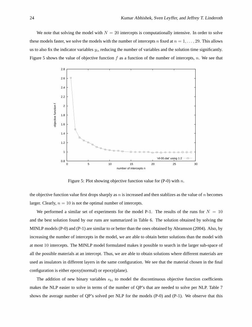
We note that solving the model withN = 20 intercepts is computationally intensive. In order to solve
these models faster, we solve the models with the number of interceptsn fixed atn = 1, . . . , 29. This allows
us to also fix the indicator variablesyi, reducing the number of variables and the solution time significantly.
Figure 5 shows the value of objective functionf as a function of the number of intercepts,n. We see that
0.8
1
1.2
1.4
1.6
1.8
2
2.2
2.4
2.6
2.8
0 5 10 15 20 25 30
obje
ctiv
e fu
nctio
n f
number of intercepts n
’nf-00.dat’ using 1:2
Figure 5: Plot showing objective function value for (P-0) withn.
the objective function value first drops sharply asn is increased and then stablizes as the value ofn becomes
larger. Clearly,n = 10 is not the optimal number of intercepts.
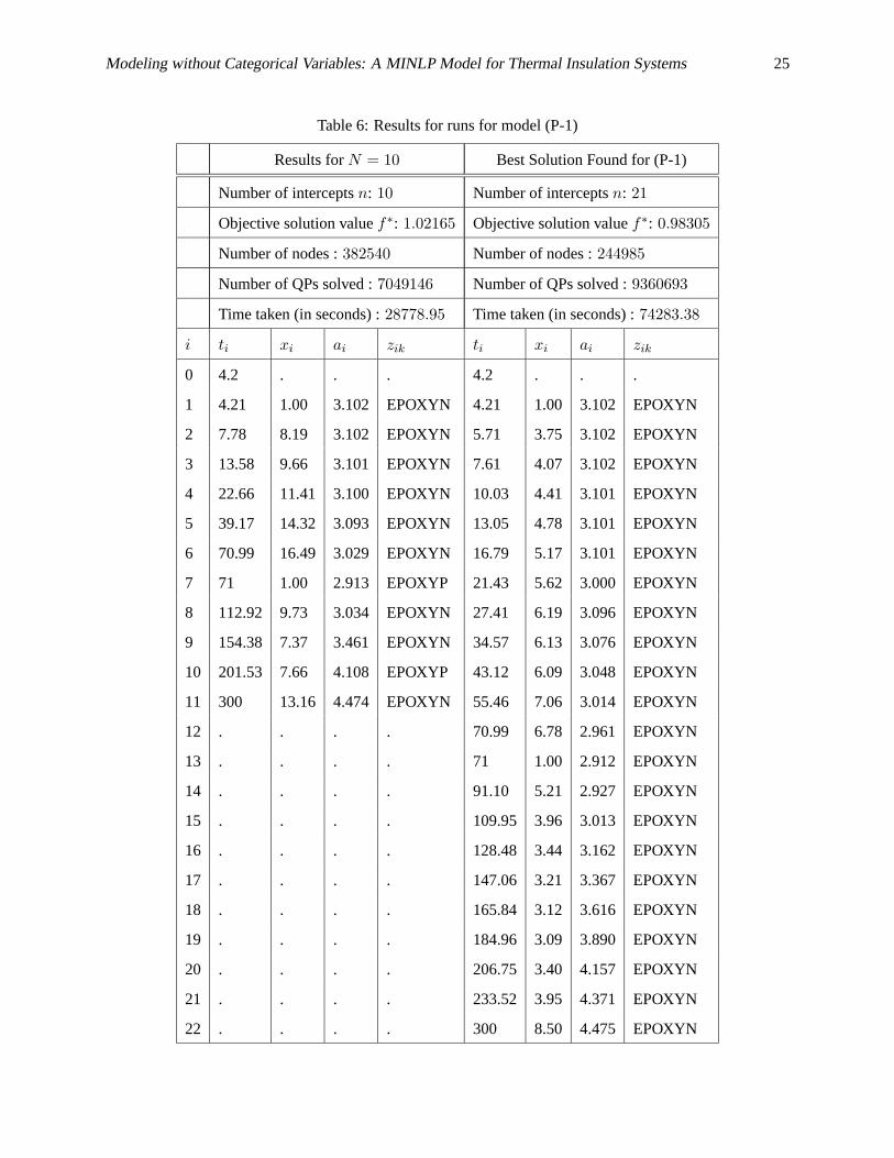
We performed a similar set of experiments for the model P-1. The results of the runs forN = 10
and the best solution found by our runs are summarized in Table 6. The solution obtained by solving the
MINLP models (P-0) and (P-1) are similar to or better than the ones obtained by Abramson (2004). Also, by
increasing the number of intercepts in the model, we are able to obtain better solutions than the model with
at most10 intercepts. The MINLP model formulated makes it possible to search in the larger sub-space of
all the possible materials at an intercept. Thus, we are able to obtain solutions where different materials are
used as insulators in different layers in the same configuration. We see that the material chosen in the final
configuration is either epoxy(normal) or epoxy(plane).
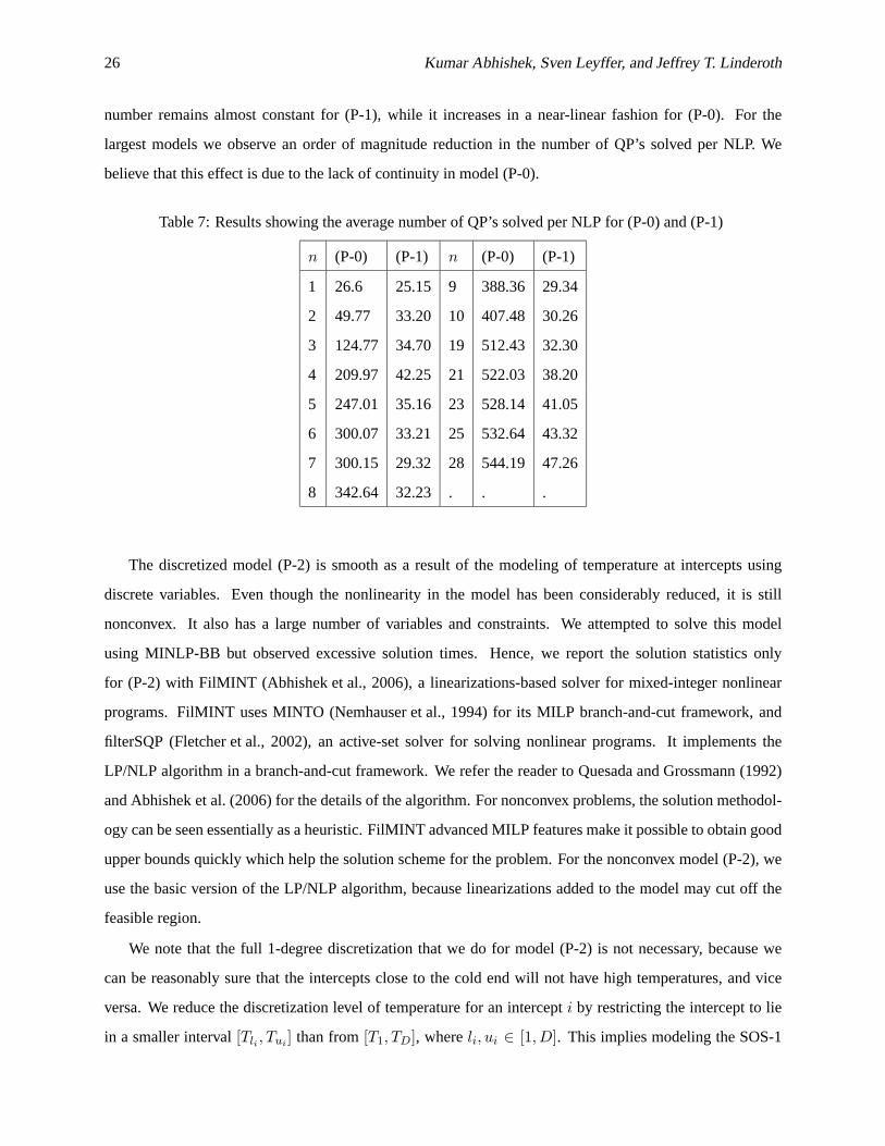
The addition of new binary variablesski to model the discontinuous objective function coefficients
makes the NLP easier to solve in terms of the number of QP’s that are needed tosolve per NLP. Table 7
shows the average number of QP’s solved per NLP for the models (P-0) and (P-1). We observe that this
Modeling without Categorical Variables: A MINLP Model for Thermal Insulation Systems 25
Table 6: Results for runs for model (P-1)
Results forN = 10 Best Solution Found for (P-1)
Number of interceptsn: 10 Number of interceptsn: 21
Objective solution valuef∗: 1.02165 Objective solution valuef∗: 0.98305
Number of nodes :382540 Number of nodes :244985
Number of QPs solved :7049146 Number of QPs solved :9360693
Time taken (in seconds) :28778.95 Time taken (in seconds) :74283.38
i ti xi ai zik ti xi ai zik
0 4.2 . . . 4.2 . . .
1 4.21 1.00 3.102 EPOXYN 4.21 1.00 3.102 EPOXYN
2 7.78 8.19 3.102 EPOXYN 5.71 3.75 3.102 EPOXYN
3 13.58 9.66 3.101 EPOXYN 7.61 4.07 3.102 EPOXYN
4 22.66 11.41 3.100 EPOXYN 10.03 4.41 3.101 EPOXYN
5 39.17 14.32 3.093 EPOXYN 13.05 4.78 3.101 EPOXYN
6 70.99 16.49 3.029 EPOXYN 16.79 5.17 3.101 EPOXYN
7 71 1.00 2.913 EPOXYP 21.43 5.62 3.000 EPOXYN
8 112.92 9.73 3.034 EPOXYN 27.41 6.19 3.096 EPOXYN
9 154.38 7.37 3.461 EPOXYN 34.57 6.13 3.076 EPOXYN
10 201.53 7.66 4.108 EPOXYP 43.12 6.09 3.048 EPOXYN
11 300 13.16 4.474 EPOXYN 55.46 7.06 3.014 EPOXYN
12 . . . . 70.99 6.78 2.961 EPOXYN
13 . . . . 71 1.00 2.912 EPOXYN
14 . . . . 91.10 5.21 2.927 EPOXYN
15 . . . . 109.95 3.96 3.013 EPOXYN
16 . . . . 128.48 3.44 3.162 EPOXYN
17 . . . . 147.06 3.21 3.367 EPOXYN
18 . . . . 165.84 3.12 3.616 EPOXYN
19 . . . . 184.96 3.09 3.890 EPOXYN
20 . . . . 206.75 3.40 4.157 EPOXYN
21 . . . . 233.52 3.95 4.371 EPOXYN
22 . . . . 300 8.50 4.475 EPOXYN
26 Kumar Abhishek, Sven Leyffer, and Jeffrey T. Linderoth
number remains almost constant for (P-1), while it increases in a near-linear fashion for (P-0). For the
largest models we observe an order of magnitude reduction in the number ofQP’s solved per NLP. We
believe that this effect is due to the lack of continuity in model (P-0).
Table 7: Results showing the average number of QP’s solved per NLP for(P-0) and (P-1)
n (P-0) (P-1) n (P-0) (P-1)
1 26.6 25.15 9 388.36 29.34
2 49.77 33.20 10 407.48 30.26
3 124.77 34.70 19 512.43 32.30
4 209.97 42.25 21 522.03 38.20
5 247.01 35.16 23 528.14 41.05
6 300.07 33.21 25 532.64 43.32
7 300.15 29.32 28 544.19 47.26
8 342.64 32.23 . . .
The discretized model (P-2) is smooth as a result of the modeling of temperature at intercepts using
discrete variables. Even though the nonlinearity in the model has been considerably reduced, it is still
nonconvex. It also has a large number of variables and constraints. Weattempted to solve this model
using MINLP-BB but observed excessive solution times. Hence, we report the solution statistics only
for (P-2) with FilMINT (Abhishek et al., 2006), a linearizations-based solver for mixed-integer nonlinear
programs. FilMINT uses MINTO (Nemhauser et al., 1994) for its MILP branch-and-cut framework, and
filterSQP (Fletcher et al., 2002), an active-set solver for solving nonlinear programs. It implements the
LP/NLP algorithm in a branch-and-cut framework. We refer the readerto Quesada and Grossmann (1992)
and Abhishek et al. (2006) for the details of the algorithm. For nonconvexproblems, the solution methodol-
ogy can be seen essentially as a heuristic. FilMINT advanced MILP features make it possible to obtain good
upper bounds quickly which help the solution scheme for the problem. For thenonconvex model (P-2), we
use the basic version of the LP/NLP algorithm, because linearizations addedto the model may cut off the
feasible region.
We note that the full 1-degree discretization that we do for model (P-2) is not necessary, because we
can be reasonably sure that the intercepts close to the cold end will not have high temperatures, and vice
versa. We reduce the discretization level of temperature for an intercepti by restricting the intercept to lie
in a smaller interval[Tli , Tui] than from[T1, TD], whereli, ui ∈ [1, D]. This implies modeling the SOS-1
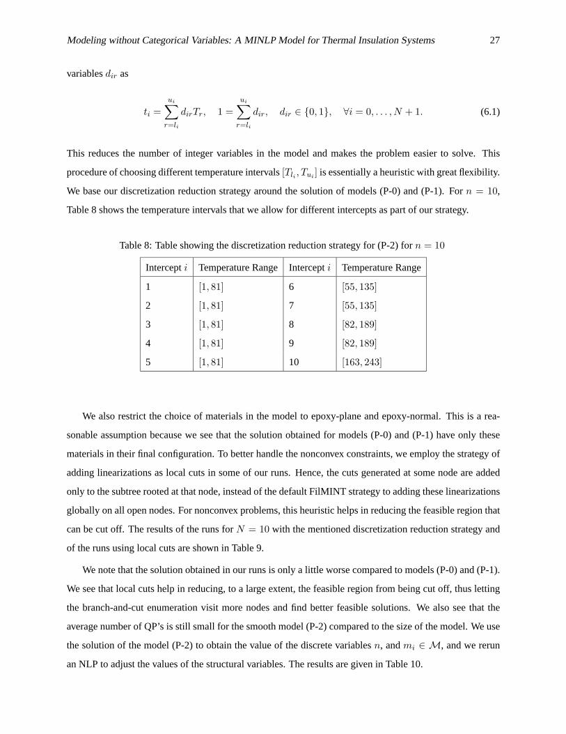
Modeling without Categorical Variables: A MINLP Model for Thermal Insulation Systems 27
variablesdir as
ti =
ui∑
r=li
dirTr, 1 =
ui∑
r=li
dir, dir ∈ {0, 1}, ∀i = 0, . . . , N + 1. (6.1)
This reduces the number of integer variables in the model and makes the problem easier to solve. This
procedure of choosing different temperature intervals[Tli , Tui] is essentially a heuristic with great flexibility.
We base our discretization reduction strategy around the solution of models (P-0) and (P-1). Forn = 10,
Table 8 shows the temperature intervals that we allow for different intercepts as part of our strategy.
Table 8: Table showing the discretization reduction strategy for (P-2) forn = 10
Intercepti Temperature RangeIntercepti Temperature Range
1 [1, 81] 6 [55, 135]
2 [1, 81] 7 [55, 135]
3 [1, 81] 8 [82, 189]
4 [1, 81] 9 [82, 189]
5 [1, 81] 10 [163, 243]
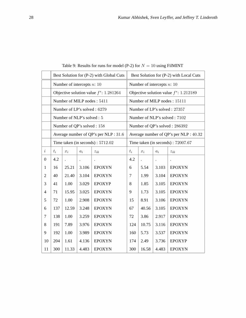
We also restrict the choice of materials in the model to epoxy-plane and epoxy-normal. This is a rea-
sonable assumption because we see that the solution obtained for models (P-0) and (P-1) have only these
materials in their final configuration. To better handle the nonconvex constraints, we employ the strategy of
adding linearizations as local cuts in some of our runs. Hence, the cuts generated at some node are added
only to the subtree rooted at that node, instead of the default FilMINT strategy to adding these linearizations
globally on all open nodes. For nonconvex problems, this heuristic helps inreducing the feasible region that
can be cut off. The results of the runs forN = 10 with the mentioned discretization reduction strategy and
of the runs using local cuts are shown in Table 9.
We note that the solution obtained in our runs is only a little worse compared to models (P-0) and (P-1).
We see that local cuts help in reducing, to a large extent, the feasible regionfrom being cut off, thus letting
the branch-and-cut enumeration visit more nodes and find better feasiblesolutions. We also see that the
average number of QP’s is still small for the smooth model (P-2) compared to the size of the model. We use
the solution of the model (P-2) to obtain the value of the discrete variablesn, andmi ∈ M, and we rerun
an NLP to adjust the values of the structural variables. The results are given in Table 10.
28 Kumar Abhishek, Sven Leyffer, and Jeffrey T. Linderoth
Table 9: Results for runs for model (P-2) forN = 10 using FilMINT
Best Solution for (P-2) with Global Cuts Best Solution for (P-2) with Local Cuts
Number of interceptsn: 10 Number of interceptsn: 10
Objective solution valuef∗: 1.281264 Objective solution valuef∗: 1.212189
Number of MILP nodes :5411 Number of MILP nodes :15111
Number of LP’s solved :6279 Number of LP’s solved :27357
Number of NLP’s solved :5 Number of NLP’s solved :7102
Number of QP’s solved :158 Number of QP’s solved :286392
Average number of QP’s per NLP :31.6 Average number of QP’s per NLP :40.32
Time taken (in seconds) :5712.02 Time taken (in seconds) :72007.67
i ti xi ai zik ti xi ai zik
0 4.2 . . . 4.2 . . .
1 16 25.21 3.106 EPOXYN 6 5.54 3.103 EPOXYN
2 40 21.40 3.104 EPOXYN 7 1.99 3.104 EPOXYN
3 41 1.00 3.029 EPOXYP 8 1.85 3.105 EPOXYN
4 71 15.95 3.025 EPOXYN 9 1.73 3.105 EPOXYN
5 72 1.00 2.908 EPOXYN 15 8.91 3.106 EPOXYN
6 137 12.59 3.248 EPOXYN 67 40.56 3.105 EPOXYN
7 138 1.00 3.259 EPOXYN 72 3.86 2.917 EPOXYN
8 191 7.89 3.976 EPOXYN 124 10.75 3.116 EPOXYN
9 192 1.00 3.989 EPOXYN 160 5.73 3.537 EPOXYN
10 204 1.61 4.136 EPOXYN 174 2.49 3.736 EPOXYP
11 300 11.33 4.483 EPOXYN 300 16.58 4.483 EPOXYN

Modeling without Categorical Variables: A MINLP Model for Thermal Insulation Systems 29
Table 10: Results for model (P-0) after fixing discrete variables using (P-2)
Results forn = 10
Objective Solution Valuef∗: 1.097219
Number of QPs Solved :508
i ti xi ai zik i ti xi ai zik
0 4.2 . . . 6 28.79 8.83 3.099 EPOXYN
1 4.21 1.01 3.102 EPOXYN 7 41.03 8.95 3.071 EPOXYN
2 6.44 5.09 3.106 EPOXYN 8 71 16.23 3.022 EPOXYN
3 9.59 5.70 3.102 EPOXYN 9 134.2 16.33 3.221 EPOXYN
4 13.91 6.38 3.101 EPOXYN 10 155.48 4.02 3.476 EPOXYP
5 19.75 7.13 3.100 EPOXYN 11 300 20.33 4.475 EPOXYN
7 Conclusions
We use mixed integer nonlinear programming techniques to model the load-bearing thermal insulation prob-
lem. We use integer variables to model the categorical variables, so that the model now allows continuous
relaxations and can be solved by using standard MINLP solution techniques. We develop facet-defining
inequalities for a relaxation of this reformulated MINLP model. We evaluate integrals by adding more data
points consistent with the cubic interpolation of the data and using trapezoidalrule. We also avoid the
second-level optimization in the problem by introducing a finer piecewise linear approximation of the data
and by enforcing the bounds at temperatures for each intercept.
Our reformulations give rise to three models with varying degrees of smoothness, and we comment on
the relative merits of the formulations. Our computational results indicate that theMINLP formulations
obtain better results than previous results by Abramson (2004). In particular, by increasing the number of
intercepts from10 to 20, we are able to reduce the cooling power by 4%.
The modeling of mixed variable problems as MINLPs allows us to apply more powerful techniques, such
as branch-and-bound, outer approximation, and branch-and-cut, rather than a heuristic search technique.
Engineering or modeling insight is included into the MILP model by using priorities on the integer variables
or by restricting temperature ranges for the intercepts. We believe that the modeling techniques shown here
are very general and can be used as a blueprint for modeling other design problems that have categorical
variables.
30 Kumar Abhishek, Sven Leyffer, and Jeffrey T. Linderoth
Acknowledgments
Much of this work was carried out while the first author was visiting Argonne through a student visitor
program, made possible through the support by the Mathematical, Information, and Computational Sciences
Division subprogram of the Office of Advanced Scientific Computing Research, Office of Science, U.S.
Department of Energy, under Contract DE-AC02-06CH11357. This work was also supported by the U.S.
Department of Energy through the grant DE-FG02-05ER25694.
References
Abhishek, K., Leyffer, S., and Linderoth, J. (2006). FilMINT: An outer approximation based nonlinear
mixed integer solver. Working Paper.
Abramson, M. A. (2004). Mixed variable optimization of a load-bearing thermal insulation system using a
filter pattern search algorithm.Optimization and Engineering, 5:157–177.
Abramson, M. A., Audet, C., and J. E. Dennis, J. (2004). Filter pattern search algorithms for mixed variable
constrained optimization problems. Technical Report TR04-09, CAAM, Rice University.
Audet, C. and Dennis, J. (2004). A pattern search filter method for nonlinear programming without deriva-
tives. SIAM J. Optimization, 14(4):980–1010.
Audet, C. and Dennis, J. E. (2000). Pattern search algorithms for mixed variable programming.SIAM J. on
Optimization, 11(3):573–594.
Beal, J. M., Shukla, A., Brezhneva, O. A., and Abramson, M. A. (2006). Optimal sensor placement for
enhancing sensitivity to change in stiffness for structural health monitoring. Technical report, Department
of Mathematics and Statistics, Air Force Institute of Technology.
Dakin, R. J. (1965). A tree search algorithm for mixed programming problems. Computer J., 8:250–255.
Fletcher, R., Leyffer, S., and Toint, P. (2002). On the global convergence of a Filter-SQP algorithm.SIAM
J. Optimization, 13:44–59.
Fourer, R., Gay, D. M., and Kernighan, B. W. (2003).AMPL: A Modelling Language for Mathematical
Programming. Books/Cole—Thomson Learning, 2nd edition.
Grossmann, I. E. (2002). Review of nonlinear mixed–integer and disjunctive programming techniques.
Optimization and Engineering, 3:227–252.
Modeling without Categorical Variables: A MINLP Model for Thermal Insulation Systems 31
Gupta, O. K. and Ravindran, A. (1985). Branch and bound experiments in convex nonlinear integer pro-
gramming.Management Science, 31:1533–1546.
Kokkolaras, M., Audet, C., and Dennis, J. E. (2001). Mixed variable optimization of the number and
composition of heat intercepts in a thermal insulation system.Optimization and Engineering, 2:5–29.
Leyffer, S. (1998). User manual for MINLP-BB. University of Dundee.
Nemhauser, G. and Wolsey, L. A. (1988).Integer and Combinatorial Optimization. John Wiley and Sons,
New York.
Nemhauser, G. L., Savelsbergh, M. W. P., and Sigismondi, G. C. (1994).MINTO, a Mixed INTeger Opti-
mizer. Operations Research Letters, 15:47–58.
Quesada, I. and Grossmann, I. E. (1992). An LP/NLP based branch–and–bound algorithm for convex
MINLP optimization problems.Computers and Chemical Engineering, 16:937–947.
Zhao, Z., Meza, J., and van Hove, M. (2005). Using pattern search methods for surface structure determi-
nation of nanostructures. Technical Report LBNL-57541, Lawrence Berkeley National Laboratory.
The submitted manuscript has been created by the UChicago Argonne, LLC, Operator of Argonne National Laboratory (“Argonne”) under Contract
No. DE-AC02-06CH11357 with the U.S. Department of Energy. The U.S. Government retains for itself, and others acting on itsbehalf, a paid-up,
nonexclusive, irrevocable worldwide license in said article to reproduce, prepare derivative works, distribute copies to the public, and perform
publicly and display publicly, by or on behalf of the Government.