modelling and assessing an efficient building with · modelling and assessing an efficient building...

2

Modelling and Assessing an Efficient Building with Absorption Chillier for Two Different Climates in M ENA

Region

By

Mohamad Jihad Almshkawi

A Thesis Submitted to Faculty of Engineering at Cairo University

and Faculty of Engineering at Kassel University

in Partial Fulfillment of the Requirements for the Degree of

Master of Science In

Renewable Energy and Energy Efficiency in MENA Region

Faculty of Engineering

Cairo University Kassel University Giza, Egypt Kassel, Germany

2011

Modelling and Assessing an Efficient Building with Absorption Chillier for Two Different Climates in M ENA

Region

By

Mohamad Jihad Almshkawi

A Thesis Submitted to Faculty of Engineering at Cairo University

and Faculty of Engineering at Kassel University

in Partial Fulfillment of the Requirements for the Degree of

Master of Science In

Renewable Energy and Energy Efficiency in MENA Region

Under Supervision of

Prof. Dr. A. Khalil Mechanical Power

Department Faculty of Engineering

Cairo University

Dipl.-Ing. Christoph Mitterer Indoor Climate Department

Fraunhofer IBP Holzkirchen

Munich Germany

Prof. Dr. A. Maas Building Physics

Department Faculty of

Engineering Kassel University

Faculty of Engineering

Cairo University Kassel University Giza, Egypt Kassel, Germany

2011

4

Abstract

In response to the fact that most of residential buildings in MENA region designed far

away to be effectively efficient, and also the fact that a significant amount of the energy

produced within these countries is consumed by the buildings, this research paper trying to

develop standards can be used in the future on residential buildings for this region from

energy point of view, with additional suggestions for other optimization measure may

used in such buildings to raise the overall efficiency, finally, the payback period of the

project to be reduced.

This study aims to identify an appropriate solar driven cooling system configuration and

size with respect to fulfill target values in primary energy savings, solar thermal system

exploitation and economics.

This dissertation presents two different techniques to design an efficient building able to

comply with different climate conditions in MENA region. In the first technique, the

research focusing on estimating the Energy demand of a reference building by using two

advanced simulation tools. The second technique proposed to simulate an absorption

machine solar thermal driven, which can be used with HVAC system to cover the cooling

load during summer period by using dynamic modeling tool TRNSYS 17.

This research was carried out at

Germany. This thesis regarded a compulsory part of REMENA (Renewable Energy and

Energy Efficiency for Middle East and North Africa) master program (Kassel Uni. and

Cairo Uni.), which funded by DAAD o

Dienst).

First of all I’d like to thank my supervisor Mr.Christoph Mitterer for his incredible

guidance, expert advice and kindness. This would not be possible without your help.

I would also like to thank my

insight and patience. It has been a pleasure to work with somebody with such

professionalism and personal skills.

I would like to express my gratitude to Dr.Michael Krause from Fraunhofer (IBP)

who gave me an opportunity to visit

me to model an solar absorption chiller by TRNSYS.

I would like to thank with utmost gratitude Mr.

IBP, Kassel, he was kind enough to answer my email questions most of which related to

the work he has done in his long life experience with vapour absorption

in TRNSYS. I will ever be deeply indebted to his kindness.

I would also like to extend my thank

support during the utilization of TRNBuild software which

and also to Mr.Florian Antretter who was always ready for any question or clarification

regarding my work in WUFIplu

Finally and foremost, I would like

and my Mother who always giving me

Syria…. because of you I am here.

5

Acknowledgments

d out at Fraunhofer Institute for Building Physics (I

This thesis regarded a compulsory part of REMENA (Renewable Energy and


Cairo Uni.), which funded by DAAD organization (Deutscher Akademischer



lso like to thank my supervisor Professor Adel Khalil for his support, valuable


professionalism and personal skills.

to express my gratitude to Dr.Michael Krause from Fraunhofer (IBP)

who gave me an opportunity to visit IBP branch in Kassel and for his great help gave it to

me to model an solar absorption chiller by TRNSYS.

I would like to thank with utmost gratitude Mr. Juan Rodriguez Santiago from Fraunhofer

was kind enough to answer my email questions most of which related to

the work he has done in his long life experience with vapour absorption chiller modelling

. I will ever be deeply indebted to his kindness.

my thanks to Mr. Mathias Kersken who gave me significant

support during the utilization of TRNBuild software which plays a major role in this work,


regarding my work in WUFIplus software.

Finally and foremost, I would like to say thanks to my entire family, especially my Father

and my Mother who always giving me spiritual and moral support from my country

because of you I am here.

Fraunhofer Institute for Building Physics (IBP), Munich,

This thesis regarded a compulsory part of REMENA (Renewable Energy and


Akademischer Austausch



Professor Adel Khalil for his support, valuable


to express my gratitude to Dr.Michael Krause from Fraunhofer (IBP) / Kassel

IBP branch in Kassel and for his great help gave it to

Juan Rodriguez Santiago from Fraunhofer

was kind enough to answer my email questions most of which related to

chiller modelling

n who gave me significant

plays a major role in this work,


say thanks to my entire family, especially my Father

support from my country

6

Table of Contents

Abstract ................................................................................................................................. 4

Acknowledgments................................................................................................................. 5

Table of Contents .................................................................................................................. 6

List of Figures ....................................................................................................................... 8

List of Tables ...................................................................................................................... 12

Nomenclature ...................................................................................................................... 13

1. Introduction ..................................................................................................................... 16

1.1 Research objective..................................................................................................... 19

1.2 Scope of the Work ..................................................................................................... 20

1.3 Study Limitations ...................................................................................................... 20

2. Reference building and climate in MENA -Region ........................................................ 21

2.1 Description of Reference building ............................................................................ 21

2.2 New Window design ................................................................................................. 23

2.3 Climate description ................................................................................................... 25

3. Description of Simulation Tools ..................................................................................... 31

3.1 TRNSYS 17............................................................................................................... 32

3.1.1 Horizontal and tilted radiation modes ................................................................ 32

2.1.2 TRNBuild ........................................................................................................... 36

3.1.3 Mathematical Description of Type 56 ................................................................ 42

2.1.2 Mathematical description of Type 107 ............................................................... 58

3.2 WUFIplus .................................................................................................................. 63

4. Building Simulation approach ........................................................................................ 71

4.1 Pre-analyze by WUFIPlus simulation ....................................................................... 71

4.1.1 Analyzing solar gain of the new window design ................................................ 71

4.1.2 Whole Building modelling ................................................................................ 72

4.2 Modeling by TRNSYS ............................................................................................. 79

4.2.1 Create a Trnsys3d Zone ...................................................................................... 79

4.2.2 Modelling of Reference Building by TRNSYS17 .............................................. 84

7

5. Absorption Machine Modelling ...................................................................................... 93

5.1 Introduction ............................................................................................................... 93

5.2 Absorption Chiller modelling Method .................................................................... 100

5.2.1 Literature Review ............................................................................................. 100

5.2.2 Absorption chiller system characteristics ......................................................... 101

5.2.3 COMPONENT AND SYSTEM MODELS ..................................................... 103

5.2.4 Control strategy ................................................................................................ 105

5.2.5 Performance Indicators ..................................................................................... 107

5.2.6 Primary energy consideration ........................................................................... 108

5.2.7 Pay Back Period................................................................................................ 108

5.2.8 Environmental Assessment and Global warming impact ................................. 109

6. Results and Discussion ................................................................................................. 111

6.1 Building Modeling .................................................................................................. 111

6.1.1 Simple model testing results ............................................................................. 111

6.1.2 Building Modeling results of WUFIplus .......................................................... 117

6.1.3 Building Modelling Results of TRNSYS ......................................................... 130

6.1.4 Modeling results validation (WUFIplus vs. TRNSYS) .................................... 133

6.2 Absorption Chiller Modeling results: ...................................................................... 139

7. Summery and Recommendations ................................................................................. 146

References ......................................................................................................................... 149

ANNEX A:Reference Building Description ................................................................. 155

ANNEX B: SUNORB ................................................................................................... 156

ANNEX C: Mathematical Description of TRNSYS Auxiliary Tools .......................... 158

8

List of Figures

Figure 1. Sukna Centre of Excellence Standard for Building Envelope............................. 21

Figure 2. Vertical Plan of First(left) and Ground(right) Floors .......................................... 22

Figure 3. Steel Beam Structure of Sukna Centre of Excellence ......................................... 22

Figure 4. New Window Design configuration .................................................................... 24

Figure 5. New Window Design and Main Facade of Sukna Centre of excellence ............. 25

Figure 6. Location of Damascus, Syria ............................................................................... 26

Figure 7. Dry bulb temperature (upper green dotted line) vs. Relative humidity (lower yellow dotted line) / Damascus ........................................................................................... 26

Figure 8. Monthly Average solar Radiation (yellow: direct normal, blue: diffuse, green: global horizontal) / Damascus ............................................................................................ 27

Figure 9. Location of Abu Dhabi, U.A.E ............................................................................ 29

Figure 10. Dry bulb temperature (upper green dotted line) vs. Relative humidity (lower yellow dotted line) / Abu Dhabi .......................................................................................... 30

Figure 11. Monthly Average solar Radiation (yellow: direct normal, blue: diffuse, green: global horizontal) / Abu Dhabi ........................................................................................... 30

Figure 12. Multi-zone building model (Type 56) with all required connections ................ 38

Figure 13. Input Files to Multi-Zone Building Model (Type 56) ....................................... 41

Figure 14. Flow diagram for a dynamic building simulation using TRNSYS ................... 41

Figure 15. Convective Heat balance on the air node .......................................................... 42

Figure 16. Radiative energy flows considering one wall .................................................... 44

Figure 17. Surface Heat Fluxes and Temperatures (Left) & and black box model of the wall (Right) ......................................................................................................................... 45

Figure 18. Two-node window model used in th TYPE56 energy balance equation .......... 46

Figure 19. Star network for a zone with three surfaces ...................................................... 47

Figure 20. Standard and detailed radiation model in comparison for a zone with three surfaces ............................................................................................................................... 49

Figure 21. Detailed window model ..................................................................................... 52

9

Figure 22. Window data used by the Type 56 .................................................................... 53

Figure 23. Resistance network between window panes...................................................... 53

Figure 24. Type 107 connections ........................................................................................ 58

Figure 25. Absorption Chiller Performance Data of Type 107 .......................................... 59

Figure 26. Example file for the performance data of the Absorption chiller ...................... 61

Figure 27. heat flow into and out of thermal zone .............................................................. 63

Figure 28. Wall Heat transfer model................................................................................... 64

Figure 29. Window model in WUFIplus ............................................................................ 67

Figure 30. Internal Distribution of short-wave radiation (Beam solar radiation) ............... 67

Figure 31. Design B (left) and Design A (right) models .................................................... 71

Figure 32. Building model in WUFIplus ............................................................................ 73

Figure 33. Definition Wall’s Assembly (layers) ................................................................. 74

Figure 34. Climate definition under ground floor construction .......................................... 75

Figure 35. Definition Window (Glazing) ............................................................................ 76

Figure 36. “Active” Trnsys 3D zone................................................................................... 80

Figure 37. Ground floor Trnsys3d zone .............................................................................. 81

Figure 38. First Floor Trnsys3d zone .................................................................................. 81

Figure 39. Window Trnsys3d zone ..................................................................................... 82

Figure 40. Shading Objects ................................................................................................. 83

Figure 41. Multi-zone Building Trnsys3D model............................................................... 83

Figure 42. Zones of Building Model in TRNBuild............................................................. 84

Figure 43. First Floor Zone ................................................................................................. 85

Figure 44. Wall Layers Definition ...................................................................................... 86

Figure 45. Windows Library ............................................................................................... 87

Figure 46. (WSV2_AR_2) Window Type Properties ......................................................... 88

Figure 47. Schematic representation of refrigeration system ............................................. 93

Figure 48. A typical Heat Transfer Loop in Refrigeration System ..................................... 94

10

Figure 49. Schematic of a single effect LiBr-water absorption system .............................. 96

Figure 50. Schematic of Vapor Compression Chiller System ............................................ 98

Figure 51. Closed cycle Adsorption Chiller System ........................................................... 99

Figure 52. Absorption Chillier system Configuration ...................................................... 102

Figure 53. Solar Absorption Chiller TRNSYS Model ...................................................... 105

Figure 54. Design A (left) and Design B (rigth) Models .................................................. 112

Figure 55. Design A (left) and Design B (right) – West Orientation ............................... 112

Figure 56. Monthly Solar energy Gain Distribution – West Orientation ......................... 113

Figure 57. Design A (left) and Design B (right) – North Orientation .............................. 114

Figure 58. Monthly Solar energy Gain Distribution – North Orientation ........................ 114

Figure 59. Design A (left) and Design B (right) – South Orientation .............................. 115

Figure 60. Monthly Solar energy Gain Distribution – South Orientation ........................ 115

Figure 61. Comparison between Design A and Design B at Different Orientations ........ 116

Figure 62. Building Model in WUFIplus and the reference facade .................................. 118

Figure 63. Building Position in Case of North (left) and South (right) Orientation ......... 118

Figure 64. Building Position in case of West (left) and East (right) Orientation ............. 119

Figure 65. Monthly Solar Energy Gain Distribution (from left to right: West, East, North, South) / Damascus ............................................................................................................ 120

Figure 66. Annual Solar Energy Gain at Four Different Orientations / Damascus .......... 121

Figure 67. Annual Heating and Cooling Energy Demand at Four Different Orientations / Damascus .......................................................................................................................... 121

Figure 68. Sun Paths (Abu Dhabi) .................................................................................... 123

Figure 69. Monthly Solar Energy Gain Distribution (from left to right: West, East, North, South) / Abu Dhabi ........................................................................................................... 124

Figure 70. Annual Solar Energy Gain at Four Different Orientations / Abu Dhabi ......... 125

Figure 71. Annual Cooling Energy Demand at Four Different Orientations / Abu Dhabi........................................................................................................................................... 125

Figure 72. External Shading Device Definition in WUFIplus .......................................... 126

11

Figure 73. Monthly Solar Energy Gain With and Without External Shading Device / Damascus-West................................................................................................................. 127

Figure 74. Monthly Cooling Energy Demand With and Without External Shading Device / Damascus-West................................................................................................................. 128

Figure 75. Monthly Solar Energy Gain with and Without External Shading Device / Abu Dhabi-West ....................................................................................................................... 128

Figure 76. Monthly Cooling Energy Demand With and Without External Shading Device / Damascus-West................................................................................................................. 129

Figure 77. Monthly Solar Energy Gain Distribution / Damascus-West ........................... 130

Figure 78. Monthly Heating and Cooling Demand Distribution / Damascus-West ......... 131

Figure 79. External Shading Device Definition in TRNBuild .......................................... 132

Figure 80. Monthly Solar Energy Gain With and Without External Shading Device / Damascus-West................................................................................................................. 132

Figure 81. Monthly Cooling Demand Distribution With and Without External Shading Device / Damascus-West .................................................................................................. 133

Figure 82. Monthly Cooling and Heating Demand Comparison between WUFIplus and TRNSYS / Damascus-West .............................................................................................. 134

Figure 83. Monthly Solar Energy Gain Comparison between WUFIplus (Shading Calculation active) and TRNSYS (Detailed Radiation Mode) / Damascus-West ............ 135

Figure 84. Monthly Solar Energy Gain Comparison between WUFIplus (Shading Calculation deactivate) and TRNSYS (Standard Radiation Mode) / Damascus-West..... 136

Figure 85. Monthly Heat Flow Ventilation Comparison between WUFIplus and TRNSYS / Damascus ........................................................................................................................ 137

Figure 86. Annual Net Heat Flow Ventilation before and after Building’s Volume Change........................................................................................................................................... 138

Figure 87. Solar Fraction .................................................................................................. 140

Figure 88. Useful Collector Heat vs. Heat from Back-up................................................. 140

Figure 89. Specific Primary Energy Consumption (Solar Absorption Chiller vs. Conventional Chiller)........................................................................................................ 141

Figure 90. Solar Absorption Chiller Pay Back Period (PBP) for Different Energy Prices........................................................................................................................................... 143

Figure 91. CO2 Emission and Avoidance of Solar Absorption Chiller ............................ 145

12

Figure 92. Sukna Centre of Excellence............................................................................. 155

Figure 93. Sukna Centre of Excellence Power Systems ................................................... 156

Figure 94. Sun paths of Damascus .................................................................................... 158

Figure 95. Discretization of the celestrial hemisphere ...................................................... 160

Figure 96. Example of a SHading Matrix file (*.SHM) ................................................... 161

Figure 97. Example of a zone InSolation Matrix file (*_xxx.ISM).................................. 162

List of Tables

Table 1. Monthly average solar radiation, ambient temperature and relative humidity for Damascus ............................................................................................................................ 28

Table 2. Monthly average solar radiation, ambient temperature and relative humidity for Abu Dhabi ........................................................................................................................... 31

Table 3. HVAC systems properties for Damascus and Abu Dhabi .................................... 78

Table 4. Natural ventilation and Infiltration rates of the reference building in case of Damascus and Abu Dhabi ................................................................................................... 89

Table 5. Heating system properties of the reference building in case of Damascus .......... 91

Table 6. Cooling system properties of the reference building in case of Damascus and Abu Dhabi ................................................................................................................................... 92

Table 7. Technical Data of the EAW WEGRACAL SE 15 Absorption Chiller .............. 103

Table 8. Solar Gain Comparison results between WUFIplus and TRNSYS .................... 135

Table 9. The Cost of Solar Absorption Chiller Components ............................................ 143

13

Nomenclature A Area (m2)

a Combined (convective + radiative) heat transfer resistance (m2.k/W)

C Cost

Capacity Machine’s capacity at any given time (KW)

Capacityrated Machine’s rated capacity (KW)

cedge Window’s edge correction factor

Cp Heat Capacity (KJ/Kg.k)

Es Energy Save (KWh)

ffram Frame factor fDesignEnergyInput Fraction of design energy input

fDesignLoad Fraction of design load

fFullloadCapacity Fraction of full load capacity

fNominalCapacity Fraction of nominal capacity

G Gebhart-Factor

h Convective heat transfer coefficient (W/m2.k)

i Inflation rate

I Solar irradiance (W/m2)

kT Ratio of total radiation on a horizontal surface to extraterrestrial radiation

m . Mass Flow rate (Kg/hr)

N Machine’s Service life (year)

Q Heat rate (W)

R Thermal resistance (m2.k/W)

Rb Ratio of beam radiation on tilted surface to beam on horizontal

Rd Ratio of diffuse radiation on tilted surface to diffuse on horizontal

rh Relative humidity

Rr Ratio of reflected radiation on tilted surface to total radiation on horizontal

T Temperature (ºC)

Tfsky Fictive sky temperature (k)

U Heat transfer coefficient (W/m2.k)

ucenter Heat transfer coefficient of glazing centre (W/m2.k)

uedge Heat transfer coefficient of glazing edge (W/m2.k)

uglass Arithmetic mean value of glazing and frame heat transfer coefficient (W/m2.k)

Greek Letters

α Solar altitude angle θz Solar zenith angle δ Solar declination angle ϕ Latitude angle

14

γ Solar azimuth angle γs Azimuth angle of surface ω Hour angle θ Angle of incidence of beam radiation on surface β Slope of Surface ε Emissivity λ Thermal conductivity ρ Reflectivity σ Stefan Bultzmann constant α Absorptivity µelect Primary energy conversion factor for electricity production µfossil Primary energy conversion factor for the natural gas εNG CO2 emission coefficient of natural gas εelect CO2 emission coefficient for electric energy production. Subscripts

a Ambient aux Auxiliary b Beam bN Beam on normal c Convective conv Conventional chw Chilled water ct Cooling tower cw Cooling water d Diffuse difsol Diffuse solar dir Direct elect Electric f Fuel g Ground hw Hot Water i Internal ir Infrared radiation n Window pane number NG Natural gas o External r Radiative s Surface sc Solar collector sol Solar sp specific st Storage tank T Tilted th thermal

15

Abbreviation

AC Absorption Chiller CHW set Chilled Water set point temperature CO2 Carbon dioxide COP Coefficient of performance ECWT Entering Cooling Water Temperature ELL End Life Loss GHG Green House Gases GWP Global Warming Potential HFC HydroFluoroCarbon HVAC Heating, Ventilation and Air-Conditioning IHWT Inlet Hot Water Temperature MR Make-up Rate PBP Pay Back Period PE Primary Energy consumption SF Solar Fraction TEWI Total Equivalent Warming Impact TRNSYS TRaNsient SYstem Simulation VCC Vapor Compression Chiller

16

1. Introduction

The depletion of non-renewable fuels, global climate change, and awareness of the impact

of harmful emissions on health and the environment has led to an increased interest in

renewable energy and energy efficiency applied to every major energy sector. However,

the most energy and environmental gains can be achieved by focusing efforts on

improving the energy efficiency and building practices in residential and commercial

buildings.

The building constructed today might last 100 years or more, a period that will include

numerous renovations and changes as well as regular replacement of equipment, systems,

and components. Consider the 100 year old buildings still in use today. During the life of

those buildings, gas lighting was replaced by electrical incandescent, then fluorescent;

tomorrow, lighting will be solid-state. Those buildings’ electrical loads have skyrocketed:

Manual office equipment changed to electric typewriters, photocopiers, fax machines,

telephones, mainframe computers, distributed computing, personal computers, and

printers. Coal-fired boiler systems were replaced or supplemented by air heating and

cooling system. Single-pane windows became complex multilayered window systems

with specialty gases. All these technological changes occurred during 100 years, with

many of them happening in the last 60 years.

Human activity is emitting an excessive GHG into the atmosphere. These GHG’s are

altering the atmospheric composition of the Earth which impacts the climate system

negatively (Hansen, et al., 2008)[1]. Carbon Dioxide (CO2) is a major GHG that is

impacting the global environment. Hansen et al (2008) states that due to the high amounts

of CO2 currently in the atmosphere the climate requires that the reduction in emissions be

reduced to almost zero. The 2030 Challenge, initiated by 2030 Inc./Architecture 2030

director Edward Mazria, recommends that the building industry adopt emission reduction

targets through energy efficiency investments and measures (2030 Inc./Architecture 2030,

2010).[2]

Electricity is a commonly utilized energy source for commercial buildings. The electrical

current supplies energy that can power lights, appliances, heating systems, motors and

17

many other elements in a building. The electricity utilized in buildings is considered a

secondary energy source. The primary energy is created at the power source where coal,

natural gas, oil, nuclear, and renewable energies are converted to create electricity. In

MENA region, power generation depends mainly on fossil fuel (oil and natural gas), “in

2008 the MENA region's share of renewable energy was just 1% of total electricity

generation” (Thiemann, A, 2010). [3]

Electricity is a very useful form of energy for the operations of a building. The current

production and distribution comes at a cost that is relatively cheap when compared to

energy from renewable sources. According to (UNEP/ROWA, 2007)report [4], the

residential building in the MENA region states account for about 55.5% of the countries’

total electricity consumption, and the average consumption of electricity is around 1445

KWh/capit.

(Enerdata, 2010) [5] reported that at world level, electricity consumption was cut down by

1.5% during 2009, for the first time since World War II. Except in Asia and Middle East,

consumptions reduced in all the world regions.

El-Husseini et al. (2009) [6] found that in present, MENA region installed 146 gigawatts

capacity for electricity generation, and the demand expected to grow at more than 7 % per

in this decade, which may put additional burden on MENA countries’ governments, since

they will need to build 80 to 90 gigawatts of new capacity by 2017 to meet demand.

Making use of energy efficient technologies and practices in new and existing buildings

could save as much as 34 percent of the projected primary energy consumption by the

world’s buildings by 2020. This estimate would represent a reduction of 52 to 57 EJ (3.8

to 4.7 billion tones of CO2) by 2020 and a reduction of 79 to 84 EJ (5.8 to 6.9 billion

tones of CO2) by 2030. The potential global energy savings in buildings by 2030 are equal

to the current energy consumption for all uses in Europe. [7]

The reduction in electrical demand from coal would be equivalent to the production of

22.3 conventional 500 MW coal power plants. It would reduce CO2 emissions by 86.7

18

million metric tons, save $8.46 billion annually in energy bills and create 216,000 jobs.

Additionally Mazria & Kershner (2008) [8] provide a comparative example of the cost of

energy production to produce one Quadrillion Btu (QBtu) of delivered energy. Coal costs

about $256 billion, and nuclear power is about $222 billion to produce and deliver the

energy. The investment of $42.1 billion to raise energy efficiency for residential and

commercial buildings could result in the reduction of one (QBtu) of produced and

delivered energy. The 2030 challenge presented by Mazria & Kershner provides steps to

achieve a goal of being carbon neutral by the year 2030. The challenge requires that the

current existing buildings should be renovated to achieve a 50% reduction of energy.

The impacts that humans add on the environment is a critical issue. The built environment,

which includes existing buildings, affects natural resources and its surroundings

(ASHRAE, 2006) [9]. These effects raising the need for existing buildings to take on new

strategies and technologies to reduce environmental damage. This includes the

minimization of natural resource consumption, the emissions of GHG to air, the discharge

of solid waste and other hazard fluids, and also the maximization of the indoor air quality

(ASHRAE, 2006) [9]. ASHRAE (2006) states that energy efficiency must be driven by the

desire to do the right thing, following to regulations, lowering, increasing productivity,

and educating all who are involved.

The sustainability of energy production and usage requires the analysis of human activity.

Energy consumption has been influenced dramatically with the increase in population, and

the per capita consumption. The incorporation of technologies to improve the energy

efficiency of appliances cannot improve quickly enough to commensurate with demand

growth. (Schipper, et al, 1994) [10]. This implies that reduction in energy use cannot rely

on new system implementations alone. The control of energy use must also come through

policies and procedures to promote behaviour modification. Energy retrofits can

implement energy savings through the incorporation of new systems and improve

awareness that can change the human behaviour.

19

1.1 Research objective

The wide variability in weather conditions among MENA’s countries, made some kind

of complexity to decide what is the optimum building characteristics should be to

build an efficient building able to minimize the energy consumption during the year

with a good indoor climate for the occupants. Therefore we cannot set a unite standard

for all MENA states and then follow it without taking into consideration the

differences in temperature, humidity, solar radiation and solar altitude, thus this thesis

was structured to find and assess the behavior of building (reference building) and how

does it react with different climate conditions especially with solar radiation, which

has the most influencing factor on energy demand and energy balance, and in turn

leads to specify the appropriate HVAC systems capacity should be used in such

building.

The aims of this dissertation are:

- to assess the energy demand of the reference building by using modeling

tools for this purpose.

- to present a method to simulate an absorption machine (for the HVAC

system), as a way to rise the overall efficiency of the building.

The thesis objectives are:

- to provide a comprehensive understanding how different climates and

different places, affect the energy balance and energy demand of

buildings.

- to validate the modeling results by comparing the results from WUFIplus

and TRNSYS 17, and then determining the differences and the potential

reasons.

- to present how the passive (orientations, window type, shading) and

active (absorption chiller) measures which may existed, are contributing

in optimizing the energy consumption in the building.

20

1.2 Scope of the Work

The work covers a whole building simulation for the estimation of the heating and cooling

load of a reference building and the modeling of an absorption chiller system to cover the

cooling load. A single family house which is built in Syria has been taken as the reference

building for this study.

In the beginning, WUFIplus is used to estimate the heating and cooling load for the

reference building. For a special type of window, which is used in the reference building,

the resulting solar gains are analyzed in a pre-study using a single room with one window.

In the next step the whole building is modeled by WUFIplus. The best use of solar energy

in winter time and lowest cooling load in summer time are investigated for two different

climates (Damascus and Abu Dhabi), by finding the optimal orientation of the building

and using appropriate shading.

In order to add the detailed modeling of an system for space cooling in a later step, further

investigations are done by TRNSYS 17. The reference building is completely modeled in

TRNSYS while carefully the same parameters like in WUFIplus were used. The

implementation and the results of the two simulation tools are compared.

The performance of solar driven space cooling system (Absorption Chillier) for small to

medium-sized residential buildings is defined using TRNSYS 17 for the system

simulation. The system used to cover the cooling load of the reference building in case of

Damascus climate on its optimum orientation.

1.3 Study Limitations

The study is limited in the sense that neither, a Comfort model for the occupants, nor a

higrothermic investigation, for the building model has been applied or investigated.

Another limitation, this thesis oriented only for residential sector, and it cannot be used for

commercial building even for the same weather condition, as the day profile of such

building and required indoor temperature of thermal comfort are not identical. Also it

21

should be notable that the solar cooling system model is not applicable to humid climate

(such like Abu Dhabi), as it needs another system configuration.

2. Reference building and climate in MENA -Region

2.1 Description of Reference building

According to the project’s owner [11], the construction of reference building has been

built in U-values standards for opaque partitions and glazings exceeded even the ones of

U.S. and Germany which have strict regulations for efficient building design. (for more

information about the project see Annex A)

Figure 1 shows the U-values that applied on the structure of building during the

construction:

Figure 1. Sukna Centre of Excellence Standard for Building Envelope

22

Building envelope:

Sukna Centre of Excellence© consists of two floors connected by internal stair, each floor

has an area of 68 m2 and high of 3.1 m. Ground floor contains entrance, living room,

kitchen and bathroom. First floor contains two bedrooms, kitchen, bathroom, and small

balcony. Figure 2

Figure 2. Vertical Plan of First(left) and Ground(right) Floors

Building Structure:

The construction of Sukna Centre of Excellence© based on steel beams structure, Multi-

layered high thermal insulators with impermeable building envelope has been used during

the construction. Figure 3

Figure 3. Steel Beam Structure of Sukna Centre of Excellence

23

• Walls

According to the construction files of building, walls are built as multi-layer to provide

high quality of thermal insulation, high soundproofing with overall heat transfer U-Value

(0.15-0.3 W/m2.k) and joint with the steel structure of the building.

• Ground Floor:

This construction has supported with steel beams and then seated on cement foundation.

The overall U-value is ranged between (0.2 to 0.33 W/m2.k).

• Last Floor:

Like the walls, the construction of Last floor based on multi-layers to provide high

quality of thermal insulation, high soundproofing with overall heat transfer U-Value

(0.16-0.25 W/m2.k), also the final layer is covered with soil and grass to reduce the

influence of high solar radiation incidence on roof in summer time which may absorb

from the grass.

• Repeated Floor:

Repeated floor has similar layers and construction of “Last floor” except the presence of

soil and grass on the top. The overall U-value is ranged between (0.2 to 0.33 W/m2.k).

2.2 New Window design

Sukna Center of Excellence© constructed a new design for placing the external window on

the building envelope. This design own a shape of cuboid, attached to the external

surfaces of the building and has two identical parallel transparent openings (glazings).

Each one of these transparent openings has an area of 0.88 m2 (Length=1.76 m, Width=

0.5 m). Furthermore, each one of these windows are connected to the inside of building by

“Rectangular Opening” has an area of 0.71 m2 and its lower rib located 0.65 m away from

the floor’s ground. Each floor contains five of those windows and distributed on two

parallel facades. Figure 4

24

Figure 4. New Window Design configuration

Additionally, the building contains normal design of windows, i.e. built directly on the

external surfaces and they presence mostly on the main building façade (balcony façade).

In First floor, the total glazing’s area -except the areas of new window design- are

assumed to be around 5.75 m2 distributed on three identical openings on the building

envelope. Two of them are located on the main façade, while the third one located on the

back side of building, in addition there is a small window has an area assumed to be 0.65

m2 for the bathroom on the backside of building.

In ground floor, the total glazing’s area -except the areas of new window design- assumed

to be around 8 m2 distributed on four windows. Three of them (6 m2) located on the front

building’s façade (main façade), while the fourth one (2 m2)located on the back side of the

building. Figure 5

25

Figure 5. New Window Design and Main Facade of Sukna Centre of excellence

2.3 Climate description

It is important to analyze the climate scenario for Damascus and Abu Dhabi, and

understand the typical thermal behaviour of buildings. Knowledge on the thermal

behaviour of the building envelope is crucial to control the amount of heat that goes into a

building space.

Climate of Damascus

Damascus is located in south-western part of Syria at 33°30′47″N 36°17′31″E. (Figure 6)

Geographically located 80 km inland from the eastern shore of the Mediterranean Sea on a

plateau 680 meters above sea-level [12].

26

Figure 6. Location of Damascus, Syria

Source: World Atlas Travel

Damascus has relatively dry hot weather in summer with low humidity. Temperatures

average around 27 °C in the mid of this season, although in sometime reached 38 °C or

above. Evening, the average temperature is around 18 °C due to cool breezes.

Winter is regarded the cold season. Rain drop is usually start from September to the end of

April with a possibility to snow drop in. The temperature dropping to around 5 to 7°C. in

Spring and Fall seasons, the weather becomes moderate, and usually, there is no need to

any cooling or heating system in this time of year. [13]

Figure 7 shows the hourly average dry bulb temperature (ambient) and relative humidity

for every month in Damascus.

Figure 7. Dry bulb temperature (upper green dotted line) vs. Relative humidity

(lower yellow dotted line) / Damascus

27

Figure 8 demonstrates the Monthly average total horizontal, direct normal and diffuse

solar radiation in Damascus.

Figure 8. Monthly Average solar Radiation (yellow: direct normal, blue: diffuse, green: global horizontal) / Damascus

In the Table 1 below, stated the Average hourly of global horizontal and direct radiation,

average daily total global horizontal radiation, and average monthly dry bulb temperature

and relative humidity for Damascus [14] :

28

Jan Feb Mar Apr May Jun Jul Aug Sep Oct Nov Dec

Global Horizontal Radiation

(Avg. hourly)

[Wh/m2]

324 388 511 536 624 620 660 650 579 485 342 332

Direct Normal

Radiation (Avg.

Hourly) [Wh/m2]

364 391 493 468 552 618 677 683 637 580 443 413


(Avg. daily total)

[Wh/m2]

2783 3635 5166 6121 7328 8176 8086 7399 6285 4738 3198 2663

Dry bulb temperature

(Avg. monthly)

[C]

6 7 10 14 21 24 26 26 23 17 12 7

Relative Humidity

(Avg. monthly)

[%]

79 65 62 51 40 39 47 47 45 60 66 67

Table 1. Monthly average solar radiation, ambient temperature and relative humidity for Damascus

Abu Dhabi climate description:Abu Dhabi climate description:Abu Dhabi climate description:Abu Dhabi climate description:

Abu Dhabi is the capital and the second largest city in U.A.E., Abu Dhabi, located at

24°28'N54°22'E, lies on a T-shaped island jutting into the Persian Gulf from the central

western coast [15]. (Figure 9)

29

Figure 9. Location of Abu Dhabi, U.A.E

Source: World Atlas Travel

Abu Dhabi located in subtropical climate. The sunny sky can be expected throughout the

year with some possibility for rainfall in winter time.

When April come, the temperature start to raise and the humidity also start to raise. The

temperature eventually rising to averages around the 26.4° C (max. 34.5° C and min. 19.5°

C), and finally reaching a peak average of 34.9° C. during August, which is regarded the

hottest month throughout the year. By September temperatures start to cool down (average

32.5° C), and it is dropping considerably in November to an average of 24.4° C (max. 31°

C and min. 18.5° C) [16].

Figure 10 shows the hourly average dry bulb temperature (ambient) and relative humidity

for every month in Abu Dhabi.

30

Figure 10. Dry bulb temperature (upper green dotted line) vs. Relative humidity (lower yellow dotted line) / Abu Dhabi

Figure 11 shows Monthly average total horizontal, direct normal and diffuse solar radiation in Abu Dhabi.

Figure 11. Monthly Average solar Radiation (yellow: direct normal, blue: diffuse,

green: global horizontal) / Abu Dhabi

In the Table 2 below, stated the Average hourly of global horizontal and direct radiation,

and average daily total global horizontal radiation and average monthly dry bulb

temperature and relative humidity for Abu Dhabi [17] :

31

Jan Feb Mar Apr May Jun Jul Aug Sep Oct Nov Dec


(Avg. hourly)

[Wh/m2]

461 574 554 587 684 694 664 651 627 611 493 431

Direct Normal

Radiation (Avg.

Hourly) [Wh/m2]

584 694 507 523 656 671 592 613 639 705 634 565


(Avg. daily total)

[Wh/m2]

4220 5322 5545 6507 7634 7771 7404 7215 6623 5707 4557 3939

Dry bulb temperature

(Avg. monthly) [C]

18 20 22 26 31 32 34 34 32 28 24 20

Relative Humidity

(Avg. monthly)

[%]

69 64 68 54 49 51 54 52 61 58 70 65

Table 2. Monthly average solar radiation, ambient temperature and relative humidity for Abu Dhabi

3. Description of Simulation Tools

32

3.1 TRNSYS 17

TRNSYS (TRaNsient SYstem Simulation) is a complete and extensible simulation

environment for the transient simulation of systems, including multi-zone buildings. It is

used to validate new energy concepts, from simple domestic hot water systems to the

design and simulation of buildings and their equipment, including control strategies,

occupant behavior, Renewable energy systems (wind, solar, photovoltaic, hydrogen

systems), etc.

The DLL (Dynamic Link Library) based architecture in TRNSYS allows users and third-

party developers to easily add custom component models, using all common programming

languages (C, C++, PASCAL, FORTRAN, etc.).

Typically, TRNSYS project is setup by connecting components graphically in the

Simulation Studio. Each component is described by a mathematical model.

TRNSYS components are often referred to as Types (e.g. Type 1 is the solar

collector). The Multi-zone building model is known as Type 56. These Types are

divided into groups; each one has number of Type’s that represent a specific

application. These groups are including the following applications:

• Solar systems (solar thermal and PV)

• Low energy buildings and HVAC systems with advanced design features.

• Renewable energy systems

• Cogeneration, fuel cells

TRNSYS consists of suite of programs. In this thesis, only two of these programs have

been used: TRNSYS simulation studio and Multi-zone building (TRNBuild). [18]

3.1.1 Horizontal and tilted radiation modes

The information about the solar irradiance on tilted surfaces is regarded very important on

field of building modelling. Most of weather data being provided to the simulation tools

gives only an information about hourly total (beam and diffuse) solar radiation on

33

horizontal surface during the year. First and regardless of building’s geometry, a

correlation gives the percentages of direct and diffuse radiation of every hourly total solar

radiation from the weather data, should be determined. Afterward, the hourly horizontal

direct and diffuse radiation have to be converted into hourly tilted radiations depending on

the position of the sun in the sky, then on the surface’s slope from the horizontal plan.

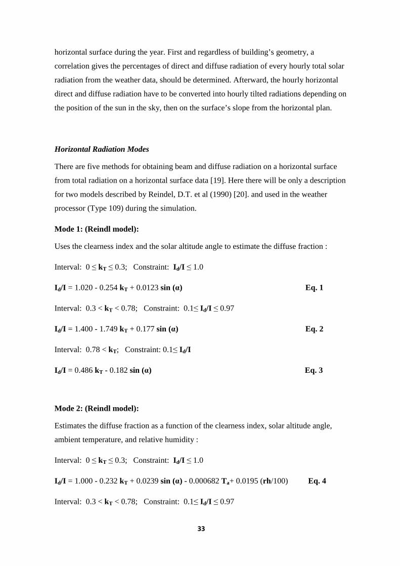
Horizontal Radiation Modes

There are five methods for obtaining beam and diffuse radiation on a horizontal surface

from total radiation on a horizontal surface data [19]. Here there will be only a description

for two models described by Reindel, D.T. et al (1990) [20]. and used in the weather

processor (Type 109) during the simulation.

Mode 1: (Reindl model):

Uses the clearness index and the solar altitude angle to estimate the diffuse fraction :

Interval: 0 ≤ kT ≤ 0.3; Constraint: I d/I ≤ 1.0

I d/I = 1.020 - 0.254 kT + 0.0123 sin (α) Eq. 1

Interval: 0.3 < kT < 0.78; Constraint: 0.1≤ I d/I ≤ 0.97

I d/I = 1.400 - 1.749 kT + 0.177 sin (α) Eq. 2

Interval: 0.78 < kT; Constraint: 0.1≤ I d/I

I d/I = 0.486 kT - 0.182 sin (α) Eq. 3

Mode 2: (Reindl model):

Estimates the diffuse fraction as a function of the clearness index, solar altitude angle,

ambient temperature, and relative humidity :

Interval: 0 ≤ kT ≤ 0.3; Constraint: I d/I ≤ 1.0

I d/I = 1.000 - 0.232 kT + 0.0239 sin (α) - 0.000682 Ta+ 0.0195 (rh /100) Eq. 4

Interval: 0.3 < kT < 0.78; Constraint: 0.1≤ I d/I ≤ 0.97

34

I d/I = 1.329 - 1.716 kT + 0.267 sin (α) - 0.00357 Ta+ 0.106 (rh /100) Eq. 5

Interval: 0.78 < kT; Constraint: 0.1≤ I d/I

I d/I = 0.426 kT + 0.256 sin (α) - 0.00349 Ta+ 0.0734 (rh /100) Eq. 6

For the above Horizontal Radiation Modes, beam radiation on Horizontal surface is

calculated by the difference between the total radiation and the diffuse component:

= − Eq. 7

Position of Sun in the Sky:

The position of the sun in the sky can be specified by giving the solar zenith and solar

azimuth angles. The zenith angle is the angle between the vertical and the line of sight of

the sun. This is 90 minus the angle between the sun and the horizontal (solar altitude

angle). The solar azimuth angle is the angle between the local meridian and the projection

of the line of sight of the sun onto the horizontal plane. Zero solar azimuth is facing the

equator, west is positive, while east is negative.

The zenith angle of the sun for each time step (here hourly) is given by the equation:

= + Eq. 8

Thus, the solar Azimuth angle is:

=

Eq. 9

TILTED SURFACE RADIATION MODE

There are four models for estimating the total radiation on a tilted surface. Each model

requires knowledge of total and diffuse (or beam) radiation on a horizontal surface as well

as the sun's position. The total tilted surface radiation is calculated by estimating and

adding beam, diffuse and reflected radiation components on the titled surface.

35

All titled surface radiation models use the same techniques for projecting the beam and

ground reflected radiation onto a tilted surface; they differ only in the estimate of diffuse

radiation on a tilted surface.

The contribution of beam radiation on a tilted surface can be calculated by using the

geometric factor Rb developed by Duffie, J. A. and Beckman, W.A. (1974) [21]:

=

Eq. 10

Where:

= + ( − ) Eq. 11

Once Rb is found,

= . Eq. 12

The contribution of reflected radiation on titled surface is calculated by assuming the

ground acts as an isotropic reflector, and defining Rr as the ratio of reflected radiation on a

titled surface to the total radiation on a horizontal surface is:

= . ( − ) ! Eq. 13

"!# = ". Eq. 14

The contribution of diffuse radiation on a tilted surface is determined by using one of four

models, isotropic sky model, Hay and Davies model, Reindel model, and Perez model.

Here the explanation will focus only on isotropic sky model, as it used mainly in this

study.

36

Isotropic sky model assumes that the diffuse radiation is uniformly distributed over the

complete sky dome. A factor Rd, the ratio of diffuse radiation on a titled surface to that on

horizontal, is given by :

$ = . ( + ) Eq. 15

Thus the diffuse radiation on a tilted surface assuming isotropic sky is:

= . Eq. 16

Thus the total radiation incident on a titled flat surface for all titled surface is given by the

equation:

= + + % Eq. 17

2.1.2 TRNBuild

Introduction

Type 56 models the thermal behavior of a building divided into different thermal zones. In

order to use this type, a separate pre-processing program must first be executed. The

TRNBuild program reads in and processes a file containing the building description and

generates two files (described later) that will be used by the TYPE 56 component during a

TRNSYS simulation.

This part describes the methodology been used to model reference building by using a

dynamic 3D building wizard of new version of TRNSYS.

A dynamic 3D-building simulation will carry out by TRNSYS using the 3D drawing

capabilities of Trnsys3d for Google Sketch-up, then importing the geometrical information

into the TYPE 56 (Multi-zone building model).

Type 56 needs a great amount of building data to calculate the thermal behaviour of the

building, these include geometry data, wall construction data, windows data,…etc. in

37

additional to weather data information such as: Radiation, ambient temperature,

humidity,…etc. furthermore, it needs information such as SCHEDUALE which may

define the gain from the occupants during the day with intervals representing the time

being occupant from the building owners.

To easily input the geometric information into the building model, a plug-in called

Trnsys3d for Goggle SketchUp™ has been developed. Trnsys3D Plug-in is not a full-

featured interface i.e. it will not help in creating non-geometry data, such as materials,

constructions, controls, internal heat gains, HVAC equipment and systems, etc..

Here a differentiation between Trnsys3d zones and SketchUp zones should be considered.

Trnsys3d zones must be convex i.e. every surface in the zone should be in the line of sight

with all other surfaces of the zone, since a Trnsys3d is designed to calculate the dynamic

energy flow for building, thus the energy model should be separated into perimeters and

zone core (thermal node) [22].

The Trnsys3d geometry which will be drown by SketchUp, will be written out on the

Trnsys3d file called: *.idf file which has all geometrical information about the modeled

building.

From 3D- Model to input files

Importing the *.IDF file

TRNSYS simulation studio offers the opportunity to automatically set up a simulation by

importing the *.idf file with the 3D-Building Wizard. After selecting the *.idf file from

the path which contain in the computer, a simulation with the important links for the first

run are automatically generated (Figure 12). A great advantage of the 3D-Building Wizard

is that all orientations of the Building are linked automatically. This reduces errors and

time used to link this information manually [23].

38

Figure 12. Multi-zone building model (Type 56) with all required connections

Due to the complexity of a multi-zone building, the parameters of TYPE 56 are not

defined directly in the TRNSYS input file, instead, a file so-called building file (*.BUI ) is

assigned containing the required information. TRNBuild has been developed to create the

*.BUI file which contains the basic project information, and user thermal zones

description (All information imported and defined)

During the importing of *.idf by 3D-Building Wizard in simulation studio, TRNBuild is

automatically run and doing the following steps:

• Sorting of zones/airnodes and surfaces

• Numbering of surfaces

• Volume calculation

• View factor to sky calculation

• Surfaces with the construction type “Virtual Surfaces” aren’t imported into

TRNbuild. (like Shading Objects)

• Generation of a *.BUI file and opening of the file in TRNbuild

39

• Generation of corresponding *_b17_IDF file with the same order of zones and

surfaces and the same surface numbers.

In TRNbuild non-geometric objects, such as materials, constructions, schedules, internal

heat gains, heating cooling etc. are added to the project, then the user can provide required

information to the project to have finally the desired outputs.

Generating files:

After creating the *.BUI file, which contains all required information about building,

TRNBuild uses it to generate standard TYPE 56 files and several other files (if detailed

Radiation modes are active). The standard files are automatically generated every time the

BUI file is saved, whereas the other files are generated by clicking on “Generate” button

of the main bar, in addition, the user always asked if the required files shall be generated

or not, before closing TRNBuild window [24].

1- Generating TYPE 56 standard Files:

As we already mentioned, the standard files are generated automatically, every time the

BUI file is saved which are:

• A file containing all information about the building excluding the wall construction

(*.BLD ) and

• A file contains the ASHRAE transfer functions for the walls (*.TRN ).

• In addition, an information file (*.INF ) is generated. This file contains the

processed (*.BUI ) file followed by the values of wall transfer function

coefficients, the overall heat transfer conductance U (KJ/hr.m2.k) and the related

U-value (W/m2.k). Next, the list of inputs required for the Type 56 is printed.

Also, the information file (*.INF ) provides a list of outputs of Type 56 as selected

by the user.

The (*.BLD ) and (*.TRN ) files are used by TYPE 56 during the simulation process.

40

2- Generating Shading / Insolation matrix

These matrices are generated as detailed beam solar radiation distribution mode in

“Radiation Mode” option active.

• SHading Matrix file called *.SHM .

• InSolation Matrix of a zone *_xxx.ISM . The triple X in the file's extension of

insolation matrix, later when the matrix generated for each zone, it will replace

with the zone’s number as it defined in TRNBuild.

For more detailed about the mathematical methods used to generate Insolation and

Shading matrices see Annex C

3- Generating view factor matrix *.VEM:

This matrix is generated, as detailed diffuse solar radiation mode and long wave radiation

exchange mode in “Radiation Mode” option active. (for more information see Annex C)

Lastly and before building simulation start to run, TRNBuild calling automatically to

create a file for the building description (*.BLD ) and another file for the transfer function

coefficients (*.TRN ) that characterize the wall constructions. These two files are

assigning internally to TYPE and include all information TYPE56 needs about the

building.

And if the detailed radiation modes were active, new matrices generating (*.SHM,

*_xxx.ISM, *.VFM ) and will be connected automatically by their names to TYPE

56.(Figure 13)

41

Figure 13. Input Files to Multi-Zone Building Model (Type 56)

Figure 14 is a flow diagram summarizing all previous steps to achieve a dynamic building

simulation using TRNSYS:

Figure 14. Flow diagram for a dynamic building simulation using TRNSYS

42

In Figure 14, the black dashed line heading from “Trnsys3d” to “TRNSYS Studio”

means that the generating of TRNSYS input files could be done either by importing the

(*.idf ) file via TRNBuild interface or via “3D Building Wizard” in Simulation Studio.

3.1.3 Mathematical Description of Type 56

The most important mathematical equations which Type 56 used to model the building are

summarized and presented in this section[25].

Thermal Zone /Airnode:

The building model in TYPE 56 is an energy balance model. The system boundary for this

energy balance includes the inside surface node of all surfaces of the zone. This balance

deals with radiative and convective heat flow into and out of the airnode.

Convective Heat Flux to the Air Node:

Figure 15. Convective Heat balance on the air node

Figure 15 shows the possible convective heat fluxes to the air node.

The convective heat balance is determined by the equation:

43

Eq. 18

Where:

convective heat gain from inner surface of zone (because of temperature

difference between airnode temperaure and surface temperature).

is the infiltration gains (air flow from outside only), given by

Eq. 19

is the ventilation gains (air flow from a user-defined source, like an HVAC

system, given by

Eq. 20

is the internal convective gains (by people, equipment, illumination, radiators, etc.)

is the gains due to (connective) air flow from airnode I or boundary condition,

given by

Eq. 21

44

Radiative Heat Flows (only) to the Walls and Windows:

Figure 16. Radiative energy flows considering one wall

Figure 16 shows the radiative heat fluxes to the airnode . This balance is determined by

the equation:

Eq. 22

Where:

is the radiative gains for the wall surface temperature node,

is the radiative airnode internal gains received by wall,

is the solar gains through zone windows received by walls,

is the long-wave radiation exchange between this wall and all other walls and

windows (εi =1)

is the user-specified heat flow to the wall or window surface.

45

Integration of Walls and Windows Figure 17 shows the heat fluxes and the temperatures that characterize the thermal

behavior of any wall or window.

Figure 17. Surface Heat Fluxes and Temperatures (Left) & and black box model of

the wall (Right)

The walls are modeled according to the transfer function relationships of Mitalas and

Arseneault [26,27,28] defined from surface to surface (from outer to inner surface), which

consider the wall as a black box(Figure 17). For any wall, the heat conduction at the

surfaces are:

Eq. 23

Eq. 24

These time series equations in terms of surface temperatures and heat fluxes are evaluated

at equal time intervals. The superscript k refers to the term in the time series, and it

specified by the user within the TRNBUILD description. The coefficients of the time

46

series (a's, b's, c's, and d's) are determined within the TRNBUILD program using the z-

transfer function routines of literature[27] .

A window is thermally considered as an external wall with no thermal mass, partially

transparent to solar, but opaque to long-wave internal gains.

In the energy balance calculation of the TYPE 56, the window is described as a 2-node

model shown in Figure 18. Eq. 23 is valid for a window with:

&' =

' = (' = $

' = )!,

&+ =

+ = (+ = $

+ = for k>0

Figure 18. Two-node window model used in th TYPE56 energy balance equation

The Long-Wave Radiation Standard model: Star network

For the star network approach a zone is restricted to a single airnode. The long-wave

radiation exchange between the surfaces within the airnode and the convective heat flux

from the inside surfaces to the airnode air are approximated using the star network [29]

and represented in Figure 19. This method uses an artificial temperature node (Tstar) to

consider the parallel energy flow from a wall surface by convection to the air node and by

radiation to other wall and window elements.

The thermal resistance between the artificial temperature node and temperature of the

airenode is given by:

47

,#-,. = /0&., -1/,.2 =

31/,.. (#,4& − #.) Eq. 25

Figure 19. Star network for a zone with three surfaces

The star temperature can be used to calculate a net radiative and convective heat flux from

the inside wall surface:

5('6,,.. = 5(,,.

. + 5,,.. Eq. 26

then:

5('6,,.. =

751.8,. -,.(#,. − #4&) Eq. 27

Where 5('6,,.. is the combined convective and radiative heat flux, and -,. is the

inside surface area.

48

According to the manual, the methods to calculate the resistances Requiv,i and Rstar,i can

be found in literature [29].

For external surfaces the long-wave radiation exchange at the outside surface is considered

explicitly using a fictive sky temperature, TSky, which is an input to the TYPE 56 model

and a view factor to the sky, fsky, for each external surface. The total heat transfer is given

as the sum of convective and radiative heat transfer:

5('6,,'. = 5(,,'

. + 5,,'. Eq. 28

Where:

5(,,'. = 9(':8,,'(#&, − #,') Eq. 29

5,,'. = ; <,'(#,'

= − #/+>= ) Eq. 30

#/+> = 0 − /+>2#&, + /+>#+> Eq. 31

Energy balances at the surfaces give:

5,.. = 5('6,,.

. + ,,. Eq. 32

5,'. = 5('6,,'

. + ,,' Eq. 33

Where:

Ss,I , Ss,o are the radiative heat flux absorbed at the inside and outside surface

respectively.

For internal surfaces Ss,i can include both solar radiative and generated long-wave

radiation (from persons or furniture).

For external surfaces, Ss,o consists of solar radiation only.

49

Detailed Model: Gebhart Method The detailed model for describing the heat exchange driven by long-wave radiation

exchange and convection. In detailed model, there is no artificial star node, since the long-

wave radiative heat transfer is treated separately.

Figure 20 shows the difference between the standard model and the detailed model.

Figure 20. Standard and detailed radiation model in comparison for a zone with three surfaces

The equations of detailed long-wave radiation heat transfer are based on the following

assumptions:

1. Absorption of radiation on a surface is indicated by a negative sign of the

corresponding heat flux, whereas net emission means a positive heat flux.

2. All surfaces are isothermal.

3. All surfaces are perfect opaque for long-wave radiation.

4. All surfaces are (diffuse) gray. i.e., the emissivity and absorptivity do depend neither

on wavelength nor on direction.

5. ρir is the hemispherical long-wave reflectivity

50

Detailed model uses the so-called Gebhart-Factor ?.,@→+ [30,31] is defined as the

fraction of the emission from surface Aj that reaches surface Ak and is absorbed.

?.,@→+ includes all the paths for reaching Ak, i.e. direct paths and one or multiple

reflection paths.

The abbreviation IR stands for “infrared”, meaning the long-wave range of the radiation

spectrum.

Using the assumptions from above the (dimensionless) Gebhart matrix for long-wave

radiation can be written as:

?. = (" − B .)CB. <. Eq. 34

where:

ρir and εir are diagonal matrices describing hemispherical long-wave reflectivity and

emissivity, respectively.

I variable describes the identity matrix.

F The view factor is defined as the fraction of diffusely radiated energy leaving surface

A that is incident on surface B.

Introducing the auxiliary matrix ?.∗ with dimension W/K 4 that given by:

?.∗ = 0" − ?.

# 2-. <. ; Eq. 35

Where:

?.# is the transpose of ?.

σ the Stefan–Boltzmann constant, and A the diagonal matrix describing the surface

areas.

?.∗ only depends on optical (emissivity, reflectivity) and geometrical (view factor, area)

properties as well as on the Stefan–Boltzmann constant.

Lastly, the net heat flux vector long-wave radiation in an enclosure is given by:

51

3.. = ?.

∗ #= Eq. 36

T ,is the temperature vector in the enclosure.

Optical and Thermal Window Model A detailed window model has been incorporated into the TYPE 56 component using

output data from the WINDOW 4.1 program developed by Lawrence Berkeley

Laboratory, USA [32]. This window model calculates transmission, reflection and

absorption of solar radiation in detail for windows with up to six panes. External and

internal shading devices and an edge correction for different glazing spacer types are

considered.

Description of window Figure 21 represents the window model in TRNSYS. This model may consist of up to six

individual glazing with fife different gas filling between them. Every window pane has its

own temperature node and the inner window pane is coupled via the star network to the

star node temperature of the building airnode. The outer window pane is coupled via

convective heat transfer to the temperature of the ambient air and via long-wave radiative

exchange with the fictive sky temperature, Tfsky .The heat capacity of the frame, the

window panes and the gas fillings are neglected.

For each glazing of the window, the resulting temperature is calculated considering

transmission, absorption and reflection of incoming direct and diffuse solar radiation,

diffuse short-wave radiation being reflected from the walls of the airnode or an internal

shading device, convective, conductive and long-wave radiative heat transfer between the

individual panes and with the inner and outer environment.

52

Figure 21. Detailed window model

Transmission of Solar Radiation Each glazing absorbs and reflects a part of the incoming solar radiation depending on

the glazing material and the incidence angle. In the program WINDOW 4.1, the detailed

calculation of reflection between the individual panes and the absorption and transmission

of each pane is performed hemispherically for diffuse radiation and in steps of 10°

incidence angle for direct solar radiation.

Together with the thermal properties of the gas fillings and the conductivity and

emissivity of the glazings, the optical data for the window is written to an ASCII file by

the WINDOW 4.1 program. This output file has a standard format, which makes the

results available for TRNSYS. (Figure 22)

This data is read by the TYPE 56 component and interpolated using the interpolation of

Akima /14/

Using this interpolated data, the transmission of solar radiation and the total absorption of

short-wave radiation for each window pane is calculated.

53

Figure 22. Window data used by the Type 56

Heat Flux between Window Panes

The heat transport between the individual window panes is shown in the Figure 23

below. Conduction, convection and long-wave radiation are considered separately.

Figure 23. Resistance network between window panes

The heat flux from the inner pane of the window to the ambient is calculated as:

54

3:C&. = ):C&. - . (#: − #&) Eq. 37

Where:

UUUUnnnn----aaaa is the overall heat transfer coefficient between inside and outside of window’s

panes

Absorption of Short-Wave Radiation The absorption of short-wave radiation (direct and diffuse solar radiation, diffuse reflected

radiation from the all the surfaces of the airnode and the optional inner shading device) on

the glazing system of the window leads to a heat flux from the pane to the airnode which

is given by:

3&,.. = ∑ (.→: ("$.&$.,. + "$./&$./,. + 0"7/, + "7/,92&$./,.,) .JK&

4'4) Eq.38

The total heat flux of such a glazing system can be split into a heat loss flux which is only

dependent on the temperature differences and the pane absorption heat flux which is only

dependent on the intensity of the short-wave radiation [33].

After having distributed all entering solar radiation for all airnodes of the building

including multiple reflections in an airnode or between airnodes via internal windows, the

calculations of surface temperatures and the window pane temperature calculations are

performed.

Total Energy Flux through the Window Glazing Having determined the individual pane temperatures and all of the heat fluxes through the

glazings, the absorbed short-wave radiation is summed over the various window panes and

distributed to the inner and outer window node. Based on the temperatures of the window

nodes, the absorbed short-wave radiation of the window nodes are found to be

3&,.. = . (3&

. + 9.(#. − #':7) − 9(,'(#' − #&6) − 3+>. ) Eq. 39

55

thus,

3&,&. = 3&

. − 3&,.. Eq. 40

Edge Correction and Window Frame

The calculations of the glazing temperatures of the window were performed for

undisturbed centre of glass values with no influence of the glazing edge. To take the cold

bridge effect of the spacer at the edge of the glazing system into account, edge correction

coefficients are calculated by the WINDOW 4.1 program for five different spacer

materials. The edge of the glazing is defined as an 2.5 inch (63.5 mm) wide area along the

perimeter of the glazing. These correction coefficients and the height and width of a

glazing sample defined in the TRNBUILD program and the U-value of the glazing is

calculated as a shunt circuit of centre of glass value, uuuucentrecentrecentrecentre and the U-value of the glazing

edge, uuuuedgeedgeedgeedge :

17$!7 = (7$!7, + (7$!7,S. 1(7:7 + (7$!7,T. 1(7:47S Eq.41

In the building description, the ratio of the frame area to the total window area (fframe) is

defined. Additionally a U-value for the frame is given there. The total U-value of the

window is calculated as the arithmetic mean value of glazing and frame U-value:

1U.:$'U = //&671/&67 + ( − //&67)1!V& Eq.42

The transmission of solar radiation is reduced by this fraction (to account for the opaque

frame part of the window). In the heat balance algorithm of TYPE 56, all the heat flows

and the resulting temperatures are related to the total window area.

56

Distribution of Solar Radiation through the window:

Direct radiation - standard model In standard direct radiation model, the incoming (primary) direct solar radiation is

distributed according to the distribution coefficients (GEOSURF) defined in the building

description. The sum of GEOSURF values given for all inside surfaces of a zone should

sum up to 1 at all times.

The fraction of incoming direct solar that is absorbed by any surface (i) is given by the

product of solar absorptance ααααssss value times the GEOSURF value given for this surface s.

If the GEOSURF values for all surfaces of a zone are set to zero, all direct solar radiation

entering this zone is treated as diffuse radiation and distributed with the absorptance-

weighted area ratios described below.

Direct radiation - detailed model For a detailed treatment of shortwave beam radiation shading and distribution, the multi-

zone building model reads in the sunlit factor matrices (Shading matrix (*.SHM ) and

Insolation matrices (*_xxx.ISM )) generated by TRNbuild at the beginning of the

simulation. For each time step the current sunlit fraction of surfaces are determined by a

bilinear interpolation of the four nearest center points with respect to the sun’s actual

position.

Diffuse radiation - standard model The incoming diffuse solar radiation and reflected primary direct solar radiation is

distributed according to absorptance-weighted area ratios. The fraction of diffuse solar that

is absorbed by any surface ssss is:

/$./,, = &-

∑(C $,)- Eq.43

57

Diffuse radiation - detailed model (Gebhart Method) The mathematical description of detailed diffuse model is similar to the long wave case,

but surfaces are assumed to be transparent. That means solar radiation enters the zone

from outside. The surfaces are not emitting radiation. They are assumed to be “passive”

because they are only reflecting, absorbing and/or transmitting solar radiation originating

from outside of the zone. Based on this idea, a (solar) Gebhart matrix can be created. For

opaque surfaces (walls) the transmitted diffuse solar radiation is zero.

The derivation of the describing equations for the detailed diffuse solar radiation heat

transfer is based on the following assumptions:

1- All surfaces are assumed to be transparent.

2- Radiation leaving a surface is indicated by a positive sign of the corresponding

heat flux.

Using the assumptions from above the (dimensionless) Gebhart matrix for diffuse solar

radiation can be written as:

?$./'V = (" − B $./'V)CB(" − $./'V) Eq.44

The abbreviation “difsol” stands for diffuse solar radiation.

Introducing the auxiliary matrix ?$./'V∗ with dimension m2 that given by:

?$./'V∗ = −?$./'V

# - Eq.45

?$./'V# is the transpose of ?$./'V and A is the diagonal matrix describing the surface

areas.

Thus, the net heat flux vector for diffuse solar radiation in an enclosure is given by:

3$./'V. = ?$./'V

∗ "$./'V Eq.46

3$./'V. is determined by a matrix multiplication with the driving force IIIIdifsoldifsoldifsoldifsol.

58

2.1.2 Mathematical description of Type 107

Single Effect Hot Water Fired Absorption Chiller: Single Effect Hot Water Fired Absorption Chiller Type107 [15] uses a normalized

catalogue data lookup approach (performance data) to model a single-effect hot-water

fired absorption chiller. Because the data files are normalized, the user may model any

size chiller using a given set of data files. However this type is not based on physical

phenomenon.

This type takes the required inputs from environment and then produces outputs which

also in turn connect with other types in the system. In addition, this type needs an external

data file (performance data) to work.(Figure 24)

Figure 24. Type 107 connections

Figure 25 demonstrates the performance data. These data contain values of normalized

fraction of full load capacity and fraction of design energy Input for various values of

fraction of design load (-) chilled water set point temperature (ºC) entering cooling water

temperature (ºC) and Inlet hot water temperature (ºC).

Figure 25. Absorption Chiller Performance Data of Type 107

Modeling of Type 107:

Type 107 is based on ordinary calculation and on external data (performance data) which

supply the required values: normalized fraction of full load capacity (The normalized

value of energy that is available to chill at current working conditions) and fraction of

design energy Input (the normalized value of heat input required to reach the va

fraction of nominal capacity). (Depended values) depend on fraction of design load (

chilled water set point temperature (ºC) entering cooling water temperature (ºC) and

hot water temperature (ºC). (Independent values).

Type107 first determines the fraction of design load at which it must operate first by

calculating the amount of energy that must be removed from the chilled water stream in

order to bring it from its entering temperature to the set point temperature:

The required energy removal is then divided by the machine’s capacity to determine the

fraction of design load at which the machine is required to operate:

Then Type 107 calls the dynamic data subroutine with the user specified chilled water set

point temperature, entering cooling water temperature, inlet hot water temperature, and

59

. Absorption Chiller Performance Data of Type 107




design energy Input (the normalized value of heat input required to reach the va

fraction of nominal capacity). (Depended values) depend on fraction of design load (

chilled water set point temperature (ºC) entering cooling water temperature (ºC) and

hot water temperature (ºC). (Independent values).

termines the fraction of design load at which it must operate first by




fraction of design load at which the machine is required to operate:


cooling water temperature, inlet hot water temperature, and

. Absorption Chiller Performance Data of Type 107




design energy Input (the normalized value of heat input required to reach the value for the

fraction of nominal capacity). (Depended values) depend on fraction of design load (-)

chilled water set point temperature (ºC) entering cooling water temperature (ºC) and inlet

termines the fraction of design load at which it must operate first by



Eq. 47


Eq. 48


cooling water temperature, inlet hot water temperature, and

60

fraction of design load and return the fraction of full load capacity and fraction of design

energy input for the specific values in the external data file at current work condition.

Afterward, type 107 calculates the machine capacity at the given time:

Eq. 49

When dynamic data returns the fraction of design energy input, then Type 107 calculates

the energy delivered to the chiller by the hot water stream:

Eq. 50

The hot water stream outlet temperature is then:

Eq. 51

The chilled water outlet temperature, which should be the set point temperature but may

be greater if the machine is capacity limited, is then calculated as:

Eq. 52

Now Type 107 can balance the energy in the machine by calculating the energy rejection

to the cooling water which given b the equation:

Eq. 53

Here term Qaux is counting for the energy needed auxiliary components on the entire

system and it used regardless if the machine works in a full capacity or not.

The temperature of the exiting cooling water stream can be calculated using equation:

Eq. 54

Finally, the machine COP is given by:

Eq. 55

61

Performance data description:

The performance data is an external manufacture data. Type 107 uses this data to predict

the machine performance. However, type 107 is not based on physical phenomenon,

which gives wide flexibility to different machines with different capacities to be tested and

validated.

Performance data consists of two basic group of variables (independent and depended

variables), and as already described, type 107 first calculates fraction of design load,

afterward, TRNSYS dynamic subroutine read the independent variables and then returns

depended variables at current working condition.

Figure 26. Example file for the performance data of the Absorption chiller

From the figure 26 right above it can be shown the followings:

The first four columns from the right are representing the independent variables which are

combined with the dependent variables on the left side of data. The change of the values

62

for the ‘fraction of nominal capacity’ only depend on the chilled water, the cooling water

and the hot water temperatures, the ‘fraction of design energy input’ further depends on

the value in the ‘Load’ column.

Fraction of design load determines the operation mode of the machine, when its value

equals 1, represents “full load” mode, and this represents its maximum value, and when its

value equals 0, represents “no load” mode, between those two values, “part load” mode is

represented.

For the values not directly within the range of independent variables, a linear interpolation

between the relevant data is carried out. An extrapolation beyond the range of the

independent variables is not possible. If a value beyond the limits of the data file is set,

always the last valid value of the data set is taken for the fraction of nominal capacity and

the fraction of design energy input.

P.S.: the Inlet Hot Water Temperature (IHWT) column of performance data (which

already existed in TRNSYS data library), was modified from old range (from 108.89 to

116.11 ºC) to another set of inlet temperatures (75 to 95 ºC), to comply with modelled

absorption machine (WEGRACAL SE 15) characteristics, since TYPE 107 unable to

execute an extrapolation beyond the range of the inlet temperature.

63

3.2 WUFIplus

Introduction:

WUFIplus is a room climate model which connects the energetic building simulation and

the hygrothermal component calculation. With the building simulation software

WUFIplus the hygric and thermal ratios in a building, in its perimeter and their interaction

can be calculated and quantified as well as the energy demand and consumption of system

engineering.

The simulation building can be modeled easy with aid of the Building Wizard. Numerous

assemblies and materials are already deposited in the accordant databases and can be

assigned to the components of the simulation building. [35]

Mathematical Model Description

Heat Balance:

Figure 27. heat flow into and out of thermal zone

64

Figure 27 shows the heat flow into and out of the thermal zone. These flows are balanced

as in this equation [36]:

. ( . ^. $_.$4 = 3('6`':7:4

. + 3U.:$'U. + 3"a3

. + 387:4. + 3b#

. Eq. 56

Where:

3('6`':7:4. heat exchange through opaque partitions.

3U.:$'U. heat exchange through windows.

3"a3. heat gain from people, equipment,…. etc.

387:4. heat flow ventilation (include natural and mechanical ventilation,

and infiltration).

3b#. heat flow from HVAC systems.

Heat Transport through walls:

Figure 28. Wall Heat transfer model

65

Heat exchanged through the opaque partitions of building envelope is given by

equation[36]:

3('6`':7:4 = ∑-. ). (#& − #.) Eq. 57

It should be noted that the overall heat transfer coefficient (U) will not have a constant

value during the simulation. Every time step, a new U-value will generate according to the

real values of surface and ambient temperature and other parameter depending on the

surface’s material.

Heat Transfer coefficients and resistances

If the wall or window surface warmer than the surrounding, heat starts to flow from them,

and this flow consists of three components: conduction, convection, and radiation (long

wave). Simplified model is used here since the detailed mode is so complicated it is not

necessary in the context of building physics, so simple model is usually adequate [37]:

5 = (∝(+∝). (#& − #) Eq. 58

Convective heat transfer coefficient:

The air adjacent to the component surface drains heat from the component by conductive

and convective heat transport. Although these are two distinct transport phenomena, they

are lumped together in the term of 'convective heat transfer'. Right close to the surface, air

layer has same wall temperature, in short distance away from wall surface, the temperature

has a constant distribution value. The convective between the surface and ambient

temperature is given by[37]:

5( = 9 . (#& − #,) Eq. 59

A detailed value of convective heat transfer coefficient, determined in a complex way

(Temp., air flow, wall types, ….etc.), but with free convection (by cooling or warming),

66

convective heat transfer coefficient in the range from 3 to 10 W/m²K, with forced

convection (by wind), in the range from 10 to 100 W/m²K.

Radiative heat transfer coefficient:

A wall surface always exchanges long-wave thermal radiation (wave length around 10

µm) with other surfaces in its surroundings. Since in most cases the temperatures of the

other surfaces are not known, they are assumed to be identical to the known air

temperature. This tends to low exchange of long wave radiation, and finally, net radiation

flows become so low. Equation describes long wave exchange contains two absolute

temperatures of two objects to power of four, but because of the relatively small

temperature differences, it can be linearized in good approximation. Then it given by[37]:

d = e&$ . (#,1'1:$.:! − #,) Eq. 60

For two close, extended, parallel, plane, non-metallic surfaces the r.h.t.c. lies between ca.

3 and 6 W/m²K.

Radiative heat transfer coefficient only applies to radiation exchange between surfaces

which are more or less at ambient temperature. Solar radiation (with a source temperature

of around 6000 k) is treated separately.

In compliance with recent changes in standardized terminology, WUFI now employs the

heat transfer resistance, which is simply the reciprocal of the heat transfer coefficient.

exterior heat transfer resistance:

0 m²K/W for basement walls in direct contact with the surrounding soil

0.04 m²K/W for floor and outer walls

interior heat transfer resistance:

0.13 m²K/W for basements, outer walls, roofs

67

Window modeling in WUFIplus:

Figure 29. Window model in WUFIplus

in WUFIplus net heat flux flows through the window computed in a simplified way,

taking into consideration transmission loss, because of the temperature difference between

inner zone temperature and ambient temperature.

Transmission loss (or gain) through window is given by equation[36]:

3# = -a. )a. (#& − #.) Eq. 61

Figure 30. Internal Distribution of short-wave radiation (Beam solar radiation)

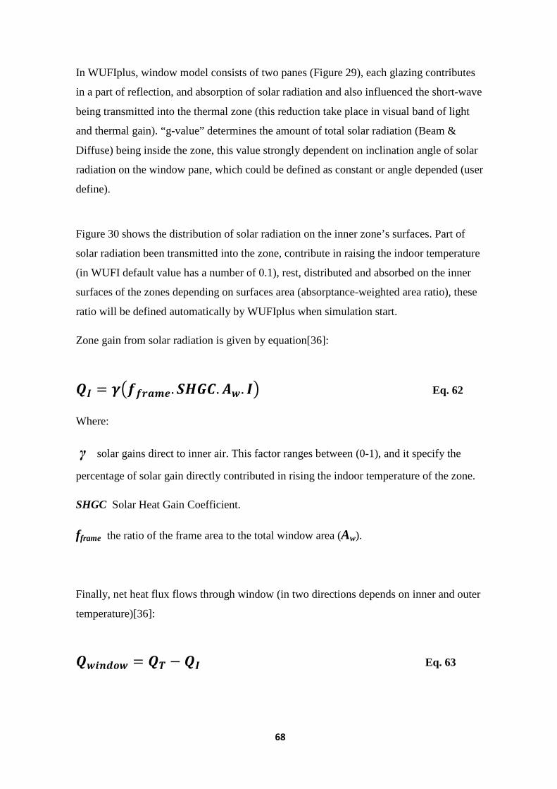
68

In WUFIplus, window model consists of two panes (Figure 29), each glazing contributes

in a part of reflection, and absorption of solar radiation and also influenced the short-wave

being transmitted into the thermal zone (this reduction take place in visual band of light

and thermal gain). “g-value” determines the amount of total solar radiation (Beam &

Diffuse) being inside the zone, this value strongly dependent on inclination angle of solar

radiation on the window pane, which could be defined as constant or angle depended (user

define).

Figure 30 shows the distribution of solar radiation on the inner zone’s surfaces. Part of

solar radiation been transmitted into the zone, contribute in raising the indoor temperature

(in WUFI default value has a number of 0.1), rest, distributed and absorbed on the inner

surfaces of the zones depending on surfaces area (absorptance-weighted area ratio), these

ratio will be defined automatically by WUFIplus when simulation start.

Zone gain from solar radiation is given by equation[36]:

3" = 0//&67. ,f?g. -U. "2 Eq. 62

Where:

γ solar gains direct to inner air. This factor ranges between (0-1), and it specify the

percentage of solar gain directly contributed in rising the indoor temperature of the zone.

SHGC Solar Heat Gain Coefficient.

fframe the ratio of the frame area to the total window area (Aw).

Finally, net heat flux flows through window (in two directions depends on inner and outer

temperature)[36]:

3U.:$'U = 3# − 3" Eq. 63

69

Radiation calculation in WUFIplus

Following the manual, WUFIplus converting the information provided for solar irradiation

into Direct and Diffuse components on tilted surfaces according to the following

methods.[38]

Direct radiation calculation on titled surface:

We assume that the input data are measured hourly values of the global IIIIGGGG and the diffuse

radiation IIIIdddd on a horizontal surface.

The direct radiation vertically incident on a surface which is facing the sun is the direct

normal radiation IIIIb,Nb,Nb,Nb,N. The direct radiation IIIIbbbb obliquely incident on a horizontal measuring

surface depends on the solar altitude:

" = ",k. & Eq. 64

Since IIIIbbbb can be determined as the difference between the measured values of global and

diffuse radiation and g can be determined from the measurement location and time by the

method given above, the corresponding direct normal radiation is:

",k = (" − "$)/ e Eq. 65

The direct radiation incident on the component surface is therefore:

"# = ":. = (" − "$). (' e Eq. 66

Diffuse radiation calculation

in WUFIplus, diffuse radiation treated as isotropic, and for non-horizontal surfaces, the

sky covers a smaller part of its field of view and the total amount of incident diffuse

radiation is reduced proportionately (a vertical wall sees sky only in the upper half of its

field of view):

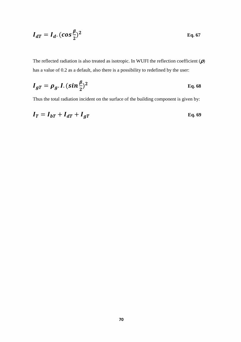
70

"$# = "$. ((' S)S Eq. 67

The reflected radiation is also treated as isotropic. In WUFI the reflection coefficient (ρρρρ)

has a value of 0.2 as a default, also there is a possibility to redefined by the user:

"!# = !. ". (.: S)S Eq. 68

Thus the total radiation incident on the surface of the building component is given by:

"# = "# + "$# + "!# Eq. 69

71

4. Building Simulation approach

4.1 Pre-analyze by WUFIPlus simulation

4.1.1 Analyzing solar gain of the new window design

In an attempt to clarify how the new window design of reference building react with solar

radiation; an investigation was carried out in WUFIplus. Two identical single-zone models

are created; however, each one has a design of external window different from each other.

One of these models has a usual or normal window design (Design A), while another one

has a prominent cuboid shape which represents the new window design of reference

building (Design B). (Figure 31)

The dimensions of the two single-zone models are taken arbitrarily (except windows area).

The net volume of each one was 50 m3. The glazings' area of “Design B” are taken same

as in the reference building, and equal to 0.88 m2 (Length=1.76 m, Width= 0.5 m) for each

one. The glazing's area of “Design A” is assumed to have an area of 1.25 m2 (Length=1.76

m, Width= 0.71 m)

Figure 31. Design B (left) and Design A (right) models

72

The glazing’s type which been used in the two designs is chosen the same, and has the

following properties: Low-e Double glazing, emissivity=0.2 , u-value=1.3, frame factor

=0.7, g-value (SHGC) has a range from 0.21 to 0.6 (incident angle depended), g-value

hemispherical (diffuse and long wave radiation)= 0.53.

Knowing that neither solar protection (Shading device), nor overhang has been applied in

this investigation.

Lastly, this simulation will take place at three orientations (South, North, and West), for

one year with time step equal to one hour. Weather data used in this work is taken from

TMY2 (Typical Metrological Year 2) and then converted to *.WAC (Weather Analysis

Center) format to be readable by WUFIplus.

4.1.2 Whole Building modelling

Introduction

Previous investigation about solar gain characteristics, may gave a picture of how solar

energy could be gained if such window shape is used. However, it’s not enough when the

aim is to know the influence on energy demand for a building which has more than one

window in different directions. Additional gain from these windows, and also the

influence of shading on each other may change the overall solar gain and hence the energy

demand of the building.

A simulation is carried out for whole building, and it has been decided to model it as a

“Single-Zone”, as the aim now in this step, is to define the overall solar gain, and to

optimize the direction of the building by testing different possible orientations.

The geometric dimensions used when the model built are as the following:

• Floor area to each floor equal to: 68 m2,

• height (two floor) equal to: 6.2 m,

• net volume of all building (after subtracting the thickness of walls and ceiling)

equal to: 312 m3.

73

The Building has been tested at the four main directions (North, South, West, and East),

afterward, solar gain and energy demand are determined and analyzed.

Modeling Approach:

WUFIplus has the advantages of creating a 3D-building’s model in the same environment

of the program (unlike TRNSYS) i.e. the user can create the structure, define the HVAC

systems and all boundary conditions of the building in the same area, which reduces the

time and effort to build such a model in comparison with TRNSYS method of modelling.

Creating the building model:

Here the steps of creating the model in WUFIplus work space (black background) are

skipped, as they are regarded simple and do not need to be explained, and the user can

figure out easily the way when uses the program for the first time.

Figure 32 shows the whole building model in WUFIplus from two different views.

Figure 32. Building model in WUFIplus

Building Structure(Walls, Roof, Ground):

Defining the structure of the model regarded the most important part of thermal building

analysis, since it determines the thermal behavior of the envelope and how the reaction

74

could be with the soundings (boundary condition) such as: ambient temperature, solar

radiation, long wave radiation, rain load …etc.

After creating the 3D model, the building structure now needs to be defined. The

definition of the wall, ceiling, floor and ground layers, can be easily done by using

“Material Database” existed in WUFIplus, which contains most of the materials used in

any building structure.

Simply, by selecting any part of the building model, which been already created on the

work space, then click “ASSEMPLY” button on the upper tap of the gray board,

afterward, then a new construction can be defined and built according to the real building

structure. (Figure 33)

Figure 33. Definition Wall’s Assembly (layers)

It should be noted that the most important property in this study is the U-value of the

structure (heat transfer coefficient). The walls and other building’s structure have built

taking into account only the required U-values as they defined from the owner of this

75

project (see Figure 1). Additionally, other properties such like absorptivity and emissivity

of the outer and inner surface of the wall should be considered.

The boundary condition of the “Ground structure” is exposed to air, i.e. there is a gap

between the lower ground structure and foundation. This boundary condition is possible to

thermally modeled in WUFIplus when there are adequate information about the

temperature of the soil during the year. The information have been taken from “Climate

Consultant” software and then defined in WUFIplus after setting the “Condition of outer

surface” as an “Optional Climate”.

Figure 34. Climate definition under ground floor construction

Figure 34 represents an example for Damascus. The temperature during the year takes a

“SIN” curve shape with average value equal 17 ºC occurred in June, with positive

amplitude of 7 ºC in September, and negative amplitude of 7 ºC in March.

Window Type:

Windows (glazing) are playing an incisive role in thermal building calculation. They

contribute in more energy loss and gain during the day and throughout the year than

building structure. This behaviour returns to its low thermal structural properties (thermal

inertia) comparing with heavy building structure (e.g. concrete).

The main task of the windows is to transmit visual light from the sun (visual band) to

reduce the bill of the lighting during the day when the sun shine, in addition, it can

76

transmit and absorb (depending on the wave length and the material) short wave radiation

(beam solar radiation), emit and absorb long wave radiation (emission which depends on

temperature difference between window’s pane and the surrounding), and it reflects small

part of incoming radiation.

Therefore, choosing the appropriate window type is a very important issue especially

when an efficient building aims to be designed. The most two important parameters

characterized the glazing are: g-vale (Solar heat gain coefficient) and u-value (heat

transfer coefficient of the window pane(s)).

In WUFIplus drawing a window (opening) something is not so complicated. First, the

structure which has to be opened should be selected, right click and then selecting

“OPENING” from the drop-down menu, then by inserting the window’s coordinates onto

the wall (i.e. width and length), WUFIplus create this opening. Kind of this opening either

“Transparent”(i.e. normal window) or just “Opening” (without any glass cover) should be

considered after the definition.

Hereafter, the definition of the window properties (thermal and optical) can be either from

external data, or from a “Database” are already existed in WUFIplus. The type which been

chosen in this study was: Low-e Double glazing, emissivity =0.2 , u-value=1.3, frame

factor =0.7, g-value (SHGC) has a range from 0.21 to 0.6 (incident angle depended), g-

value hemispherical (diffuse and long wave radiation)= 0.53. (Figure 35)

Figure 35. Definition Window (Glazing)

77

HVAC systems:

In WUFIplus, the definition of HVAC systems means: Heating, Cooling, Humidification,

Dehumidification, or Mechanical and Natural Ventilation.

The user can define one or more of those systems. Furthermore, the user can set the

capacity (power) of cooling or heating system, or determine the capacity (amount) desired

to remove or add in case of Humidification or Dehumidification respectively, or determine

the air change rate in case of Mechanical and Natural Ventilation.

In this study an investigation has carried out for Damascus and Abu Dhabi climates. In

Damascus, usually two systems are needed, cooling and heating systems. In Abu Dhabi,

usually there is only need for cooling system with dehumidification (heating system is

rarely required in such a climate).

For the ventilation, it has only applied “Natural” (window or door opening) to both cities.

Air exchange rate of “Natural” ventilation is taken from “MASDAR energy design guide

line “[39] as it regarded a proper code for efficient building design. The rate has entered 1

1/hr, and it set constant during the day and throughout the year. In addition, the value of

Leakage (infiltration) from windows and doors has been defined according to ASHRAE

90.1 standard [40]. The set-point temperature for cooling and heating are set according to

the Syrian Building Code [41] in case of Damascus, while in Abu Dhabi the set point

temperature was only for cooling system and it has been set according to “MASDAR

energy design guide line “[39]

Table 3 summarizing the properties of HVAC systems in Damascus and Abu Dhabi

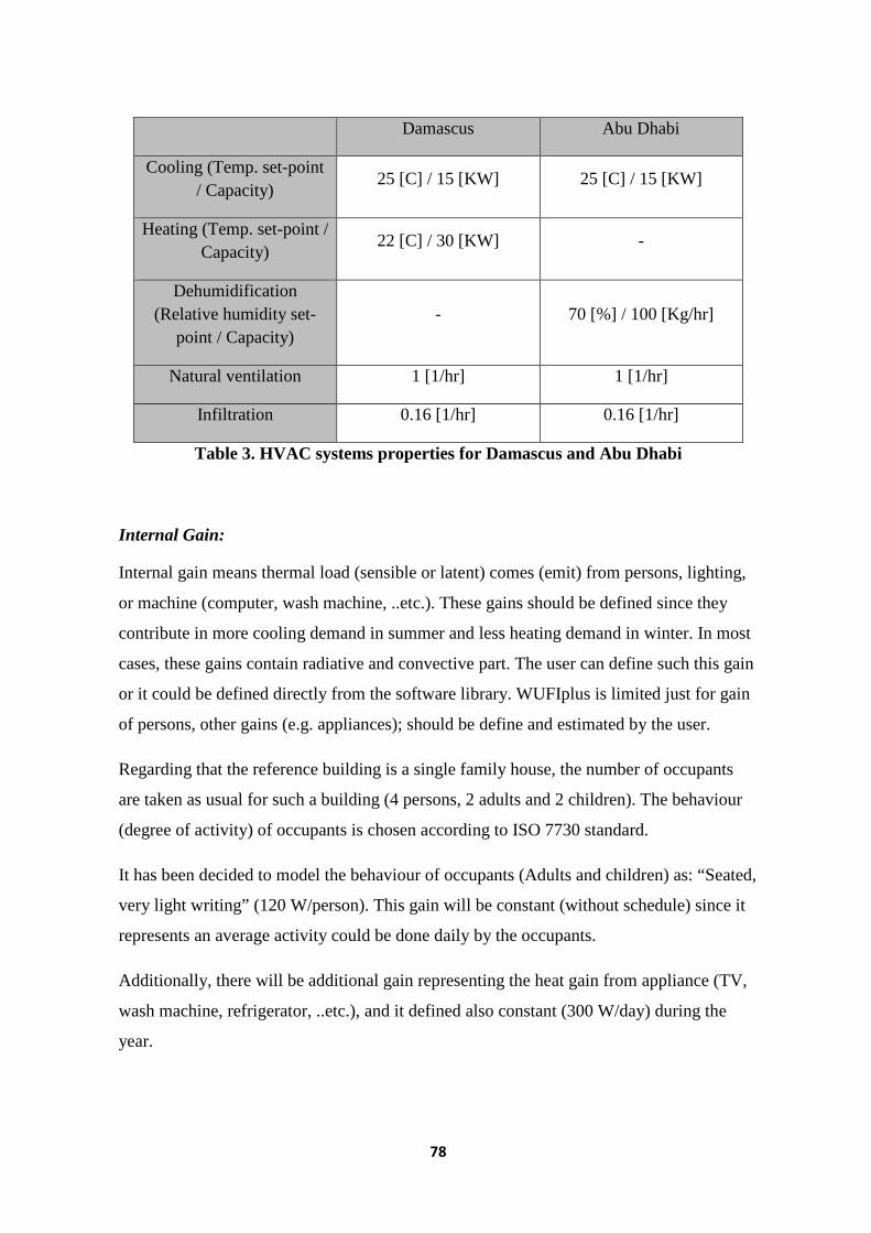
78

Table 3. HVAC systems properties for Damascus and Abu Dhabi

Internal Gain:

Internal gain means thermal load (sensible or latent) comes (emit) from persons, lighting,

or machine (computer, wash machine, ..etc.). These gains should be defined since they

contribute in more cooling demand in summer and less heating demand in winter. In most

cases, these gains contain radiative and convective part. The user can define such this gain

or it could be defined directly from the software library. WUFIplus is limited just for gain

of persons, other gains (e.g. appliances); should be define and estimated by the user.

Regarding that the reference building is a single family house, the number of occupants

are taken as usual for such a building (4 persons, 2 adults and 2 children). The behaviour

(degree of activity) of occupants is chosen according to ISO 7730 standard.

It has been decided to model the behaviour of occupants (Adults and children) as: “Seated,

very light writing” (120 W/person). This gain will be constant (without schedule) since it

represents an average activity could be done daily by the occupants.

Additionally, there will be additional gain representing the heat gain from appliance (TV,

wash machine, refrigerator, ..etc.), and it defined also constant (300 W/day) during the

year.

Damascus Abu Dhabi

Cooling (Temp. set-point / Capacity)

25 [C] / 15 [KW] 25 [C] / 15 [KW]

Heating (Temp. set-point / Capacity)

22 [C] / 30 [KW] -

Dehumidification (Relative humidity set-

point / Capacity) - 70 [%] / 100 [Kg/hr]

Natural ventilation 1 [1/hr] 1 [1/hr]

Infiltration 0.16 [1/hr] 0.16 [1/hr]

79

4.2 Modeling by TRNSYS

Now the modelling of the reference building will start in TRNSYS. Here there will be a

brief explanation about the building’s creating steps which had been done in Google

SketchUp™ to model the reference building. First, the main difference between this model

and WUFIplus model that the building is basically created as multi-zones building, and

this returns to the following reasons:

1- Since the reference building originally consists of two floors, it agreed to separate the

building into two main zones Ground and First floor (unalike in WUFIplus). These two

floors will be separated by an adjacent ceiling has a high insulation (according to the

project data). This separation will influence the distribution of solar radiation on the inner

zone’s surfaces, which in turns may influence the indoor temperature resulting in strong

effect on heating and cooling energy demand.

2- Due to programming issues in Google SketchUp™, it has been encountered a problem

in building the prominent windows shape of reference building connected directly with the

main two zones (Ground and First floor), because creating such configuration with edges

isn’t possible in this software. Hence, it agreed to separate these prominent part from the

main two zones, and define a new zone for each one of these windows, taking into account

the importance to define a “Coupling” between these zones and the main zones via the

adjacent openings.

4.2.1 Create a Trnsys3d Zone

Define the boundary for Trnsys3D zone:

After opening Google SketchUp™, we start to create a new Trnsys3d zone by choosing

Plug-in > Trnsys3d > New Zone Tool from the main menu. A small, blue cross-hair will

appear at the tip of the mouse pointer. Move over the axis origin until a small yellow dot

appears and click. This will place a blue box on the screen, which represents the Trnsys3d

zone border. Then double click on the axis origin should replace the blue outline of the

80

Trnsys3d zone into a slightly larger box with a broken, black outline. This ‘activates’ the

Trnsys3d zone. (Figure 36)

Figure 36. “Active” Trnsys 3D zone

After finishing the previous steps, starting to create Trnsys3D model now possible, make

sure that the Trnsys3d zone still ‘active’.

As already pointed out, it will be no detailed explanation about creating the geometry step

by step, only the important points will mentioned to be taken into account if similar work

may take place in the future.

Ground floor Trnsys3d zone:

This floor has an area equal to 70 m2 and its high equal to 3.1 m and its net volume equal

to about 212 m3. It should be note that the inner walls (adjacent walls) aren’t modeled

here, because of small floor area. Figures 37 below represents the final “Ground Floor”

zone with all fenestrations (Windows):

81

Figure 37. Ground floor Trnsys3d zone

From the Figure 37 right above, it can be noted two different adjacent’s: adjacent ceiling

to the first floor (Braun surface), and separated walls (highlighted red) contain glazings,

which represent the adjacent parts of ground floor to the window zones. These adjacent

windows will be defined as “Opening” in TRNBuild later, as it is in the reality.

First Floor Trnsys3d zone:

This floor has same characteristics of Ground Floor (area, height, volume). It should be

note that the inner walls (adjacent walls) aren’t modelled here, because of small floor area.

Figure 38 shows the first floor from two different view angles.

Figure 38. First Floor Trnsys3d zone

82

Windows Trnsys3d zones:

In this regard, and because of the difficulties which been encountered when trying to

create the main zones (First & Ground) as a one block, it agreed to model each window as

a single separated zone and then coupled it with main zone by defining a specific amount

of air flow between the main zone and windows zones through the adjacent glazings. All

window zones have been built with identical dimensions. (Figure 39)

Figure 39. Window Trnsys3d zone

Here when the Trnsys3d zones are created and placed together, then the construction

objects between “Ground” and “First” floor (adjacent ceiling), and between the windows

zones and the main two zones, should be defined as adjacent constructions. This usually

achieved either manually or automatically in Google Sketch-up.

Shading Objects:

Trnsys3d can be used to create shading objects, including overhangs and detached shading

objects to represent other buildings. In this project the shading group placed on the first

floor. Balcony and its hanged roof in the front side of building, they assumed as shading

objects which just contribute in calculation of the amount of solar radiation may blocked

83

to enter the building, but they will not computed or consider as walls or zones after

importing the *.idf file to TRNBuild. Figure 40 below shows the created shading objects.

Figure 40. Shading Objects

Lastly, after creating all previous zones, the final construction of building will look like as

in the Figure 41:

Figure 41. Multi-zone Building Trnsys3D model

84

4.2.2 Modelling of Reference Building by TRNSYS17

Figure 42. Zones of Building Model in TRNBuild

As already pointed out, the reference building has been modeled in TRNSYS as multi-

zone (unlike WUFIplus), two main zones representing the ground and first floor

(GROUND_FLOOR & FIRST_FLOOR), ten other zones representing the windows (e.g.

WINDOW5_F) which refer to the window number 5 and adjacent with First floor zone (F)

(see Figure 42). All these zones have same characteristics when we talk about Building

Structure, Windows type, Infiltration and Radiation Mode, but from the side of internal

gain, window zones are excluded.

Building structure:

The information about walls within a zone is displayed in the left lower part of the

AIRNODE window. Here, the user can add, delete or edit the walls of an AIRNODE. A

box in the upper part provides an overview of all defined walls. By clicking on a wall

within this overview box, the definition of the selected wall is displayed below and can be

edited.(Figure 43, left side)

85

Figure 43. First Floor Zone

Since the Building has been designed with a unique construction, i.e. high insulation,

therefore, the construction type of walls, ceiling, roof, and ground should be defined again

in TRNBuild, and ignoring the ready-made standard constructions according to ASHRAH

(American standard) or VDI 2078 (German standard), which are already exist in

TRNBuild library.

86

Figure 44. Wall Layers Definition

Here the wall layers from the program library can be selected. Creating the construction

started from the “inside” surface (front) of the wall to the “outside” (back). The building

structures are built according to the U-values that provided from the project owner (see

Figure 44)

The lower part of Figure 44 shows some important wall parameters: solar absorptance,

long wave emission coefficients and the convective heat transfer coefficient. These values

are left as default in TRNBuild.

To shorten the time need to define all zone walls, the user can select a previously defined

layer from the box in the left lower part of the AIRNODE window.

87

Windows type:

Windows can be defined for external and adjacent walls. If an external or adjacent wall is

selected in the overview box of walls, the right part of the AIRNODE window allows the

user to edit, delete or add windows for that particular wall. By clicking on a window

within the overview box, the definition of the selected window is displayed below and can

be edited.(see Figure 45)

The window type can be specified by using the pull-down menu on the right side. This

menu offers the options of defining a new window type, selecting a window type out of a

library or selecting a previously defined window type (see Figure 44 right side).

Figure 45. Windows Library

The criterion which followed to choose a proper window depended basically on U-value

and g-value of the glazing. A perfect thermal insulation (low u-value) and acceptable

value of solar energy gain (g-value) were the most important. Hence, the value of heat

transfer coefficient agreed to be in the range (1.3 ~ 1.4 W/m2.k), while g-value was in the

range of (o.5 ~ 0.65) in Damascus and Abu Dhabi. The German library is chosen, which

14 common window constructions of German glazing systems are available. The chosen

88

Window type was: WSV_AR_2. The properties of this type are presenting in the Figure

46 below:

Figure 46. (WSV2_AR_2) Window Type Properties

In this project, no internal shading is applied; just external shading will be addressed, to

see its influence on heating and cooling demand of the building and overall solar gain.

Coupling between airnodes of adjacent zones:

Since the project has already designed as multi-zone; airnodes with a specific amount of

air flow must be coupled. Coupling means that there is an air change between the

airenodes, due to pressure and temperature difference between them. This property

regarded important, as it influences the energy balance of building, because of its

contribution of sensible and latent heat energy gain or loss. (has the same effect of

ventilation but with lower amount as the temperature difference usually small between the

zones of same building).

The air flow rates had determined manually by monitoring the temperature difference

between the zones, and then try to minimize this difference as much as it can (i.e. with

reasonable values) by varying the air flow rates into and out from the zone.

89

Infiltration:

An air flow into the zone from outside the zone can be specified by INFILTRATION.

Here in TRNBuild, the Infiltration type involves: Natural ventilation (window opining)

and infiltration (air leakage from windows and doors).

Like in WUFIplus, the air change rate has specified according to “MASDAR energy

design guide line” [39], and it entered as a constant value during the day and throughout

the year. In addition, the value of Leakage (infiltration) has been defined according to

ASHRAE 90.1 standard [40]. Those two rates have summed-up, and then it entered as a

constant value into the infiltration type.

Damascus Abu Dhabi

Natural ventilation air exchange rate

1 (1/h) 1 (1/h)

Infiltration rate 0.16 (1/h) 0.16 (1/h)

Table 4. Natural ventilation and Infiltration rates of the reference building in case of Damascus and Abu Dhabi

Radiation Modes:

Direct and Diffuse short-wave radiation, Long-wave radiation exchange:

Detailed and standard modes have been used here

The necessity of using a detailed radiation modes because, in one hand, of the complexity

of window’s shape, and from another hand, the presence of adjacent openings which led to

more sophisticated solar radiation distribution going through these opening into the main

zone. Moreover, TRNSYS deals with the reflected short wave solar radiation -which is

basically beam radiation- as diffuse radiation, so a detailed calculation of diffuse radiation

distribution is also required here.

90

Internal Gains:

The behavior of occupants defined here like in WUFIplus (“Seated, very light writing”),

also it will take a constant value during the year, since it represents an average activity

could be done daily.

The chosen occupants behavior standard (ISO 7730) is already exists in TRNbuild library,

and just the scale (number of occupants) should be defined.

Additionally, there will be additional gain representing the heat gain from: Appliance (TV,

wash machine, refrigerator, ..etc.), and it defined constant (300 [W/day]) during the year.

Heating:

The heating requirement of any zone subject to idealized heating control can be

determined by specifying a heating type. Heating system could be modeled either by

define ventilation air change (here infiltration in our project), temperature and humidity as

inputs, fed by outputs from the conditioning equipment components, or the supplied

heating power should be defined as convective and radiative gain (Floor Heating or

Radiators).

In order to define a Heating type for the main two zones in this project, defining a NEW

heating type ( new system) should be done first - by clicking HEATING button in the

AIRNODE window - then; set point heating temperature heating, heating power, and

humidification set-point (according to relative or absolute humidity) have to be

determined. Knowing that the set-point heating temperature has set constant during the

day and throughout the year. Table 5

91

Damascus

Room Temperature Control

(set point) 22 ºC

Heating Power unlimited

Humidification -

Table 5. Heating system properties of the reference building in case of Damascus

It is worth mentioning that heating system has only been applied in Damascus, as Abu-

Dhabi has relatively no need for Heating. Set point temperature is taken from Syrian

Building Code [41].

Cooling:

The cooling requirement of any airnode subject to idealized cooling control can be

determined by specifying a cooling type. Same as pervious Heating System definition,

cooling system could be defined by ventilation, temperature and dehumidification, fed by

outputs from the conditioning equipment components, or via negative Convective and

Radiative system (Floor Cooling or Chilled Ceiling).

In order to define a cooling type for the main two zones in this project, defining a NEW

cooling type (new system) should be done first - by clicking COOLING button in the

AIRNODE window -, then the set point heating temperature cooling, heating power, and

dehumidification set-point (according to relative or absolute humidity) have to be

determined. Like in heating system, the set-point temperature cooling for Damascus and

Abu Dhabi have set constant during the day and throughout the year.

Table 6 summarizing the characteristics of cooling system in Damascus and Abu Dhabi

92

Damascus Abu-Dhabi

Room Temperature Control (set point)

25 ºC 25 ºC

Cooling Power Unlimited Unlimited

Dehumidification - 70 % (relative humidity)

Table 6. Cooling system properties of the reference building in case of Damascus and Abu Dhabi

Like in WUFIplus, all previous values are taken from Syrian Code [41] for Damascus,

while for Abu Dhabi they were taken from “MASDAR energy design guide line” [39].

93

5. Absorption Machine Modelling

5.1 Introduction

Refrigeration and air conditioning is used to cool products or a building environment. The

refrigeration or air conditioning system (R) transfers heat from a cooler low-energy

reservoir to a warmer high-energy reservoir (see Figure 47).

Figure 47. Schematic representation of refrigeration system

There are several heat transfer loops in a refrigeration system as shown in Figure 48.

Thermal energy moves from left to right as it is extracted from the space and expelled into

the outdoors through five loops of heat transfer:

Indoor air loop. In the left loop, indoor air is driven by the supply air fan through a

cooling coil, where it transfers its heat to chilled water. The cool air then cools the

building space.

Chilled water loop. Driven by the chilled water pump, water returns from the cooling

coil to the chiller’s evaporator to be re-cooled.

94

Refrigerant loop. Using a phase-change refrigerant, the chiller’s compressor pumps heat

from the chilled water to the condenser water.

Condenser water loop. Water absorbs heat from the chiller’s condenser, and the

condenser water pump sends it to the cooling tower.

Cooling tower loop. The cooling tower’s fan drives air across an open flow of the hot

condenser water, transferring the heat to the outdoors.

Figure 48. A typical Heat Transfer Loop in Refrigeration System

(Bureau of Energy Efficiency, 2004)

TYPES OF REFRIGERATION Systems:

Absorption Chiller

Absorption refrigeration systems are based on extensive development and experience in

the early years of the refrigeration industry, in particular for ice production. From the

beginning, its development has been linked to periods of high energy prices. Recently

however, there has been a great resurgence of interest in this technology not only because

of the rise in the energy prices but mainly due to the social and scientific awareness about

the environmental degradation.

Absorption systems are similar to vapour-compression air conditioning systems but differ

in the pressurisation stage. In general an absorbent, on the low-pressure side, absorbs an

evaporating refrigerant. The most usual combinations of fluids include lithium bromide-

95

water (LiBr-H2O) where water vapour is the refrigerant and ammonia-water (NH3-H2O)

systems where ammonia is the refrigerant.

Compared to an ordinary cooling cycle the basic idea of an absorption system is to avoid

compression work. This is done by using a suitable working pair. The working pair

consists of a refrigerant and a solution that can absorb the refrigerant. In the LiBr-H2O

system, water is the refrigerant. The system is shown schematically in Figure 49. The

pressurization is achieved by dissolving the refrigerant in the absorbent, in the absorber

section. Subsequently, the solution is pumped to a high pressure with an ordinary liquid

pump. The addition of heat in the generator is used to separate the low-boiling refrigerant

from the solution. In this way the refrigerant vapor is compressed without the need of

large amounts of mechanical energy that the vapor-compression air conditioning systems

demand. As shown in Fig.[], when the refrigerant vapor is coming from the evaporator

(10) it is absorbed in a liquid (1). This liquid is pumped to higher pressure (1-2), where the

refrigerant is boiled out of the solution by the addition of heat (3-7). Subsequently, the

refrigerant goes to the condenser (7-8) like in an ordinary cooling cycle. Finally, the liquid

with less refrigerant returns back to the absorber (6) [42]. The remainder of the system

consists of a condenser, expansion valve and evaporator, which function in a similar way

as in a vapour-compression air conditioning system.

96

Figure 49. Schematic of a single effect LiBr-water absorption system

.

The NH3-H2O system is more complicated than the LiBr-H2O system, since it needs a

rectifying column that assures that no water vapour enters the evaporator where it could

freeze. The NH3-H2O system requires generator temperatures in the range of 125°C to

170°C with air-cooled absorber and condenser and 80°C to 120°C when water-cooling is

used. These temperatures cannot be obtained with flat-plate collectors. The coefficient of

performance (COP), which is defined as the ratio of the cooling effect to the heat input, is

between 0.6 to 0.7. In the LiBr-H2O system water is used as a coolant in the absorber and

condenser and has a higher COP than the NH3-H2O systems. The COP of this system is

between 0.6 and 0.8 [43]. A disadvantage of the LiBr-H2O systems is that their evaporator

cannot operate at temperatures much below 5°C since the refrigerant is water vapour.

Commercially available absorption chillers for air conditioning applications usually

operate with a solution of lithium bromide in water and use steam or hot water as the heat

source. In the market two types of chillers are available, the single and the double effect.

The single effect absorption chiller is mainly used for building cooling loads, where

chilled water is required at 6-7°C. The COP will vary to a small extent with the heat

source and the cooling water temperatures. Single effect chillers can operate with hot

water temperature ranging from about 80°C to 150°C when water is pressurised [44].

97

The double effect absorption chiller has two stages of generation to separate the

refrigerant from the absorbent. Thus the temperature of the heat source needed to drive the

high-stage generator is essentially higher than that needed for the single-effect machine

and is in the range of 155 to 205°C. Double effect chillers have a higher COP of about

0.9-1.2 [45]. Although double effect chillers are more efficient than the single-effect

machines they are obviously more expensive to purchase. However, every individual

application must be considered on its merits since the resulting savings in capital cost of

the single-effect units can largely offset the extra capital cost of the double effect chiller.

Vapour Compression Refrigeration System

Compression refrigeration cycles take advantage of the fact that highly compressed fluids

at a certain temperature tend to get colder when they are allowed to expand. If the pressure

change is high enough, then the compressed gas will be hotter than our source of cooling

(outside air, for instance) and the expanded gas will be cooler than our desired cold

temperature. In this case, fluid is used to cool a low temperature environment and reject

the heat to a high temperature environment.

Vapor compression refrigeration cycles have two advantages. First, a large amount of

thermal energy is required to change a liquid to a vapour, and therefore a lot of heat can be

removed from the air-conditioned space. Second, the isothermal nature of the vaporization

allows extraction of heat without raising the temperature of the working fluid to the

temperature of whatever is being cooled. This means that the heat transfer rate remains

high, because the closer the working fluid temperature approaches that of the

surroundings, the lower the rate of heat transfer. The refrigeration cycle is shown in Figure

50 and can be broken down into the following stages:

1 – 2. Low-pressure liquid refrigerant in the evaporator absorbs heat from its

surroundings, usually air, water or some other process liquid. During this process it

changes its state from a liquid to a gas, and at the evaporator exit is slightly superheated.

2 – 3. The superheated vapour enters the compressor where its pressure is raised. The

temperature will also increase, because a proportion of the energy put into the

compression process is transferred to the refrigerant.

98

3 – 4. The high pressure superheated gas passes from the compressor into the condenser.

4 - 1 The high-pressure sub-cooled liquid passes through the expansion device, which both

reduces its pressure and controls the flow into the evaporator.

The condenser has to be capable of rejecting the combined heat inputs of the evaporator

and the compressor. In other words: (1 - 2) + (2 - 3) has to be the same as (3 - 4). There is

no heat loss or gain through the expansion device.[46]

Figure 50. Schematic of Vapor Compression Chiller System

CLOSED CYCLE ADSORPTION SYSTEMS

Instead of absorbing a liquid refrigerant with a solution, the refrigerant can also be

adsorbed to a highly porous solid. Different working pairs are suitable with these

adsorption systems: water/silica gel, water/zeloite, ammonia/activated carbon, etc[47].

Figure 51 shows a schematic of an adsorption chiller. The refrigerant, e.g. water, which

was previously absorbed in one chamber, is driven out of its porous solid using solar

energy. Using cooling water, the refrigerant is condensed at the top of the machine. Under

low pressure, the condensate is sprayed into the evaporator and evaporates again

producing the chilled water to drive the air-conditioning process. Afterwards, the vapor is

absorbed in the second chamber in a water cooled process. In order to guarantee a

continuous operation of the adsorption machine, the functions of the chambers are

changed after all refrigerant has been transported from one chamber to the other.

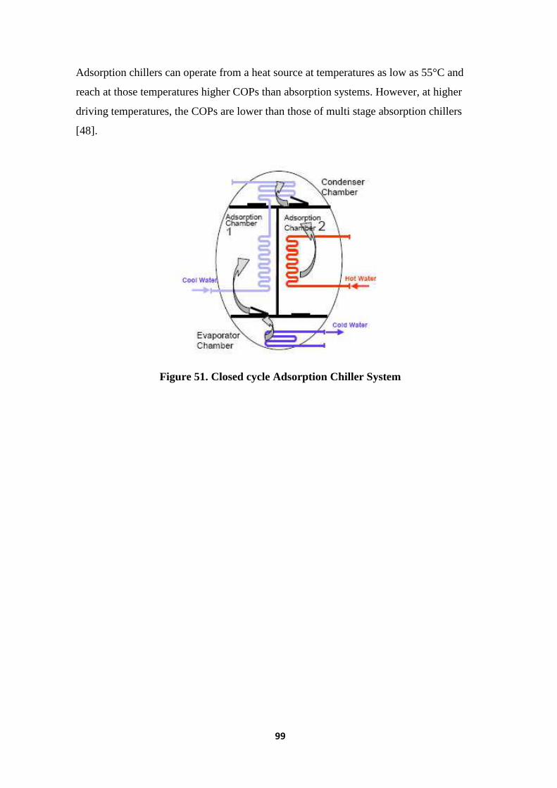
99

Adsorption chillers can operate from a heat source at temperatures as low as 55°C and

reach at those temperatures higher COPs than absorption systems. However, at higher

driving temperatures, the COPs are lower than those of multi stage absorption chillers

[48].

Figure 51. Closed cycle Adsorption Chiller System

100

5.2 Absorption Chiller modelling Method

5.2.1 Literature Review

Various computer simulation programs had been developed to predict the performance of

solar cooling systems in MENA countries.

Fathalah and Aly (1991) [49] in Jeddah, Saudi Arabia, a solar-powered combined system

comprising of a LiBr/H2O absorption chiller and a multiple-effect distillator had been

theoretically investigated. The absorption chiller is driven by tracking parabolic troughs

whereas the multiple-effect distillator was powered by the rejected heat from the

absorption machine. The overall COP of the system reached 1.44.

Ghaddar et al. (1997)[50] presented modelling and simulation of a solar absorption system

for Beirut. The results showed that for each ton of refrigeration it is required to have a

minimum collector area of 23.3 m2 with an optimum water storage capacity ranging from

1000 to 1500 l when the system is to operate only on solar energy for about 7 hours per

day. The economic analysis performed showed that the solar cooling system is slightly

competitive when it is combined with domestic water heating.

Hammad and Zurigat (1998)[51] described the performance of a 1.5-ton solar cooling

unit. The unit comprises a 14 m2 flat-plate solar collector system and five shell and tube

heat exchangers. The unit was tested in April and May in Jordan. The maximum value

obtained for actual coefficient of performance was 0.85.

In Iraq, Joudi and Abdul-Ghafour (2003) [52], have simulated a solar house cooling

system using different computer programs. The total effective collector area was 243 m2.

The LiBr/H2O absorption chiller used had a capacity of 35 kWc.

.

101

5.2.2 Absorption chiller system characteristics

This chapter focuses on the analyses of the energetic and economical performance of solar

powered absorption chiller system used to cover the previous investigated building. The

goals are to calculate the solar contribution to the total energy demand of the thermal

chiller system and to specify the associated costs.

The system was modeled with the TRNSYS simulation program. The simulation work is

based on hourly time series of irradiance and temperature data for Damascus / Syria. The

internal time step used was 1 hour. The hourly averages time series of both global

horizontal irradiance and temperature have been used a Typical Meteorological Year

version 2 (TMY2), which are available in the weather library of the TRNSYS simulation

environment.

The chilled water system for TRNSYS simulation is consisting of the following elements.

The system layout is given in Figure 52.

• Solar collector field

• Hot water buffer storage

• Absorption chiller (EAW (Wegracal SE 15)

• Wet cooling tower

• Cold water buffer storage

• External backup heater.

• Circulation pumps

102

Figure 52. Absorption Chillier system Configuration

The solar circuit are separated by a heat exchanger in hot storage tank. Hot water from the

hot water storage tank is feeding to the absorption chiller generator to provide cooling.

In case the cooling load cannot be met by solar means alone, an external backup

heater is foreseen for supplementary heating of the hot water loop to the generator.

Heat rejection is obtained by means of a wet cooling tower. For reasons of simulation

simplification the heat rejection unit, it assumed that in case of no adequate outlet cool

water temperature; a constant cooling water inlet temperature of 26°C to the absorption

chiller will be supplied. Also for reasons of simulation simplification, it has been assumed

that return temperature from cold distribution system of building always constant and

equal to the set-point temperature cooling minus three degree °C.

Building load was taken from the reference building in case of Damascus, oriented west,

without external or internal shading device, so that the chiller power of 15 kW nominal

cooling power of the German company EAW (Wegracal SE 15) is sufficient to maintain

room temperature levels at a given set point of 25°C for 100 % of all occupation hours.

Table 7 gives the technical data of the EAW WEGRACAL SE 15 Absorption Chiller.

103

Cooling power 15 KW Thermal COP

0.71

Cold water inlet 17 °C Cold water outlet 11 °C Cold water volume

flow rate 1.9 m³/hr

Nominal pressure loss

350 mbar

Nominal pressure 6 bar Cold water connection

DN 25

Heating power 21 KW Hot water supply 90 °C Hot water return 80.5 °C

Cold water volume flow rate

2 m³/hr Nominal pressure

loss 250 mbar


DN 25

Heat rejection power 35 KW Cooling water

supply 30 °C Cooling water return 36 °C

Cooling water volume flow rate

5 m³/hr

Nominal pressure loss

900 mbar


DN 32

Voltage / Frequency 400 V / 230 V

50 Hz

Electrical power consumption

0,3 kW

Length 1.5 m Width 0.75 m Height 1.6 m Weight 700 kg

Table 7. Technical Data of the EAW WEGRACAL SE 15 Absorption Chiller

Building load was calculated with a dominance of both: internal loads through persons and

equipment, and external loads through glazed facades (solar irradiance). The air exchange

rate was held constant at 1.16 (1/hr) for the building throughout the year, and it maintained

through natural ventilation. The type of cold distribution system in the building is assumed

to be: fan coils with 6°C / 12°C.

5.2.3 COMPONENT AND SYSTEM MODELS

TRNSYS program consists of many subroutines that model subsystem components. The

types which been used to model the cooling system are the followings:

104

• Single-effect Absorption Chiller (Hot water fired), the main model component. Its

Mathematical equations and internal calculation steps are described in detailed in

section (2.1.2)

• The construction and type of the solar collectors is important and relevant to the

operation and efficiency of the whole system. In this study, single-glazed Flat plate

collectors are considered modelled with TRNSYS Type 73. Type 73 models the

performance of a theoretical flat-plate collector. The Hottel-Whillier steady-state

model is used for evaluating the thermal performance.

• Hot water is stored in a TRNSYS Type 60 tank (Detailed fluid storage tank). Type

60 is a detailed model for stratified fluid storage tanks (multi-node).It includes

optional internal heat exchangers, which makes it suitable to our project model.

The storage tank has 10 temperature nodes to simulate stratification. The collector

injects heat into the storage tank via a internal heat exchanger. The return to the

collector is always taken from the bottom of the tank. The load supply is taken

from the top of the tank, while the load return is inserted into the tank bottom.

• Cold water storage is modeled in Type 4 (Stratified storage tank). The load supply

is taken from the bottom of the tank, while the return water from the distribution

system of building is always inserted into the top of the tank.

• The backup gas heater ( Type 6) is assumed to have a maximum heating rate of 18

kW and a set-point temperature of 95 ºC.

• A number of circulating pumps ( Type 3). Type 3 is a model for “single speed

pump” (constant flow rate), its ON and OFF function driven by control signals of

differential controller.

Figure 53 shows the final model of the absorption chiller in TRNSYS simulation

studio with all required Types and links.

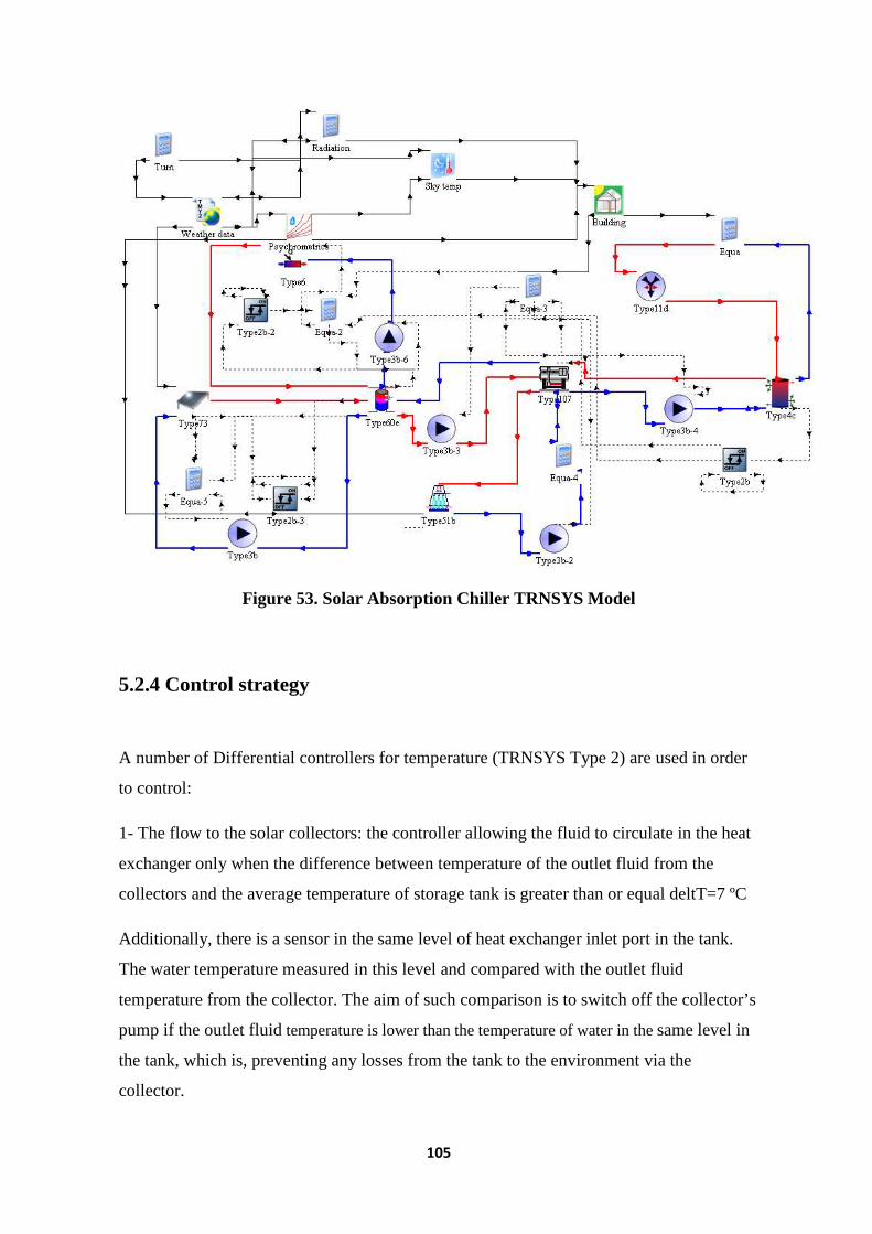
105

Figure 53. Solar Absorption Chiller TRNSYS Model

5.2.4 Control strategy

A number of Differential controllers for temperature (TRNSYS Type 2) are used in order

to control:

1- The flow to the solar collectors: the controller allowing the fluid to circulate in the heat

exchanger only when the difference between temperature of the outlet fluid from the

collectors and the average temperature of storage tank is greater than or equal deltT=7 ºC

Additionally, there is a sensor in the same level of heat exchanger inlet port in the tank.

The water temperature measured in this level and compared with the outlet fluid

temperature from the collector. The aim of such comparison is to switch off the collector’s

pump if the outlet fluid temperature is lower than the temperature of water in the same level in

the tank, which is, preventing any losses from the tank to the environment via the

collector.

106

2- The operation of gas heater: the controller allowing the gas heater to operate only when

the temperature of the fluid in the hot storage (the sensor assumed to be at node-2 near to

the tank’s top) below 80 ºC, in the same time the gas heater will prevent the temperature in

the tank to reach above 95 ºC (crystallization limit). In this case the heater will try to keep

the water temperature delivered to the absorption chiller always in the range of 80 ºC (in

sometime the inlet fluid temperature into the absorption chiller from the storage tank,

delivered lower than 80 ºC, since the back-up heater will be fired in the same time when

chiller run).

Knowing that the previous operation is taking into consideration the presence of cooling

demand from building, and control signal from absorption chiller operator. This logic is

implemented by equation:

OnOff_AHS = (OnOff_cold)*(OnOff_hot)*(OnOff_Qcool)

if OnOff_AHS > 0 P6 ON

if OnOff_AHS = 0 P6 OFF

Where:

OnOff_cold, is the control signal from the controller of absorption system.

OnOff_hot, is the control signal from the controller of back-up gas heater (operation of

gas heater).

OnOff_Qcool, is the control signal if there are cooling load from building or not.

This operation ensures effective firing of gas heater and less fuel consumption.

3- The operation of Absorption machine: here the controller allowing the three pumps

group (2, 3, 4) of absorption cycle to run as long as the temperature of the fluid in cold

storage above 17 ºC (the sensor assumed to be at node-6 of the tank). The controller

operates the chiller until the temperature of the fluid in the tank (in the same node level)

reaches 11 ºC.

Furthermore, the operation here needs verification from the building that there is a

demand before the system operate. This logic given by equation:

107

OnOff_System = (OnOff_Qcool)*(OnOff_AC)

if OnOff_System > 0 (P2 , P3 , P4) ON

if OnOff_System = 0 (P2 , P3 , P4) OFF

Where:

OnOff_AC , is the control signal from the controller of absorption chiller (operation of the

absorption machine).

In this situation OnOff_AC equal to OnOff_cold, as those two signals are output from the

same controller.

5.2.5 Performance Indicators

In order to evaluate the results of the simulation, the following energy related performance

criteria were defined [53]:

Net collector efficiency: The useful solar heat produced by the collectors QQQQcoll_usecoll_usecoll_usecoll_use

which is delivered to the thermally driven chiller, related to the radiation sum HHHHsolsolsolsol at the tilted collector aperture area:

ηnet = Qcoll_use / Hsol 0,... 1 or 0% - 100% Eq. 70

Specific collector yield: The useful solar heat produced by the collectors QQQQcoll_usecoll_usecoll_usecoll_use

used to drive the absorption chiller, related to the total collector area AAAAcollcollcollcoll:

Coll_yieldspec= Qcoll_use / Acoll kWh/m² Eq. 71

Solar fraction: The solar fraction quantifies the solar coverage on the total heat

requirements QQQQheat_totalheat_totalheat_totalheat_total

SF = Qcoll_use / Qheat_total 0,...1 or 0% - 100% Eq. 72

108

5.2.6 Primary energy consideration

The key parameter of energy related performance is primary energy saving by a solar

assisted system, due to the CO2 reduction. A very general analysis of the primary energy

consumption used in order to specify the optimum solar fraction when it compares with

the consumption of a conventional chiller

The analyzing done by using the following computation formulas [54]:

The specific primary consumption of a conventional chiller, driven by electricity,

sd,`,g':8 is given by the equation:

sd,`,g':8 = t7V7(4 .gus(':8

Eq. 73

For the absorption chiller, that uses a gas back-up heater as heat source when useful heat

from solar does not adequate to drive the chiller, the specific primary energy consumption,

is calculated using the equation:

sd,`,'V& = t/'.V . gus49

. ( − ,B) + sd`,(''V.:! 4'U7 Eq. 74

Thereby the specific primary energy consumption of the cooling tower is:

sd`,(''V.:! 4'U7 = d`,(''V.:! 4'U7t7V7(4

. ( + gus49

) Eq. 75

Where: Esp,cooling tower is: specific electricity demand of the cooling tower per unit of cooling energy

5.2.7 Pay Back Period

109

The main barrier of utilizing the absorption machine returns to its high initial cost, even

with low operation cost. On the other hand, the initial cost of conventional vapour

compression cooling system has low initial cost, but with high operating cost in

comparison with solar cooling system. The criteria has been used here to compare those

two system from economical point of view is: Pay Back Period (PBP) developed by

Duffie J, and Beckman W. (1991) [55], which is the time needed for the cumulative fuel

saving to equal the total initial investment:

svs =w ( g ./

d g/)

w(K./) Eq. 76

Where:

g = g,g. -,g + g,#. ^,# + g-g. 378&` + gg#. 3g# + g`16`. s`16` Eq. 77

d = ,B. 3!7: Eq. 78

Cs representing the initial cost of the whole component of absorption chiller, where, CSC,

CST, CAC , CCT, Cpump, are cost of solar collector, storage tanks, absorption chiller, and

pumps respectively.

Cf is the cost of fuel. if the inflation rate of fuel.

Es is he energy saving due to useful solar energy used.

5.2.8 Environmental Assessment and Global warming impact

Green House Gases (GHG) are the major cause for stratospheric ozone layer depletion.

Air conditioners and refrigerating machines are thought to this phenomenon. Examination

of the global warming impact of these machines requires consideration of both direct and

110

indirect effects. The direct impact relates to release of refrigerants (Hydroflorocarbons)

which regarded the most dangerous greenhouse gases on ozone layer, while the indirect

one refer to carbon dioxide production in electrifying the equipment or using fossil fuel.

The combined effect called “Total Equivalent Warming Impact” or (TEWI).

The direct component can be expressed in terms of an equivalent released amount of CO2,

as follows [56]:

x.7(4 (guS) = [z × k + dbb] . (9&!7 . ?as Eq. 79

Where:

MR: Make-up Rate: is the percent refrigerant charge lost per year

ELL: End Life Loss: is the percentage of refrigerant discharges out of the machine after

the service life.

N: Service life: is the number of years that the system is operational. [years]

R-charge: is the initial charge of refrigerant in the system [Kg]

GWP: Global Warming Potential: which is a ratio of how strong a greenhouse gas is (here

the refrigerant), compared to carbon dioxide.

The indirect effect from Absorption chiller is caused by using the back-up heater which

generates heat by burning natural gas. The indirect effect of AC is given by the equation:

":$.7(4(guS)'V = 3&1. <k? . k Eq. 80

Where:

Qgen: required heating energy to drive the absorption chiller during the year.

εNG: CO2 emission coefficient of natural gas

In the same time, using sub-solar thermal system will avoid the emission of CO2 into the

environment, since it reduces the consumption of fossil fuel to generate the required heat

111

to drive the absorption chiller . The amount of CO2 avoided by using solar absorption is

given by:

guS(-8'.$7$) = 3('VV_17/1V. <k?. k Eq. 81

The indirect effect is caused by the emission of CO2 from power plants used to generate

the electrical power needed to run the system and is:

For the conventional chiller:

":$.7(4(guS)(':8 = ~ 3(''Vgus(':8

. <7V7(4 . k Eq. 82

Where:

Qcool: overall cooling demand of building during the year

εelec: world average value of CO2 release for electric energy production.

6. Results and Discussion

6.1 Building Modeling

6.1.1 Simple model testing results

112

In this stage, two window designs were analyzed. The two model were tested under the

weather of Damascus. The term “Design A” refers to normal window design. The term

“Design B” refers to the prominent design of the windows of reference building (The

geometry and the characteristic of these two Designs were described in section 4.1.1).

Figure 54 shows the vertical view of “Design A” and “Design B” models which are used

for this simulation.

Figure 54. Design A (left) and Design B (rigth) Models

The main difference between those two designs that the two parallel glazings facades in

“Design B” always will be oriented 90 degree away from the specified orientation

(orientation of “Design A”).

The simulation results of the two models showed a strong relation between the sun’s paths

(see Annex B) and solar gain, furthermore, the results proved that there are big differences

in energy gained between the two designs at same orientation.

Figure 55 represents the situation of West orientation, and it can be noted that one of the

glazing in “Design B” faced North and the another one faced South.

Figure 55. Design A (left) and Design B (right) – West Orientation

113

Figure 56 represents the monthly solar energy gained at West direction for both designs.

Figure 56. Monthly Solar energy Gain Distribution – West Orientation

Figure 56 shows low solar gain in summer time in case of “Design B” in comparison with

“Design A”. This reduction in solar gain experienced by “Design B” returns to the

arrangement of the windows, which makes the sun always form high incident angles in

summer time, and because of short sun shine hours due to walls shading. While in winter

time, there is more gain collected in “Design B” than in “Design A”, due to low incident

angle (low sun altitude), and more sun shine hours on the southern glazing of “Design B”

than in “Design A”.

Taking the North orientation case. Here the two glazings of “Design B” oriented West and

East.(see Figure 57)

0

10

20

30

40

50

60

70

1 2 3 4 5 6 7 8 9 10 11 12

Sol

ar G

ain

(KW

h)

Time (month)

Design A

Design B

Figure 57. Design A (left

Figure 58 shows two peaks in fall and spring times from “Design B”, while “Design A”

shows one peak in the beginning of summer time (May). The solar gain profi

B” shows that in summer time

A”, and this return to more sun shine hours on both glazings of “Design B” (west and east)

during sunrise and sunset times than in “Design A”.

In winter time, most of solar gain

mainly from diffuse radiatio

wave radiation exchange with surroundings.

Figure 58. Monthly Solar energy Gai

0

5

10

15

20

25

30

35

40

45

50

1 2

Sol

ar G

ain

(KW

h)

114

Design A (left) and Design B (right) – North Orientation

shows two peaks in fall and spring times from “Design B”, while “Design A”

shows one peak in the beginning of summer time (May). The solar gain profi

me the collective solar gain has exceeded the one in “Design

nd this return to more sun shine hours on both glazings of “Design B” (west and east)

sunset times than in “Design A”.

solar gain in “Design B” and all of it in “Design A”

mainly from diffuse radiation (hemispherically and reflected beam radiation) and long

wave radiation exchange with surroundings.

Monthly Solar energy Gain Distribution – North Orientation

3 4 5 6 7 8 9 10 11 12

Time (month)

rientation

shows two peaks in fall and spring times from “Design B”, while “Design A”

shows one peak in the beginning of summer time (May). The solar gain profile of “Design

gain has exceeded the one in “Design

nd this return to more sun shine hours on both glazings of “Design B” (west and east)

B” and all of it in “Design A” will gained

and reflected beam radiation) and long

North Orientation

Design A

Design B

115

Figure 59 represents the case of South direction.

Figure 59. Design A (left) and Design B (right) – South Orientation

Figure 59 represents the case of South direction. Although the two glazings of “Design B”

here oriented toward west and east - like in North case -, but the response with solar

radiation was totally different, because the relative movement of the sun will keep the two

designs always projected to the sun during the day and throughout the year.

Figure 60. Monthly Solar energy Gain Distribution – South Orientation

Figure 60 proved that the continuous exposure to the solar radiation has reduced the

energy gained in summer in “Design A” and increased it in “Design B”, while the

situation in winter reversed markedly. Here the most influencing factor shaping these gain

0

10

20

30

40

50

60

70

1 2 3 4 5 6 7 8 9 10 11 12

Sol

ar G

ain

(KW

h)

Time (month)

Design A

Design B

116

profiles was the incident angle of the sun in regard with window pane, since in summer

time the incident angle formed small on the two glazings of “Design B” during the sunrise

and sunset, while in winter time, and because of small sun altitude angle, “Design A”

gained more due to small incident angle.

Discussion of the previous results:

Figure 61 shows a comparison of the gain profiles between “Design A” and “Design B” at

three different orientations.

Figure 61. Comparison between Design A and Design B at Different Orientations

This comparison shows convergence in solar energy gained during summer in case of

“Design B”, in contrast, it shows dissymmetry (spacing) when we talk about “Design A”.

In case of “Design A”, the simulation has proved that there is an extreme gain in summer

with 59 KWh in June and July at “West” direction, and very low solar gain in winter with

no more than 10 KWh in January at “North” direction.

Furthermore, the simulation has proved that the best situation, in respect with heating and

cooling demand criterion, was in “South direction in case of Design A” with very low gain

0

10

20

30

40

50

60

70

1 2 3 4 5 6 7 8 9 10 11 12

Sol

ar G

ain

(KW

h)

Time (month)

Design A /West

Design A /South

Design A /North

Design B /West

Design B /South

Design B /North

117

at summer (~ 27 KWh in June), and the highest solar gain ever at winter (~ 67 KWh in

Nov.) in comparison with “Design B” and other directions.

In case of “Design B”, the simulation has proved that the gain in summer time always

getting a range between 30 – 40 KWh/month, while in winter time the gains got wide

ranges but the upper limit did not exceed 47 KWh in March at North direction.

Finally, the overall results proved that in case of real building, mixing between two

designs may improve the thermal behaviour of building. In case of building has openings

on all facades, it could be possible to implement “Design A” at “South” direction, and

“Design B” in each of the remaining three directions (West, East, North). The comparison

showed the increment in solar gain in summer time in “Design B” in comparison with

“Design A” was not exceeded (30 %) in June, but in the same time, “Design B” can

collect more gain at other direction in winter time, in comparison with “Design A”.

6.1.2 Building Modeling results of WUFIplus

In this part, the simulation’s results of the reference building model will be presented.

According to the original shape of the reference building (see annex A), the model built

having two windows’ designs (Design A and B) distributed on all building’s facades (for

more detailed on the building’s geometry and dimensions see section 4.1.2).

The building has been simulated at four different orientations. The term “reference

façade” refers to the façade which is indicated in the Figure 62

118

Figure 62. Building Model in WUFIplus and the reference facade

Situation Damascus:

Figure 63 shows the two situations of reference building when reference façade either

oriented South or North.

In case of North orientation (on the left side), it can be noted three of “Design B” existed

at southern façade and two in northern façade. The other two facades only have normal

windows designs – like “Design A” - .

In case of South orientation (on the right side), the situation is totally opposite as it clear in

the Figure 63

It is obvious from Figure 63 that all glazings’ facades are facing either east or west

direction. Using sun’s paths graph of Damascus (see annex A). It is clear that “Design B”

and “Design A” will contribute in more solar gain in summer time (longer sunshine hours

during sunrise and sunset). In winter time, solar radiation will always hit the windows in

high incident angles, i.e. low solar gain in winter (low g-value).

Attention should be paid on the effect of self-shading. “Design B” are positioned close to

each other and this may prevent more possible gain especially in summer time.

Figure 63. Building Position in Case of North (left) and South (right) Orientation

119

Figure 64 shows the two situations of whole building when reference façade either

oriented West or East.

It is obvious from Figure 64 that all glazings’ facades are facing either North or South

direction. It is clear that “Design B” and “Design A” will contribute in more solar gain in

winter time (low incident angles). In summer time, solar radiations will always forming

high incident angles with the windows, i.e. low solar gain in winter (low g-value).

Figure 64. Building Position in case of West (left) and East (right) Orientation

0

200

400

600

800

1000

1200

1400

1 2 3 4 5 6 7 8 9 10 11 12

So

lar

Ga

in (K

Wh)

Time (month)

West

East

North

South

120

Figure 65. Monthly Solar Energy Gain Distribution (from left to right: West, East, North, South) / Damascus

Figure 65 represents the monthly solar gain distribution of the whole building at four

different orientations, and it shows the followings:

• The highest solar gain ever has achieved in summer time in case of “South”

orientation.

• In summer time, there is a considerable difference in solar gain between “North or

South” case, and “West or East” case. This difference, in its extreme situation, was

around 86 % in June.

• In case of “West” and “East” orientations, there was an increment in solar gain in

winter time than in “North” and “South” orientation.

• In winter time, there is a slight increase in solar gain in case of “East” orientation

than in “West” orientation. This increment due to that the main façade (see figure

5) in the case of East orientation was oriented towards south (more solar gain).

While in case of “West” orientation, the “main facade” was oriented toward north

(low solar gain).

• In December, there is low solar gain at all orientations. This return to possible

clouds in the sky, and the gain will only come from diffuse radiation and long

wave radiation exchange.

Figure 6 shows that the lowest collective solar gain from the sun was at West (~ 8231.6

KWh/year). The highest solar gain was at North (~ 10644 KWh/year).

121

Figure 66. Annual Solar Energy Gain at Four Different Orientations / Damascus

All previous investigation about solar gain led to parallel conclusion of the energy demand

for building. The simulation proved that when there is much solar gain, the demand for

heating will be less, while cooling will be higher.

Figure 67 presents cooling and heating demand of all four directions.

Figure 67. Annual Heating and Cooling Energy Demand at Four Different Orientations / Damascus

From the Figure 67 it can note the followings:

0

2000

4000

6000

8000

10000

12000

West East North South

So

lar

Ga

in (K

Wh)

0

1000

2000

3000

4000

5000

6000

7000

8000


Ene

rgy

Dem

and

(KW

h)

Cooling

Heating

122

• The highest cooling energy demand achieved when the reference façade oriented

“South” with 6907 KWh/ annually.

• The lowest cooling energy demand achieved when the reference façade oriented

“West” with 5280 KWh/ annually.

• The highest heating energy demand achieved when the reference façade oriented

“South” with 6597 KWh/ annually.

• The lowest heating demand achieved when the reference façade oriented “East”

with 6200 KWh/annually.

Figure 67 shows (relatively) equal annual heating demand for all orientations, and the

difference did not exceed 7 % in its extreme situation (South and East). In the same time,

the results shows a significant difference in overall cooling demand between (“North” or

“South”) and (“West” or “East”). This difference reached in its extreme situation (North

and West) around 31 %.

Finally, it could be concluded that the best orientation in regard with energy demand was

at “East” orientation. Furthermore, “West” orientation could be also another best case, as

the difference with “East” was relatively very low and it can be ignored.

Situation Abu Dhabi

Figure 68 represents the sun-paths diagram of Abu Dhabi.

123

Figure 68. Sun Paths (Abu Dhabi)

It can be noted from Figure 68 the shifting of sun paths slightly towards the top of the

diagram in comparison with Damascus. This shifting means more sunshine hours in winter

time in Abu Dhabi than Damascus. However, the length of the day in summer time

became less than in Damascus. These changed in paths return to the low latitude of Abu

Dhabi.

Since in Abu Dhabi the same steps have been followed in testing the optimum orientation,

here it will only present the results and its potential reasons.

Figure 69 presents the monthly solar gain for four orientations.

124

Figure 69. Monthly Solar Energy Gain Distribution (from left to right: West, East, North, South) / Abu Dhabi

Figure 69 shows some similarities in solar gain distribution like in Damascus (but with

different amplitudes). That is because most of sun paths are in common for the two cities.

The distribution of gain for West and East orientations were homogenous during the year.

(unlike Damascus). The monthly average value of solar gain was around 800

KWh/monthly for East, and around 770 KWh/monthly for West case.

Regarding North and South orientations. The gain distribution looked to be the same in

Damascus but with less energy in summer time and higher in winter time.

Taking the summer time, the high sun altitude angle (low g-value) and shorter days led to

lower gain in comparison with Damascus. In winter time, the building gained more

energy, that’s because of long day hours i.e. more sunshine hours, even with relatively

high sun altitude.

The yearly value of solar gain showed that the largest gain was achieved in case of South

direction, while the lowest gain was achieved in case of West direction (see Figure 70).

0

200

400

600

800

1000

1200

1 2 3 4 5 6 7 8 9 10 11 12

So

lar

Ga

in (K

Wh)

Time (month)

West

East

North

South

125

Figure 70. Annual Solar Energy Gain at Four Different Orientations / Abu Dhabi

Figure 70 showed that the largest solar gain was achieved in case of “South” direction.

However, this huge amount of solar gain was not reflected on high cooling energy demand

at “South” orientation. A monthly-based solar gain comparison (see Figure 69)showed the

following: at “South” orientation, there is more solar gain in summer time and lower in

winter time in comparison with “North” orientation. This difference led to higher cooling

demand in “South” orientation than “North” orientation and not the opposite.

Knowing that the lowest cooling demand was achieved in West case, where the demand

not exceeded 18574 KWh/annually.(see Figure 71)

Figure 71. Annual Cooling Energy Demand at Four Different Orientations / Abu Dhabi

8000

8500

9000

9500

10000

10500

11000


So

lar

Ga

in (K

Wh)

17800

18000

18200

18400

18600

18800

19000

19200

19400

19600

19800

20000


Ene

rgy

De

ma

nd (K

Wh)

126

Furthermore, the cooling system in Abu Dhabi is assigned with dehumidification system.

The yearly demand was around 2353 KWh/annually. Knowing that the energy need for

dehumidification will be always the same for any orientation, as the amount of air change

rate is always the same as well.

Building modelling results with external shading

In order to optimize the passive measures of the building, an external shading device is

applied.

The shading factor has been estimated according to the picture of reference building. In

WUFIplus, the definition of shading factor (solar protection in WUFI) is: the ratio of

window area covered by shading to window area without shading. For this study, shading

factor it has been inserted 0.3 [-] for Damascus and Abu Dhabi, which means, 70 % of

window area will be covered by shading.

The mechanism of shading system depends on a control strategy. This control measures

the indoor temperature of the zone, and returns back a logic value either one or zero.

These values translated in shading system as “shading” or “no shading” respectively. This

mechanism is preventing an excessive indoor heating by solar radiation in summer time,

in the same time, it allows solar radiation entering the zone in winter time (Passive

heating). Figure 72 shows the shading factor and the chosen operation mode (controlling

mode)

Figure 72. External Shading Device Definition in WUFIplus

127

Building simulation in case of Damascus showed a considerable reduction in solar gain

and cooling demand. Figure 73 shows that the solar gain reduction concentrated in

summer time when this gain is not needed. In winter time, control system of shading

device did not reduce the solar gain to cover some of heating loads.

Figure 73. Monthly Solar Energy Gain With and Without External Shading Device / Damascus-West

The overall reduction in solar gain during the year reached about 43 %. This reduction

translated to parallel reduction in cooling demand to become around 3318 KWh/annually

instead of 6559 KWh/annually in case of “no-shading”. This means less cooling energy

demand by 60 [%].(see Figure 74)

0

100

200

300

400

500

600

700

800

900

1 2 3 4 5 6 7 8 9 10 11 12

So

lar

Ga

in (K

Wh)

Time (month)

Without Shading

With Shading

0

200

400

600

800

1000

1200

1400

1600

1 2 3 4 5 6 7 8 9 10 11 12

Ene

rgy

De

ma

nd (K

Wh)

Time (month)

Without Shading

With Shading

128

Figure 74. Monthly Cooling Energy Demand With and Without External Shading Device / Damascus-West

Figure 75 represents the monthly solar energy gain distribution in Abu Dhabi /West with

and without shading. It is obvious that the reduction in solar gain occurred throughout the

year. In another word, this investigation proved that solar radiation always has a negative

role and always leads to more cooling demand in this region.

Figure 75. Monthly Solar Energy Gain with and Without External Shading Device / Abu Dhabi-West

The overall reduction in solar energy gained during the year reached about 170 %. This

reduction translated to parallel reduction in cooling energy demand. The new yearly

cooling demand became around 13897 KWh/annually, instead of 18574 KWh/annually in

case of “no-shading”. This is mean less energy consumption by 33.6 %. (see Figure 76)

0

100

200

300

400

500

600

700

800

900

1000

1 2 3 4 5 6 7 8 9 10 11 12

So

lar

Ga

in (K

Wh)

Time (month)

Without Shading

With Shading

129

Figure 76. Monthly Cooling Energy Demand With and Without External Shading Device / Damascus-West

In case of Abu Dhabi, the results proved that the strong reduction of solar gain in Abu

Dhabi (170 %) is not translated to huge reduction in cooling demand (33.6 %). While in

case of Damascus, the image was the opposite, i.e. a moderate reduction in solar gain

(47%) offset by huge reduction in cooling energy demand (60 %). These differences

return to the followings:

1- Longer cooling season in Abu Dhabi (from March to the end of Nov.) in

comparison with Damascus (May to the mid of Oct.).

2- Longer sunshine hours in Abu Dhabi than in Damascus in winter time. While in

summer time, Damascus has longer sunshine hours but with lower sun altitude

angles than in Abu Dhabi (more heat received per square meter) .

3- Higher average ambient temperature at night in Abu Dhabi than in Damascus, i.e.

more energy to cooling down the indoor temperature.

Additionally, In Abu Dhabi, there is more energy consumption from the dehumidification

system in summer time.

Those entire factors are translated to more energy needs for cooling in Abu Dhabi than in

Damascus.

0

500

1000

1500

2000

2500

3000

3500

1 2 3 4 5 6 7 8 9 10 11 12

Ene

rgy

De

ma

nd (K

Wh)

Time (month)

Without Shading

With Shading

130

6.1.3 Building Modelling Results of TRNSYS

The aim from TRNSYS modeling is to validate the results of WUFIplus and see where

is the deviations and its potential reasons.

WUFIplus simulation showed that the best orientation in case of Damascus and Abu

Dhabi was at “West”. Hence, the TRNSYS 3D model of the reference building has

been built in Google Sketch-up oriented “West” as well. The radiation distribution

modes (Beam, diffuse, and long-wave radiation) have been chosen as “Detailed”, and

no external or internal shading has been applied.

Figure 77 demonstrates the monthly distribution of solar gain in Damascus-West. Like

WUFIplus, TRNSYS results show less solar gain achieved in summer time than in

winter time. The annual average solar gain around 530 KWh/annually throughout the

year.

Figure 77. Monthly Solar Energy Gain Distribution / Damascus-West

Regarding the energy demand, TRNSYS simulation for Damascus found to be have an

energy need for heating equal to 14462 KWh/annually, while the cooling demand was

around 2496 KWh/annually. (see Figure78)

0

100

200

300

400

500

600

700

1 2 3 4 5 6 7 8 9 10 11 12

So

lar

Ga

in (K

Wh)

Time (month)

131

Figure 78. Monthly Heating and Cooling Demand Distribution / Damascus-West

An investigation was carried out for the yearly average airnode floating temperature

(airnode temperature without heating or cooling system). This investigation was only

for First and Ground floor zones (main zones). The results showed that the yearly

average floating temperature of those two zones was around ~18.5 ºC. The

investigation’s results explains the reason of enormous amount of heating energy

demand (set-point heating is 22 degree C) and low cooling demand (set-point cooling

is 25 degree C) in the building.

Applying an external shading device on all external windows of building model

showed a reduction in solar gain. The shading factor is taken same like in WUFIplus

which assumed that external shading device covers 70 % of glazing. It should be noted

that the definition of shading factor in TRNSYS different from WUFIplus. In

TRNSYS software, the shading factor is defined as: the ratio of non-transparent area

of shading device to the whole glazing area, which means value of 1 refers to zero

transmission, thus, 70 % corresponded to a factor of (0.7). This factor is inserted as

constant and it only applied from mid of May to the mid of Oct. (cooling season)

Figure 79 shows the definition of external shading device in TRNBuild.

-1000

-500

0

500

1000

1500

2000

2500

3000

3500

1 2 3 4 5 6 7 8 9 10 11 12

Ene

rgy

De

ma

nd (K

Wh)

Time (month)

Haeting

Cooling

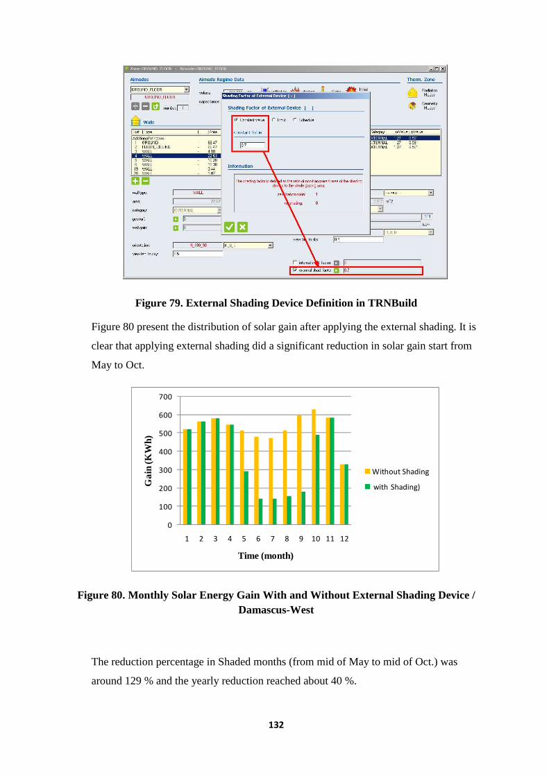
132

Figure 79. External Shading Device Definition in TRNBuild

Figure 80 present the distribution of solar gain after applying the external shading. It is

clear that applying external shading did a significant reduction in solar gain start from

May to Oct.

Figure 80. Monthly Solar Energy Gain With and Without External Shading Device / Damascus-West

The reduction percentage in Shaded months (from mid of May to mid of Oct.) was

around 129 % and the yearly reduction reached about 40 %.

0

100

200

300

400

500

600

700

1 2 3 4 5 6 7 8 9 10 11 12

Ga

in (K

Wh)

Time (month)

Without Shading

with Shading)

133

It is obvious that the shading process will contribute in reducing the cooling demand.

The resultant cooling demand when shading applied was around 1132 KWh/annually,

and this means yearly reduction by 120 %. (see Figure 81)

Figure 81. Monthly Cooling Demand Distribution With and Without External Shading Device / Damascus-West

The last Figure 81 shows disappearance of cooling demand in May and September, and it

only limited to three months during the year.

6.1.4 Modeling results validation (WUFIplus vs. TRNSYS)

A comparison between WUFIplus and TRNSYS results of the whole building was

carried out. The compared results are taken from the previous simulation results of

Damascus / West.

The initial findings of this comparison found huge differences in case of energy

demand and solar gain. Regarding heating energy demand, the annual difference

reached 120 % more in TRNSYS, while the annual cooling demand difference reached

around 112 % more in WUFIplus.

0

100

200

300

400

500

600

700

800

1 2 3 4 5 6 7 8 9 10 11 12

Ene

rgy

De

ma

nd (K

Wh)

Time (month)

Without Shading

With Shading

134

Figure 82 shows the monthly deference in heating and cooling demand between

WUFIplus and TRNSYS

Figure 82. Monthly Cooling and Heating Demand Comparison between WUFIplus and TRNSYS / Damascus-West

Regarding solar gain, the results showed different monthly amplitudes, and annual

increment was around 30 % more in WUFIplus.(see Figure 83)

The mismatching in solar gain, returns to the different way that the two tools uses to

distribute the solar radiation inside the zones. WUFIplus software uses “absorptance-

weighted area” method to distribute the solar radiation on the inner surfaces. TRNSYS

17 in case if “Detailed” mode was chosen, the distribution of solar radiation is not

constant (unlike WUFIplus) and may in some time concentrates in one or two surfaces

inside the zone, while the other surfaces just receive reflected direct or diffuse

radiation. Additionally there will be a portion of direct solar radiation goes out through

other external windows in the zone. (see mathematical description for more detailed).

These differences in distribute solar radiation regarded incisive factors led to increase

the gain in WUFIplus than in TRNSYS.

-2000

-1500

-1000

-500

0

500

1000

1500

2000

2500

3000

3500

1 2 3 4 5 6 7 8 9 10 11 12

Ene

rgy

De

ma

nd (K

Wh)

Time (month)

Cooling /TRNSYS_Detailed

Cooling /WUFI_ShCal

Heating /TRNSYS_Detailed

Heating /WUFI_ShCal

135

Figure 83. Monthly Solar Energy Gain Comparison between WUFIplus (Shading Calculation active) and TRNSYS (Detailed Radiation Mode) / Damascus-West

Concerning the previous differences, an initial comparison focused on solar gain is

carried out between those two tools.

In TRNSYS, “Standard” and “Detailed” radiation distribution modes have been used.

In WUFIplus, the “Shading calculation” on external windows from walls or other

object was activated then deactivated.

Table 8 summarizes the results of this investigation. Here the percentages are representing

the annual difference of collective solar gain between the investigated modes.

Solar gain WUFIplus (shading calculation from all

assemblies is deactivate)

WUFIplus (shading calculation from all assemblies is active)

TRNSYS (Standard Radiation Mode)

3 % for WUFIplus 10 % for TRNSYS

TRNSYS (Detailed Radiation Mode)

50 % for WUFIplus 30 % for WUFIplus

Table 8. Solar Gain Comparison results between WUFIplus and TRNSYS

The investigation results showed that in case of “Standard” radiation mode in TRNSYS,

and when the “Shading calculation” in WUFIplus set deactivate, the annual collective

0

100

200

300

400

500

600

700

800

900

1 2 3 4 5 6 7 8 9 10 11 12

So

lar

Ga

in (K

Wh)

Time (month)

TRNSYS_Detalied

WUFI_ShCal

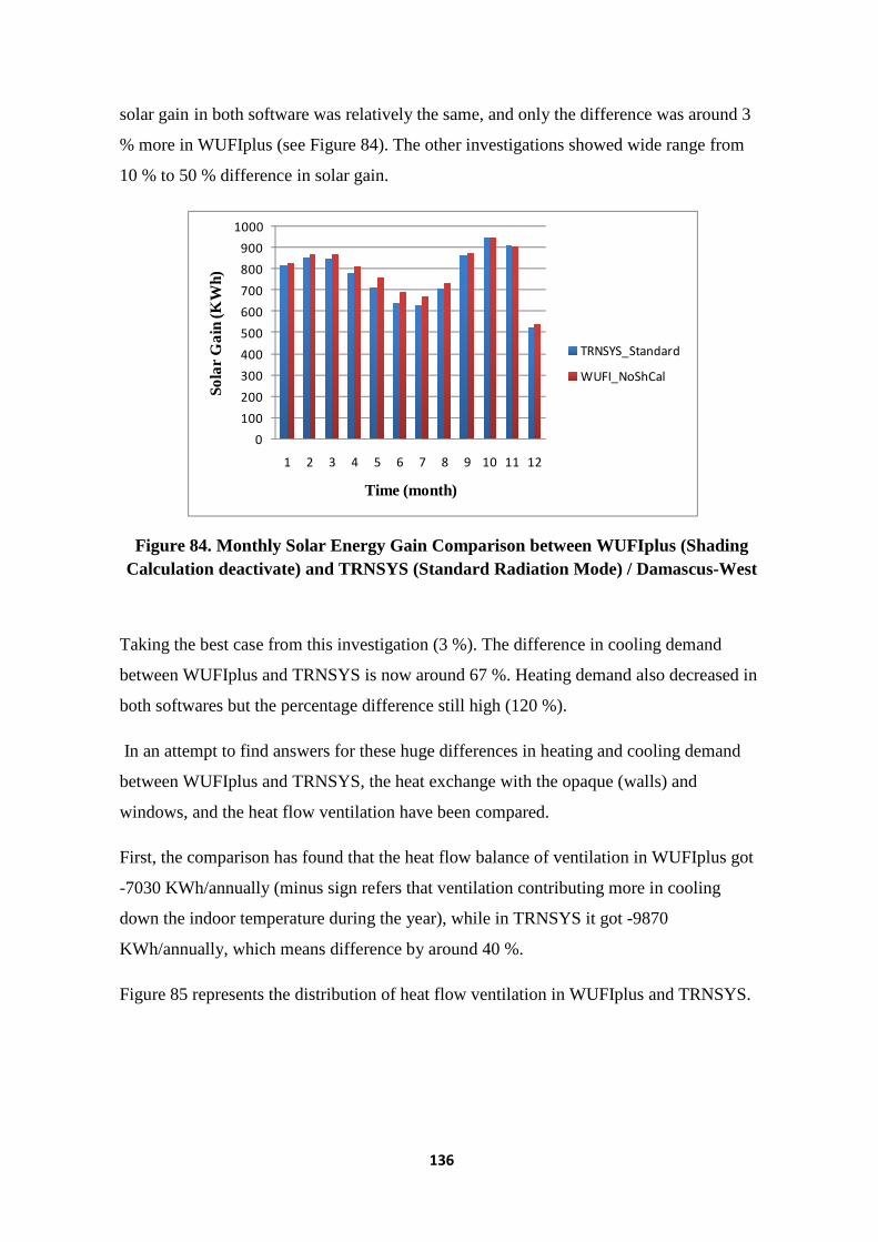
136

solar gain in both software was relatively the same, and only the difference was around 3

% more in WUFIplus (see Figure 84). The other investigations showed wide range from

10 % to 50 % difference in solar gain.

Figure 84. Monthly Solar Energy Gain Comparison between WUFIplus (Shading Calculation deactivate) and TRNSYS (Standard Radiation Mode) / Damascus-West

Taking the best case from this investigation (3 %). The difference in cooling demand

between WUFIplus and TRNSYS is now around 67 %. Heating demand also decreased in

both softwares but the percentage difference still high (120 %).

In an attempt to find answers for these huge differences in heating and cooling demand

between WUFIplus and TRNSYS, the heat exchange with the opaque (walls) and

windows, and the heat flow ventilation have been compared.

First, the comparison has found that the heat flow balance of ventilation in WUFIplus got

-7030 KWh/annually (minus sign refers that ventilation contributing more in cooling

down the indoor temperature during the year), while in TRNSYS it got -9870

KWh/annually, which means difference by around 40 %.

Figure 85 represents the distribution of heat flow ventilation in WUFIplus and TRNSYS.

0

100

200

300

400

500

600

700

800

900

1000

1 2 3 4 5 6 7 8 9 10 11 12

So

lar

Ga

in (K

Wh)

Time (month)

TRNSYS_Standard

WUFI_NoShCal

137

Figure 85. Monthly Heat Flow Ventilation Comparison between WUFIplus and TRNSYS / Damascus

Knowing that the air change rate inserted identical for the two softwares (1 1/hr), and also

they used a weather data from the same source (TMY2). Further investigation about the

volume that been used in ventilation calculation shown a difference. In WUFIplus, wall

layers is constructed from “Outside” to “Inside”, i.e. the thickness of the wall will cut part

of building’s volume. In TRNBuild, the situation is opposite, i.e. it constructs the layers

from “Inside” to “Outside”.

To make sure if the last situation contributed in heat flow ventilation difference, the

volume has manually modified in WUFIplus and inserted the same volume as in

TRNBuild. The results showed a consistency in heat flow ventilation and the yearly

difference was not exceeded 2.2 % more in TRNSYS. This small difference may occur

because of applying the zones’ coupling in TRNBuild. The coupling influences the

convective heat flow between the coupled zones, as it calculates the heat flow resultant

because of temperature difference between the zones (see mathematical description).

-2500

-2000

-1500

-1000

-500

0

500

1 2 3 4 5 6 7 8 9 10 11 12

He

at F

low

(KW

h)

Time (month)

TRNSYS

WUFI

138

Figure 86. Annual Net Heat Flow Ventilation before and after Building’s Volume Change

Finally, changing the building’s volume reduced the difference in energy demand of

building between WUFIplus and TRNSYS. In case of cooling demand, the difference after

the changing got around 69% more in WUFIplus, instead of 67% before changing, which

means no much changes was happend. While the results of heating demand found a

considerable reduction, and the difference now got around ~ 68 % more in TRNSYS,

instead of 120% before the change taking place.

Regarding the case of heat exchange through the opaque partitions and windows, in

WUFIplus the results found around +3050 KWh heat exchanged annually through the

building envelope (positive sign refers that heat exchange contributing more in heating up

the zone during the year). In TRNSYS, the heat exchange balance got very huge losses

(more of the heat are flowing to the outside), and it was around -13650 KWh/annually.

An investigation for internal radiative and convective heat transfer resistances for walls

and windows are carried out. The simulation has found some differences in the way of

calculation of those two resistances. In WUFIplus, the calculation of overall heat transfer

coefficient (U-value) always depends on a constant value (either as default or user

defined) of internal and external combined (radiative and convective) heat transfer

resistances. In TRNBuild, the calculation of internal and external combined heat transfer

resistances depending on “long-wave radiation” mode used. In case of “Standard”

0

2000

4000

6000

8000

10000

12000

Net

he

at f

low

(KW

h)Heat flow

ventilation(TRNSYS)

Heat flow ventilation

(WUFI_Before)

Heat flow ventilation

(WUFI_after)

139

radiation mode -which been used here-, the net long-wave radiation exchange between

surfaces and airnode (indoor air) done by applying the so called: “Equivalent heat transfer

resistance” between the inner surfaces and “artificial temperature node” (Tstar),

furthermore it uses another resistance (Star resistance) for the heat convective exchange

with the temperature of airnode (see mathematical description of Type 56 for more

detailed). Searching has been done to find the source and values of radiative and

convective resistances which been used in above mentioned resistances (Equivalent and

Star). The results found that there is only a possibility to adapt the convective part of

combined resistance, whereas the radiative part is calculated internally in TRNBuild

during the simulation, and the user cannot define or change it manually.

Lastly, these differences in combined resistances’ calculation between WUFIplus and

TRNSYS, maybe influenced the final results, and created the previous deviations in

overall heat exchange rates between WUFIplus and TRNBuild. In turn theses problem led

to the differences in estimating the energy demand of the building model.

6.2 Absorption Chiller Modeling results:

The case study considered in this work corresponded to solar absorption refrigeration

system serving a demand for air conditioning for building under the climate of city of

Damascus.

The size and properties of the Absorption chiller (EAW Wegracal SE 15) has been

adapted to comply with the cooling demand of building. Testing for the highest cooling

capacity in building found 3.2 KW (~ 1 TR) for all zones, hence, the origin Pumps’ flow

rates have been reduced by factor of (4.7).

The performance of the system is affected by various factors. These factors are the

collector tilt angle, the mass flow rate through the collectors, the storage tank volume and

the collector area. A number of simulation runs were carried out in order to investigate

these factors’ effects on the system performance, but only the factor of “collector area” is

140

analyzed numerically, by comparing the primary energy consumption of the system in

comparison with conventional Vapor Compression Chiller (VCC).

The influence of solar collector area on the solar fraction of the solar system is shown in

Figure 87, in which it is observed that an increase in the collector area increases the value

of annual solar fraction, an effect that also increases if in the simulation is considered a

collector with higher efficiency.

Figure 87. Solar Fraction

The results of varying the collector area on the useful collector energy and the required

auxiliary heating energy to drive the chiller can be seen in Fig. 88.

Figure 88. Useful Collector Heat vs. Heat from Back-up

60

65

70

75

80

85

90

95

100

6 8 10 12 14 16

Collector Area (m2)

0

200

400

600

800

1000

1200

1400

6 8 10 12 14 16

Use

ful H

eat (

KW

h)

Collector Area (m2)

Qaux

Qcoll_useful

141

Figure 88 showed an inversely proportional between useful energy gained from solar and

energy supplied from back-up heater to drive the chiller. The purpose of the solar sub-

system is to ensure that most of the absorption cycle required heat is provided by the

collectors. In addition, the selected collector area has to result into lower energy

consumption than that of a vapor-compression cycle (VCC) if it used instead of solar

absorption chiller.

The following assumption factors have been used to calculate the primary energy

consumption in both solar absorption chiller and conventional compression chiller has a

capacity of 3.5 KWc and operating in same ambient condition:

1- Primary energy conversion factor for electricity production µelec of 0.36,

2- Specific electricity demand of the cooling tower per unit of cooling energy Espec,

cooling tower of 0.05 kWhelect/kWhcooling

3- Primary energy conversion factor for the natural gas used for the back-up heat source

(µfossil) of 0.9

Using Eq. 73 and Eq. 74, the results showed that a collector area start from around 7 m2

would reduce the primary energy consumption to a level lower than that of the VCC.

Figure 89. Specific Primary Energy Consumption (Solar Absorption Chiller vs. Conventional Chiller)

0.3

0.4

0.5

0.6

0.7

0.8

0.9

6 8 10 12 14 16

PE

spec

(KW

h PE/K

Wh

cold)

Collector Area (m2)

PE (AC)

PE (VCC)

142

Figure 89 shows that 6 m2 aperture area could not reduce the consumption of primary

fossil fuel, while any increment beyond 6 m2 the reduction start, and by 16 m2 the

reduction achieved 100 % less than the consumption of VCC.

The criteria of determining the optimum collector area has been chosen according to the

specific primary energy consumption. Collector area of 8 m2 would be suitable for the

system as, in one hand, can reduce the primary energy consumption, and in the another

hand, a value of 2.5 m2/KW (collector area related to chiller capacity) seems acceptable

for such cooling load and for average horizontal solar irradiance of 7232 Wh/m2 in

summer time in Damascus. Additionally, economic criteria of solar collector and storage

tank cost are taken into consideration in this decision.

For annual cooling energy demand of nearly 0.96 MWh and an average thermal COP of

0.71, the system requires about1035 KWh of heating energy. For collector area of 8 m2

and hot water storage tank of 0.4 m3, annual solar fraction of 79% is achieved. The

specific collector energy yield is only 101.6 kWh/m2.a and the net solar thermal system

efficiency was 20.7% for annual solar irradiance of 495 kWh/m2.a

Economical Assessment:

The cost of Absorption machine has been estimated according to survey based on German

manufactures and survey of the international energy agency (Eicker and Pietruschka,

2009)[57], which showed higher investment cost for small machine capacity (until 20

KW) and lower for bigger one.

Solar collector price is based on U.S. Energy Information Administration (EIA) survey

(2009) [58] for medium-temperature solar collector.

The values used in Eq. (6) are shown in Table 9.

143

Component Value Units

Solar collector

Absorption cycle

Cooling tower 59

Water tank 59

Pumps60

162

2300

50

608

660*Wp^(0.4)

euro/m2

euro/kWc

euro/kWth

euro/m3

euro/kW

Table 9. The Cost of Solar Absorption Chiller Components

In order to determine the most critical system parameters that affect PBP, a sensitivity

analysis for collector area is performed. The PBP is calculated for three electricity prices,

0.06, 0.08 and 0.1 euro/kW helect. Using Eq. 76, the results (Figure 90) show that the lower

the electricity price, the longer the PBP is. This indicates that the solar absorption air

conditioners are less attractive when the electricity prices are low due to longer PBP.

Figure 90. Solar Absorption Chiller Pay Back Period (PBP) for Different Energy Prices

The key parameter that affects the PBP is the collector area. Varying the collector area

influences the PBP within the range of 3 years. For collector area of 8 m2 (which been

chosen as optimum case), low electricity price of 0.06 euro/KWh made the PBP exceeding

the default service life of the an ordinary absorption machine, in the same time, other

electricity prices do not show competitiveness in PBP, whereas increases the solar fraction

15

16

17

18

19

20

21

22

6 8 10 12 14 16

PB

P (y

ears

)

Collector Area (m2)

0.06[euro/kWh]

0.08[euro/kWh]

0.1[euro/kWh]

144

i.e. collector area could be attractive only in case of high energy price in which may

compensate the higher investment cost of such system.

Figure 90 also shows that with higher solar fraction (10 to 16 m2), the PBP was not

influenced significantly, and the changes were within range of one year only.

Environmental Assessment and global warming impact:

For the case of the absorption solar cooling system, since no hydrofluorocarbon (HFC)

refrigerants are used, only the indirect effect needs to be estimated by Eq.80.The

calculation done considering the following:

1- Required heat [KWh]

2- Auxiliary heater efficiency= 0.9

2- CO2 Emission coefficient for natural gas εNG = 0.184 KgCO2/KWh

3- Service live = 20 years

E.g. in case of annual solar fraction of 79 % i.e. collector area of 8 m2, the required heat

from back-up heater was about 226 KWh/annually. In this case, the amount of CO2

emitted annually from the Aux. heater is about 920 KgCO2.

In the same time, the reduction of CO2 emission consequences by utilizing of solar

thermal sub-system to drive the absorption machine in case of 79 % solar fraction will be

about 3000 KgCO2. (Eq. 81)

In the case that a conventional R-22 air conditioner is used with 3.5 kWc capacity, and

average COP of 3.5, calculated indirect CO2 emission from Eq. 79, is estimated with the

following data:

1- Charge of R-22 = 0.784 (Kgref/KWc) x 3.5 (KWc) = 2.75 kg (average).

2.- Assumed make-up rate = 4% and an end-of-life loss = 15%.

145

3- GWP for R-22 for a 100-year period [61] = 1900

4- Service live = 20 years

Hence, for 20 years operation, the direct contribution of HFC gases in global worming

was around 4955 Kg of CO2 equivalent. The indirect effect for covering the annual

cooling load Eq. 82 for a 20-year period would be 3300 kg of CO2, assuming a world

average value of CO2 release for electric energy production of 0.6 kgCO2/kW hele [61].

Therefore the TEWI when using a conventional R-22 air conditioner would be 4950 +

3300 = 8255 kg of CO2 or 9 times greater than when using the absorption solar cooling

system driven by 8 m2 collectors area .

Figure 91. CO2 Emission and Avoidance of Solar Absorption Chiller

Figure 91 shows that even with low solar fraction i.e. 6 m2, CO2 emission (indirect

impact) still low and this due to low cooling demand and presence of storage tanks which

reduced the operation hour and increased the overall efficiency of the system.

0

500

1000

1500

2000

2500

3000

3500

4000

4500

5000

6 8 10 12 14 16

CO

2 E

mis

sion

(K

gCO

2)

Collector Area (m2)

Indirect Impact (AC)

CO2 Avoided (AC)

146

7. Summery and Recommendations

Building Modeling:

The energy consumption of a building was estimated using both, a building modeling

software (WUFIplus) and a transient simulation program (TRNSYS 17). The simulation

focused on thermal behavior of building during the year at 2 different locations, Damascus

and Abu Dhabi, representing two different climates in MENA region.

First, a simulation was carried out in WUFIplus for two identical zones with two different

external window designs. The purpose was to find an optimum direction for each one of

those two designs in regard with solar gain. The results showed that in case of building

have those two designs may improve the building thermal behavior and reduces the energy

demand for cooling and heating.

Second, the whole building has been modelled in WUFIplus. The simulation was aimed to

find an optimum orientation of the building, in order to reduce the energy consumption for

heating and cooling. The results proved that in case of Damascus, orienting the building

toward west or east direction could reduce the energy demand in comparison with either

north or south by around 30 % in cooling season. In case of Abu Dhabi, the best

orientation was at West too. However, a comparison with other orientations found no

much difference, and the difference in cooling demand with other orientation and in its

extreme situation was not exceeded 7% .

Third, a validation of the results in case of Damascus has been done by modelling the

building using TRNBuild suite of TRNSYS 17, then a comparison between TRNSYS

results and WUFIplus results was carried out. The comparison findings showed significant

differences in the way of modelling of WUFI and TRNSYS. These differences related to

solar radiation distribution and long wave radiation exchange on the inner zone’s surfaces,

which affected and deviated the results between WUFI and TRNSYS.

Absorption Chiller Modelling:

The main objective of this study was to find a proper size of a single-effect hot water fired

absorption chiller in order to cover the cooling load of the reference building in case of

Damascus climate. The system is modelled by transient simulation program (TRNSYS)

147

that allows doing a parametric optimization process in order to search the proper sizing of

the system. In this work, the energetic, economics, and environmental assessment of solar

thermal absorption chiller system were analyzed.

The final optimum system consisted of a 8 m2 flat plat collector tilted at 34O from the

horizontal and a 400 l hot water storage tank. The efficient house, as estimated before,

requires a yearly cooling load at 25 C of 960 KWh/a for a dwelling of 100 m2 located in

Damascus. This yearly load has met by achieving an annual average solar fraction of 79

% and spending about 226 KWh/a of boiler heat. The specific collector energy yield is

only 101.6 kWh/m2.a and the net solar thermal system efficiency was 20.7% for annual

solar irradiance of 495 kWh/m2.a

Similar to other solar air conditioners, the chosen system’s payback period is long and

depends on the cost of the electricity and the design solar fraction. For collector area of 8

m2 , PBP are ranged between 17 years to 20 years for energy prices of 0.06 to 0.1

euro/KWhelect

Referring to the global warming issue, absorption chiller only indirectly contributed in

CO2 emission i.e. by utilizing of gas back-up heater. the annual CO2 emission was around

920 KgCO2 from burning gas for service life of 20 years. The conventional air

conditioning machines contribute both to the release of HFC refrigerants and the emission

of carbon dioxide for their energy requirements. The “Total Equivalent Warming Impact”

or (TEWI) of a conventional R-22 air conditioner was around 8255 kgCO2 or 9 times

greater than that of the absorption solar cooling system for the same service life.

Recommendations:

Theoretically, building's optimization procurers in WUFIplus led to optimum situation at

west or east direction. Nevertheless, these procedures did not take into account further

optimization measures.

Mechanical ventilation system works with heat recovery could control better the inner

zone temperature and improves the indoor climate condition. Therefore, simulation of

such system with more investigation about indoor comfort needs to be implemented in

further work in the future.

148

Passive measures such like walls’ energy storage technology could result in significant

improvement reduces energy consumption. This technology can come in form of thermal

mass or phase change material (PCM). For better energy efficient building, this

technology should be investigated and present how it reacts in different climates.

Further work in investigating the differences between building simulation tools, may lead

to more accurate results by setting common roles should be followed before any

comparison carrying out.

Regarding the Modelling of Absorption chiller, the performance data, which been used to

model the machine, has been modified in column “Inlet Hot Water Temperature”

(IHWT)to comply with the characteristics of the chiller used (EAW Wegracal SE 15). For

more accurate simulation results, a new performance data from the machine’s

manufacturer should be provided for Type 107.

Furthermore, to achieve more detailed results all simulations should be validated against

measured data which was not possible in this project

The parametric optimization process used in order to find the proper size of system, did

not take into account the other system parameters (e.g. storage tank volume, collector

slope,…etc). More detailed optimization with more than one parameter with economic

analysis (Life Cycle Savings LCS) is recommended in order to find an exact size of the

machine components.

Applying more detailed system control including collector stagnation and chiller freezing

protection could lead to different and more accurate results in comparison to simpler

control strategies.

149

References

[1] Hansen, J., Sato, M., Kharecha, P., Beerling, D., Berner, R., Masson-Delmotte, V., et al. (2008). Target Atmospheric CO2: Where Should Humanity Aim? The Open Atmospheric Science Journal , 217-231. [2] 2030 Inc./Architecture 2030. (2011). The 2030 Challenge. Retrieved February 10 2011, from Architecture 2030:

http://www.architecture2030.org/2030_challenge/index.html

[3] Thiemann, A. (December 2010) Spurring Growth of Renewable Energies in MENA through Private-Sector Investment , available online at: http://www.oecd.org/dataoecd/53/53/46645784.pdf

[4] UNEP/ROWA (June, 2007), Current Status of Renewable Energies in the Middle East – North African Region, available online at: http://www.unep.org/pdf/rowa/Renewable_Energy.pdf

[6] El-Husseini et al., 2009, A New Source of Power The Potential for Renewable Energy in the MENA Region, Booz & Company, 2009, available online at: http://blogs.thenational.ae/the_grid/A_New_Source_of_Power-FINAL.pdf

[5] Enerdata (February, 2011). Yearbook Statistical Energy Review 2010: Electricity domestic consumption. Retrieved February 10, 2011, from Enerdata: http://yearbook.enerdata.net/electricity-domestic-consumption-by-region.html

[7] Expert Group on Energy Efficiency, 2007: Realizing the Potential of Energy Efficiency: Targets, Policies, and Measures for G8 Countries. United Nations Foundation, Washington, DC, 72 pp.

[8] Mazria, E., & Kershner, K. (2008, April 7). The 2030 Challenge - Architecture 2030. Retrieved February 2011, from The 2030 Blueprint: Solving Climate Change Saves Billions

[9] ASHRAE. (2006). ASHRAE Green Guide, The Design, Construction, and Operations of Sustainable Buildings - 2nd edition. Burlington: Butterworth-Heinemann.

[10] Schipper, L., Meyers, S., Howarth, R. B., & Steiner, R. (1994). Energy Efficiency and Human Activity: Past Trends, Future Prospects. Melbourne: Cambridge University Press.

[11] SUKNA Dynamic Solutions for Optimizing Geo-Socio-Economic and Ecological Balance for Sustainable Mixed-Use Residential Communities (July 2010) Retrieved: February 21, 2011, from Online:

150

http://www.mahjoub.com/windows/Mahjoub%27s%20Plus%20Energy%20and%20Food%20Sust

ainable%20Living%20Solutions_En.pdf

[12] Damascus. (2010). In Wikipedia. Retrieved December 12, 2010, from Wikipedia (the free encyclopaedia) Online: http://en.wikipedia.org/wiki/Damascus

[13] Damascus. (2010). In Encyclopædia Britannica. Retrieved December 12, 2010, from Encyclopædia Britannica Online:

http://www.britannica.com/EBchecked/topic/150420/Damascus

[14] SYR_Damascus.400800_IWEC.epw (EnergyPlus weather file (EPW) from the ASHRAE International Weather for Energy Calculations (IWEC) data)

[15] Abu Dhabi. (2010). In Wikipedia. Retrieved December 12, 2010, from Wikipedia (the free encyclopaedia) Online: http://en.wikipedia.org/wiki/Abu_Dhabi

[16] Climate in Abu Dhabi. (2010). In Abu Dhabi Weather. Retrieved December 12, 2010, from Abu Dhabi Weather Online: http://www.abudhabi-weather.com/climate-in-abu-

dhabi.html

[17] ARE_Abu.Dhabi.412170_IWEC .epw (EnergyPlus weather file (EPW) from the ASHRAE International Weather for Energy Calculations (IWEC) data).

[18] University of Wisconsin-Madison (2009): TRNSYS 16: A TRaNsient System Simulation program – Volume 1 Getting Started. Solar Energy Laboratory, University of Wisconsin-Madison. [19]University of Wisconsin-Madison (2009): TRNSYS 17: A TRaNsient SYstem Simulation program – Volume 4 Mathematical reference; Type 16: Solar radiation processor;. Solar Energy Laboratory, University of Wisconsin-Madison. [20] Reindl, D.T., Beckman, W.A. and Duffie, J.A.(1990), “Diffuse Fraction Correlations”, Solar Energy, Vol. 45, No. 1, pp.1-7. [21] Duffie, J. A. and Beckman, W. A.(1974), Solar Energy Thermal Processes, Wiley, New York. [22] TRANSSOLAR Energietechnik (February, 2010): TRNSYS 17: A TRaNsient System Simulation program – Trnsys3d Tutorial; TRANSSOLAR Energietechnik GmbH, Stuttgart, Germany

[23] University of Wisconsin-Madison(2009): TRNSYS 17: A TRaNsient SYstem Simulation program – Volume 5 Multi zone building modeling with Type 56 and TRNbuild, “Importing/Updating an Trnsys3d file”(p.15). Solar Energy Laboratory, University of Wisconsin-Madison. [24] University of Wisconsin-Madison(2009): TRNSYS 17: A TRaNsient SYstem

151

Simulation program – Volume 5 Multi zone building modeling with Type 56 and TRNbuild, “Generating Files”(P.91-93). Solar Energy Laboratory, University of Wisconsin-Madison.

[25] University of Wisconsin-Madison(2009): TRNSYS 17: A TRaNsient SYstem Simulation program – Volume 5 Multi zone building modeling with Type 56 and TRNbuild, “Mathematical Description of Type 56”.Solar Energy Laboratory, University of Wisconsin-Madison.

[26] Stephenson, D.G. and Mitalas, G.P.(1971), "Calculation of Heat Conduction Transfer Functions for Multi-Layer Slabs," ASHRAE Annual Meeting, Washington, D.C. [27] Mitalas, G.P. and Arseneault, J.G., "FORTRAN IV Program to Calculate z-Transfer Functions for the Calculation of Transient Heat Transfer Through Walls and Roofs", Division of National Research Council of Canada, Ottawa. [28] Lechner, Th.(1992), " Mathematical and physical fundamentals of the Transfer function method (in german), Institut für Thermodynamik und Wärmetechnik, Universität Stuttgart. [29] Seem, J.E.(1987), "Modeling of Heat in Buildings," Ph. D. thesis, Solar Energy Laboratory, University of Wisconsin Madison.

[30] Gebhart, B.(1971): Heat Transfer, 2. ed, pp. 150-163, McGraw-Hill, New York.

[31] Gebhart, B.(1961): Surface Temperatur Calculations in Radiant Surroundings of Arbitrary Complexity – for Gray, Diffuse Radiation, Int. J. Heat mass Transfer, vol. 3, no. 4, pp. 341 – 346.

[32] "WINDOW 4.1, PC Program for Analyzing Window Thermal Performance in Accordance with Standard NFRC Procedures", Windows and Daylighting Group, Building Technologies Program, Energy and Environment Division, Lawrence berkeley Laboratory, CA 94729 USA, March 1994

[33] Feist, W., "Thermal building simulation, A critical review of different building models" (in german), C.F. Müller-Verlag, Karlsruhe, 1994, ISBN 3-7880-7486-8 [34]University of Wisconsin-Madison (2009): TRNSYS 17: A TRaNsient SYstem Simulation program – Volume 4 Mathematical reference; Type 107: Single Effect Hot Water Fired Absorption Chiller;. Solar Energy Laboratory, University of Wisconsin-Madison.

[35] WUFIplus: general information (October 10,2010). Retrieved: February 19, 2011, from WUFI-Wiki. Online: http://www.wufiwiki.com/mediawiki/index.php5/Plus:General_Information

152

[36] Fraunhofer-Institut für Bauphysik : Fundamentals of WUFIplus, Simultaneous Calculation of Transient- Hygrothermal Conditions of Indoor -Spaces and Building Envelopes [Power Point Slides]. Fraunhofer institute for building physics (IBP), Holzkirchen, Germany [37] WUFIpro 5.0 online help: Heat transfer coefficients and resistances. Fraunhofer institute for building physics (IBP), Holzkirchen, Germany. Retrieved: February 23 2011 from WUFIpro 5.0 online help. [38] WUFIpro 5.0 online help: Questions and Answers: Converting the radiation data. Fraunhofer institute for building physics (IBP), Holzkirchen, Germany. Retrieved: February 23 2011 from WUFIpro 5.0 online help. [39] MASDAR ENERGY DESIGN GUIDELINES (MEDG) VERSION 2.0 Office & Residential (2010), MASDAR (Abu Dhabi Future Energy Company) Page. 66

[40] ASHRAE 90.1 standard (2007), American society of Heating Refrigerating and Air conditioning Engineers, Page.5-14 [41] Syrian building code (2007) Syrian Arab Republic, Ministry of Electricity, National Centre Energy Research (NCER), Damascus, Syria. Page.66 [42] Herold KE, Radermacher R, Klein SA (1996). “Absorption Chillers and Heat Pumps”, CRC Press. [43] Duffie JA., Beckman WA. (1991)Solar Engineering of Thermal Processes, New York, 2nd Ed., John Willey & Sons, [44] Florides G, Kalogirou S, Tassou S, Wrobel L (2002). Modeling and Simulation of an Absorption Solar Cooling System for Cyprus, Solar Energy [45] Dorgan CB, Leight SP, Dorgan CE (1995). Application guide for absorption cooling/refrigeration using recovered heat. American society of heating, Refrigerating and air conditioning engineers, Inc. [46]United Nations Environment Program (2006), REFRIGERATION & AIR CONDITIONINGSYSTEM, Vapor Compression Refrigeration System. United Nations Environment Program (UNEP) [47] Critoph, R.E.: Development of Three Solar / Biomass Adsorption Air Conditioning / Refrigeration Systems, World Renewable Energy Congress VII, 29.6.-5.7.2002, Cologne, Germany. [48] W. Saman, M. Krause, K. Vajen (2004), Solar Cooling Technologies: Current Status and Recent Developments. Sustainable Energy Centre / University of South Australia, Institut für Thermische Energietechnik / Universität Kassel [49] Fathalah K, Aly SE. (1991)Theoretical study of a solar powered absorption/med combined system. Energy Convers Manage.

153

[50] Ghaddar N. K., Shihab M. and Bdeir F (1997). Modeling and simulation of solar absorption system performance in Beirut.

[51] Hammad M. and Zurigat Y(1998). Performance of a second generation solar cooling unit.

[52] Joudi KA, Abdul-Ghafour QJ(2003). Development of design charts for solar cooling systems. Part I: computer simulation for a solar cooling system and development of solar cooling design charts. [53] C. Bongs1, A. Dalibard2, P. Kohlenbach3, O. Marc4, I. Gurruchaga5, P. Tsekouras (2010): Simulation Tools for Solar Cooling Systems – Comparison for a VirtualChilled Water System.

[54] Henning, H.-M.( 2004): Solar-Assisted Air-Conditioning in Building - A Handbook for Planners. Springer-Verlag/Wien,

[55] Duffie J, Beckman W. (1991)Solar engineering of thermal processes. USA: John Wiley & Sons Inc.; p. 459.

[56] G.A. Florides a, S.A. Kalogirou a,*, S.A. Tassou b, L.C. Wrobel, Modelling (2002), simulation and warming impact assessment of a domestic-size absorption solar cooling system. Applied Thermal Engineering 22 (2002) 1313-1325.

[57] Ursula Eicker *, Dirk Pietruschka(2009) Design and performance of solar powered absorption cooling systems in office buildings. University of applied Science, Stuttgart, Germany. Energy and Building 41 (2009) 81-91

[58] U.S. Energy Information Administration (EIA), Form EIA-63A, "Annual Solar Thermal Collector Manufacturers Survey, 2009 reviewd: February, 19, 2011 on:

http://www.eia.doe.gov/cneaf/solar.renewables/page/solarreport/solar.html

[59] SACE. Solar air conditioning in Europe: economic study results report. EU project NNE5/2001/00025. Delft University of Technology; 2003. [60] Gebreslassie BH, Guillén-Gosلlbez G, Jiménez L, Boer D. Design of environmentally conscious absorption cooling systems via multi-objective optimization and life cycle assessment. Appl Energy 2009;86:1712–22.

[61] A. Cavallini, G. Censi, D. Del Col, L. Doretti, L. Rossetto, G. Longo, Reduction of global warming impact in the HP/AC industry by employing new HFC refrigerants.

[62] University of Wisconsin-Madison(2009): TRNSYS 17: A TRaNsient SYstem Simulation program – Volume 5 Multi zone building modeling with Type 56 and TRNbuild, “Mathematical Description of Auxiliary Tools”(p.206-208). Solar Energy Laboratory, University of Wisconsin-Madison.

154

[63] Hiller, M. D.E., Beckman, W.A, Mitchell, J.W. (2000). TRNSHD – a program for shading and insolation calculations. Building and Environment 35, p.633 - 644.

[64] Bourgeois D, Reinhart CF, Ward G,(2008) “A Standard Daylight Coefficient Model for DynamicDaylighting Simulations” Building Research & Information 36:1 pp. 68 – 82.

[65] Schröder P., Hanrahan P. (1993). On the form factor between two polygons, Proceedings of the 20th annual conference on Computer graphics and interactive techniques, p.163-164

[66]Narkhede A. and Manocha D.(1994), Fast polygon triangulation algorithm based on Seidel's Algorithm, UNC-CH, 1994.

[67]Oosterom, Strackee (1983): IEEE Trans. Biom. Eng., Vol BME-30, No 2,

155

ANNEX A:Reference Building Description

Sukna Center of Excellence© Damascus, Syria11

Figure 92. Sukna Centre of Excellence

Sukna is an area located in countryside of Damascus, its weather characteristics similar to

the once of Damascus. Sukna Center of Excellence© is a fully-functioning pilot project

built according to the Syrian, American, European, and German codes.

Typically, Syrian buildings are concrete constructed, using of steel beams or wood are so

rare and do not common, especially in urban areas for residential and commercial

building. Sukna Center of Excellence© owner has used all kinds of structures (concrete,

steel beams, wood, etc…) during the construction, which make the building unique in

comparison with traditional way of construction in Syria.

According to the owner and developer of Sukna Center of Excellence© the project aims to

be available for the middle-class Syrian people, which regarded the majority in Syrian

society. Sukna Centre of Excellence© also aims to produce energy more than consume

(energy plus building), limiting the energy bills and reducing CO2 emission from power

generators.

All these advantages made the building suitable to be investigated more in detailed, in an

attempt to optimize it, and then put this study in the hand of the developer for better

design in the future. Furthermore, this project could be a good start for efficient building

not only for Syria, but also for other locations in MENA region as well.

156

Figure 93. Sukna Centre of Excellence Power Systems

Figure 93 shows the power systems the building uses to cover the daily need of energy.

On the right side, a sun-tracking system works for both ON-GRID and OFF-GRID with

special micro process control and management system for low cost batteries for electricity

supply. On the left side, there is an integrated sun-tracking concentrated solar panel

system for solar space heating with 72 hours hot water storage and space cooling with 24

hour power storage.

ANNEX B: SUNORB

“SUNORB” is a tool drawing lines represent the relative movement of sun (Sun’s paths)

during the year and for any location on earth.

157

Figure 94 represents an example for Damascus. The curved lines represent the relative

movement of sun for horizontal surface. The position could be determined either by

entering the location’s coordinates (longitude and latitude), or directly chosen from the

program if the location (e.g. Munich) already existed in the program’s library. The right

side of this graph represents the period from 21st of June till 21st of December, while the

left side represents the period from 5th of January till 4th of June. This graph helps in

finding solar azimuth angle and solar altitude angles (stated on each circle inside the

graph) at any time during the day, additionally, times and angular positions of sunrise and

sunset can be determined also for any given day. For instance, if we are seeking to know

the angular positions and times of sunrise and sunset at 4th of February, first we determine

the day on the software, then a red line will appear on the graph representing the day. The

beginning and the end of this line indicate the angular position and times of sunrise and

sunset, thus, the length of red line will present the day long or the sunshine hours for the

specified day.

It is clear from the graph that the sun radiation will never fall perpendicular on the ground

ever in Damascus even in summer, as the maximum sun altitude will not exceed 80 degree

even at 21st of June.

158

Figure 94. Sun paths of Damascus

ANNEX C: Mathematical Description of TRNSYS Auxiliary Tools

159

According to the TRNSYS 17 manual [62], TRNBuild uses new auxiliary tools to

generate the required data to calculate the solar sunlit and the distribution factors for

arbitrary polygon in case if detailed radiation mode activated in the simulation.

Furthermore, the view factor calculation between the surfaces (polygon to polygon), and

between the surfaces and the sky (Polygon to infinitesimal sphere ) are also developed in

the new version of TRNSYS 17.

1. TRNSHD

The integrated tool for calculating solar sunlit and distribution factors is based on

TRNSHD (Hiller, 2000)[63]. The polygon clipping procedure, which calculates the

shading effect of a set of arbitrary polygons on a receiving polygon is fundamentally

improved with respect to stability and robustness. In addition, the beam radiation shading

is no longer solved by hourly calculation for a given location but by discretization of the

half hemisphere.

Sky division model based on Tregenza The sky is represented by a hemisphere where the building is placed in its center. The

celestial hemisphere is subdivided into patches. The Tregenza-based sky division scheme

divides the hemisphere vertically into 7 superimposed horizontal rows, each representing a

differential altitude of 12°, with the hemisphere topped at its zenith by a circular segment

having a half-cone angle of 6°. Each horizontal row is then divided into rectangular

segments based on the Tregenza convention for a total of 144 rectangular and 1 circular

segments. A scaling factor can be used to increase the number of direct solar positions.

(Bourgeois, 2008)[64]

160

Figure 95. Discretization of the celestrial hemisphere

Solar sunlit factors of external windows Each center point of a patch is defined as a sun position. The portion of external surfaces

sunlit by beam radiation for each sun position is determined by projection and 2D polygon

clipping. The fraction of each patch sunlit by beam radiation is given by:

where Asunlit is the sunlit area and Atotal is the total area of an external window.

For solving the diffuse radiation shading it is assumed that the patches are rather small and

far away. Thus, the diffuse radiation leaving each patch can be treated as parallel radiation

with the direction from its center point to the center of the hemisphere. In the current

version the diffuse radiation is assumed to be isotropic. Therefore, the diffuse fraction of

an external window can be determined by:

161

where n is the number of patches where the external window is sunlit, αk is the angle

between the surface normal vector and the sun vector of patch k, θZ,k is the zenith angle

of patch k, fbeam,k is the “beam” sunlit fraction of patch k, ∆ωk is the increment of the

solid angle of patch k, ∆γ is the increment of the solar azimuth angle, ∆θZ is the

increment of the solar zenith angle of patch.

All calculated sunlit fractions are written to an external file (see Figure 96), the so-called

SHading Matrix file (*.SHM), which is read in by the multi-zone building model at the

start of the simulation.

Figure 96. Example of a SHading Matrix file (*.SHM)

Solar beam distribution factors of external windows

In addition to sunlit fractions of external windows, TRNSHD can calculate the beam sunlit

fractions of the window that strike each inside surface of the zone (not airnode!). The

performed calculation steps are similar those for external shading. All sunlit inside

surfaces are projected onto the plane of the window and clipped against the remaining

sunlit parts of the window obtained from the external shading calculations. In the current

version the beam distribution factor calculation is restricted to external windows only.

162

The calculated distribution factors are also written to one external file for each zone (see

Figure 97), the so-called InSolation Matrix file (*_xxx.ISM ), which is read in by the

multizone building model at the start of the simulation.

Figure 97. Example of a zone InSolation Matrix file (*_xxx.ISM)

2. View factor calculation Polygon to polygon

The view factor FA→B between two surfaces A and B is defined as the part of diffuse

radiation, that leaves surface A and strikes surface B on the direct path. The view factor is

a pure geometrical factor and does not include any optical properties. TRNSYS 17 uses a

combination of an algorithm of Schröder et al., (1993)[65] and view factor relationships

(symmetry, reciprocity).

The algorithm of Schröder et al., 1993 provides a closed form solution of the form factor

integral between two general (planar, convex or concave, possibly containing holes)

polygons in 3D. Obstructed views cannot be handled by this approach.

Polygon to infinitesimal sphere

163

The view factor between a (planar, concave or convex) polygon and an infinitesimal

sphere (point) in three dimensional space is calculated by a closed form solution. The

method uses a public domain C-Code according to Narkhede et al., (1994) [66].

The view factors are calculated by the sum of (projected) triangle areas divided by π4. If

an element is projected radially onto any intermediate surface (in particular onto the unit

sphere), the form factor for the projection will be the same as for the element itself. By

definition, the solid angle is equal S/r2, with S the area of the spherical triangle ABC of

the sphere with radius r. putting r=1 implies that S=Ω. Single triangle areas are

determined using the solid angle that subtends the triangular surface according to

Oosterom et al (1983) [67].

modelling and assessing an efficient building with · modelling and assessing an efficient building...

Documents