modelling and control of discrete event dynamic systems
TRANSCRIPT

8/7/2019 Modelling and Control of Discrete Event Dynamic Systems
http://slidepdf.com/reader/full/modelling-and-control-of-discrete-event-dynamic-systems 1/61
B RI CS RS -0 0 -2 6
F .ˇ Capk ovi ˇ c : Mod e l l i ngand Cont r ol of Di s c r e t e E ve nt Dynami c S ys t e ms
BRICSBasic Research in Computer Science
Modelling and Control of
Discrete Event Dynamic Systems
Frantisek Capkovic
BRICS Report Series RS-00-26
ISSN 0909-0878 October 2000

8/7/2019 Modelling and Control of Discrete Event Dynamic Systems
http://slidepdf.com/reader/full/modelling-and-control-of-discrete-event-dynamic-systems 2/61
Copyright c 2000, Frantisek Capkovic.
BRICS, Department of Computer Science
University of Aarhus. All rights reserved.
Reproduction of all or part of this work
is permitted for educational or research use
on condition that this copyright notice is
included in any copy.
See back inner page for a list of recent BRICS Report Series publications.
Copies may be obtained by contacting:
BRICS
Department of Computer Science
University of Aarhus
Ny Munkegade, building 540
DK–8000 Aarhus C
DenmarkTelephone: +45 8942 3360
Telefax: +45 8942 3255
Internet: [email protected]
BRICS publications are in general accessible through the World Wide
Web and anonymous FTP through these URLs:
http://www.brics.dk
ftp://ftp.brics.dk
This document in subdirectory RS/00/26/

8/7/2019 Modelling and Control of Discrete Event Dynamic Systems
http://slidepdf.com/reader/full/modelling-and-control-of-discrete-event-dynamic-systems 3/61
Modelling and Control of Discrete Event
Dynamic Systems
Frantisek [email protected]
October, 2000
Abstract
Discrete event dynamic systems (DEDS) in general are in-vestigated as to their analytical models most suitable for controlpurposes and as to the analytical methods of the control synthe-sis. The possibility of utilising both the selected kind of Petri netsand the oriented graphs on this way is pointed out. Because manytimes the control task specifications (like criteria, constraints, spe-
cial demands, etc.) are given only verbally or in another form of non analytical terms, a suitable knowledge representation aboutthe specifications is needed. Special kinds of Petri nets (logical,fuzzy) are suitable on this way too. Hence, the knowledge-basedcontrol synthesis of DEDS can also be examined. The developedgraphical tools for model drawing and testing as well as for theautomated knowledge-based control synthesis are described andillustratively presented.
Two approaches to modelling and control synthesis based onoriented graphs are developed. They are suitable when the sys-tem model is described by the special kind of Petri nets - state
machines. At the control synthesis the first of them is straightfor-ward while the second one combines both the straight-lined modeldynamics development (starting from the given initial state to-wards the prescribed terminal one) and the backtracking modeldynamics development.
1

8/7/2019 Modelling and Control of Discrete Event Dynamic Systems
http://slidepdf.com/reader/full/modelling-and-control-of-discrete-event-dynamic-systems 4/61
Contents
1 Introduction 3
2 Petri net-based approach 5
2.1 Modelling DEDS . . . . . . . . . . . . . . . . . . . . . . 52.1.1 The model structure . . . . . . . . . . . . . . . . 62.1.2 The model dynamics . . . . . . . . . . . . . . . . 6
2.2 The control synthesis . . . . . . . . . . . . . . . . . . . . 82.2.1 The verbal flowchart of the procedure . . . . . . . 82.2.2 The description of particulars . . . . . . . . . . . 9
2.3 Knowledge representation . . . . . . . . . . . . . . . . . 112.3.1 The knowledge structure . . . . . . . . . . . . . . 112.3.2 The knowledge dynamics . . . . . . . . . . . . . . 13
2.4 The knowledge inference . . . . . . . . . . . . . . . . . . 142.5 Graphical tools . . . . . . . . . . . . . . . . . . . . . . . 16
2.5.1 The tool for the model drawing and testing . . . . 172.5.2 The tool for the knowledge-based control synthesis 17
2.6 The illustrative example . . . . . . . . . . . . . . . . . . 22
3 Graph-based approaches for the state machines 28
3.1 The model based on the oriented graph . . . . . . . . . . 28
3.1.1 The model structure . . . . . . . . . . . . . . . . 293.1.2 The model dynamics . . . . . . . . . . . . . . . . 303.1.3 The OG-based model and its dynamics development 313.1.4 The illustrative example . . . . . . . . . . . . . . 33
3.2 The combined approach to the control synthesis . . . . . 393.2.1 The straight lined dynamics development . . . . . 403.2.2 The backtracking dynamics development . . . . . 413.2.3 The control synthesis by means of intersection . . 413.2.4 A general view on the approach . . . . . . . . . . 443.2.5 The illustrative example . . . . . . . . . . . . . . 45
3.3 Summary . . . . . . . . . . . . . . . . . . . . . . . . . . 52
4 Conclusions 54
2

8/7/2019 Modelling and Control of Discrete Event Dynamic Systems
http://slidepdf.com/reader/full/modelling-and-control-of-discrete-event-dynamic-systems 5/61
1 Introduction
In Control Theory there are many successful methods of modelling andcontrol that are suitable for the continuous-time systems (CTS) or/anddiscrete-time systems (DTS). However, usually they are not usable forsolving the problems connected with modelling and control of DEDS.Namely, DEDS are completely different (as to the principle of their dy-namic behaviour) from the CTS and DTS. The development of theirdynamic behaviour depends on the occurrence of discrete events. DEDSare asynchronous systems with many conflict situations and with highparallelism among subsystems activities. A typical course of a DEDS
variable x is given on the Fig. 1. It can be seen that there is not
E
T
e 0 e 1 e 2 e 3 e 4 e 5 e 6 e 7 e 8 e 9x0
x1
x2
x3
x4
x5
x6
x7
x8
x9
discrete events
discrete values
Figure 1: The course of a variable of DEDS
any explicit time on the horizontal axis but only the sequence of oc-curring events e0, e2, e3, e5, e6, e7 with the corresponding sequencex2, x3, x6, x5, x8, x3 of the variable values on the vertical axis rep-resenting responses on the discrete events occurrence. A different orderof the events sequence leads to a different sequence of the values i.e. to
3

8/7/2019 Modelling and Control of Discrete Event Dynamic Systems
http://slidepdf.com/reader/full/modelling-and-control-of-discrete-event-dynamic-systems 6/61
the different course of the variable x.DEDS are used very frequently in human practice. Usually they are
large-scale and/or complex systems. Typical representatives of DEDS areespecially manufacturing systems, some kinds of transport systems andcommunication systems (including the communication processes insidecomputers). DEDS in general will be investigated here with the aim tofind analytical models most suitable for control purposes and as to theanalytical methods of the control synthesis. The possibility of utilisingboth the selected kinds of Petri nets (PN) and the oriented graphs (OG)on this way is pointed out. However, the manufacturing systems (MS),especially flexible manufacturing systems (FMS) will be emphasised a
little more.The system control in general is defined as the task when it is nec-
essary to transfer the system from a given initial state into a prescribedterminal one at simultaneous satisfying control task specifications likecriteria, constraints, external conditions, etc. imposed on the systemactivity. The specifications prescribes how the system should operate.
Control tasks for DEDS are usually multi-criterial and many timesthey are given only verbally or in another form of non-analytical terms.Consequently, DEDS need methods for their modelling and control thatare different from those used for CTS and DTS. Especially, a suitable
knowledge representation about the control task specifications is neededin order to quantify them. Therefore, the knowledge-based control syn-thesis of DEDS cannot be avoided. Special kinds of PN (logical, fuzzy)are used on this way.
However, in spite of the fact that the model is able to describe thesystem to be controlled, it does not yield any prescription how to controlthe system. Consequently, the control synthesis procedure should befound in order to deal with the DEDS control problems - i.e. to find thea way how to reach the prescribed terminal state from a given initial oneand simultaneously satisfy the control task specifications.
The PN-based approach to modelling DEDS and the knowledge-basedcontrol synthesis are presented in the first part of this paper. The graph-ical tools developed for both the system modelling and the automatedknowledge-based control synthesis are also described there.
The second part is devoted to the OG-based approaches suitable forthe systems that can be modelled by the special kind of PN - the statemachines. The methods make analytical solving the control synthesisproblems possible. Such a process is automated or even fully automatic.
4
8/7/2019 Modelling and Control of Discrete Event Dynamic Systems
http://slidepdf.com/reader/full/modelling-and-control-of-discrete-event-dynamic-systems 7/61
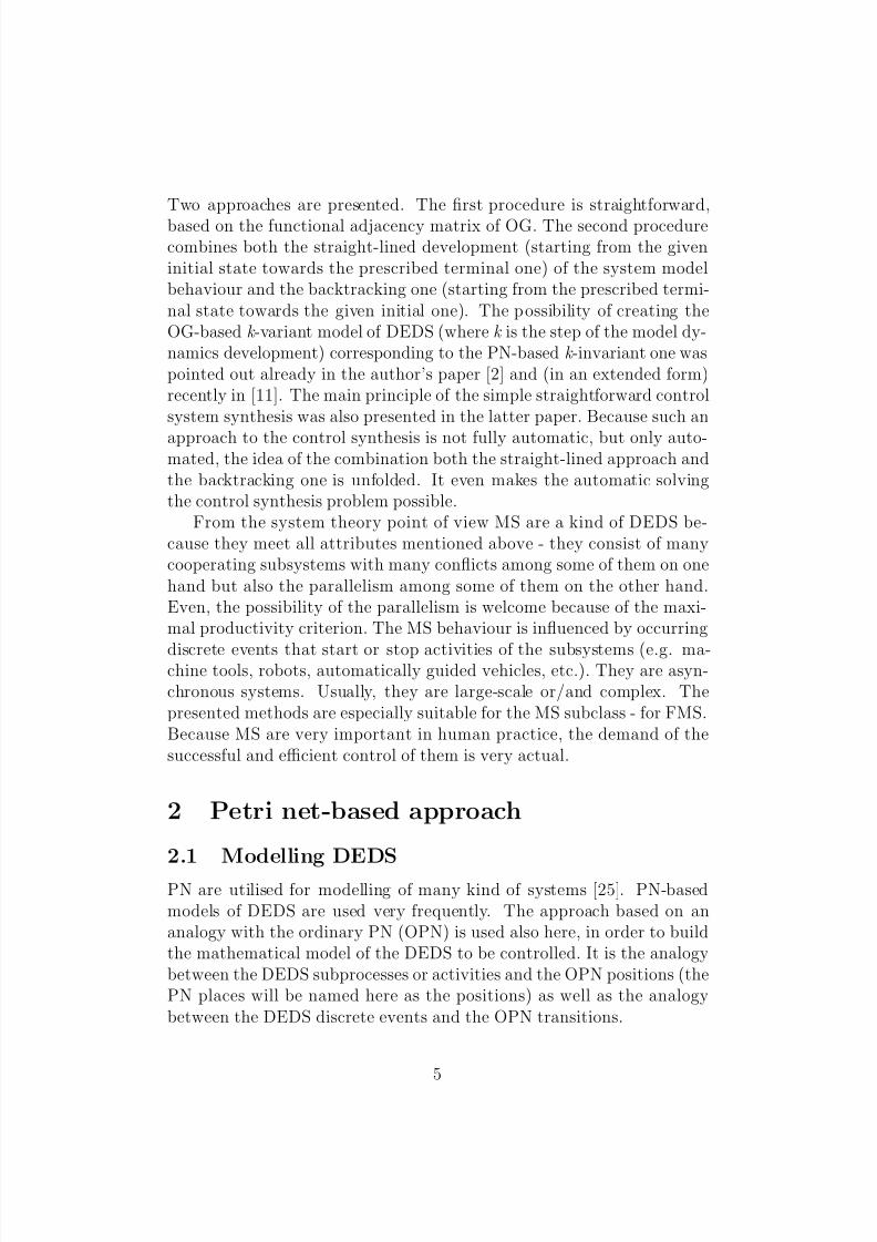
Two approaches are presented. The first procedure is straightforward,based on the functional adjacency matrix of OG. The second procedurecombines both the straight-lined development (starting from the giveninitial state towards the prescribed terminal one) of the system modelbehaviour and the backtracking one (starting from the prescribed termi-nal state towards the given initial one). The possibility of creating theOG-based k -variant model of DEDS (where k is the step of the model dy-namics development) corresponding to the PN-based k -invariant one waspointed out already in the author’s paper [2] and (in an extended form)recently in [11]. The main principle of the simple straightforward controlsystem synthesis was also presented in the latter paper. Because such an
approach to the control synthesis is not fully automatic, but only auto-mated, the idea of the combination both the straight-lined approach andthe backtracking one is unfolded. It even makes the automatic solvingthe control synthesis problem possible.
From the system theory point of view MS are a kind of DEDS be-cause they meet all attributes mentioned above - they consist of manycooperating subsystems with many conflicts among some of them on onehand but also the parallelism among some of them on the other hand.Even, the possibility of the parallelism is welcome because of the maxi-mal productivity criterion. The MS behaviour is influenced by occurring
discrete events that start or stop activities of the subsystems (e.g. ma-chine tools, robots, automatically guided vehicles, etc.). They are asyn-chronous systems. Usually, they are large-scale or/and complex. Thepresented methods are especially suitable for the MS subclass - for FMS.Because MS are very important in human practice, the demand of thesuccessful and efficient control of them is very actual.
2 Petri net-based approach
2.1 Modelling DEDS
PN are utilised for modelling of many kind of systems [25]. PN-basedmodels of DEDS are used very frequently. The approach based on ananalogy with the ordinary PN (OPN) is used also here, in order to buildthe mathematical model of the DEDS to be controlled. It is the analogybetween the DEDS subprocesses or activities and the OPN positions (thePN places will be named here as the positions) as well as the analogybetween the DEDS discrete events and the OPN transitions.
5

8/7/2019 Modelling and Control of Discrete Event Dynamic Systems
http://slidepdf.com/reader/full/modelling-and-control-of-discrete-event-dynamic-systems 8/61
2.1.1 The model structure
The OPN are understood here (as to their structure) to be the directedbipartite graphs
P , T , F , G ; P ∩ T = ∅ ; F ∩ G = ∅ (1)
whereP = p1,...,pn is a finite set of the OPN positions with pi , i = 1, n,
being the elementary positions.T = t1,...,tm is a finite set of the OPN transitions with tj , j =
1, m, being the elementary transitions.
F ⊆ P × T is a set of the oriented arcs entering the transitions. Itcan be expressed by means of the arcs incidence matrix F = f ij , f ij ∈0, M f ij , i = 1, n ; j = 1, m. The element f ij represents the absence(when 0) or presence and multiplicity M f ij (when M f ij > 0) of the arcoriented from the position pi to its output transition tj .
G ⊆ T × P is a set of the oriented arcs emerging from thetransitions. It can be expressed by means of the arcs incidence matrixG = gij , gij ∈ 0, M gij , i = 1, m ; j = 1, n.
The element gij represents analogically (to the matrix F) the absenceor presence and multiplicity of the arc oriented from the transition ti to
its output position pj .∅ is an empty set.
2.1.2 The model dynamics
However, OPN have not only their structure but also their dynamics - i.e.marking of their positions and its dynamic development. It can formallybe expressed by another quadruplet
X,U,δ, x0 ; X ∩ U = ∅ (2)
whereX = x0, x1..., xN is a finite set of the state vectors with xk , k =
0, N , being the elementary state vectors. Here, xk = (σkp1
, ..., σkpn
)T isthe n-dimensional state vector (marking) of the OPN-based model inthe step k of the system dynamics development. The element σk
pi∈
0, cpi, i = 1, n is the state of the elementary position pi in the step k- i.e. the passivity (when 0) or activity (when 0 < σk
pi≤ cpi), where cpi
is the capacity of the position pi. (.)T symbolises the matrix or vectortranspose.
6
8/7/2019 Modelling and Control of Discrete Event Dynamic Systems
http://slidepdf.com/reader/full/modelling-and-control-of-discrete-event-dynamic-systems 9/61
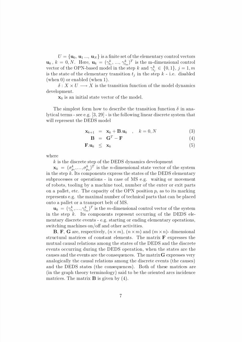
U = u0, u1 ..., uN is a finite set of the elementary control vectorsuk , k = 0, N . Here, uk = (γ kt1 , ..., γ ktm)T is the m-dimensional controlvector of the OPN-based model in the step k and γ ktj ∈ 0, 1, j = 1, mis the state of the elementary transition tj in the step k - i.e. disabled(when 0) or enabled (when 1).
δ : X × U −→ X is the transition function of the model dynamicsdevelopment.
x0 is an initial state vector of the model.
The simplest form how to describe the transition function δ in ana-lytical terms - see e.g. [3, 29] - is the following linear discrete system that
will represent the DEDS model
xk+1 = xk + B.uk , k = 0, N (3)
B = GT − F (4)
F.uk ≤ xk (5)
wherek is the discrete step of the DEDS dynamics developmentxk = (σk
p1,...,σk
pn)T is the n-dimensional state vector of the system
in the step k. Its components express the states of the DEDS elementary
subprocesses or operations - in case of MS e.g. waiting or movementof robots, tooling by a machine tool, number of the enter or exit partson a pallet, etc. The capacity of the OPN position pi as to its markingrepresents e.g. the maximal number of technical parts that can be placedonto a pallet or a transport belt of MS.
uk = (γ kt1 ,...,γ ktm)T is the m-dimensional control vector of the systemin the step k. Its components represent occurring of the DEDS ele-mentary discrete events - e.g. starting or ending elementary operations,switching machines on/off and other activities.
B, F, G are, respectively, (n × m), (n × m) and (m × n)- dimensional
structural matrices of constant elements. The matrix F expresses themutual causal relations among the states of the DEDS and the discreteevents occurring during the DEDS operation, when the states are thecauses and the events are the consequences. The matrix G expresses veryanalogically the causal relations among the discrete events (the causes)and the DEDS states (the consequences). Both of these matrices are(in the graph theory terminology) said to be the oriented arcs incidencematrices. The matrix B is given by (4).
7

8/7/2019 Modelling and Control of Discrete Event Dynamic Systems
http://slidepdf.com/reader/full/modelling-and-control-of-discrete-event-dynamic-systems 10/61
2.2 The control synthesis
The control synthesis problem is that of finding the most suitable se-quence (with respect to the control task specifications) of the controlvectors uk, k = 0, N that is able to transform the controlled systemfrom the given initial state x0 to a prescribed terminal state xt. Howeveras a rule, the DEDS control policy cannot be expressed analytically in aclosed form like in CTS or DTS. Namely, the control task specifications(e.g. constraints, criteria, etc.) are usually expressed only verbally. Con-sequently, in order to quantify the specifications the proper knowledgerepresentation (e.g. the rule-based one) is needed - see [3] - in the form
of a domain oriented knowledge base. The knowledge base is utilised atthe choice of the most suitable control vector uk in any step k when thereare several possibilities at disposal (in order to avoid any ambiguity asto the further development of the DEDS dynamics).
2.2.1 The verbal flowchart of the procedure
In order to find the suitable control vector uk able to transform thesystem from the existing state xk into a following state xk+1 the simpleprocedure can be used. It can be concisely described as follows:
START
• k = 0 i.e. xk = x0; x0 is an initial state; xt is a terminal state
LABEL:
• generation of the control base wk
• generation of the possible control vectors uk ∈ wk
• generation of the corresponding model responses xk+1
• consideration of the possibilities in the knowledge base (built on
IF-THEN rules and expressing the control task specifications)
• choice of the most suitable control possibility
• if (the xt or another stable state was found) then (goto END) else( begin k = k + 1 ; goto LABEL; end )
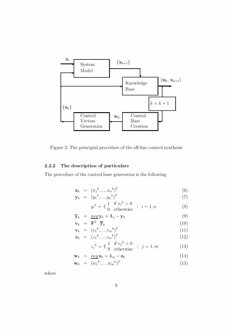
ENDThis procedure is schematically illustrated on Fig. 2.
8
8/7/2019 Modelling and Control of Discrete Event Dynamic Systems
http://slidepdf.com/reader/full/modelling-and-control-of-discrete-event-dynamic-systems 11/61
E
E
E
'' '
k = k + 1
ControlVectorsGeneration
ControlBaseCreation
Knowledge
Base
System
Modelc
aEa
wk
uk
(uk, xk+1)
xk+1xt
Figure 2: The principial procedure of the off-line control synthesis
2.2.2 The description of particulars
The procedure of the control base generation is the following
xk = (x1k,...,xn
k)T (6)
yk = (y1k,...,yn
k)T (7)
yik =
1 if xik > 0
0 otherwise; i = 1, n (8)
yk = neg yk = 1n − yk (9)
vk = FT . yk (10)
vk = (v1k
,...,vmk
)T
(11)zk = (z1
k,...,zmk)T (12)
zjk =
1 if vjk > 0
0 otherwise; j = 1, m (13)
wk = neg zk = 1m − zk (14)
wk = (w1k,...,wm
k)T (15)
where
9

8/7/2019 Modelling and Control of Discrete Event Dynamic Systems
http://slidepdf.com/reader/full/modelling-and-control-of-discrete-event-dynamic-systems 12/61
neg is the operator of logical negation.1n is the n-dimensional constant vector with all of its elements
equalled to the integer 1.yk is n-dimensional auxiliary vector with binary elements..vk, zk are, respectively, m-dimensional auxiliary vector and m-
dimensional auxiliary vector with binary elements.wk is m-dimensional vector of the base for the control vector choice.
The nonzero elements of the vector yk point out the active positions. Thenonzero elements of the vector yk point out the passive positions. Thenonzero elements of the vector zk point out the transitions having at leastone passive position among their input positions. Hence, such transitions
are disabled and from the control policy point of view they are out of thefield of our interest. The nonzero elements of the vector wk point outthe OPN transitions that can theoretically (potentially) be enabled inthe step k - i.e. on the possible discrete events which could occur in theDEDS in the step k and which could be utilised in order to transfer thesystem from the present state xk into another state xk+1. The vector wk
represents the control base because it expresses the possible candidatesfor generating the control vectors uk in the step k.
The above described procedure eliminates all disabled transitions.When only one of the wk components is different from zero, it can be
(when (5) is met, of course) used to be the control vector, i.e. uk = wk.The same is valid when wk has more components but the condition (5) isfulfilled. The maximal parallelism is welcome in MS. When the condition(5) is not met and there are several components of the wk different fromzero, the most suitable control vector uk has to be chosen on the base of additional information about the actual control task. The choice of thecontrol vector can be made either by a human operator or automaticallyon the base of a corresponding domain oriented knowledge representationbuilt in the form of the rules (e.g. IF-THEN ones) predefined by anexpert in the corresponding domain. Such a knowledge base consists of a
suitable expression of the constraints imposed upon the activities of thecontrolled system in question, control criteria, and further particularsconcerning the control task.
In general, to obtain the elementary control vectors uk ∈ wk thefollowing procedure is performed
uk = (u1k, ..., um
k)T
uk ⊆ wk (16)
10

8/7/2019 Modelling and Control of Discrete Event Dynamic Systems
http://slidepdf.com/reader/full/modelling-and-control-of-discrete-event-dynamic-systems 13/61
uj
k
=
wjk if chosen
0 otherwise ; j = 1, m (17)
Theoretically (i.e. from the combinatorics point of view) there exist
N pk =
N tk
i=1
N t
k
i
= 2N t
k
− 1 (18)
possibilities of the control vector choice in the step k. Here,
N tk =
mj=1
wjk. (19)
It means that there are the control vectors containing single nonzeroelements of the base vector wk, the control vectors containing pairs of itsnonzero elements, triples, quadruplets of its nonzero elements, etc., untilthe vector containing all of the nonzero elements of the base vector wk.
2.3 Knowledge representation
On the base of the above described control synthesis procedure, it isevident that a suitable form of the knowledge representation is neededin order to decide which control possibility should be actually chosen in
any step k. To construct a suitable knowledge base (KB) the rule-basedknowledge representation is usual in practice. The PN-based approachis used here in order to express the KB, even in analytical terms. It issupported by the logical PN (LPN) or/and fuzzy PN (FPN) - defined in[22], [23] and improved in [15].
2.3.1 The knowledge structure
Under the notion knowledge we mean some pieces of knowledge (somestatements) mutually connected by causal interconnections in the formof IF-THEN rules. The statements are expressed by the LPN/FPN po-
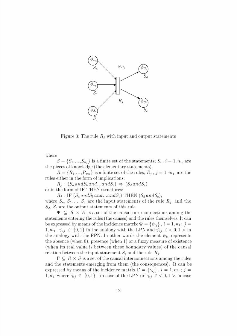
sitions and the rules are expressed by the LPN/FPN transitions (takentogether with their input and output positions). The mutual causalityinterconnections among the statements and rules are expressed by meansof the analogy with the oriented arcs among the PN positions and tran-sitions - see Fig. 3. More details about such a knowledge representationcan be found in [4]-[10]. Consequently, the KB structure can be formallyexpressed as
S,R, Ψ, Γ ; S ∩ R = ∅ ; Ψ ∩ Γ = ∅ (20)
11
8/7/2019 Modelling and Control of Discrete Event Dynamic Systems
http://slidepdf.com/reader/full/modelling-and-control-of-discrete-event-dynamic-systems 14/61
S c
S b
S a
S e
S d
φS c
φS b
φS a
φS e
φS d
Rj
ωRj
E
d d
d d
d ¨ B
r r r r r j
Figure 3: The rule Rj with input and output statements
whereS = S 1,...,S n1 is a finite set of the statements; S i , i = 1, n1, are
the pieces of knowledge (the elementary statements).R = R1,...,Rm1
is a finite set of the rules; Rj , j = 1, m1, are the
rules either in the form of implications:Rj : (S a andS b and...andS c) ⇒ (S d andS e)
or in the form of IF-THEN structures:Rj : IF (S a andS b and...andS c) THEN (S d andS e),
where S a, S b, ..., S c are the input statements of the rule Rj, and theS d, S e are the output statements of this rule.
Ψ ⊆ S × R is a set of the causal interconnections among thestatements entering the rules (the causes) and the rules themselves. It canbe expressed by means of the incidence matrix Ψ = ψij , i = 1, n1 ; j =1, m1. ψij ∈ 0, 1 in the analogy with the LPN and ψij ∈ < 0, 1 > in
the analogy with the FPN. In other words the element ψij representsthe absence (when 0), presence (when 1) or a fuzzy measure of existence(when its real value is between these boundary values) of the causalrelation between the input statement S i and the rule Rj.
Γ ⊆ R × S is a set of the causal interconnections among the rulesand the statements emerging from them (the consequences). It can beexpressed by means of the incidence matrix Γ = γ ij , i = 1, m1 ; j =1, n1, where γ ij ∈ 0, 1 , in case of the LPN or γ ij ∈ < 0, 1 > in case
12

8/7/2019 Modelling and Control of Discrete Event Dynamic Systems
http://slidepdf.com/reader/full/modelling-and-control-of-discrete-event-dynamic-systems 15/61
of the FPN. γ ij expresses the occurrence of the causal relation betweenthe rule Ri and its output statement S j (i.e. the absence, presence or afuzzy measure of existence).
2.3.2 The knowledge dynamics
The KB dynamics development (i.e. the statements truth propagation)can be formally expressed as follows
Φ, Ω, δ1, Φ0 ; Φ ∩ Ω = ∅ (21)
where
Φ = Φ0, Φ1..., ΦN 1 is a finite set of the KB elementary state vec-tors ΦK , K = 0, N 1. Here, ΦK = (φK
S 1, ..., φK
S n1)T is the n1-dimensional
state vector of the statements truth propagation in the step K . φK S i
∈0, 1, i = 1, n1 is the state of the elementary statement S i in the step K - i.e. in the case of using the LPN-based model - true (when 1) or false(when 0). In the case of using the FPN-based model φK
S i∈ < 0, 1, >, i =
1, n1 and it expresses the fuzzy measure of the statement truth. K is thestep of the KB dynamics development.
Ω = Ω0, Ω1 ..., ΩN 1 is a finite set of the KB elementary controlvectors ΩK , K = 0, N 1 expressing the state of the KB rules enabling.
Here, Ωk = (ωK R1, ..., ω
K Rm1 )
T
is the m1-dimensional control vector of theKB in the step k. ωK
Rj∈ 0, 1, j = 1, m1 is the state of the rule Rj
enabling in the step K - i.e. disabled (when 0) or enabled (when 1). Infuzzy case ωK
Rj∈ < 0, 1 >, j = 1, m1 and it expresses the fuzzy measure
of the rule enabling.δ1 : Φ × Ω −→ Φ is the transition function of the KB dynamics
development.Φ0 is an initial state vector of the KB.
The simplest form how to describe the transition function δ1 in ana-
lytical terms is the following linear logical system that will represent theKB model.
ΦK +1 = ΦK or ∆ and ΩK , K = 0, N 1 (22)
∆ = ΓT or Ψ (23)
Ψ and ΩK ≤ ΦK (24)
where
13

8/7/2019 Modelling and Control of Discrete Event Dynamic Systems
http://slidepdf.com/reader/full/modelling-and-control-of-discrete-event-dynamic-systems 16/61
S c
S b
S a
S e
S d
x
x
x
Rj
ωRj= 0
E
d d
d d
d ¨ B
r r r r r j
Figure 4: The enabled logical rule Rj
and is the operator of logical multiplying in general. For both thebivalued logic and the fuzzy one it can be defined (for scalar operands) tobe the minimum of its operands. For example the result of its applicationon the scalar operands a, b is a scalar c which can be obtained as follows:
aandb = c = mina, b.or is the operator of logical additioning in general. For both the
bivalued logic and the fuzzy one it can be defined (for scalar operands) tobe the maximum of its operands. For example the result of its applicationon the scalar operands a, b is a scalar c which can be obtained as follows :a o r b = c = maxa, b.
2.4 The knowledge inference
The procedure of the knowledge inference is very analogical to that for
obtaining the above introduced control base vector wK . It is the following
ΦK = neg ΦK = 1n1 − ΦK (25)
vK = ΨT and ΦK (26)
ΩK = neg vK = 1m1− vK =
= neg(ΨT and (neg ΦK )) (27)
where
14

8/7/2019 Modelling and Control of Discrete Event Dynamic Systems
http://slidepdf.com/reader/full/modelling-and-control-of-discrete-event-dynamic-systems 17/61
S c
S b
S a
S e
S d
x
x
x
x
x
Rj
ωRj= 1
E
d d
d d
d ¨ B
r r r r r j
Figure 5: The logical rule Rj after firing
S c
S b
S a
S e
S d
0.8
0.7
0.6
0.0
0.0
Rj
ωRj= 0.0
E
d d
d d
d ¨ B
r r r r r j
Figure 6: The enabled fuzzy rule Rj
15

8/7/2019 Modelling and Control of Discrete Event Dynamic Systems
http://slidepdf.com/reader/full/modelling-and-control-of-discrete-event-dynamic-systems 18/61
S c
S b
S a
S e
S d
0.8
0.7
0.6
0.3
0.3
Rj
ωRj= 0.3
E
d d
d d
d ¨ B
r r r r r j
Figure 7: The fuzzy rule Rj after firing
vK is the m1-dimensional auxiliary logical vector pointing out (byits nonzero elements) the rules that cannot be evaluated, because thereis at least one false (of course in the LPN analogy) statement among itsinput statements.
ΩK is the m1-dimensional ”control” vector pointing out the rulesthat have all their input statements true and, consequently, they can beevaluated in the step K of the KB dynamics development. This vector isa base of the inference, because it contains information about the rulesthat can contribute to obtaining the new knowledge - i.e. to transfer theKB from the state ΦK of the truth propagation into another state ΦK +1.The rules are pointed out by the nonzero elements of the vector ΩK .
neg is the operator of logical negation in general. For both thebivalued logic and the fuzzy one it can be defined (for scalar operands)to be the complement of its operand. For example : neg a = b = 1 − a.
2.5 Graphical tools
To automatise the model creating and testing as well as the process of theknowledge-based control synthesis the graphical tools were developed.
16

8/7/2019 Modelling and Control of Discrete Event Dynamic Systems
http://slidepdf.com/reader/full/modelling-and-control-of-discrete-event-dynamic-systems 19/61
2.5.1 The tool for the model drawing and testing
The graphical editor for drawing and testing the PN-based models is ableto draw ordinary PN, to compute their invariants, to draw their reacha-bility tree, to test their properties and to display the marking dynamicsdevelopment (token player). In addition to this it is able to draw the log-ical and fuzzy PN-based models, the time and timed PN-based models(see e.g. [17, 18]) and to display their marking dynamics development.It was developed during works on Master Theses [1],[24],[16]. To illus-trate some of its abilities, the following figures (see Fig. 8 - Fig. 13) areintroduced.
2.5.2 The tool for the knowledge-based control synthesis
In order to automatise the control synthesis process as well as in order tobridge the OPN-based model with the LPN/FPN-based KB the programsystem (knowledge-based control synthesiser) was created in the MasterThesis [12]. It makes possible to express relations between the statesof DEDS on one hand and the statements and rules of the KB on theother hand. It is user friendly and makes possible to simplify the work of the operator performing the DEDS control synthesis. Using the programsystem correctly, the control synthesis process can be fully automatised
(even automatic).Two files can be opened in the system - the OPN-based model (in the
form of a file like ’model-name.pnt’) created by means of the graphicaleditor of OPN mentioned above and the LPN/FPN-based KB (in theform of a file like ’kb-name.pnt’) created by means of the same graphi-cal editor by means of LPN/FPN. During the program system operationthree windows are on the screen - see Fig. 14 or Fig. 15. The KB oper-ates if the button KB is switched on. In the left window on the screenthe OPN-based model is displayed (the graphical model or its verbal de-scription can be alternatively seen). In the right window the LPN/FPN
model of the KB or the I/O interface between OPN model and the KBcan alternatively be seen. The I/O interface yields (at the beginningof its utilising) the empty skeleton corresponding to the number of thestatements and rules of the KB. It can be fulfilled by the operator inorder to define desirable relations between the OPN-based model andthe LPN/FPN-based KB. For example in the case of the KB with onlyone rule with two input and one output statements the skeleton is thefollowing:
17

8/7/2019 Modelling and Control of Discrete Event Dynamic Systems
http://slidepdf.com/reader/full/modelling-and-control-of-discrete-event-dynamic-systems 20/61
Figure 8: The example of the ordinary PN-based model.
Figure 9: The reachability tree of this model.
18

8/7/2019 Modelling and Control of Discrete Event Dynamic Systems
http://slidepdf.com/reader/full/modelling-and-control-of-discrete-event-dynamic-systems 21/61
Figure 10: The example of the logical PN-based model.
Figure 11: The example of the fuzzy PN-based model.
19

8/7/2019 Modelling and Control of Discrete Event Dynamic Systems
http://slidepdf.com/reader/full/modelling-and-control-of-discrete-event-dynamic-systems 22/61
Figure 12: The example of the time PN-based model.
Figure 13: The example of the timed PN-based model.
20

8/7/2019 Modelling and Control of Discrete Event Dynamic Systems
http://slidepdf.com/reader/full/modelling-and-control-of-discrete-event-dynamic-systems 23/61
Figure 14: A view on the screen of control synthesiser - the graphicalOPN model and the I/O interface.
input
P1
return F endP2
return F end
endoutput
// output place:// P3,return F
end
The third window (the state one) is placed in the down part of thescreen and it contains the actual state of the system as well as informationabout the enabled transitions of the OPN model. After finishing the
21

8/7/2019 Modelling and Control of Discrete Event Dynamic Systems
http://slidepdf.com/reader/full/modelling-and-control-of-discrete-event-dynamic-systems 24/61
Figure 15: The verbal description of the OPN and KB.
control synthesis process the final sequence of the control interferencesfor the real DEDS can be obtained from this window. When KB isswitched off, another small window appears in the center of the screen -see Fig. 16. It offers to the user the actual control possibilities and yieldshim the possibility to choose manually the most suitable one (from hissubjective point of view). The same window appears also in the casewhen KB works but it is not able to choose the most suitable possibility.In such a case the decision must be made by the human operator. Thedetail description of the program system is given in the user handbook[13].
2.6 The illustrative example
In order to illustrate the above introduced approach consider the FMSgiven on the Fig. 17. It can be seen that it consists of two robots servingfive machine tools, two automatic guided vehicles (AGVs), two entries(the inputs of raw materials A and B, respectively), and two exits (theoutputs of the final A-parts and B-parts, respectively). The machines 1and 2 produce the same intermediate A-parts and the machine 4 producesthe intermediate B-parts. Machines 3 and 5 produce the final A-parts
22

8/7/2019 Modelling and Control of Discrete Event Dynamic Systems
http://slidepdf.com/reader/full/modelling-and-control-of-discrete-event-dynamic-systems 25/61
Figure 16: The window for the manual choice. KB is switched off.
and B-parts, respectively. Using above mentioned analogy the OPN-based model can be obtained - see Fig. 18.
It can be knitted e.g. by means of the method elaborated and pre-sented in [14]. Meaning the OPN positions is the following:P1 - availability of A-raw material, P2 - loading by Robot 1 (R1), P3 -machining by Machine 1 (M1), P4 - delivering via AGV1, P5 - loadingby R2, P6 - machining by M3, P7 - machining by M2, P8 - availability of R1, P9 - availability of AGV1, P10 - availability of M1, P11 - availabilityof M2, P12 - availability of R2, P13 - availability of M3, P14 - loadingby R1, P15 - loading by R2, P16 - machining by M4, P17 - deliveringvia AGV2, P18 - machining by M5, P19 - availability of B-raw material,P20 - availability of M4, P21 - availability of AGV2, P22 - availability of
M5. The transitions T1 - T14 represent the starting or/and ending thecorresponding operations. The nonzero elements of the structural matri-ces of the OPN-based model are in case of the F : f 11, f 22, f 27, f 33, f 44,f 55, f 66, f 78, f 81, f 89, f 93, f 98, f 10,2, f 11,7, f 12,4, f 12,12, f 13,5, f 14,10, f 15,13,f 16,11, f 17,12, f 18,14, f 19,9, f 20,10, f 21,11, f 22,13 and in case of the G : g12,g23, g28, g34, g3,10, g45, g49, g56, g5,12, g61, g6,13, g77, g78, g84, g8,11, g9,14,g10,8, g10,16, g11,17, g11,20, g12,15, g12,21, g13,18, g13,12, g14,19, g14,22. The fullmatrices are not presented with regard to the limited space. Starting
23

8/7/2019 Modelling and Control of Discrete Event Dynamic Systems
http://slidepdf.com/reader/full/modelling-and-control-of-discrete-event-dynamic-systems 26/61
Figure 17: The flexible manufacturing system.
Figure 18: The OPN-based model of the FMS.
24

8/7/2019 Modelling and Control of Discrete Event Dynamic Systems
http://slidepdf.com/reader/full/modelling-and-control-of-discrete-event-dynamic-systems 27/61
from the initial state vector of the process
x0 = ( 1 0 0 0 0 0 0 1 1 1 1 1 1 0 0 0 0 0 1 1 1 1 )T
the following control base is obtained in the step k = 0
w0 = (1 0 0 0 0 0 0 0 1 0 0 0 0 0)T
Hence, the following control possibilities can be automatically generated
u10 = (1 0 0 0 0 0 0 0 0 0 0 0 0 0)T (28)
u20 = (0 0 0 0 0 0 0 0 1 0 0 0 0 0)T (29)
u30 = (1 0 0 0 0 0 0 0 1 0 0 0 0 0)T (30)
Only u30 does not satisfy the existence condition (5). It means that
remaining two possibilities are admissible, however, not simultaneously(R1 can take either A or B raw material). There is the conflict betweenthem (i.e. between the enabled transitions T1 and T9). The modelitself is not able to solve such a conflict because it has no informationabout it. To solve the conflict unambiguously external information (theintervention of the KB) is needed. The KB intervention should reflectboth the actual state of the system and the external conditions (EC)expressing the control task specifications (e.g. the actual state of storesof the A and B raw materials or/and actual requirements on the amountof the production of the A and B final parts). The form of a simplerule can be (in case of N p control possibilities) e.g. the following: IF
((u1k, x1
k+1) and ... and (uik, xi
k+1) and ... and (uN pk , x
N pk+1) and EC)
THEN (uik corresponding to the EC).
When (28) is chosen in the step k = 0 then
x1 = ( 0 1 0 0 0 0 0 0 1 1 1 1 1 0 0 0 0 0 1 1 1 1 )T
w1 = (0 1 0 0 0 0 1 0 0 0 0 0 0 0)T
Hence, three control possibilities can be automatically generated. How-ever, only two of them can be alternatively realized (R1 can serve eitherM1 or M2), namely
u11 = (0 1 0 0 0 0 0 0 0 0 0 0 0 0)T (31)
u21 = (0 0 0 0 0 0 1 0 0 0 0 0 0 0)T (32)
When the possibility (31) is chosen then
x2 = ( 0 0 1 0 0 0 0 1 1 0 1 1 1 0 0 0 0 0 1 1 1 1 )T
w2 = (1 0 1 0 0 0 0 0 1 0 0 0 0 0)T
25

8/7/2019 Modelling and Control of Discrete Event Dynamic Systems
http://slidepdf.com/reader/full/modelling-and-control-of-discrete-event-dynamic-systems 28/61
Consequently, seven control possibilities can be automatically generated.Five of them meet (5) and consequently, they can be separately realized.The following two ones must be eliminated
u52 = (1 0 0 0 0 0 0 0 1 0 0 0 0 0)T
u72 = (1 0 1 0 0 0 0 0 1 0 0 0 0 0)T
When (29) is chosen in the step k = 0 then
x1 = ( 1 0 0 0 0 0 0 0 1 1 1 1 1 1 0 0 0 0 0 1 1 1 )T
w1 = (0 0 0 0 0 0 0 0 0 1 0 0 0 0)T
Hence, only one control possibility is generated
u1 = (0 0 0 0 0 0 0 0 0 1 0 0 0 0)T
It can be accepted because it satisfies (5). Consequently,
x2 = ( 1 0 0 0 0 0 0 1 1 1 1 1 1 0 0 1 0 0 0 0 1 1 )T
w2 = (1 0 0 0 0 0 0 0 1 0 1 0 0 0)T
Hence, seven control possibilities can be automatically generated. Only
five of them are admissible as to (5), however, their simultaneous usingis excluded. The following two ones must be eliminated
u42 = (1 0 0 0 0 0 0 0 1 0 0 0 0 0)T
u72 = (1 0 0 0 0 0 0 0 1 0 1 0 0 0)T
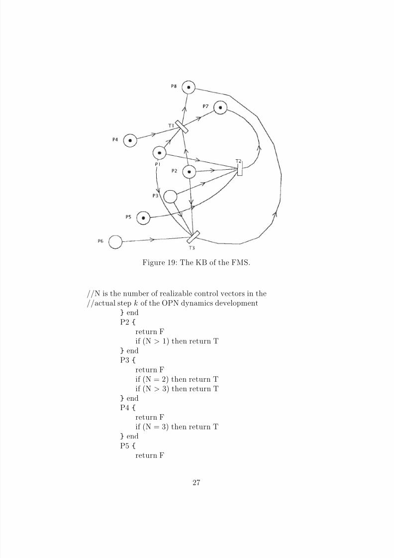
It can be seen that the process is branching very extensively. Toanalyse all possibilities manually is practically impossible. In situationswhen there are several equivalent possibilities (from the theoretical pointof view) how to choose the vector uk in a step k the domain oriented KByields the most suitable one (from the practical point of view). Let ususe the program system for the DEDS control synthesis. The proposedstructure of the KB is given by the Fig. 19 and proposed correspondinginterface is the following
input
P1
return Fif (N > 0) then return T
26
8/7/2019 Modelling and Control of Discrete Event Dynamic Systems
http://slidepdf.com/reader/full/modelling-and-control-of-discrete-event-dynamic-systems 29/61
Figure 19: The KB of the FMS.
//N is the number of realizable control vectors in the//actual step k of the OPN dynamics development
endP2
return Fif (N > 1) then return T
endP3
return Fif (N = 2) then return T
if (N > 3) then return T endP4
return Fif (N = 3) then return T
endP5
return F
27

8/7/2019 Modelling and Control of Discrete Event Dynamic Systems
http://slidepdf.com/reader/full/modelling-and-control-of-discrete-event-dynamic-systems 30/61
endP6
return F end
endoutput
// output places:// P7, P8
return 0if (N < 4) then
if (p.7=1) & (p.8=0) then return 1
if (p.7=0) & (p.8=1) then return 2if (p.7=1) & (p.8=1) then return 3
// p.j is the j-th component of the KB state vector
if (N > 3) then
if (p.7=1) & (p.8=0) then return 4if (p.7=0) & (p.8=1) then return 5
if (N = 1) then return 1 end
The result of the program operation (when maximal parallelism isutilised) in the case when number of the final parts A has the prioritywith respect to the number of the final parts B is given in Tab. 1 as thesequence of control interferences into the real DEDS.
3 Graph-based approaches for the state ma-
chines
For analytical modelling and control synthesis of DEDS that can be de-scribed by the special kind of PN - the so called state machines (whereany PN transition has only one input and only one output position)- theOG-based approaches are used.
3.1 The model based on the oriented graph
When the PN transitions are fixed on the corresponding oriented arcsamong the PN positions - see Fig. 20 - we have a structure that can be
28

8/7/2019 Modelling and Control of Discrete Event Dynamic Systems
http://slidepdf.com/reader/full/modelling-and-control-of-discrete-event-dynamic-systems 31/61
step k of dynamics OPN fired transitions
1 t12 t23 t3 & t94 t4 & t105 t5 & t116 t6 & t127 t1 & t138 t2 & t149 t3 & t9
. . . . . .
Table 1: The final results of the control synthesis.
understood to be the oriented graph. However, because the transitionfunctions of elementary transitions were functions, the oriented arcs willbe weighted by the functions too.
E E E
pj pitpi|pj
γ ktpi|pjσkpj σk
pi
Figure 20: An example of the placement of a transition on the orientedarc between two positions pi and pj
3.1.1 The model structure
The model structure can formally be described as
P, ∆ (33)
where
29

8/7/2019 Modelling and Control of Discrete Event Dynamic Systems
http://slidepdf.com/reader/full/modelling-and-control-of-discrete-event-dynamic-systems 32/61
P = p1,...,pn is a finite set of the OG nodes with pi , i = 1, n,being the elementary nodes. As a matter of fact they are the PN posi-tions.
∆ ⊆ P × P is a set of the OG edges i.e. the oriented arcs amongthe nodes. Its elements are represented by the functions expressing theoccurrence of the discrete events (represented above by the PN transi-tions). More precisely ∆ = ∆k ⊆ (P × T ) × (T × P ). It means thatthe PN transitions fixed on the oriented edges of the OG-based modelrepresent the model parameters while in the PN-based model they rep-resented the control vector. It is the principal difference between thePN-based model of DEDS and the OG-based one. The set ∆ can be ex-
pressed in the form of the incidence matrix ∆k = δkij , δkij ∈ 0, 1 , i =1, n , j = 1, n , k = 0, N . Its element δkij represents the absence (when 0)or presence (when 1) of the edge oriented from the node pi to the nodepj containing the PN transition. However, it is the transition functionand its value depends also on the step k. Namely, the correspondingtransition may be enabled in a step k1 but disabled in another step k2.
3.1.2 The model dynamics
The OG-based model dynamics can be formally expressed as follows
X, δ1, x0 (34)
where
X = x0, x1, ..., xN is a finite set of the state vectors of the graphnodes in different situations with xk = (σk
p1, ..., σk
pn)T , k = 0, N , being
the n-dimensional state vector of the graph nodes in the step k; σkpi
∈xk, i = 1, n is the state of the elementary node pi in the step k; k is thediscrete step of the OG-based model dynamics development.
δ1 : (X × U ) × (U × X ) −→ X is the transition function of thegraph dynamics. It contains implicitly the states of the transitions (theset U is the same like in the PN-based model dynamics) situated on theOG edges.
x0 is the initial state vector of the model dynamics.
30
8/7/2019 Modelling and Control of Discrete Event Dynamic Systems
http://slidepdf.com/reader/full/modelling-and-control-of-discrete-event-dynamic-systems 33/61
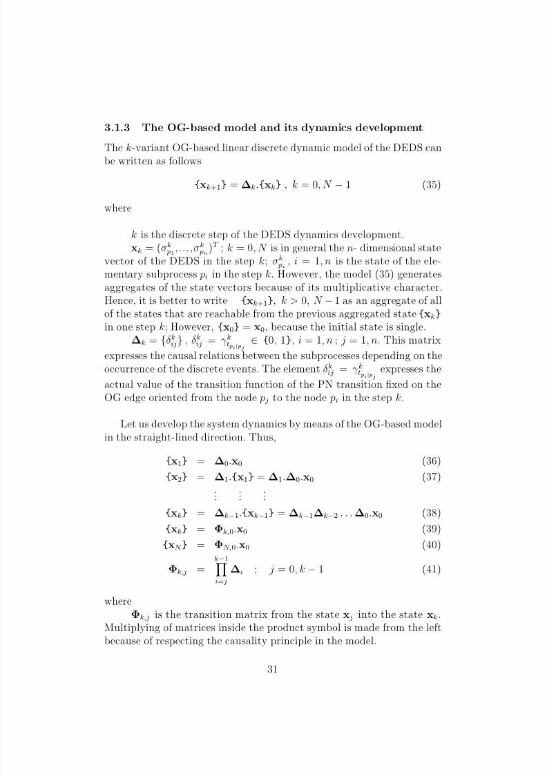
3.1.3 The OG-based model and its dynamics development
The k-variant OG-based linear discrete dynamic model of the DEDS canbe written as follows
xk+1 = ∆k.xk , k = 0, N − 1 (35)
where
k is the discrete step of the DEDS dynamics development.xk = (σk
p1,...,σk
pn)T ; k = 0, N is in general the n- dimensional state
vector of the DEDS in the step k; σkpi
, i = 1, n is the state of the ele-
mentary subprocess pi in the step k. However, the model (35) generatesaggregates of the state vectors because of its multiplicative character.Hence, it is better to write xk+1, k > 0, N − 1 as an aggregate of allof the states that are reachable from the previous aggregated state xk
in one step k; However, x0 = x0, because the initial state is single.∆k = δkij , δkij = γ ktpi|pj
∈ 0, 1, i = 1, n ; j = 1, n. This matrix
expresses the causal relations between the subprocesses depending on theoccurrence of the discrete events. The element δkij = γ ktpi|pj
expresses the
actual value of the transition function of the PN transition fixed on theOG edge oriented from the node pj to the node pi in the step k.
Let us develop the system dynamics by means of the OG-based modelin the straight-lined direction. Thus,
x1 = ∆0.x0 (36)
x2 = ∆1.x1 = ∆1.∆0.x0 (37)...
......
xk = ∆k−1.xk−1 = ∆k−1∆k−2 . . . ∆0.x0 (38)
xk = Φk,0.x0 (39)
xN = ΦN,0.x0 (40)
Φk,j =k−1i=j
∆i ; j = 0, k − 1 (41)
whereΦk,j is the transition matrix from the state xj into the state xk.
Multiplying of matrices inside the product symbol is made from the leftbecause of respecting the causality principle in the model.
31

8/7/2019 Modelling and Control of Discrete Event Dynamic Systems
http://slidepdf.com/reader/full/modelling-and-control-of-discrete-event-dynamic-systems 34/61
BE E
T
BE E T
BE E T
uk−1
xk−1Etuk−2
xk−2Et
u0
x0
xk E
...
Tx1Et
EE
EE
EE
t
t
T
...
xk
xk−1
x1x0
xk−2
xk−1
Φk,k−1
Φk−1,k−2
Φ1,0
Figure 21: The illustration of comparing the PN-based model (on theleft) and the OG-based one (on the right)
There is a symbolic interpretation as to the operators of multiplyingand additioning inside the matrices. The element φk,0
i,j ∈ Φk,0 has the
form of either a product of k elements (the transition functions expressingthe sequence of elementary transitions that must be fired in order to reachthe the final elementary state σk
pifrom the initial elementary state σ0
pj)
or a sum of several such products (when there are several ways how toreach the final state from the initial one). In the other words, any nonzeroelement δkij ∈ ∆k yields information about reachability of the state σk+1
pi
from the state σkpj
. Thus, any element φk2,k1i,j ∈ Φk2,k1 yields information
about the reachability of the state σk2pi
from the state σk1pj
.Both the PN-based model and the OG-based one are compared, as
to their structure, on Fig. 21. It can be seen that the former model is
strongly additive and it yields the actual states xi, i = 0, k (howeverthe control vectors ui, i = 0, k − 1 has to be known) while the latterone is strongly multiplicative and it yields only aggregates of the statevectors, however the actual values of the parameters need not be known.Such an OG-based approach to the control synthesis yields the analyticalsolution in the closed form.
32

8/7/2019 Modelling and Control of Discrete Event Dynamic Systems
http://slidepdf.com/reader/full/modelling-and-control-of-discrete-event-dynamic-systems 35/61
15
mouse
3
cat
4 2
rtv c6 rtvc3
rtvm4 rtv m1
rtvc7rtv
rtvc5
rtvm5
rtvm6
rtvc4 rtv
c1
rtvm3
rtvm2
rtvc2
Figure 22: The maze structure.
3.1.4 The illustrative example
Consider the maze problem introduced by Ramadge and Wonham in [31].Two participants - in [31] a cat and a mouse - can be as well e.g. twomobile robots or two AGVs of the FMS, two cars in a road network, twotrains in a railway network, etc. They are placed in the maze (however,it can also be e.g. a complicated crossroad, complicated railways points,crossing AGVs lines in FMS etc.) given on Fig. 22 consisting of five roomsdenoted by numbers 1, 2,..., 5 connecting by the doorways exclusively forthe cat denoted by ci, i = 1, 7 and the doorways exclusively for the mousedenoted by mj, j = 1, 6. The cat is initially in the room 3 and the mousein the room 5. Each doorway can be traversed only in the direction
indicated. Each door (with the exception of the door c7) can be openedor closed by means of control actions. The door c7 is uncontrollable(or better, it is continuously open in both directions). The controllerto be synthesised observes only discrete events generated by sensors inthe doors. They indicate that a participant is just running through.The control problem is to find a feedback controller (e.g. an automaticpoints-man or switchman in railways, a system of crossroad lights, etc.)such that the following control task specifications - three criteria or/and
33

8/7/2019 Modelling and Control of Discrete Event Dynamic Systems
http://slidepdf.com/reader/full/modelling-and-control-of-discrete-event-dynamic-systems 36/61
constraints will be satisfied:
1. The participants never occupy the same room simultaneously
2. It is always possible for both of them to return to their initialpositions (the first one to the room 3 and the second one to theroom 5)
3. The controller should enable the participants to behave as freely aspossible with respect to the constraints imposed.
It can be seen that the criteria and constraints are completely given in
the verbal form.At the construction of the PN-based model of the system the rooms
1 - 5 of the maze will be represented by the PN positions p1 - p5 and thedoorways will be represented by the PN transitions. The permanentlyopen door c7 is replaced by means of two PN transitions t7 and t8 sym-bolically denoted as ck7 and ck8 . The PN-based representation of the mazeis given on Figure 23. The initial state vectors of the cat and the mouseare
cx0 = (0 0 1 0 0) , mx0 = (0 0 0 0 1)T (42)
The structure of the cat and mouse control vectors is
cuk = (ck1, ck2, ck3, ck4, ck5, ck6, ck7, ck8)T ; cki ∈ 0, 1, i = 1, 8muk = (mk
1, mk2, mk
3, mk4, mk
5, mk6)T ; mk
i ∈ 0, 1, i = 1, 6
The parameters of the cat model are
n = 5 mc = 8
cF =
1 0 0 1 0 0 0 0
0 1 0 0 0 0 1 00 0 1 0 0 0 0 00 0 0 0 1 0 0 10 0 0 0 0 1 0 0
; cG =
0 1 0 0 00 0 1 0 01 0 0 0 00 0 0 1 00 0 0 0 11 0 0 0 00 0 0 1 00 1 0 0 0
and the parameters of the mouse model are
34

8/7/2019 Modelling and Control of Discrete Event Dynamic Systems
http://slidepdf.com/reader/full/modelling-and-control-of-discrete-event-dynamic-systems 37/61
m m
m
m m
m m
m
m mv
vp4 p5
p1
p2 p3
a)
p4 p5
p1
p2 p3
b)
rtv
rtv
rtv
rtv
rtv
rtv
rtv
rtv
rtv
rtvrtv
rtvd
d rtvrtv
rtv
rtv d
d rtv
d d d d d
d d d d d
d d d d d
d d d d d
rtv
rtv
rtv
rtv
rtv
rtvrtv
rtvd
d rtv rtv
rtv
d d rtv
ck2
ck5
ck7 ck8
ck1 ck3
ck4 ck6
mk2
mk5
mk3 mk
1
mk6 mk
4
Figure 23: The PN-based representation of the maze. a) possible be-haviour of the cat; b) possible behaviour of the mouse
n = 5 mm = 6
mF =
1 0 0 1 0 00 0 1 0 0 00 1 0 0 0 00 0 0 0 0 1
0 0 0 0 1 0
; mGT m =
0 0 1 0 0 10 1 0 0 0 01 0 0 0 0 00 0 0 0 1 0
0 0 0 1 0 0
At the construction of the OG-based model (see Fig. 24) the matricesc∆k and m∆k of the system parameters are the following
c∆k =
0 0 ck3 0 ck6ck1 0 0 ck8 00 ck2 0 0 0ck4 ck7 0 0 00 0 0 ck5 0
=
0 0 cδk13 0 cδk15cδk21 0 0 cδk24 0
0 cδk32 0 0 0cδk41
cδk42 0 0 00 0 0 cδk54 0
m∆k =
0 mk3 0 mk
6 00 0 mk
2 0 0mk
1 0 0 0 00 0 0 0 mk
5
mk4 0 0 0 0
=
35

8/7/2019 Modelling and Control of Discrete Event Dynamic Systems
http://slidepdf.com/reader/full/modelling-and-control-of-discrete-event-dynamic-systems 38/61
m m
m
m m
m m
m
m mv
vp4 p5
p1
p2 p3
a)
p4 p5
p1
p2 p3
b)
rtv
rtv
rtv
rtv
rtv
rtvrtv
rtv
d d d d d
d d d d d
d d d d d
d d d d d
rtv
rtv
rtv
rtvrtv
rtv
cδk32
cδk54
cδk42cδk24
cδk21cδk13
cδk41cδk15
mδk23
mδk45
mδk12mδk31
mδk14mδk51
Figure 24: The OG-based model of the maze. a) possible behaviour of the cat; b) possible behaviour of the mouse
=
0 mδk12 0 mδk14 00 0 mδk23 0 0
mδk31 0 0 0 00 0 0 0 mδk45
mδk51 0 0 0 0
The transitions matrices for the cat and mouse are the followingcΦk+2,k = c∆k+1.c∆k =
=
0 ck+13 .ck2 0 ck+16 .ck5 0ck+18 .ck4 ck+18 .ck7 ck+11 .ck3 0 ck+11 .ck6ck+12 .ck1 0 0 ck+12 .ck8 0ck+17 .ck1 0 ck+14 .ck3 ck+17 .ck8 ck+14 .ck6ck+15 .ck4 ck+15 .ck7 0 0 0
c
Φk+3,k =c
∆k+2.c
∆k+1.c
∆k =
=
ck+23 .ck+12 .ck1 + ck+26 .ck+15 .ck4 ck+26 .ck+15 .ck7...
ck+28 .ck+17 .ck1 ck+21 .ck+13 .ck2...
ck+22 .ck+18 .ck4 ck+22 .ck+18 .ck7...
ck+27 .ck+18 .ck4 ck+24 .ck+13 .ck2 + ck+27 .ck+18 .ck7...
ck+25 .ck+17 .ck1 0...
36

8/7/2019 Modelling and Control of Discrete Event Dynamic Systems
http://slidepdf.com/reader/full/modelling-and-control-of-discrete-event-dynamic-systems 39/61
..
. 0 c
k+2
3 .c
k+1
2 .c
k
8 0... ck+28 .ck+14 .ck3 ck+21 .ck+16 .ck5 + ck+28 .ck+12 .ck8 ck+28 .ck+14 .ck6... ck+22 .ck+11 .ck3 0 ck+22 .ck+11 .ck6... ck+27 .ck+11 .ck3 ck+24 .ck+16 .ck5 ck+27 .ck+11 .ck6... ck+25 .ck+14 .ck3 ck+25 .ck+17 .ck8 ck+25 .ck+14 .ck6
mΦk+2,k = m∆k+1.m∆k =
=
0 0 mk+13 .mk
2 mk+16 .mk
5
m
k+1
2 .m
k
1 0 0 0 00 mk+11 .mk
3 0 mk+11 .mk
6 0mk+1
5 .mk4 0 0 0 0
0 mk+14 .mk
3 0 mk+14 .mk
6 0
mΦk+3,k = m∆k+2.m∆k+1.m∆k =
=
mk+23 .mk+1
2 .mk1 + mk+2
6 .mk+15 .mk
4 0...
0 mk+22 .mk+1
1 .mk3
...
0 0...
0 mk+25 .mk+1
4 mk3 ...
0 0...
... 0 0 0
... 0 mk+22 .mk+1
1 .mk6 0
... mk+21 .mk+1
3 .mk2 0 mk+2
1 .mk+16 .mk
5
... 0 mk+25 .mk+1
4 .mk6 0
..
. mk+2
4 .mk+1
3 .mk
2 0 mk+2
4 .mk+1
6 .mk
5
The corresponding states reachability trees are given on Fig. 25 andFig. 26. It can be seen that in order to fulfil the prescribed controltask specifications introduced above, the comparison of the transitionmatrices of both animals in any step of their dynamics development issufficient. Because the animals start from the defined rooms given bytheir initial states, it is sufficient to compare the columns 3 and 5. Con-sequently,
37

8/7/2019 Modelling and Control of Discrete Event Dynamic Systems
http://slidepdf.com/reader/full/modelling-and-control-of-discrete-event-dynamic-systems 40/61
c03
(0, 0, 1, 0, 0)
(1, 0, 0, 0, 0)
d d
d d
c11
c14
(0, 1, 0, 0, 0) (0, 0, 0, 1, 0)
d d d d
c22 c27
(0, 0, 1, 0, 0) (0, 0, 0, 1, 0)
d d d d
c25 c28
(0, 0, 0, 0, 1) (0, 1, 0, 0, 0)
. . . . . . . . . . . . . . . . . . . . . . . .
Figure 25: The fragment of the reachability tree of the cat
m05
(0, 0, 0, 0, 1)
(0, 0, 0, 1, 0)
m16
(1, 0, 0, 0, 0)
d
d d d
m21 m24
(0, 0, 1, 0, 0) (0, 0, 0, 0, 1)
. . . . . . . . . . . .
Figure 26: The reachability tree of the mouse
38

8/7/2019 Modelling and Control of Discrete Event Dynamic Systems
http://slidepdf.com/reader/full/modelling-and-control-of-discrete-event-dynamic-systems 41/61
1. the corresponding (as to indices) elements of the transition matricesin these columns have to be mutually disjunct in any step of thedynamics development in order to avoid encounter of the animalson the corresponding trajectories.
2. if they are not disjunct one of them must be removed. It dependson the control task specifications which one will be removed. Let usgo to focus attention on the elements with indices [3,3] and [5,5] of the matrices Φk+3,0. Namely, they express the trajectories makingthe return of the animals to their initial states possible. In case of the elements with indices [3,3] the element of the matrix cΦk+3,0
should be chosen. It represents the trajectory of the cat makingtheir come back possible. In case of the elements with indices [5,5]the element of the matrix mΦk+3,0 should be chosen. It representsthe trajectory of the mouse making their come back possible.
3. in the matrix cΦk+3,k two elements in the column 3 (with the indices[2,3] and [4,3]) stay unremoved, because of the permanently opendoor. It can be seen that also the elements of the column 5 of this matrix (with indices [2,5] and [4,5]) stay unremoved. Thisfacts correspond with the prescribed condition 3 in the control taskspecifications.
On the base of these particulars it is clear that the KB construction neednot be very complicated. In any case it is easier than that required bythe OPN-based model at the knowledge-based approach to the controlsynthesis, because it is sufficient here to check only the actual elementsof the transition matrices.
3.2 The combined approach to the control synthesis
The main disadvantage of the previous approach is the consumption of
much memory because of the functional matrices - the functional adja-cency matrix and its powers. It should be more suitable to work withthe classical numerical adjacency matrix. Below such an approach is pro-posed. The adjacency matrix helps to generate automatically the statereachability tree in both the straight-lined system development (from aninitial state towards the prescribed terminal one) and that of the back-tracking system development (from the terminal state towards the initialone). To perform the DEDS control synthesis the combination both of
39

8/7/2019 Modelling and Control of Discrete Event Dynamic Systems
http://slidepdf.com/reader/full/modelling-and-control-of-discrete-event-dynamic-systems 42/61
these kinds of the model behaviour development is used. The coinci-dence (a suitable intersection) both of the state reachability trees yieldsthe possible trajectories of the system development. In such a way allsolutions how to reach the prescribed terminal state from the given ini-tial one are automatically found. To choose the most suitable solutionrule-based knowledge about the control task specifications can also beutilised. Sometimes it may be fuzzy.
3.2.1 The straight lined dynamics development
When the input vector xk represents a state of the system and we do not
know the actual state of the transition functions (i.e. the actual stateof the functional elements δkij of the k-variant matrix ∆k), we can usethe transpose of the classical (numerical) OG adjacency matrix - i.e. the
matrix ∆ = δij having the same structure like the matrix ∆k = δ(k)ij ,however its elements are not functional but they are defined as follows
∆ = δij; δij = 1 if δkij = 00 otherwise
; i = 1,n, j = 1, n (43)
It means that ∆ is the constant matrix with all elements correspondingwith the functional elements of the matrix ∆k equal to 1. Thus, in thebelow system development we can understand that ∆k = ∆, k = 0, N −1.Let us start to derive the approach from the following form of the modeldescription
xk+1 = ∆.xk , k = 0, N − 1 (44)
where xk+1 is an aggregate of all of the states that are reachable fromthe previous states xk in one step k. There is only one exceptionx0 = x0, because the given initial state is only single. There is onlyone difference here in comparison with the model (35). The matrix ∆
is the constant matrix (the transpose of the adjacency matrix). Let usdevelop the system dynamics in the straight-lined orientation. Hence,
x1 = ∆.x0 (45)x2 = ∆.x1 = ∆.(∆.x0) = ∆2.x0 (46)
......
...
xk = ∆.xk−1 = ∆.(∆k−1.x0) = ∆k.x0
xk = Φk,0.x0 (47)
Φk,j =k−1i=j
∆ (48)
40

8/7/2019 Modelling and Control of Discrete Event Dynamic Systems
http://slidepdf.com/reader/full/modelling-and-control-of-discrete-event-dynamic-systems 43/61
The multiplying is made from the left because of the causality principle.
3.2.2 The backtracking dynamics development
The procedure very analogical to that starting from the initial state x0
can start from the terminal state xt. Let us denote the terminal stateas xN . Using the functional matrix ∆k, in general the following relationcan be written
xN −k−1 = ∆T N −k−1.xN −k, k = 0, N − 1 (49)
wherexN −k−1 is an aggregate of all of the states from which the states
xN −k are reachable in one step k. There is only one exception xN =xN , because the terminal state is only single.
Consequently, the backtracking system development is the following
xN −1 = ∆T N −1.xN (50)
xN −2 = ∆T N −2.xN −1 = ∆T
N −2∆T N −1.xN (51)
......
......
......
...
x0 = ∆T 0 .x1 = ∆
T 0 ∆
T 1 . . . ∆
T N −2∆
T N −1.xN (52)
However, using the constant matrix ∆ we have in general
xN −k−1 = ∆T .xN −k, k = 0, N − 1 (53)
and the backtracking system development is the following
xN −1 = ∆T .xN (54)
xN −2 = ∆T .xN −1 = ∆T .(∆T .xN ) = (∆T )2.xN (55)..
.
..
.
..
.
..
.
..
.
..
.
..
.x0 = ∆T .x1 = ∆T .((∆T )N −1.xN ) = (∆T )N .xN (56)
3.2.3 The control synthesis by means of intersection
The main problem of the control synthesis is that usually there are sev-eral possibilities how to proceed in any step of the system dynamicsdevelopment. Consequently, there exists a tree of the possibilities of thesystem behaviour. The process of searching the most suitable path can
41
8/7/2019 Modelling and Control of Discrete Event Dynamic Systems
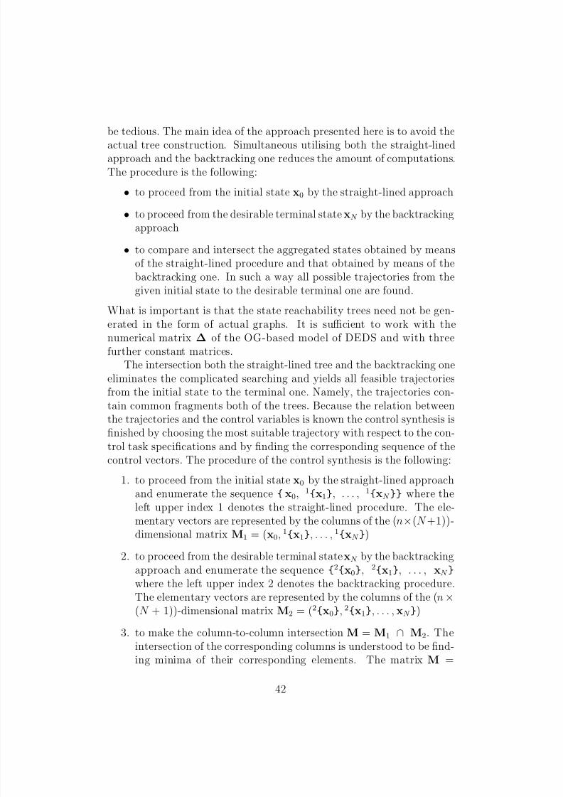
http://slidepdf.com/reader/full/modelling-and-control-of-discrete-event-dynamic-systems 44/61
be tedious. The main idea of the approach presented here is to avoid theactual tree construction. Simultaneous utilising both the straight-linedapproach and the backtracking one reduces the amount of computations.The procedure is the following:
• to proceed from the initial state x0 by the straight-lined approach
• to proceed from the desirable terminal state xN by the backtrackingapproach
• to compare and intersect the aggregated states obtained by meansof the straight-lined procedure and that obtained by means of the
backtracking one. In such a way all possible trajectories from thegiven initial state to the desirable terminal one are found.
What is important is that the state reachability trees need not be gen-erated in the form of actual graphs. It is sufficient to work with thenumerical matrix ∆ of the OG-based model of DEDS and with threefurther constant matrices.
The intersection both the straight-lined tree and the backtracking oneeliminates the complicated searching and yields all feasible trajectoriesfrom the initial state to the terminal one. Namely, the trajectories con-tain common fragments both of the trees. Because the relation between
the trajectories and the control variables is known the control synthesis isfinished by choosing the most suitable trajectory with respect to the con-trol task specifications and by finding the corresponding sequence of thecontrol vectors. The procedure of the control synthesis is the following:
1. to proceed from the initial state x0 by the straight-lined approachand enumerate the sequence x0, 1x1, . . . , 1xN where theleft upper index 1 denotes the straight-lined procedure. The ele-mentary vectors are represented by the columns of the (n×(N +1))-dimensional matrix M1 = (x0, 1x1, . . . , 1xN )
2. to proceed from the desirable terminal state xN by the backtrackingapproach and enumerate the sequence 2x0, 2x1, . . . , xN
where the left upper index 2 denotes the backtracking procedure.The elementary vectors are represented by the columns of the (n ×(N + 1))-dimensional matrix M2 = (2x0, 2x1, . . . , xN )
3. to make the column-to-column intersection M = M1 ∩ M2. Theintersection of the corresponding columns is understood to be find-ing minima of their corresponding elements. The matrix M =
42
8/7/2019 Modelling and Control of Discrete Event Dynamic Systems
http://slidepdf.com/reader/full/modelling-and-control-of-discrete-event-dynamic-systems 45/61
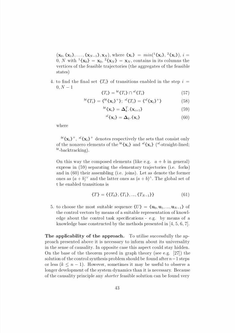
(x0, x1, . . . , xN −1, xN ), where xi = min(1xi, 2xi), i =0, N with 1x0 = x0, 2xN = xN , contains in its columns thevertices of the feasible trajectories (the aggregates of the feasiblestates)
4. to find the final set T i of transitions enabled in the step i =0, N − 1
T i = btT i ∩ sl
T i (57)
btT i =
btxi
+; sl
T i = slxi
+ (58)
btxi = ∆T
k .xi+1 (59)
slxi = ∆k.xi (60)
where
btxi+, slxi
+ denotes respectively the sets that consist onlyof the nonzero elements of the btxi and slxi (sl-straight-lined;bt-backtracking).
On this way the composed elements (like e.g. a + b in general)express in (59) separating the elementary trajectories (i.e. forks)
and in (60) their assembling (i.e. joins). Let as denote the formerones as (a + b)∨ and the latter ones as (a + b)∧. The global set of t he enabled transitions is
T = T 0, T 1, ...,T N −1 (61)
5. to choose the most suitable sequence U = u0, u1, ..., uN −1 of the control vectors by means of a suitable representation of knowl-edge about the control task specifications - e.g. by means of aknowledge base constructed by the methods presented in [4, 5, 6, 7].
The applicability of the approach. To utilise successfully the ap-proach presented above it is necessary to inform about its universalityin the sense of causality. In opposite case this aspect could stay hidden.On the base of the theorem proved in graph theory (see e.g. [27]) thesolution of the control synthesis problem should be found after n−1 stepsor less (k ≤ n − 1). However, sometimes it may be useful to observe alonger development of the system dynamics than it is necessary. Becauseof the causality principle any shorter feasible solution can be found very
43

8/7/2019 Modelling and Control of Discrete Event Dynamic Systems
http://slidepdf.com/reader/full/modelling-and-control-of-discrete-event-dynamic-systems 46/61
simply because it is involved in the longer one. Namely, when during theintersection of the matrices M1 and M2 the latter one is shifted to theleft for one column we obtain another matrix −1M with dimensionality(n × N ). It is the following
−1M = (x0, x1, . . . , xN −2, xN −1) (62)
wherexN −1 = xt (the same terminal state like before).
In general, the shifting (i.e. finding the [n × (N − k + 1)]-dimensionalmatrices −kM, k = 1, 2,...) can continue until the intersections exist, i.e.until x0 ∈ 2x0 and simultaneously xt ∈ 1xN −k.
3.2.4 A general view on the approach
The adjacency matrix ∆ is the non-negative matrix defined e.g. in[20, 28, 30]. The necessary condition for the above procedure has tobe fulfilled - namely, the terminal state xN must be reachable from theinitial state x0. It is not very difficult to test the reachability. For sucha testing the result of the proved theorem [20, 26, 27] can be used. Thetest is based on computation of the k-th power (where k is unknownbefore) of the OG adjacency matrix. Because we use the transpose ∆ of
the original adjacency matrix, to obtain ∆
k
containing the first nonzeroelement δkij we have to multiply the matrix ∆ from the left. The nonzeroelement δkij of the matrix ∆k gives us information not only about thereachability of the i-th element of the state vector xk from the j-th el-ement of the state vector x0 but also about the number of the steps kthat have to be performed (more mathematical details can be found inliterature [20, 26, 27]). How long is it necessary to compute the powersof the matrix? The question is answered in [27] - the exponent k ≤ n− 1.Of course, it is concerning only the reachability of a single position fromanother single one. The simultaneous reachability of several positions(the vector of the positions like the state vector in our case) from an-other vector of positions requires more steps. Because the higher powersof the adjacency matrix (that is nonnegative matrix) can be positivematrices, the following discussion is useful. The results on this way cancreate a base for a possible generalisation of the above introduced controlsynthesis procedure.
A discussion about the exponent k for the indecomposable ad-
jacency matrix. At the guess of the exponent k in special cases the re-
44

8/7/2019 Modelling and Control of Discrete Event Dynamic Systems
http://slidepdf.com/reader/full/modelling-and-control-of-discrete-event-dynamic-systems 47/61
sults published in [28, 30] concerning indecomposable non-negative n×n-dimensional matrices can be utilised. The indecomposable matrix is de-fined in [20] as the matrix which is not decomposable. The matrix A
is decomposable if it is of the following form (63) or if there exists apermutation matrix P such that PT AP is of the form (63)
A =
A11 A12
0/ A22
(63)
where submatrices Aii, i = 1, 2 are square matrices. 0/ is the zero matrixwith the corresponding dimensionality. A real matrix R is non-negativeif all its elements rij ≥ 0. When a power of the indecomposable non-negative n × n-dimensional matrix is a positive matrix (a real matrixQ is positive if all its elements qij > 0), the matrix is primitive (as it ismentioned in [28] this term was introduced by Frobenius in 1912). For thebest upper bound of the exponent kmin guaranteeing that correspondingpower of the primitive matrix (for n ≥ 2) is positive the inequality kmin ≤ωn = (n − 1)2 +1 is valid - see [28, 30]. Hence, at least one common statecan be found by both the straight-lined procedure and the backtrackingone after such a number of steps. The proposed combined approach tothe control synthesis seems to be powerful and may be promising forextension of its validity for a wider class of PN.
There are some new results for n ≥ 3 in [21] concerning the minimalexponent. It is proved that if kmin ≥ ωn/2 + 2 then the primitive di-rected graph has cycles of exactly two different lengths i, j with n ≥ j > i.Because in the graph theory - see e.g. [19] - the oriented and directed graphs are distinguished (the oriented graph is understood in [19] to bea directed graph having no symmetric pair of directed edges or in otherwords the directed graphs without loops or multiple edges) the new re-sults are partially applicable for our case. The adjacency matrix of theOG-based model of DEDS can be decomposable in general (and conse-quently, it will be imprimitive). However, the considerations analogical
to indecomposable matrix A can be done for the indecomposable sub-matrices Aii, i = 1, 2 of the decomposable matrix A.
3.2.5 The illustrative example
Consider the same maze problem introduced above. Its structure is givenon Fig. 22. The PN-based models for cat and mouse are given on Fig. 23and the OG-based models on Fig. 24. The parameters of the PN-basedmodels are introduced there too (the matrices cF, cG, mF, mG) as well
45
8/7/2019 Modelling and Control of Discrete Event Dynamic Systems
http://slidepdf.com/reader/full/modelling-and-control-of-discrete-event-dynamic-systems 48/61
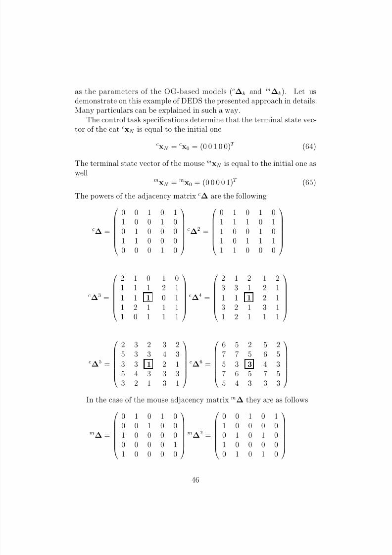
as the parameters of the OG-based models (c∆k and m∆k). Let usdemonstrate on this example of DEDS the presented approach in details.Many particulars can be explained in such a way.
The control task specifications determine that the terminal state vec-tor of the cat cxN is equal to the initial one
cxN = cx0 = (0 0 1 0 0)T (64)
The terminal state vector of the mouse mxN is equal to the initial one aswell
mxN = mx0 = (0 0 0 0 1)T (65)
The powers of the adjacency matrix c∆ are the following
c∆ =
0 0 1 0 11 0 0 1 00 1 0 0 01 1 0 0 00 0 0 1 0
c∆2 =
0 1 0 1 01 1 1 0 11 0 0 1 01 0 1 1 11 1 0 0 0
c∆3 =
2 1 0 1 0
1 1 1 2 11 1 1 0 11 2 1 1 11 0 1 1 1
c∆4 =
2 1 2 1 2
3 3 1 2 11 1 1 2 13 2 1 3 11 2 1 1 1
c∆5 =
2 3 2 3 25 3 3 4 3
3 3 1 2 15 4 3 3 33 2 1 3 1
c∆6 =
6 5 2 5 27 7 5 6 5
5 3 3 4 37 6 5 7 55 4 3 3 3
In the case of the mouse adjacency matrix m∆ they are as follows
m∆ =
0 1 0 1 00 0 1 0 01 0 0 0 00 0 0 0 11 0 0 0 0
m∆2 =
0 0 1 0 11 0 0 0 00 1 0 1 01 0 0 0 00 1 0 1 0
46

8/7/2019 Modelling and Control of Discrete Event Dynamic Systems
http://slidepdf.com/reader/full/modelling-and-control-of-discrete-event-dynamic-systems 49/61
m∆3 =
2 0 0 0 0
0 1 0 1 00 0 1 0 10 1 0 1 0
0 0 1 0 1
m∆4 =
0 2 0 2 0
0 0 1 0 12 0 0 0 00 0 1 0 12 0 0 0 0
m∆5 =
0 0 2 0 22 0 0 0 00 2 0 2 02 0 0 0 0
0 2 0 2 0
m∆6 =
4 0 0 0 00 2 0 2 00 0 2 0 20 2 0 2 0
0 0 2 0 2
The transition matrices (i.e. the corresponding powers of the matrices∆) yields information (see the bold elements cδ3,3 of the correspondingpowers of the matrix c∆) that the cat has single solutions with the length3, 4, and 5 steps and three 6-step solutions. The mouse has (see thebold elements mδ5,5 of the corresponding powers of the matrix m∆) thesingle solution of the length 3 and two 6-step solutions. This matrix isnot primitive. It is a special matrix, where m∆k+3 = 2.m∆k. Let usillustrate the proposed approach to the control synthesis. The straight-lined sequence of the aggregated states of the cat behaviour and that of
mouse behaviour are stored, respectively, in the matrices cM1 and mM1.
cM1 =
0 1 0 0 2 2 20 0 1 1 1 3 51 0 0 1 1 1 30 0 1 1 1 3 50 0 0 1 1 1 3
; mM1 =
0 0 1 0 0 2 00 0 0 0 1 0 00 0 0 1 0 0 20 1 0 0 1 0 01 0 0 1 0 0 2
Very analogically (using the powers of the transpose of the matrices c∆
and c∆) the backtracking sequence of the aggregated states of the catand mouse are found
cM2 =
5 3 1 1 1 0 03 3 1 1 0 1 03 1 1 1 0 0 14 2 2 0 1 0 03 1 1 1 0 0 0
; mM2 =
0 0 2 0 0 1 00 2 0 0 1 0 02 0 0 1 0 0 00 2 0 0 1 0 02 0 0 1 0 0 1
Consider the situation when the the matrices cM1 and cM2 are over-lapped as well as the matrices mM1 and mM2. Let us compare the
47

8/7/2019 Modelling and Control of Discrete Event Dynamic Systems
http://slidepdf.com/reader/full/modelling-and-control-of-discrete-event-dynamic-systems 50/61
corresponding columns of the overlapped matrices and create their in-tersection. In such a way the resulting matrices cM and mM can beobtained.
cM =
0 1 0 0 1 0 00 0 1 1 0 1 01 0 0 1 0 0 10 0 1 0 1 0 00 0 0 1 0 0 0
; mM =
0 0 1 0 0 1 00 0 0 0 1 0 00 0 0 1 0 0 00 1 0 0 1 0 01 0 0 1 0 0 1
To assign the corresponding transitions to the elementary sections of trajectories of the cat the following has to be done
btT 0 = t03, t06+; slT 0t03
+
btT 1 = (t11 + t14)∨, t17, t18+; slT 1 = t11, t14
+
btT 2 = t21, t22, (t25 + t28)∨+; slT 2 = t28, t22, t27, t25+
btT 3 = t33, t34, t36, t37+; slT 3 = (t33 + t36)∧, t32, t37
+
btT 4 = t41, t48+; slT 4 = (t41 + t48)∧, t44, t45
+
btT 5 = t52+; slT 5 = t52, t57
+
T = [t03], [(t11 + t14)∨], [t22, (t25 + t28)∨], [(t33 + t36)∧, t37], [(t41 + t48)∧], [t52]
Very analogically the assignment for mouse trajectory sections can bedone.
Let us illustrate the results on figures. The straight-lined and back-tracking development of the cat is given on Fig. 27 and Fig. 28 respec-tively and those of the mouse on the Fig. 29. Although the cat graphsseem to be very complicated, from the numerical computation point of view they bring no special problems. Using the 6-step matrices the in-dependent solutions for the cat and the mouse expressed on Fig. 30 areobtained. Comparing both the 6-step independent solution of the cat andthat of the mouse and their confrontation with the control task specifi-cations yield the final solution of the problem in question. Namely, c25is eliminated and m2
4 is preferred because the room 5 is the place de-termined for the mouse comeback. Analogically, m2
1 is eliminated andc22 is preferred because the room 3 is the place determined for the cat
48
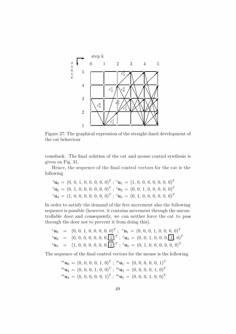
8/7/2019 Modelling and Control of Discrete Event Dynamic Systems
http://slidepdf.com/reader/full/modelling-and-control-of-discrete-event-dynamic-systems 51/61
b b b b b bb b b b b b
b b b b b bb b b b b bb b b b b b
e e e
e
e e e ¢
¢ ¢
¢ ¢ ¢ ¢ ¢ ¢ ¢ ¢
e e e e e e e
¡ ¡ ¡
¡ ¡ ¡ ¡ !e
e e e e e e
e e e e
e e e
g g g g g g g g g g g g g g
e e e e
e e e
¢ ¢ ¢
¢ ¢ ¢ ¢ ¢ ¢ ¢ ¢
g g g g g g g g g g g g g g
¡ ¡ ¡ ¡ ¡ ¡ ¡ !
e e e e e
e e ¡
¡ ¡ ¡ ¡
¡ ¡ !
c03
c14
c11
c28
c25
c22
c27
0
1
1 2 3 4 5
2
3
4
5
E step kcs
tate
Figure 27: The graphical expression of the straight-lined development of the cat behaviour
comeback. The final solution of the cat and mouse control synthesis isgiven on Fig. 31.
Hence, the sequence of the final control vectors for the cat is the
followingcu0 = (0, 0, 1, 0, 0, 0, 0, 0)T ; cu1 = (1, 0, 0, 0, 0, 0, 0, 0)T
cu2 = (0, 1, 0, 0, 0, 0, 0, 0)T ; cu3 = (0, 0, 1, 0, 0, 0, 0, 0)T
cu4 = (1, 0, 0, 0, 0, 0, 0, 0)T ; cu5 = (0, 1, 0, 0, 0, 0, 0, 0)T
In order to satisfy the demand of the free movement also the followingsequence is possible (however, it contains movement through the uncon-trollable door and consequently, we can neither force the cat to passthrough the door nor to prevent it from doing this).
cu0 = (0, 0, 1, 0, 0, 0, 0, 0)T ; cu1 = (0, 0, 0, 1, 0, 0, 0, 0)T
cu2 = (0, 0, 0, 0, 0, 0, 0, 1 )T ; cu3 = (0, 0, 1, 0, 0, 0, 1 , 0)T
cu4 = (1, 0, 0, 0, 0, 0, 0, 1 )T ; cu5 = (0, 1, 0, 0, 0, 0, 0, 0)T
The sequence of the final control vectors for the mouse is the following
mu0 = (0, 0, 0, 0, 1, 0)T ; mu1 = (0, 0, 0, 0, 0, 1)T
mu2 = (0, 0, 0, 1, 0, 0)T ; mu3 = (0, 0, 0, 0, 1, 0)T
mu4 = (0, 0, 0, 0, 0, 1)T ; mu5 = (0, 0, 0, 1, 0, 0)T
49
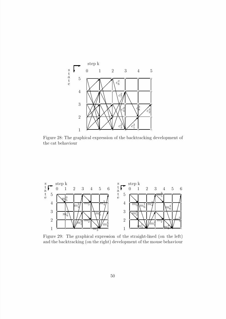
8/7/2019 Modelling and Control of Discrete Event Dynamic Systems
http://slidepdf.com/reader/full/modelling-and-control-of-discrete-event-dynamic-systems 52/61
b b b b b bb b b b b bb b b b b bb b b b b bb b b b b b
e e e e e e e
¢ ¢ ¢ ¢ ¢ ¢
¢ ¢ ¢ ¢ ¢
¡ ¡
¡ ¡ ¡ ¡ ¡ !
e
e e e e e e
g g g g g g g g
g g g g g g
g g g g g g g g
g g g g g g
e
e e e e e e
e e e e
e e e
e
e e e e
e e
g g g g g g g g
g g g g g g
e e e e e e e
¢ ¢ ¢ ¢ ¢ ¢
¢ ¢ ¢ ¢ ¢
¡ ¡
¡ ¡ ¡ ¡ ¡ !
c42
c38
c31
c26
c27
c24
c23
0
1
1 2 3 4 5
2
3
4
5
E step k
cstate
Figure 28: The graphical expression of the backtracking development of the cat behaviour
a a a a a a aa a a a a a a
a a a a a a aa a a a a a aa a a a a a ad
d d f f f f f f f x¡ ¡
¡ ¡ ¡ !
£ £
£ £ £ £ £ £ £ £ #
d d d
d d d
d d d
f f f f f f f x£ £
£ £ £ £ £ £ £ £ #
¡ ¡
¡ ¡ ¡ !
m05
m16
m24
m21
m35
m32
m43
m46
m54
m51
0
1
1 2 3 4 5 6
2
3
4
5
E step kc
state
a a a a a a aa a a a a a a
a a a a a a aa a a a a a aa a a a a a ad
d d
d d d
d d d
f f f f f f f x£ £
£ £ £ £ £ £ £ £ #
¡ ¡
¡ ¡ ¡ !d
d d
d d d
d d d
f f f f f f f x£ £
£ £ £ £ £ £ £ £ #
m02
m05
m13
m16
m21
m24
m32
m35
m43
m46
m54
0
1
1 2 3 4 5 6
2
3
4
5
E step kc
state
Figure 29: The graphical expression of the straight-lined (on the left)and the backtracking (on the right) development of the mouse behaviour
50
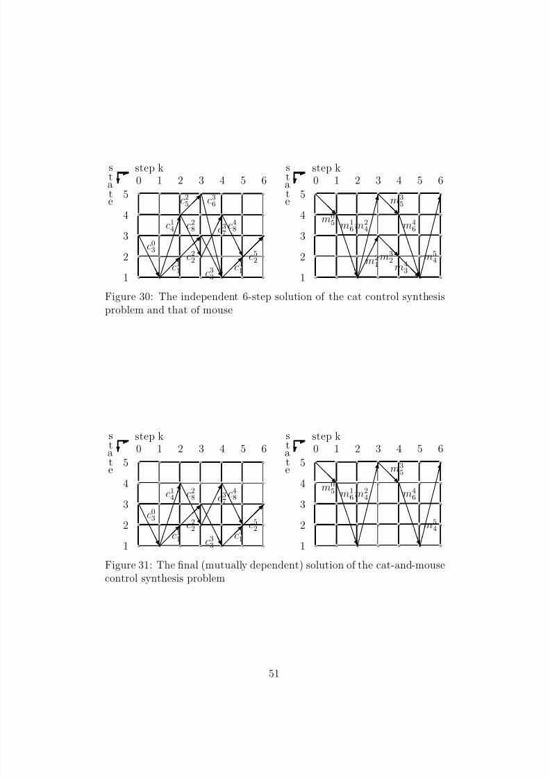
8/7/2019 Modelling and Control of Discrete Event Dynamic Systems
http://slidepdf.com/reader/full/modelling-and-control-of-discrete-event-dynamic-systems 53/61
a a a a a a aa a a a a a aa a a a a a aa a a a a a aa a a a a a a
e e e
e e
e e e
e e
c33 c
4
1
c52
¢ ¢ ¢ ¢ ¢ ¢ ¢ e
e e e e ¡
¡ ¡ ¡ ¡ !e
e e e e
c14 c28 c37c48
c03
c
1
1
c22
g
g g g g g g g
g g
c25 c36
0
1
1 2 3 4 5 6
2
3
4
5
E step kc
state
a a a a a a aa a a a a a aa a a a a a aa a a a a a aa a a a a a a
£ £ £ £ £ £ £ £ £ £ #
¡ ¡ ¡ ¡ ¡ !
f f f f f f f x
d d d
d d d
d d d
d
d d
f f f f f f f x£
£ £ £ £ £ £ £ £ £ #
m32
m
4
3
m54
m16m2
4 m46
m05
m21
m35
0
1
1 2 3 4 5 6
2
3
4
5
E step kc
state
Figure 30: The independent 6-step solution of the cat control synthesisproblem and that of mouse
a a a a a a aa a a a a a aa a a a a a aa a a a a a aa a a a a a a
e e e e
e
e e e e
e
c3
3
c41c52
¢
¢ ¢ ¢ ¢ ¢ ¢ e
e e e e ¡
¡ ¡ ¡ ¡ !e
e e e e
c14 c28 c37c48
c03
c11c22
0
1
1 2 3 4 5 6
2
3
4
5
E step kc
state
a a a a a a aa a a a a a aa a a a a a aa a a a a a aa a a a a a a
£
£ £ £ £ £ £ £ £ £ #
f f f f f f
f x
d d d
d d d
f f f f f f
f x£
£ £ £ £ £ £ £ £ £ #
m54
m16m2
4 m46
m05
m35
0
1
1 2 3 4 5 6
2
3
4
5
E step kc
state
Figure 31: The final (mutually dependent) solution of the cat-and-mousecontrol synthesis problem
51
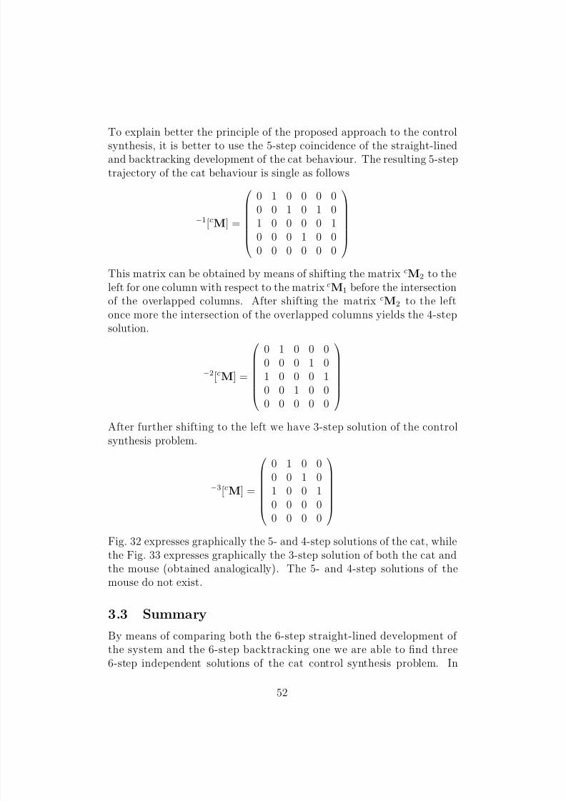
8/7/2019 Modelling and Control of Discrete Event Dynamic Systems
http://slidepdf.com/reader/full/modelling-and-control-of-discrete-event-dynamic-systems 54/61
To explain better the principle of the proposed approach to the controlsynthesis, it is better to use the 5-step coincidence of the straight-linedand backtracking development of the cat behaviour. The resulting 5-steptrajectory of the cat behaviour is single as follows
−1[cM] =
0 1 0 0 0 00 0 1 0 1 01 0 0 0 0 10 0 0 1 0 00 0 0 0 0 0
This matrix can be obtained by means of shifting the matrix cM2
to theleft for one column with respect to the matrix cM1 before the intersectionof the overlapped columns. After shifting the matrix cM2 to the leftonce more the intersection of the overlapped columns yields the 4-stepsolution.
−2[cM] =
0 1 0 0 00 0 0 1 01 0 0 0 10 0 1 0 00 0 0 0 0
After further shifting to the left we have 3-step solution of the controlsynthesis problem.
−3[cM] =
0 1 0 00 0 1 01 0 0 10 0 0 00 0 0 0
Fig. 32 expresses graphically the 5- and 4-step solutions of the cat, whilethe Fig. 33 expresses graphically the 3-step solution of both the cat andthe mouse (obtained analogically). The 5- and 4-step solutions of themouse do not exist.
3.3 Summary
By means of comparing both the 6-step straight-lined development of the system and the 6-step backtracking one we are able to find three6-step independent solutions of the cat control synthesis problem. In
52
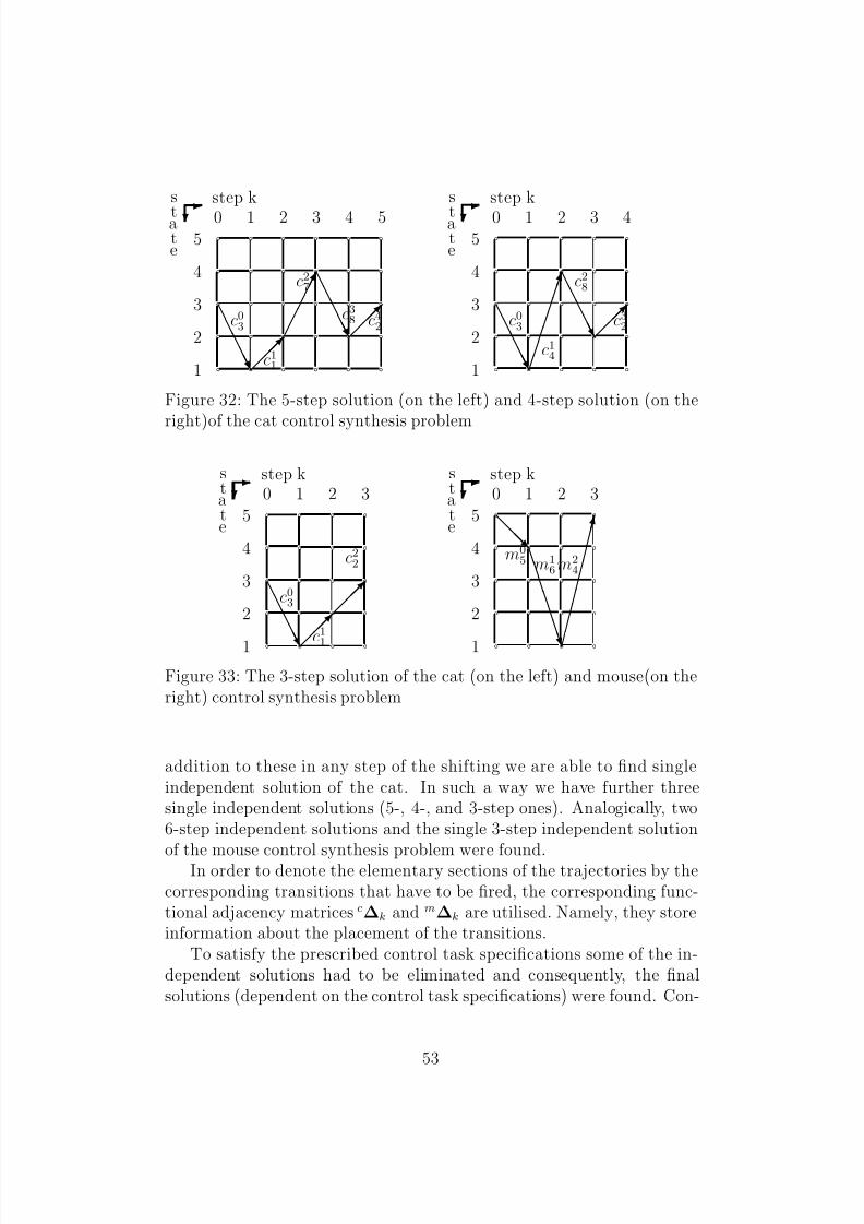
8/7/2019 Modelling and Control of Discrete Event Dynamic Systems
http://slidepdf.com/reader/full/modelling-and-control-of-discrete-event-dynamic-systems 55/61
a a a a a aa a a a a aa a a a a aa a a a a aa a a a a a
e e e e e ¡
¡ ¡ ¡ ¡ !
e e e e e
c03
c11
c42c38
c27
0
1
1 2 3 4 5
2
3
4
5
E step k
c
s
tate
a a a a aa a a a aa a a a aa a a a aa a a a a
e e e e e
¢ ¢ ¢ ¢ ¢ ¢ ¢
e e e e e
c03
c14
c32
c28
0
1
1 2 3 4
2
3
4
5
E step k
c
s
tate
Figure 32: The 5-step solution (on the left) and 4-step solution (on the
right)of the cat control synthesis problem
a a a aa a a aa a a aa a a aa a a a
e e e e e
c03
c1
1
c22
0
1
1 2 3
2
3
4
5
E step kc
state
a a a aa a a aa a a aa a a aa a a a
£
£ £ £ £ £ £ £ £ £ #
f f f f f f
f x
d d d
m16m2
4m0
5
0
1
1 2 3
2
3
4
5
E step kc
state
Figure 33: The 3-step solution of the cat (on the left) and mouse(on theright) control synthesis problem
addition to these in any step of the shifting we are able to find singleindependent solution of the cat. In such a way we have further threesingle independent solutions (5-, 4-, and 3-step ones). Analogically, two6-step independent solutions and the single 3-step independent solution
of the mouse control synthesis problem were found.In order to denote the elementary sections of the trajectories by thecorresponding transitions that have to be fired, the corresponding func-tional adjacency matrices c∆k and m∆k are utilised. Namely, they storeinformation about the placement of the transitions.
To satisfy the prescribed control task specifications some of the in-dependent solutions had to be eliminated and consequently, the finalsolutions (dependent on the control task specifications) were found. Con-
53

8/7/2019 Modelling and Control of Discrete Event Dynamic Systems
http://slidepdf.com/reader/full/modelling-and-control-of-discrete-event-dynamic-systems 56/61
sequently, we have to compare the 6-step solution of the cat and that of the mouse and confront them with the control task specifications. Thesame can be done with the 3-step solutions. Hence, the 6-step solutionof the cat-and-mouse problem given on Fig. 31 can be understood to bemore complex like the 3-step solution given on Fig. 33. In addition tothis we can see that the mouse solution is periodical with the periodequal to 3 steps.
The main aim of the dissection of the cat-and-mouse problem solvinginto details was the endeavour to demonstrate the applicability of theproposed approach. Although the control task specifications were givenonly verbally, the approach makes possible to solve the control synthesis
problem in analytical terms. However, if we want to solve the problemfully automatically knowledge about the control task specifications hasto be represent in appropriate form. It is very important at the choice of the most suitable solution.
4 Conclusions
The problem of modelling and control of DEDS was solved in this report.The determining priority was the endeavour to find such models andcontrol synthesis procedures that can be expressed in analytical terms.Two main kinds of the analytical models were presented - the PN-basedmodels and the OG-based ones. While the PN-based models are suitablefor the class of DEDS that can be described by OPN, the OG-basedmodels are suitable only for state machines (i.e. special kind of PN).Both of the kinds of models were utilised at the analytical approaches toDEDS control synthesis.
Because the control task specifications are usually given verbally or inanother non-analytical form, the suitable rule-based knowledge represen-tation was used in order to quantify them. LPN and FPN were used onthis way. Resulting KB was utilised in the proposed PN-based approach.
The graphical tools for the DEDS modelling, for the KB creation, andeven for the automatic knowledge-based control synthesis of DEDS weredeveloped and described.
Several illustrative examples were solved in order to demonstrate theliveness of the proposed approaches.
54

8/7/2019 Modelling and Control of Discrete Event Dynamic Systems
http://slidepdf.com/reader/full/modelling-and-control-of-discrete-event-dynamic-systems 57/61
Acknowledgement
I should like to thanks Prof. Mogens Nielsen, director of BRICS, forcreating very good conditions for my work. My thanks belong also toDr. Uffe Engberg for his help at solving practical problems connectedwith finalisation of this report. Finally, I thank also to Mrs. JanneChristensen for the efficient administrative help.
References
[1] Zoltan Bugar. Logical Petri nets and fuzzy Petri nets as the meansof knowledge representation (in Slovak). Master Thesis (Supervisor:Capkovic, F.). Department of Informatics, Faculty of Mathemat-ics and Physics, Comenius University, Bratislava, Slovak Republic.1998.
[2] Frantisek Capkovic. A Petri nets-based approach to the maze prob-lem solving . In Discrete Event Systems: Modelling and Control . (S.Balemi, P. Kozak and R. Smedinga, editors). Birkhauser Verlag,Basel - Boston - Berlin. 1993. 173–179.
[3] FrantisekˇCapkovic. Knowledge-based control of DEDS . In Proc. of the 13th IFAC World Congress 1996, San Francisco, USA, June 30-
July 5, 1996 (J.J. Gertler, J.B. Cruz and M. Peshkin, editors). Vol.J. Elsevier Science Ltd., Pergamon. paper J-3c-02.6. 1996. 347–352.also on Compact Disc.
[4] Frantisek Capkovic. Petri nets and oriented graphs in fuzzy knowl-edge representation for DEDS control purposes. BUSEFAL. 69,1997. 21–30.
[5] Frantisek Capkovic. Fuzzy knowledge in DEDS control synthesis.
In Proc. of the 7th International Fuzzy Systems Association World Congress - IFSA’97, Prague, Czech Republic, June 25-29, 1997 . (M.Mares, R. Mesiar, V. Novak, J. Ramık, A. Stupnanova, editors).Academia, Prague, Czech Republic. 1997. 550–554.
[6] Frantisek Capkovic. An approach to knowledge-representation at control of DEDS . In Advances in Intelligent Systems (F.C. Mora-bito, editor). IOS Press, Ohmsha, Amsterdam-Berlin-Oxford-Tokyo-Washington DC. 1997. 458–463.
55

8/7/2019 Modelling and Control of Discrete Event Dynamic Systems
http://slidepdf.com/reader/full/modelling-and-control-of-discrete-event-dynamic-systems 58/61
[7] Frantisek Capkovic. Representation of fuzzy knowledge about con-trol task specifications. In IT & KNOWS Information Technologiesand Knowledge Systems. Proceedings of XV. IFIP World Computer Congress, August 31-September 4, 1998, Vienna, Austria, and Bu-dapest Hungary . (J. Cuena, editor). Riegelnik, Vienna. 1998. 215–228. also on Compact Disc.
[8] Frantisek Capkovic. Knowledge-based control synthesis of discreteevent dynamic systems. In Advances in Manufacturing Systems.Decision, Control and Information Technology ( S.G. Tzafestas,editor). Chapter 19. Springer Verlag, London. 1998. 195–206.
[9] Frantisek Capkovic. Knowledge-based control of production systems.In Proc. of the 6th European Congress on Intelligent Techniques & Computing - EUFIT’98, September 7-10, 1998, Aachen, Germany .(H.J. Zimmermann, editor). ELITE Foundation, Aachen. Vol. 3.1998. 1565-1569.
[10] Frantisek Capkovic. Fuzzy knowledge in control of manufacturing systems. BUSEFAL. 75, 1998. 4–17.
[11] Frantisek Capkovic. Automated solving of the DEDS control prob-
lems. In Multiple Approaches to Intelligent Systems (I. Imam, Y. Ko-dratoff, A. El-Dessouki and M. Ali, editors). Lecture Notes in Arti-ficial Intelligence. Springer, Berlin-Heidelberg-New York-Barcelona-Hong Kong-London-Milan-Paris-Singapore-Tokyo. Vol. 1611. 1999.735–746.
[12] Peter Capkovic. Algorithm of the DEDS control synthesis and its program realization (in Slovak). Master Thesis (Supervisor:Capkovic, F.). Department of Informatics, Faculty of Electrical En-gineering and Information Technology, Slovak University of Tech-nology, Bratislava, Slovak Republic. 1999.
[13] Peter Capkovic. Algorithm of the DEDS control synthesis and itsprogram realization. User Handbook (in Slovak). Department of In-formatics, Faculty of Electrical Engineering and Information Tech-nology, Slovak University of Technology, Bratislava, Slovak Repub-lic. 1999.
[14] D.Y. Chao, M. C. Zhou and D.T. Wang. The knitting technique and Petri nets synthesis. The Computer Journal. 37, 1994. 67-76.
56

8/7/2019 Modelling and Control of Discrete Event Dynamic Systems
http://slidepdf.com/reader/full/modelling-and-control-of-discrete-event-dynamic-systems 59/61
[15] S.M. Chen, J.S. Ke and J.F. Chang. Knowledge representation us-ing fuzzy Petri nets. IEEE Transactions on Knowledge and DataEngineering. 2 No 3, 1990 311-319.
[16] Marian Csontos. Timed and time Petri nets in modelling discreteevent dynamic systems (in Slovak). Master Thesis (Supervisor:Capkovic, F.). Department of Informatics, Faculty of Mathemat-ics and Physics, Comenius University, Bratislava, Slovak Republic.2000.
[17] M. Diaz and P. Senac. The stream Petri nets: A model for timed multimedia information . In Proceedings of the 15th International Conference on Application and Theory of Petri Nets 1994, Zaragoza,Spain (R. Valette, editor). Lecture Notes in Computer Science. Vol.815. Springer. 1994. 219-238.
[18] F. DiCesare, G. Harhalakis, J.M. Proth, M. Silva and F.B. Vernadat.Practice of Petri nets in Manufacturing . Chapman & Hall. 1993.
[19] R. Diestel. Graph Theory Springer-Verlag, New York. 1997.
[20] M. Fiedler. Special Matrices and their Using in Numerical Mathe-matics (in Czech). SNTL Publishing House, Prague, Czechoslovakia.
1981.
[21] S. Kirkland, D.D. Olesky, and P. van den Driessche. Digraphs with large exponent . The Electronics Journal of Linear Algebra. 7. 2000.30–40.
[22] C.G. Looney, A.A., Alfize. Logical controls via boolean rule matrix transformations. IEEE Trans. on Syst. Man and Cybern. SMC-17.No 6. 1987. 1077–1081.
[23] C.G. Looney. Fuzzy Petri nets for rule-based decision-making . IEEE
Trans. Syst. Man Cybern. SMC-18. No 1. 1988. 178–183.
[24] Csaba Nemes. Graphical editor for the Petri nets creation (in Slo-vak). Master Thesis (Supervisor: Capkovic, F.). Department of Informatics, Faculty of Mathematics and Physics, Comenius Uni-versity, Bratislava, Slovak Republic. 1997.
[25] J.L. Peterson. Petri Net Theory and Modeling the Systems. PrenticeHall, New York. 1981.
57

8/7/2019 Modelling and Control of Discrete Event Dynamic Systems
http://slidepdf.com/reader/full/modelling-and-control-of-discrete-event-dynamic-systems 60/61
[26] J. Plesnık. Graph Algorithms (in Slovak). VEDA. Bratislava,Czechoslovakia. 1983.
[27] F.P. Preparata, R.T. Yeh. Introduction to Discrete Structures.Addison-Wesley Publ. Comp., Reading, USA. 1974.
[28] J. Sedlacek. Introduction to Graph Theory (in Czech). Academia,Prague, Czechoslovakia. 1977.
[29] S.G. Tzafestas, F. Capkovic. Petri net-based approach to synthesis of intelligent control for DEDS In Computer Assisted Management and Control of Manufacturing Systems (S.G. Tzafestas, editor). Chapter
12. Springer Verlag, Berlin-Heidelberg-New York. 1996. 325–351.
[30] H. Wielandt. Indecomposable non-negative matrices (in German).Math. Zeitschrift. 52. 1950. 642–648.
[31] W.M. Wonham, P.J. Ramadge. On the supremal controllable sub-language of a given language. SIAM J. Control and Optimization.25. 1987. 637–659.
58

8/7/2019 Modelling and Control of Discrete Event Dynamic Systems
http://slidepdf.com/reader/full/modelling-and-control-of-discrete-event-dynamic-systems 61/61
Recent BRICS Report Series Publications
RS-00-26 Frantisek Capkovic. Modelling and Control of Discrete Event
Dynamic Systems. October 2000. 58 pp.
RS-00-25 Zoltan Esik. Continuous Additive Algebras and Injective Simu-
lations of Synchronization Trees. September 2000. 41 pp.
RS-00-24 Claus Brabrand and Michael I. Schwartzbach. Growing Lan-
guages with Metamorphic Syntax Macros. September 2000.
RS-00-23 Luca Aceto, Anna Ingolfsdottir, Mikkel Lykke Pedersen, and
Jan Poulsen. Characteristic Formulae for Timed Automata.September 2000. 23 pp.
RS-00-22 Thomas S. Hune and Anders B. Sandholm. Using Automata
in Control Synthesis A Case Study. September 2000. 20 pp.
Appears in Maibaum, editor, Fundamental Approaches to Soft-
ware Engineering: First International Conference, FASE ’00
Proceedings, LNCS 1783, 2000, pages 349–362.
RS-00-21 M. Oliver Moller and Rajeev Alur. Heuristics for Hierarchical
Partitioning with Application to Model Checking. August 2000.
30 pp.
RS-00-20 Luca Aceto, Willem Jan Fokkink, and Anna Ingolfsdottir. 2-
Nested Simulation is not Finitely Equationally Axiomatizable.
August 2000. 13 pp.
RS-00-19 Vinodchandran N. Variyam. A Note on NP ∩ coNP/poly.
August 2000. 7 pp.
RS-00-18 Federico Crazzolara and Glynn Winskel. Language, Seman-
tics, and Methods for Cryptographic Protocols. August 2000.
ii+42 pp.
RS-00-17 Thomas S. Hune. Modeling a Language for Embedded Sys-
tems in Timed Automata. August 2000. 26 pp. Earlier version
entitled Modelling a Real-Time Language appeared in Gnesi
and Latella, editors, Fourth International ERCIM Workshop
on Formal Methods for Industrial Critical Systems, FMICS ’99
Proceedings of the FLoC Workshop, 1999, pages 259–282.