modelling and control of mechanical flexible systems · modelling and control of mechanical...
TRANSCRIPT
Modelling and Control of Mechanical
Flexible Systems
Doktor ingeniør dissertation
Mehrdad P. Fard
Report 2000:14-WDepartment of Engineering Cybernetics
Norwegian University of Science and TechnologyN-7034 Trondheim, NORWAY
2001
Abstract
This dissertation contains new results within the field of vibration control of flexiblemechanical systems. This work is focused on the vibration problems in slenderbodies. This due to the interest in studying active vibration damping of vortexinduced vibrations in marine risers.
Based on the original model of distributed-parameter systems, passivity propertiesof the underlying systems are proved. Simple feedback laws are derived to ensurethe stability of closed-loop and attenuation of vibration amplitude.
The control laws derived in this dissertation have require only measurements atthe top boundary of the beam. Hence, the effects of control and /or observationspillover are not an issue regarding to the stability or performance of the overallsystem. In addition, this method is cost efficient since it does not require severalmeasurement and actuators along the body.
Nonlinear model for transverse dynamics of a beam is derived. Based on thisnonlinear model, linear control laws are derived to ensure stability and convergentof the transverse deflection to zero. These control laws have very simple structureand are very simple to implement.
A coupled nonlinear model is derived, where both the longitudinal and transversedynamic of a beam are considered. Effect of longitudinal elongations on the trans-verse deflection is exploited to attenuate the transverse vibration of a beam. Thisis possible since by varying the strain, the tension along the beam is varied andhence the effective stiffness of the beam.
The main results of this dissertation have been published in international journalsand presented at international conferences. The most recent results are submittedfor publication in international journals and is currently under review.

ii
Acknowledgments
This thesis is submitted in partial fulfillment of the requirements for the degree ofdoctor engineer at the Norwegian University of Science and Technology (NTNU).The research work has been carried out partly at the Department of EngineeringCybernetics and partly at the Norsk Hydro’s Research Centre in Bergen duringthe period September 1997 to September 2000. The work has been funded by theNorwegian Research Council, under grant 119068/410, which I am grateful to.
I would like to thank my supervisor Professor Dr. Ing. Thor I. Fossen for super-vising my doctoral work and his encouragement to proceed this work.
I am also grateful to my research advisor Dr. Ing. Svein Ivar Sagatun for hisstrong involvement in this work. His valuable advises and comments during theresearch period have been a great help.
I would like to thank Professor Dr. Ing. Olav Egeland for his assistance in pro-viding fund for my doctoral study.
Special thank to my colleague Dr. Ing. Dag Kristiansen for valuable discussions.I also like to thank him and other colleagues at the Department of EngineeringCybernetics for creating a pleasant working environment.
I am also grateful to Norsk Hydro ASA for creating the opportunity to work inthe research center and the colleagues at the Marine Technology Department formaking my stay pleasant.
I will also thank my family who their continuous support has been a certainty andfor their encouragement to proceed my career.
Saving the best for the last, I would like to thank my dear son Arvin for being thegreatest source of inspiration and motivation and for giving meaning to my life.

iv
Nomenclature
Bold types are used to denote matrices and vectors. Bold uppercase denotesmatrices while lowercase denotes vectors.
XE, YE, ZE axes of inertial frameXB, YB, ZB axes of body frameXR, YR, ZR axes of riser frameXb, Yb, Zb axes of the coordinate frame at the bottom of seaRRB coordinate transformation matrix from body to riserRbR coordinate transformation matrix from riser to bottom of seaRbB coordinate transformation matrix from rody to bottom of seaL length of beam (riser), lagrangianq generalized coordinate vectorT kinetic energyV potential energyIy, Iz moments of inertia of riser about Y and Z directions, respectivelyA(x) cross-sectional area as a function of lengthD DiameterE Young’s modulusEA(x) axial stiffnessEI(x) bending stiffness, or flexural rigidityP (x, t) tensionP0 constant axial forcef(x, t) excitation force in Y -directionM MomentN axial-force-displacement relationu(t) control signaly(t) measurementCD drag coefficientCM mass coefficient
vi
Greek symbols
δ variational operatorε strainσ stressγ small positive constantγ1 small positive constantρ(x) mass density of riser per unit length as a function of lengthµ(x, t) displacement in longitudinal directionη(x, t) deflection in Y -directionφ, θ,ψ roll, pitch and yaw anglesφ(t, t0) transition function
Contents
Abstract i
Acknowledgements iii
Nomenclature vi
List of Figures xii
1 Introduction 1
1.1 Background . . . . . . . . . . . . . . . . . . . . . . . . . . . . . . . 1
1.2 Previous Works . . . . . . . . . . . . . . . . . . . . . . . . . . . . . 2
1.3 Contributions of this Thesis . . . . . . . . . . . . . . . . . . . . . . 4
1.4 Outline of the Thesis . . . . . . . . . . . . . . . . . . . . . . . . . . 4
2 Mathematical Modelling 7
2.1 Kinematics . . . . . . . . . . . . . . . . . . . . . . . . . . . . . . . 7
2.1.1 Transformation Matrix from Bottom to Riser, RRSB . . . . . 9
2.1.2 Transformation Matrix from Body to Riser, RRB . . . . . . . 10
2.1.3 Transformation Matrix from Body to Sea Bed, RSBB . . . . 10
2.2 Formulation of the Equations of Motion . . . . . . . . . . . . . . . 10
2.2.1 Newtonian Approach . . . . . . . . . . . . . . . . . . . . . . 11
2.2.2 The Principle of Virtual Work . . . . . . . . . . . . . . . . 11
2.2.3 Hamilton’s Principle . . . . . . . . . . . . . . . . . . . . . . 12
2.2.4 Lagrange’s Equation for Distributed Systems . . . . . . . . 12
2.3 Stress and Strain . . . . . . . . . . . . . . . . . . . . . . . . . . . . 14
2.3.1 Stress . . . . . . . . . . . . . . . . . . . . . . . . . . . . . . 14
viii CONTENTS
2.3.2 Strain . . . . . . . . . . . . . . . . . . . . . . . . . . . . . . 17
2.3.3 Hook’s Law . . . . . . . . . . . . . . . . . . . . . . . . . . . 20
2.4 Dynamic Equations of Motion for Beams in Bending . . . . . . . . 21
2.4.1 The Boundary-Value Problem for Beams in Bending . . . . 24
2.4.2 Transverse Dynamics of Beams in Bending . . . . . . . . . 28
2.5 Timoshenko Beam . . . . . . . . . . . . . . . . . . . . . . . . . . . 28
2.5.1 Justification for Euller-Bernoulli Beam . . . . . . . . . . . . 29
2.6 Effect of Axial Force on Transverse vibrations of Beams . . . . . . 31
2.7 Hydrodynamic Excitations . . . . . . . . . . . . . . . . . . . . . . . 32
2.7.1 Vortex Induced Vibration (VIV) . . . . . . . . . . . . . . . 32
2.7.2 Hydrodynamic Excitation Forces . . . . . . . . . . . . . . . 34
2.8 Marine Riser Systems . . . . . . . . . . . . . . . . . . . . . . . . . 35
2.8.1 Dynamic Model of Marine Risers . . . . . . . . . . . . . . . 36
2.8.2 Boundary Conditions . . . . . . . . . . . . . . . . . . . . . 38
2.8.3 Tensioners . . . . . . . . . . . . . . . . . . . . . . . . . . . . 38
2.9 Heave Compensation . . . . . . . . . . . . . . . . . . . . . . . . . . 42
2.9.1 Passive Heave Compensator . . . . . . . . . . . . . . . . . . 43
2.9.2 Active Heave Compensator . . . . . . . . . . . . . . . . . . 43
3 Passivity Analysis of Nonlinear Beams 47
3.1 Coupled Dynamic System . . . . . . . . . . . . . . . . . . . . . . . 48
3.2 Transverse Bending of a Beam . . . . . . . . . . . . . . . . . . . . 49
3.3 Transverse Bending of a Beam with Control Mechanism . . . . . . 51
3.4 Numerical Simulations . . . . . . . . . . . . . . . . . . . . . . . . . 53
3.4.1 Transversely Vibrating Beam . . . . . . . . . . . . . . . . . 54
3.4.2 Transversely Vibrating Beam with MDS Control Mechanism 54
3.5 Conclusions . . . . . . . . . . . . . . . . . . . . . . . . . . . . . . . 55
4 Boundary Control of a Transversely Vibrating Beam 61
4.1 Equations of Motion . . . . . . . . . . . . . . . . . . . . . . . . . . 61
4.1.1 Assumptions . . . . . . . . . . . . . . . . . . . . . . . . . . 62
4.2 Design of Boundary Control . . . . . . . . . . . . . . . . . . . . . . 62
4.2.1 Convergent Control Law . . . . . . . . . . . . . . . . . . . . 63
CONTENTS ix
4.2.2 Exponentially Stabilizing Control Law . . . . . . . . . . . . 65
4.3 External Disturbances . . . . . . . . . . . . . . . . . . . . . . . . . 69
4.4 Numerical Analysis . . . . . . . . . . . . . . . . . . . . . . . . . . . 72
4.4.1 Finite Difference Analysis . . . . . . . . . . . . . . . . . . . 73
4.4.2 Truncation Error . . . . . . . . . . . . . . . . . . . . . . . . 74
4.4.3 Consistency or Compatibility . . . . . . . . . . . . . . . . . 75
4.5 Numerical Simulation . . . . . . . . . . . . . . . . . . . . . . . . . 76
4.5.1 Convergent Control Law . . . . . . . . . . . . . . . . . . . . 76
4.5.2 Exponentially Stabilizing Control Law . . . . . . . . . . . . 77
4.6 Conclusions . . . . . . . . . . . . . . . . . . . . . . . . . . . . . . . 78
5 Boundary Control of a Coupled Nonlinear Beam 83
5.1 Equations of Motion . . . . . . . . . . . . . . . . . . . . . . . . . . 83
5.1.1 Assumptions . . . . . . . . . . . . . . . . . . . . . . . . . . 84
5.2 Design of Boundary Control Laws . . . . . . . . . . . . . . . . . . 84
5.2.1 Convergent Controller . . . . . . . . . . . . . . . . . . . . . 85
5.2.2 Exponentially Stabilizing Control Law . . . . . . . . . . . . 87
5.3 External Disturbances . . . . . . . . . . . . . . . . . . . . . . . . . 91
5.4 Conclusions . . . . . . . . . . . . . . . . . . . . . . . . . . . . . . . 92
6 Numerical Simulation of Coupled Dynamic 93
6.1 Nondimensional Formulation . . . . . . . . . . . . . . . . . . . . . 93
6.2 Discretization using Finite Difference Method . . . . . . . . . . . . 94
6.2.1 Truncation Error and Consistency . . . . . . . . . . . . . . 95
6.3 Numerical Analysis of the Control Law . . . . . . . . . . . . . . . . 96
6.3.1 Truncation Error and Consistency of the Control Law . . . 96
6.4 Numerical Simulation . . . . . . . . . . . . . . . . . . . . . . . . . 97
6.4.1 Convergent Control Law . . . . . . . . . . . . . . . . . . . . 98
6.4.2 Exponentially Stabilizing Control Law . . . . . . . . . . . . 98
6.5 Conclusions . . . . . . . . . . . . . . . . . . . . . . . . . . . . . . . 102
7 Conclusions 103
A Mathematical Preliminaries 111
x CONTENTS
A.1 Passivity . . . . . . . . . . . . . . . . . . . . . . . . . . . . . . . . . 111
A.2 Definitions and Theorems for Lyapunov Functionals . . . . . . . . 112
B Proof of Lemmas 117
B.1 Proof of Lemma 4.1 . . . . . . . . . . . . . . . . . . . . . . . . . . 117
B.2 Proof of Lemma 5.1 . . . . . . . . . . . . . . . . . . . . . . . . . . 119
List of Figures
2.1 Different reference frames. . . . . . . . . . . . . . . . . . . . . . . . 8
2.2 Traction force intensity on the boundary. . . . . . . . . . . . . . . 15
2.3 Traction forces on orthogonal faces. . . . . . . . . . . . . . . . . . . 16
2.4 Moment about an axis through the centre E and parallel to x3 axis. 17
2.5 Line segment in the undeformed geometry. . . . . . . . . . . . . . . 18
2.6 Line segment mapped to deformed geometry. . . . . . . . . . . . . 18
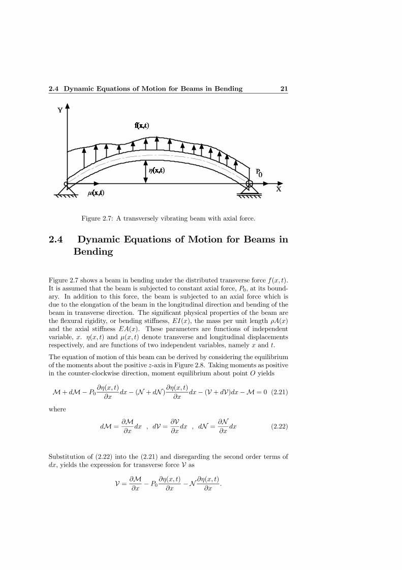
2.7 A transversely vibrating beam with axial force. . . . . . . . . . . . 21
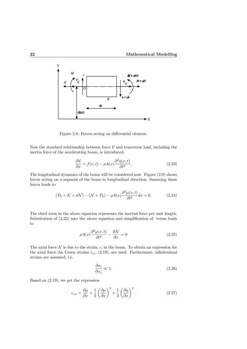
2.8 Forces acting on differential element. . . . . . . . . . . . . . . . . . 22
2.9 Forces acting on differential element. . . . . . . . . . . . . . . . . . 23
2.10 Rotation of vertical line segment. . . . . . . . . . . . . . . . . . . . 24
2.11 Timoshenko beam differential element. . . . . . . . . . . . . . . . . 29
2.12 Uniformly loaded beam. . . . . . . . . . . . . . . . . . . . . . . . . 29
2.13 A typical layout of riser system. . . . . . . . . . . . . . . . . . . . . 37
2.14 Marine riser system and associated equipments at boundaries. . . . 39
2.15 Sketch of top tension riser with buoyancy tanks. . . . . . . . . . . 41
2.16 Marine riser tensioners. . . . . . . . . . . . . . . . . . . . . . . . . 42
2.17 Top Mounted Drill String Compensator. . . . . . . . . . . . . . . . 43
2.18 Active heave compensation. . . . . . . . . . . . . . . . . . . . . . . 44
2.19 Active heave compensator’s cylinder stroke as a function of heavemotion. . . . . . . . . . . . . . . . . . . . . . . . . . . . . . . . . . 45
3.1 The closed-loop system. . . . . . . . . . . . . . . . . . . . . . . . . 49
3.2 A vibrating beam with a MDS boundary controller. . . . . . . . . 51
3.3 The closed-loop system. . . . . . . . . . . . . . . . . . . . . . . . . 53
xii LIST OF FIGURES
3.4 Transverse responses at differnet nodes, when only the first modeof vibration is excited. . . . . . . . . . . . . . . . . . . . . . . . . . 55
3.5 Total energy content of the riser. . . . . . . . . . . . . . . . . . . . 56
3.6 Transverse displacement at different nodes, when several modes ofvibration are excited. . . . . . . . . . . . . . . . . . . . . . . . . . . 57
3.7 Comparison between control forces. . . . . . . . . . . . . . . . . . . 57
3.8 Comparison between controlled and uncontrolled responses of theriser, when only the first mode of vibration is excited. . . . . . . . 58
3.9 Energy content of the system with MDS control mechanism. . . . . 58
3.10 Comparison between control forces. . . . . . . . . . . . . . . . . . . 59
3.11 Comparison between controlled and uncontrolled responses of theriser, when several modes of vibration are excited. . . . . . . . . . 59
4.1 Comparison between forced and free vibration responses, when firstmode is excited. . . . . . . . . . . . . . . . . . . . . . . . . . . . . . 77
4.2 Controller outputs with only first mode being excited. . . . . . . . 78
4.3 Comparison of transverse responses of the riser at different nodes,when several modes of vibration are excited. . . . . . . . . . . . . . 79
4.4 Comparison of the outputs of convergent controller with severalmodes being excited. . . . . . . . . . . . . . . . . . . . . . . . . . . 79
4.5 Comparison between forced and free vibration responses, when firstmode is excited. . . . . . . . . . . . . . . . . . . . . . . . . . . . . . 80
4.6 Comparison of exponentially stabilizing controller outputs with firstmode being excited. . . . . . . . . . . . . . . . . . . . . . . . . . . 80
4.7 The Lyapunov function V (t), (4.18). . . . . . . . . . . . . . . . . . 81
4.8 Comparison of transverse responses of the riser at different nodes,when several modes of vibration are excited. . . . . . . . . . . . . . 81
4.9 Comparison of exponentially stabilizing controller outputs with sev-eral modes being excited. . . . . . . . . . . . . . . . . . . . . . . . 82
6.1 Longitudinal and transverse responses of the riser. . . . . . . . . . 99
6.2 Control force u(t). . . . . . . . . . . . . . . . . . . . . . . . . . . . 99
6.3 Normalized mechanical energy. . . . . . . . . . . . . . . . . . . . . 100
6.4 Controlled and uncontrolled responses of the riser. . . . . . . . . . 100
6.5 Control force u(t). . . . . . . . . . . . . . . . . . . . . . . . . . . . 101
6.6 Normalized Lyapunov function. . . . . . . . . . . . . . . . . . . . . 101
Chapter 1
Introduction
1.1 Background
Vibration in slender bodies is a major problem in different engineering fields. Thesource of these vibrations and the nature of them might be different, like gallopingin transmission lines and vortex shedding vibrations in marine slender bodies. Amajor problem caused by vibrations in slender bodies is fatigue problem. Fatigueis a result of oscillating stresses in a material. Stress variation causes cracks todevelop and propagate from initial defects in the material. In general, the fatiguecapacity of a structure is given by the number of stress cycles before failure for agiven stress range.
In some engineering field, for instance oil and gas exploration, consequences offatigue problem in marine structures are more severe than in other fields. Manytypes of marine structures used in offshore industry, like pipe lines employed inoil exploration and production, tethers of TLP platforms, drilling and productionrisers, are exposed to vibrations caused by vortex shedding. These vibrationscauses wear and tear in structures like risers, with both environmental and financialconsequences. Fatigue damages in a marine riser can propagate and in a worstcase scenario cause severe environmental pollution. On the other hand, needs forinspection and repair reduce drilling productivity and cause shutdown of drillingoperations with obvious significant financial consequences.
This work is motivated by the industrial interests in stabilizing vibrating slen-der bodies. This is particularly an area of interest for the offshore engineeringcommunity. Increasing reliability and efficiency of operations, during drilling andexploration, in adverse sea environmental is a challenging research topic in off-shore engineering. Above mentioned problems become more and more significant,as offshore industry moves towards exploiting energy sources at deeper water.
2 Introduction
1.2 Previous Works
The motion of distributed-parameter structures is described by variables depend-ing on both time and space. As a result, the motion is governed by partial differ-ential equations to be satisfied inside a given domain defining the structure andby boundary conditions to be satisfied at points bounding this domain. Manyresearchers have devoted their works to modelling and analysis of the distributed-parameter systems. Modelling and analysis of this class of dynamic systems hasbeen covered extensively by many text books and papers. Meirovitch (1997) dis-cusses the modelling and analysis issues of continuous systems. In Nayfeh &Mook (1979) nonlinear vibrations and their stability issues of continuous systemsare studied. Modelling issues of cables are treated in Triantafyllou (1990). Sevin(1960) studied coupled dynamic of a column and the influence of axial inertia uponthe elastic bending motion of a column acted on by time dependent axial forces.
In essence, distributed-parameter systems presents problem not encountered inlumped-parameter systems, and many of the concepts are not applicable to distributed-parameter systems. The situation is different in using modal control, whichcorresponds to controlling a structure by controlling its modes. In this case,many of the concepts developed for lumped-parameter systems do carry over todistributed-parameter systems, since both types can be described in terms of modalcoordinates. The main difficulty arises in computing the control gains, as this im-plies infinite dimensional gain matrices. This question can be avoided by using theindependent modal-space control method, but this requires a distributed controlforce, which can be difficult to implement. One way to overcome this problem is toconstruct a truncated model consisting of a limited number of modes. In order todescribe the behavior of a flexible system in a satisfactory fashion, sometimes it isnecessary to include a large number of modes into the model. Thus, a characteris-tic of a truncated model is their large dimension. Hence, it becomes impractical tocontrol all modes. Therefore the control of such truncated systems are restricted toa few critical modes. This conversion into the finite dimensional model facilitatesapplication of control theory available for discrete systems. However, due to theignored high frequencies and uncertainties in design models, caused by truncationof the original model, PDE, the demands of high performance may not be satisfied.
Truncation of the infinite dimensional model divides the system into three modes:modelled controlled, modelled uncontrolled (residual) and unmodelled. In design-ing control system only the modelled modes are considered. In control problem ofsuch system the need for an observer arises from the fact that the system outputis in terms of the actual distributed system. Using observers in combination withtruncated models of distributed system leads to observation spillover. Controlsignal acting from actuators not only affects the controlled modes, as intended,but also influences the other modes, both residual and unmodelled. This is knownas control spillover, which is due to the fact that actuators are discrete. In Balas(1977), it is shown that the combined effect of control and observer spillover due tothe residual modes can destabilize the closed-loop system. However, in this paperthe residual modes are not included in the observer. It is shown in Meirovitch& Baruk (1983) that if the residual modes are included in the observer, no such
1.2 Previous Works 3
instability exists.
Boundary control is an efficient method to exclude the effect of both observa-tion and control spillover, since in this method the need for distributed actuatorsand sensors is omitted. In addition control design based on the original model,PDE, instead of an approximated discrete model improves the performance of asystem. In recent years, boundary control has received much attention amongcontrol researchers. Krabs & Leugering (1994) discusses boundary control of one-dimensional vibrating media whose motion is governed by a wave equation with a2n-order spatial self adjoint and positive definite linear differential operator. Baicu,Rahn & Nibali (1996) uses Hamilton’s principle to derive the governing nonlinearpartial differential equations of an elastic cable. Improved damping is achieved byboundary control. In Shahruz & Krishna (1996), Shahruz & Narasimha (1997)and Shahruz (1997) it is shown that feedback from the velocity at the boundaryof a string can stabilize the vibration in the string. In Fung, Wu & Wu (1999)asymptotic and exponential stability of an axially moving string is proven by us-ing a linear and nonlinear state feedback boundary control, respectively. It isproven that, in nonlinear feedback case, the mechanical energy of the system de-creases exponentially. In Fung & Tseng (1999) a boundary feedback state is usedto control the vibration of an axially moving string. The feedback state includesonly the displacement, velocity and slope at the right-hand side of the string. Inboth Fung et al. (1999) and Fung & Tseng (1999) the control laws are imple-mented via a mass-damper-spring at the right-hand side of the string. In Habib &Radcliffe (1991) controlled parameter fluctuation is used to reduce the structuralvibration of a nonlinear, simply supported Euler-Bernoulli beam through a bang-bang control law. Asymptotic stability of the system is proven via introducing aLyapunov’s functional. Coron & D’Andréa-Novel (1998) design a feedback torquecontrol law for a system consisting of a disk with a beam attached to its centerand perpendicular to the disk’s plane. The beam is confined to another planewhich is perpendicular to the disk and rotates with the disk. They prove that thefeedback control law ensures large asymptotic stability of the system when thereis no damping.
In robotics, the effects of link flexibility in robot manipulator systems have becomeimportant for researchers. Needs for lightweight robot systems have motivateddesign of flexible link robot arms. For example, space-based manipulators aremore likely to be characterized by long links manufactured from lightweight metalsor composites. Use of these links complicates the corresponding position controlproblem since the links are subject to deflection and vibration. Due to the problemsrelated to spillover effects and due to the ignorance of high frequency component ofthe system, boundary control strategies are preferable. Boundary control strategieshave been designed for flexible arms by several researchers, de Queiroz, Dawson,Agarwal & Zhang (1999), Luo (1993), Luo, Nobuyuki & Guo (1995). In Luo(1993) a control strategy called direct strain feedback (DSFB) is used to controlvibration of a flexible arm which is modelled as a beam. This control law introducesa damping into the governing equation and thus attenuate the vibration. Thesemigroup and operator theory are used to prove the stability of the system. InLuo et al. (1995) a control law consisting of feedback from shear force at the root
4 Introduction
end of an elastic arm is used to control the vibration of the arm. Exponentialstability of the closed loop system is proven.
Recently, boundary control has been applied in control of fluid flow and Burger’sequation, which arises in model studies of turbulence and shock wave theory, Krstic(1999), Balogh & Krstic (1999), Liu & Krstic (2000) and Balogh & Krstic (2000).
1.3 Contributions of this Thesis
• Nonlinear models: It is common to use linear Euler-Bernoulli beams haveto model marine risers. In order to simplify the analysis the coupling betweentransverse and longitudinal vibration is neglected. It is well known thattransverse and longitudinal vibrations of a beam are coupled, Nayfeh &Mook (1979), this dynamic coupling is taken into account in models derivedin this work. Since the oscillating stress is the major cause of fatigue problemit is important to take into account nonlinear oscillations in the model. UsingHamilton’s principle, the governing nonlinear partial differential equationsare derived.
• Analysis of passivity properties of nonlinear beams and passivitybased control laws: Passivity properties of three different nonlinear mod-els of beams are studied. A mass-damper-spring system is attached to thetop boundary of a transversely vibrating beam, which changes the losslesspassivity of the transverse vibrating beam to output-strictly passive. Basedon the passivity properties of the systems simple output feedbacks are de-signed. The resulting closed-loop systems are proven to be L2 stable. Thiswork has been presented in Fard & Sagatun (2000c).
• Convergent and exponentially stabilizing control laws for trans-versely vibrating nonlinear beams: Control laws have been derived fora nonlinear transversely vibrating beam based on its distributed-parametermodel. Stability analysis are carried out using Barbalats Lemma and Lya-punov’s stability theorems for distributed-parameter systems. An upperbound for total mechanical energy of the exponentially stabilized closed-loop system has been obtained for a class of distributed external distur-bances. Existence of this bound also indicates that the states of the systemare bounded in the presence of external disturbances. Part of this work hasbeen presented in Fard & Sagatun (2000a) and Fard & Sagatun (1999).
• Convergent and exponentially stabilizing control laws for couplednonlinear beams: Two controllers are derived for a nonlinear beam wherethe coupling between the longitudinal and transversal dynamics is incorpo-rated in the model. It is also proven that for a class of distributed distur-bance, an exponentially stabilized closed-loop system has an upper boundedtotal mechanical energy and an expression for this bound is derived. Hence,the boundedness of the states in the presence of external disturbances areproven. Part of this work has been presented in Fard & Sagatun (2000b).
1.4 Outline of the Thesis 5
1.4 Outline of the Thesis
The out line of this thesis is as follows:
• Chapter 2: Related topics to the dynamics of mechanical structures, suchas strain and stress, are reviewed in this chapter. Two nonlinear models forbeams in bending vibration are derived using Hamilton’s principle. A veryshort brief of vortex induced vibration is presented.
• Chapter 3: The passivity properties of the models derived in Chapter 2are studied. A control mechanism, consisting of a mass, a damper and aspring, is proposed which is attached to the top boundary of the transverselyvibrating beam. The passivity property of the combined system is studied.Furthermore, based on the passivity properties of each system, control lawsare suggested and the L2 stability properties of each closed-loop system isproven.
• Chapter 4: A control law using feedback from the velocity of a beam at thetop boundary is derived. Using Barbalats Lemma, it is proven that the statesof the system converge to equilibrium of the system. A simple linear controllaw using feedback from velocity and the slope of the top boundary of thebeam, is derived. Using this controller, exponential convergence of the statesof the closed-loop system is proved by Lyapunov’s method. Furthermore, itis proved that the total mechanical energy of the exponentially stabilizedclosed-loop system is upper bounded for a class of distributed disturbances.
• Chapter 5: In this chapter design of control laws are based on a nonlinearmodel of the beam where the coupling between the longitudinal and trans-verse dynamics of the beam is taken into the consideration. A control lawusing feedback from the longitudinal velocity at the top boundary is designedand convergence of the states of the closed-loop system is garanteed by Bar-balats Lemma. Another control law is derived which guarantees exponentialconvergence of the states of the closed-loop system. In addition, an expres-sion for the upper bound of the total mechanical energy of the exponentiallystabilized system, for a class of external disturbances, is derived.
• Chapter 6: Numerical analysis of coupled dynamic and control laws areperformed. Numerical simulations are carried out to test performance of theproposed control laws of the previous chapter. Simulation results from eachsimulations are compared.

6 Introduction
Chapter 2
Mathematical Modelling
Mathematical models of mechanical systems are divided into two broad classes:lumped parameter, or discrete models, and distributed parameter, or continuousmodels. Discrete systems consist of discrete components, such as springs andmasses. Masses are assumed to be rigid while springs being flexible but massless.The masses and the spring stiffnesses represent the system parameters, with themasses being concentrated at given points and connected by springs. In contrast,at each point of a continuous system there is both mass and stiffness, and theseparameters are distributed over the entire system. The position of a point in acontinuous system is identified by spatial coordinates. A set of all interior pointsdefines the domain of the system, while a set of points on the exterior of the domaindefines the boundary of the system. Since there is an infinite number of pointsin the domain, a distributed system is regarded as having an infinite number ofdegrees of freedom.
Mathematically, the motion of a discrete system with n-degree of freedoms is gov-erned by n simultaneous ordinary differential equations. In contrast, the motionof a distributed parameter system is governed by a set of partial differential equa-tions, which is valid over the domain of the system, and an appropriate numberof partial differential equations at every points of the boundary.
A continuous system can be approximated by a discrete model. The precision ofthe results can be made as refined as desired by increasing the number of degreesof freedom. But in principle an infinite number of degrees of freedom would berequired to converge to the exact results for any structure having distributed-parameter properties; Hence, using this approach to obtain an exact solution isimpossible.
2.1 Kinematics
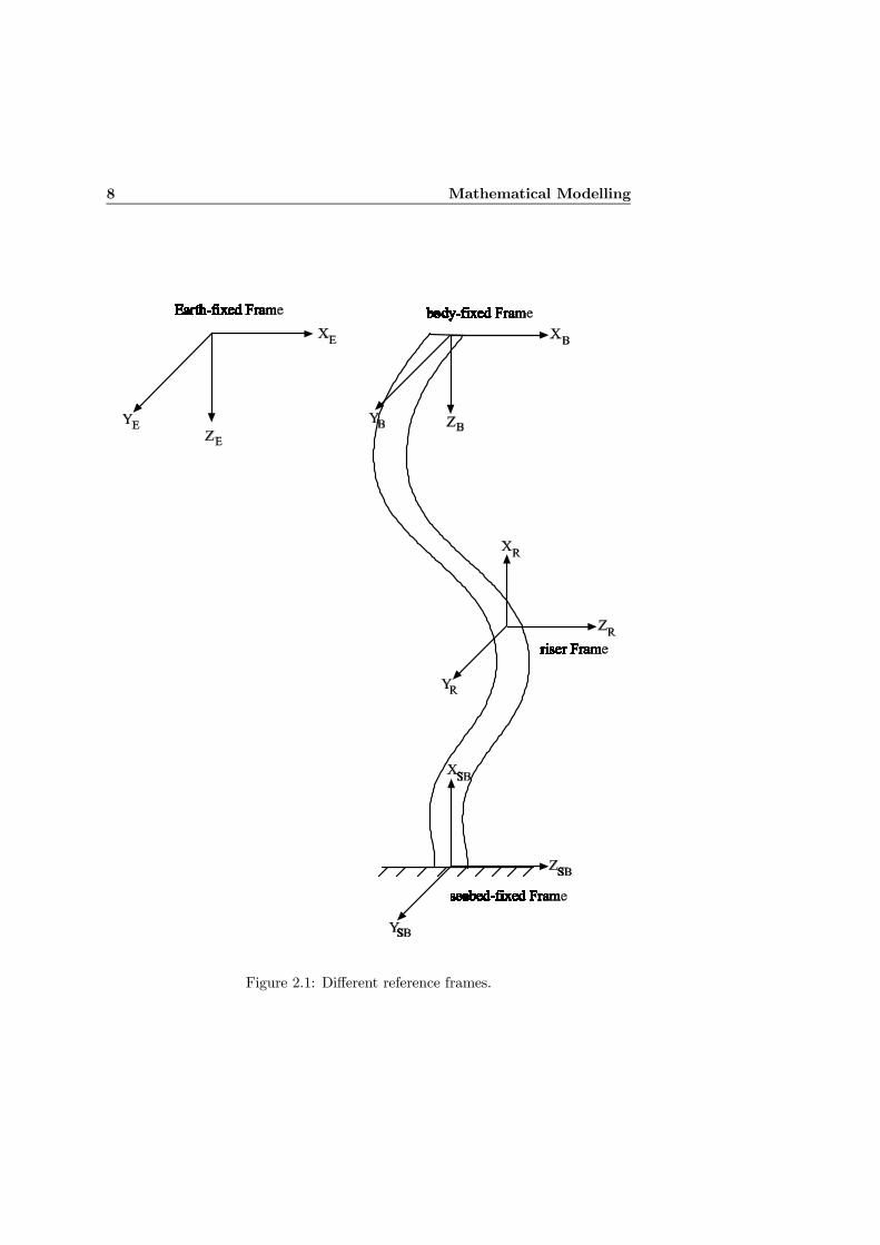
When studying marine risers it is convenient to introduce the following referenceframes, see Figure 2.1:
8 Mathematical Modelling
Figure 2.1: Different reference frames.
2.1 Kinematics 9
1. The Earth-fixed frame, denoted XEYEZE.
2. The body-fixed frame, denoted XBYBZB which is attached to the surfacevessel. The XBYB plane lies in the water surface, the ZB axis is positivedownwards.
3. The frame attached to the center line of the riser denoted XRYRZR withYRZR plane parallel to water surface and XR axis pointing from the bottomto the water surface, along the length of the riser.
4. The sea bed-fixed frame denoted XSBYSBZSB with YSBZSB plane layingon the sea floor and positive XSB axis pointing upwards from the sea floorto the water surface.
In deriving the transformation matrices for these frames we use the xyz-conventionspecified in terms of Euler angles for rotations, i.e. roll (φ), pitch (θ) and yaw (ψ).The basic rotation matrices representing rotations about X, Y and Z axes aregiven as
Rx,φ =
1 0 00 cosφ − sinφ0 sinφ cosφ
Ry,θ =
cos θ 0 sin θ0 1 0
− sin θ 0 cos θ
Rz,ψ =
cosψ − sinψ 0sinψ cosψ 00 0 1
2.1.1 Transformation Matrix from Bottom to Riser, RRSB
Let XRYRZR be obtained by translating the bottom-fixed coordinate system XSBYSBZSB parallel to itself until its origin coincides with origin of the riser frame.The coordinate system XRYRZR is rotated a yaw angle ψ about its ZR axis. Thecurrent axis is then rotated a pitch angle θ about its current Y 0R axis. The thirdrotation, a roll angle φ, is about the current X 00
R axis. The rotation sequence iswritten as
RRSB = Rz,ψRy,θRx,φ.
Using the basic rotation matrices we obtain
RRSB =
cψcθ −sψcφ+ cψsθsφ sψsφ+ cψsθcφsψcθ cψcφ+ sψsθsφ −cψsφ+ sψsθcφ−sθ cθsφ cθcφ
(2.1)
where s· = sin(·) and c· = cos(·). The notation Ri,α denotes a rotation angle αabout the i-axis.
10 Mathematical Modelling
2.1.2 Transformation Matrix from Body to Riser, RRB
The transformation matrix from body-fixed frame to the frame attached to theriser is obtained by the following basic rotations:
RRB =Rz,ψRy,θ+π
2Rx,φ.
Using the basic rotation matrixes and
Ry,θ+π2=
− sin θ 0 cos θ0 1 0
− cos θ 0 − sin θ
(2.2)
the transformation matrix RRB is obtained as
RRB =
−cψsθ −sψcφ+ cψcθsφ sψsφ+ cψcθcφ−sψsθ cψcφ+ sψcθsφ −cψsφ+ sψcθcφ−cθ −sθsφ −sθcφ
.
2.1.3 Transformation Matrix from Body to Sea Bed, RSBB
The transformation matrix from body-fixed frame to the sea bed coordinate systemis obtained by the following basic rotations about the current axes:
RSBB =Rz,ψRy,θ+π
2Rx,φ.
Using basic rotation matrices and rotation matrix in (2.2), the transformationmatrix RSB
B is given by
RSBB =
−cψsθ −sψcφ+ cψcθsφ sψsφ+ cψcθcφ−sψsθ cψcφ+ sψcθsφ −cψsφ+ sψcθcφ−cθ −sθsφ −sθcφ
.
All these transformation matrices belong to SO(3), which is the special orthogonalgroup of transformations in R3. Any rotation matrix, R, belonging to SO(3) isorthogonal, i.e. RT = R−1 =R, and has positive determinant, i.e. detR = 1.
2.2 Formulation of the Equations of Motion
Different methods can be utilized to derive the equations of motion of distributed-parameter dynamic systems, each having their advantages and characteristics. Thefundamental concepts of some methods will be shortly described in the followingparagraphs. The material in this section is mainly based on Clough & Penzien(1975), Meirovitch (1997) and Spong & Vidyasagar (1989).
2.2 Formulation of the Equations of Motion 11
2.2.1 Newtonian Approach
The equation of motion of any mechanical dynamic system represent expressionsof Newton’s second law of motion. This relationship can be expressed mathemat-ically as the differential equation
f(t) =d
dt
µmdr
dt
¶where f(t) is the applied force vector and r(t) is the position vector of the massm. For most problems in structural dynamics it may be assumed that the massdoes not vary with time. This expression may be written as
f(t)−md2r
dt2= 0.
The second term, md2rdt2 , is called inertia force and resist the acceleration of the
mass.
In Newtonian mechanics, motions are measured relative to an inertial referenceframe, i.e., a reference frame at rest or moving uniformly relative to an averageposition of fixed stars. This approach is a vectorial approach using physical co-ordinates to describe the motion. The force f(t) may be considered to includemany types of force acting on the mass such as elastic constraints which opposedisplacements, viscous forces which resist velocities, and independently defined ex-ternal loads. Thus if an inertia force which resists acceleration is introduced, theexpression of the equation of motion is merely an expression of the equilibrationof all of the forces acting on the mass.
2.2.2 The Principle of Virtual Work
The principle of virtual work is essentially a statement of static equilibrium ofa mechanical system. Before any further discussion, it is necessary to introducethe concept of virtual displacements. Assuming that the position of a point in aN dimensional space is given by ri(i = 1, 2, · · · , N), the virtual displacement isdefined as an imagined infinitesimal changes δri(i = 1, 2, · · · , N) in the positionwhich are consistent with the constraints of the system. The virtual displacementsare not true displacements but small variations in the system coordinates resultingfrom imagining the system in a slightly displaced position. In contrast to truedisplacement, this process does not involve any changes in time, so that the forcesand constraints do not change during this process.
The principle of virtual displacement can be expressed as follows. If a systemwhich is in equilibrium under the action of a set of forces is subjected to a virtualdisplacement, the total work performed by forces will be zero. Thus, the equationsof motion of a dynamic system can be established by introducing virtual displace-ments corresponding to each degree of freedom and equating the work done tozero, after identifying all forces acting on the system. In this approach the virtualwork distributions are scalar quantities, whereas the forces acting on the structuresare vectorial.
12 Mathematical Modelling
2.2.3 Hamilton’s Principle
This approach has the advantage that it is independent of the coordinates used incontrast with other approaches like Lagrangian. In addition, Hamilton’s principlepermits the derivation of equations of motion from scalar energy quantities in avariational form. This principle can be formulated as
Z t2
t1
δ(T − V +Wnc)dt = 0 (2.3)
where T is the kinetic energy, V the potential energy of the system including bothstrain and potential of any conservative external force. Wnc denotes work doneby nonconservative forces acting on system, including damping and any arbitraryexternal loads. The symbol δ indicates variation taken during indicated timeinterval.
This principle states that the variation of the potential and kinetic energy plusthe variation of work done by the nonconservative force during any time interval[t1, t2] must equal to zero. Application of this principle leads to the equation ofmotion for any given system. This approach enjoys the advantage of dealing solelywith scalar quantities such as kinetic and potential energies.
2.2.4 Lagrange’s Equation for Distributed Systems
For most mechanical systems, discrete systems, the potential energy can be ex-pressed in terms of the generalized coordinates, q = (q1,q2, ..., qn)T , while thekinetic energy can be expressed in terms of the generalized coordinate vector, q,and its first time derivative. In addition the virtual work which is performed bynonconservative forces as they act through the virtual displacements caused byarbitrary set of variations in the generalized coordinates can be expressed as alinear function of those variations. Once these scalar functions are expressed interms of generalized coordinates, the well-known Lagrange’s equation,
∂
∂t
µ∂T
∂qi
¶− ∂T
∂qi+
∂V
∂qi= Qi i = 1, · · · , n (2.4)
can readily be derived from the Hamilton’s principle, (2.31). Q1, Q2, ..., Qn arethe generalized forces corresponding to the coordinates q1,q2, ..., qn.
However, the situation is more complicated in the case of distributed systems,because there are at least two independent variables instead of one. In addition,the potential energy of the distributed systems is usually a function of not onlythe generalized coordinates alone but also the spatial derivatives of those as well.
For distributed systems, kinetic and potential energies, in terms of generalized
2.2 Formulation of the Equations of Motion 13
coordinates, can be written as
T =
Z L
0
T (q)dx (2.5)
V =
Z L
0
V (q,q0,q00) (2.6)
where T and V are kinetic and potential energy intensities, respectively. Moreover,the virtual work is simply
δWnc =
Z L
0
f(x, t)δqdx (2.7)
where f(x, t) is a vector of generalized forces corresponding to generalized coor-dinate, q. Notice that concentrated forces can be expressed as distributed bymeans of spatial Dirac delta functions. The extended Hamilton’s principle, (2.31),requires variation of the Lagrangian L = T − V .
δL =
Z L
0
δLdx =
Z L
0
̶L
∂qδq+
∂L
∂q0δq0+
∂L
∂q00δq00 +
∂L
∂qδq
!dx
We need to carry out integration by parts with respect to x and t. First, we carryout the integration with respect to t,Z t2
t1
∂L
∂qδqdt =
∂L
∂qδq
¯¯t2
t1
−Z t2
t1
∂
∂t
̶L
∂q
!δqdt = −
Z t2
t1
∂
∂t
̶L
∂q
!δqdt (2.8)
Note that the fact that δq is zero at t = t1, t2 is used here. Next step is to carryout integration by parts with respect to x. It is assumed that differentiation andvariation are interchangeable; Hence,Z L
0
∂L
∂q0δq0dx =
Z L
0
∂L
∂q0∂
∂xδqdx =
∂L
∂q0δq
¯¯L
0
−Z L
0
∂
∂x
̶L
∂q0
!δqdx. (2.9)
Similarly,Z L
0
∂L
∂q00δq00 =
∂L
∂q00δq0¯¯L
0
− ∂
∂x
̶L
∂q00
!δq
¯¯L
0
+
Z L
0
∂2
∂x2
̶L
∂q00
!δqdx (2.10)
Introducing (2.7)-(2.10) into the (2.31) yields
Z t2
t1
∂L
∂q0δq
¯¯L
0
+∂L
∂q00δq0¯¯L
0
− ∂
∂x
̶L
∂q00
!δq
¯¯L
0
+
Z L
0
"∂L
∂q− ∂
∂x
̶L
∂q0
!+
∂2
∂x2
̶L
∂q00
!− ∂
∂t
̶L
∂q
!+ f(x, t)
#δqdx
)dt = 0.
(2.11)
14 Mathematical Modelling
At this point, the arbitrariness of the virtual displacement is invoked. We letδq(0, t) = δq(L, t) = 0 and δq0(0, t) = δq0(L, t) = 0, and conclude that (2.11) issatisfied for all values of δq with x ∈ (0, L) if and only if
∂L
∂q− ∂
∂x
̶L
∂q0
!+
∂2
∂x2
̶L
∂q00
!− ∂
∂t
̶L
∂q
!+ f(x, t) = 0 (2.12)
for ∀ (x, t) ∈ (0, L)× [0,∞). Boundary conditions may be derived from
∂L
∂q0δq
¯¯L
0
+∂L
∂q00δq0¯¯L
0
− ∂
∂x
̶L
∂q00
!δq
¯¯L
0
= 0.
Boundary conditions are obtained by considering that either δq(0, t) or its coef-ficients are zero and either δq0(0, t) or its coefficient is zero. Similar statementscan be made about conditions at x = L. Equation (2.12) represents the Lagrangeequation of motion for distributed-parameter systems with lagrangian given byL = T − V , where T and V are as in (2.5)-(2.6).
It is worth noticing that the Lagrange equation, (2.12), was derived for systemswith Lagrangian given by (2.5)-(2.6). We did not consider possible sources ofpotential energy at the boundaries, as springs. In cases where such devices areattached to the boundaries, the potential energy due to these devices can be in-cluded to the expression for potential energy, (2.6). Inclusion of these terms willnot effect the Lagrange equation, (2.12), but changes the boundary conditions forthat particular system.
2.3 Stress and Strain
Material in this section is based on Shames & Dym (1985) and Ottosen & Petersson(1992). In the study of continuous media, we are concerned with the manner inwhich forces are transmitted through a medium. We are concerned with two classesof forces. The first is the so-called body force distribution (i.e. per unit volume),which is distinguished by the fact that it acts directly on the distribution of matterin the domain of specification. It is represented as a function of position and timeand denoted as b(x, y, z, t).
In discussing a continuum there may be some physical boundary that enclose thedomain of interest, such as the outer surface of a beam, or we may elect to specifya domain and thereby generate a ”mathematical” boundary. In either case, wewill be concerned with the force distribution that is applied to such boundariesdirectly from material outside the domain of interest. Such force distributions arecalled surface tractions (i.e. per unit area) and denoted by t(x, y, z, t).
2.3.1 Stress
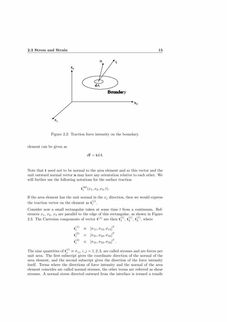
Consider a surface of body, as shown in Figure 2.2, over which we have a surfacetraction distribution t at some time t. The force df transmitted across this area
2.3 Stress and Strain 15
Figure 2.2: Traction force intensity on the boundary.
element can be given as
df = tdA.
Note that t need not to be normal to the area element and so this vector and theunit outward normal vector n may have any orientation relative to each other. Wewill further use the following notations for the surface traction
t(n)i (x1, x2, x3, t).
If the area element has the unit normal in the xj direction, then we would expressthe traction vector on the element as t(j)i .
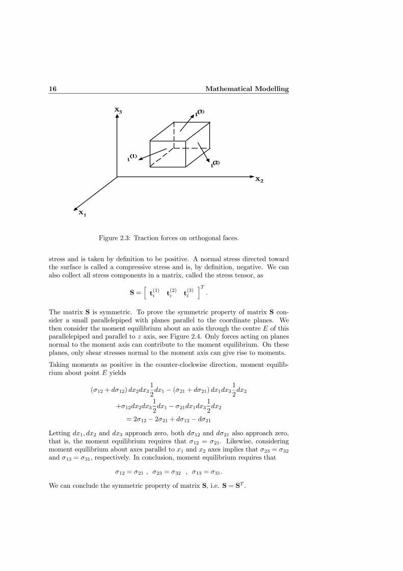
Consider now a small rectangular taken at some time t from a continuum. Ref-erences x1, x2, x3 are parallel to the edge of this rectangular, as shown in Figure2.3. The Cartesian components of vector t(1) are then t(1)1 , t
(1)2 , t
(1)3 , where
t(1)i ≡ [σ11,σ12,σ13]
T
t(2)i ≡ [σ21,σ22,σ23]
T
t(3)i ≡ [σ31,σ32,σ33]
T .
The nine quantities of t(i)j ≡ σij , i, j = 1, 2, 3, are called stresses and are forces perunit area. The first subscript gives the coordinate direction of the normal of thearea element, and the second subscript gives the direction of the force intensityitself. Terms where the directions of force intensity and the normal of the areaelement coincides are called normal stresses, the other terms are referred as shearstresses. A normal stress directed outward from the interface is termed a tensile
16 Mathematical Modelling
Figure 2.3: Traction forces on orthogonal faces.
stress and is taken by definition to be positive. A normal stress directed towardthe surface is called a compressive stress and is, by definition, negative. We canalso collect all stress components in a matrix, called the stress tensor, as
S =ht(1)i t
(2)i t
(3)i
iT.
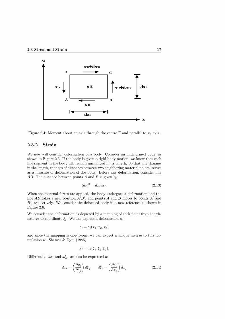
The matrix S is symmetric. To prove the symmetric property of matrix S con-sider a small parallelepiped with planes parallel to the coordinate planes. Wethen consider the moment equilibrium about an axis through the centre E of thisparallelepiped and parallel to z axis, see Figure 2.4. Only forces acting on planesnormal to the moment axis can contribute to the moment equilibrium. On theseplanes, only shear stresses normal to the moment axis can give rise to moments.
Taking moments as positive in the counter-clockwise direction, moment equilib-rium about point E yields
(σ12 + dσ12) dx2dx31
2dx1 − (σ21 + dσ21) dx1dx3 1
2dx2
+σ12dx2dx31
2dx1 − σ21dx1dx3
1
2dx2
= 2σ12 − 2σ21 + dσ12 − dσ21Letting dx1, dx2 and dx3 approach zero, both dσ12 and dσ21 also approach zero,that is, the moment equilibrium requires that σ12 = σ21. Likewise, consideringmoment equilibrium about axes parallel to x1 and x2 axes implies that σ23 = σ32and σ13 = σ31, respectively. In conclusion, moment equilibrium requires that
σ12 = σ21 , σ23 = σ32 , σ13 = σ31.
We can conclude the symmetric property of matrix S, i.e. S = ST .
2.3 Stress and Strain 17
Figure 2.4: Moment about an axis through the centre E and parallel to x3 axis.
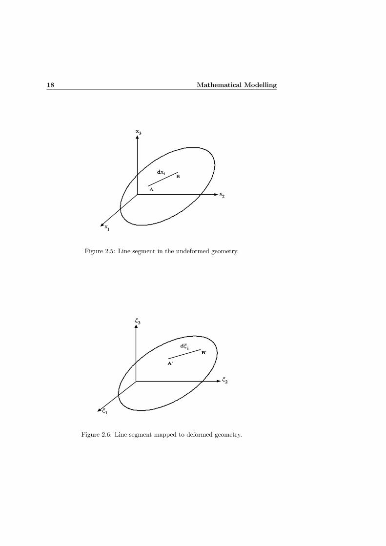
2.3.2 Strain
We now will consider deformation of a body. Consider an undeformed body, asshown in Figure 2.5. If the body is given a rigid body motion, we know that eachline segment in the body will remain unchanged in its length. So that any changesin the length, changes of distances between two neighboring material points, servesas a measure of deformation of the body. Before any deformation, consider lineAB. The distance between points A and B is given by
(ds)2 = dxidxi. (2.13)
When the external forces are applied, the body undergoes a deformation and theline AB takes a new position A0B0, and points A and B moves to points A0 andB0, respectively. We consider the deformed body in a new reference as shown inFigure 2.6.
We consider the deformation as depicted by a mapping of each point from coordi-nate xi to coordinate ξi. We can express a deformation as
ξi = ξi(x1, x2, x3)
and since the mapping is one-to-one, we can expect a unique inverse to this for-mulation as, Shames & Dym (1985)
xi = xi(ξ1, ξ2, ξ3).
Differentials dxi and dξi can also be expressed as
dxi =
µ∂xi∂ξj
¶dξj dξi =
µ∂ξi∂xj
¶dxj (2.14)
18 Mathematical Modelling
Figure 2.5: Line segment in the undeformed geometry.
Figure 2.6: Line segment mapped to deformed geometry.
2.3 Stress and Strain 19
We can now express the length (ds)2 in (2.13) as
(ds)2 = dxidxi =∂xi∂ξm
∂xi∂ξk
dξmdξk. (2.15)
In deformed state we have
(ds0)2 = dξidξi =∂ξi∂xk
∂ξi∂xl
dxkdxl. (2.16)
We now can find the change in length of the segment, by using both formulations,(2.15) and (2.16).
(ds0)2 − (ds)2 =µ∂ξk∂xi
∂ξk∂xj
dxidxj − ∂xk∂ξi
∂xk∂ξj
dξidξj
¶=
µ∂ξk∂xi
∂ξk∂xj
dxidxj − ∂xk∂ξi
∂xk∂ξj
µ∂ξi∂xj
¶dxj
µ∂ξj∂xi
¶dxi
¶=
µ∂ξk∂xi
∂ξk∂xj
dxidxj − ∂xk∂xj
∂xk∂xi
dxidxj
¶=
µ∂ξk∂xi
∂ξk∂xj− ∂xk
∂xj
∂xk∂xi
¶dxidxj
In a similar way we can obtain
(ds0)2 − (ds)2 =µ∂ξk∂ξi
∂ξk∂ξj− ∂xk
∂ξi
∂xk∂ξj
¶dξidξj
We now introduce the strain terms as
²ij =1
2
µ∂ξk∂xi
∂ξk∂xj− ∂xk
∂xj
∂xk∂xi
¶(2.17)
ηij =1
2
µ∂ξk∂ξi
∂ξk∂ξj− ∂xk
∂ξi
∂xk∂ξj
¶(2.18)
The set of terms ²ij in (2.17) is called Green’s strains. They are expressed asfunctions of the coordinates in the undeformed state and indicate what must occurduring a given deformation. The set of terms ηij in (2.18) is formulated as afunction of the coordinate for the deformed state. They indicate what must haveoccurred to reach the new geometry from an earlier undeformed state.
We now define the displacement field ui = ξi − xi which gives the displacementof each point in the body from the undeformed configuration to the deformedconfiguration. We obtain the following relations
∂xi∂ξj
=∂ξi∂ξj− ∂ui
∂ξj∂ξi∂xj
=∂ui∂xj
+∂xi∂xj
20 Mathematical Modelling
Substitution of these into (2.17) and (2.18) we obtain
²ij =1
2
µ∂ui∂xj
+∂uj∂xi
+∂uk∂xi
∂uk∂xj
¶(2.19)
ηij =1
2
µ∂ui∂ξj
+∂uj∂ξi
+∂uk∂ξi
∂uk∂ξj
¶(2.20)
2.3.3 Hook’s Law
Stresses and strains are related to each other. These relations are dependent onthe nature of the material under consideration and are called constitutive laws.We will assume linear elastic behavior where each stress component is linearlyrelated, in general to all strains. In on dimension, linear elasticity is expressed byHook’s law
σ = E²
where the material constant E is Young’s modulus. However, for several stressand strain components this relation is expressed by Hook’s generalized law as
σ = D²
where D is a 6× 6 matrix and
σ =£σ11 σ22 σ33 σ12 σ13 σ23
¤T² =
£²11 ²22 ²33 ²12 ²13 ²23
¤T.
Symmetric property of D matrix is an established property, see Ottosen & Peters-son (1992), Shames & Dym (1985) and references therein. Due to this symmetrythe 36 elements of the D matrix reduces to 21.
Generally, the D-matrix changes if another coordinate system is chosen. Isotropyproperty of mechanical behavior of a body require that mechanical properties ofthe body are not dependent on direction. Isotropy property requires that D-matrix is the same for all coordinate systems. For isotropic material we have
D =E
(1 + v) (1− 2v)
1− v v v 0 0 0v 1− v v 0 0 0v v 1− v 0 0 00 0 0 1
2 (1− 2v) 0 00 0 0 0 1
2 (1− 2v) 00 0 0 0 0 1
2 (1− 2v)
where we have to independent coefficients, Young’s modulus and Poisson’s ratiov.
2.4 Dynamic Equations of Motion for Beams in Bending 21
Figure 2.7: A transversely vibrating beam with axial force.
2.4 Dynamic Equations of Motion for Beams inBending
Figure 2.7 shows a beam in bending under the distributed transverse force f(x, t).It is assumed that the beam is subjected to constant axial force, P0, at its bound-ary. In addition to this force, the beam is subjected to an axial force which isdue to the elongation of the beam in the longitudinal direction and bending of thebeam in transverse direction. The significant physical properties of the beam arethe flexural rigidity, or bending stiffness, EI(x), the mass per unit length ρA(x)and the axial stiffness EA(x). These parameters are functions of independentvariable, x. η(x, t) and µ(x, t) denote transverse and longitudinal displacementsrespectively, and are functions of two independent variables, namely x and t.
The equation of motion of this beam can be derived by considering the equilibriumof the moments about the positive z-axis in Figure 2.8. Taking moments as positivein the counter-clockwise direction, moment equilibrium about point O yields
M+ dM− P0 ∂η(x, t)∂x
dx− (N + dN )∂η(x, t)∂x
dx− (V + dV)dx−M = 0 (2.21)
where
dM =∂M∂x
dx , dV = ∂V∂xdx , dN =
∂N∂xdx (2.22)
Substitution of (2.22) into the (2.21) and disregarding the second order terms ofdx, yields the expression for transverse force V as
V = ∂M∂x− P0 ∂η(x, t)
∂x−N ∂η(x, t)
∂x.
22 Mathematical Modelling
Figure 2.8: Forces acting on differential element.
Now the standard relationship between force V and transverse load, including theinertia force of the accelerating beam, is introduced.
∂V∂x
= f(x, t)− ρA(x)∂2η(x, t)
∂t2. (2.23)
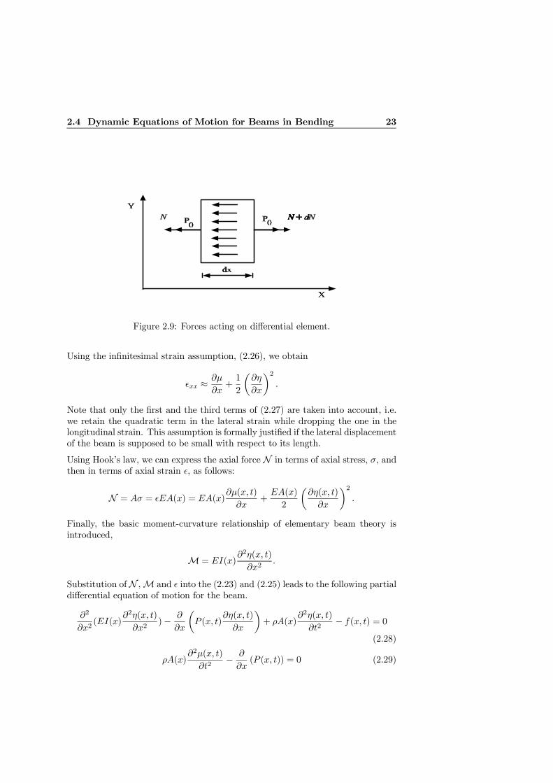
The longitudinal dynamics of the beam will be considered now. Figure (2.9) showsforces acting on a segment of the beam in longitudinal direction. Summing theseforces leads to
(P0 +N + dN )− (N + P0)− ρA(x)∂2µ(x, t)
∂t2dx = 0. (2.24)
The third term in the above equation represents the inertial force per unit length.Substitution of (2.22) into the above equation and simplification of terms leadsto
ρA(x)∂2µ(x, t)
∂t2− ∂N
∂x= 0 (2.25)
The axial force N is due to the strain, ², in the beam. To obtain an expression forthe axial force the Green strains εij , (2.19), are used. Furthermore, infinitesimalstrains are assumed, i.e.
∂ui∂xj
¿ 1. (2.26)
Based on (2.19), we get the expression
²xx =∂µ
∂x+1
2
µ∂µ
∂x
¶2+1
2
µ∂η
∂x
¶2. (2.27)
2.4 Dynamic Equations of Motion for Beams in Bending 23
Figure 2.9: Forces acting on differential element.
Using the infinitesimal strain assumption, (2.26), we obtain
²xx ≈ ∂µ
∂x+1
2
µ∂η
∂x
¶2.
Note that only the first and the third terms of (2.27) are taken into account, i.e.we retain the quadratic term in the lateral strain while dropping the one in thelongitudinal strain. This assumption is formally justified if the lateral displacementof the beam is supposed to be small with respect to its length.
Using Hook’s law, we can express the axial force N in terms of axial stress, σ, andthen in terms of axial strain ², as follows:
N = Aσ = ²EA(x) = EA(x)∂µ(x, t)
∂x+EA(x)
2
µ∂η(x, t)
∂x
¶2.
Finally, the basic moment-curvature relationship of elementary beam theory isintroduced,
M = EI(x)∂2η(x, t)
∂x2.
Substitution ofN ,M and ² into the (2.23) and (2.25) leads to the following partialdifferential equation of motion for the beam.
∂2
∂x2(EI(x)
∂2η(x, t)
∂x2)− ∂
∂x
µP (x, t)
∂η(x, t)
∂x
¶+ ρA(x)
∂2η(x, t)
∂t2− f(x, t) = 0
(2.28)
ρA(x)∂2µ(x, t)
∂t2− ∂
∂x(P (x, t)) = 0 (2.29)
24 Mathematical Modelling
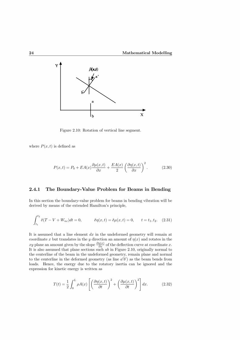
Figure 2.10: Rotation of vertical line segment.
where P (x, t) is defined as
P (x, t) = P0 +EA(x)∂µ(x, t)
∂x+EA(x)
2
µ∂η(x, t)
∂x
¶2. (2.30)
2.4.1 The Boundary-Value Problem for Beams in Bending
In this section the boundary-value problem for beams in bending vibration will bederived by means of the extended Hamilton’s principle,
Z t2
t1
δ(T − V +Wnc)dt = 0, δη(x, t) = δµ(x, t) = 0, t = t1, t2. (2.31)
It is assumed that a line element dx in the undeformed geometry will remain atcoordinate x but translates in the y direction an amount of η(x) and rotates in thexy plane an amount given by the slope ∂η(x)
∂x of the deflection curve at coordinate x.It is also assumed that plane sections such ab in Figure 2.10, originally normal tothe centerline of the beam in the undeformed geometry, remain plane and normalto the centerline in the deformed geometry (as line a0b0) as the beam bends fromloads. Hence, the energy due to the rotatory inertia can be ignored and theexpression for kinetic energy is written as
T (t) =1
2
Z L
0
ρA(x)
"µ∂η(x, t)
∂t
¶2+
µ∂µ(x, t)
∂t
¶2#dx. (2.32)
2.4 Dynamic Equations of Motion for Beams in Bending 25
The expression for the potential energy can be written as
V (t) =1
2
Z L
0
"EI(x)
µ∂2η(x, t)
∂x2
¶2+ P0
µ∂η(x, t)
∂x
¶2
+ EA(x)
Ã∂µ(x, t)
∂x+1
2
µ∂η(x, t)
∂x
¶2!2dx. (2.33)
This expression consists of three parts. The first term is due to the bending,second term is due to the axial force and third term is the strain energy of thebeam. It should be noted that if the axial force P0 in the second term in (2.33)varied with position along the beam (for example, considering the weight of thebeam) it would be necessary to modify (2.33) only by including the axial forceexpression under the integral sign.
Finally, the virtual work done by nonconservative forces can be expressed by
δWnc =
Z L
0
f(x, t)δη(x, t)dx. (2.34)
It is assumed that the variations and differentiations are interchangeable and theoperations involved in (2.31) will be carried out. We start with the expression forkinetic energy, (2.32). For the sake of simplicity the argument (x, t) is omittedand the variation in the kinetic energy is written as
δT (t) = ρA
Z L
0
·∂η
∂tδ∂η
∂t+
∂µ
∂tδ∂µ
∂t
¸dx
= ρA
Z L
0
·∂η
∂t
∂
∂tδη +
∂µ
∂t
∂
∂tδµ
¸dx.
Integrating by parts, we obtain
δT (t) = ρA
Z t2
t1
Z L
0
·∂η
∂t
∂
∂tδη +
∂µ
∂t
∂
∂tδµ
¸dxdt
= ρA
Z L
0
Z t2
t1
·∂η
∂t
∂
∂tδη +
∂µ
∂t
∂
∂tδµ
¸dtdx
= ρA
Z L
0
"∂η
∂tδη
¯t2t1
+∂µ
∂tδµ
¯t2t1
#dx
−ρAZ L
0
Z t2
t1
·∂2η
∂t2δη +
∂2µ
∂t2δµ
¸dtdx
= −ρAZ t2
t1
Z L
0
·∂2η
∂t2δη +
∂2µ
∂t2δµ
¸dxdt (2.35)
where the fact that δη = δµ = 0 at t = t1, t2.

26 Mathematical Modelling
Furthermore, the variation of potential energy, (2.33), is given as
δV (t) =
Z L
0
"EI
∂2η
∂x2δ∂2η
∂x2+ P0
∂η
∂xδ∂η
∂x+1
2EA
µ∂η
∂x
¶2δ∂µ
∂x
+EA∂µ
∂x
∂η
∂xδ∂η
∂x+1
2EA
µ∂η
∂x
¶3δ∂η
∂x+EA
∂µ
∂xδ∂µ
∂x
#dx. (2.36)
Changing the variations and differentiations and carrying out integration by partsfor each terms in (2.36) yields
δV (t) = EI∂2η
∂x2∂
∂xδη
¯L0
− ∂
∂x
µEI
∂2η
∂x2
¶δη
¯L0
+ P0∂η
∂xδη
¯L0
+1
2EA
µ∂η
∂x
¶2δµ
¯¯L
0
+ EA∂µ
∂x
∂η
∂xδη
¯L0
+1
2EA
µ∂η
∂x
¶3δη
¯¯L
0
+ EA∂µ
∂xδµ
¯L0
+
Z L
0
∂2
∂x2
µEI
∂2η
∂x2
¶δηdx− P0
Z L
0
∂2η
∂x2δηdx− 1
2
Z L
0
∂
∂x
ÃEA
µ∂η
∂x
¶2!δµdx
−Z L
0
∂
∂x
µEA
∂µ
∂x
∂η
∂x
¶δηdx− 1
2
Z L
0
∂
∂x
ÃEA
µ∂η
∂x
¶3!δηdx
−Z L
0
∂
∂x
µEA
∂µ
∂x
¶δµdx (2.37)
Finally, inserting (2.34), (2.35) and (2.37) into (2.31) and collecting terms in ap-propriate groups, we obtainZ t2
t1
Z L
0
·½µ−ρA∂
2η
∂t2
¶− ∂2
∂x2
µEI
∂2η
∂x2
¶+
∂
∂x
µEA
∂µ
∂x
∂η
∂x
¶+P0
∂2η
∂x2+1
2
∂
∂x
ÃEA
µ∂η
∂x
¶3!+ f
)δηdx
+
Z L
0
(−ρA∂
2µ
∂t2+
∂
∂x
µEA
∂µ
∂x
¶+1
2
∂
∂x
ÃEA
µ∂η
∂x
¶2!)δµdx
− EI ∂2η
∂x2δ∂η
∂x
¯L0
+
½∂
∂x
µEI
∂2η
∂x2
¶− P0 ∂η
∂x
−EA∂µ∂x
∂η
∂x− 12EA
µ∂η
∂x
¶3)δη
¯¯L
0
+
(−12EA
µ∂η
∂x
¶2−EA∂µ
∂x
)δµ
¯¯L
0
dt = 0 (2.38)
Now the arbitrariness of the virtual displacements is invoked. It is assumed thateither δη, δµ or theirs coefficients at the boundaries are zero, and either δ ∂η∂x or its
2.4 Dynamic Equations of Motion for Beams in Bending 27
coefficient at boundaries is zero. It is also assumed that δη and δµ are arbitraryover the domain 0 < x < L. Therefore, (2.38) can be satisfied if and only if
ρA∂2η(x, t)
∂t2+
∂2
∂x2
µEI
∂2η(x, t)
∂x2
¶− ∂
∂x
µEA
∂µ(x, t)
∂x
∂η(x, t)
∂x
¶−P0 ∂
2η(x, t)
∂x2− 12
∂
∂x
ÃEA
µ∂η(x, t)
∂x
¶3!− f(x, t) = 0 (2.39)
ρA∂2µ(x, t)
∂t2− ∂
∂x
µEA
∂µ(x, t)
∂x
¶− 12
∂
∂x
ÃEA
µ∂η(x, t)
∂x
¶2!= 0 (2.40)
∀ (x, t) ∈ (0, L)× [0,∞). In addition, either
− ∂
∂x
µEI
∂2η(x, t)
∂x2
¶+ P0
∂η(x, t)
∂x+EA
∂µ(x, t)
∂x
∂η(x, t)
∂x
+1
2EA
µ∂η(x, t)
∂x
¶3= 0 at x = 0, L (2.41)
or
η(x, t) = 0 at x = 0, L (2.42)
and either
EI∂2η(x, t)
∂x2= 0 at x = 0, L (2.43)
or
∂η(x, t)
∂x= 0 at x = 0, L (2.44)
and either
1
2EA
µ∂η(x, t)
∂x
¶2+EA
∂µ(x, t)
∂x= 0, at x = 0, L (2.45)
or
µ(x, t) = 0 at x = 0, L. (2.46)
Equations (2.39)-(2.40) represent the equations of motion. Equations (2.41)-(2.46)represent boundary conditions. Depending on the end support conditions twoof (2.41)-(2.44) and one of (2.45)-(2.46) must be satisfied. Geometric boundaryconditions, (2.42), (2.44) and (2.46) result from geometric compatibility, whilenatural boundary conditions, (2.41), (2.43) and (2.45) result from force balance.Boundary conditions (2.41) and (2.42) indicate that either shear force is zero or thetransversal displacement must be zero. Equations (2.43) and (2.44) requires thateither the bending moment or the slope of deflection must be zero. Finally (2.45)and (2.46) indicate that either the axial force or the longitudinal displacementmust be zero.
28 Mathematical Modelling
2.4.2 Transverse Dynamics of Beams in Bending
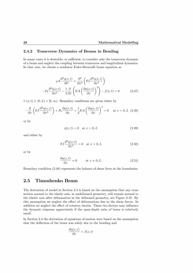
In many cases it is desirable, or sufficient, to consider only the transverse dynamicof a beam and neglect the coupling between transverse and longitudinal dynamics.In that case, we obtain a nonlinear Euler-Bernoulli beam equation as
ρA∂2η(x, t)
∂t2+
∂2
∂x2
µEI
∂2η(x, t)
∂x2
¶−P0 ∂
2η(x, t)
∂x2− 12
∂
∂x
ÃEA
µ∂η(x, t)
∂x
¶3!− f(x, t) = 0 (2.47)
∀ (x, t) ∈ (0, L)× [0,∞). Boundary conditions are given either by
− ∂
∂x
µEI
∂2η(x, t)
∂x2
¶+ P0
∂η(x, t)
∂x+1
2EA
µ∂η(x, t)
∂x
¶3= 0 at x = 0, L (2.48)
or by
η(x, t) = 0 at x = 0, L (2.49)
and either by
EI∂2η(x, t)
∂x2= 0 at x = 0, L (2.50)
or by
∂η(x, t)
∂x= 0 at x = 0, L. (2.51)
Boundary condition (2.48) represents the balance of shear force at the boundaries.
2.5 Timoshenko Beam
The derivation of model in Section 2.4 is based on the assumption that any crosssection normal to the elastic axis, in undeformed geometry, will remain normal tothe elastic axis after deformation in the deformed geometry, see Figure 2.10. Bythis assumption we neglect the effect of deformations due to the shear forces. Inaddition we neglect the effect of rotatory inertia. These two factors may influencethe dynamic response appreciately if the span-depth ratio of beam is relativelysmall.
In Section 2.4 the derivation of equations of motion were based on the assumptionthat the deflection of the beam was solely due to the bending and
∂η(x, t)
∂x= β(x, t)
2.5 Timoshenko Beam 29
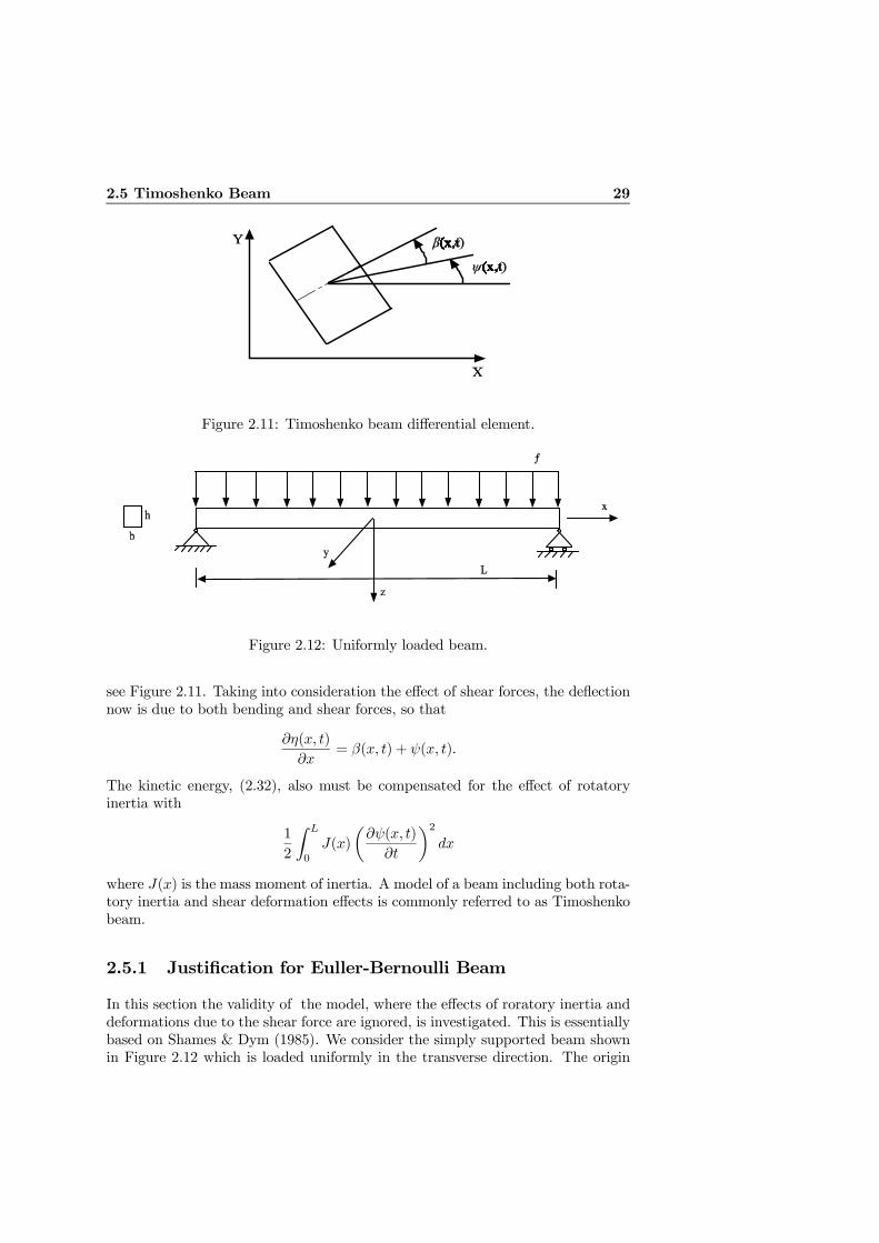
Figure 2.11: Timoshenko beam differential element.
Figure 2.12: Uniformly loaded beam.
see Figure 2.11. Taking into consideration the effect of shear forces, the deflectionnow is due to both bending and shear forces, so that
∂η(x, t)
∂x= β(x, t) + ψ(x, t).
The kinetic energy, (2.32), also must be compensated for the effect of rotatoryinertia with
1
2
Z L
0
J(x)
µ∂ψ(x, t)
∂t
¶2dx
where J(x) is the mass moment of inertia. A model of a beam including both rota-tory inertia and shear deformation effects is commonly referred to as Timoshenkobeam.
2.5.1 Justification for Euller-Bernoulli Beam
In this section the validity of the model, where the effects of roratory inertia anddeformations due to the shear force are ignored, is investigated. This is essentiallybased on Shames & Dym (1985). We consider the simply supported beam shownin Figure 2.12 which is loaded uniformly in the transverse direction. The origin
30 Mathematical Modelling
of reference is placed at the center of the beam. The boundary conditions usedfor this problem at x = ±L
2 are that both the deflection η(x, t) and the bending
momentM are zero. The latter is accomplished by requiring that ∂2η(x,t)∂x2 = 0 at
the ends.
The equation for the deflection of the center line may then be written as follows
∂4η(x, t)
∂x4=
f
EI.
Integrating four times we get
η(x, t) =fx4
24EI+C1
x3
6+C2
x2
2+C3x+C4.
Integration constants are determined from the boundary conditions
EI∂2η(x, t)
∂x2= 0 at x = ±L
2
η(x, t) = 0 at x = ±L2.
We then have for the deflection curve
η(x, t) =fL4
24EI
·³xL
´4− 32
³xL
´2+5
16
¸In developing this model we have neglected the shear strain energy. General ex-pression for strain energy is given by
Ustrin =1
2
Z Z ZV
τ ij²ijdv.
Denoting the shear strain energy as Ushear, we have
Ushear =1
2
Z Z ZV
τxz²xzdv =1
2G
Z Z ZV
τ2xzdv
where τxz = G²xz and, shear modulus, G = E2(1+ν) . Using
τxz = −dMdx
(1
2I)
µz2 − h
2
4
¶we obtain
Ushear =(1 + ν)
E
Z L2
−L2
Z h2
−h2
·fx
2I(z2 − h
2
4)
¸2bdzdx
=f2L5
240EI
"2(1 + ν)
µh
L
¶2#(2.52)
2.6 Effect of Axial Force on Transverse vibrations of Beams 31
We now compute the strain energy due to bending.
Ubend =EI
2
Z L2
−L2
µ∂2η(x, t)
∂x2
¶2dx =
f2L5
240EI(2.53)
Taking the ratio of (2.52) and (2.53) for comparison purposes, we obtain
UshearUbend
= 2(1 + ν)
µh
L
¶2Thus we see that the ratio of the shear strain energy to the bending strain energyis proportional to ( hL) squared. Hence, for long slender beams the shear strainenergy is very small compared to the bending strain energy and therefore it canbe neglected. On the contrary, for short stubby beams the contribution from shearstrain energy can not be neglected and must be taken into consideration.
2.6 Effect of Axial Force on Transverse vibrationsof Beams
When the coupling between the longitudinal and transverse dynamics is neglected,and it is assumed that the force P (x, t) = P0, is a tensile force, then (2.39) can bewritten as
ρA∂2η
∂t2+
∂2
∂x2
µEI
∂2η
∂x2
¶− P0 ∂
2η
∂x2− f(x, t) = 0. (2.54)
Boundary conditions, are zero deflection at boundaries,
η(x, t) = 0 at x = 0, L (2.55)
and , zero moment at boundaries,
EI∂2η(x, t)
∂x2= 0 at x = 0, L. (2.56)
Free vibration is assumed; hence, f(x, t) = 0 for t > t0. It is also assumed thatthe solution of (2.54) is separable in the spatial variable and time; hence, it hasthe form
η(x, t) =W (x)F (t). (2.57)
Introducing (2.57) into (2.54) we can write
ρAW (x)F (t) +EIF (t)∂4
∂x4W (x)− P0F (t) ∂
2
∂x2W (x) = 0 (2.58)
32 Mathematical Modelling
where it is assumed that the flexural rigidity is uniform along the length of thebeam, EI(x) = EI. Boundary conditions become
W (x) = 0 at x = 0, L
EI∂2
∂x2W (x) = 0 at x = 0, L.
Dividing through (2.58) by ρAW (x) we obtain
−1ρAW (x)
µEI
∂4
∂x4W (x)− P0 ∂2
∂x2W (x)
¶=
1
F (t)F (t). (2.59)
Since the right side of the above equation depends only on t and the left sidedepends only on x, the two sides of the equation must be equal to the sameconstant. This constant is denoted by −λ, where λ is positive. We set the left sideof (2.59) equal to −λ and obtain the differential equation
EI∂4
∂x4W (x)− P0 ∂2
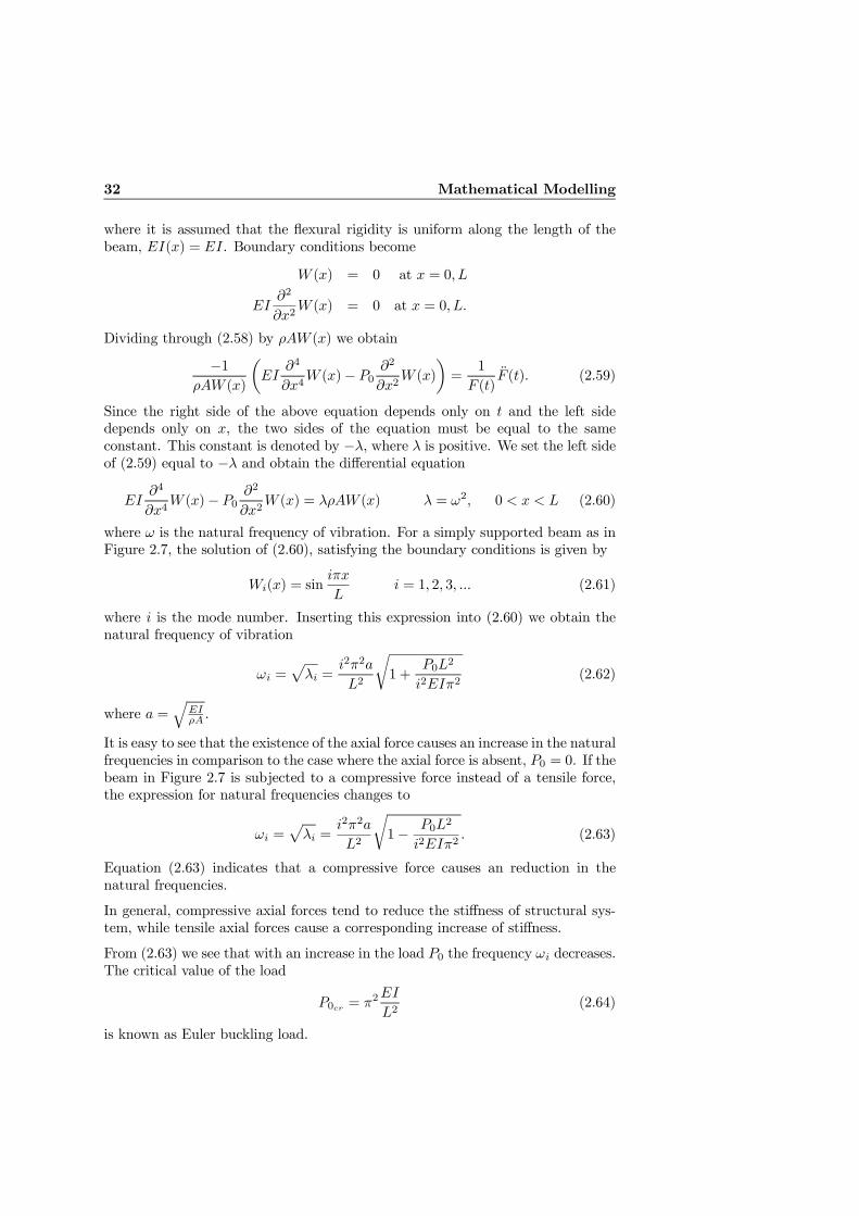
∂x2W (x) = λρAW (x) λ = ω2, 0 < x < L (2.60)
where ω is the natural frequency of vibration. For a simply supported beam as inFigure 2.7, the solution of (2.60), satisfying the boundary conditions is given by
Wi(x) = siniπx
Li = 1, 2, 3, ... (2.61)
where i is the mode number. Inserting this expression into (2.60) we obtain thenatural frequency of vibration
ωi =pλi =
i2π2a
L2
r1 +
P0L2
i2EIπ2(2.62)
where a =q
EIρA .
It is easy to see that the existence of the axial force causes an increase in the naturalfrequencies in comparison to the case where the axial force is absent, P0 = 0. If thebeam in Figure 2.7 is subjected to a compressive force instead of a tensile force,the expression for natural frequencies changes to
ωi =pλi =
i2π2a
L2
r1− P0L2
i2EIπ2. (2.63)
Equation (2.63) indicates that a compressive force causes an reduction in thenatural frequencies.
In general, compressive axial forces tend to reduce the stiffness of structural sys-tem, while tensile axial forces cause a corresponding increase of stiffness.
From (2.63) we see that with an increase in the load P0 the frequency ωi decreases.The critical value of the load
P0cr = π2EI
L2(2.64)
is known as Euler buckling load.
2.7 Hydrodynamic Excitations 33
2.7 Hydrodynamic Excitations
2.7.1 Vortex Induced Vibration (VIV)
The topic of vortex induced vibration has been subjected to many years of research.It is not the intention to carry out a profound discussion of this topic here, and justfor complementary sake we will briefly touch this topic in the following. Severaltext books have elaborated this topic, in addition many researches have reportedtheir works in this field. Among them we may refer to Griffin, Skop & Koopmann(1973), Griffin (1992), Griffin, Skop & Ramberg (1975), Griffin (1985) ,Vikestad(1998), Vandiver (1993), Larsen, Vandiver, Vikestad & Lie (n.d.), Faltinsen (1990)and references therein.
As a fluid flows by a circular cylinder, with diameter D, the pressure gradient isnegative up to a point where we obtain the lowest pressure on the body surface.On the downstream of this point the pressure increases and the velocity decreasesuntil separation point where the velocity gradient is zero. Flow separation occursat a point on the cylinder surface where a backflow in the boundary layer on thedownstream side of the point is encountered. When the process of flow separationstarts around the circular cylinder a symmetric wake picture develops. However,due to instabilities asymmetry will soon occur. The consequence is that vorticesare alternately shed from each side of the cylinder. It is observed that by varyingthe incident current velocity U , the vortex shedding frequency fs from the cylinderis proportional to U
D , Strouhal (1878). The vortex shedding frequency, fs, may bewritten as
fs = StU
D
where St is the Strouhal number. A reasonable value, in subcritical flow with aReynolds number < 2.105, for this number is 0.2, Faltinsen (1990). In criticaland supercritical flow, Rn in the range 2.105 − 5.105 and 5.105 − 3.106, there isa spectrum of vortex shedding frequencies. Forces resulting from vortex sheddingcan be decomposed into the in-line and cross-flow directions, drag and lift forces.Assuming a single vortex shedding frequency, the lift and drag forces, FL and FDcan be approximated as
FL =1
2CLU
2D cos(2πfvt+ α) (2.65)
FD =1
2CDU
2D+AD cos(4πfvt+ β) (2.66)
where α and β are phase angles, and CL and CD are time varying lift and dragcoefficients respectively. The amplitude AD of the oscillatory part of the dragforce is typically 20% of the first term, Faltinsen (1990). From expression forthese forces we see that the frequency of the oscillatory part of the drag force istwice the oscillation frequency of the vortex shedding frequency and the lift force.This is due to the fact that a vortex is shed from the cylinder with a period of Ts2 .The fact that this vortex shedding occurs from the both sides, does not effect the
34 Mathematical Modelling
drag force. However, the lift force’s direction is influenced by which side of thecylinder the vortex is shed. Therefore the period of lift force is Ts. Both phaseangles, α and β, vary strongly along the cylinder axis, due to lack of correlationof vortex shedding along the cylinder axis.
The dynamic variation of lift and drag forces is very seldom sufficient to createfatigue damage without a dynamic amplification. The forces must also be spatiallysynchronized so that the resulting force is sufficiently large to create dynamicresponse. For a fixed circular cylinder the vortex shedding process is correlatedonly a few diameters along the cylinder. The expression for correlation length, lc,is gives as, Larsen & Halse (1997),
lc(x, t) = lco + l0c
η(x, t)D2 − η(x, t)
, η(x, t) <D
2(2.67)
lc(x, t) =∞, η(x, t) >D
2(2.68)
where lco = 3D, l0c = 35D and η(x, t) is the amplitude of cross-flow vibration
at position x along the riser. Long correlation length means that the forces arein phase for long parts of the cylinder. This in turn leads to an increase in theresulting lift force.
The oscillatory forces due to vortex shedding may cause resonance oscillation ofstructures. The important of these vortex shedding vibrations, in marine risers,is that there is a potential for significant vibrations in many modes. As highermodes are excited the bending stresses in the riser may increase. Hence there isconcern for these vibration in respect to wear and fatigue.
When a flexible or spring-mounted cylinder begins to oscillate transversely to asteady flow, some significant changes occur in the vortex shedding process dueto hydroelastic interactions between the flow and the structure. One of the bestknown effects is the capture of the vortex shedding frequency by the natural fre-quency of the body over a range of reduced velocity
Ur =U
fD(2.69)
where f is the natural frequency of oscillation of the cylinder. It may occurwhen the shedding frequency is approximated in the range 0.9 − 1.3 times thenatural frequency, Vikestad (1998). This phenomenon, in which the cylinder takescontrol of the shedding frequency process, is called lock-in or synchronization. Asconsequences of lock-in phenomenon, Faltinsen (1990), Sarpkaya & Shoaff (1979),Ferrari & Bearman (1999),
• Correlation length increases.• The transverse vibration amplitude increases.• The strength of the vortices is increased.• In-line drag coefficient increases.
This oscillation is self-limiting and has a maximum relative amplitude η(x,t)D ≈ 1.
2.7 Hydrodynamic Excitations 35
2.7.2 Hydrodynamic Excitation Forces
Traditionally, Morison’s equation is often used to model wave and current loads oncircular cylindrical members of fixed offshore structures when viscous forces areimportant. Many researchers have referenced the Morison’s equation for deter-mining hydrodynamic forces on submerged bodies. The equation includes termsfor both inertial and drag forces. A modified version of this equation has been alsoused to represent loads on moving circular cylinders. Both types of this equation,original and modified one, have been used to estimate wave and current loads onmarine risers.
Morison’s equation, in its original form, tells that the horizontal force f , per unitlength, on a strip of a vertical rigid circular cylinder can be written as, Faltinsen(1990), Morgan & Peret (n.d.) and references therein,
f = ρπD2
4CMa+
ρ
2CDD |U |U (2.70)
where ρ is the mass density of water, a is the horizontal undistributed fluid ac-celeration at the middle of the strip. The mass and drag coefficients CM and CDhave to be determined empirically and are dependent of different parameters suchas Reynolds number, roughness number, KC number.
The modified Morison’s equation for moving offshore slender bodies, uses relativevelocity to express the hydrodynamic forces, Faltinsen (1990), Morgan & Peret(n.d.), Burke (1974). The horizontal force can be written as
f = ρπD2
4CMa+
1
2ρCDD (U − η) |U − η|− ρ (CM − 1) πD
2
4η (2.71)
where η and η are the in-line velocity and acceleration of the body. It should benoted that the inertia term does not depend on the relative acceleration term.
The accuracy associated with using Morison’s equation for estimating the hydro-dynamic forces will depend on the selection of hydrodynamic coefficients. Despitethe advantages of the Morrison’s equation in practical terms, it cannot predict theoscillatory forces due to vortex shedding in the transverse direction, Ferrari & Bear-man (1999). The importance of taking into account the transverse forces comesup not only for lock-in situations but also in non-lock-in conditions. Moreover, theapplication of Morison’s equation in the free surface zone requires accurate esti-mates of the undisturbed velocity distribution under a wave crest. In other words,an appropriate wave theory that computes the water particle kinematics up to thesurface must be adopted in conjunction with Morison’s equation when calculatingthe wave forces on small structures. Based on the modified Morison’s equation,(2.71), another version of Morison’s equation is presented in Ferrari & Bearman(1999). The exciting force per unit length of a riser subjected to a wave-currentfield is as follows
f = ρπD2
4CM u+
1
2ρCDD (u+ U − η) |u+ U − η|− ρ (CM − 1) πD
2
4η (2.72)
where u and u are water particle velocity and acceleration induced by wave re-spectively.
36 Mathematical Modelling
Table 2.1: Typical value for tensioned risers.Riser type Diameter[in.] Wall thickness[in.]Drilling 21− 24 1
2Production 6− 12 1
2
2.8 Marine Riser Systems
The purpose of a marine riser is to provide a means for transportation of fluid orgas between a floating vessel and the sea floor. Marine risers are often categorizedinto the following groups, (Larsen 1995):
• Tensioned marine risers— drilling risers— production risers— workover risers
• Flexible risers
Tensioned marine risers have always toptension to produce lateral stiffness. In or-der to maintain a predefined tension in the risers they must be heave compensated.They are grouped according to their applications as different applications will de-fine different demands and specifications. Typical diameter and wall thicknessvalues for drilling and production risers are shown in Table 2.1.
A riser structure must survive the rigorous environmental conditions. Some im-portant considerations regarding these situations are shown in Figure (2.13). Theportion of riser structure which is near to the water surface is subjected to sev-eral dynamic forcing functions. In addition to forces incurred by vessel motion,the riser is subjected to several time dependent variations in load, most of whichoccur in a region termed the excitation zone. The principal types of excitationare:
• Changes in horizontal pressure drag resulting from combined effects of wave,current and vessels motion.
• Changes in inertial drag, acting in quadrature with the pressure drag.• Changes in vertical position of water surface, as well as changes in verticalposition of the resultant of horizontal force.
The riser angle at the bottom and bending stress are critical operating factors inmarine risers. For instance the most critical factor in drilling operations is thetolerance for riser angle deviation relative to the well head and at the top joint.The maximum bending stress is a critical factor in avoiding permanent deformationor buckling of the riser. The top stress is directly below the telescoping section,where the stress caused by top tension is a maximum.
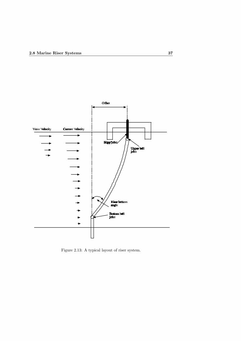
2.8 Marine Riser Systems 37
Figure 2.13: A typical layout of riser system.
38 Mathematical Modelling
Table 2.2: Strees joint specifications, Outer diameter (OD), inner diameter (ID).Type OD upper OD lower ID Length Yield StrengthType 1 184[mm] 273[mm] 133[mm] 10.67[m] 551 [MPa]Type 2 169[mm] 235[mm] 131[mm] 15.24[m] 517 [MPa]
2.8.1 Dynamic Model of Marine Risers
Depending on the assumptions and aims of analysis, different models for marinerisers have been derived, Morgan & Peret (n.d.), Burke (1974). The analysis modelof the marine risers is based on the general differential equation for a beam. Acommonly used model for dynamic riser motion is as in (2.28), where it is assumedthat P (x, t) = P =Constant. The third term is the radial force per unit lengthrequired to develop hoop tension in a cable configured as a circular arc. This termis the most effective term in the equation, since the conventional riser is essentiallya cable resisting lateral loads by tensile strength of the riser.
2.8.2 Boundary Conditions
At the sea floor, drilling and production risers are attached to the Blowout Pre-venter (BOP) through a special segment called stress joint, see Figure 2.15. Thissegment is designed to resist the large bending moments, but flexible to accom-modate the maximum riser displacements. Specifications for two stress joints arepresented in Table 2.2. Ball joints or flex joints are also used to connect the riserto the BOP, which is in turn connected to the well-head. The latter types ofconnection can accommodate larger misalignment due to vessel offset and riser de-flection up to 10 degrees. Hence, the bottom end of the riser has zero translationaldisplacement, velocity and acceleration, but depending on the connecting devicemay have a nonzero slope.
At the top end, the riser is connected to the floating vessel by a ball joint andtelescopic joint. A telescopic joint has an outer barrel which is connected to theriser, an inner barrel which is connected to the floating vessel, and a tensionerring which transmits loads from the tensioner system to the outer barrel of theriser. The basic function of the telescopic joint is to compensate for the relativetranslational movement between the vessel and the riser. The outer barrel providesstructural support for riser tensioner loads. In general, the motion of a vessel hassix degrees of freedom. Because of the ball joint and slip joint installed, onlysway, surge and heave modes have a significant effect on the riser system response.However, under controller design we will assume that a DP system is designed forthe vessel. Further, it will be assumed in analysis that the DP-system is perfectsuch that we can ignore the vessel-induced motion. Figure (2.14) shows a typicalmarine riser with associated equipments at boudaries.
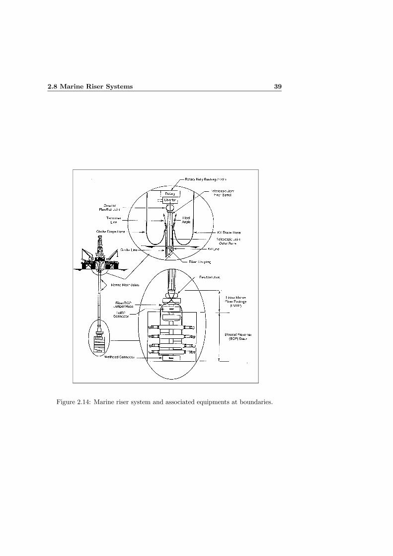
2.8 Marine Riser Systems 39
Figure 2.14: Marine riser system and associated equipments at boundaries.
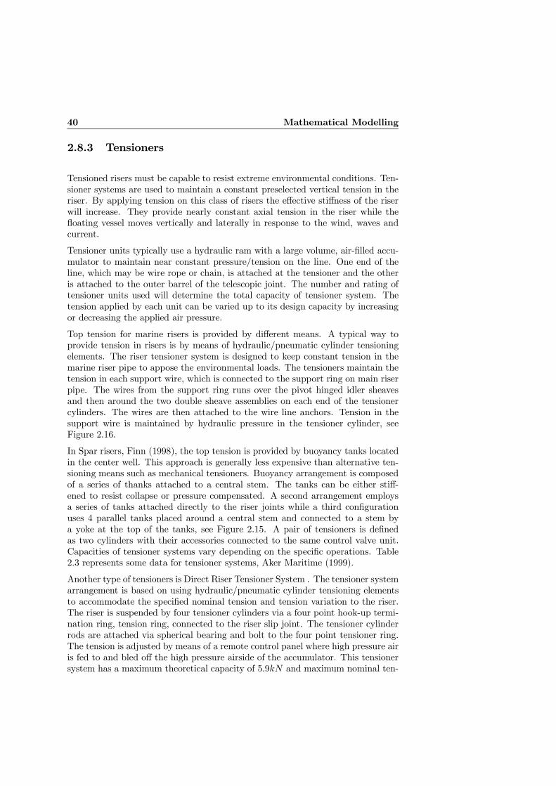
40 Mathematical Modelling
2.8.3 Tensioners
Tensioned risers must be capable to resist extreme environmental conditions. Ten-sioner systems are used to maintain a constant preselected vertical tension in theriser. By applying tension on this class of risers the effective stiffness of the riserwill increase. They provide nearly constant axial tension in the riser while thefloating vessel moves vertically and laterally in response to the wind, waves andcurrent.
Tensioner units typically use a hydraulic ram with a large volume, air-filled accu-mulator to maintain near constant pressure/tension on the line. One end of theline, which may be wire rope or chain, is attached at the tensioner and the otheris attached to the outer barrel of the telescopic joint. The number and rating oftensioner units used will determine the total capacity of tensioner system. Thetension applied by each unit can be varied up to its design capacity by increasingor decreasing the applied air pressure.
Top tension for marine risers is provided by different means. A typical way toprovide tension in risers is by means of hydraulic/pneumatic cylinder tensioningelements. The riser tensioner system is designed to keep constant tension in themarine riser pipe to appose the environmental loads. The tensioners maintain thetension in each support wire, which is connected to the support ring on main riserpipe. The wires from the support ring runs over the pivot hinged idler sheavesand then around the two double sheave assemblies on each end of the tensionercylinders. The wires are then attached to the wire line anchors. Tension in thesupport wire is maintained by hydraulic pressure in the tensioner cylinder, seeFigure 2.16.
In Spar risers, Finn (1998), the top tension is provided by buoyancy tanks locatedin the center well. This approach is generally less expensive than alternative ten-sioning means such as mechanical tensioners. Buoyancy arrangement is composedof a series of thanks attached to a central stem. The tanks can be either stiff-ened to resist collapse or pressure compensated. A second arrangement employsa series of tanks attached directly to the riser joints while a third configurationuses 4 parallel tanks placed around a central stem and connected to a stem bya yoke at the top of the tanks, see Figure 2.15. A pair of tensioners is definedas two cylinders with their accessories connected to the same control valve unit.Capacities of tensioner systems vary depending on the specific operations. Table2.3 represents some data for tensioner systems, Aker Maritime (1999).
Another type of tensioners is Direct Riser Tensioner System . The tensioner systemarrangement is based on using hydraulic/pneumatic cylinder tensioning elementsto accommodate the specified nominal tension and tension variation to the riser.The riser is suspended by four tensioner cylinders via a four point hook-up termi-nation ring, tension ring, connected to the riser slip joint. The tensioner cylinderrods are attached via spherical bearing and bolt to the four point tensioner ring.The tension is adjusted by means of a remote control panel where high pressure airis fed to and bled off the high pressure airside of the accumulator. This tensionersystem has a maximum theoretical capacity of 5.9kN and maximum nominal ten-
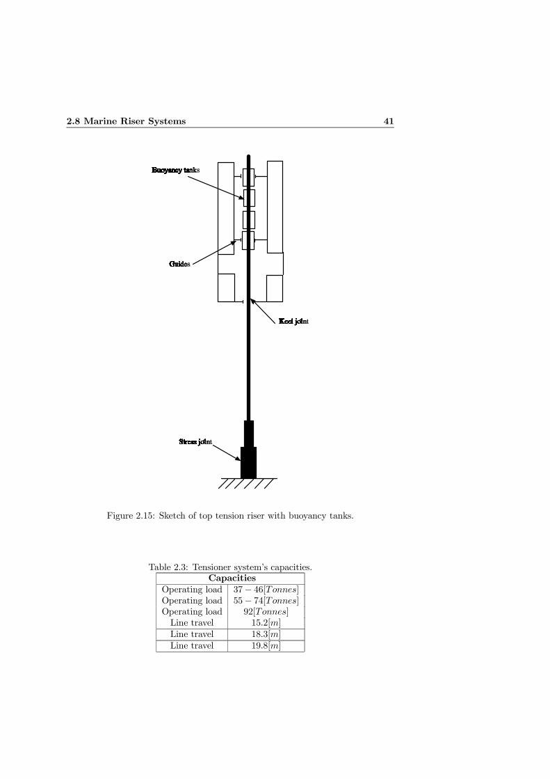
2.8 Marine Riser Systems 41
Figure 2.15: Sketch of top tension riser with buoyancy tanks.
Table 2.3: Tensioner system’s capacities.Capacities
Operating load 37− 46[Tonnes]Operating load 55− 74[Tonnes]Operating load 92[Tonnes]Line travel 15.2[m]Line travel 18.3[m]Line travel 19.8[m]
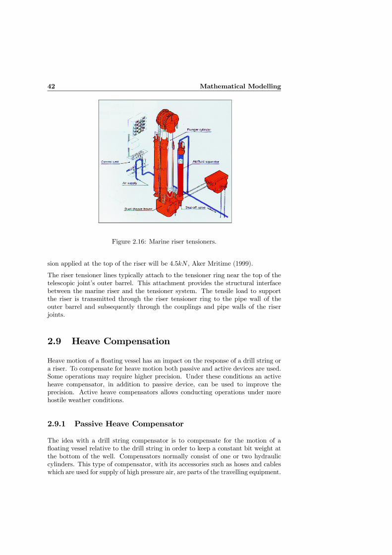
42 Mathematical Modelling
Figure 2.16: Marine riser tensioners.
sion applied at the top of the riser will be 4.5kN , Aker Mritime (1999).
The riser tensioner lines typically attach to the tensioner ring near the top of thetelescopic joint’s outer barrel. This attachment provides the structural interfacebetween the marine riser and the tensioner system. The tensile load to supportthe riser is transmitted through the riser tensioner ring to the pipe wall of theouter barrel and subsequently through the couplings and pipe walls of the riserjoints.
2.9 Heave Compensation
Heave motion of a floating vessel has an impact on the response of a drill string ora riser. To compensate for heave motion both passive and active devices are used.Some operations may require higher precision. Under these conditions an activeheave compensator, in addition to passive device, can be used to improve theprecision. Active heave compensators allows conducting operations under morehostile weather conditions.
2.9.1 Passive Heave Compensator
The idea with a drill string compensator is to compensate for the motion of afloating vessel relative to the drill string in order to keep a constant bit weight atthe bottom of the well. Compensators normally consist of one or two hydrauliccylinders. This type of compensator, with its accessories such as hoses and cableswhich are used for supply of high pressure air, are parts of the travelling equipment.
2.9 Heave Compensation 43
Figure 2.17: Top Mounted Drill String Compensator.
A Top Mounted Drill String Compensator is shown in Figure 2.17, where thedifferent components are:
1. Single unit steel structure
2. Two compensator units and air-oil medium separator
3. Dual Rocker-Arm system for fastline and deadline
4. Crown block
2.9.2 Active Heave Compensator
Active heave compensators are used in combination with passive drill string com-pensators to provide a stable position of the crown block referred to seabed. Thissystem is based on a hydraulic cylinder installed on top of the passive crown blockcompensator. The cylinder is suspended by specially designed spherical bearings.The cylinder is operated in such a way that it applies force to the crown blockto overcome frictions. The result is that the crown block position with respect toseabed is constant within 0.1−0.5 m with rig heave up to 4−5 m, Aker Maritime(1998). The cylinder is controlled by means of input from a heave motion sensor(3 axis accelerometer) and from a cylinder position sensor see Figure 2.18. Actingcylinders are attached directly between the crown block and the structure of thederrick. The active compensator is not a part of travelling equipment.
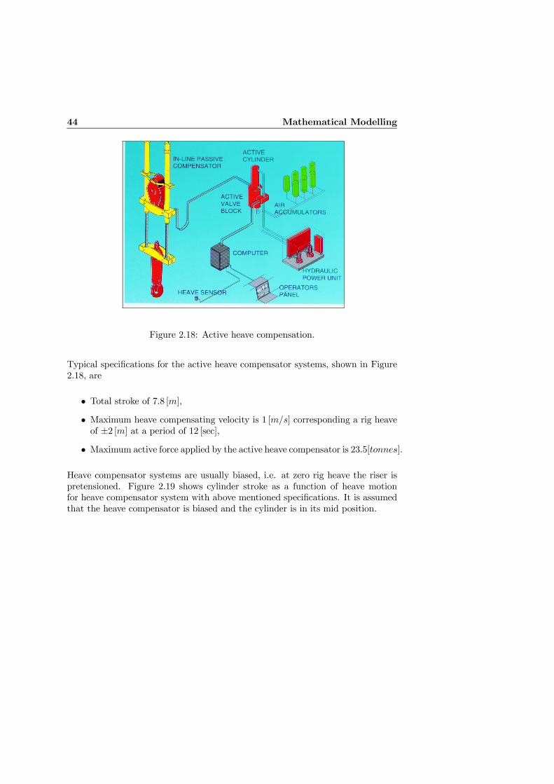
44 Mathematical Modelling
Figure 2.18: Active heave compensation.
Typical specifications for the active heave compensator systems, shown in Figure2.18, are
• Total stroke of 7.8 [m],• Maximum heave compensating velocity is 1 [m/s] corresponding a rig heaveof ±2 [m] at a period of 12 [sec],
• Maximum active force applied by the active heave compensator is 23.5[tonnes].
Heave compensator systems are usually biased, i.e. at zero rig heave the riser ispretensioned. Figure 2.19 shows cylinder stroke as a function of heave motionfor heave compensator system with above mentioned specifications. It is assumedthat the heave compensator is biased and the cylinder is in its mid position.
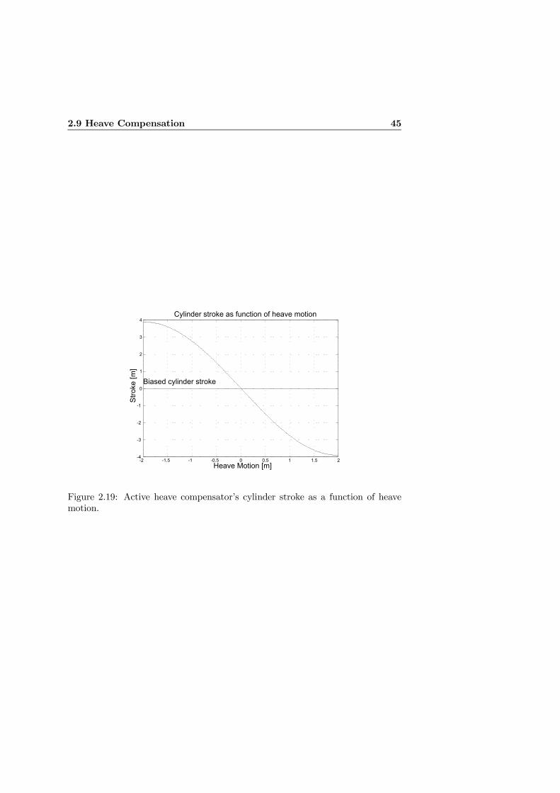
2.9 Heave Compensation 45
-2 -1.5 -1 -0.5 0 0.5 1 1.5 2-4
-3
-2
-1
0
1
2
3
4
Heave Motion [m]
Stro
ke [m
]
Cylinder stroke as function of heave motion
Biased cylinder stroke
Figure 2.19: Active heave compensator’s cylinder stroke as a function of heavemotion.

46 Mathematical Modelling
Chapter 3
Passivity Analysis ofNonlinear Beams
It is well known that certain combination of passive and strictly passive systemsresults in passivity or srict passivity of the closed-loop system. The idea thata simple structure controller, like a proportional controller from velocity, can beused in combination with a passive plant to ensure the stability of the closed-loopsystem is attractive from the implementational point of view. Passivity propertiesof distributed parameter systems have been investigated very little in their originalform, i.e. PDE’s. There are few papers which exploits this property of the originalmodels to design control laws. In Matsuno & Murata (1999) the passivity proper-ties of one-link and two-link flexible arms, in theirs original distributed-parametermodels, are investigated. Aamo & Fossen (1999) proves the passivity of a mooringsystem, described in PDE form. Then, it is concluded that passive control lawsin combination with the mooring system ensure stability of the total system. Inthis chapter the passivity properties of beams in vibration are investigated. Firstthe coupled dynamic system, (3.1)-(3.2) with its boundary conditions, (3.3a)-(3.4)is considered. The dynamics of transverse bending of a beam, (3.6), will be in-vestigated. Finally we introduce a control mechanism which is attached to thetop boundary of the beam and the passivity properties of the combined system isinvestigated. The results from this chapter have been presented in Fard & Sagatun(2000c).
48 Passivity Analysis of Nonlinear Beams
3.1 Coupled Dynamic System
Consider the equations of motion for a nonlinear beam
ρA∂2η(x, t)
∂t2+
∂2
∂x2
µEI
∂2η(x, t)
∂x2
¶− ∂
∂x
µEA
∂µ(x, t)
∂x
∂η(x, t)
∂x
¶−P0 ∂
2η(x, t)
∂x2− 12
∂
∂x
ÃEA
µ∂η(x, t)
∂x
¶3!− f(x, t) = 0 (3.1)
ρA∂2µ(x, t)
∂t2− ∂
∂x
µEA
∂µ(x, t)
∂x
¶− 12
∂
∂x
ÃEA
µ∂η(x, t)
∂x
¶2!= 0 (3.2)
where EI denotes the flexural rigidity per unit length of the beam, ρA is mass perunit length of the beam, E is the Youg’s modudlus of elasticity. µ(x, t) and η(x, t)denote longitudinal displacement and transverse deflection at time t with respectto the spatial variable x, respectively. Boundary conditions are
η(x, t) = 0 at x = 0 (3.3a)
µ(x, t) = 0 at x = 0 (3.3b)
EI∂2η(x, t)
∂x2= 0 at x = 0, L. (3.3c)
It is assumed that the system’s input, u1(t), is at the top boundary of the beam,i.e.,
1
2EA
µ∂η(x, t)
∂x
¶2+EA
∂µ(x, t)
∂x= u1(t), at x = L (3.4)
Proposition 1
The system (3.1)-(3.2) with the boundary conditions (3.3a)-(3.4) is lossless passive,see Appendix A, when the output y1(t) is given as
y1(t) = µt(L, t).
Proof : Consider the storage function
V (t) =ρA
2
Z L
0
η2t (x, t)dx+ρA
2
Z L
0
µ2t (x, t)dx+P02
Z L
0
η2x(x, t)dx
+EI
2
Z L
0
η2xx(x, t)dx+EA
2
Z L
0
µµx(x, t) +
1
2η2x(x, t)
¶2dx
The derivative of V (t) with respect to time, using the results of Lemmas 4.1 and5.1, yields
V (t) = −EI ηxxxηt|L0 +EI ηxxηtx|L0EA
2η3xηt
¯L0+EA µxµt|L0 + P0 ηxηt|L0
+EA ηxµxηt|L0 +EA1
2η2xµt
¯L0
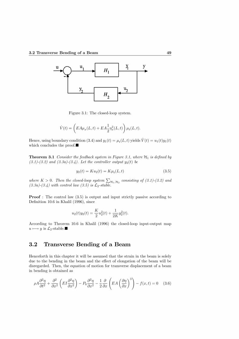
3.2 Transverse Bending of a Beam 49
Figure 3.1: The closed-loop system.
V (t) =
µEAµx(L, t) +EA
1
2η2x(L, t)
¶µt(L, t).
Hence, using boundary condition (3.4) and y1(t) = µt(L, t) yields V (t) = u1(t)y1(t)which concludes the proof.¥
Theorem 3.1 Consider the feedback system in Figure 3.1, where H1 is defined by(3.1)-(3.2) and (3.3a)-(3.4). Let the controller output y2(t) be
y2(t) = Ku2(t) = Kµt(L, t) (3.5)
where K > 0. Then the closed-loop systemPH1,H2
consisting of (3.1)-(3.2) and(3.3a)-(3.4) with control law (3.5) is L2-stable.
Proof : The control law (3.5) is output and input strictly passive according toDefinition 10.6 in Khalil (1996), since
u2(t)y2(t) =K
2u22(t) +
1
2Ky22(t).
According to Theorem 10.6 in Khalil (1996) the closed-loop input-output mapu 7−→ y is L2-stable.¥
3.2 Transverse Bending of a Beam
Henceforth in this chapter it will be assumed that the strain in the beam is solelydue to the bending in the beam and the effect of elongation of the beam will bedisregarded. Then, the equation of motion for transverse displacement of a beamin bending is obtained as
ρA∂2η
∂t2+
∂2
∂x2
µEI
∂2η
∂x2
¶− P0 ∂
2η
∂x2− 12
∂
∂x
ÃEA
µ∂η
∂x
¶3!− f(x, t) = 0 (3.6)
50 Passivity Analysis of Nonlinear Beams
∀ (x, t) ∈ (0, L)× [0,∞), with the following boundary conditions
η(x, t) = 0 at x = 0 (3.7a)
EI∂2η(x, t)
∂x2= 0 at x = 0, L (3.7b)
− ∂
∂x
µEI
∂2η
∂x2
¶+ P0
∂η
∂x+1
2EA
µ∂η
∂x
¶3= u1(t) at x = L. (3.7c)
Proposition 2
The system (3.6) with boundary conditions (3.7a)-(3.7c) is lossless passive,when the output y1(t) is given as
y1(t) = ηt(L, t).
Proof : Consider the storage function
V (t) =ρA
2
Z L
0
η2t (x, t)dx+P02
Z L
0
η2x(x, t)dx
+EA
8
Z L
0
η4x(x, t)dx+EI
2
Z L
0
η2xx(x, t)dx. (3.8)
The derivative of V (t) with respect to time, using the results of the Lemma 4.1,yields
V (t) =
µ−EIηxxx(L, t) +
EA
2η3x(L, t) + P0ηx(L, t)
¶ηt(L, t).
Hence, using the boundary condition (3.7c) and y1(t) = ηt(L, t) yields V (t) =u1(t)y1(t) which concludes the proof.¥
Theorem 3.2 Consider the feedback system in Figure 3.1, where H1 is defined by(3.6) and (3.7a)-(3.7c). Let the controller output y2(t) be
y2(t) = Ku2(t) = Kηt(L, t) (3.9)
where K > 0. Then the closed-loop systemPH1,H2
consisting of (3.6) and (3.7a)-(3.7c) with control law (3.9) is L2-stable.
Proof : The control law (3.9) is output and input strictly passive according toDefinition 10.6 in Khalil (1996), since
u2(t)y2(t) =K
2u22(t) +
1
2Ky22(t).
According to Theorem 10.6 in Khalil (1996) the closed-loop input-output mapu 7−→ y is L2-stable.¥
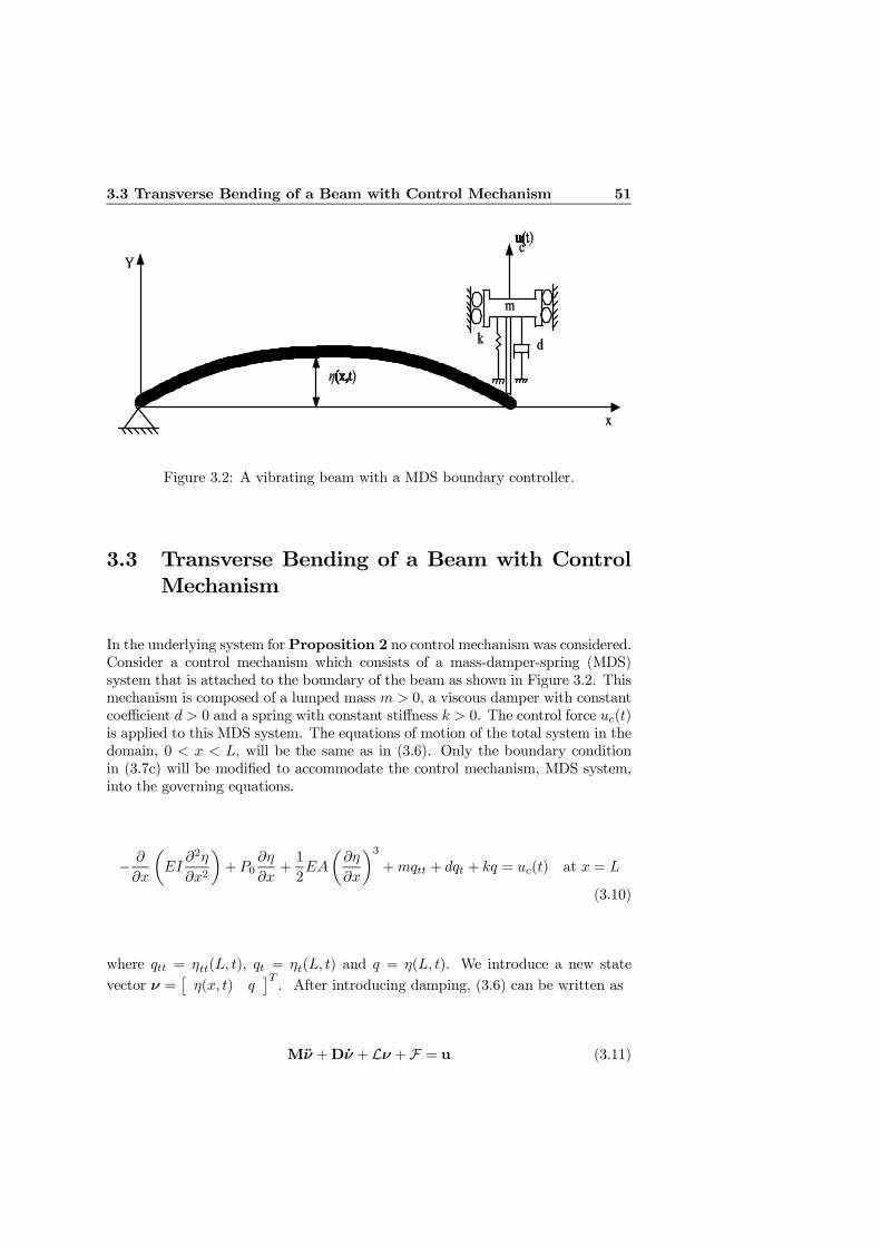
3.3 Transverse Bending of a Beam with Control Mechanism 51
Figure 3.2: A vibrating beam with a MDS boundary controller.
3.3 Transverse Bending of a Beam with ControlMechanism
In the underlying system forProposition 2 no control mechanism was considered.Consider a control mechanism which consists of a mass-damper-spring (MDS)system that is attached to the boundary of the beam as shown in Figure 3.2. Thismechanism is composed of a lumped mass m > 0, a viscous damper with constantcoefficient d > 0 and a spring with constant stiffness k > 0. The control force uc(t)is applied to this MDS system. The equations of motion of the total system in thedomain, 0 < x < L, will be the same as in (3.6). Only the boundary conditionin (3.7c) will be modified to accommodate the control mechanism, MDS system,into the governing equations.
− ∂
∂x
µEI
∂2η
∂x2
¶+ P0
∂η
∂x+1
2EA
µ∂η
∂x
¶3+mqtt + dqt + kq = uc(t) at x = L
(3.10)
where qtt = ηtt(L, t), qt = ηt(L, t) and q = η(L, t). We introduce a new statevector ν =
£η(x, t) q
¤T. After introducing damping, (3.6) can be written as
Mν +Dν + Lν +F = u (3.11)
52 Passivity Analysis of Nonlinear Beams
where
M =
·ρA 00 m
¸D =
·D 00 d
¸L =
"∂2
∂x2EI∂2
∂x2 − P0 ∂2
∂x2 0
0 − ∂∂xEI
∂2
∂x2 + P0∂∂x + k
#
F = −12 ∂
∂x
µEA
³∂η∂x
´3¶12EAη
3x
u =
·0
uc(t)
¸.
Proposition 3
The system (3.11) is output strictly passive, when
y(t) = qt(t) = ηt(L, t).
Proof: Consider the storage function
V (t) =ρA
2
Z L
0
η2t (x, t)dx+P02
Z L
0
η2x(x, t)dx
+EA
8
Z L
0
η4x(x, t)dx+EI
2
Z L
0
η2xx(x, t)dx
+1
2mq2t (t) +
1
2kmq
2(t). (3.12)
The derivative of V (t) with respect to time, using the results of the Lemma 4.1,yields
V (t) =
µ−EIηxxx(L, t) +
EA
2η3x(L, t) + P0ηx(L, t)
¶ηt(L, t)
+mqttqt + kqqt.
=
µ−EIηxxx(L, t) +
EA
2η3x(L, t) + P0ηx(L, t) +mqtt + kq
¶qt
Using the boundary condition (3.10) and y(t) = qt(t) we obtain
uc(t)y(t) = V (t) + dy2(t)
and hence the proof is completed.¥
Theorem 3.3 Consider the closed-loop systemPM,H in Figure 3.3, where
M : uc(t) 7−→ ηt(L, t)
H : ηt(L, t) 7−→ u(t).
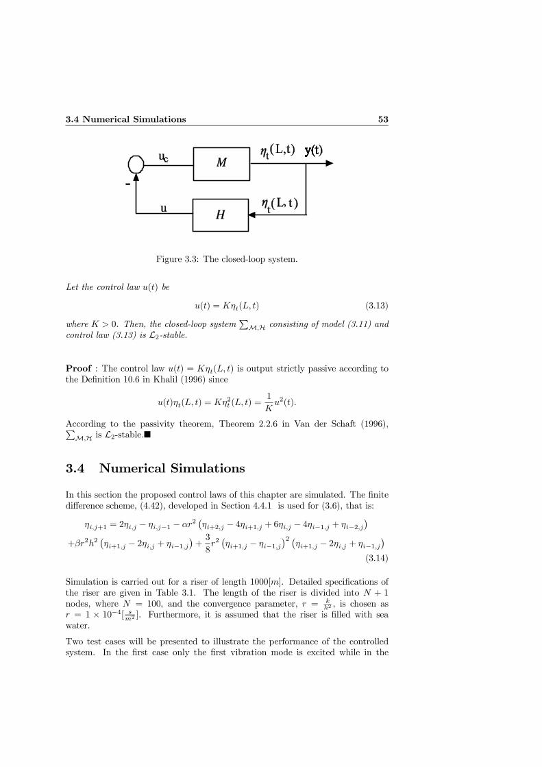
3.4 Numerical Simulations 53
Figure 3.3: The closed-loop system.
Let the control law u(t) be
u(t) = Kηt(L, t) (3.13)
where K > 0. Then, the closed-loop systemPM,H consisting of model (3.11) and
control law (3.13) is L2-stable.
Proof : The control law u(t) = Kηt(L, t) is output strictly passive according tothe Definition 10.6 in Khalil (1996) since
u(t)ηt(L, t) = Kη2t (L, t) =1
Ku2(t).
According to the passivity theorem, Theorem 2.2.6 in Van der Schaft (1996),PM,H is L2-stable.¥
3.4 Numerical Simulations
In this section the proposed control laws of this chapter are simulated. The finitedifference scheme, (4.42), developed in Section 4.4.1 is used for (3.6), that is:
ηi,j+1 = 2ηi,j − ηi,j−1 − αr2¡ηi+2,j − 4ηi+1,j + 6ηi,j − 4ηi−1,j + ηi−2,j
¢+βr2h2
¡ηi+1,j − 2ηi,j + ηi−1,j
¢+3
8r2¡ηi+1,j − ηi−1,j
¢2 ¡ηi+1,j − 2ηi,j + ηi−1,j
¢(3.14)
Simulation is carried out for a riser of length 1000[m]. Detailed specifications ofthe riser are given in Table 3.1. The length of the riser is divided into N + 1nodes, where N = 100, and the convergence parameter, r = k
h2 , is chosen asr = 1 × 10⁻⁴[ sm2 ]. Furthermore, it is assumed that the riser is filled with seawater.
Two test cases will be presented to illustrate the performance of the controlledsystem. In the first case only the first vibration mode is excited while in the
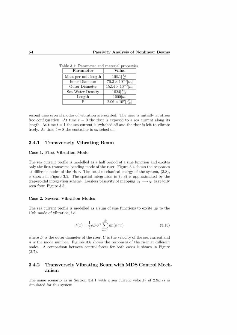
54 Passivity Analysis of Nonlinear Beams
Table 3.1: Parameter and material properties.Parameter Value
Mass per unit length 108.1[kgm ]Inner Diameter 76.2× 10⁻³[m]Outer Diameter 152.4× 10⁻³[m]Sea Water Density 1024[ kgm3 ]
Length 1000[m]
E 2.06× 10⁹[ Nm2 ]
second case several modes of vibration are excited. The riser is initially at stressfree configuration. At time t = 0 the riser is exposed to a sea current along itslength. At time t = 1 the sea current is switched off and the riser is left to vibratefreely. At time t = 8 the controller is switched on.
3.4.1 Transversely Vibrating Beam
Case 1. First Vibration Mode
The sea current profile is modelled as a half period of a sine function and excitesonly the first transverse bending mode of the riser. Figure 3.4 shows the responsesat different nodes of the riser. The total mechanical energy of the system, (3.8),is shown in Figure 3.5. The spatial integration in (3.8) is approximated by thetrapezoidal integration scheme. Lossless passivity of mapping u1 7−→ y1 is readilyseen from Figure 3.5.
Case 2. Several Vibration Modes
The sea current profile is modelled as a sum of sine functions to excite up to the10th mode of vibration, i.e.
f(x) =1
2ρDU2
10Xn=1
sin(nπx) (3.15)
where D is the outer diameter of the riser, U is the velocity of the sea current andn is the mode number. Figures 3.6 shows the responses of the riser at differentnodes. A comparison between control forces for both cases is shown in Figure(3.7).
3.4.2 Transversely Vibrating BeamwithMDSControl Mech-anism
The same scenario as in Section 3.4.1 with a sea current velocity of 2.9m/s issimulated for this system.
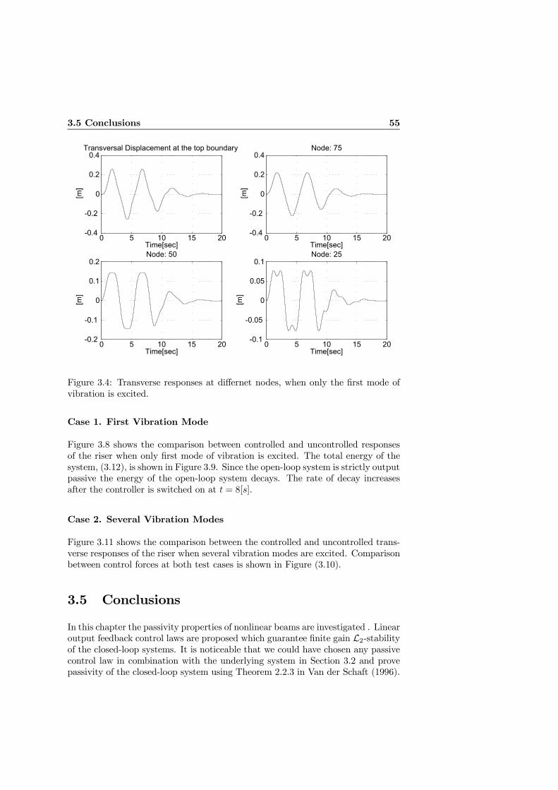
3.5 Conclusions 55
0 5 10 15 20-0.4
-0.2
0
0.2
0.4Transversal Displacement at the top boundary
[m]
Time[sec]0 5 10 15 20-0.4
-0.2
0
0.2
0.4Node: 75
[m]
Time[sec]
0 5 10 15 20-0.2
-0.1
0
0.1
0.2Node: 50
[m]
Time[sec]0 5 10 15 20-0.1
-0.05
0
0.05
0.1Node: 25
[m]
Time[sec]
Figure 3.4: Transverse responses at differnet nodes, when only the first mode ofvibration is excited.
Case 1. First Vibration Mode
Figure 3.8 shows the comparison between controlled and uncontrolled responsesof the riser when only first mode of vibration is excited. The total energy of thesystem, (3.12), is shown in Figure 3.9. Since the open-loop system is strictly outputpassive the energy of the open-loop system decays. The rate of decay increasesafter the controller is switched on at t = 8[s].
Case 2. Several Vibration Modes
Figure 3.11 shows the comparison between the controlled and uncontrolled trans-verse responses of the riser when several vibration modes are excited. Comparisonbetween control forces at both test cases is shown in Figure (3.10).
3.5 Conclusions
In this chapter the passivity properties of nonlinear beams are investigated . Linearoutput feedback control laws are proposed which guarantee finite gain L2-stabilityof the closed-loop systems. It is noticeable that we could have chosen any passivecontrol law in combination with the underlying system in Section 3.2 and provepassivity of the closed-loop system using Theorem 2.2.3 in Van der Schaft (1996).
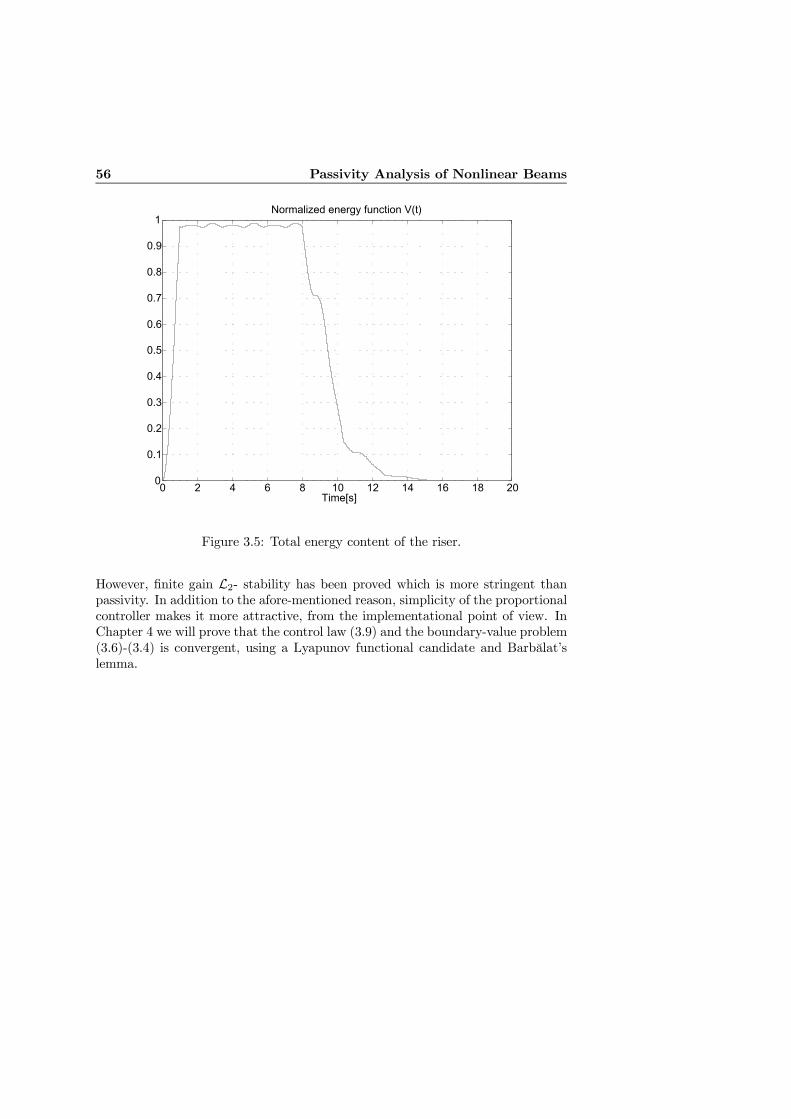
56 Passivity Analysis of Nonlinear Beams
0 2 4 6 8 10 12 14 16 18 200
0.1
0.2
0.3
0.4
0.5
0.6
0.7
0.8
0.9
1
Time[s]
Normalized energy function V(t)
Figure 3.5: Total energy content of the riser.
However, finite gain L2- stability has been proved which is more stringent thanpassivity. In addition to the afore-mentioned reason, simplicity of the proportionalcontroller makes it more attractive, from the implementational point of view. InChapter 4 we will prove that the control law (3.9) and the boundary-value problem(3.6)-(3.4) is convergent, using a Lyapunov functional candidate and Barbalat’slemma.
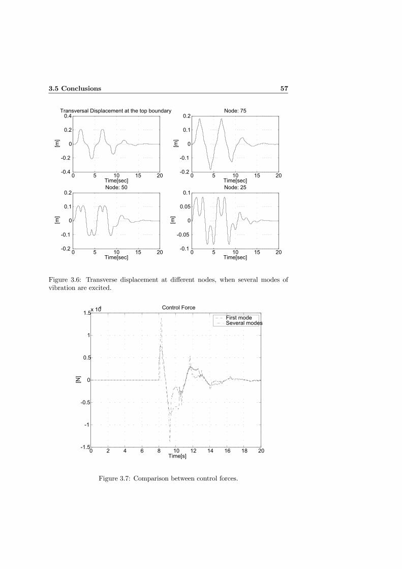
3.5 Conclusions 57
0 5 10 15 20-0.4
-0.2
0
0.2
0.4Transversal Displacement at the top boundary
[m]
Time[sec]0 5 10 15 20-0.2
-0.1
0
0.1
0.2Node: 75
[m]
Time[sec]
0 5 10 15 20-0.2
-0.1
0
0.1
0.2Node: 50
[m]
Time[sec]0 5 10 15 20-0.1
-0.05
0
0.05
0.1Node: 25
[m]
Time[sec]
Figure 3.6: Transverse displacement at different nodes, when several modes ofvibration are excited.
0 2 4 6 8 10 12 14 16 18 20-1.5
-1
-0.5
0
0.5
1
1.5x 10⁴ Control Force
Time[s]
[N]
First mode Several modes
Figure 3.7: Comparison between control forces.
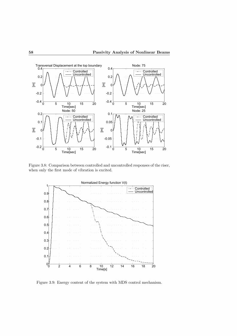
58 Passivity Analysis of Nonlinear Beams
0 5 10 15 20-0.4
-0.2
0
0.2
0.4Transversal Displacement at the top boundary
[m]
Time[sec]
Controlled Uncontrolled
0 5 10 15 20-0.4
-0.2
0
0.2
0.4Node: 75
[m]
Time[sec]
Controlled Uncontrolled
0 5 10 15 20-0.2
-0.1
0
0.1
0.2Node: 50
[m]
Time[sec]
Controlled Uncontrolled
0 5 10 15 20-0.1
-0.05
0
0.05
0.1Node: 25
[m]
Time[sec]
Controlled Uncontrolled
Figure 3.8: Comparison between controlled and uncontrolled responses of the riser,when only the first mode of vibration is excited.
0 2 4 6 8 10 12 14 16 18 200
0.1
0.2
0.3
0.4
0.5
0.6
0.7
0.8
0.9
1Normalized Energy function V(t)
Time[s]
Controlled Uncontrolled
Figure 3.9: Energy content of the system with MDS control mechanism.
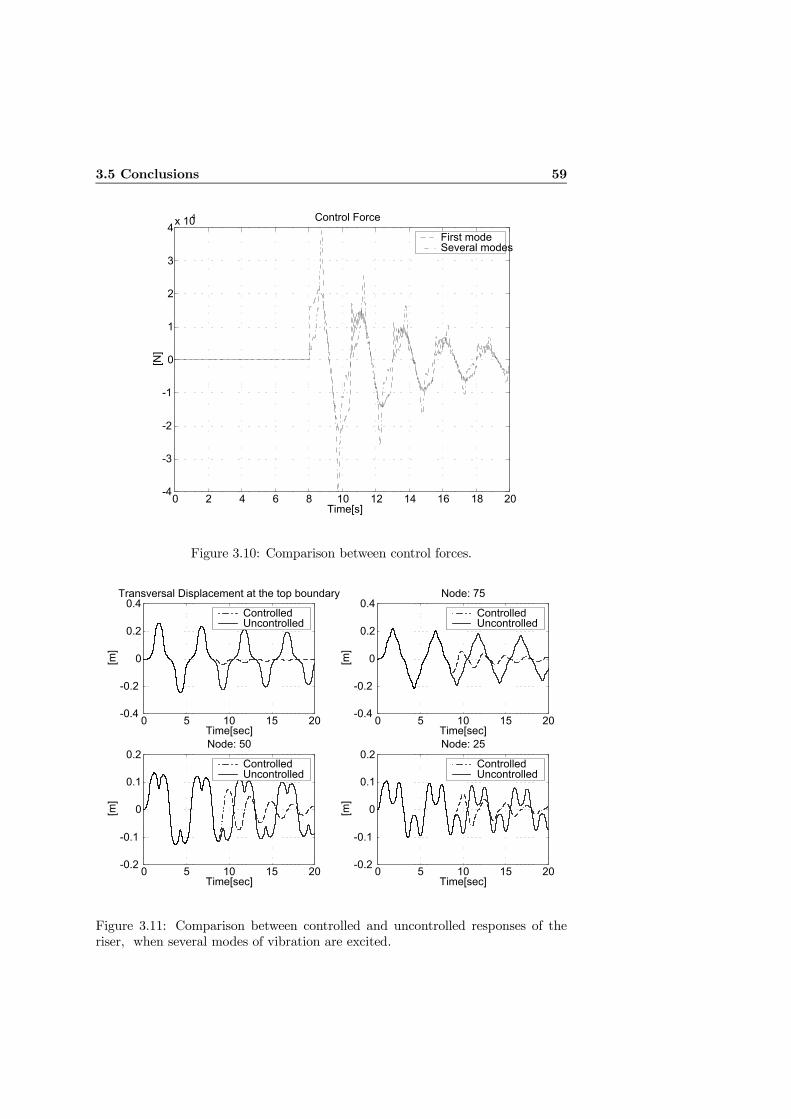
3.5 Conclusions 59
0 2 4 6 8 10 12 14 16 18 20-4
-3
-2
-1
0
1
2
3
4x 10⁴
Time[s]
[N]
Control Force
First mode Several modes
Figure 3.10: Comparison between control forces.
0 5 10 15 20-0.4
-0.2
0
0.2
0.4Transversal Displacement at the top boundary
[m]
Time[sec]
Controlled Uncontrolled
0 5 10 15 20-0.4
-0.2
0
0.2
0.4Node: 75
[m]
Time[sec]
Controlled Uncontrolled
0 5 10 15 20-0.2
-0.1
0
0.1
0.2Node: 50
[m]
Time[sec]
Controlled Uncontrolled
0 5 10 15 20-0.2
-0.1
0
0.1
0.2Node: 25
[m]
Time[sec]
Controlled Uncontrolled
Figure 3.11: Comparison between controlled and uncontrolled responses of theriser, when several modes of vibration are excited.

60 Passivity Analysis of Nonlinear Beams
Chapter 4
Boundary Control of aTransversely VibratingBeam
The control problem of beams in vibration are considered in this and the sub-sequent chapter. In this chapter the transverse dynamics of a beam in bendingvibration is considered, while the coupling between longitudinal and transversaldynamics is neglected. Some of the results of the work in this chapter have beenpresented in Fard & Sagatun (1999) and Fard & Sagatun (2000a).
4.1 Equations of Motion
The dynamic equations of motion of a modified, nonlinear Euler-Bernoulli beamwas derived in Chapter 2, and we restate the equations here for convenience,
ρAηtt(x, t) +EIηxxxx(x, t)− P0ηxx(x, t)−3
2EAηxx(x, t)η
2x(x, t)− f(x, t) = 0
(4.1)
∀ (x, t) ∈ (0, L) × [0,∞). Both flexural rigidity, EI, and mass per unit length,ρA, are assumed to be constant. The discussion will be limited to freely vibratingbeams; hence, f(x, t) will be set to zero.
In (4.1) the notations ηtt(x, t) =∂2η(x,t)∂t2 , ηxx(x, t) =
∂2η(x,t)∂x2 and ηx(x, t) =
∂η(x,t)∂x
are used. Note that the (4.1) is identical with (2.28), if we assume that the axialstrain-displacement relationship in (2.28) is given by
P (x, t) = P0 +1
2EAη2x(x, t).
Only the elongation of the beam due to bending is considered here. The variationof the length due to axial force is assumed small in comparison with the total
62 Boundary Control of a Transversely Vibrating Beam
length of the beam and negligible. The boundary conditions are
EIηxx(0, t) = EIηxx(L, t) = 0 (4.2a)
η(0, t) = 0 (4.2b)
u(t) = −EIηxxx(L, t) + P0ηx(L, t) +1
2EAη3x(L, t) (4.2c)
where boundary condition (4.2a) represents the bending moments at the bound-aries. Equation (4.2c) denotes the shear force at x = L of the beam. u(t) repre-sents the boundary control force applied at x = L. The boundary condition (4.2c)represents the balance of the shear force and the control force u(t). The initialconditions are
η(x, 0) = g1(x) (4.3)
ηt(x, 0) = g2(x) (4.4)
∀ (x, t) ∈ (0, L)× [0,∞). Equations (4.3) and (4.4) denote the initial position andvelocity functions, respectively.
The main objective is to construct a control law, u(t), which stabilizes the nonlinearequation of the beam (4.1), (4.2a)-(4.2c) and guarantees that η(x, t)→ 0 as t→∞for all x ∈ [0, L].
4.1.1 Assumptions
Assumption 4.1 It will be assumed that:
1. P0 is a tensile force, i.e. P0 > 0 for all t ≥ 0. This assumption simplymeans that an axially tensioned beam is considered. P0 < 0 corresponds toa compressed beam.
2. There exists a solution for the dynamics given by (4.1) and (4.2a)-(4.2c).It is also assumed that the deflection η(x, t) and its time derivative ηt(x, t)belong to a space of functions which have the following properties:
i) If the potential energy of the system is proven to be bounded ∀t ∈ [0,∞),then ∂nη(x,t)
∂xn is bounded for n = 3, 4, ∀(x, t) ∈ [0, L]× [0,∞), andii) If the kinetic energy of the system is proven to be bounded ∀t ∈ [0,∞),
then ∂nηt(x,t)∂xn is bounded for n = 1, 2, 3, ∀(x, t) ∈ [0, L]× [0,∞).
4.2 Design of Boundary Control
The control objective is to design a control law which guarantees stability of thedistributed-parameter system consisting (4.1) and (4.2a)-(4.2c), using the bound-ary control (4.2c).
4.2 Design of Boundary Control 63
In subsequent stability analysis some identities are needed which will be proved inthe following lemma.
Lemma 4.1 Let η(x, t) be the solution of (4.1) which satisfy the boundary condi-tions (4.2a)-(4.2c). Then
−EIZ L
0
[ηxxxxηt − ηxxηxxt] dx = −EIhηxxxηt|L0 − ηxxηtx|L0
i(4.5)
EA
2
Z L
0
£η3xηxt + 3η
2xηxxηt
¤dx =
EA
2η3xηt
¯L0
(4.6)
P0
Z L
0
[ηxxηt + ηxηxt] dx = P0 ηxηt|L0 (4.7)
−γEIZ L
0
xηxxxxηxdx = −γ3EI
2
Z L
0
η2xxdx
−γEI·L
µηxxx(L, t)ηx(L, t)−
1
2η2xx(L, t)
¶− ηxxηx|L0
¸(4.8)
γP0
Z L
0
xηxxηxdx = γP0
"L
2η2x(L, t)−
1
2
Z L
0
η2xdx
#(4.9)
γ3
2EA
Z L
0
xη3xηxxdx = γ3
2EA
ÃL
4η4x(L, t)−
1
4
Z L
0
η4xdx
!(4.10)
γρA
Z L
0
xηtηtxdx = γρA
"L
2η2t (L, t)−
1
2
Z L
0
η2tdx
#(4.11)
∀ t ≥ 0.
Proof : See Appendix B¥.
4.2.1 Convergent Control Law
The following Lyapunov functional is introduced:
V (t) =ρA
2
Z L
0
η2t (x, t)dx+P02
Z L
0
η2x(x, t)dx
+EA
8
Z L
0
η4x(x, t)dx+EI
2
Z L
0
η2xx(x, t)dx (4.12)
∀ t ≥ 0, where η(·, ·) satisfies the boundary-value problem (4.1) and (4.2a)-(4.2c).Note that V (t) represents the mechanical potential and kinetic energies of thesystem. The first term represents the kinetic energy, the second and third termsrepresent the strain energy while the fourth term represents the potential energydue to bending.
64 Boundary Control of a Transversely Vibrating Beam
Theorem 4.1 Let the boundary control law u(t) in (4.2c), be
u(t) = −Kηt(L, t) (4.13)
where K > 0. Then, the functional V (t) along the solution of the system (4.1),with corresponding boundary conditions, (4.2a)-(4.2c), satisfies
V (t) = −Kηt(L, t)2. (4.14)
Hence, the states of the system, ηt(x, t), ηx(x, t), ηxx(x, t) and η(x, t) are boundedand converge to zero.
Proof The derivative of (4.12) with respect to time is given by (for the sake ofsimplicity the argument (x, t) is omitted)
V (t) = ρA
Z L
0
ηttηtdx+ P0
Z L
0
ηxηxtdx+EA
2
Z L
0
η3xηxtdx+EI
Z L
0
ηxxηxxtdx.
Substitution of ρAηtt from (4.1) into the expression for time derivation of Lya-punov functional yields
V (t) = −EIZ L
0
ηxxxxηtdx+ P0
Z L
0
ηxxηtdx+3
2EA
Z L
0
η2xηxxηtdx
+P0
Z L
0
ηxηxtdx+EA
2
Z L
0
η3xηxtdx+EI
Z L
0
ηxxηxxtdx. (4.15)
From boundary condition (4.2b) one can conclude that ηt(0, t) = 0 for all t ≥ 0.Hence by applying boundary condition (4.2a) and Lemma 4.1, we obtain
V (t) = −EIηxxx(L, t)ηt(L, t) +EA
2η3x(L, t)ηt(L, t) + P0ηx(L, t)ηt(L, t).
Now substitution for EIηxxx(L, t) from boundary condition (4.2c) and using con-trol law (4.13) yields (4.14). By this we can conclude that the states of the systemare bounded and remain bounded for all t ≥ 0. As a consequence both the kineticand the potential energies of the system, given by (4.12), are bounded. Due toboundedness of potential energy, we use property i of Assumption 4.1 to concludethat ∂nη(x,t)
∂xn is bounded for n = 3, 4, ∀(x, t) ∈ [0, L] × [0,∞). Furthermore, byusing property ii of Assumption 4.1 we conclude that ∂nηt(x,t)
∂xn is bounded forn = 1, 2, 3, ∀(x, t) ∈ [0, L]× [0,∞).In order to prove convergence of states, we need to establish that V (t) is uniformlycontinuous. To prove this it is sufficient to prove that V (t) is bounded ∀t ≥ t0.The time derivative of (4.14) is given by
V (t) = −2Kηt(L, t)ηtt(L, t).
Time differentiation of the boundary condition (4.2c) after substitution of controllaw (4.13) yields
−Kηtt(L, t) = −EIηxxxt(L, t) + P0ηxt(L, t) +3
2EAη2x(L, t)ηxt(L, t) . (4.16)
4.2 Design of Boundary Control 65
We have already established that ηt(L, t) is bounded ∀t ∈ [0,∞). Equation (4.1)and boundedness of ∂nη(x,t)
∂xn can be utilized to show that ηtt(x, t) is bounded
∀(x, t) ∈ (0, L)× [0,∞). Using (4.16), and boundedness of ∂nηt(x,t)∂xn for n = 1, 2, 3
we conclude that ηtt(L, t) is bounded ∀t ∈ [0,∞). Hence, according to Barbalat’slemma Barbâlat (1959), V (t) → 0 as t → ∞. Hence, the states of the systemconverge to zero as t → ∞. Now since η(0, t) = 0, ∀t ∈ [0,∞) and all statesconverges to zero as t → ∞. It is concluded that η(x, t) converges to zero ast→∞. Hence, the theorem is proven.¥
4.2.2 Exponentially Stabilizing Control Law
Consider the metric
ρ(q,0) =
"ρA
2
Z L
0
η2t (x, t)dx+P02
Z L
0
η2x(x, t)dx
+EA
8
Z L
0
η4x(x, t)dx+EI
2
Z L
0
η2xx(x, t)dx
# 12
(4.17)
where qT = [ηt ηx ηxx]. The metric ρ(q,0) establishes a measure of the closenessof the state q to the equilibrium null state in terms of the velocity, slope andcurvature of the beam. Further, if ρ(q,0) is small, then each of its terms mustthen also be small, as the integrand of ρ(q,0) is the sum of these non-negativeterms.
The Lyapunov functional V (t) is introduced:
V (t) = ρ2(q,0) + γρA
Z L
0
xηt(x, t)ηx(x, t)dx ∀t ≥ 0 (4.18)
where γ is a small positive constant real number.
Theorem 4.2 Let the boundary control law u(t) in (4.2c) be
u(t) = −K1ηx(L, t)−K2ηt(L, t) (4.19)
where
K1 ≥ −12γ2
L2
(γL− 1)2 ρA (4.20a)
K2 ≥ 1
2
1− 2γL(γL− 1)2 γLρA (4.20b)
and γL < 12 . Then, the functional V (t) along the solution of the system (4.1),
(4.2a)-(4.2c), satisfies
V (t) ≤ V (0) expµ− γ
1 + γγ1t
¶(4.21)
66 Boundary Control of a Transversely Vibrating Beam
where γ1 = Lmax(1,ρAP0). Furthermore,
ρ(q,0) ≤s1 + γγ11− γγ1
ρ(q(0),0) exp(− γ
2 (1 + γγ1)t). (4.22)
Hence, the equilibrium state q = 0 is exponentially stable.
In order to prove this theorem it is necessary to establish the following lemma.
Lemma 4.2 Let γ in (4.18) satisfy
γ ¿ 1
γ1. (4.23)
Then, the functional V (t) satisfies
(1− γγ1)ρ2(q,0) ≤ V (t) ≤ (1 + γγ1) ρ
2(q,0), ∀t ≥ 0. (4.24)
Furthermore V (t) is positive definite with respect to the metric ρ(q,0) and admitsan infinitesimally upper limit.
Proof: One has
ρA
Z L
0
xηt(x, t)ηx(x, t)dx ≤ ρA
Z L
0
x |ηt(x, t)| |ηx(x, t)| dx
≤ LÃρA
2
Z L
0
η2t (x, t)dx+ρA
P0
P02
Z L
0
η2x(x, t)dx
!
≤ Lmax(1, ρAP0)
ÃρA
2
Z L
0
η2t (x, t)dx+P02
Z L
0
η2x(x, t)dx
!≤ γ1ρ
2(q,0)
∀ t ≥ 0, where the second inequality is obtained using the following inequality
|ηt(x, t)| |ηx(x, t)| ≤1
2
¡η2t (x, t) + η2x(x, t)
¢.
Therefore (4.18) can be written as
V (t) ≤ ρ2(q,0) + γγ1ρ2(q,0)
= (1 + γγ1)ρ2(q,0)
In a similar way the left side of inequality (4.24) can be proven.
It is clear from the definition of the metric ρ(q,0), (4.17), that ρ(q,0) is positivedefinite, hence from inequality (4.24) and with γ satisfying the inequality (4.23),it is concluded that the functional V (t) is also positive definite. The right-handside of the inequality (4.24) indicates that the functional V (t) has an upper limitwhich is given by (1 + γγ1) ρ
2(q,0).¥
4.2 Design of Boundary Control 67
We are now ready to prove Theorem 4.2.
Proof of Theorem 4.2 : The derivative of (4.18) with respect to time is givenby
V (t) = ρA
Z L
0
ηttηtdx+ P0
Z L
0
ηxηxtdx+EA
2
Z L
0
η3xηxtdx
+EI
Z L
0
ηxxηxxtdx+ γρA
Z L
0
[xηttηx + xηtηxt] dx (4.25)
Substitution of ρAηtt from (4.1) into (4.25) yields
V (t) = −EIZ L
0
ηxxxxηtdx+ P0
Z L
0
ηxxηtdx+3EA
2
Z L
0
η2xηxxηtdx
+P0
Z L
0
ηxηxtdx+EA
2
Z L
0
η3xηxtdx+EI
Z L
0
ηxxηxxtdx
−γEIZ L
0
xηxxxxηxdx+ γP0
Z L
0
xηxxηxdx
+γ3EA
2
Z L
0
xη3xηxxdx+ ρA
Z L
0
xηtηxtdx.
Using the results of Lemma 4.1 and collecting all terms gives the following expres-sion for V (t)
V (t) = −γ2ρA
Z L
0
η2tdx− γP02
Z L
0
η2xdx
−γ 3EA8
Z L
0
η4xdx− γ3EI
2
Z L
0
η2xxdx
−EI [ηxxx(L, t)ηt(L, t)− ηxxx(0, t)ηt(0, t)]
+EI [ηxx(L, t)ηtx(L, t)− ηxx(0, t)ηtx(0, t)]
+EA
2
£η3x(L, t)ηt(L, t)− η3x(0, t)ηt(0, t)
¤+P0 [ηx(L, t)ηt(L, t)− ηx(0, t)ηt(0, t)]
+γL3EA
8η4x(L, t) + γL
P02η2x(L, t) + γ
L
2ρAη2t (L, t)
−γLEIµηxxx(L, t)ηx(L, t)−
1
2η2xx(L, t)
¶+γEI [ηxx(L, t)ηx(L, t)− ηxx(0, t)ηx(0, t)] . (4.26)
From the boundary condition (4.2b) it is concluded that ηt(0, t) = 0, ∀ t ≥ 0. Usingthis, boundary condition (4.2a) and substitution for EIηxxx(L, t) from (4.2c) into
68 Boundary Control of a Transversely Vibrating Beam
(4.26) yields
V (t) = −γ2ρA
Z L
0
η2tdx− γP02
Z L
0
η2xdx
− γ3
8EA
Z L
0
η4xdx− γ3
2EI
Z L
0
η2xxdx
− γLEA
8η4x(L, t)− γ
L
2P0η
2x(L, t)
+ γLu(t)ηx(L, t) + γL
2ρAη2t (L, t)
+ u(t)ηt(L, t). (4.27)
Substitution of the control law (4.19) into the (4.27) and collecting terms yield
V (t) = −γ2ρA
Z L
0
η2tdx− γP02
Z L
0
η2xdx
− γ3
8EA
Z L
0
η4xdx− γ3
2EI
Z L
0
η2xxdx
− γLEA
8η4x(L, t)− γ
L
2P0η
2x(L, t)
− γLK1η2x(L, t)−
µK2 − γ
L
2ρA
¶η2t (L, t)
− (K1 + γLK2) ηx(L, t)ηt(L, t).
Using the following inequality
ηx(L, t)ηt(L, t) ≥ −1
2η2x(L, t)−
1
2η2t (L, t)
V (t) can now be rewritten as
V (t) ≤ −γ2ρA
Z L
0
η2tdx− γP02
Z L
0
η2xdx
− γ3
8EA
Z L
0
η4xdx− γ3
2EI
Z L
0
η2xxdx
− γLEA
8η4x(L, t)− γ
L
2P (L, t)η2x(L, t)
−µγLK1 − K1 + γLK2
2
¶η2x(L, t)
−µK2 − γ
L
2ρA− K1 + γLK2
2
¶η2t (L, t). (4.28)
Selecting control gains K1 and K2 according to (4.20a) and (4.20b) renders V (t)negative definite and can be written as
V (t) ≤ −γρ2(q,0).
4.3 External Disturbances 69
Now, using the inequality (4.24) gives
V (t) ≤ − γ
1 + γγ1V (t). (4.29)
Using the comparison lemma Khalil (1996) the inequality (4.21) is obtained. From(4.21), using (4.23) and inequality (4.24), it is easy to obtain the inequality (4.22).Now using (4.24) and (4.29) we can conclude that the equilibrium state, q = 0,of the dynamic system is exponentially stable according to Theorem A.2. Con-sequently, the slope ηx(x, t) and the velocity ηt(x, t) will exponentially tend tozero as t → 0 for all x ∈ [0, L]. Thus, the deflection η(x, t) will also convergeexponentially to zero as t→ 0 for all x ∈ [0, L] since η(0, t) = 0 for all t ≥ 0.
4.3 External Disturbances
So far in this chapter only free vibration has been considered, i.e. f(x, t) = 0,∀t >0. In this section the effect of external disturbances, will be considered i.e. forcedvibration. In the following, the boundary value-problem, (4.1), (4.2a)-(4.2c) withthe control law (4.19) is considered as a perturbation of the nominal system, (4.1)and (4.2a)-(4.2c) with f(x, t) = 0,∀t > 0, and the control law (4.19). When con-sidering external forces, f(x, t) 6= 0, we get additional terms in the time derivativeof Lyapunov functional, (4.25). These terms are
Z L
0
f(x, t)ηtdx+ γ
Z L
0
xf(x, t)ηxdx =
Z L
0
f(x, t) (ηt + γxηx) dx.
70 Boundary Control of a Transversely Vibrating Beam
We note by Schwartz’s inequality that
Z L
0
f(x, t) (ηt + γxηx) dx ≤"Z L
0
(f(x, t))2 dx
# 12"Z L
0
(ηt + γxηx)2dx
# 12
=
"Z L
0
(f(x, t))2 dx
# 12"Z L
0
³η2t + (γxηx)
2 + 2γxηxηt
´dx
# 12
=
"Z L
0
(f(x, t))2 dx
# 12"Z L
0
η2tdx+ γ2Z L
0
x2η2xdx+ 2γ
Z L
0
xηxηtdx
# 12
≤"Z L
0
(f(x, t))2dx
# 12"Z L
0
η2tdx+ γ2L2Z L
0
η2xdx+ 2γ
Z L
0
xηxηtdx
# 12
≤"Z L
0
(f(x, t))2 dx
# 12"(γL+ 1)
Z L
0
η2tdx+ γL (γL+ 1)
Z L
0
η2xdx
# 12
=
"Z L
0
(f(x, t))2 dx
# 12"(γL+ 1)
2
ρA
ρA
2
Z L
0
η2tdx +
γL (γL+ 1)2
P0
P02
Z L
0
η2xdx
# 12
≤ maxµ(γL+ 1)
2
ρA, γL (γL+ 1)
2
P0
¶"Z L
0
(f(x, t))2 dx
# 12"ρA
2
Z L
0
η2tdx+P02
Z L
0
η2xdx
# 12
≤ C kf(x, t)kL2 ρ(q,0).
Lemma 4.3 Let q = 0 be the exponentially stable equilibrium of the nominalsystem,(4.1) and (4.2a)-(4.2c) with f(x, t) = 0,∀t ≥ 0, and the control law (4.19).Suppose the perturbation f(x, t) satisfies
kf(x, t)kL2 = β(t)ρ(q,0) + δ(t) ∀t ≥ 0 (4.30)
in the neighborhood Sr of q = 0, where β : R→ R is nonnegative and continuous∀ ≥ 0 and satisfiesZ t
t0
β(τ)dτ ≤ ε(t− t0) + ξ ε <γ (1− γγ1)
C (1 + γγ1)(4.31)
where ε and n are nonnegative constants and δ : R → R is nonnegative, continu-
4.3 External Disturbances 71
ous, and bounded ∀ t ≥ 0. Then, if the conditions
ρ(q(t0),0) <r
eC
2(1−γγ1) ξ
s(1− γγ1)
(1 + γγ1)(4.32)
supt≥t0
δ(t) <2α(1− γγ1)
CeC
2(1−γγ1) ξr (4.33)
are satisfied, a bound on ρ(q,0) is obtained as:
ρ(q,0) ≤s(1 + γγ1)
(1− γγ1)e
C2(1−γγ1) ξρ(q(t0),0)e
−α(t−t0)
+C
2p(1− γγ1)
eC
2(1−γγ1) ξZ t
t0
e−α(t−τ)δ(τ)dτ . (4.34)
Proof : Consider the perturbed system, (4.1), (4.2a)-(4.2c) and the control law(4.19), and assume that the perturbation term f(x, t) satisfies the bound in (4.30)in the small neighborhood Sr of q = 0. Then the time derivative of (4.18) alongthe perturbed system satisfies
V (t) ≤ − γ
1 + γγ1V (t) +
C√1− γγ1
kf(x, t)kL2 V (t)12 . (4.35)
Using the bound of perturbation term (4.30) we rewrite (4.35) as
V (t) ≤ − γ
1 + γγ1V (t) +
C√1− γγ1
(β(t)ρ(q,0) + δ(t))V (t)12
≤ − γ
1 + γγ1V (t) +
C
1− γγ1β(t)V (t) +
C√1− γγ1
δ(t)V (t)12 .
We take W (t) =pV (t) so that W (t) = V (t)
2√V (t)
when V (t) 6= 0, and obtain
W (t) ≤ −12
µγ
1 + γγ1− C
1− γγ1β(t)
¶W (t) +
C
2√1− γγ1
δ(t). (4.36)
When V (t) = 0, it is shown in Khalil (1996) that D+W (t) ≤ C
2√1−γγ1
δ(t). Hence,
D+W (t) satisfies (4.36) for all values of V (t). By the comparison lemma , Khalil(1996), W (t) satisfies the inequality
W (t) ≤ φ(t, t0)W(t0) +C
2√1− γγ1
Z t
t0
φ(t, τ)δ(τ)dτ
where the transition function φ(t, τ) is given by
φ(t, τ) = exp
·− γ
2 (1 + γγ1)(t− t0) + C
2 (1− γγ1)
Z t
t0
β(τ)dτ
¸.
72 Boundary Control of a Transversely Vibrating Beam
Now using (4.24) and W (t) =pV (t) we obtain
ρ(q,0) ≤s(1 + γγ1)
(1− γγ1)φ(t, t0)ρ(q(t0),0) +
C
2(1− γγ1)
Z t
t0
φ(t, τ)δ(τ)dτ . (4.37)
Suppose now that β(t) satisfies the condition in (4.31) and define
α =1
2
·γ
(1 + γγ1)− ε
C
(1− γγ1)
¸> 0.
Using (4.31) and α in (4.37) we obtain (4.34). In order to this bound to be valid,we must ensure that ρ(q,0) ∈ Sr, ∀t ≥ t0. To find conditions (4.32) and (4.33)we use the fact that a function of type ae−αt + b(1 − e−αt) is bounded by themaximum of the two numbers, when the coefficients a, b and α are positive. Thefunction starts from its initial value a and reaches, monotonically, its steady statevalue b. Using this fact we have
ρ(q,0) ≤s(1 + γγ1)
(1− γγ1)e
C2(1−γγ1) ξρ(q(t0),0)e
−α(t−t0) +
C
2α(1− γγ1)e
C2(1−γγ1) ξ
³1− e−α(t−t0)
´supt≥t0
δ(t)
≤ max"s
(1 + γγ1)
(1− γγ1)e
C2(1−γγ1) ξρ(q(t0),0),
C
2α(1− γγ1)e
C2(1−γγ1) ξ sup
t≥t0δ(t)
#.
It is easy to see that ρ(q,0) ∈ Sr, ∀t ≥ t0 whenever the conditions (4.32) and(4.33) are satisfied.¥
4.4 Numerical Analysis
At this point it is convenient to write the equation of motion, (4.1), into nondimen-sional form. For this purpose we introduce the following nondimensional variables(denoted with asterisks)
η∗ =η
L⇒ η = η∗L (4.38a)
µ∗ =µ
L⇒ µ = µ∗L (4.38b)
x∗ =x
L⇒ x = x∗L (4.38c)
τ =1
L
sE
ρt⇒ t =
rρ
ELτ (4.38d)
where τ is nondimensional time. Substituting these dimensionless quantities intothe (4.1), dropping the asterisks, we obtain
ηττ + αηxxxx − βηxx −3
2η2xηxx = 0 (4.39)
4.4 Numerical Analysis 73
where
α =I
AL2
β =P0EA
.
Boundary conditions (4.2a)-(4.2c) can also be written into nondimensional formas
ηxx(0, τ) = ηxx(1, τ) = 0 (4.40a)
η(0, τ) = 0 (4.40b)
u(τ) = −ηxxx(1, τ) +β
αηx(1, τ) +
1
2αη3x(1, τ) (4.40c)
where u(τ) = u(t) L2
EI .
4.4.1 Finite Difference Analysis
In order to develop a finite difference scheme approximating the nondimensionalcontinuous system, (4.39)-(4.40c) it is assumed that the region to be examined iscovered by uniform rectangular grid with sides parallel to the x- and t-axes, with hand k being the grid spacings in the x- and t-directions respectively. Furthermore,it is assumed that the point considered is the point x = ih and τ = jk of thedomain, where i and j are integers and i = j = 0 is the origin. The value offunction η(., .) at the point x = ih and τ = jk is denoted by ηij. For a generaldiscussion of finite difference methods the reader is referred to Mitchell & Griffiths(1980), Richtmyer & Morton (1967), Smith (1978), Ames (1965) and Woodall(1966). We have the following finite difference approximations:µ
∂η
∂τ
¶i,j
=ηi,j − ηi,j−1
k+O(k) (4.41a)µ
∂2η
∂τ2
¶i,j
=ηi,j+1 − 2ηi,j + ηi,j−1
k2+O(k2) (4.41b)µ
∂η
∂x
¶i,j
=ηi+1,j − ηi−1,j
2h+O(h2) (4.41c)µ
∂2η
∂x2
¶i,j
=ηi+1,j − 2ηi,j + ηi−1,j
h2+O(h2) (4.41d)µ
∂3η
∂x3
¶i,j
=ηi+2,j − 2ηi+1,j + 2ηi−1,j − ηi−2,j
2h3+O(h3) (4.41e)µ
∂4η
∂x4
¶i,j
=ηi+2,j − 4ηi+1,j + 6ηi,j − 4ηi−1,j + ηi−2,j
h4+O(h2). (4.41f)
74 Boundary Control of a Transversely Vibrating Beam
Using (4.41a-4.41f), the finite difference approximation to (4.39) takes the form
ηi,j+1 = 2ηi,j − ηi,j−1 − αr2¡ηi+2,j − 4ηi+1,j + 6ηi,j − 4ηi−1,j + ηi−2,j
¢+βr2h2
¡ηi+1,j − 2ηi,j + ηi−1,j
¢+3
8r2¡ηi+1,j − ηi−1,j
¢2 ¡ηi+1,j − 2ηi,j + ηi−1,j
¢(4.42)
where r, convergence parameter, is defined as r = kh2 . Notice that the (4.42) is an
explicit finite difference equation and has a truncation error of O(h2) +O(k2).
4.4.2 Truncation Error
Truncation error is defined as the amount by which the exact solution ηi,j ofthe partial differential equation does not satisfy the difference equation at thepoint (ih, jk). Using finite difference approximation, a difference approximationfor (4.39) is obtained as
1
k2¡ηi,j+1 + ηi,j−1 − 2ηi,j
¢= − α
h4£ηi+2,j + 6ηi,j − 4ηi−1,j − 4ηi+1,j + ηi−2,j
¤+
β
h2¡ηi+1,j + ηi−1,j − 2ηi,j
¢+
3
8h4¡ηi+1,j − ηi−1,j
¢2 ¡ηi+1,j + ηi−1,j − 2ηi,j
¢(4.43)
where ηij is an approximation to ηij at point (ih, jk). The value of exact solutionof partial equation and its derivatives at different points involving in (4.43) can beobtained by Taylor’s expansion as
ηi,j+1 = ηi,j + k (ητ )i,j +k2
2(ηττ )i,j +
k3
6(ητττ )i,j +
k4
24(ηττττ )i,j + · · · (4.44a)
ηi,j−1 = ηi,j − k (ητ )i,j +k2
2(ηττ )i,j −
k3
6(ητττ )i,j +
k4
24(ηττττ )i,j + · · · (4.44b)
ηi+1,j = ηi,j + h (ηx)i,j +h2
2(ηxx)i,j +
h3
6(ηxxx)i,j +
h4
24(ηxxxx)i,j + · · · (4.44c)
ηi−1,j = ηi,j − h (ηx)i,j +h2
2(ηxx)i,j −
h3
6(ηxxx)i,j +
h4
24(ηxxxx)i,j + · · ·
(4.44d)
ηi−2,j = ηi,j − 2h (ηx)i,j + 2h2 (ηxx)i,j −3h3
2(ηxxx)i,j +
2h4
3(ηxxxx)i,j + · · ·
(4.44e)
ηi+2,j = ηi,j + 2h (ηx)i,j + 2h2 (ηxx)i,j +
3h3
2(ηxxx)i,j +
2h4
3(ηxxxx)i,j + · · · .
(4.44f)
4.4 Numerical Analysis 75
Substituting (4.44a)-(4.44f) into (4.43), yields
1
k2
µ2ηi,j + k
2 (ηττ )i,j +k4
12(ηττττ )i,j − 2ηi,j
¶= − α
h4
·ηi,j + 2h (ηx)i,j + 2h
2 (ηxx)i,j +3h3
2(ηxxx)i,j +
2h4
3(ηxxxx)i,j + 6ηi,j
−4µηi,j − h (ηx)i,j +
h2
2(ηxx)i,j −
h3
6(ηxxx)i,j +
h4
24(ηxxxx)i,j
¶−4µηi,j + h (ηx)i,j +
h2
2(ηxx)i,j +
h3
6(ηxxx)i,j +
h4
24(ηxxxx)i,j
¶+ ηi,j − 2h (ηx)i,j + 2h2 (ηxx)i,j −
3h3
2(ηxxx)i,j +
2h4
3(ηxxxx)i,j
¸+
β
h2
µ2ηi,j + h
2 (ηxx)i,j +h4
12(ηxxxx)i,j − 2ηi,j
¶+3
8h4
µ2h (ηx)i,j +
h3
3(ηxxx)i,j
¶2µ2ηi,j + h
2 (ηxx)i,j +h4
12(ηxxxx)i,j − 2ηi,j
¶+ · · · . (4.45)
After some manipulation we get
(ηττ )i,j = −α (ηxxxx)i,j + β (ηxx)i,j +3
2(ηx)
2i,j (ηxx)i,j
−k2
12(ηττττ )i,j +
h2
8(ηx)
2i,j (ηxxxx)i,j +
h4
24(ηxxx)
2i,j (ηxx)i,j
+h6
288(ηxxx)
2i,j (ηxxxx)i,j +
h2
2(ηx)i,j (ηxxx)i,j (ηxx)i,j
+h4
24(ηx)i,j (ηxxx)i,j (ηxxxx)i,j +
βh2
12(ηxxxx)i,j + · · · .
The quantity
eij =h2
8(ηx)
2i,j (ηxxxx)i,j +
h4
24(ηxxx)
2i,j (ηxx)i,j
+h6
288(ηxxx)
2i,j (ηxxxx)i,j +
h2
2(ηx)i,j (ηxxx)i,j (ηxx)i,j
+h4
24(ηx)i,j (ηxxx)i,j (ηxxxx)i,j +
βh2
12(ηxxxx)ij −
k2
12(ηττττ )i,j (4.46)
is defined as the principal part of truncation error.
4.4.3 Consistency or Compatibility
It is sometimes possible to approximate a partial differential equation by a finitedifference scheme which is stable but which has a solution that converges to the
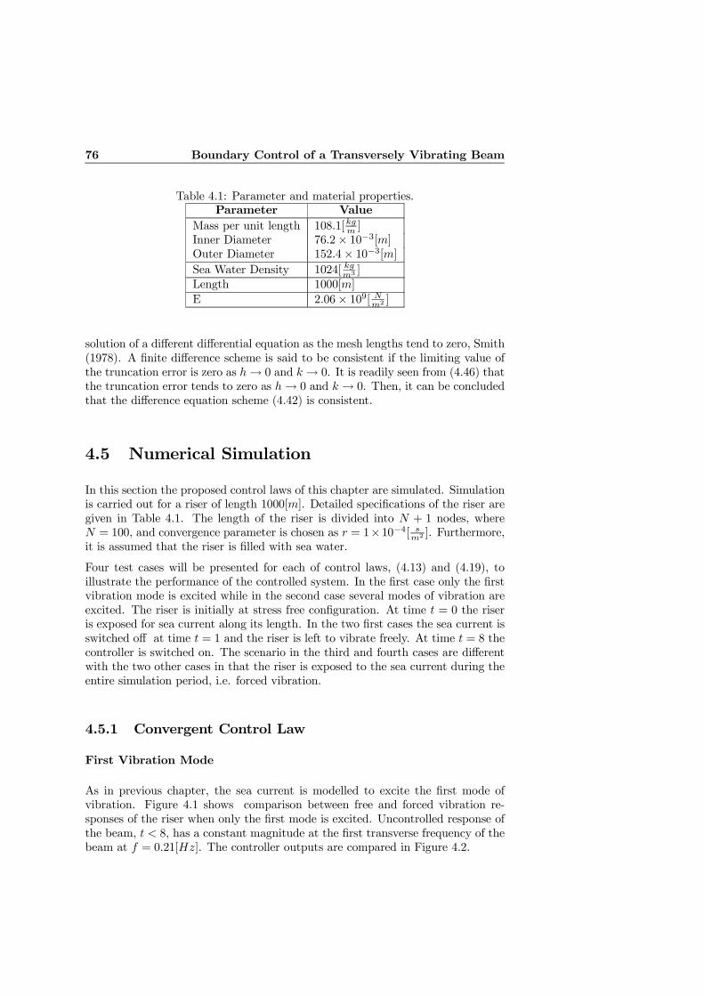
76 Boundary Control of a Transversely Vibrating Beam
Table 4.1: Parameter and material properties.Parameter Value
Mass per unit length 108.1[kgm ]Inner Diameter 76.2× 10⁻³[m]Outer Diameter 152.4× 10⁻³[m]Sea Water Density 1024[ kgm3 ]Length 1000[m]
E 2.06× 10⁹[ Nm2 ]
solution of a different differential equation as the mesh lengths tend to zero, Smith(1978). A finite difference scheme is said to be consistent if the limiting value ofthe truncation error is zero as h→ 0 and k → 0. It is readily seen from (4.46) thatthe truncation error tends to zero as h→ 0 and k → 0. Then, it can be concludedthat the difference equation scheme (4.42) is consistent.
4.5 Numerical Simulation
In this section the proposed control laws of this chapter are simulated. Simulationis carried out for a riser of length 1000[m]. Detailed specifications of the riser aregiven in Table 4.1. The length of the riser is divided into N + 1 nodes, whereN = 100, and convergence parameter is chosen as r = 1×10⁻⁴[ sm2 ]. Furthermore,it is assumed that the riser is filled with sea water.
Four test cases will be presented for each of control laws, (4.13) and (4.19), toillustrate the performance of the controlled system. In the first case only the firstvibration mode is excited while in the second case several modes of vibration areexcited. The riser is initially at stress free configuration. At time t = 0 the riseris exposed for sea current along its length. In the two first cases the sea current isswitched off at time t = 1 and the riser is left to vibrate freely. At time t = 8 thecontroller is switched on. The scenario in the third and fourth cases are differentwith the two other cases in that the riser is exposed to the sea current during theentire simulation period, i.e. forced vibration.
4.5.1 Convergent Control Law
First Vibration Mode
As in previous chapter, the sea current is modelled to excite the first mode ofvibration. Figure 4.1 shows comparison between free and forced vibration re-sponses of the riser when only the first mode is excited. Uncontrolled response ofthe beam, t < 8, has a constant magnitude at the first transverse frequency of thebeam at f = 0.21[Hz]. The controller outputs are compared in Figure 4.2.
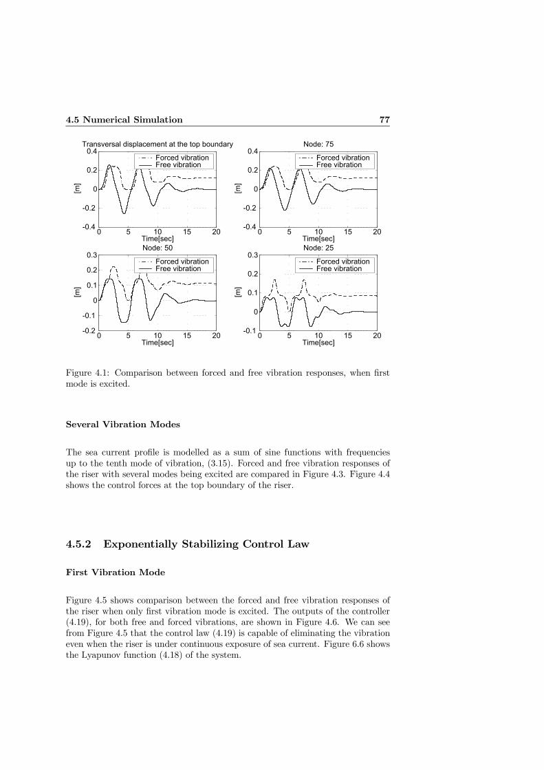
4.5 Numerical Simulation 77
0 5 10 15 20-0.4
-0.2
0
0.2
0.4Transversal displacement at the top boundary
[m]
Time[sec]
Forced vibrationFree vibration
0 5 10 15 20-0.4
-0.2
0
0.2
0.4Node: 75
[m]
Time[sec]
Forced vibrationFree vibration
0 5 10 15 20-0.2
-0.1
0
0.1
0.2
0.3Node: 50
[m]
Time[sec]
Forced vibrationFree vibration
0 5 10 15 20-0.1
0
0.1
0.2
0.3Node: 25
[m]
Time[sec]
Forced vibrationFree vibration
Figure 4.1: Comparison between forced and free vibration responses, when firstmode is excited.
Several Vibration Modes
The sea current profile is modelled as a sum of sine functions with frequenciesup to the tenth mode of vibration, (3.15). Forced and free vibration responses ofthe riser with several modes being excited are compared in Figure 4.3. Figure 4.4shows the control forces at the top boundary of the riser.
4.5.2 Exponentially Stabilizing Control Law
First Vibration Mode
Figure 4.5 shows comparison between the forced and free vibration responses ofthe riser when only first vibration mode is excited. The outputs of the controller(4.19), for both free and forced vibrations, are shown in Figure 4.6. We can seefrom Figure 4.5 that the control law (4.19) is capable of eliminating the vibrationeven when the riser is under continuous exposure of sea current. Figure 6.6 showsthe Lyapunov function (4.18) of the system.
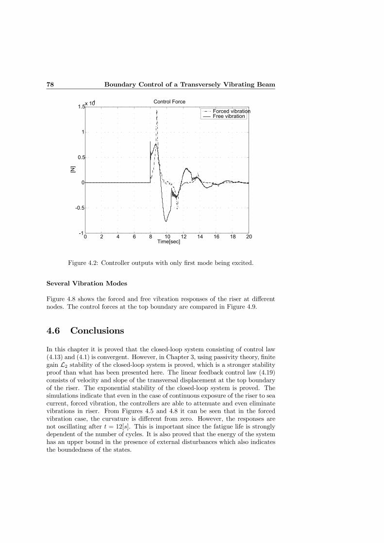
78 Boundary Control of a Transversely Vibrating Beam
0 2 4 6 8 10 12 14 16 18 20-1
-0.5
0
0.5
1
1.5x 10⁴ Control Force
Time[sec]
[N]
Forced vibrationFree vibration
Figure 4.2: Controller outputs with only first mode being excited.
Several Vibration Modes
Figure 4.8 shows the forced and free vibration responses of the riser at differentnodes. The control forces at the top boundary are compared in Figure 4.9.
4.6 Conclusions
In this chapter it is proved that the closed-loop system consisting of control law(4.13) and (4.1) is convergent. However, in Chapter 3, using passivity theory, finitegain L2 stability of the closed-loop system is proved, which is a stronger stabilityproof than what has been presented here. The linear feedback control law (4.19)consists of velocity and slope of the transversal displacement at the top boundaryof the riser. The exponential stability of the closed-loop system is proved. Thesimulations indicate that even in the case of continuous exposure of the riser to seacurrent, forced vibration, the controllers are able to attenuate and even eliminatevibrations in riser. From Figures 4.5 and 4.8 it can be seen that in the forcedvibration case, the curvature is different from zero. However, the responses arenot oscillating after t = 12[s]. This is important since the fatigue life is stronglydependent of the number of cycles. It is also proved that the energy of the systemhas an upper bound in the presence of external disturbances which also indicatesthe boundedness of the states.
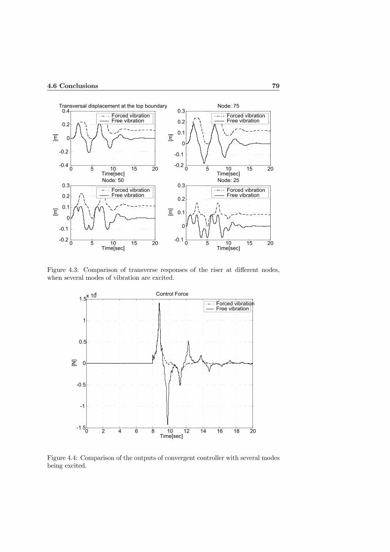
4.6 Conclusions 79
0 5 10 15 20-0.4
-0.2
0
0.2
0.4Transversal displacement at the top boundary
[m]
Time[sec]
Forced vibrationFree vibration
0 5 10 15 20-0.2
-0.1
0
0.1
0.2
0.3Node: 75
[m]
Time[sec]
Forced vibrationFree vibration
0 5 10 15 20-0.2
-0.1
0
0.1
0.2
0.3Node: 50
[m]
Time[sec]
Forced vibrationFree vibration
0 5 10 15 20-0.1
0
0.1
0.2
0.3Node: 25
[m]
Time[sec]
Forced vibrationFree vibration
Figure 4.3: Comparison of transverse responses of the riser at different nodes,when several modes of vibration are excited.
0 2 4 6 8 10 12 14 16 18 20-1.5
-1
-0.5
0
0.5
1
1.5x 10⁴ Control Force
Time[sec]
[N]
Forced vibrationFree vibration
Figure 4.4: Comparison of the outputs of convergent controller with several modesbeing excited.
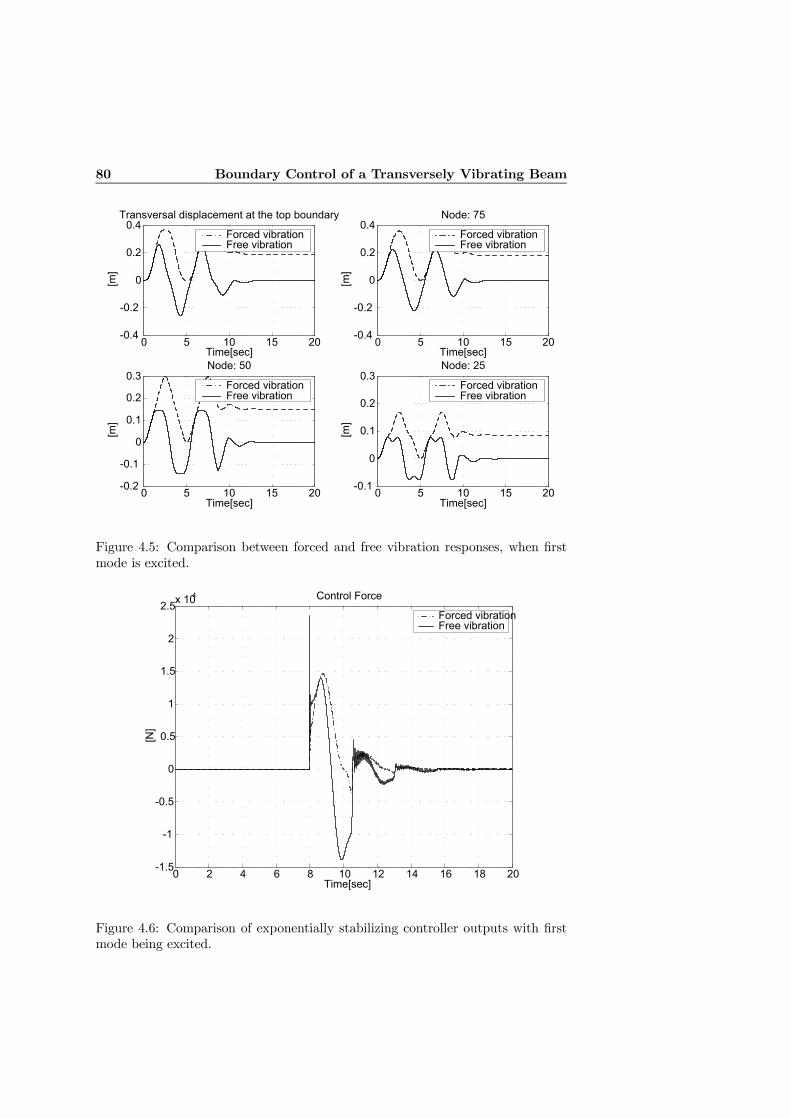
80 Boundary Control of a Transversely Vibrating Beam
0 5 10 15 20-0.4
-0.2
0
0.2
0.4Transversal displacement at the top boundary
[m]
Time[sec]
Forced vibrationFree vibration
0 5 10 15 20-0.4
-0.2
0
0.2
0.4Node: 75
[m]
Time[sec]
Forced vibrationFree vibration
0 5 10 15 20-0.2
-0.1
0
0.1
0.2
0.3Node: 50
[m]
Time[sec]
Forced vibrationFree vibration
0 5 10 15 20-0.1
0
0.1
0.2
0.3Node: 25
[m]
Time[sec]
Forced vibrationFree vibration
Figure 4.5: Comparison between forced and free vibration responses, when firstmode is excited.
0 2 4 6 8 10 12 14 16 18 20-1.5
-1
-0.5
0
0.5
1
1.5
2
2.5x 10⁴ Control Force
Time[sec]
[N]
Forced vibrationFree vibration
Figure 4.6: Comparison of exponentially stabilizing controller outputs with firstmode being excited.
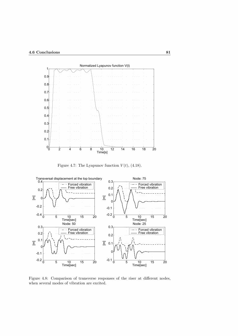
4.6 Conclusions 81
0 2 4 6 8 10 12 14 16 18 200
0.1
0.2
0.3
0.4
0.5
0.6
0.7
0.8
0.9
1Normalized Lyapunov function V(t)
Time[s]
Figure 4.7: The Lyapunov function V (t), (4.18).
0 5 10 15 20-0.4
-0.2
0
0.2
0.4Transversal displacement at the top boundary
[m]
Time[sec]
Forced vibrationFree vibration
0 5 10 15 20-0.2
-0.1
0
0.1
0.2
0.3Node: 75
[m]
Time[sec]
Forced vibrationFree vibration
0 5 10 15 20-0.2
-0.1
0
0.1
0.2
0.3Node: 50
[m]
Time[sec]
Forced vibrationFree vibration
0 5 10 15 20-0.1
0
0.1
0.2
0.3Node: 25
[m]
Time[sec]
Forced vibrationFree vibration
Figure 4.8: Comparison of transverse responses of the riser at different nodes,when several modes of vibration are excited.
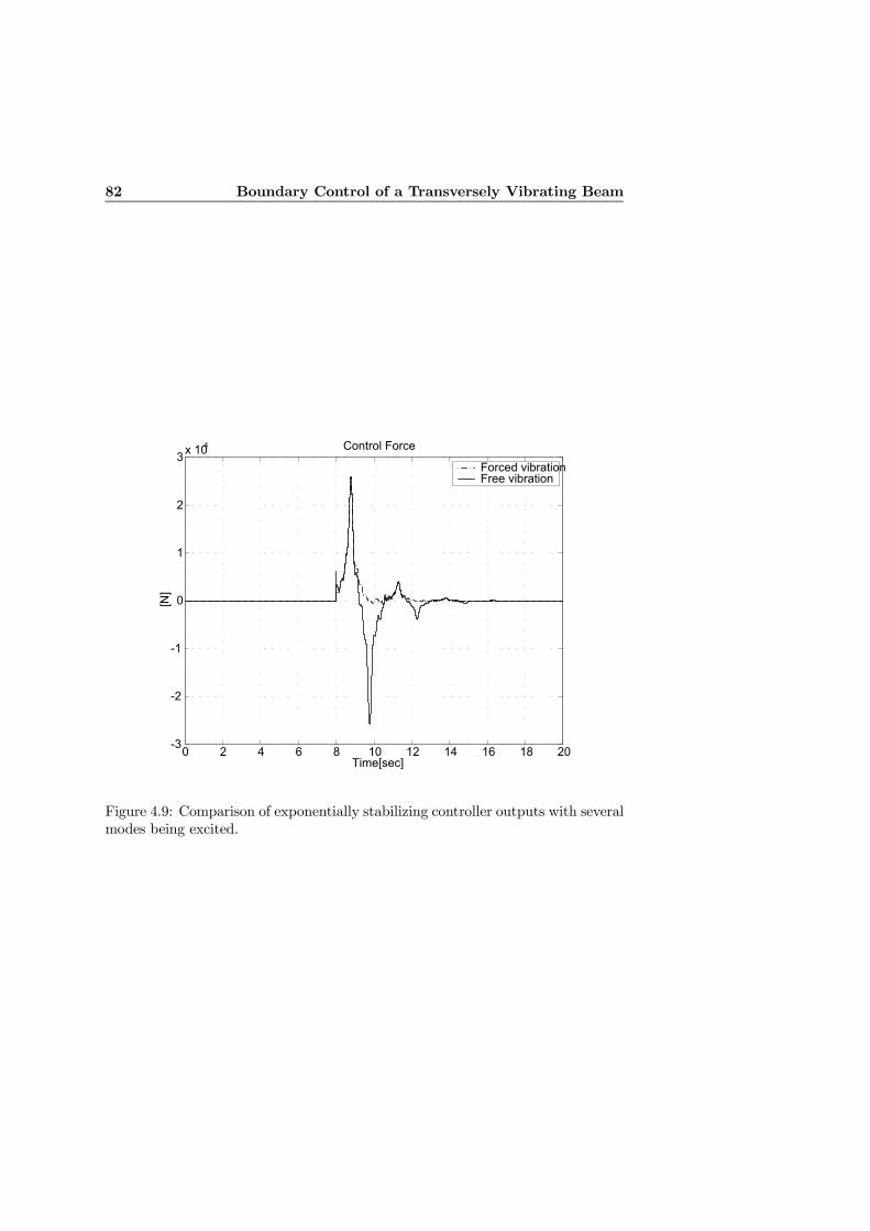
82 Boundary Control of a Transversely Vibrating Beam
0 2 4 6 8 10 12 14 16 18 20-3
-2
-1
0
1
2
3x 10⁴ Control Force
Time[sec]
[N]
Forced vibrationFree vibration
Figure 4.9: Comparison of exponentially stabilizing controller outputs with severalmodes being excited.
Chapter 5
Boundary Control of aCoupled Nonlinear Beam
In previous chapter we focused on the transverse dynamics of a vibrating beam. Inthis chapter a coupled nonlinear model for beams is considered. Coupling betweenlongitudinal and transverse dynamic is due to the fact that the effect of axialelongation are taken into account. Control laws will be designed to guaranteeconvergent and exponential stability of states of the underlying system. Some ofthe results of this chapter have been presented in Fard & Sagatun (2000b).
5.1 Equations of Motion
The mathematical model derived in Chapter 2, (2.39)-(2.40), for a coupled, non-linear beam as shown in Figure (2.7) will be considered. The equations of motionare restated here for convenience.
ρAηtt(x, t) +EIηxxxx(x, t)− P0ηxx(x, t)−3
2EAη2x(x, t)ηxx(x, t)
−EAηxx(x, t)µx(x, t)−EAηx(x, t)µxx(x, t)− f(x, t) = 0 (5.1a)
ρAµtt(x, t)−EAηx(x, t)ηxx(x, t)−EAµxx(x, t) = 0 (5.1b)
∀ (x, t) ∈ (0, L)× [0,∞). Note that (2.28) will give the same equations of motion,when the axial strain-displacement relationship is given by
P (x, t) = P0 +1
2EAη2x(x, t) +EAµx(x, t). (5.2)
Equation (5.2) indicates that tension, P (x, t), is due to the constant axial force,force due to bending in the beam and force resulting from elongation of the beam.Note that P (x, t) is also a function of the second independent variable, x, whichindicates that the tension varies along the length of the beam.
84 Boundary Control of a Coupled Nonlinear Beam
The boundary conditions for a simply supported beam, as shown in Figure (2.7),are given as
η(0, t) = η(L, t) = 0 (5.3a)
EIηxx(0, t) = EIηxx(L, t) = 0 (5.3b)
µ(0, t) = 0 (5.3c)
u(t) =1
2EAη2x(L, t) +EAµx(L, t). (5.3d)
Boundary condition (5.3d) represents force balance at the boundary x = L, andu(t) is the control force at the boundary. The initial conditions are
η(x, 0) = g1(x) (5.4)
ηt(x, 0) = g2(x) (5.5)
µ(x, 0) = g3(x) (5.6)
µt(x, 0) = g4(x) (5.7)
∀ x ∈ (0, L). Equations (5.4)-(5.7) denote the initial transverse and longitudinalposition and velocity functions.
5.1.1 Assumptions
Assumption 5.1 It will be assumed that
1. P (x, t) − P0 ≥ 0 for all (x, t) ∈ [0, L] × [0,∞). This implies that the beamis not exposed to compression at any point. This is a practical and requiredproperty.
2. there exists a solution for the dynamics given by (5.1a)-(5.1b) and (5.3a)-(5.3d). It is also assumed that the displacements η(x, t), µ(x, t) and itstime derivative ηt(x, t), µt(x, t) belong to a space of function which has thefollowing properties:
i) If the potential energy of the system is proved to be bounded ∀t ∈ [0,∞),then ∂nη(x,t)
∂xn and ∂mµ(x,t)∂xm are bounded for n = 3, 4, m = 2, ∀(x, t) ∈
[0, L]× [0,∞) andii) If the kinetic energy of the system is proved to be bounded ∀t ∈ [0,∞),
then ∂nηt(x,t)∂xn and ∂mµt(x,t)
∂xm are bounded for n = m = 1, and ∀(x, t) ∈[0, L]× [0,∞).
5.2 Design of Boundary Control Laws
The discussion in this section will be limited to free vibration of beams; hence,f(x, t) = 0 for t > 0. In addition to the results from Lemma 4.1, some moreidentities will be proved in the following. These identities will be used in thesubsequent stability analysis.
5.2 Design of Boundary Control Laws 85
Lemma 5.1 Let η(x, t) and µ(x, t) be solutions of (5.1a)-(5.1b) which satisfy theboundary conditions (5.3a)-(5.3d). Then
EA
Z L
0
(µxµxt + µxxµt) dx = EA µxµt|L0 (5.8)
γρA
Z L
0
xµtµxtdx = γρA
"L
2µ2t (L, t)−
1
2
Z L
0
µ2tdx
#(5.9)
γEA
Z L
0
xµxxµxdx = γEA
"L
2µ2x(L, t)−
1
2
Z L
0
µ2xdx
#(5.10)
EA
Z L
0
ηxxµxηtdx+EA
Z L
0
ηxµxxηtdx+EA
Z L
0
ηxηxxµtdx+ γEA
Z L
0
xη2xµxxdx
+EA
Z L
0
ηxηxtµxdx+EA
2
Z L
0
η2xµxtdx+ 2γEA
Z L
0
xηxxµxηxdx
= EA ηxµxηt|L0 + γEALη2x (L, t)µx (L, t) +EA1
2η2xµt
¯L0
− γEA
Z L
0
η2xµxdx
(5.11)
∀ t ≥ 0.
Proof : See Appendix B¥.
5.2.1 Convergent Controller
Consider the Lyapunov functional
V (t) =ρA
2
Z L
0
η2t (x, t)dx+P02
Z L
0
η2x(x, t)dx+EI
2
Z L
0
η2xx(x, t)dx
+ρA
2
Z L
0
µ2t (x, t)dx+EA
2
Z L
0
µµx(x, t) +
1
2η2x(x, t)
¶2dx (5.12)
where η(x, t) and µ(x, t) satisfy the boundary value-problem (5.1a)-(5.1b) and(5.3a)-(5.3d). Equation (5.12) represents the mechanical energy of the system.
Theorem 5.1 Let the boundary control law u(t) in (5.3d) be
u(t) = −Kµt(L, t) (5.13)
where K > 0. Then, the functional V (t) along the solution of the system (5.1a)-(5.1b), with corresponding boundary conditions, (5.3a)-(5.3d), satisfies
V (t) = −Kµt(L, t)2. (5.14)
Hence, the states of the system, ηt(x, t), ηx(x, t), ηxx(x, t), µt(x, t), η2x(x, t) +
µx(x, t), µ(x, t) and η(x, t) are bounded and converge to zero.
86 Boundary Control of a Coupled Nonlinear Beam
Proof: The time derivative of the functional V (t), (5.12), is given by
V (t) = ρA
Z L
0
ηtηttdx+ P0
Z L
0
ηxηxtdx+EI
Z L
0
ηxxηxxtdx
+ρA
Z L
0
µtµttdx+EA
Z L
0
µµx +
1
2η2x
¶(µxt + ηxηxt) dx.
After substitution of ρAηtt and ρAµtt from (5.1a)-(5.1b) we obtain
V (t) =
Z L
0
·−EIηxxxx + P0ηxx +
3
2EAη2xηxx +EAηxxµx +EAηxµxx
¸ηtdx
+P0
Z L
0
ηxηxtdx+EI
Z L
0
ηxxηxxtdx+
Z L
0
[EAµxx +EAηxηxx]µtdx
+EA
Z L
0
µxµxtdx+EA
Z L
0
µxηxηxtdx+EA
2
Z L
0
η2xµxtdx.+EA
2
Z L
0
η3xηxtdx.
The results from lemmas 4.1 and 5.1 are combined with the boundary conditions(5.3a)-(5.3d) to obtain
V (t) =
µEAµx(L, t) +EA
1
2η2x(L, t)
¶µt(L, t).
Note that the boundary condition (5.3a) is used to conclude that ηt(x, t) = 0 forx = 0, L. Using boundary control law (5.13) we get (5.14). By results so far, itcan be concluded that the total mechanical energy, V (t), is bounded and remainsbounded ∀ t ≥ 0.Due to boundedness of potential energy, we use property i of Assumption 5.1 toconclude that ∂nη(x,t)
∂xn and ∂mµ(x,t)∂xm are bounded for n = 3, 4, m = 2, and ∀(x, t) ∈
[0, L]× [0,∞) . Furthermore, by using property ii of Assumption 5.1 we concludethat ∂
nηt(x,t)∂xn and ∂mµt(x,t)
∂xm are bounded for n =m = 1, and ∀(x, t) ∈ [0, L]×[0,∞).To prove convergence of states we have to establish that V (t) is uniformly con-tinuous. A sufficient condition for V (t) to be uniformly continuous is that itsderivative V (t) is bounded ∀t ≥ 0, Fossen (1994). The derivative of (5.14) withrespect to time is given by
V (t) = −Kµt(L, t)µtt(L, t).It has been established that ηt(x, t) is bounded ∀(x, t) ∈ [0, L]× [0,∞). Equationsof motion (5.1a)-(5.1b) and the boundedness of ∂nη(x,t)
∂xn and ∂mµ(x,t)∂xm for respec-
tively n = 3, 4, m = 2, may be used to show that µtt(x, t) and ηtt(x, t) are bounded∀(x, t) ∈ (0, L)× [0,∞).Time derivative of boundary condition (5.3d) after substitution of control law(5.13) is
−Kµtt(L, t) = EAµxt(L, t) +EAηx(L, t)ηxt(L, t) (5.15)
5.2 Design of Boundary Control Laws 87
We use (5.15) and boundedness of ∂nηt(x,t)∂xn and ∂mµt(x,t)
∂xm for n = m = 1 toconclude boundedness of µtt(L, t) for all t ≥ 0. Hence, according to Barbalat’slemma, Barbâlat (1959), V (t) → 0 as t → ∞. Hence, the states of the systemconverge to zero as t → ∞. Now due to the boundary conditions (5.3a) and thefact that state vector, q(t), converges to zero, we can conclude that η(x, t) convergeto zero as t→ 0.¥
5.2.2 Exponentially Stabilizing Control Law
The following Lyapunov functional is introduced:
V (t) = ρ(q,0)2 + γρA
Z L
0
xηt(x, t)ηx(x, t)dx
+γρA
Z L
0
xµt(x, t)µx(x, t)dx ∀t ≥ 0 (5.16)
where γ is a small positive constant real number and the metric ρ(q,0) is definedas
ρ(q,0) =
"ρA
2
Z L
0
η2t (x, t)dx+P02
Z L
0
η2x(x, t)dx +EA
8
Z L
0
η4x(x, t)dx
+EI
2
Z L
0
η2xx(x, t)dx+ρA
2
Z L
0
µ2t (x, t)dx+EA
2
Z L
0
µ2x(x, t)dx
+EA
2
Z L
0
η2x(x, t)µx(x, t)dx
# 12
(5.17)
The metric ρ(q,0) establishes a measure of closeness of the state qT= [ηt, ηx, ηxx, µt,¡η2x + µx
¢]T to the equilibrium null state in terms of the velocity, slope and cur-
vature of transversal displacement and slope and velocity of longitudinal displace-ment of the beam. Furthermore, if ρ(q,0) is small, then each of its terms mustthen also be small, as the integrand of ρ(q,0) is the sum of these non-negativeterms. The metric ρ(q,0) may also be considered a measure of the total energyof the system.
Theorem 5.2 Let the boundary control law u(t) in (5.3d) be:
u(t) = −(EA)2
P0
µK1Lγµx(L, t)µt(L, t) +
K22Lγ
η2x(L, t)µt(L, t)
−K3 P0EA
µx(L, t) +3
8K4η
4x(L, t) +K5
ρ
2Eµ2t (L, t)
+K62µ2x(L, t) +K7η
2x (L, t)µx (L, t)
¶(5.18)
88 Boundary Control of a Coupled Nonlinear Beam
where feedback gains are selected according to
0 ≤ K1 ≤ 1 , 0 ≤ K2 ≤ 1K3 = 1,K4 ≥ 4
3K7
K5 ≥ 1, K6 ≥ 10 ≤ K7 ≤ 1. (5.19)
Then, the functional V (t) along the solution of the distributed parameter dynamicsystem, (5.1a)-(5.1b) with corresponding boundary conditions (5.3a)-(5.3d), satis-fies
V (t) ≤ V (0) expµ− γ
(1 + γγ1)
¶t. (5.20)
Furthermore,
ρ(q,0) ≤s1 + γγ11− γγ1
ρ(q (0) ,0) exp
µ− γ
2(1 + γγ1)
¶t (5.21)
where γ1 = Lmax³1, ρAP0 ,
ρE
´. Hence, the states of the system tends to zero expo-
nentially.
To prove the Theorem 5.2 it is necessary to establish the following lemma.
Lemma 5.2 Let γ in (5.16) satisfy
γ ¿ 1
γ1. (5.22)
Then, the functional V (t) satisfies the following inequality
(1− γγ1) ρ2(q, 0) ≤ V (t) ≤ (1 + γγ1) ρ
2(q, 0) (5.23)
∀ t ≥ 0. Furthermore, V (t) is positive definite with respect to metric ρ(q,0) andadmits an infinitesimally upper limit.
Proof : The following inequality is valid:
5.2 Design of Boundary Control Laws 89
ρA
Z L
0
xηt(x, t)ηx(x, t)dx+ ρA
Z L
0
xµt(x, t)µx(x, t)dx
≤ ρA
Z L
0
x |ηt(x, t)| |ηx(x, t)|dx+ ρA
Z L
0
x |µt(x, t)| |µx(x, t)| dx
≤ ρAL
2
Z L
0
η2x(x, t)dx+ρAL
2
Z L
0
η2t (x, t)dx
+ρAL
2
Z L
0
µ2x(x, t)dx+ρAL
2
Z L
0
µ2t (x, t)dx
= L
"ρA
P0
P02
Z L
0
η2x(x, t)dx+ρA
2
Z L
0
η2t (x, t)dx
+ρA
2
Z L
0
µ2t (x, t)dx+ρ
E
EA
2
Z L
0
µ2x(x, t)dx
#
≤ Lmax
µ1,ρA
P0,ρ
E
¶ρ2(q, 0)
≤ γ1ρ2(q, 0)
∀ t ≥ 0, where the second inequality is obtained using the following inequality
|ηt(x, t)| |ηx(x, t)| ≤1
2
¡η2t (x, t) + η2x(x, t)
¢.
In a similar way the left side of the inequality (5.23) can be proved. It is clearfrom the definition of the metric ρ(q, 0), (5.17), that ρ(q, 0) is positive definite;hence, from inequality (5.23) and with γ satisfying the inequality (5.22), it isconcluded that the functional V (t) is also positive definite. The right-hand side ofthe inequality (5.23) indicates that the functional V (t) has an upper limit whichis given by (1 + γγ1) ρ
2(q, 0).¥Time derivative of the functional V (t) after substitution of ρAηtt(x, t) and ρAµtt(x, t)from (5.1a)-(5.1b) is given by
V (t) =
Z L
0
·−EIηxxxx + P0ηxx +
3
2EAη2xηxx +EAηxxµx +EAηxµxx
¸ηtdx
+P0
Z L
0
ηxηxtdx+EA
2
Z L
0
η3xηxtdx+EI
Z L
0
ηxxηxxtdx+EA
Z L
0
µxµxtdx
+
Z L
0
[EAµxx +EAηxηxx]µtdx+EA
Z L
0
ηxηxtµxdx+EA
2
Z L
0
η2xµxtdx
+γ
Z L
0
x
·−EIηxxxx + P0ηxx +
3
2EAη2xηxx +EAηxxµx +EAηxµxx
¸ηxdx
+γρA
Z L
0
xηtηxtdx+ γ
Z L
0
x [EAµxx +EAηxηxx]µxdx+ γρA
Z L
0
xµtµxtdx.
90 Boundary Control of a Coupled Nonlinear Beam
Using results from lemmas 4.1 and 5.1, and
EAµx(x, t) = P (x, t)− P0 −1
2EAη2x(x, t)
from strain-displacement relationship, (5.2), we have
V (t) = −γρ2(q,0)− γEI
Z L
0
η2xxdx−1
2γ
Z L
0
(P (x, t)− P0)η2xdx
−EI ηxxxηt|L0 +EI ηxxηtx|L0 +EA
2η3xηt
¯L0+EA µxµt|L0 + P0 ηxηt|L0
+EA ηxµxηt|L0 +EA1
2η2xµt
¯L0
+ γL
2P0η
2x(L, t) + γ
3L
8EAη4x(L, t)
+γρAL
2η2t (L, t) + γρA
L
2µ2t (L, t) + γEA
L
2µ2x(L, t) + γEALη2x (L, t)µx (L, t) .
Proof of Theorem 5.2: Applying the boundary conditions (5.3a)-(5.3d) withthe control law u(t) as in (5.18), under the Assumption 5.1, we obtain
V (t) = −γρ2(q,0)− γP 20L
EA−EA (K1 − 1)µx(L, t)µt(L, t)
−12EA (K2 − 1) η2x(L, t)µt(L, t)− γP0L (1−K3)µx(L, t)
−38γLEA (K4 − 1) η4x(L, t)− γL
ρA
2(K5 − 1)µ2t (L, t)
−γEAL2(K6 − 1)µ2x(L, t)− γLEA (K7 − 1) η2x (L, t)µx (L, t) .
By using the following inequalities
µx(L, t)µt(L, t) ≥ −12µx(L, t)
2 − 12µt(L, t)
2
η2x(L, t)µt(L, t) ≥ −12η4x(L, t)−
1
2µt(L, t)
2
η2x(L, t)µx(L, t) ≥ −12η4x(L, t)−
1
2µx(L, t)
2
the expression for V (t) can be written as
V (t) ≤ −γρ2(q,0)− γP 20L
EA
−·EA
2(1−K1) + γ
LEA
2(1−K7) + γ
EAL
2(K6 − 1)
¸µ2x(L, t)
−·EA
2(1−K1) + γ
LρA
2(K5 − 1) + EA
4(1−K2)
¸µt(L, t)
2
−·EA
4(1−K2) + γ
LEA
2
µ3
4K4 −K7
¶+LEA
8γ
¸η4x(L, t)
−γP0L (1−K3)µx(L, t).
5.3 External Disturbances 91
Now choosing the control gains according to (5.19) the following expression fortime derivative of the functional V (t) is obtained
V (t) ≤ −γρ2(q,0).
Using the inequality (5.23) we get
V (t) ≤ − γ
(1 + γγ1)V (t).
By the comparison lemma Khalil (1996) the inequality (5.20) is proved. From(5.20), using the inequalities (5.22) and (5.23) we obtain
ρ(q,0) ≤ ρ(q,0) ≤s1 + γγ11− γγ1
ρ(q (0) ,0) exp
µ− γ
2(1 + γγ1)
¶t
which is the inequality (5.21).
Since the metric ρ(q,0) is positive definite and tends to zero exponentially, it isclear that each of its terms must tend to zero exponentially. This means that ηt,ηx, ηxx, µt and
¡η2x + µx
¢ → 0 exponentially as t → ∞ for all x ∈ [0, L]. Sinceη2x(x, t)→ 0 exponentially so does the µx(x, t).
ηx(x, t) → 0 exponentially as t → ∞ for all x ∈ [0, L]. Since η(x, t) = 0 forx = 0, L and ∀ t ≥ 0, according to the boundary condition (5.3a), we concludethat η(x, t) → 0 exponentially as t → ∞ for all x ∈ [0, L]. Since µx(x, t) →0 exponentially as t → ∞ for all x ∈ [0, L] and due to the boundary condition(5.3c) we can conclude that µ(x, t) tends to its initial state.¥
Remark 5.1 Note that µx(x, t) represents the dynamic strain. Since the beamis pretensioned, it possesses a static strain and displacement. The theorem con-cludes that the dynamic strain tends to zero; hence, the beam retrieves its initialconfiguration at the steady state.
5.3 External Disturbances
So far only the free vibration, f(x, t) = 0 for t > 0, has been considered. As inSection 4.3 a bound on the metric ρ(q,0), (5.17) can be established for forcedvibration, i.e. f(x, t) 6= 0 for t ≥ 0.
Lemma 5.3 Let q = 0 be the exponentially stable equilibrium of the nominalsystem,(5.1a)-(5.1b) and (5.3a)-(5.3d) with the control law (5.18) and f(x, t) =0,∀t > 0, and the control law (5.18). Suppose the perturbation f(x, t) satisfies
kf(x, t)kL2 = β(t)ρ(q,0) + δ(t) ∀t ≥ 0 (5.24)
92 Boundary Control of a Coupled Nonlinear Beam
in the neighborhood Sr of q = 0, where β : R→ R is nonnegative and continuous∀ t ≥ 0 and satisfiesZ t
t0
β(τ)dτ ≤ ε(t− t0) + ξ ε <γ (1− γγ1)
C (1 + γγ1)(5.25)
where ε and n are nonnegative constants and δ : R → R is nonnegative, contin-uous, and bounded ∀ t ≥ 0. Furthermore, γ1 = Lmax
³1, ρAP0 ,
ρE
´and γ satisfies
the (5.22). Then, if the conditions
ρ(q(t0),0) <r
eC
2(1−γγ1) ξ
s(1− γγ1)
(1 + γγ1)(5.26)
supt≥t0
δ(t) <2α(1− γγ1)
CeC
2(1−γγ1) ξr (5.27)
are satisfied, a bound for ρ(q,0) is obtained as:
ρ(q,0) ≤s(1 + γγ1)
(1− γγ1)e
C2(1−γγ1) ξρ(q(t0),0)e
−α(t−t0)
+C
2p(1− γγ1)
eC
2(1−γγ1) ξZ t
t0
e−α(t−τ)δ(τ)dτ . (5.28)
Proof: The proof is the same as the proof of Lemma 4.3 and will not be repeatedhere.
5.4 Conclusions
Coupled nonlinear equations of a beam are studied in this chapter. Two controllershave been designed for the nonlinear beam. A linear control law using feedbackfrom velocity of the beam at its boundary guarantees convergent of the states. Thisis proved by Barbalat’s lemma. Another control law ensures exponentially stabilityof the states. The control law in (5.18) is complicated in structure. However, it iseasy and inexpensive to implement due to the fact that all states in the controllerare measured or observed directly. µx(L, t) is measured directly by a strain gaugelocated on the top boundary of the beam. µt(L, t) may be estimated throughposition measurements of the end position of the beam. The transverse slope,ηx(L, t), can be directly measured by using inclinometers.
Chapter 6
Numerical Simulation ofCoupled Dynamic
Performance of proposed control laws will be tested in this chapter. Numericalanalysis of the nonlinear coupled equations of motion and the control law (5.18)will be carried out, using finite difference methods.
6.1 Nondimensional Formulation
In the following study it is convenient to transform the equations of motion (5.1a)-(5.1b) into nondimensional form. The nondimensional variables (4.38a)-(4.38c)will be used here. For the second independent variable, time, the following nondi-mensional variable is introduced:
τ =1
L2
sEI
ρAt⇒ t = L2
rρA
EIτ = ατ
where τ is the nondimensional time. Substitution of these variables into the (5.1a)-(5.1b), dropping the asterisks, the nondimensional equations of motion are ob-tained as
ηττ (x, τ) = −a1ηxxxx(x, τ) + a2ηxx(x, τ) +3
2a3η
2x(x, τ)ηxx(x, τ)
+a3ηxx(x, τ)µx(x, τ) + a3ηx(x, τ)µxx(x, τ) + a4f(x, τ) (6.1a)
µττ (x, τ) = a3ηx(x, τ)ηxx(x, τ) + a3µxx(x, τ), (6.1b)
94 Numerical Simulation of Coupled Dynamic
where the coefficients are given as
a1 =EIα2
ρAL4
a2 =P0α
2
ρAL2
a3 =Eα2
ρL2
a4 =α2
ρAL.
Boundary conditions can also be expressed in this form as
ηxx(0, τ) = ηxx(1, τ) = 0
η(0, τ) = η(1, τ) = 0
µ(0, τ) = 0
u(τ) =1
2η2x(1, τ) + µx(1, τ)
where u(t) = EAu(τ).
6.2 Discretization using Finite DifferenceMethod
It is assumed that the domain to be examined is covered by uniform rectangulargrid with sides parallel to the x- and t-axes, with h and k being the grid spacingsin the x- and t-directions respectively. Furthermore, it is assumed that the pointconsidered is the point x = ih and τ = jk of the domain, where i and j areintegers and i = j = 0 is the origin. The value of functions η(., .), ηx(., .), µ(., .)and P (., .) at the point x = ih and τ = jk are denoted by ηij , ηxi,j , µi,j and Pij .The following approximations for partial derivatives are used:µ
∂4η
∂x4
¶i,j
=ηi+2,j − 4ηi+1,j + 6ηi,j − 4ηi−1,j + ηi−2,j
h4+O(h2) (6.2a)µ
∂2η
∂x2
¶i,j
=ηi+1,j − 2ηi,j + ηi−1,j
h2+O(h2) (6.2b)µ
∂η
∂x
¶i,j
=ηi+1,j − ηi,j
h+O(h2) (6.2c)µ
∂2η
∂τ2
¶i,j
=ηi,j+1 − 2ηi,j + ηi,j−1
k2+O(k2) (6.2d)
Same approximations for derivatives of µ(x, τ) are applied. Using these approxi-mation, the finite difference scheme for (6.1a)-(6.1b) takes the form
6.2 Discretization using Finite Difference Method 95
ηi,j+1 = 2ηi,j − ηi,j−1 − a1r2¡ηi+2,j − 4ηi+1,j + 6ηi,j − 4ηi−1,j + ηi−2,j
¢+a2r
2h2¡ηi+1,j − 2ηi,j + ηi−1,j
¢+3
2a3r
2h2η2xi,j¡ηi+1,j − 2ηi,j + ηi−1,j
¢+a3r
2h¡ηi+1,j − 2ηi,j + ηi−1,j
¢ ¡µi+1,j − µi,j
¢+a3r
2h2ηxi,j¡µi+1,j − 2µi,j + µi−1,j
¢+ a4k
2fi,j (6.3a)
µi,j+1 = 2µi,j − µi,j−1 + a3r2h2ηxi,j¡ηi+1,j − 2ηi,j + ηi−1,j
¢+a3r
2h2¡µi+1,j − 2µi,j + µi−1,j
¢(6.3b)
where the convergence parameter, r, is defined as r = kh2 .
6.2.1 Truncation Error and Consistency
By Taylor’s Theorem, it can be proved that the principal part of truncation errorsfor the scheme (6.3a)-(6.3b) are given by
eηi,j = −k2
12(ηττττ )i,j + a2
µh2
12(ηxxxx)i,j +O(h
3)
¶+1
8a3h
2η2xi,j (ηxxxx)i,j + a3
µh2
12(ηxxxx)i,j (µx)i,j +
h3
24(ηxxxx)i,j (µxx)i,j
+h4
72(ηxxxx)i,j (µxxx)i,j +
h5
288(ηxxxx)i,j (µxxxx)i,j +
h
2(µxx)i,j (ηxx)i,j
+h2
6(µxxx)i,j (ηxx)i,j +
h3
24(µxxxx)i,j (ηxx)i,j
¶+ a3
h2
12ηxi,j (µxxxx)i,j (6.4)
and
eµi,j =h2
12a3ηxi,j (ηxxxx)i,j +
h2
12a3 (µxxxx)i,j
−k2
12(µττττ )i,j +O(k
3) +O(h3). (6.5)
It is clear from (6.4) and (6.5) that truncation errors have the order O(h+k2) andO(h2+k2), respectively. Hence, it can be concluded that the scheme (6.3a)-(6.3b)is consistent since the truncation errors tend to zero as h→ 0 and k → 0.
96 Numerical Simulation of Coupled Dynamic
6.3 Numerical Analysis of the Control Law
The control law (5.18) is transformed into the nondimensional form and discreti-cized using the same approximation as for the equations of the motion.
u(τ) = −EAP0
£b1µxµτ + b2η
2xµτ − b3µx + b4η4x + b5µ2τ + b6µ2x + b7η2xµx
¤= −EA
P0
·b1hk
¡µi+1,j − µi,j
¢ ¡µi,j+1 − µi,j
¢+b2h2k
¡ηi+1,j − ηi,j
¢2 ¡µi,j+1 − µi,j
¢−b3h
¡µi+1,j − µi,j
¢+b4h4¡ηi+1,j − ηi,j
¢4+b5k2¡µi,j+1 − µi,j
¢2+b6h2¡µi+1,j − µi,j
¢2+b7h3¡ηi+1,j − ηi,j
¢2 ¡µi+1,j − µi,j
¢¸(6.6)
where the coefficients are given as
b =h
K1
γαK2
2γα K3P0EA
38K4 K5
ρL2
2Eα2K6
2 K7
i.
6.3.1 Truncation Error and Consistency of the Control Law
Using Taylor’s expansion up to the second order for the involving terms in the(6.6) we get
u(τ) = −EAP0
£b1µxµτ + b2η
2xµτ − b3µx + b4η4x + b5µ2τ + b6µ2x + b7η2xµx
¤= −EA
P0
·b1hk
µh (µx)i,j +
h2
2(µxx)i,j
¶µk (µτ )i,j +
k2
2(µττ )i,j
¶+b2h2k
µh (ηx)i,j +
h2
2(ηxx)i,j
¶2µk (µτ )i,j +
k2
2(µττ )i,j
¶−b3h
µh (µx)i,j +
h2
2(µxx)i,j
¶+b4h4
µh (ηx)i,j +
h2
2(ηxx)i,j
¶4+b5k2
µk (µτ )i,j +
k2
2(µττ )i,j
¶2+b6h2
µh (µx)i,j +
h2
2(µxx)i,j
¶2+b7h3
µh (ηx)i,j +
h2
2(ηxx)i,j +O(h
3)
¶2µh (µx)i,j +
h2
2(µxx)i,j +O(h
3)
¶¸.
6.4 Numerical Simulation 97
Table 6.1: Parameter and material properties.Parameter ValueMass per unit length 108.1[kgm ]Inner diameter 76.2× 10⁻³[m]Outer diameter 152.4× 10⁻³[m]Sea water density 1024[ kgm3 ]Length 100[m]
E 2.15× 10¹⁰[ Nm2 ]
After some manipulation the control law’s truncation error is found to be
ebi,j = b1k
2
³(µx)i,j
´(µττ )i,j +
b12(µxx)i,j
µk (µτ )i,j +
k2
2(µττ )i,j
¶+b2
µh2
4(ηxx)
2i,j + h
1 (ηx)i,j (ηxx)i,j
¶µ(µτ )i,j +
k
2(µττ )i,j
¶+b2
k
2(ηx)
2i,j (µττ )i,j +O(h
6k3)− b3h2(µxx)i,j
+b4
µ2h (ηxx)i,j (ηx)
3i,j + 3
h2
2(ηxx)
2i,j (ηx)
2i,j
h3
2(ηxx)
3i,j (ηx)i,j +
1
16(ηxx)
4i,j
¶+b5
µk2
4(µττ )
2i,j + k
1 (µτ )i,j (µττ )i,j
¶+b6
h2
4(µxx)
2i,j + b6h (µx)i,j (µxx)i,j
+b7
µh
4(ηxx)
2i,j + (ηx)i,j (ηxx)i,j
¶µh (µx)i,j +
h2
2(µxx)i,j
¶+b7
h
2(ηx)
2i,j (µxx)i,j
which is of order O(h + k). It is easy to see that the truncation error for thecontrol law tends to zero as h→ 0 and k → 0. This is to conclude that the finitedifference scheme for control law, (6.6), is consistent.
6.4 Numerical Simulation
In this section the proposed control laws of previous chapter are simulated. Nu-merical simulations are carried out for a marine riser of length 100[m]. Detailedspecifications of the riser are given in Table 6.1. The length of the riser is dividedinto N+1 nodes, where N = 10 and convergence parameter 4t
(4x)2 = 1×10⁻⁵[ secm2 ].The top tension is P0 = 1.57× 10²[kN ]. It is assumed that the riser is filled withsea water.
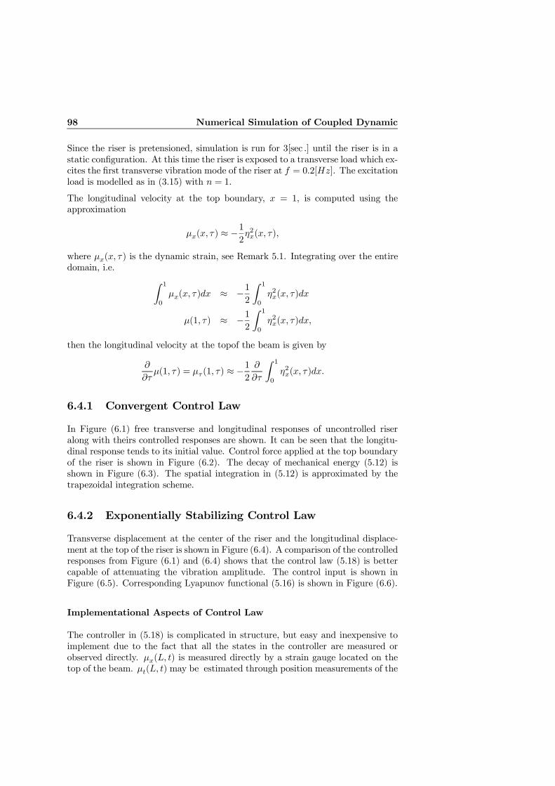
98 Numerical Simulation of Coupled Dynamic
Since the riser is pretensioned, simulation is run for 3[sec .] until the riser is in astatic configuration. At this time the riser is exposed to a transverse load which ex-cites the first transverse vibration mode of the riser at f = 0.2[Hz]. The excitationload is modelled as in (3.15) with n = 1.
The longitudinal velocity at the top boundary, x = 1, is computed using theapproximation
µx(x, τ) ≈ −1
2η2x(x, τ),
where µx(x, τ) is the dynamic strain, see Remark 5.1. Integrating over the entiredomain, i.e. Z 1
0
µx(x, τ)dx ≈ −12
Z 1
0
η2x(x, τ)dx
µ(1, τ) ≈ −12
Z 1
0
η2x(x, τ)dx,
then the longitudinal velocity at the topof the beam is given by
∂
∂τµ(1, τ) = µτ (1, τ) ≈ −
1
2
∂
∂τ
Z 1
0
η2x(x, τ)dx.
6.4.1 Convergent Control Law
In Figure (6.1) free transverse and longitudinal responses of uncontrolled riseralong with theirs controlled responses are shown. It can be seen that the longitu-dinal response tends to its initial value. Control force applied at the top boundaryof the riser is shown in Figure (6.2). The decay of mechanical energy (5.12) isshown in Figure (6.3). The spatial integration in (5.12) is approximated by thetrapezoidal integration scheme.
6.4.2 Exponentially Stabilizing Control Law
Transverse displacement at the center of the riser and the longitudinal displace-ment at the top of the riser is shown in Figure (6.4). A comparison of the controlledresponses from Figure (6.1) and (6.4) shows that the control law (5.18) is bettercapable of attenuating the vibration amplitude. The control input is shown inFigure (6.5). Corresponding Lyapunov functional (5.16) is shown in Figure (6.6).
Implementational Aspects of Control Law
The controller in (5.18) is complicated in structure, but easy and inexpensive toimplement due to the fact that all the states in the controller are measured orobserved directly. µx(L, t) is measured directly by a strain gauge located on thetop of the beam. µt(L, t) may be estimated through position measurements of the
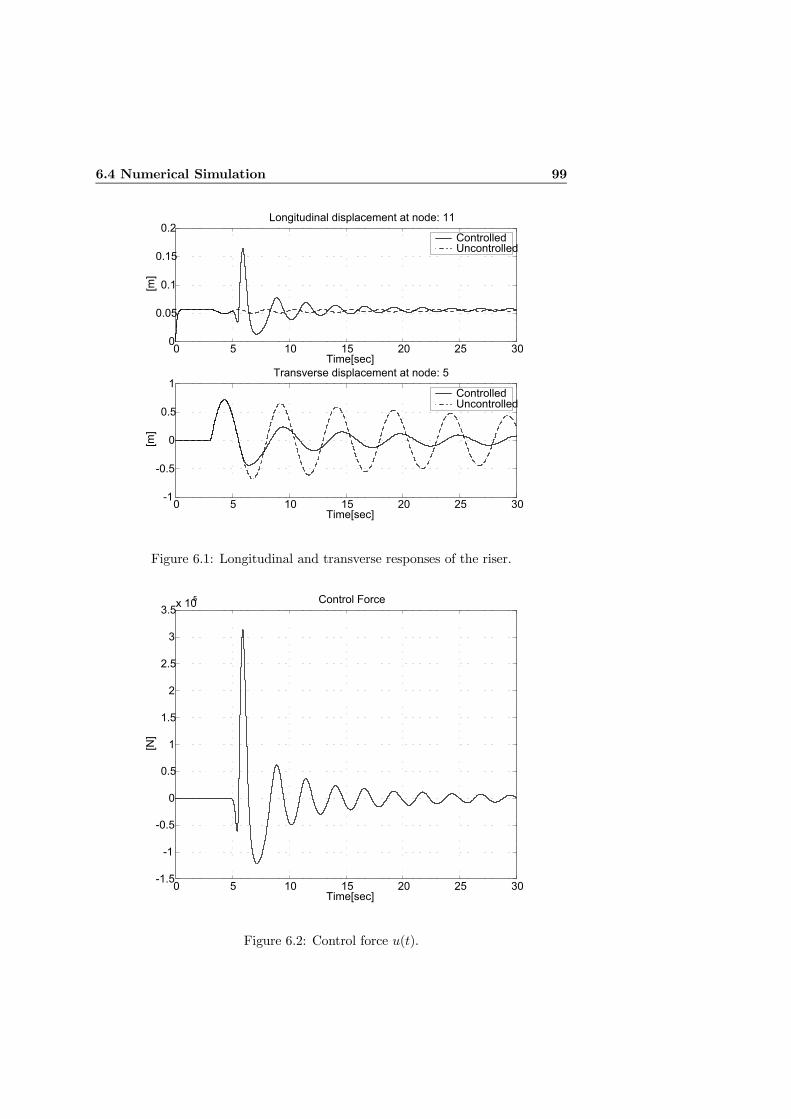
6.4 Numerical Simulation 99
0 5 10 15 20 25 300
0.05
0.1
0.15
0.2Longitudinal displacement at node: 11
[m]
Time[sec]
Controlled Uncontrolled
0 5 10 15 20 25 30-1
-0.5
0
0.5
1Transverse displacement at node: 5
[m]
Time[sec]
Controlled Uncontrolled
Figure 6.1: Longitudinal and transverse responses of the riser.
0 5 10 15 20 25 30-1.5
-1
-0.5
0
0.5
1
1.5
2
2.5
3
3.5x 10⁵ Control Force
[N]
Time[sec]
Figure 6.2: Control force u(t).
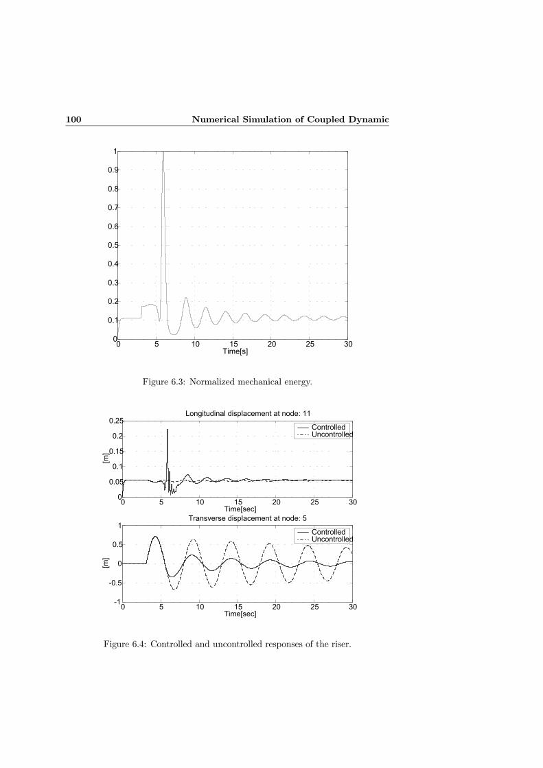
100 Numerical Simulation of Coupled Dynamic
0 5 10 15 20 25 300
0.1
0.2
0.3
0.4
0.5
0.6
0.7
0.8
0.9
1
Time[s]
Figure 6.3: Normalized mechanical energy.
0 5 10 15 20 25 300
0.05
0.1
0.15
0.2
0.25Longitudinal displacement at node: 11
[m]
Time[sec]
Controlled Uncontrolled
0 5 10 15 20 25 30-1
-0.5
0
0.5
1Transverse displacement at node: 5
[m]
Time[sec]
Controlled Uncontrolled
Figure 6.4: Controlled and uncontrolled responses of the riser.
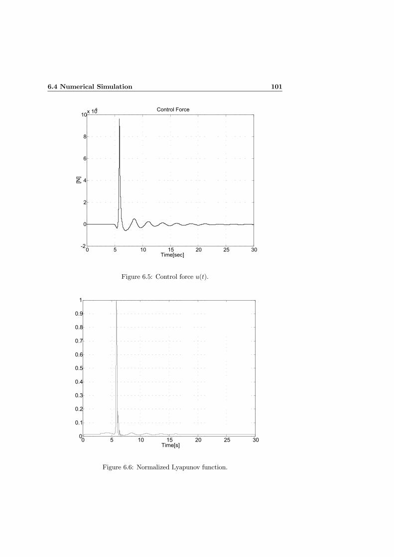
6.4 Numerical Simulation 101
0 5 10 15 20 25 30-2
0
2
4
6
8
10x 105 Control Force
[N]
Time[sec]
Figure 6.5: Control force u(t).
0 5 10 15 20 25 300
0.1
0.2
0.3
0.4
0.5
0.6
0.7
0.8
0.9
1
Time[s]
Figure 6.6: Normalized Lyapunov function.
102 Numerical Simulation of Coupled Dynamic
end position of the beam. This may be implemented in practice for marine risers bytime differentiating the stroke measures of the riser’s passive heave compensationsystem. The slope, ηx(L, t), may be directly measured by using inclinometers.
6.5 Conclusions
Performances of the proposed control laws, (5.13) and (5.18), are compared. It isclear that the control law (5.18) shows a better performance. By optimization ofcontrol gains better performance may be achieved. However, this is limited due tothe fact that compression of the riser is not allowed. Simulations also show thatthe energy of the closed-loop systems converge to their initial values.
Chapter 7
Conclusions
Nonlinearity in the strain-displacement relation has been taken into account formodelling of beams. Different nonlinear models of slender bodies based on prac-tical assumptions have been derived. In order to improve the accuracy and avoidapproximation errors the study has been based on the original models i.e. PDEs.
Passivity property of these models has been studied and based on this control lawshave been designed. A mass-damper-spring system is attached to the top bound-ary of a transversely vibrating beam, which changes the lossless passivity of thetransverse vibrating beam to output-strictly passive. Based on passivity proper-ties, simple output feedback control laws are designed to attenuate the vibrationamplitude.
A nonlinear beam model with coupling between the longitudinal and transver-sal dynamics is considered. Using Lyapunov analysis and Barbalats Lemma, twocontrol laws are derived for this system. It is proved that the energy of the ex-ponentially stabilized closed-loop system has an upper bound in the presence ofexternal disturbances.
A decoupled model of a transversely vibration beam is also studied. Two linearcontrol laws using velocity and slope feedback from the top boundary of the beamare designed. Stability of the closed-loop systems are proved. It is also provedthat in the presence of external disturbances, exponentially stabilized closed-loopsystem has an upper bounded energy and hence bounded states. Simplicity ofthe designed control laws is an attractive factor from an imlpementational pointof view. The states used by the control laws, i.e. velocity and slope at the topboundary can be directly measured or estimated through a simple state estimator.
There are reports from experimental tests of passive damping of vortex inducedvibrations in risers, see Huse (1998) and references therein. Passive devices suchas strake has been used for this purpose. However, to the best knowledge of theauthor, there are no reports on active damping of vortex induced vibrations. To beable to implement active vibration damping, active actuators must be designed.This work should be considered as a first step towards active damping of VIV.
104 Conclusions
Analysis and simulation results seems promising. However, it is important toconduct experimental tests to confirm the results from this study and also toreveal practical obstacles.
Boundary control might be applicable to very long risers, approx. 1500m. Suchrisers can be divided to subsegments and then applying boundary control to eachof these segments. However, this requires a deeper study of the problem. Forinstance, continuity and compatibility of the boundary conditions of each segmentrelative to the neighboring segment is an important issue. This is an open topicwhich will become more important due to the fact that exploration of oil and gasfrom deeper sea becomes more usual.
Bibliography
Aamo, O. M. & Fossen, T. I. (1999), ‘Controlling line tension in thruster assistedmooring systems’, Proceedings of IEEE Conference on Control Applications(CCA’99). Hawaii. pp. 22—26.
Aker Maritime, M. H. (1998), Active Heave Compensator, Technical Bulletin, Kris-tiansand, Norway.
Aker Maritime, M. H. (1999), Specification for Direct Riser Tensioner System, 4Cylinders, Technical Manual, Kristiansand, Norway.
Aker Mritime, M. H. (1999), Specification for Riser Tensioner System, TechnicalManual, Kristiansand, Norway.
Ames, W. F. (1965), Nonlinear Partial Differential Equations in Engineering, Aca-demic Press.
Baicu, C. F., Rahn, C. D. & Nibali, B. D. (1996), ‘Active boundary controlof elastic cables: Theory and experiment’, Journal of Sound ans Vibration198(1), 17—26.
Balas, M. J. (1977), ‘Active control of flexible systems’, Proceeding of the AIAASymposium on Dynamic and Control of Large Flexible Spacecraft, Blacksburg,Va. pp. 217—236.
Balogh, A. & Krstic, M. (1999), ‘Boundary control of the korteweg-de vries-burgersequation: Further results on stabilization and numerical demonstration’, Ac-cemted for IEEE Transaction on Automatic Control .
Balogh, A. & Krstic, M. (2000), ‘Burgers’ equation with nonlinear boundary feed-back: h1 stability, well-posedness and simulation’, To appear in MathematicalProblems in Engineering .
Barbâlat (1959), ‘Systémes d’Équations différentielles d’Oscillations non linéaires’,Revue de Mathématiques Pures et Appliquées 4(2), 267—270.
Burke, B, G. (1974), ‘An analysis of marine risers for deep water’, Journal ofPetroleum Technology .
Clough, R. W. & Penzien, J. (1975), Dynamics of Structures, McGraw Hill Inc.
106 BIBLIOGRAPHY
Coron, J.-M. & D’Andréa-Novel, B. (1998), ‘Stabilization of a rotating body beamwithout damping’, IEEE Transaction on Automatic Control 43(5), 608—618.
de Queiroz, M. S., Dawson, D. M., Agarwal, M. & Zhang, F. (1999), ‘Adaptivenonlinear boundary control of a flexible link robot arm’, IEEE Transactionson Robotics and Automation 15(4), 779—787.
Desoer, C. & Vidyasagar, M. (1975), Feedback Systems: Input-Output Properties,Academic Press, New York.
Dym, C. L. (1974), Stability Theory and its Applications to Structural Mechanics,Noordhoff International Publishing, Leyden, The Netherlands.
Faltinsen, O. M. (1990), Sea Loads on Ships and Offshore Structures, CambridgeUniversity Press, U.K.
Fard, M. P. & Sagatun, S. I. (1999), ‘Exponential stabilization of a transversely vi-brating beam via boundary control’, Journal of Sound and Vibration . Sched-uled for publication in January 2001.
Fard, M. P. & Sagatun, S. I. (2000a), ‘Boundary control of a transversely vi-brating beam via lyapunov method’, Proceedings of 5th IFAC Conference onManoeuvring and Control of Marine Craft. Aalborg, Denmark. pp. 263—268.
Fard, M. P. & Sagatun, S. I. (2000b), ‘Exponential stabilization of a transverselyvibrating beam by boundary control via lyapunov’s direct method’, Journalof Dynamic Systems, Measurement, and Control . Submitted.
Fard, M. P. & Sagatun, S. I. (2000c), ‘Passivity analysis of nonlinear euler-bernoullibeams’, IEEE Transactions on Automatic Control . Submitted.
Ferrari, J. A. & Bearman, P. W. (1999), ‘Hydrodynamic loading and responseof offshore risers’, Offshore Mechanics and Arctic Engineering p. Paper No.4132.
Finn, L. (1998), ‘Reliable riser systems for spars’, 17th International Conferenceon Offshore Mechanics and Arctic Engineering p. Paper No. 602.
Fossen, T. I. (1994), Guidance and Control of Ocean Vehicles, John Wiley andSons Ltd.
Fung, R. F. & Tseng, C. C. (1999), ‘Boundary control of an axially moving stringvia lyapunov method’, Journal of Dynamic Systems, Measurement, and Con-trol 121, 105—110.
Fung, R. F., Wu, J. W. & Wu, S. L. (1999), ‘Stabilization of an axially mov-ing string by nonlinear boundary feedback’, Journal of Dynamic Systems,Measurement, and Control 121, 117—121.
Griffin, O. (1985), ‘Vortex-induced vibrations of marine cables and structures’.NRL Memorandum Report 5600, Naval Research Laboratory.
BIBLIOGRAPHY 107
Griffin, O. M. (1992), ‘Vortex-induced vibrations of marine structures in uniformand sheared flows’, pp. 293—316.
Griffin, O. M., Skop, R. A. & Koopmann, G. H. (1973), ‘The vortex-excitedresonant vibration of circular cylinders’, Journal of Sound and Vibrations31(2), 235—249.
Griffin, O. M., Skop, R. A. & Ramberg, S. E. (1975), ‘The resonant vortex vibra-tions of structures and cable systems’, pp. 731—744. Paper no. 2319.
Habib, M. S. & Radcliffe, C. J. (1991), ‘Active parametric damping of distributedparameter beam transverse vibration’, Journal of Dynamic Systems, Mea-surement, and Control 113(295), 295—299.
Huse, E. (1998), Riser wake interaction: Effect of strakes on riser interaction,Technical Report 513136.00.02, MARINTEK Report.
Khalil, H. K. (1996), Nonlinear Systems, second edn, Prentic Hall.
Krabs, W. & Leugering, G. (1994), ‘On boundary controllability of one-dimensional vibrating systems by w1,p0 -controls for p ∈ [2,∞]’, MathematicalMethods in the Applied Sciences 17, 77—93.
Krstic, M. (1999), ‘On global stabilization of burgers’ equation by boundary con-trol’, Systems & Control Letters 37, 123—142.
Larsen, C. M. (1995), Marine riser analysis, Technical Report NA550/655, De-partment of Naval Architecture and Marine Engineering, The University ofMichigan.
Larsen, C. M. & Halse, K. H. (1997), ‘Comparison of models for vortex inducedvibrations of slender marine structures’, Marine Structures 10, 413—441.
Larsen, C. M., Vandiver, J. K., Vikestad, K. & Lie, H. (n.d.), ‘Vortex inducedvibration of long marine risers, experimental investigations of multi-frequencyresponse’.
Liu, W.-J. & Krstic, M. (2000), ‘Backstepping boundary control of burgers’ equa-tion with actuator dynamics’, Systems & Control Letters 41, 291—303.
Luo, Z. H. (1993), ‘Direct strain feedback control of flexible robot arms: New the-oretical and experimental results’, IEEE Transaction on Automatic Control38(11), 1610—1622.
Luo, Z. H., Nobuyuki, K. & Guo, B. Z. (1995), ‘Shear feedback control of flexiblerobot arms’, IEEE Transactions on Robotics and Automation 11(5), 760—765.
Matsuno, K. & Murata, K. (1999), ‘Passivity and PDS control of flexible me-chanical systems on the basis of distributed parameter system’, Preceedingsof IEEE International Conference on Systems, Man, and Cybernetics.Tokyo,Japan. pp. 51—56.
Meirovitch, L. (1997), Principles and Techniques of Vibrations, Prentice-Hall, Inc.
108 BIBLIOGRAPHY
Meirovitch, L. & Baruk, H. (1983), ‘On the problem of observation spillover inself-adjoint distributed-parameter systems’, Journal of Optimization and Ap-plications 30(2), 269—291.
Mitchell, A. R. & Griffiths, D. F. (1980), The Finite Difference Method in PartialDifferential Equations, John Wiley and Sons, U.K.
Morgan, G. W. & Peret, J. W. (n.d.), ‘Applied mechanics of marine riser systems’,Petroleum Engineer, Series of articles, Oct. 1971-Jan. 1976 .
Nayfeh, A. & Mook, D. (1979), Nonlinear Oscillations, Wiley-Interscience, NewYork.
Ottosen, N. & Petersson, H. (1992), Introduction to the Finite Element Method,Prentice Hall, U. K.
Richtmyer, R. D. & Morton, K. W. (1967), Difference Methods for Initial-ValueProblems, second edn, John Wiley and Sons, New York.
Sarpkaya, T. & Shoaff, R. L. (1979), A discrete vortex analysis of flow aboutstationary and transversely oscillating cylinders, Technical Report Tech. Rep.NPS-69 SL 79011, Nav. Postgrad. Sch., Monterey, California.
Sevin, E. (1960), ‘On the elastic bending of columns due to dynamic axial forcesincluding effects of axial inertia’, Journal of Applied Mechanics pp. 125—131.
Shahruz, S. M. (1997), ‘Suppression of vibration in stretched strings by the bound-ary control’, Proceedings of the 36th Conference on Decesion and Control ,San Diego, California USA pp. 535—536.
Shahruz, S. M. & Krishna, L. G. (1996), ‘Boundary control of a non-linear string’,Journal of Sound and Vibration 195(1), 169—174.
Shahruz, S. M. & Narasimha, C. A. (1997), ‘Suppression of vibration instretched strings by the boundary control’, Journal of Sound and Vibration204(5), 835—840.
Shames, I. H. & Dym, C. L. (1985), Energy and Finite Element Methods in Struc-tural Mechanics, Taylor and Francis, U.S.A.
Smith, G. D. (1978), Numerical Solution of Partial Differential Equations: FiniteDifference Methods, second edn, Clarendon Press, Oxford.
Spong, M. W. & Vidyasagar, M. (1989), Robot Dynamics And Control, John Wileyand Sons.
Strouhal, V. (1878), ‘Uber eine besondere art der tonerregung’, Annalen der Physikand Chemie Band V pp. 216—251.
Triantafyllou, M. S. (1990), Cable mechanics with marine applications, Techni-cal report, Department of Ocean Engineering, Massachusettes Institute ofTechnology.
BIBLIOGRAPHY 109
Van der Schaft, A. J. (1996), L2-Gain and Passivity Techniques in Nonlinear Con-trol, Vol. 218 of Lecture Notes in Control and Information Sciences, SpringerVerlag, Heidelberg.
Vandiver, J. K. (1993), ‘Dimensionless parameters important to the prediction ofvortex-induced vibration of long, flexible cylinders in ocean currents’, Journalof Flouids amd Structures 7, 423—455.
Vikestad, K. (1998), Multi-Frequency Response of a Cylinder Subjected VortexShedding and Support Motions, PhD thesis, Norwegian University of Scienceand Technology.
Walker, J. A. (1980), Dynamical Systems and Evolution Equations, Plenum Press,New York.
Wang, P. K. (1966), ‘Stability analysis of elastic and aeroelastic systems via lya-punov’s direct method’, Journal of the Franklin Institute 281(1), 51—72.
Willems, J. (1972), ‘Dissipative dynamical systems, part I and II’, Archieve forRational Mechanics and Analysis 45, 321—393.
Woodall, S. R. (1966), ‘On the large amplitude oscillations of a thin elastic beam’,International Journal of Nonlinear Mechanics 1, 217—238.
Zubov, V. L. (1964), Methods of A. M. Lyapunov and Their Application, Noord-hoff, Ltd, Gorning, Netherland.

110 BIBLIOGRAPHY
Appendix A
Mathematical Preliminaries
Lyapunov’s stability theorems for lumped-parameter, discrete, systems are wellestablished and known in the control community. However, concepts and theoriesdeveloped for such systems cannot be directly carried over to distributed parame-ter systems. We intend to introduce stability theorems for distributed-parametersystems which deem to be relevant to the analysis in this work.
A.1 Passivity
A brief introduction to passivity is given here. The reader is referred to Van derSchaft (1996), Desoer & Vidyasagar (1975) and Willems (1972) for a comprehen-sive treatment of the topic.
Assume that total energy of a mechanical system, sum of kinetic and potential,at time t is given by V (t). Let the mechanical energy stored in the system atthe initial time t = 0 be denoted by V (0) ≥ 0. Since the energy V (T ) must bepositive and lower bounded, the total system is defined as passive if and only ifthe mechanical energy dissipated by the system is less than or equal to the initialenergy stored in the system, V (0). This can be expressed as
V (T ) ≤ V (0) +Z T
0
y(t)u(t)dt (A.1)
where y(t) and u(t) are input and output of the system respectively. Notice thatthe integral in (A.1) represents the external energy input. This definition can alsobe formulated in terms of rate of change of energy and instantaneous power flowas
V (t) ≤ y(t)u(t) ∀t.
This is, the power flow into the system must be greater than or equal to the rateof change of the energy stored in the system.
112 Mathematical Preliminaries
Definition A.1 A system with input u(t) and measurement y(t) is said to bepassive if there exists a continuously differentiable positive semidefinite function
V (t), called storage function, such that
uT (t)y(t) ≥ V (t) + ²uT (t)u(t) + δyT (t)y(t) (A.2)
where ², δ are nonnegative constants. The system is said to be
• lossless if (A.2) is satisfied with equality and ² = δ = 0, that is
uT (t)y(t) = V (t)
• input strictly passive if ² > 0,• output strictly passive if δ > 0,• input and output strictly passive if ² > 0 and δ > 0.
A.2 Definitions and Theorems for Lyapunov Func-tionals
The main theorems are restated from references, Zubov (1964), Wang (1966), Dym(1974) and Khalil (1996). Consider a set of 2n partial differential equations of theform
∂vi∂t
= fi
Ãt, xj , vm,
∂vm∂xj
, · · · , ∂v(γi)m
∂x(γi)j
!, i = 1, ..., 2n, m = 1, ..., 2n and j = 1, ..., k
(A.3)
where xj denotes spatial coordinate and t is the time variable. The highest orderof derivatives appearing in each equation is denoted by γi. The variables v1, ..., vnare usually associated with displacement components, while vn+1, ..., v2n will beassociated with velocity components. Equation (A.3) is defined in a certain re-gion D of the K−dimensional Euclidean space Ek. In addition to (A.3), a setof appropriate boundary conditions and smoothness conditions will be specified.The smoothness conditions refer to differentiability and continuity conditions forv1, ..., v2n in D.
Consider the functional space H2pB , whereH2pB is the Sobolev space consisting of allfunctions for which the (weak) partial derivatives up to order 2p belong to Hilbertspace L2. H2pB is the subset of H2p consisting of all functions which also satisfythe boundary conditions. We assume that ν(x, t) is sufficiently smooth, such thatwe can ignore the difference between the weak and the ordinary derivatives. Thefunctional space H2pB is composed of real vector elements
φ =£φ1 · · · φ2n
¤T.
A.2 Definitions and Theorems for Lyapunov Functionals 113
Let
ν =£v1 · · · v2n
¤Twhere the components vi are then dependent variables of (A.3). We assume thatfor any element ν(t0) ∈ H2pB , initial state, there exists a unique solution ν(t) =ν(t,ν(t0)) of the boundary value problem having the following properties:
i) ν(t,ν(t0)) is defined ∀ t ≥ t0.ii) ν(t,ν(t0)) is continuous in both its arguments.
iii) ν(t,ν(t0)) = ν(t0) when t = t0.
iv) if ν(t0) = 0, then ν(t,0) = 0, ∀ t ≥ t0.
Since ν(t,ν(t0)) is a solution of the boundary value problem,
v) ν(t,ν(t0)) ∈ H2pB ,∀ t ≥ t0
and the components νi(t,ν(t0)) satisfy (A.3). Property (iv) states that the bound-ary value problem has a trivial solution, ν(t,0) = 0, which is an invariant set ofthe system. This allows us to express the stability discussion of the system interms of the stability of ν = 0.
Definition A.2 A metric space is a pair (X ,d), X a set and d a metric. Amapping d : X ×X −→ R is a metric on X provided that it possesses the
following properties:
1. d(x, y) = 0 if and only if x = y
2. d(x, y) = d(x, y) ≥ 03. d(x, y) + d(y, z) ≥ d(x, z) ∀ x, y, z ∈ X
We define a function ρ : H2pB ×H2pB −→ R such that for any two elements φ ∈ H2pBand ψ ∈ H2pB the function ρ has the mentioned properties in previous definition.
Definition A.3 An invariant set ν = 0 is called stable, with respect to ρ, iffor any ² > 0 one can find a δ > 0 such that ρ (ν(t0),0) < δ implies thatρ (ν(t,ν(t0)),0) < ε for all t ≥ 0. if in addition
ρ (ν(t,ν(t0)),0) −→ 0 as t −→ +∞then ν = 0 is called asymptotically stable with respect to ρ.
We are now ready to quote the main theorem
114 Mathematical Preliminaries
Theorem A.1 Zubov (1964) In order for the solution ν = 0 of the boundary-value problem to be stable with respect to ρ, it is necessary and sufficient that in asufficiently small neighborhood
Sr =nν ∈ H2pB | 0 ≤ ρ (ν(t,ν(t0)),0) < r
oof ν = 0 there exists a functional V having the following properties when ν ∈ Sr:
1. V is positive definite with respect to ρ, moreover V (ν(t,ν(t0))) −→ 0 uni-formly with respect to t as ρ (ν(t,ν(t0)),0) −→ 0.
2. V admits an infinitely small upper bound with respect to ρ.
3. V (ν(t,ν(t0))) is non-increasing for t ≥ t0, whenever ν(t0) ∈ Sr.If, in addition, there exist a r∗, 0 < r∗ ≤ r, such that
4. V (ν(t,ν(t0))) −→ 0 as t −→ +∞, whenever ν(t0) ∈ Sr∗, then ν = 0 isasymptotically stable with respect to ρ.
Remark 1 Positive definiteness of the Lyapunov functional V , with respect to ρ,in Theorem A.1 can be reformulated such that for any real number ε > 0 thereexist a δ > 0 such that
V (ν) > δ whenever ρ(ν,0) > ε.
Note that V is positive definite with respect to ρ if
V (ν) ≥ α ρ2(ν,0)
where α is a positive constant.
Remark 2 The second property of Lyapunov functional V indicates that the func-tional V is continuous with respect to ρ, i.e. for any ε > 0, there exists a δ > 0such that
|V (ν)| ≤ ε whenever ρ(ν,0) < δ.
Note that V admits an infinitely small upper bound with respect to ρ if
V (ν) ≤ γρ2(ν,0)
where γ is a positive constant. The reason for this property is to allow continuityof the solution of the partial differential equation with respect to the initial data.
The next theorem is restated from Walker (1980) and summarize Lyapunov’s Di-rect Method for investigating stability of an equilibrium, xe, of a dynamic sys-tem on a metric space X . Here, Fr denotes the set of all monotone functionsf : ([0, r) ⊂ R) −→ R with f(0) = 0, f(η) > 0 for all η ∈ (0, r). The existence ofat least one equilibrium xe is assumed.
A.2 Definitions and Theorems for Lyapunov Functionals 115
Theorem A.2 Walker (1980) If V : X −→ R is a continuous Lyapunov functionon the open ball Gr(xe), some r > 0, such that
V (x) ≤ V (xe) + f(d (x,xe)) ∀x ∈Gr(xe),
some f ∈Fr, then the equilibrium xe is stable. If, in addition, V (x) ≤ −g(d (x,xe))
for all x ∈Gr(x), some g ∈Fr, then xe is asymptotically stable. If in addition, there
exist real numbers c2 ≥ c1 > 0, µ > 0, k > 0, such that
V (x) ≤ −µ (V (x)− V (xe))c1 (d (x,xe))
k ≤ V (x)− V (xe) ≤ c2 (d (x,xe))k
for all x ∈Gr(xe), then xe is exponentially stable with exponent −µtk .

116 Mathematical Preliminaries
Appendix B
Proof of Lemmas
In this appendix we state the proof of some of lemmas in the thesis.
B.1 Proof of Lemma 4.1
Proof: Using the following integration by partsZ L
0
ηxxxxηtdx = ηxxxηt|L0 −Z L
0
ηxxxηtxdx
Z L
0
ηxxxηtxdx = ηxxηtx|L0 −Z L
0
ηxxηtxxdx
the equation (4.5) can be written
−EIZ L
0
[ηxxxxηt − ηxxηxxt] dx
= −EI ηxxxηt|L0 +EIZ L
0
ηxxxηtxdx+EI
Z L
0
ηxxηxxtdx
= −EIhηxxxηt|L0 − ηxxηtx|L0
i−EI
Z L
0
ηxxηtxxdx+EI
Z L
0
ηxxηxxtdx
= −EIhηxxxηt|L0 − ηxxηtx|L0
iThe identity (4.6) is obtained as follows
1
2EA
Z L
0
£η3xηxt + 3η
2xηxxηt
¤dx
=1
2EA
Z L
0
¡η3xηt
¢xdx =
1
2EA η3xηt
¯L0
118 Proof of Lemmas
The identity (4.7) is obtained as follows
P0
Z L
0
[ηxxηt + βηxηxt] dx = P0
Z L
0
[ηxxηt + ηxηxt] dx
= P0 ηxηt|L0
The identity (4.8) is rewritten using the following relationsZ L
0
xηxxxxηxdx = xηxxxηx|L0 −Z L
0
ηxxxηxdx−Z L
0
xηxxxηxxdxZ L
0
ηxxxηxdx = ηxxηx|L0 −Z L
0
η2xxdxZ L
0
xηxxxηxxdx =1
2xη2xx
¯L0− 12
Z L
0
η2xxdx
as
− γEI
Z L
0
xηxxxxηxdx
= −γEI xηxxxηx|L0 + γEI ηxxηx|L0+ γ
EI
2xη2xx
¯L0− γ
3
2EI
Z L
0
η2xxdx
= −EIγLµηxxx(L, t)ηx(L, t)−
1
2η2xx(L, t)
¶+ γEI ηxxηx|L0 − γ
3
2EI
Z L
0
η2xxdx
The identity (4.9) is obtained as follows
γP0
Z L
0
xηxxηxdx = γP0
"1
2
Z L
0
¡xη2x
¢xdx− 1
2
Z L
0
η2xdx
#
= γP0
"L
2η2x(L, t)−
1
2
Z L
0
η2xdx
#
The identity (4.10) is obtained as follows
γ3
2EA
Z L
0
xη3xηxxdx = γ3
2EA
Ã1
4
Z L
0
¡xη4x
¢xdx− 1
4
Z L
0
η4xdx
!
= γ3
2EA
Ã1
4xη4x
¯L0− 14
Z L
0
η4xdx
!
= γ3
2EA
ÃL
4η4x(L, t)−
1
4
Z L
0
η4xdx
!
B.2 Proof of Lemma 5.1 119
The identity (4.11) is obtained as follows
γρA
Z L
0
xηtηtxdx = γρA
"1
2
Z L
0
¡xη2t
¢xdx− 1
2
Z L
0
η2tdx
#
= γρA
"L
2η2t (L, t)−
1
2
Z L
0
η2tdx
#.¥
B.2 Proof of Lemma 5.1
Proof: The identity (5.8) is abtained as
EA
Z L
0
(µxµxt + µxxµt) dx = EA
Z L
0
(µxµt)x dx
= EA µxµt|L0 .
The identity (5.9) is obtained as follows
γρA
Z L
0
xµtµtxdx = γρA
"1
2
Z L
0
¡xµ2t
¢xdx− 1
2
Z L
0
µ2tdx
#
= γρA
"L
2µ2t (L, t)−
1
2
Z L
0
µ2tdx
#.
The identity (5.10) is obtained as follows
γEA
Z L
0
xµxxµxdx = γEA
"1
2
Z L
0
¡xµ2x
¢xdx− 1
2
Z L
0
µ2xdx
#
= γEA
"L
2µ2x(L, t)−
1
2
Z L
0
µ2xdx
#
Using the following relations
γ
Ã2EA
Z L
0
xηxηxxµxdx+EA
Z L
0
xη2xµxxdx
!
= γ
ÃEALη2x (L, t)µx (L, t)−EA
Z L
0
η2xµxdx
!
EA
Z L
0
ηxxµxηtdx+EA
Z L
0
ηxµxxηtdx
= EA ηxµxηt|L0 −EAZ L
0
ηxµxηtxdx
120 Proof of Lemmas
the identity (5.11) can be written as
EA
Z L
0
ηxxµxηtdx+EA
Z L
0
ηxµxxηtdx+EA
Z L
0
ηxηxxµtdx+ γEA
Z L
0
xη2xµxxdx
+EA
Z L
0
ηxηxtµxdx+EA
2
Z L
0
η2xµxtdx+ 2γEA
Z L
0
xηxxµxηxdx
= EA ηxµxηt|L0 −EAZ L
0
ηxµxηtxdx+EA
Z L
0
ηxηxxµtdx+EA
Z L
0
ηxηxtµxdx
+EA
2
Z L
0
η2xµxtdx+ γEALη2x (L, t)µx (L, t)− γEA
Z L
0
η2xµxdx
= EA ηxµxηt|L0 + γEALη2x (L, t)µx (L, t) +EA
Z L
0
ηxηxxµtdx
+EA
2
Z L
0
η2xµxtdx− γEA
Z L
0
η2xµxdx
= EA ηxµxηt|L0 + γEALη2x (L, t)µx (L, t) +EA1
2η2xµt
¯L0
− γEA
Z L
0
η2xµxdx.
Last equation is obtained using the following relation
∂
∂x
µ1
2η2xµt
¶= ηxηxxµt +
1
2η2xµxt
EA
Z L
0
ηxηxxµtdx+EA
2
Z L
0
η2xµxtdx = EA1
2η2xµt
¯L0
.