modelling and experimental model validation for a pusher ... · pdf filekeywords : pusher-type...
TRANSCRIPT
This document contains a post-print version of the paper
Modelling and Experimental Model Validation for a Pusher-typeReheating Furnace
authored by D. Wild, T. Meurer, and A. Kugi
and published in Mathematical and Computer Modelling of Dynamical Systems.
The content of this post-print version is identical to the published paper but without the publisher’s final layout orcopy editing. Please, scroll down for the article.
Cite this article as:D. Wild, T. Meurer, and A. Kugi, “Modelling and experimental model validation for a pusher-type reheating furnace”,Mathematical and Computer Modelling of Dynamical Systems, vol. 15, no. 3, pp. 209–232, 2009. doi: 10.1080/13873950902927683
BibTex entry:@article{Wild09,author = {Wild, D. and Meurer, T. and Kugi, A.},title = {Modelling and Experimental Model Validation for a Pusher-type Reheating Furnace},journal = {Mathematical and Computer Modelling of Dynamical Systems},year = {2009},volume = {15},number = {3},pages = {209--232},doi = {10.1080/13873950902927683},url = {http://www.tandfonline.com/doi/abs/10.1080/13873950902927683}
}
Link to original paper:http://dx.doi.org/10.1080/13873950902927683http://www.tandfonline.com/doi/abs/10.1080/13873950902927683
Read more ACIN papers or get this document:http://www.acin.tuwien.ac.at/literature
Contact:Automation and Control Institute (ACIN) Internet: www.acin.tuwien.ac.atVienna University of Technology E-mail: [email protected] 27-29/E376 Phone: +43 1 58801 376011040 Vienna, Austria Fax: +43 1 58801 37699
Copyright notice:This is an authors’ accepted manuscript of the article D. Wild, T. Meurer, and A. Kugi, “Modelling and experimental model validationfor a pusher-type reheating furnace”, Mathematical and Computer Modelling of Dynamical Systems, vol. 15, no. 3, pp. 209–232, 2009. doi:10.1080/13873950902927683 published in Mathematical and Computer Modelling of Dynamical Systems, copyright c© Taylor & FrancisGroup, LLC, available online at: http://dx.doi.org/10.1080/13873950902927683
March 1, 2009 12:31 Mathematical and Computer Modelling of Dynamical Systems mcmds˙wild˙08
Mathematical and Computer Modelling of Dynamical SystemsVol. 00, No. 00, July 2004, 1–20
Modelling and Experimental Model Validation for a Pusher-type Reheating Furnace
D. Wild, T. Meurer, A. Kugi
Automation and Control Institute,
Complex Dynamical Systems Group,
Vienna University of Technology, Vienna, Austria,
{wild, meurer, kugi}@acin.tuwien.ac.at
The slab reheating process turns out to play a key role in order to deal with the steadily increasing demands on the quality of hotrolled steel plates. Improvements both in the throughput of the furnace as well as the accurate realization of reheating paths for theslabs require to incorporate modern model-based control design techniques into the furnace automation. For this, suitable mathematicalmodels with manageable dimension and complexity have to be determined for the furnace and slab dynamics. In this contribution, firstprinciples are applied for the derivation of a physics-based model of the reheating process in a so-called pusher-type reheating furnace.Thereby, a discontinuous mode of furnace operation is considered, which is characterized by a varying number of slabs with variablegeometry being discontinuously moved through the furnace. This in particular results in a hybrid structure of the mathematical model.The accuracy of the mathematical model is validated by a comparison with experimental data obtained from a measurement campaignwith a test slab performed at an industrial pusher-type reheating furnace.
Keywords: Pusher-type furnace, slab reheating process, physics-based modelling, combustion modelling, singular perturbation,experimental validation
1. Introduction
Reheating of slabs from the ambient temperature to their rolling temperature of approximately 1150◦C isan important step in the heavy plate production in order to prepare the slabs for the subsequent rollingprocess. For this, the slabs are normally heated in gas- or oil-fired pusher-type reheating furnaces.In order to illustrate this, a schematic setup of the furnace, which is considered in the following, is shown
in Figure 1. Depending on the location of the burners, the local temperature range, and the dwell of theslabs, the furnace can be structurally divided into the convective zone without burners, the pre-heatingzone, the heating zone as well as the pre-soaking and the soaking zone. In the convective zone an initialheating of the cold slabs entering the furnace occurs due to the heat radiation and the convective flowof hot exhaust gas which is directed towards the funnel. In the two heating zones the slabs are heatedup to their pre-planned rolling temperature in order to achieve the desired metallurgical transitions. Thehomogenisation of the slabs by diffusive processes inside the material finally occurs in the two soaking zones.Note that every zone except the convective zone is equipped with burners whose fuel and combustion airflows can be adjusted autonomously for each zone.In the typical operation mode cold slabs are pushed into the furnace in up to three parallel rows at
the position z = 0 while the readily heated slabs are pulled out of the furnace on the opposite side atz = Lz. Note that new slabs can only enter the furnace whenever heated slabs are pulled out of the furnace.The majority of pusher-type furnaces is continuously fed with slabs of the same geometry such that thefurnace is operated in a quasi-steady state with rather constant working conditions. However, dependingon the integration of the pusher-type furnace within the overall production process, configurations arisewhere the furnace is fed discontinuously with slabs of varying geometry and differing desired heating andhomogenisation paths. Due to the coupling of the time-continuous heat exchange and flow processes withthe discrete switching of the slab movement along the z-direction, the thus operated pusher-type furnace
Gusshausstrasse 27-29 / E376, A-1040 Vienna, Austria, Phone: +43 (0)1 58801-77628, Fax: +43 (0)1 58801-37699
Mathematical and Computer Modelling of Dynamical SystemsISSN: 1387-3954 print/ISSN 1744-5051 online c© 2004 Taylor & Francis
http://www.tandf.co.uk/journalsDOI: 10.1080/13873950xxxxxxxxxxxxx
Post-print version of the article: D. Wild, T. Meurer, and A. Kugi, “Modelling and experimental model validation for a pusher-type reheatingfurnace”, Mathematical and Computer Modelling of Dynamical Systems, vol. 15, no. 3, pp. 209–232, 2009. doi: 10.1080/13873950902927683The content of this post-print version is identical to the published paper but without the publisher’s final layout or copy editing.

March 1, 2009 12:31 Mathematical and Computer Modelling of Dynamical Systems mcmds˙wild˙08
2 D. Wild, T. Meurer, and A. Kugi
z = 0z = Lz
x
y
funnel
burners valve
slab movement
slab
soaking pre-soaking heating pre-heating convectivezonezonezonezonezone
Figure 1. Schematic illustration of a typical pusher-type reheating furnace heated with gas and/or oil burners.
can be classified as a hybrid system.This operation mode in particular requires to include state-of-the-art automation facilities in order to
cope with the steadily increasing demands on product quality and the increasing production rates in hotrolling mills. For this, both advanced optimization strategies to determine the suitable entering sequenceof the slabs in view of their individual heating and homogenisation paths and modern model-based controltechniques to realize the heating strategy have to be incorporated. Thereby, the major difficulty is thefact that it is desired to control the individual slab temperatures without the possibility to measure theslab temperatures inside the furnace. Hence, an appropriate mathematical model has to be derived inorder to numerically reconstruct the slab temperatures during the reheating process. Thereby, on the onehand the highly complex furnace dynamics including the combustion of fuel, the gas mass flows withinthe non-trivial geometry of the furnace and the energy exchange between the slabs, the gas and the wallshas to be captured by a suitable mathematical model. On the other hand, a manageable complexity of themathematical model has to be retained in view of control design and its real-time implementation.For computational modelling, system analysis, and simulation, the application of methods originating
from computational fluid dynamics (CFD) often allows to obtain an accurate spatial and temporal res-olution of the mass flow and heat transfer mechanisms inside the furnace. However, these advantages ofCFD–based approaches are overwhelmed by the large number of system variables reaching up to severalmillion quantities depending on the level of detail. Hence these tools are commonly used for designingnew furnaces and to perform off-line studies of the gas and/or combustion dynamics [1,2]. A reduction ofthe calculating time compared to conventional CFD techniques is achieved by combining the CFD simula-tion with the classical zone method [3]. Although providing promising results in view of resolving the gasdynamics and the heat transfer mechanisms, this approach still lacks to provide analytical mathematicalmodels of medium complexity and dimension, which are the basis for model-based control design.On the other hand, in many industrial applications a pragmatic modelling approach is considered, which
traces back to [4]. Therein, a sufficiently large number of local furnace temperature measurements obtainedfrom suitably distributed thermocouples serve as inputs for a slab-heating model, see, e.g., [5,6]. This allowsto evaluate the respective slab temperature profiles in real-time. In view of control design as well as processoptimization the main drawback of this approach arises from the missing relation between the measuredfurnace temperatures and their realization by the physical inputs, namely fuel and combustion air.As a promising alternative avoiding the high number of system variables while preserving the physical
relation between the system state and input quantities, the so-called zone method as proposed in [7], isextensively studied in [8, 9]. Thereby, the furnace is subdivided into gas volumes, wall and slab elementswhose radiative heat exchange is calculated utilizing coupling factors. Furthermore, this approach assumesa continuous furnace operation mode and steady state conditions for the wall and gas temperature. The
Post-print version of the article: D. Wild, T. Meurer, and A. Kugi, “Modelling and experimental model validation for a pusher-type reheatingfurnace”, Mathematical and Computer Modelling of Dynamical Systems, vol. 15, no. 3, pp. 209–232, 2009. doi: 10.1080/13873950902927683The content of this post-print version is identical to the published paper but without the publisher’s final layout or copy editing.
March 1, 2009 12:31 Mathematical and Computer Modelling of Dynamical Systems mcmds˙wild˙08
Modelling and Experimental Model Validation for a Pusher-type Reheating Furnace 3
available results on furnace modelling utilizing the zone method are based on the assumption of a contin-uous furnace operation, i.e. uniform slab geometries, target temperatures, and slab movements. However,this is no longer satisfied in the furnace under consideration.Therefore, in the following a physics-based modelling approach is considered for the discontinuous op-
eration mode of the reheating furnace depicted in Figure 1. For this, according to the zone method, inSection 2 the furnace is discretized along the z-direction into control volumes. In each control volume, massand energy balances are applied for modelling the dynamics of the exhaust gas composition as well as therespective gas temperature. In addition, the temperature evolution in the surrounding wall elements andthe slabs is incorporated in the system description. Since thermal radiation represents the major modeof energy exchange inside the furnace, the so–called net-radiation method is used in Section 3 to deter-mine the heat flows coupling the individual sub-models of the gas composition, the gas temperature, thewall temperature, and the slab temperature inside the furnace. This is followed by the assembling of thesub-models into a single model describing the overall reheating process in the furnace. Furthermore, abrief discussion on the computational implementation of this model is given in Section 4. The accuracyof the determined model is validated in Section 5 by comparing numerical results and measurement dataobtained from a measurement campaign at the AG der Dillinger Huttenwerke, Dillingen (Germany). Somefinal remarks conclude the paper.
Nomenclature of some important quantities
Aisj area of the j-th slab surface inside the i-th control volume
Asj surface area of the j-th slabAwi
surface area of the i-th wall elementQgi,sj heat flow between the i-th gas space and the j-th slab surface
Qgi,wkheat flow between the i-th gas space and the k-th wall surface
Qwi,sj heat flow between the i-th wall and the j-th slab surfacegi index denoting the i-th control volume, i = 1, . . . , 2Nv
magi
combustion air mass flow into the i-th control volume
mfgi fuel mass flow into the i-th control volume
mingi
mass flow into the i-th control volume, i.e. out of the (i+ 1)-th into the i-th control volume
moutgi
mass flow out of the i-th control volume, i.e. out of the i-th into the (i− 1)-th control volumeNslab number of slabs charged into the furnaceNv number of discretized control volumes of a furnace sectionsj index denoting the j-th slab, j = 1, . . . , Nslab
T g vector of the gas temperatures Tgifor i = 1, . . . , 2Nv
T s vector combining all slab temperature vectors T sj of all slabs for j = 1, . . . , Nslab
Tw vector of the wall surface temperatures Twifor i = 1, . . . , 2Nv
ug vector combining all input vectors ugiof all control volumes for i = 1, . . . , 2Nv
wg vector combining all vectors wgiof all control volumes for i = 1, . . . , 2Nv
Tgigas temperature in the i-th control volume
Tsj temperature distribution along the height of the j-th slab, i.e. Tsj(t, y)T sj vector of the spatially discretized temperatures Tsj of the j-th slabTwi
wall surface temperature of the i-th wall elementugi
input vector of the i-th control volumewgi
vector of mass fractions of all species inside the i-th control volumewi index denoting the wall surrounding the i-th control volume, i = 1, . . . , 2Nv
wνgi
mass fraction of the ν-th species in the i-th control volume
Post-print version of the article: D. Wild, T. Meurer, and A. Kugi, “Modelling and experimental model validation for a pusher-type reheatingfurnace”, Mathematical and Computer Modelling of Dynamical Systems, vol. 15, no. 3, pp. 209–232, 2009. doi: 10.1080/13873950902927683The content of this post-print version is identical to the published paper but without the publisher’s final layout or copy editing.

March 1, 2009 12:31 Mathematical and Computer Modelling of Dynamical Systems mcmds˙wild˙08
4 D. Wild, T. Meurer, and A. Kugi
volume 1volume Nv
volume 2Nv volume Nv + 1
. . .
. . .
. . .
. . .
upper section
lower section
Figure 2. Schematic illustration of the furnace discretization into control volumes for the upper (volumes 1 to Nv) and the lowerfurnace section (volumes Nv + 1 to 2Nv).
2. Mathematical modelling
In this section, a physics-based mathematical model is presented for the pusher-type reheating furnaceshown in Figure 1. It is thereby desired that the derived model accurately reflects the fundamental dynamicsof the reheating process. Secondary and from a modelling and validation point of view only hardly accessibleeffects such as the detailed fluid flow within the furnace or the influence of the flame geometry are neglectedin order to retain a model of manageable dimension and complexity.For modelling purposes, the furnace is split up into an upper and a lower section as shown in Figure
2. According to the zone method [7, 10], each section is divided into Nv control volumes with respect tothe z-direction in order to accurately approximate the furnace shape and to ensure that (almost) everycontrol volume contains a thermocouple. Note that the latter requirement is in particular important forthe subsequent experimental validation.Furthermore, it is assumed that temperature deviations occur only along the z-coordinate, i.e. over the
length of the furnace. This simplification is motivated by the fact that all burners within a furnace zone areactuated by a common valve for fuel and combustion air, such that it is not directly possible to influencethe temperature distribution along the width and height of the upper and lower furnace section. In thefollowing, the governing equations for the exhaust gas composition as well as the gas temperature, the walltemperature, and the slab temperature distribution are exemplarily derived for the i-th control volumeand the j-th slab by applying first principles. The overall system model can then be easily assembled fromthese subsystems.
2.1. Gas and combustion dynamics
For the modelling of the exhaust gas dynamics, at first the components G of the furnace atmosphere areidentified and divided into the sets Go, Ga, and Ge denoting the oxidizable components, the combustionair components, and the combustion products, i.e. the exhaust gas generated from the combustion of Go
with Ga, respectively. In particular, the oxidizable components can be identified as hydrogen (H2), carbonmonoxide (CO), and hydrocarbon gases like methane (CH4), ethane (C2H6), etc., such that Go is givenin the form Go = {H2,CO,CH4,C2H6, . . . }. The combustion air is assumed to be a mixture of nitrogen(N2) and oxygen (O2), i.e. Ga = {N2,O2}. Hence, the resulting group of exhaust gases consists mainlyof the combustion products vapor (H2O) and carbon dioxide (CO2), i.e. Ge = {H2O,CO2}. In order toincrease the level of detail also incomplete combustion and dissociation products can be included in Ge.In the following, the composition of the mass mgi
of gas stored in the i-th control volume is expressed interms of mass fractions wν
gisuch that the mass of an individual component ν ∈ G = Go ∪Ga ∪Ge inside
the volume is given by mνgi
= mgiwνgi
while∑
ν∈Gwνgi
= 1.As illustrated in Figure 1, the mass flow in each control volume is dominated by the flow directed
towards the funnel, i.e. in the sequel it is assumed that all mass flows are oriented in negative z-direction.
Post-print version of the article: D. Wild, T. Meurer, and A. Kugi, “Modelling and experimental model validation for a pusher-type reheatingfurnace”, Mathematical and Computer Modelling of Dynamical Systems, vol. 15, no. 3, pp. 209–232, 2009. doi: 10.1080/13873950902927683The content of this post-print version is identical to the published paper but without the publisher’s final layout or copy editing.

March 1, 2009 12:31 Mathematical and Computer Modelling of Dynamical Systems mcmds˙wild˙08
Modelling and Experimental Model Validation for a Pusher-type Reheating Furnace 5
mingi mout
gi
mfgi , m
agi
Tgi,mgi
, Vgi, p
x
y
z
Qgi
volume ivolume i+ 1 volume i− 1
slab j slab j − 1
Figure 3. Schematic diagram of the i-th control volume.
Furthermore, we assume an isobaric furnace process at constant pressure p, which is ensured in the realplant by an appropriately controlled valve inside the funnel. Considering the i-th control volume as shown inFigure 3, the mass flows entering and leaving the control volume are denoted as min
giand mout
gi, respectively.
The quantities mfgi and ma
gidescribe the fuel and air mass flow into the volume due to the attached
burners. The respective compositions are similarly expressed by the mass fractions win,νgi , wout,ν
gi , wf,νgi ,
and wa,νgi . In order to simplify the notation, in the subsequent mass balances the sum of the fuel and
air mass flows are abbreviated by mbgi
= mfgi + ma
giwhile the respective mass fraction follows as wb,ν
gi =
(mfgiw
f,νgi + ma
giwa,νgi )/mb
gi. According to Figure 3 mass conservation of the stored mass mgi
inside thecontrol volume Vgi
yields
dmgi
dt= min
gi+ mb
gi− mout
gi(1)
while mass balancing for the respective components ν ∈ G results in
dmνgi
dt= min
giwin,νgi
+ mbgiwb,νgi
− moutgi
wout,νgi
+ VgiMν rνgi
. (2)
Here, the term Mν denotes the molar weight of the component ν while rνgirepresents the mass generation
rate of the component ν resulting from the chemical reactions of the combustion process. Hence, a positivegeneration rate rνgi
> 0 indicates the production of the species ν while a negative generation rate rνgi< 0
indicates the degradation of ν [11]. Note that the generation rate rνgiin general depends on the temperature
of the reactants and their mass fractions wνgi
inside the control volume and will be discussed below.
Substitution of (1) into (2) and assuming ideal mixing conditions inside the gas volume, i.e. wout,νgi = wν
gi
for all ν ∈ G, a set of ordinary differential equations (ODEs)
mgi
dwνgi
dt= min
gi
(win,νgi
− wνgi
)+ mb
gi
(wb,νgi
− wνgi
)+ Vgi
Mν rνgi, ν ∈ G (3)
for the mass fractions is obtained in terms of the incoming mass flows, their mass fractions, and the reactionrate. Recall that the considered furnace is operated at a constant pressure p. Hence, by assuming ideal-gasbehavior, the stored mass mgi
in the i-th control volume with volume Vgican be easily determined from
the ideal gas law as a function of the gas temperature Tgiand the mass fractions wν
gi, ν ∈ G, i.e.
mgi=
pVgi
RTgi
∑ν∈G
wνgi
Mν
(4)
with R the universal gas constant [12]. Hence, for given mingi
and mbgi
differentiation of (4) with respect
Post-print version of the article: D. Wild, T. Meurer, and A. Kugi, “Modelling and experimental model validation for a pusher-type reheatingfurnace”, Mathematical and Computer Modelling of Dynamical Systems, vol. 15, no. 3, pp. 209–232, 2009. doi: 10.1080/13873950902927683The content of this post-print version is identical to the published paper but without the publisher’s final layout or copy editing.
March 1, 2009 12:31 Mathematical and Computer Modelling of Dynamical Systems mcmds˙wild˙08
6 D. Wild, T. Meurer, and A. Kugi
to time t in view of (3) allows to compute the mass flow moutgi
leaving the control volume. However, thisrequires the knowledge of the time evolution of the gas temperature Tgi
.For this, the energy balance for the control volume is set up by considering the change of the stored
enthalpy Hgi, i.e.
dHgi
dt= −Qgi
+ Hbgi+ H in
gi− Hout
gi, (5)
where Qgisummarizes the energy exchange between the gas volume and the slabs as well as the walls.
A detailed calculation of Qgiis given in Section 3. The enthalpy flow Hb
gifrom the burners consists of
the enthalpies associated with the fuel mass flow mfgi at temperature T f
gi and with the mass flow of thepre-heated air ma
giat temperature T a
gi. This yields
Hbgi= mf
gi
∑
ν∈Gf
wf,νgi
hν(T fgi) + ma
gi
∑
ν∈Ga
wa,νgi
hν(T agi), (6)
where hν(T ) denotes the absolute specific enthalpy1 of the species ν at temperature T and Gf ⊂ Gsummarizes the components of the fuel. Note that typically the furnaces used in hot rolling mills are firedwith not necessarily constant mixtures of coke oven gas, natural gas, and blast furnace gas. Hence, thefuel is a mixture of oxidizable and non-combustible components. Since Gf ⊂ G, the subsequent notation
is simplified by extending wf,νgi and wa,ν
gi to G with the choice wf,νgi = 0 and wa,ν
gi = 0 if ν ∈ G but ν 6∈ Gf
or ν 6∈ Ga, respectively.Besides the energy input from the burners, the exhaust gas min
gifrom the previous control volume enters
the considered control volume at the temperature T ingi. Equivalently, energy is transferred to the next
control volume by the mass flow moutgi
at the temperature T outgi
such that
H ingi
= mingi
∑
ν∈Gwin,νgi
hν(T ingi), Hout
gi= mout
gi
∑
ν∈Gwout,νgi
hν(T outgi
). (7)
Recall that the stored mass-specific enthalpy is given as Hgi= mgi
hgiwith the mass specific enthalpy hgi
=∑ν∈G hν(Tgi
)wνgi. Hence, by considering the total differential of the mass-specific enthalpy of the mixture
inside the control volume under isobaric conditions [11], i.e. dhgi= cp,gi
dTgi+∑
ν∈G hνdwνgi
with thespecific heat capacity for ideal mixtures of the gas components cp,gi
=∑
ν∈Gwνgicνp,gi
, cνp,gi= ∂hν/∂Tgi
|wνgi,
it follows in view of (5) with (2), (6), (7) that
mgicp,gi
dTgi
dt= −Qgi
− Vgi
∑
ν∈GMν rνgi
hν(Tgi) + min
gi
∑
ν∈Gwin,νgi
[hν(T in
gi)− hν(Tgi
)]
+ mfgi
∑
ν∈Gwf,νgi
[hν(T f
gi)− hν(Tgi
)]+ ma
gi
∑
ν∈Gwa,νgi
[hν(T a
gi)− hν(Tgi
)]. (8)
Here, ideal mixing conditions are assumed, i.e. wout,νgi = wν
gifor all ν ∈ G and T out
gi= Tgi
. Combining (3)and (8) results in a system of ODEs constituting the dynamics of the temperature Tgi
and the compositionwνgi
of the exhaust gas inside the i-th control volume as a function of the incoming mass flows, their
compositions and temperatures, the heat exchange term Qgi, and the generation rate rνgi
. The latter canbe determined from the kinetics of the chemical reactions of the combustion process.
1The absolute or standardized enthalpy takes into account the energy associated with chemical bonds and additionally an enthalpyassociated only with a change of temperature [11]. This simplifies our notation of energy balances concerning the released combustionheat.
Post-print version of the article: D. Wild, T. Meurer, and A. Kugi, “Modelling and experimental model validation for a pusher-type reheatingfurnace”, Mathematical and Computer Modelling of Dynamical Systems, vol. 15, no. 3, pp. 209–232, 2009. doi: 10.1080/13873950902927683The content of this post-print version is identical to the published paper but without the publisher’s final layout or copy editing.

March 1, 2009 12:31 Mathematical and Computer Modelling of Dynamical Systems mcmds˙wild˙08
Modelling and Experimental Model Validation for a Pusher-type Reheating Furnace 7
For this, the subsequent analysis is limited to the global reactions of fuel and oxygen under the assump-tion of lean combustion while neglecting dissociation and the unimolecular reaction mechanism involvingintermediate reaction schemes and the generation of radicals. Lean combustion thereby denotes the factthat more oxygen is supplied than required for a stoichiometric reaction in contrast to the so-called richcombustion where less oxygen is supplied. Hence it seems adequate to consider a complete oxidization ofthe elements of Go. By employing so–called net rates of production or destruction (cf. [11, p. 119f]), themass generation rates rνgi
for ν ∈ G can be determined schematically as follows
rνgi=
−χννK
ν(Tgi)(cνgi
)γνν(cO2gi
)γνO2 for ν ∈ Go∑
µ∈GoχµνKµ(Tgi
)(cµgi
)γµµ(cO2gi
)γµO2 for ν ∈ Ge ∪ {O2}
0 else
(9)
with the modified stoichiometric coefficients χµν = χµ
ν for ν 6= O2 and χµO2
= −φχµO2
, ν ∈ Ge and µ ∈ Go.
Herein χµν denotes the stoichiometric coefficient of the component ν ∈ G in the oxidization reaction scheme
of the oxidizable component µ ∈ Go. Note that the destruction of O2 is incorporated in (9) by the negativesign of the respective modified stoichiometric coefficient χµ
O2in order to obtain a uniform representation
in the subsequent analysis. The parameter φ < 1 is called the equivalence ratio indicating that the fuel-oxigen mixture is lean, Kν(Tgi
), ν ∈ G is called the global rate coefficient, and cνgidenotes the molar
concentration of the component ν ∈ G in the i-th gas volume. Finally, the exponents γµν can be eitherfitted to experimental data or determined from the chemical kinetics by employing collision theory. For thefirst case, tabulated values can be, e.g., found in [11, Table 5.1]. In the second case, consider the examplewhen Go consists only of hydrocarbon-type elements, i.e. CxHy ∈ Go with x ∈ N∪{0}, y ∈ N denoting thenumber of carbon and hydrogen atoms, respectively. The respective global reaction scheme in case of leancombustion follows as
CxHy +1
φ
(x+
y
4
)O2 −→ xCO2 +
y
2H2O+
1− φ
φ
(x+
y
4
)O2.
Then, the kinetic coefficients in (9) can be identified as
χCxHy
CxHy= γ
CxHy
CxHy= 1, χ
CxHy
O2= γ
CxHy
O2=
1
φ
(x+
y
4
),
χCxHy
CO2= γ
CxHy
CO2= x, χ
CxHy
H2O= γ
CxHy
H2O=
y
2
with Ge = {CO2,H2O}. It should be pointed out that by the choice of an adequate generation rate rνgiand
an associated set Ge it is possible to incorporate the full reaction kinetics with dissociation, incompletecombustion, and effects such as steel oxidization. For more details on the analysis of combustion processes,the reader is referred to [11].Note that the molar concentrations in (9) can be expressed in terms of mass fractions by utilizing the
relation cνgi= wν
gimgi
/(VgiMν) such that substitution of (9) into (3) yields three sets of ODEs with the
Post-print version of the article: D. Wild, T. Meurer, and A. Kugi, “Modelling and experimental model validation for a pusher-type reheatingfurnace”, Mathematical and Computer Modelling of Dynamical Systems, vol. 15, no. 3, pp. 209–232, 2009. doi: 10.1080/13873950902927683The content of this post-print version is identical to the published paper but without the publisher’s final layout or copy editing.

March 1, 2009 12:31 Mathematical and Computer Modelling of Dynamical Systems mcmds˙wild˙08
8 D. Wild, T. Meurer, and A. Kugi
first two sets being coupled by the reaction rates, i.e.
mgi
dwνgi
dt= min
gi
(win,νgi
− wνgi
)+ mb
gi
(wb,νgi
−wνgi
)
− VgiMν χν
νKν(Tgi
)(wνgi
)γνν(wO2
gi
)γνO2 , ν ∈ Go (10a)
mgi
dwνgi
dt= min
gi
(win,νgi
− wνgi
)+ mb
gi
(wb,νgi
−wνgi
)
+ VgiMν
∑
µ∈Go
χµνK
µ(Tgi)(wµgi
)γµµ(wO2
gi
)γµO2 , ν ∈ Ge ∪ {O2} (10b)
mgi
dwνgi
dt= min
gi
(win,νgi
− wνgi
)+ mb
gi
(wb,νgi
−wνgi
), ν ∈ Gn (10c)
where Gn = G\(Go ∪Ge ∪ {O2}
)denotes the non-reactive components such as N2. Here the abbreviation
Kν(Tgi) = Kν(Tgi
)(mgi/Vgi
)γνν+γν
O2 (Mν)−γνν (MO2)−γν
O2 is used, where Kν(Tgi) now depends on the mass
fractions of all components in G due to (4).Since the pressure p inside the furnace and the volume Vgi
of the i-th control volume are known themass mgi
can be determined algebraically from (4) for given wνgi
and Tgi. Thus, utilizing (4) the gas
dynamics of the i-th control volume is given by the exhaust gas composition from (10) and the exhaustgas temperature from (8) with (9). Note that due to the assumption of a well stirred control volume theseODEs are independent from the outgoing exhaust gas mass flow mout
giwhich can be determined from (1)
with (4) for known wνgi
and Tgias mentioned before.
It should be noted that the combustion reaction included in (8) and (10a), (10b), respectively, representsa very fast dynamics compared to the rather slow mass diffusion through the volume. Since it is desired toobtain a model suitable for the development of model-based real-time control and observation strategies,it is adequate to assume a quasi-instantaneous reaction of all oxidizable fuel components Go with O2. Thisresults in a systematic model reduction by applying singular perturbation techniques (cf. [13]) as presentedin the following section.
2.2. Reduced gas dynamics by singular perturbation
In order to eliminate the fast dynamics of the combustion process represented by Kν(Tgi) → ∞ or
respectively Kν(Tgi) → ∞, singular perturbation theory is applied with respect to the small param-
eter 1/Kν(Tgi). For this, the ODEs (8) and (10) have to be transformed into singular perturbation
standard form. For the transformation of the governing equation (10) we introduce the new stateswνgi
= wνgi
+∑
µ∈Goβµνw
µgi for all ν ∈ Ge ∪ {O2} where βµ
ν = Mν χµν/(Mµχµ
µ). Note that this state
transformation corresponds to the summation of (10a) weighted by βµν with respect to µ ∈ Go and the
addition of the result to (10b). This yields
mgi
dwνgi
dt= min
gi
win,ν
gi+∑
µ∈Go
βµνw
in,µgi
− wνgi
+ mb
gi
wb,ν
gi+∑
µ∈Go
βµνw
b,µgi
− wνgi
, ν ∈ Ge ∪ {O2}, (11)
which is independent of Kν(Tgi). This state transformation applied to (8) is more involved and leads to
the enthalpy conservation (5) which is also independent of Kν(Tgi). Hence, starting with this equation
the resulting system consisting of (5)-(7), (10a), (10c), and (11) is in singular perturbation standard formwith respect to the parameter 1/Kν(Tgi
) when dividing both sides of (10a) by Kν(Tgi).
By taking the limit 1/Kν(Tgi) → 0, it follows from (10a) that wν
gi= 0 for all ν ∈ Go since due to the
Post-print version of the article: D. Wild, T. Meurer, and A. Kugi, “Modelling and experimental model validation for a pusher-type reheatingfurnace”, Mathematical and Computer Modelling of Dynamical Systems, vol. 15, no. 3, pp. 209–232, 2009. doi: 10.1080/13873950902927683The content of this post-print version is identical to the published paper but without the publisher’s final layout or copy editing.
March 1, 2009 12:31 Mathematical and Computer Modelling of Dynamical Systems mcmds˙wild˙08
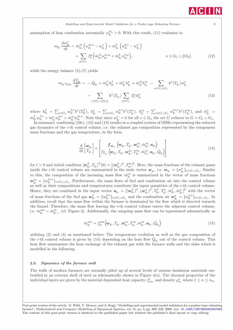
Modelling and Experimental Model Validation for a Pusher-type Reheating Furnace 9
assumption of lean combustion necessarily wO2gi
> 0. With this result, (11) evaluates to
mgi
dwνgi
dt= min
gi
(win,νgi
−wνgi
)+ mb
gi
(wb,νgi
− wνgi
)
+∑
µ∈Go
βµν
(min
giwin,µgi
+ mbgiwb,µgi
), ν ∈ Ge ∪ {O2} (12)
while the energy balance (5)-(7) yields
mgicp,gi
dTgi
dt= − Qgi
+ mfgihfgi
+ magihagi
+ mingihingi
−∑
ν∈Ge∪Ga
hν(Tgi)wν
gi
−∑
ν∈Ge∪{O2}hν(Tgi
)∑
µ∈Go
βµν w
µgi
(13)
where hfgi =∑
ν∈Gfwf,νgi hν(T f
gi), hagi=∑
ν∈Gawa,νgi hν(T a
gi), hingi
=∑
ν∈Ge∪Gawin,νgi hν(T in
gi), and wν
gi=
mfgiw
f,νgi + ma
giwa,νgi + min
giwin,νgi . Note that since wν
gi= 0 for all ν ∈ Go the set G reduces to G = Ge ∪Ga.
In summary, combining (10c), (12) and (13) results in a coupled system of ODEs representing the reducedgas dynamics of the i-th control volume, i.e. the exhaust gas composition represented by the componentmass fractions and the gas temperature, in the form
d
dt
[wgi
Tgi
]=
fwgi
(wgi
, Tgi,win
gi, min
gi,ugi
)
fTgi
(wgi
, Tgi,win
gi, T in
gi, min
gi,ugi
, Qgi
)
(14)
for t > 0 and initial condition [wTgi, Tgi
]T (0) = [(w0gi)T , T 0
gi]T . Here, the mass fractions of the exhaust gases
inside the i-th control volume are summarized in the state vector wgi, i.e. wgi
= {wνgi}ν∈Ge∪Ga
. Similar
to this, the composition of the incoming mass flow mingi
is summarized in the vector of mass fractions
wingi
= {win,νgi }ν∈Ge∪Ga
. Furthermore, the mass flows of fuel and combustion air into the control volumeas well as their compositions and temperatures constitute the input quantities of the i-th control volume.
Hence, they are combined in the input vector ugi= [(wf
gi)T , (wa
gi)T , T f
gi , Tagi, mf
gi , magi]T with the vector
of mass fractions of the fuel gas wfgi = {wf,ν
gi }ν∈Ge∪Gaand the combustion air wa
gi= {wa,ν
gi }ν∈Ge∪Ga. In
addition, recall that the mass flow within the furnace is dominated by the flow which is directed towardsthe funnel. Therefore, the mass flow leaving the i-th control volume enters the adjacent control volume,i.e. mout
gi= min
gi−1(cf. Figure 3). Additionally, the outgoing mass flow can be represented schematically as
moutgi
= f outgi
(wgi
, Tgi,win
gi, T in
gi, min
gi,ugi
, Qgi
)(15)
utilizing (2) and (4) as mentioned before. The temperature evolution as well as the gas composition ofthe i-th control volume is given by (14) depending on the heat flow Qgi
out of the control volume. Thisheat flow summarizes the heat exchange of the exhaust gas with the furnace walls and the slabs which ismodelled in the following.
2.3. Dynamics of the furnace wall
The walls of modern furnaces are normally piled up of several levels of various insulation materials em-bedded in an exterior shell of steel as schematically shown in Figure 4(a). The thermal properties of theindividual layers are given by the material dependent heat capacity cnp,wi
and density ρnwiwhere 1 ≤ n ≤ nwi
Post-print version of the article: D. Wild, T. Meurer, and A. Kugi, “Modelling and experimental model validation for a pusher-type reheatingfurnace”, Mathematical and Computer Modelling of Dynamical Systems, vol. 15, no. 3, pp. 209–232, 2009. doi: 10.1080/13873950902927683The content of this post-print version is identical to the published paper but without the publisher’s final layout or copy editing.

March 1, 2009 12:31 Mathematical and Computer Modelling of Dynamical Systems mcmds˙wild˙08
10 D. Wild, T. Meurer, and A. Kugi
ρ1wi, c1p,wi
ρ2wi, c2p,wi
...
ρnwiwi , c
nwip,wi
�
6
Twi
dwi
r
r To��
(a) Temperature evolution in the multi-layered in-sulation.
ρwi, cp,wi
λwi
�
6
Twi
dwi
dwi
r
r To��
(b) Approximation by a two-layered wall elementwith dwi denoting the effective height of the innerlayer. The outer wall temperature To is measured.
Figure 4. Modelling of the furnace wall wi in the i-th control volume.
indicates the respective layer. In order to model the temperature distribution in the furnace wall the con-vective as well as conductive heat transfer mechanisms have to be considered [14]. However, since on theone hand the convective flow in the furnace is hardly accessible due to the complex furnace dynamics andgeometry and on the other hand the conductive properties of the multiple insulation layers are mainlyunknown, an adapted model has to be derived, which captures the essential thermal dynamics.For this, detailed simulation studies in comparison with measurement campaigns have shown that the
wall temperature mainly varies in a rather thin boundary layer neighbouring the gaseous space followed byan almost linear decrease to the outer wall temperature. As a result, in the following the multi–layered wallof area Awi
and thickness dwisurrounding the i-th control volume is represented by a two–layered element
as depicted in Figure 4(b). The balance of energy for the inner layer of effective thickness dwi≪ dwi
, meandensity ρwi
and mean specific heat capacity cp,wireads as
d
dtTwi
=Qwi
− Qoutwi
cp,wiρwi
Awidwi
, (16)
with the heat flow Qwientering the wall and Qout
withe heat flow to the outer layer. Note that the description
of the heat flow Qwiis postponed to Section 3, where heat radiation in the furnace as the major mode
of heat exchange between the gaseous phase, the slabs, and the walls is discussed in detail. The heat flowQout
widue to heat conduction follows as
Qoutwi
=λwi
Awi
dwi− dwi
(Twi
− To
), (17)
where λwidenotes the average thermal conductivity of the outer layer and To represents the outer wall
temperature [14,15]. It should be pointed out, that To is measured in the considered furnace set-up whilethe parameters dwi
≪ dwi, ρwi
, cp,wi, and λwi
are identified from experimental data.Besides the balance equations for the gaseous furnace space and the surrounding furnace walls, the
modelling of the slabs is of crucial importance.
2.4. Dynamics of the slabs
In pusher-type furnaces, the slab movement in the z-direction is realized by hydraulic pushers, whichdiscontinuously feed new slabs to the furnace. This results in a sliding of the adjoining slabs along theinstalled skid system as depicted in Figure 5.
Post-print version of the article: D. Wild, T. Meurer, and A. Kugi, “Modelling and experimental model validation for a pusher-type reheatingfurnace”, Mathematical and Computer Modelling of Dynamical Systems, vol. 15, no. 3, pp. 209–232, 2009. doi: 10.1080/13873950902927683The content of this post-print version is identical to the published paper but without the publisher’s final layout or copy editing.

March 1, 2009 12:31 Mathematical and Computer Modelling of Dynamical Systems mcmds˙wild˙08
Modelling and Experimental Model Validation for a Pusher-type Reheating Furnace 11
Qsj ,u
Qsj ,d
Tsj ,1
Tsj ,Nsj
xz
y = 0
y = Lysj
skidskid
slab sj
Figure 5. Schematic drawing of the j-th slab, the vertical discretization and the heat flow into the upper and lower surfaces of the slab.
From an energetic point of view, the skids induce a complex temperature distribution in the slab, whichcan be mathematically recovered only by considering 2- (along the (x, y)-directions) or 3-dimensional slabmodels, see, e.g., [16]. However, a detailed slab model results in a dramatic increase in the dimension ofthe system states and thus cannot be used in a real–time environment. Furthermore, in view of processcontrol no active control of the slab temperature in the neighbourhood of the skids is available, such thatin the sequel the analysis is restricted to a 1-dimensional slab model assuming a homogeneous temperaturedistribution in the x- and z-direction. In addition, it is assumed that the heat exchange occurs mainlythrough the upper and lower surfaces of the slabs. Note that these assumptions are in good agreementwith the available measurement data (cf. Section 5). Hence, the temperature distribution Tsj = Tsj(t, y)of the j-th slab sj can be represented by the 1-dimensional heat equation [14], i.e.
cp,sj(Tsj )ρsj(Tsj )∂Tsj
∂t=
∂
∂y
(λsj(Tsj )
∂Tsj
∂y
)(18)
with the temperature dependent parameters for the specific heat capacity cp,sj , the density ρsj , and thethermal conductivity λsj of the respective steel alloy [17]. The boundary conditions follow as
λsj(Tsj)∂Tsj
∂y= −Qsj,d
Asj
at y = 0 (19a)
λsj(Tsj)∂Tsj
∂y=
Qsj ,u
Asj
at y = Lysj . (19b)
Here Qsj,d and Qsj ,u denote the heat flows into the slab sj at the upper and lower slab surface Asj , whichdepend on the properties of the surrounding gas and the neighbouring furnace walls due to the dominatingradiative heat exchange. A detailed derivation of the respective expressions for Qsj ,d and Qsj ,u is given inSection 3. The corresponding initial conditions read as
Tsj(t0, y) = T 0sj(y), y ∈ [0, Ly
sj ]. (20)
with t0 ≥ 0 as the charging time of the respective slab.In order to obtain a model suitable for real-time applications the governing heat equation (18) and the
corresponding boundary conditions (19) are semi-discretized using the finite difference method [14, 18].This results in a system of Nsj nonlinear ODEs
d
dtT sj = f sj
(T sj , Qsj ,d, Qsj ,u
)(21a)
for t > t0 with the initial condition T sj(t0) = T 0sj due to (20). Thus, a nonlinear system of ODEs with the
state vector T sj(t) = [Tsj ,1, . . . , Tsj ,Nsj]T of discrete slab temperatures along the slab height as depicted
in Figure 5 is obtained for each slab. The following section is devoted to the derivation of the heat flowsQsj,u and Qsj ,d as well as of the heat flows into the furnace walls Qwi
and out of the exhaust gas Qgi.
Post-print version of the article: D. Wild, T. Meurer, and A. Kugi, “Modelling and experimental model validation for a pusher-type reheatingfurnace”, Mathematical and Computer Modelling of Dynamical Systems, vol. 15, no. 3, pp. 209–232, 2009. doi: 10.1080/13873950902927683The content of this post-print version is identical to the published paper but without the publisher’s final layout or copy editing.
March 1, 2009 12:31 Mathematical and Computer Modelling of Dynamical Systems mcmds˙wild˙08
12 D. Wild, T. Meurer, and A. Kugi
3. Heat radiation within the furnace
In the previous section, dynamical models are determined for the exhaust gas composition and the exhaustgas temperature as well as for the wall and the slab temperature distributions. Herein, the heat flowsentering or leaving the sub-models are represented schematically by the variables Qgi
, Qwi, Qsj ,u, and
Qsj,d. Basically, these heat flows are caused by an energy exchange between the exhaust gas, the walls andthe slabs. Since the pusher-type furnace is normally operated at temperatures above 1000◦C, radiative heatexchange is considered as the major mode of heat exchange such that convective heat exchange between thegas phase and the wall and the slab surfaces can be neglected. Next the radiative heat transfer mechanismsinside a fuel fired furnace will be briefly outlined followed by the determination of the heat flows Qgi
, Qwi,
Qsj,u, and Qsj,d.
3.1. Radiating properties
For the subsequent derivations solid body and gas radiation have to be distinguished. Thereby, the solidsurfaces of the furnace walls and the slabs are considered as diffuse, opaque, and grey radiators. Theemissivity of solid surfaces depends among others on the surface temperature, the material, and the surfacetexture. For the slabs the latter is affected by the proceeding surface oxidization during the reheatingprocess1, which significantly complicates the determination of the emissivity of the slabs or makes it evenimpossible. Hence, in the following an empirical surface temperature dependent emissivity εsj (Tsj ,1) andεsj(Tsj ,Nsj
) is presumed. Since the temperature of the furnace walls only varies in a small temperaturerange the emissivity of the furnace walls εwi
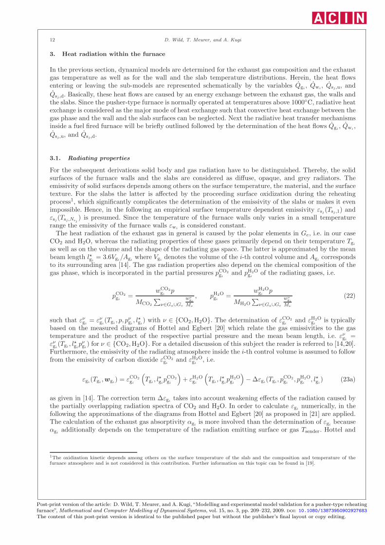
is considered constant.The heat radiation of the exhaust gas in general is caused by the polar elements in Ge, i.e. in our case
CO2 and H2O, whereas the radiating properties of these gases primarily depend on their temperature Tgi
as well as on the volume and the shape of the radiating gas space. The latter is approximated by the meanbeam length l⋆gi
= 3.6Vgi/Agi
where Vgidenotes the volume of the i-th control volume and Agi
correspondsto its surrounding area [14]. The gas radiation properties also depend on the chemical composition of thegas phase, which is incorporated in the partial pressures pCO2
giand pH2O
giof the radiating gases, i.e.
pCO2
gi=
wCO2gi
p
MCO2
∑ν∈Ga∪Ge
wνgi
Mν
, pH2Ogi
=wH2Ogi
p
MH2O∑
ν∈Ga∪Ge
wνgi
Mν
(22)
such that ενgi= ενgi
(Tgi, p, pνgi
, l⋆gi) with ν ∈ {CO2,H2O}. The determination of εCO2
giand εH2O
giis typically
based on the measured diagrams of Hottel and Egbert [20] which relate the gas emissivities to the gastemperature and the product of the respective partial pressure and the mean beam length, i.e. ενgi
=ενgi
(Tgi, l⋆gi
pνgi) for ν ∈ {CO2,H2O}. For a detailed discussion of this subject the reader is referred to [14,20].
Furthermore, the emissivity of the radiating atmosphere inside the i-th control volume is assumed to followfrom the emissivity of carbon dioxide εCO2
giand εH2O
gi, i.e.
εgi(Tgi
,wgi) = εCO2
gi
(Tgi
, l⋆gipCO2
gi
)+ εH2O
gi
(Tgi
, l⋆gipH2Ogi
)−∆εgi
(Tgi, pCO2
gi, pH2O
gi, l⋆gi
) (23a)
as given in [14]. The correction term ∆εgitakes into account weakening effects of the radiation caused by
the partially overlapping radiation spectra of CO2 and H2O. In order to calculate εginumerically, in the
following the approximations of the diagrams from Hottel and Egbert [20] as proposed in [21] are applied.The calculation of the exhaust gas absorptivity αgi
is more involved than the determination of εgibecause
αgiadditionally depends on the temperature of the radiation emitting surface or gas Tsender. Hottel and
1The oxidization kinetic depends among others on the surface temperature of the slab and the composition and temperature of thefurnace atmosphere and is not considered in this contribution. Further information on this topic can be found in [19].
Post-print version of the article: D. Wild, T. Meurer, and A. Kugi, “Modelling and experimental model validation for a pusher-type reheatingfurnace”, Mathematical and Computer Modelling of Dynamical Systems, vol. 15, no. 3, pp. 209–232, 2009. doi: 10.1080/13873950902927683The content of this post-print version is identical to the published paper but without the publisher’s final layout or copy editing.
March 1, 2009 12:31 Mathematical and Computer Modelling of Dynamical Systems mcmds˙wild˙08
Modelling and Experimental Model Validation for a Pusher-type Reheating Furnace 13
T sj T sj−1T sj+1
x
y
z
Tgi
Tgi+1
Tgi−1
TwiTwi−1
Twi+1
EwiAwi Jwi
Awi
EisjA
isjJ
isjA
isj
A+gi
A−gi
Aisj+1
Ai+1sj+1
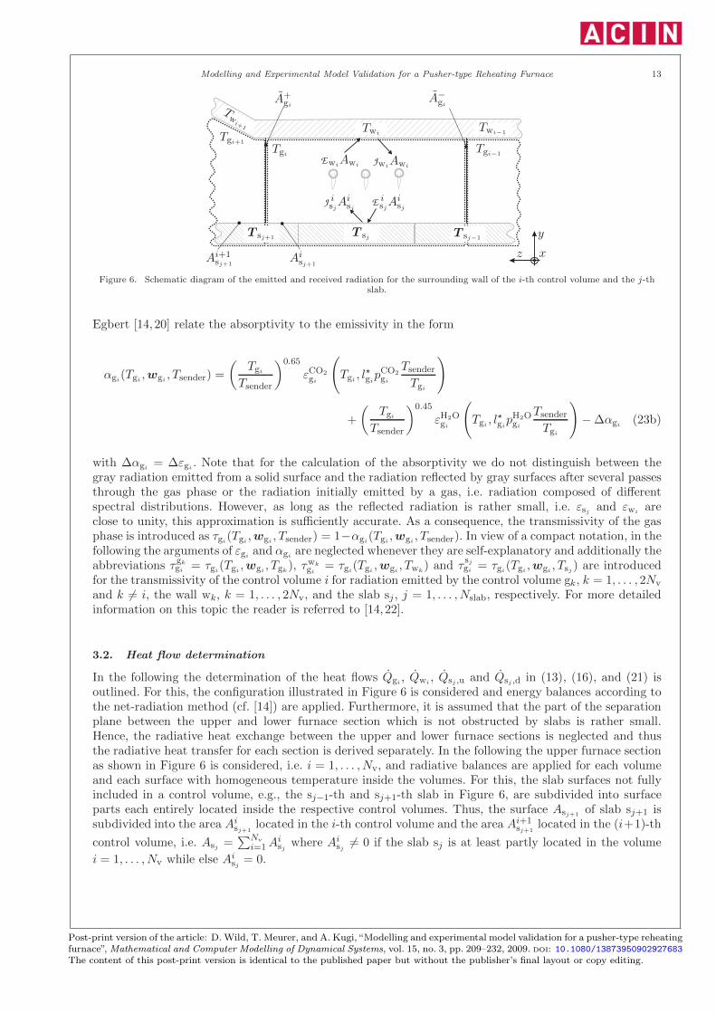
Figure 6. Schematic diagram of the emitted and received radiation for the surrounding wall of the i-th control volume and the j-thslab.
Egbert [14,20] relate the absorptivity to the emissivity in the form
αgi(Tgi
,wgi, Tsender) =
(Tgi
Tsender
)0.65
εCO2
gi
(Tgi
, l⋆gipCO2
gi
Tsender
Tgi
)
+
(Tgi
Tsender
)0.45
εH2Ogi
(Tgi
, l⋆gipH2Ogi
Tsender
Tgi
)−∆αgi
(23b)
with ∆αgi= ∆εgi
. Note that for the calculation of the absorptivity we do not distinguish between thegray radiation emitted from a solid surface and the radiation reflected by gray surfaces after several passesthrough the gas phase or the radiation initially emitted by a gas, i.e. radiation composed of differentspectral distributions. However, as long as the reflected radiation is rather small, i.e. εsj and εwi
areclose to unity, this approximation is sufficiently accurate. As a consequence, the transmissivity of the gasphase is introduced as τgi
(Tgi,wgi
, Tsender) = 1−αgi(Tgi
,wgi, Tsender). In view of a compact notation, in the
following the arguments of εgiand αgi
are neglected whenever they are self-explanatory and additionally theabbreviations τgk
gi = τgi(Tgi
,wgi, Tgk
), τwkgi
= τgi(Tgi
,wgi, Twk
) and τsjgi = τgi
(Tgi,wgi
, Tsj ) are introducedfor the transmissivity of the control volume i for radiation emitted by the control volume gk, k = 1, . . . , 2Nv
and k 6= i, the wall wk, k = 1, . . . , 2Nv, and the slab sj , j = 1, . . . , Nslab, respectively. For more detailedinformation on this topic the reader is referred to [14,22].
3.2. Heat flow determination
In the following the determination of the heat flows Qgi, Qwi
, Qsj ,u and Qsj ,d in (13), (16), and (21) isoutlined. For this, the configuration illustrated in Figure 6 is considered and energy balances according tothe net-radiation method (cf. [14]) are applied. Furthermore, it is assumed that the part of the separationplane between the upper and lower furnace section which is not obstructed by slabs is rather small.Hence, the radiative heat exchange between the upper and lower furnace sections is neglected and thusthe radiative heat transfer for each section is derived separately. In the following the upper furnace sectionas shown in Figure 6 is considered, i.e. i = 1, . . . , Nv, and radiative balances are applied for each volumeand each surface with homogeneous temperature inside the volumes. For this, the slab surfaces not fullyincluded in a control volume, e.g., the sj−1-th and sj+1-th slab in Figure 6, are subdivided into surfaceparts each entirely located inside the respective control volumes. Thus, the surface Asj+1
of slab sj+1 issubdivided into the area Ai
sj+1located in the i-th control volume and the area Ai+1
sj+1located in the (i+1)-th
control volume, i.e. Asj =∑Nv
i=1Aisj where Ai
sj 6= 0 if the slab sj is at least partly located in the volume
i = 1, . . . , Nv while else Aisj = 0.
Post-print version of the article: D. Wild, T. Meurer, and A. Kugi, “Modelling and experimental model validation for a pusher-type reheatingfurnace”, Mathematical and Computer Modelling of Dynamical Systems, vol. 15, no. 3, pp. 209–232, 2009. doi: 10.1080/13873950902927683The content of this post-print version is identical to the published paper but without the publisher’s final layout or copy editing.

March 1, 2009 12:31 Mathematical and Computer Modelling of Dynamical Systems mcmds˙wild˙08
14 D. Wild, T. Meurer, and A. Kugi
Energy balancing for the wall wi and the slab sj, respectively, yields
Qwi= Ewi
Awi− Jwi
Awi, Qsj,u =
Nv∑
i=1
(EisjA
isj − J isjAi
sj
), (24)
where EwiAwi
and E isjAisj denote the irradiance received by the surfaces Awi
and Aisj while Jwi
Awiand
JisjA
isj are called the radiosity of the surfaces Awi
and Aisj , respectively. Furthermore, the radiosity is
composed of the emissive power of the respective surface and the portion of reflected irradiance, i.e.
JwiAwi
= σεwiAwi
T 4wi
+ (1− εwi) Ewi
Awi(25a)
JisjA
isj = σεsjA
isjT
4sj ,Nsj
+(1− εsj
)EisjA
isj (25b)
with σ the Stefan–Boltzmann constant (cf. [14]). The irradiance is represented by the received radiosityof all surfaces in the upper furnace section and the emissive power of the gas volumes weighted with therespective transmissivity, i.e.
EwiAwi
=
Nv∑
k=1
[Jwk
AwkFAwk
,Awiτwk
k,i + σεgkκAwi
,gk
i,k T 4gk
+
Nslab∑
j=1
JksjA
ksjFAk
sj,Awi
τsjk,i
](26a)
EisjA
isj =
Nv∑
k=1
[Jwk
AwkFAwk
,Aisjτwk
k,i + σεgkκAk
sj,gk
i,k T 4gk
]. (26b)
Thereby, the orientation of the surfaces A1 and A2 is taken into account by the so-called view factorFA1,A2
relating the portion of the radiosity emitted by the surface A1 being received by the surface A2
(cf. [14]). Assuming planar surfaces, the view factors can easily be calculated using the algorithms presentedin [22,23]. Additionally, the abbreviations
τ ιk,i =
∏i=k τ
ιg
for i > k
τ ιgifor i = k∏k
=i τιg
for i < k
and κζ,ξi,k =
A−gkFA−
gk,ζ τ
ξi,k−1 for i < k
ζ for i = k
A+gkFA+
gk,ζ τ
ξi,k+1 for i > k
(27)
are introduced, where τ ιk,i combines the transmissivity of the gas volumes gk to gi due to the radiosity of
ι. Note that A+gi
and A−gi
denote the surface of the separation planes between the i-th gas volume and theadjacent gas volumes on the left and on the right, respectively (cf. Figure 6). By balancing the emissivepower and the absorbed irradiation of the i-th gas volume, the outgoing heat flow Qgi
follows as
Qgi= σεgi
AgiT 4gi−
Nv∑
k=1
Jwk
κAwk
,wk
k,i αwk
gi+
Nslab∑
j=1
Jksjκ
Aksj,sj
k,i αsjgi+ (1− δi,k)σεgk
αgk
giκAsign(i−k)
gk,gk
k+sign(i−k),iT4gk
(28)
with the Kronecker delta δi,i = 1 while δi,k = 0, i 6= k and the signum function sign (i). In order todetermine the radiosities Jwi
and J isj for i = 1, . . . , Nv, j = 1, . . . , Nslab, a linear system of equationsis obtained by considering (25) with (26) for i = 1, . . . , Nv, j = 1, . . . , Nslab. Furthermore, due to theabsorption of the exhaust gas, it makes sense to limit the radiative exchange to adjacent volumes, i.e. tolimit the summations in (26) and (28) to i− 1 ≤ k ≤ i+ 1. This finally allows to compute the remainingheat flows Qsj,u, Qwi
and Qgiof the upper control volumes, walls, and slab surfaces from (24) and (28).
Due to the assumption of negligible radiative coupling of the upper and lower furnace sections the heat
Post-print version of the article: D. Wild, T. Meurer, and A. Kugi, “Modelling and experimental model validation for a pusher-type reheatingfurnace”, Mathematical and Computer Modelling of Dynamical Systems, vol. 15, no. 3, pp. 209–232, 2009. doi: 10.1080/13873950902927683The content of this post-print version is identical to the published paper but without the publisher’s final layout or copy editing.
March 1, 2009 12:31 Mathematical and Computer Modelling of Dynamical Systems mcmds˙wild˙08
Modelling and Experimental Model Validation for a Pusher-type Reheating Furnace 15
flows Qsj ,d, Qwiand Qgi
in the lower furnace section are calculated similarly for i = Nv + 1, . . . , 2Nv andthe lower slab temperatures Tsj ,1. The major difference between the furnace sections is the installed skidsystem consisting of insulated but internally cooled pipes on which the slabs are sliding (cf. Figures 1and 6). These skids partly obstruct the radiating surfaces, which can be incorporated in the calculationof the respective view factors of the slabs and their environment. Unfortunately, no data is available toidentify the spatial cooling characteristics of the skids inside the furnace. Thus, the overall amount of heatdissipated by the skid system is prorated to the lower control volumes and the lower walls. The feasibility ofthis simplification is shown in Section 5 where the good agreement of simulation results and measurementdata are discussed.
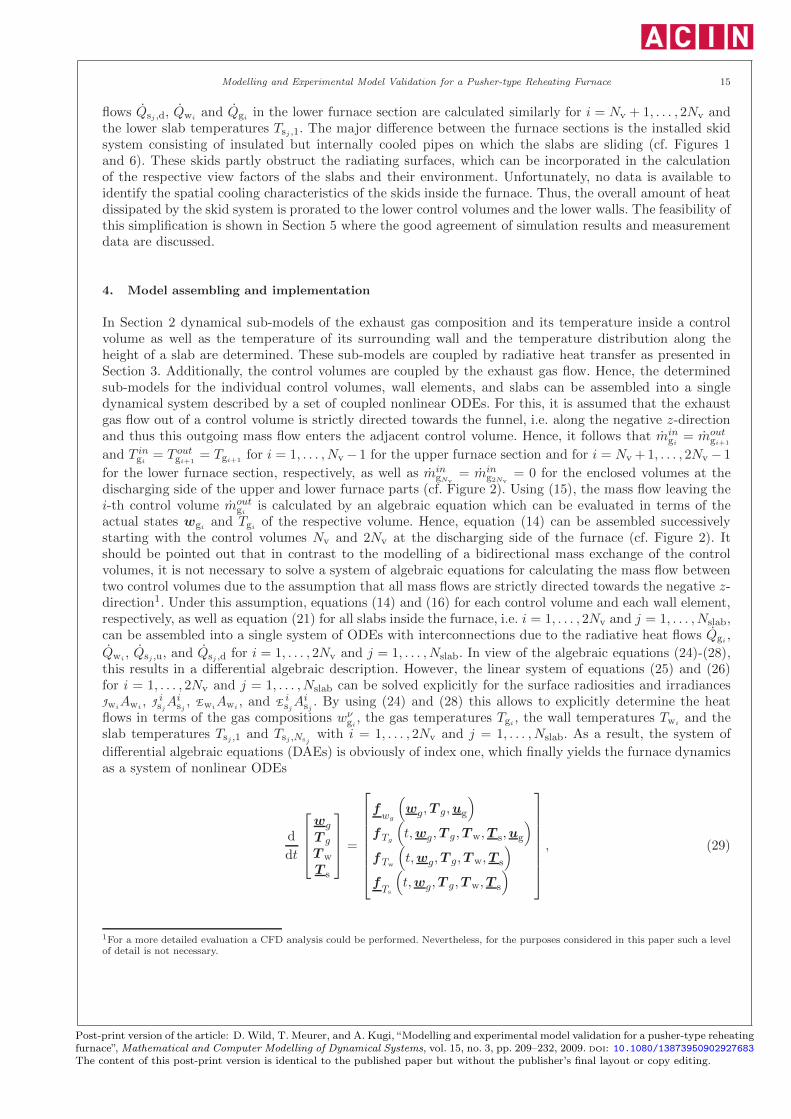
4. Model assembling and implementation
In Section 2 dynamical sub-models of the exhaust gas composition and its temperature inside a controlvolume as well as the temperature of its surrounding wall and the temperature distribution along theheight of a slab are determined. These sub-models are coupled by radiative heat transfer as presented inSection 3. Additionally, the control volumes are coupled by the exhaust gas flow. Hence, the determinedsub-models for the individual control volumes, wall elements, and slabs can be assembled into a singledynamical system described by a set of coupled nonlinear ODEs. For this, it is assumed that the exhaustgas flow out of a control volume is strictly directed towards the funnel, i.e. along the negative z-directionand thus this outgoing mass flow enters the adjacent control volume. Hence, it follows that min
gi= mout
gi+1
and T ingi
= T outgi+1
= Tgi+1for i = 1, . . . , Nv − 1 for the upper furnace section and for i = Nv +1, . . . , 2Nv − 1
for the lower furnace section, respectively, as well as mingNv
= ming2Nv
= 0 for the enclosed volumes at thedischarging side of the upper and lower furnace parts (cf. Figure 2). Using (15), the mass flow leaving thei-th control volume mout
giis calculated by an algebraic equation which can be evaluated in terms of the
actual states wgiand Tgi
of the respective volume. Hence, equation (14) can be assembled successivelystarting with the control volumes Nv and 2Nv at the discharging side of the furnace (cf. Figure 2). Itshould be pointed out that in contrast to the modelling of a bidirectional mass exchange of the controlvolumes, it is not necessary to solve a system of algebraic equations for calculating the mass flow betweentwo control volumes due to the assumption that all mass flows are strictly directed towards the negative z-direction1. Under this assumption, equations (14) and (16) for each control volume and each wall element,respectively, as well as equation (21) for all slabs inside the furnace, i.e. i = 1, . . . , 2Nv and j = 1, . . . , Nslab,can be assembled into a single system of ODEs with interconnections due to the radiative heat flows Qgi
,
Qwi, Qsj ,u, and Qsj ,d for i = 1, . . . , 2Nv and j = 1, . . . , Nslab. In view of the algebraic equations (24)-(28),
this results in a differential algebraic description. However, the linear system of equations (25) and (26)for i = 1, . . . , 2Nv and j = 1, . . . , Nslab can be solved explicitly for the surface radiosities and irradiancesJwi
Awi, J isjA
isj , Ewi
Awi, and E isjA
isj . By using (24) and (28) this allows to explicitly determine the heat
flows in terms of the gas compositions wνgi, the gas temperatures Tgi
, the wall temperatures Twiand the
slab temperatures Tsj ,1 and Tsj ,Nsjwith i = 1, . . . , 2Nv and j = 1, . . . , Nslab. As a result, the system of
differential algebraic equations (DAEs) is obviously of index one, which finally yields the furnace dynamicsas a system of nonlinear ODEs
d
dt
wg
T g
Tw
T s
=
fwg
(wg,T g,ug
)
fTg
(t,wg,T g,Tw,T s,ug
)
fTw
(t,wg,T g,Tw,T s
)
fTs
(t,wg,T g,Tw,T s
)
, (29)
1For a more detailed evaluation a CFD analysis could be performed. Nevertheless, for the purposes considered in this paper such a levelof detail is not necessary.
Post-print version of the article: D. Wild, T. Meurer, and A. Kugi, “Modelling and experimental model validation for a pusher-type reheatingfurnace”, Mathematical and Computer Modelling of Dynamical Systems, vol. 15, no. 3, pp. 209–232, 2009. doi: 10.1080/13873950902927683The content of this post-print version is identical to the published paper but without the publisher’s final layout or copy editing.

March 1, 2009 12:31 Mathematical and Computer Modelling of Dynamical Systems mcmds˙wild˙08
16 D. Wild, T. Meurer, and A. Kugi
with the vector wg = {wgi}i=1,...,2Nv
and the vector T g = {Tgi}i=1,...,2Nv
composed of the mass fractionvectors of all control volumes and the gas temperatures inside all volumes, respectively. The vector Tw ={Twi
}i=1,...,2Nvcombines the temperatures of all walls and T s = {T sj}j=1,...,Nslab
is composed of all slabtemperature vectors. Similarly to the state variables on the left hand side of (29), the functions on the righthand side are composed of the respective right hand sides of the sub-model ODEs. In detail, the vectorfwg
= {fwgi}i=1,...,2Nv
and the vector fTg= {fTgi
}i=1,...,2Nvare given by the right hand sides of (14) for
all control volumes and the vector fTwis composed of the right hand side of (16) for all walls. Finally,
the vector fTs
= {f sj}j=1,...,Nslabconsists of the right hand side of (21) for all slabs inside the furnace.
The input variables of the ODEs (29) follow as ug = {ugi}i=1,...,2Nv
, which combines the input variablesof all indivdual control volumes. In summary, (29) represents the dominating dynamics of the consideredpusher-type reheating furnace. Furthermore, recall that the pusher-type reheating furnace can be classifiedas a hybrid system due to the event driven slab movements as well as the charging and discharging processwhich is expressed in (29) by the explicit dependence on the time t of the functions on the right hand side.In addition, whenever slabs are charged or discharged the dimensions of T s and f
Tsin (29) have to be
adapted such that the dimension of the overall system (29) given as 2Nv(dim(Ge ∪Ga) + 2) +∑Nslab
j=1 Nsj
in a typical operation mode varies approximately between 270 and 360.For the numerical solution the set of ODEs (29) is implemented in Matlab/Simulink. Therefore,
the sub-models presented in Section 2 are implemented using the programming language C++. Thisallows to examine several furnace configurations with only small changes of the source code. In addition,this ensures simple portability of the implementation to the automation system of the plant. During thenumerical solution the differential equations (29) are successively re-assembled and re-adapted accordingto the current charging situation inside the furnace. This includes the recurrent change of the modeldimension.
5. Experimental model validation
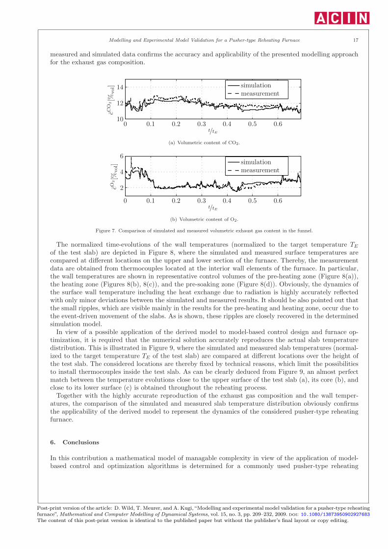
In order to validate the developed mathematical model (29) a measurement campaign was performed at theAG der Dillinger Huttenwerke in Dillingen, Germany. Therefore, a test slab equipped with thermocoupleswas reheated in the pusher-type reheating furnace schematically illustrated in Figure 1. Besides the alreadymentioned temperature measurement of the test slab, the wall surface temperatures and the exhaust gascompositions inside the funnel are additionally measured. Furthermore, the input variables ug, i.e. themass flows of fuel and combustion air as well as their temperature are measured and are used as inputsfor the numerical solution of (29) with a furnace discretization of Nv = 10. Note that subsequentiallyall quantities are depicted in a normalized fashion with the time variable scaled by the duration of themeasurement campaign tE .At first, a comparison of the simulated and measured exhaust gas composition is illustrated in Figure
7 where the normalized time-evolutions of the concentrations of CO2 and O2 inside the funnel are shown,respectively. Note that the depicted volumetric exhaust gas composition cν , ν ∈ {CO2,O2} inside thefunnel can be easily obtained by considering the mixture of the mass flows mout
g1and mout
gNv+1, i.e.
cCO2 =wCO2
f
MCO2
∑ν∈Ga∪Ge
wνf
Mν
, cO2 =wO2
f
MO2
∑ν∈Ga∪Ge
wνf
Mν
(30)
with the mass fractions of the exhaust gas flow in the funnel
wνf =
moutg1
wνg1
+ moutgNv+1
wνgNv+1
moutg1
+ moutgNv+1
, ν ∈ Ga ∪Ge.
Unfortunately, due to an unrecoverable failure of the corresponding measurement devices during the ex-periment, the time axis in Figure 7 is truncated at t/tE ≈ 0.7. Nevertheless, the superior agreement of
Post-print version of the article: D. Wild, T. Meurer, and A. Kugi, “Modelling and experimental model validation for a pusher-type reheatingfurnace”, Mathematical and Computer Modelling of Dynamical Systems, vol. 15, no. 3, pp. 209–232, 2009. doi: 10.1080/13873950902927683The content of this post-print version is identical to the published paper but without the publisher’s final layout or copy editing.
March 1, 2009 12:31 Mathematical and Computer Modelling of Dynamical Systems mcmds˙wild˙08
Modelling and Experimental Model Validation for a Pusher-type Reheating Furnace 17
measured and simulated data confirms the accuracy and applicability of the presented modelling approachfor the exhaust gas composition.
0 0.1 0.2 0.3 0.4 0.5 0.610
12
14
t/tE
cCO
2[%
vol] simulation
measurement
(a) Volumetric content of CO2.
0 0.1 0.2 0.3 0.4 0.5 0.6
2
4
6
t/tE
cO2[%
vol] simulation
measurement
(b) Volumetric content of O2.
Figure 7. Comparison of simulated and measured volumetric exhaust gas content in the funnel.
The normalized time-evolutions of the wall temperatures (normalized to the target temperature TE
of the test slab) are depicted in Figure 8, where the simulated and measured surface temperatures arecompared at different locations on the upper and lower section of the furnace. Thereby, the measurementdata are obtained from thermocouples located at the interior wall elements of the furnace. In particular,the wall temperatures are shown in representative control volumes of the pre-heating zone (Figure 8(a)),the heating zone (Figures 8(b), 8(c)), and the pre-soaking zone (Figure 8(d)). Obviously, the dynamics ofthe surface wall temperature including the heat exchange due to radiation is highly accurately reflectedwith only minor deviations between the simulated and measured results. It should be also pointed out thatthe small ripples, which are visible mainly in the results for the pre-heating and heating zone, occur due tothe event-driven movement of the slabs. As is shown, these ripples are closely recovered in the determinedsimulation model.In view of a possible application of the derived model to model-based control design and furnace op-
timization, it is required that the numerical solution accurately reproduces the actual slab temperaturedistribution. This is illustrated in Figure 9, where the simulated and measured slab temperatures (normal-ized to the target temperature TE of the test slab) are compared at different locations over the height ofthe test slab. The considered locations are thereby fixed by technical reasons, which limit the possibilitiesto install thermocouples inside the test slab. As can be clearly deduced from Figure 9, an almost perfectmatch between the temperature evolutions close to the upper surface of the test slab (a), its core (b), andclose to its lower surface (c) is obtained throughout the reheating process.Together with the highly accurate reproduction of the exhaust gas composition and the wall temper-
atures, the comparison of the simulated and measured slab temperature distribution obviously confirmsthe applicability of the derived model to represent the dynamics of the considered pusher-type reheatingfurnace.
6. Conclusions
In this contribution a mathematical model of managable complexity in view of the application of model-based control and optimization algorithms is determined for a commonly used pusher-type reheating
Post-print version of the article: D. Wild, T. Meurer, and A. Kugi, “Modelling and experimental model validation for a pusher-type reheatingfurnace”, Mathematical and Computer Modelling of Dynamical Systems, vol. 15, no. 3, pp. 209–232, 2009. doi: 10.1080/13873950902927683The content of this post-print version is identical to the published paper but without the publisher’s final layout or copy editing.

March 1, 2009 12:31 Mathematical and Computer Modelling of Dynamical Systems mcmds˙wild˙08
18 D. Wild, T. Meurer, and A. Kugi
0 0.2 0.4 0.6 0.8 1
0.7
0.8
0.9
1
t/tETw4/T
E
simulationmeasurement
(a) Temperature Tw4 of a wall element located in the pre-heating zone of the upper furnace section.
0 0.2 0.4 0.6 0.8 1
0.8
0.9
1
1.1
t/tE
Tw7/T
E
simulationmeasurement
(b) Temperature Tw7 of a wall element located in the heating zone of the upper furnace section.
0 0.2 0.4 0.6 0.8 1
0.8
0.9
1
1.1
t/tE
Tw17/T
E
simulationmeasurement
(c) Temperature Tw17 of a wall element located in the heating zone of the lower furnace section.
0 0.2 0.4 0.6 0.8 10.7
0.8
0.9
1
1.1
t/tE
Tw18/T
E
simulationmeasurement
(d) Temperature Tw18 of a wall element located in the pre-soaking zone of the lower furnace section.
Figure 8. Comparison of simulated and measured wall surface temperatures for a representative variety of discretized wall elements inthe pre-heating zone (a), the heating zone (b), (c), and the pre-soaking zone (d). The temperatures are normalized to the target
temperature of the test slab TE .
furnace. Similar to the zone method the furnace is decomposed into suitable control volumes whose upperand lower boundaries are given by the respective furnace walls and the slabs moving through the furnace.Besides the gas dynamics due to combustion and convection, the heat exchange due to radiation betweenthe gaseous phase, the surrounding walls, and the slabs inside the furnace represents the dominatingdynamics of the reheating process.For modelling purposes, at first mass and energy balances are set up for each control volume in order
to capture the combustion process. The complexity of the system description is reduced by applyingthe singular perturbation theory to eliminate the rather fast dynamics of the combustion process. Thedynamics of the surface temperature of the furnace walls is approximated by an ODE taking into accountthe dynamics of a thin inner wall layer and the heat conduction through the outer wall layers. Due to the
Post-print version of the article: D. Wild, T. Meurer, and A. Kugi, “Modelling and experimental model validation for a pusher-type reheatingfurnace”, Mathematical and Computer Modelling of Dynamical Systems, vol. 15, no. 3, pp. 209–232, 2009. doi: 10.1080/13873950902927683The content of this post-print version is identical to the published paper but without the publisher’s final layout or copy editing.

March 1, 2009 12:31 Mathematical and Computer Modelling of Dynamical Systems mcmds˙wild˙08
Modelling and Experimental Model Validation for a Pusher-type Reheating Furnace 19
0 0.2 0.4 0.6 0.8 10
0.5
1
t/tETsj(t,4 5
Ly sj) /TE
simulationmeasurement
(a) Temperature of the test slab near the upper surface at y = 45Lysj .
0 0.2 0.4 0.6 0.8 10
0.5
1
t/tE
Tsj(t,1 2
Ly sj) /TE
simulationmeasurement
(b) Core temperature of the test slab, i.e. y = 12Lysj .
0 0.2 0.4 0.6 0.8 10
0.5
1
t/tE
Tsj(t,1 5
Ly sj) /TE
simulationmeasurement
(c) Temperature of the test slab near the lower surface at y = 15Lysj .
Figure 9. Comparision of simulated and measured normalized temperature distribution of the test slab at certain positions along theslab height.
broad temperature range the temperature distribution in each slab has to be described in terms of theheat equation with temperature-dependent parameters wich is discretized by means of the finite differencemethod.Since the sub-models obtained for each control volume are interconnected by the heat exchange due
radiation, the overall system model is determined in an assembly process by applying the so–called netradiation method. For the numerical simulation the resulting system of ODEs is implemented in Mat-lab/Simulink. Due to the event-driven movement of the slabs, i.e. new slabs can only enter the furnacewhenever reheated slabs are pushed out of the furnace, the system can be classified as a hybrid system. Thissignificantly complicates the implementation because the sub-models have to be re–assembled wheneverslabs enter or leave the furnace due to the changing radiative coupling of the slabs with their environment.In addition, the number of slabs inside the furnace varies, which results in a varying dimension of thesystem model.Besides numerical analysis, the determined model of the reheating process is validated by experimental
results obtained from a measurement campaign with a test slab equipped with thermocouples at the AGder Dillinger Huttenwerke, Dillingen, Germany. The high accuracy of the model is thereby confirmed bycomparing the time-evolutions of the simulated and measured exhaust gas composition, the wall temper-atures as well as the slab temperatures. This in particular emphasizes the applicability of the consideredapproach in view of model-based control and optimization of the furnace operation.
Post-print version of the article: D. Wild, T. Meurer, and A. Kugi, “Modelling and experimental model validation for a pusher-type reheatingfurnace”, Mathematical and Computer Modelling of Dynamical Systems, vol. 15, no. 3, pp. 209–232, 2009. doi: 10.1080/13873950902927683The content of this post-print version is identical to the published paper but without the publisher’s final layout or copy editing.
March 1, 2009 12:31 Mathematical and Computer Modelling of Dynamical Systems mcmds˙wild˙08
20 D. Wild, T. Meurer, and A. Kugi
7. Acknowledgments
The authors would like to thank the AG der Dillinger Huttenwerke for the financial support, the fruitfuldiscussions and in particular for supporting us in successfully accomplishing the measurement campaigns.
References[1] Kim, M., 2007, A heat transfer model for the analysis of transient heating of the slab in a direct-fired walking beam type reheating
furnace. Int. Journal of Heat and Mass Transfer, 50, 2740–2748.[2] Kim, J.G. and Huh, K., 2000, Three-dimensional analysis of the walking-beam-type slab reheating furnace in hot strip mills. Numerical
Heat Transfer, 48, 589–609.[3] Boineau, P., Copin, C. and Aguile, F., 2002, Heat transfer modelling using advanced zone model based on a CFD code. In: Proceedings
of the Proceedings of the 6th European Conference on Industrial Furnaces and Boilers (INFUB), Lisbon, Portugal, pp. 85–94.[4] Hackl, F., 1974, Eine betriebsorientierte Methode zur Berechnung der instationaren thermischen Vorgange in Warmofen. PhD thesis,
Montanuniversitat Leoben.[5] Jaklic, A., Vode, F. and Kolenko, T., 2007, Online simulation model of the slab-reheating process in a pusher-type furnace. Applied
Thermal Engineering, 5-6, 1105–1114.[6] Marino, P.A., Pignotti, A. and Solis, D., 2002, Numerical model of steel slab reheating in pusher furnaces. Latin American Applied
Research, 32(3), 257–261.[7] Cohen, E.S., 1951, Effect of gas temperature gradients on radiant heat transmission. PhD thesis, Massachusetts Institute of Technology.[8] Korndorfer, U., 1975, Mathematisches Modell zur Beschreibung der Warmeubertragung in Stoßofen. PhD thesis, Universitat Karl-
sruhe.[9] Stracke, H., 1979, Der Einfluß der Gasstrahlung auf den Warmeubertrag im Stoßofen - ein mathematisches Modell. PhD thesis,
RWTH Aachen.[10] Rhine, J.M. and Tucker, R.J., 1991 Modelling of gas-fired furnaces and boilers (London, New York: British Gas, McGraw-Hill Book
Company).[11] Turns, S.R., 2000 An Introduction to Combustion, 2 (Boston: McGraw-Hill).[12] Stephan, P., Schaber, K., Stephan, K. and Mayinger, F., 1999 Thermodynamik 2, Mehrstoffsysteme, 14 (Berlin: Springer-Verlag).[13] Khalil, H., 2002 Nonlinear Systems, 3 (New Jersey: Prentice Hall).[14] Baehr, H.D. and Stephan, K., 2006 Heat and Mass Transfer, 2 (Berlin, Heidelberg: Springer).[15] Woelk, G., 1966, Die Bestimmung der Temperatur in einer Ofenwand bei Berucksichtigung temperaturabhangiger Warmeleitfahigkeit.
Gaswarme, 15(5), 138–142.[16] Laturell, E., 1968, Untersuchung der Kuhlwirkung von Stoßofen-Gleitschienen mit Hilfe eines thermoelektrischen Analogiemodells.
PhD thesis, Technische Universitat Clausthal.[17] Harste, K., 1989, Untersuchung zur Schrumpfung und zur Entstehung von mechanischen Spannungen wahrend der Erstarrung und
nachfolgender Abkuhlung zylindrischer Blocke aus Fe-C-Legierungen. PhD thesis, Technische Universitat Clausthal.[18] Thomas, J.W., 1995 Numerical Partial Differential Equations: Finite Difference Methods, no. 22 In: Texts in Applied Mathematics
(New York, Berlin, Heidelberg: Springer-Verlag).[19] Kofstad, P., 1988 High temperature corrosion (London and New York: Elsevier Applied Science).[20] Hottel, H.C. and Egbert, R.B., 1941, The Radiation of Furnace Gases. Trans. of the A.S.M.E., 63, 297–307.[21] Schack, K., 1970, Berechnung der Strahlung von Wasserdampf und Kohlendioxid. Chemie Ingenieur Technik, 42(2), 53–58.[22] Hottel, H.C. and Sarofim, A.F., 1967 Radiative Transfer (New York: McGraw-Hill Book Company).[23] Walton, G.N., 2002, Calculation of Obstructed View Factors by Adaptive Integration. Technical report MD. NISTIR 6925, National
Institute of Standards and Technology (NISTIR), Gaithersburg.
Post-print version of the article: D. Wild, T. Meurer, and A. Kugi, “Modelling and experimental model validation for a pusher-type reheatingfurnace”, Mathematical and Computer Modelling of Dynamical Systems, vol. 15, no. 3, pp. 209–232, 2009. doi: 10.1080/13873950902927683The content of this post-print version is identical to the published paper but without the publisher’s final layout or copy editing.