modelling and forecasting rig rates on the norwegian
TRANSCRIPT

Discussion Papers
Statistics NorwayResearch department
No. 832•December 2015
Terje Skjerpen, Halvor Briseid Storrøsten, Knut Einar Rosendahl and Petter Osmundsen
Modelling and forecasting rig rates on the Norwegian Continental Shelf


Discussion Papers No. 832, December 2015 Statistics Norway, Research Department
Terje Skjerpen, Halvor Briseid Storrøsten, Knut Einar Rosendahl and Petter Osmundsen
Modelling and forecasting rig rates on the Norwegian Continental Shelf
Abstract: Knowledge about rig markets is crucial for understanding the global oil market. In this paper we first develop a simple bargaining model for rig markets. Then we examine empirically the most important drivers for rig rate formation of floaters operating at the Norwegian Continental Shelf in the period 1991q4 to 2013q4. We use reduced form time series models with two equations and report conditional point and bootstrapped interval forecasts for rig rates and capacity utilization. We then consider two alternative simulations to examine how the oil price and remaining petroleum reserves influence rig rate formation of floaters. In the first alternative simulation we assume a relatively high crude oil price equal to 100 USD (2010) per barrel for the entire forecast period, whereas the reference case features the actual oil price with extrapolated values for the last quarters in the forecast period. According to our results, the rig rates will be about 34 percent higher in 2016q4 with the higher oil price. In the second alternative simulation we explore the effects of opening the Barents Sea and areas around Jan Mayen for petroleum activity. This contributes to dampening the fall in the rig rates and capacity utilization over the last part of the forecast period.
Keywords: Rig rates; Capacity utilization; Oil price; Forecasting; Bootstrapping
JEL classification: C32; C51; C53; L71; Q47
Acknowledgements: We are grateful for comments from Anders Rygh Swensen. Any remaining errors and shortcomings are the sole responsibility of the authors. We acknowledge economic support from the Research Counsil of Norway (PETROSAM 2 programme).
Address: Terje Skjerpen, Statistics Norway, Research Department. E-mail: [email protected]
Halvor Briseid Storrøsten, Statistics Norway, Research Department. E-mail: [email protected]
Knut Einar Rosendahl, Norwegian University of Life Sciences, School of Economics and Business and Statistics Norway, Research Department. E-mail: [email protected]
Petter Osmundsen, University of Stavanger, Department of Industrial Economics and Risk Management. Email: [email protected]

Discussion Papers comprise research papers intended for international journals or books. A preprint of a Discussion Paper may be longer and more elaborate than a standard journal article, as it may include intermediate calculations and background material etc.
© Statistics Norway Abstracts with downloadable Discussion Papers in PDF are available on the Internet: http://www.ssb.no/en/forskning/discussion-papers http://ideas.repec.org/s/ssb/dispap.html ISSN 1892-753X (electronic)

3
Sammendrag
Vi analyserer utviklingen i gjennomsnittlige riggrater og kapasitetsutnytting knyttet til virksomheten
på norsk kontinentalsokkel. Vi benytter en to-ligningsmodell spesifisert for kvartalsvise data.
Tidsperioden som betraktes strekker seg fra fjerde kvartal 1991 til utgangen av 2013. I tillegg
rapporterer vi simulerte prediksjoner for den gjennomsnittlige riggraten og kapasitetsutnyttingen for
de 12 påfølgende kvartalene. Ved siden av referansesimuleringen, rapporterer vi også prediksjoner for
to alternative simuleringer. I det første alternativet antar vi en vedvarende høy oljepris svarende til 100
amerikanske dollar i konstante 2010-priser for hele prediksjonsperioden, mens vi i
referansesimuleringen bruker den observerte oljeprisen forlenget med noen fremskrevne verdier.
Ifølge våre resultater ville den gjennomsnittlige riggraten ligge om lag en tredel høyere i fjerde kvartal
2016 ved en vedvarende høy oljepris, sammenlignet med referansesimuleringen. I den andre
alternative simuleringen undersøker vi effekten av å åpne Barentshavet og området rundt Jan Mayen
for petroleumsaktivitet. Økningen i petroleumsreservene som følge av dette bidrar til å dempe fallet i
den gjennomsnittlige riggraten og kapasitetsutnyttingen som forekommer i referansesimuleringen.

4
1. Introduction More than one third of global hydrocarbon supply is extracted offshore and the share is increasing. A
major determinant of offshore hydrocarbon production is the cost of exploration and well
development, where rigs play a key role. Therefore, examining rig markets is crucial for understanding
the global oil market. Moreover, the rig industry itself is a multibillion industry of considerable
interest. In this paper we examine rig rate formation and utilization rates for floaters on the Norwegian
Continental Shelf (NCS). Floaters are rigs that can operate on deep water, and consist of
semisubmersibles and drillships, as opposed to jack-ups that can only operate on more shallow water.
Petroleum activity on the NCS started with the discovery of the Ekofisk field in 1969, one of the
world’s largest offshore oil fields discovered so far. Following Ekofisk was a surge in optimism
regarding the resource potential on the NCS, and during the next two decades major offshore oil and
gas fields were discovered and developed in quick succession.1 In 2014, Norwegian oil and gas
production accounted for, respectively, 2.0 percent and 3.1 percent of global oil and gas production
(BP, 2015), and in 2012 Norway was the 3rd largest exporter of natural gas in the world and the 10th
largest net exporter of oil (Norwegian Petroleum Directorate, 2014).
Petroleum production on the NCS is still dominated by production from the large fields discovered in
the 1970s. As these fields mature, petroleum extraction declines, and total oil production on the NCS
peaked in 2001. The Norwegian government has tried to counteract this development by policies
tailored to spur exploration and development.2 Figure 1 indicates that these policies, along with high
oil prices, have induced more explorative activity on the NCS. The figure also emphasizes two other
interesting points. First, drilling costs constitute a major part of exploration costs. Second, petroleum
exploration has become more costly, partly because the cost of drilling has increased substantially in
recent years. Higher drilling costs are important because drilling affects both the profitability of
existing fields and the cost of exploration.3 While drilling is the major purpose of rig activity, rigs also
provide services such as workovers and plugging during the entire lifetime of an oil and gas field.
1 The fields include, e.g., Statfjord, Troll, Oseberg and Gullfaks, all discovered in the 1970’s. 2 This includes allowance of petroleum activity expansion into new areas such as the southern parts of the Barents Sea. Further, since 2005, companies that are not in a positive tax position can claim reimbursement of the tax value of exploration costs. Recent years have seen major discoveries such as Johan Sverdrup in the North Sea and Johan Castberg in the Barents Sea. 3 The Ministry of Petroleum and Energy (2012, p. 19) estimates that a 30 percent reduction in drilling cost of production and exploration wells from floating platforms will increase the net present value of petroleum resources on the NCS by more than 1000 billion NOK(2012) (172 billion 2012 USD). The estimate is based on an oil price of 90 USD per barrel.

5
Approximately 80 percent of the rig capacity on the NCS in 2011 was used for drilling of new
exploration and production wells (Ministry of Petroleum and Energy, 2012).
Figure 1. Exploration costs (left axis) and number of spudded exploration wells (right axis) on the NCS. Source: Norwegian Petroleum Directorate (http://www.npd.no/en)
Increased offshore exploration costs are not particular for the NCS, see e.g. EIA (2011, p. 111).
Indeed, the cost of drilling has increased worldwide and, as pointed out by Osmundsen et al. (2015),
this cost increase has likely been one of the main factors behind the increase in oil and gas prices over
the last decade. According to Osmundsen et al. (2010a), higher drilling costs observed on the NCS in
the period 2004-2008 were partly due to increased rig rates and partly due to reduced drilling speed.
Moreover, drilling speed tends to be negatively correlated with capacity utilization, due to bottlenecks
and lower drilling quality (Osmundsen et al., 2010b). These features highlight the importance of
understanding rig markets, including rig rates and capacity utilization.
The contribution of the present paper is twofold: The first part is to improve our understanding of rig
markets in general and on the NCS in particular. We present a simple theoretical model to sharpen our
understanding of rig markets and identify the most important drivers for rig rate formation. Then we
estimate their effects based on data for the NCS, and finally we present forecasts for rig rates and
capacity utilization on the NCS. Our second contribution is related to the fact that the rig market data
offer some challenges related to data aggregation and construction of quarterly time series that are of

6
interest from an econometric perspective. For example, we may have several observations (contracts
about future work) of one rig within one quarter.
Our theoretical model solves for the rig rate and hired rig days simultaneously, given demand and
supply for rigs as determined by exogenous variables like the oil price and petroleum resource
potential. The model highlights that an empirical model of the rig market should model both supply
and demand for rigs in order to separate demand and supply side effects. For example, a lower oil
price yields lower expected profitability and, hence, rig demand declines. Keeping rigs idle is very
costly for the rig companies, however, causing aggressive bidding.4 Thus, rig rates will decline, and
exploration, development and new production well drilling become cheaper. This supply side effect
dampens the decline in activity from lower oil price, via lower rig rates.
We then build and estimate a reduced form two-equation econometric model for rig rates and a proxy
for capacity utilization in the NCS rig market for floaters over the period 1990q4 to 2013q4, based on
detailed data on rig contracts and rig characteristics from the shipbroking company Clarksons Platou
Offshore. The two equation framework allows us to account for both supply and demand effects in the
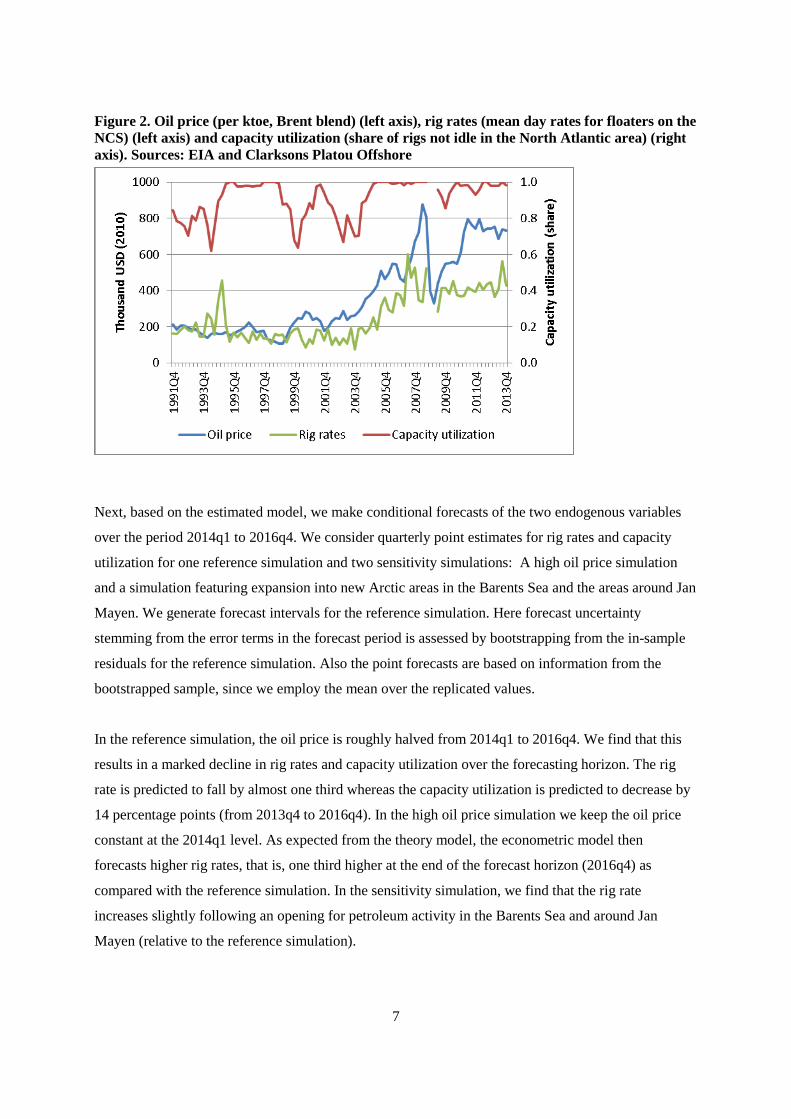
rig market. The two endogenous variables are shown in Figure 2, together with the Brent Blend oil
price. Note that the rig rate series is calculated based on data on individual rig contracts (see Section 3
for details), whereas the capacity utilization series is taken directly from the Clarksons Platou Offshore
data. The figure shows that rig rates are volatile and, not surprisingly, suggests a positive correlation
between rig rates and the oil price. We also examine the effects of various rig characteristics, rig
contract features, and other potentially relevant variables such as estimates of remaining
reserves/resources and regulatory changes.
In our estimations we construct quarterly time series from rig market data and specify a non-linear
reduced form model for mean log rig rates and capacity utilization. The latter variable is bounded on
the [0,1] interval, and we take account of this feature by utilizing the logit transformation for
specifying the capacity utilization equation. In most of the models, consistent estimation may be
obtained by estimating the rig rate equation by single equation non-linear least squares and the
capacity utilization equation by ordinary least squares, but our specification implies that there will be
efficiency gains in joint estimation of the two-equations. Hence, all our models will be estimated by
non-linear multivariate regression, cf. for instance Seber and Wild (1989, Ch. 11). 4 Rigs can be ready stacked, i.e. kept idle but operational, or cold stacked (Corts, 2008). Cold stacking involves reducing the crew to either zero or just a few key individuals and storing the rig in a harbor, shipyard or designated area offshore. See more at: http://www.rigzone.com/data/rig_statusdescriptions.asp
7
Figure 2. Oil price (per ktoe, Brent blend) (left axis), rig rates (mean day rates for floaters on the NCS) (left axis) and capacity utilization (share of rigs not idle in the North Atlantic area) (right axis). Sources: EIA and Clarksons Platou Offshore
Next, based on the estimated model, we make conditional forecasts of the two endogenous variables
over the period 2014q1 to 2016q4. We consider quarterly point estimates for rig rates and capacity
utilization for one reference simulation and two sensitivity simulations: A high oil price simulation
and a simulation featuring expansion into new Arctic areas in the Barents Sea and the areas around Jan
Mayen. We generate forecast intervals for the reference simulation. Here forecast uncertainty
stemming from the error terms in the forecast period is assessed by bootstrapping from the in-sample
residuals for the reference simulation. Also the point forecasts are based on information from the
bootstrapped sample, since we employ the mean over the replicated values.
In the reference simulation, the oil price is roughly halved from 2014q1 to 2016q4. We find that this
results in a marked decline in rig rates and capacity utilization over the forecasting horizon. The rig
rate is predicted to fall by almost one third whereas the capacity utilization is predicted to decrease by
14 percentage points (from 2013q4 to 2016q4). In the high oil price simulation we keep the oil price
constant at the 2014q1 level. As expected from the theory model, the econometric model then
forecasts higher rig rates, that is, one third higher at the end of the forecast horizon (2016q4) as
compared with the reference simulation. In the sensitivity simulation, we find that the rig rate
increases slightly following an opening for petroleum activity in the Barents Sea and around Jan
Mayen (relative to the reference simulation).

8
The empirical literature on rig activities is relatively small, probably because adequate data are scarce.
Ringlund et al. (2008) find a positive relationship between oilrig activity and the crude oil price, but
the strength of the relationship differs across regions. Boyce and Nøstbakken (2011) study exploration
and development of oil and gas fields in the U.S. over the period 1955–2002, with focus on Hotelling
scarcity effects and technological change. Kellogg (2011) estimates learning-by-doing effects of
drilling activity in Texas, and demonstrates the importance of the contracting relationship between oil
companies and drilling contractors. Iledare (1995) estimates the effects of gas prices on natural gas
drilling in West Virginia for the years 1977–1987. Most closely related to the present paper is
Osmundsen et al. (2015), who examine the formation of rig rates for jack-ups in the Gulf of Mexico.
The econometric approach in the present paper and Osmundsen et al. (2015) differs in that the latter
utilizes a single equation framework on the micro level and treats capacity utilization (i.e., the supply
side) mainly as exogenous. Moreover, Osmundsen et al. (2015) do not present any forecasting in their
paper.5
In Section 2 we present a simple economic model which is used to choose candidate explanatory
variables to the econometric model. We develop the econometric model in Section 3 and report
estimation results in Section 4. Reference forecasts and results from sensitivity simulations are given
in in Section 5. Section 6 concludes.
2. Theoretical background Rig hire is a contract market. When capacity utilization is low, contract duration is low and contracts
are fairly standardized. The market then approaches a spot market, but longer contracts are still
prevalent. Thus, both traditional market analysis and bargaining theory may shed light on the rig
market. According to our experience, however, the richest implications can be drawn from bargaining
theory. Thus, we develop a bargaining model for rig hire and contract terms.
Our point of departure is a negotiation situation between a representative petroleum company, which
considers a number of potential drilling projects (e.g., exploration or development drilling), and a
representative rig contractor, which owns N rigs. The cost of hiring one rig (denoted i) consists of the
rig rate pi and the contract length qi; i.e. the daily rental price for rig i and the number of hiring days.
5 There is also a related literature on empirical studies of oil and gas exploration and development, see e.g. Mohn (2008) and Mohn and Osmundsen (2008) for the Norwegian Continental Shelf, Lin (2009) for the Gulf of Mexico, and Kemp and Kasim (2003) for the UK Continental Shelf.

9
Let the contract volume q during a certain time period be defined as ii
q q=∑ , i.e., the total number of
contracted days, summed over all rigs (note that we may have qi = 0 for several of the rigs). Further,
let p denote the (weighted) average rig rate in this period, i.e., /i ii
p p q q=∑ .6 In the analysis below,
we will consider a negotiation over the two variables q and p.
We apply the standard bargaining solution (see, e.g., Watson, 2002) to solve for the two variables.7
The standard bargaining solution implies that the players first determine the contract volume q that
maximizes their joint value of the agreement ω. Then they share ω based on their relative bargaining
power. This implies that q is independent of the rig rate p. Note that any contract that does not
maximize ω with respect to q can be renegotiated for a Pareto improvement where both parts are better
off.
Let 1x and 2x denote vectors of exogenous variables that determine the oil company’s profits from
drilling and the rig contractor’s drilling costs, respectively. The functions ( ),qπ 1x and ( ),c q 2x
then refer to the present values of profits and costs associated with the number of hired rig days q. Let
1x and 2x refer to particular variables in 1x and 2x , respectively. We assume that ( ),qπ 1x and
( ),c q 2x are monotonic in all 1x and 2x , and to simplify the exposition we define 1x and 2x such
that 1 21/ , 0x xx cπ π∂ ∂ ≡ > . For example, if capital costs reduce profits and increases costs, we use the
negative of capital costs in 1x . We also assume that the cross-derivatives satisfy 1
0qxπ > and
20qxc > . In the case of the profit function, this assumption states that an additional hired rig day is
more profitable for the oil companies if a variable that increases profits obtains a higher value. For
example, the oil company gains more from an additional hired rig day if the oil price increases. The
interpretation regarding the cross derivative of the rig operator’s cost function is similar.
6 Alternatively, q and p could be specified as vectors over all qi and pi. However, that would complicate the notation below without changing the insight from the analysis. 7 The standard bargaining solution encompasses the Nash bargaining solution, which can be shown to imply that profits are split equally between rig operators and petroleum companies. The standard bargaining solution also encompasses outcomes where the profits are unevenly split between the two players (cf. the variable θ below).

10
The variable ( ) ( )* 0,1qq ∈ denotes the relative bargaining power of the petroleum company.8 We
assume that this decreases with the number of contracted days such that 0qq < . One important reason
for this is that the petroleum companies’ outside options (i.e., the option of hiring a rig from another
rig company) increases with the availability of rigs (decreases with the capacity utilization), whereas
the opposite tends to be the case for the rig operator which may have more offers to choose from.
Furthermore, we assume the oil company prioritizes the most promising projects, so profits increase
concavely in q. Last, we let rig supply costs increase convexly in q, e.g. because of maintenance
requirements and use of less suitable rigs as the number of available rigs decreases. For example, it is
costly to use a highly advanced semi or drillship for simple operations. More formally we have
, , , 0q q qq qqc cπ π− > , with all derivatives assumed to be finite.
The joint profit of the standard bargaining agreement is:
(1) ( ) ( ) ( ), , max , ,qq q c qω π≡ − 1 2 1 2x x x x .
Since joint profit is concave in q, this equation implicitly yields the optimal contract volume q* as
characterized by the first order condition ( ) ( )* *, ,q qq c qπ =1 2x x (given 0ω > which ensures
interior solution). The profit share from the agreement accruing to the petroleum company and the rig
contractor are, respectively (we henceforth omit the parentheses with exogenous variables in functions
to simplify notation):
(2) ( )* *and 1pq pq cqω π q ω= − − = −
Using equations (1) and (2) we get the rig rate (remember q* is given from (1) and independent of p*
and q ):
(3) ( )( )**
1p cq
π q π= + −
Equations (1) and (3) solve the bargaining game. Together they imply:
8 The condition ( )0,1q ∈ ensures that both parts gain some profit from the agreement if 0ω > (participation constraint).
We assume no contract is signed if 0ω ≤ .
11
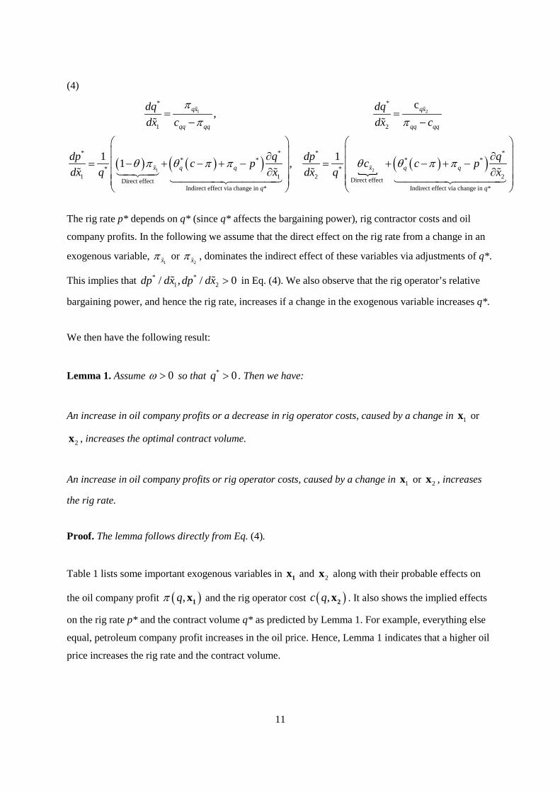
(4)
( ) ( )( )
( )( )
1 2
1 2
* *
1 2
* * * ** * * *
* *1 1 2 Direct effectDirect effect
Indirect effect via change in *
c,
1 11 ,
qx qx
qq qq qq qq
x q q x q q
q
dq dqdx c dx c
dp q dp qc p c c pdx q x dx q
ππ π
q π q π π q q π π
= =− −
∂ ∂
= − + − + − = + − + − ∂ ∂
))( ))))))))( 2
Indirect effect via change in *q
x
))))))))(
The rig rate p* depends on q* (since q* affects the bargaining power), rig contractor costs and oil
company profits. In the following we assume that the direct effect on the rig rate from a change in an
exogenous variable, 1x
π or 2xπ , dominates the indirect effect of these variables via adjustments of q*.
This implies that * *1 2/ , / 0dp dx dp dx > in Eq. (4). We also observe that the rig operator’s relative
bargaining power, and hence the rig rate, increases if a change in the exogenous variable increases q*.
We then have the following result:
Lemma 1. Assume 0ω > so that * 0q > . Then we have:
An increase in oil company profits or a decrease in rig operator costs, caused by a change in 1x or
2x , increases the optimal contract volume.
An increase in oil company profits or rig operator costs, caused by a change in 1x or 2x , increases
the rig rate.
Proof. The lemma follows directly from Eq. (4).
Table 1 lists some important exogenous variables in 1x and 2x along with their probable effects on
the oil company profit ( ),qπ 1x and the rig operator cost ( ),c q 2x . It also shows the implied effects
on the rig rate p* and the contract volume q* as predicted by Lemma 1. For example, everything else
equal, petroleum company profit increases in the oil price. Hence, Lemma 1 indicates that a higher oil
price increases the rig rate and the contract volume.

12
Table 1: Hypothesized direct effects of exogenous variables in the analytical model Variable Oil company profit Rig contractor
cost Rig rate Contract
volume Oil price Positive Positive Positive Remaining resource Positive Positive Positive Capital cost (real interest rate) Negative Positive Ambiguous Negative Labor cost (real wage) Negative Positive Ambiguous Negative Operation complexity Positive Positive Negative Oil company favorable regulation Positive Positive Positive Note: “Oil company favorable regulation” may e.g. include tax exemptions and lax environmental regulation.
Some entries in Table 1 warrant attention. First, several variables affect costs and benefits of the
agreement after the contract is signed (e.g., oil price and real interest rate). Thus, it is rather the
expected future values of these variables that matter. Second, some rig operations are more demanding
than others, e.g. because of deep water or harsh climate. This typically increases the rig operation cost,
but it seems unreasonable to expect it to induce shorter contract length for a given operation. On the
other hand, higher costs due to operational complexity imply that fewer projects are developed as
profits net of rig costs decrease.
The econometric model features rig and capacity utilization rates as its two endogenous variables. The
capacity utilization rate is the number of hired rig days divided by the number of available rig days.
For a given capacity q , capacity utilization is then equal to /q q in the theory model. We therefore
expect the theory model’s predictions regarding q to apply to the capacity utilization variable
(CAPUT) in the econometric model.
3. Data, aggregation and modelling framework Our point of departure is micro data, with floaters as the observational unit. We have to our disposition
540 observations of new contracts signed for the Norwegian continental shelf within a time interval
spanning the period from the start of the 1990’s to the end of 2013. Table A1 in Appendix A shows
the number of observations and the number of observational units behind the means in every period.
Note that in some periods the number of observational units is smaller than the number of
observations. The reason is that some observational units are represented by more than one
observation. The data have been obtained from the shipbroking company Clarksons Platou Offshore,
and include information about the daily rig rate for each contract. These rates are in current US$ and
we have deflated them by a producer price index to obtain rig rates in constant prices.9 The data also
9 We use the producer price index for “Industrial commodities less fuels” from http://www.bls.gov/data/home.htm. The base year is 2010.

13
include the fixture date, i.e., the date when the contract is signed, as well as the starting and end dates
for each contract. Thus, for every contract we can derive both the contract length and the lead time,
i.e., the number of days from the fixture date to the start date.10 The data also include rig-specific
information such as the year of construction, maximal drilling depth, and rig classification, see Table
2.11
Table 2. Overview of time series variables used for the reference model Variable Description Type of underly-
ing variable Source Denomination
rigrate Mean of log rig rates in constant prices
Varies across ob-servational unit and time
Clarksons Platou Offshore
USD (2010) per day
OILPRICE Oil price at constant prices
Time series from the outset
EIA US $ per barrel in fixed 2010-prices
CAPUT Capacity utilization Time series from the outset
Clarksons Platou Offshore
0<=CAPUT<=1
remres Log of remaining reserves
Time series from the outset
Norwegian Petrole-um Directorate
REMRES measured in Million standard cubic meter o. e.
RIR Real interest rate Time series from the outset
OECD Economic outlook
Annual rate in %
LEADTIME Mean of lead times Varies across ob-servational unit and time
Clarksons Platou Offshore
No. of days
depth Mean of log maxi-mal drilling depths
Time invariant characteristic
Clarksons Platou Offshore
DEPTH measured in feet
SHARE4a Share of rig type 4 Time invariant characteristic
Clarksons Platou Offshore
0<=SHARE4<=1
SHARE5a Share of rig type 5 Time invariant characteristic
Clarksons Platou Offshore
0<=SHARE5<=1
SEAS2 Seasonal dummy for the second quar-ter
Time series from the outset
T1 Step dummy Time series from the outset
1 until and includ-ing 1995q3, there-after 0
aSHARE4 and SHARE5 denote the share of contracts signed within a given quarter applying to rigs belonging to classes ‘SEMI 2. GEN’ and ‘SEMI 3. GEN’, respectively. See http://petrowiki.org/History_of_offshore_drilling_units for infor-mation about rig class specifications.
In our estimations (and forecasts) we implicitly consider the NCS as a separate market for floaters.
One motivation for this is that the number of rigs operating on the NCS is, at least in the short run,
10 The contract length, CONLENGTH, has been included in the empirical analysis, but is not included in the reference model . However, it is included in one of the alternative models in Appendix B. 11 There are three main rig types operating on the NCS: Jack-ups, semisubmersibles (of different generations), and drillships. The two latter categories are floaters. On the NCS, jack-ups rarely operate on water depths exceeding 130 meters. Semi-submersible rigs are moored to the sea floor and obtain buoyancy from ballasted pontoons located below the ocean surface. Drillships are specialized ships with drilling equipment. They are expensive but very mobile. The choice of rig type depends on the characteristics of the particular drilling operation. For more information, see e.g. Kaiser and Snyder (2013, Chap. 1.2).

14
little responsive to rig demand. Moving rigs over long distances is costly, especially for
semisubmersibles.12 Further, strict Norwegian regulations may impede rig relocation from e.g. the UK
Continental Shelf to the NCS, due to additional costs related to e.g. upgrading of living quarters,
lifting mechanisms, lighting and noise (Ministry of Petroleum and Energy, 2012). In the longer run,
however, the Norwegian rig market is likely to be somewhat influenced by other rig markets,
especially in the North Atlantic area. Moreover, from the data provided by Clarksons Platou Offshore
we have employed a variable for the capacity utilisation for floaters in the whole North Atlantic area.
Thus, our capacity utilization measure should be considered as a proxy for the capacity utilization on
the NCS. The utilization rate, which is then equal for all observations from the same time period,
shows considerable variation over the sample period (see Figure 2).
For the oil price we use the monthly Brent Blend price taken from the EIA (see Figure 2).13 These
prices are deflated by the same price index as used for the rig rates. We assume that oil companies’
price expectations are adaptive, meaning that their price expectations are continually updated based on
current and previous prices (see e.g., Farzin, 2001, Nguyen and Nabney, 2010, Aune et al., 2010, and
Osmundsen et al., 2015). Thus, we construct smoothed oil prices that are weighted averages of current
and historic prices. The smoothed oil price in period s (SOILPRICEs) is then assumed to follow a
Koyck lag structure, see Koyck (1954):
0( ) (1 ) ,
T js s j
jSOILPRICE OILPRICEα α α −
== −∑
where OILPRICEs is the real price of oil in period s.14
Annual time series for remaining reserves (REMRES) refer to petroleum resources that are expected to
be profitable to extract given current and expected economic conditions, and where plans for
development and operation of the petroleum deposits are either approved or submitted to the
12 According to the Ministry of Petroleum and Energy (2012), semisubmersibles accounted for 22 out of 23 floaters operating on the NCS by late December 2011 – the last one being a drillship. 13 http://www.eia.gov/dnav/pet/pet_pri_spt_s1_m.htm. For the period before 1987 we employ a monthly time series for the Brent Blend oil price provided by the Central Bank of Norway. 14 In principle, the sum should include price levels even longer back than T periods. However, we use T=47, which means that we use a filter spanning 12 years. Note that when T goes to infinity the sum of the weights equals 1 for all feasible values of α. As will be seen later, in the empirical part of the paper, our estimate of α implies that the estimate of the sum
0 (1 ) jTjα α= −∑ is very close to unity. We have therefore not modified the weights such that the sum of the estimated
weights is exactly equal to unity. This has no implications from a practical point of view.

15
government. The time series for this variable have been obtained from the Norwegian Petroleum
Directorate.15
From these data we construct quarterly time series by aggregation. The first period is 1991q4 and the
last period is 2013q4. The same observational unit is not observed in each quarter and it is also
common that one has more than one observation for an observational unit in some time periods. The
number of micro observations on which the quarterly observations are based varies from 1 to 24. For a
single quarter, i.e. 2008q4, there are no observations. Thus our time series contain one missing
observation. Our subsequent empirical analysis is based on these aggregate data together with
variables that are time series from the outset, such as the oil price.
Our micro dataset contains three variables that vary both across observational units and over time.
This is the rig rate in constant prices (RIGRATE), the length of the contract (CONLENGTH) and the
lead time associated with the contract (LEADTIME). For the rig rate we log-transform the data and
obtain the variable rigrate = log(RIGRATE). The variables rigrate, CONLENGTH and LEADTIME
are aggregated in the same manner, and below we show how the aggregation is carried out for rigrate.
Let ( )iit srigrate denote the t’th observation on the log of rig rates for rig i in period s. Let I(s) denote a
set consisting of the rigs present in period s. Let ti(s) take on the values 1i(s) to Ni(s). The un-weighted
mean of the values from period s is then given by
( )
( )( ) ( ) 1 ( )
( )
1 .( )
i
ii i
N s
s it si I s t s s
ii I s
rigrate rigrateN s ∈ =
∈
= ∑ ∑∑
The micro data set we apply contains several rig specific characteristics, i.e. variables that are time
invariant and only vary across different observational units. The different characteristics are indicated
in Table 2. One of these variables is the maximal drilling depth, DEPTH. As for the rig rates, we
consider the log-transformed variable, depth=log(DEPTH). The corresponding aggregate variable is
defined as
15 Estimates for remaining resources are retrieved from yearly publications over the period 1990 to 2014, named “Facts 1990”,…,”Facts 2014”, see http://www.npd.no/en/Publications/Facts/. The variable REMRES and the two companion variables POT and REMREC (See Table B3 in Appendix B) are all annual variables from the outset. They have been converted to quarterly time series in a technical way by using the convert option in TSP 5.0, cf. Hall and Cummins (2005, pp. 99-101).
16
( )
( )
1 ( )( )
s i ii I s
ii I s
depth N s depthN s ∈
∈
= ∑∑
Time series for the other time invariant variables are obtained in a similar manner.16
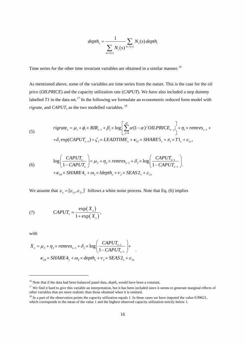
As mentioned above, some of the variables are time series from the outset. This is the case for the oil
price (OILPRICE) and the capacity utilization rate (CAPUT). We have also included a step dummy
labelled T1 in the data set.17 In the following we formulate an econometric reduced form model with
rigrates and CAPUTs as the two modelled variables. 18
(5)
47
1 1 1 1 1 10
1 1 1 15 1 1
log (1 )
exp( ) 5 1 ,
js s s j s
j
s s s s s
rigrate RIR OILPRICE remres
CAPUT LEADTIME SHARE T
m φ β α α η
δ ζ κ π e
− − −=
−
= + × + × − + × +
+ + × + × + × +
∑
(6) 1
2 2 1 21
24 2 2 2
log log1 1
4 2
s ss
s s
s s s s
CAPUT CAPUTremresCAPUT CAPUT
SHARE ldepth SEAS
m η δ
κ ω ν e
−−
−
= + × + × − −
+ × + × + × +
.
We assume that /1 2[ , ]s s se e e= follows a white noise process. Note that Eq. (6) implies
(7) ( )( )
exp1 exp
ss
s
XCAPUT
X=
+,
with
12 2 1 2
1
24 2 2 2
log1
4 2
ss s
s
s s s s
CAPUTX remresCAPUT
SHARE depth SEAS
m η δ
κ ω ν e
−−
−
= + × + × + −
× + × + × +
.
16 Note that if the data had been balanced panel data, depths would have been a constant. 17 We find it hard to give this variable an interpretation, but it has been included since it seems to generate marginal effects of other variables that are more realistic than those obtained when it is omitted. 18 In a part of the observation points the capacity utilization equals 1. In these cases we have imputed the value 0.99621, which corresponds to the mean of the value 1 and the highest observed capacity utilization strictly below 1.

17
Eq. (7) will be utilized later for forecasting purposes. We observe that the capacity utilization rate is
included in the rig rate equation, whereas the rig rate is not included in the equation for the capacity
utilization. This is consistent with the theoretical model, and is also consistent with our estimation of
all the alternative models, but one.
4. Estimation results
Reference model
The non-linear multivariate regression estimates of the reference model are provided in Table 3
below.19 Most of the parameter estimates in Table 3 are significant at the five percent level. The log of
the smoothed oil price only enters positively in the reduced form equation of the (log) rig rate with a
parameter estimate of 0.78, cf. the estimate of 1β . The estimate of the smoothing parameter, α, is 0.11.
This parameter weighs the importance of oil prices from different points of time. The estimate on 0.11
suggests that the expectations about future oil prices are updated quite fast to new oil price
observations. For example, the oil price three years ago weighs roughly one quarter of the present oil
price in the Koyck lag specification. We observe that the oil price only enters the rig rate equation.
Also the lagged real interest rate impacts the rig rate positively, cf. the estimate of φ1 in Table 3. A one
percentage point increase in the lagged real interest rate leads to a 0.078 increase in the log rig rate. In
the theory model we found that the real interest rate has an ambiguous effect on the rig rate (cf. Table
1). The reason is that the real interest rate increases the capital cost of oil companies, making them less
willing to pay for rigs, and increases the rig contractors’ capital costs and hence the cost of supplying
rigs. The positive estimate suggests that the rig contractor capital cost effect dominates in the period
1990-2014 in the NCS.
The lagged (antilog transformed) capacity utilization rate, i.e., ( )1exp sCAPUT − is yet another
variable that has a positive impact on the rig rate, cf. the estimate of δ1.20 This is as expected, because
higher capacity utilization increases both the bargaining power of the rig contractors and the cost of
supplying rigs (e.g., because of maintenance requirements). The same is true for the lagged lead time
variable, cf. the estimate of ζ1. We observe that a longer lead time suggests more pressure in the rig
market, and thus has similar effects on the rig rate as capacity utilization. 19 All the numerical calculations have been carried out using TSP 5.0, cf. Hall and Cummins (2005). 20 The reason for using the antilog transformation is that we a priori believe that the effect of an increase in the capacity utilization is stronger the higher the capacity utilization is.
18
We also find a significant positive effect of the lagged stock of remaining petroleum reserves (log-
transformed), cf. the estimate of the parameter η1. Intuitively, more available resources imply larger
profit potential for the oil companies, and hence increased rig demand. Finally a rig classification
variable and a step dummy are also present in the reduced form equation of the (log) rig rate, cf. the
estimates of the two parameters κ15 and π1. This reflects that rig characteristics differ across rigs, e.g.
with respect to rental costs and services the rig can supply.
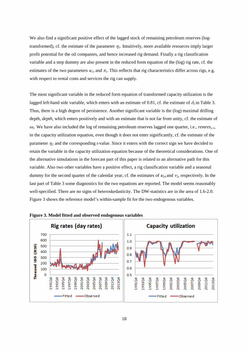
The most significant variable in the reduced form equation of transformed capacity utilization is the
lagged left-hand side variable, which enters with an estimate of 0.81, cf. the estimate of δ2 in Table 3.
Thus, there is a high degree of persistence. Another significant variable is the (log) maximal drilling
depth, depth, which enters positively and with an estimate that is not far from unity, cf. the estimate of
ω2. We have also included the log of remaining petroleum reserves lagged one quarter, i.e., remress-1,
in the capacity utilization equation, even though it does not enter significantly, cf. the estimate of the
parameter η2 and the corresponding t-value. Since it enters with the correct sign we have decided to
retain the variable in the capacity utilization equation because of the theoretical considerations. One of
the alternative simulations in the forecast part of this paper is related to an alternative path for this
variable. Also two other variables have a positive effect, a rig classification variable and a seasonal
dummy for the second quarter of the calendar year, cf. the estimates of κ24 and ν2, respectively. In the
last part of Table 3 some diagnostics for the two equations are reported. The model seems reasonably
well-specified. There are no signs of heteroskedasticity. The DW-statistics are in the area of 1.6-2.0.
Figure 3 shows the reference model’s within-sample fit for the two endogenous variables.
Figure 3. Model fitted and observed endogenous variables

19
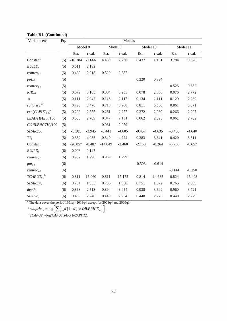
In Appendix B we report results for some other model specifications obtained by extending or
modifying the reference model with respect to exogenous variables used as regressors. Altogether
there are 11 such models. Model 6, which features a dummy variable for the petroleum tax relief in
2005, is of particular interest, suggesting that the Norwegian government policy to spur activity on the
NCS has worked as intended.
Table 3. Non-linear multivariate regression estimates Parameter Related variable etc. Estimate t-value Rig rate Eq. (5)
1m Constant 4.850 2.701
1φ remress-1 0.469 2.194
1η RIRs-1 0.079 3.009
α Smoothing parameter 0.110 2.135
1β soilpricesa 0.780 9.270
1δ exp(CAPUTs-1) 0.235 2.013
1ς LEADTIMEs-1/100 0.061 2.897
15κ SHARE5s -0.416 -4.258
1π T1 0.336 3.762
Capacity utilization Eq. (6)
2m Constant -14.050 -2.460
2η remress-1 0.938 1.299
2δ log(CAPUTs-1/(1-CAPUTs-1)) 0.811 15.174
24κ SHARE4s 0.736 1.950
2ω sdepth 0.894 3.456
2υ SEAS2s 0.441 2.257
Diagnostics: Number of observations 87
Sample period 1991q4-2013q4b
R2 Eq. (5) 0.836
DW Eq. (5) 1.808
LM-test for heteroskedasticity (p-value) Eq. (5) 0.183
R2 Eq. (6) 0.785
DW Eq. (6) 1.646
LM-test for heteroskedasticity (p-value) Eq. (6) 0.183
a ( )47
0ˆ ˆlog 1 j
s s jjsoilprice OILPRICEα α −=
= − × ∑ . b The data cover the period 1991q4-2013q4 except for 2008q4 and 2009q1.
20
5. Forecasts and forecast uncertainty of the rig rate and the ca-pacity utilization rate
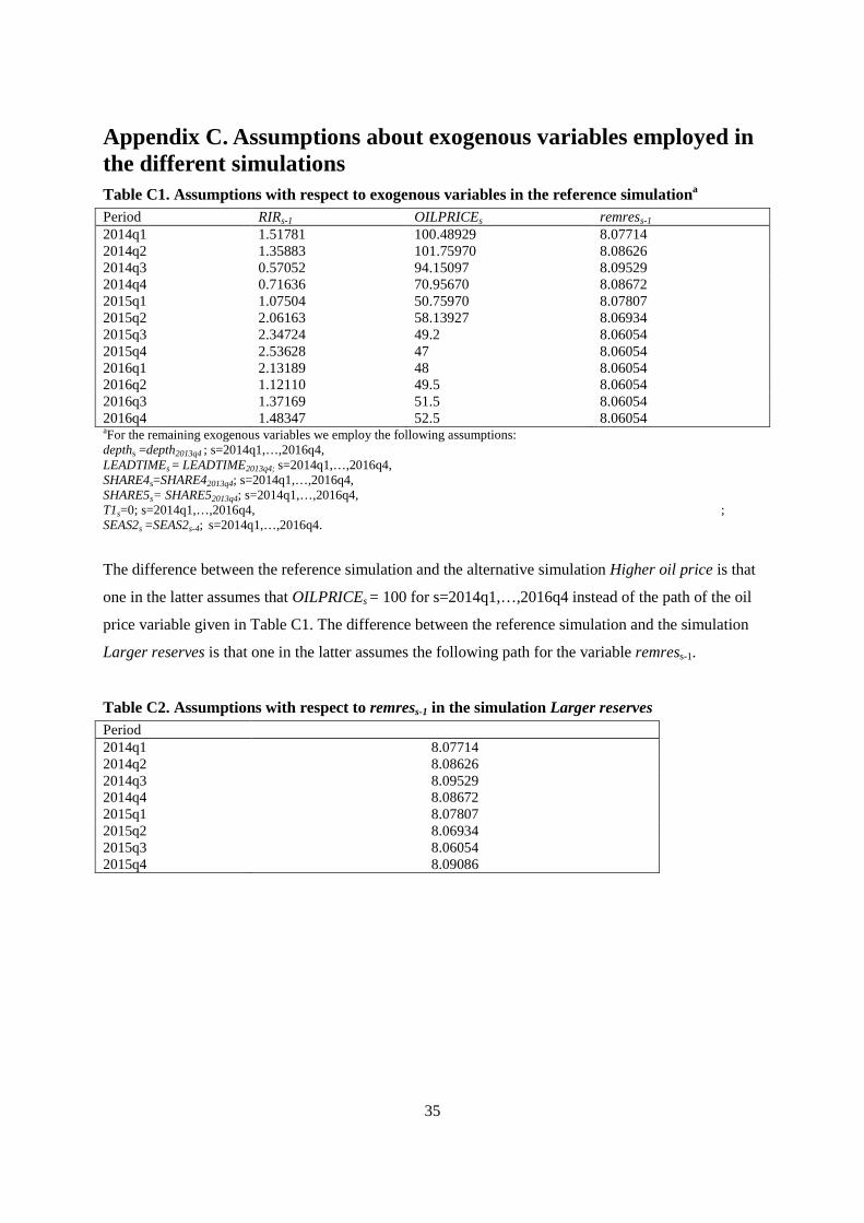
In this part of the paper we present conditional forecasts for the period 2014q1-2016q4 using the
reference model. We distinguish between a reference simulation and two alternative simulations,
which we label, respectively, “Higher oil price” and “Larger reserves”. Appendix C contains
information on what have been assumed for the exogenous variables for the simulation period 2014q1-
2016q4. For all the three simulations we report point forecasts, whereas we for the reference
simulation also consider forecast uncertainty stemming from the errors. In Appendix D we give an
account of how the forecast uncertainty is calculated by a bootstrap approach.21 Our point forecasts are
also based on results from the bootstrap procedure. We employ the mean forecasts across the
replications. An argument for this is that the econometric model is formulated in transformed
variables, whereas we focus on forecasting the untransformed variables.
In Figure 4 we show the point forecasts of RIGRATE and CAPUT obtained in the reference simulation
together with the implied forecast uncertainty. The assumptions with respect to the exogenous
variables used in conjunction with the reference simulation are given in Table C1 in Appendix C and
the involved parameter estimates are those reported in Table 3. According to the reference simulation,
both the rig rate, RIGRATE, and the capacity utilization, CAPUT, are predicted to fall from the
beginning of 2014 to the end of 2016. The rig rate is predicted to fall by 28 percent whereas the
capacity utilization is predicted to decrease by 14 percentage points (from 2013q4 to 2016q4). A major
factor behind this drop in the rig rate is the substantial fall in the oil price (in constant prices), even if
this fall is somewhat dampened since we use a smoothed oil price as an explanatory variable. As seen
from the second column of Table C1 in Appendix C, the oil price in fixed prices is more than halved
from the start of 2014 to the end of 2015 and is assumed to increase only moderately during 2016. The
oil price observations in the period 2014q1 to 2015q2 correspond to observed values, while for the
remaining period we have made assumptions in the light of the development of future prices. The
estimated capacity utilization equation is dominated by an autoregressive slope coefficient somewhat
below unity. This feature contributes to a reduction in the capacity utilization during the forecast
period, which gives negative impulses to the rig rate.
21 For bootstrap methods for time series see Kreiss and Lahiri (2012).

21
Figure 4. Forecasts of rig rates and capacity utilization in the reference simulation, including 50% forecast intervals. See Table C3 and Table C4 in Appendix C for the basis of the figures
In Figure 4 we report 50% forecast intervals for the values of the two endogenous variables, i.e.,
RIGRATEs and CAPUTs in the period 2014q1-2016q4.22 The forecasts intervals account for
uncertainty stemming from the errors of the two equations.23 How the forecast intervals have been
calculated is outlined in Appendix D. The forecast intervals for the rig rate are rather wide. In 2016q4,
the last quarter that we consider, the calculated forecast interval of the rig rate starts at 282 thousand
USD per day and ends at 373 thousand. The corresponding values for the capacity utilization are 0.84
and 0.97. If one looks at the ratios between the length of the forecast interval and the point forecast,
they increase moderately for the rig rate over time, whereas there is a larger increase for the capacity
utilization rate. The reason for this feature is that there is no lagged rig rate involved in the reference
model, and that the estimated slope parameter of the lagged transformed capacity utilization variable
in the rig rate equation, i.e., exp(CAPUTs-1), is relatively moderate in size, dampening the contribution
of lagged errors in the capacity utilization equation to the forecast errors of the rig rate equation.
In Figure 5 we show the point forecasts based on the reference models together with the forecasts
under the two alternative simulations, Higher oil price and Larger reserves. In the Higher oil price
simulation we assume another, partly counterfactual, path of the oil price by setting it to 100 USD per
22 Granger (1996) suggested that a 50 percent forecast interval tends to be more interesting from a practical point of view compared to a 90 percent interval since the latter commonly yields a rather wide interval. 23 Note that the forecast intervals are asymmetric around the point forecasts. This feature follows from how the intervals are calculated. As explained in Appendix D, the lower and upper levels of the intervals correspond to the first and third quartiles in the distributions of replicated forecasts. Since the distributions are skew the mean of the distributions deviates from median value.

22
barrel (in constant prices) for the entire period 2014q1-2016q4, i.e., close to the price at the beginning
of the forecast period. Accordingly, the rig rate shows only a slight reduction from 2014q1-2016q4. As
we noted earlier, the capacity utilization does not depend on the oil price, which implies that the
capacity utilization path is the same for the reference simulation and the higher oil price simulation. In
the Larger reserves simulation we are looking at the implications on the NCS rig market following
opening for petroleum activity in the Barents Sea and areas around Jan Mayen. The associated
increase in petroleum reserves is 12.3 percent, relative to the reference simulation. However, since this
variable enters with a lag, we see from tables C1 and C2 in Appendix C that it is not until 2015q4 that
the Larger reserves deviates from the reference simulation. The petroleum reserve variable, remres,
impacts both the rig rate and the capacity utilization variables positively. This is the reason why the
reduction in the rig rate from 2014q1 to 2016q4 is less than in the reference simulation. However, the
large decrease in the petroleum price also dominates in this case, giving a reduction in the rig rate
from 2013q4 to 2016q4 of 23 percent. The capacity utilization decreases less in this simulation than in
the reference simulation since an increase in the petroleum reserves gives positive impulse to the
capacity utilization.
Figure 5. Forecasts of rig rates and capacity utilization in the reference simulation and in the Higher oil price and Larger reserves simulations. See Table C3 in Appendix C for the basis of the graphs

23
6. Concluding remarks In this paper we first presented a simple theoretical model to sharpen our understanding of rig markets
and help identify the most important drivers for rig rate formation. Then we estimated their effects in
the NCS rig market for floaters, using a reduced form two-equation time series econometric model for
rig rates and a proxy for capacity utilization over the period 1991q4 to 2013q4. Last, we presented
point and interval forecasts for rig rates on the NCS and capacity utilization in the North Atlantic area
in a reference simulation and point forecasts for two alternative simulations. The first alternative
simulation featured a relatively high oil price (constant at 2014q1 level), and the second involved
opening for petroleum activity in new areas.
The results from our econometric analysis of rig rate formation and utilization rates at the NCS are
roughly in line with the hypothesized effects from the theoretical model (compare Table 1 with Table
3). Based on the assumption of adaptive oil price expectations according to the Koyck lag structure,
we found that expectations about future oil prices are updated quite fast to new oil price observations.
In particular, higher oil prices stimulate petroleum development projects. The rig rates then increase
because rig operators capture a share of the profitability from petroleum activity, and because higher
rig demand induces higher capacity utilization, which again increases the rig operators’ relative
bargaining strength. On the other hand, we were not able to find a significant positive effect on
capacity utilization from higher oil prices. Possible explanations are the highly persistent nature of
capacity utilization, and that the endogenous capacity variable CAPUT is a proxy variable, since it
covers a wider area than the NCS. Because CAPUT shows very strong persistence, this is not very
problematic with respect to forecasting, given the relatively short forecasting horizon we consider
(three years). We found some evidence that increased remaining petroleum reserves stimulate demand
for rigs, and hence rig rates and capacity utilization. Lastly, we found significant effects of two rig
classification variables and maximum drilling depth. These are again roughly in line with the theory.
The oil price is roughly halved from 2013q4 to 2016q4 in our reference simulation, causing a
substantial decline in rig rates and capacity utilization over the forecasting horizon. The rig rate is
predicted to fall by 28 percent, whereas the capacity utilization is predicted to decrease by 14
percentage points (from 2013q4 to 2016q4). In contrast, the rig rate remains roughly at the same level
in the high oil price simulation, where the oil price is constant at the 2014q1 level. Capacity utilization
declines in this simulation too, however. In the second alternative simulation we analyzed effects on
the NCS rig market following opening for petroleum activity in the Barents Sea and around Jan
Mayen. As expected, this induced higher rig rates and capacity utilization, as compared with the

24
reference simulation. Both rig rates and capacity utilization decline over time in this simulation too,
because the sharp decline in the oil price dominates the effect from increased petroleum reserves.
The empirical model in this paper applies to the NCS. Nevertheless, it seems reasonable to expect that
many of the variables recognized in this study will also be important constituents of rig rates in other
geographical areas where off-shore drilling is applied, in particular as deepwater reserves become
more important.

25
References Aune, F.R., K. Mohn, P. Osmundsen and K.E. Rosendahl (2010): Financial market pressure, tacit collusion and oil price formation. Energy Economics 32 (2), 389–398. Boyce, J. R. and L. Nøstbakken (2011): Exploration and development of U.S. oil and gas fields, 1955–2002. Journal of Economic Dynamics and Control 35 (6), 891–908. BP (2015): BP Statistical Review of World Energy June 2015, BP. http://www.bp.com/statisticalreview Corts, K.S. (2008): Stacking the deck: idling and reactivation of capacity in offshore drilling. Journal of Economic Management and Strategy 17 (2), 271–294. EIA (2011): Annual Energy Review 2010. US Energy Information Administration, October 2011. Hall, B.H. and C. Cummins (2005): TSP 5.0 Reference Manual. TSP international. Farzin, Y.H. (2001): The impact of oil prices on additions to US proven reserves. Resource and Energy Economics 23 (3), 271–291. Granger, C.W.J. (1996): Can We Improve the Perceived Quality of Economic Forecasts? Journal of Applied Econometrics, 11 (5), 455–473. Iledare, O.O. (1995): Simulating the effect of economic and policy incentives on natural gas drilling and gross reserve additions. Resource and Energy Economics 17 (3), 261–279. Kaiser, M.J. and B.F. Snyder (2013): The Offshore Drilling Industry and Rig Construction in the Gulf of Mexico. Springer Science & Business Media. Kellogg, R. (2011): Learning by drilling: interfirm learning and relationship persistence in the Texas oilpatch. Quarterly Journal of Economics 126 (4), 1961–2004. Kemp, A. and S. Kasim (2003): An Econometric Model of Oil and Gas Exploration Development and Production in the UK Continental Shelf: A Systems Approach. The Energy Journal 24 (2), 113–141. Koyck, L.M. (1954): Distributed Lags and Investment Analysis. North-Holland, Amsterdam. Kreiss, J.-P. and S.N. Lahiri (2012): Bootstrap Methods for Time Series. Chapter 1 in Rao, T.S., Rao, S.S. and C.R. Rao (Eds.): Handbook of Statistics. Volume 30. Time Series Analysis: Methods and Applications. North-Holland, Amsterdam, pp. 3–26. Lin, C. (2009): Estimating strategic interactions in petroleum exploration. Energy Economics 31 (4), 586–594. Ministry of Petroleum and Energy (2012): An industry for the future – Norway’s petroleum activities — Meld. St. 28 (2010–2011) Report to the Storting (white paper). Ministry of Petroleum and Energy, August 2012. Available at: https://www.regjeringen.no/en/dokumenter/meld.-st.-28-20102011/id649699/ Mohn, K. (2008): Efforts and efficiency in oil exploration: a vector error-correction approach. The Energy Journal 29 (4), 53–78.
26
Mohn, K. and P. Osmundsen (2008): Exploration economics in a regulated petroleum province: the case of the Norwegian continental shelf. Energy Economics 30 (2), 303–320. Nguyen, H.T. and I.T. Nabney (2010): Short-term electricity demand and gas price forecasts using wavelet transforms and adaptive models. Energy 35 (9), 3674–3685. Norwegian Petroleum Directorate (2014): Facts 2014. Norwegian Petroleum Directorate, 2014. Available at: http://www.npd.no/en/Publications/Facts/ Osmundsen, P., Roll, K. H. and R. Tveterås (2010a): Exploration drilling productivity at the Norwegian shelf. Journal of Petroleum Science and Engineering 73 (1-2), 122–128. Osmundsen, P., Roll, K. H. and R. Tveterås (2010b): Drilling speed - the relevance of experience. Energy Economics 34 (3), 786–794. Osmundsen, P., K. E. Rosendahl and T. Skjerpen (2015): Understanding rig rate formation in the Gulf of Mexico. Energy Economics 49, 430–439. Ringlund, G. B., K. E. Rosendahl and T. Skjerpen (2008): Does oilrig activity react to oil price changes? An empirical investigation. Energy Economics 30 (2), 371–396. Seber, G.A.F. and C.J. Wild (1989): Nonlinear regression. John Wiley & Son. Watson, J. (2002): Strategy: an introduction to game theory. W. W. Norton & Company.

27
Appendix A. Information related to the micro data source Table A1. Number of micro observations behind the aggregate data in each time period Period No. of
micro obs.
No. of rigs N(s)
Period No. of micro obs.
No. of rigs
Period No. of micro obs.
No. of rigs
1990q4 2 2 1999q1 5 5 2007q2 4 2 1991q1 1 1 1999q2 11 7 2007q3 9 3 1991q2 2 2 1999q3 10 8 2007q4 3
3 1991q3 4 4 1999q4 6 6 2008q1 8 4 1991q4 10 10 2000q1 8 6 2008q2 6 4 1992q1 4 4 2000q2 15 8 2008q3 3 1 1992q2 4 4 2000q3 5 4 2008q4 0 0 1992q3 6 5 2000q4 10 9 2009q1 4 3 1992q4 2 2 2001q1 8 6 2009q2 1 1 1993q1 4 4 2001q2 11 7 2009q3 3 3 1993q2 5 5 2001q3 10 6 2009q4 5 4 1993q3 6 6 2001q4 5 4 2010q1 2 2 1993q4 4 4 2002q1 2 2 2010q2 6 4 1994q1 2 2 2002q2 1 1 2010q3 3 3 1994q2 1 1 2002q3 5 5 2010q4 7 5 1994q3 6 5 2002q4 10 7 2011q1 3 3 1994q4 2 2 2003q1 9 6 2011q2 3 3 1995q1 2 1 2003q2 2 2 2011q3 7 6 1995q2 5 4 2003q3 2 2 2011q4 2 2 1995q3 5 4 2003q4 3 2 2012q1 5 5 1995q4 6 5 2004q1 16 8 2012q2 4 4 1996q1 6 6 2004q2 9 5 2012q3 3 3 1996q2 5 4 2004q3 2 2 2012q4 5 5 1996q3 6 5 2004q4 6 6 2013q1 1 1 1996q4 7 4 2005q1 24 6 2013q2 1 1 1997q1 11 10 2005q2 7 3 2013q3 3 3 1997q2 5 5 2005q3 15 7 2013q4 2 2 1997q3 5 4 2005q4 12 5 1997q4 7 4 2006q1 7 5 1998q1 7 5 2006q2 14 6 1998q2 5 5 2006q3 9 5 1998q3 5 3 2006q4 11 8 1998q4 6 6 2007Q1 9 6

28
Appendix B. Alternative econometric model structures In this appendix we show the estimation results from alternative model structures. Whereas estimates
of the unknown parameters are reported in Table B1, some diagnostics for the residuals are reported in
Table B2. The other models are obtained by extending or modifying the reference model in different
ways. An overview of additional variables involved when estimating these models is given in Table
B3. Altogether there are 11 additional models, and we label them Model 1-Model 11. In Model 1 we
allow the log of the smoothed oil price to enter also the capacity utilization equation. The significance
of the estimate turns out to be very low. In Model 2 we add the log of the rig rate lagged one quarter.
The estimate of the attached coefficient is, as expected, positive, but insignificant at the 5 percent
level. It seems that the estimates of the other parameters are qualitatively very equal to the ones
obtained for the reference model. In Model 3 we allow the log rig rate lagged one period to enter both
equations. The estimates of the two coefficients attached to this additional variable are positive, but
insignificant. Again the estimates of the other parameters are little influenced, as the coefficient
estimates are rather equal to those obtained for the reference model.
Models 4-6 are all concerned with policy changes. In each case the policy change is represented by a
step dummy. The step-dummies are zero before the policy changes are carried out and thereafter equal
to unity. All the policy changes are expected to have a positive effect on both the rig rate and the
capacity utilization. In Model 4 we add a variable, DUM1999, representing changes in the routines
related to allocation of licenses through the establishment of the so-called North Sea Awards (NSA)
scheme, which developed in 2003 into the Awards in Predefined Areas (APA) scheme. The aim was to
increase activity in mature areas. Both the estimate of the parameter attached to this variable in the rig
rate equation and the estimate attached to this variable in the capacity utilization equation are
insignificant at the 5 per cent significance level. The estimate of the parameter in the rig rate equation
is positive, whereas the estimate of the parameter in the capacity utilization equation is negative,
which is in contrast to what was expected. Next, in Model 5 we add a step-dummy, DUM2000, related
to prequalifying of operators and licensees. This aimed to make it simpler for a new company to
secure access to acreage, either through license awards or through buying/swopping license interests.
The estimates of two parameters attached to this policy variable are negative and insignificant. The
third policy variable, DUM2005, is allowed to enter in Model 6. This variable represents a petroleum
tax relief, giving companies with a tax loss the right to annual refunding of the tax value (78 per cent)
of exploration costs. Alternatively, such losses can be carried forward as a tax deduction in later years
with an interest supplement. The variable enters with the expected sign in both equations, and in the
rig rate equation the estimate is close to be being significant at the 5 per cent level.

29
In Model 7 the lagged real interest rate, RIRs-1, is also allowed to enter the capacity utilization
equation. A negative and insignificant estimate is obtained. In Model 8 we consider the effect of the
mean building year, BUILD. This variable picks up technological improvement over time. It enters
positively in both equations, but only significantly so in the rig rate equation. The estimates of the
other parameters are, at least qualitatively, rather equal to the estimates obtained for the reference
model.
In Model 9 the contract length, CONLENGTHs, is added to the rig rate equation. A positive and
marginal significant estimated effect is obtained. From a qualitative point of view the model share the
properties of the reference model, but there are some numerical differences. The point estimates of the
adjustment parameter and the parameter attached to LEADTIMEs-1 are, e.g., somewhat larger in Model
9 than in the reference model.
Whereas Model1-Model9 all are extension of the reference model, Model 10 and Model 11 are
modifications of the reference model. In Model 10 the variable for remaining resources, remress-1, is
replaced by a variable representing the log of total production potential minus accumulated production
lagged one quarter, which we label pott-1 and in Model 11 by a variable for the log of remaining
resources lagged one quarter, which we have dubbed remrecs-1. None of these variables enter
significantly in any of the equations. All the four t-values are well below unity in absolute value.

30
Table B1. Non-linear multivariate regression estimates of additional modelsa
Variable etc.
Eq
Models
Reference model Model 1 Model 2 Model 3
Est. t-val. Est. t-val. Est. t-val. Est. t-val.
Constant (5) 4.850 2.701 4.847 2.697 4.631 2.648 4.628 2.646
rigrates-1 (5) 0.101 1.108 0.101 1.114
remress-1 (5) 0.469 2.194 0.470 2.194 0.400 1.852 0.400 1.850
RIRs-1 (5) 0.079 3.009 0.079 3.008 0.072 2.723 0.073 2.724
α (5) 0.110 2.135 0.109 2.134 0.118 1.917 0.118 1.917
soilpricesb (5) 0.780 9.270 0.780 9.263 0.683 5.761 0.683 5.762
exp(CAPUTs-1) (5) 0.235 2.013 0.235 2.014 0.205 1.714 0.204 1.710
LEADTIMEs-1/100 (5) 0.061 2.897 0.061 2.898 0.059 2.769 0.059 2.769
SHARE5s (5) -0.416 -4.258 -0.416 -4.257 -0.423 -4.350 -0.423 -4.349
T1s (5) 0.336 3.762 0.336 3.758 0.311 3.440 0.310 3.439
Constant (6) -14.050 -2.460 -14.088 -2.458 -14.052 -2.461 -14.600 -2.530
rigrates-1 (6) 0.114 0.603
remress-1 (6) 0.938 1.299 0.942 1.301 0.936 1.296 0.861 1.177
α (6) 0.109 2.134
soilpricesb (6) -0.016 -0.078
TCAPUTs-1c (6) 0.811 15.174 0.813 14.319 0.811 15.177 0.799 14.024
SHARE4s (6) 0.736 1.950 0.740 1.944 0.734 1.943 0.711 1.879
depths (6) 0.894 3.456 0.902 3.281 0.896 3.463 0.870 3.320
SEAS2s (6) 0.441 2.257 0.441 2.259 0.441 2.255 0.428 2.185

31
Table B1. (Continued)
Variable etc.
Eq.
Models
Model 4 Model 5 Model 6 Model 7
Est. t-val. Est. t-val. Est. t-val. Est. t-val.
Constant (5) 4.173 1.894 4.843 2.911 7.210 3.212 4.858 2.704
DUM1999s (5) 0.150 1.409
DUM2000s (5) -0.094 -0.723
DUM2005s (5) 0.317 1.915
remress-1 (5) 0.521 2.056 0.477 2.375 0.308 1.288 0.469 2.189
RIRs-1 (5) 0.084 3.263 0.078 2.961 0.064 2.433 0.078 2.997
α (5) 0.072 1.504 0.146 1.945 0.090 1.382 0.109 2.135
soilpricesb (5) 0.766 7.681 0.814 8.327 0.550 3.739 0.780 9.269
exp(CAPUTs-1) (5) 0.325 2.436 0.183 1.304 0.132 1.035 0.234 2.006
LEADTIMEs-1/100
(5) 0.062 2.983 0.058 2.704 0.048 2.216 0.061 2.898
SHARE5s (5) -0.419 -4.346 -0.417 -4.291 -0.416 -4.339 -0.416 -4.257
T1s (5) 0.401 3.585 0.307 3.144 0.328 3.475 0.336 3.758
Constant (6) -16.859 -2.889 -15.333 -2.531 -13.248 -2.176 -12.956 -2.196
DUM1999s (6) -0.332 -1.752
DUM2000s (6) -0.120 -0.621
DUM2005s (6) 0.087 0.379
remress-1 (6) 1.219 1.679 1.058 1.416 0.869 1.171 0.849 1.160
RIRs-1 (6) -0.042 -0.709
TCAPUTs-1c (6) 0.813 15.477 0.813 15.223 0.800 12.950 0.801 14.482
SHARE4s (6) 0.747 2.015 0.739 1.962 0.719 1.902 0.722 1.915
depths (6) 0.991 3.792 0.944 3.509 0.863 3.147 0.864 3.306
SEAS2s (6) 0.445 2.324 0.440 2.258 0.436 2.228 0.434 2.224
32
Table B1. (Continued) Variable etc. Eq. Models
Model 8 Model 9 Model 10 Model 11
Est. t-val. Est. t-val. Est. t-val. Est. t-val.
Constant (5) -16.784 -1.666 4.459 2.730 6.437 1.131 3.784 0.526
BUILDs (5) 0.011 2.182
remress-1 (5) 0.460 2.218 0.529 2.687
pots-1 (5) 0.220 0.394
remrecs-1 (5) 0.525 0.682
RIRs-1 (5) 0.079 3.105 0.084 3.235 0.078 2.856 0.076 2.772
α (5) 0.111 2.042 0.148 2.117 0.134 2.111 0.129 2.239
soilpricesb (5) 0.723 8.476 0.718 8.968 0.811 5.560 0.861 5.071
exp(CAPUTs-1)c (5) 0.298 2.555 0.261 2.277 0.272 2.060 0.266 2.207
LEADTIMEs-1/100
(5) 0.056 2.709 0.047 2.131 0.062 2.825 0.061 2.782
CONLENGTHs/100
(5) 0.031 2.059
SHARE5s (5) -0.381 -3.945 -0.441 -4.605 -0.457 -4.635 -0.456 -4.640
T1s (5) 0.352 4.055 0.340 4.224 0.383 3.641 0.420 3.511
Constant (6) -20.057 -0.487 -14.049 -2.460 -2.150 -0.264 -5.756 -0.657
BUILDs (6) 0.003 0.147
remress-1 (6) 0.932 1.290 0.939 1.299
pots-1 (6) -0.508 -0.614
remrecs-1 (6) -0.144 -0.150
TCAPUTs-1b (6) 0.811 15.060 0.811 15.175 0.814 14.685 0.824 15.408
SHARE4s (6) 0.734 1.933 0.736 1.950 0.751 1.972 0.765 2.009
depths (6) 0.868 2.513 0.894 3.454 0.938 3.649 0.960 3.721
SEAS2s (6) 0.439 2.248 0.440 2.254 0.448 2.276 0.449 2.279 a The data cover the period 1991q4-2013q4 except for 2008q4 and 2009q1.
b ( )47
0ˆ ˆlog 1 j
s s jjsoilprice OILPRICEα α −=
= − × ∑ . c TCAPUTs =log(CAPUTs)-log(1-CAPUTs).

33
Table B2. Estimation diagnostics Model R2 DW LM-test for hetero-
skedasticitya
Rigrate Reference model 0.836 1.808 0.183 Model 1 0.836 1.808 0.183 Model 2 0.838 2.000 0.148 Model 3 0.838 2.001 0.148 Model 4 0.839 1.867 0.295 Model 5 0.837 1.804 0.165 Model 6 0.843 1.906 0.253 Model 7 0.836 1.808 0.184 Model 8 0.845 1.728 0.128 Model 9 0.843 1.794 0.239 Model 10 0.827 1.707 0.360 Model 11 0.827 1.723 0.332 log[CAPUT/(1-CAPUT)] Reference model 0.785 1.646 0.356 Model 1 0.785 1.647 0.361 Model 2 0.785 1.645 0.356 Model 3 0.786 1.638 0.292 Model 4 0.792 1.661 0.407 Model 5 0.786 1.639 0.374 Model 6 0.785 1.635 0.331 Model 7 0.786 1.630 0.355 Model 8 0.785 1.639 0.357 Model 9 0.785 1.646 0.356 Model 10 0.781 1.614 0.287 Model 11 0.781 1.618 0.321 a The figures reported in this column are significance probabilities. The null hypothesis is no heteroskedasticity.

34
Table B3. Additional variables involved for the models in Appendix B Variable Description Type of underlying
variable Source Denomination
CONLENGTH Mean of lead times Varies across ob-servational unit and time
Clarksons Platou Offshore
No. of days
BUILD Mean building year of rigs
Time invariant characteristic
Clarksons Platou Offshore
Years
pot Log of production potential less ac-cumulated produc-tion
Time series from the outset
Norwegian Petro-leum Directorate
Million standard cubic meter o. e.
remrec Log of remaining resources
Time series from the outset
Norwegian Petro-leum Directorate
Million standard cubic meter o. e.
DUM1999 Switch from 0 to 1 in 1999
Step dummy Norwegian Petro-leum Directorate
Binary variable
DUM2000 Switch from 0 to 1 in 2000
Step dummy Norwegian Petro-leum Directorate
Binary variable
DUM2005 Switch from 0 to 1 in 2005
Step dummy Norwegian Petro-leum Directorate
Binary variable
35
Appendix C. Assumptions about exogenous variables employed in the different simulations Table C1. Assumptions with respect to exogenous variables in the reference simulationa
Period RIRs-1 OILPRICEs remress-1 2014q1 1.51781 100.48929 8.07714 2014q2 1.35883 101.75970 8.08626 2014q3 0.57052 94.15097 8.09529 2014q4 0.71636 70.95670 8.08672 2015q1 1.07504 50.75970 8.07807 2015q2 2.06163 58.13927 8.06934 2015q3 2.34724 49.2 8.06054 2015q4 2.53628 47 8.06054 2016q1 2.13189 48 8.06054 2016q2 1.12110 49.5 8.06054 2016q3 1.37169 51.5 8.06054 2016q4 1.48347 52.5 8.06054 aFor the remaining exogenous variables we employ the following assumptions: depths =depth2013q4 ; s=2014q1,…,2016q4, LEADTIMEs = LEADTIME2013q4; s=2014q1,…,2016q4, SHARE4s=SHARE42013q4; s=2014q1,…,2016q4, SHARE5s= SHARE52013q4; s=2014q1,…,2016q4, T1s=0; s=2014q1,…,2016q4, ; SEAS2s =SEAS2s-4; s=2014q1,…,2016q4.
The difference between the reference simulation and the alternative simulation Higher oil price is that
one in the latter assumes that OILPRICEs = 100 for s=2014q1,…,2016q4 instead of the path of the oil
price variable given in Table C1. The difference between the reference simulation and the simulation
Larger reserves is that one in the latter assumes the following path for the variable remress-1.
Table C2. Assumptions with respect to remress-1 in the simulation Larger reserves Period 2014q1 8.07714 2014q2 8.08626 2014q3 8.09529 2014q4 8.08672 2015q1 8.07807 2015q2 8.06934 2015q3 8.06054 2015q4 8.09086
36
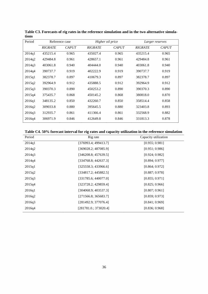
Table C3. Forecasts of rig rates in the reference simulation and in the two alternative simula-tions Period Reference case Higher oil price Larger reserves
RIGRATE CAPUT RIGRATE CAPUT RIGRATE CAPUT
2014q1 435215.4 0.965 435027.4 0.965 435215.4 0.965
2014q2 429484.8 0.961 428657.1 0.961 429484.8 0.961
2014q3 403061.8 0.940 404444.0 0.940 403061.8 0.940
2014q4 390737.7 0.919 402222.9 0.919 390737.7 0.919
2015q1 382378.7 0.897 410679.3 0.897 382378.7 0.897
2015q2 392964.9 0.912 435888.5 0.912 392964.9 0.912
2015q3 390370.3 0.890 450253.2 0.890 390370.3 0.890
2015q4 375435.7 0.868 450145.2 0.868 380818.0 0.870
2016q1 348135.2 0.850 432260.7 0.850 358514.4 0.858
2016q2 309033.8 0.880 395645.5 0.880 323403.8 0.893
2016q3 312935.7 0.861 411366.4 0.861 332568.9 0.882
2016q4 306971.9 0.846 412649.8 0.846 331813.3 0.878
Table C4. 50% forecast interval for rig rates and capacity utilization in the reference simulation Period Rig rate Capacity utilization
2014q1 [376993.4; 499413.7] [0.955; 0.981]
2014q2 [369028.2; 487085.9] [0.951; 0.986]
2014q3 [346208.8; 457639.5] [0.924; 0.982]
2014q4 [334768.8; 442637.3] [0.894; 0.977]
2015q1 [325558.3; 433966.6] [0.864; 0.972]
2015q2 [334817.2; 445882.5] [0.887; 0.978]
2015q3 [331785.6; 440077.0] [0.855; 0.971]
2015q4 [323728.2; 429859.4] [0.825; 0.966]
2016q1 [304068.9; 403537.3] [0.807; 0.961]
2016q2 [271566.8; 365683.7] [0.859; 0.973]
2016q3 [281492.9; 377076.4] [0.841; 0.969]
2016q4 [281781.0.; 373020.4] [0.836; 0.968]

37
Appendix D. Forecasting and forecasting uncertainty Let:
(8) ,s s s sy rigrate x CAPUT= = ,
Our model may then be specified as:
(9)
( ) ( ) ( )11 1 1 2 2
1
exp , , log log ,1 1
s ss s s ys s xs
s s
x xy x g Z h Mx x
δ l e δ l e−−
−
= + + = + + − −
where ( )1,sg Z l and ( )2,sh M l are terms that capture the effects of the exogenous variables. Let ^
denote a multiple regression estimate. Then residuals may be calculated as:
(10)
( ) ( ) ( )11 1 1 2 2
1
ˆ ˆ ˆ ˆˆ ˆexp , , log log ,1 1
s sys s s s xs s
s s
x xy x g Z h Mx x
e δ l e δ l−−
−
= − + = − + − −
Let S denote the number of observations in the estimation period. The 2Sx matrix with residuals is
given by:
(11)
1991 4 1991 4
2008 3 2008 3
2009 2 2009 2
2013 4 2013 4
ˆ ˆ
ˆ ˆˆ
ˆ ˆ
ˆ ˆ
y q x q
y q x qyx
y q x q
y q x q
e e
e ee
e e
e e
=
4 4
4 4
Consider (10) for the first 12 quarters after the last observation in the estimation sample. Then the
following 24 error terms are involved:
(12) 2014 1 2014 2 2016 4
2014 1 2014 2 2016 4
y q y q y qFyx
x q x q x q
e e ee
e e e
=
38
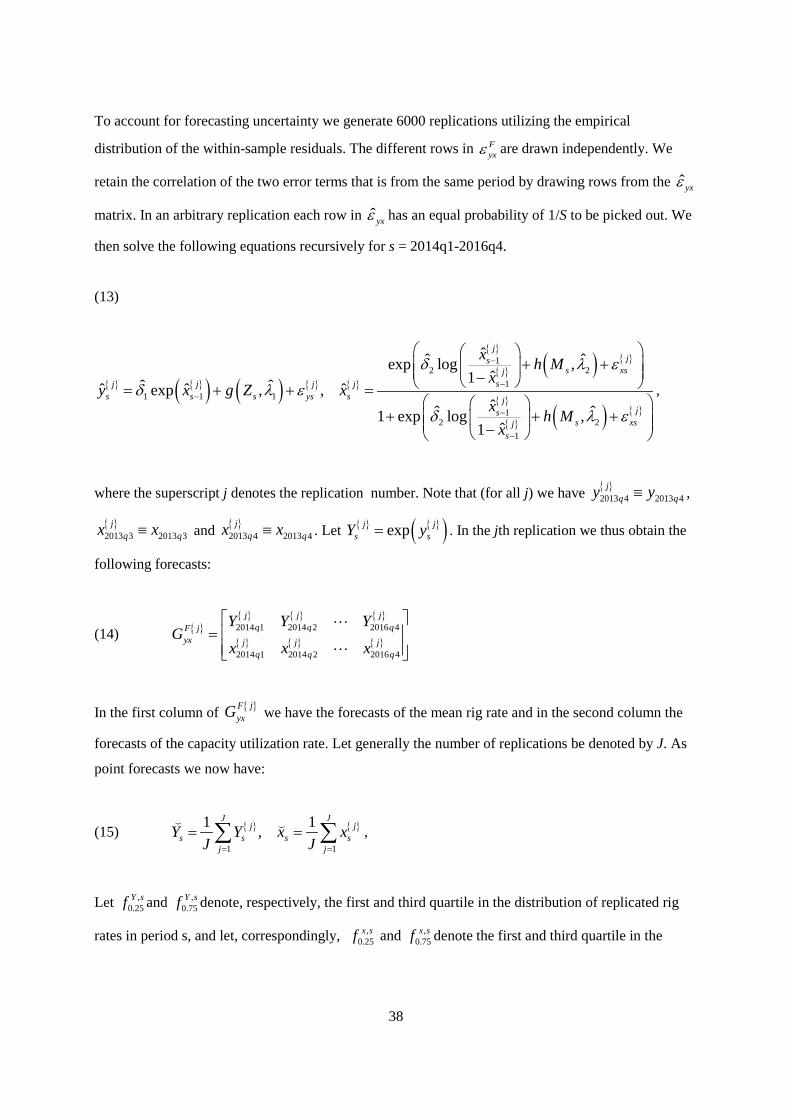
To account for forecasting uncertainty we generate 6000 replications utilizing the empirical
distribution of the within-sample residuals. The different rows in Fyxe are drawn independently. We
retain the correlation of the two error terms that is from the same period by drawing rows from the ˆyxe
matrix. In an arbitrary replication each row in ˆyxe has an equal probability of 1/S to be picked out. We
then solve the following equations recursively for s = 2014q1-2016q4.
(13)
{ } { }( ) ( ) { } { }
{ }
{ } ( ) { }
{ }
{ } ( ) { }
12 2
11 1 1
12 2
1
ˆˆ ˆexp log ,ˆ1ˆ ˆˆ ˆ ˆexp , ,ˆˆ ˆ1 exp log ,
ˆ1
jjs
s xsjsj j j j
s s s ys s jjs
s xsjs
x h Mx
y x g Z xx h M
x
δ l e
δ l e
δ l e
−
−−
−
−
+ + − = + + =
+ + + −
,
where the superscript j denotes the replication number. Note that (for all j) we have { }2013 4 2013 4
jq qy y≡ ,
{ }2013 3 2013 3
jq qx x≡ and { }
2013 4 2013 4j
q qx x≡ . Let { } { }( )expj js sY y= . In the jth replication we thus obtain the
following forecasts:
(14) { }{ } { } { }
{ } { } { }2014 1 2014 2 2016 4
2014 1 2014 2 2016 4
j j jq q qF j
yx j j jq q q
Y Y YG
x x x
=
In the first column of { }F jyxG we have the forecasts of the mean rig rate and in the second column the
forecasts of the capacity utilization rate. Let generally the number of replications be denoted by J. As
point forecasts we now have:
(15) { } { }
1 1
1 1,J J
j js s s s
j jY Y x x
J J= =
= =∑ ∑ ,
Let ,0.25Y sf and ,
0.75Y sf denote, respectively, the first and third quartile in the distribution of replicated rig
rates in period s, and let, correspondingly, ,0.25x sf and ,
0.75x sf denote the first and third quartile in the

39
distribution of replicated capacity utilization rates in the same period. The 50% bootstrapped forecast
intervals in period s are then given by:
(16) , ,0.25 0.75,Y s Y sf f and , ,
0.25 0.75,x s x sf f
with 2014 1,..., 2016q 4s q= .

Statistics Norway
Postal address:PO Box 8131 DeptNO-0033 Oslo
Offi ce address:Akersveien 26, OsloOterveien 23, Kongsvinger
E-mail: [email protected]: www.ssb.noTelephone: + 47 62 88 50 00
ISSN: 1892-753X
Desig
n: Siri B
oq
uist