modelling and opimisation of batch distillationcontrol.lth.se/documents/2000/5635.pdf · modelling...
TRANSCRIPT
ISSN 0280-5316ISRN LUTFD2/TFRT--5635--SE
Modelling and Opimisation of Batch Distillation
Anna Klingberg
Department of Automatic ControlLund Institute of Technology
January 2000

Department of Automatic ControlLund Institute of TechnologyBox 118SE-221 00 Lund Sweden
Document nameMASTER THESIS
Date of issueFebruary 2000
Document NumberISRN LUTFD2/TFRT--5635--SE
Author(s)
Anna KlingbergSupervisor
C. Löblein, Bayer AG, C.C. Pantelides, Imp.Coll.,A. Rantzer LTH
Sponsoring organisation
Title and subtitleModelling and Optimization of Batch Distillation. (Modellering och optimering av satsvis destillation.)
Abstract
The detailed dynamic modelling, simulation and optimisation of a batch distillation process at Bayer AGis presented. The model considers a mixture of 10 components separated in a 40 tray column.
Simulations performed in the process modelling tool gPROMS proved that the model gives a very accuratedescription of the process behaviour. To increase the profit of the process an optimisation of the operatingprocedure was performed, with the reflux ratio as the only control variable. The optimisation resultedin an increased profit, i.e. the product yield was increased while at the same time production timewas decreased. Another optimisation was performed to account for the periodicity of the process, byoptimising the initial conditions of the batch. These depend on the amount of fresh feed and the amountand composition of material which is recycled from the intermediate cut and mixed with the fresh feed.This optimisation also resulted in an increased profit.
Overall, gPROMS proved to be a powerful tool for solving optimisation problems of large scale models ofgreat complexity such as the batch distillation process.
Key words
Classification system and/or index terms (if any)
Supplementary bibliographical information
ISSN and key title0280–5316
ISBN
LanguageEnglish
Number of pages55
Security classification
Recipient’s notes
The report may be ordered from the Department of Automatic Control or borrowed through:University Library 2, Box 3, SE-221 00 Lund, SwedenFax +46 46 222 44 22 E-mail [email protected]

Acknowledgements 2
Acknowledgements
I would like to thank Professor Costas Pantelides for giving me the opportunity to come toImperial College and learn about gPROMS and to be able to apply these skills in anindustrially relevant context at Bayer AG.
I’m grateful to Dr Christian Löblein for arranging my stay at Bayer AG and for all the timeand effort he put into this project. Without his knowledge, help and trust the results nowobtained would not have been.
I would also like to thank the people at Process Systems Enterprise, PSE Ltd, for providingme with a gPROMS license during my stay at Bayer and especially Christian Schulz for hishelp solving arising problems when working on the simulation of the entire batch distillationmodel.
For the support in Sweden I would like to thank Professor Anders Ranzter and Professor Carl-Johan Åström, who had contacts at Imperial College.
My stay at Imperial College was financially supported by the ERASMUS program and forthis I’m very thankful.
Table of Contents 3
List of Figures 5
List of Tables 6
1. Introduction 71.1 Background.........................................................................................................71.2 Problem Statement .............................................................................................71.3 Outline of the Thesis ..........................................................................................8
2. Process Description 92.1 Components........................................................................................................92.2 The Column........................................................................................................92.3 Operation Procedure...........................................................................................9
2.3.1 Reflux Ratio...........................................................................................92.3.2 Switching Criteria During Operation...................................................112.3.3 Pressure................................................................................................12
3. The Model of the Process 133.1 Model Accuracy...............................................................................................133.2 The Structure of the Model ..............................................................................133.3 Model Assumptions .........................................................................................14
4. gPROMS 164.1 Features of gPROMS........................................................................................164.2 gOPT ................................................................................................................164.3 Limitations Using gOPT ..................................................................................17
5. The Mathematical Problem of Dynamic Optimisation 195.1 The General Form of the Dynamic Optimisation Problem..............................195.2 Solution Techniques.........................................................................................20
6. Simulation of the Batch Distillation Column 226.1 Operating Procedure.........................................................................................226.2 Initialisation .....................................................................................................226.3 Simulation of the Simplified Model.................................................................236.4 Simulation of the Detailed Model....................................................................256.5 gPROMS Performance .....................................................................................26
7. Optimisation 277.1 Off-cut and Intermediate Cut ...........................................................................277.2 Main Cut...........................................................................................................287.3 Optimisation of the Operating Procedure of the Entire Batch.........................297.4 The Summarised Results ..................................................................................32
8. Periodic Operation 338.1 Optimisation with a Multiplexer ......................................................................338.2 Optimisation of Periodic Operation.................................................................358.3 Optimisation with Fresh Feed as Time Invariant Parameter............................36
9. Conclusions and Directions for Future Work 389.1 Conclusions ......................................................................................................389.2 Directions for Future Work..............................................................................38
Table of Contents 4
Nomenclature 40
References 42
Appendix A Feed Composition 44
Appendix B The Equations of the Model 45B.1 Tray..................................................................................................................45B.2 Reboiler Drum.................................................................................................46B.3 PI-controller ....................................................................................................47B.4 Condenser........................................................................................................48B.5 Reflux Drum....................................................................................................48B.6 Divider.............................................................................................................49B.7 Accumulator ....................................................................................................50B.8 Equilibrium and Physical Properties Calculations ..........................................50
Appendix C gOPT Settings and gPROMS Performance During Optimisation 53
Appendix D gOPT Settings and gPROMS Performance During Optimisationof Periodic Operation 54
List of Figures 5
2.1 The batch distillation column.................................................................................102.2 Simulation results of the temperature in the column..............................................112.3 Concentration of C10 in the main cut accumulator ...............................................11
3.1 Flowsheet ...............................................................................................................14
4.1 Function y = ( ) 2/1tanh +xβ ..................................................................................17
5.1 Algorithm for dynamic optimisation using CVP ...................................................21
6.1 Reflux ratio and divider mass fraction profiles of simplified model at base case ...............................................................................................................24
6.2 Reflux ratio and divider mass fraction profiles of detailed model atbase case ................................................................................................................25
7.1 Reflux ratio and divider mass fraction profiles at optimum for off-cut andintermediate cut ......................................................................................................28
7.2 Reflux ratio and divider mass fraction profiles at optimum for main cut ..............297.3 Reflux ratio and divider mass fraction profiles at optimum for the
entire batch.............................................................................................................31
8.1 Reflux ratio and divider mass fraction profiles at optimum whenusing a multiplexer.................................................................................................34
8.2 Reflux ratio and divider mass fraction profiles at optimum of theperiodic operation ..................................................................................................37
8.3 Comparison of the reflux ratios .............................................................................37
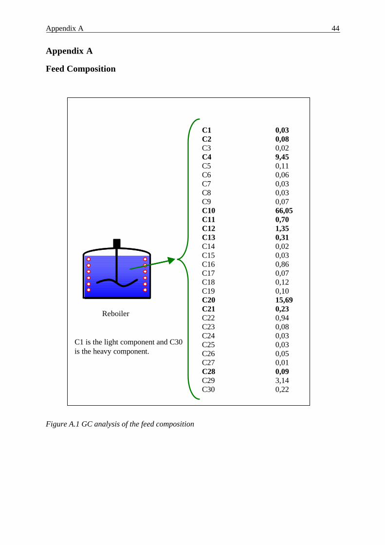
A.1 GC analysis of the feed composition......................................................................44
B.1 Tray........................................................................................................................45B.2 Reboiler Drum........................................................................................................46B.3 Condenser...............................................................................................................48B.4 Reflux Drum...........................................................................................................48B.5 Divider ...................................................................................................................49B.6 Accumulator...........................................................................................................50
List of Tables 6
2.1 The operating procedure ........................................................................................12
3.1 Components considered in the model ....................................................................15
6.1 Operating procedure during simulation..................................................................226.2 The initialisation conditions for simulation ...........................................................236.3 Feed composition for the simplified model ...........................................................246.4 Computation times of simulation...........................................................................26
7.1 Summarised results of the optimisations................................................................317.2 Summarised results of gPROMS performance during optimisation ......................31
8.1 Results of the optimisation with multiplexer compared to base case ....................348.2 gPROMS performance during optimisation with multiplexer ...............................348.3 Results of optimisation of the periodic operation compared to base case .............368.4 Results of optimisation of the periodic operation compared to base case .............37
C.1 gOPT settings and gPROMS performance during optimisations ...........................53
D.1 gOPT settings and gPROMS performance during optimisations ...........................54
1. Introduction 7
1. Introduction
1.1 Background
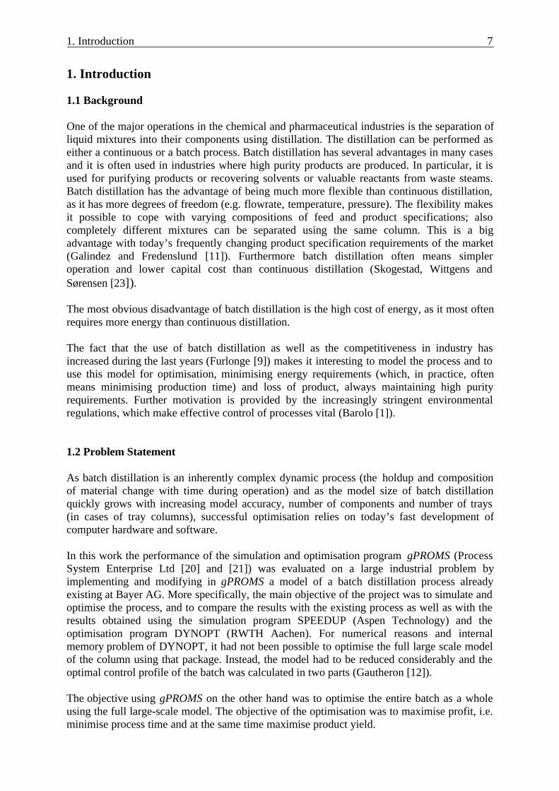
One of the major operations in the chemical and pharmaceutical industries is the separation ofliquid mixtures into their components using distillation. The distillation can be performed aseither a continuous or a batch process. Batch distillation has several advantages in many casesand it is often used in industries where high purity products are produced. In particular, it isused for purifying products or recovering solvents or valuable reactants from waste steams.Batch distillation has the advantage of being much more flexible than continuous distillation,as it has more degrees of freedom (e.g. flowrate, temperature, pressure). The flexibility makesit possible to cope with varying compositions of feed and product specifications; alsocompletely different mixtures can be separated using the same column. This is a bigadvantage with today’s frequently changing product specification requirements of the market(Galindez and Fredenslund [11]). Furthermore batch distillation often means simpleroperation and lower capital cost than continuous distillation (Skogestad, Wittgens andSørensen [23]).
The most obvious disadvantage of batch distillation is the high cost of energy, as it most oftenrequires more energy than continuous distillation.
The fact that the use of batch distillation as well as the competitiveness in industry hasincreased during the last years (Furlonge [9]) makes it interesting to model the process and touse this model for optimisation, minimising energy requirements (which, in practice, oftenmeans minimising production time) and loss of product, always maintaining high purityrequirements. Further motivation is provided by the increasingly stringent environmentalregulations, which make effective control of processes vital (Barolo [1]).
1.2 Problem Statement
As batch distillation is an inherently complex dynamic process (the holdup and compositionof material change with time during operation) and as the model size of batch distillationquickly grows with increasing model accuracy, number of components and number of trays(in cases of tray columns), successful optimisation relies on today’s fast development ofcomputer hardware and software.
In this work the performance of the simulation and optimisation program gPROMS (ProcessSystem Enterprise Ltd [20] and [21]) was evaluated on a large industrial problem byimplementing and modifying in gPROMS a model of a batch distillation process alreadyexisting at Bayer AG. More specifically, the main objective of the project was to simulate andoptimise the process, and to compare the results with the existing process as well as with theresults obtained using the simulation program SPEEDUP (Aspen Technology) and theoptimisation program DYNOPT (RWTH Aachen). For numerical reasons and internalmemory problem of DYNOPT, it had not been possible to optimise the full large scale modelof the column using that package. Instead, the model had to be reduced considerably and theoptimal control profile of the batch was calculated in two parts (Gautheron [12]).
The objective using gPROMS on the other hand was to optimise the entire batch as a wholeusing the full large-scale model. The objective of the optimisation was to maximise profit, i.e.minimise process time and at the same time maximise product yield.
1. Introduction 8
1.3 Outline of the Thesis
Section 2 gives an overview of the process considered. The operating procedure, the feedmixture and the design of the column are described.
The detailed model of the batch distillation is then presented in section 3 and the gPROMStool used to simulate and optimise this model is briefly described in section 4. Themathematical problem that is solved in gPROMS and the solution techniques used bygPROMS for the task are further outlined in section 5.
Results from the simulations and optimisations performed are presented in sections 6 and 7respectively.
Section 8 describes the optimisation of periodic operation and presents the results obtained.
Finally conclusions are drawn and directions for future work are given in section 9.
2. Process Description 9
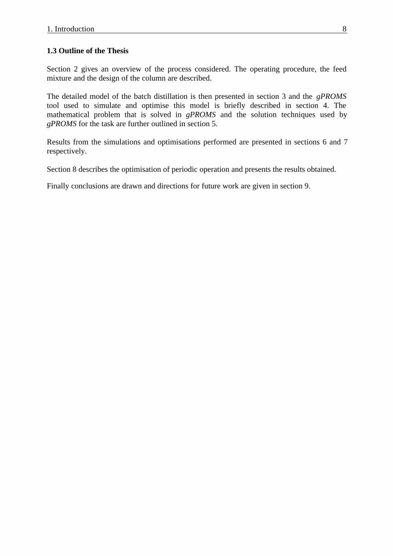
2. Process Description
2.1 Components
The objective of the process considered is to produce C10. More specifically, starting with afeed mixture of over 30 components with an initial concentration of C10 of about 66%, thegoal is a product purity of at least 98.5% C10. An example of a gas chromatography analysisof the feed is shown in appendix A.
2.2 The Column
Both a tray and a packed column are used for the separation of the mixture described above.Because of time limitation only the tray column has been considered in this work. The traycolumn which is used to perform the desired separation consists of 40 trays. Each tray hasabout 70 bubble caps and the column is about 13.5 meters high with a diameter of 1 meter.The process is schematically described in figure 2.1.
2.3 Operation Procedure
For the purposes of this thesis, the duration of the process is normalised, with 100%corresponding to 100 hours of nominal operation. The pressure difference used to regulate theproduction is also normalised.
2.3.1 Reflux Ratio
The operating policy used is a piecewise constant reflux ratio, i.e. the reflux ratio is fixed at apre-defined value during the different time intervals of the process. This causes the distillatecomposition to change during the operation, as the composition of the mixture in the reboilerchanges.
The operating schedule of the reflux ratio consists of five different cuts:
1. Light component off-cut:The light components are evacuated. This takes 5 hours with the reflux ratio, R=1.
2. Off-cut:A lighter component (C4) in the mixture is removed without specification. The duration ofthis cut is 14 hours with reflux ratio R=5.
3. Intermediate cut:The mass fraction of C10 should reach 98.4% by the end of this phase. This is achieved byusing a reflux ratio of 10 over 16 hours.
4. Main cut:The mass fraction of C10 in the product accumulator should reach at least 98.5% by theend of this phase. The reflux ratio is kept at 5 over 7 hours, and is then switched to 8 foran additional 54 hours.
5. Heavy component off-cut:The heavy components are evacuated with maximum pressure and minimum reflux ratio(R=0). This phase takes 4 hours.
2. Process Description 10
Reboiler
Condenser
Divider :Reflux ratio R
Steam
Condensate
Intermediatecut
Off-cut &heavy
componentoff-cut
Process operatorPC
Main cut
Objective:C10
98.5 %
Accumulators
The intermediate cut is mixed with the next feed.
Lightcomponent off-
cut
Tray column
Reflux Drum
Figure 2.1 The batch distillation column.
2. Process Description 11
The whole operation takes 100 hours.
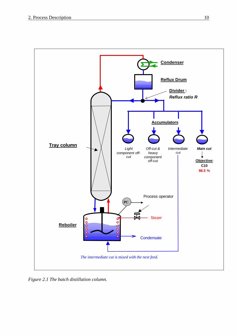
2.3.2 Switching Criteria During Operation
The temperature in the column is measured during the operation. An example of a simulationof the temperature in the column is shown below (figure 2.2).
Figure 2.2 Simulation results of the temperature in the column.
The two parts with the steep gradient that can be observed in the plot tell the process operatorwhen the off-cut and the intermediate cut begin.
A melting point analysis of the product shows the process operator when the concentration ofC10 has reached the concentration constraint of 98.4% in the divider and the main cut canstart. The analysis of the mixture composition could alternatively be done using gaschromatography (GC). However, the melting point analysis is much faster than a GC-analysis,taking about 5 min compared to 30 min for the GC-analysis, and the correlation between themelting point and the concentration has been proved to be good (Gautheron [12]).
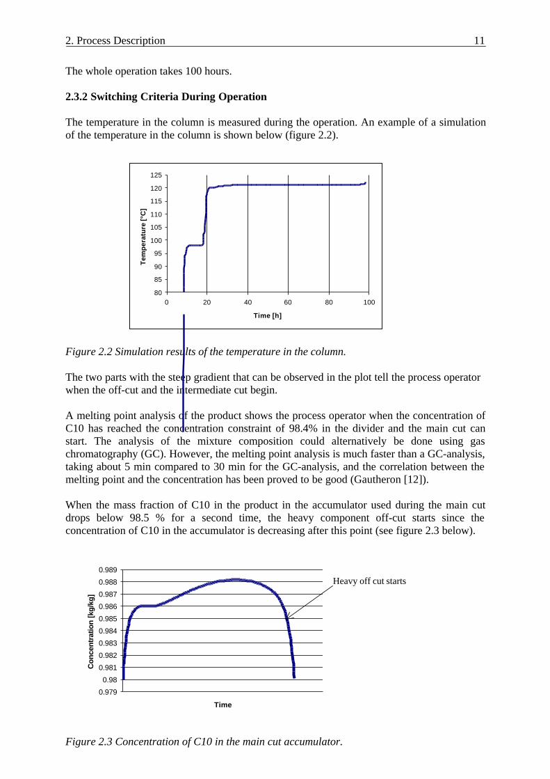
When the mass fraction of C10 in the product in the accumulator used during the main cutdrops below 98.5 % for a second time, the heavy component off-cut starts since theconcentration of C10 in the accumulator is decreasing after this point (see figure 2.3 below).
Figure 2.3 Concentration of C10 in the main cut accumulator.
Heavy off cut starts
0.979
0.98
0.981
0.982
0.983
0.984
0.985
0.986
0.987
0.988
0.989
Time
Con
cent
ratio
n [k
g/kg
]
80
85
90
95
100
105
110
115
120
125
0 20 40 60 80 100
Time [h]
Tem
per
atu
re [°
C]
2. Process Description 12
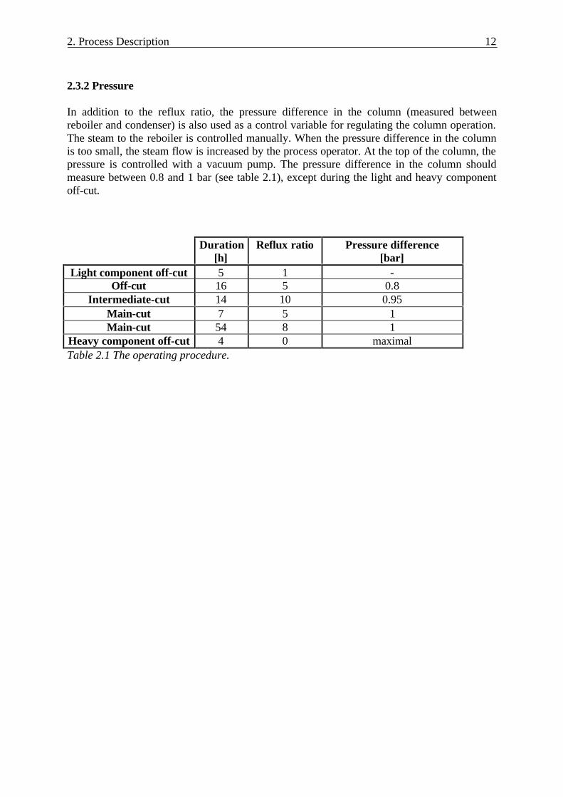
2.3.2 Pressure
In addition to the reflux ratio, the pressure difference in the column (measured betweenreboiler and condenser) is also used as a control variable for regulating the column operation.The steam to the reboiler is controlled manually. When the pressure difference in the columnis too small, the steam flow is increased by the process operator. At the top of the column, thepressure is controlled with a vacuum pump. The pressure difference in the column shouldmeasure between 0.8 and 1 bar (see table 2.1), except during the light and heavy componentoff-cut.
Duration[h]
Reflux ratio Pressure difference[bar]
Light component off-cut 5 1 -Off-cut 16 5 0.8
Intermediate-cut 14 10 0.95Main-cut 7 5 1Main-cut 54 8 1
Heavy component off-cut 4 0 maximalTable 2.1 The operating procedure.
3. The Model of the Process 13
3. The Model of the Process
3.1 Model Accuracy
In general, increased model accuracy comes at the expense of increased model complexity.and decreased computational efficiency. This means that the size of the models used inpractice has to be a compromise between accuracy and simplicity to avoid numerical problemand to retain computational efficiency.
The so-called “short-cut” models for batch distillation have been very widely used in theliterature. Short-cut techniques develop a direct relationship between the composition in thereboiler drum and the distillate, thus avoiding the modelling of individual trays. This leads toa significant reduction in model size. This further means that the computational effort isreduced, which was of crucial importance before today’s powerful computer hardwarebecame available (Diwekar [7]).
Much research on batch distillation has also been done using models built up by severalsimplified sub models, with common assumptions such as constant liquid holdup on the tray,negligible vapour holdup, constant molal overflow (neglecting the energy balance and liquidhydraulics on each tray) and ideal equilibrium stages. Some of the assumptions can, however,cause the models to give answers far from the truth (Furlonge [10]). The usefulness of themodels is reduced, potentially leading to inaccurate decisions concerning operation or design,if the knowledge of the assumptions is not good enough (Nilsson [16]).
In the case of batch distillation, the problem of model mismatch is aggravated by the“integrating” nature of the batch process. Structural or parametric errors in the model causesthe error in predicted composition to increase in magnitude throughout the duration of asimulated batch run. This is fundamental to the process, and is true for any model solutiontechnique (Bosley [4]).
With the latest computational capacity currently available at hand, it was possible to make useof a process model that is more detailed than most other models used for similar purposes.
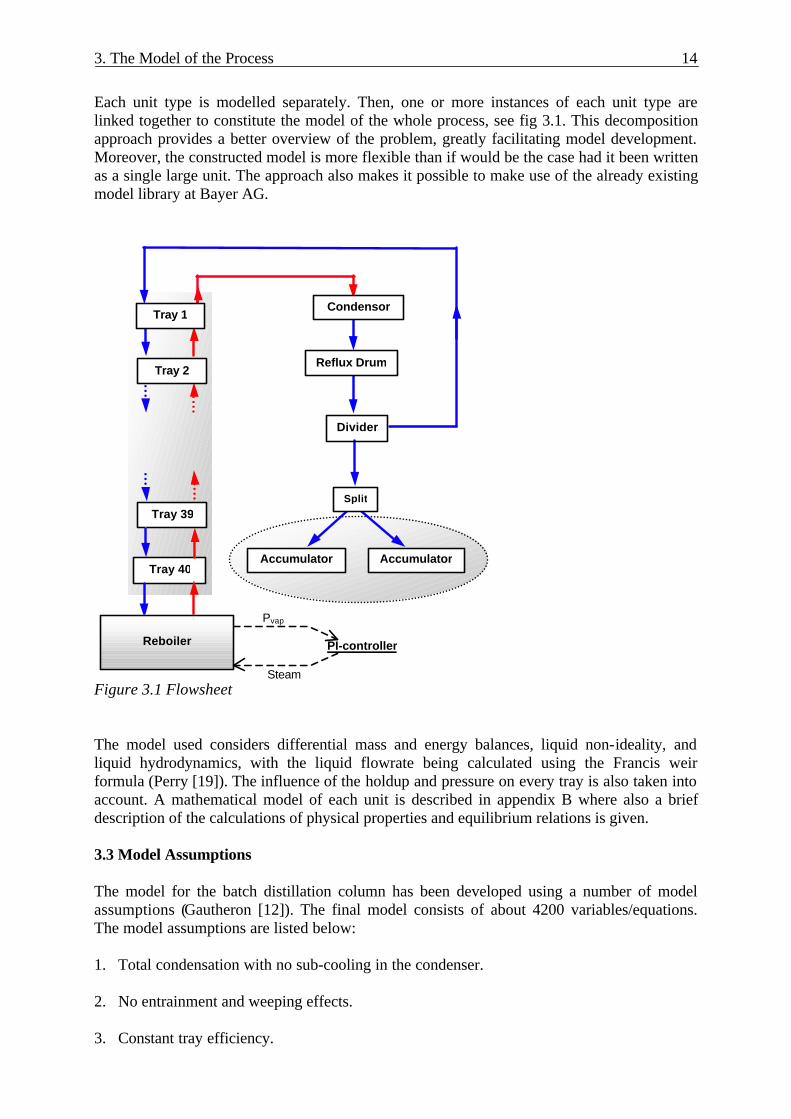
3.2 The Structure of the Model
The model consists of seven different units:
• Tray
• Reboiler drum
• PI-controller
• Condenser
• Reflux drum
• Divider
• Accumulator
3. The Model of the Process 14
Each unit type is modelled separately. Then, one or more instances of each unit type arelinked together to constitute the model of the whole process, see fig 3.1. This decompositionapproach provides a better overview of the problem, greatly facilitating model development.Moreover, the constructed model is more flexible than if would be the case had it been writtenas a single large unit. The approach also makes it possible to make use of the already existingmodel library at Bayer AG.
Figure 3.1 Flowsheet
The model used considers differential mass and energy balances, liquid non-ideality, andliquid hydrodynamics, with the liquid flowrate being calculated using the Francis weirformula (Perry [19]). The influence of the holdup and pressure on every tray is also taken intoaccount. A mathematical model of each unit is described in appendix B where also a briefdescription of the calculations of physical properties and equilibrium relations is given.
3.3 Model Assumptions
The model for the batch distillation column has been developed using a number of modelassumptions (Gautheron [12]). The final model consists of about 4200 variables/equations.The model assumptions are listed below:
1. Total condensation with no sub-cooling in the condenser.
2. No entrainment and weeping effects.
3. Constant tray efficiency.
Reflux Drum
Accumulator AccumulatorTray 40
Tray 39
PI-controller
Pvap
Steam
Tray 1
Tray 2
Split
Condensor
Divider
Reboiler
3. The Model of the Process 15
4. Adiabatic operation.
5. Phase equilibrium.
6. Perfect mixing on the trays and in the reboiler drum.
7. Ideal vapour phase.
At the beginning of the simulation, it is assumed that the material held on the trays of thecolumn contains only the light key component. This is more accurate than the commonly usedassumption that the initial concentration in the whole column is the same as that of the feed.The latter assumption has, however, been proved to be of acceptable accuracy (Sadomoto andMiyahara [22]).
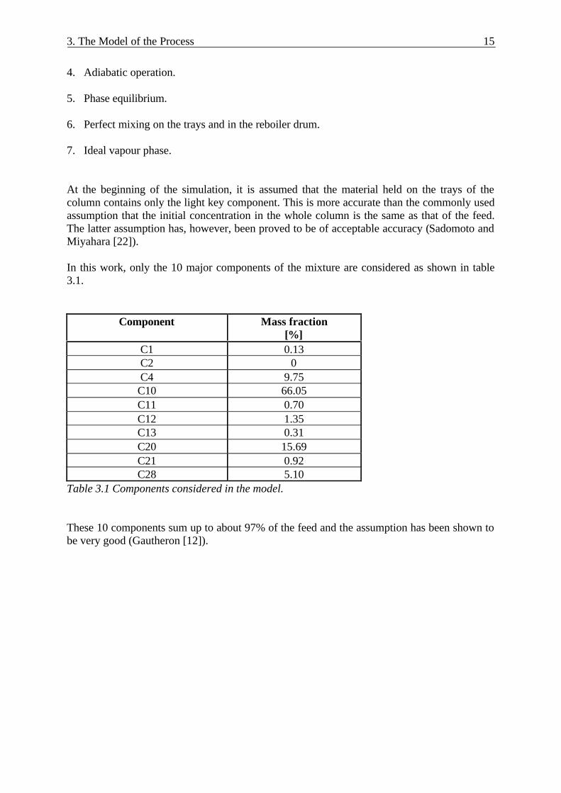
In this work, only the 10 major components of the mixture are considered as shown in table3.1.
Component Mass fraction[%]
C1 0.13C2 0C4 9.75C10 66.05C11 0.70C12 1.35C13 0.31C20 15.69C21 0.92C28 5.10
Table 3.1 Components considered in the model.
These 10 components sum up to about 97% of the feed and the assumption has been shown tobe very good (Gautheron [12]).
4. gPROMS 16
4. gPROMS
4.1 Features of gPROMS
gPROMS (general PROcess Modelling System) process modelling software tool that is wellsuited for the dynamic modelling, simulation and optimisation of chemical processes. One ofthe reasons for this is its ability to model and handle discontinuities of the types that veryoften occurs in chemical processes (for example, when changing the reflux ratio during adistillation operation).
gPROMS distinguishes three fundamental types of modelling entity. MODELs describe thechemical and physical behaviour of the system, defined by the equations that have beenspecified by the user, while TASKs are descriptions of the external actions and disturbancesimposed on the system. Especially when dealing with batch processes, the modelling ofoperating procedures is of great importance. Such operating procedures are very easilydescribed as TASK entities, as the gPROMS TASK language provides a large variety offeatures, with actions being executed in sequence or in parallel, conditionally or iteratively,thus describing the operation of the process in a very general and flexible way. The third typeof entity is the PROCESS, which is formed by a TASK driving a MODEL with some additionalinformation, such as initial conditions and the time variation of the input variables. Thus, asimulation is defined as the execution of such a PROCESS.
As with any other chemical process, the modelling of batch distillation requires the accurateconsideration of physical properties in order to model the thermodynamics of the process inan accurate manner. This work has made use of the IKCAPE physical properties package forthis purpose. This package has been interfaced to gPROMS via the gPROMS Foreign ObjectInterface (gPROMS Introductory User Guide [21]).
Version 1.7 of gPROMS was used throughout this study.
4.2 gOPT
Dynamic optimisation in gPROMS is performed by gOPT, which is an interface to thedynamic optimisation code DAEOPT (Vassiliadis et al. [24] and [25]). The gPROMS inputfile for simulation can be used in gOPT without any modifications. Some additionalinformation that specifically concerns the definition of the optimisation problem has to bespecified in a separate input file. This information includes the specification of the objectivefunction and the various constraints that the optimal solution has to satisfy, the time horizonof the operation to be optimised, the control variables to be manipulated by the optimisationas well as the allowable forms of time-variation for these controls.
The user also has the option of specifying various parameters that affect the numericalperformance of the optimisation. This is done by creating a parameter file which typicallyspecifies various tolerances (relative and absolute DAE integration tolerance, steady statetolerance and optimisation tolerance) and also allows the setting of a flag that instructs gOPTto use a quicker but slightly less reliable method for calculating sensitivities. If no suchparameter file is provided by the user, the gOPT solver will use default values for all of theparameters.
4. gPROMS 17
4.3 Limitations Using gOPT
The gOPT solver cannot handle directly discontinuities described by conditional equations (IFstatements). Therefore, any conditional equation used for the simulation has to bereformulated before the simulation input file is used for optimisation.
In some cases, this can be done using the MAX operator. This is illustrated in the followingexample:
IF B + C > 0 THENA = B + C
ELSEA = 0
may be reformulated as:
MAX(A,0) = B+C
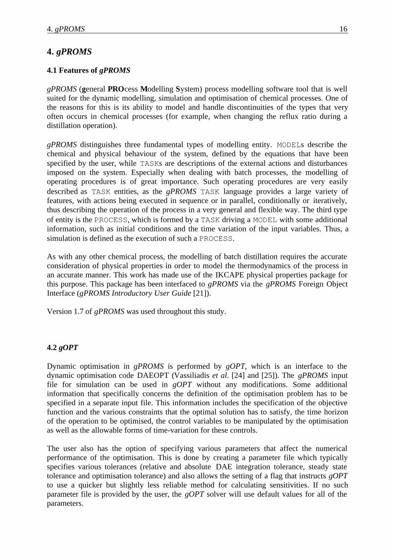
Another option is to use the ( ) 2/1tanh +xβ function. As the positive parameter β grows, thisfunction is an increasingly accurate approximation of a discontinuous unit step function:
Figure 4.1 Function y = ( ) 2/1tanh +xβ
0
0.1
0.2
0.3
0.4
0.5
0.6
0.7
0.8
0.9
1
β=1
β=10β=100
4. gPROMS 18
An example of how to use the above function to reformulate an IF statement is shown below:
IF X > 0.5 THENB = 2.5
ELSEB = 1.3
may be reformulated in terms of the following equations:
B = 2.5*A1 + 1.3*A2A1 = (1 + tanh(β*(x-0.5)))/2A2 = (1 - tanh(β*(x-0.5)))/2
Here we have introduced two new variables, A1 and A2. Note that, if x is sufficiently largerthan 0.5, then A1≈1 and A2≈0; therefore, the first equation makes B ≈2.5. On the other hand,if x is sufficiently smaller than 0.5, then A1≈0 and A2≈1; and therefore B ≈1.3.
In fact, this type of reformulation may be generalised to any conditional equation described byan IF statement. Consider the general conditional equation:
IF g(x) > 0 THENf1(x) = 0
ELSEf2(x) = 0
where g(x), f1(x) and f2(x) are general functions of a vector of variables x. This can bereformulated in terms of the continuous equations:
A1*f1(x) + A2*f2(x) = 0A1 = (1 + tanh(β*g(x)))/2A2 = (1 - tanh(β*g(x)))/2
5. The Mathematical Problem of Dynamic Optimisation 19
5. The Mathematical Problem of Dynamic Optimisation
5.1 The General Form of the Dynamic Optimisation Problem
The mathematical model of a chemical process is usually described by a set of differential andalgebraic equations, often abbreviated as DAEs. These equations can be written in thefollowing way:
( ) ( ) ( ) ( ) 0,,,, =
•
vtutytxtxf [ ]ftt ,0∈∀ (5:1)
where x(t) = differential (“state”) variables .x(t ) = time derivatives of the differential variables
y(t) = algebraic variables
u(t) = control variables
v = time invariant parameters
tf = time horizon of interest
To solve the above equation system, initial conditions need to be given. These can bedescribed by a set of general non-linear relations:
( ) ( ) ( ) ( ) 0,0,0,,0 =
•
vuytxxI (5:2)
Suitable initial conditions for optimisation of batch distillation are initial holdup, temperatureand composition throughout the column (Furlonge [9]).
Optimisation in gPROMS aims to determine the time profile (or trajectory) of the controlvariables and/or the values of the time-invariant parameters which maximise or minimise aspecified objective function while at the same time satisfying any imposed constraints. Theseconstraints could be path constraints, interior point constraints or end-point constraints.
Path constraints are defined during the whole time horizon and may be written as:
( ) ( ) ( ) ( ) 0,,,,, ≤
•
tvtutytxtxh [ ]ftt ,0∈∀ (5:3)
Interior point constraints are only defined at particular instances in time:
( ) ( ) ( ) ( ) 0,,,,, ≤
•
λλλλλ tvtutytxtxg ,...2,1=λ (5:4)
End-point constraints are those that must be satisfied at the final time of the operation.
5. The Mathematical Problem of Dynamic Optimisation 20
For a minimisation problem, the objective function is of the general form:
( ) ( ) ( ) ( )
Φ
•
fffff tvtutytxtx ,,,,,min (5:5)
5.2 Solution Techniques
The solution technique used for optimisation in gOPT is called control vectorparameterisation (CVP). The CVP method employs a parameterisation of the control variablesu(t), assuming that they are described as a particular class of functions of time (for example,piecewise constant or piecewise linear functions) expressed in terms of a finite number ofparameters.
At each optimisation iteration, the optimiser specifies certain values for the optimisationdecision variables; the latter comprise both the parameters describing the control profiles u(t),and the time-invariant parameters v. An integration of the DAE system can then be performedover the whole time horizon to evaluate the constraints and the objective function. The partialderivatives of these quantities with respect to the optimisation decision variables can also beevaluated during this integration if required by the optimiser.
The solution method using CVP is made as efficient as possible by adjustment of the timestep and the order of integration method during each integration. The algorithm for dynamicoptimisation using CVP is shown in fig 5.1 (taken from Furlonge [9]).
The repeated integration of the DAE system could be avoided by use of collocationtechniques, where the state and algebraic variables are discretised as well (Logsdon andBiegler [15]) and a non-linear optimisation problem is then solved. However, this often leadsto extremely large non-linear optimisation problems with thousands of equations which mightbe difficult to solve.
5. The Mathematical Problem of Dynamic Optimisation 21
Initial guesses of optimisation decision variables(µ = parameter of control
variable parameterisationv = time-invariant parameters
tf = time horizon)
Figure 5.1 Algorithm for dynamic optimisation using CVP.
NLP(nonlinearprogramming)
step
Evaluation ofobjective function
and constraints
Areoptimality conditions
satisfied?
END
Yes
No
New values for(µ, v, tf)
Initialisation andintegration of
DAE
6. Simulation of the Batch Distillation Coulmn 22
6. Simulation of the Batch Distillation Column
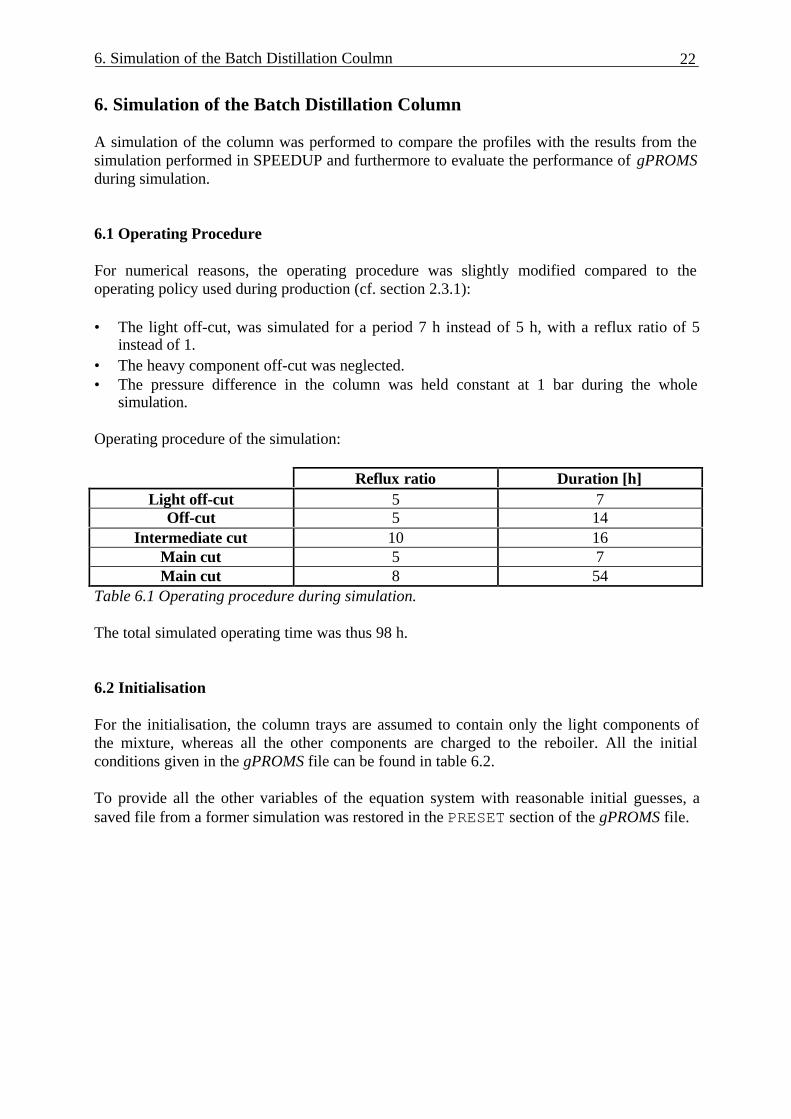
A simulation of the column was performed to compare the profiles with the results from thesimulation performed in SPEEDUP and furthermore to evaluate the performance of gPROMSduring simulation.
6.1 Operating Procedure
For numerical reasons, the operating procedure was slightly modified compared to theoperating policy used during production (cf. section 2.3.1):
• The light off-cut, was simulated for a period 7 h instead of 5 h, with a reflux ratio of 5instead of 1.
• The heavy component off-cut was neglected.• The pressure difference in the column was held constant at 1 bar during the whole
simulation.
Operating procedure of the simulation:
Reflux ratio Duration [h]Light off-cut 5 7
Off-cut 5 14Intermediate cut 10 16
Main cut 5 7Main cut 8 54
Table 6.1 Operating procedure during simulation.
The total simulated operating time was thus 98 h.
6.2 Initialisation
For the initialisation, the column trays are assumed to contain only the light components ofthe mixture, whereas all the other components are charged to the reboiler. All the initialconditions given in the gPROMS file can be found in table 6.2.
To provide all the other variables of the equation system with reasonable initial guesses, asaved file from a former simulation was restored in the PRESET section of the gPROMS file.
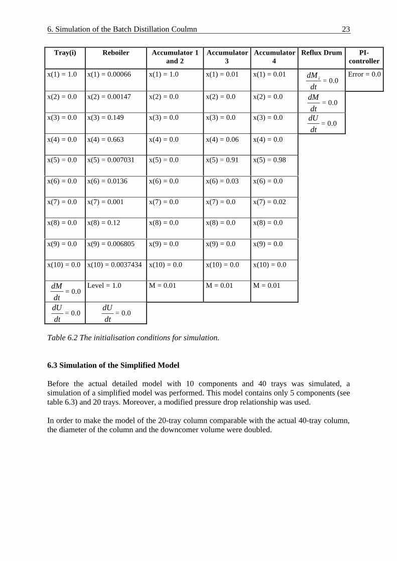
6. Simulation of the Batch Distillation Coulmn 23
Tray(i) Reboiler Accumulator 1and 2
Accumulator3
Accumulator4
Reflux Drum PI-controller
x(1) = 1.0 x(1) = 0.00066 x(1) = 1.0 x(1) = 0.01 x(1) = 0.01
dtdM i = 0.0
Error = 0.0
x(2) = 0.0 x(2) = 0.00147 x(2) = 0.0 x(2) = 0.0 x(2) = 0.0
dtdM
= 0.0
x(3) = 0.0 x(3) = 0.149 x(3) = 0.0 x(3) = 0.0 x(3) = 0.0
dtdU
= 0.0
x(4) = 0.0 x(4) = 0.663 x(4) = 0.0 x(4) = 0.06 x(4) = 0.0
x(5) = 0.0 x(5) = 0.007031 x(5) = 0.0 x(5) = 0.91 x(5) = 0.98
x(6) = 0.0 x(6) = 0.0136 x(6) = 0.0 x(6) = 0.03 x(6) = 0.0
x(7) = 0.0 x(7) = 0.001 x(7) = 0.0 x(7) = 0.0 x(7) = 0.02
x(8) = 0.0 x(8) = 0.12 x(8) = 0.0 x(8) = 0.0 x(8) = 0.0
x(9) = 0.0 x(9) = 0.006805 x(9) = 0.0 x(9) = 0.0 x(9) = 0.0
x(10) = 0.0 x(10) = 0.0037434 x(10) = 0.0 x(10) = 0.0 x(10) = 0.0
dtdM
= 0.0Level = 1.0 M = 0.01 M = 0.01 M = 0.01
dtdU
= 0.0dtdU
= 0.0
Table 6.2 The initialisation conditions for simulation.
6.3 Simulation of the Simplified Model
Before the actual detailed model with 10 components and 40 trays was simulated, asimulation of a simplified model was performed. This model contains only 5 components (seetable 6.3) and 20 trays. Moreover, a modified pressure drop relationship was used.
In order to make the model of the 20-tray column comparable with the actual 40-tray column,the diameter of the column and the downcomer volume were doubled.
6. Simulation of the Batch Distillation Coulmn 24
Component Mass fraction[%]
C1 0.13C4 9.75C10 66.75C12 1.35C20 22.02
Table 6.3 Feed composition for the simplified model.
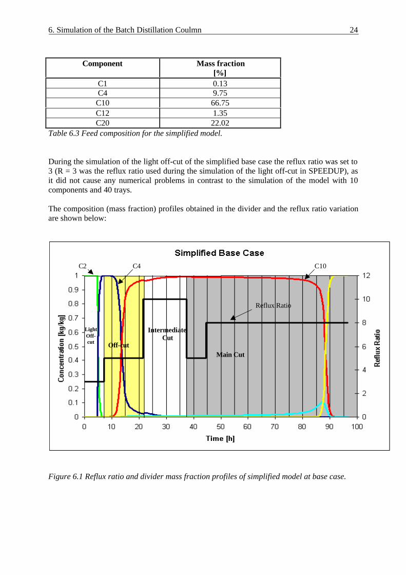
During the simulation of the light off-cut of the simplified base case the reflux ratio was set to3 (R = 3 was the reflux ratio used during the simulation of the light off-cut in SPEEDUP), asit did not cause any numerical problems in contrast to the simulation of the model with 10components and 40 trays.
The composition (mass fraction) profiles obtained in the divider and the reflux ratio variationare shown below:
Figure 6.1 Reflux ratio and divider mass fraction profiles of simplified model at base case.
LightOff-cut Off-cut
Intermediate Cut
Main Cut
Reflux Ratio
C10C4C2
6. Simulation of the Batch Distillation Coulmn 25
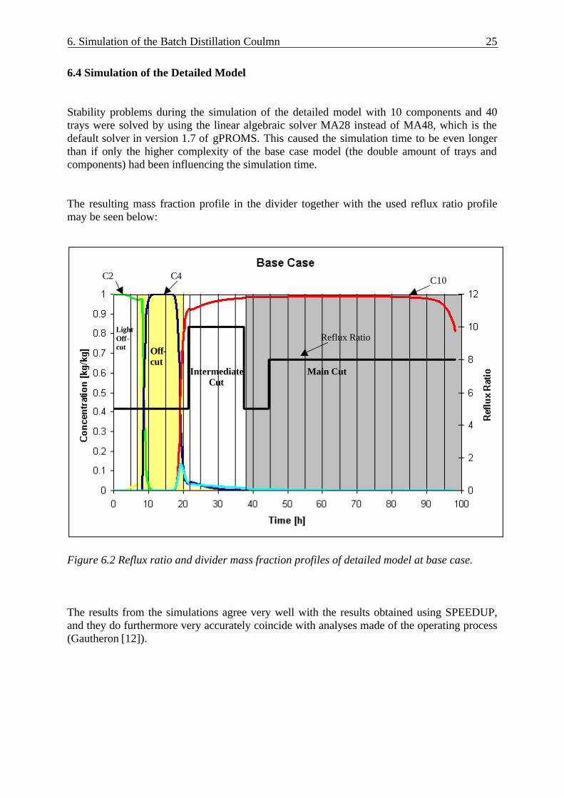
6.4 Simulation of the Detailed Model
Stability problems during the simulation of the detailed model with 10 components and 40trays were solved by using the linear algebraic solver MA28 instead of MA48, which is thedefault solver in version 1.7 of gPROMS. This caused the simulation time to be even longerthan if only the higher complexity of the base case model (the double amount of trays andcomponents) had been influencing the simulation time.
The resulting mass fraction profile in the divider together with the used reflux ratio profilemay be seen below:
Figure 6.2 Reflux ratio and divider mass fraction profiles of detailed model at base case.
The results from the simulations agree very well with the results obtained using SPEEDUP,and they do furthermore very accurately coincide with analyses made of the operating process(Gautheron [12]).
LightOff-cut Off-
cutIntermediate
CutMain Cut
Reflux Ratio
C10C2 C4
6. Simulation of the Batch Distillation Coulmn 26
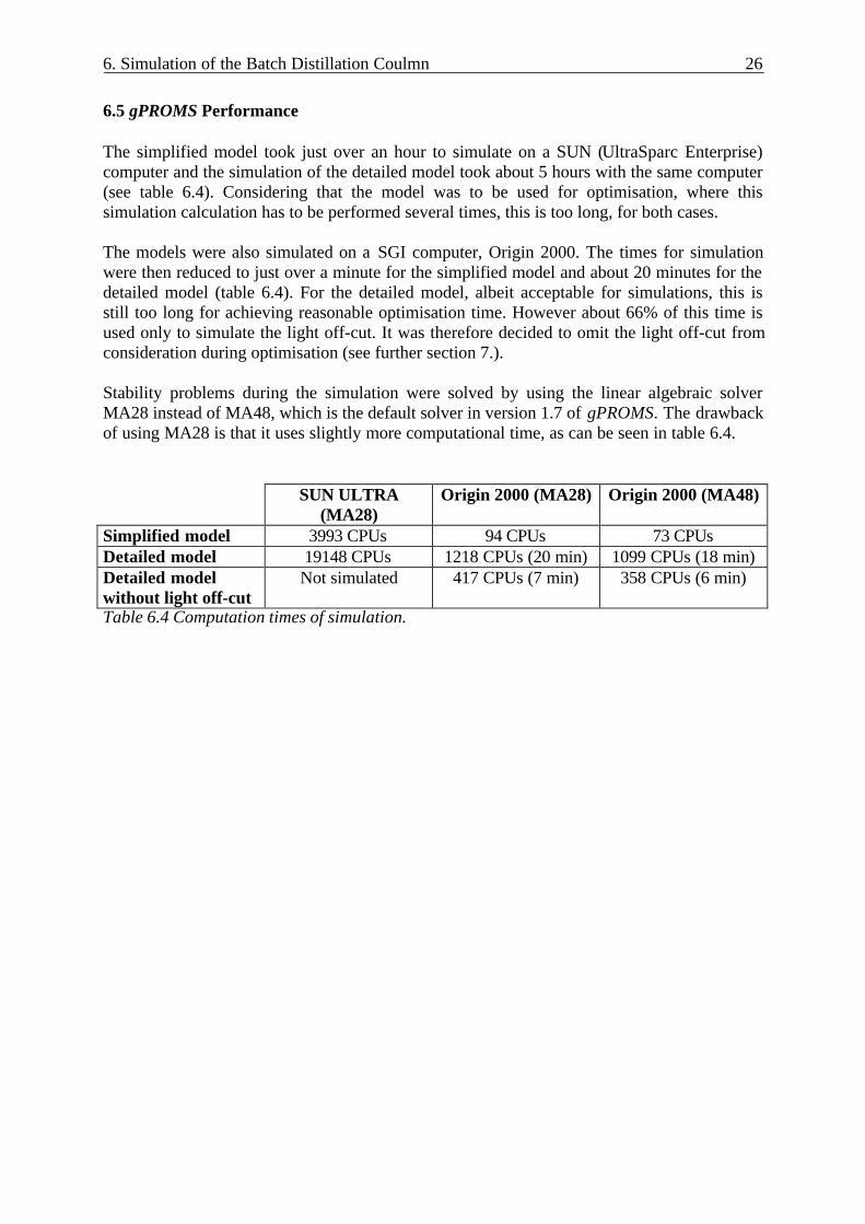
6.5 gPROMS Performance
The simplified model took just over an hour to simulate on a SUN (UltraSparc Enterprise)computer and the simulation of the detailed model took about 5 hours with the same computer(see table 6.4). Considering that the model was to be used for optimisation, where thissimulation calculation has to be performed several times, this is too long, for both cases.
The models were also simulated on a SGI computer, Origin 2000. The times for simulationwere then reduced to just over a minute for the simplified model and about 20 minutes for thedetailed model (table 6.4). For the detailed model, albeit acceptable for simulations, this isstill too long for achieving reasonable optimisation time. However about 66% of this time isused only to simulate the light off-cut. It was therefore decided to omit the light off-cut fromconsideration during optimisation (see further section 7.).
Stability problems during the simulation were solved by using the linear algebraic solverMA28 instead of MA48, which is the default solver in version 1.7 of gPROMS. The drawbackof using MA28 is that it uses slightly more computational time, as can be seen in table 6.4.
SUN ULTRA(MA28)
Origin 2000 (MA28) Origin 2000 (MA48)
Simplified model 3993 CPUs 94 CPUs 73 CPUsDetailed model 19148 CPUs 1218 CPUs (20 min) 1099 CPUs (18 min)Detailed modelwithout light off-cut
Not simulated 417 CPUs (7 min) 358 CPUs (6 min)
Table 6.4 Computation times of simulation.
7. Optimisation 27
7. Optimisation
The objective of the optimisation was to maximise the profit, i.e. to maximise the yield of C10and minimise production time.
The optimisation of the process using DYNOPT was only possible using the simplifiedmodel. In order to be able to make an accurate comparison of the optimisation results, ideallythe optimisation should have been performed using both models. However since the objectiveof this work was to consider the optimisation of the entire batch of the detailed model as abenchmark for the evaluation of the performance of gPROMS/gOPT, only the detailed modelwas optimised.
As already mentioned, the time for simulation of the whole batch was too long to achievereasonable optimisation times. Therefore the light off-cut was not considered, which reducesthe simulation time by about 66%. The heavy component off-cut was not considered, as it isalready performed in the quickest way possible, i.e. maximal steam pressure to the reboilerand no reflux. Both of these simplifications were made when optimising in DYNOPT as well.
The optimisation was first performed in two steps, like it had been done using DYNOPT. Thefirst step was to optimise the off-cut and the intermediate cut. The column was then initialisedwith the state variables at the end of the intermediate cut, and the main cut was optimised overthe remaining time horizon. After the two parts had been optimised separately, the operationwas also optimised in a single run. The only control variable during the optimisations was thereflux ratio. The base case profile of the reflux ratio was always used as the initial guess.
7.1 Off-cut and Intermediate Cut Optimisation
The off-cut and the intermediate cut were optimised with the objective of minimising the lossof C10 and the production time. At the end of the intermediate cut, the mass fraction of C10from the divider has to exceed 98.4%; this was the only endpoint-constraint imposed on theoptimisation.
The objective function to be minimised was formulated as:
Cost = tprod/t*prod + MC10/ M*C10 (7:1)
where:
tprod = production time [h]
t*prod = production time before optimisation = 30 [h]
MC10 = C10 in intermediate cut [kg]
M*C10 = C10 in intermediate cut at base case = 1333 [kg]
The computation time used for optimisation was 11064 CPUs (about 3 h) using 13optimisation iterations to find the optimum.
The optimal profile with 6 different intervals of reflux ratios results in a new production timeof 21 h, which compared with the 30 h used in the base case, represents an improvement of
7. Optimisation 28
Optimised Off-cut & Intermediate cut
0
0.1
0.2
0.3
0.4
0.5
0.6
0.7
0.8
0.9
1
0 5 10 15 20
Time [h]
Co
nce
ntr
atio
n [
kg/k
g]
0
5
10
15
20
Ref
lux
rati
o
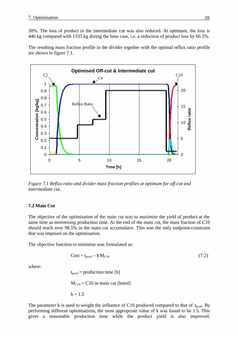
30%. The loss of product in the intermediate cut was also reduced. At optimum, the loss is446 kg compared with 1333 kg during the base case, i.e. a reduction of product loss by 66.5%.
The resulting mass fraction profile in the divider together with the optimal reflux ratio profileare shown in figure 7.1.
Figure 7.1 Reflux ratio and divider mass fraction profiles at optimum for off-cut andintermediate cut.
7.2 Main Cut
The objective of the optimisation of the main cut was to maximise the yield of product at thesame time as minimising production time. At the end of the main cut, the mass fraction of C10should reach over 98.5% in the main cut accumulator. This was the only endpoint-constraintthat was imposed on the optimisation.
The objective function to minimise was formulated as:
Cost = tprod – k.MC10 (7:2)
where:tprod = production time [h]
MC10 = C10 in main cut [kmol]
k = 1.5
The parameter k is used to weight the influence of C10 produced compared to that of tprod. Byperforming different optimisations, the most appropriate value of k was found to be 1.5. Thisgives a reasonable production time while the product yield is also improved.
Reflux Ratio
C10C2C4
7. Optimisation 29
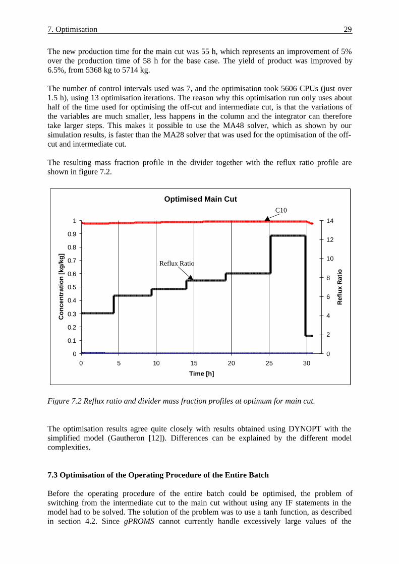
The new production time for the main cut was 55 h, which represents an improvement of 5%over the production time of 58 h for the base case. The yield of product was improved by6.5%, from 5368 kg to 5714 kg.
The number of control intervals used was 7, and the optimisation took 5606 CPUs (just over1.5 h), using 13 optimisation iterations. The reason why this optimisation run only uses abouthalf of the time used for optimising the off-cut and intermediate cut, is that the variations ofthe variables are much smaller, less happens in the column and the integrator can thereforetake larger steps. This makes it possible to use the MA48 solver, which as shown by oursimulation results, is faster than the MA28 solver that was used for the optimisation of the off-cut and intermediate cut.
The resulting mass fraction profile in the divider together with the reflux ratio profile areshown in figure 7.2.
Figure 7.2 Reflux ratio and divider mass fraction profiles at optimum for main cut.
The optimisation results agree quite closely with results obtained using DYNOPT with thesimplified model (Gautheron [12]). Differences can be explained by the different modelcomplexities.
7.3 Optimisation of the Operating Procedure of the Entire Batch
Before the operating procedure of the entire batch could be optimised, the problem ofswitching from the intermediate cut to the main cut without using any IF statements in themodel had to be solved. The solution of the problem was to use a tanh function, as describedin section 4.2. Since gPROMS cannot currently handle excessively large values of the
Optimised Main Cut
0
0.1
0.2
0.3
0.4
0.5
0.6
0.7
0.8
0.9
1
0 5 10 15 20 25 30
Time [h]
Co
nce
ntr
atio
n [k
g/k
g]
0
2
4
6
8
10
12
14
Ref
lux
Rat
io
Reflux Ratio
C10
7. Optimisation 30
the argument of the tanh function, a max and a min function additionally had to be used tolimit this argument to the range [-100,+100], as shown below:
y = tanh(min(100,max(-100,β*(0.5– x))))/2 (7:3)
The model used for this optimisation employs a single accumulator used to collect the maincut. We recall that the main cut starts when the mass fraction of C10 in the divider exceeds98.4%. At this point, the divider flow is switched to the main cut accumulator and the maincut accumulator starts to fill up. The main cut continues until the mass fraction of C10 in theaccumulator reaches 98.5% for a second time (i.e. the concentration of C10 in theaccumulator is decreasing) independent of the concentration of C10 in the divider. Thisbehaviour was achieved by use of an additional tanh function and a max function, thatcontrols the liquid flow to the accumulator. The flow is multiplied by 0 before the main cutand by 1 as soon as the mass fraction of C10 from the divider exceeds 98.4% and the main cuthas started.
The number of control intervals for the reflux ratio was set to 13, which is equal to the sum ofintervals during the two separate optimisations of the off-cut and intermediate cut and themain cut.
Because of the same stability problems during the off-cut and the intermediate cut as before,the MA28 solver had to be used during the optimisation. The objective function to beminimised was the same as during the optimisation of the main cut (see equation 7:2).
The results from the optimisation of the entire batch of the detailed model are not verydifferent from the two separate optimisations. The yield of product was 5814 kg, which is animprovement of 8.3% compared to the 5368 kg achieved at base case, and 1.8% more thanwhat was achieved when the main cut was considered separately. The new operating timeobtained was 75 h, 15 % shorter than for the base case (88 h), and 1 hour less than for thecombined production time of the two separate optimisations. The better results of theoptimisation of the entire batch compared to the two separate optimisations are explained bythe larger number of degrees of freedom when the entire batch is optimised (e.g. the numberof intervals during the off-cut and intermediate cut are not fixed during the optimisation of theentire batch). The larger number of degrees of freedom also explains the longer computationaltime required by the optimisation: 40.9 h performing 85 optimisation iterations.
7. Optimisation 31
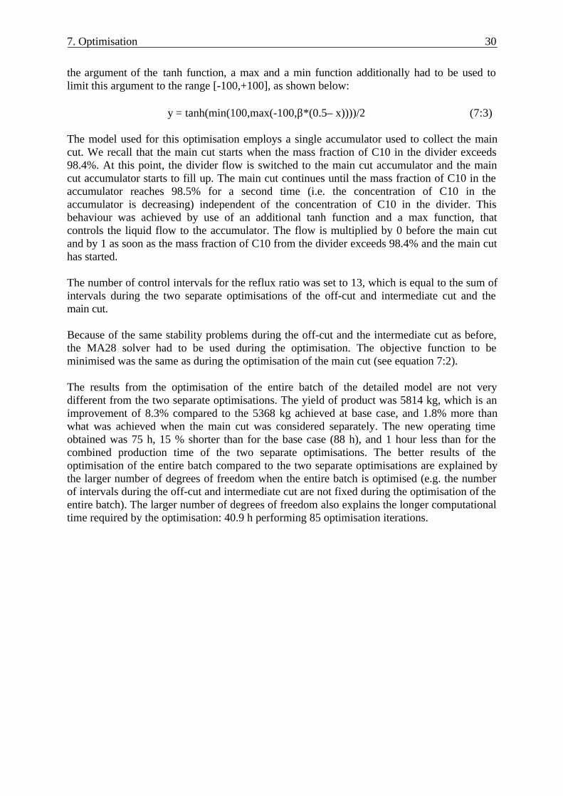
The resulting profile of divider mass fraction and reflux ratio at the optimum are shown infigure 7.3.
Figure 7.3 Reflux ratio and divider mass fraction profiles at optimum for the entire batch.
Off-cut
+
Main Cut
C10C2C4
IntermediateCut
Reflux Ratio
7. Optimisation 32
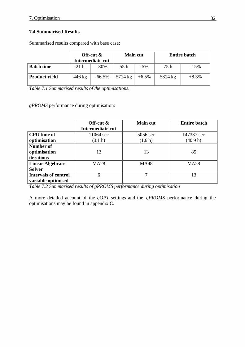
7.4 Summarised Results
Summarised results compared with base case:
Off-cut &Intermediate cut
Main cut Entire batch
Batch time 21 h -30% 55 h -5% 75 h -15%
Product yield 446 kg -66.5% 5714 kg +6.5% 5814 kg +8.3%
Table 7.1 Summarised results of the optimisations.
gPROMS performance during optimisation:
Off-cut &Intermediate cut
Main cut Entire batch
CPU time ofoptimisation
11064 sec(3.1 h)
5056 sec(1.6 h)
147337 sec(40.9 h)
Number ofoptimisationiterations
13 13 85
Linear AlgebraicSolver
MA28 MA48 MA28
Intervals of controlvariable optimised
6 7 13
Table 7.2 Summarised results of gPROMS performance during optimisation
A more detailed account of the gOPT settings and the gPROMS performance during theoptimisations may be found in appendix C.
8. Periodic Operation 33
8. Periodic Operation
In practical operation, the contents of the accumulator used during the intermediate cut aremixed with the fresh feed for the next distillation batch and is then charged to the reboilerdrum (see figure 2.1). This implies that the composition and amount of mixture obtainedduring the intermediate cut will influence the next batch run and its operating procedure. Totake this effect into account, a periodic optimisation has to be performed considering thewhole operating procedure as well as the set up time between every batch run.
8.1 Optimisation with a Multiplexer
For the optimisation of the periodic operation, a separate accumulator is needed for each cut.This can be achieved by using a multiplexer. The multiplexer determines the flow received bythe accumulator for each of the three different cuts according to the following formulae:
Accumulator 1 : Liquid stream from divider*(Acc-2)*(Acc-3)/2Accumulator 2 : Liquid stream from divider*(Acc-1)*(Acc-3)/(-1)Accumulator 3 : Liquid stream from divider*(Acc-2)*(Acc-1)/2
The multiplexer adjusts the value of the control variable Acc. During the off-cut, Acc is keptat the value 1; it can be verified that, in this case, only accumulator 1 receives a non-zero flowfrom the divider. When the intermediate cut starts, the value of Acc is set to 2, and liquid onlyflows into accumulator 2. Finally, during the main cut Acc has the value of 3 and all productwill be gathered in accumulator 3. The values of Acc are set in the gOPT-file used foroptimisation, which means that the number of intervals during each cut has to be fixed withthis method.
The use of a multiplexer also provides an alternative way of switching from the intermediatecut to the main cut. The constraint that the mass fraction of C10 has to exceed 98.4% in thedivider at the start of the main cut can be imposed as an interior point constraint at thebeginning of the first interval of the main cut in the gOPT-file instead of using a tanh function(cf. section 7.3).
Except for using three accumulators instead of only one, exactly the same constraints, numberof intervals and initial conditions as before were used for the optimisation using themultiplexer. The objective function of the optimisation and the switching criterion were alsothe same.
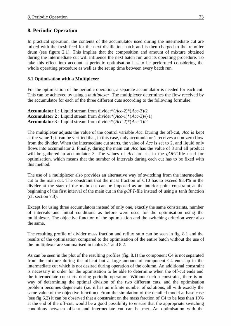
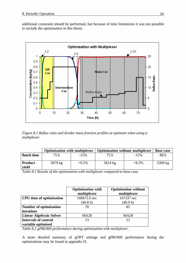
The resulting profile of divider mass fraction and reflux ratio can be seen in fig. 8.1 and theresults of the optimisation compared to the optimisation of the entire batch without the use ofthe multiplexer are summarised in tables 8.1 and 8.2.
As can be seen in the plot of the resulting profiles (fig. 8.1) the component C4 is not separatedfrom the mixture during the off-cut but a large amount of component C4 ends up in theintermediate cut which is not desired during operation of the column. An additional constraintis necessary in order for the optimisation to be able to determine when the off-cut ends andthe intermediate cut starts during periodic operation. Without such a constraint, there is noway of determining the optimal division of the two different cuts, and the optimisationproblem becomes degenerate (i.e. it has an infinite number of solutions, all with exactly thesame value of the objective function). From the simulation of the detailed model at base case(see fig 6.2) it can be observed that a constraint on the mass fraction of C4 to be less than 10%at the end of the off-cut, would be a good possibility to ensure that the appropriate switchingconditions between off-cut and intermediate cut can be met. An optimisation with the
8. Periodic Operation 34
additional constraint should be performed, but because of time limitations it was not possibleto include the optimisation in this thesis.
Figure 8.1 Reflux ratio and divider mass fraction profiles at optimum when using amultiplexer.
Optimisation with multiplexer Optimisation without multiplexer Base caseBatch time 75 h -15% 75 h -15% 88 h
Productyield
5879 kg +9.5% 5814 kg +8.3% 5368 kg
Table 8.1 Results of the optimisation with multiplexer compared to base case.
Optimisation withmultiplexer
Optimisation withoutmultiplexer
CPU time of optimisation 168472.6 sec(46.8 h)
147337 sec(40.9 h)
Number of optimisationiterations
78 85
Linear Algebraic Solver MA28 MA28Intervals of controlvariable optimised
13 13
Table 8.2 gPROMS performance during optimisation with multiplexer.
A more detailed summary of gOPT settings and gPROMS performance during theoptimisations may be found in appendix D.
Off-Cut
IntermediateCut
Main Cut
Reflux Ratio
C10C2C4
8. Periodic Operation 35
8.2 Optimisation of Periodic Operation
For the optimisation of periodic operation, new variables and parameters had to be introducedinto the model. The holdup and the composition of the mixture in the reboiler at the beginningof every batch run was calculated as the mixture obtained by combining fresh feed with thecontents of the intermediate cut accumulator at the end of the batch.
In order to perform a periodic optimisation the following additional equations wereintroduced into the accumulator model of the intermediate cut:
*)()( III MtMtM −=∆ (8:1)
)()()( *,,, txtxtx iIiIiI −=∆ (8:2)
Both MI* and xI,i
* are time-invariant parameters to be determined by the optimisation. Theyrepresent the amount of material and the mass fractions in the intermediate cut accumulator atthe end of the batch. This interpretation can be implemented by enforcing the end-pointconstraint:
ε≤∆+∆ ∑=
10
1,
2 )()(i
fiIfI txtM (8:3)
which practically ensures that, at the final time tf, *)( IfI MtM ≈ and *)( IifI xtix ≈ . Although
theroretically ε should be set to 0, in practice a value of 10-6 was used to avoid an excessivenumber of optimisation iterations.
The material in the intermediate cut is recycled to the reboiler where it is mixed with the freshfeed. To account for this fact, the following variables and equations were introduced into thereboiler model:
BIFB MMMM −+=∆ **
iBIF
iIIiFFiB x
MM
xMxMx ,*
*,
*,*
, −+
⋅+⋅=∆
where MF and xF,i represent the amount and composition of the fresh feed respectively, whileMB and xB,i are the corresponding quantities for the combined feed. This allows us to imposethe following initial conditions at the start of the optimisation:
0)0(* =∆ BM
0)0(*, =∆ iBx
which is equivalent to enforcing the desirable mixing constraints:
*)0( IFB MMM +=
*,
*,,
* )0()( iIIiFFiBIF xMxMxMM ⋅+⋅=+
8. Periodic Operation 36
As the light off-cut is not included explicitly in the model, its influence is approximated bythe use of constants, λi:
( ) ( ) ( )00 ,*,,
*, iBiiIiFiB MMMM −⋅+=∆ λ
where λi is the fraction of component i removed during the light off-cut.
The objective function to be optimised was:
Profit
++=
−cutofflightsetupprod
C
tttM
_
10 (8:4)
where tsetup is approximated to 7 hours. tlight_off-cut was set to 7 hours as during the simulation.
An optimisation was performed with fixed amount and composition of the fresh feed. Thisoptimisation resulted in a shorter production time, but less product was produced compared tothe base case. The result is explained by the fact that the fresh feed was fixed during theoptimisation. When the intermediate cut is optimised, the total feed charge will be less thanbefore, because of less amount of mixture in the accumulator of the intermediate cut. Thisfurther means that less product will be obtained at the end of the next batch run. As aconsequence the amount of product obtained during the intermediate cut will not be madesmaller by the optimiser. Instead, only the time of production is decreased to maximise theobjective function. However when the production time is decreased the yield of productduring the main cut is not as large at the end of the operation as if the production time wouldbe allowed to be longer, and this explains why the product yield obtained is actually less thanduring the base case. An easy way of getting around the problem is to optimise the amount offresh feed as well. Thus an optimisation with the amount of fresh feed as an additional timeinvariant parameter was performed.
Optimisation of periodic operationwith fresh feed as fixed parameter
Base Case
Batch time 69 h -22% 88 h
Product yield 5057 kg -5.8% 5368 kg
Table 8.3 Results of optimisation of the periodic operation compared to base case.
8.3 Optimisation with Fresh Feed as Time Invariant Parameter
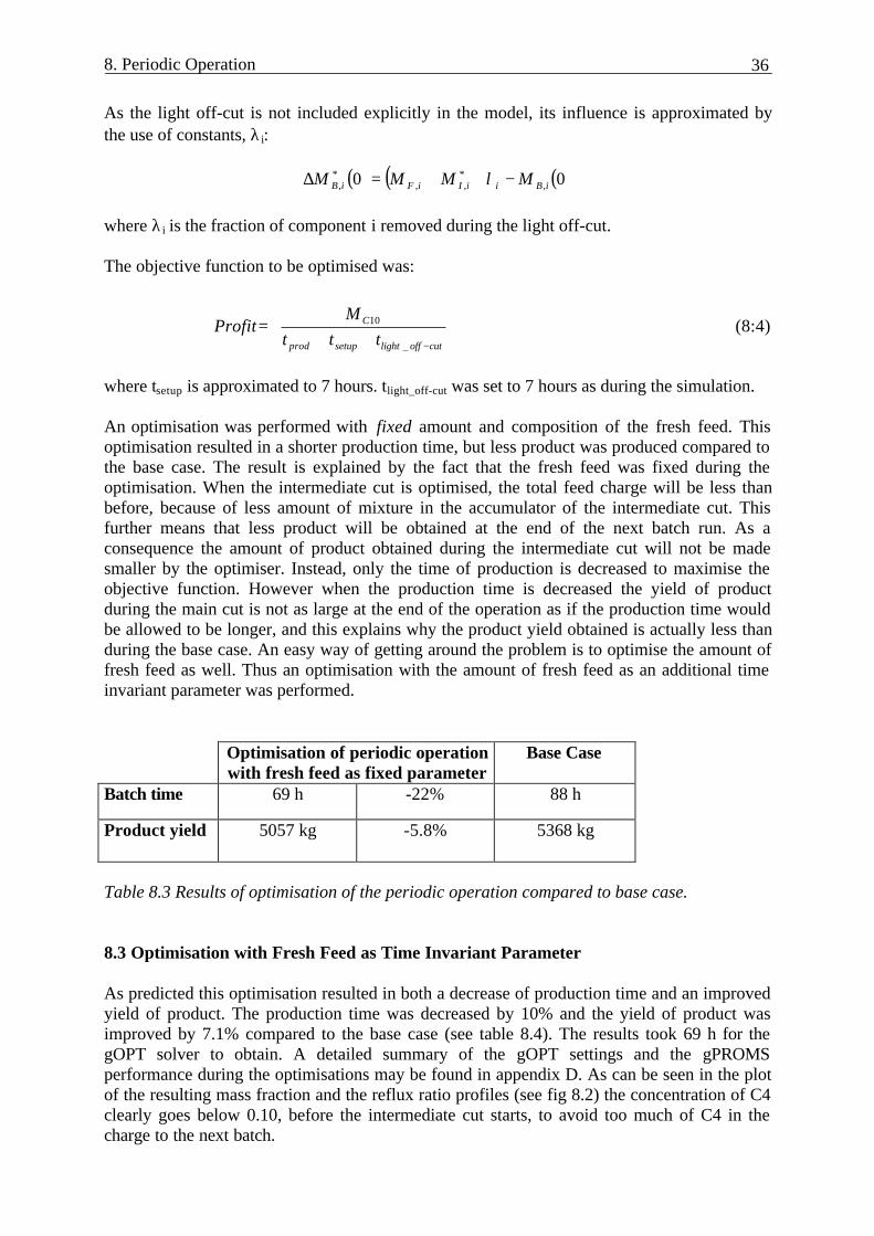
As predicted this optimisation resulted in both a decrease of production time and an improvedyield of product. The production time was decreased by 10% and the yield of product wasimproved by 7.1% compared to the base case (see table 8.4). The results took 69 h for thegOPT solver to obtain. A detailed summary of the gOPT settings and the gPROMSperformance during the optimisations may be found in appendix D. As can be seen in the plotof the resulting mass fraction and the reflux ratio profiles (see fig 8.2) the concentration of C4clearly goes below 0.10, before the intermediate cut starts, to avoid too much of C4 in thecharge to the next batch.
8. Periodic Operation 37
Figure 8.2 Reflux ratio and divider mass fraction profiles at optimum of the periodicoperation.
Optimisation of periodic operationwith fresh feed as time invariant parameter
Base Case
Batch time 79 h -10% 88 h
Product yield 5751 kg +7.1% 5368 kg
Table 8.4 Results of optimisation of the periodic operation compared to base case.
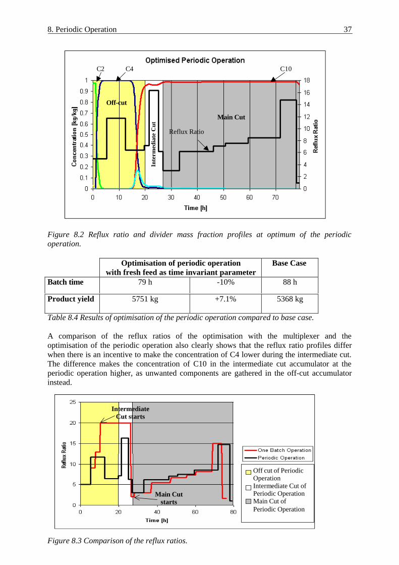
A comparison of the reflux ratios of the optimisation with the multiplexer and theoptimisation of the periodic operation also clearly shows that the reflux ratio profiles differwhen there is an incentive to make the concentration of C4 lower during the intermediate cut.The difference makes the concentration of C10 in the intermediate cut accumulator at theperiodic operation higher, as unwanted components are gathered in the off-cut accumulatorinstead.
Figure 8.3 Comparison of the reflux ratios.
Off-cut
Main Cut
Inte
rmed
iate
Cut
Reflux Ratio
C10C2 C4
IntermediateCut starts
Off cut of PeriodicOperation Intermediate Cut ofPeriodic Operation
Main Cut ofPeriodic Operation
Main Cutstarts
9. Conclusions and Directions for Future Work 38
9. Conclusions and Directions for Future Work
9.1 Conclusions
The optimisation of the batch process shows that it is possible to reduce the time ofproduction while simultaneously increasing the product yield, just by modifying the timevariation of the reflux ratio. More specifically, results obtained from the performedoptimisation of the model of the batch process were:
• 15% less time of production
• 9% higher product yield.
The optimisation took about 41 h of computation to perform on a SGI Origin 2000.
A new procedure of the reflux ratio could easily be realised in the plant without any additionalinvestment costs and would result in a noticeable increase of profit.
However, as the actual process is operated periodically, the amount of product at the end ofthe operation is not the only factor that affects the profit. The mixture obtained during theintermediate cut that is mixed with the fresh feed also influences the production. This wasaccounted for when performing the optimisation of the periodic operation. The results fromthis optimisation were:
• 10.5% less time of production
• 7.9% higher product yield
The duration of the optimisation this time was about 69 h.
The results were obtained when the amount of fresh feed was considered as a degree offreedom for optimisation. If the fresh feed is set as a fixed parameter, i.e. not optimised duringthe whole periodic operation, the amount of product obtained will as a matter of fact be lessthan at base case.
An important conclusion to make regarding the performance of gPROMS is that it is possibleto use gPROMS to optimise a detailed model of a batch distillation column within acceptabletimes of optimisation. However a very fast computer is needed, like for example a SGI Origin2000 used in this work. The default solver in version 1.7 of gPROMS, MA48 was observed tonot be as stable as the MA28 solver, which therefore was used in most cases, even though itrequires slightly more computational time.
9.2 Directions for Future Work
In the immediate future the optimisation of the entire batch with the multiplexer formulation,including the additional constraint at the end of the off-cut, should be performed to make surethat reliable results are obtained.
9. Conclusions and Directions for Future Work 39
The optimisation could include even more intervals, or the optimisation could be performedwith just the number of intervals and a bound for the allowed time horizon of the wholeoperation time set, instead of fixing the number of intervals for each cut.
The model could be made even more detailed, for example by using tray efficiencies that varyover time. The time to simulate the model would then of course increase and it would be evenmore important to find a way to make the simulation of the model faster. One option could beto include equations used by the foreign object IKCAPE directly in the model. The solver ofgPROMS would then work more effectively. A shorter simulation time would also make itpossible to optimise the whole operation, including the light component off-cut and the heavycomponent off-cut making the optimisation results of the periodic operation more reliable.
The actual composition of the feed charged during one batch distillation can not be knownprecisely, as the composition of the fresh feed arriving from upstream units varies due tovariations in process conditions. However the feed composition has shown to influence theoperation procedure in a great extent (Gautheron [12]), thus optimisations with different feedcompositions should be performed. This shows two potential areas for future work. First theoptimisation of process operation under uncertainty due to the uncertain composition of thefresh feed, and secondly on-line optimisation to account for this uncertainty by improvingoperating conditions during the actual operation of each batch. However, the latter optionrequires a numerically tolerant model and very fast computing times during optimisation.
Finally, as already mentioned, the production is also performed with a packed column insteadof a tray column. This batch process could also be optimised in gPROMS using the already, inSPEEDUP, developed model (see Gautheron [12]).
Nomenclature 40
Nomenclature
A Antoine’s coefficientArea cross sectional area m2
B Antoine’s coefficientbias steady state control valueC Antoine’s coefficientCp heat capacity kJ/(kmol.K)Error set point and variable errorƒ fugacityFfak vapour load (F-factor) m/s.(kg/m3)0.5
g acceleration due to gravity m/s2
gain controller gainh specific enthalpy kJ/kmol∆H°298 latent heat of vaporisation kJ/kmol∆HV298 heat of vaporisation kJ/kmolheight liquid level in reflux drum mhf liquid level on tray mhweir weir height mh’weir height of liquid above weir mIerror integral errorIin input signalk equilibrium coefficientk’ heat transfer coefficient W/m2.Kkliq liquid flow coefficient kmol.m2/3/hL liquid flowrate kmol/hLevel liquid level in reboiler m/mlw weir length mM molar holdup kmolMW molecular weight kmol/kgNC number of componentsP pressure barp° vapour pressure of pure component Pa∆P pressure drop mbar∆Ptr dry pressure drop mbarQ rate of heat transfer WR reflux ratioreset reset time of PI-controllerSp set point of PI-controllerT temperature °CU internal energy kJv molar volume m3/kmolVdowncomer volume of downcomer m3
vf liquid load m3/(m2.h)value calculated value of PI-controllerVges volume reboiler m3
W mass holdup kgwg vapour velocity m/sx liquid composition kmol/kmolxM liquid composition kg/kgy vapour composition kmol/kmol
Nomenclature 41
Greek Letters
εl liquid fractionΦ fugacity coefficientγ activity coefficientη tray efficiencyλ constantµ parameter of control variableρ density kg/m3
Subscripts
B batchC condenserF feedI intermediate cuti componentin inletk trayout outletR reboiler drumcrit critical point
Superscripts
L liquidV vapour* ideal composition
References 42
References
[1] Barolo, M. and Fabrizio Berto, “Composition Control on Batch Distillation: Binary andMulticomponents Mixtures”, Ind. Eng. Chem. Res., 37, 4689 (1998).
[2] Barolo, M. and F. Botteon, “Simple Method of Obtaining Pure Products by BatchDistillation”, AIChE J., 43, 2601 (1997).
[3] Barolo, M., G.B. Guarise, N. Ribson, S. Rienzi, A. Trotta and S. Macchietto, “SomeIssues in the Design and Operation of a Batch Distillation Column with a MiddleVessel”, Comput. Chem. Eng. , S20, S37 (1996).
[4] Bosley, J.R. and Thomas F. Edgar, “An efficient dynamic model for batch distillation”,J. Proc. Cont., 4, 195 (1994).
[5] Carlsson, E.C., “Don’t Gamble With Physical Properties For Simulations”, Chem. Eng.Progress (Oct 1996).
[6] Diwekar, U.M., “How Simple Can it be ? – A Look at the Models for BatchDistillation”, Comput. chem. Engng., 18, S451 (1994).
[7] Diwekar, U.M., “Unified Approach to Solving Optimal Design Control Problems inBatch Distillation”, AIChE J., 38, 1551 (1992).
[8] Diwekar, U.M., R.K. Malik and K. P. Madhavan, “Optimal Reflux Rate PolicyDetermination For Multicomponent Batch Distillation Columns”, Comput. Chem.Engng., 11, 629 (1987).
[9] Furlonge, H.I., “Optimal Operation of Unconventional Batch Distillation Columns”,PhD Thesis, University of London, January 2000.
[10] Furlonge, H.I., C.C. Pantelides and E. Sørensen, “Optimal Operation of MultivesselBatch Distillation Columns”, AIChE J., 45, 781 (1999).
[11] Galindez, H. and AA Fredenslund, “Simulation of Multicomponent Batch DistillationProcesses”, Comput. Chem. Engng., 12, 281 (1988).
[12] Gautheron, S., “Modellierung und Optimierung von Batchdestillationskolonnen”,Diplomarbeit, Bayer AG Leverkusen (1999).
[13] Kooijman, H.A. and R. Taylor, “A Non-Equilibrium Model For Dynamic Simulation ofTray Distillation Columns”, AIChE J., 41, 1852 (1995).
[14] Li, P., “Entwicklung optimaler Führungsstrategien für Batch-Destillationsprocesse”,Doktorarbeit, Bayer AG Leverkusen (1998).
[15] Logsdon, J.S. and L.T. Biegler, “Accurate solution of differential-algebraic optimizationproblems”, Ind. Eng. Chem., 28, 1628-1639 (1989).
[16] Nilsson, B., “Föreläsningsanteckningar: Process Simulering”, Lund Institute ofTechnology, Lund (1999).
References 43
[17] Oh, M., “Modelling and Simulation of Combined Lumped and Distributed Processes”,PhD Thesis, University of London (1995).
[18] Pantelides, C.C, “Dynamic Behaviour of Process Systems”, Lecture Notes, Centre forProcess Systems Engineering, Imperial College of Science, Technology and Medicine,London (1998).
[19] Perry, R.H. and D. Green, “Perry’s Chemical Engineers’ Handbook, McGraw Hill BookCompany, Inc New York, 6th ed., 1984.
[20] Process Systems Enterprise Ltd., gPROMS Advanced User Guide, London (1999).
[21] Process Systems Enterprise Ltd., gPROMS Introductory User Guide, London (1999).
[22] Sadotomo, H. and K. Miyahara, “Calculation procedure for multicomponent batchdistillation”, Int. Chem. Engng., 23, 56 (1983).
[23] Skogestad, S., B. Wittgens, E. Sørensen, and R. Litto, “Multivessel Batch Distillation”,AIChE J., 43, 971 (1997).
[24] Vassiliadis, V.S., R.W.H. Sargent, and C.C. Pantelides, “Solution of a Class ofMultistage Dynamic Optimisation Problems: 1. Problems without Path Constraints”,Ind. Eng. Chem. Res., 33, 2111 (1994a).
[25] Vassiliadis, V.S., R.W.H. Sargent, and C.C. Pantelides, “Solution of a Class ofMultistage Dynamic Optimisation Problems: 2. Problems with Path Constraints”, Ind.Eng. Chem. Res., 33, 2123 (1994b).
Appendix A 44
Appendix A
Feed Composition
C1 0,03C2 0,08C3 0,02C4 9,45C5 0,11C6 0,06C7 0,03C8 0,03C9 0,07C10 66,05C11 0,70C12 1,35C13 0,31C14 0,02C15 0,03C16 0,86C17 0,07C18 0,12C19 0,10C20 15,69C21 0,23C22 0,94C23 0,08C24 0,03C25 0,03C26 0,05C27 0,01C28 0,09C29 3,14C30 0,22
Figure A.1 GC analysis of the feed composition
ReboilerReboiler
C1 is the light component and C30is the heavy component.
Appendix B 45
Appendix B
The Equations of the Model
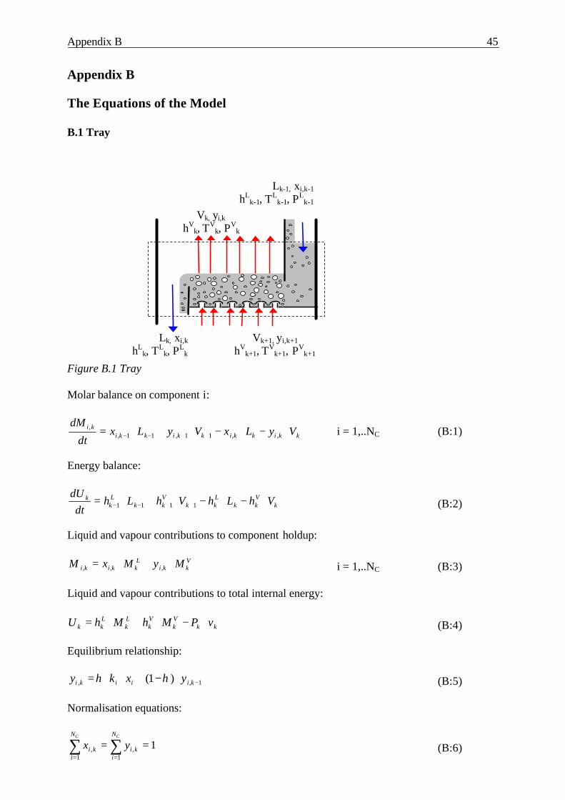
B.1 Tray
Figure B.1 Tray
Molar balance on component i:
kkikkikkikkiki VyLxVyLx
dt
dM⋅−⋅−⋅+⋅= ++−− ,,11,11,
, i = 1,..NC (B:1)
Energy balance:
kVkk
Lkk
Vkk
Lk
k VhLhVhLhdt
dU⋅−⋅−⋅+⋅= ++−− 1111 (B:2)
Liquid and vapour contributions to component holdup:
Vkki
Lkkiki MyMxM ⋅+⋅= ,,, i = 1,..NC (B:3)
Liquid and vapour contributions to total internal energy:
kkVk
Vk
Lk
Lkk vPMhMhU ⋅−⋅+⋅= (B:4)
Equilibrium relationship:
1,, )1( −⋅−+⋅⋅= kiiiki yxky ηη (B:5)
Normalisation equations:
∑ ∑= =
==C CN
i
N
ikiki yx
1 1,, 1 (B:6)
Lk-1, xi,k-1
hLk-1, TL
k-1, PLk-1
Vk, yi,k
hVk, TV
k, PVk
Lk, xi,k
hLk, TL
k, PLk
Vk+1, yi,k+1
hVk+1, TV
k+1, PVk+1
Appendix B 46
Ideal mixing:
1,, −= kiki xx (B:7)
Liquid holdup on the tray:
liq
liqdowncomerlweirLk MW
VhAreaM
ρε ⋅+⋅⋅=
)( '
(B:8)
Weir formula:
( ) ( )
23/2
3/1'
1
2.0
2/45.1
−
⋅−⋅
−⋅⋅+
⋅+=
l
vapFak
vapliql
wweirweir
F
gclL
ghh
ε
ρ
ρρε (B:9)
Liquid and vapour load:
liqkliqwf MWLlv ⋅⋅=⋅⋅ 10ρ (B:10)
2/1vapgFak wF ρ⋅= (B:11)
vapkvapg MWVAreaw ⋅=⋅⋅ +1ρ (B:12)
Pressure drop across tray:
trliqf PghP ∆+⋅⋅=∆ ρ (B:13)
( )Faktr FfP =∆ (B:14)
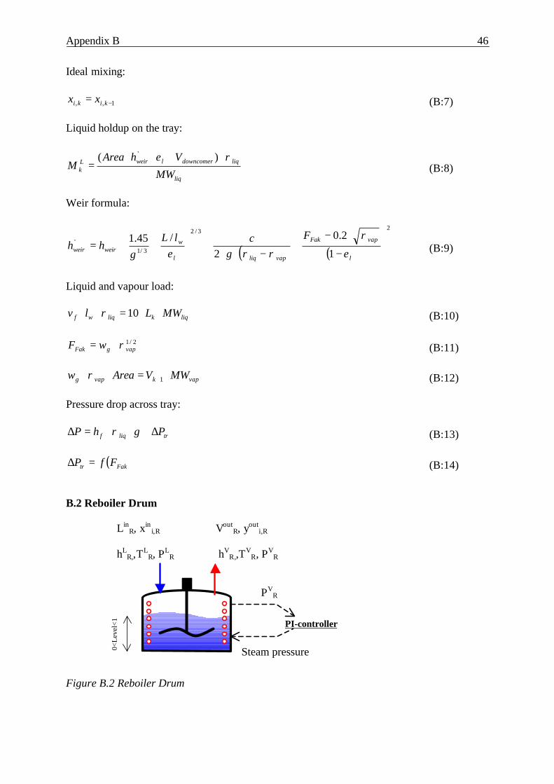
B.2 Reboiler Drum
Figure B.2 Reboiler Drum
PI-controller
PVR
Steam pressure
LinR, xin
i,R
hLR,,TL
R, PLR
VoutR, yout
i,R
hVR,,TV
R, PVR
0<L
evel
<1
Appendix B 47
Molar balance on component i:
outR
outRi
inR
inRi
Ri VyLxdt
dM⋅−⋅= ,´,
, i = 1,..NC (B:15)
Energy balance:
Rout
RVR
inR
inR
R QVhLhdt
dU+⋅−⋅= (B:16)
Liquid and vapour contributions to component holdup:
VR
outRi
LRRiRi MyMxM ⋅+⋅= ,,, i = 1,..NC (B:17)
Equilibrium relationship:
iii xky ⋅= (B:18)
Normalisation equation:
∑ = 1iy (B:19)
Liquid holdup:
liqliqges MWMVLevel ⋅=⋅⋅ ρ (B:20)
Heat conduction:
( ) ( )liqsteambottompipepipe TTALevelAkHeat −⋅+⋅⋅⋅= ,'001.0 (B:21)
( ) bureSteampressaTsteam +⋅= log (B:22)where a and b are constants.
B.3 PI-controller
inISpError −= (B:23)
( )Error
dtId error = (B:24)
+⋅+=resetI
Errorgainbiasvalue error (B:25)
Appendix B 48
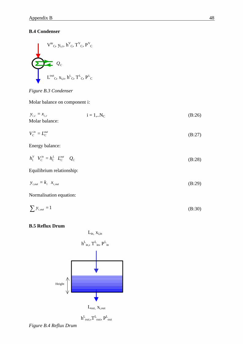
B.4 Condenser
Figure B.3 Condenser
Molar balance on component i:
cici xy ,, = i = 1,..NC (B:26)Molar balance:
outC
inC LV = (B:27)
Energy balance:
CoutC
LC
inC
V QLhVh +⋅=⋅1 (B:28)
Equilibrium relationship:
outiiouti xky ,, ⋅= (B:29)
Normalisation equation:
∑ = 1,outiy (B:30)
B.5 Reflux Drum
Figure B.4 Reflux Drum
CQ
VinC, yi,c, hV
C, TVC, PV
C
LoutC, xi,c, hL
C, TLC, PL
C
Lin, xi,in
hLin,, TL
in, PLin
Lout, xi,out
hLout,,TL
out, PLout
Height
Appendix B 49
Molar balance on component i:
outoutiininiki LxLx
dt
dM⋅−⋅= ,,
, i = 1,..NC (B:31)
Energy balance:
outLoutin
Lin LhLh
dt
dU⋅−⋅= (B:32)
Liquid holdup:
5.1heightkL liqout ⋅= (B:33)
HeightAreaMWM liqliq ⋅⋅=⋅ ρ (B:34)
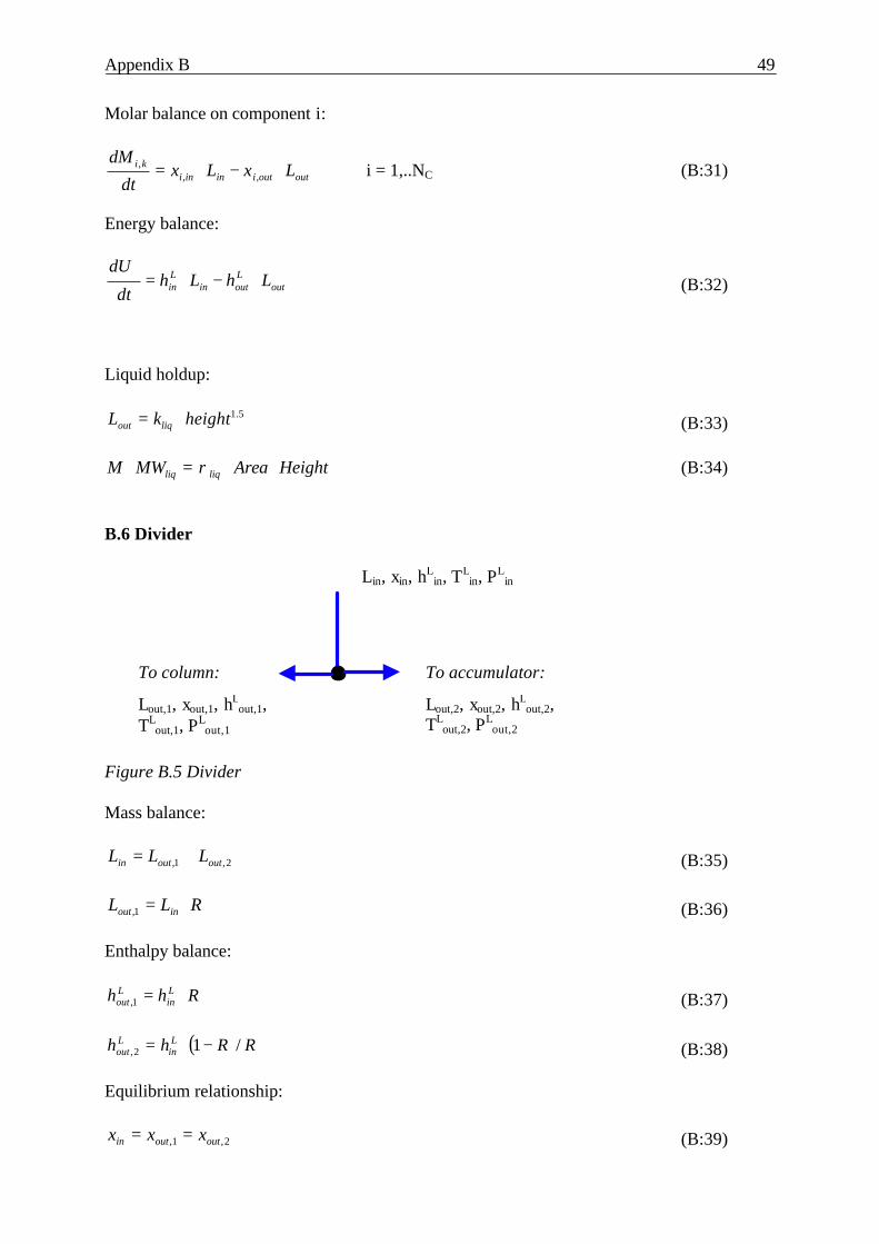
B.6 Divider
Figure B.5 Divider
Mass balance:
2,1, outoutin LLL += (B:35)
RLL inout ⋅=1, (B:36)
Enthalpy balance:
Rhh Lin
Lout ⋅=1, (B:37)
( ) RRhh Lin
Lout /12, −⋅= (B:38)
Equilibrium relationship:
2,1, outoutin xxx == (B:39)
Lin, xin, hLin, TL
in, PLin
Lout,1, xout,1, hLout,1,
TLout,1, PL
out,1
To column:
Lout,2, xout,2, hLout,2,
TLout,2, PL
out,2
To accumulator:
Appendix B 50
Pressure:
Lout
Lout
Lin PPP 2,1, == (B:40)
Temperature:
Lout
Lout
Lin TTT 2,1, == (B:41)
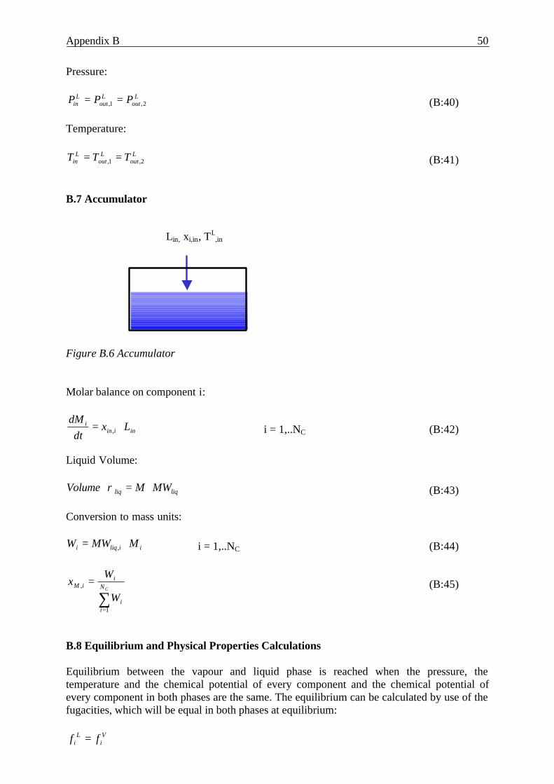
B.7 Accumulator
Figure B.6 Accumulator
Molar balance on component i:
iniini Lx
dtdM
⋅= , i = 1,..NC (B:42)
Liquid Volume:
liqliq MWMVolume ⋅=⋅ ρ (B:43)
Conversion to mass units:
iiliqi MMWW ⋅= , i = 1,..NC (B:44)
∑=
=CN
ii
iiM
W
Wx
1
, (B:45)
B.8 Equilibrium and Physical Properties Calculations
Equilibrium between the vapour and liquid phase is reached when the pressure, thetemperature and the chemical potential of every component and the chemical potential ofevery component in both phases are the same. The equilibrium can be calculated by use of thefugacities, which will be equal in both phases at equilibrium:
Vi
Li ff =
Lin, xi,in, TL,in
Appendix B 51
This leads to:
pyfx iiiii ⋅⋅Φ=⋅⋅ ° *γ
where the following approximations may be made:
• at low pressure: °° = ii pf
• ideal vapour phase: 1=Φ i
• ideal liquid phase: 1=iγ
The separation in most separation columns used in chemical industries are operated at relativelow pressure and the vapour phase can therefore be assumed to be ideal. This leads to theexpression:
ii
i
ii p
pxy
k γ⋅==°*
where the vapour pressure of every pure component, pi° is calculated with the Antoine-
equation:
TCB
Api
iii +
+=°ln
(the parameters Ai, Bi, Ci can be found in literature).
The activity coefficient, γi depends on both the temperature and concentration of thecomponent and can be calculated with NRTL, UNIQUAC or UNIFAC models (Li [14])
Tray efficiency:
A theoretical tray means that vapour leaving the tray is in equilibrium with the liquid leavingthe tray. In practice this never happens and tray efficiencies have to be used:
1,*,
1,,
+
+
−
−=
kiki
kikik yy
yyη
ηk is dependent of the volatility of the component and the efficiency of the mixing. ηk usuallyhas a value between 0.7-1.0 and can easily be evaluated with an experiment. The trayefficiencies in this work have been assumed to be equal for all the components, although thisis in reality only true for binary systems (Kooijman and Taylor [13]).
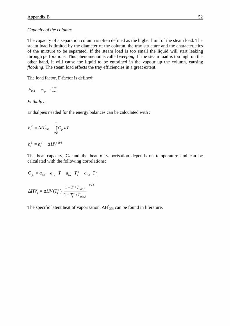
Appendix B 52
Capacity of the column:
The capacity of a separation column is often defined as the higher limit of the steam load. Thesteam load is limited by the diameter of the column, the tray structure and the characteristicsof the mixture to be separated. If the steam load is too small the liquid will start leakingthrough perforations. This phenomenon is called weeping. If the steam load is too high on theother hand, it will cause the liquid to be entrained in the vapour up the column, causingflooding. The steam load effects the tray efficiencies in a great extent.
The load factor, F-factor is defined:
2/1vapgFak wF ρ⋅=
Enthalpy:
Enthalpies needed for the energy balances can be calculated with :
∫+∆= °T
pVi dTCHh
i
298298
298i
Vi
Li HVhh ∆−=
The heat capacity, Cp and the heat of vaporisation depends on temperature and can becalculated with the following correlations:
33,
22,1,0, jijiiip TaTaTaaC
i⋅+⋅+⋅+=
38.0
,
,
/1
/1)(
−
−∆=∆
icritv
i
icritvii TT
TTTHVHV
The specific latent heat of vaporisation, ∆H°298 can be found in literature.
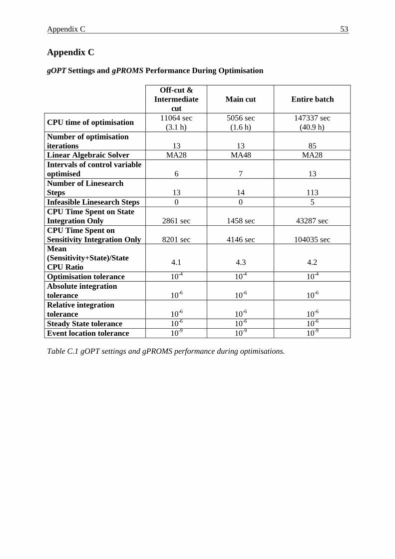
Appendix C 53
Appendix C
gOPT Settings and gPROMS Performance During Optimisation
Off-cut &Intermediate
cutMain cut Entire batch
CPU time of optimisation 11064 sec(3.1 h)
5056 sec(1.6 h)
147337 sec(40.9 h)
Number of optimisationiterations 13 13 85Linear Algebraic Solver MA28 MA48 MA28Intervals of control variableoptimised 6 7 13Number of LinesearchSteps 13 14 113Infeasible Linesearch Steps 0 0 5CPU Time Spent on StateIntegration Only 2861 sec 1458 sec 43287 secCPU Time Spent onSensitivity Integration Only 8201 sec 4146 sec 104035 secMean(Sensitivity+State)/StateCPU Ratio 4.1 4.3 4.2
Optimisation tolerance 10-4 10-4 10-4
Absolute integrationtolerance 10-6 10-6 10-6
Relative integrationtolerance 10-6 10-6 10-6
Steady State tolerance 10-6 10-6 10-6
Event location tolerance 10-9 10-9 10-9
Table C.1 gOPT settings and gPROMS performance during optimisations.
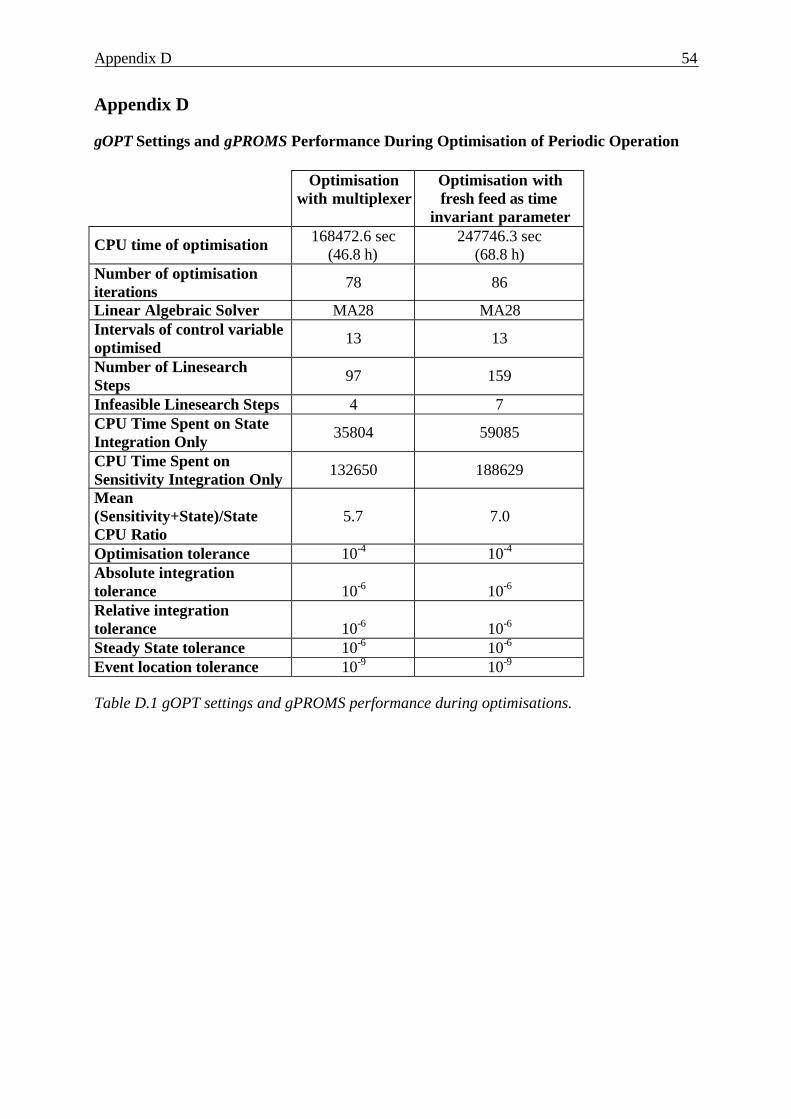
Appendix D 54
Appendix D
gOPT Settings and gPROMS Performance During Optimisation of Periodic Operation
Optimisationwith multiplexer
Optimisation withfresh feed as time
invariant parameter
CPU time of optimisation 168472.6 sec(46.8 h)
247746.3 sec(68.8 h)
Number of optimisationiterations 78 86
Linear Algebraic Solver MA28 MA28Intervals of control variableoptimised 13 13
Number of LinesearchSteps 97 159
Infeasible Linesearch Steps 4 7CPU Time Spent on StateIntegration Only 35804 59085
CPU Time Spent onSensitivity Integration Only 132650 188629
Mean(Sensitivity+State)/StateCPU Ratio
5.7 7.0
Optimisation tolerance 10-4 10-4
Absolute integrationtolerance 10-6 10-6
Relative integrationtolerance 10-6 10-6
Steady State tolerance 10-6 10-6
Event location tolerance 10-9 10-9
Table D.1 gOPT settings and gPROMS performance during optimisations.