modelling approaches for predictive control of large-scale

IRI-TR-01-09

Modelling Approaches for Predictive

Control of Large-Scale Sewage Systems

Carlos Ocampo-MartinezVicenc Puig∗

cetto

Text Box

09-01

Abstract

In this report, model predictive control (MPC) of large-scale sewage systems is addressed consid-ering different modelling approaches that include several inherent continuous/discrete phenom-ena (overflows in sewers and tanks) and elements (weirs) in the system that result in distinctbehaviour depending on the dynamic state (flow/volume) of the network. These behaviourscan not be neglected nor can be modelled by a pure linear representation. In order the MPCcontroller takes into account these phenomena and elements, a modelling approach based onpiece-wise linear functions is proposed and compared against a hybrid modelling approach pre-viously reported by the authors. Control performance results and associated computation timesof the closed-loop scheme considering both modelling approaches are compared by using a realcase study based on the Barcelona sewer network.

∗ Vicenc Puig is with the Control Department (ESAII), Technical University of Catalonia (UPC),Rambla de Sant Nebridi, 10, 08222 Terrassa, Spain, e-mail: [email protected]

Institut de Robotica i Informatica Industrial (IRI)Consejo Superior de Investigaciones Cientıficas (CSIC)

Universitat Politecnica de Catalunya (UPC)Llorens i Artigas 4-6, 08028, Barcelona, Spain

Tel (fax): +34 93 401 5750 (5751)

http://www.iri.upc.edu

Corresponding author:

C. Ocampo-Martineztel: +34 93 401 5786

[email protected]

http://www.iri.upc.edu/people/cocampo

c© Copyright IRI, 2009

Section 1 Introduction 1

1 Introduction

Sewer networks are considered as complex large-scale systems since they are geographicallydistributed and decentralized with a hierarchical structure. Each sub-system is in itself composedof a large number of elements with time-varying behavior, exhibiting numerous operating modesand subject to changes due to external conditions (weather) and operational constraints.

Most cities around the world have sewage systems that combine sanitary and storm waterflows within the same network. This is why these networks are known as Combined SewageSystems (CSS). During rain storms, wastewater flows can easily overload these CSS, therebycausing operators to dump the excess water into the nearest receiver environment (rivers, streamsor sea). This discharge to the environment, known as Combined Sewage Overflow (CSO),contains biological and chemical contaminants creating a major environmental and public healthhazard. Environmental protection agencies have started forcing municipalities to find solutions inorder to avoid those CSO events. A possible solution to the CSO problem would be to enhanceexisting sewer infrastructure by increasing the capacity of the wastewater treatment plants(WWTP) and by building new underground retention tanks. But in order to take profit of theseexpensive infrastructures, it is also necessary a highly sophisticated real-time control (RTC)scheme which ensures that high performance can be achieved and maintained under adversemeteorological conditions [27]. The advantage of RTC applied to sewer networks has beendemonstrated by an important number of researchers during the last decades, see [10, 23, 22, 14].Comprehensive reviews that include a discussion of some existing implementations are given by[25] and cited references therein, while practical issues are discussed by [26], among others.

The RTC scheme in sewage systems might be local or global. When local control is applied,flow regulation devices use only measurements taken at their specific locations. While thiscontrol structure is applicable in many simple cases, in a big city, with a strongly interconnectedsewer network and a complex infrastructure of sensors and actuators, it may not be the mostefficient alternative. Conversely, a global control strategy, which computes control actions takinginto account real-time measurements all through the network, is likely the best way to use theinfrastructure capacity and all the available sensor information. Global RTC deals with theproblem of generating control strategies for the control elements in a sewer network, ahead oftime, based on a predictive dynamic model of the system, and readings of the telemetry system,in order to avoid street flooding, prevent CSO discharges to the environment, minimize thepollution, homogenise the utilization of sewage system storage capacity and, in most of cases,minimize the operating costs [27, 9, 32, 28]. The multivariable and large-scale nature of sewernetworks have lead to the use of some variants of Model Predictive Control (MPC), as globalcontrol strategies [10, 23, 22, 14]. The MPC strategy, also referred as Receding Horizon Control(RHC) or Moving Horizon Optimal Control (MHOC), is one of the few advanced methodologieswhich has significant impact on industrial control engineering. MPC is being applied in processindustry because it can handle multivariable control problems in a natural form, it can take intoaccount actuator limitations and allows constraints consideration.

In order to use MPC within a global RTC scheme of a sewage system, a model able topredict its future states over a prediction horizon taking into account a rain forecast is needed.Sewer networks are systems with complex dynamics since water flows through sewers in openchannel. These flow dynamics are described by Saint-Vennant’s partial differential equationsthat can be used to perform simulation studies but are highly complex to be solved in real time.When developing a control-oriented model, there is always a trade-off between model descriptionaccuracy and computational complexity. As a general rule, the model used for control purposesshould be descriptive enough to capture the most significant dynamics of the system but simpleenough to be scalable for large-scale networks such that real-time implementation is allowed.

Several control-oriented modelling techniques have been presented in the literature that deal

2 Modelling Approaches for MPC of Sewage Systems

with the global RTC of sewage systems, see [14, 8]. In [18, 6], it is used a conceptual linearmodel based on assuming that a set of sewers in a catchment can be considered as a virtualtank. The main reason to use a linear model is to preserve the convexity of the optimizationproblems related to the MPC strategy. A similar approach can be found in an early referenceon MPC applied to sewage systems [10].

However, there exist several inherent phenomena (overflows in sewers and tanks) and ele-ments (weirs) in the system that result in distinct behaviour depending on the state (flow/volume)of the network. These discontinuous behaviours can not be neglected nor can be modelled by apure linear model. Additionally, the presence of intense precipitation causes that new flow pathsappear. Thus, some flow paths are not always present in the sewer network and depend of itsstate and disturbances (rain). According to this observed behaviour, a control-oriented modelmethodology that allows to consider and incorporate overflows and other logical dynamics inmost of the sewer network elements is needed. One of the main contributions of this paperis to describe and analyze these continuous/discrete dynamic behaviours in order to proposea control-oriented modelling approach focused on designing an MPC-based RTC scheme forlarge-scale sewer networks.

First of all, an hybrid modelling approach based on the Mixed Logical Dynamical (MLD)paradigm, introduced in [2] and already used to model hybrid elements in sewer networks willbe briefly presented (see [16] for further details). However, from previous works in this line doneby the authors (see [17]), the inclusion of those discontinuous behaviours in the MPC problemincreases the computation time of the control law. So, some relaxation should be thought inthe modelling approach such that it can be considered within the RTC of large-scale sewernetworks. Therefore, another contribution of this paper consists in proposing an alternativemodelling approach consisting on representing the sewage system by using piece-wise linearfunctions (in the sequel called PWLF-based model or simply PWLF model), following the ideasproposed by Schechter [24]. The aim of this modelling approach is to reduce the complexity of theMPC problem by avoiding the logical variables introduced by the MLD system representation.The idea behind the PWLF modelling approach consists in having a description of the networkusing functions that, despite their discontinuous nature, are considered as quasi-convex [4], andhence the optimization problems associated to the non-linear MPC strategy used for RTC ofthe sewage system. In this way, the resulting optimization problems does not include integervariables what allows saving computation time.

The remainder of the paper is organized as follows. In Section 2, control-oriented modellingof sewer networks is revised and the issue of discontinuous dynamics is presented. Two modellingapproaches for large-scale sewer networks are explained and discussed. RTC scheme for sewagesystems based on MPC strategy is addressed in Section 3 taking into account the modellingapproaches presented in previous section. Section 4 presents a real case study based on theBarcelona sewer network. This case study is used to compare the closed-loop performance whenimplementing a predictive controller based on the modelling approaches presented in Section 2.Section 5 shows and discusses the comparisons of performance and computation times of theclosed-loop system considering the mentioned control-oriented modelling approaches. Finally,main conclusions close the paper in Section 6.

2 RTC-Oriented Modelling of Large-Scale Sewer Networks

2.1 Principles of Mathematical Modelling of Sewage Systems

One of the most important stages on design of RTC schemes for sewer networks, in the caseof using a model-based control technique as MPC, lies on the modelling task. This is becauseperformance of model-based control techniques is very dependant of model quality. So, in order

Section 2 RTC-Oriented Modelling of Large-Scale Sewer Networks 3

to design an MPC-based RTC scheme with an acceptable performance, a system model withaccuracy enough should be used but keeping complexity manageable. This section is focused onthe determination of a control-oriented sewer network model taking into account the trade-offbetween accuracy and complexity and keeping always in mind the RTC inherent restrictions[10].

Water flow in sewer pipes is open-channel, that corresponds to the flow of a certain fluid ina channel in which the fluid shares a free surface with an empty space above. The Saint-Venantequations, based on physical principles of mass conservation and energy, allow the accuratedescription of the open-channel flow in sewer pipes [15] and therefore also allow to have adetailed non-linear description of the system behaviour. These equations are expressed as:

∂qx,t

∂x+

∂Ax,t

∂t= 0, (1)

∂qx,t

∂t+

∂

∂x

(

q2x,t

Ax,t

)

+ gAx,t

∂Lx,t

∂x− gAx,t (I0 − If ) = 0, (2)

where qx,t is the flow (m3/ s), Ax,t is the cross-sectional area of the pipe (m2), t is the time variable(s), x is the spatial variable measured in the direction of the sewage flow (m), g is the gravity(m/ s2), I0 is the sewer pipe slope (dimensionless), If is the friction slope (dimensionless) and Lx,t

is the water level inside the sewer pipe (m). This pair of partial-differential equations constitutesa non-linear hyperbolic system. For an arbitrary geometry of the sewer pipe, these equationslack of an analytical solution. Notice that these equations describe the system behaviour inhigh detail. However, such a level of detail is not useful for RTC implementation due to thecomplexity of obtaining the solution of (1)-(2) and the associated high computational cost.

Alternatively, several modelling techniques that deal with RTC of sewer networks have beenpresented in the literature, see [13], [9], [8], [14], among many others. The modelling approachespresented in this paper follow closely the mathematical modelling principles proposed in [10].Here, sewage system is divided into catchments and the set of pipes storage capacity belongingto each partition is modelled as a virtual tank. At any given time, the stored volumes representthe amount of water stored inside the sewer pipes associated with. The virtual tank volume iscalculated through the mass balance of the stored volume, the inflows and the outflow of thecatchment measured using limnimeters and the input rain intensity measured using rain-gauges.

2.2 Sewer Network Constitutive Elements

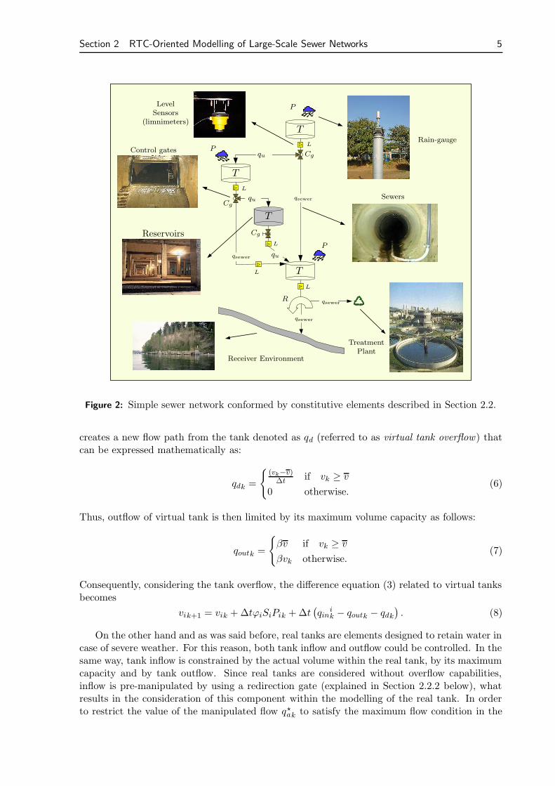
Using the virtual tank modelling principle and the mass balance conservation law, a sewernetwork can be decomposed and described by using the elementary models explained below andshown in Figures 1 and 2, element by element and conforming a simple network, respectively.Other common sewage system elements such as pumping stations can be easily represented byusing the mentioned modelling principles but will be omitted here as they are not taken intoaccount in the case study presented in this paper. Every outlined element presented belowincludes a conceptual scheme which will be not only used for describing its operation but alsofor explaining the mathematical relations and equations derived when the modelling approachesare explained along the next sections.

2.2.1 Virtual and Real Tanks

These elements are used as storage devices. In the case of virtual tanks, the mass balance ofthe stored volume, the inflows and the outflow of the tank and the input rain intensity can bewritten as the difference equation

vik+1 = vik + ∆tϕiSiPik + ∆t(

qinik − qout

ik

)

, (3)


PSfrag replacements

T

qin

v

qd

qout

vk

(a) Virtual tank

PSfrag replacements

qin

qa

qb

qout

v

vkT

(b) Real tank

PSfrag replacements

qin

qa

qb

qout

vvk

T

qin

qa

qb

(c) Redirection gate

PSfrag replacements

qin

qa

qb

qout

vvk

Tqin

qa

qb

qin

qb

qc

(d) Sewer pipe or weir with singleinflow

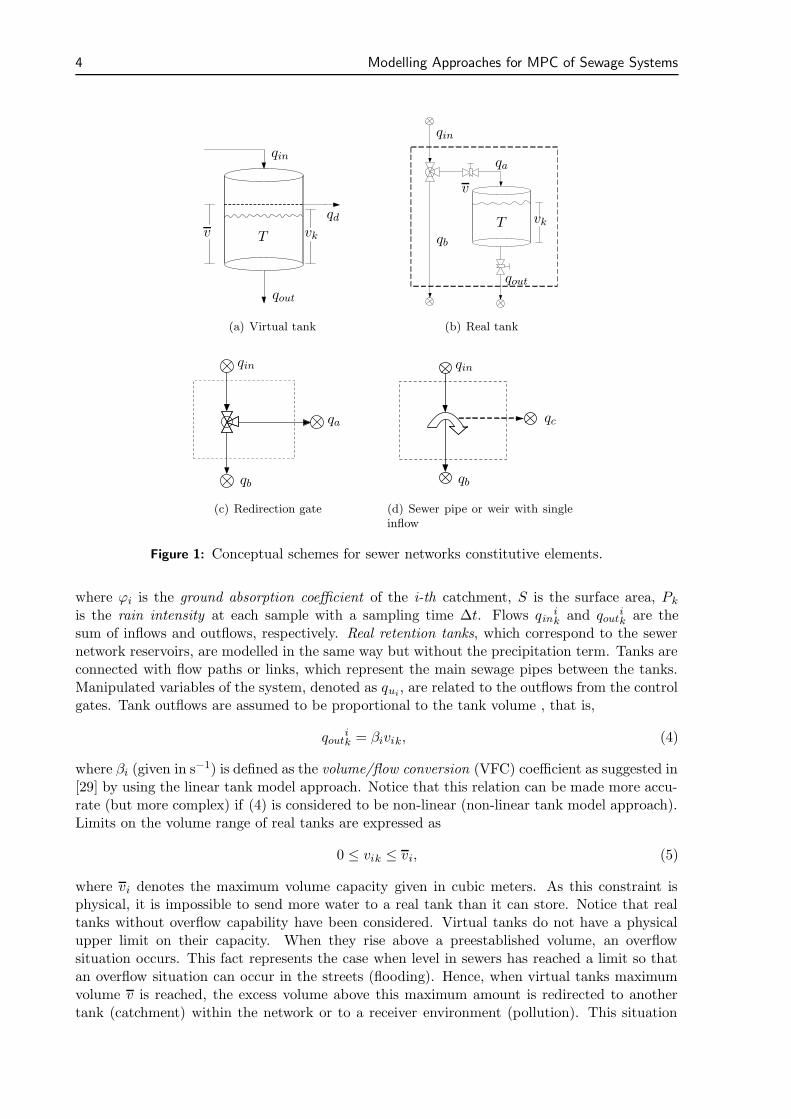
Figure 1: Conceptual schemes for sewer networks constitutive elements.

where ϕi is the ground absorption coefficient of the i-th catchment, S is the surface area, Pk

is the rain intensity at each sample with a sampling time ∆t. Flows qinik and qout

ik are the

sum of inflows and outflows, respectively. Real retention tanks, which correspond to the sewernetwork reservoirs, are modelled in the same way but without the precipitation term. Tanks areconnected with flow paths or links, which represent the main sewage pipes between the tanks.Manipulated variables of the system, denoted as qui

, are related to the outflows from the controlgates. Tank outflows are assumed to be proportional to the tank volume , that is,

qoutik = βivik, (4)

where βi (given in s−1) is defined as the volume/flow conversion (VFC) coefficient as suggested in[29] by using the linear tank model approach. Notice that this relation can be made more accu-rate (but more complex) if (4) is considered to be non-linear (non-linear tank model approach).Limits on the volume range of real tanks are expressed as

0 ≤ vik ≤ vi, (5)

where vi denotes the maximum volume capacity given in cubic meters. As this constraint isphysical, it is impossible to send more water to a real tank than it can store. Notice that realtanks without overflow capability have been considered. Virtual tanks do not have a physicalupper limit on their capacity. When they rise above a preestablished volume, an overflowsituation occurs. This fact represents the case when level in sewers has reached a limit so thatan overflow situation can occur in the streets (flooding). Hence, when virtual tanks maximumvolume v is reached, the excess volume above this maximum amount is redirected to anothertank (catchment) within the network or to a receiver environment (pollution). This situation


PSfrag replacements

T

T

T

T

qu

qu

qu

R

qsewer

qsewer

qsewer

qsewer

Cg

Cg

Cg

P

P

P

L

L

L

L

L

Receiver Environment

Sewers

Rain-gauge

Reservoirs

Control gates

LevelSensors

(limnimeters)

TreatmentPlant

Figure 2: Simple sewer network conformed by constitutive elements described in Section 2.2.

creates a new flow path from the tank denoted as qd (referred to as virtual tank overflow) thatcan be expressed mathematically as:

qdk =

{

(vk−v)∆t

if vk ≥ v

0 otherwise.(6)

Thus, outflow of virtual tank is then limited by its maximum volume capacity as follows:

qoutk =

{

βv if vk ≥ v

βvk otherwise.(7)

Consequently, considering the tank overflow, the difference equation (3) related to virtual tanksbecomes

vik+1 = vik + ∆tϕiSiPik + ∆t(

qinik − qoutk − qdk

)

. (8)

On the other hand and as was said before, real tanks are elements designed to retain water incase of severe weather. For this reason, both tank inflow and outflow could be controlled. In thesame way, tank inflow is constrained by the actual volume within the real tank, by its maximumcapacity and by tank outflow. Since real tanks are considered without overflow capabilities,inflow is pre-manipulated by using a redirection gate (explained in Section 2.2.2 below), whatresults in the consideration of this component within the modelling of the real tank. In orderto restrict the value of the manipulated flow q?

ak to satisfy the maximum flow condition in the


input gate, flow through input link qa should be expressed as

qak =

{

q?ak if q?

ak ≤ qink

qink otherwise.(9)

However, maximum tank capacity also restricts the inflow according to the expression

qak =

{

qak if qbk − qoutk ≤v−vk

∆tv−vk

∆totherwise.

(10)

Finally, tank outflow is given by

qoutk =

{

q?outk if q?

outk ≤ βvk

βvk otherwise,(11)

taking into account that q?out is also restricted by the maximum capacity of the outflow link,

denoted by qoutk. Thus, latter expressions lead to the following difference equation for real tanksin sewer networks:

vk+1 = vk + ∆t(qak − qoutk). (12)

Notice that the flow through qb corresponds to the mass balance

qbk = qink − qak. (13)

Figures 1(a) and 1(b) show conceptual schemes of the both virtual and real tanks considered inthis paper.

2.2.2 Manipulated Gates

Within a sewer network, gates are elemets used as control devices since they can change the flowdownstream. Depending on the action made, gates can be classified as retention gates, used tochange the direction of the sewage flow, and redirection gates, used to retain the sewage flow ina certain point (sewer or reservoir) of the network. In the case of real tanks, a retention gateis present to control the outflow. Virtual tank outflows can not be closed but can be divertedusing redirection gates. Indeed, redirection gates divert a flow from a nominal path which theflow follows if the gate is closed. This nominal flow is denoted as Qi in the equation below,which expresses the mass conservation relation of the element:

qoutik = Qik +

∑

j

qjuik

, (14)

where j is an index over all manipulated flows coming from the gate. Figure 1(c) shows aconceptual scheme of redirection gates considered in this paper. Assuming that the flow throughsewer qa is imposed (for instance computed by means of a control law), the expressions thatdescribe a redirection gate can be written as:

qak =

{

qa if q?a > qa

q?a otherwise,

(15)

where q?a corresponds to the imposed/computed value for the flow qak. Flow qbk is directly given

by the mass balance expressionqbk = qink − qak. (16)


2.2.3 Weirs and Main Sewer Pipes

These components complement the set of elements of sewer networks considered in this paper.Since the descriptions of their dynamics are relatively close, all of them are presented togetherin this section. Nodes are points of the network where the sewage can be either propagated ormerged. Hence, these elements can be classified as splitting nodes and merging nodes. The firsttype can be treated considering a constant partition of the sewage flow in predefined portionsaccording to the topological design characteristics. Indeed, splitting nodes exhibit a switchingbehaviour. In the case of a set of n inflows qi, with i = 1, 2, . . . , n, the expression for the nodeoutflow qout is written as

qout =n∑

i=0

qi. (17)

Weirs can be seen as splitting nodes having a maximum capacity in the nominal outflow pathrelated to the flow capacity of the output pipe. In the same way, main sewer pipes can be seenas weirs with a single inflow. They are used as connection devices between network constitutiveelements. Therefore, considering the similarity between all the aforementioned elements and thenotation in Figure 1(d), the set of expressions valid to represent the behaviour either a weir ora sewer pipe are the following:

qbk =

{

qb if qin > qb

qink otherwise,(18a)

qck =

{

qink − qb if qin > qb

0 otherwise,(18b)

where qb is the maximum flow through qb and qin is the inflow. Notice that the outflow fromvirtual tanks is assumed to be unlimited in order to guarantee a feasible solution of an associatedoptimization problem within the design procedure of a optimization-based control strategy. Thesame idea applies to the outflow qbk related to retention gates. But most often, sewer pipes havelimited flow capacity. The description of this element given here takes into account this limitedcapacity. When the limit of flow capacity is exceeded, resulting overflow is possibly redirectedto another element within the network or is considered as loss to the environment.

2.3 Hybrid Modelling Approach using MLD Forms

In order to obtain a control-oriented model that takes into account the switching elementsand discontinuous phenomena inherent of sewage systems (as presented in previous section),the hybrid systems modelling methodology based on MLD forms proposed by [16] is brieflydescribed.

According to [16], an entire sewer network model is constructed by connecting the systeminflows (rain) and outflows (sewer treatment plants and/or outflows to the environment) withthe inflows and outflows of the elements as well as connecting the elements themselves. Theset of manipulated variables of the whole sewage system, denoted as qu, is conformed by themanipulated variables of the constitutive elements of the sewer network. The logical conditionspresented to describe the dynamics of the sewage system elements can be translated into linearinteger inequalities as described in [2]. The whole sewer network expressed in MLD form can bewritten as

vk+1 = Avk + B1quk + B2δk + B3zk + B4dk, (19a)

yk = Cvk + D1quk + D2δk + D3zk + D4dk, (19b)

E2δk + E3zk ≤ E1quk + E4vk + E5 + E6dk, (19c)


where v ∈ Rnc+ corresponds to the vector of tank volumes (states), qu ∈ R

mic+ is the vector of

manipulated sewer flows (inputs), d ∈ Rmd+ is the vector of rain measurements (disturbances),

logic vector δ ∈ {0, 1}r` collects the Boolean overflow conditions and vector z ∈ Rrc+ is associated

with variables that appear depending on system states and inputs. Variables δ and z are auxiliaryvariables associated with the MLD form. Equation (19c) collects the set of element constraintsas well as translations from logic propositions. Notice that this model is a more general MLDthan was presented in [2] due to the addition of the measured disturbances.

Next, the set of logical conditions needed to describe the dynamics of the sewage systemelements presented in Section 2.2 are outlined for each considered constitutive element.

2.3.1 Virtual Tanks

The overflow existence condition in this element is considered by defining the logical variable

[δk = 1]←→ [vk ≥ v], (20)

what implies that flows qdk and qoutk are defined through this logical variable as:

z1k = qdk

= δk

[

(vk − v)

∆t

]

, (21a)

z2k = qoutk

= δkβv + (1− δk)βvk. (21b)

Hence, the corresponding difference equation for the tank in function of the auxiliary variablesis rewritten as:

vk+1 = vk + ∆t[qink − z1k − z2k], (22)

where qink is the tank inflow, z1k is related to the tank overflow and z2k is related to the tankoutput. Notice that qink collects all inflows to the tank, which could be outflows from tankslocated upstream, link flows, overflows from other tanks and/or sewers and rain inflows. Flowqbk is computed as in (13).

2.3.2 Real Tanks

The MLD form for a real tank and manipulated input/output gates according to the descriptionin Section 2.2.1 can be obtained by introducing the set of δ and z variables collected in Table 1.

Table 1: Expressions for δ and z variables for hybrid modelling of the real tank element.

Logical variable δ Auxiliary variable z

[δ1k = 1]←→ [q?a ≤ qink] z1k = qbk = δ1kq

?ak + (1− δ1k)qink

[δ2k = 1]←→[

z1k − z3k ≤v−vk

∆t

]

z2k = qak = δ2kqbk + (1− δ2k)v−vk

∆t

[δ3k = 1]←→ [q?out ≤ βvk] z3k = qoutk = δ3kq

?outk + (1− δ3k)βvk

Then, mass balance difference equation of real tanks can be rewritten as follows:

vk+1 = vk + ∆t[z3k − z2k]. (23)

Again, flow qbk is computed as in (13).


2.3.3 Redirection Gates

The MLD form is obtained taking into account that qa, i.e., the manipulated flow (see Figure1(c)), should satisfy the restriction (15). Hence, definitions

[δk = 1]←→ [qak ≥ qink] (24)

and

zk = δ1kqak + (1− δ1k)qink (25)

are stated in order to generate the MLD form of this element. Thus, the flow through sewer qb

is directly defined by the mass conservation relation

qbk = qink − zk. (26)

2.3.4 Main Sewer Pipes (or Single Inflow Weirs)

The MLD form for either of these elements is obtained from the overflow condition

[δk = 1]←→ [qin ≥ qb], (27)

and the auxiliary continuous variables that define the flows qbk and qck are, respectively:

z1k = qbk

= δk qb + (1− δk) qink, (28a)

z2k = qck

= δk (qink − qb). (28b)

2.4 PWL Modelling Approach

An alternative approach to the hybrid modelling consists in using continuous and monotonicfunctions to represent expressions that contains logical conditions, as for instance, (6) or (18),which describe the weirs behaviour and overflow capability of reservoirs, respectively. Indeed,these phenomena involve the switching and discontinuous behaviour of the sewage system.

The properties of a function being monotonic and continuous are very useful when optimization-based control strategies are designed since a quasi-convex optimization problem can be stated,what might lead in a global optimal solution [4]. The continuous and monotonic functions forthe modelling approach proposed here are defined as follows:

• Saturation function, defined as

sat(x,M) =

x if 0 ≤ x ≤M,

M if x > M,

0 if x < 0.

(29)

• Dead-zone function, defined as

dzn(x,M) =

{

x−M if x ≥M,

0 if x < M.(30)

Next, sewer network constitutive elements described in Section 2.2 will be expressed usingthis modelling approach. Notice that the whole representation of a given sewer network modelledusing this approach consists in a set of equations instead of a matricial model as the one obtainedwith the hybrid MLD approach presented in previous section.


2.4.1 Virtual Tanks

Using the PWLF approach, the tank outflows can be expressed as

qoutk = β sat (vk, vk) , (31)

qdk =dzn(vk, vk)

∆t, (32)

what allows the difference equation for the tank volume to be written as in (12):

vk+1 = vk + ∆t(qink − qdk − qoutk), (33)

where qink considers all possible inflows including the precipitation term (in flow units).

2.4.2 Real Tanks

The following expressions related to the tank inflow and outflow are stated for this element:

qoutk = sat (q?outk, β vk) , (34)

qak = sat

(

q?ak,min

(

vk − vk

∆t, qink

))

. (35)

Thus, the difference equation for the volume of the tank is again written as in (12):

vk+1 = vk + ∆t(qak − qoutk), (36)

and flow qb obeys to the mass balance qbk = qink − qak.

2.4.3 Redirection Gates

In the case of redirection gates, the PWLF model is defined taking into account that qa shouldsatisfy the restriction (15) what can be rewritten in terms of the PWL functions as

qak = sat(qak, qink). (37)

Flow through qb is given by the mass balance (16).

2.4.4 Main Sewer Pipes (or Single Inflow Weirs)

The PWLF model for either of these elements can be obtained from the overflow condition asfollows:

qbk = sat(qink, qb), (38)

qck = dzn(qink, qb), (39)

where qb corresponds again to the maximum flow capacity of the nominal outflow pipe.

3 MPC-Based RTC on Large-scale Sewer Networks

3.1 MPC as a Tool for Implementing Global RTC

In most sewer networks, the regulated elements (pumps, gates and detention tanks) are typicallycontrolled locally, i.e., they are controlled by a remote station according to the measurementsof sensors connected to that station only. However, a global RTC system requires the use of anoperational model of the network dynamics in order to compute, ahead of time, optimal control

Section 3 MPC-Based RTC on Large-scale Sewer Networks 11

strategies for the network actuators based on the current state of the system (provided bySCADA1 sensors), the current rain intensity measurements and appropriate rainfall predictions.The computation procedure of an optimal global control law should take into account all thephysical and operational constraints of the sewage system, producing set-points which achieveminimum flooding and CSO.

As discussed in the introduction, MPC is a suitable control strategy to implement globalRTC of sewer networks since it has some features to deal with complex systems such as sewernetworks: big delays compensation, use of physical constraints, relatively simple for peoplewithout deep knowledge of control, multivariable systems handling, etc. Hence, according to[27], such controllers are very suitable to be used in the global control of urban drainage systemswithin a hierarchical control structure [21, 14].

MPC, which more than a control technique, is a set of control methodologies that use amathematical model of a considered system to obtain a control signal minimizing a cost functionrelated to selected performance indexes related to the system behaviour. MPC is very flexibleregarding its implementation and can be used over almost all systems since it is set according tothe model of the plant [5]. Notice that MPC, as the global control law, determines the referencesfor local controllers located on different elements of the sewer network. A management level isused to provide to MPC the operational objectives, what is reflected in the controller design asthe performance indexes to be minimized. In the case of urban drainage systems, these indexesare usually related to flooding, pollution, control energy, etc.

This section briefly describes the MPC strategy from the generic point of view and thendescribes the particularities for its use with sewage systems.

3.2 MPC Strategy Description

MPC is a wide field of control methods that share a set of basic elements in common as

• a cost function, that represents a performance index of the system studied,

• a prediction model, which should capture the representative process dynamics and allowsto predict the future behaviour of the system, and

• a control signal computation procedure using a receding horizon strategy generally bysolving an optimization problem whose objective is the cost function and the restrictionsare the prediction model plus the operational constraints.

However, different tuning parameters rise to a different set of implementation algorithms [12].

3.3 General MPC Formulation

MPC strategy used in this paper follows the formulation introduced in [12]. Thus, let

xk+1 = g(xk, uk) (40)

be the mapping of states xk ∈ X ⊆ Rn and control signals uk ∈ U ⊆ R

m for a given system,where g : Rn ×R

m → Rn is a function that describes the system. In the case of this paper, g

can be either a MLD or PWLF model obtaided by using the elementary models presented inSection 2.

Let

uk(xk) ,(

u0|k, u1|k, . . . , uHp−1|k

)

∈ UHp (41)

1Supervisory Control And Data Adquisition (SCADA)


be an input control sequence over a fixed time horizon Hp. Then, an admissible input sequencewith respect to the state xk ∈ X is defined by

UHp(xk) ,{

uk ∈ UHp |xk ∈ X

Hp}

, (42)

where

xk(xk,uk) ,(

x1|k, x2|k, . . . , xHp|k

)

∈ XHp (43)

corresponds to the state sequence generated by applying the input sequence (41) to the system(40) from initial state x0|k , xk, where xk is the measurement (or the estimation) of thecurrent state. Hence, the receding horizon approach is based on the solution of the open-loopoptimization problem (OOP) [3]

min{uk∈ UHp}

J (uk, xk,Hp) , (44a)

subject to

H1uk ≤ b1, (44b)

G2xk + H2uk ≤ b2, (44c)

where J(·) : Xf (Hp) 7→ R+ is the cost function with domain in the set of feasible statesXf (Hp) ⊆ X [11], Hp denotes the prediction horizon or output horizon and G2, Hi and bi

are matrices of suitable dimensions. In sequence (43), xk+i|k denotes the prediction of the stateat time k + i done in k , starting from x0|k = xk. When Hp = ∞, the OOP is called infinitehorizon problem, while with Hp 6= ∞, the OOP is called finite horizon problem. Constrainsstated to guarantee system stability in closed loop would be added in (44b)-(44c).

Assuming that the OOP (44) is feasible for x ∈ X, i.e., UHp(x) 6= ∅, there exists an optimalsolution given by the sequence

u∗k ,

(

u∗0|k, u

∗1|k, . . . , u

∗Hp−1|k

)

∈ UHp , (45)

and then the receding horizon philosophy sets [12], [5]

uMPC(xk) , u∗0|k, (46)

and disregards the computed inputs from k = 1 to k = Hp − 1, repeating the whole processat the following time step. Equation (46) is known in the MPC literature as the MPC law.Summarizing, Algorithm 1 briefly describes the basic MPC law computing process.

Algorithm 1 Basic MPC law computation.

1: k = 02: loop3: xk+0|k = xk

4: u∗k(xk)⇐ solve OOP (44)

5: Apply only uk = u∗k+0|k

6: k = k + 17: end loop

Section 3 MPC-Based RTC on Large-scale Sewer Networks 13

3.4 MPC on Sewer Networks

3.4.1 Control Objectives

The sewage system control problem has multiple objectives with varying priority, see [14]. Thetype, number and priority of those objectives can also be different depending on the particularsewage system design. However, in general, the most common objectives are related to themanipulation of the sewage in order to avoid undesired sewage flows outside of the main sewers(flooding). Another type of control objectives are related for instance to the control energy, i.e.,the energy cost of the regulation gates movements. The main considered objectives for the casestudy presented in this paper are listed below in order of decreasing priority:

• Objective 1: minimize flooding in streets (virtual tank overflow).

• Objective 2: minimize flooding in links between virtual tanks.

• Objective 3: maximize sewage treatment.

A secondary purpose of the third objective is to reduce the volume in the tanks to anticipatefuture rainstorms. This objective also indirectly reduces pollution to the environment. This isbecause if the treatment plants are used optimally with the storage capacity of the network,pollution should be strongly minimized. Moreover, this objective can be complemented byconditioning minimum volume in real tanks at the end of the prediction horizon. It could beseen as a fourth objective. It should be noted that in practice the difference between the firsttwo objectives is small.

3.4.2 Problem Constraints

When using the modelling approach based on virtual tanks either in MLD or PWLF form,only flow rates are manipulated in such way that some the inherent nonlinearities (e.g., non-linear relation between gate opening and discharge flow) of the sewer network are simplified asdiscussed in [10]. But, in turn, some physical restrictions need to be included as constraints onsystem variables. For instance, variables q

jui that redirect outflow from a virtual tank should

never be larger than the outflow from the tank. This is expressed with the following inequality

∑

j

qjuik≤ qout

ik = β vik (47)

Additionally, operational constraints associated to the range of gates actuation leads tothe manipulated flows has to fulfill q

juik ≤ q

jui, where q

jui denotes its upper limit. Similarly,

operational limits on the range of real tank volumes should be included (see (5)) to limit theamount of sewage that can be stored.

3.4.3 MPC disturbances

Rain plays the role of measured disturbance in the MPC problem on sewer networks. The type ofdisturbance model to be used depends on the rain prediction procedure available [30]. Existingmethods include from the use of time series [30] to the sophisticated utilization of meteorologicalradars [33]. According to [14], different assumptions can be done for the rain prediction whenan optimal control law is used in the RTC of sewer networks. Results show that the assumptionof constant rain over a short prediction horizon gives results that can be compared with theassumption of known rain over the considered horizon, confirming similar results are reportedin [10] and [19].


4 Case Study Description

4.1 The Barcelona Sewer Network

The city of Barcelona has a CSS of approximately 1697 km length in the municipal area plus335 Km in the metropolitan area, but only 514.43 km are considered as the main sewer network.Its storage capacity is of 3038622 m3, which implies a dimension three times greater than othercities comparable to Barcelona. It is worth to notice that Barcelona has a population which isaround 1.59 million inhabitants on a surface of 98km2, approximately. This fact results in a veryhigh density of population. Additionally, the yearly rainfall is not very high (600mm/year), butit includes heavy storms (up to 90mm/h) typical of the Mediterranean climate that can cause alot of flooding problems and CSO to the receiving environments.

Clavegueram de Barcelona, S.A. (CLABSA) is the company in charge of the sewage systemmanagement in Barcelona. There is a remote control system in operation since 1994 which in-cludes, sensors, regulators, remote stations, communications and a Control Center in CLABSA.Nowadays, as regulators, the urban drainage system contains 21 pumping stations, 36 gates,10 valves and 8 detention tanks which are regulated in order to prevent flooding and CSO.The remote control system is equipped with 56 remote stations including 23 rain-gauges and136 water-level sensors which provide real-time information about rainfall and water levels intothe sewage system. All this information is centralized at the CLABSA Control Center througha SCADA system. The regulated elements (pumps, gates and detention tanks) are currentlycontrolled locally, i.e., they are handled from the remote control center according to the mea-surements of sensors connected only to local stations.

4.2 Barcelona Test Catchment

From the whole sewer network of Barcelona, which was described beforehand, this paper con-siders a portion that represents the main phenomena and the most common characteristicsappeared in the entire network. This representative portion is selected to be the case study ofthis paper because a calibrated and validated model of the network obtained using the virtualmodelling methodology (see Section 2) is available as well as rain gauge data for an interval ofseveral years. The considered Barcelona Test Catchment (BTC) has a surface of 22,6 km2 andincludes typical elements of the larger network.

The BTC has one retention gate associated with one real tank, three redirection gates andone retention gate, 11 sub-catchments defining equal number virtual tanks, several level gauges(limnimeters) and a two WWTPs. Also, there are five rain-gauges used to measure the rainentering in each sub-catchment. Notice that some sub-catchments (virtual tanks) share thesame rain sensor. These sensors count the amount of tipping events in five minutes (samplingtime) and such values is multiplied by 1.2 mm/h in order to obtain the rain intensity P in m/sat each sampling time, after the appropriate units conversion. The difference between the raininflows for virtual tanks that share sensor lies in the surface area Si and the ground absorbtioncoefficient ϕi of the i-th sub-catchment (see (3)), what yields in different amount of the raininflows.

Using the virtual tanks representation principle, resulting BTC model has 12 state vari-ables corresponding to the volumes in the 12 tanks (one real, 11 virtual), four control inputscorresponding to the manipulated links and five measured disturbances corresponding to themeasurements of rain precipitation at the sub-catchments. Two WWTPs are used to treat thesewage before it is released to the environment. It is supposed that all states (virtual tankvolumes) are estimated by using the limnimeters shown with capital letter L in Figure 3. Thefree flows to the environment as pollution (q10M, q7M, q8M and q11M to the Mediterranean seaand q12s to other catchment) and the flows to the WWTPs (q7L and q11B) are also shown in

Section 4 Case Study Description 15

PSfrag replacements

T1

T2

T3

T4

T5

T5

T6

T7

T8

T9

T10

T11

T12

qu1

qu2

qu3

qu4

R1

R2

R3

R4

R5

q14

q24

q96

q910

qc210

q945

q946

q10M

q57

q68

q7M

q128

q12s

q811

q8M

q11B

q11M

q7L

C1

C4

C2

C3

P13

P14

P16

P16

P16

P19

P20

P20P20

P20

P20

L39

L41

L80

L16

L53

L9

L27

L

L

L3

L11

L47

L56

L7

L8

Mediterranean

Sea

Escola

Industrial

tank

Weir overflowdevice

Real tank

Virtualtank

rainfall

Level gauge

Redirectiongate

Retention gate

gate

(WWTP 1)LlobregatTreatment

Plant

(WWTP 2)Bess

TreatmentPlant

Figure 3: Barcelona test catchment scheme.

the figure as well as rain intensities P13, P14, P16, P19 and P20 according to the case. The fourmanipulated links, denoted as qui

have a maximum flow capacity of 9.14, 25, 7 and 29.3 m3/ s,respectively, and these amounts can not be relaxed, being physical restrictions of the system(hard constraints).


Table 2: Rain episodes used for comparing modelling approaches

Rain Maximum Return Return RateEpisode Rate (years) average (years)

1999-09-14 16.3 4.32002-07-31 8.3 1.02002-10-09 2.8 0.61999-10-17 1.2 0.72000-09-28 1.1 0.4

4.3 Rain Episodes

Rain episodes used for the simulation of the BTC and for the design of MPC strategies arebased on real rain gauge data obtained within the city of Barcelona on the given dates (yyyy-mm-dd) as presented in Table 2. These episodes were selected to represent the meteorologicalbehaviour of Barcelona, i.e., they contain representative meteorologic phenomena in the city.Table 2 also shows the maximum return rate2 among all five rain gauges for each episode. Inthe third column of the table, the return rate for the whole Barcelona network is shown. Thenumber is lower because it includes in total 20 rain gauges. Notice that one of the rain stormshad a return rate of 4.3 years in the case of the whole network while for one of the rain gaugesthe return rate was 16.3 years.

5 Simulation and Results

5.1 Preliminaries

This section is focused on comparing the performance of a MPC-based sewer network RTCusing a set of real rain episodes in Table 2 when the hybrid and PWLF modelling approaches,proposed in Section 2, are applied to the case study in Section 4. Computation time, when everymodelling approach is used, is also compared. Results of such comparison would be a key issueto decide which of the two modelling approaches should be used for a RTC implementation inthe real network. The assumptions made for all the implementations will be presented and theirvalidity discussed before the results are given.

The detailed description of BTC case study including operating ranges of the control signalsand state variables as well as the description of all variables and parameters can be found in[16] and [17].

The computation times presented in this paper has been obtained using Matlabr 7.2 im-plementations running on an Intelr CoreTM2, 2.4 GHz machine with 4Gb RAM. Notice thatcomputation time results reported here related with hybrid models are different with respect to[16] due to the machine characteristics and solver versions.

5.2 Simulation and Prediction Models

Results presented in this paper are obtained in simulation by using two different models: oneused as the plant (sewer network), which in the sequel will be called as open-loop model, and theother used by the MPC controller or prediction model. The open-loop model is implemented con-sidering a non-linear representation of the sewer network based on mass balances where ranges

2The return rate or return period is defined as the average interval of time within which a hydrological eventof given magnitude is expected to be equaled or exceeded exactly once. In general, this amount is given in years.

Section 5 Simulation and Results 17

and bounds for every variable (control signals, volumes, rain disturbances) are strictly consid-ered and all passible logical or discontinuous dynamics are included (as the case of weirs andoverflows). On the other hand, prediction model is obtained by using the modelling approachespresented in Section 2.

To obtain a model of the BTC using the hybrid modelling approach, the elementary modelsand transformations presented in Section 2 should be used. However, in order to avoid thetedious procedure of deriving the MLD form of the BTC by hand, the higher level languageand associated compiler Hysdel (see [31]) are used here. The resulting model in MLD formhas 22 logical variables and 44 auxiliary variables. Once the hybrid model based on MLD formhas been obtained, a hybrid MPC controller has been designed and the set of considered rainscenarios were simulated using the Hybrid Toolbox for Matlabr (see [1]) and Ilog Cplex 11.2.This latter solver allows to solve efficiently the MIP problems associated to the hybrid MPCcontroller. Using the hybrid model, to determine the control actions using hybrid MPC impliesthat for each time instant, considering a prediction horizon Hp = 6, 222×6 = 5.4 × 1039 LPproblems (for a linear norm in the cost function) or QP problems (for a quadratic norm in thecost function) should be solved in the worst case.

On the other hand, the model of BTC using the PWLF-based modelling approach wasobtained by joining the different compositional elements described in Section and following thenetwork diagram of Figure 3, resulting in a non-linear representation as a set of expressions forthe whole network. The implementation of an MPC using the PWLF modelling approach leadsto a non-linear optimization problem. The selection of the algorithm to solve such problemwas done after the evaluation of several solvers available on Tomlabr (e.g., conSolve, nlpSolve,among others). The Structured Trust Region algorithm (see [7]) was finally chosen because itprovides an acceptable trade-off between system performance and computation time.

5.3 MPC Controller Set-up

Different parameters of the MPC controller should be defined and tuned according to the controlobjectives and their prioritization. Following the discussion in Section 3.4.1 regarding the controlobjectives of a sewer network, the following system outputs have been included in both the hybridand PWLF modelling approaches:

y1k =∑

i

qstrv k +∑

j

qstrq k, (48a)

y2k =∑

l

qseak, (48b)

y3k = qtrp1k, (48c)

y4k = qtrp2k, (48d)

where y1k represents the sum of the i overflows to street from virtual tanks at time k, denotedby qstrv k, plus the sum of the j overflows to street from links (main pipes) at time k, denoted byqstrq k

. Output y2k represents the sum of the l overflows which go to sea (as receiver environment)at time k, denoted as qseav k, and finally y3k and y3k represent the flows towards the WWTPs attime k, denoted by qtrp1k and qtrp2k. Note that for the case study of this paper, qtrp1k = q7Lk

and qtrp1k = q11Bk.

Using the outputs (48), the cost function for the BTC can be written as follows

J(uk, xk) =

Hp−1∑

i=0

∥

∥yk+i|k − yr

∥

∥

2

Q, (49)


where yk+i|k is the output vector (defined by (48)) at the instant k + i with respect to timeinstant k, Hp denotes the prediction horizon and yr is a known vector containing the systemreferences and defined for this case as

yr = [0 0 1T q7L 1

T q11B]T , (50)

where 1 is a vector of ones with suitable dimensions and q7L and q11B correspond to the maximumflow capacity through sewers q7L and q11B, respectively.

In order to tune the MPC controller, the weighted approach technique has been used. Hence,in (49), Q corresponds to the weight matrix containing the weights wi, each one related to acontrol objective. Notice that the desired prioritization of the control objectives is given by thevalues wi that, for this case, determine a Q matrix of the following form:

Q = diag{wstr I wsea I wtrp1 I wtrp2 I}, (51)

where I corresponds to a identity matrix of suitable dimensions. Here, wstr = 1, wsea = 10−1,wtrp1 = 10−3, and wtrp2 = 10−3.

The prediction horizon Hp has been set to 6, which is equivalent to 30 minutes with asampling time ∆t = 300s. This selection was based on the reaction time of the system todisturbances. Another reason for this selection is that the constant rain prediction assumed inthis paper becomes less reliable for larger horizons. The length of the simulation scenarios is 100samples, what allows to see the influence of the peak of the rain (disturbance) from the selectedrain episode over the dynamics of the network and also over the dynamic of the closed loop.

5.4 Control performance and computation time comparisons

In this section, the comparison between results obtained using the MPC controllers based onthe hybrid and PWLF modelling approaches is presented and discussed. Moreover, results forthe performance indexes when the open-loop scheme is simulated are also outlined. This lattercase consists in the sewage system without control so the manipulated links are used as passiveelements, i.e., the amount of flows qu1, qu2 and qu4 only depend on the inflow to the correspondinggate and they are not manipulated while qu3 is the outflow of the real tank given by gravity(tank discharge). Results related to the control performance are summarized in Tables 3, 4, and5 for five of the more representative rain episodes in Barcelona between 1998 and 2002 (yyyy-mm-dd in tables). Table 3 shows the comparison of the volumes of sewage that go to street(flooding) during a simulation scenario while Table 4 shows the same comparison but regardingthe volumes to receiver environments (pollution). Finally, Table 5 shows the comparison ofvolumes regarding the treated sewage at the WWTPs.

Table 3: Performance results. Index: Flooding [×103 m3].

Rain Episodes Open Loop Hybrid Model PWLF Model

1999-09-14 108 92.9 88.22002-10-09 116.1 97 113.32002-07-31 160.3 139.7 132.81999-10-17 0 0 02000-09-28 1 1 1

Notice from Tables 3, 4, and 5 that the performance of the system is better when a MPCcontrol law is considered no matter the modelling approach utilized with respect to the perfor-mance in open-loop. This justifies the use of closed-loop control. Moreover, notice also that

Section 5 Simulation and Results 19

Table 4: Performance results. Index: Pollution (×103 m3].


1999-09-14 225.8 223.5 226.1 (1.16%)

2002-10-09 409.8 398.7 407.7 (2.25%)

2002-07-31 378 374.6 380 (1.44%)

1999-10-17 65 58.1 59.9 (3.09%)

2000-09-28 104.5 98 102 (4.08%)

Table 5: Performance results. Index: Treated sewage at WWTPs (×103 m3].


1999-09-14 278.3 280.7 276.7 (1.43%)

2002-10-09 533.8 545 534.2 (1.98%)

2002-07-31 324.3 327.8 321.9 (1.80%)

1999-10-17 288.4 295.3 293.5 (0.61%)

2000-09-28 285.3 291.9 287.5 (1.51%)

the use of the hybrid modelling approach implies in average an better system performance (al-ways respecting the prioritization of the control objectives) with respect to the performanceimprovement obtained by using the PWLF modelling approach. Notice also that the perfor-mance improvement is basically related to the improvement of the main control objective andthen, following in a hierarchical order, to the second objective and so on.

These results, in general, were expected since the MPC controller based on the hybrid mod-elling approach achieves its optimum by solving a set of convex linear programs using a branchand bound scheme. However, the MPC based on PWLF modelling approach leads to a non-linear network model representation what results in a non-convex optimization. Therefore, theglobal optimum can not be assured leading possibly to a sequence of suboptimal controls whenthe computation of the receding horizon control law is done. This explains why the performanceobtained using the PWLF model is in general worse than the one obtained using the hybridmodel. However, it is very difficult to ensure that the optima reached for a complex problemthat involves multi-objectives optimization and trial and error tuning procedures is the suitablefor the particular case study. Suboptimality levels of the results obtained using the PWLFmodel were never greater that 4.1 % for the cases of the second and third objective (as shownin Tables 4, and 5 in parenthesis at the last column for some rain episodes). For the case ofthe first control objective (related to flooding), results were not so homogeneous since for somescenarios one of the modelling approaches leads in better system performance while for otherscenarios occurred just the opposite.

On the other hand, the main difference of using the hybrid or the PWLF modelling ap-proaches is in the computation time required to compute the control actions at each iteration.As mentioned in Section 5.2, the model in MLD form contains an important number of Booleanand auxiliary variables. The complexity of the MIP associated to the MPC law becomes big-ger by increasing the number of Bolean variables since the underlying optimization problemis combinatorial and NP-hard [20]. Thus, the worst-case computation time is exponential inthe amount of integer variables. In large-scale systems such as a sewer network, the amountof elements with logical/discontinuous dynamics can augment according to the topology of theparticular case study. Therefore, computation times increase towards a point where the use ofthis modelling for obtaining a MPC-based RTC law becomes almost impossible. On the other

20 REFERENCES

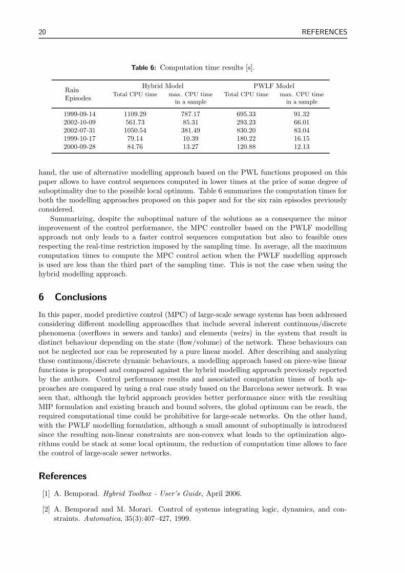
Table 6: Computation time results [s].

RainEpisodes

Hybrid Model PWLF ModelTotal CPU time max. CPU time

in a sampleTotal CPU time max. CPU time

in a sample

1999-09-14 1109.29 787.17 695.33 91.322002-10-09 561.73 85.31 293.23 66.012002-07-31 1050.54 381.49 830.20 83.041999-10-17 79.14 10.39 180.22 16.152000-09-28 84.76 13.27 120.88 12.13

hand, the use of alternative modelling approach based on the PWL functions proposed on thispaper allows to have control sequences computed in lower times at the price of some degree ofsuboptimality due to the possible local optimum. Table 6 summarizes the computation times forboth the modelling approaches proposed on this paper and for the six rain episodes previouslyconsidered.

Summarizing, despite the suboptimal nature of the solutions as a consequence the minorimprovement of the control performance, the MPC controller based on the PWLF modellingapproach not only leads to a faster control sequences computation but also to feasible onesrespecting the real-time restriction imposed by the sampling time. In average, all the maximumcomputation times to compute the MPC control action when the PWLF modelling approachis used are less than the third part of the sampling time. This is not the case when using thehybrid modelling approach.

6 Conclusions

In this paper, model predictive control (MPC) of large-scale sewage systems has been addressedconsidering different modelling approacdhes that include several inherent continuous/discretephenomena (overflows in sewers and tanks) and elements (weirs) in the system that result indistinct behaviour depending on the state (flow/volume) of the network. These behaviours cannot be neglected nor can be represented by a pure linear model. After describing and analyzingthese continuous/discrete dynamic behaviours, a modelling approach based on piece-wise linearfunctions is proposed and compared against the hybrid modelling approach previously reportedby the authors. Control performance results and associated computation times of both ap-proaches are compared by using a real case study based on the Barcelona sewer network. It wasseen that, although the hybrid approach provides better performance since with the resultingMIP formulation and existing branch and bound solvers, the global optimum can be reach, therequired computational time could be prohibitive for large-scale networks. On the other hand,with the PWLF modelling formulation, although a small amount of suboptimally is introducedsince the resulting non-linear constraints are non-convex what leads to the optimization algo-rithms could be stack at some local optimum, the reduction of computation time allows to facethe control of large-scale sewer networks.

References

[1] A. Bemporad. Hybrid Toolbox - User’s Guide, April 2006.

[2] A. Bemporad and M. Morari. Control of systems integrating logic, dynamics, and con-straints. Automatica, 35(3):407–427, 1999.

REFERENCES 21

[3] A. Bemporad and M. Morari. Robust model predictive control: A survey. In A. Garulli,A. Tesi, and A. Vicino, editors, Robustness in Identification and Control, number 245, pages207–226. Springer-Verlag, 1999.

[4] S. Boyd and L. Vandenberghe. Convex Optimization. Cambridge University Press, 2004.

[5] E.F. Camacho and C. Bordons. Model Predictive Control. Springer-Verlag, London, secondedition, 2004.

[6] G. Cembrano, J. Quevedo, M. Salamero, V. Puig, J. Figueras, and J. Mart. Optimal controlof urban drainage systems: a case study. Control Engineering Practice, 12(1):1–9, 2004.

[7] A. R. Conn, N. Gould, A. Sartenaer, and Ph. L. Toint. Convergence properties of mini-mization algorithms for convex constraints using a structured trust region. SIAM Journalon Optimization, 6(4):1059–1086, 1995.

[8] S. Duchesne, A. Mailhot, E. Dequidt, and J. Villeneuve. Mathematical modeling of sewersunder surcharge for real time control of combined sewer overflows. Urban Water, 3:241–252,2001.

[9] Y. Ermolin. Mathematical modelling for optimized control of Moscow’s sewer network.Applied Mathematical Modelling, 23:543–556, 1999.

[10] M. Gelormino and N. Ricker. Model predictive control of a combined sewer system. Inter-national Journal of Control, 59:793–816, 1994.

[11] M. Lazar, W.P.M.H. Heemels, S. Weiland, and A. Bemporad. Stability of hybrid modelpredictive control. IEEE Transactions of Automatic Control, 51(11):1813 – 1818, 2006.

[12] J.M. Maciejowski. Predictive Control with Constraints. Prentice Hall, Great Britain, 2002.

[13] M. Marinaki and M. Papageorgiou. Nonlinear optimal flow control for sewer networks.In Proceedings of the IEEE American Control Conference, volume 2, pages 1289–1293,Philadelphia, Pennsylvania, USA, 1998.

[14] M. Marinaki and M. Papageorgiou. Optimal Real-time Control of Sewer Networks. Springer,2005.

[15] L.W. Mays. Urban Stormwater Management Tools. McGrawHill, 2004.

[16] C. Ocampo-Martinez. Model Predictive Control of Complex Systems including Fault Tol-erance Capabilities: Application to Sewer Networks. PhD thesis, Technical University ofCatalonia, April 2007.

[17] C. Ocampo-Martinez, A. Bemporad, A. Ingimundarson, and V. Puig. On hybrid modelpredictive control of sewer networks. In R. Sanchez-Pena, V. Puig, and J. Quevedo, editors,Identification & Control: The gap between theory and practice. Springer-Verlag, 2007.

[18] C. Ocampo-Martinez, A. Ingimundarson, V. Puig, and J. Quevedo. Objective prioritizationusing lexicographic minimizers for MPC of sewer networks. IEEE Transactions on ControlSystems Technology, 16(1):113–121, 2008.

[19] C. Ocampo-Martinez, V. Puig, J. Quevedo, and A. Ingimundarson. Fault tolerant modelpredictive control applied on the Barcelona sewer network. In Proceedings of IEEE Con-ference on Decision and Control (CDC) and European Control Conference (ECC), Seville(Spain), 2005.

22 REFERENCES

[20] C. Papadimitriou. Computational Complexity. Addison-Wesley, 1994.

[21] M. Papageorgiou. Optimal multireservoir network control by the discrete maximum prin-ciple. Water Resour. Res., 21(12):1824 – 1830, 1985.

[22] M. Pleau, H. Colas, P. Lavalle, G. Pelletier, and R. Bonin. Global optimal real-time controlof the Quebec urban drainage system. Environmental Modelling & Software, 20:401–413,2005.

[23] M. Pleau, F. Methot, A. Lebrun, and A. Colas. Minimizing combined sewer overflow inreal-time control applications. Water Quality Research Journal of Canada, 31(4):775 – 786,1996.

[24] M. Schechter. Polyhedral functions and multiparametric linear programming. Journal ofOptimization Theory and Applications, 53:269–280, 1987.

[25] W. Schilling, B. Anderson, U. Nyberg, H. Aspegren, W. Rauch, and P. Harremes. Real-timecontrol of wasterwater systems. Journal of Hydraulic Resourses, 34(6):785–797, 1996.

[26] M. Schtze, D. Butler, and B. Beck. Modelling, Simulation and Control of Urban WastewaterSystems. Springer, 2002.

[27] M. Schutze, A. Campisanob, H. Colas, W.Schillingd, and P. Vanrolleghem. Real timecontrol of urban wastewater systems: Where do we stand today? Journal of Hydrology,299:335–348, 2004.

[28] M. Schutze, T. To, U. Jaumar, and D. Butler. Multi-objective control of urban wastewatersystems. In Proceedings of 15th IFAC World Congress, Barcelona, Spain, 2002.

[29] V.P Singh. Hydrologic systems: Rainfall-runoff modeling, volume I. Prentice-Hall, N.J.,1988.

[30] K.T. Smith and G.L. Austin. Nowcasting precipitation - A proposal for a way forward.Journal of Hydrology, 239:34–45, 2000.

[31] F. Torrisi and A. Bemporad. Hysdel - A tool for generating computational hybrid modelsfor analysis and synthesis problems. IEEE Trans. Contr. Syst. Technol., 12(2):235–249,2004.

[32] M. Weyand. Real-time control in combined sewer systems in Germany: Some case studies.Urban Water, 4:347 – 354, 2002.

[33] J.M. Yuan, K.A. Tilford, H.Y. Jiang, and I.D. Cluckie. Real-time urban drainage systemmodelling using weather radar rainfall data. Phys. Chem. Earth (B), 24:915–919, 1999.

IRI reports

This report is in the series of IRI technical reports.All IRI technical reports are available for download at the IRI websitehttp://www.iri.upc.edu.

modelling approaches for predictive control of large-scale

Documents