modelling concurrent computations: from contextual petri...
TRANSCRIPT

Universita degli Studi di Pisa
Dipartimento di Informatica
Dottorato di Ricerca in Informatica
Ph.D. Thesis: TD-1/00
Modelling Concurrent Computations:
from Contextual Petri Nets
to Graph Grammars
Paolo Baldan
March 2000
Addr: Corso Italia 40, 56125 Pisa, ItalyTel: +39-050-887268 — Fax: +39-050-887226 — E-mail: [email protected]
http://www.di.unipi.it/~ baldan

Thesis Supervisors:Dott. Andrea Corradini and Prof. Ugo Montanari

Abstract
Graph grammars (or graph transformation systems), originally introduced as a gen-eralization of string grammars, can be seen as a powerful formalism for the speci-fication of concurrent and distributed systems, which properly extends Petri nets.The idea is that the state of a distributed system can be naturally represented (ata suitable level of abstraction) as a graph and local state transformations can beexpressed as production applications.
With the aim of consolidating the foundations of the concurrency theory forgraph transformation systems, the thesis extends to this more general setting somefundamental approaches to the semantics coming from Petri net theory. More specif-ically, focusing on the so-called double pushout (dpo) algebraic approach to graphrewriting, the thesis provides graph transformation systems with truly concurrentsemantics based on (concatenable) processes and on a Winskel’s style unfoldingconstruction, as well as with more abstract semantics based on event structures anddomains.
The first part of the thesis studies two generalizations of Petri nets, alreadyknown in the literature, which reveal a close relationship with graph transformationsystems, namely contextual nets (also called nets with read, activator or test arcs)and inhibitor nets (or nets with inhibitor arcs). Extending Winskel’s seminal workon safe nets, the truly concurrent semantics of contextual nets is given via a chainof coreflections leading from the category of contextual nets to the category of fini-tary coherent prime algebraic domains. A basic role is played by asymmetric eventstructures, which generalize prime event structures by allowing a non-symmetricconflict relation. The work is then generalized to inhibitor nets, where, due to thenon-monotonicity of the enabling, the causal structure of computations is far morecomplex, and a new, very general, notion of event structure, called inhibitor eventstructure, is needed to faithfully describe them.
The second part of the thesis, relying on the conceptual basis drawn in thefirst part, focuses on graph grammars. Inhibitor event structures turn out to beexpressive enough to model graph grammar computations, and the theory developedfor contextual and inhibitor nets, comprising the unfolding and the (concatenable)process semantics, can be lifted to graph grammars. The developed semantics isshown to to be consistent also with the classical theory of concurrency for dpograph grammars relying on shift-equivalence.


To Alessandra.


Acknowledgments
Not surprisingly, the people I am most indebted to are my advisors, Ugo Montanariand Andrea Corradini, who followed and supported me with high competence duringmy PhD studies. They have been a constant source of ideas and suggestions whichhave played a fundamental role in the development of the material in this thesis.
I surely cannot forget to thank Furio Honsell and Fabio Alessi, the advisors ofmy master thesis in Udine. There, I moved my first steps in the world of research,learning the importance of aesthetic criteria, like elegance and beauty, in the evalu-ation of scientific productions, and I understood that it is possible (and necessary)to enjoy working.
Many thanks are due to my external reviewers, Philippe Darondeau and HartmutEhrig, for their careful reading of a preliminary version of this thesis, and for theiruseful comments and suggestions. I would like to express my gratitude also to GiorgioGhelli and Andrea Maggiolo Schettini, who followed the annual advancement of mythesis work during the last three years.
I took full advantage from my participation to the getgrats project, whichoffered me the opportunity of meeting and discussing with several people. In partic-ular, I would like to remember Martin Große-Rhode, Reiko Heckel, Manuel Koch,Marta Simeoni and Francesco Parisi Presicce. I would like to acknowledge also NadiaBusi and Michele Pinna who provided me some useful hints to improve the materialin Chapter 3.
I want to thank also my colleagues and friends at the Department of ComputerScience in Pisa, who contributed to create a nice and stimulating (not only from thescientific viewpoint) working environment. When I moved to Pisa to start my PhDcourse, from the very beginning I found many kind people who received me in thebest way. In particular I would like to mention Simone Martini, Andrea Masini andLaura Semini who helped me with their friendship and with many useful advices,and Giorgio Ghelli and Maria Simi who kindly hosted me in their office. I would liketo thank Giorgio also for the pleasure I had working with him.
Then, many many people with whom I had courses, meals and discussions haveinfluenced positively the quality of my staying at the department. Roberto Bruni,Gianluigi Ferrari, Fabio Gadducci and Merce Llabres Segura (a guest who has im-mediately become part of the “family”) besides being very good friends (or perhapsjust for this), read a preliminary version of the thesis helping me to greatly improve

the presentation. A special thank goes to Roberto for the never-ending discussions hehas always accepted to engage on disparate subjects. The long working days (oftencontinuing through nights) have been less hard for the presence of my roommates,from the former ones, Vladimiro Sassone, Marco Pistore and Paola Quaglia to therecent ones, Stefano Bistarelli, Diego Sona and Emilio Tuosto. I also want to thankChiara Bodei and Roberta Gori, with whom I shared the pain of the thesis deadline,the “polemic” Andrea Bracciali, the “comrade” Simone Contiero, Paolo Volpe andFrancesca Scozzari.
Vorrei ringraziare i miei genitori per essermi sempre stati vicini, e ricordare mianonna Cea che e stata per me una seconda madre. Un grazie anche a Leo e Nico, eun benvenuto ad Edoardo.
Infine, un ringraziamento davvero speciale va ad Alessandra, mia moglie e com-pagna di vita. Anche nella preparazione di questa tesi il suo aiuto e stato preziosoe insostituibile . . . vorrei dire altro, ma cadrei presto in luoghi comuni, cosı comespesso accade a chi, non essendo un poeta, si avventuri a parlare di cose per cui leparole non bastano.

Contents
1 Introduction 11.1 Petri nets . . . . . . . . . . . . . . . . . . . . . . . . . . . . . . . . . 31.2 Graph Grammars . . . . . . . . . . . . . . . . . . . . . . . . . . . . . 91.3 Truly concurrent semantics of Petri nets . . . . . . . . . . . . . . . . 13
1.3.1 Semantics of Petri nets . . . . . . . . . . . . . . . . . . . . . . 131.3.2 A view on applications . . . . . . . . . . . . . . . . . . . . . . 161.3.3 The role of category theory . . . . . . . . . . . . . . . . . . . 17
1.4 From Petri nets to graph grammars: an overview of the thesis . . . . 181.4.1 The general approach . . . . . . . . . . . . . . . . . . . . . . . 221.4.2 Summary of the results . . . . . . . . . . . . . . . . . . . . . . 23
1.5 Structure of the thesis . . . . . . . . . . . . . . . . . . . . . . . . . . 24
I Contextual and inhibitor nets 27
2 Background 292.1 Basic notation . . . . . . . . . . . . . . . . . . . . . . . . . . . . . . . 292.2 Contextual and inhibitor nets . . . . . . . . . . . . . . . . . . . . . . 32
2.2.1 Contextual nets . . . . . . . . . . . . . . . . . . . . . . . . . . 322.2.2 Inhibitor nets . . . . . . . . . . . . . . . . . . . . . . . . . . . 332.2.3 Alternative approaches . . . . . . . . . . . . . . . . . . . . . . 34
2.3 Process semantics of generalized Petri nets . . . . . . . . . . . . . . . 352.3.1 Contextual nets . . . . . . . . . . . . . . . . . . . . . . . . . . 362.3.2 Inhibitor nets . . . . . . . . . . . . . . . . . . . . . . . . . . . 37
2.4 Event structures and domains . . . . . . . . . . . . . . . . . . . . . . 372.4.1 Prime event structures . . . . . . . . . . . . . . . . . . . . . . 382.4.2 Prime algebraic domains . . . . . . . . . . . . . . . . . . . . . 392.4.3 Generalized event structure models . . . . . . . . . . . . . . . 42
3 Semantics of Contextual Nets 453.1 Asymmetric conflicts and asymmetric event structures . . . . . . . . 46
3.1.1 Asymmetric event structures . . . . . . . . . . . . . . . . . . . 483.1.2 Morphisms of asymmetric event structures . . . . . . . . . . . 51

ii Contents
3.1.3 Relating asymmetric and prime event structures . . . . . . . . 523.2 From asymmetric event structures to domains . . . . . . . . . . . . . 53
3.2.1 The domain of configurations of an aes . . . . . . . . . . . . . 543.2.2 A coreflection between AES and Dom . . . . . . . . . . . . . 59
3.3 The category of contextual nets . . . . . . . . . . . . . . . . . . . . . 633.4 Occurrence contextual nets . . . . . . . . . . . . . . . . . . . . . . . . 65
3.4.1 Dependency relations on transitions . . . . . . . . . . . . . . . 663.4.2 Concurrency and reachability . . . . . . . . . . . . . . . . . . 683.4.3 Morphisms on occurrence c-nets . . . . . . . . . . . . . . . . . 71
3.5 Unfolding: from semi-weighted to occurrence contextual nets . . . . . 743.6 Occurrence contextual nets and asymmetric event structures . . . . . 793.7 Processes of c-nets and their relation with the unfolding . . . . . . . . 85
3.7.1 Contextual nets processes . . . . . . . . . . . . . . . . . . . . 883.7.2 Concatenable processes . . . . . . . . . . . . . . . . . . . . . . 893.7.3 Relating processes and unfolding . . . . . . . . . . . . . . . . 91
4 Semantics of Inhibitor Nets 974.1 Inhibitor event structures . . . . . . . . . . . . . . . . . . . . . . . . . 98
4.1.1 Inhibitor event structures and their dependency relations . . . 994.1.2 Morphisms of inhibitor event structures . . . . . . . . . . . . . 1024.1.3 Relating asymmetric and inhibitor event structures . . . . . . 107
4.2 From inhibitor event structures to domains . . . . . . . . . . . . . . . 1084.2.1 The domain of configurations of an ies . . . . . . . . . . . . . 1084.2.2 A coreflection between IES and Dom . . . . . . . . . . . . . 1144.2.3 Removing non-executable events . . . . . . . . . . . . . . . . . 120
4.3 The category of inhibitor nets . . . . . . . . . . . . . . . . . . . . . . 1234.4 Occurrence i-nets and unfolding construction . . . . . . . . . . . . . . 1254.5 Inhibitor event structure semantics for i-nets . . . . . . . . . . . . . . 129
4.5.1 From occurrence i-nets to ies’s . . . . . . . . . . . . . . . . . 1304.5.2 From ies’s to i-nets: a negative result . . . . . . . . . . . . . . 132
4.6 Processes of i-nets and their relation with the unfolding . . . . . . . . 135
Summary and Final Remarks 141
II Semantics of DPO Graph Grammars 145
5 Typed Graph Grammars in the DPO Approach 1475.1 Basic definitions . . . . . . . . . . . . . . . . . . . . . . . . . . . . . . 147
5.1.1 Relation with Petri nets . . . . . . . . . . . . . . . . . . . . . 1555.2 Derivation trace semantics . . . . . . . . . . . . . . . . . . . . . . . . 157
5.2.1 Abstraction equivalence and abstract derivations . . . . . . . . 1585.2.2 Shift equivalence and derivation traces . . . . . . . . . . . . . 161

Contents iii
5.3 A category of typed graph grammars . . . . . . . . . . . . . . . . . . 1665.3.1 From multirelations to spans . . . . . . . . . . . . . . . . . . . 1665.3.2 Graph grammar morphisms . . . . . . . . . . . . . . . . . . . 1715.3.3 Preservation of the behaviour . . . . . . . . . . . . . . . . . . 173
6 Unfolding and Event Structure Semantics 1776.1 Nondeterministic occurrence grammars . . . . . . . . . . . . . . . . . 1796.2 Nondeterministic graph processes . . . . . . . . . . . . . . . . . . . . 1866.3 Unfolding construction . . . . . . . . . . . . . . . . . . . . . . . . . . 1896.4 The unfolding as a universal construction . . . . . . . . . . . . . . . . 192
6.4.1 Unfolding of semi-weighted graph grammars . . . . . . . . . . 1926.4.2 Unfolding of general grammars . . . . . . . . . . . . . . . . . 198
6.5 From occurrence grammars to event structures . . . . . . . . . . . . . 2006.5.1 An IES semantics for graph grammars . . . . . . . . . . . . . 2016.5.2 A simpler characterization of the domain semantics . . . . . . 204
6.6 Unfolding of SPO graph grammars . . . . . . . . . . . . . . . . . . . 206
7 Concatenable Graph Processes 2097.1 Deterministic graph processes . . . . . . . . . . . . . . . . . . . . . . 2107.2 Concatenable graph processes . . . . . . . . . . . . . . . . . . . . . . 2137.3 Relating derivation traces and processes . . . . . . . . . . . . . . . . 216
7.3.1 Characterization of the ctc-equivalence . . . . . . . . . . . . . 2167.3.2 From processes to traces and backwards . . . . . . . . . . . . 220
7.4 Relating unfolding and deterministic processes . . . . . . . . . . . . . 225
8 Relation with Other Event Structure Semantics 2298.1 Event structure from concatenable traces . . . . . . . . . . . . . . . . 2298.2 Event structure semantics from deterministic derivations . . . . . . . 232
Summary and Final Remarks 235
9 Conclusions 237
A Basic Category Theory 241A.1 Functors . . . . . . . . . . . . . . . . . . . . . . . . . . . . . . . . . . 243A.2 Natural transformations . . . . . . . . . . . . . . . . . . . . . . . . . 244A.3 Universal properties, limits and colimits . . . . . . . . . . . . . . . . 245A.4 Adjunctions . . . . . . . . . . . . . . . . . . . . . . . . . . . . . . . . 248A.5 Comma category constructions . . . . . . . . . . . . . . . . . . . . . . 250
Bibliography 253


List of Figures
1.1 A simple Petri net. . . . . . . . . . . . . . . . . . . . . . . . . . . . . 41.2 Traditional nets do not allow for concurrent read-only operations. . . 51.3 The contextual net process corresponding to a transaction. . . . . . . 71.4 The contextual net processes for two possible schedulings of the transactions T ′ and T ′′.1.5 Representing priorities via inhibitor arcs. . . . . . . . . . . . . . . . . 81.6 A (double-pushout) graph rewriting step. . . . . . . . . . . . . . . . . 101.7 A graph grammar representation of system Ring. . . . . . . . . . . . 111.8 A Petri net representation of system Ring. . . . . . . . . . . . . . . . 121.9 A semi-weighted P/T net, which is not safe. . . . . . . . . . . . . . . 161.10 Asymmetric conflict in contextual nets. . . . . . . . . . . . . . . . . . 201.11 Two basic nets with inhibitor arc. . . . . . . . . . . . . . . . . . . . . 21
2.1 Different notions of enabling in the literature. . . . . . . . . . . . . . 352.2 A flow event structure F such that there are no bundle event structures with the same configurations.
3.1 A simple contextual net and a prime event structure representing its behaviour. 473.2 A contextual net for which pes’s with possible events are not adequate. 483.3 A pre-aes with two conflictual events e and e′, not related by asymmetric conflict. 503.4 An occurrence c-net with a cycle of asymmetric conflict. . . . . . . . 673.5 A c-net and (part of ) its unfolding. . . . . . . . . . . . . . . . . . . . 763.6 Three simple aes’s and the corresponding occurrence c-nets produced by the functor Na.3.7 The (a) aes (b) domain and (c) pes for the c-net N of Figure 3.5 . . 863.8 aes semantics is finer than pes semantics. . . . . . . . . . . . . . . . 87
4.1 Two basic inhibitor nets. . . . . . . . . . . . . . . . . . . . . . . . . . 994.2 The pes corresponding to the ies where (e′, e, e0, . . . , en). . . 1204.3 Functors relating semi-weighted (occurrence) c-nets and i-nets. . . . . 1264.4 Not all events of an occurrence i-net are executable. . . . . . . . . . . 127
5.1 Pushout diagram. . . . . . . . . . . . . . . . . . . . . . . . . . . . . . 149
5.2 (a) The parallel production 〈(q1, in1), . . . , (qk, in
k)〉 : (Ll← K
r→ R) and (b) its compact represen
5.3 (Parallel) direct derivation as double-pushout construction. . . . . . . 1525.4 Productions, start graph and graph of types of the grammar C -S modelling client-server5.5 A derivation of grammar C -S starting from graph G0. . . . . . . . . 155

vi List of Figures
5.6 A (parallel) derivation, with explicit drawing of the s-th production of the i-th direct derivation.5.7 Firing of a transition and corresponding dpo derivation. . . . . . . . 1565.8 Abstraction equivalence of decorated derivations (the arrows in productions spans are not lab5.9 Sequential independent derivations. . . . . . . . . . . . . . . . . . . . 1625.10 Local confluence of independent direct derivations. . . . . . . . . . . . 1635.11 A derivation ρ′ in grammar C -S , shift-equivalent to derivation ρ of Figure 5.6.1655.12 Equivalence and composition of spans. . . . . . . . . . . . . . . . . . 1685.13 The spans f1 (left diagram) and f2 (right diagram) in Set. . . . . . . 1685.14 Computing the image of a multiset. . . . . . . . . . . . . . . . . . . . 1705.15 Graph grammars morphisms preserve derivations. . . . . . . . . . . . 176
6.1 Two safe grammars and their net-like representation. . . . . . . . . . 1816.2 The inhibitor nets corresponding to the grammars G1 and G2 in Figure 6.1.1826.3 Graph processes. . . . . . . . . . . . . . . . . . . . . . . . . . . . . . 1876.4 Graph process isomorphism. . . . . . . . . . . . . . . . . . . . . . . . 1896.5 The construction mapping safe grammars into i-nets is not functorial. 1946.6 The grammars G1 and G2, and the pullback-retyping diagram for their start graphs.1996.7 Encoding asymmetric conflict and dangling condition in prime event structures.206
7.1 A graph process of the grammar C -S . . . . . . . . . . . . . . . . . . 2127.2 From abstract concatenable processes to concatenable derivation traces and backward.221
8.1 Event structure of the grammar C -S . . . . . . . . . . . . . . . . . . 232
A.1 Associativity and identity diagrams for arrow composition. . . . . . . 243A.2 Naturality square of the transformation η : F
·−→ G : A→ B for the arrow f ∈ A.245
A.3 The diagrams for (i) products and (ii) coproducts. . . . . . . . . . . 246A.4 Commutative cone. . . . . . . . . . . . . . . . . . . . . . . . . . . . . 247A.5 An arrow h from the cone p′ to p. . . . . . . . . . . . . . . . . . . . . 247A.6 Diagrams for (i) pullback and (ii) pushout. . . . . . . . . . . . . . . . 248A.7 The left adjoint F . . . . . . . . . . . . . . . . . . . . . . . . . . . . . 249A.8 The definition of the right adjoint to F . . . . . . . . . . . . . . . . . . 249A.9 The right adjoint G. . . . . . . . . . . . . . . . . . . . . . . . . . . . 250A.10 Arrows in the comma category 〈F ↓ G〉. . . . . . . . . . . . . . . . . 251A.11 Category of objects under/over a given object. . . . . . . . . . . . . . 251

Chapter 1
Introduction
Over the last thirty years there has been a steadily growing interest in concurrent anddistributed systems. An unbroken thread leads from the more classical ideas relatedto the sharing of many computing resources among various users (multiuser systems,databases, etc.) and the use of many distinct computing resources to obtain a greatercomputational power (multiprocessor computing), to the current widespread diffu-sion of Internet and network applications. Day by day real systems become morecomplex and sophisticated, but at the same time more difficult to test and verify,and thus possibly more unreliable. Because of this, new formal models adequate toease the specification, development and verification of concurrent systems are calledfor.
Generally speaking, a formal model must give a representation of a system whichis abstract enough to disregard unnecessary details, and, at the same time, is suf-ficiently rich to allow one to represent properties and aspects of the system whichmay be relevant for the design and verification activities. Besides representing thestate and the architectural aspects of a system, a model typically comes equippedwith an operational semantics which formally explains how the system behaves. Ontop of the concrete operational description, depending on which observations onewants to take into account, more abstract semantics can be introduced. At this levelone can define techniques for checking the equivalence of systems with respect tothe selected observations, for verifying if a systems satisfies a given property, forsynthesizing in an efficient way a system satisfying a given property, etc.
For sequential systems it is often sufficient to consider an input/output semanticsand thus the appropriate semantic domain is usually a suitable class of functionsfrom the input to the output domains. When concurrent or distributed features areinvolved, instead, typically more information about the actual computation of thesystem has to be recorded in the semantic domain. For instance, one may wantto know which steps of computation are independent (concurrent), which steps arecausally related and which steps represent the (nondeterministic) choice points. Thisinformation is necessary, for example, if one wants to have a compositional semantics,allowing to reduce the complexity of the analysis of concurrent systems built from

2 Chapter 1. Introduction
smaller parts, or if one wants to allocate a computation on a distributed architecture.Roughly speaking, nondeterminism can be represented either by collecting all thepossible different computations in a set, or by merging the different computations ina unique branching structure where the choice points are explicitly represented. Onthe other hand, concurrent aspects can be represented by using a truly concurrentapproach, where the causal dependencies among events are described directly in thesemantics using a partially ordered structure. There is some agreement in consid-ering this choice more appropriate for the analysis of concurrent and distributedsystems than the interleaving approach, where concurrency is confused with nonde-terminism, in the sense that the concurrent execution of events is represented as thenondeterministic choice among the possible interleavings of such events.
Petri nets are one of the the most widely used models of concurrency, which hasattracted, since its introduction, the interest of both theoreticians and practitioners.Along the years Petri nets have been equipped with satisfactory semantics, makingjustice of their intrinsically concurrent nature and which have served as basis forthe development of a variety of modelling and verification techniques. However, thesimplicity of Petri nets, which is one of the reasons of their success, represents also alimit in their expressiveness. If one is interested in giving a more structured descrip-tion of the state, or if the kind of dependencies between steps of computation cannotbe reduced simply to causality and conflict, Petri nets are likely to be inadequate.
This thesis is part of a project aimed at proposing graph transformation systemsas an alternative model of concurrency, extending Petri nets. The basic intuitionunderlying the use of graph transformation systems for formal specifications is torepresent the states of a system as graphs (possibly attributed with data-values) andstate transformations by means of rule-based graph transformations. Since a rule hasonly a local effect on the state, it is natural to allow for the parallel application ofrules acting on different parts of the state, a fact that makes graph transformationsystems suited for the representation of concurrency.
Needless to say, the idea of representing system states by means of graphs ispervasive in computer science. Whenever one is interested in giving an explicit rep-resentation of the interconnections, or more generally of the relationships among thevarious components of a system, a natural solutions is to use (possibly hierarchicaland attributed) graphs. The possibility of giving a suggestive pictorial representa-tion of graphical states makes them adequate for the description of the meaning of asystem specification, even to a non-technical audience. A popular example of graph-based specification language is given by the Unified Modeling Language (UML). InUML the conceptual models of system states, the collection of admissible states, and,on an higher level, the distribution of systems are represented by means of diagrams,which are of course graphs, sometimes attributed with textual information. Recallalso the more classical Entity/Relationship (ER) approach, where graphs are usedto specify the conceptual organization of the data, or Statecharts, a specificationlanguage suited for reactive systems, where states are organized in a hierarchicaltree-like structure. Furthermore, graphs provides a privileged representation of sys-

1.1. Petri nets 3
tems consisting of a set of processes communicating through ports. When one isinterested in modelling the dynamic aspects of systems whose states have a graphi-cal nature, graph transformation systems are clearly one of the most natural choices.
With the aim of consolidating the foundations of the concurrency theory of graphtransformation systems, this thesis extends to this more general setting some fun-damental approaches to the semantics of Petri nets. More specifically, inspired bythe close relationships existing between nets and graph transformation systems, weprovide graph transformation systems with truly concurrent semantics based on de-terministic processes and on a Winskel-like unfolding construction, as well as withmore abstract semantics based on event structures and domains.
As an intermediate step, we study two generalizations of Petri nets proposed inthe literature, which reveal a close relationship with graph transformation systems,namely contextual nets (also called nets with read, activator or test arcs) and netswith inhibitor arcs. Due to their relatively wide diffusion, we believe that the workon these extended kinds of nets may be understood as an additional outcome ofthe thesis, independently from its usefulness in carrying out our program on graphtransformation systems.
The rest of this introductory chapter is aimed at presenting the general frame-work in which this thesis has been developed, the main motivations and conceptsfrom Petri net theory, and an overview of the results. First, in Sections 1.1 and 1.2,we give a description of the basic models, namely ordinary Petri nets, contextualand inhibitor nets and finally graph transformation systems, organized in an idealchain where each model generalizes its predecessor. Then Section 1.3 outlines theapproach to the truly concurrent semantics of ordinary Petri nets which we proposeas a paradigm. Section 1.4 gives an overview of the thesis, by explaining how thesemantical framework of ordinary nets has been lifted along the chain of models,first to contextual and inhibitor nets and then to graph grammars. We give a flavourof the main problems which we encountered and we outline the main achievementsof the thesis. Finally, Section 1.5 describes how the thesis is organized and explainsthe origin of the chapters.
1.1 Petri nets
Petri nets, introduced by Carl Adam Petri in the early Sixties [Pet62] (seealso [Rei85]), are one of the most widely accepted models of concurrent and dis-tributed systems, and one of the rare meeting point of theoreticians and practition-ers. The success of Petri nets in the last thirty years can be measured by lookingnot only at the uncountably many applications of nets, but also at the developmentof the theoretical aspects, which range from a complete analysis of the various phe-nomena arising in simple models to the definition of more expressive (and complex)classes of nets.

4 Chapter 1. Introduction
•
s0
•
s1
t0s2 s3
t1 t2 t3
Figure 1.1: A simple Petri net.
One of the reasons of the popularity of Petri nets is probably the simplicity ofthe basic model, whose behaviour, at a fundamental level, can be understood simplyin terms of the so-called token game. The state of a net is a set of tokens distributedamong a set of places. A transition is enabled in a state if enough tokens are presentin the places in its pre-set. The firing of the transition removes some tokens andproduces new tokens in its postconditions.
Petri nets admit a very pleasant and simple graphical representation where placesare drawn as circles, transitions as rectangular boxes and arrows are used to rep-resent the flow relation, specifying which resources are consumed and produced byeach transition. To visualize the state of the net, usually called marking, the tokensare depicted as bullets inside the corresponding places. For instance, in the net ofFigure 1.1, the transition t0 consumes two tokens, one from s0 and one from s1, andthus it is enabled in the represented marking. Its firing produces the new markingwhere s0 and s1 are empty and a new token is produced both in s2 and s3.
The above informal description is probably sufficient to suggest the appropriate-ness of nets as models of concurrency. The state of a net has an intrinsic distributednature, and a transition modifies a local part of the state, making natural to allowthe concurrent firing of transitions when they consume mutually disjoint sets of to-kens (e.g., t2 and t3 in the state produced after the firing of t0). A situation of mutualexclusion is naturally represented by two transitions competing for a single token,like t1 and t2 in the figure. The nondeterministic behaviour of a net is intimatelyconnected with such kind of situations.
A limit in the expressiveness of Petri nets is represented by the fact that atransition can only consume and produce tokens, and thus a net cannot express in anatural way activities which involves non-destructive testing operations on resources.In the following we review contextual nets and inhibitor nets, two generalizations ofclassical nets aimed at overcoming this limit.

1.1. Petri nets 5
N0
• •
t0 •s
t1
• •
t0 •s
t1 N1
Figure 1.2: Traditional nets do not allow for concurrent read-only operations.
Contextual nets.
Contextual nets [MR95], also called nets with test arcs in [CH93], activator arcs in[JK95] or read arcs in [Vog96], extend classical nets with the possibility of checkingfor the presence of tokens which are not consumed. Concretely, besides the usualpreconditions and postconditions, a transition of a contextual net has also somecontext conditions, which specify that the presence of some tokens in certain places isnecessary to enable the transition, but such tokens are not affected by the firing of thetransition. In other words, a context can be thought of as a resource which is read butnot consumed by the transition, in the same way as preconditions can be consideredbeing read and consumed and postconditions being simply written. Coherently withthis view, the same token can be used as context by many transitions at the sametime and with multiplicity greater than one by the same transition. For instance, thesituation of two agents, which access a shared resource in a read-only manner can bemodelled directly by the contextual net N0 of Figure 1.2, where the transitions t0 andt1 use the place s as context. According to the informal description of the semanticsof contextual nets, in N0 the transitions t0 and t1 can fire concurrently. Notice thatin the pictorial representation of a contextual net, directed arcs represent, as usual,preconditions and postconditions, while, following [MR95], non-directed (usuallyhorizontal) arcs are used to represent context conditions.
It is worth remarking that the naıve technique of representing the reading of atoken via a consume/produce cycle may cause a loss in concurrency, even if the samemarkings are reachable. For instance, in the net N1 of Figure 1.2, the two transitionst0 and t1 cannot read the shared resource s concurrently, but their accesses must beserialized.
The ability of faithfully representing the “reading of resources” allows contextualnets to model many concrete situations more naturally than classical nets. In re-cent years they have been used to model the concurrent access to shared data (e.g.,reading in a database) [Ris94, DFMR94], to provide concurrent semantics to concur-rent constraint (CC) programs [MR94, BHMR98] where several agents may accessa common store, to model priorities [JK91] and to compare temporal efficiency inasynchronous systems [Vog97a].
As a concrete example we hint how contextual nets allow to face the problem ofserializability of concurrent transactions in the field of databases [Ris94]. Roughly

6 Chapter 1. Introduction
speaking a transaction implements an “activity” on the database by means of asequence of read and write operations, which, starting from a consistent state of thedatabase, produces a new consistent state. When several agents access a databaseit is natural to allow transactions to be executed concurrently. However in this waythe operations of distinct transactions may interleave in an arbitrary way and thismay cause interferences which lead the database to an inconsistent state. To ensurethat the consistency of the state is maintained we must show that the consideredinterleaving, called a scheduling of the transactions, is indeed equivalent to a serialscheduling of the same transactions, where no interleaving is admitted.
A transaction T = t1; . . . ; tn where each ti is a read or write operation canbe represented by means of a contextual net process (formally defined later, inChapter 2). For instance a transaction T ′ = t1; t2; t3, given by
t1 : read(x, y);t2 : write(z);t3 : read(z)
is represented by the process in Figure 1.3. The places labelled by s′, in the left partof the figure, represent the internal state of the agent performing the transaction,which evolves step by step. The places labelled by x, y and z, in the top part ofthe figure, represent the initial values of the variables. A read(x1, . . . , xn) operationis represented by a single transition (e.g., t1 in the figure) which reads the placescorresponding to the current values of x1, . . . , xn. A write(x) operation is insteadrepresented by two transitions (e.g., t21 and t22 in the figure), one consuming theprevious value of x and the other producing a new value for x. The two transitionsare distinct since the write operation does not depend on the previous value of x butonly destroys it. Observe that both read and write operations consume the placecorresponding to the previous internal state of the agent and produce the new state.
Given two transactions T ′ and T ′′ and a scheduling consisting of a possible in-terleaving of their actions, we can construct, in the same way, a correspondingcontextual net process. In [Ris94] it is shown that two such schedulings lead to thesame final state for all the possible interpretation of the transitions if and only ifthe corresponding processes are isomorphic. Hence a scheduling of T ′ and T ′′ is seri-alizable if and only if the corresponding process is isomorphic either to the processfor T ′;T ′′ or to the process for T ′′;T ′.
For example, let T ′ be the transaction defined above and let T ′′ be the transactionconsisting of the only operation
t4 : read(z)
Figure 1.4 reports the processes corresponding to the schedulings (a) t1; t4; t2; t3 andand (b) t1; t2; t4; t3, of T ′ and T ′′. The two processes are not isomorphic, witnessingthat the two schedulings are not equivalent. Indeed observe that in the first schedul-ing t4 read the initial value of the variable z, while in the second scheduling t4 readthe value written in z by t2.

1.1. Petri nets 7
s′ x y z
t1
s′
t21 t22
s′ z
t3
s′
Figure 1.3: The contextual net process corresponding to a transaction.
s′ x y z s′′
t1 t4
s′ s′′
t21 t22
s′ z
t3
s′
s′ x y z s′′
t1 t4
s′ s′′
t21 t22
s′ z
t3
s′
(a) (b)
Figure 1.4: The contextual net processes for two possible schedulings of the trans-actions T ′ and T ′′.

8 Chapter 1. Introduction
t0 t1
Figure 1.5: Representing priorities via inhibitor arcs.
Instead, it is not difficult to realize that the serial schedulings T ′;T ′′ and T ′′;T ′
have associated exactly the processes in Figure 1.4 (a) and (b), respectively. There-fore both the considered schedulings t1; t4; t2; t3 and t1; t2; t4; t3 of T ′ and T ′′ areserializable.
Inhibitor nets
Inhibitor nets (or nets with inhibitor arcs) [AF73] further generalize contextual netswith the possibility of checking not only for the presence, but also for the absence oftokens in a place. For each transition an inhibitor set is defined and the transitionis enabled only if no token is present in the places of its inhibitor set. When a places is in the inhibitor set of a transition t we say that s inhibits (the firing of) t.
While, at a first glance, this could seem a minor extension, it definitely increasesthe expressive power of the model. In fact, many other extensions of ordinary netscan be simulated in a direct way by using nets with inhibitor arcs (see, e.g., [Pet81]).For instance, this is the case for prioritized nets [Hac76, DGV93], where each tran-sition is assigned a priority and whenever two transitions are enabled at a givenmarking, then the transition with the highest priority fires. To have an informalidea of how the encoding may proceed, two transitions t0 and t1 of a prioritizednet, with t0 having the highest priority, may be represented by simply forgettingthe priorities and adding an inhibitor arc, as depicted in Figure 1.5. Observe thatthe fact that a place s inhibits a transition t is graphically represented by drawinga dotted line from s to t, ending with an empty circle.
Indeed the crucial observation is that traditional nets can easily simulate all theoperation of RAM machines, with the exception of the zero-testing. Enriching netswith inhibitor arcs is the simplest extension which allows to overcome this limit, thusgiving the model the computational power of Turing machines [Age74, Kel72, Kos73].
It is worth stressing that while from the point of view of expressiveness Turingcompleteness is surely a desirable property, when analysis is concerned it may be-come a problem since many properties which were known to be decidable for Petrinets become undecidable. The thesis [Bus98] shows that this problem can be par-tially overcome by singling out restricted, but still interesting, subclasses of inhibitor

1.2. Graph Grammars 9
nets for which algorithms and techniques of classical nets may be extended.
1.2 Graph Grammars
The theory of graph grammars (or of graph transformation systems) studies a varietyof formalisms which extend the theory of formal languages in order to deal withstructures more general than strings, like graphs and maps. A graph grammar allowsone to describe finitely a (possibly infinite) collection of graphs, i.e., those graphswhich can be obtained from a start graph through repeated applications of graphproductions. A graph production is a rule of the kind p : L ; R, that specifies that,under certain conditions, once an occurrence (a match) of the left-hand side L in agraph G has been detected, it can be replaced by the right-hand side R. The form ofgraph productions, the notion of match and in general the mechanisms stating howa production can be applied to a graph and what the resulting graph is, depend onthe specific graph rewriting formalism.
Graph grammars have been deeply studied following the classical lines of thetheory of formal languages, namely focusing on the properties of the generatedgraph languages and on their decidability; briefly, on the results of the generationprocess. However, quite early, graph grammars have been recognized as a powerfultool for the specification of concurrent and distributed systems. The basic idea is thatthe state of many distributed systems can be naturally represented (at a suitablelevel of abstraction) as a graph, and (local) transformations of the state can beexpressed as production applications. Thus a stream of research, mainly dealing withthe algebraic approaches, has grown, concentrating on the rewriting process itself,seen as a representation of systems computations, studying properties of derivationsequences, their transformations and equivalences.
Double-pushout algebraic approach
Here we follow the so-called double-pushout (dpo) algebraic approach (dpo ap-proach, for short) [Ehr87], where the basic notions of production and direct deriva-tion are defined in terms of constructions and diagrams in a suitable category. Con-sequently, the resulting theory is very general and flexible, easily adaptable to avery wide range of structures, simply by changing the underlying category. In thisthesis we will concentrate on directed (typed) graphs, but it is easy to realize thatthe results immediately extends also to hypergraphs. The generalization to moregeneral structures and to abstract categories (e.g., to high level replacement sys-tems [EHKPP91]) is instead less trivial and left as a matter of further investigation.
In the dpo approach a graph production consists of a left-hand side graph L, aright-hand side graph R and a (common) interface graph K embedded both in Rand in L, as depicted in the top part of Figure 1.6. Informally, to apply such a rule toa graph G we must find a match, namely an occurrence of its left-hand side L in G.

10 Chapter 1. Introduction
RL
D HG
K
Figure 1.6: A (double-pushout) graph rewriting step.
The rewriting mechanism first removes the part of the left-hand side L which is notin the interface K producing the graph D, and then adds the part of the right-handside R which is not in the interface K, thus obtaining the graph H . Formally, this isobtained by requiring the two squares in Figure 1.6 to be pushouts in the categoryof graphs, hence the name of the approach. The interface graph K is “preserved”:it is necessary to perform the rewriting step, but it is not affected by the step itself,and as such it corresponds to the context of a transition in contextual nets. Noticethat the interface K plays a fundamental role in specifying how the right-handside has to be glued with the graph D. Working without contexts, which for graphgrammars would mean working with productions having an empty interface graphK, the expressive power would drastically decrease: only disconnected subgraphscould be added.
A basic observation belonging to the folklore (see, e.g., [Cor96]) regards the closerelationship existing between graph grammars and Petri nets. Basically a Petri netcan be viewed as a graph transformation system that acts on a restricted kind ofgraphs, namely discrete, labelled graphs (that can be considered as sets of tokenslabelled by places), the productions being the transitions of the net. In this view,general graph transformation systems are a proper extension of ordinary Petri netsin two dimensions:
1. they allow for the specification of context-dependent rewritings, where part ofthe state is required, but not affected by the rewriting step;
2. they allow for a more structured description of the state, that is an arbitrary,possibly non-discrete, graph.
The relevance of the first capability in the representation of concurrent accessesto shared resources has been already stressed when we have presented contextualnets.

1.2. Graph Grammars 11
P P
PP
E
P
E
E
E
P
E
E
R
P
PR
E
P
P
P
P
RE EMov:
P
P
P
P
P
E P
P
P
E
E
Ins:
P
P
P
P
P
EP
P
P E
E
Rem:
Figure 1.7: A graph grammar representation of system Ring.
As for the second capability, even if multisets may be sufficient in many situa-tions, it is easy to believe that graphs are more appropriate when one is interestedin giving an explicit representation of the interconnections among the various com-ponents of the systems, e.g. if one wants to describe the topology of a distributedsystem and the way it evolves.
Furthermore, in a graph transformation system each rewriting step is requiredto preserve the consistency of the graphical structure of the state, namely each stepmust produce a well-defined graph. In the dpo approach this is expressed by the so-called application condition for productions, which, technically, ensures the existenceof the left-pushout of Figure 1.6 for the given match and thus the applicability ofthe rule. The restrictions to the behaviour which are imposed by such requirementhave often a very natural interpretation in the modelled system.
Let us present an example, which even if very simple, may help the reader toget convinced of the gain in expressiveness determined by the use of graphs in placeof multisets. Consider a system Ring consisting of a set of processes using a singlecommon resource which is accessed in mutual exclusion. The processes are connectedto form a ring and the right to access the resource passes from one process to itssuccessor in the ring.
This situation can be modelled by the graph grammar consisting of the startgraph depicted in the left part of Figure 1.7 and the production Mov. The state ofthe system is naturally represented as a graph where processes are nodes labelledby P and the connections are established by means of edges, labelled by E. Thefact that a process has the right to access the resource is represented by adding aloop R to the corresponding node. The behaviour of the system is represented viaproduction Mov, which moves the loop from the node currently holding the resourceits successor in the ring, preserving their connection.

12 Chapter 1. Introduction
P
P P
P
P
P
Figure 1.8: A Petri net representation of system Ring.
One can observe that the same system can be represented also by the Petrinet of Figure 1.8, where processors are modelled as places and the right to accessthe resource is given by the token moving around the ring. This representation issurely reasonable and simple, but conceptually it seems more natural to representthe topology of the system as part of the state and to model the moving of theresource from a processor the its successor via a single rule (ideally applied by somesupervisor of the system).
At a more concrete level one can notice that the net representation is not veryflexible. In fact, consider a slightly different system, where processors are not alwayspart of the ring. The topology of the system can change dynamically, since a pro-cessor can (ask to) be inserted and removed from the ring, with the constraint thatthe processor holding the resource cannot be removed form the ring. While the netof Figure 1.8 cannot be easily extended to deal with the new situation, the graphgrammar of Figure 1.7 can be adapted by just including the two new rules Add andRem for adding and removing a processor from the ring, respectively.
It is worth noting that, since the consistency of the graphical structure of thestate must be preserved, the rule Rem cannot be applied to the processor holdingthe resource because after its removal the loop R would remain dangling. Thereforethe satisfaction of the constraint imposing that the processor holding the resourcecannot be removed is entailed by the basic properties of the rewriting mechanism.
The above observation leads us to another crucial remark. As shown by theexample, to ensure that after each rewriting step the new state is a well definedgraph, before applying a production q which removes a node n we must be sure thatany edge with source or target in n is removed by q as well, otherwise it would remaindangling in the new state. This requirement, a part of the application condition calleddangling condition in the dpo approach, can be interpreted by thinking that theedges with source or target in the node n, not removed by q, inhibits the application

1.3. Truly concurrent semantics of Petri nets 13
of q. This establishes a deep connection between inhibitor nets and graph grammarswhich will be exploited throughout the thesis. Among other things this suggests theappropriateness of graph grammars to model phenomena which can be expressed byusing inhibitor nets.
1.3 Truly concurrent semantics of Petri nets
In this section we describe the approaches to the semantics of Petri nets whichrepresent the starting point of the results presented in this thesis. Then we hint atthe possible applications of such semantics and we comment on the role of categorytheory in its development.
1.3.1 Semantics of Petri nets
Along the years Petri nets have been equipped with several semantics, aimed atdescribing appropriately, at the right degree of abstraction, the truly concurrentnature of net computations. The approach that we propose as a paradigm, comprisesthe semantics based on deterministic processes, whose origin dates back to an earlyproposal by Petri himself [Pet77] and the semantics based on the nondeterministicunfolding introduced in a seminal paper by Nielsen, Plotkin and Winskel [NPW81],and shows how the two may be reconciled in a very satisfactory framework.
Deterministic process semantics
The notion of deterministic process naturally arises when trying to give a trulyconcurrent description of net computations, taking explicitly into account the causalrelationships which rule the occurrences of events in single computations.
Apart from Best-Devillers processes [BD87] which do not account for causality,the prototypical example of process for Petri nets is given by the Goltz-Reisig pro-cesses [GR83]. A Goltz-Reisig process of a net N is a (deterministic) occurrence netO, i.e. a (safe) finite net satisfying suitable acyclicity and conflict freeness proper-ties, plus a mapping to the original net ϕ : O → N . The flow relation induces apartial order on the elements of the net O, which can be naturally interpreted ascausality. The mapping essentially labels the places and transitions of O with placesand transitions of N , in such a way that places in O can be thought of as tokens ina computation of N and transitions of O as occurrences of transition firings in suchcomputation.
A limitation of Goltz-Reisig processes resides in the fact that they cannot beendowed with an operation of sequential composition, meaningful with respect tocausality. The naıve attempt of concatenating a process ϕ1 with target u with asecond one ϕ2, with source u, by merging the source and the target immediately fails.In fact, there are in general, many ways of putting in one-to-one correspondence the
14 Chapter 1. Introduction
maximal places of ϕ1 with the minimal places of ϕ2, respecting the labelling, andthey lead to different resulting processes of the net. The problem is that the placesof a process represent tokens produced in a computations, and tokens in the sameplace should not be confused since they may have different (causal) histories.
Concatenable processes are defined in [DMM96] as Goltz-Reisig processes inwhich minimal and maximal places carrying the same label are linearly ordered.Such an ordering allows one to disambiguate token identities and thus an opera-tion of concatenation can be safely defined. This brings us to the definition of acategory CP[N ] of concatenable processes, in which objects are markings (statesof the net), arrows are processes (computations) and arrow composition models thesequential composition of computations. It turns out that such category is a symmet-ric monoidal category, in which the tensor product represents faithfully the parallelcomposition of processes.
Unfolding semantics
A deterministic process specifies only the meaning of a single, deterministic com-putation of a net. Nondeterminism is captured only implicitly by the existence ofseveral different “non confluent” processes having the same source. Instead the ac-curate description of the fine interplay between concurrency and nondeterminism isone of the most interesting features of Petri nets.
An alternative classical approach to the semantics of Petri nets is based on anunfolding construction, which maps each net into a single denotational structure,representing, in an unambiguous way, all the possible events that can occur in allthe possible computations of the net and the relations existing between them. Thisstructure expresses not only the causal ordering between the events, but also givesan explicit representation of the branching (choice) points of the computations.
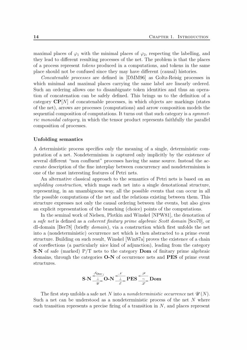
In the seminal work of Nielsen, Plotkin and Winskel [NPW81], the denotation ofa safe net is defined as a coherent finitary prime algebraic Scott domain [Sco70], ordI-domain [Ber78] (briefly domain), via a construction which first unfolds the netinto a (nondeterministic) occurrence net which is then abstracted to a prime eventstructure. Building on such result, Winskel [Win87a] proves the existence of a chainof coreflections (a particularly nice kind of adjunction), leading from the categoryS-N of safe (marked) P/T nets to the category Dom of finitary prime algebraicdomains, through the categories O-N of occurrence nets and PES of prime eventstructures.
S-NU
⊥ O-NE
⊥
IOcc
PESL
∼
N
DomP
The first step unfolds a safe net N into a nondeterministic occurrence net U (N).Such a net can be understood as a nondeterministic process of the net N whereeach transition represents a precise firing of a transition in N , and places represent

1.3. Truly concurrent semantics of Petri nets 15
occurrences of tokens in the places of N . Differently from deterministic processes,the unfolding can be infinite and can contain (forward) conflicts. In this way it cantake advantage of its branching (tree-like) structure to represent all the possiblecomputations of the original net N .
The subsequent step abstracts the occurrence net obtained via the unfoldingconstruction to a prime event structure. Recall that prime event structures (pes)are a simple event based model of (concurrent) computations in which events areconsidered as atomic, indivisible and instantaneous steps, which can appear onlyonce in a computation. An event can occur only after some other events (its causes)have taken place and the execution of an event can inhibit the execution of otherevents. This is formalized via two binary relations: causality, modelled by a partialorder relation ≤ and conflict, modelled by a symmetric and irreflexive relation #,hereditary with respect to causality. The pes semantics is obtained from the unfold-ing simply by forgetting the places, but remembering the basic relations of causalityand conflict between transitions that they induce.
The last step of Winskel’s construction shows that the category of prime eventstructures is equivalent to the category of domains. An element of the domain cor-responding to a pes is a set of events (configuration) which can be understood as apossible computation in the pes. The order (which is simply set inclusion) representsa computational order: if C ⊑ C ′, then C can evolve and become C ′.
In [MMS92, MMS97] it has been shown that essentially the same constructionapplies to the wider category of semi-weighted nets, i.e., P/T nets in which theinitial marking is a set and transitions can generate at most one token in eachpost-condition. It is worth noting that, besides being more general than safe nets,semi-weighted nets present the advantage of being characterized by a “static con-dition”, not involving the behaviour but just the structure of the net. Figure 1.9shows an example of semi-weighted P/T net, which is not safe. The generalizationof Winskel’s construction to the whole category of P/T nets requires some originaltechnical machinery and allows one to obtain a proper adjunction rather than acoreflection [MMS92].
Reconciling deterministic processes and unfolding
Since the unfolding of a net is essentially a nondeterministic process that completelydescribes the behaviour of the net, one would expect that a relation exists betweenthe unfolding and the deterministic process semantics. Indeed, as shown in [MMS96],the domain associated to a net N through the unfolding construction can be equiva-lently characterized as the set of deterministic processes of the net starting from theinitial marking, endowed with a kind of prefix ordering. This result is stated in anelegant categorical way. The comma category 〈m ↓ CP[N ]〉, where m is the initialmarking of the net, is shown to be a preorder (more precisely, this is true for semi-weighted nets, while for general nets a slight variation of the notion of process hasto be considered, called decorated process). Intuitively, the elements of such preorder

16 Chapter 1. Introduction
N2
•s0
•s1
t0 t1s2
2
t2
Figure 1.9: A semi-weighted P/T net, which is not safe.
are computations starting from the initial state, and if ϕ1 and ϕ2 are elements of thepreorder, we have ϕ1 ϕ2 if ϕ1 can be extended to ϕ2 by performing appropriatesteps of computation. Finally, the ideal completion of such preorder, which can beseen as a representation of the (finite and infinite) computations of the net, is shownto be isomorphic to the domain associated to the unfolding.
Deterministic processes
P/T Nets Domains
Unfolding
Although not central in this thesis, we recall that there exists a third approachto Petri net semantics which fits nicely in the above picture, called algebraic seman-tics. Roughly speaking, the algebraic approaches to Petri net semantics, originatedfrom [MM90], characterize net computations as an equational term algebra, freelygenerated starting from the basic elements of the net and having (suitable kindsof) monoidal categories as models. For instance, the category of concatenable pro-cesses can be given a purely algebraic and completely abstract characterization asthe free symmetric strict monoidal category generated by the net N , modulo somesuitable axioms [Sas96]. In particular the distributivity of tensor product and arrowcomposition in monoidal categories is shown to capture the basic facts about netcomputations.
1.3.2 A view on applications
The semantical framework for Petri nets illustrated before, besides being elegantand satisfactory from a theoretical point of view, represents a basis on which thebridge towards applications can be settled. The discussed constructions provide adescription of the behaviour of a net which is, in general, “infinite” and thus appar-ently difficult to deal with. However, on top of them one can build more abstract

1.3. Truly concurrent semantics of Petri nets 17
“approximated” descriptions of the behaviour which turn out to be useful in theverification of several properties of the modelled systems.
The deterministic process and event structure semantics represent the basis forthe definition of history preserving bisimulation [RT88, BDKP91], a bisimulation-like observational equivalence suited to deal with concurrent systems. For instance itis a congruence with respect to some kind of refinement operations and it preservesthe amount of autoconcurrency. History preserving bisimulation is known to bedecidable for n-safe nets, where the number of tokens in each place is bounded by n.Algorithms for checking the bisimilarity of two nets and to get a minimal realizationin a class of bisimilar systems have been proposed in the literature [Vog91, MP98].
Furthermore, although the unfolding is infinite for non trivial nets, as observed byMcMillan in his PhD thesis [McM93], limiting attention to (n-)safe nets it is possibleto construct a finite initial part of the unfolding which contains as much informationas the unfolding itself, the so-called finite complete prefix. The advantage of completeprefixes is that they can be much smaller of the state space of the system, when theyare generated via “clever” algorithms, and, as such, they represent a useful techniqueto attack the well-known state explosion problem of model-checking techniques.Moreover, the information about causality, concurrency and distribution containedin the unfolding may be used to verify properties expressed in local logics, whichallow to reason on the knowledge that each component has of the global state ofthe system. The unfolding technique has been applied to the verification of circuits,telecommunication systems, distributed algorithms, etc.
1.3.3 The role of category theory
Category theory originated as an abstract theory of mathematical structures andof the relationships between structures, aimed at giving a unified view of “similar”results from disparate areas of mathematics.
The categorical language, with its elegance and abstractness, has been exploitedin Computer Science as a tool to give alternative systematic formulations of existingtheories, making clear their real essence and disregarding unnecessary details, andas a guidance for the development and justification of new concepts, properties andresults. The advantages of the use of category theory in Computer Science are wellsummarized in [Gog91]. Here we try to point out some aspects which are particularlyrelevant to our approach.
Considering categories of systems, one is lead to introduce an appropriate notionof morphism between systems, typically formalizing the idea of “simulation”. Thenexpressing the semantics via a functor means to define the semantical transforma-tion consistently with such notion: a morphism between two systems must yield amorphism between their models.
Moreover, the notion of universal construction (e.g., adjunction, reflection, core-flection) provides a formal way to justify the naturality of the semantics, by express-ing its “optimality”. It is often the case that an obvious functor maps models back
18 Chapter 1. Introduction
into the category of systems (e.g., this happens for Petri nets, where occurrence netsare particular nets and thus such a functor is simply the inclusion). Consequentlythe semantics can be defined naturally as the functor in the opposite direction, form-ing an adjunction, which (if it exists) is unique up to natural isomorphism. In otherwords, once one has decided the notion of simulation, there is a unique way to definethe semantics consistently with such notion.
Finally, several composition operations can be naturally expressed at categoricallevel as limit/colimit constructions (products, sums, pushouts, pullbacks, just to cite afew). For instance, a pushout construction can be used to compose two nets, mergingsome part of them, obtaining a kind of generalized nondeterministic composition,while synchronization of nets can be modelled as a product (see [Win87a, MMS97]).
Remarkably, since left/right adjoint functors preserve colimits/limits, a seman-tics defined via an adjunction turns out to be compositional with respect to suchoperations.
1.4 From Petri nets to graph grammars: an
overview of the thesis
Inspired by the close relationship between graph grammars and Petri nets, in or-der to present graph grammars as a formalism for the specification of concur-rent/distributed systems alternative to Petri nets, the thesis explores the possibilityof developing a theory of concurrency for graph transformation systems recastingin this more general framework notions, constructions and results from Petri netstheory. More precisely, the thesis investigates the possibility of generalizing to graphgrammars the nice semantical framework described for Petri nets in the previoussection, by endowing them with deterministic process and unfolding semantics, aswell as with more abstract semantics based on (suitable of extensions of) eventstructures and domains.
Remarkably, the reason for which graph grammars represent an appealing gener-alization of Petri nets, namely the fact that they extend nets with some non-trivialfeatures, makes non-trivial also such generalization. In fact, the main complicationswhich arise in the treatment of graph grammars are related on the one hand to thepossibility of expressing contextual rewritings, and on the other hand to the neces-sity of preserving the consistency of the graphical structure of the state, a constraintwhich leads to the described “inhibiting effects” between productions applications.
We already observed that contextual nets, where a transition can test for thepresence of a token without consuming it, share with graph grammars the ability ofspecifying a “context-sensitive” firing of events. Furthermore inhibitor nets, wherethe presence of a token in a place can disable a transition, allow one to modela kind of dependency between events analogous to the one which arises in dpograph grammars due to the requirement of preserving the consistency of the state.

1.4. From Petri nets to graph grammars: an overview of the thesis 19
Informally, we can organize the considered formalisms in an ideal chain leading fromPetri nets to graph transformation systems as follows
Petrinets
Contextualnets
Inhibitornets
Graphgrammars
Motivated by the idea that contextual nets and nets with inhibitor arcs canserve as a bridge for transferring notions and results from classical nets to graphgrammars, the first part of the thesis concentrates on these intermediate models,while the second part is devoted to the study of graph grammars.
Differently from what happens for ordinary nets, we define an unfolding seman-tics (essentially based on nondeterministic processes) before developing a theory ofdeterministic processes. To understand why we proceed in this way observe that fortraditional nets the only source of nondeterminism is the the presence of pairs ofdifferent transitions with a common precondition, and therefore there is an obviousnotion of “deterministic net”. When considering contextual nets, inhibitor nets orgraph grammars the situation becomes much more involved: the dependencies be-tween event occurrences cannot be described only in terms of causality and conflict,and the deterministic systems cannot be given a purely syntactical characterization.Consequently, a clear understanding of the structure of nondeterministic computa-tions becomes essential to be able to single out which are the good representativesof deterministic computations.
The core of the theory developed for each one of the considered models is theformalization of the kind of dependencies among events in their computations andthe definition of an appropriate notion of event structure for faithfully modellingsuch dependencies.
Contextual nets and asymmetric conflicts
When dealing with contextual nets, the crucial point is the fact that the presenceof context conditions leads to asymmetric conflicts or weak dependencies betweenevents. Consider, for instance, the net N3 of Figure 1.10, with two transitions t0and t1 such that the same place s is a context for t0 and a precondition for t1. Thepossible firing sequences are given by the firing of t0, the firing of t1 and the firingof t0 followed by t1, denoted t0; t1, while t1; t0 is not allowed. This represents a newsituation not arising within ordinary net theory: t0 and t1 are neither in conflict norconcurrent nor causal dependent. Simply, as for a traditional conflict, the firing oft1 prevents t0 to be executed, so that t0 can never follow t1 in a computation. Butthe converse is not true, since t1 can fire after t0. This situation can be interpretednaturally as an asymmetric conflict between the two transitions. Equivalently, sincet0 precedes t1 in any computation where both transitions are executed, in suchcomputations t0 acts as a cause of t1. However, differently from a true cause, t0 isnot necessary for t1 to be fired. Therefore we can also think of the relation betweenthe two transitions as a weak form of causal dependency.

20 Chapter 1. Introduction
N3 •s0
t0 •s
t1
Figure 1.10: Asymmetric conflict in contextual nets.
Prime event structures and in general Winskel’s event structures result inade-quate to give a direct representation of situations of asymmetric conflict. To give afaithful representation of the dependencies between events arising in contextual netswe introduce asymmetric event structures (aes’s), a generalization of pes’s wheresymmetric conflict is replaced by a relation ր modelling asymmetric conflict. Anaes allows us to specify the new kind of dependency described above for transitionst0 and t1 of the net in Figure 1.10 simply as t0 ր t1.
The notion of asymmetric conflict plays an essential role both in the orderingof the configurations of an aes, which is different from set-inclusion, and in thedefinition of (deterministic) occurrence contextual nets, which are introduced asthe net-theoretical counterpart of (deterministic) aes’s. Then the entire Winskel’sconstruction naturally lifts to contextual nets.
Inhibitor nets and the disabling-enabling relation
When considering inhibitor nets, the nonmonotonic features related to the presenceof inhibitor arcs (negative conditions) make the situation far more complicated. Firstif a place s is in the post-set of a transition t′, in the inhibitor set of t and in thepre-set of t0 (see the net N4 in Figure 1.11), then the execution of t′ inhibits thefiring of t, which can be enabled again by the firing of t0. Thus t can fire before orafter the “sequence” t′; t0, but not in between the two transitions. Roughly speakingthere is a sort of atomicity of the sequence t′; t0 with respect to t.
The situation can be more involved since many transitions t0, . . . , tn may havethe place s in their pre-set (see the net N5 in Figure 1.11). Therefore, after t′ hasbeen fired, t can be re-enabled by any of the conflicting transitions t0, . . . , tn. Thisleads to a sort of or-causality. With a logical terminology we can say that t causallydepends on the implication t′ ⇒ t0 ∨ t1 ∨ . . . ∨ tn.
To face these additional complications we introduce inhibitor event structures(ies’s), which enrich asymmetric event structures with a ternary relation, calledDE-relation (disabling-enabling relation), denoted by (·, ·, ·). Such a relation isused to model the previously described situation as (t′, t, t0, . . . , tn). The DE-relation is sufficient to represent both causality and asymmetric conflict and thusconcretely it is the only relation of a ies.

1.4. From Petri nets to graph grammars: an overview of the thesis 21
•
• t′
t s
t0
•
• t′
t s
t0 . . . tn
N4 N5
Figure 1.11: Two basic nets with inhibitor arc.
Remarkably, computations of an inhibitor net (and thus configurations of an ies)involving the same events may be different from the point of view of causality. Forinstance, in the basic net N4 of Figure 1.11 there are two possible orders of executionof transitions t, t′ and t0, namely t; t′; t0 and t′; t0; t, and while in the first case it isnatural to think of t as a cause of t′, in the second case we can imagine instead that t0(and thus t′) causes t. To take into account correctly this further information, bothconfigurations of ies’s and processes of inhibitor nets are enriched with a so-calledchoice relation specifying which of the possible computations we are referring to.
The unfolding construction for inhibitor nets makes an essential use of the con-struction already developed for contextual nets. The main problem emerges in thepassage from occurrence inhibitor net to ies’s where the backward steps is impos-sible, basically because of complications due to the complex kind of causality ex-pressible in ies’s. More technically, the construction associating an inhibitor eventstructure to an occurrence net is functorial, but does not give rise to a categoricalcoreflection.
Lifting the results to graph grammars
When we finally turn our attention to graph grammars we are rewarded of the effortspent in the first part, since basically nothing new has to be invented. Inhibitorevent structures are expressive enough to model the structure of graph grammarcomputations and the theory developed for inhibitor nets smoothly lifts, at the priceof some technical complications, to grammars. Furthermore, not only the process andthe unfolding semantics proposed for a graph grammars are shown to agree, but thetheory developed in this thesis is shown to be consistent also with the classicaltheory of concurrency for dpo grammar in the literature, basically relying on shift-equivalence [Kre77, CMR+97, CEL+96b]. We hope that this can be considered avaluable contribution to the understanding of the theory of concurrency for dpograph transformation.
22 Chapter 1. Introduction
1.4.1 The general approach
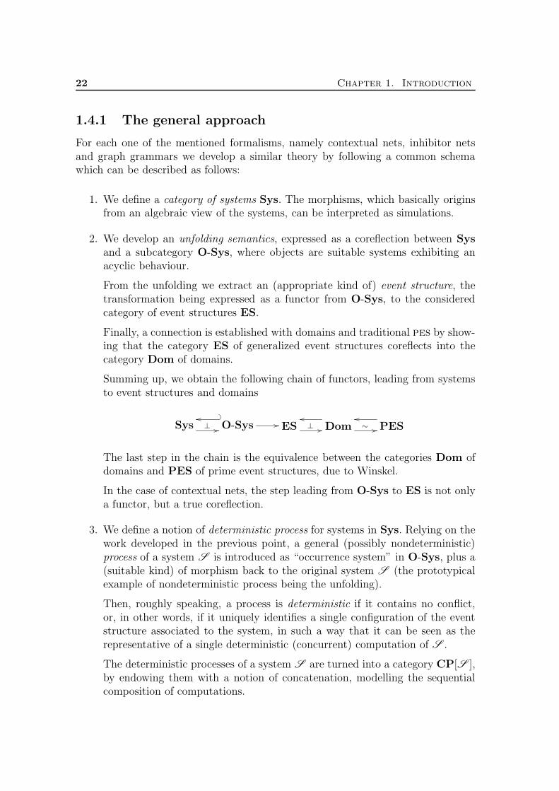
For each one of the mentioned formalisms, namely contextual nets, inhibitor netsand graph grammars we develop a similar theory by following a common schemawhich can be described as follows:
1. We define a category of systems Sys. The morphisms, which basically originsfrom an algebraic view of the systems, can be interpreted as simulations.
2. We develop an unfolding semantics, expressed as a coreflection between Sysand a subcategory O-Sys, where objects are suitable systems exhibiting anacyclic behaviour.
From the unfolding we extract an (appropriate kind of) event structure, thetransformation being expressed as a functor from O-Sys, to the consideredcategory of event structures ES.
Finally, a connection is established with domains and traditional pes by show-ing that the category ES of generalized event structures coreflects into thecategory Dom of domains.
Summing up, we obtain the following chain of functors, leading from systemsto event structures and domains
Sys ⊥ O-Sys ES ⊥ Dom ∼ PES
The last step in the chain is the equivalence between the categories Dom ofdomains and PES of prime event structures, due to Winskel.
In the case of contextual nets, the step leading from O-Sys to ES is not onlya functor, but a true coreflection.
3. We define a notion of deterministic process for systems in Sys. Relying on thework developed in the previous point, a general (possibly nondeterministic)process of a system S is introduced as “occurrence system” in O-Sys, plus a(suitable kind) of morphism back to the original system S (the prototypicalexample of nondeterministic process being the unfolding).
Then, roughly speaking, a process is deterministic if it contains no conflict,or, in other words, if it uniquely identifies a single configuration of the eventstructure associated to the system, in such a way that it can be seen as therepresentative of a single deterministic (concurrent) computation of S .
The deterministic processes of a system S are turned into a category CP[S ],by endowing them with a notion of concatenation, modelling the sequentialcomposition of computations.

1.4. From Petri nets to graph grammars: an overview of the thesis 23
4. We show that the deterministic process and the unfolding semantics canbe reconciled by proving that, as for traditional nets, the comma category〈Initial State ↓ CP[S ]〉, is a preorder whose ideal completion is isomorphicto the domain obtained from the unfolding, as defined at point (2).
1.4.2 Summary of the results
The main achievement of the thesis is the development of a systematic theory ofconcurrency for graph grammars which contribute to close the gap existing betweengraph transformation systems and Petri nets.
1. We define a Winskel’s style semantics for graph grammars. An unfolding con-struction is presented, which associates to each graph grammar a nondeter-ministic occurrence grammar describing its behaviour. Such a constructionestablishes a coreflection between suitable categories of grammars and thecategory of occurrence grammars. The unfolding is then abstracted to an in-hibitor event structure and finally to a prime algebraic domain (or equivalentlyto a prime event structure).
2. We introduce a notion of nondeterministic graph process generalizing the de-terministic processes of [CMR96]. The notion fits nicely in our theory since agraph process of a grammar G can be defined simply as a (special kind of)grammar morphism from an occurrence grammar into G (while in [CMR96]an ad hoc mapping was used).
3. We define concatenable graph processes, as a variation of (deterministic finite)processes endowed with an operation of concatenation, consistent with theflow of causality, which models sequential composition of computations.
The appropriateness of this notion is confirmed by the fact that the categoryCP[G ] of concatenable processes of a grammar G turns out to be isomorphicto the classical truly concurrent model of computation of a grammar based ontraces of [CMR+97, BCE+99].
4. The event structure obtained via the unfolding is shown to coincide both withthe one defined by Corradini et al. [CEL+96b] via a comma category con-struction on the category of concatenable derivation traces, and with the oneproposed by Schied [Sch94], based on a deterministic variant of the dpo ap-proach. These results, besides confirming the appropriateness of the proposedunfolding construction, give an unified view of the various event structuresemantics for the dpo approach to graph transformation.
A second achievement is the development of an analogous unifying theory for twowidely diffused generalizations of Petri nets, namely contextual nets and inhibitornets. While a theory of deterministic processes for these kind of nets was already

24 Chapter 1. Introduction
available in the literature, the Winskel-style semantics, comprising the unfoldingconstruction, its abstraction to a prime algebraic semantics, as well as its relationwith the deterministic process semantics are original.
Finally, we like to mention as a result also the development of a categorical theoryof two kind of generalized event structures, namely asymmetric event structuresand inhibitor event structures and of their relation with Winskel’s event structures.In this thesis they are presented as a mean for the treatment of (extended netsand) grammars, but the generality of the phenomena they allow to model and theirconnections with other extensions of event structures in the literature makes usconvinced that their applicability goes beyond the considered examples.
1.5 Structure of the thesis
The thesis is divided into two parts. The First Part is devoted to the study ofcontextual and inhibitor nets, while the Second Part, exploiting also some notionsand results from the First Part, concentrates on the theory of concurrency of dpograph transformation systems.
The First Part consists of three chapters. In Chapter 2 we introduce somebackground material. After fixing the basic mathematical notation, we present thenotions of contextual and inhibitor net and we review some concurrent semanticsproposed in the literature for these generalized kinds of nets. Then we present thework of Winskel on prime event structures, their equivalence with prime algebraicdomains and we present some generalizations of the basic notion of event structureproposed in the literature.
Chapters 3 and 4 contain the original contributions of the First Part. Chap-ter 3 proposes a truly concurrent semantics for (semi-weighted) contextual netsby following the general approach described in the Introduction. First, we defineasymmetric event structures (aes’s) as a new event based model capable to representthe dependencies between events in contextual net computations and we study theirrelationship with pes’s and domains. Then, exploiting an unfolding construction,the semantics of semi-weighted contextual nets is given via a chain of coreflectionsleading from the category of semi-weighted contextual nets to the category of primealgebraic domains. Finally, we prove that the unfolding and the (deterministic) pro-cess semantics of contextual nets can be reconciled by showing that concatenableprocesses allow to give an alternative characterization of the domain obtained fromthe unfolding.
Chapter 4 generalizes (part of) the work in the previous chapter to the caseof inhibitor nets. This chapter has the same structure as the previous one. First, inorder to deal with the greater complexity of inhibitor net computations we introducea generalization of asymmetric event structures, called inhibitor event structures(ies’s) and we study their relationship with pes’s and domains. Then we give a truly

1.5. Structure of the thesis 25
concurrent semantics for (semi-weighted) inhibitor nets via functorial constructionwhich first associates to each inhibitor net an occurrence inhibitor net. The unfoldingis mapped to an inhibitor event structure and then to a prime algebraic domain.Finally we discuss the notion of deterministic process for inhibitor nets arising fromour theory, we define their concatenable version and we show that, as for contextualnets, concatenable processes allow us to recover the domain semantics of an inhibitornet as obtained via the unfolding construction.
The second part is divided into four chapters. Chapter 5 provides an introduc-tion to the algebraic approach to graph transformation based on the double-pushout(dpo) construction, by presenting some (partly revisited) background notions. Wefirst give the basic definitions of dpo graph grammar, rewriting step and deriva-tion. Then we introduce the fundamental notions of the concurrency theory of thedpo approach by presenting the trace semantics based on the shift equivalence. Thechapter is closed by the definition of the category of graph grammars considered inthis thesis.
The original contributions of the Second Part are presented in Chapters 6-8.Chapter 6 defines an unfolding semantics for dpo graph transformation systems.As for inhibitor nets, the unfolding construction is characterized as a categoricalcoreflection. Then we define a functorial construction which maps the unfolding toan inhibitor event structure, and finally, by the results in Chapter 4, to a primealgebraic domain. This chapter uses many notions and intuitions from Chapter 4on inhibitor nets (in particular it resorts to inhibitor event structures and to theirrelationship with domains).
Chapter 7 presents the notion of concatenable process for dpo graph transfor-mation systems, and proves that the category of concatenable processes provides asemantics for a graph grammar which is equivalent to the classical abstract trulymodel of computation, discussed in Chapter 5. We also study the relationshipbetween the process and the unfolding semantics of a graph grammar, by showing,that, as for nets, concatenable graph processes allow to recover the same domainsemantics defined in Chapter 6.
Chapter 8 reviews two other event structure semantics which have been pro-posed in the literature for dpo graph transformation systems in [CEL+96b, Sch94].By exploiting the results in Chapters 6 and 7, these two alternative event struc-tures are shown to coincide with the one obtained from the unfolding, which thuscan be claimed to be “the” event structure semantics of dpo graph transformation.
Both the First Part and the Second Part end with a summary of the pre-sented results and some final remarks. The Conclusions contains a general dis-cussion on the thesis and sketches possible future directions of research.
Finally, the Appendix collects some basic notions of category theory which areused in the thesis.

26 Chapter 1. Introduction
Origins of the chapters
The truly concurrent semantics for contextual nets presented in Chapter 3 first ap-peared as [BCM98b], while a complete version, including full proofs and the relationwith the process semantics, appeared in [BCM99a].
The notion of nondeterministic process and the unfolding construction for graphtransformation systems described in Chapter 6 can be found in [BCM99b]. Thecharacterization of the unfolding as a universal construction, in the case of semi-weighted grammars, will appear as [BCM99c].
Concatenable graph processes and their relation with the derivation trace se-mantics, presented in Chapter 7, appeared in [BCM98a, BCE+99]. The relationbetween the process and the unfolding semantics, with a different proof, has beenpresented in [BCM99b].
Finally, Chapter 8 relating our event structure semantics with other proposalin the literature has been extracted from [BCM99b].

Part I
Contextual and inhibitor nets


Chapter 2
Background
This chapter presents some background material which will be used in the FirstPart. We first fix the basic mathematical notation. Then we present contextual andinhibitor nets and we review some concurrent semantics proposed in the literaturefor these generalized kinds of nets. In the last part of the chapter we review thework by Winskel on prime event structures, their equivalence with prime algebraicdomains and we present some generalizations of the basic notion of event structureproposed in the literature.
2.1 Basic notation
This section introduces the basic mathematical concepts and notation which areused in the rest of the thesis. It is mainly intended to provide a list of symbolsand keywords with the aim of fixing the notation for sets, relations, functions andmultirelations.
Sets
Without referring to a formal set-theory, we resort to the intuitive notion of set asunordered collection of elements and we use the common operations on sets. Forinstance, given two sets X and X ′ we can consider their union X ∪X ′, intersectionX ∩X ′, difference X −X ′, cartesian product X ×X ′, etc. The cardinality of a setX is denoted by |X|.
The powerset of a set X is denoted by 2X , while 2Xfin denotes the set of finitesubsets of X and 2X1 the set of subsets of X of cardinality at most one (singletonsand the empty set ∅). When Y ∈ 2Xfin we will write Y ⊆fin X. Given a set of setsY ⊆ 2X , the big union of Y is defined as
⋃Y = y | ∃Z ∈ Y. y ∈ Z
and similarly the big intersection of Y is the set⋂Y = y | ∀Z ∈ Y. y ∈ Z. If the

30 Chapter 2. Background
set Y is indexed, i.e., Y = Zi : i ∈ I, its big union and intersection are written as⋃i∈I Zi and
⋂i∈I Zi, respectively.
Relations
Let X and Y be sets. A (binary) relation r from X to Y is a subset of the cartesianproduct of X and Y , namely r ⊆ X × Y . We often use the “infix” and “prefix”notation for relations by writing x r y and r(x, y), respectively, in place of (x, y) ∈ r.We denote by r−1 the inverse relation of r, namely (y, x) | (x, y) ∈ r. The domaindom(r) and codomain cod(r) of the relation r are defined by
dom(r) = x ∈ X | ∃y ∈ Y.(x, y) ∈ r cod(r) = y ∈ Y | ∃x ∈ X.(x, y) ∈ r.
Given X ′ ⊆ X we sometimes write r(X ′) for the set y | ∃x ∈ X. (x, y) ∈ r, calledthe image of X ′ through r.
The composition of two relations r1 ⊆ X × Y and r2 ⊆ Y × Z is the relationr2 r1 ⊆ X × Z, sometimes written r1; r2, defined as follows
r2 r1 = (x, z) | ∃y ∈ Y. (x, y) ∈ r1 ∧ (y, z) ∈ r2
Let us turn our attention to relations r ⊆ X×X (which we call binary relationsover X). By r+ we denote the transitive closure of r, and by r∗ the reflexive andtransitive closure of r. Given X ′ ⊆ X the symbol rX′ indicates the restriction of rto X ′ ×X ′, i.e., r ∩ (X ′ ×X ′).
We say that r is acyclic if it has no “cycles” e0 r e1 r . . . r en r e0, with ei ∈ X,or, in other words, if r+ is irreflexive. We call r well-founded if it has no infinitedescending chains, i.e., eii∈N ∈ X such that ei+1 r ei, ei 6= ei+1, for all i ∈ N. Inparticular, if r is well-founded it has no (non-trivial) cycles.
The relation r is called a preorder if it is reflexive and transitive; it is a partialorder if it is also antisymmetric. The relation r is an equivalence if it is reflexive,transitive and symmetric.
Functions
A partial function f : X → Y is a special relation f ⊆ X×Y with the property thatfor any x ∈ X there is at most one y ∈ Y such that (x, y) ∈ f , namely |f(x)| ≤ 1.In this case we write f(x) = y instead of f(x) = y. Furthermore we writef(x) = ⊥ and we say that f is undefined on x when x 6∈ dom(f), or equivalently iff(x) = ∅. A function f : X → Y is called total if dom(f) = X.
Multisets and Multirelations
Let A be a set. A multiset of A is a function M : A→ N. Such a multiset is denotedsometimes as a formal sumM =
∑a∈A na ·a, where na = M(a). The coefficients 1 are
2.1. Basic notation 31
usually implicit and terms with a zero coefficient are omitted. The set of multisetsof A is denoted by µA.
The usual operations and relations on multisets are used. For instance, multisetunion is denoted by + and defined as (M + M ′)(a) = M(a) + M ′(a); multisetdifference (M −M ′) is defined as (M −M ′)(a) = M(a) −M ′(a) if M(a) ≥ M ′(a)and (M − M ′)(a) = 0 otherwise. We write M ≤ M ′ if M(a) ≤ M ′(a) for alla ∈ A. If M is a multiset of A, we denote by [[M ]] the flattening of M , namelythe multiset
∑a∈A|M(a)>0 1 · a, obtained by changing all non-zero coefficients of
M to 1. Sometimes we confuse the multiset [[M ]] with the corresponding subseta ∈ A |M(a) > 0 of A, and use on them the usual set operations and relations.
A multirelation f : A→ B is a multiset of A× B. It induces in an obvious waya function µf : µA→ µB, defined as
µf(∑
a∈A
na · a) =∑
b∈B
∑
a∈A
(na · f(a, b)) · b.
If the multirelation f satisfies f(a, b) ≤ 1 for all a ∈ A and b ∈ B then we sometimesconfuse it with the corresponding set-relation and write a f b or f(a, b) for f(a, b) =1. We call inverse of f the multirelation f−1 : B → A, defined by f−1(b, a) = f(a, b)for all a ∈ A, b ∈ B.
A multirelation f : A → B is called finitary if for any a in A the set b ∈ B |f(a, b) > 0 is finite. In the following we will consider only finitary multirelations,and thus the qualification “finitary” will be often omitted.
The composition of two multirelations f : A → B and g : B → C is themultirelation g f : A→ C defined as
(g f)(a, c) =∑
b∈B
f(a, b) · g(b, c).
Observe that the above definition is well given only if the involved multirelationsare finitary (since “infinite” coefficients are not allowed). The category having setsas objects and (finitary) multirelations as arrows is denoted by MSet.
We conclude by recalling some trivial properties of multisets which will be usedin the sequel.
Proposition 2.1Let h : A→ B be a multirelation and let M,M ′ ∈ µA. Then
1. µh(M +M ′) = µh(M) + µh(M ′);
2. if M ≤M ′ then µh(M) ≤ µh(M ′);
3. [[µh(M)]] ≤ µh([[M ]]), for all M ∈ µA.

32 Chapter 2. Background
2.2 Contextual and inhibitor nets
In this section we review the definition of contextual and inhibitor nets, the twogeneralizations of ordinary Petri nets which are investigated in the First Part.The adopted notions of concurrent enabling and step sequence (token game) arecompared with other proposals in the literature.
2.2.1 Contextual nets
Contextual nets extend ordinary Petri nets with the possibility of handling contexts:in a contextual net transitions can have not only preconditions and postconditions,but also context conditions. A transition can fire if enough tokens are present inits preconditions and context conditions. In the firing, preconditions are consumed,context conditions remain unchanged and new tokens are generated in the postcondi-tions. We next introduce (marked) contextual P/T nets [Ris94, Bus98] (or c-nets forshort), that following the lines suggested in [MR95] for C/E systems, add contextsto P/T Petri nets.
Definition 2.2 (c-net)A (marked) contextual Petri net (c-net) is a tuple N = 〈S, T, F, C,m〉, where
• S is a set of places;
• T is a set of transitions;
• F = 〈Fpre, Fpost〉 is a pair of multirelations, from T to S.
• C is a multirelation from T to S, called the context relation;
• m is a multiset of S, called the initial marking.
We assume, without loss of generality, that S∩T = ∅. Moreover, we require that foreach transition t ∈ T , there exists at least a place s ∈ S such that Fpre(t, s) > 0.1
This is a common assumption when one is interested in having a causal semanticsfor nets. In fact given a transition with empty pre-set, an unbounded number of in-distinguishable occurrences of such transition can be fired in parallel. Consequently,although a theory of deterministic processes could be still developed, very seriousproblems arise when trying to define an unfolding and an event structure semantics,where each event is intended to represent a uniquely determined occurrence of atransition.
1This is a weak version of the condition of T-restrictedness that requires also Fpost(t, s) > 0,for some s ∈ S.

2.2. Contextual and inhibitor nets 33
Definition 2.3 (pre-set, post-set, and context)Let N be a c-net. As usual, the functions from µT to µS induced by the multirelationsFpre and Fpost are denoted by •( ) and ( )•, respectively. If A ∈ µT is a multiset oftransitions, •A is called its pre-set, while A• is called its post-set. Moreover, by Awe denote the context of A, defined as A = µC(A).
An analogous notation is used to denote the functions from S to 2T definedas, for s ∈ S, •s = t ∈ T | Fpost(t, s) > 0, s• = t ∈ T | Fpre(t, s) > 0,s = t ∈ T | C(t, s) > 0.
For a multiset of transitions A to be enabled by a marking M it is sufficient thatM contains the pre-set of A and at least one additional token in each place in thecontext of A. This corresponds to the intuition that a token in a place can be usedas context by many transitions at the same time and with multiplicity greater thanone by the same transition.
Definition 2.4 (token game)Let N be a c-net and let M be a marking of N , that is a multiset M ∈ µS. Given afinite multiset of transitions A ∈ µT , we say that A is enabled by M if •A+[[A]] ≤M .The transition relation between markings is defined as
M [A〉M ′ iff A is enabled by M and M ′ = M − •A+ A•.
We call M [A〉M ′ a step. A simple step (also called a firing) is a step involving justone transition, i.e., M [t〉M ′.
Definition 2.5 (reachable marking)Let N be a c-net. A marking M is called reachable if there exists a finite stepsequence
m [A0〉M1 [A1〉M2 . . . [An〉M
starting from the initial marking and leading to M .
2.2.2 Inhibitor nets
Inhibitor nets (or nets with inhibitor arcs) further generalize contextual nets withthe possibility of checking not only for the presence, but also for the absence oftokens in a place. Concretely, inhibitor nets are contextual nets enriched with a newrelation that specifies, for each transition, which are the places that inhibit its firing.
Definition 2.6 (i-net)A (marked) inhibitor Petri net (i-net) is a tuple N = 〈S, T, F, C, I,m〉, where〈S, T, F, C,m〉 is a contextual net and I ⊆ T × S is a relation, called the inhibitorrelation.

34 Chapter 2. Background
Let N be an i-net. The pre-set, post-set and context of transitions and places aredefined as for c-nets. Furthermore, for a multiset of transitions A ∈ µT we define theinhibitor set of A, denoted by A, as the set of places which inhibit the transitionsin A, namely A = I([[A]]). Similarly, for a place s we define s = t ∈ T | I(t, s).
The notion of enabling changes in order to take into account also the effect ofthe inhibitor arcs. As for c-nets, a finite multiset of transitions A is enabled by amarking M , if M contains the pre-set of A and covers the context of A. In additionno token must be present nor produced by the step in the places of the inhibitor setof A.
Definition 2.7 (token game)Let N be an i-net and let M ∈ µS be a marking of N . Given a finite multisetof transitions A ∈ µT , we say that A is enabled by M if •A + [[A]] ≤ M and[[M + A•]] ∩ A = ∅. The transition relation between markings is defined as
M [A〉M ′ iff A is enabled by M and M ′ = M − •A+ A•.
Steps, firings and reachable markings are defined in the obvious way.
2.2.3 Alternative approaches
In the literature there is not a complete agreement on the notion of enabling fortransitions and steps of contextual and inhibitor nets. The alternative proposals, forinstance in [Vog97b] and in [JK95], allow for the execution of steps where the sametoken is used both as context and as precondition, or dually of steps where a tokenis generated in the inhibitor set.
The basic assumption which motivates our choice is that concurrent transitionsshould be allowed to fire also in any order. In other words we require that given twomultisets of transitions A1, A2 ∈ µT , then
M [A1 + A2〉M′ ⇒ M [A1〉M
′′ [A2〉M′ for some M ′′.
Consequently, any marking reachable via step sequences is also reachable by firingsequences where each step consists of a single transition.
Without getting into technical details, let us compare the different approaches bymeans of simple examples. Consider the c-nets N0 and N1 in Figure 2.1. Accordingto our definition, the step consisting of the concurrent execution of t0 and t1 is notlegal for both nets.
The definition of [Vog97b] allows for the concurrent execution of t0 and t1 in N0
but not in N1, the idea being that the firings are not instantaneous and two actionsshould be considered concurrent if their executions can overlap in time. This is thecase for t0 and t1 in N0, where the only constraint is that the firing of t0 must startafter the firing of t1 has begun. Instead, in N1 when the firing of a transition startsthe other transition is no more executable. The property that any firing sequence

2.3. Process semantics of generalized Petri nets 35
• •
t0 t1
• •
t0 t1
N0 N1
Figure 2.1: Different notions of enabling in the literature.
serializing a concurrent step must be admissible is weakened to the existence of apossible serialization. Consequently it is still true that the markings reachable viastep sequences coincide with the markings reachable via firing sequences. Accordingto [JK95], instead, the concurrent execution of t0 and t1 is permitted also in N1.Observe that the firing of one of t0 or t1 inhibits the other transition. Hence alsothe weaker property of coincidence of the markings reachable via step and firingsequences is lost.
As already pointed out in [MR95, JK95] the more liberal definitions of enablingare suited to deal with timed systems, where action have non-zero durations, whileour approach is more appropriate when the firings are considered as instantaneous.
We conclude by observing that minor differences exist also with respectto [Bus98], where a single transition is allowed to produce a token in its inhibitor setand the context is a set (rather than a multiset). As for the first point, since in bothapproaches a transition cannot use the same token as precondition and context, wejudge more coherent to forbid the firing also in the dual situation. Moreover, in thisway a multiset of transitions can be safely thought of as a single “composed” tran-sition, making the treatment more uniform. Instead, the choice of viewing contextsas multisets, allowing the firing when at least one token is present in each contextplace, is taken by analogy with graph grammars: a graph production may specify acontext with multiple occurrences of the same resource, but it can be applied witha match which is non-injective on the context. Anyway both choices are mainly amatter of taste, and they have little influence on the developed theory
2.3 Process semantics of generalized Petri nets
The problem of providing a (deterministic) process semantics for contextual andinhibitor nets has been faced by various authors [Vog97b, Ris94, GM98, Win98,Bus98, JK95]. This section is aimed at giving some pointers to the related literatureand an overview of the approaches in [Ris94, GM98, Win98, Bus98] which will be“rediscovered” in the next chapters as special cases of the developed theory. Rather

36 Chapter 2. Background
than giving a formal introduction, the section is intended to explain the frameworkin which our results have been developed.
2.3.1 Contextual nets
A theory of non-sequential processes for contextual nets has been first proposedin [MR95], where two kind of processes for C/E contextual nets are defined. A c-process consists of an ordinary occurrence net with a suitable mapping to the givencontextual net. A simpler notion, called cc-process is obtained by allowing for thepresence of contexts in the occurrence net underlying the process. Contextual P/Tnets and a corresponding notion of deterministic process can be found in the PhDthesis [Ris94] and in [GM98, Win98].
The causal dependency relation for a contextual net N is obtained as the tran-sitive and reflexive closure of the relation ≺N , defined as t ≺N t′ iff
t• ∩ ( •t′ ∪ t′) 6= ∅ ∨ t ∩ •t′ 6= ∅. (†)
A (deterministic) occurrence contextual net is defined as a c-net O where ≺N isirreflexive, the causal dependency relation is a partial order and each place is inthe pre- and post-set of at most one transition. Then, a (deterministic) process ofa c-net N is a deterministic occurrence c-net O, with a total mapping ϕ : O → Npreserving the pre-set, post-set and the context of transitions.
Observe that since an occurrence net is intended to represent a deterministiccomputation, the problem described in the Introduction, related to the presenceof asymmetric conflicts in c-nets does not arise here. Simply, as expressed by (†)above, if t∩ •t′ 6= ∅ then transition t must precede t′ in the computation representedby the net, exactly as it happens for causality, and thus the kind of dependencybetween t and t′ can be safely assimilated to causality.
The papers [GM98, Win98] extend the theory of concatenable processes of ordi-nary nets [DMM89] to c-nets, by showing that the concatenable processes of a c-netN form the arrows of a symmetric monoidal category CP[N ], where the objectsare the elements of the free commutative monoid over the set of places (multisets ofplaces). In particular, in [GM98] a purely algebraic characterization of such categoryis given.
A different approach to the process semantics of contextual nets is consideredin [Vog97b]. As explained before, there the author assumes a different notion ofenabling, allowing for the concurrent firing of two transitions also if one consumes atoken read by the other. Therefore “syntactically” the processes of [Vog97b] coincidewith those in [MR95], but they are intended to represent different step sequences.The paper argues that a partial order is not sufficient to express the dependenciesbetween transitions occurrences even inside a deterministic computation. Thus aprocess is associated with a relational structure consisting of two relations modellingcausality and start precedence (spc-structure) and it is shown that they allow torecover exactly the concurrent computations represented by the process.

2.4. Event structures and domains 37
2.3.2 Inhibitor nets
The deterministic processes of [MR95, Ris94] are generalized to nets with read andinhibitor arcs in [BP96, Bus98, BP99]. An occurrence i-net is naturally defined asan acyclic i-net where all transitions may fire. The main problem in this case is thatthe informations contained in an occurrence i-net may not be sufficient to single outa unique deterministic computation. Consider the simple net below.
•
• t′
t s
t0
As already discussed, there are two possible different executions of the net andthey cannot be reasonably identified from the point of view of causality. To get rid ofthis ambiguity the occurrence i-net underlying a process is enriched by partitioningthe inhibitor arcs in two disjoint sets: the “before” arcs Ib and the “after” arcs Ia.Intuitively, if (t, s) ∈ Ib is a “before” arc then t must be executed before the place sis filled, while if (t, s) ∈ Ia is an “after” arc then t must be executed after the places has been emptied.
Processes of i-nets are shown to be appropriate, in the sense that they uniquelydetermine the causal dependencies among their events, independent transitions canfire concurrently and concurrent sets of places correspond to reachable markings.
A notion of process for elementary net systems (a kind of C/E nets) extendedwith inhibitor arcs is proposed also in [JK95, JK93, JK91]. This work relies onthe more liberal notion of enabling discussed in the previous section, which per-mits the concurrent firing of non serializable transitions. As it happens for c-netsin [Vog97b], this choice makes partial orders insufficient to express the dependenciesbetween events also in a single deterministic computation. To overcome the problemthe authors introduce stratified order structures, where two different relations areemployed to represent causality and weak causality, and weak dependent events mayalso happen simultaneously.
2.4 Event structures and domains
Event structures [NPW81, Win87a] are a widely used model of concurrent compu-tations which arose from the attempt of developing a theory of concurrency incor-porating both the insights of C.A. Petri and D.S. Scott. In this section we introducethe fundamental notions of prime event structure and of prime algebraic domain,and we review the close relationship between these mathematical models explaininghow they can be seen as equivalent presentations of the same fundamental idea.

38 Chapter 2. Background
Finally we review some generalizations of prime event structures which have beenproposed in the literature to overcome some limitations of expressiveness of primeevent structures.
2.4.1 Prime event structures
Prime event structures (pes) [NPW81] are a simple event-based model of concurrentcomputations in which events are considered as atomic and instantaneous steps,which can appear only once in a computation. An event can occur only after someother events (its causes) have taken place and the execution of an event can inhibitthe execution of other events. This is formalized via two binary relations: causality,modelled by a partial order relation ≤ and conflict, modelled by a symmetric andirreflexive relation #, hereditary with respect to causality.
Definition 2.8 (prime event structures)A prime event structure (pes) is a tuple P = 〈E,≤,#〉, where E is a set of eventsand ≤, # are binary relations on E called causality relation and conflict relationrespectively, such that:
1. the relation ≤ is a partial order and ⌊e⌋ = e′ ∈ E : e′ ≤ e is finite for alle ∈ E;
2. the relation # is irreflexive, symmetric and hereditary with respect to ≤, i.e.,e#e′ ≤ e′′ implies e#e′′ for all e, e′, e′′ ∈ E;
A configuration of a pes is a set of events representing a possible computationof the system modelled by the event structure.
Definition 2.9 (configuration)A configuration of a pes P = 〈E,≤,#〉 is a subset of events C ⊆ E such that forall e, e′ ∈ C
1. ¬(e#e′) (conflict-freeness)
2. ⌊e⌋ ⊆ C (left-closedness)
Given two configurations C1 ⊆ C2 if e0, . . . , en is any linearization of the events inC2 − C1, compatible with causality, then
C1 ⊆ C1 ∪ e0 ⊆ C1 ∪ e0, e1 ⊆ . . . ⊆ C2
is a sequence of well-defined configurations. Therefore subset inclusion can be safelythought of as a computational ordering on configurations.
Definition 2.10 (poset of configurations)We denote by Conf (P ) the set of configurations of a prime event structure P , orderedby subset inclusion.

2.4. Event structures and domains 39
The class of pes is turned into a category by introducing a notion of morphism.
Definition 2.11 (category PES)Let P0 = 〈E0,≤0,#0〉 and P1 = 〈E1,≤1,#1〉 be two pes’s. A pes-morphismf : P0 → P1 is a partial function f : E0 → E1 such that:
1. for all e0 ∈ E0, if f(e0) 6= ⊥ then ⌊f(e0)⌋ ⊆ f(⌊e0⌋);
2. for all e0, e′0 ∈ E0, if f(e0) 6= ⊥ 6= f(e′0) then
(a) (f(e0) = f(e′0)) ∧ (e0 6= e′0) ⇒ e0#0e′0;
(b) f(e0)#1f(e′0) ⇒ e0#0e′0;
The category of prime event structures and pes-morphisms is denoted by PES.
It is possible to verify that pes morphisms “preserve computations”, in the sense thatthe image through a pes morphism of a configuration is a configuration. Thereforea pes morphism naturally induces a monotone mapping between the correspondingposets of configurations.
2.4.2 Prime algebraic domains
This subsection reviews the definition of the category Dom of finitary prime alge-braic domains as introduced in [Win87a]. The intuition behind their computationalinterpretation helps in understanding the close relationship existing between do-mains and event structures, which can be formalized, at categorical level, as anequivalence of categories.
First we need some basic notions and notations for partial orders. A preorderedor partially ordered set 〈D,⊑〉 will be often denoted simply as D, by omittingthe (pre)order relation. Given an element x ∈ D, we write ↓ x to denote the sety ∈ D | y ⊑ x. A subset X ⊆ D is compatible, written ↑ X, if there exists anupper bound d ∈ D for X (i.e., x ⊑ d for all x ∈ X). It is pairwise compatible if↑ x, y (often written x ↑ y) for all x, y ∈ X. A subset X ⊆ D is called directed iffor any x, y ∈ X there exists z ∈ X such that x ⊑ z and y ⊑ z.
Definition 2.12 ((finitary) (algebraic) complete partial order)A partial order D is (directed) complete (cpo) if for any directed subset X ⊆ Dthere exists the least upper bound
⊔X in D. An element e ∈ D is compact if for any
directed set X ⊆ D, e ⊑⊔X implies e ⊑ x for some x ∈ X. The set of compact
elements of D is denoted by K(D).A cpo D is called algebraic if for any x ∈ D, x =
⊔(↓ x ∩ K(D)). We say that
D is finitary if for each compact element e ∈ D the set ↓ e is finite.
Given a finitary algebraic cpo D we can think of its elements as “pieces of informa-tion” expressing the states of evolution of a process. Finite elements represent states

40 Chapter 2. Background
which are reached after a finite number of steps. Thus algebraicity essentially saysthat each infinite computation can be approximated with arbitrary precision by thefinite ones.
Winskel’s domains satisfy stronger completeness properties, which are formalizedby the following definition.
Definition 2.13 ((prime algebraic) coherent poset)A partial order D is called coherent (pairwise complete) if for all pairwise compatibleX ⊆ D, there exists the least upper bound
⊔X of X in D.
A complete prime of D is an element p ∈ D such that, for any compatibleX ⊆ D, if p ⊑
⊔X then p ⊑ x for some x ∈ X. The set of complete primes of D is
denoted by Pr(D). The partial order D is called prime algebraic if for any elementd ∈ D we have d = (
⊔↓ d ∩ Pr(D)). The set ↓ d ∩ Pr(D) of complete primes of D
below d will be denoted Pr(d).
Being not expressible as the least upper bound of other elements, the completeprimes ofD can be seen as elementary indivisible pieces of information (events). Thusprime algebraicity expresses the fact that all the possible computations of the systemat hand can be obtained by composing these elementary blocks of information.
Notice that directed sets are pairwise compatible, and thus each coherent partialorder is a cpo. For the same reason each complete prime is a compact element,namely Pr(D) ⊆ K(D) and thus prime algebraicity implies algebraicity. Moreover ifD is coherent then for each non empty X ⊆ D there exists the greatest lower bounddX, which can be expressed as
⊔y ∈ D | ∀x ∈ X. y ⊑ x.
Definition 2.14 (domains)The partial orders we shall work with are coherent, prime algebraic, finitary partialorders, hereinafter simply referred to as (Winskel’s) domains.2
The definition of morphism between domains is based on the notion of immediateprecedence. Given a domain D and two distinct elements d 6= d′ ∈ D we say that dis an immediate predecessor of d′, written d ≺ d′ if
d ⊑ d′ ∧ ∀d′′ ∈ D. (d ⊑ d′′ ⊑ d′ ⇒ d′′ = d ∨ d′′ = d′)
Moreover we write d d′ if d ≺ d′ or d = d′. According to the informal interpretationof domain elements sketched above, d d′ intuitively means that d′ is obtained fromd by adding a quantum of information. Domain morphisms are required to preservesuch relation.
2The use of this kind of structures in semantics have been first investigated by Berry [Ber78],where they are called dI-domains. The relation between Winskel domains and dI-domains, which arefinitary distributive consistent-complete algebraic cpo’s is established by the fact that for a finitaryalgebraic consistent-complete (or coherent) cpo, prime algebraicity is equivalent to distributivity.

2.4. Event structures and domains 41
Definition 2.15 (category Dom)Let D0 and D1 be domains. A domain morphism f : D0 → D1 is a function, suchthat:
• ∀x, y ∈ D0, if x y then f(x) f(y). (-preserving)
• ∀X ⊆ D0, X pairwise compatible, f(⊔X) =
⊔f(X); (Additive)
• ∀X ⊆ D0, X 6= ∅ and compatible, f(dX) =
df(X); (Stable)
We denote by Dom the category having domains as objects and domain morphismsas arrows.
Relating prime event structures and domains
Both event structures and domains can be seen as models of systems where com-putations are built out from atomic pieces. Formalizing this intuition, in [Win87a]the category Dom is shown to be equivalent to the category PES, the equivalencebeing established by two functors L : PES→ Dom and P : Dom→ PES
PESL
∼ DomP
The functor L associates to each pes the poset Conf (P ) of its configurationswhich can be shown to be a domain. The image via L of a pes-morphism f : P0 →P1 is the obvious extension of f to sets of events.
The definition of the functor P, mapping domains back to pes’s requires theintroduction of the notion of prime interval.
Definition 2.16 (prime interval)Let 〈D,⊑〉 be a domain. A prime interval is a pair [d, d′] of elements of D such thatd ≺ d′. Let us define
[c, c′] ≤ [d, d′] if (c = c′ ⊓ d) ∧ (c′ ⊔ d = d′),
and let ∼ be the equivalence obtained as the transitive and symmetric closure of (thepreorder) ≤.
The intuition that a prime interval represents a pair of elements differing only for a“quantum” of information is confirmed by the fact that there exists a bijective cor-respondence between ∼-classes of prime intervals and complete primes of a domainD (see [NPW81]). More precisely, the map
[d, d′]∼ 7→ p,
where p is the unique element in Pr(d′)−Pr(d), is an isomorphism between the ∼-classes of prime intervals of D and the complete primes Pr(D) of D, whose inverseis the function:

42 Chapter 2. Background
p 7→ [⊔c ∈ D | c ⊏ p, p]∼.
The above machinery allows us to give the definition of the functor P “extracting”an event structure from a domain.
Definition 2.17 (from domains to pes’s)The functor P : Dom→ PES is defined as follows:
• given a domain D, P(D) = 〈Pr(D),≤,#〉 where
p ≤ p′ iff p ⊑ p′ and p#p′ iff ¬(p ↑ p′);
• given a domain morphism f : D0 → D1, the morphism P(f) : P(D0) →P(D1) is the function:
P(f)(p0) =
p1 if p0 7→ [d0, d′0]∼, f(d0) ≺ f(d′0)
and [f(d0), f(d′0)]∼ 7→ p1;
⊥ otherwise, i.e., if f(d0) = f(d′0).
2.4.3 Generalized event structure models
To represent in a direct way the behaviour of languages or models of computationswhere the dependencies between events are not adequately described in terms ofcausality and conflict, several extensions of prime event structures have been con-sidered in the literature. Some of these extensions can be seen as special subclassesof the more general Winskel’s event structures, while others represents orthogonalgeneralizations of Winskel’s model.
Flow and bundle event structures
In a prime event structure, and more generally in a stable event structure, each eventhas a uniquely determined history, namely given an event we can always identifya unique subset of events which are necessary for the execution of e, the set of itscauses.
While in certain situations the mentioned property is appreciable since it gives tothe events a very simple operational meaning, in other cases it may be an undesirablerestriction. Consider for instance a process algebra with nondeterministic choice“+”and sequential composition “;” operators. To give a pes semantics of a term(a + b); c we are forced to use two different events to represent the execution of c,one for the execution of c after a and the other for the execution of c after b.
To model nondeterministic choices, or equivalently the possibility of having mul-tiple disjunctive and mutually exclusive causes for an event, Boudol and Castel-lani [BC88] introduce the notion of flow event structure, where the causality relationis replaced by an irreflexive (in general non transitive) flow relation, representingessentially immediate causal dependency, and conflict is no more hereditary.

2.4. Event structures and domains 43
e1 # e2 # e3 # e4 # e5
e
Figure 2.2: A flow event structure F such that there are no bundle event structureswith the same configurations.
Definition 2.18 (flow event structure)A flow event structure is a triple 〈E,≺,#〉, where E is a denumerable set of events,≺⊆ E × E is an irreflexive relation called the flow relation, and # ⊆ E × E is thesymmetric conflict relation.
A configuration is then defined as a conflict free set of events, where the flow relationis acyclic, and given any event e in the configuration, if e′ ≺ e then the configurationmust contain e′ or another event e′′ in conflict with e′ such that e′′ ≺ e (thus one ofthe disjunctive causes must be present in the configuration).
To face a similar problem in the semantics of lotos, Langerak [Lan92a, Lan92b]defines bundle event structures, where a set of multiple disjunctive and mutuallyexclusive causes for an event is called a bundle set for the event, and comes into playas a primitive notion.
Definition 2.19 (bundle event structure)A bundle event structure is a triple 〈E, 7→,#〉, where E is the denumerable set ofevents, # ⊆ E×E is the (irreflexive) symmetric conflict relation and 7→⊆ 2Efin×E isthe bundle relation. Distinct events in the same bundle are required to be in conflict.
The explicit representation of the bundles makes bundle event structures strictly lessexpressive than flow event structures. For instance, consider the flow event structureF in Figure 2.2, where conflict is represented by dotted lines labelled by #, whilethe flow relation is represented by arrows. The configurations of F are e1, e3, e5,e1, e4 and e2, e4. Observing that the only possible bundles are pairs of conflictualevents it is not difficult to see that there are no bundle event structures having thesame set of configurations (see [Lan92b] for a wider discussion). On the other hand,bundle event structures offer the advantage of having a simpler theory. For instance,differently from what happens for flow event structures, non-executable events canbe removed without affecting the behaviour of the event structure.
Event automata and asymmetric conflicts
The papers [PP92, PP95] introduce the “operational” notion of event automaton,which can be seen as a generalization of the set of configurations of an event struc-ture. An event automaton is a triple E = 〈E, St,_〉, where E is a set of events,

44 Chapter 2. Background
St ⊆ 2Efin is a set of states and _⊆ St × St is a relation such that if X _ Y thenthe state Y is obtained from X by adjoining a single event.
A language is introduced which allows one to specify in logical terms the be-haviour of an event automata, and an event structure can then be thought of as aspecification expressed in the language. In particular, including negation in the lan-guage and allowing for prescriptions of the kind “¬e1 ⊢ e0”, meaning that the evente0 is enabled in a state S if e1 6∈ S, one is naturally lead to the notion of possibleevent and asymmetric conflict. In fact, if “¬e1 ⊢ e0” holds then if both events arein the same state, necessarily e0 must have been executed first. Hence, as alreadydiscussed, we can think that e0 is a possible cause of e1, or that an asymmetricconflict exists between the two events.
Inspired by these considerations, the paper [PP95] extends prime and flow eventstructures with possible events/flow. A prime event structure with possible events isa tuple 〈E,Ep,≤,#〉, where 〈E,≤,#〉 is a pes and Ep ⊆ E is a set of possible events.A configuration is then required to contain all the causes of an event in E−Ep, butsome possible causes may be absent.
Similarly, a flow event structure with possible flow is a flow event structure en-riched with a new relation <p, called the possible flow relation. The flow and possibleflow relations must be acyclic on a configuration, but the causal closure is requestedonly with respect to the flow relation. Again the precedences imposed by the possibleflow relation can be thought of as possible precedences.
To conclude, it is worth remarking that similar ideas are developed, under adifferent perspective by Degano, Vigna and Gorrieri, in [DGV93, Bod98], where pri-oritized event structures are introduced as pes enriched with a partial order relationmodelling priorities between events. Furthermore also bundle event structures havebeen extended by Langerak in [Lan92b] to take into account asymmetric conflicts.
Chapter 3
Semantics of Contextual Nets
This chapter presents an event structure semantics for contextual nets, an extensionof P/T Petri nets where transitions can check for the presence of tokens withoutconsuming them (read-only operations). A basic role is played by asymmetric eventstructures, a generalization of Winskel’s prime event structures where symmetricconflict is replaced by a relation modelling asymmetric conflict or weak causality,used to represent the new kind of dependency between events arising in contextualnets. Extending Winskel’s seminal work on safe nets, the truly concurrent eventbased semantics of contextual nets is given at categorical level via a chain of core-flections leading from the category SW-CN of semi-weighted contextual nets to thecategory Dom of finitary prime algebraic domains:
SW-CNUa
⊥ O-CNEa
⊥
IO
AESLa
⊥
Na
DomPa
P
∼ PESL
First an unfolding construction generates from a contextual net N a correspondingoccurrence contextual net Ua(N). The unfolding describes the behaviour of N in astatic way by making explicit the possible events in the computations of the netand the dependency relations between them. The construction can be extended toa functor from SW-CN to the category O-CN of occurrence contextual nets, thatis right adjoint to the inclusion functor. The transitions of an occurrence contextualnet are related by causal dependency and asymmetric conflict, and thus, the seman-tics of semi-weighted contextual nets given in terms of occurrence contextual netscan be naturally abstracted to an aes semantics: given an occurrence contextualnet we obtain an aes simply forgetting the places, but remembering the depen-dency relations that they induce between transitions. Again, this transformation isexpressed, at categorical level, as a coreflection between the category AES of asym-metric event structures and O-CN. Finally, the configurations of the asymmetricevent structure, endowed with a suitable order, are shown to form a finitary primealgebraic domain. This last step generalizes Winskel’s equivalence between PES andDom to the existence of a coreflection between AES and Dom. Such a coreflection

46 Chapter 3. Semantics of Contextual Nets
allows for an elegant translation of the aes semantics into a domain, and thus (viaWinskel’s equivalence) into a traditional pes semantics.
We also investigate the relation between the proposed unfolding semantics andseveral deterministic process semantics for contextual nets in the literature. Firstwe show that the notion of deterministic process naturally arising from our theorycoincides with other common proposals in the literature. Then a tight relationshipis established between the unfolding and the deterministic process semantics, byshowing that the domain obtained via the unfolding can be characterized as thecollection of the deterministic processes of the net endowed with a kind of prefixordering.
The rest of the chapter is organized as follows. Section 3.1 introduces the cat-egory AES of asymmetric event structures and describes some properties of suchstructures. Section 3.2 defines the coreflection between AES and the category Domof finitary prime algebraic domains. Section 3.3 presents the category of contextualnets and focuses on the subcategory SW-CN of (semi-weighted) contextual netswhich we shall work with. Section 3.4 is devoted to the definition and analysis of thecategory O-CN of occurrence contextual nets. Section 3.5 describes the unfoldingconstruction for semi-weighted contextual nets and shows how such a constructiongives rise, at categorical level, to a coreflection between SW-CN and O-CN. Sec-tion 3.6 completes the chain of coreflections from SW-CN to Dom, by presentinga coreflection between O-CN and AES. Section 3.7 discusses the relation betweenthe unfolding and the deterministic process semantics of contextual nets.
3.1 Asymmetric conflicts and asymmetric event
structures
We stressed in the Introduction that pes’s (and in general Winskel’s event struc-tures) are not expressive enough to model in a direct way the behaviour of modelsof computation, such as string, term, graph rewriting and contextual nets, where arule may preserve a part of the state, in the sense that part of the state is necessaryfor the application of the rule, but it is not affected by such application.
The critical situation when dealing with contextual nets is represented by thenet in Figure 3.1.(a), where the firing of t1 inhibits t0, but not vice versa. Thedependency between the two transitions can be seen either as a kind of asymmetricconflict or as a weak form of causality, and cannot be modelled directly via a pes.
A reasonable way to encode this situation in a pes is to represent the firing oft0 with an event e0 and the firing of t1 with two distinct mutually exclusive events:e′1, representing the execution of t1 that prevents t0, thus mutually exclusive withe0; and e′′1, representing the execution of t1 after t0 (thus caused by e0). Such pes isdepicted in Figure 3.1.(b), where causal dependency is represented by a plain arrowand conflict is represented by a dotted line, labelled by #. However, this solution is

3.1. Asymmetric conflicts and asymmetric event structures 47
N0
•s0
t0 •s
t1
e′1 # e0
e′′1
(a) (b)
Figure 3.1: A simple contextual net and a prime event structure representing itsbehaviour.
not completely satisfactory with respect to the interpretation of contexts as “read-only resources”: since t0 just reads the token in s without changing it, one wouldexpect the firing of t1, preceded or not by t0, to be represented by a unique event.This encoding may lead to an explosion of the size of the pes, since whenever anevent is “duplicated” also all its consequences must be duplicated. In addition itshould be noted that the information on the new kind of dependency determinedby read-only operations is completely lost because it is “confused” with causality orsymmetric conflict.
It is worth noting that the inability of representing the asymmetric conflict be-tween events without resorting to duplications is not specific to prime event struc-tures, but it is basically related to the axiom of general Winskel’s event structures(see [Win87a], Definition 1.1.1) stating that the enabling relation ⊢ is “monotone”with respect to set inclusion:
A ⊢ e ∧ A ⊆ B ∧ B consistent ⇒ B ⊢ e.
A consequence of this axiom is that the computational order between configurationsis set inclusion, the idea being that if A and B are finite configurations such asA ⊆ B, then starting from A we can reach B by performing the events in B − A,whenever they become enabled. Obviously, this axiom does not hold in the presenceof asymmetric conflict.
As mentioned in the previous chapter (Section 2.4), the problem of represent-ing asymmetric conflicts in event structures has been already faced in the litera-ture [PP92, Lan92b]. However none of the proposed models is suited for our aims.On the one hand, pes’s with possible events [PP92]are not sufficiently expressivesince they resort to a “global” notion of possible event. For example, the net of Fig-ure 3.2 cannot be modelled by a pes with possible events since transition t0 shouldbe a “possible” cause for t1, but a “strong” cause for t2. On the other hand flow eventstructures with possible flow and bundle event structures with asymmetric conflictare expressive enough, but unnecessarily complicate for our aims due to their possi-bility of expressing multiple disjunctive causes. Technically, as it will become clear

48 Chapter 3. Semantics of Contextual Nets
in the next chapter, this greater generality would have prevented us from realizingthe step from occurrence c-nets to event structures as a coreflection. Furthermore nocategorical treatment of such models was available, and their relation with domainsand pes’s was not fully investigated.
•
t0 •
t1
t2
Figure 3.2: A contextual net for which pes’s with possible events are not adequate.
3.1.1 Asymmetric event structures
In order to provide a more direct, event based representation of the behaviour ofcontextual nets this section introduces a new kind of event structure, called asym-metric event structure (aes). An aes, besides of the usual causal relation ≤ of aprime event structure, has a relation ր that allows us to specify the new kind ofdependency described above for transitions t0 and t1 of the net in Figure 3.1 simplyas t0 ր t1. As already remarked, the same relation has two natural interpretations:it can be thought of either as an asymmetric version of conflict or as a weak formof causality. We decided to call it asymmetric conflict, but the reader should keepin mind both views, since in some situations it will be preferable to refer to theweak causality interpretation. Informally, in an aes each event has a set of “strong”causes (given by the causal dependency relation) and a set of weak causes (due tothe presence of the asymmetric conflict relation). To be fired, each event must bepreceded by all strong causes and by a (suitable) subset of the weak causes. There-fore, differently from pes’s, the firing of an event can have more than one history.However observe that aes’s still satisfy a property of stability, since a least historyalways exists, coinciding with the set of strong causes.
It comes of no surprise that in this setting the symmetric binary conflict is notanymore needed as a primitive relation, but it can be represented via “cycles” ofasymmetric conflict. For instance, if e ր e′ and e′ ր e then clearly e and e′ cannever occur in the same computation. As a consequence, pes’s can be identified witha special subclass of asymmetric event structures, namely those where all conflictsare actually symmetric.

3.1. Asymmetric conflicts and asymmetric event structures 49
The basic ideas for the treatment of asymmetric conflict in our approach aresimilar to those suggested by Pinna and Poigne in [PP92, PP95]. Apart from adifferent presentation, asymmetric event structures can be seen as a generalizationof pes with possible events. Using their terminology, when e0 ր e1 we can saythat e0 is a possible cause of e1. However, differently from what happens for eventstructures with possible events, where a distinct set of possible events is singledout, our notion of possible cause is local, being induced by the asymmetric conflictrelation. The extended bundle event structures of Langerak [Lan92b] share with ourapproach also the intuition that when asymmetric conflict is available, the symmetricconflict becomes useless.
For technical reasons we first introduce pre-asymmetric event structures. Thenasymmetric event structures will be defined as special pre-asymmetric event struc-tures satisfying a suitable condition of “saturation”.
Recall from Section 2.1 that given a relation r ⊆ X × X and a subset Y ⊆ X,we denote by rY the restriction of r to Y , namely r ∩ (Y × Y ).
Definition 3.1 (pre-asymmetric event structure)A pre-asymmetric event structure (pre-aes) is a tuple G = 〈E,≤,ր〉, where E isa set of events and ≤, ր are binary relations on E called causality relation andasymmetric conflict respectively, such that:
1. the relation ≤ is a partial order and ⌊e⌋ = e′ ∈ E | e′ ≤ e is finite for alle ∈ E;
2. the relation ր satisfies, for all e, e′ ∈ E:
(a) e < e′ ⇒ eր e′;1
(b) ր⌊e⌋ is acyclic.2
If eր e′, according to the double interpretation of ր, we say that e is prevented bye′ or e weakly causes e′. Moreover we say that e is strictly prevented by e′ (or thate strictly weakly causes e′), written e e′, if eր e′ and ¬(e < e′).
The definition can be easily understood by giving a more precise account of theideas presented in the Introduction. Let FiredC(e) denote the fact that the evente has been fired in a computation C, later formalized by the notion of configuration,and let precC(e, e′) denote that e precedes e′ in the computation. Then
e < e′ means that ∀C. FiredC(e′) ⇒ FiredC(e) ∧ precC(e, e′)
eր e′ means that ∀C. FiredC(e) ∧ FiredC(e′) ⇒ precC(e, e′).
1With e < e′ we mean e ≤ e and e 6= e′.2Equivalently, we can require (ր⌊e⌋)
+ irreflexive. This implies, in particular, that the relationր is irreflexive.

50 Chapter 3. Semantics of Contextual Nets
e0 e′0
e e′
Figure 3.3: A pre-aes with two conflictual events e and e′, not related by asymmetricconflict.
Therefore < represents a global order of execution, while ր determines an order ofexecution only locally to each computation. Thus it is natural to imposeր to be anextension of <. Moreover notice that if a set of events form a cycle of asymmetricconflict then such events cannot appear in the same computation, otherwise theexecution of each event should precede the execution of the event itself. This explainswhy we require the transitive closure ofր, restricted to the causes ⌊e⌋ of an event e,to be acyclic (and thus well-founded, being ⌊e⌋ finite). Otherwise not all causes of ecould be executed in the same computation and thus e itself could not be executed.The informal interpretation makes also clear that ր is not in general transitive. Ifeր e′ ր e′′ it is not true that e must precede e′′ when both fire. This holds only ina computation where also e′ fires.
The fact that a set of events in a cycle of asymmetric conflict can never occurin the same computation can be naturally interpreted as a kind of conflict. Moreformally, it is useful to associate to each pre-aes an explicit conflict relation (on setsof events) defined in the following way:
Definition 3.2 (induced conflict relation)Let G = 〈E,≤,ր〉 be a pre-aes. The conflict relation #a ⊆ 2Efin associated to G isdefined as:
e0 ր e1 ր . . .ր en ր e0#ae0, e1, . . . , en
#a(A ∪ e) e ≤ e′
#a(A ∪ e′)
where A denotes a generic finite subset of E. The superscript “a” in #a reminds thatthis relation is induced by asymmetric conflict. Sometimes we use the infix notationfor the “binary version” of the conflict, i.e., we write e#ae′ for #ae, e′.
Notice that if #aA then ⌊A⌋ contains a cycle of asymmetric conflict, and, vice versa,if ⌊A⌋ contains a cycle e0 ր e1 . . . en ր e0 then there exists a subset A′ ⊆ A suchthat #aA′ (for instance, by choosing an event ai ∈ A such that ei ≤ ai for eachi ∈ 0, . . . , n the set A′ can be ai | i ∈ 0, . . . , n).
Clearly, by the rules above, if e ր e′ and e′ ր e then #ae, e′. The converse,instead, does not hold, namely in general we can have e#ae′ and ¬(e ր e′), as inthe aes Figure 3.3, because #a is inherited along <, whileր is not. An asymmetric

3.1. Asymmetric conflicts and asymmetric event structures 51
event structure is a pre-aes where each binary conflict is induced directly by anasymmetric conflict in both directions.
Definition 3.3An asymmetric event structure (aes) is a pre-aes G = 〈E,≤,ր〉 such that for anye, e′ ∈ E, if e#ae′ then eր e′.
Observe that given any pre-aes G = 〈E,≤,ր〉, we can always “saturate” G inorder to obtain an aes G = 〈E,≤,ր′〉, by defining ր′ as e ր′ e′ if and only if(eր e′) ∨ (e#ae′). Furthermore it is easy to verify that the conflict relations of Gand of G′ coincide.
3.1.2 Morphisms of asymmetric event structures
The notion of aes-morphism is a quite natural extension of that of pes-morphism.Intuitively, it is a (possibly partial) mapping of events that “preserves computa-tions”.
Definition 3.4 (aes-morphism)Let G0 = 〈E0,≤0,ր0〉 and G1 = 〈E1,≤1,ր1〉 be two aes’s. An aes-morphismf : G0 → G1 is a partial function f : E0 → E1 such that:
1. for all e0 ∈ E0, if f(e0) 6= ⊥ then ⌊f(e0)⌋ ⊆ f(⌊e0⌋);
2. for all e0, e′0 ∈ E0, if f(e0) 6= ⊥ 6= f(e′0) then
(a) (f(e0) = f(e′0)) ∧ (e0 6= e′0) ⇒ e0#a0e′0.
(b) f(e0)ր1 f(e′0) ⇒ e0 ր0 e′0;
It is easy to show that aes-morphisms are closed under composition. In fact, letf0 : G0 → G1 and f1 : G1 → G2 be aes-morphisms. The fact that f1 f0 satisfiesconditions (1) and (2.a) of Definition 3.4 is proved as for ordinary pes’s. The validityof condition (2.b) is straightforward.
Definition 3.5 (category AES)We denote by AES the category having asymmetric event structures as objects andaes-morphisms as arrows.
Notation 3.6In the following when considering a pes P and an aes G, we implicitly assume thatP = 〈E,≤,#〉 and G = 〈E,≤,ր〉. Moreover superscripts and subscripts on thestructure name carry over the names of the involved sets, functions and relations(e.g., Gi = 〈Ei,≤i,րi〉).

52 Chapter 3. Semantics of Contextual Nets
The binary conflict in an aes is represented by asymmetric conflict in bothdirections, and thus, analogously to what happens for pes’s, it is reflected by aes-morphisms. The next lemma shows that aes-morphisms reflect also the general(induced) conflict relation.
Lemma 3.7 (aes-morphisms reflect conflicts)Let G0 and G1 be two aes’s and let f : G0 → G1 be an aes-morphism. Given a setof events A ⊆fin E0, if #a
1f(A) then #a0A′ for some A′ ⊆ A.
Proof. Let A ⊆fin E0 and let #a1f(A). By definition of conflict there is a ր1-cycle e′0 ր1
e′1 ր1 . . .ր1 e′n ր1 e
′0 in ⌊f(A)⌋. By definition of aes-morphism, we have that ⌊f(A)⌋ ⊆ f(⌊A⌋)
and thus we can find e0, . . . , en ∈ ⌊A⌋ such that e′i = f(ei) for all i ∈ 0, . . . , n. ConsiderA′ = a0, . . . , an ⊆ A such that ei ≤0 ai for i ∈ 0, . . . , n. By definition of aes-morphism,e0 ր0 e1 ր0 . . .ր0 e0, and thus #a
0A′. 2
3.1.3 Relating asymmetric and prime event structures
We conclude this section by formalizing the relation between aes’s and pes’s. Weshow that aes’s are a proper extension of pes’s, in the sense that, as one wouldexpect, pes’s can be identified with the subclass of aes’s where the strict asymmetricconflict relation is actually symmetric. The corresponding full embedding functor isright adjoint to the forgetful functor from AES to PES.
Lemma 3.8Let P = 〈E,≤,#〉 be a pes. Then G = 〈E,≤, < ∪#〉 is an aes, where the asym-metric conflict relation is defined as the union of the “strict” causality and conflictrelations.
Moreover, if f : P0 → P1 is a pes-morphism then f is an aes-morphism betweenthe corresponding aes’s G0 and G1, and if g : G0 → G1 is an aes-morphism thenit is also a pes-morphism between the original pes’s.
Proof. Let P = 〈E,≤,#〉 be a pes. The fact that G = 〈E,≤, < ∪#〉 is an aes is a trivialconsequence of the definitions. In particular, the asymmetric conflict relation of G is acyclic onthe causes of each event since # is hereditary with respect to ≤ and irreflexive, and < is a strictpartial order (namely an irreflexive and transitive relation) in P .
Now, let f : P0 → P1 be a pes-morphism. To prove that f is also an aes-morphism between thecorresponding aes’s G0 and G1, first observe that, according the definition of ≤Gi
and րGi, the
validity of the conditions (1) and (2.a) of Definition 3.4 follows immediately from the correspondingconditions in the definition of pes-morphism (Definition 2.11). As for condition (2.b), if f(e0)րG1
f(e1), then, by construction, f(e0) <P1 f(e1) or f(e0)#P1f(e1) and thus, by properties of pes’s(easily derivable from Definition 2.11), in the first case e0 <P0 e1 or e0#P0e1 whilst, in the secondcase, e0#P0e1. Hence, in both cases, e0 րG0 e1.
Similar considerations allow us to conclude that, if g : G0 → G1 is an aes-morphism, then itis also a pes-morphism between the original pes’s. 2

3.2. From asymmetric event structures to domains 53
By the previous lemma, there is a full embedding functor from PES into AESthat transforms each pes by replacing the symmetric conflict with an asymmetricconflict relation given by the union of “strict” causality and conflict relation, andthat is identity on arrows.
Proposition 3.9 (from pes’s to aes’s)The functor J : PES→ AES defined by
• J (〈E,≤,#〉) = 〈E,≤, < ∪#〉;
• J (f : P0 → P1 ) = f
is a full embedding of PES into AES.
Observe that given any aes G = 〈E,≤,ր〉 the induced binary conflict, whichcan be expressed as ր ∩ ր−1, satisfies all the properties of the conflict relation ofpes’s, i.e., it is irreflexive (since ր is irreflexive), symmetric and hereditary withrespect to ≤. Therefore 〈E,≤,#〉, where # =ր ∩ ր−1, is a pes, in the followingreferred to as the pes underlying the aes G.
Definition 3.10 (pes underlying an aes)We denote by Fap : AES → PES the forgetful functor defined on objects asFap(G) = 〈E,≤,ր ∩ ր−1〉 and which is the identity on arrows.
The functor is well-defined, as it can be verified by showing that each aes-morphismis a pes-morphism between the underlying pes’s. Furthermore for any pes P it iseasy to see that Fap(J (P )) = P . The functor Fap is left adjoint to J and theyestablish a reflection between AES and PES, the component of the counit at a pesP being the identity idP .
Proposition 3.11 (relating aes’s and pes’s)Fap ⊣J .
3.2 From asymmetric event structures to domains
As shown in Section 2.4, the category PES of prime event structures is equivalent tothe category Dom of (finitary coherent) prime algebraic domains. For asymmetricevent structures this result generalizes to the existence of a coreflection betweenAES and Dom. Such a coreflection allows for an elegant translation of an aessemantics into a domain, and thus into a classical pes semantics. The pes semanticsobtained in this way represents asymmetric conflicts via symmetric conflict andcausality with a duplication of events, as described in Section 3.1 (see Figure 3.1).
The domain corresponding to an aes G is obtained by considering the config-urations of G, suitably ordered using the asymmetric conflict relation. Vice versa,given a domain D we obtain the corresponding aes by applying first the functor

54 Chapter 3. Semantics of Contextual Nets
P : Dom → PES (see Section 2.4) and then the embedding J : PES → AES,defined in Proposition 3.9.
3.2.1 The domain of configurations of an aes
As already explained, a configuration of an event structure is a set of events rep-resenting a possible computation of the system modelled by the event structure.The presence of the asymmetric conflict relation makes such definition slightly moreinvolved than the traditional one.
Definition 3.12 (configuration)Let G = 〈E,≤,ր〉 be an aes. A configuration of G is a set of events C ⊆ E suchthat
1. րC is well-founded;
2. e′ ∈ C | e′ ր e is finite for all e ∈ C;
3. C is left-closed with respect to ≤, i.e., for all e ∈ C, e′ ∈ E, e′ ≤ e impliese′ ∈ C.
The set of all configurations of G is denoted by Conf (G).
Condition (1) first ensures that in C there are no ր-cycles, and thus excludes thepossibility of having in C a subset of events in conflict (formally, for any A ⊆fin C,we have ¬(#aA)). Moreover it guarantees that ր has no infinite descending chainsin C, that, together with condition (2), implies that the set e′ ∈ C | e′(րC)+eis finite for each event e in C; thus each event has to be preceded only by finitelymany other events of the configuration. Finally condition (3) requires that all thecauses of each event are present.
If a set of events A satisfies only the first two properties of Definition 3.12 itis called consistent and we write co(A). Notice that, unlike for traditional eventstructures, consistency is not a finitary property.3 For instance, let A = ei | i ∈N ⊆ E be a set of events such that all ei’s are distinct and ei+1 ր ei for all i ∈ N.Then A is not consistent, but each finite subset of A is.
Let us now define an order ⊑ on the configurations of an aes, aimed at formal-izing the idea of “computational extension”, namely such that C1 ⊑ C2 if the con-figuration C1 can evolve into C2. A remarkable difference with respect to Winskel’sevent structures (see, e.g., Definition 2.10) is that the order on configurations isnot simply set-inclusion, since a configuration C cannot be extended with an eventinhibited by some of the events already present in C.
3A property Q on the subsets of a set X is finitary if given any Y ⊆ X , from Q(Z) for all finitesubsets Z ⊆ Y it follows Q(Y ).

3.2. From asymmetric event structures to domains 55
Definition 3.13 (extension)Let G = 〈E,≤,ր〉 be an aes and let A,A′ ⊆ E be sets of events. We say that A′
extends A and we write A ⊑ A′, if
1. A ⊆ A′;
2. ¬(e′ ր e) for all e ∈ A, e′ ∈ A′ − A.
Often in the sequel it will be preferable to use the following condition, equivalentto (2):
∀e ∈ A. ∀e′ ∈ A′. e′ ր e ⇒ e′ ∈ A.
The extension relation is a partial order on the set Conf (G) of configurationsof an aes. Our aim is now to prove that 〈Conf (G),⊑〉 is a finitary prime algebraicdomain. This means that like prime event structures [Win87a], flow event structure[Bou90], and prioritized event structures [DGV93], also asymmetric event structuresprovide a concrete presentation of prime algebraic domains.
Given an aes G , in the following we will denote by Conf (G) both the set ofconfigurations of G and the corresponding partial order. The following propositionpresents a simple but useful property of the partial order of configurations of anaes, strictly connected with coherence. Recall from Section 2.4 that, given a partialorder (D,⊑), two elements d, d′ ∈ D are called compatible, written d ↑ d′, if thereexists d′′ ∈ D such that d ⊑ d′′ and d′ ⊑ d′′. Furthermore, a subset X ⊆ D is calledpairwise compatible d ↑ d′ for any d, d′ ∈ X.
Lemma 3.14Let G be an aes and let A ⊆ Conf (E) be a pairwise compatible set of configurations.Then for all C ∈ A and e ∈ C
e′ ∈⋃A ∧ e′ ր e ⇒ e′ ∈ C;
Proof. Let e′ ∈⋃A be an event such that e′ ր e. Then there is a configuration C′ ∈ A such
that e′ ∈ C′. Being C and C′ compatible, there is C′′ ∈ Conf (G) such that C,C′ ⊑ C′′. Thuse′ ∈ C′′ and, since C ⊑ C′′, by definition of ⊑ we conclude that e′ ∈ C. 2
The next lemma proves that for pairwise compatible sets of configurations theleast upper bound and the greatest lower bound are simply given by union andintersection.
Lemma 3.15 (⊔
andd
for sets of configurations)Let G be an aes. Then
1. if A ⊆ Conf (E) is pairwise compatible then⊔A =
⋃A;
2. if C0 ↑ C1 then C0 ⊓ C1 = C0 ∩ C1.

56 Chapter 3. Semantics of Contextual Nets
Proof.
1. Let A ⊆ Conf (E) be a pairwise compatible set of configurations. First notice that⋃A is a
configuration. In fact:
• րS
A is well-founded.Let us suppose that there is in
⋃A an infinite descending chain:
. . . ei+1 ր ei ր ei−1 ր . . .ր e0.
Let C ∈ A such that e0 ∈ C. Lemma 3.14, together with an inductive reasoning, ensurethat this infinite chain is entirely contained in C. But this contradicts C ∈ Conf (G).
• e′ ∈⋃A | e′ ր e is finite for all e ∈
⋃A.
Let e ∈⋃A, then there exists C ∈ A such that e ∈ C. By Lemma 3.14, the set
e′ ∈⋃A | e′ ր e = e′ ∈ C | e′ ր e, and thus it is finite.
•⋃A is left-closed, since each C ∈ A is left-closed.
The configuration⋃A is an upper bound for A. In fact, for any C ∈ A, clearly C ⊆
⋃A
and for all e ∈ C, e′ ∈⋃A, if e′ ր e then, by Lemma 3.14, e′ ∈ C. Thus C ⊑
⋃A.
Moreover, if C0 is another upper bound for A, namely a configuration such that C ⊑ C0
for all C ∈ A, then⋃A ⊆ C0. Furthermore, for any e ∈
⋃A, e′ ∈ C0 with e′ ր e, since
e ∈ C for some C ∈ A we conclude that e′ ∈ C ⊆⋃A. Thus
⋃A ⊑ C0 and this shows that⋃
A is the least upper bound of A.
2. Let C0 and C1 be two compatible configurations and let C = C0 ∩C1. Then it is easily seenthat C is a configuration. Moreover C ⊑ C0. In fact C ⊆ C0 and for all e ∈ C, e′ ∈ C0,if e′ ր e then, since e ∈ C1 and C0 ↑ C1, by Lemma 3.14, e′ ∈ C1 and thus e′ ∈ C. Inthe same way C ⊑ C1, and thus C is a lower bound for C0 and C1. To show that C isthe greatest lower bound observe that if C′ ⊑ C0, C1 is another lower bound then, clearlyC′ ⊆ C. Furthermore, if e ∈ C′, e′ ∈ C with e′ ր e, since, in particular, e′ ∈ C0, weconclude e′ ∈ C′. Hence C′ ⊑ C. 2
For prime event structures an event e uniquely determines its history, that isthe set ⌊e⌋ of its causes, independently of the configuration at hand. In the case ofasymmetric event structures, instead, an event e may have different histories, in thesense that the set of events that must precede e in a configuration C depends on C.Essentially, the possible histories of e are obtained inserting or not in a configurationthe weak causes of e, which thus can be seen as “possible causes”.
Definition 3.16 (possible history)Let G be an aes and let e ∈ E. Given a configuration C ∈ Conf (G) such that e ∈ C,the history of e in C is defined as C[[e]] = e′ ∈ C | e′ ր∗C e. The set of (possible)histories of e, denoted by Hist(e), is then defined as
Hist(e) = C[[e]] | C ∈ Conf (E) ∧ e ∈ C.
We denote by Hist(G) the set of possible histories of all events in G, namely
Hist(G) =⋃Hist(e) | e ∈ E.

3.2. From asymmetric event structures to domains 57
Notice that each history is a finite set of events since, by conditions (1) and (2) inthe definition of configuration, (րC)∗ is a finitary partial order.
Let us now give some properties of the set of histories. Point (1) shows thateach history of an event e in a configuration C, is itself a configuration which isextended by C. Point (2) essentially states that although an event e has in generalmore than one history, as one would expect, the history cannot change after theevent has occurred. Point (3) asserts that different histories of the same event areincompatible.
Lemma 3.17 (history properties)Let G be an aes. Then in 〈Conf (G),⊑〉 we have that:
1. if C ∈ Conf (G) and e ∈ C, then C[[e]] ∈ Conf (G). Moreover C[[e]] ⊑ C;
2. if C,C ′ ∈ Conf (G), C ↑ C ′ and e ∈ C ∩ C ′ then C[[e]] = C ′[[e]]; in particularthis holds for C ⊑ C ′;
3. if e ∈ E, C0, C1 ∈ Hist(e) and C0 ↑ C1 then C0 = C1.
Proof.
1. Obviously, C[[e]] ∈ Conf (G). In fact, the requirements (1) and (2) of the definition ofconfiguration are trivially satisfied, while (3) follows by recalling that ր⊇<. MoreoverC[[e]] ⊆ C and if e′ ∈ C[[e]], e′′ ∈ C and e′′ ր e′, then e′′ ր e′(րC)∗e, thus e′′ ∈ C[[e]].Therefore C[[e]] ⊑ C.
2. By Lemma 3.14, since C ↑ C′ and e ∈ C, an inductive reasoning ensures that ife0 ր e1 ր . . . ր en ր e, with ei ∈ C ∪ C′, then each ei is in C. ThereforeC[[e]] = (C ∪ C′)[[e]] = C′[[e]].
3. Since C0 ↑ C1 and e ∈ C0 ∩ C1, by (2), we have that C0 = C0[[e]] = C1[[e]] = C1. 2
We are now able to show that the complete primes of Conf (G) are exactly thepossible histories of events in G.
Lemma 3.18 (primes)Let G be an aes. Then
1. for all configurations C ∈ Conf (G)
C =⊔C ′ ∈ Hist(G) | C ′ ⊑ C =
⊔C[[e]] | e ∈ C.
2. Pr(Conf (G)) = Hist(G) and Pr(C) = C[[e]] | e ∈ C.

58 Chapter 3. Semantics of Contextual Nets
Proof.
1. Let C ∈ Conf (G) and let C0 =⊔C′ ∈ Hist(G) | C′ ⊑ C. Then clearly C0 ⊑ C. Moreover
for all e ∈ C, by Lemma 3.17.(1), the history C[[e]] ⊑ C and thus e ∈ C[[e]] ⊆ C0. This givesthe converse inclusion and allows us to conclude C = C0.
2. Let C[[e]] ∈ Hist(e), for some e ∈ E, be a history and let A ⊆ Conf (G) be a pairwisecompatible set of configurations. If C[[e]] ⊑
⊔A, then e ∈
⋃A. Thus there exists Ce ∈ A
such that e ∈ Ce. Therefore:
C[[e]]= (⊔A)[[e]] [by Lemma 3.17.(2), since C[[e]] ⊑
⊔A]
= Ce[[e]] [by Lemma 3.17.(2), since Ce ⊑⊔A]
⊑ Ce [by Lemma 3.17.(1)]
Therefore C[[e]] is a complete prime in Conf (G).
Conversely, let C ∈ Pr(Conf (G)). Then, by point (1),
C =⊔C′ ∈ Hist(G) | C′ ⊑ C.
Being C a complete prime, there must exist C′ ∈ Hist(G), C′ ⊑ C such that C ⊑ C′ andthus C = C′ ∈ Hist(G). 2
It is now immediate to prove that the configurations of an aes ordered by theextension relation form a finitary prime algebraic domain.
Theorem 3.19 (configurations form a domain)Let G be an aes. Then 〈Conf (G),⊑〉 is a (coherent finitary prime algebraic) do-main.
Proof. By Lemma 3.15.(1), Conf (G) is a coherent partial order. By Lemma 3.18, for any con-figuration C ∈ Conf (G)
Pr(C) = C[[e]] | e ∈ C
and C =⊔C[[e]]. Therefore Conf (G) is prime algebraic.
Finally, Conf (G) is finitary, as it immediately follows from the fact that compact elementsin Conf (G) are exactly the finite configurations. To see this, let C ∈ Conf (G) be finite and letus consider a directed A ⊆ Conf (G) such that C ⊑
⊔A. Then we can choose, for all e ∈ C,
Ce ∈ A such that e ∈ Ce. Being A directed and C finite, the set Ce | e ∈ C has an upper boundC′ ∈ A. Then C =
⊔e∈C C[[e]] =
⊔e∈C Ce[[e]] ⊑ C
′ follows immediately from Lemma 3.17. Thus Cis compact. For the converse, let C ∈ Conf (G) be a compact element. Since each possible historyis finite,
⋃e∈Z C[[e]] | Z ⊆fin C is a directed set of finite configurations, having C as least upper
bound. Since C is compact, we conclude that there exists Z ⊆fin C such that C ⊑⋃e∈Z C[[e]].
Thus C =⋃e∈Z C[[e]] is finite. 2
An example of aes with the corresponding domain can be found in Figure 3.7,(a) and (b), at the end of Section 3.6 (for the moment, the reader should disregardhow the aes is obtained from the c-net N). In particular notice how asymmetricconflict influences the order on configurations, which is different from set-inclusion.For instance, t0, t4 ⊆ t0, t
′1, t4, but t0, t4 6⊑ t0, t
′1, t4 since t′1 ր t4.

3.2. From asymmetric event structures to domains 59
3.2.2 A coreflection between AES and Dom
To prove that the construction which associates to an aes the domain of its config-urations is functorial we first give a characterization of the immediate predecessorsof a configuration. As one could expect, we pass from a configuration to one of itsimmediate successors by executing a single event.
Lemma 3.20 (immediate precedence)Let G be an aes and let C ⊑ C ′ be configurations in Conf (G). Then
C ≺ C ′ iff | C ′ − C |= 1.
where ≺ denotes the immediate precedence relation on configurations.
Proof. (⇒) Let C ≺ C′ and let e′, e′′ ∈ C′ − C. We have C ⊏ C ⊔ (C′[[e′]]) ⊑ C′ and thus, bydefinition of immediate precedence, C′ = C ∪ (C′[[e′]]). In the same way C′ = C ∪ C′[[e′′]]. Hence,by definition of history, we have e′(րC′)∗e′′(րC′)∗e′ and thus e′ = e′′ (otherwise րC′ would notbe acyclic, contradicting the definition of configuration).
(⇐) Obvious. 2
The following lemma leads to the definition of a functor from AES to Dom. Firstwe prove that aes-morphisms preserve configurations and then we show that thefunction naturally induced by an aes-morphism between the corresponding domainsof configurations is a domain morphism.
Lemma 3.21 (aes-morphisms preserve configurations)Let G0, G1 be two aes’s and let f : G0 → G1 be an aes-morphism. Then for eachC0 ∈ Conf (G0) the morphism f is injective on C0 and the f -image of C0 is aconfiguration of G1, i.e.,
f ∗(C0) = f(e) | e ∈ C0 ∈ Conf (G1).
Moreover f ∗ : Conf (G0)→ Conf (G1) is a domain morphism.
Proof. Let C0 ∈ Conf (G0) be a configuration. Since րC0 is well founded and thus ¬(e#ae′) forall e, e′ ∈ C0, the conditions of the definition of aes-morphism (Definition 3.4) imply that for alle, e′ in C0 such that f(e) 6= ⊥ 6= f(e′):
⌊f(e)⌋ ⊆ f(⌊e⌋);f(e) = f(e′) ⇒ e = e′;f(e)ր1 f(e′) ⇒ eր0 e
′.
Therefore f is injective on C0 (as expressed by the second condition) and we immediately concludethat f∗(C0) is a configuration in G1.
Let us now prove that f∗ : Conf (G0) → Conf (G1) is a domain morphism. Additivity andstability follow from Lemma 3.15. In particular for stability one should also observe that if C0 andC1 are compatible then f is injective on C1 ∪C2 and thus f(C1∩C2) = f(C1)∩f(C2). Finally, thefact that f∗ preserves immediate precedence can be straightforwardly derived from Lemma 3.20.
2

60 Chapter 3. Semantics of Contextual Nets
Theorem 3.19 and Lemma 3.21 suggest how to define a functor from the categoryAES of asymmetric event structures to the category Dom of domains. Instead, thefunctor going back from Dom to AES first transforms a domain into a pes viaP : Dom → PES, introduced in Definition 2.17, and then embeds such pes intoAES via J : PES→ AES, defined in Proposition 3.9.
Definition 3.22 (from aes’s to domains and backwards)The functor La : AES→ Dom is defined as:
• for any AES-object G,
La(G) = 〈Conf (G),⊑〉;
• for any AES-morphism f : G0 → G1,
La(f) = f ∗ : La(G0)→ La(G1).
The functor Pa : Dom→ AES is defined as J P.
It is worth recalling that, concretely, given a domain 〈D,⊑〉, the pes P(D) is definedas 〈Pr(D),⊑,#〉, where # is the incompatibility relation (i.e., p#p′ iff p and p′ donot have a common upper bound). Then Pa(D) = J (P(D)) is the correspondingaes, namely 〈Pr(D),⊑,⊏ ∪#〉.
The functor Pa is left adjoint to La and they establish a coreflection betweenAES and Dom. The counit of the adjunction maps each history of an event e intothe event e itself. The next technical lemma shows that the function defined in thisway is indeed an aes-morphism.
Lemma 3.23Let G be an aes. Then ǫG : Pa(La(G))→ G defined as:
ǫG(C) = e if C ∈ Hist(e),
is an aes-morphism.
Proof. Let us verify that ǫG satisfies the three conditions imposed on aes-morphisms: for allC,C′ ∈ Hist(G), with C ∈ Hist(e), C′ ∈ Hist(e′):
• ⌊ǫG(C)⌋ ⊆ ǫG(⌊C⌋).We have:
ǫG(⌊C⌋) == ǫG(Pr(C))= ǫG(C[[e′]] | e′ ∈ C) [by Lemma 3.18]= C
⊇ ⌊e⌋ [since C is left-closed]= ⌊ǫG(C)⌋

3.2. From asymmetric event structures to domains 61
• (ǫG(C) = ǫG(C′)) ∧ C 6= C′ ⇒ C#aC′.Let ǫG(C) = e = e′ = ǫG(C′) and C 6= C′. Since C,C′ ∈ Hist(e), by Lemma 3.17, we have¬(C ↑ C′) and thus C#C′ in P(La(G)) and therefore, by definition of J , C#aC′ inPa(La(G)).
• ǫG(C)ր ǫG(C′) ⇒ C ր C′.Let ǫG(C) = e ր e′ = ǫG(C′). Since the relation ր is irreflexive, surely e 6= e′ and thusC 6= C′. Now, if e 6∈ C′ then, by Lemma 3.14, surely ¬(C ↑ C′), thus C#C′ in P(La(G)) andtherefore, by definition of J , C ր C′ in Pa(La(G)). Otherwise, if e ∈ C′ we distinguishtwo cases:
– C = C[[e]] = C′[[e]].In this case, by Lemma 3.17.(1), we have that C ⊑ C′, and the relation is strict, sinceC 6= C′. Thus, by definition of Pa, C ր C′ in Pa(La(G)).
– C = C[[e]] 6= C′[[e]].In this case, by Lemma 3.17.(2), we conclude that C and C′ are not compatible,namely ¬(C ↑ C′). Hence C#C′ in P(La(G)) and therefore C ր C′ in Pa(La(G)).
2
The next technical lemma characterizes the behaviour of the functor Pa onmorphisms having a domain of configurations as codomain.
Lemma 3.24Let G be an aes, D a domain and let g : D → La(G) be a domain morphism. Thenfor all p ∈ Pr(D), | g(p)−
⋃g(Pr(p)− p) |≤ 1 and
Pa(g)(p) =
⊥ if g(p)−
⋃g(Pr(p)− p) = ∅
g(p)[[e]] if g(p)−⋃g(Pr(p)− p) = e
Proof. Let p ∈ Pr (D) and let us consider the corresponding prime interval
[⊔
(Pr (p)− p), p] ,
then also [g(
⊔(Pr (p)− p)), g(p)
], (3.1)
is a prime interval in La(G), and, by definition of the functor Ea (Definition 3.22)
Pa(g)(p) =
⊥ if g(p) = g(
⊔(Pr (p)− p))
C if Pr (g(p))− Pr(g(⊔
(Pr (p)− p))) = C
Now, by additivity of g and Lemma 3.15.(1), g(⊔
(Pr(p)−p)) =⊔g(Pr(p)−p) =
⋃g(Pr(p)−
p), and, since (3.1) is a prime interval, by Lemma 3.20, g(p)−⋃g(Pr(p)−p) has at most one
element. If g(p) =⋃g(Pr(p)−p) then Pa(g)(p) = ⊥. Otherwise, if g(p)−
⋃g(Pr(p)−p) = e,
then, by Lemma 3.18.(2), we have that Pr(g(p))−Pr(⋃g(Pr(p)− p)) = g(p)[[e]] and thus we
conclude. 2
Finally we can prove the main result of this section, namely, that Pa is leftadjoint to La and they establish a coreflection between AES and Dom. Given anaes G, the component at G of the counit of the adjunction is ǫG : Pa La(G)→ G.

62 Chapter 3. Semantics of Contextual Nets
Theorem 3.25 (coreflection between AES and Dom)Pa ⊣ La.
Proof. Let G be an aes and let ǫG : Pa(La(G))→ G be the morphism defined as in Lemma 3.23.We have to show that given any domain D and aes-morphism h : Pa(D)→ G, there is a uniquedomain morphism g : D → La(G) such that the following diagram commutes:
Pa(La(G))ǫG
G
Pa(D)
Pa(g)h
ExistenceLet g : D → La(G) be defined as:
g(d) = h∗(Pr (d)).
A straightforward checking shows that Pr(d) is a configuration in Pa(D) and thus, by Lemma 3.21,h is injective on Pr(d) and h∗(Pr (d)) is a configuration in G, i.e., an element of La(G). Moreoverg is a domain morphism. In fact it is
• -preserving. Let d, d′ ∈ D, with d ≺ d′. Then Pr (d′)− Pr (d) = p and thus
g(d′)− g(d) == h∗(Pr(d′))− h∗(Pr (d))⊆ h(p)
Therefore |g(d′) − g(d)| ≤ 1 and, since it is easy to see that g(d) ⊑ g(d′), by Lemma 3.20we conclude g(d) g(d′).
• Additive. Let X ⊆ D be a pairwise compatible set. Then:
g(⊔X) =
= h∗(Pr(⊔X))
= h∗(⋃x∈X Pr(x)) [since Pr (
⊔X) =
⋃x∈X Pr(x)]
=⋃x∈X h
∗(Pr (x))=
⊔x∈X g(x)
• Stable. Let d, d′ ∈ D with d ↑ d′, then:
g(d ⊓ d′) == h∗(Pr(d ⊓ d′))= h∗(Pr(d) ∩ Pr (d′)) [since Pr(d ⊓ d′) = Pr (d) ∩ Pr(d′) and
h injective on Pr(d) ∪ Pr(d′)]= h∗(Pr(d)) ∩ h∗(Pr(d′))= g(d) ⊓ g(d′)
The morphism g defined as above makes the diagram commute. In fact, let p ∈ Pr(D) (=Pa(D) ) and let us use Lemma 3.24 to determine Pa(g)(p). We have:

3.3. The category of contextual nets 63
g(p)−⋃g(Pr (p)− p) =
= h∗(Pr(p))−⋃h∗(Pr (p′)) | p′ ∈ Pr(D), p′ ⊏ p
= h∗(Pr(p))− h(p′′) | p′′ ∈ Pr (D), p′′ ⊏ p= h∗(Pr(p))− h∗(Pr (p)− p)= h(p) [since h injective on Pr(p)]
Therefore, if h(p) is undefined then Pa(g)(p) = ⊥ and thus ǫG(Pa(g)(p)) = ⊥. If h(p) = e thenPa(g)(p) = g(p)[[e]] and thus ǫG(Pa(g)(p)) = e = h(p). Summing up we conclude
ǫG Pa(g) = h.
UniquenessLet g′ : D → La(G) be another morphism such that
ǫG Pa(g′) = h.
By Lemma 3.24, for all p ∈ Pr(D) we have:
Pa(g′)(p) =
⊥ if g′(p)−
⋃g′(Pr(p)− p) = ∅
g′(p)[[e]] if g′(p)−⋃g′(Pr(p)− p) = e
Therefore
h(p) = ǫG(Pa(g′)(p)) =
⊥ if g′(p)−
⋃g′(Pr(p)− p) = ∅
e if g′(p)−⋃g′(Pr(p)− p) = e
(3.2)
Let us show that g′(p) = g(p) for all p ∈ Pr (D), by induction on k = |Pr (p)| (that is finite, sinceD is finitary).
(k = 1) In this case g′(p) −⋃g′(Pr (p) − p) = g′(p). Thus, by (3.2) above, if h(p) = ⊥ then
g′(p) = ∅ = g(p), otherwise, g′(p) = h(p) = g(p).
(k→ k + 1) First notice that being g′ monotonic, for all p′ ∈ Pr(p) we have g′(p′) ⊑ g′(p), thus
g′(p) = (g′(p)− (⋃g′(Pr(p)− p))) ∪ (
⋃g′(Pr (p)− p)).
By inductive hypothesis,⋃g′(Pr (p) − p) =
⋃g(Pr(p) − p), thus, reasoning as in the case
(k = 1) we conclude.Being g and g′ additive, since they coincide on the complete primes of D, which is prime
algebraic, they coincide also on the whole domain D. 2
3.3 The category of contextual nets
This section introduces a notion of morphism for contextual nets, turning the classof c-nets into a category CN. Morphisms are shown to preserve the token game insuch a way that they can be thought of as simulations of the source net into thetarget net.
In the following when considering a c-net N , we implicitly assume that N =〈S, T, F, C,m〉. Moreover superscripts and subscripts on the nets names carry overthe names of the involved sets, functions and relations (e.g., Ni = 〈Si, Ti, Fi, Ci, mi〉).
A c-net morphism between two nets maps transitions and places of the first netinto transitions and multisets of places of the second net, respectively, in such away that the initial marking as well as the pre- and post-sets of transitions are“preserved”. Contexts are preserved in a weak sense.

64 Chapter 3. Semantics of Contextual Nets
Definition 3.26 (c-net morphism)Let N0 and N1 be c-nets. A morphism h : N0 → N1 is a pair h = 〈hT , hS〉, wherehT : T0 → T1 is a partial function and hS : S0 → S1 is a multirelation such that
1. µhS(m0) = m1
2. for each A ∈ µT ,
(a) µhS(•A) = •µhT (A);
(b) µhS(A•) = µhT (A)•;
(c) [[µhT (A)]] ≤ µhS(A) ≤ µhT (A).
We denote by CN the category having c-nets as objects and c-net morphisms asarrows.
Conditions (1), (2.a) and (2.b) are standard for ordinary nets, but condition (2.c),regarding contexts, deserves some comments. It can be explained by recalling that,since in our model a single token can be used as context with multiplicity greaterthan one, the firing of a transition t can use as context any multiset X satisfying
[[t]] ≤ X ≤ t.
Given any multiset of tokens that can be used as context in the firing of a transition,its image should be a set of tokens that can be used as context by the image of thetransition. This can be formalized by requiring that [[µhT (A)]] ≤ µhS(X) ≤ µhT (A)for any X ∈ µS0 such that [[A]] ≤ X ≤ A, which is equivalent to the above condition(2.c). Observe that, in particular, [[µhT (A)]] = [[µhS(A)]].
It is worth remarking that if hT is undefined on a transition t0 ∈ T0, writtenhT (t0) = ⊥, then, by definition of c-net morphism, the places in the pre-, post-setand context of t0 are forced to be mapped to the empty set, i.e., µhS(
•t+ t•+ t) = ∅.A basic result to prove (to check that the definition of morphism is “meaning-
ful”) is that the token game is preserved by c-net morphisms. As an immediateconsequence morphisms preserve reachable markings.
Proposition 3.27 (morphisms preserve the token game)Let N0 and N1 be c-nets, and let h = 〈hT , hS〉 : N0 → N1 be a morphism. Then foreach M,M ′ ∈ µS and A ∈ µT
M [A〉M ′ ⇒ µhS(M) [µhT (A)〉µhS(M′).
Therefore c-net morphisms preserve reachable markings, i.e., if M0 is a reachablemarking in N0 then µhS(M0) is reachable in N1.

3.4. Occurrence contextual nets 65
Proof. First notice that µhT (A) is enabled by µhS(M). In fact, since A is enabled by M , wehave M ≥ •A+ [[A]]. Thus
µhS(M)≥ µhS( •A+ [[A]])= µhS( •A) + µhS([[A]])≥ µhS( •A) + [[µhS(A)]]= •µhT (A) + [[µhT (A)]] [by def. of c-net morphism]
Moreover µhS(M ′) = µhS(M)− •µhT (A) + µhT (A)•. In fact, M ′ = M − •A+A•, thereforewe have:
µhS(M ′)= µhS(M)− µhS( •A) + µhS(A•)= µhS(M)− •µhT (A) + µhT (A)• [by def. of c-net morphism] 2
The seminal work by Winskel [Win87a] presents a coreflection between primeevent structures and a subclass of P/T nets, namely safe nets. In [MMS97] it isshown that essentially the same constructions work for the larger category of “semi-weighted nets” as well (while the generalization to the whole category of P/T netsrequires some original technical machinery and allows one to obtain a proper ad-junction rather than a coreflection [MMS96]). In the next sections we will relate bya coreflection (asymmetric and prime) event structures and “semi-weighted c-nets”.
Definition 3.28 (semi-weighted and safe c-nets)A semi-weighted c-net is a c-net N such that the initial marking m is a set andFpost is a relation (i.e., t• is a set for all t ∈ T ). We denote by SW-CN the fullsubcategory of CN having semi-weighted c-nets as objects.
A semi-weighted c-net is called safe if also Fpre and C are relations (i.e., •t andt are sets for all t ∈ T ) and each reachable marking is a set. The full subcategory ofSW-CN containing all safe c-nets is denoted by S-CN.
Notice that the condition characterizing safe nets involves the dynamics of the netitself, while the one defining semi-weighted nets is “syntactical” in the sense that itcan be checked statically, by looking only at structure of the net.
3.4 Occurrence contextual nets
In the previous section we gave a description of the behaviour of a c-net in a dynamicway, by describing how the token game evolves. Occurrence c-nets are intended torepresent, via the unfolding construction, the behaviour of general c-nets in a morestatic way, by expressing the events (firing of transitions) which can appear in acomputation and the dependency relations between them. Occurrence c-nets will bedefined as safe c-nets such that the dependency relations between transitions satisfysuitable acyclicity and well-foundedness requirements. While for traditional occur-rence nets one has to take into account the causal dependency and the (symmetric)

66 Chapter 3. Semantics of Contextual Nets
conflict relations, by the presence of contexts, we have to consider an asymmetricconflict (or weak dependency) relation as well. The conflict relation, as already seenin the more abstract setting of aes’s, turns out to be a derived relation.
3.4.1 Dependency relations on transitions
Causal dependency is defined as for traditional safe nets, with an additional clausestating that transition t causes t′ if it generates a token in a context place of t′.
Definition 3.29 (causal dependency)Let N be a safe c-net. The causal dependency relation <N is the transitive closureof the relation ≺ defined by:
1. if s ∈ •t then s ≺ t;
2. if s ∈ t• then t ≺ s;
3. if t• ∩ t′ 6= ∅ then t ≺ t′.
Given a place or transition x ∈ S ∪ T , we denote by ⌊x⌋ the set of causes of x in T ,defined as ⌊x⌋ = t ∈ T | t ≤N x ⊆ T , where ≤N is the reflexive closure of <N .
Definition 3.30 (asymmetric conflict)Let N be a safe c-net. The strict asymmetric conflict relation N is defined as
t N t′ iff t ∩ •t′ 6= ∅ or (t 6= t′ ∧ •t ∩ •t′ 6= ∅).
The asymmetric conflict relation րN is the union of the strict asymmetric conflictand causal dependency relations:
tրN t′ iff t <N t′ or t N t′.
In our informal interpretation, if tրN t′ then t must precede t′ in each compu-tation in which both fire or, equivalently, t′ prevents t to be fired, namely
FiredC(t) ∧ FiredC(t′) ⇒ precC(t, t′) (†)
As noticed in the Introduction, in an acyclic safe c-net where any transition isenabled at most once in each computation, condition (†) is surely satisfied when thesame place s appears in the context of t and in the pre-set of t′. But (†) is trivially true(with t and t′ in interchangeable roles) when t and t′ have a common precondition,since they never fire in the same computation. This is apparently a little tricky butcorresponds to the clear intuition that a (usual) symmetric (direct) conflict leadsto asymmetric conflict in both directions. Furthermore, since, as noticed for thegeneral model of aes, (†) is weaker than the condition that expresses causality, the

3.4. Occurrence contextual nets 67
N4 • • •
t1 t2 t3
Figure 3.4: An occurrence c-net with a cycle of asymmetric conflict.
condition (†) is satisfied when t causes (in the usual sense) t′.4 For technical reasonsit is convenient to distinguish the strict asymmetric conflict from causality.
In the sequel, when the net N is clear from the context, the subscripts in therelations ≤N and րN will be omitted.
The c-net N4 in Figure 3.4 shows that, as expected, also in this setting therelation ր is not transitive. In fact we have t1 ր t3 ր t2 ր t1, but, for instance, itis not true that t1 ր t2.
An occurrence c-net is a safe c-net that exhibits an acyclic behaviour and suchthat each transition can fire in some computation of the net. Furthermore, to allowfor the interpretation of the places as token occurrences, each place has at most onetransition in its pre-set.
Definition 3.31 (occurrence c-nets)An occurrence c-net is a safe c-net N such that
1. each place s ∈ S is in the post-set of at most one transition, i.e., | •s| ≤ 1;
2. the reflexive closure ≤N of the causal relation <N is a partial order such that⌊t⌋ is finite for any t ∈ T ;
3. the initial marking m coincides with the set of minimal places with respect to≤N , i.e., m = s ∈ S | •s = ∅;
4. (րN)⌊t⌋ is acyclic for all transitions t ∈ T .
With O-CN we denote the full subcategory of S-CN having occurrence c-nets asobjects.
Conditions (1)-(3) are the same as for ordinary occurrence nets. Condition (4) cor-responds to the requirement of irreflexivity for the conflict relation in ordinary oc-currence nets. In fact, if a transition t has aրN cycle in its causes then it can neverfire, since in an occurrence c-net N , the order in which transitions appear in a firingsequence must be compatible with the transitive closure of the (restriction to thetransitions in the sequence of the) asymmetric conflict relation.
As anticipated the asymmetric conflict relation induces a symmetric conflictrelation (on sets of transitions) defined in the following way:
4This is the origin of the weak causality interpretation of ր.

68 Chapter 3. Semantics of Contextual Nets
Definition 3.32 (conflict)Let N be a c-net. The conflict relation # ⊆ 2Tfin associated to N is defined as:
t0 ր t1 ր . . .ր tn ր t0#t0, t1, . . . , tn
#(A ∪ t) t ≤ t′
#(A ∪ t′)
where A denotes a generic finite subset of T . As for aes’s, we use the infix notationt#t′ for #t, t′.
For instance, referring to Figure 3.4, we have #t1, t2, t3, but not #ti, tj forany i, j ∈ 1, 2, 3. Notice that, by definition, the binary conflict relation # issymmetric. Moreover in an occurrence c-net # is irreflexive by the fourth conditionof Definition 3.31.
Finally, observe that irreflexivity of the asymmetric conflict relation րN in anoccurrence c-net N implies that the pre-set, the post-set and the context of anytransition t in N are disjoint (any possible intersection would lead to tրN t).
3.4.2 Concurrency and reachability
As for ordinary occurrence nets, a set of places M is called concurrent if there isa reachable marking in which all the places of M contain a token. Differently fromthe classical case, for the presence of contexts some places that a transition needsto be fired (contexts) can be concurrent with the places it produces. However, theconcurrency of a set of places can still be checked locally by looking only at thecauses of such places and thus can be expressed via a “syntactical” condition. Thissubsection introduces such condition and then shows that it correctly formalizes theintuitive idea of concurrency.
Definition 3.33 (concurrency relation)Let N be an occurrence c-net. A set of places M ⊆ S is called concurrent, writtenconc(M), if
1. ∀s, s′ ∈M. ¬(s < s′);
2. ⌊M⌋ is finite, where ⌊M⌋ =⋃⌊s⌋ | s ∈M;
3. ր⌊M⌋ is acyclic (and thus well-founded, since ⌊M⌋ is finite).
In particular, for each transition t in an occurrence c-net, the set of places consistingof its pre-set and context is concurrent.
Proposition 3.34For any transition t of an occurrence c-net, conc( •t+ t).
Proof. Since ⌊ •t+ t⌋ ∪ t = ⌊t⌋, by definition of occurrence c-net, conditions (2) and (3) of thedefinition of concurrency are satisfied. As for the first condition, suppose that s < s′ for s, s′ ∈ •t+t.Then there is a transition t′ such that s ∈ •t′ and t′ < s′. Now, since t′ < s′ and s′ ∈ •t + t we

3.4. Occurrence contextual nets 69
have t′ < t and, since s ∈ •t+ t and s ∈ •t′, we have also tր t′. Therefore t′ < tր t′ is aր-cyclein ⌊t⌋, contradicting the definition of occurrence c-net. Thus, also condition (1) is satisfied. 2
The next two lemmata show that given a concurrent set of places, we can inter-pret it as the result of a computation and perform a backward or forward step insuch a computation, still obtaining a concurrent set.
Lemma 3.35 (backward steps preserve concurrency)Let N be an occurrence c-net and let M ⊆ S be a set of places. If conc(M) andt ∈ ⌊M⌋ is maximal with respect to (ր⌊M⌋)
∗ then
1. ∃st ∈ S. st ∈ t• ∩M ;
2. conc(M − t• + •t).
Proof.
1. Since t ∈ ⌊M⌋, there is st ∈ M and t′ ∈ T such that t ≤ t′ and st ∈ t′•. But recalling that
ր implies <, by using maximality of t, we can conclude that t = t′.
2. Let M ′ = M − t• + •t. Clearly ⌊M ′⌋ = ⌊M⌋ − t and thus ⌊M ′⌋ is finite and ր⌊M ′⌋ isacyclic.
Moreover, we have to show that there are no causal dependent (distinct) places in M ′. Sinceconc(M − t•), by hypothesis, and conc( •t), by Proposition 3.34, the only problematic casecould be s ∈M − t• and s′ ∈ •t. But
• if s < s′ then, by transitivity of <, we have s < st;
• if s′ < s then there is a transition t′ such that s′ ∈ •t′ and t′ ≤ s. Since s′ ∈ •t ∩ •t′,we have that tր t′ ր t is a ր-cycle in ⌊M⌋.
In both cases we reach a contradiction with the hypothesis conc(M). 2
Lemma 3.36 (forward steps preserve concurrency)Let N be an occurrence c-net and let M ⊆ S be a set of places. If conc(M) andM [t〉M ′ then conc(M ′).
Proof. The transition t is enabled by M , i.e., •t + t ⊆ M and thus ¬(t ր t′) for all t′ ∈ ⌊M⌋.In fact, let t′ ∈ ⌊M⌋, that is t′ < s′ for some s′ ∈ M . Clearly it can not be t t′, otherwise, ifs ∈ •t′∩ (•t∪ t) ⊆M then s < s′, contradicting the hypothesis conc(M). In the same way, if t < t′
then given any s ∈ •t(⊆M), we would have s < s′.Therefore, since ⌊M ′⌋ ⊆ ⌊M⌋∪t (the strict inclusion holds when t• = ∅) and, by hypothesis,
ր⌊M⌋ is acyclic, we can conclude that ր⌊M ′⌋ is acyclic. Moreover, being ⌊M⌋ finite, also ⌊M ′⌋ isfinite.
Finally, we have to show that there are no (distinct) causal dependent places in M ′. Sinceconc(M − •t) and conc(t•) the only problematic case could be s ∈M − •t and s′ ∈ t•. But
• if s < s′ then s < s′′ for some s′′ ∈ •t ∪ t;
• if s′ < s then, for s′′ ∈ •t, by transitivity of <, s′′ < s.

70 Chapter 3. Semantics of Contextual Nets
In both cases we reach a contradiction with the hypothesis conc(M). 2
It is now quite easy to conclude that, as mentioned before, the concurrent setsof places of a c-net indeed coincide with the (subsets of) reachable markings.
Proposition 3.37 (concurrency and reachability)Let N be an occurrence c-net and let M ⊆ S be a set of places. Then
conc(M) iff M ⊆ M ′ for some reachable marking M ′.
Proof.(⇒) By definition of the concurrency relation, ⌊M⌋ is finite. Moreover ր⌊M⌋ is acyclic and
therefore there is an enumeration t(1), . . . , t(k) of the transitions in ⌊M⌋ compatible with (ր⌊M⌋)+.
Let us show by induction on k = |⌊M⌋| that
m = M (0) [t(1)〉M (1) [t(2)〉M (2) . . . [t(k)〉M (k) ⊇M .
(k = 0) In this case simply m ⊇M and thus m = M (0) ⊇M .
(k > 0) By construction, t(k) is maximal in ⌊M⌋ with respect to (ր⌊M⌋)+. Thus, by Lemma 3.35,
if we define M ′′ = M − t(k)• + •t(k), we have conc(M ′′) and ⌊M ′′⌋ = t(1), . . . , t(k−1). Therefore,by inductive hypothesis, there is a firing sequence
m [t(1)〉M (1) . . . [t(k−1)〉M (k−1) ⊇M ′′. (3.3)
Now, by construction, •t(k) ⊆ M ′′. Moreover also t(k) ⊆ M ′′. In fact, if s ∈ t(k) then s ∈ m
or s ∈ t(h)• for some h < k. Thus a token in s is generated in the firing sequence (3.3), and notransition t(l) can consume this token, otherwise t(k) ր t(l), contradicting the maximality of t(k).Finally, by definition of occurrence c-net, •t(k) ∩ t(k) = ∅, being ր irreflexive. Therefore t(k) isenabled in M ′′ so that we can extend the firing sequence (3.3) to
m [t(1)〉M (1) . . . [t(k−1)〉M (k−1) [t(k)〉M (k),
where M (k) = M (k−1) − •t(k) + t(k)• ⊇M ′′ − •t(k) + t(k)• = M .
(⇐) Let us suppose that there exists a firing sequence
m [t(1)〉M (1) [t(2)〉M (2) . . . [t(k)〉M (k) ⊇M .
and let us prove that conc(M (k)) (and thus conc(M)).If (k = 0), then M ⊆ m and clearly conc(m). If k > 0 then an inductive reasoning that uses
Lemma 3.36 allows one to conclude. 2
As an immediate corollary we obtain that each transition of an occurrence c-netis firable in some computation of the net.
Corollary 3.38For any transition t of an occurrence c-net N there is a reachable marking M of Nwhich enables t.
Proof. By Proposition 3.34, conc( •t+ t) and thus, by Proposition 3.37, we can find a reachablemarking M of N , such that M ⊇ •t+ t, enabling t. 2
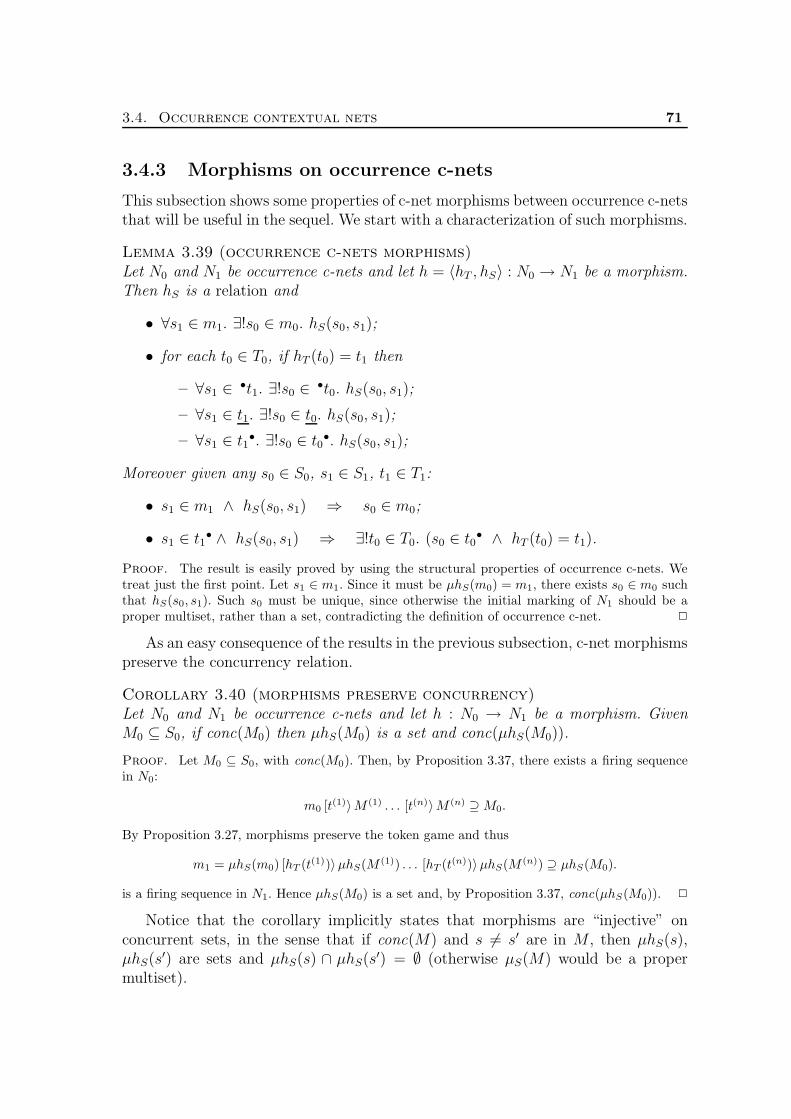
3.4. Occurrence contextual nets 71
3.4.3 Morphisms on occurrence c-nets
This subsection shows some properties of c-net morphisms between occurrence c-netsthat will be useful in the sequel. We start with a characterization of such morphisms.
Lemma 3.39 (occurrence c-nets morphisms)Let N0 and N1 be occurrence c-nets and let h = 〈hT , hS〉 : N0 → N1 be a morphism.Then hS is a relation and
• ∀s1 ∈ m1. ∃!s0 ∈ m0. hS(s0, s1);
• for each t0 ∈ T0, if hT (t0) = t1 then
– ∀s1 ∈•t1. ∃!s0 ∈
•t0. hS(s0, s1);
– ∀s1 ∈ t1. ∃!s0 ∈ t0. hS(s0, s1);
– ∀s1 ∈ t1•. ∃!s0 ∈ t0
•. hS(s0, s1);
Moreover given any s0 ∈ S0, s1 ∈ S1, t1 ∈ T1:
• s1 ∈ m1 ∧ hS(s0, s1) ⇒ s0 ∈ m0;
• s1 ∈ t1• ∧ hS(s0, s1) ⇒ ∃!t0 ∈ T0. (s0 ∈ t0
• ∧ hT (t0) = t1).
Proof. The result is easily proved by using the structural properties of occurrence c-nets. Wetreat just the first point. Let s1 ∈ m1. Since it must be µhS(m0) = m1, there exists s0 ∈ m0 suchthat hS(s0, s1). Such s0 must be unique, since otherwise the initial marking of N1 should be aproper multiset, rather than a set, contradicting the definition of occurrence c-net. 2
As an easy consequence of the results in the previous subsection, c-net morphismspreserve the concurrency relation.
Corollary 3.40 (morphisms preserve concurrency)Let N0 and N1 be occurrence c-nets and let h : N0 → N1 be a morphism. GivenM0 ⊆ S0, if conc(M0) then µhS(M0) is a set and conc(µhS(M0)).
Proof. Let M0 ⊆ S0, with conc(M0). Then, by Proposition 3.37, there exists a firing sequencein N0:
m0 [t(1)〉M (1) . . . [t(n)〉M (n) ⊇M0.
By Proposition 3.27, morphisms preserve the token game and thus
m1 = µhS(m0) [hT (t(1))〉µhS(M (1)) . . . [hT (t(n))〉µhS(M (n)) ⊇ µhS(M0).
is a firing sequence in N1. Hence µhS(M0) is a set and, by Proposition 3.37, conc(µhS(M0)). 2
Notice that the corollary implicitly states that morphisms are “injective” onconcurrent sets, in the sense that if conc(M) and s 6= s′ are in M , then µhS(s),µhS(s
′) are sets and µhS(s) ∩ µhS(s′) = ∅ (otherwise µS(M) would be a proper
multiset).

72 Chapter 3. Semantics of Contextual Nets
The next lemmata show that, more generally, morphisms preserve the “amountof concurrency”. Let the symbol ≺ denote the immediate causal dependency betweentransitions, namely t ≺ t′ if t < t′ and there does not exists t′′ such that t < t′′ < t′.First we prove that c-net morphisms reflect ≺-chains. Then, by means of some othertechnical results, we can conclude that c-net morphisms reflect causality and conflict,while asymmetric conflict is reflected or becomes conflict.
Lemma 3.41 (morphisms reflect ≺-chains)Let N0 and N1 be occurrence c-nets, let h : N0 → N1 be a morphism and let t
(0)1 ≺
t(1)1 ≺ . . . ≺ t
(n)1 be a chain of transitions in T1 such that t
(n)1 = hT (t
(n)0 ). Then
there exists a chain t(0)0 ≺ t
(1)0 ≺ . . . ≺ t
(n)0 in T0 such that t
(i)1 = hT (t
(i)0 ) for all
i ∈ 0, . . . , n.
Proof. We proceed by induction on n:
(n = 0) Obvious.
(n > 0) Let t(0)1 ≺ t
(1)1 ≺ . . . ≺ t
(n)1 = hT (t
(n)0 ). By inductive hypothesis (applied to the final part
of the chain) there is a chain t(1)0 ≺ . . . ≺ t
(n)0 such that t
(i)1 = hT (t
(i)0 ) for i ∈ 1, . . . , n.
Moreover, since t(0)1 ≺ t
(1)1 = hT (t
(1)0 ), two cases arise:
• t(0)1
• ∩ t(1)1 6= ∅.
Let s1 ∈ t(0)1
• ∩ t(1)1 . Since t
(1)1 = hT (t
(1)0 ) there is s0 ∈ t
(1)0 such that fS(s0, s1). Moreover,
by Lemma 3.39, from s1 ∈ t(0)1
• we have that that ∃!t(0)0 ∈ T0 such that hT (t
(0)0 ) = t
(0)1 and
s0 ∈ t(0)0
•. Therefore t(0)0 ≺ t
(1)0 is the transition that completes the chain.
• t(0)1
• ∩ •t(1)1 6= ∅.
Analogous to the previous case.2
Lemma 3.42Let N0 and N1 be occurrence c-nets and let h : N0 → N1 be a morphism. Then, forall t0, t
′0 ∈ T0, with hT (t0) 6= ⊥ 6= hT (t′0),
1. (hT (t0) = hT (t′0)) ∧ (t0 6= t′0) ⇒ t0#0t′0;
2. hT (t0) ≤1 hT (t′0) ⇒ ∃!t′′0 ∈ T0. (t′′0 ≤0 t′0 ∧ hT (t′′0) = hT (t0));
3. (a) hT (t0) 1 hT (t′0) ⇒ (t0 0 t′0) ∨ (t0#0t
′0);
(b) hT (t0) <1 hT (t′0) ⇒ (t0 <0 t′0) ∨ (t0#0t
′0);
Proof.
1. Let hT (t0) = hT (t′0) and t0 6= t′0. Consider a chain of transitions t(0)1 ≺ . . . ≺ t
(k)1 = hT (t0)
such that •t(0)1 ⊆ m1 and t
(i)1
• ∩ •t(i+1)1 6= ∅ for all i ∈ 0, . . . , k − 1 (the existence of
such a finite chain is an immediate consequence of the definition of occurrence c-net). ByLemma 3.41, we can find in T0 two ≺-chains of transitions,

3.4. Occurrence contextual nets 73
t(0)0 ≺ . . . ≺ t
(k)0 and t
′(0)0 ≺ . . . ≺ t
′(k)0 ,
such that, hT (t(i)0 ) = hT (t
′(i)0 ) = t
(i)1 , for all i ∈ 1, . . . , k and t0 = t
(k)0 , t′0 = t
′(k)0 .
Let j be the least index such that t(j)0 6= t
′(j)0 . If j = 0 (and thus •t
(j)1 ⊆ m1) consider a
generic s1 ∈•t
(0)1 . By definition of morphism, there are s0 ∈
•t(0)0 and s′0 ∈
•t′(0)0 such that
hS(s0, s1) and hS(s′0, s1). By Lemma 3.39, since s1 ∈ m1, also s0 and s′0 are in the initial
marking and thus s0 = s′0. Hence t(0)0 ր0 t
′(0)0 ր0 t
(0)0 , thus t
(0)0 #m
0 t′(0)0 and therefore, by
definition of #, t0#0t′0. If j > 0, then considering s1 ∈ t
(j−1)1
• ∩ •t(j)1 , the same reasoning
applies.
2. Existence easily follows from Lemma 3.41. As for uniqueness, let t′′′0 ≤0 t′0 and hT (t′′′0 ) =
hT (t0). If t′′′0 6= t′′0 then, by point (1) t′′′0 #0t′′0 and therefore t′0#0t
′0, contradicting the defini-
tion of occurrence c-net.
3. (a) Let hT (t0) 1 hT (t′0). Then there is a place s1 ∈ (hT (t0) ∪ •hT (t0)) ∩ •hT (t′0). Thus
there are s0 ∈ (t0 ∪•t0) such that hS(s0, s1) and s′0 ∈
•t′0 such that hS(s′0, s1). If s1 isin the initial marking then s0 = s′0 and thus t0 1 t
′0. Otherwise s0 and s′0 are in the
post-sets of two transitions t(0)0 and t
′(0)0 , which are mapped to the same transition in
N1 (the transition which has s1 in its post-set). By point (1), t(0)0 and t
′(0)0 are identical
or in conflict: in the first case s0 = s′0 and thus t0 0 t′0, while in the second case
t0#0t′0.
(b) Let hT (t0) <1 hT (t′0). By Lemma 3.41, there exists t′′0 ∈ T0 such that t′′0 <0 t′0 and
hT (t′′0 ) = hT (t0). It follows from point (1) that either t′′0 = t0 and thus t0 <0 t′0, or
t′′0#0t0 and thus t0#0t′0. 2
Corollary 3.43Let N0 and N1 be occurrence c-nets and let h : N0 → N1 be a morphism. Then, forall t0, t
′0 ∈ T0 with hT (t0) 6= ⊥ 6= hT (t′0),
1. ⌊hT (t0)⌋ ⊆ hT (⌊t0⌋);
2. (hT (t0) = hT (t′0)) ∧ (t0 6= t′0) ⇒ t0#0t′0;
3. hT (t0)ր1 hT (t′0) ⇒ (t0 ր0 t′0) ∨ (t0#0t
′0);
4. #hT (A) ⇒ #A′, for some A′ ⊆ A.
It is worth observing that, since the asymmetric conflict relation defined for anoccurrence c-net does not satisfy the saturation condition required for aes’s (seeDefinition 3.3) asymmetric conflict is not necessarily reflected by a c-net morphism,but it can also become conflict.

74 Chapter 3. Semantics of Contextual Nets
3.5 Unfolding: from semi-weighted to occurrence
contextual nets
This section shows how, given a semi-weighted c-net N , an unfolding constructionallows us to obtain an occurrence c-net Ua(N) that describes the behaviour of N .As for traditional nets, each transition in Ua(N) represents an instance of a precisefiring of a transition in N , and places in Ua(N) represent occurrences of tokensin the places of N . Each item (place or transition) of the unfolding is mapped tothe corresponding item of the original net by a c-net morphism fN : Ua(N) → N ,called the folding morphism. The unfolding operation can be extended to a functorUa : SW-CN→ O-CN that is right adjoint to the inclusion functor IO : O-CN→SW-CN and thus establishes a coreflection between SW-CN and O-CN.
We first introduce some technical notions. We say that a c-net N0 is a subnet ofN1, written N0 N1, if S0 ⊆ S1, T0 ⊆ T1 and the inclusion 〈iT , iS〉 (with iT (t) = t,for all t ∈ T0, and iS(s, s) = 1, for all s ∈ S0) is a c-net morphism. In words, N0 N1
if N0 coincides with an initial segment of N1. In the following it will be useful toconsider the subnets of an occurrence c-net obtained by truncating the original netat a given “causal depth”, where the notion of depth is defined in the natural way.
Definition 3.44 (depth)Let N be an occurrence c-net. The function depth : S∪T → N is defined inductivelyas follows:
depth(s) = 0 for s ∈ m;depth(t) = maxdepth(s) | s ∈ •t ∪ t+ 1 for t ∈ T ;depth(s) = depth(t) for s ∈ t•.
It is not difficult to prove that depth is a well-defined total function, since infinitedescending chains of causality are disallowed in occurrence c-nets. Moreover, givenan occurrence c-net N , the net containing only the items of depth less or equal tok, denoted by N [k], is a well-defined occurrence c-net and it is a subnet of N . Thefollowing simple result holds:
Proposition 3.45 (truncation)An occurrence c-net N is the (componentwise) union of its subnets N [k], of depth k.
The unfolding of a semi-weighted c-net N can be constructed inductively bystarting from the initial marking of N , and then by adding, at each step, an instanceof each transition of N enabled by (the image of) a concurrent subset of places inthe partial unfolding currently generated. For technical reasons we prefer to give anaxiomatic definition.

3.5. Unfolding: from semi-weighted to occurrence contextual nets 75
Definition 3.46 (unfolding)Let N be a semi-weighted c-net. The unfolding Ua(N) = 〈S ′, T ′, F ′, C ′, m′〉 of the netN and the folding morphism fN = 〈fT , fS〉 : Ua(N)→ N are the unique occurrencec-net and c-net morphism satisfying the following equations.
m′ = 〈∅, s〉 | s ∈ mS ′ = m′ ∪ 〈t′, s〉 | t′ = 〈Mp,Mc, t〉 ∈ T
′ ∧ s ∈ t•T ′ = 〈Mp,Mc, t〉 |Mp,Mc ⊆ S ′ ∧ Mp ∩Mc = ∅ ∧ conc(Mp ∪Mc) ∧
t ∈ T ∧ µfS(Mp) = •t ∧ [[t]] ≤ µfS(Mc) ≤ t
F ′pre(t′, s′) iff t′ = 〈Mp,Mc, t〉 ∧ s′ ∈ Mp (t ∈ T )
C ′(t′, s′) iff t′ = 〈Mp,Mc, t〉 ∧ s′ ∈ Mc (t ∈ T )F ′post(t
′, s′) iff s′ = 〈t′, s〉 (s ∈ S)
fT (t′) = t iff t′ = 〈Mp,Mc, t〉fS(s
′, s) iff s′ = 〈x, s〉 (x ∈ T ′ ∪ ∅)
The existence of the unfolding can be proved by explicitly giving its inductive defi-nition. Uniqueness follows from the fact that each item in a occurrence c-net has afinite depth.
Places and transitions in the unfolding of a c-net represent respectively tokensand firing of transitions in the original net. Each place in the unfolding is a pairrecording the “history” of the token and the corresponding place in the original net.Each transition is a triple recording the pre-set and context used in the firing, and thecorresponding transition in the original net. A new place with empty history 〈∅, s〉is generated for each place s in the initial marking of N . Moreover a new transitiont′ = 〈Mp,Mc, t〉 is inserted in the unfolding whenever we can find a concurrent setof places that corresponds, in the original net, to a marking that enables t (Mp ismapped to the pre-set and Mc to the context of t). For each place s in the post-setof such t, a new place 〈t′, s〉 is generated, belonging to the post-set of t′. The foldingmorphism f maps each place (transition) of the unfolding to the corresponding place(transition) in the original net. Figure 3.5 shows a c-net N and the initial part of its
unfolding (formally, it is the subnet of the unfolding of depth 3, namely Ua(N)[3]).The folding morphism is represented by labelling the items of the unfolding withthe names of the corresponding items of N .
Occurrence c-nets are particular semi-weighted c-nets, thus we can consider theinclusion functor IO : O-CN → SW-CN that acts as identity on objects andmorphisms. We show now that the unfolding of a c-net Ua(N) and the foldingmorphism fN are cofree over N . Therefore Ua extends to a functor that is rightadjoint to IO and thus establishes a coreflection between SW-CN and O-CN.

76 Chapter 3. Semantics of Contextual Nets
•s0
•s1
t0 •s2
t1s4
t2 t3
t4s3s5
N
•s0
•s1
t0 •s2
t1s4
t2 t3s1
t4s3 s3
t1s5
s1
t1s1
Ua(N)[3]
Figure 3.5: A c-net and (part of ) its unfolding.

3.5. Unfolding: from semi-weighted to occurrence contextual nets 77
Theorem 3.47 (coreflection between SW-CN and O-CN)IO ⊣ Ua
Proof. Let N be a semi-weighted c-net, let Ua(N) = 〈S′, T ′, F ′, C′,m′〉 be its unfolding andlet fN : Ua(N) → N be the folding morphism as in Definition 3.46. We have to show that forany occurrence c-net N1 and for any morphism g : N1 → N there exists a unique morphismh : N1 → Ua(N) such that the following diagram commutes:
Ua(N)fN
N
N1
hg
ExistenceWe define a sequence of morphisms h[k] : N1
[k] → Ua(N) such that, for any k,
h[k] ⊆ h[k+1] and fN h[k] = g|N1[k] ,
then the morphism h we are looking for will be h =⋃k h
[k]. We give an inductive definition:
(k = 0) The c-net N1[0] consists only of the initial marking of N1 with no transitions, i.e., N1
[0] =〈m1, ∅, ∅, ∅,m1〉. Therefore h[0] has to be defined:
hT[0] = ∅,
hS[0](s1, 〈∅, s〉) ≡ gS(s1, s) for all s1 ∈ S1
[0] = m1 and s ∈ S.
(k→ k + 1) The morphism h[k+1] extends h[k] on items with depth equal to k + 1 as follows. Lett1 ∈ T [k+1] with depth(t1) = k + 1. By definition of depth, depth(s) ≤ k for all s ∈ •t1 ∪ t1 and
thus h[k] is defined on the pre-set and on the context of t1. We must define hT on t1 and hS on itspost-set. Two cases arise:
• If gT (t1) = ⊥ then necessarily
hT[k+1](t1) = ⊥
hS[k+1](s1, s
′) = 0 for all s1 ∈ t1• and s′ ∈ S′.
• If gT (t1) = t then consider the sets
Mp = µhS[k]( •t1) Mc = µhS
[k](t1).
Since N1 is an occurrence c-net, •t1∩t1 = ∅ and, by Proposition 3.34, conc( •t1 ∪ t1). Hence,by Corollary 3.40,
Mp ∩Mc = ∅ and conc(Mp ∪Mc).
Moreover, by construction, fN h[k] = g|N1[k] , and therefore
µfS(Mp)
= µfS(µhS[k]( •t1))
= µgS( •t1)= •t [by def. of morphism]

78 Chapter 3. Semantics of Contextual Nets
and in the same way [[t]] ≤ µfS(Mc) ≤ t. Thus, by definition of unfolding, there exists atransition t′ = 〈Mp,Mc, t〉 in T ′.
It is clear that, to obtain a well defined morphism that makes the diagram commute, wehave to define
hT[k+1](t1) = t′
and, since µgS(t1•) = t•, for all s1 ∈ t1• and s ∈ t•
hS[k+1](s1, 〈t′, s〉) = gS(s1, s).
A routine checking allows to prove that, for each k, h[k] is a well-defined morphism andfN h[k] = g|N1
[k] .
UniquenessThe morphism h is clearly unique since at each step we were forced to define it as we did to ensurecommutativity. Formally, let h′ : N1 → Ua(N) be a morphism such that the diagram commutes,i.e., fN h′ = g. Then, we show, that for all k
h′|N1
[k] = h|N1[k] .
We proceed by induction on k:
(k = 0) The c-net N1[0] consists only of the initial marking of N1 and thus we have:
h′T[0]
= ∅ = hT[0],
h′S[0]
(s1, 〈∅, s〉) = gS(s1, s) = hS[0](s1, 〈∅, s〉), for all s1 ∈ S1
[0] = m1 and s ∈ S.
(k→ k + 1) For all t1 ∈ T [k+1], with depth(t1) = k + 1 we distinguish two cases:
• If gT (t1) = ⊥ then necessarily
h′T[k+1]
(t1) = ⊥ and µhS[k+1](t1
•) = ∅,
thus h′[k+1]
coincides with h[k+1], on t1 and its post-set.
• If gT (t1) = t then
h′T[k+1]
(t1) = t′ = 〈Mp,Mc, t〉 ∈ T ′,
with Mp = •t′ = µh′S( •t1) and Mc = t′ = µh′S(t1).5 By inductive hypothesis, since
depth(s1) ≤ k for all s1 ∈•t1 ∪ t1, we have that µhS( •t1) = Mp and µhS(t1) = Mc.
Therefore, by definition of h, hT (t1) = 〈Mp,Mc, t〉 = h′T (t1).
Moreover, for all s1 ∈ t1• and for all s ∈ t•, again by reasoning on commutativity of thediagram, h′S(s1, 〈t′, s〉) = gS(s1, s) = hS(s1, 〈t′, s〉).
2
5Notice that here equality holds since we are working with occurrence c-nets and thus contextscan only have multiplicity 1.

3.6. Occurrence contextual nets and asymmetric event structures 79
3.6 Occurrence contextual nets and asymmetric
event structures
This section shows that the semantics of semi-weighted c-nets given in terms of oc-currence c-nets can be abstracted to an event structure and to a domain semantics.First the existence of a coreflection between AES and O-CN is proved, substanti-ating the claim according to which aes’s represent a suitable model for giving eventbased semantics to c-nets. Then the coreflection between AES and Dom, definedin Section 3.1, can be exploited to complete the chain of coreflections from SW-CNto Dom.
Given an occurrence c-net we can obtain a pre-aes by simply forgetting theplaces, but remembering the dependency relations that they induce between transi-tions, namely causality and asymmetric conflict. The corresponding (saturated) aeshas the same causal relation ≤N , while asymmetric conflict is given by the unionof asymmetric conflict րN and of the induced binary conflict #N . Furthermore amorphism between occurrence c-nets naturally restricts to a morphism between thecorresponding aes’s.
Definition 3.48 (from occurrence c-nets to aes’s)Let Ea : O-CN→ AES be the functor defined as:
• for each occurrence c-net N , if #N denotes the induced binary conflict in N :
Ea(N) = 〈T,≤N ,րN ∪#N〉;
• for each morphism h : N0 → N1:
Ea(h : N0 → N1) = hT .
Notice that the induced conflict relation #a in the aes Ea(N) (see Definition 3.2)coincides with the induced conflict relation in the net N (see Definition 3.32). There-fore in the following we will confuse the two relations and simply write # to denoteboth of them.
Proposition 3.49 (well-definedness)Ea is a well-defined functor.
Proof. Given any occurrence c-net N , Definition 3.31 and the considerations on the saturationof pre-aes’s following Definition 3.3, immediately imply that Ea(N) is an aes. Furthermore, ifh : N0 → N1 is a c-net morphism, then, by Corollary 3.43, Ea(h) = hT is an aes-morphism.Finally Ea obviously preserves arrow composition and identities. 2
An aes can be identified with a canonical occurrence c-net, via a free constructionthat mimics Winskel’s: for each set of events related in a certain way by causality andasymmetric conflict we generate a unique place that induces such kind of relationson the events.

80 Chapter 3. Semantics of Contextual Nets
Definition 3.50 (from aes’s to occurrence c-nets)Let G = 〈E,≤,ր〉 be an aes. Then Na(G) is the net N = 〈S, T, F, C,m〉 definedas follows:
• m =
〈∅, A,B〉 |
A,B ⊆ E, ∀a ∈ A. ∀b ∈ B. aր b,∀b, b′ ∈ B. b 6= b′ ⇒ b#b′
;
• S = m ∪
〈e, A,B〉 |
A,B ⊆ E, e ∈ E, ∀x ∈ A ∪B. e < x,∀a ∈ A. ∀b ∈ B. aր b,∀b, b′ ∈ B. b 6= b′ ⇒ b#b′
;
• T = E;
• F = 〈Fpre, Fpost〉, with
Fpre = (e, s) | s = 〈x,A,B〉 ∈ S, e ∈ B,Fpost = (e, s) | s = 〈e, A,B〉 ∈ S;
• C = (e, s) | s = 〈x,A,B〉 ∈ S, e ∈ A.
The transitions of Na(G) are simply the events of G, while places are triples of theform 〈x,A,B〉, with x,A,B ⊆ E, and |x| ≤ 1. A place 〈x,A,B〉 is a preconditionfor all the events in B and a context for all the events in A. Moreover, if x = e,such a place is a postcondition for e, otherwise if x = ∅ the place belongs to theinitial marking. Therefore each place gives rise to a conflict between each pair of(distinct) events in B and to an asymmetric conflict between each pair of eventsa ∈ A and b ∈ B. Figure 3.6 presents some examples of basic aes’s with thecorresponding c-nets. The cases of an aes with two events related, respectively, bycausality, asymmetric conflict and (immediate symmetric) conflict are considered.Pictorially, an asymmetric conflict e0 ր e1 is represented by a dotted arrow from e0to e1. Causality is represented, as usual, by plain arrows.
The next proposition relates the causality and asymmetric conflict relations ofan aes with the corresponding relations of the c-net Na(G). In particular it is usefulin proving that Na(G) is indeed an occurrence c-net.
Lemma 3.51Let G = 〈E,≤,ր〉 be an aes and let Na(G) be the net N = 〈S, T, F, C,m〉. Thenfor all e, e′ ∈ E:
1. e <N e′ iff e < e′;
2. e N e′ iff eր e′;
3. eրN e′ iff eր e′.

3.6. Occurrence contextual nets and asymmetric event structures 81
G0
e0
e1
Na(G0)
•〈∅,∅,e0〉
•〈∅,e0,∅〉 e0 • 〈∅,e0,e1〉
〈e0,∅,∅〉
〈e0,∅,e1〉 • 〈∅,e0,e1,∅〉
•〈∅,∅,e1〉
•〈∅,e1,∅〉 e1 〈e0,e1,∅〉
〈e1,∅,∅〉
G1 e0 e1 Na(G1)
•
• e0 • •
• e1 •
G2 e0 e1 Na(G2)
• • • • •
• e0 • e1 •
Figure 3.6: Three simple aes’s and the corresponding occurrence c-nets producedby the functor Na.

82 Chapter 3. Semantics of Contextual Nets
Proof.
1. Let ≺N denote the immediate causality relation in N . If e ≺N e′ then there exists a place〈e, A,B〉 ∈ S with e′ ∈ A ∪B and thus, by definition of Na, e < e′. Vice versa, if e < e′
then 〈e, ∅, e′〉 ∈ S and thus e ≺N e′. Since <N is the transitive closure of ≺N and < isa transitive relation we conclude the thesis.
2. If e N e′ then there exists a place 〈x,A,B〉 ∈ S with e ∈ A∪B and e′ ∈ B and thus eithere ր e′ or e#e′. But since G is an aes, the binary conflict is included in the asymmetricconflict and thus, also in the second case, eր e′. Vice versa, if eր e′ then 〈∅, e, e′〉 ∈ Sand thus e N e′.
3. Immediate consequence of points (1) and (2).
2
As an immediate corollary we have:
Corollary 3.52Let G = 〈E,≤,ր〉 be an aes. Then Na(G) = N = 〈S, T, F, C,m〉 is an occurrencec-net.
Proof. By Lemma 3.51 the causality relation ≤N=≤ and the asymmetric conflictրN=ր inheritthe necessary properties from those of G. 2
Let G = 〈E,≤,ր〉 be an aes. For e ∈ E, we define the set of consequences⌈e⌉, as follows (considering the singleton e instead of e itself will simplify thenotation later).
⌈e⌉ = e′ ∈ E | e < e′.
This function is extended also to the empty set, by ⌈∅⌉ = E. We use the samenotation for occurrence c-nets, referring to the underlying aes.
The next technical lemma gives a property of morphisms between occurrencec-nets which will be useful in the proof of the coreflection result.
Lemma 3.53Let N0 and N1 be occurrence c-nets and let h : N0 → N1 be a morphism. For alls0 ∈ S0 and s1 ∈ S1, if hS(s0, s1) then
1. hT ( •s0) = •s1;
2. s0• = h−1
T (s1•) ∩ ⌈ •s0⌉;
3. s0 = h−1T (s1) ∩ ⌈
•s0⌉.

3.6. Occurrence contextual nets and asymmetric event structures 83
Proof. Let s0 ∈ S0 and s1 ∈ S1 such that hS(s0, s1).
1. If •s0 = ∅, i.e., s0 ∈ m0 then s1 ∈ m1 and thus •s1 = ∅ = hT ( •s0). Otherwise, let•s0 = t0.6 Therefore hT (t0) = t1 is defined (see the remark after Definition 3.26) ands1 ∈ t1•. Thus •s1 = t1 = hT ( •s0).
2. Let t0 ∈ s0•, i.e., s0 ∈ •t0. Since hS(s0, s1), we have that hT (t0) = t1 is defined and s1 ∈ •t1.Thus t0 ∈ h
−1T (s1
•) ∩ ⌈ •s0⌉.
For the converse inclusion, let t0 ∈ h−1T (s1
•) ∩ ⌈ •s0⌉. Then s1 ∈ •hT (t0) and thus there iss′0 ∈
•t0 such that hS(s′0, s1). Now, reasoning as in Lemma 3.42.(1), we conclude that s′0and s0 necessarily coincide, otherwise they would be in the post-condition of conflictingtransitions and thus, since t0 ∈ ⌈ •s0⌉, we would have t0#t0.
3. Analogous to (2). 2
Recall that, by Lemma 3.51, for any aes G = 〈E,≤,ր〉 the causality andasymmetric conflict relations in Na(G) coincide with ≤ andր. Hence Ea(Na(G)) =〈E,≤,ր′〉, where ր′=ր ∪# =ր, where the last equality is justified by the factthat in an aes # ⊆ր. Hence Ea Na is the identity on objects.
We next prove that Na extends to a functor from AES to O-CN, which is leftadjoint to Ea (with unit the identity idG). More precisely they establish a coreflectionfrom AES to O-CN.
Theorem 3.54 (coreflection between O-CN and AES)Na ⊣ Ea
Proof. Let G = 〈E,≤,ր〉 be an aes and let Na(G) = 〈S, T, F, C,m〉 be as in Definition 3.50.We have to show that for any occurrence c-net N0 and for any morphism g : G → Ea(N0) thereexists a unique morphism h : Na(G)→ N0, such that the following diagram commutes:
GidG
g
Ea(Na(G)) = G
Ea(h)
Ea(N0)
The behaviour of h on transitions is determined immediately by g:
hT = g.
Therefore we only have to show that a multirelation hS : S → S0 such that 〈hT , hS〉 is a morphismexists and is uniquely determined by hT .
ExistenceLet us define hS in such a way it satisfies the conditions of Lemma 3.53, specialized to the netNa(G), that is, for all s = 〈x,A,B〉 ∈ S and s0 ∈ S0:
6There is a unique transition generating s0, since N0 is an occurrence c-net.

84 Chapter 3. Semantics of Contextual Nets
hS(s, s0) iff ((x = ∅ ∧ s0 ∈ m0) ∨ (x = t ∧ s0 ∈ hT (t)•))∧ B = h−1
T (s0•) ∩ ⌈x⌉
∧ A = h−1T (s0) ∩ ⌈x⌉
To prove that the pair h = 〈hT , hS〉 is indeed a morphism, let us verify the conditions on thepreservation of the initial marking and of the pre-set, post-set and context of transitions.
First observe that µhS(m) = m0. In fact, if s = 〈x,A,B〉 ∈ m and hS(s, s0) then x = ∅ andthus, by definition of hS , s0 ∈ m0. Vice versa, let s0 ∈ m0 and let
A = h−1T (s0) and B = h−1
T (s0•)
Since t0#t′0 for all t0, t
′0 ∈ s0
• and t0 ր t′0 for all t0 ∈ s0, t′0 ∈ s0•, by definition of aes-morphism,
t#t′ for all t, t′ ∈ B and t ր t′ for all t ∈ A and t′ ∈ B. Hence there is a place s = 〈∅, A,B〉 ∈ mand hS(s, s0).
Now, let t ∈ T be any transition, such that hT (t) is defined. Then
• µhS( •t) = •hT (t).In fact, let s = 〈x,A,B〉 ∈ •t, that is t ∈ B, and let hS(s, s0). Then, by definition of hS ,hT (t) ∈ s0•, or equivalently s0 ∈ •hT (t). For the converse inclusion, let s0 ∈ •hT (t) andlet x = h−1
T ( •s0) ∩ ⌊t⌋. Since N0 is an occurrence c-net | •s0 |≤ 1 and thus | x |≤ 1 (moreprecisely x = ∅ if s0 ∈ m0, otherwise, x contains the unique t′ ≤ t, such that hT (t′) = t0,with •s0 = t0). Consider
A = h−1T (s0) ∩ ⌈x⌉ and B = h−1
T (s0•) ∩ ⌈x⌉.
Since t0#t′0 for all t0, t
′0 ∈ s0
• and t0 ր t′0 for all t0 ∈ s0, t′0 ∈ s0•, as in the previous case,
we have that s = 〈x,A,B〉 ∈ S is a place such that hS(s, s0). Clearly t ∈ ⌈x⌉, thus t ∈ Band therefore s ∈ •t and s0 ∈ µhS( •t).
• µhS(t) = hT (t).Analogous to the previous case.
• µhS(t•) = hT (t)•.If s = 〈x,A,B〉 ∈ t•, that is x = t, and hS(s, s0), then, by definition of hS , we haves0 ∈ hT (t)•. For the converse, let s0 ∈ hT (t)•. As above, consider
A = h−1T (s0) ∩ ⌈t⌉ and B = h−1
T (s0•) ∩ ⌈t⌉.
Then s = 〈t, A,B〉 ∈ t• and, by definition of hS, we have hS(s, s0).
Finally, if hT (t) is not defined, then the definition of hS implies that µhS(•t) = µhS(t) = µhS(t•) =∅. This concludes the proof that h is a morphism.
UniquenessThe multirelation hS such that 〈hT , hS〉 is a c-net morphism is unique essentially because it mustsatisfy the conditions of Lemma 3.53. More precisely, if h′S : S → S0 is another multirelation, suchthat 〈hT , h′S〉 is a morphism and h′S(s, s0) then necessarily by Lemma 3.53, hS(s, s0). Conversely,let hS(s, s0), with s = 〈x,A,B〉. Then, if x = ∅, by properties of net morphisms, s0 ∈ m0.Therefore there must be s′ ∈ m such that h′S(s′, s0). But, by Lemma 3.53 and definition of hS ,s′ = h−1
T (s0) = A and similarly s′• = h−1T (s0
•) = B. Therefore s′ = 〈∅, A,B〉 = s and thush′S(s, s0). An analogous reasoning allow us to conclude in the case x = t. 2
3.7. Processes of c-nets and their relation with the unfolding 85
We know by the previous theorem that Na extends to a functor from AES toO-CN. The behaviour of Na on morphisms is suggested by the proof of the theorem.Let h : G0 → G1, be an aes-morphism and let Na(Gi) = 〈Si, Ti, Fi, Ci, mi〉 fori ∈ 0, 1. Then Na(h) = 〈h, hS〉, with hS defined as follows:
• for all places 〈∅, A1, B1〉
hS(〈∅, h−1(A1), h
−1(B1)〉, 〈∅, A1, B1〉)
• for all e0 ∈ T0 such that hT (e0) = e1 and for all places 〈e1, A1, B1〉
hS(〈e0, h−1(A1) ∩ ⌈e0⌉, h
−1(B1) ∩ ⌈e0⌉〉, 〈e1, A1, B1〉)
Finally, notice that the equivalence between PES and Dom (see Section 2.4)can be used to “translate” the domain semantics of semi-weighted c-nets into aprime event structure semantics. This completes the following chain of coreflectionsbetween SW-CN and PES
SW-CNUa
⊥ O-CNEa
⊥
IO
AESLa
⊥
Na
DomPa
P
∼ PESL
Figure 3.7 shows (part of) the aes, the domain and the pes associated to the c-netof Figure 3.5. Although (for the sake of readability) not explicitly drawn, in the pesall the “copies” of t4, namely the events tx4 are in conflict.
We remark that the pes semantics is obtained from the aes semantics by intro-ducing an event for each possible different history of events in the aes. For instance,the pes semantics of the net N0 in Figure 3.8 is given by P , where e′1 represents thefiring of the transition t1 by itself, with an empty history, and e′′1 the firing of thetransition t1 after t0. Obviously the aes semantics is finer than the pes semantics,or in other words the translation from AES to PES causes a loss of information.For example, the nets N3 and N ′3 in Figure 3.8 have the same pes semantics, butdifferent aes semantics.
3.7 Processes of c-nets and their relation with the
unfolding
The notion of occurrence c-net introduced in Section 3.4 naturally suggests a no-tion of nondeterministic process for c-nets, which can be defined as an occur-rence c-net with a morphism (mapping places into places and total on transi-tions) to the original net. Deterministic c-net processes can then be defined asparticular nondeterministic processes such that the underlying occurrence c-netsatisfies a further conflict-freeness requirement. Interestingly, the resulting notion

86 Chapter 3. Semantics of Contextual Nets
t0
t′1 t4 t2 t3
t′′1
t′′′1
t0
t′1 # t4 t2# t3#
t′4 t′′1 ## t′24 t24
t′′4 t′′′1# # t′′24
(a) Ea(Ua(N)) (c) P(La(Ea(Ua(N))))
∅
t0 t3
t0, t′1 t0, t4 t0, t2 t0, t3
t0, t′1, t4 t0, t′1, t′′1 t0, t′1, t2 t0, t′1, t3 t0, t2, t4 t0, t3, t4
t0, t′1, t
′′1 , t4 t0, t
′1, t
′′1 , t
′′′1 t0, t
′1, t3, t4 t0, t
′1, t
′′1 , t2 t0, t
′1, t
′′1 , t3 t0, t
′1, t2, t4
. . . . . . . . . . . .
(b) La(Ea(Ua(N)))
Figure 3.7: The (a) aes (b) domain and (c) pes for the c-net N of Figure 3.5

3.7. Processes of c-nets and their relation with the unfolding 87
•
t0 •
t1
e1 e2
•
t1 t0
t′1
e′1#
e0
e′′1
N3 G = Ea(N3) N ′3P = Ea(N
′3)
= P(La(Ea(N3)))
Figure 3.8: aes semantics is finer than pes semantics.
of deterministic process turns out to coincide with those proposed by other au-thors [Vog97b, Ris94, GM98, Win98, Bus98] (see Section 2.3). It is worth recallingthat the stress on the necessity of using an additional relation of “weak-causality”to be able to fully express the causal structure of net computations in the presenceof read or inhibitor arcs can be found already in [JK93, JK95]. However, we alreadyobserved that a different notion of enabling allowing for the simultaneous firing ofweakly dependent transitions is used in [JK95], making difficult a complete directcomparison. For the same reason, although “syntactically” the processes of [Vog97b]coincide with ours, they are intended to represent the same firing sequences, but dif-ferent step sequences.
The papers [GM98, Win98] extend the theory of concatenable processes of or-dinary nets [DMM89] to c-nets, by showing that the concatenable processes of ac-net N form the arrows of a symmetric monoidal category CP[N ], where objectsare the elements of the free commutative monoid over the set of places (multisets ofplaces). In particular, in [GM98] a purely algebraic characterization of such categoryis given.
Since the category CP[N ] of concatenable processes of a net N provides a com-putational model for N , describing its operational behaviour, we are naturally leadto compare such semantics with the one based on the unfolding. This section, relyingon the notion of concatenable c-net process and exploiting the chain of coreflectionsleading from SW-CN to Dom, establishes a close relationship between process andunfolding semantics for c-nets. More precisely, we generalize to c-nets (in the semi-weighted case) a result proved in [MMS96] for ordinary nets, stating that the domainLa(Ea(Ua(N))) associated to a semi-weighted net N coincides with the completionof the preorder obtained as the comma category of CP[N ] under the initial marking.Roughly speaking, the result says that the domain obtained via the unfolding of ac-net can be equivalently described as the collection of the deterministic processesof the net, ordered by prefix.

88 Chapter 3. Semantics of Contextual Nets
3.7.1 Contextual nets processes
A process of a c-net N can be naturally defined as an occurrence c-net Nϕ, togetherwith a morphism ϕ to the original net. In fact, since morphisms preserve the tokengame, ϕ maps computations of Nϕ into computations of N in such a way that theprocess can be seen as a representative of a set of possible computations of N . Theoccurrence c-net Nϕ makes explicit the causal structure of such computations sinceeach transition is fired at most once and each place is filled at most with one tokenduring each computation. In this way (as it happens in the unfolding) transitionsand places of Nϕ can be thought of, respectively, as instances of firing of transitionsand tokens in places of the original net. Actually, to allow for such an interpretation,some further restrictions have to be imposed on the morphism ϕ, namely it mustmap places into places (rather than into multisets of places) and it must be total ontransitions.
Besides “marked processes”, representing computations of the net starting fromthe initial marking, we will introduce also “unmarked processes”, representing com-putations starting from a generic marking. This is needed to be able to define ameaningful notion of concatenation between processes.
Definition 3.55 ((nondeterministic) process)A marked process of a c-net N = 〈S, T, F, C,m〉 is a mapping ϕ : Nϕ → N ,where Nϕ is an occurrence c-net and ϕ is a strong c-net morphism, namely a c-netmorphism such that ϕT is total and ϕS maps places into places. The process is calleddiscrete if Nϕ has no transitions.
An unmarked process of N is defined in the same way, where the mapping ϕ isan “unmarked morphism”, namely ϕ is not required to preserve the initial marking(it satisfies all conditions of Definition 3.26, but (1)).
Equivalently, if we denote by CN∗ the subcategory of CN where the arrows arestrong c-net morphisms, the processes of N can be seen as objects of the commacategory 〈O-CN ↓ N〉 in CN∗. This gives also the (obvious) notion of isomorphismbetween processes, which is an isomorphism between the underlying occurrence nets“consistent” with the mappings to the original net. Analogous definitions can begiven also for the unmarked processes of a net N .7
A deterministic process represents a set of computations which differ only forthe order in which independent transitions are fired. In our setting a deterministicprocess is thus defined as a process such that, in the underlying occurrence net, thetransitive closure of asymmetric conflict is a finitary partial order, in such a way
7It is worth remarking that if we want each truly concurrent computation of the net N to berepresented by at most one configuration of the nondeterministic process, an additional constraintmust be imposed on ϕ, requiring that •t1 = •t2, t1 = t2 and ϕ(t1) = ϕ(t2) implies t1 = t2, as in[VSY98]. However, the two notions of process collapse when we restrict to deterministic processeswhich are the focus of this section.

3.7. Processes of c-nets and their relation with the unfolding 89
that all transitions can be fired in a single computation of the net. Deterministicoccurrence c-nets will be always denoted by O, possibly with subscripts.
Definition 3.56 (deterministic occurrence c-net)An occurrence c-net O is called deterministic if the asymmetric conflictրO is acyclicand well-founded.
Equivalently, one could have asked the transitive closure of the asymmetric conflictrelation (րO)∗ to be a partial order, such that for each transition t in O, the sett′ | t′(րO)∗t is finite. Alternatively, it can be easily seen that a finite occurrencec-net is deterministic if and only if the corresponding aes is conflict free.
We denote by min(O) and max(O) the sets of minimal and maximal places of Owith respect to the partial order ≤O.
Definition 3.57 (deterministic process)A (marked or unmarked) process ϕ is called deterministic if the occurrence c-net Oϕ
is deterministic. The process is finite if the set of transitions in Oϕ is finite. In thiscase, we denote by min(ϕ) and max(ϕ) the sets min(Oϕ) and max(Oϕ), respectively.Moreover we denote with •ϕ and ϕ• the multisets µϕS(min(ϕ)) and µϕS(max(ϕ)),called respectively the source and the target of ϕ.
Clearly, in the case of a marked process ϕ of a c-net N , the marking •ϕ coincideswith the initial marking of N .
3.7.2 Concatenable processes
As in [GM98, Win98] a notion of concatenable process for contextual nets, endowedwith an operation of sequential (and parallel) composition, can be easily defined,generalizing the concatenable processes of [DMM89]. Obviously a meaningful op-eration of sequential composition can be defined only on the unmarked processesof a c-net. In order to properly define the operation of concatenation of processes,we need to impose a suitable ordering over the places in min(ϕ) and max(ϕ) foreach process ϕ. Such ordering allows one to distinguish among “interface” places ofOϕ which are mapped to the same place of the original net, a capability which isessential to make sequential composition consistent with the causal dependencies.
Definition 3.58Let A and B be sets and let f : A → B be a function. An f -indexed ordering is afamily α = αb | b ∈ B of bijections αb : f−1(b) → [|f−1(b)|], where [i] denotes thesubset 1, . . . , i of N, and f−1(b) = a ∈ A | f(a) = b.
The f -indexed ordering α will be often identified with the function from A to N itnaturally induces (formally defined as
⋃b∈B αb).
90 Chapter 3. Semantics of Contextual Nets
Definition 3.59 (concatenable process)A concatenable process of a c-net N is a triple γ = 〈µ, ϕ, ν〉, where
• ϕ is a finite deterministic unmarked process of N ;
• µ is ϕ-indexed ordering of min(ϕ);
• ν is ϕ-indexed ordering of max(ϕ).
Two concatenable processes γ1 = 〈µ1, ϕ1, ν1〉 and γ2 = 〈µ2, ϕ2, ν2〉 of a c-net Nare isomorphic if there exists an isomorphism of processes f : ϕ1 → ϕ2, consistentwith the decorations, i.e., such that µ2(fS(s1)) = µ1(s1) for each s1 ∈ min(ϕ1) andν2(fS(s1)) = ν1(s1) for each s1 ∈ max(ϕ1). An isomorphism class of processes iscalled (abstract) concatenable process and denoted by [γ], where γ is a member ofthat class. In the following we will often omit the word “abstract” and write γ todenote the corresponding equivalence class.
The operation of sequential composition on concatenable processes is defined inthe natural way. Given two concatenable processes 〈µ1, ϕ1, ν1〉 and 〈µ2, ϕ2, ν2〉, suchthat ϕ1
• = •ϕ2 their concatenation is defined as the process obtained by gluing themaximal places of ϕ1 and the minimal places of ϕ2 according to the ordering of suchplaces.
Definition 3.60 (sequential composition)Let γ1 = 〈µ1, ϕ1, ν1〉 and γ2 = 〈µ2, ϕ2, ν2〉 be two concatenable processes of a c-netN such that ϕ1
• = •ϕ2. Suppose T1 ∩ T2 = ∅ and S1 ∩ S2 = max(ϕ1) = min(ϕ2),with ϕ1(s) = ϕ2(s) and ν1(s) = µ2(s) for each s ∈ S1 ∩ S2. In words γ1 and γ2
overlap only on max(ϕ1) = min(ϕ2), and on such places the labelling on the originalnet and the ordering coincide. Then their concatenation γ1; γ2 is the concatenableprocess γ = 〈µ1, ϕ, ν2〉, where the process ϕ is the (componentwise) union of ϕ1 andϕ2
It is easy to see that concatenation induces a well-defined operation of sequentialcomposition between abstract processes. In particular, if [γ1] and [γ2] are abstractconcatenable processes such that γ1
• = •γ2 then we can always find γ′2 ∈ [γ2]such that γ1; γ
′2 is defined. Moreover the result of the composition at abstract level,
namely [γ1; γ′2], does not depend on the particular choice of the representatives.
Definition 3.61 (category of concatenable processes)Let N be a c-net. The category of (abstract) concatenable processes of N , denoted byCP[N ], is defined as follows. Objects are multisets of places of N , namely elementsof µS. Each (abstract) concatenable process [〈µ, ϕ, ν〉] of N is an arrow from •ϕ toϕ•.
One could also define a tensor operation ⊗, modelling parallel composition of pro-cesses, making the category CP[N ] a symmetric monoidal category (the symmetriesbeing the discrete processes). Since such operation is not relevant for our presentaim, we refer the interested reader to [GM98, Win98].

3.7. Processes of c-nets and their relation with the unfolding 91
3.7.3 Relating processes and unfolding
Let N = 〈S, T, F, C,m〉 be a c-net and consider the comma category 〈m ↓ CP[N ]〉.The objects of such category are concatenable processes ofN starting from the initialmarking. An arrow exists from a process γ1 to γ2 if the second one can be obtainedby concatenating the first one with a third process γ. This can be interpreted as akind of prefix ordering.
Lemma 3.62Let N = 〈S, T, F, C,m〉 be a c-net. Then the comma category 〈m ↓ CP[N ]〉 is apreorder.
Proof. Let γi : m→Mi (i ∈ 1, 2) be two objects in 〈m ↓ CP[N ]〉, and suppose there are twoarrows γ′, γ′′ : γ1 → γ2. By definition of comma category γ1; γ
′ = γ1; γ′′ = γ2, which, by definition
of sequential composition, easily implies γ′ = γ′′. 2
In the sequel the preorder relation over 〈m ↓ CP[N ]〉 (induced by sequentialcomposition) will be denoted by .N or simply by ., when the net N is clear fromthe context. Therefore γ1 . γ2 if there exists γ such that γ1; γ = γ2.
We provide an alternative characterization of the preorder relation .N which willbe useful in the sequel. It essentially formalizes the intuition given above, accordingto which the preorder on 〈m ↓ CP[N ]〉 is a generalization of the prefix relation.First, we need to introduce the notion of left-injection for processes.
Definition 3.63 (left injection)Let γi : m→Mi (i ∈ 1, 2) be two objects in 〈m ↓ CP[N ]〉, with γi = 〈µi, ϕi, νi〉. Aleft injection ι : γ1 → γ2 is a morphism of marked processes ι : ϕ1 → ϕ2, such that
1. ι is consistent with the indexing of minimal places, namely µ1(s) = µ2(ι(s))for all s ∈ min(ϕ1);
2. ι is “rigid” on transitions, namely for t′2 in Oϕ2 and t1 in Oϕ1, if t′2 ր ι(t1)then t′2 = ι(t′1) for some t′1 in Oϕ1.
The name “injection” is justified by the fact that a morphism ι between markeddeterministic processes (being a morphism between the underlying deterministicoccurrence c-nets) is injective on places and transitions, as it can be shown easilyby using the properties of (occurrence) c-nets morphisms proved in Section 3.4. Theword “left” is instead related to the requirement of consistency with the decorationof the minimal items. Finally, the rigidity of the morphism ensures that γ2 does notextend γ1 with transitions inhibited in γ1.
Lemma 3.64Let γi : m → Mi (i ∈ 1, 2) be two objects in 〈m ↓ CP[N ]〉, with γi = 〈µi, ϕi, νi〉.Then
γ1 . γ2 iff there exists a left injection ι : γ1 → γ2.
92 Chapter 3. Semantics of Contextual Nets
Proof. (⇒) Let γ1 . γ2, namely γ2 = γ1; γ for some process γ = 〈µ, ϕ, ν〉. Without loss ofgenerality, we can assume that ϕ2 is obtained as the componentwise union of ϕ1 and ϕ and thisimmediately gives a morphism of marked processes (the inclusion) ι : ϕ1 → ϕ2, consistent withthe indexing of minimal places. To conclude it remains only to show that ι is rigid. Suppose thatt′2 ր ι(t1) for some transitions t1 in Oϕ1 and t′2 in Oϕ2 , and thus, by Definition 3.30, eithert′2 ι(t1) or t′2 < ι(t1). To conclude that ι is rigid we must show that in both cases t′2 is in Oϕ1 .
• If t′2 ι(t1), since the process ϕ2 is deterministic, t′2 and ι(t1) cannot be in conflict andthus it must be t′2 ∩
•ι(t1) 6= ∅. Since t′2 uses as context a place which is not maximal inOϕ1 , necessarily t′2 is in Oϕ1 , otherwise it could not be added by concatenating ϕ to ϕ1.
• If t′2 < ι(t1) then we can find a transition t′3 in Oϕ2 such that t′2 < t′3 and t′3•∩(•ι(t1)∪ι(t1)).
As above, t′3 must be in Oϕ1 since it uses as postcondition a place in Oϕ1 . An inductivereasoning based on this argument shows that also t′2 is in Oϕ1 .
(⇐) Let ι : γ1 → γ2 be a left injection. We can suppose without loss of generality thatOϕ1 is a subnet of Oϕ2 , in such a way that ι is the inclusion and µ1 = µ2. Let Oϕ be the net(Oϕ2 − Oϕ1) ∪max(Oϕ1), where difference and union are defined componentwise. More preciselyOϕ = 〈S, T, F, C〉, with:
• S = (S2 − S1) ∪max(ϕ1)
• T = T2 − T1
• the relations F and C are the restrictions of F2 and C2 to T .
It is easy to see that Oϕ is a well-defined occurrence c-net and min(Oϕ) = max(Oϕ1). In particular,the fact that F is well-defined namely that if t ∈ T then •t, t• ⊆ S immediately derives from the factthat the inclusion ι is a morphism of deterministic occurrence c-nets. Instead the well-definednessof C is related to the fact that the injection is rigid. In fact, let s ∈ t for t ∈ T and suppose thats 6∈ S. Therefore s ∈ •t1, for some t1 ∈ T1 and thus t ր t1, which, by rigidity, implies t ∈ T1,contradicting t ∈ T .
Therefore if we denote by γ the concatenable process 〈ν1, ϕ, ν2〉, then γ1; γ = γ2, and thusγ1 . γ2. 2
We can show now that the ideal completion of the preorder 〈m ↓ CP[N ]〉is isomorphic to the domain obtained from the unfolding of the net N , namelyLa(Ea(Ua(N))). Besides exploiting the characterization of the preorder relation on〈m ↓ CP[N ]〉 given above, the result strongly relies on the description of the un-folding construction as chain of adjunctions.
First, it is worth recalling some definitions and results on the ideal completionof (pre)orders.
Definition 3.65 (ideal)Let P be a preorder. An ideal of P is a subset S ⊆ P , directed and downward closed(namely S =
⋃↓ x | x ∈ S). The set of ideals of P , ordered by subset inclusion is
denoted by Idl(P ).
Given a preorder P , the partial order Idl(P ) is an algebraic cpo, with compactelements K(Idl(P )) = ↓ p | p ∈ P. Moreover Idl(P ) ≃ Idl(P/≡), where P/≡ is thepartial order induced by the preorder P . Finally, recall that if D is an algebraic cpo,then Idl(K(D)) ≃ D.

3.7. Processes of c-nets and their relation with the unfolding 93
Lemma 3.66Let P1 and P2 be preorders and let f : P1 → P2 be a surjective function such thatp1 ⊑ p′1 iff f(p1) ⊑ f(p′1). Then the function f ∗ : Idl(P1) → Idl(P2), defined byf ∗(I) = f(x) | x ∈ I, for I ∈ Idl(P1), is an isomorphism of partial orders.
Proof. The function f∗ is surjective since for every ideal I2 ∈ Idl(P2) it can be easily proved thatf−1(I2) is an ideal and f∗(f−1(I2)) = I2 by surjectivity of f . Moreover, notice that if I1, I
′1 ∈ Idl(P1)
are two ideals then I1 ⊆ I ′1 if and only if f∗(I1) ⊆ f∗(I ′1). The right implication is obvious. For theleft one, assume f∗(I1) ⊆ f∗(I ′1). Then observe that if x ∈ I1 then f(x) ∈ f∗(I1) ⊆ f∗(I ′1). Hencethere exists x′ ∈ I ′1 such that f(x′) = f(x). Thus by hypothesis on f we have x ⊑ x′ and therefore,by definition of ideal, x ∈ I ′1.
Then we can conclude that f∗ is also injective, thus it is a bijection, and clearly f∗ as well asits inverse are monotone functions. 2
Notice that in particular, if P is a preorder, D is an algebraic cpo and f : P →K(D) is a surjection such that p ⊑ p′ iff f(p) ⊑ f(p′), then Idl(P ) ≃ Idl(K(D)) ≃ D.
We can now prove the main result of this section, which establishes a tightrelationship between the unfolding and the process semantics of semi-weighted c-nets. We show that the ideal completion of the preorder 〈m ↓ CP[N ]〉 and thedomain associated to the net N through the unfolding construction are isomorphic.To understand which is the meaning of taking the ideal completion of the preorder〈m ↓ CP[N ]〉, first notice that the elements of the partial order induced by thepreorder 〈m ↓ CP[N ]〉 are classes of concatenable processes with respect to anequivalence ≡l defined by γ1 ≡l γ2 if there exist a discrete concatenable processγ such that γ1; γ = γ2. In other words, γ1 ≡l γ2 can be read as “γ1 and γ2 leftisomorphic”, where “left” means that the isomorphism is required to be consistentonly with respect to the ordering of the minimal places. Since the net N is semi-weighted, the equivalence ≡l turns out to coincide with the isomorphism of markedprocesses. In fact, being the initial marking of N a set, only one possible orderingfunction exists for the minimal places of a marked process. Finally, since processesare finite, taking the ideal completion of the partial order induced by the preorder〈m ↓ CP[N ]〉 (which produces the same result as taking directly the ideal completionof 〈m ↓ CP[N ]〉) is necessary to move from finite computations to arbitrary ones.
Theorem 3.67 (unfolding vs. concatenable processes)Let N be a semi-weighted c-net. Then the ideal completion of 〈m ↓ CP[N ]〉 isisomorphic to the domain La(Ea(Ua(N))).
Proof. Let N = 〈S, T, F, C,m〉 be a c-net. It is worth recalling that the compact elements of thedomain La(Ea(Ua(N))), associated to N , are exactly the finite configurations of Ea(Ua(N)), asshown in Theorem 3.19. By Lemma 3.66, to prove the thesis it suffices to show that it is possibleto define a function ξ : 〈m ↓ CP[N ]〉 → K(La(Ea(Ua(N)))) such that f is surjective, and for allγ1, γ2 in 〈m ↓ CP[N ]〉,
γ1 . γ2 iff ξ(γ1) ⊑ ξ(γ2).
The function ξ can be defined as follows. Let γ = 〈µ, ϕ, ν〉 be a concatenable process in〈m ↓ CP[N ]〉. Being ϕ a marked process of N (and thus a c-net morphism ϕ : Oϕ → N), by

94 Chapter 3. Semantics of Contextual Nets
the universal property of coreflections, there exists a unique arrow ϕ′ : Oϕ → Ua(N), making thediagram below commute.
Ua(N)fN
N
Oϕ
ϕ′
ϕ
In other words, the coreflection between SW-CN and O-CN gives a one-to-one correspondencebetween the (marked) processes of N and of those of its unfolding Ua(N).
Then we define ξ(γ) = ϕ′T (Tϕ), where Tϕ is the set of transitions of Oϕ. To see that ξ is a well
defined function, just observe that it could have been written, more precisely, as Ea(Ua(ϕ))(Tϕ)and Tϕ is a configuration of Ea(Ua(Oϕ)) = Ea(Oϕ) since Oϕ is a deterministic occurrence c-net.
• ξ is surjectiveLet C ∈ K(La(Ea(Ua(N)))) be a finite configuration. Then C determines a deterministicprocess ϕ′
C : Oϕ′
C→ Ua(N) of the unfolding of N , having C as set of transitions.8 Thus
ϕ = fN ϕ′C is a deterministic process of N , and, by the definition of ξ, we immediately
get that ξ(ϕ) = ϕ′C(Tϕ′
C) = C.
• ξ is monotoneLet γ1 and γ2 be processes in 〈m ↓ CP[N ]〉 and let γ1 . γ2. Then, by Lemma 3.64 thereexists a left-injection ι : γ1 → γ2. The picture below illustrates the situation, by depictingalso the processes ϕ′
1 and ϕ′2 of the unfolding of N , induced by ϕ1 and ϕ2, respectively.
Ua(N)fN
N
Oϕ2
ϕ′
2
ϕ2
Oϕ1
ι
ϕ′
1 ϕ1
We have that ξ(γ1) = ϕ′1(Tϕ1) = ϕ′
2(ι(Tϕ1)) ⊆ ϕ′2(Tϕ2) = ξ(γ2). Therefore, to conclude that
ξ(γ1) ⊑ ξ(γ2) we must show that also the second condition of Definition 3.13 is satisfied.Let t2 ∈ ξ(γ2) and t1 ∈ ξ(γ1), with t2 ր t1. By definition of ξ, ti = ϕi(t
′i) with t′i in Oϕi
,for i ∈ 1, 2 and thus:
ϕ′2(t
′2)ր ϕ′
1(t′1) = ϕ′
2(ι(t′1))
By properties of occurrence net morphisms (Corollary 3.43 and the fact that Oϕ2 isdeterministic), this implies t′2 ր ι(t′1) and thus, being ι a left injection, by rigidity t′2 = ι(t)for some t in Oϕ1 . Therefore t2 = ϕ′
2(t′2) = ϕ′
2(ι(t)) = ϕ′1(t) belongs to ξ(γ1), as desired.
8Essentially Oϕ′
Cis the obvious subnet of Ua(N) having C as set of transitions and ϕ′
C is aninclusion.

3.7. Processes of c-nets and their relation with the unfolding 95
• ξ(γ1) ⊑ ξ(γ2) implies γ1 . γ2.Let ξ(γ1) ⊑ ξ(γ2). The inclusion ξ(γ1) ⊆ ξ(γ2), immediately induces a mapping ι of thetransitions of Oϕ1 into the transitions of Oϕ2 , defined by ι(t1) = t2 if ϕ′
1(t1) = ϕ′2(t2) (see
the picture above). This function is well-defined since processes are deterministic and thusmorphisms ϕ′
i are injective. Since the initial marking of N is a set, the mapping of min(ϕ1)into min(ϕ2) is uniquely determined and thus ι uniquely extends to places becoming a(marked) process morphism between ϕ1 and ϕ2. Again for the fact that N is semi-weighted(and thus there exists a unique indexing for the minimal places of each process startingfrom the initial marking) such morphism is consistent with the indexing of minimal places.Finally, ι is rigid. In fact, let t2 ր ι(t1), for t1 in Oϕ1 and t2 in Oϕ2 . By definition of c-netmorphism (Definition 3.26), recalling that ϕ2 is total both on places and transitions, wededuce ϕ′
2(t2)ր ϕ′2(ι(t1)). The way ι is defined implies that ϕ′
2(ι(t1)) = ϕ′1(t1), and thus
ϕ′2(t2)ր ϕ′
1(t1).
Since ϕ′i(ti) ∈ ξ(γi) for i ∈ 1, 2, by definition of the order on configurations, we immedi-
ately have that ϕ′2(t2) ∈ ξ(γ1), thus there is t′1 in Oϕ1 such that ϕ′
1(t′1) = ϕ′
2(t2), and thusι(t′1) = t2.
By lemma 3.64, the existence of the left injection ι : γ1 → γ2, implies γ1 . γ2.2


Chapter 4
Semantics of Inhibitor Nets
The work developed in the previous chapter for contextual nets is extended here tonets with contextual and inhibitor arcs, called inhibitor nets, where transitions cancheck both for the presence and the absence of tokens in the places of the net. To dealwith the non-monotonic features introduced by the presence of inhibitor arcs, we de-fine inhibitor event structures (or ies for short), a new event structure model whichproperly generalizes aes’s. In such structures a relation, called disabling-enablingrelation, allows one to model, in a compact way, the presence of disjunctive conflict-ing causes and the situations of relative atomicity of pairs of events, determined byinhibitor arcs. The same relation permits to represent, as particular cases, also therelations of causality and asymmetric conflict already present in asymmetric eventstructures.
Following the general methodology outlined in the Introduction, the trulyconcurrent semantics for inhibitor nets is given via a chain of functors leading fromthe category SW-IN of semi-weighted inhibitor nets to the category Dom of finitaryprime algebraic domains:
SW-INUi
⊥ O-INEi
IO
IESLi
⊥ Dom
Pi
P
∼ PESL
The unfolding and its characterization as a universal construction are “lifted” fromcontextual to inhibitor nets. Roughly speaking, to construct the unfolding of aninhibitor net N we unfold the contextual net obtained from N by forgetting theinhibitor arcs and then we enrich the resulting occurrence contextual net by addingagain the original inhibitor arcs. In this way the unfolding remains decidable, theprice to pay being the presence of non-executable events in the resulting occurrenceinhibitor net. The unfolding can be naturally abstracted to an ies and then to aprime algebraic domain. The main difference with respect to contextual nets is theabsence of a functor performing the backward step from ies’s to occurrence inhibitornets. We argue that, under reasonable assumptions on the notions of occurrence netand of unfolding, the problem has no solutions, being basically related to the thecomplex kind of causality expressible in ies’s.

98 Chapter 4. Semantics of Inhibitor Nets
Finally, the above semantics is shown to fit nicely with some of the deterministicprocess semantics proposed in the literature for inhibitor nets. We compare the twoapproaches by characterizing the domain associated to the unfolding of a net as thepartial order of processes starting from its initial marking. To this aim a small gapexisting between the process semantics of ordinary and inhibitor nets has to be filledwith the introduction of an appropriate notion of concatenable process for inhibitornets.
The rest of the chapter is organized as follows. Section 4.1 motivates and de-fines inhibitor event structures, by showing that they properly generalize asymmet-ric event structures. Section 4.2 studies the relation between ies’s and domains,which is formalized as a categorical coreflection between IES and Dom. Section 4.3presents the category of inhibitor nets and focuses on the subcategory SW-IN of(semi-weighted) inhibitor nets which we shall work with. Section 4.4 introduces thecategory of occurrence inhibitor nets and generalizes the unfolding construction fromcontextual to inhibitor nets. Section 4.5 shows how the unfolding can be abstractedto an ies semantics. Finally Section 4.6 discusses the relation between the unfoldingand the deterministic process semantics of inhibitor nets.
4.1 Inhibitor event structures
In the previous chapter, to model in a direct way the behaviour of contextual nets,we generalized prime event structures by replacing the symmetric conflict with anasymmetric conflict relation. Such a feature is obviously still necessary to be ableto model the dependencies arising between events in i-nets, but, as observed in theIntroduction, the nonmonotonic features related to the presence of inhibitor arcs(negative conditions) makes the situation far more complicated.
First if a place s is in the post-set of a transition t′, in the inhibitor set of t and inthe pre-set of t0 (see the net N0 in Figure 4.1), then the execution of t′ inhibits thefiring of t, which can be enabled again by the firing of t0. Thus t can fire before orafter the “sequence” t′; t0, but not in between the two transitions. Roughly speakingthere is a sort of atomicity of the sequence t′; t0 with respect to t. The situation canbe more involved since many transitions t0, . . . , tn may have the place s in theirpre-set (see the net N1 in Figure 4.1). Therefore, after t′ has been fired, t can bere-enabled by any of the conflicting transitions t0, . . . , tn. This leads to a sort ofor-causality, but only when t fires after t′. With a logical terminology we can saythat t causally depends on the implication t′ ⇒ t0 ∨ t1 ∨ . . . ∨ tn.
To face these additional complications we introduce inhibitor event structures(ies’s), which enrich asymmetric event structures with a ternary relation, called DE-relation (disabling-enabling relation), denoted by (·, ·, ·). Such a relation is usedto model the dependency between transitions in N1 as (t′, t, t0, . . . , tn). Thefirst argument of the relation can be a singleton or also the empty set ∅, (∅, e, A)

4.1. Inhibitor event structures 99
•
• t′
t s
t0
•
• t′
t s
t0 . . . tn
N0 N1
Figure 4.1: Two basic inhibitor nets.
meaning that the event e is inhibited in the initial state of the system. Equivalently∅ can be thought of as a special event that must precede any other event of thesystem. Moreover the third argument (the set of events A) can be empty (e′, e, ∅)meaning that there are no events that can re-enable e′ after it has been disabled bye. The DE-relation is sufficient to represent both causality and asymmetric conflictand thus concretely it is the only relation of a ies.
4.1.1 Inhibitor event structures and their dependency rela-
tions
Before giving the formal definitions, let us fix some notational conventions. Recallthat the powerset of a set X is denoted by 2X , while 2Xfin denotes the set of finitesubsets of X and 2X1 the set of subsets of X of cardinality at most one (singletonsand the empty set). In the sequel generic subsets of events will be denoted by uppercase letters A,B, . . ., and singletons or empty subsets by a, b, . . .
Definition 4.1 (pre-inhibitor event structure)A pre-inhibitor event structure (pre-ies) is a pair I = 〈E, 〉, where E is a set ofevents and ⊆ 2E1 ×E×2E is a ternary relation called disabling-enabling relation(DE-relation for short).
According to the discussion above, it is not difficult to see that the relation ispowerful enough to represent both causality and asymmetric conflict.
In fact, if (∅, e, e′) then the event e can be executed only after e′ has beenfired. This is exactly what happens in traditional pes’s when e′ causes e, or insymbols when e′ < e. Notice that more generally, if (∅, e, A) then we can imagineA as a set of disjunctive causes for e, since at least one of the events in A willappear in every history of the event e; intuitively we can think that e causallydepends on
∨A. This generalization of causality, restricted to the case in which the
set A is pairwise conflictual (namely all distinct events in A are in conflict), will berepresented in symbols as A < e. Notice that the under the assumption that A is

100 Chapter 4. Semantics of Inhibitor Nets
pairwise conflictual, when A < e exactly one event in A appears in each history ofe. Therefore, in particular, for any event e′ ∈ A, if e and e′ are executed in the samecomputation then surely e′ must precede e. As discussed in Chapter 2 (Section 2.4),or-causality has been already investigated in general event structures [Win87a], flowevent structures [Bou90] and in bundle event structures [Lan92a, Lan92b]. Indeed,if A < e in an ies then A plays exactly the role of the bundle set in bundle eventstructures.
Furthermore, if (e′, e, ∅) then e can never follow e′ in a computation sincethere are no events which can re-enable e after the execution of e′. Instead theconverse order of execution is admitted, namely e can fire before e′. This situationis naturally interpreted as an asymmetric conflict between the two events, and byanalogy with the case of asymmetric event structures it is written eր e′. Recall thatasymmetric conflict can be also seen as a weak form of causal dependency, in the sensethat if e ր e′ then e precedes e′ in all computations containing both events. Thisexplains why we impose asymmetric conflict to include (also generalized) causality,by asking that A < e implies e′ ր e for all e′ ∈ A.
Finally, as for aes’s, cycles of asymmetric conflict are used to define a notion ofconflict on sets of events. If e0 ր e1 . . . en ր e0 then not all such events can appearin the same computation, a fact that is formalized via a conflict relation on sets ofevents #e0, e1 . . . , en. In particular, binary (symmetric) conflict is represented byasymmetric conflict in both directions.
The intended meaning of the relations <, ր and # is summarized below.
A < e means that in every computation where e is executed, there is exactlyone event e′ ∈ A which is executed and it precedes e;
e′ ր e means that in every computation where both e and e′ are executed, e′
precedes e;
#A means that there are no computations where all events in A are executed.
We are now ready to present the definition of the dependency relations in apre-ies, making precise their informal interpretation discussed above.
Definition 4.2 (dependency relations)Let I = 〈E, 〉 be a pre-ies. The relations of (generalized) causality <⊆ 2E × E,asymmetric conflict ր⊆ E ×E and conflict # ⊆ 2Efin are defined by the set of rulesin Table 4.1, where #pA means that the events in A are pairwise conflictual, namely#e, e′ for all e, e′ ∈ A with e 6= e′.
We will use the infix notation for the binary conflicts, writing e#e′ instead of#e, e′. Moreover we will write e < e′ to indicate e < e′.
The basic rules (< 1), (ր 1) and (#1), as well as (ր 2) and (ր 3) are justified bythe discussion above.

4.1. Inhibitor event structures 101
(∅, e, A) #pA
A < e(< 1)
A < e ∀e′ ∈ A. Ae′ < e′ #p(∪Ae′ | e′ ∈ A)
(∪Ae′ | e′ ∈ A) < e
(< 2)
(e′, e, ∅)
eր e′(ր 1) e ∈ A < e′
eր e′(ր 2)
#e, e′
eր e′(ր 3)
e0 ր . . .ր en ր e0#e0, . . . , en
(#1)A′ < e ∀e′ ∈ A′. #(A ∪ e′)
#(A ∪ e)(#2)
Table 4.1: Causality, asymmetric conflict and conflict in a pre-ies.
Rule (< 2) generalizes the transitivity of the causality relation in aes’s. If A < eand for every event e′ ∈ A we can find a set of events Ae′ such that Ae′ < e′, thenthe union of all such sets, namely ∪Ae′ | e
′ ∈ A, can be seen as (generalized) causeof e, provided that it is pairwise conflictual. Observe that in particular, if e′ < eand e′′ < e′ then e′′ < e.
Rule (#2) expresses a kind of hereditarity of the conflict with respect to causality,generalizing the inductive definition of the conflict in aes’s (see Definition 3.2).Suppose A′ < e and that any event e′ ∈ A′ is in conflict with A, namely #(A∪e′)for each e′ ∈ A. Since by definition of < the execution of e must be preceded byan event in A′ we can conclude that also e is in conflict with A, i.e., #(A ∪ e).In particular by taking A′ = e′ and A = e′′ we obtain that if e′ < e and#e′, e′′ then #e, e′′.
Notice that, due to the greater generality of ies’s, the rules defining the depen-dency relations are more involved than in aes’s, and it is not possible to give aseparate definition of the various relations. In fact, according to rules (< 1) and(< 2) one can derive A′ < e only provided that the events in A′ are pairwise con-flictual. Asymmetric conflict is in turn induced both by generalized causality (rule(ր 2)) and by conflict (rule (ր 3)). Finally, the conflict relation is defined by usingthe asymmetric conflict (rule (#1)) and it is inherited along causality (rule (#2)).
We will see in the following that, as expected, inhibitor event structures properlygeneralize asymmetric event structures; moreover, when applied to (the encodinginto ies’s of) asymmetric event structures the above rules induce the usual relationsof causality and (asymmetric) conflict.
It is worth observing that in an ies we can have (∅, e, ∅), meaning that theevent e can never be executed. Indeed, observe that, by rule (< 1), we deduce ∅ < eand thus, by rule (#2), we have #e, namely the event e is in conflict with itself.

102 Chapter 4. Semantics of Inhibitor Nets
Remark 4.3The set of rules defining the relations of (generalized) causality, asymmetric conflictand conflict are not intended to be complete in any sense. In fact, a natural notionof completeness would require the conflict relation to capture precisely the non-executability of events, namely that if e is not executable in any computation then#e. But the correspondence between ies’s and i-nets suggests that the problemof establishing if an event does not appear in any computation is not semidecidable.Thus trying to define a proof system complete with respect to the computationalproperties of ies’s seems hopeless.
An inhibitor event structure is defined as a pre-ies where events related by theDE-relation satisfy a few further requirements suggested by the intended meaning ofsuch relation. Furthermore the causality and asymmetric conflict relations must beinduced “directly” by the DE-relation. This will allow us to have a simpler notionof ies-morphism.
Definition 4.4 (inhibitor event structure)An inhibitor event structure (ies) is a pre-ies I = 〈E, 〉 satisfying, for all e ∈ E,a ∈ 2E1 and A ⊆ E,
1. if (a, e, A) then #pA and ∀e′ ∈ a. ∀e′′ ∈ A. e′ < e′′;
2. if A < e then (∅, e, A);
3. if eր e′ then (e′, e, ∅).
It is easy to see that given a pre-ies I satisfying only (1) it is always possible to“saturate” the relation in order to obtain an ies where the relations of causalityand (asymmetric) conflict are exactly the same as in I.
Proposition 4.5 (saturation of a pre-ies)Let I = 〈E, 〉 be a pre-ies satisfying condition (1) of Definition 4.4. Then I =〈E, ′〉, where ′ = ∪ (∅, e, A) | A < e ∪ (e, e′, ∅) | e ր e′ is a ies.Moreover the relations of causality, asymmetric conflict and conflict in I are thesame as in I.
4.1.2 Morphisms of inhibitor event structures
The notion of ies-morphism is introduced as a generalization of aes-morphisms.The requirement of saturation in the definition of ies allows us to formulate theconditions on ies-morphisms in a compact way.

4.1. Inhibitor event structures 103
Definition 4.6 (category IES)Let I0 = 〈E0, 0〉 and I1 = 〈E1, 1〉 be two ies’s. An ies-morphism f : I0 → I1 is apartial function f : E0 → E1 such that for all e0, e
′0 ∈ E0, A1 ⊆ E1
1. (f(e0) = f(e′0)) ∧ (e0 6= e′0) ⇒ e0#0e′0;
2. A1 < f(e0) ⇒ ∃A0 ⊆ f−1(A1). A0 < e0;
3. 1(f(e′0), f(e0), A1) ⇒ ∃A0 ⊆ f−1(A1). ∃a0 ⊆ e′0. 0(a0, e0, A0).
where it is intended that f(e0) and f(e′0) are defined. We denote by IES the categoryof inhibitor event structures and ies-morphisms.
Condition (1) is the usual condition of event structure morphisms which allows oneto confuse only conflictual branches of computations. As formally proved later inProposition 4.10, condition (2) can be seen as a generalization of the requirementof preservation of causes, namely of the property ⌊f(e)⌋ ⊆ f(⌊e⌋), of pes (andaes) morphisms. Finally, condition (3), as it commonly happens for event struc-tures morphisms, just imposes the preservation of computations by asking, wheneversome events in the image are constrained in some way, that stronger constraints arepresent in the pre-image. More precisely suppose that (f(e′0), f(e0), A1). Thuswe can have a computation where f(e′0) is executed first and f(e0) can be executedonly after one of the events in A1. Otherwise the computation can start with theexecution of f(e0). According to condition (3), e0 and e′0 are subject in I0 to thesame constraint of their images or, when a0 = ∅ or A0 = ∅, to stronger constraintsselecting one of the possible orders of execution. It is worth stressing that, sinceAi < f(ei) can be equivalently expressed as (∅, f(ei), Ai), condition (2) just repre-sents a reformulation of (3) aimed at covering the case in which the first argumentof the DE-relation is the empty set.
The next proposition proves some useful properties of ies-morphisms, which arebasically generalizations of analogous properties holding in the case of prime andasymmetric event structures. They will help in showing that ies-morphisms areclosed under composition and thus category IES is well-defined.
Proposition 4.7Let I0 and I1 be ies’s and let f : I0 → I1 be an ies-morphism. For any e0, e
′0 ∈ E0,
1. if f(e0) < f(e′0) then ∃A0. e0 ∈ A0 < e′0 or e0#e′0;
2. if f(e0)ր f(e′0) then e0 ր e′0.
Proof.
1. Let f(e0) < f(e′0), namely f(e0) < f(e′0). By condition (2) in the definition of ies-morphisms, there exists A0 ⊆ f−1(f(e0)) such that A0 < e′0. Now, if e0 ∈ A0 the desiredproperty is proved. Otherwise for each e′′0 ∈ A0, e
′′0 6= e0 and, by construction f(e′′0) = f(e0).
Hence by condition (1) in the definition of ies-morphism, it must be e0#e′′0 for each e′′0 ∈ A0.
Hence, by rule (#2), we conclude e0#e′0.

104 Chapter 4. Semantics of Inhibitor Nets
2. Let f(e0) ր f(e′0). Then, by definition of ies, (f(e′0), f(e0), ∅). By condition (3) inthe definition of ies-morphism there must exist a0 ⊆ e′0 and A0 ⊆ f−1(∅) = ∅ such that
(a0, e0, A0). Therefore, if a0 = e′0 then (e′0, e0, ∅) and thus, by rule (ր 1), weconclude e0 ր e′0. If instead a0 = ∅ then (∅, e0, ∅) and thus, by rule (< 1), ∅ < e0. Hence,by rule (#2), we deduce #e0, e′0 and thus e0 ր e′0 by (ր 3). 2
Proposition 4.8The ies-morphisms are closed under composition.
Proof. Let f0 : I0 → I1 and f1 : I1 → I2 be ies-morphisms. We want to show that theircomposition f1 f0 still satisfies conditions (1)-(3) of Definition 4.6.
1. Let e0, e′0 ∈ E0 be events such that e0 6= e′0 and f1(f0(e0)) = f1(f0(e
′0)). If f0(e0) = f0(e
′0)
then, being f0 a morphism, e0#e′0. Otherwise, since also f1 is a morphism, f0(e0)#f0(e
′0)
and thus, by rule (ր 3), f0(e0) ր f(e′0) ր f(e0). Hence, by Proposition 4.7.(2), it musthold e0 ր e′0 ր e0, which in turn, by rule (#1) allows us to deduce e0#e
′0.
2. Consider A2 ⊆ E2 and e0 ∈ E0 such that A2 < f1(f0(e0)). Since f1 is an ies-morphism thereexists A1 ⊆ f
−11 (A2) such that A1 < f0(e0). By using again condition (2) in the definition of
ies-morphism, applied to f0, we obtain the existence of A0 ⊆ f−10 (A1) satisfying A0 < e0.
We conclude observing that A0 ⊆ f−10 (A1) ⊆ f
−10 (f−1
1 (A2)) = (f1 f0)−1(A2).
3. Let us assume (f1(f0(e′0)), f1(f0(e0)), A2). By definition of ies-morphism there existA1 ⊆ f
−11 (A2) and a1 ⊆ f0(e
′0) such that (a1, f0(e0), A1). We can distinguish two cases
according to the form of a1.
• If a1 = ∅ and thus A1 < f0(e0), by definition of ies-morphism there will be A0 ⊆f−10 (A1) such that A0 < e0. By definition of ies this implies (∅, e0, A0). MoreoverA0 ⊆ f
−10 (A1) ⊆ f
−10 (f−1
1 (A2)) and thus condition (3) is satisfied.
• If a1 = f0(e′0) and thus (f0(e′0), f0(e0), A1) reasoning as above, but usingpoint (3) in the definition of morphism, we deduce the existence of A0 ⊆ f−1
0 (A1) ⊆f−10 (f−1
1 (A2)) and a0 ⊆ e0 such that (a0, e0, A0), thus satisfying condition (3).2
We conclude this subsection with a technical lemma, which will be useful later. Itgives some sufficient conditions for a function between pre-ies’s to be a well-definedies-morphism between the ies’s obtained by saturating the original pre-ies’s.
Lemma 4.9Let Ii = 〈Ei, i〉 (i ∈ 0, 1) be pre-ies’s satisfying condition (1) of Definition 4.4,
let Ii = 〈Ei,si 〉, and let <i, րi and #i be the relations of causality, asymmetric
conflict and conflict in Ii. Let f : E0 → E1 be a partial function such that for eache0, e
′0 ∈ E0 and A1 ⊆ E1:
1. f(e0) = f(e′0) ∧ e0 6= e′0 ⇒ e0#0e′0;
2. 1(∅, f(e0), A1) ⇒ ∃A0 ⊆ f−1(A1). A0 <0 e0;

4.1. Inhibitor event structures 105
3. 1(f(e′0), f(e0), ∅) ⇒ e0 ր0 e′0;
4. 1(f(e′0), f(e0), A1)∧A1 6= ∅ ⇒ ∃A0 ⊆ f−1(A1). ∃a0 ⊆ e′0.
s0(a0, e0, A0).
Then f : I0 → I1 is an ies-morphism.
Proof. We first show that f satisfies the following properties:
a. A1 <1 f(e0) ⇒ ∃A0 ⊆ f−1(A1). A0 <0 e0;
b. f(e0)ր1 f(e′0) ⇒ e0 ր0 e′0.
c. #1f(A0) ⇒ #0A0.
The three points are proved simultaneously by induction on the height of the derivation of thejudgement, involving the relations<1,ր1 and #1, which appears in the premise of each implicationand by cases on the form of the judgement.
a. Judgement A1 <1 f(e0).We distinguish various subcases according to the last rule used in the derivation:
(< 1) Let the last rule be
1(∅, f(e0), A1) #pA1
A1 <1 f(e0)(< 1)
In this case, since 1(∅, f(e0), A1), we immediately conclude by using point (2) inthe hypotheses.
(< 2) Let the last rule be
A1 <1 f(e0) ∀e1 ∈ A1. Ae1 <1 e1 #p(∪Ae1 | e1 ∈ A1)
(∪Ae1 | e1 ∈ A1) <1 f(e0)(< 2)
By inductive hypothesis from A1 <1 f(e0) we deduce that
∃A0 ⊆ f−1(A1). A0 <0 e0 (†)
Now, for all e′0 ∈ A0, by (†), f(e′0) ∈ A1. Therefore, by the second premise of therule above, Af(e′0) <1 f(e′0), and thus, by inductive hypothesis, there exists Ae′0 ⊆
f−1(Af(e′0)) such that Ae′0 <0 e′0. Finally, ∪Ae′0 | e
′0 ∈ A0 is pairwise conflictual. In
fact if e10, e20 ∈ ∪Ae′0 | e
′0 ∈ A0 with e10 6= e20, we have f(e10), f(e20) ∈
⋃e1∈A1
Ae1 ,
which is pairwise conflictual. Therefore f(e10) = f(e20) or f(e10)#1f(e20) and, by usingpoint (1) in the hypotheses in the first case, and by inductive hypothesis in the secondcase, we conclude e10#0e
20.
By using the facts proved so far we can apply rule (< 2) as follows:
A0 <0 e0 ∀e′0 ∈ A0. Ae′0 <0 e′0 #p(∪Ae′0 | e
′0 ∈ A0)
(∪Ae′0 | e′0 ∈ A0) <0 e0
(< 2)
This concludes the proof of this case since
∪Ae′0 | e′0 ∈ A0 ⊆
⊆ ∪f−1(Af(e′0)) | e′0 ∈ A0
⊆ f−1(Ae1) | e1 ∈ A1
= f−1(∪Ae1 | e1 ∈ A1)

106 Chapter 4. Semantics of Inhibitor Nets
b. Judgement f(e0)ր1 f(e′0).We distinguish various subcases according to the last rule used in the derivation:
(ր 1) Let the last rule be
1(f(e′0), f(e0), ∅)
f(e0)ր1 f(e′0)(ր 1)
From 1(f(e′0), f(e0), ∅), by point (3) in the hypotheses, we immediately have thate′0 ր0 e0.
(ր 2) Let the last rule be
f(e0) ∈ A1 <1 f(e′0)
f(e0)ր1 f(e′0)(ր 2)
By inductive hypothesis there exists A0 ⊆ f−1(A1) such that A0 <0 e′0.
For all e′′0 ∈ A0, we have f(e′′0) ∈ A1. Thus recalling that, since A1 <1 f(e′0), the setA1 is pairwise conflictual, it follows that f(e′′0) = f(e0) or f(e′′0)#1f(e0). By usingpoint (1) of the hypotheses in the first case and the inductive hypothesis in the secondcase, we can conclude that for all e′′0 ∈ A0, e0 = e′′0 or e0#0e
′′0 .
Consequently there are two possibilities. One is that e0 = e′′0 ∈ A0 for some e′′0 ∈ A0,which allows us to conclude since A0 <0 e′0. The other one is that e0#0e
′′0 for all
e′′0 ∈ A0. Thus, by rule (#2), we can derive that #0e0, e′0, and therefore e0 ր0 e′0
by rule (ր 3).
(ր 3) Let the last rule be
#1f(e0), f(e′0)
f(e0)ր1 f(e′0)(ր 3)
In this case by inductive hypothesis #0e0, e′0 and therefore, by rule (ր 3), e0 ր0 e′0.
c. Judgement #1f(A0).We distinguish various subcases according to the last rule used in the derivation:
(#1) Let the last rule be
f(e(0)0 )ր1 . . .ր1 f(e
(n)0 )ր1 f(e
(0)0 )
#1f(e(0)0 ), . . . , f(e
(n)0 )
(#1)
where A0 = e(0)0 , . . . , e
(n)0 . By inductive hypothesis e
(0)0 ր0 . . .ր0 e
(n)0 ր0 e
(0)0 , and
therefore #A0.
(#2) Let the last rule be
A1 <1 f(e0) ∀e1 ∈ A1. #1(f(A′0) ∪ e1)
#1(f(A′0) ∪ f(e0))
(#2)
where A0 = A′0 ∪ e0.
By inductive hypothesis, from A1 <1 f(e0) it follows that
∃A′′0 ⊆ f
−1(A1). A′′0 <0 e0 (†)
Now, for all e′0 ∈ A′′0 , by (†), f(e′0) ∈ A1. Therefore, by the second premise of the rule
above, #1(f(A′0) ∪ f(e′0)), namely #1f(A′
0 ∪ e′0). Thus, by inductive hypothesis,
#0(A′0 ∪e
′0) for all e′0 ∈ A
′′0 . Recalling that A′′
0 <0 e0, by using rule (#2), we obtain

4.1. Inhibitor event structures 107
A′′0 <0 e0 ∀e′0 ∈ A
′′0 . #0(A
′0 ∪ e
′0)
#0(A′0 ∪ e0)
(#2)
which is the desired result.
This completes the proof of the properties (a), (b) and (c).
It is now easy to conclude that f : I0 → I1 is a ies-morphism. Let Ii = 〈Ei, si 〉 for i ∈ 1, 2.
Conditions (1) and (2) of the definition of ies-morphism (Definition 4.6) are clearly satisfied. Infact, by Proposition 4.5 the relations of causality and conflict in Ii and Ii coincide, and thus thementioned conditions coincide with point (1) in the hypotheses and point (a) proved above.
Hence it remains to verify condition (3) of Definition 4.6, that is
s1(f(e′0), f(e0), A1) ⇒ ∃A0 ⊆ f−1(A1). ∃a0 ⊆ e′0.
s0(a0, e0, A0).
Suppose that s1(f(e′0), f(e0), A1). If A1 6= ∅, by definition of Ii, it must be
1(f(e′0), f(e0), A1) and thus the thesis trivially holds by point (4) in the hypotheses. If in-stead A1 = ∅ then, by rule (ր 1), f(e0) ր1 f(e′0). Hence, by point (b) proved above, e0 ր0 e
′0
and therefore s0(e
′0, e0, ∅), which satisfies the desired condition. 2
4.1.3 Relating asymmetric and inhibitor event structures
The category AES of asymmetric event structures can be viewed as a full sub-category of IES. This result substantiates the claim according to which ies’s (andconstructions on them) are a proper “conservative” extension of aes’s and thus ofpes’s.
Proposition 4.10 (from aes’s to ies’s)Let Ja : AES→ IES be the functor defined as follows. To any aes G = 〈E,≤,ր〉the functor Ja associates the ies IG = 〈E, 〉 where
(∅, e, e′′) if e′′ < e and (e′, e, ∅) if eր e′.
and for any f : G1 → G2 its image Ja(f) is f itself. Then the functor Ja is a fullembedding of AES into IES.
Proof. We start noticing that, given an aes G = 〈E,≤,ր〉, if <IG, րIG
and #IGdenote the
dependency relations in IG then
• A <IGe′ iff A = e ∧ e < e′;
• eրIGe′ iff eր e′; (†)
• #IGA iff #A;
Since the causality, asymmetric conflict and conflict relations ofGi and IGicoincide, in the following
they will be denoted by the same symbols <, ր and #.By using the characterization (†) of the dependency relations in IG it is easy to prove that
the functor Ja is well-defined. First, given any aes G = 〈E,≤,ր〉, the structure IG satisfies theconditions (1)-(3) of Definition 4.4, and thus IG is indeed an ies. Observing that if (a, e, A), then

108 Chapter 4. Semantics of Inhibitor Nets
either A = ∅ or a = ∅, and A contains at most one element we see that condition (1) is triviallysatisfied. The validity of conditions (2) and (3) immediately follows from (†).
Moreover, let f : G0 → G1 be an aes-morphism. To see that f : IG0 → IG1 is an ies-morphism first notice that condition (1) of Definition 4.6 is present also in the definition of aes-morphism (Definition 3.4). As for condition (2), if A1 < f(e0) then, by (†) above, A1 = e1 ande1 < f(e0). Hence, by condition (1) in the definition of aes-morphisms, there exists e′′0 ∈ E0 suchthat e′′0 < e0 and e1 = f(e′′0) (thus e′′0 ∈ f
−1(e1)). Finally, also condition (3) is satisfied. In fact, if(f(e′0), f(e0), A1), according to the definition of IG1 it must be A1 = ∅. Hence f(e0)ր f(e′0)
and thus, by definition of aes-morphisms, e0 ր e′0. Thus, by construction of IG0 , it follows that(e′0, e0, ∅) proving (3).To conclude it remains to show that also the converse holds, namely if f : IG0 → IG1 is an ies-
morphism then f : G0 → G1 is an aes-morphism. Let us verify the validity of the three conditionsof the definition of aes-morphism (Definition 3.4).
1. ⌊f(e0)⌋ ⊆ f(⌊e0⌋).Let e1 ∈ ⌊f(e0)⌋, namely e1 < f(e0). Thus, by condition (2) in the definition of ies-morphism, there exists A0 ⊆ f−1(e1) such that A0 <I e0. By the characterization (†) aboveof the dependency relations in IGi
, this means that A0 = e′0 and e′0 < e0, with f(e′0) = e1.Hence e1 ∈ f(⌊e0⌋).
2. f(e0) = f(e′0) ∧ e0 6= e′0 ⇒ e0#e′0.
This condition is trivially satisfied since it is also a condition for aes-morphisms and, asobserved above, the conflict relations in Ai and IGi
coincide.
3. f(e0)ր f(e′0) ⇒ e0 ր e′0 ∨ e0#e′0.
Immediate by Proposition 4.7.(2). 2
Observe that by composing Ja with the full embedding J : PES → AES(Proposition 3.9) we obtain a full embedding of PES into IES.
4.2 From inhibitor event structures to domains
This section establishes a connection between ies’s and prime algebraic domains.The relation is expressed as a categorical coreflection between IES and Dom, whichallows one to translate each ies into the domain (or equivalently the pes) which, ina sense, represents its best approximation. Then we study the problem of removingthe non-executable events from an ies, by investigating the relation between IESand its subcategory IES∗, consisting of the ies’s where all events are executable.
4.2.1 The domain of configurations of an ies
As for aes’s the domain associated to an ies is obtained by considering the familyof its configurations with a suitable order. Since here computations involving thesame events may be different from the point of view of causality, a configuration isnot uniquely identified as a set of events, but some additional information has to beadded which plays a basic role also in the definition of the order on configurations.More concretely, a configuration of an ies is a set of events endowed with a choice

4.2. From inhibitor event structures to domains 109
relation which chooses among the possible different orders of execution of eventsconstrained by the DE-relation.
Consider a set of events C of an inhibitor event structure I, suppose thate′, e, e′′ ∈ C and assume (e′, e, A) for some A, with e′′ ∈ A. We already noticedthat in this case there are two possible orders of execution of the three events (eithere; e′; e′′ or e′; e′′; e), which cannot be identified from the point of view of causality.A choice relation for C must choose one of them by specifying that e precedes e′
or that e′′ precedes e. To ease the definition of the notion of choice relation, wefirst introduce, for a given set of events C, the set choices(C), a relation on C which“collects” all the possible precedences between events induced by the DE-relation. Achoice relation for C is then defined as suitable subset of choices(C). To ensure thatall the events in the configuration are executable in the specified order, the choicerelation is also required to satisfy suitable properties of acyclicity and finitariness.
Definition 4.11Let I = 〈E, 〉 be an ies and let C ⊆ E. We denote by choices(C) the subset ofC × C
choices(C) = (e, e′) | C(e′, e, A) ∪ (e′′, e) | C(a, e, A) ∧ e′′ ∈ A.
where the restriction of (, , ) to C is defined by C(a, e, A) if and only if (a, e, A′),for e ∈ C, a ⊆ C and A = A′ ∩ C.
Definition 4.12 (choice)Let I = 〈E, 〉 be an ies and let C ⊆ E. A choice for C is a relation →C ⊆choices(C) such that
1. if C(a, e, A) then ∃e′ ∈ a. e→Ce′ or ∃e′′ ∈ A. e′′→Ce;
2. →C is acyclic;
3. ∀e ∈ C. e′ ∈ C : e′→∗Ce is finite.
Condition (1) intuitively requires that whenever the DE-relation permits two pos-sible orders of execution, the relation →C chooses one of them. The fact that→C ⊆ choices(C) ensures that →C does not impose more precedences than neces-sary. Conditions (2) and (3) guarantee that the precedences specified by →C do notgive rise to cyclic situations and that each event must be preceded only by finitelymany others. Notice that the acyclicity of →C ensures that exactly one of the twopossible choices in condition (1), namely either ∃e′ ∈ a. e→Ce
′ or ∃e′′ ∈ A. e′′→Ce istaken. It is worth observing that conditions (2) and (3) can be equivalently rephrasedby saying that →∗C is a finitary partial order.
Configurations of pes’s and aes’s are required to be downward closed with re-spect to causality. The following simple proposition observes that the property ofadmitting a choice implies a generalization of causal closedness.

110 Chapter 4. Semantics of Inhibitor Nets
Proposition 4.13Let I = 〈E, 〉 be an ies and let C ⊆ E be a subset of events such that there existsa choice for C. For any e ∈ C, if A < e then A ∩ C 6= ∅.
Proof. Observe that if A < e, by definition of ies, (∅, e, A). Therefore, if A ∩ C = ∅ thenwe would have C(∅, e, ∅). Therefore no relation over C could be a choice, since condition (1) ofDefinition 4.12 could not be satisfied. 2
Another simple but important property is the fact that each choice agrees withthe asymmetric conflict relation, in the sense expressed by the following proposition.
Proposition 4.14For every subset C of an ies I and for every choice →C for C, րC⊆ →C .
Proof. Consider C ⊆ E and e, e′ ∈ C. If eր e′ then, by definition of ies, (e′, e, ∅) and thus
C(e′, e, ∅). Therefore, if →C is a choice for C, by condition (1) in Definition 4.12, necessarilye→Ce
′. 2
It is now easy to verify that a set of events for which a choice exists cannotcontain conflicts.
Proposition 4.15Let I = 〈E, 〉 be an ies and let C ⊆ E be a subset of events such that there existsa choice for C. For any A ⊆ C it is not the case that #A.
Proof. Let A ⊆ C and suppose that #A. Then it is easy to show that C contains a cycleof asymmetric conflict, and thus by Proposition 4.14, any choice for C would be cyclic as well,contradicting the definition.
The proof of the fact that if #A for some A ⊆ C then C contains a cycle of asymmetric conflictproceeds by induction on the height of the derivation of #A. The base case in which the the lastrule in the derivation is (#1), namely
e0 ր . . .ր en ր e0
#e0, . . . , en(#1)
is trivial. Suppose instead that the last rule in the derivation is (#2), namely
A′′ < e ∀e′ ∈ A′′. #(A′ ∪ e′)
#(A′ ∪ e)(#2)
In this case, by Proposition 4.13, there exists e′′ ∈ A′′ ∩ C. Since #(A′ ∪ e′′) by the secondpremise of the rule, and A′ ∪ e′′ ⊆ C we conclude by inductive hypothesis. 2
A configuration of an ies is now introduced as a set of events endowed with achoice relation. The properties expressed by Propositions 4.13 - 4.15 show how thisdefinition generalizes the notion of aes configuration.

4.2. From inhibitor event structures to domains 111
Definition 4.16 (configuration)Let I = 〈E, 〉 be an ies. A configuration of I is a pair 〈C, →C〉, where C ⊆ E isa set of events and →C ⊆ C × C is a choice for C.
In the sequel, with abuse of notation, we will often denote a configuration and theunderlying set of events with the same symbol C, referring to the correspondingchoice relation as →C . We already know that the existence of a choice impliesthe causal closedness and conflict freeness of configurations. Moreover, if C is aconfiguration, given any e ∈ C and A < e, not only A ∩ C 6= ∅, but since bydefinition of < necessarily #pA, we have that A ∩ C contains exactly one event.More generally, for the same reason, if C is a configuration and (a, e, A) for somee ∈ C, then A ∩ C contains at most one element, and if it is non-empty thena ⊆ C. The last assertion is obvious if a = ∅, while if a = e′ it follows fromProposition 4.13, recalling that e′ < e′′ for all e′′ ∈ A.
The next technical proposition shows a kind of maximality property of the choicerelation for a configuration. It states that if a choice for C relates two events, thenany other choice for C must establish an order between such events. Consequentlytwo compatible choices on the same set of events must coincide.
Proposition 4.17Let 〈Ci, →Ci〉 for i ∈ 1, 2 be configurations of an ies I.
1. If e, e′ ∈ C1 ∩ C2 and e→C1e′ then e→C2e
′ or e′→∗C2e.
2. If C1 = C2 and →∗C1⊆ →∗C2
then →C1 = →C2, namely the two configurationscoincide.
Proof.
1. Let e, e′ ∈ C1 ∩ C2 with e→C1e′. By definition of choice, it follows that C1(e
′, e, A)or C1(a, e
′, A′), with e ∈ A′. Assume that C1(e′, e, A) and thus (e′, e, A′′)
with A = A′′ ∩ C1 (the other case can be treated in a similar way). Since e, e′ ∈ C2,
C2(e′, e, A′′ ∩ C2), and thus, by definition of choice, also C2 must choose among the
two possible orders of executions, namely e→C2e′ or e′′ →C2e for e′′ ∈ A′′ ∩ C2. In the
second case, since by definition of ies e′ < e′′, by Proposition 4.14, we have e′ →C2e′′ and
thus e′ →∗C2e.
2. If e→C1e′, by point (1), e→C2e
′ or e′ →∗C2e. But the second possibility cannot arise, since
e→C1e′ implies e→∗
C1e′ and thus e→∗
C2e′. Vice versa, if e→C2e
′, by point (1), e→C1e′
or e′ →∗C1e. Again the second possibility cannot arise, otherwise we would have e′ →∗
C2e,
contradicting the acyclicity of →C2 .
The computational order on configurations is a generalization of the one intro-duced in the previous chapter for aes’s.

112 Chapter 4. Semantics of Inhibitor Nets
Definition 4.18 (extension)Let I = 〈E, 〉 be an ies and let C and C ′ be configurations of I. We say that C ′
extends C and we write C ⊑ C ′, if
1. C ⊆ C ′;
2. ∀e ∈ C. ∀e′ ∈ C ′. e′→C′e ⇒ e′ ∈ C;
3. →C ⊆ →C′
The poset of all configurations of I , ordered by extension, is denoted by Conf (I ).
The basic idea is still that a configuration C cannot be extended by adding eventswhich are supposed to happen before the events already in C, as expressed bycondition (2). Moreover the extension relation takes into account the choice relationsof the two configurations, requiring a kind of consistency between them. Condition(3) serves to ensure, together with (2), that the past history of events in C remainsthe same in C ′. Observe that the last condition is not present in aes’s, where thechoice relation on a configuration is uniquely determined as the restriction of theasymmetric conflict to the set of events in the configuration.
The intuition on the extension relation can be enforced by observing that, as aneasy consequence of the definition and of Proposition 4.17.(1), it can be equivalentlycharacterized as C ⊑ C ′ iff
• C ⊆ C ′;
• the inclusion i : 〈C, →∗C〉 → 〈C′, →∗C′〉 is a rigid embedding, i.e., it is monotone
and for e ∈ C, e′ ∈ C ′, e′→∗C′e implies e′ ∈ C.
Furthermore, it is worth noticing that if C ⊑ C ′, by Proposition 4.17.(1) we imme-diately get that →C = →C′ ∩ (C × C), and thus the inclusion of C into C ′ is alsoorder monic, namely for each e, e′ ∈ C, if e→∗C′e′ then e→∗Ce
′. Roughly speakingthis means that C ⊑ C ′ whenever C coincides with a “truncation” of C ′.
As in the case of aes’s, given an event in a configuration it is possible to definethe past history of the event in that configuration as a configuration itself.
Definition 4.19 (history)Let I be an ies and let C ∈ Conf (I) be a configuration. For any e ∈ C we define thehistory of e in C as the configuration 〈C[[e]], →C[[e]]〉, where C[[e]] = e′ ∈ C | e′→∗Ceand →C[[e]] = →C ∩ (C[[e]] × C[[e]]).
It is not difficult to see that 〈C[[e]], →C[[e]]〉 is a well-defined configuration. The onlyfact that is not obvious is the validity of condition (1) in the definition of choice(Definition 4.12). Now, if C[[e]](a, e
′, A) then C(a, e′, A′) with a ⊆ C[[e]], e′ ∈ C[[e]]and A = A′∩C[[e]]. Being C a configuration, it must be e′→Ce0 for e0 ∈ a or e1→Ce
′
for some e1 ∈ A′. In the first case, e0 ∈ a ⊆ C[[e]] and thus e′→C[[e]]e0, while in the

4.2. From inhibitor event structures to domains 113
second case, since e′ ∈ C[[e]], by definition of history we must have e1 ∈ C[[e]], thuse1→C[[e]]e
′.It is worth recalling that by definition the reflexive and transitive closure of a
choice is a finitary partial order, and thus each history C[[e]] is a finite configuration.Furthermore, it immediately follows from its definition that C[[e]] ⊑ C.
From now on the proof of the algebraic properties of the poset of configurations ofan ies follows closely the steps already performed in the case of aes’s. Hence we willdiscuss explicitly only the points which are specific to ies’s. We start with a charac-terization of least upper bounds and greatest lower bounds of pairwise compatiblesets of configurations.
Lemma 4.20Let X ⊆ Conf (I) be a pairwise compatible set of configurations of an ies I and letC1, C2 ∈ X. Then
1. if e→∗C1e′ and e′ ∈ C2 then e ∈ C2 and e→∗C2
e′;
2. if e ∈ C1 ∩ C2 then C1[[e]] = C2[[e]];
3. C1 ⊓ C2 = C1 ∩ C2, with →C1∩C2 = →C1 ∩ →C2;
4. the least upper bound of X exists, and it is given by
⊔X = 〈
⋃
C∈X
C,⋃
C∈X
→C〉.
Proof.
1. Let us first suppose that e→C1e′ and e′ ∈ C2. Let C ∈ X be an upper bound for C1 and C2,
which exists since X is pairwise compatible. From C1 ⊑ C, by definition of extension, wehave that e, e′ ∈ C and e→Ce
′. Recalling that C2 ⊑ C and e′ ∈ C2 we deduce e ∈ C2. Sincee, e′ ∈ C2 = C2 ∩ C and e→Ce
′, by Proposition 4.17.(1), it must be e→C2e′ or e′ →∗
C2e.
The second possibility cannot arise, otherwise we should have e′ →∗Ce, contradicting the
acyclicity of →C . Hence we can conclude e→C2e′.
In the general case in which e→∗C1e′ the desired property is easily derived via an inductive
reasoning using the above argument.
2. Immediate consequence of point (1).
3. To show that →C1∩C2 = →C1 ∩ →C2 is a choice for C1∩C2, the only non trivial point is theproof of condition (1) of Definition 4.12. Suppose that C1∩C2(a, e, A), namely (a, e, A′)with a ⊆ C1∩C2 and A = A′∩ (A1∩A2). Hence C1(a, e, A
′ ∩C1) and thus either e→C1e′
for e′ ∈ a or e′′ →C1e with e′′ ∈ A′ ∩ C1. Being C1 and C2 compatible, by point (1) it mustbe e→C2e
′, or e′′ ∈ A′ ∩C2 and e′′ →C2e, respectively. Therefore, as desired, e→C1∩C2e′ or
e′′ ∈ A with e′′ →C1∩C2e.
Hence C1 ∩C2 is a configuration. Moreover, it is the greatest lower bound of C1 and C2 asone can check via a routine verification using point (1).

114 Chapter 4. Semantics of Inhibitor Nets
4. Let us verify that →S
X =⋃C∈X →C is a choice for
⋃X . First, it is quite easy to see that
→S
X =⋃C∈X →C ⊆ choices(
⋃X).
As for condition (1) of the definition of choice, suppose that S
X(a, e, A), namely(a, e, A′) with a ⊆
⋃X and A = A′ ∩
⋃X . Since a, e ⊆
⋃X we can find C,C′ ∈ X
such that a ⊆ C and e ∈ C′. Moreover, being X pairwise compatible, there is C′′ ∈ X ,upper bound of C and C′, containing both a and e. Therefore C′′(a, e, A′ ∩ C′′), and thusby definition of choice e→C′′e′ for e′ ∈ a or e′′ →C′′e for e′′ ∈ A′ ∩ C′′. It follows that, asdesired, e→S
Xe′ or (e′′ ∈
⋃X and) e′′ →S
Xe.
The relation →S
X is acyclic since point (1) implies that a cycle of →S
X in⋃X should
be entirely inside a single configuration C ∈ X . Furthermore it is easily seen that given anevent e ∈
⋃X , (
⋃X)[[e]] = C[[e]], for any C ∈ X such that e ∈ C. Therefore (
⋃X)[[e]] is
surely finite.
Hence →S
X is a choice and thus⊔X is a configuration. A routine verification, using point
(1) allows one to conclude that⋃X is the least upper bound of X . 2
Theorem 4.21 (configurations form a domain)Let I be an ies. Then 〈Conf (I),⊑〉 is a (finitary prime algebraic) domain. Thecomplete primes of Conf (I ) are the possible histories of events in I, i.e.
Pr(Conf (I )) = C[[e]] | C ∈ Conf (I), e ∈ C.
Proof. Let us start by showing that for each C ∈ Conf (I) and e ∈ C, the configuration C[[e]] isa complete prime element. Suppose C[[e]] ⊑
⊔X for X ⊆ Conf (I) pairwise compatible. Therefore
there exists C1 ∈ X such that e ∈ C1. Since C1 and C[[e]] are bounded by⊔X , by Lemma 4.20.(1),
C[[e]] = C1[[e]]. Observing that C1[[e]] ⊑ C1, it follows that, as desired, C[[e]] ⊑ C1.Now, by a set-theoretical calculation exploiting the definition of history (Definition 4.19) and
the characterization of the least upper bound in Lemma 4.20, we obtain
C =⊔
e∈C
C[[e]] =⊔
Pr (C).
This shows that Conf (I) is prime algebraic and that Pr(Conf (I)) = C[[e]] | C ∈ Conf (I), e ∈ C.The fact that Conf (I) is coherent has been proved in Lemma 4.20.(3). Finally, the finitariness
of Conf (I) follows from prime algebraicity and the fact that C[[e]] is finite for each C ∈ Conf (I)and e ∈ C. 2
We remark that if G is an aes and I = Ja(G) is its encoding into ies’s, then foreach configuration of I the choice relation is uniquely determined as the restriction ofthe asymmetric conflict to that configuration. Therefore the domain of configurationsConf (I) defined in this section coincides with the domain Conf (G) as defined inthe previous chapter.
4.2.2 A coreflection between IES and Dom
To prove that the construction which associates to an ies its domain of configurationslifts to a functor from IES to Dom a basic result is the fact that ies-morphismspreserve configurations.

4.2. From inhibitor event structures to domains 115
Observe that since configurations are not simply sets of events it is not completelyobvious, a priori, what should be the image of a configuration through a morphism.Let f : I0 → I1 be an ies-morphism and let C0 be a configuration of I0. Accordingto the intuition underlying ies (and general event structures) morphisms, we expectthat any possible execution of the events in C0 can be simulated in f(C0). Butthe converse implication is not required to hold, namely the level of concurrency inf(C0) may be higher. For instance we can map two causally related events e0 ≤ e1to a pair of concurrent events. Hence we cannot pretend that the whole image ofthe choice relation of C0 is a choice for f(C0), but just that there is a choice forf(C0) included in such image. By the properties of choices, there is only one choiceon f(C0) included in the image of →C0 , which is obtained as the intersection of theimage of →C0 with choices(f(C0)).
Given a function f : X → Y and a relation r ⊆ X ×X, we will denote by f(r)the relation in Y defined as f(r) = (y, y′) | ∃(x, x′) ∈ r. f(x) = y ∧ f(x′) = y′.
Lemma 4.22 (morphisms preserve configurations)Let f : I0 → I1 be an ies-morphism and let 〈C0, →0〉 ∈ Conf (I0). Then the pair〈C1, →1〉 with C1 = f(C0) and →1 = f(→0) ∩ choices(f(C0)), namely the uniquechoice relation on C1 included in f(→C0), is a configuration in I1.
Moreover the function f ∗ : Conf (I0) → Conf (I1) which associates to each con-figuration C0 the configuration C1 defined as above, is a domain morphism.
Proof. To prove that →1 is a choice for f(C0) and thus 〈f(C0), →1〉 is a configuration, firstobserve that →1 ⊆ choices(C1) by definition.
Let us verify the validity of condition (1) in the definition of choice (Definition 4.12). Assumethat f(C0)(a1, f(e0), A1). This means that (a1, f(e0), A
′1) with a1 ⊆ f(C0) and A1 = A′
1 ∩f(C0). We distinguish two cases according to the shape of a1:
• If a1 = ∅, and thus A′1 < f(e0), by condition (2) in the definition of ies-morphism it follows
that there exists A0 ⊆ f−1(A′1) such that A0 < e0. Since e0 ∈ C0, by Proposition 4.13,
A0∩C0 is non-empty (precisely, it is a singleton). Take e′′0 ∈ A0∩C0. By rule (ր 2), e′′0 ր e0and thus, by Proposition 4.14, we have e′′0 →0e0. Hence, by construction, f(e′′0)→1f(e0).Notice that f(e′′0) ∈ A′
1 ∩ f(C0) = A1.
• If a1 = f(e′0), then by condition (3) in the definition of ies-morphism we can find a0 ⊆ e′0and A0 ⊆ f−1(A′
1) such that (a0, e0, A0).
If a0 = ∅ we proceed as in the previous case. If instead a0 = e′0 then, by definition ofchoice e0 →0e
′0 or e′′0 →0e0 for e′′0 ∈ A0. Therefore f(e0)→1f(e′0) or f(e′′0)→1f(e0) (and
observe that f(e′′0) ∈ A1).
As for condition (2), to show that →1 is acyclic, first observe that a ies-morphism is injectiveon a configuration. In fact, if e0, e
′0 ∈ C0 and f(e0) = f(e′0) then e0 = e′0 or e0#e
′0. But, by
Proposition 4.15, the second possibility cannot arise. Now, if there were a cycle of →1 then, bythe above observation and by definition of →1, a cycle should have been already present in →0,contradicting the hypothesis that C0 is a configuration.
Finally, observe that also condition (3) holds, since by an analogous reasoning, the finitarinessof the choice in C0 implies the finitariness of the choice in f(C0).

116 Chapter 4. Semantics of Inhibitor Nets
Let us show that f∗ : Conf (I0)→ Conf (I1) is a morphism in Dom.
• If C and C′ are compatible then f∗(C ⊓ C′) = f∗(C) ⊓ f∗(C′).Recalling how the greatest lower bound of configurations is computed (see Lemma 4.20.(3)),we have that
f∗(C ⊓C′) = 〈f(C ∩ C′), f(→C ∩ →C′) ∩ choices(f(C ∩ C′))〉,
while
f∗(C) ⊓ f∗(C′) =
= 〈f(C), f(→C) ∩ choices(f(C))〉 ⊓ 〈f(C′), f(→C′) ∩ choices(f(C′))〉
= 〈f(C) ∩ f(C′), f(→C) ∩ f(→C′) ∩ choices(f(C)) ∩ choices(f(C′))〉
Observe that f is injective on C ∪ C′ since C and C′ have an upper bound C′′, and, asalready observed, f is injective on configurations. By using this fact, we can deduce thatf(C) ∩ f(C′) = f(C ∩ C′), f(→C) ∩ f(→C′) = f(→C ∩ →C′). Moreover it is easy to seethat choices(C ∩C′) = choices(C) ∩ choices(C′) holds in general. Therefore we concludethat f∗(C ⊓ C′) = f∗(C) ⊓ f∗(C′).
• f∗(⊔X) =
⊔f∗(X), for X ⊆ Conf (I0) pairwise compatible.
Keeping in mind the characterization of the least upper bound given in Lemma 4.20.(4), weobtain
⊔f∗(X) =
= 〈⋃f(C) | C ∈ X,
⋃f(→C) ∩ choices(f(C)) | C ∈ X〉
= 〈f(⋃X), f(
⋃→C | C ∈ X) ∩ choices(f(
⋃X))〉
= f∗(〈⋃X,
⋃→C | C ∈ X〉)
= f∗(⊔X)
To understand the second passage observe that
⋃f(→C) ∩ choices(f(C)) | C ∈ X ⊆ [by set-theoretical properties]
⊆⋃f(→C) | C ∈ X ∩
⋃choices(f(C)) | C ∈ X [by definition of choices ]
⊆ f(⋃→C | C ∈ X) ∩ choices(f(
⋃X))
Therefore Proposition 4.17.(2) and the equality⋃f(C) | C ∈ X = f(
⋃X) allow us to
conclude.
• C ≺ C′ implies f∗(C) f∗(C′).This property immediately follows form the observation that, as in the case of aes’s, C ≺ C′
iff C ⊑ C′ and |C′ − C| = 1.
2
The previous lemma implies that the construction taking an ies into its domainof configurations can be viewed as a functor.

4.2. From inhibitor event structures to domains 117
Proposition 4.23There exists a functor Li : IES→ Dom defined as:
• Li(I) = Conf (I), for each ies I;
• Li(f) = f ∗, for each ies-morphism f : I0 → I1.
A functor going back from domains to ies’s, namely Pi : Dom → IES canbe simply obtained as the composition of the functor P : Dom → PES, definedby Winskel (see Section 2.4), with the full embedding Ja J of PES into IESdiscussed after Proposition 4.10, hence Pi = Ja J P.
We finally prove that Pi is left adjoint to Li and thus that they establish acoreflection between IES and Dom. As for aes’s, given an ies I, the component atI of the counit of the adjunction is the function ǫI : Pi Li(I)→ I, mapping eachhistory of an event e into the event e itself. The next preliminary lemma proves thatsuch a mapping is indeed a ies-morphism.
Lemma 4.24The function ǫI : Pi(Li(I)) → I defined as ǫI(C[[e]]) = e, for all C ∈ Conf (I) ande ∈ C, is an ies-morphism.
Proof. Let us prove that ǫI satisfies conditions (1)-(3) of Definition 4.6.
1. ǫI(C[[e]]) = ǫI(C′[[e′]]) ∧ C[[e]] 6= C′[[e′]] ⇒ C[[e]]#C′[[e′]].
Assume that ǫI(C[[e]]) = ǫI(C′[[e′]]), namely e = e′, and C[[e]] 6= C′[[e′]]. By Lemma 4.20.(2)
it follows that there is no upper bound for C,C′. In fact, if there were an upper boundC′′ then necessarily C[[e]] = C′′[[e]] = C′[[e]]. Hence e#e′.
2. A1 < ǫI(C[[e]]) ⇒ ∃A0 ⊆ ǫ−1I (A1). A0 < C[[e]].
Let us assume A1 < ǫI(C[[e]]) = e. Since e ∈ C, by Proposition 4.13, A1 ∩C = e′ for somee′. Moreover, since e′ ∈ A1 < e, by rule (ր 2), e′ ր e and thus, by Proposition 4.14 andthe definition of history, e′ ∈ C[[e]].
By point (2) of Lemma 4.20, one easily derives that C[[e′]] ⊑ C[[e]]. Therefore, according tothe definition of Pi, C[[e′]] < C[[e]] and since e′ ∈ A1, C[[e′]] ⊆ ǫ−1
I (A1).
3. (ǫI(C′[[e′]]), ǫI(C[[e]]), A1) ⇒ ∃A0 ⊆ ǫ−1I (A1). ∃a0 ⊆ C′[[e′]]. (a0, C[[e]], A0).
Assume (ǫI(C′[[e′]]), ǫI(C[[e]]), A1), namely
(e′, e, A1).
If ¬(C[[e]] ↑ C′[[e′]]) then, by definition of Pi, C[[e]]#C′[[e′]] and thus C[[e]] ր C′[[e′]]. Hence(C′[[e′]], C[[e]], ∅), which clearly satisfies the desired condition.
Suppose, instead, that C[[e]] ↑ C′[[e′]]. We distinguish two subcases:
• If e′ ∈ C[[e]] then A1∩C[[e]] 6= ∅. Indeed, being C[[e]] a configuration, A1∩C[[e]] must bea singleton e′′. As above, by Lemma 4.20.(2), C[[e′′]] ⊑ C[[e]] and thus, by definitionof Pi, C[[e′′]] < C[[e]]. Therefore (∅, C[[e]], C[[e′′]]), which allows us to conclude,since e′′ ∈ A1 implies C[[e′′]] ⊆ ǫ−1
I (A1).

118 Chapter 4. Semantics of Inhibitor Nets
• Assume e′ 6∈ C[[e]]. Consider a configuration C′′, upper bound of C[[e]] and C′[[e′]],which exists by assumption. Since e, e′ ∈ C′′ it must be e→C′′e′. In fact, otherwisethere would be e′′ ∈ C′′ ∩A1 and e′′ →C′′e. But then, by Lemma 4.20.(1), e′′ ∈ C[[e]],an thus, being e′ < e′′, we would have e′ ∈ C[[e]], contradicting the hypothesis.
Therefore, by Lemma 4.20.(1), e ∈ C′[[e′]], and thus C[[e]] ⊑ C′[[e′]], implying C[[e]] <C′[[e′]]. Hence C[[e]]ր C′[[e′]], and therefore (C′[[e′]], C[[e]], ∅). 2
The main theorem relies on the following technical result. Its proof is a straight-forward variation of the proof of the corresponding result for aes’s (Lemma 3.24).
Lemma 4.25Let I be an ies, D a domain and let g : D → Li(I ) be a domain morphism. Thenfor all p ∈ Pr(D), | g(p)−
⋃g(Pr(p)− p) |≤ 1 and
Pi(g)(p) =
⊥ if g(p)−
⋃g(Pr(p)− p) = ∅
g(p)[[e]] if g(p)−⋃g(Pr(p)− p) = e
Theorem 4.26 (coreflection between IES and Dom)Pi ⊣ Li.
Proof. Let I be an ies and let ǫI : Pi(Li(I ))→ I be the morphism defined as in Lemma 4.24.We have to show that given any domain (D,⊑) and ies-morphism h : Pi(D) → I , there is aunique domain morphism g : D → Li(I ) such that the following diagram commutes:
Pi(Li(I ))ǫI
I
Pi(D)
Pi(g)h
The proof follows the same lines of that for aes’s, and thus some parts are only sketched.
ExistenceThe morphism g : D → Li(I ) can be defined as follows. Given d ∈ D, observe that Cd =〈Pr(d),⊏Pr(d)〉 is a configuration of I, where ⊏Pr(d)=⊏ ∩(Pr (d)×Pr (d)). Therefore we can define
g(d) = h∗(Cd).
The fact that h∗(Cd) is a configuration in Pi(D) and thus an element of Li(I), follows fromLemma 4.22.
Moreover g is a domain morphism. In fact it is
• -preserving. By prime algebraicity, d, d′ ∈ D, with d ≺ d′ then Pr(d′) − Pr(d) = p, forsome p ∈ Pr(D). Thus
g(d′)− g(d) == h∗(Pr(d′))− h∗(Pr (d))⊆ h(p)
Therefore |g(d′) − g(d)| ≤ 1 and, since it is easy to see that g(d) ⊑ g(d′), we concludeg(d) g(d′).

4.2. From inhibitor event structures to domains 119
• Additive. Let X ⊆ D be a pairwise compatible set. Then
g(⊔X) = h∗(〈CX , →CX
〉) = 〈h(CX), h(→CX) ∩ choices(h(CX))〉
where CX = Pr (⊔X) =
⋃x∈X Pr(x) and →CX
=⊏CX. On the other hand
⊔x∈X g(x) =
=⊔x∈X h
∗(〈Pr (x),⊏Pr(x))〉)
= 〈⋃x∈X h(Pr(x)),
⋃x∈X(h(⊏Pr(x)) ∩ choices(h(Pr (x))))〉
= 〈h(CX),⋃x∈X(h(⊏Pr(x)) ∩ choices(h(Pr (x))))〉
Now, the choice relation of the configuration above is included in the choice of the configu-ration g(
⊔X), namely
⋃x∈X(h(⊏Pr(x)) ∩ choices(h(Pr(x)))) ⊆ h(→CX
) ∩ choices(CX)
Thus by using Proposition 4.17.(2) we can conclude that g(⊔X) =
⊔x∈X g(x).
• Stable. Let d, d′ ∈ D with d ↑ d′, then:
g(d ⊓ d′) = h∗(〈C, →C〉) = 〈h(C), h(→C) ∩ choices(h(C))〉,
where C = Pr (d ⊓ d′) = Pr(d) ∩ Pr(d′) and →C =⊏C . Moreover
g(d) ⊓ g(d′) =
= 〈h(Pr (d)), h(⊏Pr(d)) ∩ choices(h(Pr (d)))〉
⊓〈h(Pr (d′)), h(⊏Pr(d′)) ∩ choices(h(Pr (d′)))〉
Now, since d ↑ d′ it is easy to see that h is injective on Pr(d) ∪Pr (d′) and therefore the setof events of g(d) ⊓ g(d′) is
h(Pr(d)) ∩ h(Pr(d′)) = h(Pr(d) ∩ Pr (d′)) = h(C),
namely it coincides with the set of events of g(d ⊓ d′).
By a similar argument, h(⊏Pr(d)) ∩ h(⊏Pr(d′)) = h(⊏Pr(d)∩Pr(d′)) = h(⊏C). Moreover,reasoning as in the proof of Lemma 4.22, we have,
choices(h(Pr (d))) ∩ choices(h(Pr (d′)))
= choices(h(Pr (d)) ∩ h(Pr(d′))) [since choices(X ∩ Y ) = choices(X) ∩ choices(Y )]
= choices(h(Pr (d) ∩ Pr(d′))) [by injectivity of h on C]
= choices(h(C))
and we are able to conclude that also the choice relation in g(d) ⊓ g(d′) is the same as ing(d ⊓ d′). In fact
h(⊏Pr(d)) ∩ h(⊏Pr(d′)) ∩ choices(h(Pr(d))) ∩ choices(h(Pr (d′)))
= h(⊏C) ∩ choices(h(Pr (d) ∩ Pr(d′))) [by injectivity of h on C and remark above]
= h(→C) ∩ choices(h(C))

120 Chapter 4. Semantics of Inhibitor Nets
e # e′
e, e′ e′, e′′0 · · · e′, e′′
n
e, e′, e′′0 · · · e, e′, e′′
n e′, e0, e · · · e′, en, e
Figure 4.2: The pes corresponding to the ies where (e′, e, e0, . . . , en).
The fact that the morphism g defined as above makes the diagram commute and its uniquenesscan be proved, as for aes’s, by exploiting essentially Lemma 4.25. 2
It is worth stressing that the above result, together with Winskel’s equivalencebetween the category Dom of domains and the category PES of prime event struc-tures, allow to translate an ies I into a pes P(Li(I)). The universal characterizationof the construction intuitively ensures that the pes obtained in this way is the “bestapproximation” of I in the category PES. By the characterization of the completeprime elements in the domain of configurations (see Theorem 4.21) we have that theevents in P(Li(I)) are the possible histories of the events in I. Figure 4.2 showsthe pes corresponding to a basic ies containing the events e, e′, e0, . . . , en relatedby the DE-relation as (e′, e, e0, . . . , en). We explicitly represent history of anevent e as a set of events, where e appears in boldface style.
4.2.3 Removing non-executable events
We already observed that the non-executability of events in ies’s cannot be com-pletely captured in a syntactic way, in the sense that there are no proof systemssingling out exactly the non-executable events. However, we can adopt a semanticapproach to rule out unused events from an ies, namely we can simply remove froma given ies all events which do not appear in any configuration. Nicely, this can bedone functorially and the subcategory IES∗ of ies’s where all events are executableturns out to be a coreflective subcategory of IES. Moreover, the coreflection betweenIES and Dom can be easily shown to restrict to a coreflection between IES∗ andDom. This subsection is not essential to the remainder of the chapter, since it willbe used only for discussing a negative result. Anyway, we think it answers a verynatural question on ies’s.
We start defining the subcategory of ies’s where all events are executable.
Definition 4.27We denote by IES∗ the full subcategory of IES consisting of the ies’s I = 〈E, 〉such that for any e ∈ E there exists C ∈ Conf (I) with e ∈ C.

4.2. From inhibitor event structures to domains 121
Any ies can be turned into an object of IES∗ by forgetting the events whichdo not appear in any configuration. The next definition introduces the functor Ψ :IES→ IES∗ performing such construction.
Definition 4.28We denote by Ψ : IES→ IES∗ the functor mapping each ies I into the IES∗ object
Ψ(I) = 〈ψ(E), ψ(E)〉, where ψ(E) is the set of executable events in I, namely
ψ(E) = e ∈ E | ∃C ∈ Conf (I). e ∈ C.
Moreover if f : I0 → I1 is an ies-morphism then Ψ(f) = f|ψ(E0). With Jies :IES∗ → IES we denote the inclusion.
The fact that Ψ(I) is a IES∗ object follows easily from its definition. The well-definedness of Ψ(f) for any ies-morphism f is basically a consequence of the factthat, by Lemma 4.22, an ies-morphism preserves configurations and thus also exe-cutable events.
Before formalizing the above claim, we make explicit two easy properties of therelations of causality and asymmetric conflict in Ψ(I).
Fact 4.29Let I be an ies. Then, for any e, e′ ∈ ψ(E) and A ⊆ E
1. eրI e′ ⇒ eրΨ(I) e
′;
2. A <I e ⇒ (A ∩ ψ(E)) <Ψ(I) e
3. #IA ∧ A ⊆ ψ(E) ⇒ #Ψ(I)A.
Proposition 4.30Let I0 and I1 be ies’s and let f : I0 → I1 be an ies-morphism. Then Ψ(f) : Ψ(I0)→Ψ(I1), defined as above, is an ies-morphism.
Proof. First observe that
f(ψ(E0)) ⊆ ψ(E1) (†)
and thus the restriction f|ψ(E0) : ψ(E0) → ψ(E1) is a well-defined function. In fact, if e0 ∈ ψ(E0)then e0 ∈ C0 for some configuration C0 ∈ Conf (I0). Hence, if defined, f(e0) ∈ f(C0) and, byLemma 4.22, f∗(C0) is a configuration of I1. Thus f(e0) ∈ ψ(E1).
Now, for i ∈ 0, 1, let us denote by i, <i, րi and #i the relations in Ii, and by ψi,
<ψi, րψi
and #ψithe relations in 〈ψ(Ei), ψ(Ei)〉, the pre-ies which, when saturated, gives
the ies Ψ(Ii). To show that Ψ(f) : Ψ(I0) → Ψ(I1) is an ies-morphism we verify that Ψ(f) :〈ψ(E0), ψ(E0)〉 → 〈ψ(E1), ψ(E1)〉 satisfies conditions (1)-(4) of Lemma 4.9, namely
1. Ψ(f)(e0) = Ψ(f)(e′0) ∧ e0 6= e′0 ⇒ e0#ψ0e′0;
2. ψ1(∅,Ψ(f)(e0), A1) ⇒ ∃A0 ⊆ Ψ(f)−1(A1). A0 <ψ0 e0;

122 Chapter 4. Semantics of Inhibitor Nets
3. ψ1(Ψ(f)(e′0),Ψ(f)(e0), ∅) ⇒ e0 րψ0 e′0;
4. ψ1(Ψ(f)(e′0),Ψ(f)(e0), A1) ∧ A1 6= ∅ ⇒∃A0 ⊆ Ψ(f)−1(A1). ∃a0 ⊆ e′0. ψ0(a0, e0, A0).
To lighten the notation let f ′ denote Ψ(f), i.e., the restriction f|ψ(E0).
1. If f ′(e0) = f ′(e′0) and e0 6= e′0, since f : I0 → I1 is an ies-morphism, it must be e0#0e′0.
Hence, by Fact 4.29.(3), e0#ψ0e′0.
2. Assume that ψ1(∅, f′(e0), A1). By definition of Ψ(I1), recalling that f ′(e0) = f(e0), we
have 1(∅, f(e0), A′1), with A1 = A′
1 ∩ ψ(E1). Since, by definition of ies, #pA′1, we can
apply rule (< 1), thus obtaining
1(∅, f(e0), A′1) #pA
′1
A′1 <1 f(e0)
(< 1)
By definition of morphism, there exists A′0 ⊆ f−1(A′
1) such that A′0 <0 e0. If we define
A0 = A′0 ∩ ψ(E0) then, by Fact 4.29.(1), A0 <ψ0 e0 and, by the property (†) above, A0 ⊆
f ′−1(A1).
3. Assume that ψ1(f′(e′0), f
′(e0), ∅). By definition of ψ1 and recalling that f ′ is therestriction of f , it must be 1(f(e′0), f(e0), A1) with A1∩ψ(E1) = ∅. Hence, by definitionof morphism, there exist a0 ⊆ e′0 and A0 ⊆ f−1(A1) such that 0(a0, e0, A0). SinceA1∩ψ(E1) = ∅, we deduce that A0∩ψ(E0) = ∅. Moreover, recalling that e0 ∈ ψ(E0), namelyit is executable, necessarily a0 = e′0. Therefore ψ0(e
′0, e0, ∅), and thus e0 րψ0 e
′0.
4. Assume that ψ1(f′(e′0), f
′(e0), A1) with A1 6= ∅. Then, by definition of ψ1 , we musthave
1(f(e′0), f′(e0), A
′1)
where A1 = A′1∩ψ(E1). By definition of ies-morphism, there must exist A′
0 ⊆ f−1(A′
1) anda0 ⊆ e′0 such that 0(a0, e0, A
′0).
If we define A0 = A′0 ∩ ψ(E0), then by definition of ψ0 , we have ψ0(a0, e0, A0) and, by
the property (†) proved above, A0 ⊆ f ′−1(A1). 2
It is easy to verify that, if I is a IES∗ object and I ′ is an arbitrary ies, then anyies-morphism f : I → Ψ(I ′) is also a morphism f : I → I ′. This simple observationallows us to conclude immediately that the inclusion of IES∗ into IES is left adjointof the functor Ψ and thus that IES∗ is a coreflective subcategory of IES.
Proposition 4.31 (relating IES and IES∗)Ψ ⊢Jies
Finally observe that the functor Pi : Dom → IES maps each domain into theencoding of a pes, which is clearly an object in IES∗. Therefore it is easy to provethat the coreflection between IES and Dom restricts to a coreflection between IES∗
and Dom.
Corollary 4.32 (coreflection between IES∗ and Dom)Let Pie : Dom → IES∗ and Lie : IES∗ → Dom denote the restrictions of thefunctors Pi and Li. Then Pie ⊣ Lie .
4.3. The category of inhibitor nets 123
4.3 The category of inhibitor nets
This section defines the category IN of inhibitor nets by introducing a suitablenotion of morphism. Morphisms of i-nets are morphisms between the underlyingc-nets, satisfying a further condition which takes into account the presence of theinhibitor arcs. In this way the category CN of contextual nets is a (full) subcategoryof IN.
Definition 4.33 (i-net morphism)Let N0, N1 be i-nets. A i-net morphism h : N0 → N1 is a pair h = 〈hT , hS〉, wherehT : T0 → T1 is a partial function and hS : S0 → S1 is a multirelation such that
1. µhS(m0) = m1;
2. for each A ∈ µT ,
(a) µhS(•A) = •µhT (A),
(b) µhS(A•) = µhT (A)•,
(c) [[µhT (A)]] ≤ µhS(A) ≤ µhT (A).
(d) [[hS]]−1( µhT (A)) ⊆ A.1
where [[hS ]] is the set relation underlying the multirelation hS. We denote by IN thecategory having i-nets as objects and i-net morphisms as arrows.
Conditions (1), (2.a) - (2.c) are the defining conditions of c-net morphisms (see Def-inition 3.26). Finally, condition (2.d) regarding the inhibitor arcs can be understoodif we think of morphisms as simulations. As preconditions and contexts must be pre-served to ensure that the morphism maps computations of N0 into computations ofN1, similarly, inhibitor conditions, which are negative conditions, must be reflected.In fact condition (2.d) can be expressed, in words, by saying that if the image of aplace s0 in N0 inhibits the image of a transition t0, then s0 must inhibit t0 (see alsothe remark below).
Remark 4.34Observe that condition (2.d) on inhibiting places can be rewritten as
s1 ∈ [[µhS(s0)]] ∧ I1(hT (t0), s1) ⇒ I0(t0, s0),
which shows more explicitly that inhibitor arcs are reflected. In particular, if hS isa total function then
I1(hT (t0), hS(s0)) ⇒ I0(t0, s0).
1We are grateful to Nadia Busi and Michele Pinna for pointing out the appropriateness of thiscondition, generalizing the one appeared in a preliminary version of the work.

124 Chapter 4. Semantics of Inhibitor Nets
Although, to the best of our knowledge, no other categories of nets with inhibitorarcs have been introduced in the literature, our i-net morphisms can be seen as ageneralization of the process mappings of [Bus98, BP96, BP99]. We will come backon this point in Section 4.6, where a (deterministic) process of an i-net N will bedefined as a special morphism from a (deterministic) occurrence i-net to the net N .
Proposition 4.35 (composition of morphisms)The class of i-net morphisms is closed under composition.
Proof. Let h0 : N0 → N1 and h1 : N1 → N2 be two i-net morphisms. Their compositionh1 h0 obviously satisfies conditions (1) and (2.a)-(2.c) of Definition 4.33, since these are exactlythe defining conditions of c-net morphisms which are known to be closed under composition.
Finally, h1 h0 satisfies also condition (2.d). In fact, for any multiset of transition A in N0:
[[h1S h0S ]]−1( µ(h1T h0T )(A)) =
= [[h0S ]]−1([[h1S ]]−1( µh1T (µh0T (A))))
⊆ [[h0S ]]−1( µh0T (A)) [since h1 is a morphism]
⊆ A [since h0 is a morphism]
Let us now verify that, as in the case of contextual nets, i-net morphisms preservethe token game, and thus the reachability of markings.
Theorem 4.36 (morphisms preserve the token game)Let N0 and N1 be i-nets, and let h = 〈hT , hS〉 : N0 → N1 be an i-net morphism.Then for each M,M ′ ∈ µS and A ∈ µT
M [A〉M ′ ⇒ µhS(M) [µhT (A)〉µhS(M′).
Therefore i-net morphisms preserve reachable markings, i.e. if M0 is a reachablemarking in N0 then µhS(M0) is reachable in N1.
Proof. Suppose that M [A〉M ′, and thus, in particular, M [A〉 , namely •A + [[A]] ≤ M and[[M +A•]] ∩ A = ∅.
First notice that µhT (A) is enabled by µhS(M). The proof of the fact that •µhT (A) +[[µhT (A)]] ≤ µhS(M) is the same as for c-net. Hence let us consider the new condition for theenabling regarding the inhibiting places. Observe that
[[µhS(M) + µhT (A)•]] ∩ µhT (A) =
= [[µhS(M) + µhS(A•)]] ∩ µhT (A) [by (2.b) in the definition of morphism]
= [[µhS(M +A•)]] ∩ µhT (A)
= ∅
The last passage is justified by observing that if s1 ∈ [[µhS(M +A•)]] ∩ µhT (A), then there iss0 ∈ [[M +A•]] such that s1 ∈ [[µhS(s0)]] and s1 ∈ hT (A). By condition (2.d) in the definition ofi-net morphism, this implies s0 ∈ A and therefore s0 ∈ [[M +A•]] ∩ A, which instead is emptyby hypothesis.
It is now immediate to conclude that µhS(M) [µhT (A)〉µhS(M ′). 2

4.4. Occurrence i-nets and unfolding construction 125
As in the case of contextual nets, the Winskel’s style semantics will be definedon the subcategory of IN having semi-weighted nets as objects. The next definitionintroduces semi-weighted and safe inhibitor nets by generalizing in the obvious waythe corresponding notions for contextual nets.
Definition 4.37 (semi-weighted and safe i-nets)A semi-weighted i-net is an i-net N such that the initial marking m is a set andFpost is a relation (i.e., t• is a set for all t ∈ T ). We denote by SW-IN the fullsubcategory of IN having semi-weighted i-nets as objects.
A semi-weighted i-net is called safe if also Fpre and C are relations (i.e., •t andt are sets for all t ∈ T ) and each reachable marking is a set.
4.4 Occurrence i-nets and unfolding construction
Generally speaking, occurrence nets provide a static representation of the computa-tions of general nets, in which the events (firing of transitions) and the relationshipsbetween events are made explicit. In the previous chapter the notion of occurrencenet has been generalized from ordinary nets to nets with context conditions. Here,the presence of the inhibitor arcs and the complex kind of dependencies they induceon transitions makes hard to find an appropriate notion of occurrence i-net.
As a first step, consider an i-net where only forward conflicts are admitted,namely where each place is in the post-set of at most one transition. The conditionof finiteness and acyclicity of the causes, which ensures that each transition of anoccurrence (contextual) net is firable in some computation, has no natural general-izations in this setting. Indeed also the notion of set of causes of a transition becomesunclear. In fact, as already observed, a transition t to be fired may require the ab-sence of tokens in a place s, and therefore it can be seen as a (weak) cause of thetransition t′ in the pre-set of s if it fires before s is filled, or as a consequence of anyof the transitions t1, . . . , tn in the post-set of s, otherwise. One could think to havea set of causes depending on a kind of “choice”, which specifies for any inhibitor arc(t, s) if transition t is executed before or after the place s is filled and in the secondcase which of the transitions in the pre-set •s of the inhibitor place consumes thetoken. Then the firability of a transition t would amount to the existence of a choicewhich is acyclic on the transitions which must be executed before t. However, relyingon this idea the notion of occurrence net would be not very easy to deal with andfurthermore the unfolding construction would produce a net which is not decidable,in the sense the sets of transitions and places of the net are not recursive. In fact, dueto the Turing completeness of inhibitor nets (see, e.g., [Age74]) the reachability of amarking, or equivalently the existence of a computation in which a given transitionfires, is undecidable.
We propose the following solution. Given an i-net N , we first consider the un-derlying contextual net Nc, obtained from N by forgetting the inhibitor arcs. Then,

126 Chapter 4. Semantics of Inhibitor Nets
SW-IN
Ric
O-INIO
SW-CN
IciUa
O-CNIO
Figure 4.3: Functors relating semi-weighted (occurrence) c-nets and i-nets.
disregarding the inhibitor arcs, we apply to Nc the unfolding construction for c-netsdefined in the previous chapter (Definition 3.46), which produces an occurrence c-net. Finally, if a place s and a transition t were originally related by an inhibitor arcin the net N , then we insert an inhibitor arc between each copy of s and each copyof t in Ua(Nc), thus obtaining the unfolding Ui(N) of the net N .
The characterization of the unfolding as a universal construction can be easilylifted from contextual to inhibitor nets. Furthermore, in this way the unfolding of aninhibitor net is decidable, a fact which, besides being nice from a theoretical point ofview, may be helpful if one want to use the unfolding in practice to prove propertiesof the modelled system. The price to pay is that, differently from what happensfor ordinary and contextual nets, some of the the transitions in the unfolding maynot be not firable, since they are generated without taking care of inhibitor places.Therefore not all the transitions of the unfolding correspond to a concrete firing ofa transition of the original net, but only those which are executable.
Since our unfolding construction disregards the inhibitor arcs, we define an oc-currence i-net as an i-net which becomes an occurrence c-net when forgetting theinhibitor arcs. To formalize this fact it is useful to introduce two functors, the firstone mapping each i-net to the underlying c-net, and the other one embedding thecategory of c-nets into the category of i-nets (see Figure 4.3).
Definition 4.38We denote by Ric : SW-IN → SW-CN the functor which maps each i-net to the underlying c-net obtained by forgetting the inhibitor relation, namelyRic(〈S, T, F, C, I,m〉) = 〈S, T, F, C,m〉, and by Ici : SW-CN → SW-IN thefunctor mapping each c-net into an i-net with an empty inhibitor relation, namelyIci(〈S, T, F, C,m〉) = 〈S, T, F, C, ∅, m〉. Both functors act as the identity on mor-phisms.
Recall that causal dependency on contextual nets is defined as the least transitiverelation < such that t < t′ if t• ∩ ( •t′ ∪ t′) 6= ∅, the only novelty with respectto classical nets being the fact that a transition causally depends on transitionsgenerating tokens in its context. Asymmetric conflict ր is defined by taking tր t′
if t′ consumes a token in the context of t, namely if t ∩ •t′ 6= ∅. Moreover t ր t′
if (t 6= t′ ∧ •t ∩ •t′ 6= ∅) to capture the usual symmetric conflict, and finally,

4.4. Occurrence i-nets and unfolding construction 127
•
t •
•
t •
N2 Ric(N2)
Figure 4.4: Not all events of an occurrence i-net are executable.
according to the weak causality interpretation of ր, t ր t′ whenever t < t′. Anoccurrence c-net is then defined as a c-net N where causality is a finitary partialorder, asymmetric conflict is acyclic on the causes of each transition, each place isin the post-set of at most one transition and the initial marking is the minimal setof places with respect to causality.
Definition 4.39 (occurrence i-nets)An occurrence i-net is a safe i-net N such that Ric(N) is an occurrence c-net. Thefull subcategory of SW-IN having occurrence i-nets as objects is denoted by O-IN.
We remark that, since the above definition does not take into account the inhibitorarcs of the net, we are not ensured that each transition in an occurrence i-net canbe fired. For instance in the i-net N2 of Figure 4.4, the only transition t can neverfire, but, by looking at the underlying c-net Ric(N2) depicted aside, it is immediateto see that N2 is an occurrence i-net.
In the previous chapter we have defined an unfolding functor Ua : SW-CN →O-CN, mapping each semi-weighted c-net to an occurrence c-net. The functor Ua
has been shown to be right adjoint to the inclusion functor IO : O-CN→ SW-CN.By suitably using the functors Ric and Ici we can lift both the construction andthe result to inhibitor nets.
Definition 4.40 (unfolding)Let N = 〈S, T, F, C, I,m〉 be a semi-weighted i-net. Consider the occurrence c-netUa(Ric(N)) = 〈S ′, T ′, F ′, C ′, m′〉 and the folding morphism fN : Ua(Ric(N)) →Ric(N). Define an inhibiting relation on the net Ua(Ric(N)) by taking for s′ ∈ S ′
and t′ ∈ T ′
I ′(s′, t′) iff I(fN(s′), fN(t′)).
Then the unfolding Ui(N) of the net N is the occurrence i-net 〈S ′, T ′, F ′, C ′, I ′, m′〉and the folding morphism is given by fN seen as a function from Ui(N) into N .
The fact that Ui(N) is an occurrence i-net immediately follows from its construction.Furthermore, since the place component of fN is a total function, according to whatobserved in Remark 4.34, it immediately follows that Ui(N) can be characterizedas the least i-net which extends Ua(N) with the addition of inhibitor arcs in a waythat fN : Ui(N)→ N is a well defined i-net morphism.

128 Chapter 4. Semantics of Inhibitor Nets
The unfolding construction is functorial, namely we can define a functor Ui :SW-IN → O-IN, which acts on arrows as Ua Ric. In other words, given h :N0 → N1, the arrow Ui(h) : Ui(N0) → Ui(N1) is obtained by interpreting h as amorphism between the c-nets underlying N0 and N1, taking its image via Ua, andthen considering the map Ua(h) as an arrow from Ui(N0) to Ui(N1).
Proposition 4.41The unfolding construction extends to a functor Ui : SW-IN → O-IN, which actson arrows as Ua Ric.
Proof. The only thing to verify is that given an i-net morphism h : N0 → N1, the c-net morphismh′ = Ua Ric(h) : Ua(Ric(N0)) → Ua(Ric(N1)), seen as a mapping h′ : Ui(N0) → Ui(N1) is ani-net morphism.
First notice that the following diagram, where f0 and f1 are the folding morphisms, commutesby construction (although h′, in principle, may not be an i-net morphism).
N0h
N1
Ui(N0)
f0
h′=Ua(h)Ui(N1)
f1
As usual, conditions (1) and (2.a)-(2.c) are automatically verified since h′ is a c-net morphism.Let us prove the validity of condition (2.d), as expressed by Remark 4.34, namely
s′1 ∈ [[µh′S(s′0)]] ∧ I ′1(h′T (t′0), s
′1) ⇒ I ′0(t
′0, s
′0).
Assume s′1 ∈ [[µh′S(s′0)]] ∧ I ′1(h′T (t′0), s
′1). Hence, f1S(s′1) ∈ [[µ(f1S h′S)(s′0)]] and, by definition of
the unfolding, I1(f1T (h′T (t′0)), f1S(s′1)). Therefore, by commutativity of the diagram
f1S(s′1) ∈ [[µhS(f0S(s′0))]] and I1(hT (f0T (t′0)), f1S(s′1))
Being h an i-net morphism, by condition (2.d) in Definition 4.33, we have that
I0(f0T (t′0), f0S(s′0))
and therefore, by definition of the unfolding, I ′0(t′0, s
′0), which is the desired conclusion. 2
We can now state the main result of this section, establishing a coreflection be-tween semi-weighted i-nets and occurrence i-nets. It essentially relies on the fact thatthe unfolding for c-nets has been already characterized as an universal construction(Theorem 4.42).
Theorem 4.42 (coreflection between SW-IN and O-IN)The unfolding functor Ui : SW-IN→ O-IN is right adjoint to the obvious inclusionfunctor IO : O-IN → SW-IN and thus establishes a coreflection between SW-INand O-IN.
The component at an object N in SW-IN of the counit of the adjunction, f :IO Ui
·→ 1, is the folding morphism fN : Ui(N)→ N .

4.5. Inhibitor event structure semantics for i-nets 129
Proof. Let N be a semi-weighted i-net, let Ui(N) = 〈S′, T ′, F ′, C′, I ′,m′〉 be its unfolding andlet fN : Ui(N) → N be the folding morphism as in Definition 4.40. We have to show that forany occurrence i-net N1 and for any morphism g : N1 → N there exists a unique morphismh : N1 → Ui(N) such that the following diagram commutes:
Ui(N)fN
N
N1
hg
The existence is readily proved by observing that an appropriate choice is h = Ui(g). Thecommutativity of the diagram simply follows by the commutativity of the diagram involving theunderlying c-nets and c-net morphisms, namely
Ua(Ric(N))fN
Ric(N)
Ric(N1)
hg
With a little abuse of notation, we have denoted with the same symbol the c-net morphism andthe same mapping seen as an i-net morphism.
Also uniqueness follows easily by the universal property of the construction for c-nets. In factlet h′ : N1 → Ui(N) be another i-net morphism such that fN h′ = g. This means that h′ isanother c-net morphism which makes commute the diagram involving the underlying c-nets. Thisimplies that, as desired, h and h′ coincide. 2
4.5 Inhibitor event structure semantics for i-nets
To give an event structure and a domain semantics for i-nets we investigate therelationship between occurrence i-nets and inhibitor event structures. The kind ofdependencies arising among transitions in an occurrence i-net can be naturally rep-resented by the DE-relation, and therefore the ies corresponding to an occurrencei-net is obtained, as in the case of c-nets, by forgetting the places and taking thetransitions of the net as events. Furthermore morphisms between occurrence i-netsnaturally restrict to morphisms between the corresponding ies’s, and therefore thesemantics can be expressed as a functor Ei : O-IN→ IES.
The converse step, from ies’s to occurrence i-nets, instead, is shown to be veryproblematic. An object level construction can be easily performed, associating toeach ies a corresponding i-net. However such a construction does not give rise to afunctor. We discuss the origin of this problem, showing that it is intimately connectedto or-causality, and we argue that it has no reasonable solutions in the consideredframework.

130 Chapter 4. Semantics of Inhibitor Nets
4.5.1 From occurrence i-nets to ies’s
Let us introduce DE-relation naturally associated to an occurrence i-net N , denotedwith the symbol N . It will be used to define first a pre-ies and then an ies for thenet N .
Definition 4.43 (pre-ies for occurrence i-nets)Let N be an occurrence i-net. The pre-ies associated to N is defined as IpN = 〈T, p
N 〉,with N ⊆ 2T1 × T × 2T , given by: for t, t′ ∈ T and s ∈ S
1. if t• ∩ ( •t′ ∪ t′) 6= ∅ then pN(∅, t′, t)
2. if ( •t ∪ t) ∩ •t′ 6= ∅ then pN(t′, t, ∅);
3. if s ∈ t then pN( •s, t, s•).
The first two clauses of the definition encode, by means of the DE-relation, thecausal dependencies and the asymmetric conflicts induced by flow and read arcs.The last clause fully exploits the expressiveness of the DE-relation to represent thedependencies induced by inhibitor places.
Notice that IpN is a pre-ies, satisfying also condition (1) of the definition of ies.Therefore, as proved in Proposition 4.5, it can be “saturated” to obtain an ies.
Definition 4.44 (ies for occurrence i-nets)The ies associated to the occurrence i-net N , denoted by IN = 〈T, N〉, is defined
as IpN .
Recall that the causality, asymmetric conflict and conflict relations of IN and IpNcoincide. They will be denoted by <N , րN and #N , respectively.
The next proposition shows that the above construction extends to a functor,by proving that the transition component of an i-net morphism is an ies-morphismbetween the corresponding ies’s.
Proposition 4.45Let N0 and N1 be be occurrence i-nets and let h : N0 → N1 be an i-net morphism.Then hT : IN0 → IN1 is a ies-morphism.
Proof. For i ∈ 0, 1, let <i, րi and #i be the relations of causality, asymmetric conflict andconflict in the pre-ies IpNi
= 〈Ei, p〉. We show that hT : Ip0 → Ip1 satisfies conditions (1)-(4) in the
hypotheses of Lemma 4.9 and thus hT is an ies-morphism between the corresponding “saturated”ies’s.
1. hT (t0) = hT (t′0) ∧ t0 6= t′0 ⇒ t0#0t′0.
This property can be proved exactly as for c-nets. Alternatively, we can observe that if #a0
denotes the conflict relation in the c-net Ric(N0) then it is easy to see that #a0 ⊆ #0. SinceRic(h) = h : Ric(N0)→ Ric(N1) is an c-net morphism, by resorting to Lemma 3.42 in theprevious chapter we conclude that t0#a0t
′0 and therefore t0#0t
′0.

4.5. Inhibitor event structure semantics for i-nets 131
2. p1(∅, hT (t0), A1) ⇒ ∃A0 ⊆ h
−1T (A1). A0 <0 t0.
Let us assume p1(∅, hT (t0), A1). By the definition of p
1 we can have
(a) A1 = t1 and t1• ∩ •hT (t0) 6= ∅.
Consider s1 ∈ t1• ∩ •hT (t0). By definition of i-net morphism there must exist s0 ∈ •t0 suchthat hS(s0, s1), and t′0 ∈ T0 such that hT (t′0) = t1 and s0 ∈ t′0
•. By definition of p0, if we
define A0 = t′0, it follows that p0(∅, t0, A0), and thus by rule (< 1), A0 < t0. Recalling
that t′0 ∈ h−1T (t1) and thus A0 ⊆ h
−1T (A1) we conclude.
(b) A1 = t1 and t1• ∩ hT (t′0) 6= ∅.
Analogous to case (a).
(c) ∃s1 ∈ hT (t0).•s1 = ∅ ∧ s1
• = A1.Since •s1 = ∅, namely s1 is in the initial marking m1 of N1, by definition of i-net morphism,there exists a unique s0 ∈ m0 such that hS(s0, s1). Again, by definition of i-net morphism,from s1 ∈ hT (t0) and hS(s0, s1) it follows that s0 ∈ t0. Hence p
0(•s0, t0, s0
•), namely,recalling that s0 ∈ m0,
p0(∅, t0, s0
•).
Therefore, by rule (< 1), we have s0• <0 t0. Observe that, by the condition (2.a) in the
definition of i-net morphisms, hT (s0•) ⊆ s1
• and, since hS(s0, s1), necessarily h is definedon each t′0 ∈ s0
•. Thus s0• ⊆ h−1
T (s1•) concluding the proof for this case.
3. p1(hT (t′0), hT (t0), ∅) ⇒ t0 ր0 t
′0.
By definition of p1, we can have
(a) ( •hT (t0) ∪ hT (t0)) ∩ •hT (t′0) 6= ∅.
Let s1 ∈ ( •hT (t0) ∪ hT (t0)) ∩ •hT (t′0). If s1 is in the initial marking than, by the definitionof i-net morphisms, one easily deduces that there exists a unique place s0 ∈ S0 such thathS(s0, s1) and moreover s0 ∈ ( •t0 ∪ t0) ∩ •t′0. Therefore, by definition, p
0(t′0, t0, ∅) and
thus, by rule (ր 1), t0 ր0 t′0.
Suppose instead that s1 6∈ m1. If ( •t0 ∪ t0)∩ •t′0 6= ∅ then we conclude as above. Otherwise,as in the case of c-nets (Lemma 3.42), one easily deduces that t0#0t
′0, and therefore, by rule
(ր 3), we can conclude t0 ր0 t′0.
(b) ∃s ∈ hT (t0)• ∩ hT (t′0) ∧ s0
• = ∅.By condition (2.c) in the definition of i-net morphism (Definition 4.33), there must bes0 ∈ t0• such that hS(s0, s1). By condition (2.d) in the same definition, s0 ∈ t0. Observingthat necessarily s0
• = ∅, we conclude p0(t
′0, t0, ∅) and thus t0 ր0 t
′0.
4. p1(hT (t′0), hT (t0), A1) ∧A1 6= ∅ ⇒ ∃A0 ⊆ h
−1T (A1). ∃a0 ⊆ t′0.
p0(a0, t0, A0).
Assume pN1
(hT (t′0), hT (t0), A1) and A1 6= ∅. Thus, by definition of pN1
there is a places1 ∈ hT (t0)∩ hT (t′0)
• such that A1 = s1•. Hence there is s0 ∈ t′0
• such that hS(s0, s1). Bycondition (2.a) in the definition of i-net morphism hT (s0
•) ⊆ s1• = A1 and necessarily hT
is defined on each t′0 ∈ s0•. Therefore
s0• ⊆ h−1
T (A1).
Since s0 ∈ hT (t0) and hS(s0, s1), by condition (2.d) in the definition of i-net morphism,s0 ∈ t0. Hence we conclude that, as desired, N0(t
′0, t0, s0
•). 2

132 Chapter 4. Semantics of Inhibitor Nets
By the above proposition we get the existence of a functor which maps each i-netto the corresponding ies defined as in Definition 4.44 and each i-net morphism toits transition component.
Definition 4.46Let Ei : O-IN→ IES be the functor defined as:
• Ei(N) = IN , for each occurrence i-net N ;
• Ei(h : N0 → N1) = hT , for each morphism h : N0 → N1.
The coreflection between IES and Dom can be finally used to obtain a do-main semantics, and, by exploiting Winskel’s equivalence, a prime event structuresemantics for semi-weighted i-nets. As explained in Section 4.2, the pes semantics isobtained from the ies semantics by introducing an event for each possible differenthistory of events in the ies.
4.5.2 From ies’s to i-nets: a negative result
In [Win87a] Winskel maps each prime event structure into a canonical occurrencenet, via a free construction which generates, for each set of events related in a certainway by the dependency relations, a unique place that induces that kind of relationson the events. In the previous chapter this construction has been generalized toc-nets. This section shows that the result cannot be extended to inhibitor nets andevents structures, the problem being essentially the presence of or-causality.
A natural extension of Winskel’s construction to inhibitor nets and ies’s couldbe as follows.
Definition 4.47 (from occurrence i-nets to ies’s)Let I = 〈E, 〉 be an ies. Then Ni(I) is the net N = 〈S, T, F, C, I,m〉 defined asfollows:
• m =
〈∅, A,B, C〉 :
A,B,C ⊆ E, ∀a ∈ A. ∀b ∈ B. aր b,#pB ∧ ∀c ∈ C. ∃B′ ⊆ B. B′ < c
;
• S = m ∪
〈e, A,B, C〉 :
A,B,C ⊆ E, e ∈ E, ∀x ∈ A ∪ B. e < x,∀a ∈ A. ∀b ∈ B. aր b,#pB ∧ ∀c ∈ C. ∃B′ ⊆ B. (e, c, B′)
;
• T = E;
• F = 〈Fpre, Fpost〉, with
Fpre = (e, s) : s = 〈x,A,B, C〉 ∈ S, e ∈ B,Fpost = (e, s) : s = 〈e, A,B, C〉 ∈ S;

4.5. Inhibitor event structure semantics for i-nets 133
• C = (e, s) : s = 〈x,A,B, C〉 ∈ S, e ∈ A.
• I = (e, s) : s = 〈x,A,B, C〉 ∈ S, e ∈ C
As one would expect, the main difference with respect to the construction Chap-ter 3 resides in the fact that here also inhibitor places are added. Since the same kindof dependency among a set of transitions can be induced by connecting the tran-sitions to a place in different ways, all the possibilities must appear in Ni(Ei(N)).For instance a dependency e < e′ may be related to the presence of a place whichappears both in the post-set of e and in the pre-set of e′. But it may be induced alsoby the presence of a place in the initial marking of the net, which inhibits e′ and isconsumed by e.
A first problem with the described construction is the fact that, in general, itdoes not map IES objects into O-IN objects. The reason is essentially the fact thatin an occurrence i-net the dependencies induced by the flow and read arcs, and thosewhich are due to the inhibitor arcs are treated differently: the former must satisfythe conditions characterizing occurrence c-nets, while the latter are not constrainedin any way. Instead, in an ies all kind of dependencies are represented via theonly relation . Consequently, the distinction between inhibitor and flow/read arcscannot be recovered from an ies and the net Ni(I) encodes the (possibly cyclic)situations of dependency among events in all possible ways. For instance, a cycleof causality is represented not only with inhibitor arcs but also with flow arcs. Inthis way the c-net underlying Ni(I) may not be an occurrence c-net and thus, ingeneral, Ni(I) is not an occurrence i-net.
However this is a minor problem, since the problematic situations are clearlyrelated to the non executable events of an ies, i.e., to events which do not appearin any configuration. The presence of such events leads to the generation of netscontaining cyclic or non-well founded situations, which do not satisfy the require-ments to be an occurrence i-net. The mentioned problem disappear if we removethe non-executable events and work with IES∗ objects. A functor from O-IN toIES∗, mapping each occurrence i-net into an ies where all events are executable,can be obtained simply as Ψ Ei, where Ψ : IES→ IES∗ is the functor defined inSection 4.2 (Definition 4.27). The construction described in Definition 4.47, appliedto a IES∗ object indeed produces an occurrence i-net.
Proposition 4.48Let I be a IES∗ object. Then Ni(I) is an occurrence i-net.
Proof. Let Ni(I) = (S, T, F, C, I,m). Then by construction, the initial marking and the pre-set, post-set and context of any transition are sets. Moreover the net is safe since any transitionconsumes a token in a place in m and thus it can be fired at most once.
Finally, if ≤ and ր are the causality and asymmetric conflict relation in the underlying c-net,then it is easy to realize that ≤ is a partial order andր is acyclic on the causes of each transition.In fact one can prove that such relations are included into the corresponding relations of the ies

134 Chapter 4. Semantics of Inhibitor Nets
I, and thus the presence of a non-firable transition in the net would imply the presence of a non-executable event in I. 2
It is not difficult to verify that if I is an IES∗ object then Ei(Ni(I)) ≃ I. Henceit is still possible to obtain a net representing a given event structure.
However a second problem exists, which instead appears hard to get rid of andwhich makes impossible to turn the construction into a functor. The problem is illus-trated by the following example. Consider two ies’s I0 and I1, obtained by saturatingthe pre-ies’s 〈e0, e
′0, e′′0, (∅, e0, e
′0, e′′0)〉, and 〈e1, e
′1, (∅, e1, e
′1)〉. The nets
Ni(I0) and Ni(I1), are quite complicated, therefore the figure below represents onlythe parts of these nets which are relevant to our argument.
•
e0 •
s0
e′0 e′′0
•
s1
e′1 •
e1
Ni(I0) Ni(I1)
It is easy to see that the ies-morphism f : I0 → I1 defined by f(e′0) = f(e′′0) = e1and f(e0) = e′1 is well defined, but it cannot be extended to the places of the netsabove in order to obtain an i-net morphism. Formally, the problem is that there isno place in •e0 which can be mapped to s1.
Conceptually, the problem is related to the fact that in an occurrence i-net asituation of or-causality can be induced only by a place like s0, which inhibits atransition and is consumed by other transitions. Instead, the or-causality inducedby a backward conflict is forbidden, while, as already observed, at the level of ies’s,where one forgets the state, the two dependency situations become indistinguishable.Indeed one could be tempted to generate, instead of Ni(I0) above, a different net,where or-causality is represented also by backward conflicts (see the picture below).
•
e0 •
s0
e′0 e′′0
However, in this way the generated net is not an occurrence i-net, but, by analogywith the flow nets of [Bou90], something which we could call a flow i-net. Unfortu-nately the naıve solution of enlarging the category of occurrence i-net to comprisealso such kind of nets does not work, as one can easily check. Therefore, the un-folding construction should be changed in order to generate a flow net instead ofan occurrence i-net. However this would be a drastic change, modifying the basic

4.6. Processes of i-nets and their relation with the unfolding 135
intuition underlying the unfolding. In fact transitions and places in the “ordinary”unfolding are identified by their history, a concept which, in the presence of backwardconflicts, would become unclear.
4.6 Processes of i-nets and their relation with the
unfolding
We showed that i-nets can be given a functorial unfolding semantics which general-izes the one defined for c-nets. Unfortunately, the results obtained for c-nets cannotbe fully extended to i-nets and the step which leads from occurrence i-nets to in-hibitor event structures is not expressed as a coreflection. Nevertheless, the workdeveloped so far allows us to naturally provide i-nets with a (deterministic) processsemantics, which nicely fits with the notions already existing in the literature. Alsoa notion of concatenable i-net process can be easily defined, and, as already donefor c-nets, by exploiting the characterization of the unfolding construction as a core-flection between the categories of semi-weighted i-nets and occurrence i-nets, a tightrelationship can be established between the (concatenable) process semantics andthe unfolding semantics of an i-net.
We will concentrate only on the peculiar aspects of i-nets, referring the reader tothe previous chapter for an extensive explanation of the notions and results whichare an easy adaptation of those for c-nets.
The definition of nondeterministic process remains exactly the same. A (nonde-terministic) process of an i-net is defined as as on occurrence i-net Oϕ with a specialkind of morphism, called strong, to the original net. A strong morphism is total onplaces and transitions, and maps places into places (rather than into multisets ofplaces). Furthermore to correctly represent a concurrent computation of the origi-nal net N , a strong morphism is required to preserve (and not only to reflect) theinhibitor arcs. In this way the net underlying a process of N turns out to have thesame “structure” of the net N .
Definition 4.49 (strong i-net morphism)An i-net morphism f : N0 → N1 is called strong if fT and fS are total functions,and for any place s0 and transition t0 in N0, if I0(t0, s0) then I1(fT (t0), fS(s0)).
Observe that if f is a strong morphism then I0(t0, s0) iff I1(fT (t0), fS(s0)) , sincethe converse implication follows from the definition of general i-net morphisms (seeDefinition 4.33). Observe that, in particular, the folding morphism is a strong mor-phism.
Definition 4.50 ((nondeterministic) process)A marked process of an i-net N = 〈S, T, F, C, I,m〉 is a mapping ϕ : Nϕ → N ,where Nϕ is an occurrence i-net and ϕ is a strong i-net morphism. The process iscalled discrete if Nϕ has no transitions.

136 Chapter 4. Semantics of Inhibitor Nets
An unmarked process of N is defined in the same way, where the mapping ϕ isan “unmarked morphism”, namely ϕ is not required to preserve the initial marking(it satisfies all conditions of Definition 4.33, but (1)).
As usual, an isomorphism between two processes of a net N is an isomorphismbetween the underlying occurrence i-nets, which is consistent with the mappingover the original net N .
A deterministic occurrence i-net is defined as an occurrence i-net where all theevents can be executed in a single computation. However, differently from whathappens for ordinary nets and c-nets, this requirement may not be sufficient to ensurethat a deterministic occurrence net is a good representative of a uniquely determinedcomputation. In fact, from the previous considerations on i-nets and ies’s it shouldbe clear that computations involving the same events may be different from thepoint of view of causality. For instance, consider the basic net N0 of Figure 4.1 withjust one inhibitor arc. The transitions t, t′ and t0 may be executed in two differentorders, namely t; t′; t0 or t′; t0; t, and, while in the first case it is natural to thinkof t as a cause of t′, in the second case we can imagine that instead t0 (and thust′) causes t. This further information is taken into account in the so-called enrichedoccurrence i-nets, where a choice relation on the set of transitions specifies which ofthe possible computations we are referring to.
Definition 4.51 (deterministic occurrence i-net)A deterministic occurrence i-net is an occurrence i-net O = 〈S, T, F, C, I,m〉 suchthat, if Ei(O) = 〈TO, O〉 is the corresponding ies then 〈TO, →TO〉 is a configurationof Ei(O) for some choice →TO . In this case the pair 〈O, →TO〉 is called an enricheddeterministic occurrence i-net.
The notion of enriched deterministic occurrence i-net coincides, apart from theslightly different presentation, with that in [Bus98, BP99] (see also Section 2.3).We recall that in such papers an enriched occurrence i-net is defined as an i-net,where the set of inhibitor arcs I is partitioned into two subsets: the “before” arcsIb and the “after” arcs Ia. Intuitively, if (t, s) ∈ Ib is a “before” arc then t must beexecuted before the place s is filled, while if (t, s) ∈ Ia is an “after” arc then t mustbe executed after the place s has been emptied. The precedence relation amongtransitions induced by such a partition is required to be acyclic. A comparison ofthe two definitions reveals that the only difference resides in the fact that in our casethe choice is done directly on transitions, while [Bus98, BP99] imposes requirementson each single inhibiting arc. Therefore the two approaches are equivalent, althoughwe think that imposing precedences directly on transitions is slightly more natural.
Definition 4.52 (deterministic process)A (marked or unmarked) deterministic process for an i-net N is a pair 〈ϕ, →ϕ〉,where ϕ : O → N is a process of N and 〈Oϕ, →ϕ〉 is an enriched deterministicoccurrence i-net.

4.6. Processes of i-nets and their relation with the unfolding 137
A process is called finite if the set of transitions in Oϕ is finite. In this case, we denoteby min(ϕ) and max(ϕ) the sets of places in Oϕ which have empty pre-set and post-set, respectively. Moreover we denote with •ϕ and ϕ• the multisets µϕS(min(ϕ))and µϕS(max(ϕ)), called respectively the source and the target of ϕ. We will usuallydenote an enriched process simply by ϕ, and use the symbol →ϕ to refer to theassociated choice relation.
Two enriched processes ϕ1 and ϕ2 are isomorphic if there exists a process iso-morphism h : ϕ1 → ϕ2, whose transition component is an isomorphism of the partialorders 〈Tϕ1, →
∗ϕ1〉 and 〈Tϕ2, →
∗ϕ2〉.
Also the notion of concatenable process can be naturally extended to i-nets. Asusual a meaningful operation of sequential composition can be defined only on theunmarked processes and a suitable ordering over the places in min(ϕ) and max(ϕ)is needed to distinguish different occurrences of tokens in the same place.
Definition 4.53 (concatenable process)A concatenable process of a c-net N is a triple γ = 〈µ, ϕ, ν〉, where
• ϕ is a finite deterministic unmarked process of N ;
• µ is ϕ-indexed ordering of min(ϕ);
• ν is ϕ-indexed ordering of max(ϕ).
An isomorphism between concatenable processes is defined, as usual, as a processisomorphism which respects the ordering of the minimal and maximal places. Anisomorphism class of processes is called an (abstract) concatenable process and de-noted by [γ], where γ is a member of that class. In the following we will often omitthe word “abstract” and write γ to denote the corresponding equivalence class.
The operation of sequential composition of two concatenable processes γ1 =〈µ1, ϕ1, ν1〉 and γ2 = 〈µ2, ϕ2, ν2〉 of an i-net N is defined as the process obtainedby gluing the maximal places of ϕ1 and the minimal places of ϕ2 according to theordering of such places. Once the two underlying nets O1 and O2 have been gluedproducing a new net O, a delicate point is the definition of the inhibiting relation inO. In fact, if a place s inhibits a transition t in the original net, then each copy ofthe place s must inhibit each copy of the transition t. To achieve this result, someinhibitor arcs must be added to O connecting places in O1 with transitions in O2,and vice versa. Technically, the resulting net is the unique possible enrichment of Owith inhibitor arcs which makes the gluing of the two processes a process of N .
Moreover the choice relation associated to the sequential composition is givenby the union of →ϕ1 and →ϕ2, with the new dependencies arising for the fact thatthe two processes are “connected”. As for c-nets some of these dependencies areinduced by the fact that places in max(ϕ1) can be used used by transitions of ϕ2.Other dependencies are peculiar of the construction on i-nets, being related to thenewly added inhibitor arcs.

138 Chapter 4. Semantics of Inhibitor Nets
Definition 4.54 (sequential composition)Let γ1 = 〈µ1, ϕ1, ν1〉 and γ2 = 〈µ2, ϕ2, ν2〉 be two concatenable processes of an i-netN such that ϕ1
• = •ϕ2. Suppose T1∩T2 = ∅ and S1∩S2 = max(ϕ1) = min(ϕ2), withϕ1(s) = ϕ2(s) and ν1(s) = µ2(s) for each s ∈ S1∩S2. In words γ1 and γ2 overlap onlyon max(ϕ1) = min(ϕ2), and on such places their labelling on the original net andthe ordering coincide. Denote by ϕ : O → N the componentwise union of ϕ1 and ϕ2.Then the concatenation γ1; γ2 is the concatenable process γ = 〈µ1, ϕ : O′ → N, ν2〉,where O′ is the unique enrichment of O with new inhibitor arcs making ϕ an i-netmorphism, namely IO′ is defined as:
IO′(t′, s′) iff IN (ϕ(t), ϕ(s)).
The choice relation is defined as →ϕ1 ∪ →ϕ2 ∪ r, where
r = (t1, t2) ∈ Tϕ1 × Tϕ2 | t1• ∩ ( •t2 ∪ t2) 6= ∅ ∨ t1 ∩
•t2 6= ∅ ∪
(t1, t2) ∈ Tϕ1 × Tϕ2 |t1 ∩ t2
• 6= ∅ ∨ •t1 ∩t2 6= ∅
We remark that, as expected, the choice relation associated to the sequential com-position takes care of the precedences induced by the flow and context relations onthe transitions connected to the “interface” places. Moreover, whenever a choice isnecessary between two transitions t1 ∈ Tϕ1 and t2 ∈ Tϕ2 because a new inhibitorarc has been added by the construction, the transitions are ordered in the expectedway, namely t1 comes first.
It is not difficult to see that sequential composition is well-defined. The onlydoubt which may arise regards the acyclicity of the relation →∗ϕ. But observing thatthe new dependencies added by the concatenation are only of the kind (t1, t2) withti ∈ Tϕi for i ∈ 1, 2, one easily realizes that a cycle should be entirely inside oneof the two original processes.
The above construction induces a well-defined operation of sequential composi-tion between abstract processes. In particular, if [γ1] and [γ2] are abstract concaten-able processes such that γ1
• = •γ2 then we can always find γ′2 ∈ [γ2] such that γ1; γ′2
is defined. Moreover the result of the composition at abstract level, namely [γ1; γ′2],
does not depend on the particular choice of the representatives.
Definition 4.55 (category of concatenable processes)Let N be an i-net. The category of (abstract) concatenable processes of N , denotedby CP[N ], is defined as follows. Objects are multisets of places of N , namely ele-ments of µS. Each (abstract) concatenable process [〈µ, ϕ, ν〉] of N is an arrow from•ϕ to ϕ•.
In the case of c-nets one can prove that the prime algebraic domain obtained fromthe unfolding of a net can be characterized as (ideal completion of) the collectionof processes starting from the initial marking, endowed with a kind of subprocessorder. This result, which establishes a quite intuitive correspondence between the

4.6. Processes of i-nets and their relation with the unfolding 139
two kinds of semantics, still holds for i-nets. Let us outline how the approach followedfor c-nets can be extended to i-nets.
First, it is immediate to see that for any i-net N = 〈S, T, F, C, I,m〉 the commacategory 〈m ↓ CP[N ]〉 is a preorder. The objects of such category are concatenableprocesses of N starting from the initial marking. An arrow exists from a process γ1
to γ2 if the second one can be obtained by concatenating the first one with a thirdprocess γ.
Lemma 4.56Let N = 〈S, T, F, C,m〉 be an i-net. Then, the comma category 〈m ↓ CP[N ]〉 is apreorder.
In the sequel the preorder relation over 〈m ↓ CP[N ]〉 (induced by sequential com-position) will be denoted by .N or simply by ., when the net N is clear from thecontext. Therefore γ1 . γ2 if there exists γ such that γ1; γ = γ2.
The main result is then based on a characterization of the preorder relation .Nin terms of left injections, formalizing the intuition according to which the preorderon 〈m ↓ CP[N ]〉 is a generalization of the prefix relation. First, we must introducean appropriate notion of left-injection for processes of i-nets.
Definition 4.57 (left injection)Let γi : m → Mi (i ∈ 1, 2) be two objects in 〈m ↓ CP[N ]〉, with γi = 〈µi, ϕi, νi〉.A left injection ι : γ1 → γ2 is a morphism of marked i-net processes ι : ϕ1 → ϕ2,such that
1. ι is consistent with the indexing of minimal places, namely µ1(s) = µ2(ι(s))for all s ∈ min(ϕ1);
2. ιT : 〈Tϕ1 , →∗ϕ1〉 → 〈Tϕ2 , →
∗ϕ2〉 is a rigid embedding.
As for c-nets, the rigidity condition ensures that γ2 does not extend γ1 with tran-sitions which should occur before transitions already in γ1. Hence the past historyof each transition in γ1 remains the same in γ2 (and thus the inclusion is also ordermonic).
Lemma 4.58Let γi : m → Mi (i ∈ 1, 2) be two objects in 〈m ↓ CP[N ]〉, with γi = 〈µi, ϕi, νi〉.Then
γ1 . γ2 iff there exists a left injection ι : γ1 → γ2.
Having this lemma, the theorem which characterizes the domain semantics of asemi-weighted i-net in term of its deterministic processes comes as an easy conse-quence.

140 Chapter 4. Semantics of Inhibitor Nets
Theorem 4.59 (unfolding vs. concatenable processes)Let N be a semi-weighted i-net. Then the ideal completion of 〈m ↓ CP[N ]〉 is iso-morphic to the domain Li(Ei(Ui(N))).
Proof (Sketch). Let N = 〈S, T, F, C, I,m〉 be an i-net and let γ = 〈µ, ϕ, ν〉 be a concatenableprocess in 〈m ↓ CP[N ]〉. Being ϕ a marked process of N (and thus a i-net morphism ϕ : Oϕ → N),by the universal property of coreflections, there exists a unique arrow ϕ′ : Oϕ → Ui(N), makingthe diagram below commute.
Ui(N)fN
N
Oϕ
ϕ′
ϕ
Obviously, also the converse holds. namely, each process ϕ′ of the unfolding can be turned in auniquely determined process ϕ = ϕ′; fN of the net N .
Recall that the compact elements of the domain Li(Ei(Ui(N))), associated to N are thefinite configurations of Ei(Ui(N)). Therefore we can define a function ξ : 〈m ↓ CP[N ]〉 →K(Li(Ei(Ua(N)))) as ξ(γ) = (ϕ′
T )∗(〈Tϕ, →ϕ〉), where Tϕ is the set of transitions of Oϕ. Thefunction ξ is well defined since by definition of deterministic process 〈Tϕ, →ϕ〉 is a configura-tion of Ei(Oϕ) and, by Proposition 4.45, the transition component of an i-net morphism is anies-morphism, which, by Lemma 4.22, maps configurations into configurations.
Proceeding as for c-nets it is possible to show that the function ξ is surjective, basically be-cause each configuration of the ies associated to the unfolding determines a deterministic subnetof the unfolding. The corresponding process of N , enriched with the order associated to the con-figuration, is mapped to the original configuration. The fact that ξ is monotone and reflects theorder can be proved by exploiting Lemma 4.58. The existence of the function ξ with the abovementioned properties, by a general result on preorders (see Lemma 3.66), allows us to concludethat Idl(〈m ↓ CP[N ]〉) and Li(Ei(Ui(N))) are isomorphic. 2

Final Remarks on Part I
The main contribution of the first part of the thesis is a truly concurrent event-basedsemantics for (semi-weighted) P/T nets extended with context and inhibitor arcs.
For the simpler case of contextual nets the semantics is given at categorical levelvia a coreflection between the categories SW-CN of semi-weighted c-nets and Domof finitary coherent prime algebraic domains (or equivalently PES of prime eventstructures). Such a coreflection factorizes through the following chain of coreflections:
SW-CNUa
⊥ O-CNEa
⊥
IO
AESLa
⊥
Na
DomPa
P
∼ PESL
A key role in the treatment of contextual nets is played by asymmetric eventstructures, an extension of Winskel’s (prime) event structures (with binary con-flict), introduced to deal with asymmetric conflicts. Asymmetric event structuresare closely related to other models in the literature, like pes’s with possibleevents [PP95], flow event structures with possible flow [PP95] and extended bun-dle event structures [Lan92b]. However, none of the above models was adequate forrepresenting the behaviour of contextual nets: pes’s with possible events are not suf-ficiently expressive, while the other two models look too general and unnecessarilycomplex for the treatment of contextual nets, due to their capability of expressingmultiple disjunctive causes for an event. More technically, as it follows form thediscussion in Section 4.5, the possibility of expressing or-causality in these modelswould have prevented us from realizing the step from occurrence c-nets to eventstructures as a coreflection.
Independently from the conference version of Chapter 3, appearedas [BCM98b], an unfolding construction for contextual nets has been proposed byVogler, Semenov and Yakovlev in [VSY98]. The unfolding of [VSY98] is carried outin the case of safe finite c-nets and without providing a categorical characterizationof the constructions. Anyway, apart from some matters of presentation, it is basedon ideas analogous to ours and it leads to the same result. A very interesting resultin that paper is the extension of the McMillan algorithm for the construction of afinite prefix of the unfolding to a subclass of contextual nets, called read-persistentcontextual nets. The algorithm is then applied to the analysis of asynchronous cir-cuits. We are confident that the result in Chapter 3, and in particular the notionof set of possible histories of an event in a contextual net, may ease the extension

142 Final Remarks on Part I
of the technique proposed in [VSY98] to the whole class of semi-weighted c-nets(perhaps at the price of a growth of the complexity).
The treatment of inhibitor nets requires the introduction of inhibitor event struc-tures, a new event structure model which properly generalizes aes’s. In such struc-tures a relation, called disabling-enabling relation, allows one to model, in a com-pact way, the presence of disjunctive conflicting causes and the situations of relativeatomicity of pairs of events with respect to a third one, determined by inhibitor arcs.
The truly concurrent semantics for inhibitor nets is given via a chain of functo-rial constructions leading from the category SW-IN of semi-weighted i-nets to thecategory Dom of finitary prime algebraic domains:
SW-INUi
⊥ O-INEi
IO
IESLi
⊥ Dom
Pi
P
∼ PESL
The unfolding and its characterization as a universal construction are “lifted” fromcontextual to inhibitor nets. Unfortunately, in this more complex case, we cannotfully generalize Winskel’s chain of coreflections. The problem is the absence of afunctor performing the backward step from ies’s to occurrence inhibitor nets. Asshown in Section 4.5, this is essentially due to the presence of or-causality in inhibitorevent structures and, under reasonable assumptions on the notions of occurrence netand of unfolding, the problem has no solutions.
It is worth noticing that the construction on inhibitor nets is a conservativeextension of those on contextual nets, which in turn extends Winskel’s [Win87a].More precisely, as one can easily grasp from the discussion in the previous chapters,the following diagram, where unnamed functors are inclusions, commutes.
S-NU
O-NE
PES
JL
SW-CNUa
O-CNEa
AES
Ja
La
Dom
SW-INUi
O-INEi
IES
Li
The truly concurrent semantics of contextual and inhibitor nets given via theunfolding has been shown to be closely related to various deterministic processsemantics proposed in the literature. The natural notion of deterministic processarising from our theory coincides with the other notions in the literature (at leastwith those developed assuming the same notion of enabling). A formal relationshipsbetween the unfolding and the deterministic process semantics has been establishedby showing that the domain semantics of a net, given by the above described chainsof functors, is isomorphic to the set of deterministic processes of the net startingfrom the initial marking, endowed with a kind of prefix ordering.

143
As mentioned above, the capability of expressing asymmetric conflicts in compu-tations makes asymmetric event structures close to other extensions of event struc-tures in the literature. Asymmetric event structures can be seen as a generalizationof prime event structures with possible events (ppes’s) [PP95]. While for aes’s theasymmetric conflict relation essentially specifies for each event the set of its possiblecauses, which may appear or not in the history of the events, in the case of ppes’sthere is a distinguished global set of possible events. As observed in Chapter 3,ppes’s are strictly less expressive than aes’s.
On the other hand, an explicit asymmetric conflict relation has been consid-ered in extended bundle event structures (ebes’s) [Lan92b], where there is also thepossibility of expressing a set of disjunctive conflictual causes for an event, calleda bundle. In turn, ebes are generalized by flow event structure with possible flow(pfes’s) in the same way as bundle event structures (bes) [Lan92a] are generalizedby flow event structures (see Section 2.4).
Inhibitor event structures, due to their capability of expressing, by means of theDE-relation, both asymmetric conflicts and sets of conflictual disjunctive causes,generalize aes’s and ebes’s. The relation between ies’s and pfes is still to beinvestigated, although likely the two models are not comparable.
The following diagram represents a hierarchy of expressiveness of the mentionedevent structure models.
PES PPES AES
BES EBES IES
FES PFES
Since the functor Pi : Dom → IES is obtained by composing Winskel’s functorP : Dom → PES with the inclusion of PES into IES, it is easy to see that thecoreflection between IES and Dom proved in Theorem 4.26 restricts to a coreflectionbetween each model which is included in IES, and Dom.
We also observe that the construction which associates the domain of configura-tions to an aes can be easily modified to generate an event automata [PP95] (seeSection 2.4). Given an ies I = 〈E, 〉, the corresponding event automata A (I) isobtained by considering the domain of configurations of I and forgetting the choicerelations of configurations. More formally
A (I) = 〈E, St,_〉,
where St = C ⊆ E | ∃→C . 〈C, →C〉 ∈ Conf (I), and C1 _ C2 whenever fori ∈ 1, 2 there is a choice relation →i such that 〈Ci, →i〉 ∈ Conf (I) and 〈C1, →1〉 ≺〈C2, →2〉. The above construction gives rise to a functor A : IES→ EvAut.

144 Final Remarks on Part I
We already mentioned that Winskel’s construction has been generalizedin [MMS96] not only to the subclass of semi-weighted P/T nets, but also to thefull class of P/T nets. In the last case, some additional effort is needed and only aproper adjunction rather than a coreflection can be obtained. We think that alsothe results on contextual and inhibitor nets can be extended to the full class of P/Tnets, by following the guidelines traced in [MMS96] and exploiting, in particular,suitable generalizations to c-nets and i-nets of the notions of decorated occurrencenet and of family morphism introduced in that work.

Part II
Semantics of DPO GraphGrammars


Chapter 5
Typed Graph Grammars in theDPO Approach
This chapter provides an introduction to the algebraic approach to graph transforma-tion based on the double-pushout (dpo) construction [Ehr79]. We first give the basicdefinitions of typed dpo graph grammar, rewriting step and derivation, formalizingthe intuitive description of the rewriting mechanism described in the Introduc-tion. This allows us also to give a more precise account of the relationship betweendpo typed graph grammar and P/T Petri nets. Then we introduce the fundamentalnotions of the concurrency theory of dpo graph transformation by presenting thetrace semantics based on the shift equivalence [Kre77, CEL+94a, CMR+97]. Thepresentation slightly differs from the classical one since we adopt an equivalent,in our opinion more convenient, approach to the sequential composition of traces,based on canonical graphs rather than on standard isomorphisms. Finally, we intro-duce the category of graph grammars we shall work with. Our morphisms on graphgrammars, which arise as a generalization of Winskel’s morphisms for Petri nets,are a slight variation of the morphisms in [CEL+96a].
5.1 Basic definitions
A common element of all the algebraic approaches to graph rewriting is the use ofcategory theory as a basic tool: the structures on which the rewriting takes placeare turned into a category C and then the fundamental notions and constructionsare expressed via diagrams and constructions in C. As a consequence the resultingtheory turns out to be very general and flexible, easily adaptable to a wide rangeof structures (from several kind of graphs to more general structures [EKT94]) justchanging the underlying category.
Originally the dpo approach to graph transformation has been defined for la-belled graphs. Following a slightly different but well-established approach, herewe consider a generalization of basic graph grammars called typed graph gram-

148 Chapter 5. Typed Graph Grammars in the DPO Approach
mars [CMR96], where a more sophisticated labelling technique for graphs is consid-ered: each graph is typed on a structure that is itself a graph (called the graph oftypes) and the labelling function is required to be a graph morphism, i.e., it mustpreserve the graphical structure. This gives, in a sense, more control on the labellingmechanism. From the formal side, working with typed graph grammars just meanschanging the category over which the rewriting takes place, from labelled graphs totyped graphs.
Definition 5.1 (graph)A (directed, unlabelled) graph is a tuple G = 〈NG, EG, sG, tG〉, where NG is a setof nodes, EG is a set of edges, and sG, tG : EG → NG are the source and targetfunctions. A graph is discrete if it has no edges. A graph morphism f : G→ G′ is apair of functions f = 〈fN : NG → NG′, fE : EG → EG′〉 which preserve sources andtargets, i.e., such that fN sG = sG′ fE and fN tG = tG′ fE; it is an isomorphismif both fN and fE are bijections; moreover, an abstract graph [G] is an isomorphismclass of graphs, i.e., [G] = H | H ≃ G. An automorphism of G is an isomorphismh : G → G; it is non-trivial if h 6= idG. The category having graphs as objects andgraph morphisms as arrows is called Graph.
In the following it will be useful to consider graphs as unstructured sets of nodesand edges. For a given graph G, with Items(G) we denote the disjoint union of nodesand edges of G; for simplicity, we will assume that all involved sets are disjoint, tobe allowed to see Items(G) as a set-theoretical union. Often, when the meaning isclear from the context, we will identify a graph G with the set Items(G), writing,for instance, x ∈ G instead of x ∈ Items(G).
Definition 5.2 (category of typed graphs)Given a graph TG, a typed graph G over TG (or TG-typed graph) is a graph |G|,together with a morphism tG : |G| → TG. A morphism between TG-typed graphsf : G1 → G2 is a graph morphism f : |G1| → |G2| consistent with the typing, i.e.,such that tG1 = tG2 f . A typed graph G is called injective if the typing morphism tGis injective. The category of TG-typed graphs and typed graph morphisms is denotedby TG-Graph and can be sinthetically defined as the category of graphs over TG,i.e., 〈Graph ↓ TG〉 (see Definition A.22 in the Appendix).
In the sequel, if TG is clear from the context, TG-type graphs will be called simplytyped graphs and, similarly, morphisms of TG-typed graphs will be called typed graphmorphisms.
By general categorical arguments, the fact that TG-Graph is defined via acomma category construction ensures us that it retains the properties of complete-ness and cocompleteness of Graph. Limits and colimits of diagrams in TG-Graphcan be computed in Graph. Hence, to move from labelled to typed graphs we justsyntactically replace the category of labelled graphs with that of typed graphs inall the definitions and results of the dpo approach to graph transformation. Fur-thermore, it is worth remarking that the typing mechanism subsumes the usual

5.1. Basic definitions 149
Ab
c
B
ff ′
C g
g′
Dh
D′
Figure 5.1: Pushout diagram.
labelling technique, where there are two label alphabets ΩN for nodes and ΩE foredges, and, correspondingly, two labelling functions. In fact, consider the graph oftypes TGΩ = 〈ΩN ,ΩE × ΩN × ΩN , s, t〉, with s(e, n1, n2) = n1 and t(e, n1, n2) = n2.It is easily seen that there is an isomorphism between the category of labelled graphsover 〈ΩN ,ΩE〉 and the category of TGΩ-typed graphs.
The core of the algebraic approach to graph transformation is the idea of ex-pressing the gluing of graphs in categorical terms as a pushout construction (seealso Definition A.17 in the Appendix). We next recall the notions of pushout andpushout complement, and the underlying intuition which will guide the definition ofthe rewriting mechanism.
Definition 5.3 (pushout)Let C be a category and let b : A → B, c : A → C be a pair of arrows of C. Atriple 〈D, f : B → D, g : C → D〉 as in Figure 5.1 is called a pushout of 〈b, c〉 if thefollowing conditions are satisfied:
[Commutativity]f b = g c;
[Universal Property]for any object D′ and arrows f ′ : B → D′ and g′ : C → D′, with f ′ b = g′ c,there exists a unique arrow h : D → D′ such that h f = f ′ and h g = g′.
In this situation, D is called a pushout object of 〈b, c〉. Moreover, given arrowsb : A → B and f : B → D, a pushout complement of the pair 〈b, f〉 is a triple〈C, c : A → C, g : C → D〉 such that 〈D, f, g〉 is a pushout of b and c. In this caseC is called a pushout complement object of 〈b, f〉.
In the category Set of sets and (total) functions the pushout object can becharacterized as D = (B + C)/≡, where ≡ is the least equivalence on B + C =〈0, x〉 | x ∈ B ∪ 〈1, y〉 | y ∈ C such that, for each a ∈ A, 〈0, b(a)〉 ≡ 〈1, c(a)〉, orin words, D is the disjoint union of B and C, where the images of A through b andc are equated. The morphisms f and g map each element of B and C, respectively,

150 Chapter 5. Typed Graph Grammars in the DPO Approach
to the corresponding equivalence class in D. One can see that, analogously, in thecategory of graphs and (total) graph morphisms the pushout object can be thoughtof as the gluing of B and C, obtained by identifying the images of A through b andc. According to this interpretation, the pushout complement object C of b and f , isobtained by removing from D the elements of f(B) which are not images of b(A).
A typed production in the double-pushout approach is a span, i.e., a pair of typedgraph morphisms with common source. Moreover each production has an associatedname which allows one to distinguish productions with the same associated span.Such a name plays no role when the production is applied to a graph, but it is relevantin certain transformations of derivations and when relating different derivations.
Definition 5.4 (typed production)A (TG-typed graph) production (L
l← K
r→ R) is a pair of injective typed graph
morphisms l : K → L and r : K → R, with |L|, |K| and |R| finite graphs. It is calledconsuming if morphism l : K → L is not surjective. The typed graphs L, K, and Rare called the left-hand side, the interface, and the right-hand side of the production,respectively.
Although sometimes we will consider derivations starting from a generic typedgraph, a typed graph grammar comes equipped with a start graph, playing the samerole of the initial symbol in string grammars, or of the initial marking for Petri nets.Conceptually, it represents the initial state of the system modelled by the grammar.
Definition 5.5 (typed graph grammar)A (TG-typed) graph grammar G is a tuple 〈TG,Gs, P, π〉, where Gs is the start(typed) graph, P is a set of production names, and π a function mapping eachproduction name in P to a graph production. Sometimes to indicate that π(q) =
(Ll← K
r→ R) we shall write q : (L
l← K
r→ R). The grammar G is called
consuming if all its productions are consuming, and finite if the set of productionsP is finite.
Since here we work only with typed notions, when it is clear from the context wewill often omit the qualification “typed” and do not indicate explicitly the typingmorphisms.
Remark 5.6 (consuming grammars)In the following we will implicitly assume that all the considered graph grammarsare consuming. As already discussed for Petri nets, this restriction becomes es-sential only when developing a semantics based on an unfolding construction. Infact, occurrence grammars, event structures and domains are not suited to repre-sent computations of non-consuming grammars: in the presence of a non-consuming
production q : L←
l K→r R where the set L − l(K), which can be thought of as
the pre-set of q, is empty, an unbounded number of indistinguishable copies of pro-duction q can be applied in parallel in a derivation. Instead, at the price of some

5.1. Basic definitions 151
L1
in1L
K1
in1K
q1
l1 r1R1
in1R
. . . Lk
inkL
Kklk
inkK
qkrk
Rk
inkR
L1 + . . .+ Lk︸ ︷︷ ︸L
K1 + . . .+Kk︸ ︷︷ ︸K
l r R1 + . . . +Rk︸ ︷︷ ︸R
q1
in1
. . . qk
ink
L Kl r
R
(a) (b)
Figure 5.2: (a) The parallel production 〈(q1, in1), . . . , (qk, in
k)〉 : (Ll← K
r→ R) and
(b) its compact representation.
technical complications, a (deterministic) process semantics can be still developedfor general grammars (see, e.g., [BCE+99]).
The application of a production produces a local transformation in the rewrittengraph; hence the idea of allowing for the concurrent application of more than oneproduction naturally emerges. The idea of “parallel composition” of productions isnaturally formalized in the categorical setting by the notion of parallel production.
Definition 5.7 ((typed) parallel productions)A (typed) parallel production (of a given typed graph grammar G ) has the form
〈(q1, in1), . . . , (qk, in
k)〉 : (Ll← K
r→ R) (see Figure 5.2), where k ≥ 0,
qi : (Lili← Ki
ri→ Ri) is a production of G for each i ∈ k,1 L is a coproduct ob-ject of the typed graphs in 〈L1, . . . , Lk〉, and similarly R and K are coproduct objectsof 〈R1, . . . , Rk〉 and 〈K1, . . . , Kk〉, respectively. Moreover, l and r are uniquely deter-mined, using the universal property of coproducts, by the families of arrows lii∈kand rii∈k, respectively. Finally, for each i ∈ k, ini denotes the triple of injec-tions 〈iniL : Li → L, iniK : Ki → K, iniR : Ri → R〉. The empty production is the(only) parallel production with k = 0, having the empty graph ∅ (initial object inTG-Graph) as left-hand side, right-hand side and interface, and it is denoted by ∅.
We will often denote the parallel production of Figure 5.2.(a) simply as q1 + q2 +
. . .+ qk : (Ll← K
r→ R); note however that the “+” operator is not assumed to be
commutative. We will also use the more compact drawing of Figure 5.2.(b) to depictthe same parallel production. Furthermore, we will freely identify a production q ofG with the parallel production 〈(q, 〈idL, idK , idR〉)〉; thus, by default, productionswill be parallel in the rest of the thesis.
1For each n ∈ N, by n we denote the set 1, 2, . . . , n (thus 0 = ∅).
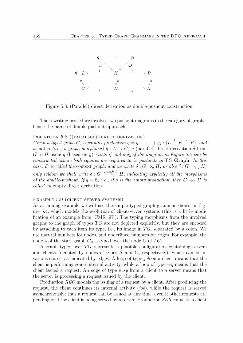
152 Chapter 5. Typed Graph Grammars in the DPO Approach
q1
in1
. . . qk
ink
Lq :
g
Kl r
k
R
h
G Db d
H
Figure 5.3: (Parallel) direct derivation as double-pushout construction.
The rewriting procedure involves two pushout diagrams in the category of graphs,hence the name of double-pushout approach.
Definition 5.8 ((parallel) direct derivation)Given a typed graph G, a parallel production q = q1 + . . .+ qk : (L
l← K
r→ R), and
a match (i.e., a graph morphism) g : L → G, a (parallel) direct derivation δ fromG to H using q (based on g) exists if and only if the diagram in Figure 5.3 can beconstructed, where both squares are required to be pushouts in TG-Graph. In thiscase, D is called the context graph, and we write δ : G⇒q H, or also δ : G⇒q,g H;
only seldom we shall write δ : G〈g,k,h,b,d〉=⇒q H, indicating explicitly all the morphisms
of the double-pushout. If q = ∅, i.e., if q is the empty production, then G ⇒∅ H iscalled an empty direct derivation.
Example 5.9 (client-server systems)As a running example we will use the simple typed graph grammar shown in Fig-ure 5.4, which models the evolution of client-server systems (this is a little modi-fication of an example from [CMR+97]). The typing morphisms from the involvedgraphs to the graph of types TG are not depicted explicitly, but they are encodedby attaching to each item its type, i.e., its image in TG, separated by a colon. Weuse natural numbers for nodes, and underlined numbers for edges. For example, thenode 4 of the start graph G0 is typed over the node C of TG.
A graph typed over TG represents a possible configuration containing serversand clients (denoted by nodes of types S and C, respectively), which can be invarious states, as indicated by edges. A loop of type job on a client means that theclient is performing some internal activity, while a loop of type req means that theclient issued a request. An edge of type busy from a client to a server means thatthe server is processing a request issued by the client.
Production REQ models the issuing of a request by a client. After producing therequest, the client continues its internal activity (job), while the request is servedasynchronously; thus a request can be issued at any time, even if other requests arepending or if the client is being served by a server. Production SER connects a client

5.1. Basic definitions 153
5:S
4:C
0: job
G0
1:S
0:C
0: req0:C
2:S
0:C
2:busy
SER :
1:S
0:C
1:S
0:C
0:busy
1:S
0:C
REL :0:C
0: job0:C 0:C
2: job
1:req
REQ :
S
C
jobreq
busyTG
Figure 5.4: Productions, start graph and graph of types of the grammar C -S mod-elling client-server systems.
that issued a request with a server through a busy edge, modelling the beginning ofthe service. Since the production deletes a node of type S and creates a new one, thedangling condition (see below) ensures that it will be applied only if the server hasno incoming edges, i.e., if it is not busy. Production REL (for release) disconnectsthe client from the server (modelling the end of the service). Notice that in all rulesthe graph morphisms are inclusions.
The grammar is called C -S (for client-server), and it is formally defined asC -S = 〈TG,G0, REQ, SER, REL, π〉, where π maps the production names tothe corresponding production spans depicted in Figure 5.4. 2
To have an informal understanding of the notion of direct derivation, one shouldrecall the interpretation of the pushout as gluing of objects. According to this in-terpretation, the rewriting procedure removes from the graph G the images via g ofthe items of the left-hand side which are not in the image of the interface, namelyg(L− l(K)), producing in this way the graph D. Then the items in the right-handside, which are not in the image of the interface, namely R − r(K), are added toD, obtaining the final graph H . Thus the interface K (common part of L and R)specifies what is preserved. For what regards the applicability of a production to agiven match, it is possible to prove that the situation in the category TG-Graphis exactly the same as in Graph, namely pushouts always exist, while for the exis-tence of the pushout complement some conditions have to be imposed, called gluingconditions [Ehr87], which consist of two parts:
[Dangling condition]No edge e ∈ G− g(L) is incident to any node in g(L− l(K));
[Identification condition]There is no x, y ∈ L, x 6= y, such that g(x) = g(y) and y 6∈ l(K).

154 Chapter 5. Typed Graph Grammars in the DPO Approach
Nicely, the gluing conditions have a very intuitive interpretation: the dangling con-dition avoids the deletion of a node if some edge is still pointing to it, and thus itensures the absence of dangling edges in D. The identification condition requireseach item of G which is deleted by the application of q, to be the image of only oneitem of L. Among other things, this ensures that the application of a productioncannot specify simultaneously both the preservation and the deletion of an item andfurthermore, that a single item of G cannot be deleted “twice” by the applicationof q. Notice that, instead, the identification condition does not forbid the matchto be non-injective on preserved items. Intuitively this means that preserved (read-only) resources can be used with multiplicity greater than one (see [CMR+97] fora broader discussion). Uniqueness of the pushout complement, up to isomorphism,follows from the injectivity of l.
Remark 5.10If G
〈g,k,h,b,d〉⇒∅ H is an empty direct derivation, then morphisms g, k, and h are
necessarily the only morphisms from the empty (typed) graph (since 〈∅, ∅〉 is initialin TG-Graph), while b and d must be isomorphisms. Morphism d b−1 : G→ H iscalled the isomorphism induced by the empty direct derivation. Moreover, for any
pair of isomorphic graphs G ≃ H , there is an empty direct derivation G〈∅,∅,∅,b,d〉⇒∅ H
for each triple 〈D, b : D → G, d : D → H〉, where b and d are isomorphisms. An
empty direct derivation G〈∅,∅,∅,b,d〉⇒∅ H will be also briefly denoted as G
〈b,d〉⇒∅ H . 2
A parallel derivation can be seen as a sequence of single steps of the system, eachone consisting of the concurrent execution of a set of independent basic actions ofthe system, analogously to step sequences of Petri nets.
Definition 5.11 ((parallel) derivation)A (parallel) derivation (over G ) is either a graph G (called an identity derivation,and denoted by G : G ⇒∗ G), or a sequence of (parallel) direct derivations ρ =Gi−1 ⇒qi Gii∈n such that qi = qi1 + . . .+ qiki is a (parallel) production over G forall i ∈ n (as in Figure 5.6). In the last case, the derivation is written ρ : G0 ⇒
∗G Gn
or simply ρ : G0 ⇒∗ Gn. If ρ : G ⇒∗ H is a (possibly identity) derivation, then the
graphs G and H, called the source and target graphs of ρ, are denoted by σ(ρ) andτ(ρ), respectively. The length of a derivation ρ, denoted by |ρ|, is the number of directderivations in ρ (hence |ρ| = 0 if ρ is an identity derivation). The order of ρ, denotedby #ρ, is the total number of elementary productions used in ρ, i.e., #ρ =
∑n
r=1 kr;moreover, prod(ρ) : #ρ → P is the function returning for each j the name of the
j-th production applied in ρ—formally, prod(ρ)(j) = qis if j =(∑i
r=1 kr
)+ s.
The sequential composition of two derivations ρ and ρ′ is defined if and only ifτ(ρ) = σ(ρ′); in this case it is denoted ρ ; ρ′ : σ(ρ) ⇒∗ τ(ρ′), and it is the diagramobtained by identifying τ(ρ) with σ(ρ′) (thus if ρ : G⇒∗ H, then G ; ρ = ρ = ρ ; H,where G and H are the identity derivations).

5.1. Basic definitions 155
5:S
4:C
0: job
G0
5:S
4:C
5:S
4:C
2: job3: req
G1
4:C
2: job
6:S
4:C
6:busy
2: job
G2
6:S
4:C
6:busy
6:S
4:C
6:busy
4: job5: req
G3
6:S
4:C
4: job5: req
6:S
4:C
4: job5: req
G4
1:S
0:C
0: req0:C
2:S
0:C
2:busy
SER :
1:S
0:C
1:S
0:C
0:busy
1:S
0:C
REL :
0:C
0: job0:C 0:C
2: job
1:req
REQ :
0:C
0: job0:C 0:C
2: job
1:req
REQ :
0 - 0 0 - 4 2 - 21 - 3
0 - 40 - 31 - 5
2 - 62 - 6
0 - 2 0 - 42 - 41 - 5
0 - 41 -6
0 - 6
Figure 5.5: A derivation of grammar C -S starting from graph G0.
q11
in1
. . . q1k1
ink
L. . . qis :
insL
K
insK
l rR
insR
. . . qn1
in1
. . . q1kn
ink
L1
g1
K1l1 r1
k1
R1
h1
Ligi
Kili ri
ki
Rihi
Lngn
Knln rn
kn
Rn
hn
G0 D1b1 d1
G1. . . Gi−1 Di
bi diGi . . . Gn−1 Dn
bn dnGn
Figure 5.6: A (parallel) derivation, with explicit drawing of the s-th production ofthe i-th direct derivation.
Example 5.12 (derivation)Figure 5.5 shows a derivation ρ using grammar C -S and starting from the startgraph G0. The derivation models the situation where a request is issued by the client,and while it is handled by the server, a new request is issued. All the horizontalmorphisms are inclusions, while the vertical ones are annotated by the relation ongraph items they induce. 2
5.1.1 Relation with Petri nets
The basic notions introduced so far allow us to give a more precise account of therelation between Petri nets and graph grammars in the double pushout approach.
Being Petri nets one of the most widely accepted models for the representa-tion of concurrent and distributed systems, people working on the concurrencytheory of graph grammars have been naturally led to compare their formalismswith nets. Therefore various encodings of nets into graph graph grammars havebeen proposed along the years, all allowing to have some correspondences between

156 Chapter 5. Typed Graph Grammars in the DPO Approach
t t
C D
A B
D
1
2 1
BA
C
A
(b)(a)
B
2 1
11
A
C D
BA A
A A B B AC B D
[ t >1
Figure 5.7: Firing of a transition and corresponding dpo derivation.
net-related notions and graph-grammars ones. Some encodings involving the dpoapproach can be found in [Kre81, KW86, Sch93] (for a complete survey the readercan consult [Cor96]). All these papers represent a net as a grammar by explicitlyencoding in the start graph the topological structure of the net as well as its initialmarking.
Here we refer to a slightly simpler modelling (see, e.g., [Cor96]), which can helpin understanding how the theory developed in the First Part for contextual andinhibitor nets can be generalized to graph grammars. It is based on the simpleobservation that a Petri net is essentially a rewriting system on multisets, and that,given a set A, a multiset of A can be represented as a discrete graph typed over A.In this view a P/T Petri net can be seen as a graph grammar acting on discretegraphs typed over the set of places, the productions being (some encoding of) thenet transitions: a marking is represented by a set of nodes (tokens) labelled bythe place where they are, and, for example, the unique transition t of the net inFigure 5.7.(a) is represented by the graph production in the top row of Figure 5.7.(b):such production consumes nodes corresponding to two tokens in A and one tokenin B and produces new nodes corresponding to one token in C and one token inD. The interface is empty since nothing is explicitly preserved by a net transition.Notice that in this encoding the topological structure of the net is not representedat all: it is only recorded in the productions corresponding to the transitions.
It is easy to check that this representation satisfies the properties one wouldexpect: a production can be applied to a given marking if and only if the corre-sponding transition is enabled, and the double pushout construction produces thesame marking as the firing of the transition. For instance, the firing of transition t,leading from the marking 3A+ 2B to the marking A+B +C +D in Figure 5.7.(a)becomes the double pushout diagram of Figure 5.7.(b).
The considered encoding of nets into graph grammars enlightens the dimensionsin which graph grammars properly extends nets. First, graph grammars allow fora more structured description of the state, that is a general, possibly non-discrete,graph. Furthermore they allow for productions where the interface graph may notbe empty, thus specifying a “context” consisting of items that have to be present forthe productions to be applied, but are not affected by the application. We already

5.2. Derivation trace semantics 157
observed that, due to their capability of expressing steps which “preserve” part ofthe state, contextual nets can be seen as an intermediate model between ordinaryPetri nets and graph grammars. Indeed, the above encoding of ordinary Petri netsinto graph grammars can be straightforwardly extended to P/T contextual nets.They are represented by graph grammars still acting on discrete graphs, but whereproductions are allowed to have a non-empty interface. Furthermore, we will see inthe next chapter that the graphical structure of the state and the dangling conditionwhich prevents the application of a production when it would leave some danglingedge, has a very natural interpretation in the setting of inhibitor nets.
To conclude, let us stress that a gap of abstraction exists between graph gram-mars and nets. The problem resides in the fact that graphs are more concrete thanmarkings: the nodes of a graph, although carrying the same label, have a preciseidentity, while tokens in the same place of a net are indistinguishable. Formally, theexact counterpart of a marking (multiset) is an isomorphism class of discrete graphs.Therefore suitable equivalences have to be imposed on graphs and derivations if wewant to obtain a precise correspondence with net computations.
5.2 Derivation trace semantics
Historically, the first truly concurrent semantics for graph transformation systemsproposed in the literature has been the derivation trace semantics. It is based onthe idea of defining suitable equivalences on concrete derivations, equating thosederivations which should be considered undistinguishable according to the followingtwo criteria:
• irrelevance of representation details, namely of the concrete identity of theitems in the graphs involved in a derivation, and
• true concurrency, namely irrelevance of the order in which independent pro-ductions are applied in a derivation.
The corresponding equivalences, called respectively abstraction equivalence and shiftequivalence, are presented below. Concatenable derivation traces are then definedas equivalence classes of concrete derivations with respect to the least equivalencecontaining both the abstraction and the shift equivalences. Due to an appropriatechoice of the abstraction equivalence, the obvious notion of sequential compositionof concrete derivations induces an operation of sequential composition at the ab-stract level. Thus, as suggested by their name, concatenable derivation traces canbe sequentially composed and therefore they can be seen as arrows of a category.Such category, called here the category of concatenable derivation traces, coincideswith the abstract truly concurrent model of computation of a grammar presented in[CMR+97], namely the most abstract model in a hierarchy of models of computationfor a graph grammar.

158 Chapter 5. Typed Graph Grammars in the DPO Approach
5.2.1 Abstraction equivalence and abstract derivations
Almost invariably, two isomorphic graphs are considered as representing the samesystem state, which is determined only by the topological structure of the graph andby the typing. This is extremely natural in the algebraic approach to graph transfor-mation, where the result of the rewriting procedure is defined in terms of categoricalconstructions and thus determined only up to isomorphism.2 A natural solution toreason in terms of abstract graphs and abstract derivations consists of consideringtwo derivations as equivalent if the corresponding diagrams are isomorphic. Unfortu-nately, if one wants to have a meaningful notion of sequential composition betweenabstract derivations this approach does not work. For an extensive treatment of thisproblem we refer the reader to [CEL+94b, CEL+94a]. Roughly speaking, the diffi-culty can be described as follows. Two isomorphic graphs, in general, are related bymore than one isomorphism, but if we want to concatenate derivations keeping trackof the flow of causality we must specify in some way how the items of two isomor-phic graphs have to be identified. The problem is treated in [CEL+94b, CEL+94a],which propose a solution based on the choice of a uniquely determined isomorphism,named standard isomorphism, relating each pair of isomorphic graphs.
Here we adopt an equivalent, but slightly different solution which is inspiredby the theory of Petri nets, and in particular by the notion of concatenable netprocess [DMM96], and which borrows a technique from [MSW96]. We choose foreach class of isomorphic typed graphs a specific graph, called canonical graph, andwe decorate the source and target graphs of a derivation with a pair of isomorphismsfrom the corresponding canonical graphs to such graphs. In such a way we are able todistinguish “equivalent”3 elements in the source and target graphs of derivations andwe can safely define their sequential composition. The advantage of our solution isthat the notion of equivalence between derivations does not depend on representationdetails, i.e., on the real identity of the items of the graphs involved in the derivation.For instance, given a derivation, we can change uniformly the name of a node in allthe involved graphs and relations, obtaining a new derivation which is equivalent tothe original one. We refer to [BCE+99] for a more detailed comparison of the twoapproaches.
Definition 5.13 (canonical graphs)We denote by Can a fixed operation that associates to each (TG-typed) graph aso-called canonical graph, satisfying the following properties:
1. Can(G) ≃ G;
2. if G ≃ G′ then Can(G) = Can(G′).
2At the concrete level, the fact that the pushout and pushout complement constructions aredefined only up to isomorphism generates an undesirable and scarcely intuitive unbounded nonde-terminism for each production application.
3With “equivalent” we mean here two items related by an automorphism of the graph, that are,in absence of further information, indistinguishable.

5.2. Derivation trace semantics 159
The construction of the canonical graph can be performed by adapting to our slightlydifferent framework the ideas of [MSW96] and a similar technique can be used tosingle out a class of standard isomorphisms in the sense of [CEL+94b, CEL+94a].Working with finite graphs the constructions are effective.
Definition 5.14 (decorated derivation)A decorated derivation ψ : G0 ⇒
∗ Gn is a triple 〈m, ρ,M〉, where ρ : G0 ⇒∗ Gn is
a derivation, while m : Can(G0)→ G0 and M : Can(Gn)→ Gn are isomorphisms.If ρ is an identity derivation then ψ is called discrete.
In the following we will denote the components of a decorated derivation ψ by mψ,ρψ and Mψ. For a decorated derivation ψ, we write σ(ψ), τ(ψ), #ψ, |ψ|, prod(ψ) torefer to the results of the same operations applied to the underlying derivation ρψ.
Definition 5.15 (sequential composition)Let ψ and ψ′ be two decorated derivations such that τ(ψ) = σ(ψ′) and Mψ = mψ′ .Their sequential composition, denoted by ψ ; ψ′, is defined as follows:
〈mψ, ρψ ; ρψ′ ,Mψ′〉.
One could have expected sequential composition of decorated derivations ψ andψ′ to be defined whenever τ(ψ) ≃ σ(ψ′), regardless of the concrete identity of theitems in the two graphs. We decided to adopt a more concrete notion of concate-nation since it is technically simpler and it induces, like the more general one, thedesired notion of sequential composition at the abstract level.
The abstraction equivalence identifies derivations that differ only for represen-tation details. As announced it is a suitable refinement of the natural notion ofdiagram isomorphism.
Definition 5.16 (abstraction equivalence)Let ψ and ψ′ be two decorated derivations, with ρψ : G0 ⇒
∗ Gn and ρψ′ : G′0 ⇒∗ G′n′
(whose ith steps are depicted in the low rows of Figure 5.8). Suppose that qi =qi1 + . . . + qiki for each i ∈ n, and q′j = q′j1 + . . . + q′jk′j
for each j ∈ n′. Then they
are abstraction equivalent, written ψ ≡abs ψ′, if
1. n = n′, i.e., they have the same length;
2. for each i ∈ n, ki = k′i and for all s ∈ ki, qis = q′is; i.e., the productions appliedin parallel at each direct derivation are the same and they are composed in thesame order; in particular #ψ = #ψ′;
3. there exists a family of isomorphisms
θXi : Xi → X ′i | X ∈ L,K,R,G,D, i ∈ n ∪ θG0
between corresponding graphs appearing in the two derivations such that

160 Chapter 5. Typed Graph Grammars in the DPO Approach
Lis
insL
in′sL
Kis
insKin′sK
Ris
insRin′sR
L′i
g′i
K ′i
k′i
R′i
h′i
Li
θLi
gi
Ki
θKi
ki
Ri
θRi
hi
G′0 G′i D′ib′i d′i
G′i Gn
Can(G0)
m′
m
Can(Gn)
M ′
MG0
θG0
Gi−1
θGi−1
Dibi di
θDi
Gi
θGi
Gn
θGn
Figure 5.8: Abstraction equivalence of decorated derivations (the arrows in produc-tions spans are not labelled).
(a) the isomorphisms relating the source and target graphs commute with thedecorations, i.e., θG0 m = m′ and θGn M = M ′;
(b) the resulting diagram commutes (the middle part of Figure 5.8 representsthe portion of the diagram relative to step i, indicating only the sth of theki productions applied in parallel with the corresponding injections).4
Notice that two derivations are abstraction equivalent if, not only they have thesame length and apply the same productions in the same order, but also, in a sense,productions are applied to “corresponding” items (condition (3)). In other wordsabstraction equivalence identifies two decorated derivations if one can be obtainedfrom the other by uniformly renaming the items appearing in the involved graphs.
Relation ≡abs is clearly an equivalence relation. Equivalence classes of decoratedderivations with respect to ≡abs are called abstract derivations and are denoted by[ψ]abs, where ψ is an element of the class.
It is easy to prove that if ψ ≡abs ψ′ and ψ1 ≡abs ψ′1 then, if defined, ψ;ψ1 ≡
abs
ψ′;ψ′1. Therefore sequential composition of decorated derivations lifts to compositionof abstract derivations.
Definition 5.17 (category of abstract derivations)The category of abstract derivations of a grammar G , denoted by Abs[G ], hasabstract graphs as objects, and abstract derivations as arrows. In particular, ifψ : G ⇒∗ H, then [ψ]abs is an arrow from [G] to [H ]. The identity arrow on [G]is the abs-equivalence class of a discrete derivation 〈i, G, i〉, where i : Can(G)→ Gis any isomorphism, and the composition of arrows [ψ]abs : [G] → [H ] and
4Notice that the isomorphisms θXifor X ∈ L,K,R, relating corresponding parallel produc-
tions, are uniquely determined by the properties of coproducts.

5.2. Derivation trace semantics 161
[ψ′]abs : [H ] → [X] is defined as [ψ ; ψ′′]abs : [G] → [X], where ψ′′ ∈ [ψ′]abs issuch that the composition is defined.
It is worth stressing that, whenever τ(ψ) ≃ σ(ψ′), we can always rename theitems in the graphs of ψ′, in order to obtain a derivation ψ′′, abs-equivalent to ψ′
and composable with ψ, namely such that τ(ψ) = σ(ψ′′) and Mψ = mψ′′ . Basically,it suffices to substitute in the derivation ψ′ each item x in σ(ψ′) with Mψ(m−1
ψ′ (x)).
5.2.2 Shift equivalence and derivation traces
From a truly concurrent perspective two derivations should be considered as equiv-alent when they apply the same productions to the “same” subgraph of a certaingraph, even if the order in which the productions are applied may be different. Thebasic idea of equating derivations which differ only for the order of independentproduction applications is formalized in the literature through the notion of shiftequivalence [Kre77, Kre87, Ehr87]. The shift equivalence is based on the possibil-ity of sequentializing a parallel direct derivation (analysis construction) and on theinverse construction (synthesis construction), which is possible only in the case ofsequential independence. The union of the shift and abstraction equivalences willyield the (concatenable) truly concurrent equivalence, whose equivalence classes arethe (concatenable) derivation traces.
Let us start by defining the key notion of sequential independence. Intuitively,two consecutive direct derivations G ⇒q′ X and X ⇒q′′ H , as in Figure 5.9, aresequentially independent if they may be swapped, i.e., if q′′ can be applied to G,and q′ to the resulting graph, without changing in an “essential way” the matches.Therefore q′′ cannot delete anything that has been explicitly preserved by the ap-plication of q′ at match g1 and, moreover, it cannot use (neither consuming norpreserving it) any element generated by q′; this is ensured if the overlapping of R1
and L2 in X is included in the intersection of the images of the interface graphs K1
and K2 in X.
Definition 5.18 (sequential independence)Consider a derivation δ1; δ2, consisting of two direct derivations δ1 : G⇒q′,g1 X andδ2 : X ⇒q′′,g2 H (as in Figure 5.9). The derivations δ1 and δ2 are called sequentiallyindependent if g2(L2)∩h1(R1) ⊆ g2(l2(K2))∩h1(r1(K1)); in words, if the images inX of the left-hand side of q′′ and of the right-hand side of q′ overlap only on itemsthat are preserved by both derivation steps. In categorical terms, this condition canbe expressed by requiring the existence of two arrows s : L2 → D1 and u : R1 → D2
such that d1 s = g2 and b2 u = h1.
Notice that, differently from what happens for other formalisms, such as ordinaryPetri nets or term rewriting, two rewriting steps δ1 and δ2 do not need to be appliedat completely disjoint matches to be independent. The graphs to which δ1 and δ2are applied can indeed overlap on something that is preserved by both rewriting
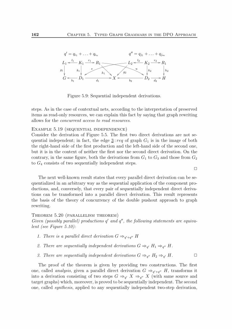
162 Chapter 5. Typed Graph Grammars in the DPO Approach
L1
g1
K1
q′ = qi1 + . . .+ qin
l1 r1
k1
R1
u
h1
L2
sg2
K2
q′′ = qj1 + . . . + qjm
l2 r2
k2
R1
h2
G D1b1 d1
X D2b2 d2
H
Figure 5.9: Sequential independent derivations.
steps. As in the case of contextual nets, according to the interpretation of preserveditems as read-only resources, we can explain this fact by saying that graph rewritingallows for the concurrent access to read resources.
Example 5.19 (sequential independence)Consider the derivation of Figure 5.5. The first two direct derivations are not se-quential independent; in fact, the edge 3 : req of graph G1 is in the image of boththe right-hand side of the first production and the left-hand side of the second one,but it is in the context of neither the first nor the second direct derivation. On thecontrary, in the same figure, both the derivations from G1 to G3 and those from G2
to G4 consists of two sequentially independent steps.2
The next well-known result states that every parallel direct derivation can be se-quentialized in an arbitrary way as the sequential application of the component pro-ductions, and, conversely, that every pair of sequentially independent direct deriva-tions can be transformed into a parallel direct derivation. This result representsthe basis of the theory of concurrency of the double pushout approach to graphrewriting.
Theorem 5.20 (parallelism theorem)Given (possibly parallel) productions q′ and q′′, the following statements are equiva-lent (see Figure 5.10):
1. There is a parallel direct derivation G⇒q′+q′′ H
2. There are sequentially independent derivations G⇒q′ H1 ⇒q′′ H.
3. There are sequentially independent derivations G⇒q′′ H2 ⇒q′ H. 2
The proof of the theorem is given by providing two constructions. The firstone, called analysis, given a parallel direct derivation G ⇒q′+q′′ H , transforms itinto a derivation consisting of two steps G ⇒q′ X ⇒q′′ X (with same source andtarget graphs) which, moreover, is proved to be sequentially independent. The secondone, called synthesis, applied to any sequentially independent two-step derivation,

5.2. Derivation trace semantics 163
H1 q′′
G
q′
q′′
q′+q′′ H
H2q′
Figure 5.10: Local confluence of independent direct derivations.
transforms it into a parallel direct derivation between the same source and targetgraphs. These constructions, in general nondeterministic, are used to define suitablerelations among derivations (see, e.g., [Kre77, EHKPP91, CMR+97]).
Unlike the original definition of analysis and synthesis, following [CEL+96b], weexplicitly keep track of the permutation of the applied productions induced by theconstructions. Therefore we first introduce some notation for permutations.
Definition 5.21 (permutation)A permutation on the set n = 1, 2, . . . , n is a bijective mapping Π : n → n. Theidentity permutation on n is denoted by Πn
id. The composition of two permutationsΠ1 and Π2 on n, denoted by Π1 Π2, is their composition as functions, while theconcatenation of two permutations Π1 on n1 and Π2 on n2, denoted by Π1 | Π2, isthe permutation on n1 + n2 defined as
Π1 | Π2(x) =
Π1(x) if 1 ≤ x ≤ n1
Π2(x− n1) + n1 if n1 < x ≤ n2
Concatenation and composition of permutations are clearly associative.
Proposition 5.22 (analysis and synthesis)Let ρ : G⇒q H be a parallel direct derivation using q = q1+. . .+qk : (L
l← K
r→ R).
Then for each partition 〈I = i1, . . . , in, J = j1, . . . , jm〉 of k (i.e., I ∪ J = kand I ∩ J = ∅) there is a constructive way—in general nondeterministic—to obtaina sequential independent derivation ρ′ : G ⇒q′ X ⇒q′′ H, called an analysis of ρ,where q′ = qi1 + . . .+ qin, and q′′ = qj1 + . . .+ qjm (see Figure 5.9). If ρ and ρ′ are asabove, we shall write ρ ≡anΠ ρ′, where Π is the permutation on k defined as Π(ix) = xfor x ∈ n, and Π(jx) = n+ x for x ∈ m.
Conversely, let ρ : G ⇒q′ X ⇒q′′ H be a pair of sequentially independentderivations. Then there is a constructive way to obtain a parallel direct derivationρ′ = G ⇒q′+q′′ H, called a synthesis of ρ. In this case, we shall write ρ ≡synΠ ρ′,
where Π = Π#ρid . 2
Informally, two derivations are shift equivalent if one can be obtained from theother by repeatedly applying the analysis and synthesis constructions. The next defi-nition emphasizes the fact that the sets of productions applied in two shift equivalent

164 Chapter 5. Typed Graph Grammars in the DPO Approach
derivations are related by a permutation which is constructed inductively startingfrom the permutations introduced by analysis and synthesis.
Definition 5.23 (shift equivalence)Derivations ρ and ρ′ are shift equivalent via permutation Π, written ρ ≡shΠ ρ′, if thiscan be deduced by the following inference rules:
(SH−id)ρ ≡sh
Π#ρid
ρ(SH−∅)
d b−1 = idG
G ≡sh∅ G〈∅,∅,∅,b,d〉⇒∅ G
(SH−an)ρ ≡anΠ ρ′
ρ ≡shΠ ρ′
(SH−syn)ρ ≡synΠ ρ′
ρ ≡shΠ ρ′(SH−sym)
ρ ≡shΠ ρ′
ρ′ ≡shΠ−1 ρ(SH−trans)
ρ ≡shΠ ρ′, ρ′ ≡shΠ′ ρ′′
ρ ≡shΠ′Π ρ′′
(SH−comp)ρ1 ≡
shΠ1ρ′1, ρ2 ≡
shΠ2ρ′2, τ(ρ1) = σ(ρ2)
ρ1 ; ρ2 ≡shΠ1|Π2
ρ′1 ; ρ′2
Note that by (SH− ∅) an empty direct derivation is shift equivalent to the iden-tity derivation G if and only if the induced isomorphism is the identity. The shiftequivalence is the equivalence relation ≡sh defined as ρ ≡sh ρ′ iff ρ ≡shΠ ρ′ for somepermutation Π.
It is worth stressing that the shift equivalence abstracts both from the order inwhich productions are composed inside a single direct parallel step and from theorder in which independent productions are applied at different direct derivations.
Example 5.24 (shift equivalence)Figure 5.11 shows a derivation ρ′ which is shift equivalent to derivation ρ of Figure5.6. It is obtained by applying the synthesis construction to the sub-derivation of ρfrom G1 to G3. 2
Despite the unusual definition, it is easy to check that the shift equivalence justintroduced is the same as in [Kre77, Ehr87, CEL+94a]. From the definitions of theshift equivalence and of the analysis and synthesis constructions, it follows thatρ ≡sh ρ′ implies that ρ and ρ′ have the same order and the same source and targetgraphs (i.e., #ρ = #ρ′, σ(ρ) = σ(ρ′), and τ(ρ) = τ(ρ′); by the way, this guaranteesthat rules (SH− comp) and (SH− trans) are well-defined. The shift equivalence canbe extended in a natural way to decorated derivations.
Definition 5.25The shift equivalence on decorated derivations, denoted with the same symbol ≡sh,is defined by 〈m, ρ,M〉 ≡sh 〈m, ρ′,M〉 if ρ ≡sh ρ′.

5.2. Derivation trace semantics 165
5:S
4:C
0: job
G0
5:S
4:C
5:S
4:C
2: job3: req
G1
6:S
4:C
6:busy
4: job5: req
G3
6:S
4:C
4: job5: req
6:S
4:C
4: job5: req
G4
1:S
0:C
1:S
0:C
0:busy
1:S
0:C
REL =
0:C
0: job0:C 0:C
2: job
1:req
REQ =
0-0 0-4 2-21-3
0-41-6
0-60 - 23 - 3
0 - 41 - 52 - 5
1 - 52 - 45 - 63 - 6
0:C
0: job
1:S
2:C
3: req
0:C
2: job
1:req3:S
2:C
5:busy
0:C
2:C
SER + REQ =
4:C
Figure 5.11: A derivation ρ′ in grammar C -S , shift-equivalent to derivation ρ ofFigure 5.6.
Equivalence ≡sh does not subsume abstraction equivalence, since, for example, itcannot relate derivations starting from different but isomorphic graphs.
We introduce a further equivalence on decorated derivations, obtained simply asthe union of ≡abs and ≡sh. It is called truly-concurrent (or tc-) equivalence, since itequates all derivations which are not distinguishable from a true concurrency per-spective, at an adequate degree of abstraction from representation details. A smallvariation of this equivalence is introduced as well, called ctc-equivalence, where thefirst “c” stays for “concatenable”. Equivalence classes of (c)tc-equivalent decoratedderivations are called (concatenable) derivation traces.
Definition 5.26 (truly-concurrent equivalences and traces)Two decorated derivations ψ and ψ′ are ctc-equivalent via permutation Π, writtenψ ≡cΠ ψ
′, if this can be deduced by the following inference rules:
(CTC−abs)ψ ≡abs ψ′
ψ ≡cΠ#ψid
ψ′(CTC−sh)
ψ ≡shΠ ψ′
ψ ≡cΠ ψ′(CTC−trans)
ψ ≡cΠ ψ′ ψ′ ≡cΠ′ ψ′′
ψ ≡cΠ′Π ψ′′
Equivalence ≡c, defined as ψ ≡c ψ′ iff ψ ≡cΠ ψ′ for some permutation Π, is called the
concatenable truly concurrent (ctc-) equivalence. Equivalence classes of derivationswith respect to ≡c are denoted as [ψ]c and are called concatenable derivation traces.A derivation trace is an equivalence class of derivations with respect to the truly-concurrent (tc-) equivalence ≡ defined by the following rules:
(TC−ctc)ψ ≡cΠ ψ
′
ψ≡Πψ′
(TC−iso)ψ≡Πψ
′ α discrete decor. deriv. s.t. ψ′ ; α is defined
ψ≡Πψ′ ; α
Equivalently, the tc-equivalence could have been defined as ψ ≡Π ψ′ if and only ifψ ≡cΠ 〈mψ′ , ρψ′ ,M ′〉, for some isomorphism M ′ : Can(τ(ψ′)) → τ(ψ′). Informally,

166 Chapter 5. Typed Graph Grammars in the DPO Approach
differently from ctc-equivalence, tc-equivalence does not take into account the dec-orations of the target graphs of derivations, that is their ending interface, and thisis the reason why derivation traces are not concatenable.
Concatenable derivation traces, instead, are naturally equipped with an opera-tion of sequential composition, inherited from concrete decorated derivations, whichallows us to see them as arrows of a category having abstract graphs as objects.Such category is called the category of concatenable derivation traces (or the ab-stract truly concurrent model of computation) of the grammar.
Definition 5.27 (category of concatenable derivation traces)The category of concatenable derivation traces of a grammar G , denoted by Tr[G ],is the category having abstract graphs as objects, and concatenable derivation tracesas arrows. In particular, if ψ : G⇒∗G H then [ψ]c is an arrow from [G] to [H ]. Theidentity arrow on [G] is the ctc-equivalence class of a discrete derivation 〈i, G, i〉,where i is any isomorphism from Can(G) to G. The composition of arrows [ψ]c :[G]→ [H ] and [ψ′]c : [H ]→ [X] is defined as [ψ ; ψ′′]c : [G]→ [X], where ψ′′ ∈ [ψ′]cis a decorated derivation such that ψ ; ψ′′ is defined.
Category Tr[G ] is well-defined because so is the sequential composition of arrows:in fact, if ψ1 ≡
c ψ2 and ψ′1 ≡c ψ′2 then (if defined) ψ1 ; ψ′1 ≡
c ψ2 ; ψ′2 (hence theattribution “concatenable”). Moreover, for abstract derivations, whenever τ(ψ) ≃σ(ψ′), it is always possible to concatenate the corresponding traces, namely one canalways find a derivation ψ′′ ∈ [ψ′]c such that ψ ; ψ′′ is defined.
5.3 A category of typed graph grammars
Various notions of morphism for graph grammars have been introduced in the lit-erature (see, e.g., [CEL+96a, HCEL96, Rib96, BC96]), most of them influenced byWinskel’s notion of Petri net morphism [Win87a, Win87b] through the close rela-tionship existing between typed graph grammars and P/T Petri nets.
Relying on the proposals in [CEL+96a, BC96], this section defines the categoryof graph grammars which will be used in the thesis. We explain how graph grammarsmorphisms arise as a generalization of Petri net morphisms, and we show that, as forPetri nets, graph grammars morphisms preserve the behaviour, namely they allowto “translate” each derivation of the source grammar into a derivation of the targetgrammar.
5.3.1 From multirelations to spans
Multisets and multirelations play an essential role in the definition of morphismsof (generalized) Petri nets. We next provide a categorical view of such concepts, byshowing that a tight relationship exists between the category of multirelations andthe category of spans over Set. These considerations will be helpful to understand

5.3. A category of typed graph grammars 167
the notion of grammar morphism as a generalization of Petri net morphisms. Thematerial is elaborated partly from [CEL+96a], where the first notion of grammarmorphism have been introduced and partly from [BC96, BG00].
The category of spans
We start by reviewing the definition of the category of semi-abstract spans over agiven category [BC96].
Definition 5.28 (span)Let C be a category. A (concrete) span in C is a pair of coinitial arrows f = 〈fL, fR〉with fL : xf → a and fR : xf → b. Objects a and b are called the source an thetarget of the span and we write f : a↔ b. The span f will be sometimes written as〈fL, xf , f
R〉, explicitly giving the object xf .
Consider the relation ∼ over the set of spans of a category, defined as follows:given two spans with the same source and target f, f ′ : a ↔ b, put f ∼ f ′ if thereexists an isomorphism k : xf → xf ′ such that f ′L k = fL and f ′R k = fR (seeFigure 5.12.(a)). It is immediate to see that ∼ is an equivalence relation, whichintuitively abstracts out from the particular choice of the object xf in a concretespan f . The ∼-equivalence class of a concrete span f will be denoted by [f ] andcalled a semi-abstract span.
Definition 5.29 (composition of spans)Let f1 and f2 be spans in a category C. A composition of f1 and f2, denoted by f1; f2
is a span f constructed as in Figure 5.12.(b) (i.e., fL = fL1 y and fR = fR2 z),where the square is a pullback.
The composition of spans is defined only up to equivalence, since the pullback, if itexists, is unique only up to isomorphism. To obtain a categorical structure we mustwork with semi-abstract spans, in a category with pullbacks.
Definition 5.30 (category of spans)Let C be a category with pullbacks. Then the category Span(C) has the same objectsof C and semi-abstract spans on C as arrows. More precisely, a semi-abstract span[f ] is an arrow from the source to the target of f . The composition of two semi-abstract spans [f1] : a↔ b and [f2] : b↔ c is defined as [f1; f2], where f1; f2 denotesany composition of the concrete spans f1 and f2. The identity on an object a is theequivalence class of the span 〈ida, ida〉, where ida is the identity of a in C.
By exploiting the properties of pullbacks it can be shown that Span(C) is a well-defined category, namely that composition is associative and that identities behavecorrectly.

168 Chapter 5. Typed Graph Grammars in the DPO Approach
xf ′f ′L f ′R
a xffL fR
k
b
xfzy
a xf1fL1 fR1
b xf2fL2 fR2
c
(a) (b)
Figure 5.12: Equivalence and composition of spans.
·a1
· ·b1
· ·b2
·a2
· ·b3
·
·a1
·b1
·
· ·b2
·a2
· ·b3
Figure 5.13: The spans f1 (left diagram) and f2 (right diagram) in Set.
Multirelations and Span(Set)
Let us restrict our attention to the category Span(Set) of spans over the categorySet of sets and total functions. We will see that a deep connection exists betweenSpan(Set) and the category MSet of sets and (finitary) multirelations.
Given two sets A and B, consider a semi-abstract span [f ] : A ↔ B. We cangive a graphical representation of a span by tracing an arrow between the elementsx ∈ Xf and a ∈ A whenever fL(x) = a and, similarly, between x ∈ Xf andb ∈ B whenever fR(x) = b. The left diagram in Figure 5.13 represents the span[f1] : A ↔ B, where A = a1, a2, B = b1, b2, b3, Xf = x1, x2, x3 and fR1 =(x1, a1), (x2, a2), (x3, a2), f
L1 = (x1, b1), (x2, b2), (x3, b3). The fact that the set Xf
is fixed only up to isomorphism means that we can disregard the concrete identitiesof its elements.
Intuitively the span is completely characterized by the way in which elements ofA are connected to elements of B. Furthermore observe that not only the existenceof a path between two elements a and b is important, but also the number of suchpaths. For instance the spans f1 and f2 of Figure 5.13 are not equivalent since in f1
the element a1 is connected to b1 via just one path, while in f2 there are two paths.The above discussion suggests that semi-abstract spans in Set can be seen as
an alternative presentation of multirelations, in the sense that one can think of[f ] : A↔ B as specifying for all pairs of elements a ∈ A and b ∈ B, “how many timesthey are related”. For example, the span [f1] can be identified with the multirelation

5.3. A category of typed graph grammars 169
(a1, b1) + (a2, b2) + (a2, b3), while [f2] can be seen as a representation of 2 · (a1, b1) +(a2, b2) + (a2, b3).
This intuitive correspondence can be made very formal. The category MSet ofsets and multirelations can be embedded into Span(Set). The embedding functor isthe identity on objects, and maps any multirelation F : A→ B, which is a functionF : A×B → N, to the span [F ] with
XF = ((a, b), n) | (a, b) ∈ A× B ∧ n < F (a, b)
and FR((a, b), n)) = a, FL((a, b), n)) = b, for all ((a, b), n) ∈ XF .
Proposition 5.31There is an embedding of the category MSet of (finitary) multirelations into thecategory Span(Set) of semi-abstract spans over Set.
The two categories are not isomorphic essentially because Span(Set) extendsMSet by adding also multirelations which are not finitary. Say that a span[f ] : A↔ B is finitary if each element of A has a finite counterimage in Xf , namely
fR−1
(a) is finite for all a ∈ A. Then it is possible to prove that the functor describedabove restricts to an isomorphism between FSpan(Set), the lluf subcategory (Def-inition A.4) of Span(Set) having finitary spans as arrows, and MSet [BG00].
Multisets and multirelation application
Let 1 denote the initial object in Set, namely the set with just one element. Observethat a multiset M of a set A can be seen as a multirelation of 1×A, and therefore itcan be represented as a semi-abstract span [M ] : 1↔ A. Equivalently, since there isa unique arrow from XM to 1, the multiset can be identified with the isomorphism
class of the mapping ML : XM → A (in the comma category 〈Set ↓ A〉). Thisobservation confirms that (abstract) typed graphs are the natural generalization ofmultisets when moving from sets to graphs.
Furthermore, given a multirelation F : A→ B and a multiset M of A, it is im-mediate to verify that the image of M through F , namely µF (M) can be computedsimply as the composition of the corresponding spans, i.e. as M ; F , as depicted inthe left part of Figure 5.14, where the square is a pullback. The arrow towards theinitial object is dotted to stress that we can think of the construction as workingon typed sets. Referring to the figure, we can say that the construction maps the“A-typed set” MR : XM → A to the the “B-typed set” z; FR : XM → A
As an example, the right part of Figure 5.14 shows how the construction can beused to apply the multirelation F1 = 2 ·(a1, b1)+(a2, b2)+(a2, b3), represented by thespan f2 of Figure 5.13, to the multiset a1 + a2. The result is correctly 2 · b1 + b2 + b3.

170 Chapter 5. Typed Graph Grammars in the DPO Approach
1
XM
MR
X
z
y
A XFFRFL
B
a1
a2b2
b3
b1
Figure 5.14: Computing the image of a multiset.
Relations and functions
Relations can be identified with special multirelations R : A → B where multi-plicities are bounded by one (namely R(a, b) ≤ 1 for all a ∈ A and b ∈ B). Thecorresponding condition on a span f : A ↔ B is the existence of at most onepath between any two elements a ∈ A and b ∈ B. The next definition provides acategorical formalization of this concept.
Definition 5.32Let C be a category. A span f : a↔ b in C is called relational if 〈fL, fR〉 : xf → a×bis mono.
In other words f : a ↔ b is relational if given any object c and pair of arrowsg, h : c → xf , if g; fR = h; fR and g; fL = h; fL then g = h. It is easy to verifythat if f : A ↔ B is a span in Set then the above condition can be equivalentlyexpressed as
∀x, y ∈ Xf . fR(x) 6= fR(y) ∨ fL(x) 6= fL(y)
which indeed corresponds exactly to the intuition of having at most one path betweenany two elements. For example, the span f1 of Figure 5.13 is relational, while f2 isnot.
Observe that, in particular, a span f : A ↔ B is relational when either itsleft or right component is injective. It is easy to realize that these kinds of spancorresponds to the partial functions from A to B and backward. In fact, a partialfunction g : A→ B can be identified with the span
A dom(g)g
B
and similarly a partial function h : B → A can be represented as the span
A dom(h)hB
where unlabelled arrows are inclusions.

5.3. A category of typed graph grammars 171
5.3.2 Graph grammar morphisms
Recall that a Petri net morphism [Win87a, Win87b] consists of two components,namely a multirelation between the sets of places and a partial function mappingtransitions of the first net into transitions of the second one. Net morphisms arerequired to “preserve” the pre-set and post-set of transitions, in the sense that thepre- (post-)set of the image of a transition t must be the image of the pre- (post-)setof t.
Since the items of the graph of types of a grammar can be seen as a generalizationof Petri net places, the first component of a grammar morphism from G1 to G2 willbe a semi-abstract span between the type graphs of G1 and G2, which, as explainedin the previous subsection, generalizes the notion of multirelation. The idea of usinggraph grammar morphisms based on spans has been first introduced in [CEL+96a],while the introduction of semi-abstract spans is due to [BC96]. Different notionsof morphism for graph grammars use a (partial) function from the type graph ofG1 to the type graph of G2 [HCEL96] or in the converse direction [Rib96]. Sincepartial functions can be represented as (relational) spans, these notions can be seenas instances of the more general definition based on spans (with the advantage ofallowing a simpler composition, not requiring the use of pullbacks).
Let G1 and G2 be two graph grammars and let [fT ] : TG1 ↔ TG2 be asemi-abstract span between the corresponding type graphs, namely an arrow inSpan(Graph). By extending to graphs the construction presented in the previ-ous section for sets (see Figure 5.14), [fT ] allows us to relate TG1-typed graphsto TG2-typed graphs. Let G1 be in TG1-Graph. The graph G1 is transformed, asdepicted in the diagram below, by first taking a pullback (in Graph) of the arrowsfLT : XfT → TG1 and tG1 : |G1| → TG1, and then typing the pullback object overTG2 by using the right part of the span fRT : XfT → TG2.
|G1|
tG1
|G2|tG2
x
y
TG1 XfTfLT
fRT
TG2
The TG2-typed graph G2 = 〈|G2|, fRT y〉 obtained with this construction, later
referred to as pullback-retyping construction induced by [fT ], is determined only upto isomorphism. Sometimes we will write fTx, y(G1, G2) (or simply fT (G1, G2) ifwe are not interested in morphisms x and y) to express the fact that G1 and G2 arerelated in this way by the pullback-retyping construction induced by [fT ].
We are now ready to define grammar morphisms. Besides the component spec-ifying the relation between the type graphs, a morphism from G1 to G2 contains a(partial) mapping between production names. Furthermore a third component ex-plicitly relates the (untyped) graphs underlying corresponding productions of thetwo grammars, as well as the graphs underlying the start graphs.

172 Chapter 5. Typed Graph Grammars in the DPO Approach
Definition 5.33 (typed graph grammar morphism)Let Gi = 〈TGi, Gsi, Pi, πi〉 (i ∈ 1, 2) be two graph grammars. A (typed graphgrammar) morphism f : G1 → G2 is a triple 〈[fT ], fP , ιf 〉 where
• [fT ] : TG1 → TG2 is a semi-abstract span in Graph, called the type-span;
• fP : P1 → P2 ∪ ∅ is a total function, where ∅ is a new production name(not in P2), with associated production ∅ ← ∅ → ∅, referred to as the emptyproduction;
• ιf is a family ιf(q1) | q1 ∈ P1 ∪ ιsf such that ιsf : |Gs2| → |Gs1| and for
each q1 ∈ P1, if fP (q1) = q2, then ιf (q1) is a triple of morphisms
〈ιLf (q1) : |Lq2 | → |Lq1|, ιKf (q1) : |Kq2| → |Kq1|, ι
Rf (q1) : |Rq2| → |Rq1|〉.
such that the following conditions are satisfied:
1. Preservation of the start graph.There exists a morphism k such that fTι
sf , k(Gs1, Gs2), namely such that the
following diagram commutes (where the square is required to be a pullback).
|Gs1|
tGs1
|Gs2|tGs2
ιsf
k
TG1 XfTfLT
fRT
TG2
2. Preservation of productions.For each q1 ∈ P1, with q2 = fP (q1), there exist morphisms kL, kK and kR
such that the diagram below commutes, and fTιXf (q1), k
X(Xq1, Xq2) for X ∈L,K,R.
|Rq1|
tRq1
|Rq2|ιRf
(q1)
kRtRq2
|Kq1|
tKq1
|Kq2|ιKf
(q1)
kKtKq2
|Lq1|
tLq1
|Lq2 |ιLf(q1)
kL tLq2
TG1 XfTfLT fRT
TG2

5.3. A category of typed graph grammars 173
The grammar morphisms in [CEL+96a] rely on the assumption of having a fixedchoice of pullbacks. Consequently the pullback-retyping construction is deterministicand morphisms are required to preserve the start graphs and the productions “onthe nose”, namely the construction applied to the start graph of G1 must resultexactly in the start graph of G2. Similarly, each production in G1 must be mappedexactly to the corresponding production in G2. Notice that this requirement is verystrict and it may imply the absence of a morphism between two grammars havingstart graph and productions which are the same up to isomorphism. Our notion ofmorphism is, in a sense, more liberal: we avoid a global choice of pullbacks and wefix “locally”, for each morphism f , only part of the pullback diagrams, namely themorphisms in the family ιf . The presence of such component in the morphism isintuitively motivated by the fact that graph grammars are more concrete than Petrinets. In fact, in a graph grammar the start graph and the productions are specifiedby means of concrete graphs, while the initial marking and the transitions of aPetri net are defined in terms of multisets which corresponds to abstract (discrete)graphs. Therefore when a grammar G1 simulates another grammar G2 it is importantto specify not only that a production q1 of G1 is mapped to a production q2 of G2,but also the correspondence between the concrete items of the graphs in the twoproductions q1 and q2.
It is worth noticing that, for technical convenience, the partial mapping on pro-duction names is represented as a total mapping by enriching the target set with adistinguished point ∅, representing “undefinedness”. In this way the condition ask-ing the preservation of productions (condition (2)) faithfully rephrases the situationof net theory where the pre- and post-set of a transition on which the morphism isundefined are necessarily mapped to the empty multiset.
Definition 5.34 (category GG)Graph grammars and graph grammar morphisms form a category GG.
The identities and the composition of morphisms in GG are defined in the obviousway. Given a grammar G , the identity on G is the grammar morphism 〈[idTG], idP , ι〉,where [idTG] is the identity span on TG, idP is the identity function on P and allthe components of ι are identities on the corresponding graphs.
Given two morphisms f0 : G0 → G1 and f1 : G1 → G2, the composition f1 f0 :G0 → G2 is the morphism 〈[f1T ] [f0T ], f1P f0P , ι〉, where for any q0 ∈ P0 and anyX ∈ L,K,R, we have ιX(q0) = ιXf0(q0) ι
Xf1
(f0P (q0))
5.3.3 Preservation of the behaviour
As in [CEL+96a] it is possible to show that morphisms preserve the behaviour ofgraph grammars, in the sense that given a morphism f : G1 → G2, for every deriva-tion ρ1 in G1 there is a corresponding derivation ρ2 in G2, related to ρ1 by thepullback-retyping construction induced by the type component [fT ] of the morphism.

174 Chapter 5. Typed Graph Grammars in the DPO Approach
First, we need to review some results expressing properties of pullbacks andpushouts in Graph. The properties are stated for the category Set of sets and totalfunctions, since the constructions of pullback and pushout can be lifted from Set toGraph, where limits and colimits are constructed “componentwise”. A proof canbe found in [CEL+96a].
Proposition 5.35Consider the following commuting diagram in Set
A B
C
PB
PB
D
E F
If the two internal squares, marked by PB are pullbacks, then the outer square withvertices A, B, E and F is a pullback as well.
Proposition 5.36 (3-cube lemma)Consider the following commuting diagram in Set
A B
E
PB
PB PO
F
G
PB
H
PB
C D
If the small internal squares, marked by PB and PO are pullbacks and pushouts,respectively, then the outer square with vertices A, B, C and D is a pushout.
We are now ready to prove that graph grammar morphisms preserve derivations.As a consequence of the partial arbitrariness in the choice of the pullback com-ponents, such correspondence is not “functional”, but it establishes just a relationbetween concrete derivations of the source and target grammars of the morphism.
Lemma 5.37Let f : G1 → G2 be a graph grammar morphism, and let δ1 : G1 ⇒
∗q1H1 be a direct
derivation in G1. Then there exists a corresponding direct derivation δ2 : G2 ⇒∗fP (q1)
H2 in G2, such that fT (G1, G2) and fT (H1, H2).
Proof. The proof is extremely technical and follows the same outline as in [CEL+96a]. Here wegive only a sketch, singling out some relevant passages.
Assume that the derivation δ1 in G1 has the following shape:

5.3. A category of typed graph grammars 175
L1q1 :
g1
K1
k1
R1
h1
G1 D1b1 d1
H1
The same derivation is depicted also in the left part of Figure 5.15. The right part of the top layerrepresents the production q2 = fP (q1). Observe that the figure is not complete. First, for eachgraph appearing in the top layer we should have indicated the corresponding typing morphism.Furthermore, by definition of grammar morphism, the two productions q1 and q2 are related by apullback-retyping construction as expressed by condition (3) in Definition 5.33, and thus a mor-phism κY : |Y2| → X should appear for Y ∈ L,K,R. For the sake of clearness only the typingmorphisms of L1 and and the morphism kL : |L2| → X of the pullback-retyping construction areexplicitly represented.
Consider any three graphs G2, D2 and H2, obtained from G2, D2 and H2, respectively, by ap-plying the pullback-retyping construction. Such graphs, with the corresponding pullback-retypingdiagrams are represented in the bottom part of Figure 5.15. Now, recall that the square with ver-tices |G1|, |G2|, TG1, X is a pullback, and the square with vertices |L1|, |L2|, TG1, X commutes.Hence the match g2 : |L2| → |G2| is uniquely determined by the universal property of pullbacks.Similarly, observing that the square |D1|, |D2|, TG1, X , commutes we uniquely determine a mor-phism b2 : |D2| → |G2|. With an analogous reasoning we can complete the whole diagram ofFigure 5.15.
By using Proposition 5.35 it is not difficult to realize that all the squares with vertices
• |L1|, |L2|, |G1|, |G2| • |D1|, |D2|, |K1|, |K2|• |G1|, |G2|, |D1|, |D2| • |K1|, |K2|, |L1|, |L2|
are pullbacks, while the square |K1|, |L1|, |G1|, |D1| is a pushout, by construction. By the 3-cubelemma (Proposition 5.36) we deduce that the square |K2|, |L2|, |G2|, |D2| is a pushout. Since, bysymmetry also |K2|, |D2|, |H2|, |R2| is a pushout, this concludes the construction of the desireddirect derivation δ2.
2
The result can straightforwardly be extended to general derivations involving anarbitrary number of (possibly parallel) direct derivation.
Recall that in [CEL+96a], where the more concrete notion of morphism based ona choice of pullbacks is adopted, the relation between derivations induced by a mor-phism is indeed a function. Furthermore the result above is extended to show that theconcrete model of computation of the grammar (not considering abstraction equiv-alence) can be obtained via a functorial construction, establishing an adjunctionbetween the category of graph grammars and the category of concrete derivations.

176 Chapter 5. Typed Graph Grammars in the DPO Approach
|R1|
h1
|R2|ιRf
(q1)
h2
|K1|
k1
|K2|ιKf
(q1)
k2
|H1| |H2|
|L1|
tL1
g1
|L2|ιLf(q1)
g2
κL
|D1|
b1
d1
|D2|
b2
d2
|G1| |G2|
TG1 XfLT fRT
TG2
Figure 5.15: Graph grammars morphisms preserve derivations.

Chapter 6
Unfolding and Event StructureSemantics
This chapter introduces a truly concurrent semantics for dpo graph grammars basedon a Winskel-style unfolding construction. The work developed in the First Partfor contextual and inhibitor nets represents both an intuitive guide and a formal basisfor the treatment of graph grammars. In fact, as in contextual nets, the possibilityof specifying rewriting steps which preserve part of the state leads to asymmetricconflicts between productions. Furthermore the dangling condition, a part of theapplication condition which prevents the application of a production when it wouldleave dangling edges, has a natural encoding in the setting of inhibitor nets: the edgeswhose presence prevents the application of a production can be seen as inhibitorplaces for that production.
First, nondeterministic occurrence grammars, which generalize the (determin-istic) occurrence grammars of [CMR96], are defined as safe grammars satisfyingsuitable acyclicity and well-foundedness conditions. As occurrence inhibitor nets aredefined without considering the inhibitor arcs, the requirements on occurrence gram-mars disregard the constraints imposed by the dangling condition. Consequently notall the productions of an occurrence grammar are really executable. The possibledeterministic computations of an occurrence grammar are captured by consideringthe configurations of the grammar which are later shown to be closely related to theconfigurations of the corresponding event structure.
An unfolding construction is proposed, which associates to each (consuming)graph grammar a nondeterministic occurrence grammar representing its behaviour.As for nets, the idea consists of starting from the start graph of the grammar,applying in all possible ways the productions of the grammar, and recording in theunfolding each occurrence of production and each new graph item generated by therewriting process, both enriched with the corresponding causal history. Consistentlywith the notion of occurrence grammar, in the construction of the unfolding theproductions are applied without considering the dangling condition.
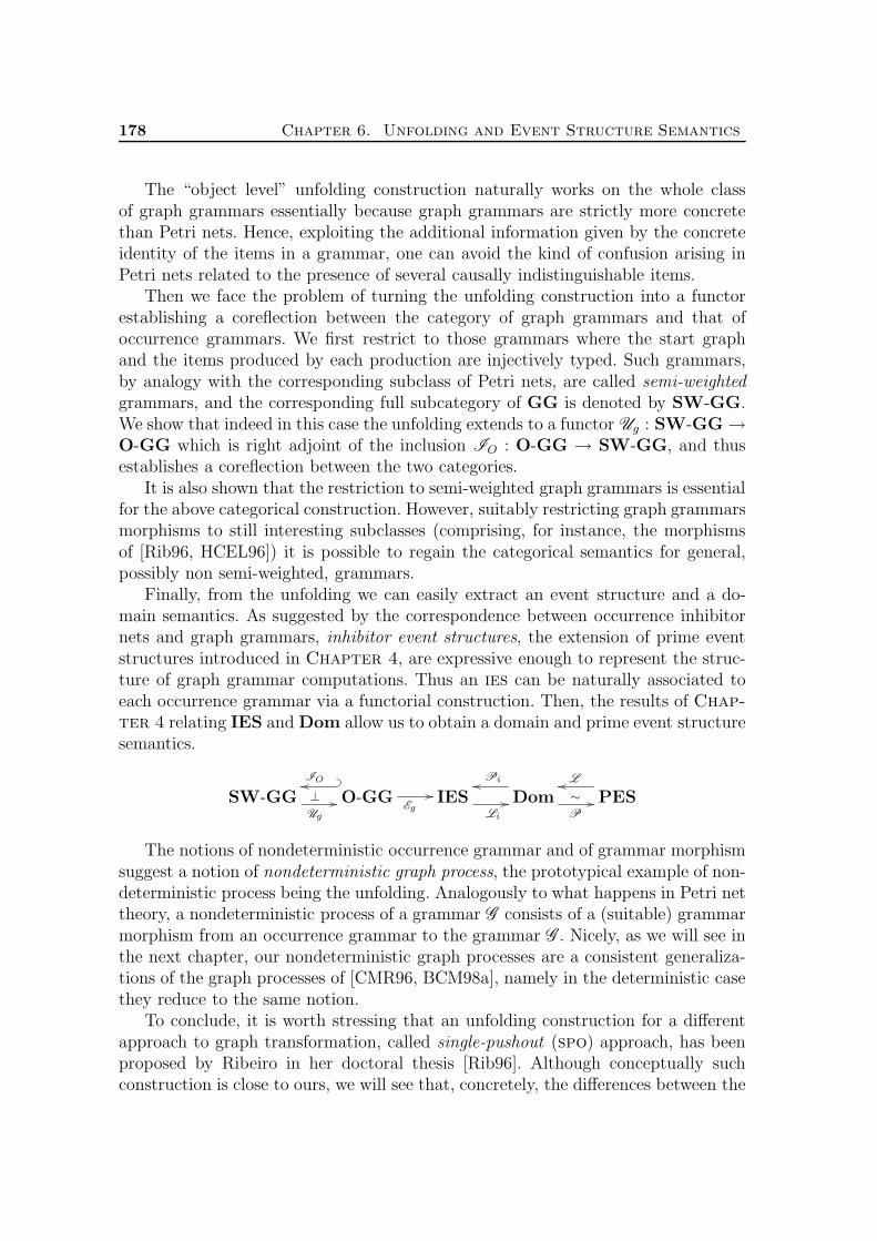
178 Chapter 6. Unfolding and Event Structure Semantics
The “object level” unfolding construction naturally works on the whole classof graph grammars essentially because graph grammars are strictly more concretethan Petri nets. Hence, exploiting the additional information given by the concreteidentity of the items in a grammar, one can avoid the kind of confusion arising inPetri nets related to the presence of several causally indistinguishable items.
Then we face the problem of turning the unfolding construction into a functorestablishing a coreflection between the category of graph grammars and that ofoccurrence grammars. We first restrict to those grammars where the start graphand the items produced by each production are injectively typed. Such grammars,by analogy with the corresponding subclass of Petri nets, are called semi-weightedgrammars, and the corresponding full subcategory of GG is denoted by SW-GG.We show that indeed in this case the unfolding extends to a functor Ug : SW-GG→O-GG which is right adjoint of the inclusion IO : O-GG → SW-GG, and thusestablishes a coreflection between the two categories.
It is also shown that the restriction to semi-weighted graph grammars is essentialfor the above categorical construction. However, suitably restricting graph grammarsmorphisms to still interesting subclasses (comprising, for instance, the morphismsof [Rib96, HCEL96]) it is possible to regain the categorical semantics for general,possibly non semi-weighted, grammars.
Finally, from the unfolding we can easily extract an event structure and a do-main semantics. As suggested by the correspondence between occurrence inhibitornets and graph grammars, inhibitor event structures, the extension of prime eventstructures introduced in Chapter 4, are expressive enough to represent the struc-ture of graph grammar computations. Thus an ies can be naturally associated toeach occurrence grammar via a functorial construction. Then, the results of Chap-ter 4 relating IES and Dom allow us to obtain a domain and prime event structuresemantics.
SW-GGUg
⊥ O-GGEg
IO
IESLi
Dom
Pi
P
∼ PESL
The notions of nondeterministic occurrence grammar and of grammar morphismsuggest a notion of nondeterministic graph process, the prototypical example of non-deterministic process being the unfolding. Analogously to what happens in Petri nettheory, a nondeterministic process of a grammar G consists of a (suitable) grammarmorphism from an occurrence grammar to the grammar G . Nicely, as we will see inthe next chapter, our nondeterministic graph processes are a consistent generaliza-tions of the graph processes of [CMR96, BCM98a], namely in the deterministic casethey reduce to the same notion.
To conclude, it is worth stressing that an unfolding construction for a differentapproach to graph transformation, called single-pushout (spo) approach, has beenproposed by Ribeiro in her doctoral thesis [Rib96]. Although conceptually suchconstruction is close to ours, we will see that, concretely, the differences between the

6.1. Nondeterministic occurrence grammars 179
two settings, like the absence of the application condition in the spo approach, adifferent notion of “enabling” allowing for the concurrent application of productionsrelated by asymmetric conflict and a different choice of grammar morphisms, makesdifficult a direct comparison.
The rest of the chapter is organized as follows. Section 6.1 introduces the no-tion of nondeterministic occurrence grammar and gives some more insights on therelation between graph grammars and inhibitor nets. Relying on the notion of occur-rence grammar, Section 6.2 introduces nondeterministic graph processes. Section 6.3describes the unfolding construction for graph grammars, whose categorical proper-ties are then investigated in Section 6.4. Then Section 6.5 shows how an ies can beextracted from an occurrence grammar, thus providing, through the unfolding con-struction, an event structure semantics for graph grammars. Finally, in Section 6.6we compare the unfolding construction in this chapter with that proposed in [Rib96]for the spo approach.
6.1 Nondeterministic occurrence grammars
A first step towards the definition of nondeterministic occurrence grammars is asuitable notion of safeness for grammars [CMR96], generalizing that for P/T nets,which requires that each place contains at most one token in any reachable marking.
Definition 6.1 ((strongly) safe grammar)A grammar G = 〈TG,Gs, P, π〉 is (strongly) safe if, for all H such that Gs ⇒
∗ H,H has an injective typing morphism.
The definition can be understood by thinking of nodes and edges of the type graphas a generalization of places in Petri nets. In this view the number of different itemsof a graph which are typed on a given item of the type graph corresponds to thenumber of tokens contained in a place, and thus the condition of safeness for amarking is generalized to typed graphs by the injectivity of the typing morphism.
Strongly safe graph grammars (hereinafter called just safe grammars) admit anatural net-like pictorial representation, where items of the type graph and pro-ductions play, respectively, the role of places and transitions of Petri nets. Thebasic observation is that typed graphs having an injective typing morphism can besafely identified with the corresponding subgraphs of the type graph (just thinkingof injective morphisms as inclusions). Therefore, in particular, each graph 〈|G|, tG〉reachable in a safe grammar can be identified with the subgraph tG(|G|) of the typegraph TG, and thus it can be represented by suitably decorating the nodes andedges of TG. Concretely, a node is drawn as a filled circle if it belongs to tG(|G|)and as an empty circle otherwise, while an edge is drawn as a continuous line if it isin tG(|G|) and as a dashed line otherwise (see Figure 6.1). This is analogous to theusual technique of representing the marking of a safe net by putting a token in eachplace which belongs to the marking.

180 Chapter 6. Unfolding and Event Structure Semantics
With the above identification, in each derivation of a safe grammar starting fromthe start graph a production can be applied only to the subgraph of the type graphwhich is the image via the typing morphism of its left-hand side. Therefore accordingto its typing, we can think that a production produces, preserves and consumes itemsof the type graph. This is expressed by drawing productions as arrow-shaped boxes,connected to the consumed and produced resources by incoming and outcomingarrows, respectively, and to the preserved resources by undirected lines. Figure 6.1presents two examples of safe grammars, with their pictorial representation. Noticethat the typing morphisms for the start graph and the productions are representedby suitably labelling the involved graphs with items of the type graph.
Using a net-like language, we speak of pre-set •q, context q and post-set q• ofa production q. The notions of pre-set, post-set and context of a production havea clear interpretation only for safe grammars. However for technical reasons it ispreferable to define them for general graph grammars.
Definition 6.2 (pre-set, post-set, context)Let G be a graph grammar. For any q ∈ P we define
•q = tLq(|Lq| − lq(|Kq|)) q• = tRq(|Rq| − rq(|Kq|))
q = tKq(|Kq|)
seen as sets of nodes and edges, and we say that q consumes, creates and preservesitems in •q, q• and q, respectively. Similarly for a node or an edge x in TG we write•x, x and x• to denote the sets of productions which produce, preserve and consumex, respectively.
For instance, for grammar G2 in Figure 6.1, the pre-set, context and post-set ofproduction q1 are •q1 = C, q1 = B and q1
• = A,L, while for the node B,•B = ∅, B = q1, q2, q3 and B• = q4.
Observe now that because of the dangling condition, a production q which con-sumes a node n can be applied only if there are no edges with source or target in nwhich remain dangling after the application of q. In other words, if n ∈ •q, e 6∈ •qand n ∈ s(e), t(e) then the application of q is inhibited by the presence of e. Byanalogy with inhibitor nets we introduce the inhibitor set of a production.
Definition 6.3 (inhibitor set)Let G be a graph grammar. The inhibitor set of a production q ∈ P is defined by
q = e ∈ ETG | ∃n ∈•q. n ∈ s(e), t(e) ∧ e 6∈ •q
Similarly, for an edge e ∈ ETG we define the inhibitor set of e as the set of produc-tions inhibited by e, namely e = q ∈ P | e ∈ q.
For instance, in the grammar G2 of Figure 6.1 the inhibitor set of q4 is q4 = L,while for the edge L we have L = q4.

6.1. Nondeterministic occurrence grammars 181
Grammar G1
A B B B
TG = Gin =
q3
q2
q1
q1
q3q2
B
A
AL
B
L
BA L
Grammar G2
q4
L
L
A Bq1
q3
TG =
q2
C
L BA
q2 q3
q4
q1
B
AA BBA B
CBA CB
BA
B C B
B B
L
L
Gin =
Figure 6.1: Two safe grammars and their net-like representation.
Note that with the above definition, a production q of a safe grammar G satisfiesthe dangling condition (when using its typing as match) in a subgraph G of the typegraph TG if and only if q ∩G = ∅.
The correspondence between safe grammars and inhibitor nets can be made moreexplicit by observing that we can associate to any safe grammar G = 〈Gs, TG, P, π〉an inhibitor net NG having the items of TG as places, Gs as initial marking, P asset of transitions with pre-set, post-set, context and inhibitor set of each transitiondefined exactly as in the grammar. Figure 6.2 shows the inhibitor nets correspondingto the safe grammars G1 and G2 in Figure 6.1. It is possible to show that the gram-mar G and the net NG have essentially the same behaviour in the sense that eachderivation in G corresponds to a step sequence in NG using the same productions andleading to the same state, and vice versa. Although this fact is not used in a formalway, the proposed translation can help in understanding how the work on contextualand inhibitor nets influences the treatment of graph grammars in this chapter. Itis important to observe that the inhibitor net associated to a safe graph grammarby the described translation has a very particular shape, as expressed below.

182 Chapter 6. Unfolding and Event Structure Semantics
•
A
q3 •
L
q1 •
B
q2
•
C
q1L
Aq3 •
B
q2 q4
Figure 6.2: The inhibitor nets corresponding to the grammars G1 and G2 in Fig-ure 6.1.
Remark 6.4Let G be a safe grammar and let q, q′ ∈ P be two productions of G . Observe thatwhenever q• ∩ q′ 6= ∅ then necessarily q ր q′. In fact let e ∈ q• ∩ q′. By definitionof q′ the production q′ consumes a node n which is the source or the target of e.Since, by definition of q•, the production q produces the edge e, it must produce orpreserve the node n. Consequently n ∈ (q• ∪ q) ∩ •q′ and thus q ր q′. For similarreasons, if q′ ∩ •q′′ 6= ∅ then q′′ ր q′.
Hence, differently from what happens in general inhibitor nets, if a production qcan inhibit a production q′ then q cannot be applied after q′. For instance, considerthe net NG2 in the right part of Figure 6.2. The production q1 can inhibit q4 since itproduces a token in L and indeed it must precede q4, since B ∈ q1 ∩
•q4. Similarlyq3 re-enables q4 and q3 ր q4. This means that, in a sense, (safe) graph grammarscomputations are simpler than (safe) inhibitor nets computations.
Following the approach adopted for inhibitor nets, the causal and asymmetricconflict relations for a graph grammar are defined without taking into account theinhibitor sets, namely disregarding the dangling condition.
Definition 6.5 (causal relation)The causal relation of a grammar G is the binary relation < over Elem(G ) definedas the least transitive relation satisfying: for any node or edge x in the type graphTG and for productions q1, q2 ∈ P
1. if x ∈ •q1 then x < q1;
2. if x ∈ q1• then q1 < x;
3. if q1• ∩ q2 6= ∅ then q1 < q2.
As usual ≤ denotes the reflexive closure of <. Moreover, for x ∈ Elem(G ) we write⌊x⌋ for the set of causes of x in P , namely q ∈ P | q ≤ x.

6.1. Nondeterministic occurrence grammars 183
Definition 6.6 (asymmetric conflict)The asymmetric conflict relation of a grammar G is the binary relation ր over theset P of productions, defined by:
1. if q1 ∩•q2 6= ∅ then q1 ր q2;
2. if •q1 ∩•q2 6= ∅ and q1 6= q2 then q1 ր q2;
3. if q1 < q2 then q1 ր q2.
A nondeterministic occurrence grammar is an acyclic grammar which represents,in a branching structure, several possible computations starting from its start graphand using each production at most once. Again the dangling condition is not con-sidered in the definition.
Definition 6.7 ((nondeterministic) occurrence grammar)A (nondeterministic) occurrence grammar is a graph grammar O = 〈TG,Gs, P, π〉such that
1. the causal relation ≤ is a partial order, and for any q ∈ P the set ⌊q⌋ is finiteand the asymmetric conflict ր is acyclic on ⌊q⌋;
2. the start graph Gs coincides with the set Min(O) of the items of the type graphTG which are minimal with respect to causality ≤ (with the graphical structureinherited from TG and typed by the inclusion);
3. each edge or node x in TG is created by at most one production in P , namely| •x| ≤ 1;
4. for each production q : Lqlq← Kq
rq→ Rq, the typing tLq is injective on the
“consumed part” |Lq|− lq(|Kq|), and similarly tRq is injective on the “producedpart” |Rq| − rq(|Kq|).
We denote by O-GG the full subcategory of GG having occurrence grammars asobjects.
Since the start graph of an occurrence grammar O is determined by Min(O), weoften do not mention it explicitly.
Intuitively, conditions (1)–(3) recast in the framework of graph grammars theanalogous conditions of occurrence contextual nets. Condition (4), is closely relatedto safeness and requires that each production consumes and produces items with“multiplicity” one. Observe that, together with acyclicity of ր, it disallows thepresence of some productions which surely could never be applied, because they failto satisfy the identification condition with respect to the typing morphism.

184 Chapter 6. Unfolding and Event Structure Semantics
The next proposition shows that, by the defining conditions, each occurrencegrammar is safe.
Proposition 6.8 (occurrence and safe grammars)Each occurrence grammar O is safe.
Proof. Let O = 〈TG,P, π〉 be an occurrence grammar and let ρ : Gs ⇒∗ Gn be a derivation in O.Since the grammar is consuming, namely each production has a non empty pre-set, and causality≤ is a partial order (there are no “cycles”), every derivation in the grammar starting from thestart graph can apply each production at most once. Without any loss of generality we can assumethat each direct derivation of ρ applies a single production.
We show by induction on the order n of the derivation that the graph Gn is injective. For n = 0just recall that Gs is a subgraph of TG, typed by the inclusion. If n > 0, by inductive hypothesis,Gn−1 is injective. Moreover the typing of qn is injective on |Rqn
| − rqn(|Kqn
|). This observation,together with the fact that the items of the start graph have empty pre-set (they are minimalwith respect to causality) and each item of the type graph is produced by at most one productionimplies that the graph Gn, which is obtained from Gn−1 by first “removing” Lqn
− lqn(Kqn
) andthen “adding” Rqn
− rqn(Kqn
), is injective. 2
Disregarding the dangling condition in the definition of occurrence grammar hasas a consequence the fact that, analogously to what happens for inhibitor nets, weare not guaranteed that every production of an occurrence grammar is applicableat least in one derivation starting from the start graph. The restrictions to thebehaviour imposed by the dangling condition are taken into account when definingthe configurations of an occurrence grammar, which represent exactly, in a senseformalized later, all the possible deterministic runs of the grammar.
Definition 6.9 (configuration)A configuration of an occurrence grammar O = 〈TG, P, π〉 is a subset C ⊆ P suchthat
1. if րC denotes the restriction of the asymmetric conflict relation to C, then(րC)∗ is a finitary partial order on C;
2. C is left-closed with respect to ≤, i.e. for all q ∈ C, q′ ∈ P , q′ ≤ q impliesq′ ∈ C;
3. for all e ∈ TG, if e ∩ C 6= ∅ and •e ⊆ C then e• ∩ C 6= ∅.
If C satisfies conditions (1) and (2), then it is called a pre-configuration. The set ofall configurations of the grammar O is denoted by Conf (O).
Condition (1) ensures that in C there are no ր-cycles and thus it excludes thepossibility of having in C a subset of productions in conflict. Furthermore it guar-antees that each production has to be preceded only by finitely many other pro-ductions in the computation represented by the configuration. Condition (2) re-quires the presence of all the causes of each production. Condition (3) considersthe dangling condition: for any edge e in the type graph, if the configuration con-tains a production q inhibited by e and a production q′ producing such an edge

6.1. Nondeterministic occurrence grammars 185
then some production q′′ consuming e must be present as well, otherwise, due tothe dangling condition, q could not be executed. This requirement is better un-derstood recalling that, as observed in Remark 6.4, in this situation, i.e., whene ∈ q′• ∩ q 6= ∅, necessarily q′ ր q, namely q′ must be applied before q in the com-putation. Similar considerations apply if the edge e is present in the start graph,i.e., •e = ∅. For example the set of configurations of the grammar G2 in Fig-ure 6.1 is Conf (G2) = ∅, q1, q1, q2, q1, q3, q1, q2, q4, q1, q3, q4, q4. Theset S = q1, q4, is instead only a pre-configuration, since for the edge L we haveq4 ∈
L, •L = q1 ⊆ S, but the intersection of S with L• = q2, q3 is empty.The notion is reminiscent of that of configuration of an inhibitor event structure.
Indeed we will prove later that the configurations of an occurrence grammar areexactly the configurations of the ies associated to the grammar. The fact that anoccurrence grammar configuration does not include an explicit choice relation canbe understood, for the moment, by recalling Remark 6.4 which implies that theproductions in a configuration implicitly determine their order of application.
The claim that configurations represent all and only the deterministic runs of anoccurrence grammar is formalized by the following result. We first need the notion ofreachable graph associated to a configuration, which extends an analogous conceptintroduced in [CMR96], in the case of deterministic occurrence grammars.
Definition 6.10 (reachable graphs)Let O = 〈TG, P, π〉 be an occurrence grammar. For any C ⊆ P , finite configurationof O, the reachable set associated to C is the set of nodes and edges reach(C) ⊆Items(TG) defined as
reach(C) = (Min(O) ∪⋃q∈C q
•)−⋃q∈C
•q.
Proposition 6.11 (configurations and derivations)Let C be any configuration of an occurrence grammar O. Then reach(C) is a well-defined subgraph of the type graph TG and, moreover, Min(O) ⇒∗C reach(C) witha derivation which applies exactly once every production in C, in any order con-sistent with (րC)∗. Vice versa for each derivation Min(O) ⇒∗S G in O, the set ofproductions S it applies is a configuration and G = reach(S).
Proof. Let C ∈ Conf (O) be any finite configuration of O. The fact that reach(C) is a well-definedsubgraph of the type graph TG and Min(O)⇒∗
C reach(C) can be proved by induction on |C|. Thebase case in which |C| = 0, namely C = ∅, is trivial since, by definition, Min(O) = reach(∅). Ifinstead |C| > 0 consider any production q ∈ C, maximal with respect to (րC)∗ (such a productionexists since (րC)∗ is a partial order and C is finite). It is easy to see that C−q is a configurationand therefore, by inductive hypothesis,
Min(O)⇒∗C−q G
where G = reach(C − q). By point (1) in the definition of configuration, entailing that րC isacyclic, and by point (2) we immediately get that •q∪ q ⊆ G. Furthermore, by point (3), q∩G =∅ and thus q satisfies also the dangling condition. Recalling that q satisfies the identification

186 Chapter 6. Unfolding and Event Structure Semantics
condition by definition of occurrence grammar, we deduce that q is applicable to G and thusG⇒q (G− •q) ∪ q•. Since in an occurrence grammar the post-sets of productions are all disjointwe conclude that (G− •q) ∪ q• = reach(C) and thus
Min(O)⇒∗C reach(C)
The second part of the proposition can be proved essentially by reversing the above steps. 2
As an immediate consequence of the previous result, a production which doesnot satisfy the dangling condition in any graph reachable from the start graph (andthus which is never applicable) is not part of any configuration. For example, q3 doesnot appear in the set of configurations of G1, Conf (G1) = ∅, q1, q2, q1, q2.
6.2 Nondeterministic graph processes
In the theory of Petri nets the notion of occurrence net is strictly related to thatof process. A (non)deterministic net process is a (non)deterministic occurrence netwith a suitable morphism to the original net. Similarly, nondeterministic occurrencegrammars can be used to define a notion of nondeterministic graph processes, gener-alizing the deterministic graph processes of [CMR96, BCM98a]. Then, the unfoldingof a grammar, as introduced in the next section, can be seen as a “complete” non-deterministic process of the grammar, expressing all the possible computations ofthe grammar.
A nondeterministic graph process is aimed at representing in a unique “branch-ing” structure several possible computations of a grammar. The underlying occur-rence grammar makes explicit the causal structure of such computations since eachproduction can be applied at most once and each item of the type graph can be“filled” at most once. Via the morphism to the original grammar, productions anditems of the type graph in the occurrence grammar can be thought of, respectively,as instances of applications of productions and instances of items generated in theoriginal grammar by such applications. Actually, to allow for such an interpretation,some further restrictions have to be imposed on the process morphism. Recall thatprocess morphisms in Petri net theory must map places to places (rather than tomultisets of places) and must be total on transitions. Similarly, for graph processmorphisms the left component of the type-span is required to be an isomorphism insuch a way that the type-span can be thought of simply as a total graph morphism.Furthermore a process morphism cannot map a production to the empty production,a requirement corresponding to totality.
Definition 6.12 (strong morphism)A grammar morphism f : G1 → G2 is called strong if
1. fLT : XfT → TG1 is an isomorphism;
2. fP (q1) 6= ∅, for any q1 ∈ P1.

6.2. Nondeterministic graph processes 187
|Gsϕ|
tGsϕ
|Gs|ιsϕ
tGs
TGϕϕRT
TG
|R′|
tR′
|R|ιRϕ (q1)
tR
q′ |K ′|
tK′
|K|ιKϕ (q′)
tK
ϕP (q′) = q
|L′|
tL′
|L|ιLϕ(q′)
tL
TGϕϕRT
TG1
Figure 6.3: Graph processes.
In the following, without any loss of generality, we will always choose as concreterepresentative of the type-span of a strong grammar morphism f , a span fT suchthat the left component fLT is the identity idTG1.
Definition 6.13 (graph process)Let G be a graph grammar. A (marked) graph process of G is a strong grammarmorphism ϕ : Oϕ → G , where Oϕ is an occurrence grammar. We will denote byTGϕ, Gsϕ, Pϕ and πϕ the components of the occurrence grammar Oϕ underlying aprocess ϕ.
Alternatively, if GG∗ indicates the subcategory of GG having the same objects andstrong grammar morphisms as arrows, then the category of processes of a grammarG can be simply defined as the comma category 〈O-GG ↓ G 〉 in GG∗.
It is not difficult to verify that, if f : G1 → G2 is a strong morphism then, by con-dition (1) in the definition of grammar morphism (Definition 5.33), ιsf : |Gs2| → |Gs1|is an isomorphism. Similarly, by condition (2), for each production q1 ∈ P1, ιf (q1) isa triple of isomorphisms, namely each production of G1 is mapped to a production ofG2 with associated isomorphic (untyped) span. Furthermore the pullback-retypingconstruction induced by fT becomes extremely simple: when applied to graph G1
typed over TG1 it produces (up to isomorphism) the graph 〈|G1|, tTG1; fRT 〉 obtained
by composing the typing morphism of G1 with fRT .In this situation the conditions on a process ϕ requiring the preservation of
the start graph and of the productions spans, can be expressed by simply askingthe commutativity of the diagrams in Figure 6.3, the right one for any productionq′ ∈ Pϕ. Moreover, since the left-component of ϕT is assumed to be the identity, tolighten the notation we will sometimes omit the superscript R when denoting theright component ϕRT .
To understand when two graph processes ϕ1 and ϕ2 are isomorphic as objectsof 〈O-GG ↓ G 〉 in GG∗, first consider a generic morphism f : ϕ1 → ϕ2 in such acategory. According to the definition of comma category, f : O1 → O2 is a grammar

188 Chapter 6. Unfolding and Event Structure Semantics
morphism such that ϕ2 f = ϕ1, as shown below
O1f
ϕ1
O2
ϕ2
G
Since ϕ1 and ϕ2 are strong morphisms, it immediately follows that the left com-ponent of the type span fT must be an isomorphism (although f is not necessarilystrong since fP may map some productions to the empty one). Moreover the compo-nent ιf of the morphism must be a collection of isomorphisms, which are completelydetermined by the ι components of ϕ1 and ϕ2. Exploiting these observations weconclude the following characterization of the isomorphism between processes whichessentially states that the isomorphism is completely determined by the right com-ponent of the type span and by the production component.
Proposition 6.14 (isomorphism of graph processes)Let ϕ1 and ϕ2 be two processes of the grammar G . Then ϕ1 and ϕ2 are isomorphicif and only if there exists a pair 〈fT , fP 〉, where
1. fT : 〈TGϕ1, ϕ1T 〉 → 〈TGϕ2, ϕ2T 〉 is an isomorphism (of TG-typed graphs);
2. fP : Pϕ1 → Pϕ2 is a bijection such that ϕ1P = ϕ2P fP ;
3. the left diagram in Figure 6.4 commutes;
4. for each q1 : (L1 ← K1 → R1) in Pϕ1, q2 = fp(q1) : (L2 ← K2 → R2) inPϕ2, if q = ϕ1P (q1) = ϕ2P (q2) : (L ← K → R) in P , the right diagram inFigure 6.4 commutes.
To indicate that ϕ1 and ϕ2 are isomorphic we write ϕ1∼= ϕ2.
In the sequel when speaking of an isomorphism of processes we will always refer tothe pair 〈fT , fP 〉 rather than to the entire morphism.
In the next chapter we will restrict to deterministic processes and define anoperation of sequential composition on them. As in the case of nets, to have ameaningful notion of composition, one must consider “unmarked” processes, startingfrom any graph instead that from the start graph of the grammar.
Definition 6.15 (unmarked graph process)An unmarked strong grammar morphism is a grammar morphism satisfying all theconditions of Definition 6.12, but the preservation of the start graph.
An unmarked graph process of a graph grammar G is an unmarked strong gram-mar morphism ϕ : Oϕ → G , where Oϕ is an occurrence grammar.
All the definitions and results introduced in this section can be easily adapted tounmarked processes simply by forgetting the conditions on the start graph.

6.3. Unfolding construction 189
|Gs1 |
tGs1
|G′s|ιsϕ1
tGs
ιsϕ2|Gs2|
tGs2
TGϕ1ϕRT
TG TGϕ2ϕRT
|R1|
tR1
|R|ιRϕ1
(q1) ιRϕ2(q2)
tR
|R2|
tR2
|K1|
tK1
|K|ιKϕ1
(q1) ιKϕ2(q2)
tK
|K2|
tK2
|L1|
tL1
|L|
tL
ιLϕ1(q1) ιLϕ2
(q2)|L2|
tL2
TGϕ1
fT
ϕ1TTG TGϕ2ϕ2T
Figure 6.4: Graph process isomorphism.
6.3 Unfolding construction
This section introduces the unfolding construction which, when applied to a consum-ing grammar G , produces a nondeterministic occurrence grammar Ug(G ) describingthe behaviour of G . The unfolding is equipped with a strong grammar morphismϕG to the original grammar G , making it a process of G .
The unfolding is constructed by starting from the start graph of the grammar,then applying in all possible ways its productions, and recording in the unfoldingeach occurrence of production and each new graph item generated in the rewrit-ing process, both enriched with the corresponding causal history. According to thediscussion in the previous section, in the unfolding procedure, productions are ap-plied without considering the dangling condition. Moreover we adopt a notion ofconcurrency which is “approximated”, again in the sense that it does not take careof the precedences between productions induced by the dangling condition. In theanalogy between graph grammars and inhibitor nets, this corresponds to applyingthe unfolding construction to the contextual net obtained by forgetting the inhibitorarcs. Recall that in the case of inhibitor nets, the net obtained by unfolding the un-derlying contextual net is finally “enriched” by inserting again the inhibitor arcs.Since for a graph grammar the inhibitor set of a production is implicitly given bythe typing of the production, the result of the unfolding construction needs not tobe further modified.
Definition 6.16 (quasi-concurrent graph)Let O = 〈TG, P, π〉 be an occurrence grammar. A subgraph G of TG is called quasi-concurrent if
1.⋃x∈G⌊x⌋ is a pre-configuration;
2. ¬(x < y) for all x, y ∈ G.

190 Chapter 6. Unfolding and Event Structure Semantics
Another basic ingredient for the unfolding is the gluing operation. It can beinterpreted as a “partial application” of a rule to a given match, in the sense thatit generates the new items as specified by the production (i.e., items of right-handside not in the interface), but items that should have been deleted are not affected:intuitively, this is because such items may still be used by another production in thenondeterministic unfolding.
Definition 6.17 (gluing)Let q be a TG-typed production, G a TG-typed graph and m : Lq → G a graphmorphism. We define, for any symbol ∗, the gluing of G and Rq along Kq, accordingto m and marked by ∗, denoted by glue∗(q,m,G), as the graph 〈N,E, s, t〉, where:
N = NG ∪m∗(NRq) E = EG ∪m∗(ERq)
with m∗ defined by: m∗(x) = m(x) if x ∈ Kq and m∗(x) = 〈x, ∗〉 otherwise. Thesource and target functions s and t, and the typing are inherited from G and Rq.
The gluing operation keeps unchanged the identity of the items already in G, andrecords in each newly added item from Rq the given symbol ∗. Notice that the gluing,as just defined, is a concrete deterministic definition of the pushout of the arrows
Gm← Lq
lq← Kq and Kq
rq→ Rq.
As described below, the unfolding of a graph grammar is obtained as the limitof a chain of occurrence grammars, which approximate the unfolding up to a certaincausal depth. The next definition formally introduces the notion of depth.
Definition 6.18 (depth)Let O = 〈TG, P, π〉 be an occurrence grammar. The function depth : Elem(O)→ N
is defined inductively as follows:
depth(x) = 0 for x ∈ |Gs| = Min(O);depth(q) = maxdepth(x) | x ∈ •q ∪ q+ 1 for q ∈ P ;depth(x) = depth(q) for x ∈ q•.
It is not difficult to prove that depth is a well-defined total function, since infinitedescending chains of causality are disallowed in occurrence grammars. Moreover,given an occurrence grammar O , the grammar containing only the items of depthless or equal to n, denoted by O [n], is a well-defined occurrence grammar. As expectedthe following result holds.
Proposition 6.19An occurrence grammar O is the (componentwise) union of its subgrammars O [n],of depth n.
Moreover it is not difficult to see that if g : O → G is a grammar morphism, then forany n ∈ N, g restricts to a morphism g[n] : O [n] → G . In particular, if TG[n] denotesthe type graph of O [n], then the type-span of g[n] will be the equivalence class of
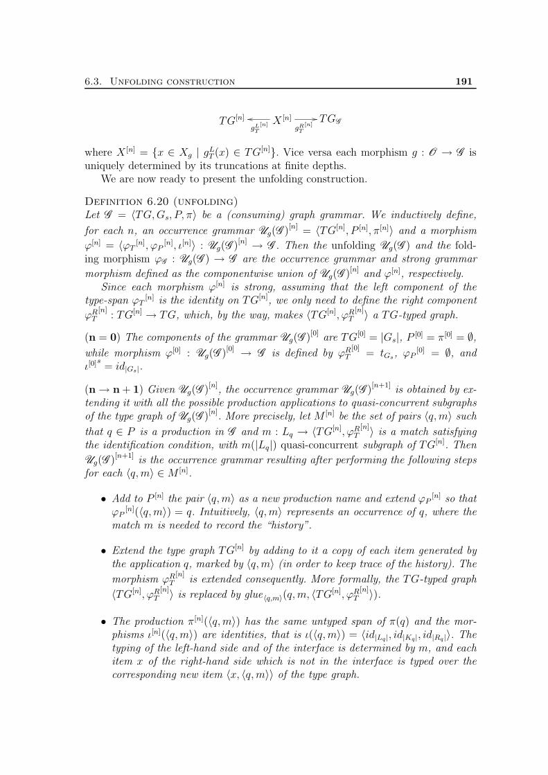
6.3. Unfolding construction 191
TG[n] X [n]
gRT
[n]gLT
[n]TGG
where X [n] = x ∈ Xg | gLT (x) ∈ TG[n]. Vice versa each morphism g : O → G is
uniquely determined by its truncations at finite depths.We are now ready to present the unfolding construction.
Definition 6.20 (unfolding)Let G = 〈TG,Gs, P, π〉 be a (consuming) graph grammar. We inductively define,
for each n, an occurrence grammar Ug(G )[n] = 〈TG[n], P [n], π[n]〉 and a morphism
ϕ[n] = 〈ϕT[n], ϕP
[n], ι[n]〉 : Ug(G )[n] → G . Then the unfolding Ug(G ) and the fold-ing morphism ϕG : Ug(G ) → G are the occurrence grammar and strong grammar
morphism defined as the componentwise union of Ug(G )[n] and ϕ[n], respectively.Since each morphism ϕ[n] is strong, assuming that the left component of the
type-span ϕT[n] is the identity on TG[n], we only need to define the right component
ϕRT[n]
: TG[n] → TG, which, by the way, makes 〈TG[n], ϕRT[n]〉 a TG-typed graph.
(n = 0) The components of the grammar Ug(G )[0] are TG[0] = |Gs|, P[0] = π[0] = ∅,
while morphism ϕ[0] : Ug(G )[0] → G is defined by ϕRT[0]
= tGs, ϕP[0] = ∅, and
ι[0]s
= id|Gs|.
(n→ n + 1) Given Ug(G )[n], the occurrence grammar Ug(G )[n+1] is obtained by ex-tending it with all the possible production applications to quasi-concurrent subgraphsof the type graph of Ug(G )[n]. More precisely, let M [n] be the set of pairs 〈q,m〉 such
that q ∈ P is a production in G and m : Lq → 〈TG[n], ϕRT
[n]〉 is a match satisfying
the identification condition, with m(|Lq|) quasi-concurrent subgraph of TG[n]. Then
Ug(G )[n+1] is the occurrence grammar resulting after performing the following stepsfor each 〈q,m〉 ∈M [n].
• Add to P [n] the pair 〈q,m〉 as a new production name and extend ϕP[n] so that
ϕP[n](〈q,m〉) = q. Intuitively, 〈q,m〉 represents an occurrence of q, where the
match m is needed to record the “history”.
• Extend the type graph TG[n] by adding to it a copy of each item generated bythe application q, marked by 〈q,m〉 (in order to keep trace of the history). The
morphism ϕRT[n]
is extended consequently. More formally, the TG-typed graph
〈TG[n], ϕRT[n]〉 is replaced by glue〈q,m〉(q,m, 〈TG
[n], ϕRT[n]〉).
• The production π[n](〈q,m〉) has the same untyped span of π(q) and the mor-phisms ι[n](〈q,m〉) are identities, that is ι(〈q,m〉) = 〈id|Lq|, id|Kq|, id|Rq|〉. Thetyping of the left-hand side and of the interface is determined by m, and eachitem x of the right-hand side which is not in the interface is typed over thecorresponding new item 〈x, 〈q,m〉〉 of the type graph.

192 Chapter 6. Unfolding and Event Structure Semantics
It is not difficult to verify that for each n, Ug(G )[n] is a (finite depth) nondetermin-
istic occurrence grammar, and Ug(G )[n] ⊆ Ug(G )[n+1], componentwise. ThereforeUg(G ) is a well-defined occurrence grammar. Similarly for each n ∈ N we have
that ϕ[n] is a well-defined morphism from Ug(G )[n] to G , which is the restriction to
Ug(G )[n] of ϕ[n+1]. This induces a unique morphism ϕG : Ug(G )→ G .
The deterministic gluing construction ensures that, at each step, the order inwhich productions are applied does not influence the final result of the step. Moreoverif a production is applied twice at the same match (even if in different steps), thegenerated items are always the same and thus they appear only once in the unfolding.
It is possible to show that the unfolding construction applied to an occurrencegrammar yields a grammar which is isomorphic to the original one. This is essentiallya consequence of the fact that for each production q of an occurrence grammar the(image via the typing morphism of the) left-hand side of q is always quasi-concurrentand the typing morphism tLq satisfies the identification condition, as it can easilyderived from Definition 6.1.
6.4 The unfolding as a universal construction
The unfolding construction has been defined, up to now, only at “object level”. Thissection faces the problem of characterizing the unfolding as a coreflection betweensuitable categories of graph grammars and of occurrence grammars. As in the caseof contextual and inhibitor nets, we first restrict to a full subcategory SW-GGof GG where objects satisfy conditions analogous to those defining semi-weightedP/T Petri nets. Then we show that the unfolding construction can be extended toa functor Ug : SW-GG → O-GG that is right adjoint to the inclusion functorIO : O-GG→ SW-GG.
The restriction to the semi-weighted case is essential for the above categoricalconstruction when one uses general morphisms. However, suitably restricting graphgrammars morphisms to still interesting subclasses (comprising, for instance, themorphisms of [Rib96, HCEL96]) it is possible to regain the categorical semantics forgeneral, possibly non semi-weighted, grammars.
6.4.1 Unfolding of semi-weighted graph grammars
A graph grammar is semi-weighted if the start graph is injective and the right-handside of each production is injective when restricted to produced items (namely, tothe items which are not in the interface). It is possible to show that, if we encode aPetri net N as a grammar GN , according to the translation sketched in Section 5.1.1,then N is a semi-weighted net if and only if GN is a semi-weighted grammar.

6.4. The unfolding as a universal construction 193
Definition 6.21 (semi-weighted grammars)A TG-typed production L ← K → R is called semi-weighted if tR is injective onthe “produced part” of R, namely on |R| − r(|K|). A grammar G is called semi-weighted if the start graph Gs is injectively typed and for any q ∈ P the productionπ(q) is semi-weighted. We denote by SW-GG the full subcategory of GG havingsemi-weighted grammars as objects.
The coreflection result strongly relies on the technical property which is statedin the next lemma. It is important to notice that this is a key point where therestriction to semi-weighted grammars plays a role, since, as we will see, the lemmafails to hold for arbitrary grammars.
Lemma 6.22Let G = 〈TG,Gs, P, π〉 be a semi-weighted grammar, let O = 〈TG′, G′s, P
′, π′〉 be anoccurrence grammar and let f : O → G be a grammar morphism. Then the typespan [fT ] of the morphism is relational.
Proof. Recall from Section 5.3 (Definition 5.32) that the span fT : TG′ ↔ TG is relational if〈fLT , f
RT 〉 : XfT
→ TG× TG′ is mono. In turn, in the categories Set and Graph this amounts tosay
∀x, y ∈ XfT. fRT (x) 6= fRT (y) ∨ fLT (x) 6= fLT (y)
We proceed by contraposition. Consider x, y ∈ XfTsuch that fLT (x) = fLT (y) = z′ and fRT (x) =
fRT (y) = z. Since O is an occurrence grammar, necessarily z′ is in the start graph or in the post-setof some production. Let us assume that z′ ∈Min(O). By definition of grammar morphism, thereexists a morphism k : |Gs| → XfT
such that the following diagram commutes and the square is apullback, where the unlabelled arrow is an inclusion:
Min(O) |Gs|tGs
ιsf
k
TG′ XfTfL
T fRT
TG
The fact that fLT (x) = fLT (y) = z and z ∈ Min(O) implies that there are x′′, y′′ ∈ |Gs| such thatk(x′′) = x and k(y′′) = y. Recalling that the triangle on the right commutes we have
tGs(x′′) = fLT (k(x′′)) = fLT (x) = fLT (y) = fLT (k(y′′)) = tGs
(y′′)
Since the graph Gs is injectively typed, we conclude that x′′ = y′′, and thus x = k(x′′) = k(y′′) = y
that is what we wanted to prove. A similar reasoning applies if the item z belong the post-set ofsome production, since the grammar is semi-weighted and thus productions are injectively typedon the produced part. 2
Observe that, as an immediate consequence of the above lemma, if f : O → G isa grammar morphism, where G is a semi-weighted grammar and O is an occurrencegrammar, then the morphism k, such that fTι
sf , k(Gs, Gs′) (see Definition 5.33,
condition (1)) is uniquely determined. Similarly, for each q ∈ P , with q′ = fP (q),the morphisms kL, kK and kR such that fTι
Xf (q), kX(Xq, Xq′) for X ∈ L,K,R
(see Definition 5.33, condition (2)) are uniquely determined.

194 Chapter 6. Unfolding and Event Structure Semantics
AA′
B′L′
q′1 q′′1
L′′
q′2
LB
q2
q1
B′′
Figure 6.5: The construction mapping safe grammars into i-nets is not functorial.
Some considerations on morphisms between occurrence grammars are now inorder. Let f : O1 → O2 be a grammar morphism, where O1 and O2 are occurrencegrammars. Since, by Lemma 6.22, [fT ] is relational we will sometimes confuse it withthe corresponding relation between the items of TG1 and TG2, namely with
(x1, x2) | ∃x ∈ XfT . fLT (x) = x1 ∧ fRT (x) = x2
and we will write fT (x1, x2) to mean that there exists x ∈ XfT such that fLT (x) = x1
and fRT (x) = x2. By definition of grammar morphism such relation preserves thestart graph and pre-set, post-set and context of productions of O1.
Incidentally, observe that, instead, condition (2.d) in the definition of i-net mor-phism (Definition 4.33) in general does not hold for grammar morphisms. Thereforethe construction, described in Section 6.1, which associates to each safe grammaran inhibitor net is not functorial. An example of occurrence grammar morphism notmeeting the mentioned condition is reported in Figure 6.5. The morphism relatesitems (production names or graph items) of the first grammar to items of the secondgrammar with the same name, (possibly) without “primes”. It is not difficult to seethat this is a legal grammar morphism, but the inhibitor set of q2 is not reflectedsince L ∈ q2, L
′ and L′′ are mapped to L, but q′2 contains only L′′ (while tosatisfy condition (2.d) it should have been q′2 = L′, L′′). The fact that graphgrammar morphisms are more liberal than inhibitor net morphisms is intuitivelyjustified by the particular properties of the inhibitor set of productions in graphgrammars observed in Remark 6.4.
An important property of morphisms between occurrence grammars, which willplay a central role in the proof of the coreflection, is the fact that they “preserve”quasi-concurrency. Furthermore quasi-concurrent items cannot be identified by amorphism. This lemma can be proved along the same lines of an analogous resultwhich hold for morphisms of contextual Petri nets. In fact, the notion of quasi-concurrency disregards the dangling condition, taking into account only causality
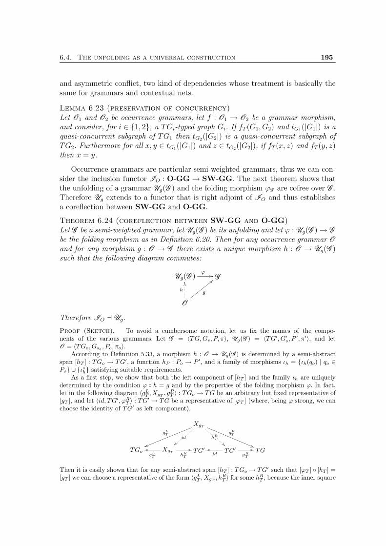
6.4. The unfolding as a universal construction 195
and asymmetric conflict, two kind of dependencies whose treatment is basically thesame for grammars and contextual nets.
Lemma 6.23 (preservation of concurrency)Let O1 and O2 be occurrence grammars, let f : O1 → O2 be a grammar morphism,and consider, for i ∈ 1, 2, a TGi-typed graph Gi. If fT (G1, G2) and tG1(|G1|) is aquasi-concurrent subgraph of TG1 then tG2(|G2|) is a quasi-concurrent subgraph ofTG2. Furthermore for all x, y ∈ tG1(|G1|) and z ∈ tG2(|G2|), if fT (x, z) and fT (y, z)then x = y.
Occurrence grammars are particular semi-weighted grammars, thus we can con-sider the inclusion functor IO : O-GG → SW-GG. The next theorem shows thatthe unfolding of a grammar Ug(G ) and the folding morphism ϕG are cofree over G .Therefore Ug extends to a functor that is right adjoint of IO and thus establishesa coreflection between SW-GG and O-GG.
Theorem 6.24 (coreflection between SW-GG and O-GG)Let G be a semi-weighted grammar, let Ug(G ) be its unfolding and let ϕ : Ug(G )→ Gbe the folding morphism as in Definition 6.20. Then for any occurrence grammar Oand for any morphism g : O → G there exists a unique morphism h : O → Ug(G )such that the following diagram commutes:
Ug(G )ϕ
G
O
h g
Therefore IO ⊣ Ug.
Proof (Sketch). To avoid a cumbersome notation, let us fix the names of the compo-nents of the various grammars. Let G = 〈TG,Gs, P, π〉, Ug(G ) = 〈TG′, G′
s, P′, π′〉, and let
O = 〈TGo, Gso, Po, πo〉.
According to Definition 5.33, a morphism h : O → Ug(G ) is determined by a semi-abstractspan [hT ] : TGo → TG′, a function hP : Po → P ′, and a family of morphisms ιh = ιh(qo) | qo ∈Po ∪ ι
sh satisfying suitable requirements.
As a first step, we show that both the left component of [hT ] and the family ιh are uniquelydetermined by the condition ϕ h = g and by the properties of the folding morphism ϕ. In fact,let in the following diagram 〈gLT , XgT
, gRT 〉 : TGo → TG be an arbitrary but fixed representative of[gT ], and let 〈id, TG′, ϕRT 〉 : TG
′ → TG be a representative of [ϕT ] (where, being ϕ strong, we canchoose the identity of TG′ as left component).
XgT
hRTid
gLT gR
T
TGo XgTgL
T hRT
TG′ TG′id ϕR
T
TG
Then it is easily shown that for any semi-abstract span [hT ] : TGo → TG′ such that [ϕT ] [hT ] =[gT ] we can choose a representative of the form 〈gLT , XgT
, hRT 〉 for some hRT , because the inner square

196 Chapter 6. Unfolding and Event Structure Semantics
becomes a pullback. This shows that, without any loss of generality, we can assume that the leftcomponents of [hT ] and [gT ] coincide.
As far as the family of morphisms ιh is concerned, recall that morphism ιsϕ : |Gs| → |G′s|
is the identity by Definition 6.20; thus, since ϕ h = g implies ιsh ιsϕ = ιsg, we deduce that
ιsh = ιsg. The same holds for the components of ιh(qo) for any production qo ∈ Po, by observingthat ιh(qo) ιϕ(hP (qo)) = ιg(qo) must hold, and that ιϕ(q′) is a triple of identities for each q′ ∈ P ′.
Existence
We will show inductively that for each n ∈ N we can find a morphism h[n] such that the diagram
Ug(G )ϕ
G
O [n]
h[n]
g[n]
commutes, and such that h[n+1] extends h[n]. Then the morphism h we are looking for will be thecomponentwise union of the chain of morphisms h[n]n∈N.
(k = 0) By definition, the occurrence grammar O [0] consists of the start graph of O only, typedidentically on the type graph, with no productions, i.e., O [0] = 〈|Gso
|, ∅, ∅〉. By the considerationsabove, to determine morphism h[0] : O [0] → Ug(G ) we only have to provide the right component
hRT[0]
: XgT
[0] → TG′ of [hT[0]]. Moreover, to be a well defined grammar morphism, h[0] must
preserve the start graph. By condition (1) of Definition 5.33 applied to g[0] : O [0] → G , there
is a morphism k : |Gs| → XgT
[0] such that the diagram below commutes, and the square is apullback. Furthermore, by the pullback properties k is an isomorphism, and, being G a semi-weighted grammar, by Lemma 6.22, k is uniquely determined.
|Gso|
id
|Gs|
tGs
ιsg
k
|Gso| XgT
[0]
gLT
[0]gR
T
[0]TG
Now we define hRT[0]
= tGs k−1, completing the definition of h[0]. The next diagram shows that
h[0] satisfies the requirement of preservation of the start graph. The fact that g[0] = ϕ h[0] easilyfollows by construction.
|Gso|
id
|Gs|tG′
s
ιsg
k
|Gso| XgT
[0]
gLT
[0]hR
T
[0]=tG′
sk−1
TG′
(n → n+1) We have to define morphism h[n+1] : O [n+1] → Ug(G ) by extending h[n] to the itemsof TGo ∪ Po of depth equal to n+ 1. Without any loss of generality we assume that there is justone production qo in O [n+1] with depth(qo) = n + 1 (the general case can be carried out in a
completely analogous way). To ensure ϕP hP[n+1] = gP
[n+1], the production qo must be mappedto a production q′ in Ug(G ), which is an occurrence of the production q = gP (qo) of G . In otherwords, q′ will be 〈q,m〉, with m : Lq → 〈TG′, ϕRT 〉 a match satisfying suitable conditions.

6.4. The unfolding as a universal construction 197
The defining conditions of grammar morphisms, applied to g[n] : O [n] → G , ensure the existenceof a morphism kL, such that the diagram below commutes, where the square is a pullback.
|Lqo|
tLqo
|Lq|tLq
ιLg (qo)
kL
TGo[n] XgT
[n]
gLT
[n]gR
T
[n]TG
Moreover, being G a semi-weighted grammar, by Lemma 6.22 gT is relational and thus the arrowkL is uniquely determined. By Definition 6.18, depth(x) ≤ n for all x ∈ tLqo
(|Lqo|) = •qo ∪ qo,
and thus h[n] is defined on the pre-set and on the context of qo. Therefore we can construct thefollowing diagram.
|Lqo|
tLqo
|Lq|
m=hRT
[n]kL
ιLg (qo)
kL
TGo[n] XgT
[n]
gLT
[n]hR
T
[n]TG′
Notice that m = hRT[n] kL can be seen as a TG-typed graph morphism from Lq to 〈TG′, ϕRT 〉.
In fact, it satisfies ϕRT m = ϕRT hRT
[n] kL = gRT
[n] kL = tLq
. Moreover, recalling that
hT[n] = 〈gLT
[n], hRT
[n]〉, by the diagram above we have that hT
[n](Lqo, 〈|Lq|,m〉). Since by definition
of occurrence grammar tLqo(|Lqo
|) is a quasi-concurrent subgraph of TGo, by using Lemma 6.23,we can conclude that m(|Lq|) is a quasi-concurrent subgraph of TG′. Let us prove that, in addition,the mapping m satisfies the identification condition. First observe that for x, y ∈ |Lq|
m(x) = m(y) ⇒ kL(x) = kL(y). (†)
In fact, assume that m(x) = m(y), let x′ = kL(x) and y′ = kL(y) and suppose x′ 6= y′. From
the fact that m(x) = m(y) we deduce hRT[n]
(x′) = hRT[n]
(y′), and therefore, since h[n] is rela-
tional, gLT[n]
(x′) 6= gLT[n]
(y′). Now observe that, by commutativity of the square in the diagram
above, gLT[n]
(x′), gLT[n]
(y′) ∈ tLqo(|Lqo
|) and moreover hT[n](gLT
[n](x′), z), hT
[n](gLT[n]
(y′), z), wherez = m(x) = m(y). But according to Lemma 6.23 this would imply that tLqo
(|Lqo|) is not quasi-
concurrent, contradicting the definition of occurrence grammar. Hence, as desired, it must bekL(x) = kL(y). We can now conclude that m satisfies the identification condition, namely that forx, y ∈ |Lq|
m(x) = m(y) ⇒ x, y ∈ |Kq|.
In fact, suppose that m(x) = m(y). By (†) above we have that kL(x) = kL(y), hence, by generalpullback properties, ιLg (q0)(x) 6= ιLg (q0)(y) and, by commutativity of the square in the diagram
above, tLqo(ιLg (q0)(x)) = tLqo
(ιLg (q0)(y)). Recalling that tLqosatisfies the identification condition
we get that ιLg (q0)(x) and ιLg (q0)(y) must be in |Kqo|, and thus x, y ∈ |Kq|.
Since m : Lq → 〈TG′, ϕRT 〉 is a match satisfying the identification condition and m(|Lq|)is quasi-concurrent, by definition of unfolding q′ = 〈q,m〉 is a production name in P ′. Then
the production component hP[n+1] of the morphism h[n] can be defined by extending hP
[n] withhP
[n+1](qo) = q′. The diagram above shows that, with this extension, the left-hand side of theproduction is preserved. Now, it can be seen that there is a unique way of extending the type-span

198 Chapter 6. Unfolding and Event Structure Semantics
hT[n] to take into account also the right-hand side of production q′. In fact, consider the diagram
below expressing, for morphism g[n+1], the preservation of the right-hand side of qo.
|Rqo|
tRqo
|Rq|tRq
ιRg (qo)
kR
TGo[n+1] XgT
[n+1]
gLT
[n+1]gR
T
[n+1]TG
To complete the definition of h[n] we must define the right component hRT[n+1]
: XgT
[n+1] → TG′,
extending hRT[n]
on the items which are in X = XgT
[n+1] − XgT
[n]. Now one can verify that kR
establishes an isomorphism between X and |Rq| − rq(|Kq|). Then the condition requiring that
hT[n+1] preserves the right-hand side of qo forces us to define, for each x ∈ X , hRT
[n+1](x) =
tLq′(kR
−1(x)).
The fact that g[n] = ϕ h[n] easily follows by construction.
UniquenessUniqueness essentially follows from the fact that at each step we are forced to define the morphismh as we have done to ensure commutativity. 2
6.4.2 Unfolding of general grammars
A natural question regards the possibility of extending the universal characteriza-tion of the unfolding construction to the whole category GG of graph grammars.It should be noticed that the proof of the uniqueness of the morphism h in Theo-rem 6.24 strongly relies on Lemma 6.22 which in turn requires the grammar G to besemi-weighted. Unfortunately the problem does not reside in our proof technique:the cofreeness of the unfolding of Ug(G ) and of the folding morphism ϕG over Gmay really fail to hold if the grammar G is not semi-weighted.
For instance, consider grammars G1 and G2 in Figure 6.6, where typed graphsare represented by decorating their items with pairs “concrete identity:type”. Thegrammar G2 is not semi-weighted since the start graph is not injectively typed,while G1 is clearly an occurrence grammar. The unfolding Ug(G2) of the grammarG2, according to Definition 6.20, is defined as follows. The start graph and typegraph of Ug(G2) coincide with |Gs2|. Furthermore, Ug(G2) contains two productionsq′2 = 〈q2, m
′〉 and q′′2 = 〈q2, m′′〉, which are two occurrences of q2 corresponding to
the two possible different matches m′, m′′ : Lq2 → Gs2 (the identity and the swap).Observe that there exists a morphism g : G1 → G2 which is not relational, i.e., the
property in Lemma 6.22 fails to hold. The component gP on productions is defined bygP (q1) = q2, while the type span gT is defined as follows: XgT is a discrete graph withtwo nodes x and y, gLT (x) = gLT (y) = A and gLT (x) = gLT (y) = B (see the bottom rowof the diagram in Figure 6.6). Consider the pullback-retyping diagram in Figure 6.6,expressing the preservation of the start graph for morphism g (condition (1) ofDefinition 5.33). Notice that there are two possible different morphisms k and k′

6.4. The unfolding as a universal construction 199
|Gin2 ||Gin1 |
Grammar G 1 Grammar G 2
q1
1
x
TG1 XgTTG2
B
q2
A
1 2
y
A 2:BB1:A 1:BTG1 = Gin2 =TG2 =Gin1 =
2:B1:A 1:B
Figure 6.6: The grammars G1 and G2, and the pullback-retyping diagram for theirstart graphs.
from |Gs2| to XgT (represented via plain and dotted arrows, respectively) makingthe diagram commutes and the square a pullback. Now, it is not difficult to seethat, correspondingly, we can construct two different morphisms hi : G1 → Ug(G2)(i ∈ 1, 2), such that ϕG2 hi = g, the first one mapping production q1 into q′2 andthe second one mapping q1 into q′′2 . An immediate consequence of this fact is theimpossibility of extending Ug on morphisms, in order to obtain a functor which isright adjoint to the inclusion I : O-GG→ GG.
The above considerations, besides giving a negative result, also suggest a wayto overcome the problem. An inspection of the proof of Theorem 6.24 reveals thatthe only difficulty which prevents us to extend the result is the non uniqueness ofthe morphisms k, kL, kK and kR in the pullback-retyping constructions. In otherwords, if we consider any morphism g : O → G such that [gT ] is relational then wecan prove, as in Theorem 6.24, the existence of a unique morphism h : O → Ug(G )making the following diagram commute:
Ug(G )ϕ
G
O
hg
Hence the coreflection result can be regained by limiting our attention to a (non
full) subcategory GG of GG, where objects are general graph grammars, but allmorphisms have a relational span as type component. Then, the only thing to proveis that the unique morphism h constructed in the proof of Theorem 6.24 is indeedan arrow in GG.

200 Chapter 6. Unfolding and Event Structure Semantics
The naıve solution of taking all relational morphisms as arrows of GG does notwork because they are not closed under composition. A possible appropriate choiceis instead given by the category GGR, where the arrows are grammar morphisms fsuch that the left component fLT of the type span is mono.
Definition 6.25 (Category GGR)We denote by GGR the lluf subcategory of GG, where for any arrow f the left
component fLT of the type span is mono. Furthermore we denote by O-GGR the fullsubcategory of GGR having occurrence grammars as objects.
By the properties of pullbacks, the arrows in GGR are closed under compositionand thus GGR is a well-defined subcategory of GG.
Theorem 6.26 (unfolding as coreflection - reprise)The unfolding construction can be turned into a functor U R
g : GGR → O-GGR,
having the inclusion I RO : O-GGR → GGR as left adjoint, establishing a coreflec-
tion between the two categories.
Proof. By the considerations above, the only thing to prove is that the morphism h constructedas in the proof of Theorem 6.24 is an arrow in O-GGR. But this is obvious since, by constructionhLT = gLT and thus hLT is mono. 2
Alternatively, the result can be proved for the subcategory GGL of GG wherearrows are grammar morphisms having the right component of the type span whichis mono. Clearly this is a well defined subcategory, while proving that the morphismconstructed in the proof of Theorem 6.24 is an arrow in O-GGL requires someadditional effort.
Observe that although not completely general, the above results regard a re-markable class of grammar morphisms. In particular they comprise the morphismsadopted in [HCEL96, Rib96] where the type component of an arrow from G1 to G2
is a partial graph morphism from TG1 to TG2, and from TG2 to TG1, respectively.Finally, it is worth remarking that strong grammar morphisms are arrows in
GGR, a fact that, in the next chapter, will allow us to fruitfully use Theorem 6.26to establish a relation between the unfolding and the deterministic process semanticsof a grammar (see Section 7.4).
6.5 From occurrence grammars to event struc-
tures
Starting from the semantics of graph grammars given in terms of occurrence gram-mars, the aim of this section is to provide a more abstract semantics based on(suitable kind of) event structures and domains, following the guidelines traced inthe First Part for contextual and inhibitor nets. Due to the similarity betweengrammars and inhibitor nets, it comes as no surprise that inhibitor event structures,

6.5. From occurrence grammars to event structures 201
the generalization of Winskel’s event structures introduced in Chapter 4, are ex-pressive enough to encode the causal structure of grammar computations. The iesassociated to an occurrence grammar is obtained by forgetting the state, and remem-bering the productions of the grammar and the relationship among them. Recallingthe encoding of safe grammars into i-nets, the formal definition is a straightforwardgeneralization of the construction taking an occurrence i-net into the correspondingies. By using the results in Chapter 4 the ies semantics can be finally “translated”into a domain and pes semantics.
The configurations of the ies associated to an occurrence grammar O can beshown to coincide with the configurations of the grammar O , as defined in Sec-tion 6.1. Furthermore the extension ordering on the configurations of such ies canbe characterized by using only the relations of causality and asymmetric conflictdefined directly on the grammar, thus providing a simpler characterization of thedomain semantics.
6.5.1 An IES semantics for graph grammars
We next introduce the DE-relation naturally associated to an occurrence grammarO , which is is used to define first a pre-ies and then an ies for the grammar O .
Definition 6.27 (pre-ies for an occurrence grammar)Let O = 〈TG, P, π〉 be an occurrence grammar. The pre-ies associated to O is definedas IpO = 〈P, p
O〉, with O ⊆ 2P1 ×P ×2P , given by: for q, q′ ∈ P and x ∈ Items(TG)
• if q• ∩ ( •q′ ∪ q′) 6= ∅ then pO(∅, q′, q)
• if ( •q ∪ q) ∩ •q′ 6= ∅ then pO(q′, q, ∅);
• if x ∈ q (and thus x is an edge in the type graph TG) then pO( •s, q, s•).
As for inhibitor nets, IpO is a pre-ies satisfying also condition (1) of the definitionof ies. Therefore, as discussed in Proposition 4.5, it can be “saturated” in order toobtain an ies.
Definition 6.28 (ies for an occurrence grammar)The ies associated to an occurrence grammar O, denoted by IO = 〈P, O〉, is defined
as IpO .
Recall that the causality, asymmetric conflict and conflict relations of IO and IpOcoincide. They will be denoted by <i
O , րiO and #i
O , respectively. The superscript“i” is used to distinguish these relations from the relations <O and րO , associateddirectly to the occurrence grammar in Section 6.1.
We now prove that the construction which maps an occurrence grammar intothe corresponding ies IO can be turn into a functor. This is not completely obvious,since, as observed in Section 6.4, grammar morphisms are more liberal than i-net

202 Chapter 6. Unfolding and Event Structure Semantics
morphisms because, in general, they do not reflect the inhibitor set of productions.In the proof we will exploit the fact that, as explained in Section 6.4, the typecomponent of a morphism between occurrence grammars can be thought of as arelation, preserving the start graph as well as the pre-set, post-set and context ofproductions.
Proposition 6.29Let O0 and O1 be occurrence grammars and let h : O0 → O1 be a grammar morphism.Then hP : IO0 → IO1 is an ies morphism.
Proof (Sketch). For k ∈ 0, 1, let <k, րk and #k be the relations of causality, asymmetricconflict and conflict in the pre-ies Ipk = 〈Pk,
pk〉 associated to the grammar Ok. As in the case of
i-nets, we show that hP : Ip0 → Ip1 satisfies conditions (1)-(4) in the hypotheses of Lemma 4.9 and
thus that hP is an ies morphism between the corresponding “saturated” ies’s.
Relying on the analogy between occurrence grammar and i-nets morphisms, most of the prop-erties can be proved exactly as for i-nets. We will treat explicitly only only some cases whichinvolve the inhibitor set of productions, since, as observed before, grammar morphisms impose onthe inhibitor set of productions requirements which are weaker than those of i-nets morphisms.
1. hP (q0) = hP (q′0) ∧ q0 6= q′0 ⇒ q0#0q′0.
Treated as for i-nets.
2. p1(∅, hP (q0), A1) ⇒ ∃A0 ⊆ h
−1P (A1). A0 <0 q0.
Let us assume p1(∅, hP (q0), A1). By definition of p
1 one of the following holds:
(a) A1 = q1 and q1• ∩ •h(q0) 6= ∅
(b) A1 = q1 and q1• ∩ h(q′0) 6= ∅
(c) ∃x1 ∈ h(q0).•x1 = ∅ ∧ x1
• = A1,
The first two cases are treated as for i-nets. In case (c), observe that x1 is necessarily anedge in the start graph of O1, with source or target in a node n1 which must be in thestart graph of O1 as well. By the properties of occurrence grammar morphisms, there are aunique node n0 and a unique edge x0 such that hT (n0, n1) and hT (x0, x1). Then n0 ∈ •q0,x0
• <0 t0 and x0• ⊆ h−1
P (A1).
3. p1(hP (q′0), hP (q0), ∅) ⇒ q0 ր0 q
′0.
Treated as for i-nets.
4. p1(hP (q′0), hP (q0), A1) ∧A1 6= ∅ ⇒ ∃a0 ⊆ q′0. ∃A0 ⊆ h
−1P (A1). 0(a0, q0, A0).
Assume p1(hP (q′0), hP (q0), A1) and A1 6= ∅. Thus, by definition of p
1 there must bean edge x1 ∈ hP (q0) ∩ hP (q′0)
• such that A1 = •x1. The figure below gives a graphicalrepresentation of the situation, in which the set of productions A1 is depicted as a singlebox.

6.5. From occurrence grammars to event structures 203
h(q′0)
h(q0)
x1n1
A1
By properties of occurrence grammar morphisms, we can find in the post-set of q′0 an edgex0 with source or target in the node n0, and in the pre-set of q0 a node n′
0 such that thetype component hT relates n0 and n′
0 to n1, while x0 is related to x1.
x0n0
n′0
q′0
q0
A0
Now, two possibilities arise: if n0 = n′0 then we immediately conclude that p
0(q′0, q0, x0
•)and clearly x0
• ⊆ h−1P (A1).
If instead n0 6= n′0, first observe that n0 and n′
0 are not in the start graph. In fact, supposethat n0 is in the start graph. Then, by definition of grammar morphism, also n1 is in thestart graph and therefore one can easily conclude that also n′
0 is in the start graph. Hencen0, n
′0 is quasi concurrent, but hT (n0, n1) and hT (n′
0, n1), which is a contradiction byLemma 6.23.
Now, considering q′′0 ∈•n0 and q′′′0 ∈
•n′0, we have q′′0 #0q
′′′0 . Since q′0 produces the edge
x0, necessarily n0 ∈ q′0• ∪ q′0 and therefore q′′0 ≤0 q
′0. Furthermore, q′′′0 ≤0 q0 and therefore
q0#0q′0, which implies q0 ր0 q
′0. Recalling how a pre-ies is saturated to give rise to an ies
(see Proposition 4.5) we finally conclude 0(q′0, q0, ∅). 2
By the above proposition the functor which maps each occurrence grammar tothe corresponding ies defined as in Definition 6.28 and each grammar morphism toits production component is well-defined.
204 Chapter 6. Unfolding and Event Structure Semantics
Definition 6.30 (from occurrence grammars to ies’s)Let Eg : O-GG→ IES be the functor defined as:
• Eg(O) = IO , for each occurrence grammar O;
• Eg(h : O0 → O1) = hP , for each morphism h : O0 → O1.
Now, by using the functor Li : IES → Dom defined in Chapter 4, mappingeach ies into its domain of configurations we can obtain a domain and then a pessemantics for grammars.
6.5.2 A simpler characterization of the domain semantics
In Section 6.1 we have introduced the configurations of nondeterministic occurrencegrammars as a mean to capture the possible deterministic computations of suchgrammars. We next show that they coincide with the configurations of the associ-ated inhibitor event structure, thus allowing for a simpler characterization of thecorresponding domain.
We first observe a property of the ies associated to an occurrence grammar, whichgeneralizes the observation in Remark 6.4. Recall that in general ies’s when, forinstance, (q′, q, q′′), if the three events q, q′, q′′ appear in the same computationthen there are two possible orders of execution, namely q; q′; q′′ and q′; q′′; q. Instead,in the case of occurrence grammars O , if O(q′, q, q′′) then by definition of O ,q′• ∩ q 6= ∅. Therefore, as observed in Remark 6.4, necessarily q′ must precede q,i.e., q′ ր q, since q′ produces or preserves a node which is consumed by q. Hence,in this case, the only possible order of execution is q′; q′′; q. As a consequence, foreach configuration C the associated choice relation →C is uniquely determined bythe events of the configuration and coincides with the asymmetric conflict.
Proposition 6.31Let O = 〈TG, P, π〉 be an occurrence grammar and let Ei(O) = 〈P, O〉 be thecorresponding ies. Then
• O(q′, q, A) ⇒ q′ րi q ∧ ∀q′′ ∈ A. q′′ րi q;
• 〈C, →〉 ∈ Conf (I) ⇒ → =րiC.
It is easy to realize that the relations <O andրO , which do not take into accountthe dependencies induced by the dangling condition, are included in the correspond-ing relations <i
O andրiO . The above proposition entails that the transitive closures
of the two asymmetric conflict relations coincide, namely
(րO)∗ = (րiO)∗
and thus, when restricted to a configuration, they express essentially the same prece-dences. This observation allows one to prove that the configurations of an occur-rence grammar are exactly the configurations of the associated ies. Furthermore

6.5. From occurrence grammars to event structures 205
the extension order on the ies’s configurations can be characterized by using onlythe asymmetric conflict relation րO associated to the grammar. Besides providinga simpler characterization of the domain semantics of a grammar, this result en-forces our confidence in the appropriateness of the ies associated to an occurrencegrammar, since, as we already observed, the configurations of an occurrence gram-mar correctly represents all the different possible deterministic computations of thegrammar.
Proposition 6.32 (domain for an occurrence grammar)Let O be an occurrence grammar and let Eg(O) be the corresponding ies. ThenC ∈ Conf (O) iff C ∈ Eg(O). Moreover the order relation over the prime algebraicdomain Li(Eg(O)) can be characterized as
C ⊑ C ′ iff C ⊆ C ′ and ∀q ∈ C. ∀q′ ∈ C ′. q′ րO q ⇒ q′ ∈ C.
Notice that, formally, the order on configuration is the same as for contextual nets: aconfiguration C cannot be extended with a production inhibited by some of the pro-ductions already present in C. However recall from Definition 6.9, that the asymmet-ric conflict by itself, without any additional information on the dangling condition,is not sufficient to define which subsets of events are configurations.
Hereafter we will always use the above characterization of the domain semanticsof a grammar. Consequently we will never refer to the asymmetric conflict, conflictand causality relations of the ies IO , using instead the relations defined directly onthe grammar O .
Recall that the pes associated to the domain Li(Eg(O)), namely P(Li(Eg(O)))),consists of the set of prime elements of the domain (with the induced partial orderas causality and the inconsistency relation as conflict), i.e., the unique (up to iso-morphisms) pes having Li(Eg(O)) as domain of configurations.
As already seen for contextual and inhibitor nets, there is not a one to one corre-spondence between events of P(Li(Eg(O))) and productions in O : a different eventis generated for any possible “history” of each production in O . This phenomenonof “duplication of events” is related to the fact that the pes represents the depen-dencies arising between productions in graph grammar computations by means ofcausality and symmetric conflict. A situation of asymmetric conflict like q1 ր q2 ingrammar G1 of Figure 6.1, is encoded in the pes by the insertion of a single evente1 corresponding to q1, and two “copies” e′2 ad e′′2 of q2, the first one in conflict withe1 and the second one caused by e1 (see Figure 6.7.(a)). For what concerns the dan-gling condition, consider the grammar G2 in Figure 6.1. In this case three conflictingevents are generated corresponding to q4: e4 representing the execution of q4 fromthe start graph, which inhibits all other productions, and e′4, e
′′4 representing the
execution of q4 after q2 and q3, respectively.

206 Chapter 6. Unfolding and Event Structure Semantics
e′2 # e1
≤
e′′2
e1≤ ≤
# e4
e2
≤
# e3
≤
e′4 e′′4
Figure 6.7: Encoding asymmetric conflict and dangling condition in prime eventstructures.
6.6 A related approach: unfolding semantics of
SPO graph grammars
An unfolding construction for graph grammars in the single-pushout (spo) approachhas been proposed by Ribeiro in her doctoral thesis [Rib96]. She defines an unfoldingfunctor from a category of spo graph grammars to a category of (abstract) occur-rence grammars, showing that it is a right adjoint to a suitable folding functor .In this section we discuss the relation between the construction introduced in thischapter and the one in [Rib96]. Although the two constructions rely on similar basicideas, concretely, the differences between the two settings makes hard a formal directcomparison. Therefore we will mainly try to point out some conceptual differencesand analogies.
First of all in the spo approach there are no application conditions. Withoutgetting into technical details, if a production specifies both the preservation and thedeletion of an item, then such an item is removed by the application of the produc-tion. Furthermore, an edge which should remain dangling after the application of aproduction because its source (or target) node is deleted, is automatically deleted aswell. For the presence of these “side-effects” the pre-set of a production, intended asthe set of items which are “consumed” by the production, depends also on the con-sidered match, and the application of a production may remove items which are notmentioned explicitly in the production itself. Consequently, the notion of causalityfor spo graph grammars is less intuitive if compared with the dpo case, and thecorrespondence between the theory of spo grammars and the theory of Petri netsbecomes looser. For instance, if a production q1 produces and edge e, and q2 deletese as side effect, we may wonder whether q2 should causally depend on q1 or not. Ifwe assume that causality is induced by the flow of data in the system, the answershould be that q1 ≤ q2 since q2 consumes something which is produces by q1. Onthe other hand, the application of q1 is not necessary to make q2 applicable, sinceq2 does not explicitly require the presence of resources generated by q1. Thus, ifq1 ≤ q2 means that the application of q1 precedes q2 in each computation where q2

6.6. Unfolding of SPO graph grammars 207
is applied, then there should be no causal relationship between q1 and q2.Although the above question is not completely trivial, the more reasonable choice
seems the latter. In this case, the notions of causality and of asymmetric conflict(called weak conflict in [Rib96]) can be defined disregarding the mentioned side-effects. This is basically due to the fact that when a production uses (consumesor preserves) an edge, it must use necessarily the corresponding source and targetnodes, and therefore dependencies related to side-effects can be detected by lookingonly at explicitly used items.
A relevant difference with our work resides in the notion of occurrence grammars.The thesis [Rib96] introduces the so-called doubly typed occurrence grammars, wherethe type graph is itself typed over another graph of types. Intuitively, a doubly typedoccurrence grammar is a sort of process where only the “type component” of theprocess morphism is specified. This essentially means that each production of such agrammar can be thought of as an instance of a production of another grammar, forwhich the match is already specified. Because of the double typing, the category ofoccurrence grammars considered in [Rib96] is not a subcategory of the category ofgraph grammars, and the left adjoint of the unfolding functor is not the inclusion,but a folding functor which basically forgets the intermediate typing.
The grammar which is obtained from a doubly-typed occurrence grammar byforgetting the intermediate typing satisfies conditions which are similar to thoseimposed on our occurrence grammars. However, again the theory necessarily divergesbecause of the absence of the application condition in the spo approach. When asingle rule requires both the preservation and the deletion of an item, accordingto our definition it should be in asymmetric conflict with itself, and thus neverapplicable. As mentioned above, instead in the spo approach such kind of rule canbe applied and the “conflictual requirement” is resolved in favor of deletion.
The final difference which must be taken into account regards the kind of mor-phisms on graph grammars. In [Rib96] the type component of a morphism from agrammar G1 to G2 is a partial function from TG2 to TG1. Since such partial functioncan be seen as a span where the right component is injective, in this respect themorphisms of [Rib96] are less general than ours. On the other hand, to character-ize the parallel composition of graph grammars as a categorical limit, the imageunder a morphism of a production in G1 is required only to be a sub-productionof the corresponding production in G2. When moving to occurrence grammars, alsothe morphisms of [Rib96] must preserve the components of a production. Howeverpreservation is required only up to isomorphism and this seems the reason why, ata first glance, the unfolding cannot be turned into a functor. The problem is solvedby considering a category of abstract occurrence grammars, where objects are iso-morphisms classes of grammars. Then the unfolding can be expressed as a functorwhich establishes an adjunction between the category of graph grammars and suchcategory of abstract occurrence grammars.
Summing up, many analogies exist between the two constructions, but the subtledifferences deeply connected with the diversity of the spo and dpo approaches,

208 Chapter 6. Unfolding and Event Structure Semantics
makes us skeptical about the possibility of establishing a formal link between thetwo results. A possibility still not explored could be to resort to the formulationof the dpo approach in term of spo approach (with application conditions) to seeif a common theory can be developed, although in the past such an approach hasrevealed some limits.

Chapter 7
Concatenable Graph Processes
This chapter introduces a semantics for dpo graph grammars based on concaten-able graph processes. Conceptually, concatenable graph processes are very close toderivation traces in that they are aimed at representing the deterministic (trulyconcurrent) computations of a grammar. However, differently from traces they pro-vide an explicit characterization of the events occurring in computations and of thedependency relationships among them.
Relying on the theory developed in the previous chapter, first a deterministicgraph process is naturally defined as a special graph process such that the whole setof productions of the underlying occurrence grammar is a configuration, and thusall the productions of the process can be applied in a single computation. Given adeterministic process ϕ : O → G , the morphism ϕ can be used to map derivationsin the underlying occurrence grammar O to corresponding derivations in G . Thebasic property of a graph process is that the derivations in G which are in the rangeof such mapping constitute a full class of shift-equivalent derivations. Therefore theprocess can be regarded as an abstract representation of such a class and plays a rolesimilar to a canonical derivation [Kre77]. Although obtained by following a differentpath, the above notion of deterministic process can be seen easily to coincide withthe previous proposals in [CMR96, BCM98a].
Graph processes are not naturally endowed with a notion of sequential compo-sition, essentially because of the same problem described for abstract derivations: ifthe target graph of a process is isomorphic to the source graph of a second process,the naıve idea of composing the two processes by gluing the two graphs accordingto an isomorphism does not work. In fact, in general we can find several distinctisomorphisms relating two graphs, which may induce sequential compositions of thetwo processes which substantially differ from the point of view of causality. Using thesame technique adopted for derivations, concatenable graph processes are defined asgraph processes enriched with the additional information (a decoration of the sourceand target graphs) needed to concatenate them.
Then the claim that deterministic processes and derivation traces give conceptu-ally equivalent descriptions of the system is formalized by showing that the category

210 Chapter 7. Concatenable Graph Processes
Tr[G ] of concatenable (parallel) derivation traces (Definition 5.27) is isomorphic tothe category of concatenable (abstract) processes CP[G ].
Finally, we show that the unfolding and the deterministic process semantics canbe reconciled by following the approach described in the Introduction. As alreadydone for generalized nets, we prove that the domain associated to a grammar viathe unfolding construction can be characterized as the collection of deterministicprocesses starting from the initial graph, endowed with a kind of prefix order.
The rest of the chapter is structured as follows. Section 7.1 introduces determin-istic graph processes as special nondeterministic processes, giving evidence of theirrelation with the previous notions in the literature. Section 7.2 presents the cate-gory CP[G ] of concatenable processes for a grammar G . The equivalence betweenthe concatenable trace semantics (introduced in Section 5.2) and the concatenableprocess semantics is proved in Section 7.3. Finally, Section 7.4 provides a connectionbetween the unfolding and the deterministic process semantics of a grammar.
7.1 Deterministic graph processes
A nondeterministic graph process (Definition 6.13) represents a class of derivationsof a grammar G by means of a nondeterministic occurrence grammar O . A (specialkind of) grammar morphism from O to the given grammar G allows one to mapcomputations in O to computations in G .
To obtain a deterministic graph process, namely an appropriate representativeof a single concurrent computation in G we must restrict our attention to occur-rence grammars where all productions can be applied in a single computation. ByProposition 6.11 we know that this is the case when the whole set of productions ofO is a configuration of O itself.
Definition 7.1 (deterministic occurrence grammar)An occurrence grammar O = 〈TG, P, π〉 is called deterministic if the set P of itsproductions is a configuration of O. For a deterministic occurrence grammar O wedenote by Max(O) the set of items of the type graph TG which are maximal withrespect to causality.
Recalling the notion of configuration of an occurrence grammar (Definition 6.9),we see that an occurrence grammar is deterministic if the transitive closure of theasymmetric conflict relation is a finitary partial order. Furthermore whenever aproduction consumes a node in the type graph, then productions removing theedges with source or target in that node must be present as well. Observe that thefirst condition implies the absence of forward conflicts, namely each item of the typegraph can be consumed by at most one production, i.e., |x•| ≤ 1 for each item xof the type graph (while in general general occurrence grammars only backwardconflicts are forbidden).

7.1. Deterministic graph processes 211
In the case of finite grammars the above conditions can be expressed in a simplerway. Since there are only finitely many productions, the first condition amountsto the acyclicity of asymmetric conflict. Assuming the first condition, and thusthe absence of forward conflicts, the second condition can be expressed by simplyrequiring Max(O) to be a well-defined graph.
Proposition 7.2 (finite deterministic occurrence grammar)A finite occurrence grammar O is deterministic iff
1. րO is acyclic;
2. Max(O) is a well-defined subgraph of the type graph.
Proof. Let O be an occurrence grammar satisfying (1) and (2) above. We must show that its setof productions P is a configuration of O. The fact that (րO)∗ is a finitary partial order immediatelyfollows from the acyclicity of րO and the fact that P is finite. Trivially P is closed with respectto causality. It remains to prove the last condition in the definition of configuration, namely thatgiven any edge e ∈ TG, if e ∩ P 6= ∅ and •e ⊆ P then e• ∩ P 6= ∅. Suppose that q ∈ e ∩ P forsome edge e (clearly •e ⊆ P since P contains all productions of O). Hence there is a node n ∈ •q
which is the source or target of e. Therefore n ≤ q and thus n 6∈ Max(O). Since Max(O) is awell-defined graph, necessarily e 6∈Max(O) and thus there must exist q′ ∈ P such that e ∈ •q′, orequivalently q′ ∈ e•.
The converse implication is proved in an analogous way. 2
The above proposition, besides giving an alternative simpler characterization ofdeterministic occurrence grammars, shows that they coincide with the occurrencegrammars of [CMR96, BCM98a, BCE+99]. It is worth remarking that in such papers,which are concerned only with deterministic computations, the causality relation isused to represent the order of execution within the specific concurrent computation,and as such it plays the role which is played here by the transitive closure of theasymmetric conflict relation. We apologize if the reader may get a bit confused bythis change in terminology, but we hope she will agree that in this general contextthe terminology we adopted is more appropriate.
Let O be a deterministic occurrence grammar. Recall that, by Proposition 6.11,for any finite configuration C of O , there is a derivation Min(O) ⇒∗C reach(C)applying all the productions of C in any order compatible with the asymmetricconflict. In particular, if the grammar is finite, we can take as C the full set P ofproductions of O . It is easy to verify that reach(P ) = Max(O) and therefore
Min(O)⇒∗P Max(O)
using all productions in P exactly once, in any order consistent with րO .This helps in understanding why a deterministic graph process of a grammar
G , that we are going to define simply as a graph process having a deterministicunderlying occurrence grammar, can be seen as representative of a set of derivationsof G where independent steps may be switched.
Observe that a deterministic occurrence grammar is a fully fledged graph gram-mar and thus one may “execute” it by considering any possible derivation beginning

212 Chapter 7. Concatenable Graph Processes
5:S
4:C
3: req4:C
6:S
4:C
6:busy
SER' :
6:S
4:C
6:S
4:C
6:busy
6:S
4:C
REL' :
4:C
2: job4:C 4:C
4: job
5:req
REQ'2 :4:C
0: job4:C 4:C
2: job
3:req
REQ'1 :
6:S
4:C
6:busy
4: job
5: req
5:S
2: job
3: req
0: jobTGp
Figure 7.1: A graph process of the grammar C -S .
from the start graph Min(O). However, the discussion above stresses that, if we areinterested in using a deterministic occurrence grammar to represent a deterministiccomputation, it is natural to consider only those derivations which are consistentwith the asymmetric conflict.
Definition 7.3 (deterministic graph process)Let G be a graph grammar. A graph process ϕ : Oϕ → G of G is called (finite)deterministic if the the occurrence grammar Oϕ is (finite) deterministic.
As for general nondeterministic processes, we can assume that the left component ofthe type span ϕT is the identity; furthermore to simplify the notation we will simplywrite ϕT to denote the right component ϕRT of the type span. We will denote byMin(ϕ) and Max(ϕ) the subgraphs Min(Oϕ) and Max(Oϕ) of TGϕ. Moreover, byanalogy with the case of nets, the graphs Min(Oϕ) and Max(Oϕ) typed over TGG
by (the suitable restrictions of) ϕT will be denoted by •ϕ and ϕ• respectively, andcalled the source and target graphs of the process.
Example 7.4 (deterministic process)Figure 7.1 shows a deterministic process for grammar C -S of Example 5.9. Thetyping morphisms from the productions of the process to TGϕ are inclusions, andthe start graph is the subgraph of TGϕ containing the items 5 : S, 0 : job and 4 : C(thus exactly the start graph G0 of C -S ), because these are the only items whichare not generated by any production.
The morphism ϕT : TGϕ → TG is represented, as usual, by labelling the itemsof TGϕ with their image in TG, and the mapping ϕP from the productions of theprocess to those of C -S is the obvious one. 2

7.2. Concatenable graph processes 213
7.2 Concatenable graph processes
Since deterministic processes represent (concurrent) computations and express ex-plicitly the dependencies between single rewriting steps, it is very natural to requirea notion of processes composition “consistent” with such dependencies. To definesuch notion we have to face the same problem described for traces, namely giventwo processes ϕ1 and ϕ2 such that ϕ1
• ≃ •ϕ2, the naıve idea of composing the twoprocesses by gluing the target of ϕ1 with the source of ϕ2 does not work, since theremight be several different isomorphisms between the graphs ϕ1
• and •ϕ2, which maylead to different results. The problem is solved as for traces, by decorating the source•ϕ and the target ϕ• of each process ϕ. A concatenable graph process is defined as agraph process equipped with two isomorphisms relating its source and target graphsto the corresponding canonical graphs. The two isomorphisms allow us to define adeterministic operation of sequential composition of processes consistent with causaldependencies, which is then exploited to define a category CP[G ] having abstractgraphs as objects and (abstract) concatenable processes as arrows. Clearly the no-tion of sequential composition is meaningful only for unmarked processes whosesource is a generic graph (see Definition 6.15).
Definition 7.5 (concatenable graph process)Let G = 〈TG,Gs, P, π〉 be a typed graph grammar. A concatenable graph process forG is a triple
γ = 〈m,ϕ,M〉
where ϕ is an unmarked deterministic process of G and m : Can(•ϕ) → •ϕ, M :Can(ϕ•)→ ϕ• are isomorphisms (of TG-typed graphs).
It should be noted that the two isomorphisms to the source and target graphsof a process play the same role of the ordering on minimal and maximal placesof concatenable processes in Petri net theory [DMM96]. From this point of view,concatenable graph processes are related to deterministic graph processes in thesame way as the concatenable processes of [DMM96] are related to the classicalGoltz-Reisig processes for P/T nets [GR83].
The notion of isomorphism between concatenable processes is the natural gen-eralization of that of graph process isomorphism (see Proposition 6.14). In this casethe mapping between the type graphs of the two processes is also required to be“consistent” with the decorations.
Definition 7.6 (isomorphism of concatenable processes)Let γ1 = 〈m1, ϕ1,M1〉 and γ2 = 〈m2, ϕ2,M2〉 be two concatenable processes of agrammar G . An isomorphism between γ1 and γ2 is an isomorphism of processes

214 Chapter 7. Concatenable Graph Processes
〈fT , fP 〉 : ϕ1 → ϕ2 such that the following diagrams commute:
•ϕ1
fT
Can(•ϕ1)‖
Can(•ϕ2)
m1
m2 •ϕ2
ϕ1•
fT
Can(ϕ1•)
‖Can(ϕ2
•)
M1
M2ϕ2•
where fT : •ϕ1 →•ϕ2 and fT : ϕ1
• → ϕ2• denote the restrictions of fT to the
corresponding graphs. If there exists an isomorphism f : γ1 → γ2 we say that γ1 andγ2 are isomorphic and we write γ1
∼= γ2.
Definition 7.7 (abstract concatenable process)An abstract concatenable process is an isomorphism class of concatenable processes.It is denoted by [γ], where γ is a member of that class.
As usual, a particular role is played by processes based on grammars with emptyset of productions.
Definition 7.8 (discrete process)A discrete concatenable process is a concatenable process γ = 〈m,ϕ,M〉 suchthat the corresponding occurrence grammar Oϕ has an empty set of productions.In this case •ϕ = ϕ• = 〈TGϕ, ϕT 〉 and the concatenable process is denoted bySymG (m,G,M), where G = •ϕ = ϕ•.
Notice that two discrete concatenable processes SymG (mj , Gj,Mj) (j ∈ 1, 2)of a grammar G are isomorphic if and only if m−1
1 M1 = m−12 M2. Therefore, an
abstract discrete concatenable process [SymG (m,G,M)] can be characterized as:
SymG (m′, G′,M ′) | G ≃ G′ ∧ m′−1 M ′ = m−1 M.
The isomorphism m−1 M is called the automorphism on Can(G) induced by the(abstract) discrete concatenable process.
Given two concatenable processes γ1 and γ2 such that the target graph of the firstone and the source graph of the second one, as well as the corresponding decorations,coincide, we can concatenate them by gluing the type graphs along the common part.
Definition 7.9 (sequential composition)Let G = 〈TG,Gs, P, π〉 be a typed graph grammar and let γ1 = 〈m1, ϕ1,M1〉 andγ2 = 〈m2, ϕ2,M2〉 be two concatenable processes for G , such that ϕ1
• = •ϕ2 andM1 = m2. Suppose moreover that the type graphs of γ1 and γ2 overlap only onMax(ϕ1) = Min(ϕ2) and suppose also Pϕ1 and Pϕ2 disjoint. Then the concretesequential composition of γ1 and γ2, denoted by γ1 ; γ2, is defined as
γ = 〈m1, ϕ,M2〉,

7.2. Concatenable graph processes 215
where ϕ is the (componentwise) union of the processes ϕ1 and ϕ2. More preciselythe type graph TGϕ is
TGϕ = 〈NTGϕ1∪NTGϕ2
, ETGϕ1∪ETGϕ2
, s1 ∪ s2, t1 ∪ t2〉,
where si and ti are the source and target functions of the graph TGϕi for i ∈ 1, 2,and analogously the typing morphism ϕT = ϕ1T ∪ ϕ2T . Similarly Pϕ = Pϕ1 ∪ Pϕ2,πϕ = πϕ1 ∪ πϕ2, ϕP = ϕ1P ∪ ϕ2P and ιϕ = ιϕ1 ∪ ιϕ2. Finally, the start graph isG′s = •ϕ1.
It is not difficult to check that the sequential composition γ1 ; γ2 is a well-definedconcatenable process. In particular observe that TGϕ1 and TGϕ2 overlap only onMax(ϕ1) = Min(ϕ2) and therefore the asymmetric conflict relation րϕ on Oϕ canbe expressed as the union of the asymmetric conflict relations of the two processeswith a “connection relation” rc, suitably relating productions of γ1 which use itemsin ϕ1
• with productions of γ2 using corresponding items in •ϕ2. Formally,րϕ=րϕ1
∪ րϕ2 ∪ rc, where relation rc ⊆ Pϕ1 × Pϕ2 is defined by
rc = 〈q1, q2〉 | ∃x ∈Max(ϕ1) = Min(ϕ2). x ∈ (q1• ∩ ( •q2 ∪ q2)) ∪ (q1 ∩
•q2).
The above characterization makes clear that the relation րϕ is acyclic. Now, aroutine checking allows us to conclude that Oϕ satisfies conditions (1)-(4) of thedefinition of occurrence grammar (Definition 6.7). Furthermore the fact that Oϕ isdeterministic follows immediately from Proposition 7.2, since Oϕ is finite, asymmet-ric conflict is acyclic and Max(Oϕ) = Max(Oϕ2) is a well-defined graph.
The reader could be surprised and somehow displeased by the restrictivenessof the conditions which have to be satisfied in order to be able to compose twoconcrete processes. To understand our restrictions one should keep in mind that, asin the case of nets, the notion of sequential composition on concrete processes is notinteresting in itself, but it is just introduced to be lifted to a meaningful notion ofsequential composition on abstract processes. The given definition fulfills this aimsince, as in the case of derivations, processes can be considered up to renamingof the items in their components. Thus, if ϕ1
• ≃ •ϕ2, we can always rename theitems of γ2 to make the sequential composition defined. Hence we found it betterto avoid a technically more involved (although more general) definition, leading toa nondeterministic result.
Proposition 7.10Let G = 〈TG,Gs, P, π〉 be a typed graph grammar and let γ1
∼= γ′1 and γ2∼= γ′2 be
concatenable processes for G . Then (if defined) γ1 ; γ2∼= γ′1 ; γ′2.
Proof. Just notice that if fj = 〈fjT , fjP 〉 : γj → γ′j (j = 1, 2) are concatenable process isomor-phisms, then the isomorphism between γ1 ; γ2 and γ′1 ; γ′2 can be obtained as 〈f1T ∪f2T , f1P ∪f2P 〉.
2

216 Chapter 7. Concatenable Graph Processes
The previous proposition entails that we can lift the concrete operation of se-quential composition of concatenable processes to abstract processes, by defining
[γ1] ; [γ2] = [γ′1 ; γ′2]
for γ′1 ∈ [γ1] and γ′2 ∈ [γ2] such that the concrete composition is defined.
Definition 7.11 (category of concatenable processes)Let G = 〈TG,Gs, P, π〉 be a typed graph grammar. We denote by CP[G ] the cate-gory of (abstract) concatenable processes having abstract graphs typed over TG asobjects and abstract concatenable processes as arrows. An abstract concatenable pro-cess [〈m,ϕ,M〉] is an arrow from [•ϕ] to [ϕ•]. The identity on an abstract graph [G]is the discrete concatenable process [SymG (i, G, i)] (where i : Can(G) → G is anyisomorphism), whose induced automorphism is the identity.
A routine checking proves that the operation of sequential composition on con-catenable processes is associative and that [SymG (i, G, i)] satisfies the identity ax-ioms.
7.3 Relating derivation traces and processes
Although based on the same fundamental ideas, namely abstraction from represen-tation details and true concurrency, processes and derivation traces have concretelya rather different nature. Derivation traces provide a semantics for grammars wherethe independence of events is represented implicitly by collecting in the same tracederivations in which the events appear in different orders. Processes, instead, pro-vide a partial order semantics which represents explicitly the events and their re-lationships. In this section we show that there exists a close relationship betweenthe trace and the process semantics introduced in the last two sections. More pre-cisely we prove that the category Tr[G ] of concatenable (parallel) derivation traces(Definition 5.27) is isomorphic to the category of concatenable (abstract) processesCP[G ].
7.3.1 Characterization of the ctc-equivalence
The isomorphism result uses a characterization of the ctc-equivalence on decoratedderivations which essentially expresses the invariant of a derivation trace. Roughlyspeaking, such characterization formalizes the intuition that two derivations are(c)tc-equivalent whenever it is possible to establish a correspondence between theproductions that they apply and between the graph items in the two derivations, insuch a way that “corresponding” productions consume and produce “corresponding”graph items. The correspondence between the graph items has to be compatible withthe decorations on the source (and target) graphs.

7.3. Relating derivation traces and processes 217
The characterization is adapted from [CEL+96b], where it has been used forthe definition of an event structure semantics for graph grammars. The only slightdifference is that in the paper [CEL+96b] a different approach, based on standardisomorphisms (instead of canonical graphs), is followed to deal with the issue oftrace concatenation.
The basic notions used in the characterization result presented below are thoseof consistent four-tuple and five-tuple.
Definition 7.12 (consistent four-tuples and five-tuples)Let ρ : G0 ⇒
∗ Gn be the derivation depicted in Figure 5.6 and let ≈ρ be the smallestequivalence relation on
⋃n
i=0 Items(Gi) such that
x ≈ρ y if ∃r ∈ n . x ∈ Items(Gr−1) ∧ y ∈ Items(Gr)∧∧∃z ∈ Items(Dr) . br(z) = x ∧ dr(z) = y.
Denote by Items(ρ) the set of equivalence classes of ≈ρ, and by [x]ρ the class con-taining item x.1 For a decorated derivation ψ, we will often write Items(ψ) to denoteItems(ρψ).
A four-tuple 〈ρ, hσ, f, ρ′〉 is called consistent if ρ and ρ′ are derivations, hσ :
σ(ρ) → σ(ρ′) is a graph isomorphism between their source graphs, f : #ρ → #ρ′
is an injective function such that prod(ρ) = prod(ρ′) f , and there exists a totalfunction ξ : Items(ρ)→ Items(ρ′) satisfying the following conditions:
• ∀x ∈ Items(σ(ρ)) . ξ([x]ρ) = [hσ(x)]ρ′, i.e., ξ must be consistent with isomor-phism hσ;
• for each j ∈ #ρ, let i and s be determined by j =(∑i
r=1 kr
)+ s (i.e., the
j-th production of ρ is the s-th production of its i-th parallel direct derivation),
and similarly let s′ and i′ satisfy f(j) =(∑i′
r=1 k′r
)+ s′. Then for each item x
“consumed” by production prod(ρ)(j) :(L
l← K
r→ R
), i.e., x ∈ L − l(K), it
must hold ξ([gi(insL(x))]ρ) = [g′i′(in
s′
L (x))]ρ′. In words, ξ must relate the itemsconsumed by corresponding production applications (according to f);
• a similar condition must hold for the items “created” by corresponding pro-duction applications. Using the above notations, for each x ∈ R − r(K),ξ([hi(in
sR(x))]ρ) = [h′i′(in
s′
R(x))]ρ′.
Similarly, say that the five-tuple 〈ρ, hσ, f, hτ , ρ′〉 is consistent if the “underlying”
four-tuple 〈ρ, hσ, f, ρ′〉 is consistent, f is a bijection, hτ : τ(ρ) → τ(ρ′) is an iso-
morphism relating the target graphs, and the function ξ is an isomorphism that isconsistent with hτ as well (i.e., for each item x ∈ τ(ρ), ξ([x]ρ) = [hτ (x)]ρ′).
1Without loss of generality we assume here that the sets of items of the involved graphs arepairwise disjoint.

218 Chapter 7. Concatenable Graph Processes
The next theorem provides a characterization of (c)tc-equivalence in terms ofconsistent four- (five-)tuples. We first recall some easy but useful composition prop-erties of consistent five-tuples.
Proposition 7.131. If 〈ρ1, hσ, f, h, ρ
′1〉 and 〈ρ2, h, f
′, h′τ , ρ2〉 are consistent five-tuples, such thatρ1 ; ρ2 and ρ′1 ; ρ′2 are defined, then 〈ρ1 ; ρ2, hσ, f |f
′, h′τ , ρ′1 ; ρ′2〉 is consistent
as well.
2. If 〈ρ, hσ, f, hτ , ρ′〉 and 〈ρ′, h′σ, f
′, h′τ , ρ′′〉 are consistent five-tuples then the five-
tuple 〈ρ, h′σ hσ, f′ f, h′τ hτ , ρ
′′〉 is consistent as well. 2
Theorem 7.14 (characterization of ctc- and tc-equivalence)Let G be any graph grammar (also non-consuming) and let ψ, ψ′ be decorated deriva-tions of G . Then
1. ψ and ψ′ are ctc-equivalent if and only if there is a permutation Π such thatthe five-tuple 〈ρψ, mψ′ m−1
ψ ,Π,Mψ′ M−1ψ , ρψ′〉 is consistent;
2. similarly, ψ and ψ′ are tc-equivalent if and only if there is a permutation Πsuch that the four-tuple 〈ρψ, mψ′ m−1
ψ ,Π, ρψ′〉 is consistent.
Proof. Only if part of (1):We show by induction that if two derivations are ctc-equivalent, i.e., ψ ≡cΠ ψ′ for some permutationΠ, then the five-tuple 〈ρψ ,mψ′ m−1
ψ ,Π,Mψ′ M−1ψ , ρψ′〉 is consistent. By Definition 5.26, we have
to consider the following cases:
(CTC− abs) If ψ ≡abs ψ′ then consistency of 〈ρψ,mψ′ m−1ψ ,Π#ψ
id ,Mψ′ M−1ψ , ρψ′〉 follows directly
by the conditions of Definition 5.16.
(CTC− sh) Since ψ ≡shΠ ψ′ we have mψ = mψ′ , Mψ = Mψ′ and ρψ ≡shΠ ρψ′ . Therefore this casereduces to the proof that ρ ≡shΠ ρ′ implies the consistency of 〈ρ, idσ(ρ),Π, idτ(ρ), ρ
′〉. Accord-ing to the rules of Definition 5.23, introducing shift equivalence on parallel derivations, wedistinguish various cases:
(SH− id) The five-tuple 〈ρ, idσ(ρ),Π#ρid , idτ(ρ), ρ〉 is trivially consistent.
(SH− ∅) The five-tuple 〈G, idG, ∅, idG, ρ : G ⇒∅ G〉 is consistent, since the isomorphisminduced by ρ is idG.
(SH− an) If ρ ≡anΠ ρ′, then the consistency of 〈ρ, idσ(ρ),Π, idτ(ρ), ρ′〉 can be grasped from
the drawing of ρ′ in Figure 5.9. Consider for example production qj1 in q′′: any item x itconsumes in graphX must be in the same ≈ρ′ -equivalence class of an item of G (by theexistence of morphism s), which is exactly the item consumed by the j1-th productionof ρ. To prove this formally one would need an explicit analysis construction.
(SH− syn) If ρ ≡synΠ ρ′, the consistency of 〈ρ, idσ(ρ),Π, idτ(ρ), ρ′〉 follows as in the previous
case.
(SH− sym) The consistency of 〈ρ′, idσ(ρ′),Π−1, idτ(ρ′), ρ〉 follows immediately from the con-
sistency of 〈ρ, idσ(ρ),Π, idτ(ρ), ρ′〉, since all mappings relating ρ and ρ′ are invertible.

7.3. Relating derivation traces and processes 219
(SH− comp) By the induction hypothesis 〈ρ1, idσ(ρ1),Π1, idτ(ρ1), ρ′1〉 and
〈ρ2, idσ(ρ2),Π2, idτ(ρ2), ρ′2〉 are consistent. Therefore, since τ(ρ1) = σ(ρ2), the
consistency of 〈ρ1 ; ρ2, idσ(ρ1),Π1 | Π2, idτ(ρ2), ρ′1 ; ρ′2〉 follows from Proposi-
tion 7.13.(1).
(SH− trans) The consistency of 〈ρ, idσ(ρ),Π′ Π, idτ(ρ), ρ
′′〉 follows by Proposition 7.13.(2),from the consistency of 〈ρ, idσ(ρ),Π, idτ(ρ), ρ
′〉 and of 〈ρ′, idσ(ρ′),Π′, idτ(ρ′), ρ
′′〉, whichhold by inductive hypothesis.
(CTC− trans) By induction hypothesis the tuples 〈ρψ,mψ′ m−1ψ ,Π,Mψ′ M−1
ψ , ρψ′〉 and
〈ρψ′ ,mψ′′ m−1ψ′ ,Π′,Mψ′′ M−1
ψ′ , ρψ′′〉 are consistent. Thus, by Proposition 7.13.(2),
〈ρψ ,mψ′′ m−1ψ ,Π′ Π,Mψ′′ M−1
ψ , ρψ′′〉 is consistent as well.
Only if part of (2):This implication follows from the statement just proved and from the rules (TC− ctc) and(TC− iso) defining equivalence ≡, since they do not affect the consistency of the underlying four-tuple.
If part of (1):Suppose that the five-tuple 〈ρψ,mψ′ m−1
ψ ,Π,Mψ′M−1ψ , ρψ′〉 is consistent and that Π : #ψ → #ψ′
is a bijection (thus ψ and ψ′ have the same order). By repeated applications of the analysis con-struction, ψ and ψ′ can be transformed into equivalent, sequential derivations (i.e., such that at eachdirect derivation only one production is applied) ψ1 and ψ′
1, such that ψ ≡shΠ1ψ1 and ψ′ ≡shΠ2
ψ′1,
for suitable permutations Π1 and Π2. By the only if part, five-tuples 〈ρψ1 , idσ(ψ1),Π−11 , idτ(ψ1), ρψ〉
and 〈ρψ′ , idσ(ψ′),Π2, idτ(ψ′), ρψ′
1〉 are consistent, thus 〈ρψ1 ,mψ′
1m−1
ψ1,Π2ΠΠ
−11 ,Mψ′
1M−1
ψ1, ρψ′
1〉
is consistent as well. Now there are two cases.
1. Suppose that Π2 Π Π−11 is the identity permutation. In this case it is possible to build
a family of isomorphisms between the graphs of derivations ρψ1 and ρψ′
1, starting from
mψ′
1 m−1
ψ1, and then continuing inductively by exploiting the function ξ : Items(ρψ1) →
Items(ρψ′
1) of Definition 7.12. This family of isomorphisms satisfies all the conditions of
Definition 5.16: thus it provides a proof that ψ1 ≡abs ψ′1, and therefore we have ψ ≡sh
ψ1 ≡abs ψ′1 ≡
sh ψ′, showing that ψ ≡c ψ′.
2. If Πdef= Π2 Π Π−1
1 is not the identity permutation, let ı = mini ∈ #ψ1 | Π(i) 6= i.
Then it can be shown that the Π(ı)-th direct derivation in ψ′1 is sequential independent from
the preceding one, essentially because it can not consume any item produced or explicitlypreserved after the ı-th step. By applying the synthesis and the analysis constructions thetwo direct derivations can be exchanged, and this procedure can be iterated producingeventually a derivation ψ2 such that ψ′
1 ≡shΠ3
ψ2 for some permutation Π3, and such that
Π3 Π is the identity permutation. Thus we are reduced to the previous case.
If part of (2):Let 〈ρψ,mψ′ m−1
ψ ,Π, ρψ′〉 be a consistent four-tuple, where Π is a permutation. By exploiting
isomorphisms mψ′ m−1ψ , Π and ξ : Items(ρψ) → Items(ρψ′), it can be proved that the target
graphs of ρψ and ρψ′ are isomorphic, and that there exists a unique isomorphism hτ : τ(ψ) →τ(ψ′) such that 〈ρψ,mψ′ m−1
ψ ,Π, hτ , ρψ′〉 is a consistent five-tuple. Now, let α be the discretedecorated derivation 〈Mψ′ , τ(ψ′), hτ Mψ〉. Then ψ′;α = 〈mψ′ , ρψ′ , hτ Mψ〉. Clearly, the five-tuple〈ρψ ,mψ′ m−1
ψ ,Π, hτ Mψ M−1ψ , ρψ′〉 is consistent, and by if part of (1) we get ψ ≡c ψ′ ; α. Then
ψ ≡ ψ′ follows by rule (CTC− iso). 2

220 Chapter 7. Concatenable Graph Processes
7.3.2 From processes to traces and backwards
We are now ready to prove that for any grammar G the categories Tr[G ] and CP[G ]are isomorphic. We introduce two functions, the first one mapping each trace into aprocess and the second one performing the converse transformation. Then we showthat such functions extend to functors from Tr[G ] to CP[G ] and backward, whichare inverse to each other.
Given an abstract concatenable process [γ], we construct a concatenable deriva-tion trace by first taking the derivation which applies all the productions of γ in anyorder compatible with asymmetric conflict and then considering the correspondingctc-equivalence class.
Definition 7.15 (linearization)Let γ = 〈m,ϕ,M〉 be a concatenable process. A linearization of the set Pϕ of produc-tions of the process is any bijection e : |Pϕ| → Pϕ, such that the corresponding linear
order, defined by q0 ⊑ q1 iff e−1(q0) ≤ e−1(q1), is compatible with the asymmetricconflict relation in ϕ, i.e., q0 րϕ q1 implies q0 ⊑ q1.
Definition 7.16 (from processes to traces)Let G = 〈TG,Gs, P, π〉 be a typed graph grammar and let [γ] be an abstract con-catenable process of G , where γ = 〈m, p,M〉. Consider any linearization e of Pϕ anddefine the decorated derivation ψ(γ, e) as follows:
ψ(γ, e) = 〈m, ρ,M〉, where ρ = Gj−1 ⇒qj,gj Gjj∈|Pϕ|
such that G0 = •ϕ, G|Pϕ| = ϕ•, and for each j ∈ |Pϕ|
• qj = ϕP (e(j));
• Gj = 〈|Gj|, tGj〉, where |Gj| = reach(e(1), . . . , e(j)), i.e., |Gj | is the sub-graph of the type graph TGp of the process determined as the reachable setreach(e(1), . . . , e(j)), and tGj is the corresponding restriction of ϕT ;
• each derivation step Gj−1 ⇒qj ,gj Gj is as in Figure 7.2.(a), where unlabelledarrows represent inclusions, and the typing morphisms are not reported.
Finally, we associate to the abstract process [γ] the concatenable derivation traceDA([γ]) = [ψ(γ, e)]c.
By using Theorem 6.11, it is not difficult to prove that ψ(γ, e) is a legal decoratedderivation in G . The proof can be carried out by adapting the argument in [CMR96],Theorem 29. The only differences, here, are the fact that the source graph of thederivation is not, in general, the start graph of the grammar, and the presence of thedecorations. Incidentally, observe that the construction above can be seen also as aninstance of the pullback-retyping construction (see Section 5.3), which transforms a
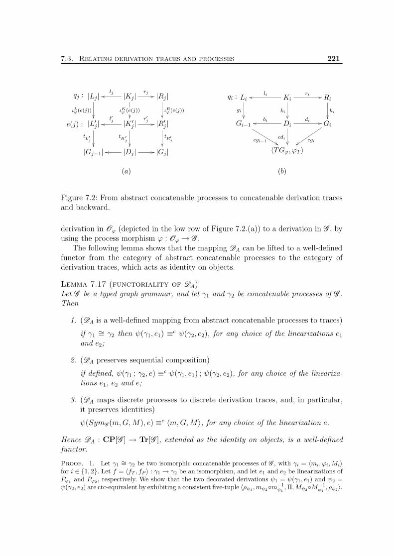
7.3. Relating derivation traces and processes 221
|Lj |qj :
ιLϕ(e(j))
|Kj |lj rj
ιKϕ (e(j))
|Rj |
ιRϕ (e(j))
|L′j |e(j) :
tL′j
|K ′j |l′j r′j
tK′j
|R′j |
tR′j
|Gj−1| |Dj | |Gj |
Liqi :
gi
Kili ri
ki
Ri
hi
Gi−1
cgi−1
Dibi di
cdi
Gi
cgi
〈TGϕ, ϕT 〉
(a) (b)
Figure 7.2: From abstract concatenable processes to concatenable derivation tracesand backward.
derivation in Oϕ (depicted in the low row of Figure 7.2.(a)) to a derivation in G , byusing the process morphism ϕ : Oϕ → G .
The following lemma shows that the mapping DA can be lifted to a well-definedfunctor from the category of abstract concatenable processes to the category ofderivation traces, which acts as identity on objects.
Lemma 7.17 (functoriality of DA)Let G be a typed graph grammar, and let γ1 and γ2 be concatenable processes of G .Then
1. (DA is a well-defined mapping from abstract concatenable processes to traces)
if γ1∼= γ2 then ψ(γ1, e1) ≡
c ψ(γ2, e2), for any choice of the linearizations e1and e2;
2. (DA preserves sequential composition)
if defined, ψ(γ1 ; γ2, e) ≡c ψ(γ1, e1) ; ψ(γ2, e2), for any choice of the lineariza-
tions e1, e2 and e;
3. (DA maps discrete processes to discrete derivation traces, and, in particular,it preserves identities)
ψ(SymG (m,G,M), e) ≡c 〈m,G,M〉, for any choice of the linearization e.
Hence DA : CP[G ] → Tr[G ], extended as the identity on objects, is a well-definedfunctor.
Proof. 1. Let γ1∼= γ2 be two isomorphic concatenable processes of G , with γi = 〈mi, ϕi,Mi〉
for i ∈ 1, 2. Let f = 〈fT , fP 〉 : γ1 → γ2 be an isomorphism, and let e1 and e2 be linearizations ofPϕ1 and Pϕ2 , respectively. We show that the two decorated derivations ψ1 = ψ(γ1, e1) and ψ2 =ψ(γ2, e2) are ctc-equivalent by exhibiting a consistent five-tuple 〈ρψ1 ,mψ2m
−1ψ1,Π,Mψ2M
−1ψ1, ρψ2〉.

222 Chapter 7. Concatenable Graph Processes
First, it is quite easy to recognize that Items(ψi) (see Definition 7.12) is isomorphic toItems(TGϕi
), for i ∈ 1, 2 and thus fT : TGϕ1 → TGϕ2 induces, in an obvious way, an iso-morphism ξ : Items(ψ1)→ Items(ψ2).
Since the restrictions of fT to the source and target graphs of the processes are isomorphisms,we can take
hσ = fT |•ϕ1: •ϕ1 → •ϕ2 and hτ = fT |ϕ1
• : ϕ1• → ϕ2
•,
which are compatible with mψ2 m−1ψ1
and Mψ2 M−1ψ1
, by definition of isomorphism of concatenableprocesses (and obviously compatible with ξ). Finally we can define the permutation Π : #ψ1 → #ψ2
as Π = e−12 fP e1.
Now, it is not difficult to check that 〈ρψ1 ,mψ2 m−1ψ1,Π,Mψ2 M
−1ψ1, ρψ2〉 is a consistent five-
tuple. Thus, by Theorem 7.14.(1), we conclude that ψ1 ≡c ψ2.
2. Let γ1 = 〈m1, ϕ1,M1〉 and γ2 = 〈m2, ϕ2,M2〉 be two concatenable processes such that theirsequential composition is defined, i.e., ϕ1
• = •ϕ2, M1 = m2 and all other items in γ1 and γ2 aredistinct. Let γ = 〈m1, ϕ,M2〉 be their sequential composition. Let us fix linearizations e1, e2 ande of Pϕ1 , Pϕ2 and Pϕ, respectively, and let ψ1 = ψ(γ1, e1), ψ2 = ψ(γ2, e2) and ψ = ψ(γ, e).
Observe that σ(ψ) = σ(ψ1) = σ(ψ1 ; ψ2) and similarly τ(ψ) = τ(ψ2) = τ(ψ1 ; ψ2). Further-more, we have that Items(ψ) and Items(ψ1;ψ2) are (isomorphic to) Items(TGϕ) = Items(TGϕ1)∪ Items(TGϕ2). Therefore one can verify that the five-tuple 〈ρψ, idσ(ψ),Π, idτ(ψ), ρψ1 ;ψ2〉, whereΠ = (e1 ∪ e2)−1 e is consistent (the function ξ being identity on classes). This fact, together withthe observation that mψ = mψ1 = mψ1;ψ2 and Mψ = Mψ2 = Mψ1;ψ2 , allows us to conclude, byTheorem 7.14.(1), that ψ ≡c ψ1;ψ2.
3. Obvious. 2
The backward step, from concatenable derivation traces to processes, is per-formed via a colimit construction that, applied to a decorated derivation ψ, essen-tially constructs the type graph as a copy of the source graph plus the items createdduring the rewriting process. Productions are instances of production applications.
Definition 7.18 (from traces to processes)Let G = 〈TG,Gs, P, π〉 be a typed graph grammar and let ψ = 〈m, ρ,M〉 be adecorated derivation, with #ψ = n. We associate to ψ a concatenable process cp(ψ) =〈m′, ϕ,M ′〉, defined as follows:
• 〈TGϕ, ϕT 〉 is a colimit object (in category TG-Graph) of the diagram rep-resenting derivation ψ, as depicted (for a single derivation step) in Fig-ure 7.2.(b);
• Pϕ = 〈prod(ψ)(j), j〉 | j ∈ n. For all j ∈ n, if prod(ψ)(j) = qis (inthe notation of Definition 5.11, Figure 5.6), then πϕ(〈prod(ψ)(j), j〉) is es-sentially production qis, but typed over TGϕ (see Figure 7.2.(b)). Formallyπϕ(〈prod(ψ)(j), j〉) is the production
〈|Lqis|, cgi−1 gi inLis〉
lqis← 〈|Kqis|, cdi ki inKqis〉rqis→ 〈|Rqis|, cgi hi in
Rqis〉

7.3. Relating derivation traces and processes 223
and ϕP (〈prod(ψ)(j), j〉) = prod(ψ)(j). Finally the “ι component” is given byιϕ(〈prod(ψ)(j), j〉) = 〈id|Lqis |, id|Kqis |, id|Rqis |〉.
Note that for j1 6= j2 we may have prod(ψ)(j1) = prod(ψ)(j2); instead, theproductions in Pϕ are all distinct, as they can be considered occurrences ofproduction of G ;
• notice that •ϕ = cg0(G0) and ϕ• = cgn(Gn) (and the cgi’s are injective, becauseso are the horizontal arrows) so that we can define m′ = cg0 m and M ′ =cgn M .
Finally we define the image of the trace [ψ]c as CA([ψ]c) = [cp(ψ)].
As an example, the process of Figure 7.1 can be obtained (up to isomorphism) byapplying the construction just described to either the derivation of Figure 5.6 orthat of Figure 5.11.
Notice that it is quite easy to have a concrete characterization of the colimit graphTGϕ. Since all the squares in the diagram representing derivation ψ : G0 ⇒
∗ Gn
commute (they are pushouts), TGϕ can be regarded equivalently as the colimit of
the bottom line of the derivation, G0b1← D1
d1→ G1b2← · · ·Dn
dn→ Gn. Thus TGϕ can becharacterized explicitly as the graph having as items Items(ρψ) (see Definition 7.12),and where source and target functions are determined in the obvious way. Theinjections cxi (x ∈ g, d) simply map every item into its equivalence class.
Lemma 7.19 (CA is well-defined)Let G = 〈TG,Gs, P, π〉 be a typed graph grammar and let ψ1 ≡
c ψ2 be two decoratedderivations of G . Then cp(ψ1) ∼= cp(ψ2).
Proof. Let ψ1 and ψ2 be ctc-equivalent decorated derivations of G . Then, by Theorem 7.14 thereexists a five-tuple 〈ρψ1 ,mψ2 m
−1ψ1,Π,Mψ2 M
−1ψ1, ρψ2〉 with a function ξ : Items(ψ1)→ Items(ψ2)
witnessing its consistence.Let cp(ψ1) = γ1 = 〈m1, ϕ1,M1〉 and cp(ψ2) = γ2 = 〈m2, ϕ2,M2〉. First notice that Items(ψi)
is isomorphic to the set of items of the corresponding type graph TGϕi(i ∈ 1, 2), and thus ξ
induces readily a function fT : TGϕ1 → TGϕ2, which, by definition of consistent five-tuple, isconsistent with the decorations of the processes. Moreover the permutation Π induces a bijectionfP : Pϕ1 → Pϕ2 , defined as fP (〈prod(ψ1)(j), j〉) = 〈prod(ψ2)(Π(j)),Π(j)〉, for j ∈ |Pϕ1 |.
From the definition of consistent five-tuple it follows easily that 〈fT , fP 〉 : γ1 → γ2 is anisomorphism of concatenable processes. 2
The next lemma shows that the constructions performed by CA and DA are, atabstract level, “inverse” to each other.
Lemma 7.20 (relating CA and DA)Let G be a graph grammar. Then:
1. CA(DA([γ])) = [γ], for any concatenable process γ;
2. DA(CA([ψ]c)) = [ψ]c, for any decorated derivation ψ.

224 Chapter 7. Concatenable Graph Processes
Proof. 1. Let γ = 〈m, p,M〉 be a concatenable process of G and let e : |Pϕ| → Pϕ be alinearization of Pϕ. Consider the decorated derivation:
ψ(γ, e) = 〈m, Gi−1 ⇒e(i) Gii∈|Pϕ|,M〉
as in Definition 7.16.Let us now construct the process γ1 = cp(ψ) = 〈m1, ϕ1,M1〉 as in Definition 7.18, with the
type graph TGϕ1 obtained as colimit of the diagram:
Liqi :
ιLϕ(e(i))
Ki
ιKϕ (e(i))
Ri
ιRϕ (e(i))
L′ie(i) :
tli
K ′i
tki
R′i
tri
Gi−1
cgi−1
Dibi di
cdi
Gi
cgi
TGϕ1
Observe that a possible concrete choice for TGϕ1 is TGϕ, with all cgi’s defined as inclusions.If we define fP : Pϕ1 → Pϕ as fP (〈prod(ψ)(i), i〉) = e(i), for i ∈ #ψ, then it is easy to prove
that f = 〈idTGϕ, fP 〉 : γ1 → γ is a concatenable process isomorphism.
2. First of all, if ψ is a discrete decorated derivation, the result is obvious. Otherwise we cansuppose ψ = 〈m, Gi−1 ⇒qi
Gii∈n,M〉 to be a derivation using a single production at each step(recall that, by Lemma 7.19, we can apply the concrete construction to any derivation in the traceand that in [ψ]c a derivation of this shape can always be found).
Let γ = cp(ψ) = 〈m, p,M〉 be the concatenable process built as in Definition 7.18. In particular,
the type graph TGϕ is defined as the colimit of the diagram:
Liqi :
gi
Kili ri
ki
Ri
hi
Gi−1
cgi−1
Dibi di
cdi
Gi
cgi
TGϕ
The set of productions is Pϕ = q′i = 〈qi, i〉 | i ∈ n, with πϕ(q′i) = 〈|Li|, cgi−1 gi〉li←
〈|Ki|, cdi ki〉ri→ 〈|Ri|, cgi ri〉. Moreover m = cg0 mψ and M = cgn Mψ. Remember that all
cgi’s are injections and cg0 : G0 → •ϕ, cgn : Gn → ϕ• are isomorphisms.Now it is not difficult to verify that prod(ψ) is a linearization of Pϕ and ψ′ = ψ(γ, prod(ψ)) is
the derivation whose ith step is depicted below.
Liq′i :
cgi−1gi
Ki
cdiki
Ri
cgihi
cgi−1(Gi−1) cdi(Di) cgi(Gi)
The family of isomorphism θXi: Xi → X ′
i | X ∈ G,D, i ∈ n∪θG0 between correspondinggraphs in the two (linear) derivations defined as:

7.4. Relating unfolding and deterministic processes 225
θDi= cdi and θGi
= cgi
satisfies the conditions of Definition 5.16 and thus we have that ψ′ ≡abs ψ. Therefore [ψ]c = [ψ′]c =DA([γ]) = DA(CA([ψ]c). 2
The previous lemma, together with functoriality of DA, allows us to concludethat CA : Tr[G ]→ CP[G ], defined as identity on objects and as CA([ψ]c) = [cp(ψ)]on morphisms, is a well-defined functor. In fact, given two decorated derivations ψ1
and ψ2, we have
CA([ψ1]c ; [ψ2]c) = [by Lemma 7.20.(2)]
= CA(DA(CA([ψ1]c)) ; DA(CA([ψ2]c))) = [by functoriality of DA]
= CA(DA(CA([ψ1]c) ; CA([ψ2]c))) = [by Lemma 7.20.(1)]
= CA([ψ1]c) ; CA([ψ2]c)
Similarly one proves also that CA preserves identities. Moreover, again byLemma 7.20, functors DA and CA are inverse to each other, thus implying the mainresult of this section.
Theorem 7.21 (relating processes and traces)Let G be a graph grammar. Then DA : CP[G ] → Tr[G ] and CA : Tr[G ] → CP[G ]are inverse to each other, establishing an isomorphism of categories. 2
7.4 Relating unfolding and deterministic pro-
cesses
This section is aimed at reconciling the unfolding semantics of a graph grammar,which basically relies on the notion of nondeterministic graph process, with thesemantics defined in terms of (concatenable) deterministic graph processes. Thegeneral pattern is the same we already followed in the case of nets. We show thatthe domain extracted from the unfolding of a grammar can be characterized as theset of deterministic processes with source in the start graph of the grammar andordered by prefix, or, formally, that Idl(〈[Gs] ↓ CP[G ]〉) is isomorphic to the domainLi(Eg(Ug(G ))) (see Sections 6.3-6.5 in the previous chapter).
The result can be proved for general (consuming) graph grammars, and notonly for the subclass of semi-weighted graph grammars. In fact, as usual, a centralrole in the proof is played by the characterization of the unfolding as a universalconstruction. We know from the previous chapter (Section 6.4) that, when consid-ering general morphisms, such a characterization only holds for the subcategory ofsemi-weighted grammars. However, limiting our attention to the (lluf) subcategoriesGGR and O-GGR where the left component of the type span of any morphism ismono (see Definition 6.25), the result generalizes to general (consuming) grammars.Simply observing that strong grammars morphisms (see Definition 6.12), which are

226 Chapter 7. Concatenable Graph Processes
used to define graph processes, are particular morphisms in GGR, it results clearthat the proof schema followed in the First Part for nets can be easily adaptedhere to reach the desired result for general grammars.
The first observation regards the structure of the category 〈[Gs] ↓ CP[G ]〉, which,by definition of sequential composition between processes, can be easily shown tobe a preorder.
Proposition 7.22Let G be a consuming grammar. Then the category 〈[Gs] ↓ CP[G ]〉 is a preorder.
Let . be the preorder relation in 〈[Gs] ↓ CP[G ]〉. As in the case of nets, giventwo concatenable processes γ : [Gs] → [G] and γ′ : [Gs] → [G′], if γ . γ′ . γ,then γ can be obtained from γ′ simply by composing it with a discrete process.Hence the partial order induced by 〈[Gs] ↓ CP[G ]〉 intuitively consists of classesof processes which are “left-isomorphic”, in the sense that they are related by aprocess isomorphism which is required to be consistent only with the decoration ofthe source.
The above considerations provide some intuition on the transformation definedbelow, which associates to each concatenable process γ a (non concatenable) markedprocess γ by forgetting the decoration of the target and using the decoration of thesource to construct the “ι” component for the start graph.
Definition 7.23 (from concatenable processes to marked processes)Let G = 〈TG,Gs, P, π〉 be a graph grammar and let φ : Gs → Can(Gs) be a fixedisomorphism. For any (abstract) concatenable process γ = 〈m,ϕ,M〉 : [Gs] → [G]let γ be the marked process ϕ obtained from the unmarked process ϕ by adding ascomponent ιsϕ the isomorphism m φ.
One can show that, for a fixed isomorphism φ, the above function establishes abijective correspondence between the elements of the partial order induced by thepreorder 〈[Gs] ↓ CP[G ]〉 and (finite) abstract marked processes.
Recall that the domain semantics of a graph grammar G , as defined in theprevious chapter, is obtained by taking the domain of configurations of the eventstructure associated to the unfolding Ug(G ) of the grammar. In symbols the domainis Li(Ea(Ug(G ))). We next prove the announced result, characterizing the domainsemantics in terms of the concatenable processes of a grammar.
Theorem 7.24 (unfolding vs. concatenable processes)Let G be a (consuming) graph grammar. Then the ideal completion of 〈[Gs] ↓ CP[G ]〉is isomorphic to the domain Li(Eg(Ug(G ))).
Proof (Sketch). Let G = 〈TG,P, π,Gs〉 be a graph grammar. As in the proof of the analogousresult for nets (see, e.g., Theorem 3.67), we exploit Lemma 3.66, which ensures that the thesisfollows form the existence of a surjective function ξ : 〈[Gs] ↓ CP[G ]〉 → K(Li(Eg(Ug(G )))) suchthat ξ is monotone and monic, namely for all γ1, γ2 in 〈[Gs] ↓ CP[G ]〉,
γ1 . γ2 iff ξ(γ1) ⊑ ξ(γ2).

7.4. Relating unfolding and deterministic processes 227
Recalling that the compact elements of the domain Li(Eg(Ug(G ))), associated to G , are exactlythe finite configurations of Eg(Ug(G )), we can define the function ξ as follows. Let γ = 〈m,ϕ,M〉 bea concatenable process in 〈[Gs] ↓ CP[G ]〉 and consider the marked process γ as in Definition 7.23.
By definition of graph process, γ : Oγ → G is a (marked) strong morphism. Therefore, byTheorem 6.26, there exists a unique arrow ϕ′ : Oγ → Ua(N), making the diagram below commute.
Ug(G )ϕG
G
Oγ
ϕ′
γ
Then the configuration associated to γ can be defined as ξ(γ) = ϕ′P (Pγ). The proof that ξ is a
well-defined surjective, monotone and monic function is routine. 2
The above result can be informally interpreted by saying that the elements ofthe domain associated to a graph grammar corresponds to the marked processes ofthe grammar, namely to the deterministic computations starting form the initialstate. Performing a further step, we can consider the pes associated to the abovedomain by Winskel’s equivalence, namely P(Li(Eg(Ug(G )))). The events of suchpes are special configurations which represent the possible histories of events in theies Eg(Ug(G )). Hence they correspond to processes where there is a production qwhich is maximum with respect to ր∗, namely computations where there is a “lastapplied” production q which cannot be shifted backward.


Chapter 8
Relating Some Event StructureSemantics for DPO GraphTransformation
This chapter briefly reviews two other prime event structure semantics which havebeen proposed in the literature for dpo graph transformation systems. The first one[CEL+96b] is built on top of the “abstract truly concurrent model of computation”of a grammar, i.e., the category of concatenable derivation traces. The other one[Sch94] is based on a deterministic variation of the dpo approach. By the results inChapters 6 and 7, these two alternative event structures can be shown to coincidewith the one obtained from the unfolding, which thus can be claimed to be “the”event structure semantics of dpo graph transformation.
8.1 Event structure from concatenable traces
The construction of a prime event structure for a (consuming) graph grammarproposed by Corradini et al. in the paper [CEL+96b], relies on the categoryTr[G ] of (concatenable) derivation traces (see Section 5.2). More precisely the au-thors consider the category of objects of Tr[G ] under the start graph Gs, namely〈[Gs] ↓ Tr[G ]〉, thought of as a synthetic representation of all the possible concurrentcomputations of the grammar beginning from the start graph. For consuming gram-mars, the partial order Dom[G ] obtained as the ideal completion of the preorder cat-egory 〈[Gs] ↓ Tr[G ]〉 is shown to have the desired algebraic structure, namely to be aprime algebraic, coherent and finitary partial order. Then, by Winskel’s results pre-sented in Section 2.4, Dom[G ] indirectly determines a pes, ES[G ] = P(Dom[G ]),which is assumed to give the concurrent semantics of G .
By the results in the previous chapter it is quite easy to recognize that ES[G ]coincides with the prime event structure extracted from the unfolding, namelyP(Li(Eg(Ug(G )))). In fact, by Theorem 7.21, for any grammar G , the category

230 Chapter 8. Relation with Other Event Structure Semantics
of concatenable processes CP[G ] and that of concatenable derivation traces Tr[G ]are isomorphic, and thus also the corresponding comma categories 〈[Gs] ↓ Tr[G ]〉and 〈[Gs] ↓ CP[G ]〉 are isomorphic. Therefore Theorem 7.24 immediately entailsthe desired result.
In [CEL+96b] the algebraic properties of the domain Dom[G ] are proved bypresenting an explicit construction of the prime event structure ES[G ] associated toa graph grammar and then by showing that the finite configurations of ES[G ] areone-to-one with the finite elements of the domain Dom[G ]. We briefly outline theconstruction of ES[G ], since we think that it is an interesting complement to theconstruction in Chapter 6. In fact, it provides an equivalent trace-based descriptionof the prime event structure associated to a grammar, which, in our opinion, can behelpful to get a clearer understanding of the meaning of the events in such pes.
Definition 8.1 (pes from traces)Let G = 〈TG,Gs, P, π〉 be a graph grammar. A pre-event for G is a pair 〈ψ, α〉,where ψ is a decorated derivation starting from a graph isomorphic to Gs, and α isa direct derivation which applies a single production in P (namely #α = 1) suchthat
1. ψ ; α is defined (i.e., τ(ψ) = σ(α), and Mψ = mα) and
2. ψ ; α ≡cΠ ψ′ implies Π(#ψ + 1) = #ψ + 1.
If 〈ψ, α〉 is a pre-event, we denote by εψα the corresponding derivation trace, namelyεψα = [ψ ; α].An event ε for G is then defined as a derivation trace ε = εψα for some pre-event〈ψ, α〉. For each event ε let Der(ε) denote the set of derivations containing suchevent, formally defined as:
Der(ε) =⋃δ | ∃δε ⊆ ε. ∃δ′. δε; δ
′ = δ.
Notice that, in particular, ε ⊆ Der(ε), since each concatenable derivation traceδε ⊆ ε can be concatenated with (the concatenable trace corresponding to) a discretederivation. Then the prime event structure of grammar G , denoted by ES[G ], isthe triple ES[G ] = 〈E,≤,#〉, where E is the set of all events for G , ε ≤ ε′ ifDer(ε′) ⊆ Der(ε), and ε#ε′ if Der(ε) ∩Der(ε′) = ∅.
Conceptually, an event εψα of a grammar G is determined by the application ofa production to a graph reachable from the start graph of G (i.e., by the directderivation α), together with the history that generated the graph items needed bythat production application (i.e., the derivation ψ). The fact that in the pre-event〈ψ, α〉 the last step α cannot be shifted backward (requirement (2) for pre-events)guarantees that α is not independent from all the previous steps in ψ. It is worthstressing that the same requirement implies that if ψ ; α ≡cΠ ψ
′ then ψ′ = ψ′′ ; α′ withψ ≡cΠ|#ψ
ψ′′ and α ≡abs α′. Clearly, isomorphic production applications or different

8.1. Event structure from concatenable traces 231
linearizations of the same history should determine the same event. Therefore anevent is defined as a set of equivalent derivations in G , more precisely as a traceincluding all the derivations having (a copy of) α as last step and containing thecorresponding history.
Given this notion of event, the causality and conflict relations are easily de-fined. In fact, considering for each event ε the set Der(ε) of all the derivations thatperformed ε at some point, we have that two events are in conflict if there is noderivation that can perform both of them, and they are causally related if eachderivation that performs one also performs the other.
Example 8.2 (event structure of grammar C -S )Figure 8.1 depicts part of the event structure of the graph grammar C -S of Example5.9. Continuous arrows form the Hasse diagram of the causality relation, while dottedlines connect events in direct conflict (inherited conflicts are not drawn explicitly).
Recalling that, intuitively, an event of a grammar corresponds to a specific ap-plication of a production together with its “history”, a careful analysis of grammarC -S allows us to conclude that its event structure contains the following events:
E = req(n) | n ∈ N ∪ ser(w), rel(w) | w ∈ N⊗,
where N⊗ denotes the set of non-empty sequences of distinct natural numbers.
In fact, an application of production REQ only depends on previous applicationsof the same production (because it consumes a job edge, and only REQ can pro-duce such edges). Therefore a natural number is sufficient to represent its history:conceptually, req(n) is the event corresponding to the n-th application of REQ. Anapplication of production SER, instead, depends both on a specific application ofREQ (because it consumes a req edge), and, because of the S node it consumesand produces, either on the start graph or on a previous application of SER itselffollowed by REL (SER cannot be applied in presence of a busy edge connected tonode S because of the dangling condition). It is not difficult to check that such anevent is uniquely determined by a non empty sequence of distinct natural numbers:ser(n1n2 · · ·nk) is the event corresponding to the application of SER which servesthe nk-th REQuest, after requests n1, . . . , nk−1 have been served in this order. Inturn, an application of production REL only depends on a previous application ofSER (because of the busy edge), and we denote by rel(w) the event caused directlyby ser(w).
This informal description should be sufficient to understand the part of the pesES[C -S ] shown in Figure 8.1, including only the events which are caused by thefirst three requests and the relationships among them. The causality and conflictrelations of ES[C -S ] are defined as follows:
• req(n) ≤ req(m) iff n ≤ m;
• req(n) ≤ ser(w) iff n ∈ w, that is, an application of SER only depends on therequest it serves and on those served in its history;
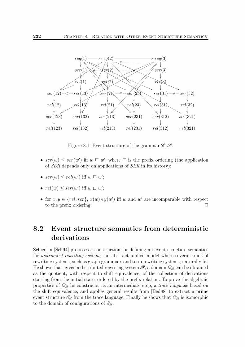
232 Chapter 8. Relation with Other Event Structure Semantics
req(1) req(2) req(3)
ser(1) #
#
ser(2) # ser(3)
rel(1) rel(2) rel(3)
ser(12) # ser(13) ser(21) # ser(23) ser(31) # ser(32)
rel(12) rel(13) rel(21) rel(23) rel(31) rel(32)
ser(123) ser(132) ser(213) ser(231) ser(312) ser(321)
rel(123) rel(132) rel(213) rel(231) rel(312) rel(321)
Figure 8.1: Event structure of the grammar C -S .
• ser(w) ≤ ser(w′) iff w ⊑ w′, where ⊑ is the prefix ordering (the applicationof SER depends only on applications of SER in its history);
• ser(w) ≤ rel(w′) iff w ⊑ w′;
• rel(w) ≤ ser(w′) iff w ⊏ w′;
• for x, y ∈ rel, ser, x(w)#y(w′) iff w and w′ are incomparable with respectto the prefix ordering. 2
8.2 Event structure semantics from deterministic
derivations
Schied in [Sch94] proposes a construction for defining an event structure semanticsfor distributed rewriting systems, an abstract unified model where several kinds ofrewriting systems, such as graph grammars and term rewriting systems, naturally fit.He shows that, given a distributed rewriting system R, a domain DR can be obtainedas the quotient, with respect to shift equivalence, of the collection of derivationsstarting from the initial state, ordered by the prefix relation. To prove the algebraicproperties of DR he constructs, as an intermediate step, a trace language based onthe shift equivalence, and applies general results from [Bed88] to extract a primeevent structure ER from the trace language. Finally he shows that DR is isomorphicto the domain of configurations of ER .

8.2. Event structure semantics from deterministic derivations 233
The main interest in Schied’s paper is for the application to graph grammars. Letus sketch how, according to Schied, the above construction instantiates to the caseof graph grammars. Graph grammars are modelled as distributed rewriting systemsby considering a deterministic variation of the dpo approach, where at each directderivation the derived graph is uniquely determined by the rewritten graph, theapplied production and the match. The idea consists of working on concrete graphs,where each item records his causal history. Formally the definition of deterministicdirect derivation is as follows.
Definition 8.3 (deterministic derivation)Let q : Lq ← Kq → Rq be a production and let m : Lq → G be a match. Then adeterministic direct derivation G ;q,m H exists if m satisfies the gluing conditionsand
H = glue〈q,m〉(q,m,G)−m(Lq − l(Kq)).
Let G = 〈TG,Gs, P, π〉 be a typed graph grammar. A deterministic derivation in G isa sequence of deterministic direct derivations Gs ;q1,m1 G1 ;q2,m2 . . . ;qn,mn Gn,starting from the start graph and applying productions of G .
Actually the above definition instantiates the ideas of Schied to our setting whichis slightly different, in that we work with typed graph grammars. Moreover in theoriginal definition of Schied, since productions are nameless, the new items in Hare marked only with the morphism m. Here we have to add also to name of theproduction.
Let G1 ;q1,m1 G2 ;q2,m2 G3 be sequentially independent deterministic deriva-tions. A basic observation is that we can shift the applications of the two produc-tions without changing the matches, thus obtaining a new deterministic derivationG1 ;q2,m2 G
′2 ;q1,m1 G3. The construction of the domain of a grammar is then based
on the partial order of deterministic derivations endowed with the prefix relation,and on shift equivalence.
Definition 8.4 (Schied’s domain)The Schied’s domain for a consuming grammar G , denoted by DG , is defined asthe quotient, with respect to shift equivalence, of the partial order of deterministicderivations of a grammar G endowed with the prefix relation.
Now it is not difficult to prove that the (ideal completion of) Schied’s do-main coincides with the domain semantics for a grammar G , as defined in Chap-ter 6. More precisely, the domain of configurations of the unfolding of a grammarConf (Ug(G )) (or equivalently the domain of configurations of the ies associated toG , i.e., Li(Eg(Ug(G )))) is isomorphic to Idl(DG ).
Theorem 8.5For any (consuming) graph grammar G , the ideal completion of DG and the domainConf (Ug(G )) are isomorphic.

234 Chapter 8. Relation with Other Event Structure Semantics
Proof. Consider the function η : DG → Conf (Ug(G )), defined as
η([d]sh) = 〈qi,mi〉 | i ∈ n if d : Gs ;q1,m1 G1 ;q2,m2 . . . ;qn,mnGn.
Notice that the definition is independent from the particular choice of the representative d, sincethe shift construction does not change the pairs 〈qi,mi〉 in the derivation.
Vice versa given a configuration C ∈ Conf (Ug(G )), consider any linearization of C, compatiblewith the asymmetric conflict relation ր of the unfolding. Let q′1, . . . , q
′n such a linearization, and
suppose q′i = 〈qi,mi〉 for i ∈ n. Then (by correspondence between unfolding and deterministicprocesses, and by properties of deterministic processes) we can construct a derivation
dC : Gs ;q1,m1 G1 ;q2,m2 . . . ;qn,mnGn.
and different linearizations lead to shift equivalent derivations. Thus we can define a functionγ : Conf (Ug(G ))→ DG as γ(C) = [dC ]sh, for any configuration C.
Finally, it is not difficult to verify that the two functions are monotonic and that they areinverse each other, establishing an isomorphism between the two domains. 2

Final Remarks on Part II
The notions and results developed in the First Part for contextual and inhibitornets have been fruitfully exploited to provide dpo graph transformation systemswith a systematic theory of concurrency which reduces the gap existing betweenPetri nets and graph grammars.
The intuitive relationship between graph grammars and inhibitor nets, and theobservation that safe graph grammars can be encoded by means of inhibitor netshave guided us in the definition of a Winskel’s semantics for graph grammars. Thenotion of occurrence grammar and the unfolding construction, which can be ex-pressed as a categorical coreflection between suitable categories of graph grammarsand occurrence grammars, are introduced by following closely the approach used forinhibitor nets. Then, not surprisingly, inhibitor event structures turn out to be suf-ficiently expressive to represent the dependencies between events in graph grammarcomputations, and thus the unfolding can be naturally abstracted to an inhibitorevent structure and finally, by using the results in Chapter 4, to a prime algebraicdomain.
SW-GGUg
⊥ O-GGEg
IO
IESLi
Dom
Pi
P
∼ PESL
As in the case of inhibitor nets, Winskel’s construction has not been fully extendedto graph grammars since the passage from occurrence grammars to inhibitor eventstructures is not expressed as a coreflection.
The notion of nondeterministic graph process which arises from our theory (theprototypical example of process being the unfolding), turns out to be a generalizationof the deterministic processes of [CMR96].
Furthermore concatenable graph processes have been defined as a variation of the(deterministic finite) graph processes endowed with an operation of sequential com-position, and have been shown to provide a semantics for graph grammars which isequivalent to the classical truly concurrent semantics based on the shift-equivalence.More precisely, we proved that the category CP[G ] of concatenable processes ofa grammar G is isomorphic to the abstract truly concurrent model of computationbased on traces Tr[G ] [CMR+97, CEL+96b, BCE+99]. As already done for the otherformalisms in the First Part, we have also proved that the process semantics is

236 Final Remarks on Part II
strictly related to the unfolding semantics, in the sense that concatenable processesallow to recover the same domain extracted from the unfolding.
As a last result, we showed that the prime event structure extracted from theunfolding coincides both with the one in [CEL+96b], obtained via a comma categoryconstruction on the category of concatenable derivation traces, and with the onein [Sch94], based on a deterministic variant of the dpo approach. Nicely, this resultgives a unified view of the various event structure semantics for the dpo approachto graph transformation in the literature.

Chapter 9
Conclusions
In this thesis we singled out a general approach, inspired by the theory of ordinaryPetri nets, for the development of a truly concurrent semantics of a class of systems.The semantics describes the concurrent behaviour of the systems through severalmathematical structures at various levels of abstraction. The approach has beenapplied to contextual and inhibitor nets, two generalization of Petri nets in theliterature, and finally to graph transformation systems.
The core of the approach is an unfolding construction which, when applied to asystem, produces a single structure describing all the possible computations of thegiven system starting from its initial state. A more abstract representation of thebehaviour of the system is obtained from the unfolding by abstracting from the na-ture of the states and recording only the events and the dependencies among events.This leads to a semantics based on suitable event structure models (asymmetric andinhibitor event structures), extending Winskel’s prime event structure in order toallow for a faithful representation of the dependencies between events, without re-ducing them simply to causality and symmetric conflict. We developed a generaltheory of the mentioned event structure models, which allows one to recover, finally,a semantics in terms of more classical structures for concurrency like prime alge-braic domains or equivalently prime event structures. The approach also includesa notion of deterministic process which captures the deterministic computations ofthe system. Deterministic processes, endowed with a suitable a notion of sequentialcomposition, form a category which can be seen as a model of computation for thesystem at hand. The two approaches to the semantics based on the unfolding andon deterministic processes can be finally reconciled by showing that both allow torecover the same event structure for the system.
Besides the concrete results and constructions proposed for each single model,we think that an “informal” achievement of the thesis is the presentation and thetreatment of (generalized) Petri nets and graph grammars in a unified framework,where also graph grammars are seen as a kind of enriched nets. This allowed us touse net-theoretical concepts to reason on graph transformation systems, a possibilitywhich has been useful in extending constructions and results from nets to graph

238 Chapter 9. Conclusions
grammars. We believe that the mentioned uniform presentation of nets and graphgrammars can help net-theorists to get closer to graph grammars and thus cancontribute, in the next future, to transfer to graph grammars some of the verificationand modelling techniques existing for Petri nets.
A technical problem which remains open regards the possibility of fully extend-ing Winskel’s construction also to inhibitor nets and graph grammars, by expressingas a coreflection the whole semantical transformation leading from the category ofsystems to the category of domains. In fact, while the results on contextual netscan be considered completely satisfactory, in the case of inhibitor nets and graphgrammars the absence of a coreflection with the category of inhibitor event struc-tures suggests that the construction should still be improved. We observed that thisproblem cannot be overcome easily. A possible solution could be to look for a quitedifferent unfolding construction, producing, for instance, in the case of nets, a flownet [Bou90] rather than an occurrence net.
An aspect which has not been considered in the thesis is the abstract algebraiccharacterization of the model of computation of a system. Well established resultsexist for ordinary Petri nets, whose computations have been characterized in termsof monoidal categories [MM90, Sas96]. In the case of contextual nets a partial an-swer to the question is given in [GM98], where it is shown that the category CP[N ]of concatenable processes of a contextual net N can characterized as a (non full)subcategory of a free dgs-monoidal category (a variation of monoidal categories withnon-natural duplicator and co-duplicator) constructed over the net. For graph trans-formation systems the PhD thesis [Hec98] provides a characterization of the modelof computation of a grammar based on a pseudo-free construction in the setting ofdouble categories with finite horizontal colimits. The result relies on the interestingassumption that, while the state of a Petri net is naturally characterized as a freecommutative monoid, colimits are the right constructions for generating and com-posing graphs. A different solution has been proposed in [GHL99], where the concretemodel of computation of a dpo grammar is axiomatized via the construction of afree dgs-monoidal bicategory. However the problem of giving an axiomatization ofthe abstract model of computation of a grammar as a true free construction is stillunsolved and represents an interesting topic of future research.
We mentioned in the Introduction that a (concrete) truly concurrent seman-tics for a system represents the basis for defining more abstract observational seman-tics. For instance, history preserving bisimulation (HP-bisimulation) on P/T Petrinets [vGG89] is based on the notion of process and of deterministic event structureEv(ϕ) associated to a process ϕ. Roughly speaking, two nets N0 and N1 are HP-bisimilar if, for any process ϕ0 of N0 we can find a process ϕ1 of N1 such that theunderlying deterministic pes’s are isomorphic. Moreover whenever ϕ0 can performan action becoming a process ϕ′0, then also ϕ1 must be able to perform the sameaction becoming ϕ′1 and vice versa; the isomorphism between Ev(ϕ0) and Ev(ϕ1) isrequired to be extensible to an isomorphism between Ev(ϕ′0) and Ev(ϕ′1). Informally

239
this means that each event of a net can be simulated by an event of the other netwith the same causal history. Relying on the process semantics and on the proposedevent structure models we can easily define notions of history preserving bisimulationfor generalized nets and for graph transformation systems. According to the chosenclass of event structure models one obtains various notions of HP-bisimulation which“observe” a system at different levels of abstraction. Some preliminary results forcontextual nets are illustrated in [BCM00], where it is shown that the decidabilityresult for HP-bisimulation of ordinary nets extends also to contextual nets.
Furthermore, once an unfolding construction has been defined, a natural questionsuggested by the work initiated in [McM93] regards the possibility of extracting fromthe (possibly infinite) unfolding of a system a finite fragment which is still useful tostudy some relevant properties of the system. For a subclass of contextual nets, calledread persistent nets, a generalization of McMillan’s algorithm has been proposedin [VSY98]. We are confident on the possibility of further extending such result tothe whole class of semi-weighted contextual nets by relying on the notion of “possiblehistory” of a transition introduced in Chapter 3. However this extension could notbe relevant for concrete applications since the need of considering different historiesfor the same event could significantly increase the complexity of the algorithm.
Finally, as already mentioned, although in this thesis we have concentrated onlyon basic graph rewriting acting on directed (typed) graphs, it would be interesting tounderstand if the presented constructions and results can extended to more generalstructures. While the generalization to hypergraphs is trivial, developing a similartheory for more general structures and for abstract categories (e.g., high level re-placement systems [EHKPP91]) is not immediate and represents an interesting topicof further investigation.


Appendix A
Basic Category Theory
This appendix collects some basic notions of category theory which are used inthe thesis. For a comprehensive introduction to the subject we refer the readerto [ML71, BW90]. The notion of category represents a formalization of the intuitiveidea of a collection of objects with common structure, related by mappings whichpreserve such structure.
Definition A.1 (category)A category C consists of a collection OC of objects (ranged over by a, b,...) and acollection AC of arrows (ranged over by f , g,...) with the following structure:
• Each arrow has a domain dom(f) and a codomain cod(f) (also called sourceand target, respectively) that are objects. We write
f : a→ b or also af−→ b
if a is the domain of f and b is the codomain of f .
• Given two arrows f and g such that cod(f) = dom(g), the composition of fand g, written f ; g, is an arrow with domain dom(f) and codomain cod(g):
af−→ b
g−→ c = a
f ;g−→ c.
• The composition operator is associative, i.e.,
f ; (g; h) = (f ; g); h
whenever f , g and h can be composed.
• For every object a there is an identity arrow ida : a → a, such that for anyarrow f : a→ b
ida; f = f = f ; idb.

242 Appendix A. Basic Category Theory
The collection of arrows from an object a to an object b in C, called homset, isdenoted by C[a, b].
As usual, we write either f ∈ AC or just f ∈ C to say that f is an arrow in C, andsimilarly for objects.
Example A.2 (category Set)We denote by Set the category whose objects are sets and whose arrows are totalfunctions, with the ordinary composition of functions as arrow composition and theidentity function idX as identity for each set X.
Example A.3 (categories and preorders)Recall that a preorder is a set X together with a binary relation ≤ which is reflexiveand transitive. A preorder (X,≤) can be seen as a category X where the objects arethe elements of X, and for any x, y ∈ X the homset X[x, y] is a singleton if x ≤ yand the empty set otherwise.
Conversely, a category A where there is at most one arrow between any twoobjects is called a preorder category or simply a preorder. It will be often identifiedwith the underlying preordered set (AO,≤), with a ≤ b iff |A[a, b]| = 1.
Other examples are the empty category 0, the category 1 with one object • andone arrow id•, and the category of sets and relations. A category is called discreteif every arrow is the identity of some object. For example, 1 is a discrete category.
Definition A.4 (subcategory)Given two categories A and B, we say that A is a subcategory of B, if
• OA ⊆ OB,
• for all a, b ∈ OA, A[a, b] ⊆ B[a, b],
• composition and identities in A coincide with those in B.
The subcategory A is called full if A[a, b] = B[a, b], for all a, b ∈ OA. The subcategoryA is called lluf if it has the same objects of A, namely if OA = OB.
In category theory, it is common practice to express properties or requirementsby means of commutative diagrams. A diagram is made up of objects and arrows,and we say that it commutes if picking any two objects in the diagram and tracingany path of arrows from one object to the other, the composition of the arrowsyields always the same result. For example, the associativity of composition canbe equivalently expressed by saying that the diagram (i) in Figure A.1 commutes.Similarly, the identities are characterized by the commutativity of the diagram (ii)in Figure A.1.

A.1. Functors 243
af ;g
f
b
h
c
g
g;hd
af
fida
b
idb
af
b
(i) (ii)
Figure A.1: Associativity and identity diagrams for arrow composition.
Definition A.5 (inverse)An arrow f : a → b in a category C is called an isomorphism if there is an arrowg : b→ a such that f ; g = ida and g; f = idb. In this case, g is called the inverse of f(and vice versa) and it is denoted by f−1 (it is immediate to prove that the inverse,if it exists, is unique).
The set-theoretic notions of injective and surjective function are captured by thecategorical concepts of mono and epi morphism.
Definition A.6 (mono and epi morphisms)An arrow m : b→ c in a category C is called a monomorphism, or simply mono, iffor any pair of morphisms f, g : a→ b, f ;m = g;m implies f = g.
Conversely, e : a→ b is called an epimorphism, or simply epi, if for any pair ofmorphisms f, g : b→ c, e; f = e; g implies f = g.
A.1 Functors
Functors are essentially morphisms between categories, in the sense that they aremappings which “preserve” the relevant structure of categories.
Definition A.7 (functor)Given two categories A and B, a functor F : A→ B consists of a pair of mappings(FO, FA) such that:
• FO : OA → OB,
• FA : AA → AB,
• if f : a→ b ∈ A then FA(f) : FO(a)→ FO(b) (but usually we omit subscriptsand write F (f) : F (a)→ F (b)),
• F (f ; g) = F (f);F (g) for each f : a→ b and g : b→ c ∈ A,
• F (ida) = idF (a) for each object a ∈ A.

244 Appendix A. Basic Category Theory
A notion of composition for functors is naturally defined via the compositionof their object and arrow components, seen as functions. It is easy to see that thisoperation is associative and admits identities, namely the (endo)functors IdA : A→A whose components are the identities on the sets of objects and arrows of A. Thisyields the category Cat of all categories, whose objects are categories and whosearrows are functors. Consequently a notion of isomorphism of categories (as objectsof Cat) naturally arises:
Definition A.8 (isomorphism of categories)Two categories A and B are isomorphic if there are two functors F : A → B andG : B→ A such that G F = IdA and F G = IdB.
Any functor F : A→ B induces a set mapping A[a, b]→ B[F (a), F (b)]. Accord-ing to the properties of such mapping, the next definition identifies special classesof functors.
Definition A.9 (faithful, full and embedding functors)A functor F : A→ B is called
• faithful if the induced mapping F : A[a, b] → B[F (a), F (b)] is injective forevery pair of objects a, b in A;
• full if the induced mapping F : A[a, b]→ B[F (a), F (b)] is surjective for everypair of objects a, b in A;
• an embedding if FA : AA → AB is injective.
Observe that an embedding is always injective on objects and faithful. Moreover,if it is also full it establishes an isomorphisms between A and the full subcategoryF (A) of B.
A.2 Natural transformations
Natural transformations can be thought of as morphisms between functors. A naturaltransformation from a functor F to a functor G respects the structure of the functorsin the sense that it provides a uniform way to translate images of objects and arrowsthrough F to images through G.
Definition A.10 (natural transformation)Let F,G : A→ B be two functors. A natural transformation η : F
·−→ G : A→ B
consists of a family of arrows in B indexed by the objects of A,
η = ηa : F (a)→ G(a) ∈ ABa∈OA
such that the diagram in Figure A.2 commutes for every arrow f : a → b ∈ A,expressing the naturality of the transformation η. The arrow ηa is called the com-ponent at a of the natural transformation η.

A.3. Universal properties, limits and colimits 245
a
f
F (a)ηa
F (f)
G(a)
G(f)
b F (b) ηbG(b)
Figure A.2: Naturality square of the transformation η : F·−→ G : A → B for the
arrow f ∈ A.
Two natural transformations η : F·−→ G and ν : G
·−→ H can be composed
elementwise, obtaining a natural transformation η ∗ ν : F·−→ H , with (η ∗ ν)a =
ηa; νa. Moreover, for each functor F : A → B there exists the obvious identitytransformation 1F : F
·−→ F given by 1F = idF (a)a∈OA
. This allows us to view thecollection of functors between two categories A and B as the objects of a category,where arrows are natural transformations, usually denoted BA and called functorcategory.
The notion of equivalence of categories allows one to express the fact that twocategories are “essentially the same”. Informally, two categories are equivalent ifthey only differ for the fact that isomorphic objects are “counted more than once”.Say that category C is skeletal two objects in C are isomorphic only if they areidentical, and call a skeleton of C a maximal skeletal full subcategory of C. It ispossible to prove that each category C has a skeleton and that any two skeletons ofC are isomorphic. Then two categories are called equivalent if they have isomorphicskeletons.
An alternative, more handy definition of equivalence can be given by using nat-ural transformations.
Definition A.11 (equivalence)Two categories A and B are equivalent if there are functors F : A → B andG : B → A, and two natural isomorphisms IdA ≃ F ;G and G;F ≃ IdB (where ≃denotes the natural isomorphism between functors).
A.3 Universal properties, limits and colimits
In category theory, several notions are often stated by means of universal properties,namely by requiring the existence of a unique arrow that verifies certain properties.
A very commonly used construction is that of product, generalizing the set-theoretical cartesian product.
Definition A.12 (product)We say that C has binary products if for any pair of objects a, b ∈ C there exists

246 Appendix A. Basic Category Theory
cf
〈f,g〉g
a a× bΠa Πb
b
a
f
inaa+ b
[f,g]
binb
g
c
(i) (ii)
Figure A.3: The diagrams for (i) products and (ii) coproducts.
an object a × b together with two projections Πa : a × b → a and Πb : a× b → bsatisfying the following condition:
for each object c and arrows f : c → a and g : c → b in C there existsa unique arrow 〈f, g〉 : c → a× b such that f = 〈f, g〉; Πa and g =〈f, g〉; Πb, i.e., there exists a unique arrow 〈f, g〉 : c → a× b such thatthe diagram (i) in Figure A.3 commutes (the fact that 〈f, g〉 is depictedas a dotted arrow expresses its universal property, i.e., that it exists andis unique).
The dual notion of product is called coproduct, and it generalizes the set-theoretical construction of disjoint sum.
Definition A.13 (coproduct)We say that C has binary coproducts if for any pair of objects a, b ∈ C there existsan object a + b together with two injections ina : a → a + b and inb : b → a + bsatisfying the following condition:
for each object c and arrows f : a→ c and g : b→ c in C there exists aunique arrow [f, g] : a+ b→ c such that ina; [f, g] = f and inb; [f, g] = g,i.e., there exists a unique arrow [f, g] : a+ b→ c such that the diagram(ii) in Figure A.3 commutes.
The product (resp. coproduct) of two objects a and b is often denoted simply bya× b (resp. a+ b), but notice that it is unique only up to isomorphism, and that itis uniquely determined only specifying also its projections (resp. injections).
Products and coproducts, as well as other useful notions like pullbacks, pushouts,equalizers, coequalizers, are all instances of the more general concept of limit andof its dual notion of colimit.
Given a category C, a diagram D in C can be thought of as a graph G whereeach node a is labelled by an object D(a) of C, and each edge e with source a andtarget b is labelled by an arrow D(e) : D(a)→ D(b). More precisely the diagram canbe seen as a graph morphism D : G→ C, where C stands for the graph underlyingthe category C. In this case we say that the diagram D has shape G.

A.3. Universal properties, limits and colimits 247
cpa pb
D(a)D(g)
D(b)
Figure A.4: Commutative cone.
c′
h
p′a c
pa
D(a)
Figure A.5: An arrow h from the cone p′ to p.
Definition A.14 (cone)Let C be a category and let D : G → C be a diagram in C with shape G. A coneover the diagram D is an object c of C together with a family paa∈G of arrows ofC indexed by the nodes of G, such that pa : c → D(a) for each node a of G. Thearrow pa is called the component of the cone at object a. We indicate the cone bywriting p : c→ D.
A cone is called commutative if for any arrow g : a → b ∈ G, the diagram inFigure A.4 commutes.1 If p′ : c′ → D and p : c → D are cones, an arrow from thefirst to the second is an arrow h : c′ → c such that for each node a ∈ G, the diagramin Figure A.5 commutes.
Definition A.15 (Limit)A commutative cone over the diagram D is called universal if every commutativecone over the same diagram has a unique arrow to it. A universal cone, if suchexists, is called a limit of the diagram D.
Example A.16A limit of the diagram (ca, cb) (i.e., a pair of objects), which is associated to thediscrete graph with only two nodes a and b, is an object u, together with two arrowsp1 : u→ ca and p2 : u→ cb, such that for any other cone (u′, p′1 : u′ → ca, p
′2 : u′ →
cb) there exists a unique arrow h : u′ → u with p′1 = h; p1 and p′2 = h; p2. Notice that
1We remark that the diagram D is not assumed to commute.

248 Appendix A. Basic Category Theory
d′ h′2
h′1
h
dh2
h1
b
g
af
c
cg
f
b
h2h′2
ah1
h′1
dh
d′
(i) (ii)
Figure A.6: Diagrams for (i) pullback and (ii) pushout.
this is just the definition of product of ca and cb. Dually, the colimit of the diagram(ca, cb) defines the coproduct of ca and cb (if it exists).
A very commonly used kind of (co)limit is given by pullbacks and pushouts.
Definition A.17 (pullback and pushout)Let G be the graph • • • . A diagram of this shape in a category C is givenby three objects a, b and c, and two morphisms f : a→ c and g : b→ c. A cone forsuch diagram is an object d together with three arrows h1 : d → a, h2 : d → b andh3 : d→ c, such that h3 = h1; f and h3 = h2; g. Hence, h1; f = h2; g and the cone isequivalently expressed by (d, h1, h2), because h3 is uniquely determined by h1 and byh2. The cone is universal if for any other cone (d′, h′1, h
′2) of the same diagram there
exists a unique arrow h : d′ → d making the diagram in Figure A.6.(i) commute. Alimit for this diagram (if it exists) is called a pullback of f and g.
The dual notion is called pushout. It can be defined as the colimit for the diagram(a, b, c, f : c → a, g : c → b), which is associated to the graph • • • .Figure A.6.(ii) represents the corresponding diagram.
An interesting property of pullbacks is the preservation of monomorphisms: ifthe arrow g in Figure A.6 is mono then also h1 is mono. Dually, pushouts preserveepimorphisms.
A.4 Adjunctions
Adjunctions are extensively used in the thesis to characterize constructions by meansof universal properties. There are several equivalent definitions of adjunction. Wethink that the more “intuitive” one relies on the scenario consisting of two categoriesA and B and a functor F : A→ B, where given an object b in B we want to find anobject u in F (A), i.e. u = F (Gb) for some object Gb in A, that better approximatesb. The intuitive idea of approximation is formalized by the existence of an arrow

A.4. Adjunctions 249
Gb
a
f
F (Gb)ǫb
b
F (a)
F (f)g
Figure A.7: The left adjoint F .
Gb′
Gb
h
F (Gb′)ǫb′
b′
F (Gb) ǫb
ǫb;fF (h)
b
f
Figure A.8: The definition of the right adjoint to F .
from F (Gb) to b. The fact that this approximation is better than the others meansthat any other arrow f : F (a) → b for some a in A factorizes through the betterapproximation of b via the image of a morphism in A, in a unique way.
Definition A.18 (adjunction)Given two categories A and B and a functor F : A → B, we say that F is aleft adjoint if for each object b in B there exists an object Gb in A and an arrowǫb : F (Gb)→ b in B such that for any object a ∈ A and for any arrow g : F (a)→ bthere exists a unique arrow f : a→ Gb ∈ A such that g = F (f); ǫb (see Figure A.7).
An immediate consequence of the fact that F is left adjoint is the existence ofa functor from B to A that maps each object b into its approximation Gb, i.e., themapping G extends to a functor. This point can be proved by noticing that, givenan arrow f : b→ b′ in B, the arrow ǫb; f : F (Gb)→ b′ factorizes through ǫb′ and theimage of a unique arrow h from Gb to Gb′ . Therefore the functor G can be definedby taking G(f) = h (see Figure A.8). The functor G is called the right adjoint to F ,and we write F ⊣ G. The collection ǫ = ǫbb∈B is called the counit of the adjunctionand defines a natural transformation from G;F to 1B.
Remark A.19Adjoints are unique up to natural isomorphism. This is the reason why we areallowed to speak of the right adjoint to F .
We could have employed an equivalent dual approach to the definition of adjoints,by starting with the functor G and defining the “least upper” approximation Fa foreach object a. This construction yields the unit η = ηa : a → G(Fa)a∈A of theadjunction (see Figure A.9).

250 Appendix A. Basic Category Theory
G(b)
a
f
ηaG(Fa)
G(g)
b
Fa
g
Figure A.9: The right adjoint G.
An important property of adjunctions is the preservation of universal construc-tions: left adjoints preserve colimits and right adjoints preserve limits.
Theorem A.20 (adjoints and (co)limits)Let F : A→ B be a right adjoint functor, let D : G→ A be a diagram in A and letp : c → D be the limit of D. Then F (p) : F (c) → F (D) is the limit of the diagramF (D) (defined as F (D)(x) = F (D(x)) for any x in G) in B.
A dual result holds for colimits and left adjoints.A typical example of adjunction consists of a forgetful functor U : S → C,
from a category S of certain structures and structure-preserving functions (e.g.,the category Mon of monoids and monoid homomorphisms) to a category C withless structure (e.g., Set). Forgetful functors have often a left adjoint that adds thestructure missing in C by means of a free construction.
Reflections and coreflections are two particularly important kinds of adjunction,where respectively the counit and the unit are natural isomorphisms. For instance,in the case of a coreflection, referring to the introductory discussion, we have thatB is equivalent to a full subcategory of A. Thus we can think that G gives thebest approximation of an object of A inside such a subcategory. Observe that anequivalence is an adjunction which is both a reflection and a coreflection.
A.5 Comma category constructions
Given two functors F : A → C and G : B → C, with a common target C we canconsider the comma category 〈F ↓ G〉. This is a standard categorical constructionwhich makes (a selected subset) of the arrows of C be objects of a new category. Moreprecisely, the objects of 〈F ↓ G〉 are arrows of the kind x : F (a)→ G(b) in C, and anarrow h : (x : F (a) → G(b)) → (y : F (a′) → G(b′)) is a pair (f : a→ a′, g : b → b′)of arrows in A and B, respectively, such that the diagram of Figure A.10 commutes.
Clearly, by varying the choice of F and G we obtain several different “commaconstructions”. Next we give an explicit definition of two relevant instances of commaconstruction. First if A is 1, then F just selects an object c in C. If moreover B = Cand G = IdC then 〈F ↓ G〉, denoted in this case by 〈c ↓ C〉, is the comma categoryof objects of C under c.

A.5. Comma category constructions 251
F (a)
x
F (f)F (a′)
y
G(b)G(g)
G(b)
Figure A.10: Arrows in the comma category 〈F ↓ G〉.
cyx
c′f
c′′
c′
x
fc′′
y
c
(i) (ii)
Figure A.11: Category of objects under/over a given object.
Definition A.21 (category of objects under a given object)Let C be a category and let c be an object of C. The category of objects (of C) underc, denoted 〈c ↓ C〉, has arrows like x : c → c′ as objects. Furthermore f : (x : c →c′)→ (y : c→ c′′) is an arrow of 〈c ↓ C〉 if f : c′ → c′′ is an arrow of C and x; f = y(see Figure A.11.(i)).
Dually, when F = IdC, B = 1 and G is the constant c, we obtain the categoryof objects over a given object.
Definition A.22 (category of objects over a given object)Let C be a category and let c be an object of C. The category of objects (of C) overc, denoted 〈C ↓ c〉, has arrows like x : c′ → c as objects. Furthermore f : (x : c′ →c)→ (y : c′′ → c) is an arrow of 〈C ↓ c〉 if f : c′ → c′′ is an arrow of C and x = f ; y(see Figure A.11.(ii)).
Interestingly, to obtain limits and colimits in the category 〈C ↓ c〉 one can considerthe corresponding diagram in C and compute the limit there. Hence 〈C ↓ c〉 inheritsfrom C the properties of being complete and cocomplete.


Bibliography
[AF73] T. Agerwala and M. Flynn. Comments on capabilities, limitations and“correctness” of Petri nets. Computer Architecture News, 4(2):81–86,1973.
[Age74] T. Agerwala. A complete model for representing the coordination ofasynchronous processes. Hopkins Computer Research Report 32, JohnHopkins University, 1974.
[BC88] G. Boudol and I. Castellani. Permutation of transitions: an event struc-ture semantics for CCS and SCCS. In Linear Time, Branching Timeand Partial Order Semantics in Logics and Models for Concurrency,volume 354 of LNCS, pages 411–427. Springer Verlag, 1988.
[BC96] R. Banach and A. Corradini. An opfibration account of typed DPOand DPB graph transformation: General productions. Technical ReportUMCS-96-11-2, University of Manchester, Department of ComputerScience, 1996.
[BCE+99] P. Baldan, A. Corradini, H. Ehrig, M. Lowe, U. Montanari, andF. Rossi. Concurrent Semantics of Algebraic Graph TransformationSystems. In G. Rozenberg, editor, Handbook of Graph Grammars andComputing by Graph Transformation, volume III: Concurrency, pages107–187. World Scientific, 1999.
[BCM98a] P. Baldan, A. Corradini, and U. Montanari. Concatenable graph pro-cesses: relating processes and derivation traces. In Proceedings ofICALP’98, volume 1443 of LNCS, pages 283–295. Springer Verlag,1998.
[BCM98b] P. Baldan, A. Corradini, and U. Montanari. An event structure seman-tics for P/T contextual nets: Asymmetric event structures. In M. Nivat,editor, Proceedings of FoSSaCS ’98, volume 1378 of LNCS, pages 63–80.Springer Verlag, 1998.

254 Bibliography
[BCM99a] P. Baldan, A. Corradini, and U. Montanari. Contextual Petri nets,asymmetric event structures and processes. Technical Report TR-99-18, Computer Science Department, University of Pisa, 1999.
[BCM99b] P. Baldan, A. Corradini, and U. Montanari. Unfolding and Event Struc-ture Semantics for Graph Grammars. In W. Thomas, editor, Proceed-ings of FoSSaCS ’99, volume 1578 of LNCS, pages 73–89. SpringerVerlag, 1999.
[BCM99c] P. Baldan, A. Corradini, and U. Montanari. Unfolding of double-pushout graph grammars is a coreflection. In G. Ehrig, G. Engels,H.J. Kreowski, and G. Rozenberg, editors, TAGT’98 Conference Pro-ceedings, volume 1764 of LNCS, pages 145–163. Springer Verlag, 1999.
[BCM00] P. Baldan, A. Corradini, and U. Montanari. History preserving bisim-ulations for contextual nets. In D. Bert and C. Choppy, editors,WADT’99 Conference Proceedings, number 1827 in LNCS, pages 291–310. Springer Verlag, 2000.
[BD87] E. Best and R. Devillers. Sequential and concurrent behaviour in Petrinet theory. Theoretical Computer Science, 55(1):87–136, 1987.
[BDKP91] E. Best, R. Devillers, A. Kiehn, and L. Pomello. Concurrent bisimula-tions in Petri nets. Acta Informatica, 28(3):231–264, 1991.
[Bed88] M.A. Bednarczyk. Categories of asynchronous systems. PhD thesis,University of Sussex, 1988. Report no. 1/88.
[Ber78] G. Berry. Stable models of typed lambda-calculi. In Proceedings of the5th ICALP, volume 62 of LNCS, pages 72–89. Springer-Verlag, 1978.
[BG00] R. Bruni and F. Gadducci. Algebraic properties of (Co)Spans. Toappear., 2000.
[BHMR98] F. Bueno, M. Hermenegildo, U. Montanari, and F. Rossi. Partial or-der and contextual net semantics for atomic and locally atomic CCprograms. Science of Computer Programming, 30:51–82, 1998.
[Bod98] C. Bodei. Some concurrency models in a categorical framework. InProceedings of ICTCS’98, pages 180–191. World Scientific, Prato 1998,1998.
[Bou90] G. Boudol. Flow Event Structures and Flow Nets. In Semantics ofSystem of Concurrent Processes, volume 469 of LNCS, pages 62–95.Springer Verlag, 1990.

Bibliography 255
[BP96] N. Busi and G. M. Pinna. Non Sequential Semantics for ContextualP/T Nets. In Application and Theory of Petri Nets, volume 1091 ofLNCS, pages 113–132. Springer Verlag, 1996.
[BP99] N. Busi and G. M. Pinna. Process semantics for Place/Transition netswith inhibitor and read arcs. Fundamenta Informaticae, 40(2-3):165–197, 1999.
[Bus98] N. Busi. Petri Nets with Inhibitor and Read Arcs: Semantics, Analysisand Application to Process Calculi. PhD thesis, University of Siena,Department of Computer Science, 1998.
[BW90] M. Barr and C. Wells. Category Theory for Computing Science. Pren-tice Hall, 1990.
[CEL+94a] A. Corradini, H. Ehrig, M. Lowe, U. Montanari, and F. Rossi. Abstractgraph derivations in the double-pushout approach. In H.-J. Schneiderand H. Ehrig, editors, Proceedings of the Dagstuhl Seminar 9301 onGraph Transformations in Computer Science, volume 776 of LNCS,pages 86–103. Springer Verlag, 1994.
[CEL+94b] A. Corradini, H. Ehrig, M. Lowe, U. Montanari, and F. Rossi. Noteon standard representation of graphs and graph derivations. In H.-J.Schneider and H. Ehrig, editors, Proceedings of the Dagstuhl Seminar9301 on Graph Transformations in Computer Science, volume 776 ofLNCS, pages 104–118. Springer Verlag, 1994.
[CEL+96a] A. Corradini, H. Ehrig, M. Lowe, U. Montanari, and J. Padberg. Thecategory of typed graph grammars and its adjunctions with categoriesof derivations. In J. Cuny, H. Ehrig, G. Engels, and G. Rozenberg, ed-itors, Proceedings of the 5th International Workshop on Graph Gram-mars and their Application to Computer Science, volume 1073 of LNCS.Springer Verlag, 1996.
[CEL+96b] A. Corradini, H. Ehrig, M. Lowe, U. Montanari, and F. Rossi. An eventstructure semantics for graph grammars with parallel productions. InJ. Cuny, H. Ehrig, G. Engels, and G. Rozenberg, editors, Proceedingsof the 5th International Workshop on Graph Grammars and their Ap-plication to Computer Science, volume 1073 of LNCS. Springer Verlag,1996.
[CH93] S. Christensen and N. D. Hansen. Coloured Petri nets extended withplace capacities, test arcs and inhibitor arcs. In M. Ajmone-Marsan,editor, Applications and Theory of Petri Nets, volume 691 of LNCS,pages 186–205. Springer Verlag, 1993.

256 Bibliography
[CMR96] A. Corradini, U. Montanari, and F. Rossi. Graph processes. Funda-menta Informaticae, 26:241–265, 1996.
[CMR+97] A. Corradini, U. Montanari, F. Rossi, H. Ehrig, R. Heckel, and M. Lowe.Algebraic Approaches to Graph Transformation I: Basic Concepts andDouble Pushout Approach. In G. Rozenberg, editor, Handbook of GraphGrammars and Computing by Graph Transformation. Volume 1: Foun-dations. World Scientific, 1997.
[Cor96] A. Corradini. Concurrent graph and term graph rewriting. In U. Mon-tanari and V. Sassone, editors, Proceedings of CONCUR’96, volume1119 of LNCS, pages 438–464. Springer Verlag, 1996.
[DFMR94] N. De Francesco, U. Montanari, and G. Ristori. Modeling ConcurrentAccesses to Shared Data via Petri Nets. In Programming Concepts,Methods and Calculi, IFIP Transactions A-56, pages 403–422. NorthHolland, 1994.
[DGV93] P. Degano, R. Gorrieri, and S. Vigna. On relating some models forconcurrency. In M. C. Gaudel and J. P. Jouannaud, editors, 4th Con-ference on Theory and Practice of Software Development, volume 668of LNCS, pages 15–30. Springer-Verlag, 1993.
[DMM89] P. Degano, J. Meseguer, and U. Montanari. Axiomatizing net com-putations and processes. In Proceedings of LICS’89, pages 175–185,1989.
[DMM96] P. Degano, J. Meseguer, and U. Montanari. Axiomatizing the algebraof net computations and processes. Acta Informatica, 33:641–647, 1996.
[EHKPP91] H. Ehrig, A. Habel, H.-J. Kreowski, and F. Parisi-Presicce. Parallelismand concurrency in High-Level Replacement Systems. MathematicalStructures in Computer Science, 1:361–404, 1991.
[Ehr79] H. Ehrig. Introduction to the algebraic theory of graph grammars. InV. Claus, H. Ehrig, and G. Rozenberg, editors, Proceedings of the 1stInternational Workshop on Graph-Grammars and Their Applicationto Computer Science and Biology, volume 73 of LNCS, pages 1–69.Springer Verlag, 1979.
[Ehr87] H. Ehrig. Tutorial introduction to the algebraic approach of graph-grammars. In H. Ehrig, M. Nagl, G. Rozenberg, and A. Rosen-feld, editors, Proceedings of the 3rd International Workshop on Graph-Grammars and Their Application to Computer Science, volume 291 ofLNCS, pages 3–14. Springer Verlag, 1987.

Bibliography 257
[EKT94] H. Ehrig, H.-J. Kreowski, and G. Taentzer. Canonical derivations forhigh-level replacement systems. In [SE94], pages 153–169, 1994.
[GHL99] F. Gadducci, R. Heckel, and M. LLabres. A bicategorical axioma-tization of concurrent graph rewriting. In Proceedings of CTCS’99,volume 7 of ENTCS. Elsevier, 1999.
[GM98] F. Gadducci and U. Montanari. Axioms for contextual net processes.In Proceedings of ICALP’98, volume 1443 of LNCS, pages 296–308.Springer Verlag, 1998.
[Gog91] J.A. Goguen. A categorical manifesto. Mathematical Structures inComputer Science, 1, 1991.
[GR83] U. Goltz and W. Reisig. The non-sequential behaviour of Petri nets.Information and Control, 57:125–147, 1983.
[Hac76] M. Hack. Petri net languages. Technical Report 159, MIT, Cambridge,Massachusetts, 1976.
[HCEL96] R. Heckel, A. Corradini, H. Ehrig, and M. Lowe. Horizontal and verticalstructuring of graph transformation systems. Mathematical Structuresin Computer Science, 6(6):613–648, 1996.
[Hec98] R. Heckel. Open Graph Transformation Systems: A New Approach tothe Compositional Modelling of Concurrent and Reactive Systems. PhDthesis, TU Berlin, 1998.
[JK91] R. Janicki and M. Koutny. Invariant semantics of nets with inhibitorarcs. In Proceedings of CONCUR ’91, volume 527 of LNCS. SpringerVerlag, 1991.
[JK93] R. Janicki and M. Koutny. Structure of concurrency. Theoretical Com-puter Science, 112:5–52, 1993.
[JK95] R. Janicki and M. Koutny. Semantics of inhibitor nets. Informationand Computation, 123:1–16, 1995.
[Kel72] R. Keller. Vector replacement systems: a formalism for modelling asyn-chronous systems. Technical Report 117, Princeton University, Prince-ton, New Jersey, 1972.
[Kos73] S. Kosaraju. Limitations of Dijkstra’s semaphore primitives and Petrinets. Operating Systems Review, 7(4):122–126, 1973.
[Kre77] H.-J. Kreowski. Manipulation von Graphmanipulationen. PhD thesis,Technische Universitat Berlin, 1977.

258 Bibliography
[Kre81] H.-J. Kreowski. A comparison between Petri nets and graph grammars.In H. Noltemeier, editor, Proceedings of the Workshop on Graphtheo-retic Concepts in Computer Science, volume 100 of LNCS, pages 306–317. Springer Verlag, 1981.
[Kre87] H.-J. Kreowski. Is parallelism already concurrency? Part 1: Deriva-tions in graph grammars. In H. Ehrig, M. Nagl, G. Rozenberg, andA. Rosenfeld, editors, Proceedings of the 3rd International Workshopon Graph-Grammars and Their Application to Computer Science, vol-ume 291 of LNCS, pages 343–360. Springer Verlag, 1987.
[KW86] H.-J. Kreowski and A. Wilharm. Net processes correspond to derivationprocesses in graph grammars. Theoretical Computer Science, 44:275–305, 1986.
[Lan92a] R. Langerak. Bundle Event Structures: A Non-Interleaving Seman-tics for Lotos. In 5th Intl. Conf. on Formal Description Techniques(FORTE’92), pages 331–346. North-Holland, 1992.
[Lan92b] R. Langerak. Transformation and Semantics for LOTOS. PhD thesis,Department of Computer Science, University of Twente, 1992.
[McM93] K.L. McMillan. Symbolic Model Checking. Kluwer, 1993.
[ML71] S. Mac Lane. Categories for the working mathematician. SpringerVerlag, 1971.
[MM90] J. Meseguer and U. Montanari. Petri nets are monoids. Informationand Computation, 88:105–155, 1990.
[MMS92] J. Meseguer, U. Montanari, and V. Sassone. On the semantics of Petrinets. In Proceedings of CONCUR ’92, volume 630 of LNCS, pages286–301. Springer Verlag, 1992.
[MMS96] J. Meseguer, U. Montanari, and V. Sassone. Process versus unfold-ing semantics for Place/Transition Petri nets. Theoretical ComputerScience, 153(1-2):171–210, 1996.
[MMS97] J. Meseguer, U. Montanari, and V. Sassone. On the semantics ofPlace/Transition Petri nets. Mathematical Structures in Computer Sci-ence, 7:359–397, 1997.
[MP98] U. Montanari and M. Pistore. History-dependent automata. Techni-cal Report TR-98-11, Dipartimento di Informatica, 1998. Available asftp://ftp.di.unipi.it/pub/techreports/TR-98-11.ps.Z.

Bibliography 259
[MR94] U. Montanari and F. Rossi. Contextual occurrence nets and concurrentconstraint programming. In H.-J. Schneider and H. Ehrig, editors,Proceedings of the Dagstuhl Seminar 9301 on Graph Transformationsin Computer Science, volume 776 of LNCS. Springer Verlag, 1994.
[MR95] U. Montanari and F. Rossi. Contextual nets. Acta Informatica,32(6):545–596, 1995.
[MSW96] A. Maggiolo-Schettini and J. Winkowski. Dynamic graphs. In Proceed-ings of MFCS’96, volume 1113 of LNCS, pages 431–442, 1996.
[NPW81] M. Nielsen, G. Plotkin, and G. Winskel. Petri Nets, Event Structuresand Domains, Part 1. Theoretical Computer Science, 13:85–108, 1981.
[Pet62] C.A. Petri. Kommunikation mit Automaten. PhD thesis, Schriften desInstitutes fur Instrumentelle Matematik, Bonn, 1962.
[Pet77] C.A. Petri. Non-sequential processes. Technical Report GMD-ISF-77-5,Gesellshaft fur Mathematik und Datenverarbeitung, Bonn, 1977.
[Pet81] J.L. Peterson. Petri Net Theory and the Modelling of Systems. Prentice-Hall, 1981.
[PP92] G. M. Pinna and A. Poigne. On the nature of events. In Proceedings ofMFCS’92, volume 629 of LNCS, pages 430–441. Springer Verlag, 1992.
[PP95] G. M. Pinna and A. Poigne. On the nature of events: another perspec-tive in concurrency. Theoretical Computer Science, 138(2):425–454,1995.
[Rei85] W. Reisig. Petri Nets: An Introduction. EATCS Monographs on The-oretical Computer Science. Springer Verlag, 1985.
[Rib96] L. Ribeiro. Parallel Composition and Unfolding Semantics of GraphGrammars. PhD thesis, Technische Universitat Berlin, 1996.
[Ris94] G. Ristori. Modelling Systems with Shared Resources via Petri Nets.PhD thesis, Department of Computer Science - University of Pisa, 1994.
[RT88] A. Rabinovich and B. A. Trakhtenbrot. Behavior Structures and Nets.Fundamenta Informaticae, 11(4):357–404, 1988.
[Sas96] V. Sassone. An axiomatization of the algebra of Petri net concatenableprocesses. Theoretical Computer Science, 170:277–296, 1996.
[Sch93] H.-J. Schneider. On categorical graph grammars integrating structuraltransformations and operations on labels. Theoretical Computer Sci-ence, 109:257–274, 1993.
260 Bibliography
[Sch94] G. Schied. On relating rewriting systems and graph grammars to eventstructures. In H.-J. Schneider and H. Ehrig, editors, Proceedings ofthe Dagstuhl Seminar 9301 on Graph Transformations in ComputerScience, volume 776 of LNCS, pages 326–340. Springer Verlag, 1994.
[Sco70] D. S. Scott. Outline of a mathematical theory of computation. InProceedings of the Fourth Annual Princeton Conference on InformationSciences and Systems, pages 169–176, 1970.
[SE94] H.-J. Schneider and H. Ehrig, editors. Proceedings of the DagstuhlSeminar 9301 on Graph Transformations in Computer Science, volume776 of LNCS. Springer Verlag, 1994.
[vGG89] R. van Glabbeek and U. Goltz. Equivalence notions for concurrentsystems and refinement of actions. In A. Kreczmar and G. Mirkowska,editors, Proceedings of MFCS’89, volume 39 of LNCS, pages 237–248.Springer Verlag, 1989.
[Vog91] W. Vogler. Deciding history preserving bisimilarity. In J. Leach Al-bert, B. Monien, and M. Rodrıguez-Artalejo, editors, Proceedings ofICALP’91, volume 510 of LNCS, pages 495–505. Springer-Verlag, 1991.
[Vog96] W. Vogler. Efficiency of asynchronous systems and read arcs in Petrinets. Technical Report 352, Institut fur Mathematik, Augsburg Uni-versity, 1996.
[Vog97a] W. Vogler. Efficiency of asynchronous systems and read arcs in Petrinets. In Proceedings of ICALP’97, volume 1256 of LNCS, pages 538–548. Springer Verlag, 1997.
[Vog97b] W. Vogler. Partial Order Semantics and Read Arcs. In Proceedingsof MFCS’97, volume 1295 of LNCS, pages 508–518. Springer Verlag,1997.
[VSY98] W. Vogler, A. Semenov, and A. Yakovlev. Unfolding and finite prefixfor nets with read arcs. In Proceedings of CONCUR’98, volume 1466of LNCS, pages 501–516. Springer-Verlag, 1998.
[Win87a] G. Winskel. Event Structures. In Petri Nets: Applications and Rela-tionships to Other Models of Concurrency, volume 255 of LNCS, pages325–392. Springer Verlag, 1987.
[Win87b] G. Winskel. Petri nets, algebras, morphisms, and compositionality.Information and Computation, 72(3):197–238, 1987.

Bibliography 261
[Win98] J. Winkowsky. Processes of Contextual Nets and their Characteristics.Technical Report 847, Institute of Computer Science, Polish Academyof Sciences, 1998.