modelling ecological systems with the calculus of wrapped ... filemodelling ecological systems with...

Modelling Ecological Systems with theCalculus of Wrapped Compartments?

Pablo Ramon1 and Angelo Troina2

1 Instituto de Ecologıa, Universidad Tecnica Particular de Loja, Ecuador2 Dipartimento di Informatica, Universita di Torino, Italy

Abstract. The Calculus of Wrapped Compartments is a frameworkbased on stochastic multiset rewriting in a compartmentalised settingoriginally developed for the modelling and analysis of biological interac-tions. In this paper, we propose to use this calculus for the descriptionof ecological systems and we provide the modelling guidelines to encodewithin the calculus some of the main interactions leading ecosystemsevolution. As a case study, we model the distribution of height of Crotonwagneri, a shrub constituting the endemic predominant species of thedry ecosystem in southern Ecuador. In particular, we consider the plantat different altitude gradients (i.e. at different temperature conditions),to study how it adapts under the effects of global climate change.

Keywords: Calculus of Wrapped Compartments, Stochastic Simula-tions, Computational Ecology

1 Introduction

Answers to ecological questions could rarely be formulated as general laws: ecol-ogists deal with in situ methods and experiments which cannot be controlled ina precise way since the phenomena observed operate on much larger scales (intime and space) than man can effectively study. Actually, to carry on ecologicalanalyses, there is the need of a “macroscope”!

Theoretical and Computational Ecology, the scientific disciplines devoted tothe study of ecological systems using theoretical methodologies together withempirical data, could be considered as a fundamental component of such amacroscope. Within these disciplines, quantitative analysis, conceptual descrip-tion techniques, mathematical models, and computational simulations are usedto understand the fundamental biological conditions and processes that affectpopulations dynamics (given the underlying assumption that phenomena ob-servable across species and ecological environments are generated by common,mechanistic processes) [39].

Ecological models can be deterministic or stochastic [18]. Given an initialsystem, deterministic simulations always evolve in the same way, producing a?

This work has been partially sponsored by the BioBITs Project (Converging Technologies 2007,area: Biotechnology-ICT), Regione Piemonte. Angelo Troina is visiting the Instituto de Ecologıaat UTPL (Loja, Ecuador) within the Prometeo program founded by SENESCYT.

2 P. Ramon and A. Troina

unique output [43]. Deterministic methods give a picture of the average, expectedbehaviour of a system, but do not incorporate random fluctuations. On the otherhand, stochastic models allow to describe the random perturbations that mayaffect natural living systems, in particular when considering small populationsevolving at slow interactions. Actually, while deterministic models are approxi-mations of the real systems they describe, stochastic models, at the price of anhigher computational cost, can describe exact scenarios.

A model in the Calculus of Wrapped Compartments (CWC for short) con-sists of a term, representing a (biological or ecological) system and a set ofrewrite rules which model the transformations determining the system’s evolu-tion [27,24]. Terms are defined from a set of atomic elements via an operator ofcompartment construction. Each compartment is labelled with a nominal typewhich identifies the set of rewrite rules that may be applied into it. The CWCframework is based on a stochastic semantics and models an exact scenario ableto capture the stochastic fluctuations that can arise in the system.

The calculus has been extensively used to model real biological scenarios, inparticular related to the AM-symbiosis [24,19].3 An hybrid semantics for CWC,combining stochastic transitions with deterministic steps, modelled by OrdinaryDifferential Equations, has been proposed in [26,25].

While the calculus has been originally developed to deal with biomolecular in-teractions and cellular communications, it appears to be particularly well suitedalso to model and analyse interactions in ecology. In particular, we present inthis paper some modelling guidelines to describe, within CWC, some of the maincommon features and models used to represent ecological interactions and popu-lation dynamics. A few generalising examples illustrate the abstract effectivenessof the application of CWC to ecological modelling.

As a real case study, we model the distribution of height of Croton wagneri,a shrub in the dry ecosystem of southern Ecuador, and investigate how it couldadapt to global climate change.

2 The Calculus of Wrapped Compartments

The Calculus of Wrapped Compartments (CWC) (see [27,26,25]) is based on anested structure of compartments delimited by wraps with specific proprieties.

2.1 Term Syntax

Let A be a set of atomic elements (atoms for short), ranged over by a, b, ..., andL a set of compartment types represented as labels ranged over by `, `′, `1, . . .

3 Arbuscular Mycorrhiza (AM) is a class of fungi constituting a vital mutualisticinteraction for terrestrial ecosystems. More than 48% of land plants actually rely onmycorrhizal relationships to get inorganic compounds, trace elements, and resistanceto several kinds of pathogens.

Modelling Ecological Systems with the Calculus of Wrapped Compartments 3

Definition 1 (CWC terms). A CWC term is a multiset t of simple terms tdefined by the following grammar:

t ::= a∣∣ (a c t′)`

A simple term is either an atom or a compartment consisting of a wrap (rep-resented by the multiset of atoms a), a content (represented by the term t′) anda type (represented by the label `). Multisets are identified modulo permutationsof their elements. The notation n ∗ t denotes n occurrences of the simple term t.We denote an empty term with •.

In applications to ecology, atoms can be used to describe the individuals ofdifferent species and compartments can be used to distinguish different ecosys-tems, habitats or ecological niches. Compartment wraps can be used to modelgeographical boundaries or abiotic components (like radiations, climate, atmo-spheric or soil conditions, etc.). In evolutionary ecology, individuals can also bedescribed as compartments, showing characteristic features of their phenotypein the wrap and keeping their genotype (or particular alleles of interest) in thecompartment content.

An example of CWC term is 20∗a 12 ∗ b (c d c 6 ∗ e 4 ∗ f)` representing amultiset (denoted by listing its elements separated by a space) consisting of 20occurrences of a, 12 occurrence of b (e.g. 32 individuals of two different species)and an `-type compartment (c d c 6 ∗ e 4 ∗ f)` which, in turn, consists of a wrap(a boundary) with two atoms c and d (e.g. two abiotic factors) on its surface,and containing 6 occurrences of the atom e and 4 occurrences of the atom f(e.g. 10 individuals of two other species). Compartments can be nested as in theterm (a b c c (d e c f)`

′g h)`.

2.2 Rewrite Rules

System transformations are defined by rewrite rules, defined by resorting toCWC terms that may contain variables.

Definition 2 (Patterns and Open terms). Simple patterns P and simpleopen terms O are given by the following grammar:

P ::= a∣∣ (a x cP X)`

O ::= a∣∣ (q cO)`

∣∣ Xq ::= a

∣∣ x

where a is a multiset of atoms, P is a pattern (i.e., a, possibly empty, multisetof simple patterns), x is a wrap variable (can be instantiated by a multiset ofatoms), X is a content variable (can be instantiated by a CWC term), q is amultiset of atoms and wrap variables and O is an open term (i.e., a, possiblyempty, multiset of simple open terms).

We will use patterns as the l.h.s. components of a rewrite rule and open termsas the r.h.s. components of a rewrite rule. Patterns are intended to match, via


substitution of variables, with ground terms (containing no variables). Note thatwe force exactly one variable to occur in each compartment content and wrap ofour patterns. This prevents ambiguities in the instantiations needed to match agiven compartment.4

Definition 3 (Rewrite rules). A rewrite rule is a triple (`, P ,O), denoted by` : P 7−→ O, where the pattern P and the open term O are such that the variablesoccurring in O are a subset of the variables occurring in P .

The rewrite rule ` : P 7→ O can be applied to any compartment of type `with P in its content (that will be rewritten with O). Namely, the applicationof ` : P 7→ O to term t is performed in the following way:

1. find in t (if it exists) a compartment of type ` with content t′ and a substi-tution σ of variables by ground terms such that t′ = σ(P X);5

2. replace in t the subterm t′ with σ(O X).

For instance, the rewrite rule ` : a b 7→ c means that in compartments oftype ` an occurrence of a b can be replaced by c. We write t 7→ t′ to denote areduction obtained by applying a rewrite rule to t resulting to t′.

While a rewrite rule does not change the label ` of the compartment whereit is applied, it may change the labels of the compartments occurring in itscontent. For instance, the rewrite rule ` : (a x cX)`1 7→ (a x cX)`2 means that,if contained in a compartment of type `, a compartment of type `1 containingan a on its wrap can be changed to type `2.

CWC Models. For uniformity reasons we assume that the whole system is al-ways represented by a term consisting of a single (top level) compartment withdistinguished label > and empty wrap, i.e., any system is represented by a termof the shape (• c t)>, which, for simplicity, will be written as t. Note that whilean infinite set of terms and rewrite rules can be defined from the syntactic defi-nitions in this section, a CWC model consists of an initial system (• c t)> and afinite set of rewrite rules R.

2.3 Stochastic Simulation

A stochastic simulation model for ecological systems can be defined by incor-porating a collision-based framework along the lines of the one presented byGillespie in [32], which is, de facto, the standard way to model quantitative as-pects of biological systems. The basic idea of Gillespie’s algorithm is that a rateis associated with each considered reaction which is used as the parameter of anexponential probability distribution modelling the time needed for the reaction4 The linearity condition, in biological terms, corresponds to excluding that a trans-

formation can depend on the presence of two (or more) identical (and generic) com-ponents in different compartments (see also [36]).

5 The implicit (distinguished) variable X matches with all the remaining part of thecompartment content.


to take place. In the standard approach the reaction propensity is obtained bymultiplying the rate of the reaction by the number of possible combinations ofreactants in the compartment in which the reaction takes place, modelling thelaw of mass action.

Stochastic rewrite rules are thus enriched with a rate k (notation ` : P k7−→O). Evaluating the propensity of the stochastic rewrite rule R = ` : a b

k7−→ cwithin the term t = a a a b b, contained in the compartment u = (• c t)`, wemust consider the number of the possible combinations of reactants of the forma b in t. Since each occurrence of a can react with each occurrence of b, thisnumber is 3 · 2, and the propensity of R within u is k · 6. A detailed method tocompute the number of combinations of reactants can be found in [27].

The stochastic simulation algorithm produces essentially a Continuous TimeMarkov Chain (CTMC). Given a term t, a set R of rewrite rules, a global timeδ and all the reductions e1, . . . , eM applicable in all the different compartmentsof t with propensities r1, . . . , rM , Gillespie’s “direct method” determines:

– The exponential probability distribution (with parameter r =∑Mi=1 ri) of

the time τ after which the next reduction will occur;– The probability ri/r that the reduction occurring at time δ + τ will be ei.6

The CWC simulator [2] is a tool under development at the Computer Sci-ence Department of the Turin University, based on Gillespie’s direct methodalgorithm [32]. It treats CWC models with different rating semantics (law ofmass action, Michaelis-Menten kinetics, Hill equation) and it can run indepen-dent stochastic simulations over CWC models, featuring deep parallel optimiza-tions for multi-core platforms on the top of FastFlow [5]. It also performs onlineanalysis by a modular statistical framework [4,3].

3 Modelling Ecological Systems in CWC

We present some of the characteristic features leading the evolution of ecologicalsystems, and we show how to encode it within CWC.

3.1 Population Dynamics

Models of population dynamics describe the changes in the size and compositionof populations.

The exponential growth model is a common mathematical model for pop-ulation dynamics, where, using r to represent the pro-capita growth rate of apopulation of size N , the change of the population is proportional to the size ofthe already existing population:

dN

dt= r ·N

6 Reductions are applied in a sequential way, one at each step.


CWC Modelling 1 (Exponential Growth Model) We can encode withinCWC the exponential growth model with rate r using a stochastic rewrite ruledescribing a reproduction event for a single individual at the given rate. Namely,given a population of species a living in an environment modelled by a com-partment with label `, the following CWC rule encodes the exponential growthmodel:

` : a r7−→ a a

Counting the number of possible reactants, the growth rate of the overall popu-lation is automatically obtained by the stochastic semantics underlying CWC.

A metapopulation7 is a group of populations of the same species distributed indifferent patches8 and interacting at some level. Thus, a metapopulation consistsof several distinct populations and areas of suitable habitat.

Individual populations may tend to reach extinction as a consequence ofdemographic stochasticity (fluctuations in population size due to random demo-graphic events); the smaller the population, the more prone it is to extinction. Ametapopulation, as a whole, is often more stable: immigrants from one popula-tion (experiencing, e.g., a population boom) are likely to re-colonize the patchesleft open by the extinction of other populations. Also, by the rescue effect, in-dividuals of more dense populations may emigrate towards small populations,rescuing them from extinction.

Populations are affected by births and deaths, by immigrations and emi-grations (BIDE model [23]). The number of individuals at time t + 1 is givenby:

Nt+1 = Nt +B + I −D − E

where Nt is the number of individuals at time t and, between time t and t+ 1,B is the number of births, I is the number of immigrations, D is the number ofdeaths and E is the number of emigrations.

CWC Modelling 2 (BIDE model) We can encode within CWC the BIDEmodel for a compartment of type ` using stochastic rewrite rules describing thegiven events with their respective rates r, i, d, e:

` : a r7−→ a a (birth)> : a (x cX)` i7−→ (x c a X)` (immigration)` : a d7−→ • (death)> : (x c a X)` e7−→ a (x cX)` (emigration)

Starting from a population of Nt individuals at time t, the number Nt+1 of indi-viduals at time t+ 1 is computed by successive simulation steps of the stochasticalgorithm. The race conditions computed according to the propensities of thegiven rules assure that all of the BIDE events are correctly taken into account.7 The term metapopulation was coined by Richard Levins in 1970. In Levins’ own

words, it consists of “a population of populations” [34].8 A patch is a relatively homogeneous area differing from its surroundings.


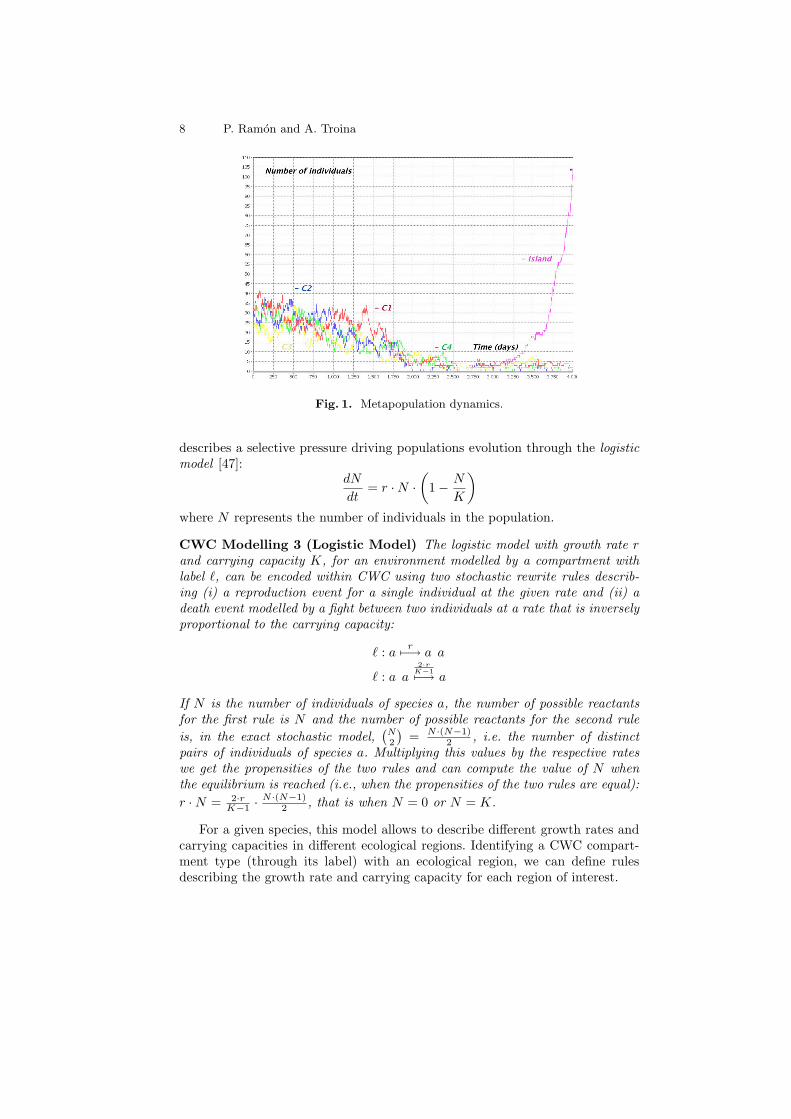
Example 1. Immigration and extinction are key components of island biogeogra-phy. We model a metapopulation of species a in a context of 5 different patches:4 of which are relatively close, e.g. different ecological regions within a smallcontinent, the last one is far away and difficult to reach, e.g. an island. Thecontinental patches are modelled as CWC compartments of type `c, the islandis modelled as a compartment of type ì. Births, deaths and migrations in thecontinental patches are modelled by the following CWC rules:

`c : a 0.0057−→ a a `c : a 0.0057−→ •> : (x c a X)`c 0.017−→ a (x cX)`c > : a (x cX)`c 0.57−→ (x c a X)`c

These rates are drawn considering days as time unites and an average of lifeexpectancy and reproduction time for the individuals of the species a of 200 days( 1

0.005 ). For the modelling of real case studies, these rates could be estimated fromdata collected in situ by tagging individuals.9 In this model, when an individualemigrates from its previous patch it moves to the top-level compartment fromwhere it may reach one of the close continental patches (might also be the oldone) or start a journey through the sea (modelled as a rewrite rule putting theindividual on the wrapping of the island compartment):

> : a (x cX)ì 0.27−→ (x a cX)ì

Crossing the ocean is a long and difficult task and individuals trying it willprobably die during the cruise; the luckiest ones, however, might actually reachthe island, where they could eventually benefit of a better life expectancy forthem and their descendants:

> : (x a cX)ì 0.3337−→ (x cX)ì > : (x a cX)ì 0.00057−→ (x c a X)ì

ì : a 0.0077−→ a a ì : a 0.0037−→ •

Considering the initial system modelled by the CWC term:

t = (• c 30 ∗ a)`c (• c 30 ∗ a)`c (• c 30 ∗ a)`c (• c 30 ∗ a)`c (• c •)ì

we can simulate the possible evolutions of the overall diffusion of individualsof species a in the different patches. Notice that, on average, one over 0.333

0.0005individuals that try the ocean journey, actually reach the island. In Figure 1 weshow the result of a simulation plotting the number of individuals in the differentpatches in a time range of approximatively 10 years. Note how, in the final partof the simulation, empty patches get recolonised. In this particular simulation,also, an exponential growth begins after the colonisation of the island. The fullCWC model describing this example can be found at: http://www.di.unito.it/~troina/cmc13/metapopulation.cwc.

In ecology, using r to represent the pro-capita growth rate of a population andK the carrying capacity of the hosting environment,10 r/K selection theory [38]9 In the remaining examples we will omit a detailed time description.

10 I.e., the population size at equilibrium.

http://www.di.unito.it/~troina/cmc13/metapopulation.cwc

http://www.di.unito.it/~troina/cmc13/metapopulation.cwc


Fig. 1. Metapopulation dynamics.

describes a selective pressure driving populations evolution through the logisticmodel [47]:

dN

dt= r ·N ·

(1− N

K

)where N represents the number of individuals in the population.

CWC Modelling 3 (Logistic Model) The logistic model with growth rate rand carrying capacity K, for an environment modelled by a compartment withlabel `, can be encoded within CWC using two stochastic rewrite rules describ-ing (i) a reproduction event for a single individual at the given rate and (ii) adeath event modelled by a fight between two individuals at a rate that is inverselyproportional to the carrying capacity:

` : a r7−→ a a

` : a a2·r

K−17−→ a

If N is the number of individuals of species a, the number of possible reactantsfor the first rule is N and the number of possible reactants for the second ruleis, in the exact stochastic model,

(N2

)= N ·(N−1)

2 , i.e. the number of distinctpairs of individuals of species a. Multiplying this values by the respective rateswe get the propensities of the two rules and can compute the value of N whenthe equilibrium is reached (i.e., when the propensities of the two rules are equal):r ·N = 2·r

K−1 ·N ·(N−1)

2 , that is when N = 0 or N = K.

For a given species, this model allows to describe different growth rates andcarrying capacities in different ecological regions. Identifying a CWC compart-ment type (through its label) with an ecological region, we can define rulesdescribing the growth rate and carrying capacity for each region of interest.


Species showing a high growth rate are selected by the r factor, they usuallyexploit low-crowded environments and produce many offspring, each of which hasa relatively low probability of surviving to adulthood. By contrast, K-selectedspecies adapt to densities close to the carrying capacity, tend to strongly competein high-crowded environments and produce fewer offspring, each of which has arelatively high probability of surviving to adulthood.

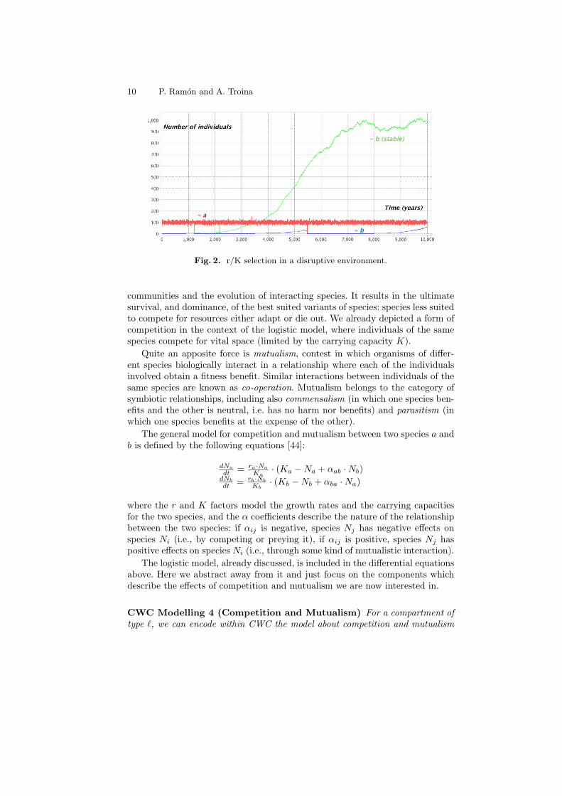
Example 2. There is little, or no advantage at all, in evolving traits that per-mit successful competition with other organisms in an environment that is verylikely to change rapidly, often in disruptive ways. Unstable environments thusfavour species that reproduce quickly (r-selected species). Stable environments,by contrast, favour the ability to compete successfully for limited resources (K-selected species). We consider individuals of two species, a and b. Individuals ofspecies a are modelled with an higher growth rate with respect to individuals ofspecies b (ra > rb). Carrying capacity for species a is, instead, lower than thecarrying capacity for species b (Ka < Kb). The following CWC rules describethe r/K selection model for ra = 5, rb = 0.00125, Ka = 100 and Kb = 1000:

` : a 57−→ a a ` : b 0.001257−→ b b

` : a a 0.17−→ a ` : b b 0.00000257−→ b

We might consider a disruptive event occurring on average every 4000 years withthe rule:

> : (x cX)` 0.000257−→ (x c a b)`

devastating the whole content of the compartment (modelled with the variableX) and just leaving one individual of each species. In Figure 2 we show a 10000years simulation for an initial system containing just one individual for eachspecies. Notice how individuals of species b are disadvantaged with respect toindividuals of species a who reach the carrying capacity very soon. A curveshowing the growth of individuals of species b in a stable (non disruptive) en-vironment is also shown. The full CWC model describing this example can befound at: http://www.di.unito.it/~troina/cmc13/rK.cwc.

3.2 Competition and Mutualism

In ecology, competition is a contest for resources between organisms: animals,e.g., compete for water supplies, food, mates, and other biological resources.In the long term period, competition among individuals of the same species(intraspecific competition) and among individuals of different species (interspe-cific competition) operates as a driving force of adaptation, and, eventually, bynatural selection, of evolution. Competition, reducing the fitness of the individ-uals involved,11 has a great potential in altering the structure of populations,11 By fitness it is intended the ability of surviving and reproducing. A reduction in

the fitness of an individual implies a reduction in the reproductive output. On theopposite side, a fitness benefit implies an improvement in the reproductive output.

http://www.di.unito.it/~troina/cmc13/rK.cwc


Fig. 2. r/K selection in a disruptive environment.

communities and the evolution of interacting species. It results in the ultimatesurvival, and dominance, of the best suited variants of species: species less suitedto compete for resources either adapt or die out. We already depicted a form ofcompetition in the context of the logistic model, where individuals of the samespecies compete for vital space (limited by the carrying capacity K).

Quite an apposite force is mutualism, contest in which organisms of differ-ent species biologically interact in a relationship where each of the individualsinvolved obtain a fitness benefit. Similar interactions between individuals of thesame species are known as co-operation. Mutualism belongs to the category ofsymbiotic relationships, including also commensalism (in which one species ben-efits and the other is neutral, i.e. has no harm nor benefits) and parasitism (inwhich one species benefits at the expense of the other).

The general model for competition and mutualism between two species a andb is defined by the following equations [44]:

dNa

dt = ra·Na

Ka· (Ka −Na + αab ·Nb)

dNb

dt = rb·Nb

Kb· (Kb −Nb + αba ·Na)

where the r and K factors model the growth rates and the carrying capacitiesfor the two species, and the α coefficients describe the nature of the relationshipbetween the two species: if αij is negative, species Nj has negative effects onspecies Ni (i.e., by competing or preying it), if αij is positive, species Nj haspositive effects on species Ni (i.e., through some kind of mutualistic interaction).

The logistic model, already discussed, is included in the differential equationsabove. Here we abstract away from it and just focus on the components whichdescribe the effects of competition and mutualism we are now interested in.

CWC Modelling 4 (Competition and Mutualism) For a compartment oftype `, we can encode within CWC the model about competition and mutualism


for individuals of two species a and b using the following stochastic rewrite rules:

` : a bfa·|αab|7−→

{a a b if αab > 0b if αab < 0 ` : a b

fb·|αba|7−→{a b b if αba > 0a if αba < 0

where fi = ri

Kiis obtained from the usual growth rate and carrying capacity. The

α coefficients are put in absolute value to compute the rate of the rule, their signsaffect the right hand part of the rewrite rule.

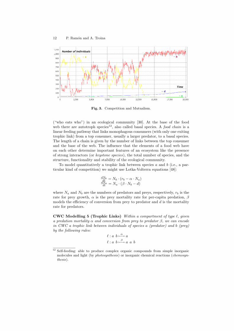
Example 3. Mutualism has driven the evolution of much of the biological di-versity we see today, such as flower forms (important to attract mutualisticpollinators) and co-evolution between groups of species [45]. We consider twodifferent species of pollinators, a and b, and two different species of angiosperms(flowering plants), c and d. The two pollinators compete between each other, andso do the angiosperms. Both species of pollinators have a mutualistic relationwith both angiosperms, even if a slightly prefers c and b slightly prefers d. Foreach of the species involved we consider the rules for the logistic model and foreach pair of species we consider the rules for competition and mutualism. Theparameters used for this model are in Table 1. So, for example, the mutualisticrelations between a and c are expressed by the following CWC rules

> : a craKa·αac

7−→ a a c > : a crcKc·αca

7−→ a c c

Figure 3 shows a simulation obtained starting from a system with 100 individ-uals of species a and b and 20 individuals of species c and d. Note the initiallybalanced competition between pollinators a and b. This random fluctuations areresolved by the “long run” competition between the angiosperms c and d: when dpredominates over c it starts favouring the pollinator b that now can win its owncompetition with pollinator a. The model is completely symmetrical: in otherruns, a faster casual predominance of a pollinator may lead the evolution of itspreferred angiosperm. The CWC model describing this example can be foundat: http://www.di.unito.it/~troina/cmc13/compmutu.cwc.

Species (i) ri Ki αai αbi αci αdi

a 0.2 1000 • -1 +0.03 +0.01

b 0.2 1000 -1 • +0.01 +0.03

c 0.0002 200 +0.25 +0.1 • -6

d 0.0002 200 +0.1 +0.25 -6 •Table 1. Parameters for the model of competition and mutualism.

3.3 Trophic Networks

A food web is a network mapping different species according to their alimentaryhabits. The edges of the network, called trophic links, depict the feeding pathways

http://www.di.unito.it/~troina/cmc13/compmutu.cwc


Fig. 3. Competition and Mutualism.

(“who eats who”) in an ecological community [30]. At the base of the foodweb there are autotroph species12, also called basal species. A food chain is alinear feeding pathway that links monophagous consumers (with only one exitingtrophic link) from a top consumer, usually a larger predator, to a basal species.The length of a chain is given by the number of links between the top consumerand the base of the web. The influence that the elements of a food web haveon each other determine important features of an ecosystem like the presenceof strong interactors (or keystone species), the total number of species, and thestructure, functionality and stability of the ecological community.

To model quantitatively a trophic link between species a and b (i.e., a par-ticular kind of competition) we might use Lotka-Volterra equations [48]:

dNb

dt = Nb · (rb − α ·Na)dNa

dt = Na · (β ·Nb − d)

where Na and Nb are the numbers of predators and preys, respectively, rb is therate for prey growth, α is the prey mortality rate for per-capita predation, βmodels the efficiency of conversion from prey to predator and d is the mortalityrate for predators.

CWC Modelling 5 (Trophic Links) Within a compartment of type `, givena predation mortality α and conversion from prey to predator β, we can encodein CWC a trophic link between individuals of species a (predator) and b (prey)by the following rules:

` : a b α7−→ a

` : a bβ7−→ a a b

12 Self-feeding: able to produce complex organic compounds from simple inorganicmolecules and light (by photosynthesis) or inorganic chemical reactions (chemosyn-thesis).


Here we omitted the rules for the prey exponential growth (absent predators)and predators exponential death (absent preys). These factors are present in theLotka-Volterra model between two species, but could be substituted by the effectsof other trophic links within the food web. In a more general scenario, a trophiclink between species a and b could be expressed condensing the two rules withinthe single rule:

` : a bγ7−→ a a

with a rate γ modelling both the prey mortality rate and the predator conversionfactor.

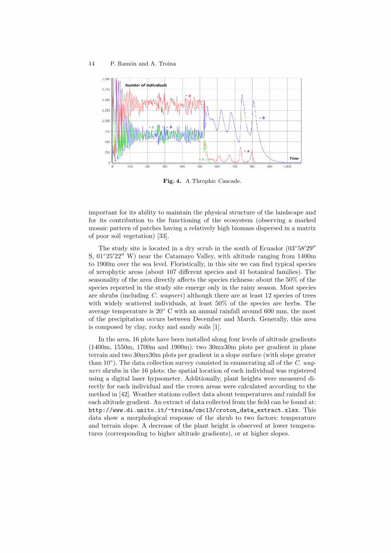
Example 4. Trophic cascades occur when predators in a food web suppress theabundance of their prey, thus limiting the predation of the next lower trophiclevel. For example, an herbivore species could be considered in an intermediatetrophic level between a basal species and an higher predator. Trophic cascadesare important for understanding the effects of removing top predators from foodwebs, as humans have done in many ecosystems through hunting or fishing ac-tivities. We consider a three-level food chain between species a, b and c. Thebasal species a reproduces with the logistic model, the intermediate species bfeeds on a, species c predates species b:

` : a0.47−→ a a ` : a a

0.00027−→ a ` : a b0.00047−→ b b ` : b c

0.00087−→ c c

Individuals of species c die naturally, until an hunting species enters the ecosys-tem. At a rate lower than predation, b may also die naturally (absent predator).An atom h may enter the ecosystem and start hunting individuals of species c:

` : c0.527−→ • ` : b

0.037−→ • > : h (x cX)` 0.0037−→ (x cX h)` ` : h c0.57−→ h

Figure 4 shows a simulation for the initial term h (• c 1000 ∗ a 100 ∗ b 10 ∗ c)`.When the hunting activity starts, by removing the top predator, a top-downcascade destroys the whole community. The CWC model describing this examplecan be found at: http://www.di.unito.it/~troina/cmc13/trophic.cwc.

4 An application: Croton wagneri and Climate Change

Dry ecosystems are characterised by the presence of discontinuous vegetationthat may reflect less than 60% of the available landscape. The main patternin arid ecosystems is a vegetation mosaic composed of patches and clear sites.In [31] about 1300 different species belonging to the dry ecosystems in NorthwestSouth America have been identified.

For this study we focused on the species Croton wagneri Mull. Arg., belongingto the Euphorbiaceae family. This species, particularly widespread in tropicalregions, can be identified by the combination of latex, alternate simple leaves, apair of glands at the apex of the petiole, and the presence of stipules. C. wagneriis the dominant endemic shrub in the dry scrub of Ecuador and has been listedas Near Threatened (NT) in the Red Book of Endemic Plants of Ecuador [46].This kind of shrub could be considered as a nurse species13 and is particularly13 A nurse plant is one with an established canopy, beneath which germination and

survival are more likely due to increased shade, soil moisture, and nutrients.

http://www.di.unito.it/~troina/cmc13/trophic.cwc


Fig. 4. A Throphic Cascade.

important for its ability to maintain the physical structure of the landscape andfor its contribution to the functioning of the ecosystem (observing a markedmosaic pattern of patches having a relatively high biomass dispersed in a matrixof poor soil vegetation) [33].

The study site is located in a dry scrub in the south of Ecuador (03◦58′29′′

S, 01◦25′22′′ W) near the Catamayo Valley, with altitude ranging from 1400mto 1900m over the sea level. Floristically, in this site we can find typical speciesof xerophytic areas (about 107 different species and 41 botanical families). Theseasonality of the area directly affects the species richness: about the 50% of thespecies reported in the study site emerge only in the rainy season. Most speciesare shrubs (including C. wagneri) although there are at least 12 species of treeswith widely scattered individuals, at least 50% of the species are herbs. Theaverage temperature is 20◦ C with an annual rainfall around 600 mm, the mostof the precipitation occurs between December and March. Generally, this areais composed by clay, rocky and sandy soils [1].

In the area, 16 plots have been installed along four levels of altitude gradients(1400m, 1550m, 1700m and 1900m): two 30mx30m plots per gradient in planeterrain and two 30mx30m plots per gradient in a slope surface (with slope greaterthan 10◦). The data collection survey consisted in enumerating all of the C. wag-neri shrubs in the 16 plots: the spatial location of each individual was registeredusing a digital laser hypsometer. Additionally, plant heights were measured di-rectly for each individual and the crown areas were calculated according to themethod in [42]. Weather stations collect data about temperatures and rainfall foreach altitude gradient. An extract of data collected from the field can be found at:http://www.di.unito.it/~troina/cmc13/croton_data_extract.xlsx. Thisdata show a morphological response of the shrub to two factors: temperatureand terrain slope. A decrease of the plant height is observed at lower tempera-tures (corresponding to higher altitude gradients), or at higher slopes.

http://www.di.unito.it/~troina/cmc13/croton_data_extract.xlsx


4.1 The CWC model

A simulation plot is modelled by a compartment with label P . Atoms g, repre-senting the plot gradient (one g for each metre of altitude over the level of thesea), describe an abiotic factor put in the compartment wrap.

According to the temperature data collected by the weather stations we corre-late the mean temperatures in the different plots with their respective gradients.In the content of a simulation plot, atoms t, representing 1◦C each, model itstemperature. Remember that, in this case, the higher the gradient, the lowerthe temperature. Thus, we model a constant increase of temperature within thesimulation plot compartment, controlled by the gradient elements g on its wrap:

> : (x cX)P 17−→ (x c t X)P > : (g x c t X)P 0.0000247−→ (g x cX)P

Atoms i are also contained within compartments of type P , representing thecomplementary angle of the plot’s slope (e.g., 90 ∗ i for a plane plot or 66 ∗ i fora 24◦ slope).

We model C. wagneri as a CWC compartment with label c. Its observedtrait, namely the plant height, is specified by atomic elements h (representingone mm each) on the compartment wrap.

To model the shrub heights distribution within a parcel, we consider theplant in two different states: a “young” and an “adult” state. Atomic elementsy and a are exclusively, and uniquely, present within the plant compartment insuch a way that the shrub height increases only when the shrub is in the youngstate (y in its content). The following rules describe (i) the passage of the plantfrom y to a state with a rate corresponding to a 1 year average value, and (ii) thegrowth of the plant, affected by temperature and slope, with a rate estimatedto fit the field collected data:

c : y 0.002747−→ a P : t i (x c y X)c 0.0007187−→ t i (x h c y X)c

4.2 Simulation results

Now we have a model to describe the distribution of C. wagneri height usingas parameters the plot’s gradient (n ∗ g) and slope (m ∗ i). Since we do notmodel explicitly interactions that might occur between C. wagneri individuals,we consider plots containing a single shrub. Carrying on multiple simulations,through the two phase model of the plant growth, after 1500 time units (hererepresented as days), we get a snapshot of the distribution of the shrubs heightswithin a parcel. The CWC model describing this application can be found at:http://www.di.unito.it/~troina/cmc13/croton.cwc.

Each of the graphs in Figure 5 is obtained by plotting the height deviationof 100 simulations with initial term (n ∗ g cm ∗ i (• c y)c)P . The simulations inFigures 5 (a) and (c) reflect the conditions of real plots and the results give agood approximation of the real distribution of plant heights. Figures 5 (b) and(d) are produced considering an higher slope than the ones on the real plots

http://www.di.unito.it/~troina/cmc13/croton.cwc


from were the data has been collected. These simulation results can be used forfurther validation of the model by collecting data on new plots corresponding tothe parameters of the simulation.

(a) 1400 ∗ g and 90 ∗ i (b) 1550 ∗ g and 60 ∗ i

(c) 1700 ∗ g and 85 ∗ i (d) 1900 ∗ g and 75 ∗ i

Fig. 5. Deviation of the height of Croton wagneri for 100 simulations.

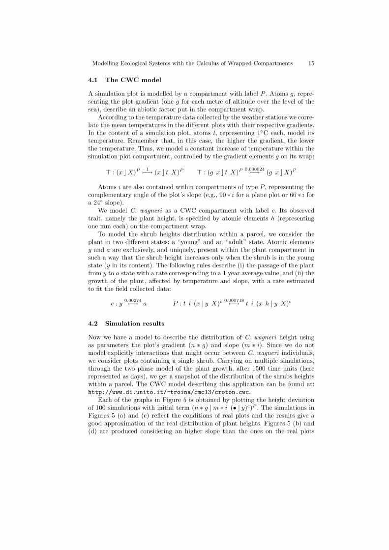
If we already trust the validity of our model, we can remove the correla-tion between the gradient and the temperature, and directly express the latter.Predictions can thus be made about the shrub height at different temperatures,and how it could adapt to global climate change. Figure 6 shows two possibledistributions of the shrub height at lower temperatures (given it will actuallysurvive these more extreme conditions and follow the same trend).

5 Conclusions and Related Works

The long-term goal of Computational Ecology is the development of methods topredict the response of ecosystems to changes in their physical, chemical and bio-logical components. Computational models, and their ability to understand andpredict the biological world, could be used to express the mechanisms governingthe structure and function of natural populations, communities, and ecosystems.Until recent times, there was insufficient computational power to run stochas-


(a) 12◦C, plain terrain (b) 10◦C, plain terrain

Fig. 6. Deviation of the height of Croton wagneri for 100 simulations.

tic, individually-based, spatially explicit models. Today, however, some of thesetechniques could be investigated [37].

Calculi developed to describe process interactions in a compartmentalisedsetting are well suited for the description and analysis of the evolution of eco-logical systems. The topology of the ecosystem can be directly encoded withinthe nested structure of the compartments. These calculi can be used to repre-sent structured natural processes in a greater detail, when compared to purelynumerical analysis. As an example, food webs can give rise to combinatorialinteractions resulting in the formation of complex systems with emergent prop-erties (as signalling pathways do in cellular biology), and, in some cases, givingrise to chaotic behaviour.

As a final remark about ecological modelling with a framework based onstochastic rewrite rules, we underline an important compositional feature. Howcan we test an hypothetical scenario where a grazing species is introduced in themodel of our case study? A possibility could be to represent the grazing specieswith a new CWC atom (e.g. s) and then just add the new competitive rules tothe previously validated model (e.g. the rule P : s (h x cX)c 7−→ s (x cX)c).Changing in the same sense a model based on ordinary differential equationswould, instead, result in a complete new model were all previous equations shouldbe rewritten.

5.1 Related works

As P-Systems [40,41] and the Calculus of Looping Sequences (CLS, for short) [11],the Calculus of Wrapped Compartments is a framework modelling topologicalcompartmentalisation inspired by biological membranes, and with a semanticsgiven in terms of rewrite rules.

CWC has been developed as a simplification of CLS, focusing on stochasticmultiset rewriting. The main difference between CWC and CLS consists in theexclusion of the sequence operator, that constructs ordered strings out of theatomic elements of the calculus. While the two calculi keep the same expres-siveness, some differences arise on the way systems are described. On the one


hand, the Calculus of Looping Sequences allows to define ordered sequences ina more succinct way (for examples when describing sequences of genes in DNAor sequences of amino acids in proteins).14 On the other hand, CWC reflectsin a more realistic way the fluid mosaic model of the lipid bilayer (for examplein the case of cellular membrane description, where proteins are free to float),and, the addition of compartment labels allows to characterise the propertiespeculiar to given classes of compartments. Ultimately, focusing on multisets andavoiding to deal explicitly with ordered sequences (and, thus, variables for se-quences) strongly simplifies the pattern matching procedure in the developmentof a simulation tool.

The Calculus of Looping Sequences has been extended with type systemsin [6,28,29,8,16]. As an application to ecology, stochastic CLS (see [7]) is usedin [12] to model population dynamics.

P-Systems have been proposed as a computational model inspired by biolog-ical structures. They are defined as a nesting of membranes in which multisets ofobjects can react according to pre defined rewrite rules. Maximal-parallelism isthe key feature of P-Systems: at each evolution step all rewrite rules, in all mem-branes, are applied as many times as possible. Such a feature makes P-Systemsa very powerful computational model and a versatile instrument to evaluateexpressiveness of languages. However, it is not practical to describe stochasticsystems with a maximally-parallel evolution: exact stochastic simulations basedon race conditions model systems evolutions as a sequence of successive steps,each of which with a particular duration modelled by an exponential probabilitydistribution.

There is a large body of literature about applications of P-Systems to ecolog-ical modelling. In [20,21,22], P-Systems are enriched with a probabilistic seman-tics to model different ecological systems in the Catalan Pyrenees. Rules couldstill be applied in a parallel fashion since reduction durations are not explic-itly taken into account. In [13,14,15], P-Systems are enriched with a stochasticsemantics and used to model metapopulation dynamics. The addition of muterules allows to keep a form of parallelism reducing the maximal consumption ofobjects.

While all these calculi allow to manage systems topology through nestingand compartmentalisation, explicit spatial models are able to depict more preciselocalities and ecological niches, describing how organisms or populations respondto the distribution of resources and competitors [35]. The spatial extensions ofCWC [17], CLS [9] and P-Systems [10] could be used to express this kind ofanalysis allowing to deal with spatial coordinates.

References

1. Aguirre, Z., Kvist, P., Sanchez, O.: Floristic composition and conservation statusof the dry forests in ecuador. Lyonia 8(2) (2005)

14 An ordered sequence can be expressed in CWC as a series of nested compartments,ordered from the outermost compartment to the innermost one.


2. Aldinucci, M., Coppo, M., Damiani, F., Drocco, M., Giovannetti, E., Grassi, E.,Sciacca, E., Spinella, S., Troina, A.: CWC Simulator. Dipartimento di Informatica,Universita di Torino (2010), http://cwcsimulator.sourceforge.net/

3. Aldinucci, M., Coppo, M., Damiani, F., Drocco, M., Sciacca, E., Spinella, S.,Torquati, M., Troina, A.: On parallelizing on-line statistics for stochastic biologicalsimulations. In: HiBB’11. Lecture Notes in Computer Science, vol. 7156, pp. 3–12.Springer (2011)

4. Aldinucci, M., Coppo, M., Damiani, F., Drocco, M., Torquati, M., Troina, A.:On designing multicore-aware simulators for biological systems. In: Proc. of Intl.Euromicro PDP 2011: Parallel Distributed and network-based Processing. pp. 318–325. IEEE Computer Society (2011)

5. Aldinucci, M., Torquati, M.: FastFlow website. FastFlow (Oct 2009), http://

mc-fastflow.sourceforge.net/6. Aman, B., Dezani-Ciancaglini, M., Troina, A.: Type disciplines for analysing bio-

logically relevant properties. Electr. Notes Theor. Comput. Sci. 227, 97–111 (2009)7. Barbuti, R., Maggiolo-Schettini, A., Milazzo, P., Tiberi, P., Troina, A.: Stochastic

calculus of looping sequences for the modelling and simulation of cellular pathways.Transactions on Computational Systems Biology IX, 86–113 (2008)

8. Barbuti, R., Dezani-Ciancaglini, M., Maggiolo-Schettini, A., Milazzo, P., Troina,A.: A formalism for the description of protein interaction. Fundam. Inform. 103(1-4), 1–29 (2010)

9. Barbuti, R., Maggiolo-Schettini, A., Milazzo, P., Pardini, G.: Spatial calculus oflooping sequences. Theoretical Computer Science 412(43), 5976 – 6001 (2011)

10. Barbuti, R., Maggiolo-Schettini, A., Milazzo, P., Pardini, G., Tesei, L.: Spatial psystems. Natural Computing 10(1), 3–16 (2011)

11. Barbuti, R., Maggiolo-Schettini, A., Milazzo, P., Troina, A.: The calculus of loopingsequences for modeling biological membranes. In: Workshop on Membrane Com-puting. Lecture Notes in Computer Science, vol. 4860, pp. 54–76. Springer (2007)

12. Basuki, T.A., Cerone, A., Barbuti, R., Maggiolo-Schettini, A., Milazzo, P., Rossi,E.: Modelling the dynamics of an aedes albopictus population. In: AMCA-POP.vol. 33, pp. 18–36. EPTCS (2010)

13. Besozzi, D., Cazzaniga, P., Pescini, D., Mauri, G.: Seasonal variance in p systemmodels for metapopulations. Progress in Natural Science 17(4), 392–400 (2007)

14. Besozzi, D., Cazzaniga, P., Pescini, D., Mauri, G.: Modelling metapopulations withstochastic membrane systems. Biosystems 91(3), 499–514 (2008)

15. Besozzi, D., Cazzaniga, P., Pescini, D., Mauri, G.: An analysis on the influence ofnetwork topologies on local and global dynamics of metapopulation systems. In:AMCA-POP. vol. 33, pp. 1–17. EPTCS (2010)

16. Bioglio, L., Dezani-Ciancaglini, M., Giannini, P., Troina, A.: Typed stochasticsemantics for the calculus of looping sequences. Theor. Comp. Sci. 431, 165–180

17. Bioglio, L., Calcagno, C., Coppo, M., Damiani, F., Sciacca, E., Spinella, S., Troina,A.: A spatial calculus of wrapped compartments. In: MeCBIC. vol. abs/1108.3426.CoRR (2011)

18. Bolker, B.: Ecological models and data in R. Princeton University Press (2008)19. Calcagno, C., Coppo, M., Damiani, F., Drocco, M., Sciacca, E., Spinella, S., Troina,

A.: Modelling spatial interactions in the arbuscular mycorrhizal symbiosis using thecalculus of wrapped compartments. In: CompMod 2011. vol. 67, pp. 3–18. EPTCS(2011)

20. Cardona, M., Colomer, M.A., Margalida, A., Palau, A., Perez-Hurtado, I., Perez-Jimenez, M.J., Sanuy, D.: A computational modeling for real ecosystems based onp systems. Natural Computing 10(1), 39–53 (2011)

http://cwcsimulator.sourceforge.net/

http://mc-fastflow.sourceforge.net/

http://mc-fastflow.sourceforge.net/


21. Cardona, M., Colomer, M.A., Margalida, A., Perez-Hurtado, I., Perez-Jimenez,M.J., Sanuy, D.: A p system based model of an ecosystem of some scavenger birds.In: 10th Workshop on Membrane Computing. Lecture Notes in Computer Science,vol. 5957, pp. 182–195. Springer (2010)

22. Cardona, M., Colomer, M.A., Perez-Jimenez, M.J., Sanuy, D., Margalida, A.: Mod-eling ecosystems using p systems: The bearded vulture, a case study. In: MembraneComputing, pp. 137–156. Springer (2009)

23. Caswell, H.: Matrix population models: Construction, analysis and interpretation,2nd Edition. Sinauer Associates, Sunderland, Massachusetts. (2001)

24. Coppo, M., Damiani, F., Drocco, M., Grassi, E., Guether, M., Troina, A.: Mod-elling ammonium transporters in arbuscular mycorrhiza symbiosis. Transactionson Computational Systems Biology XIII, 85–109 (2011)

25. Coppo, M., Damiani, F., Drocco, M., Grassi, E., Sciacca, E., Spinella, S., Troina,A.: Simulation techniques for the calculus of wrapped compartments. Theor. Comp.Sci. 431, 75–95

26. Coppo, M., Damiani, F., Drocco, M., Grassi, E., Sciacca, E., Spinella, S., Troina,A.: Hybrid calculus of wrapped compartments. In: MeCBIC. vol. 40, pp. 103–121.EPTCS (2010)

27. Coppo, M., Damiani, F., Drocco, M., Grassi, E., Troina, A.: Stochastic Calculusof Wrapped Compartments. In: QAPL. vol. 28, pp. 82–98. EPTCS (2010)

28. Dezani-Ciancaglini, M., Giannini, P., Troina, A.: A type system for re-quired/excluded elements in CLS. In: DCM’09. vol. 9, pp. 38–48. EPTCS (2009)

29. Dezani-Ciancaglini, M., Giannini, P., Troina, A.: A type system for a stochasticcls. In: MeCBIC’09. vol. 11, pp. 91–105. EPTCS (2009)

30. Elton, C.: Animal Ecology. Sidgwick and Jackson (1927)31. Gentry, A.: A Field Guide to the Families and Genera of Woody Plants of North-

west South America: (Colombia, Ecuador, Peru): with supplementary notes onherbaceous taxa. Washington DC, Conservation International (1993)

32. Gillespie, D.: Exact stochastic simulation of coupled chemical reactions. J. Phys.Chem. 81, 2340–2361 (1977)

33. Gutierrez, J.: Importancia de los Arbustos Lenosos en los Ecosistemas de la IVRegion, Libro Rojo de la Flora Nativa y de los Sitios Prioritarios para su Conser-vacion: Region de Coquimbo, vol. 16. Ediciones Universidad de La Serena, Chile(2001)

34. Levins, R.: Some demographic and genetic consequences of environmental hetero-geneity for biological control. Bulletin of the Entomological Society of America 15,237–240 (1969)

35. Lomolino, M.V., Brown, J.W.: Biogeography. Sunderland, Mass: Sinauer Asso-ciates. (1998)

36. Oury, N., Plotkin, G.: Multi-level modelling via stochastic multi-level multisetrewriting. Mathematical Structures in Computer Science (2012)

37. Petrovskii, S., Petrovskaya, N.: Computational ecology as an emerging science.Interface Focus 2(2), 241–254 (2012)

38. Pianka, E.: On r and k selection. American Naturalist 104(940), 592–597 (1970)39. Pielou, E.: Mathematical ecology. Wiley (1977)40. Paun, G.: Computing with membranes. Journal of Computer and System Sciences

61(1), 108–143 (2000)41. Paun, G.: Membrane Computing. An Introduction. Springer (2002)42. Shiponeni, N., Allsopp, N., Carrick, P., Hoffman, M.: Competitive interactions

between grass and succulent shrubs at the ecotone between an arid grassland andsucculent shrubland in the karoo. Plant. Ecol. 212(5), 795–808 (2011)


43. Sugihara, G., May, R.: Nonlinear forecasting as a way of distinguishing chaos frommeasurement error in time series. Nature 344(6268), 734–741 (1990)

44. Takeuchi, Y.: Cooperative systems theory and global stability of diffusion models.Acta Applicandae Mathematicae 14, 49–57 (1989)

45. Thompson, J.: The geographic mosaic of coevolution. University of Chicago Press(2005)

46. Valencia, R., Pitman, N., Leon-Yanez, S., Jorgensen, P.: Libro Rojo de las Plan-tas Endemicas del Ecuador. Herbario QCA, Pontificia Universidad Catolica delEcuador, Quito (2000)

47. Verhulst, P.: Notice sur la loi que la population pursuit dans son accroissement.Corresp. Math. Phys. 10, 113–121 (1838)

48. Volterra, V.: Variazioni e fluttuazioni del numero dindividui in specie animali con-viventi. Mem. Acad. Lincei Roma 2, 31–113 (1926)

modelling ecological systems with the calculus of wrapped ... filemodelling ecological systems with...

Documents