Modelling environmental systems

Some words on modelling

the hitchhiker’s guide to modelling

Problem perception

• Definition of the scope of the model

• Clearly define your objectives

• Allow for incremental model definition (don’t start with a model which is too complex)

• Work in strict co-operation with the Decision Makers

Limits to modelling

• We tend to think linear

• System structure influences behaviour

• Structure in human system is subtle

• Leverage often comes from new ways of thinking

• Reductionist thinking is often hampering

Systems thinking• for seeing wholes, counteract reductionism

• relationships rather than things

• patterns of change rather than static snapshots

• seeing circles of causality

• dealing with complexity and delays

• acknowledging both hard and soft components

What is a model?• A model is any understanding which is used

to reach a conclusion or a solution

• Only mental models exist; all models rest in the human mind

• There are no computer models, these are mere mechanical and mathematical pictures of mental models

• If a model is ”wrong”, then the underlying understanding is to blame

Modelling: the hardest part

Sorting the essential from the nonessentials!

Needed Unnecessary

• how useful it is for it’s purpose

• how well users understand the model and have trust in it

• NOT the number of details

The quality of a model is determined by

Simplicity and participation

• The major result is understanding (not the models themselves)

• Simple models ensure understanding

• Modelling is not a one man work!

• The process is everything! (”The road is the goal”)

One question – one model!

Never trust a Swiss Army knife model!

Model categories and classification

Breeds of models

• Models are

• conceptual

• physical

• mathematical

Models aremental/

conceptualphysical mathematical

system identification encompasses..

definition of system boundary, components, interactions

The model is...a conceptual, verbal

description of system behaviour

a scaled reproduction of a

real system

coupling of functions, rules,

equations

Elements of a model are..

premises, conclusions, syllogisms

a physical objectmathematical

functions and (state) variables

Plausibility check is..conclusions are

tested on real-world cases

an experiment in a controlled

environment

validation and sensitivity analyses

A simulation is..a thinking

experimenta physical

experimenta numerical solution of the equation sets

(adapted from Seppelt, 2003)

Temporal scale

• Defined by the “time constant” τ of the system

• In relation with the integration step ∆t

• τ=1/∆t

• Choice of the temporal scale and “stiff” systems

Process VariablesCharacteristic

timeMathematical

model

Microbial growthBiomass, nitrogen

content30 minutes ODE

Nitrification, denitrification

Nitrogen compoundes,

micrrobial activity1 day to 1 week Systems of ODE

Population dynamicsDensity of eggs, juveniles, larvae,

adultsWeeks

DAE, DDE, Systems of ODE

Crop growthBiomass, nitrogen content, leaf area

indexMonth Systems of ODE

Water transport in unsaturated soil

Water content 1 hour PDE

Solute transport in aquifers

Concentration in liquid and solute

phase

large up to several years

PDE coupled with ODE system

(Seppelt, 2003)

Spatial scale

• It is the spatial extent

• how many dimensions?

• what is the grid size?

Model use

• Descriptive models

• Decision models

• Prescriptive models

• Forecast models

Conceptual models

A conceptual model

• is presented graphically as a compartment system

• compartments are defined w.r.t morphology, and physical, chemical and biological states

• connections denote exchange of matter, energy, information

• compartments may contain sub-models

Types of conceptual models

• Word models

• Picture models

• Box-models

• Feedback dynamics, Casual Loop Diagrams

• Energy Circuit Diagrams (Odum)

!"#$#%&'($)*$+,%-

.$)$/%#%)-

012345#'6345#*74-

.)75%--%-

6,78-

974#)7,'($)*$+,%-

:7341$);'9741*#*74-

67)5*4<'6345#*74-

:7='>71%,- 6%%1+$5?'

@;4$/*5-

A4%)<;'

6,78'

>71%,-

"#$#%'($)

B$#%

974-#$4#C

6345#*74

"*4?D"73)5%

"#$#%($)

974-#$4#

6345#*74

6,78

AE%4#

AE%4#

F4G3#H

I3#G3#

>71%,-

B$#%

"#$#%

.%#)*'J%#-

.,$5%

6,78

K)$4-*#*74

F4#%)$5#*74

A=5L$4<%'7M'

F4M7)/$#*74

"3+H";-#%/-

"73)5%

"*4?

K)$4-$5#*74

974-3/%)

"#7)$<%

0/G,*M;%)

9;5,*4<'B%5%G#7)

Paradigms for

Conceptual Modelling

(Seppelt, 2003)

Causal loop diagramsFeedback dynamics

What is a Causal Loop Diagram?

• A simplified understanding of a complex problem

• A common language to convey the understanding

• A way of explaining cause and effect relationships

• Explanation of underlying feedback systems

• Helps us understanding the overall system behaviour

Reinforcing feedback

• Reinforcing behaviour

• Something that causes an amplified condition

• the larger the population the more births

• the more money in the bank, the more in interest

R

Balancing feedback

• Balancing behaviour

• Something that causes a change which dampens/opposes a condition,

• Limited amounts of nutrients

• Intensity of competition

B

Reinforcing

• A self-reinforcing system is a system in growth, e.g. bank account, economic growth or population growth, exponential growth

An example of system in growth over time

2001 2002 2003 20040

25

50

75

100

time

quan

tity

Balancing

• In a balancing system there is an agent which retards the growth or is a limiting factor to the reinforcing growth, e.g. limited resources in the soil, limited light or space for growth etc.

An example of system that balances over time

2001 2002 2003 20040

25

50

75

100

time

quan

tity

The structure of CausalityVariables change:

”in the same direction”

”in the opposite direction”

A very simple example

Photosynthesis Growth

+

+

R

Another simple example

Nutrientuptake

Nutrientsavailable

-

+

B

a bit more complex

Some practice with CLD

Atmospheric system

Natural system

Social system

Economic system

Combined system

The difficult transition from conceptual to

mathematical models

Problem formulation

• Conceptual model construction

• System boundaries

• CLD

• Actors, Drivers and Conditions

• Reference behaviour

Model construction

• From conceptual model to quantitative model

• Parameterization

• Sensitivity and robustness testing

• Model validation

The modelling processScope/

Purpose

Conceptualisation

Calibration

Validation

Use

Data collection

Problems in conceptual modelling

• What is relevant? Sorting out essentials

• At what level? Micro- or Macro-level

• Static and dynamic factors?

• System boundaries?

• Time horizon

• Qualitative and/or quantitative factors?

• Problems to ”kill your darlings”

• Perception limitations

Conceptual model building factors

• Deletion

• Select and filter according to preferences, mode, mood, interest, preoccupation and congruency

• Construction

• See something that is not there, filling in gaps

• Distortion

• Amplifying some parts and diminishing others, reading different meanings into it

Conceptual model building factors

• Generalisation

• One experience comes to represent a whole class of experiences

• One-sided experiences

• We tend to only remember one side of experiences

Problems in the CLD to model phase

• Including how many components?

• How to distinguish accumulations from processes?

• Units?

• Scales?

• Introduction of mass and energy balance principles?

• Non-linear relationships

• Qualitative components

Problems in the model validation phase

• Finding data for validation

• Robustness of model

• Qualitative components

• Appropriate time and space boundaries

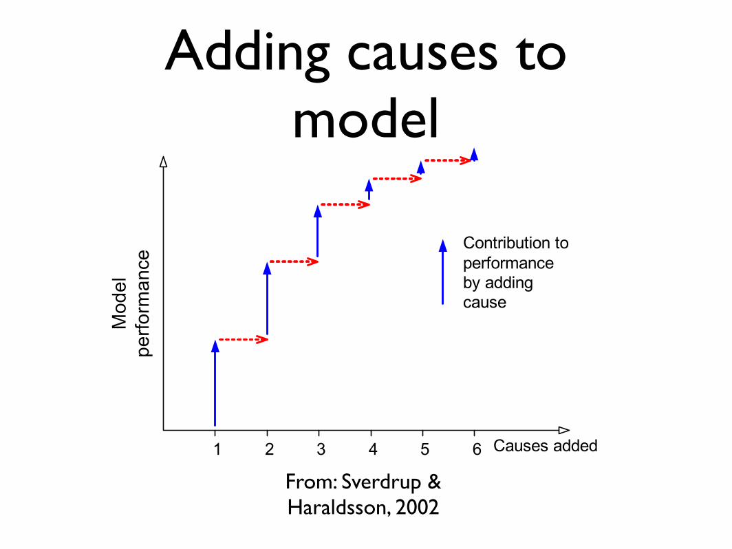
Adding causes to model

From: Sverdrup & Haraldsson, 2002

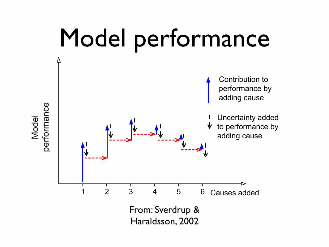
Model performance

From: Sverdrup & Haraldsson, 2002

Model cost and performance

From: Sverdrup & Haraldsson, 2002

System Levels

From: Sverdrup & Haraldsson, 2002

Mathematical models

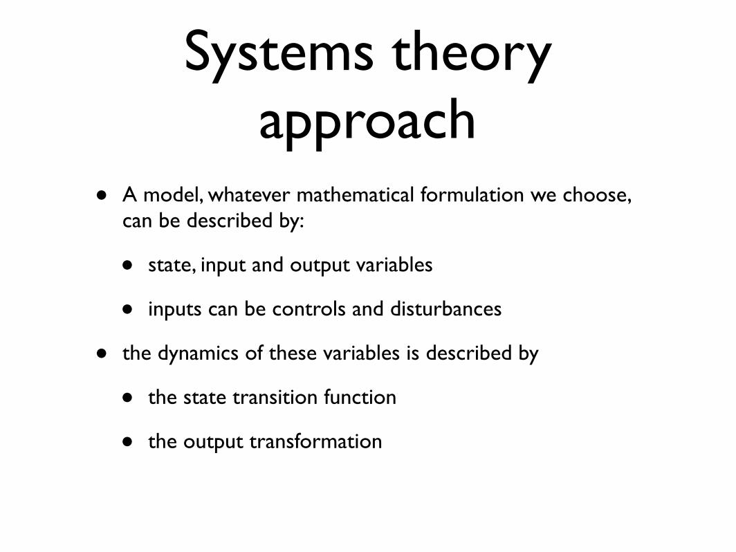
Systems theory approach

• A model, whatever mathematical formulation we choose, can be described by:

• state, input and output variables

• inputs can be controls and disturbances

• the dynamics of these variables is described by

• the state transition function

• the output transformation

The equations

xt+!t(z) =M!t(xt(z),ut(z),"(z),z)

General model equation

x0(z)Initial condition

and boundary conditions

yt(z) = ft(xt(z))

Dynamic vs static

• A dynamic system needs to store information in the state to evolve

• If the state at time t-1 is sufficient to compute the state at time t, then the system is Markovian

• If a system can be described only by its output transformation is static

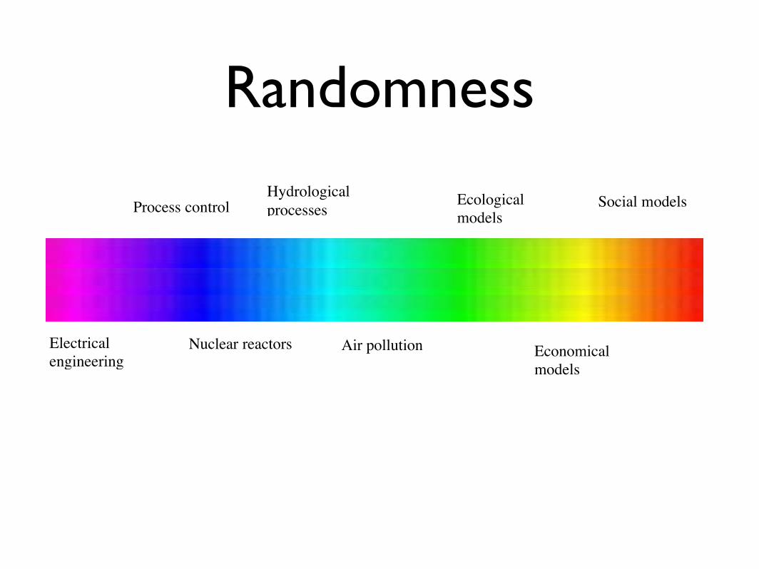
Randomness

Process controlHydrologicalprocesses

Electricalengineering

Nuclear reactors Air pollution

Ecologicalmodels

Social models

Economicalmodels

Model paradigms

• Scarce theoretical modelling knowledge, many data: Bayesian Belief Networks

• Good theoretical knowledge: mechanistic models

• Very little knowledge: empirical models

• Mixed knowledge: Data Based Mechanistic models

Mechanistic Models

• Ordinary Differential Equations

• Difference Equations

• Partial Differential Equations

• Stochastic models

Empirical Models

• Completely data-driven

• No insight on the model causal structure

• Input-output models

• Neural Networks

yt+1 = yt(yt , . . . ,yt−(p−1),ut+1, . . . ,ut−(r′−1),wt+1, . . . . . . ,wt−(r′′−1),!t+1, . . . ,!t−(q−1)

). . . ,wt−(r′′−1),!t+1, . . . ,!t−(q−1)

Data Based Mechanistic models

• Mechanistic models are too complex and require too many details

• Empirical model use a-priori classes

• A new approach to model identification

• Input/Output relationships are extracted from data

• Proposed by Young and Beven, 1994

An input-output model fails

01.02.85 11.05.85 19.08.85 27.11.85 07.03.86 15.06.86 24.09.86 02.01.870

1

2

3

4

Deflusso

01.02.85 11.05.85 19.08.85 27.11.85 07.03.86 15.06.86 24.09.86 02.01.870

20

40

60

80

Precipitazione

yt+1 = !yt +"wt + #t+1

01.02.85 11.05.85 19.08.85 27.11.85 07.03.86 15.06.86 24.09.86 02.01.870

0.5

1

1.5

2

2.5

3

3.5

4

Deflusso

Giorno

runoff

rainfall

PARMAX forecast

The DBM approach

! !"# $ $"# % %"# & &"# '!!"!$

!

!"!$

!"!%

!"!&

!"!'

!"!#

!"!(

)*+,

-*./0112

yt+1 = !yt +"(yt)wt + #t+1

Parameters may depend on the state!

Using a DBM

01.02.8511.05.8519.08.8527.11.8507.03.8615.06.8624.09.8602.01.870

0.5

1

1.5

2

2.5

3

3.5

4

Deflusso

Giorno

• The structure is discovered from data

• The rainfall contribution depends from the runoff!

• When the soil is dry, rainfall is absorbed, but when saturation is reached, runoff can increase

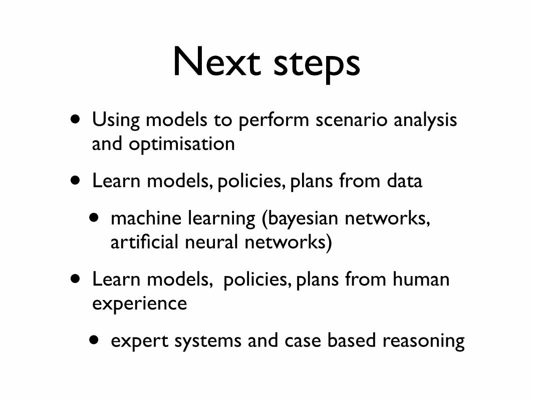
Next steps• Using models to perform scenario analysis

and optimisation

• Learn models, policies, plans from data

• machine learning (bayesian networks, artificial neural networks)

• Learn models, policies, plans from human experience

• expert systems and case based reasoning