modelling, forecasting and testing decisions for seasonal

Acta Polytechnica Hungarica Vol. 17, No. 10, 2020

– 149 –

Modelling, Forecasting and Testing Decisions

for Seasonal Time Series in Tourism

Cvetko Andreeski1, Daniela Mechkaroska

2

Faculty of Tourism and Hospitality – Ohrid, University „St. Kliment Ohridski“ –

Bitola, 7000 Bitola1

Faculty of Computer Science and Engineering, Skopje, Ss. Cyril and Methodius

University, 1000 Skopje, Macedonia2

[email protected], [email protected]

2

Abstract: Time series analysis for basic tourism parameters, in the countries of the Balkan

Peninsula, have been emphasized in recent research. Moreover, some of them have also

shown a trend, aside from the rising variance during the period-heteroscedasticity. All of

these characteristics of a time series of tourist demand, result in them being a great

challenge for modeling. Therefore, there are different types of models that can be

implemented for the modeling of a time series, which include accentuated seasonal

components. Throughout this paper, multiple tests are performed using several parameters

of the time series, with the ARIMA model, in an attempt to find any influence on the fit and

validity of the model. For the accepted models, series are predicted for a year in advance

and, in addition, a method of testing the decisions made by authorities in the field of

tourism is presented.

Keywords: time series; modelling; parameters; forecasting; testing; decisions

1 Introduction

The modeling and forecasting of a time series plays a vital role in the process of

planning and decision making in the tourism industry, which accounts for the vast

number of papers on these issues. In the paper [15], modeling and forecasting is

made for basic tourism parameters, from 1953-2014, sampled as annual data. This

series is a challenge for modeling, as it contains two structural breaks. For the

modeling, a standard ARIMA model is implemented according to what can be

found in [2]. Alternatively, in paper [20], the authors used several competing

models, mainly based on models for time series analysis and commenting on the

results of modeling and forecasting of a series of arrivals in Australia. On the other

hand, in paper [1] and [6] the main aim of research is the comparison between

linear ARIMA models and non-linear models based on artificial neural networks.

In paper [1] we can find an exploration of their performances for modeling time

C. Andreeski et al. Modelling, Forecasting and Testing Decisions for Seasonal Time Series in Tourism

– 150 –

series with existing break(s). Nevertheless, many authors have worked on time

series modeling with seasonal components by using neural networks [3] [6] [13]

[19], as time series with a significant seasonal component are important in different

areas of research like economy [7], climate forecast [17], biology [18], medicine

[8], etc. Aside from their performances in modeling, especially in modeling time

series with occurring structural break(s), these models are much more complex than

linear models. They have the potential problem of getting values of weights from

the local minimum, so the results of forecasting can be disappointing, or fail to

meet previous expectations based on the results of modeling [6] [3]. In this paper,

we have analyzed time series of arrived domestic and foreign tourists with monthly

data from two landlocked countries on the Balkan Peninsula: The Republic of

Macedonia and the Republic of Serbia for a period of nine years. Whilst all the

analyzed series have accentuated seasonal behavior, an upward trend is present, as

well. All those characteristics of the series present a significant challenge for

successful modeling and forecasting. ARIMA models will be used in the process of

modeling and accordingly, different parameters of them will be tested to choose the

best one. Correspondingly, the final chosen model will be tested for validity and

forecast performance. Additionally, a forecast of future values of arrived tourists

for the current year has been created. This paper presents a way of testing the

decisions made in both countries aimed at supporting the growth of tourism. A few

of them will be tested in different intervals for the impact that they have on the

progress of tourism via increment on number of arrived tourists.

2 Analysis of Time Series

For the modeling, two different time series are used for each country: one

concerns the domestic tourists visiting the Republic of Macedonia for the period

from 01:2010 until 08:2017, and the other a series of arrived foreign tourists

during the same interval. Despite the similarities of the two, we can detect

different characteristics and behavior of the series. Both series have been

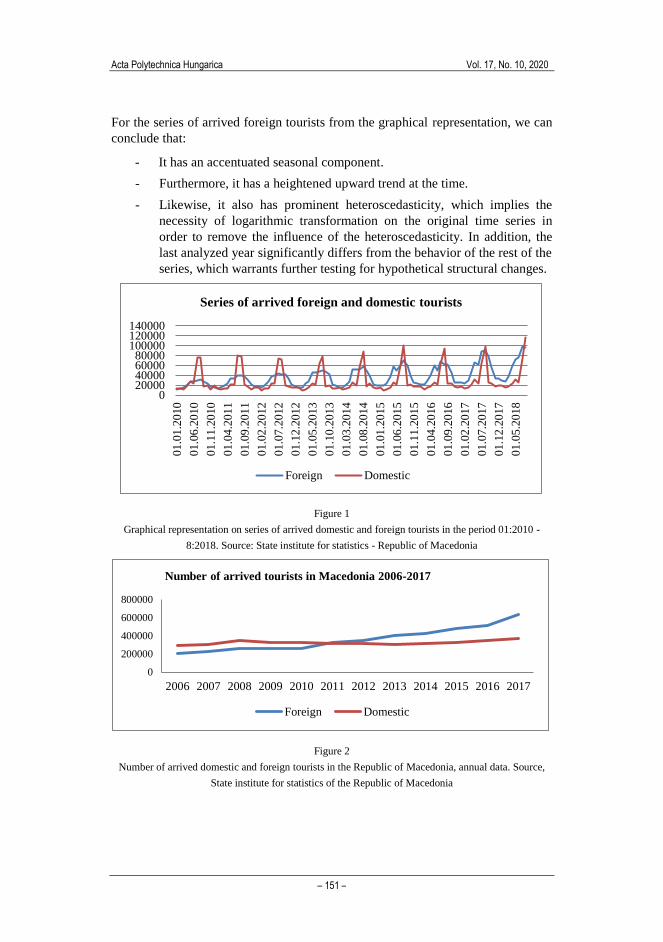
presented for the analyzed time increment, in the Republic of Macedonia in Figure

1. From the graphical representation of the time series, several features may be

noticed.

For the series of arrived domestic tourists we can conclude the following:

- The series has an accentuated seasonal component, much more heightened

than is the case for the series of arrived foreign tourists at the same time.

- This series does not have a trend, although there is variation around an

average value. It can be visible if we present data on an annual level.

- It has weak heteroscedasticity that should be tested.


– 151 –

For the series of arrived foreign tourists from the graphical representation, we can

conclude that:

- It has an accentuated seasonal component.

- Furthermore, it has a heightened upward trend at the time.

- Likewise, it also has prominent heteroscedasticity, which implies the

necessity of logarithmic transformation on the original time series in

order to remove the influence of the heteroscedasticity. In addition, the

last analyzed year significantly differs from the behavior of the rest of the

series, which warrants further testing for hypothetical structural changes.

Figure 1

Graphical representation on series of arrived domestic and foreign tourists in the period 01:2010 -

8:2018. Source: State institute for statistics - Republic of Macedonia

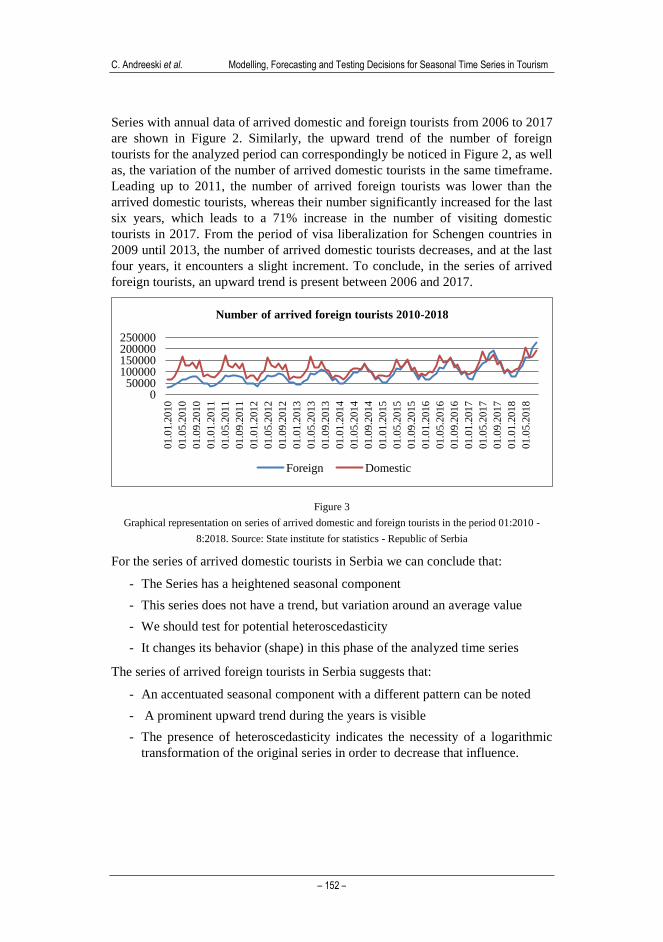
Figure 2

Number of arrived domestic and foreign tourists in the Republic of Macedonia, annual data. Source,

State institute for statistics of the Republic of Macedonia

020000400006000080000

100000120000140000

01.0

1.2

010

01.0

6.2

010

01.1

1.2

010

01.0

4.2

011

01.0

9.2

011

01.0

2.2

012

01.0

7.2

012

01.1

2.2

012

01.0

5.2

013

01.1

0.2

013

01.0

3.2

014

01.0

8.2

014

01.0

1.2

015

01.0

6.2

015

01.1

1.2

015

01.0

4.2

016

01.0

9.2

016

01.0

2.2

017

01.0

7.2

017

01.1

2.2

017

01.0

5.2

018

Series of arrived foreign and domestic tourists

Foreign Domestic

0

200000

400000

600000

800000

2006 2007 2008 2009 2010 2011 2012 2013 2014 2015 2016 2017

Number of arrived tourists in Macedonia 2006-2017

Foreign Domestic


– 152 –

Series with annual data of arrived domestic and foreign tourists from 2006 to 2017

are shown in Figure 2. Similarly, the upward trend of the number of foreign

tourists for the analyzed period can correspondingly be noticed in Figure 2, as well

as, the variation of the number of arrived domestic tourists in the same timeframe.

Leading up to 2011, the number of arrived foreign tourists was lower than the

arrived domestic tourists, whereas their number significantly increased for the last

six years, which leads to a 71% increase in the number of visiting domestic

tourists in 2017. From the period of visa liberalization for Schengen countries in

2009 until 2013, the number of arrived domestic tourists decreases, and at the last

four years, it encounters a slight increment. To conclude, in the series of arrived

foreign tourists, an upward trend is present between 2006 and 2017.

Figure 3

Graphical representation on series of arrived domestic and foreign tourists in the period 01:2010 -

8:2018. Source: State institute for statistics - Republic of Serbia

For the series of arrived domestic tourists in Serbia we can conclude that:

- The Series has a heightened seasonal component

- This series does not have a trend, but variation around an average value

- We should test for potential heteroscedasticity

- It changes its behavior (shape) in this phase of the analyzed time series

The series of arrived foreign tourists in Serbia suggests that:

- An accentuated seasonal component with a different pattern can be noted

- A prominent upward trend during the years is visible

- The presence of heteroscedasticity indicates the necessity of a logarithmic

transformation of the original series in order to decrease that influence.

050000

100000150000200000250000

01

.01.2

01

0

01

.05.2

01

0

01

.09.2

01

0

01

.01.2

01

1

01

.05.2

01

1

01

.09.2

01

1

01

.01.2

01

2

01

.05.2

01

2

01

.09.2

01

2

01

.01.2

01

3

01

.05.2

01

3

01

.09.2

01

3

01

.01.2

01

4

01

.05.2

01

4

01

.09.2

01

4

01

.01.2

01

5

01

.05.2

01

5

01

.09.2

01

5

01

.01.2

01

6

01

.05.2

01

6

01

.09.2

01

6

01

.01.2

01

7

01

.05.2

01

7

01

.09.2

01

7

01

.01.2

01

8

01

.05.2

01

8

Number of arrived foreign tourists 2010-2018

Foreign Domestic


– 153 –

Each series should be tested for possible structural breaks1.

Figure 4 portrays the series with annual data of arrived domestic and foreign

tourists between 2010 and 2017 – Republic of Serbia, from which the upward

trend of the number of foreign tourists can be observed.

On the other hand, the number of arrived domestic tourists does not show a

specific trend, as it has variations around the average number of arrived tourists.

Beside the fact that the series of arrived foreign tourists has a constant upward

trend, the number of domestic tourists is greater than the number of arrived

foreign tourists.

Figure 4

Number of arrived domestic and foreign tourists in the Republic of Serbia, annual data. Source, State

institute for statistics of the Republic of Serbia

3 Modeling of Time Series

Autoregressive moving average model (ARMA) for stationary time series is a

linear structure of two polynomials, one for the auto-regression (AR) and the

second for the moving average (MA).

A stationary ARMA(p,q) model is defined as a linear sequence of autoregressive

random variables Xt, and moving average random variables Yt with zero mean

value and constant variance provided by (1):

Xt-φtXt-1-…-φpXt-p=Yt+θ1Yt-1+…+θqYt-q (1)

If the time series is non-stationary, we need to differentiate the series in order to

get a stationary one. In this case we have an ARIMA(p,d,q) process where d is a

1 Structural break is an abruptly change of time series at a point in time. This variation

could involve a change in mean or a change in the other parameters of the process that

produce(s) the series.

0

500000

1000000

1500000

2000000

2010 2011 2012 2013 2014 2015 2016 2017

Number of arrived tourists in the Republic of Serbia 2010-2017

Domestic Foreign


– 154 –

non-negative integer such that (1-B)dXt is a causal ARMA(p,q) process [5]. All the

analyzed time series in this paper are sampled by monthly data.

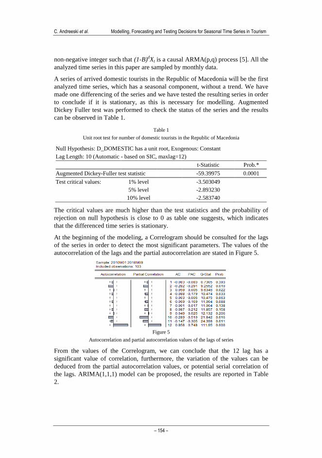
A series of arrived domestic tourists in the Republic of Macedonia will be the first

analyzed time series, which has a seasonal component, without a trend. We have

made one differencing of the series and we have tested the resulting series in order

to conclude if it is stationary, as this is necessary for modelling. Augmented

Dickey Fuller test was performed to check the status of the series and the results

can be observed in Table 1.

Table 1

Unit root test for number of domestic tourists in the Republic of Macedonia

Null Hypothesis: D_DOMESTIC has a unit root, Exogenous: Constant

Lag Length: 10 (Automatic - based on SIC, maxlag=12)

t-Statistic Prob.*

Augmented Dickey-Fuller test statistic -59.39975 0.0001

Test critical values: 1% level -3.503049

5% level -2.893230

10% level -2.583740

The critical values are much higher than the test statistics and the probability of

rejection on null hypothesis is close to 0 as table one suggests, which indicates

that the differenced time series is stationary.

At the beginning of the modeling, a Correlogram should be consulted for the lags

of the series in order to detect the most significant parameters. The values of the

autocorrelation of the lags and the partial autocorrelation are stated in Figure 5.

Figure 5

Autocorrelation and partial autocorrelation values of the lags of series

From the values of the Correlogram, we can conclude that the 12 lag has a

significant value of correlation, furthermore, the variation of the values can be

deduced from the partial autocorrelation values, or potential serial correlation of

the lags. ARIMA(1,1,1) model can be proposed, the results are reported in Table

2.


– 155 –

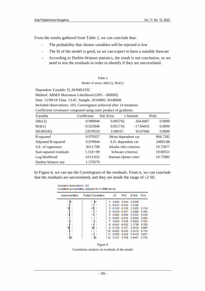
From the results gathered from Table 2, we can conclude that:

- The probability that chosen variables will be rejected is low

- The fit of the model is good, so we can expect to have a suitable forecast

- According to Durbin-Watson statistics, the result is not conclusive, so we

need to test the residuals in order to identify if they are uncorrelated.

Table 2

Model of series AR(12), MA(1)

Dependent Variable: D_DOMESTIC

Method: ARMA Maximum Likelihood (OPG - BHHH)

Date: 12/09/18 Time: 13:47, Sample: 2010M02 2018M08

Included observations: 103, Convergence achieved after 14 iterations

Coefficient covariance computed using outer product of gradients

Variable Coefficient Std. Error t-Statistic Prob.

AR(12) 0.990949 0.003742 264.8407 0.0000

MA(1) -0.922846 0.051716 -17.84435 0.0000

SIGMASQ 12678529 1188167. 10.67066 0.0000

R-squared 0.979357 Mean dependent var 994.7282

Adjusted R-squared 0.978944 S.D. dependent var 24903.88

S.E. of regression 3613.708 Akaike info criterion 19.72877

Sum squared residuals 1.31E+09 Schwarz criterion 19.80551

Log likelihood -1013.032 Hannan-Quinn criter. 19.75985

Durbin-Watson stat 1.579279

In Figure 6, we can see the Correlogram of the residuals. From it, we can conclude

that the residuals are uncorrelated, and they are inside the range of ±2 SE.

Figure 6

Correlation analysis on residuals of the model


– 156 –

The results provided in Table 3 imply that there is no heteroscedasticity of the

residuals, and the model is valid. Hence, the residuals are uncorrelated and there is

no heteroscedasticity in this series. This model grants us an opportunity to forecast

future values of the series, aside from covering almost 98% of the variance of

differenced series.

Table 3

Heteroscedasticity White Test on residuals

Heteroskedasticity Test: White

F-statistic 172.8046 Prob. F(6,96) 0.0000

Obs*R-squared 94.27140 Prob. Chi-Square(6) 0.0000

Scaled explained SS 305.8439 Prob. Chi-Square(6) 0.0000

Figure 7 portrays an in sample forecast of the values 01-08.2018.

-10,000

0

10,000

20,000

30,000

40,000

50,000

M1 M2 M3 M4 M5 M6 M7 M8

2018

D_DOMASNI D_DOMASNIF

--- D_DOMESTIC

---D_DOMESTICF

Figure 7

In sample forecasting of the series for 2018

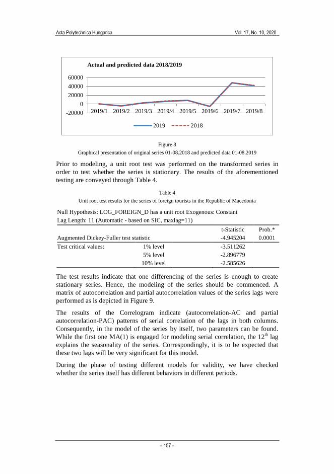
Figure 8 represents the forecast of values for the analyzed series of arrived

domestic tourists in 2019, and illustrates a comparison of the values with the

previous year.

From there, we can deduct that the series of arrived domestic tourists in 2018 and

the predicted values for 2019 are almost identical. The difference within the entire

predicted timeframe is minor, but taking into consideration the fact that a trend

was not present in the series, this result is to be expected.

The second modeled series, is the series of arrived foreign tourists in the Republic

of Macedonia in the period between 01.2010 and 08.2018. This series is more

complex for identification, taking into consideration the fact that this series has a

trend, seasonal component, and evident heteroscedasticity. As can be seen by

these characteristics of the series, a logarithmic transformation on the original

series has been conducted, as well as differencing the series in order to create a

stationary one.


– 157 –

Figure 8

Graphical presentation of original series 01-08.2018 and predicted data 01-08.2019

Prior to modeling, a unit root test was performed on the transformed series in

order to test whether the series is stationary. The results of the aforementioned

testing are conveyed through Table 4.

Table 4

Unit root test results for the series of foreign tourists in the Republic of Macedonia

Null Hypothesis: LOG_FOREIGN_D has a unit root Exogenous: Constant


t-Statistic Prob.*



5% level -2.896779

10% level -2.585626

The test results indicate that one differencing of the series is enough to create

stationary series. Hence, the modeling of the series should be commenced. A

matrix of autocorrelation and partial autocorrelation values of the series lags were

performed as is depicted in Figure 9.

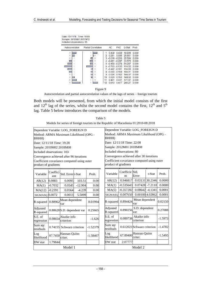
The results of the Correlogram indicate (autocorrelation-AC and partial

autocorrelation-PAC) patterns of serial correlation of the lags in both columns.

Consequently, in the model of the series by itself, two parameters can be found.

While the first one MA(1) is engaged for modeling serial correlation, the 12th

lag

explains the seasonality of the series. Correspondingly, it is to be expected that

these two lags will be very significant for this model.

During the phase of testing different models for validity, we have checked

whether the series itself has different behaviors in different periods.

-20000

0

20000

40000

60000

2019/1 2019/2 2019/3 2019/4 2019/5 2019/6 2019/7 2019/8

Actual and predicted data 2018/2019

2019 2018


– 158 –

Figure 9

Autocorrelation and partial autocorrelation values of the lags of series – foreign tourists

Both models will be presented, from which the initial model consists of the first

and 12th

lag of the series, whilst the second model contains the first, 12th

and 5th

lag. Table 5 below introduces the comparison of the models.

Table 5

Models for series of foreign tourists in the Republic of Macedonia 01:2010-08:2018

Dependent Variable: LOG_FOREIGN D

Method: ARMA Maximum Likelihood (OPG -

BHHH)

Date: 12/11/18 Time: 19:28

Sample: 2010M02 2018M08

Included observations: 103

Convergence achieved after 96 iterations

Coefficient covariance computed using outer

product of gradients

Variable Coeffici

ent Std. Error t-Stat Prob.

AR(12) 0.9883 0.0095 103.51 0.00

MA(1) -0.7032 0.0545 -12.904 0.00

MA(12) -0.2391 0.0564 -4.239 0.00

SIGMASQ 0.0072 0.0013 5.5099 0.00

R-squared 0.88962 Mean dependent

var 0.01994

Adjusted

R-squared 0.88628 S.D. dependent var 0.25665

S.E. of

regression 0.08654

Akaike info

criterion -1.626

Sum sqr

residuals 0.74155 Schwarz criterion -1.52379

Log

likelihood 87.7450

Hannan-Quinn

criter. -1.58467

DW stat 1.79844

Dependent Variable: LOG_FOREIGN D

Method: ARMA Maximum Likelihood (OPG -

BHHH)

Date: 12/11/18 Time: 22:08

Sample: 2012M01 2018M08





Variable Coefficie

nt

Std.

Error t-Stat Prob.

AR(12) 0.946817 0.03131 30.2346 0.0000

MA(1) -0.535643 0.07428 -7.2110 0.0000

MA(5) -0.357282 0.08642 -4.1341 0.0001

SIGMASQ 0.007650 0.00189 4.02862 0.0001

R-squared 0.894424 Mean dependent

var 0.02150

Adjusted

R-squared 0.890256

S.D. dependent

var 0.27088

S.E. of

regression 0.089738

Akaike info

criterion -1.5973

Sum sqr


Log

likelihood 67.89400

Hannan-Quinn

criter. -1.5495

DW stat 2.07777

Model 1 Model 2


– 159 –

Several conclusions can be deducted from the results of the preparation of model

1:

- Incorporated independent variables have low probability of rejection

from the model, or high value of t-statistics

- The displayed model covers more than 88% of the variance of the series

- Durbin-Watson - DW statistics has a value close to 2 which can be an

indicator for absence of serial correlation of residuals. However, further

testing is necessary for assessing the hypothetical correlation of the

residuals.

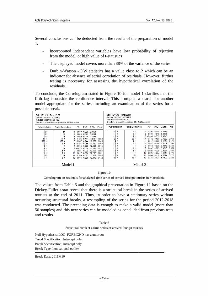
To conclude, the Correlogram stated in Figure 10 for model 1 clarifies that the

fifth lag is outside the confidence interval. This prompted a search for another

model appropriate for the series, including an examination of the series for a

possible break.

Model 1 Model 2

Figure 10

Correlogram on residuals for analyzed time series of arrived foreign tourists in Macedonia

The values from Table 6 and the graphical presentation in Figure 11 based on the

Dickey-Fuller t-stat reveal that there is a structural break in the series of arrived

tourists at the end of 2011. Thus, in order to have a stationary series without

occurring structural breaks, a resampling of the series for the period 2012-2018

was conducted. The preceding data is enough to make a valid model (more than

50 samples) and this new series can be modeled as concluded from previous tests

and results.

Table 6

Structural break at a time series of arrived foreign tourists

Null Hypothesis: LOG_FOREIGND has a unit root

Trend Specification: Intercept only

Break Specification: Intercept only

Break Type: Innovational outlier

Break Date: 2011M10


– 160 –

Break Selection: Minimize Dickey-Fuller t-statistic

Lag Length: 11 (Automatic - based on Schwarz information criterion, maxlag=12)

t-Statistic Prob.*

Augmented Dickey-Fuller test statistic -5.781147 < 0.01

Test critical

values:

1% level -4.949133

5% level -4.443649

10%level -4.193627

Results on modeling for this series can be subtracted from Table 5, model 2. This

model has the following characteristics:

- Incorporated independent variables have low probability of rejection from

the model, or high value of t-statistics

- The represented model covers more than 89% of the variance of the series

- The Durbin-Watson statistics has a value close to 2 which can be an

indicator for the absence of serial correlation of residuals, however, further

testing of the residuals is required

A comparison of Akaike and Hannan Quinn information criterion indicates that

model 2 has lower values for both criteria, which consequently suggests that this

model is more applicable than model 1. As models have the same number of

independent variables, this does not affect the results of criteria. Furthermore, the

results of the Correlogram on the residuals of model 2 imply that residuals are

uncorrelated, and subsequently, there are no values outside the confidence

interval, thus model 2 is a valid model for this series.

-5.8

-5.6

-5.4

-5.2

-5.0

-4.8

-4.6

2011 2012 2013 2014 2015 2016 2017 2018

Dickey-Fuller t-statistics

Figure 11

Structural break graph at the end of 2011 – series of foreign tourists


– 161 –

Figure 12

Original and predicted time series – arrived foreign tourists, Republic of Macedonia

Implementing the model that has proven to be superior, we can make a forecast

for 2019. The results acquired from the use of the aforementioned model are

portrayed in Figure 12. In addition, from the two graphs showcased in Figure 12,

the first one is an in-sample forecast on-log and differenced series, while the

second one is the forecast for 2019 vs 2018.

The following analysis and modeling on the series of arrived tourists in the

Republic of Macedonia is about the first series of domestic tourists.

Before undertaking the analysis, the series should be tested for conceivable break

point(s). The graphical presentation of the series in Figure 3 shows different

behaviors of the series during the analyzed period. The completed unit root break

test is documented in Figure 13.

Null Hypothesis: D_DOMESTIC has a

unit root

-28

-24

-20

-16

-12

-8

-4

0

2011 2012 2013 2014 2015 2016 2017 2018





Break Date: 2015M05

Break Selection: Minimize Dickey-Fuller

t-statistic

Lag Length: 10 (Automatic - based on

Schwarz information criterion,

maxlag=12)

t-Stat Prob.*

ADF test -25.4579 < 0.01

Test critical

values:

1% level -4.9491

5% level -4.4436

10%level -4.1936

Figure 13

Unit root break test on the time series of arrived domestic tourists

0

20000

40000

60000

80000

100000

120000

1 2 3 4 5 6 7 8

Forecast for 2019 and data for 2018

2018 2019


– 162 –

The results in Figure 13, suggest that there is a break point in the series detected in

2015. Resampling the series 01:2015-08:2015 reveals that the number of data in

the new series is slightly higher than the minimum series of 30 samples. The

resampling and differencing of the series in order to get a stationary one was

performed, from which results can be noted from Table 7.

Table 7

Unit root test results for the series of domestic tourists in the Republic of Serbia

Null Hypothesis: D_DOMESTIC has a unit root, Exogenous: Constant


t-Statistic Prob.*



5% level -2.929734

10% level -2.603064

As can be seen by the results from Table 7, the differenced time series is a

stationary one. This concludes that the probability of rejection of null hypothesis

is quite low. At this point, a Correlogram can be created in order to detect the

crucial lags in the series. It has an evident trend and heteroscedasticity, which has

prompted both a logarithmic transformation, and first lag differencing on the

series. The Correlogram for the transformed and differenced series is presented in

Figure 14.

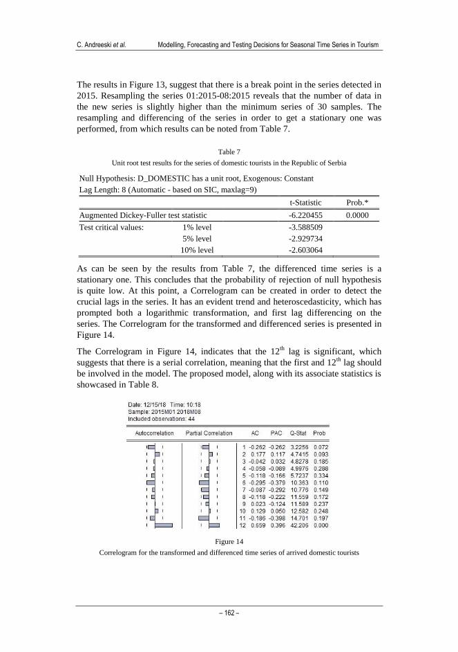
The Correlogram in Figure 14, indicates that the 12th

lag is significant, which

suggests that there is a serial correlation, meaning that the first and 12th

lag should

be involved in the model. The proposed model, along with its associate statistics is

showcased in Table 8.

Figure 14

Correlogram for the transformed and differenced time series of arrived domestic tourists


– 163 –

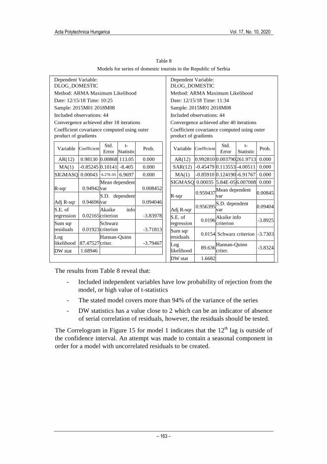
Table 8

Models for series of domestic tourists in the Republic of Serbia

Dependent Variable:

DLOG_DOMESTIC

Method: ARMA Maximum Likelihood

Date: 12/15/18 Time: 10:25

Sample: 2015M01 2018M08





Variable Coefficient

Std.

Error

t-

Statistic Prob.

AR(12) 0.98130 0.00868 113.05 0.000

MA(1) -0.85245 0.10141 -8.405 0.000

SIGMASQ 0.00043 6.27E-05 6.9697 0.000

R-sqr 0.94942

Mean dependent

var 0.008452

Adj R-sqr 0.94696

S.D. dependent

var 0.094046

S.E. of

regression 0.02165

Akaike info

criterion -3.83978

Sum sqr

residuals 0.01923

Schwarz

criterion -3.71813

Log

likelihood 87.47527

Hannan-Quinn

criter. -3.79467

DW stat 1.68946

Dependent Variable:

DLOG_DOMESTIC

Method: ARMA Maximum Likelihood

Date: 12/15/18 Time: 11:34

Sample: 2015M01 2018M08





Variable Coefficient

Std.

Error

t-

Statistic Prob.

AR(12) 0.992810 0.003790 261.9713 0.000

SAR(12) -0.45479 0.113553 -4.00511 0.000

MA(1) -0.85910 0.124190 -6.91767 0.000

SIGMASQ 0.00035 5.84E-05 6.007008 0.000

R-sqr 0.959437

Mean dependent

var 0.00845

Adj R-sqr 0.956395

S.D. dependent

var 0.09404

S.E. of

regression 0.0196

Akaike info

criterion -3.8925

Sum sqr


Log

likelihood 89.636

Hannan-Quinn

criter. -3.8324

DW stat 1.6682

The results from Table 8 reveal that:

- Included independent variables have low probability of rejection from the

model, or high value of t-statistics

- The stated model covers more than 94% of the variance of the series

- DW statistics has a value close to 2 which can be an indicator of absence

of serial correlation of residuals, however, the residuals should be tested.

The Correlogram in Figure 15 for model 1 indicates that the 12th

lag is outside of

the confidence interval. An attempt was made to contain a seasonal component in

order for a model with uncorrelated residuals to be created.


– 164 –

Figure 15

Correlation of residuals for both models: series of arrived domestic tourists – Serbia

The residuals of the second model are not correlated, which indicates that it is to

be rendered as valid for representing this time series. Suitably, the results of

modeling given in Table 8 specify that Akaike and Hannan Quinn criteria have

lower values for the first model, due to the number of independent variables. Then

again, model 1 cannot be selected, as it is not relevant for this time series. What

follows is a forecast calculated by the model. Figure 16 is presenting an in sample

forecast.

Figure 16

In sample and out of sample forecast for time series of arrived domestic tourists – Serbia

The last time series analyzed in this paper is the series of arrived foreign tourists

in the Republic of Serbia, as can be deducted from Figure 3. As concluded earlier,

this series should be tested for impending structural breaks, as there are evident

differences in the behavior of the series over a longer period. This time series has

an accentuated trend and heteroscedasticity. As means to eliminate the

heteroscedasticity and trend a transformation on the series was performed, which

contained a differentiation and log transformation. Likewise, whether the time

series is stationary was tested with a unit root test.

0

200000

400000

1 2 3 4 5 6 7 8

Original series for 2018 and predicted values

2018 2019


– 165 –

The results specified in Table 9 indicate that the value of t-statistics is lower than

the critical values, and the probability to reject null hypothesis of stationary series

is very low. Henceforth, the resulting time series is stationary.

Table 9

Results of unit root test for the series of arrived foreign tourists – Republic of Serbia

Null Hypothesis: LOGD_FOREIGN has a unit root, Exogenous: Constant


t-Statistic Prob.*



5% level -2.904198

10% level -2.589562

As depicted in Figure 17, a test was performed to examine the series for potential

structural breaks.

Null Hypothesis: LOGD_FOREIGN has a unit root




Break Date: 2017M02

Break Selection: Minimize DF t-statistic

Lag Length: 10 (Automatic - based on Schwarz information criterion, maxlag=10)

t-Statistic Prob.*

ADF test -15.823 < 0.01

Test

critical

values:

1% level -4.9491

5% level -4.4436

10% level -4.1936

-17.0

-16.5

-16.0

-15.5

-15.0

-14.5

-14.0

-13.5

I II III IV I II III IV I II III IV I II III IV I II III IV I II III

2013 2014 2015 2016 2017 2018


Figure 17

Structural break unit root test. Time series of foreign tourists in the Republic of Serbia

Additionally, the results represented in Figure 17 show that this series has a

structural break at the beginning of 2017, meaning that, there is not enough

sample data to serve as basis for a valid model. Models for identification of time

series with existing structural breaks can be found in literature, such as models

based on Artificial Neural Networks, yet their structure is very complex. In these

models, the number of variables is much higher than the variables from ARIMA,

and the forecasting is not as accurate as those created with linear models [3] [4].

Some authors [6] propose a combination of linear and non-linear models to get the

best results, even though these models are more complex, and in most cases are

hardly superior to linear models. They test in [9] [6] [19], the models going by the

values of the residuals and the error between the original series and model with

calculated MAPE and MAE errors.


– 166 –

In this paper, the accuracy of the models is between 88% and 97%, although that

is not the main issue, but only one aspect of designing a valid model. The reasons

for changes of the behavior of the series, as well as the period of the changes need

to be identified. That is why the design of the model for this series will not be

continued.

4 Analysis of Government Decisions Concerning

Tourism

For the analyzed countries in the Balkans, the government decisions for the

improvement of tourism have been considered as well. Both of these countries

have subsidies for tourism. Granted, both countries have different approaches

toward the type of subsidies, the choices for each of them were tested.

Subsequently, the analysis of the implemented strategies in the Republic of

Macedonia was conducted first, in which the period 2011-2018 was considered in

order to make an appropriate analysis.

The unit root test for structural break(s) was selected as a valid methodology on

testing decisions, where structural break(s) in time series is an abrupt change at a

point in time. This change could involve a change in mean or the other parameters

of the process that produce time series, such as variance or trend.

The most important assumption under the unit root [11] is that the random shocks

have permanent effects on the long-run level of series. Correspondingly, these

findings were challenged by [14], who argues that in the presence of a structural

break, the standard ADF tests are biased towards the non-rejection of the null

hypothesis [10]. Evidence of such an example can be found in the analyzed series

of arrived foreign tourists in the Republic of Serbia, within this paper. According

to the ADF test, the series is stationary after the first difference, but that shock is

not on the long-run level of the series as can be concluded after the unit root break

test.

Contrarily, Perron proposes a modified Dickey Fuller - (DF) unit root test with

included dummy variables, to test the known or exogenous structural break. There

are three types of possible structural breaks: First, changes in level of the series,

second, changing of the trend (slope) in the series and third, a combination of the

first and second break. Those three types are summed in the following equations:

𝑥𝑡 = 𝛼0 + 𝛼1𝐷𝑈𝑡 + 𝑑(𝐷𝑇𝐵)𝑡 + 𝛽𝑡 + 𝜌𝑥𝑡−1 + ∑ 𝜙𝑖Δ𝑥𝑡−1 + 𝜀𝑡𝑝𝑖=1 (2)

𝑥𝑡 = 𝛼0 + 𝛾𝐷𝑇𝑡 + 𝛽𝑡 + 𝜌𝑥𝑡−1 + ∑ 𝜙𝑖Δ𝑥𝑡−1 + 𝜀𝑡𝑝𝑖=1 (3)

𝑥𝑡 = 𝛼0 + 𝛼1𝐷𝑈𝑡 + 𝑑(𝐷𝑇𝐵)𝑡 + 𝛾𝐷𝑇𝑡 + 𝛽𝑡 + 𝜌𝑥𝑡−1 + ∑ 𝜙𝑖Δ𝑥𝑡−1 + 𝜀𝑡 𝑝𝑖=1 (4)


– 167 –

Where 𝐷𝑈𝑡 is the intercept dummy which tests the change in the level; 𝐷𝑇𝑡 is the

slope dummy which tests the slope in some interval of the series and TB is a date

of a structural break. All models have a unit root with a break under the null

hypothesis [10].

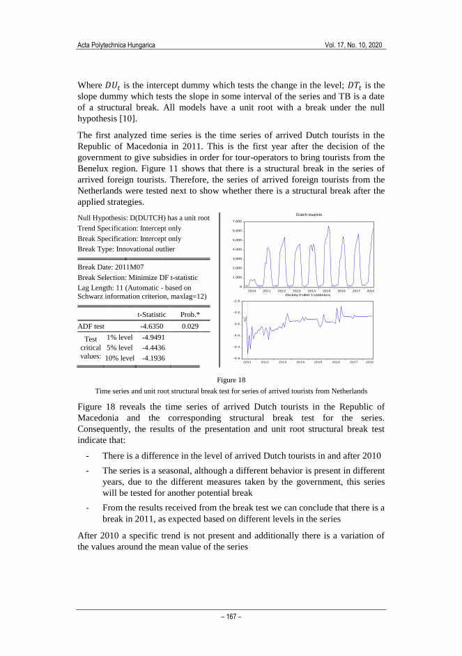
The first analyzed time series is the time series of arrived Dutch tourists in the

Republic of Macedonia in 2011. This is the first year after the decision of the

government to give subsidies in order for tour-operators to bring tourists from the

Benelux region. Figure 11 shows that there is a structural break in the series of

arrived foreign tourists. Therefore, the series of arrived foreign tourists from the

Netherlands were tested next to show whether there is a structural break after the

applied strategies.

Null Hypothesis: D(DUTCH) has a unit root




Break Date: 2011M07



Schwarz information criterion, maxlag=12)

t-Statistic Prob.*

ADF test -4.6350 0.029

Test

critical values:

1% level -4.9491

5% level -4.4436

10% level -4.1936

0

1,000

2,000

3,000

4,000

5,000

6,000

7,000

2010 2011 2012 2013 2014 2015 2016 2017 2018

Dutch tourists

-4.8

-4.4

-4.0

-3.6

-3.2

-2.8

2011 2012 2013 2014 2015 2016 2017 2018


Figure 18

Time series and unit root structural break test for series of arrived tourists from Netherlands

Figure 18 reveals the time series of arrived Dutch tourists in the Republic of

Macedonia and the corresponding structural break test for the series.

Consequently, the results of the presentation and unit root structural break test

indicate that:

- There is a difference in the level of arrived Dutch tourists in and after 2010

- The series is a seasonal, although a different behavior is present in different

years, due to the different measures taken by the government, this series

will be tested for another potential break

- From the results received from the break test we can conclude that there is a

break in 2011, as expected based on different levels in the series

After 2010 a specific trend is not present and additionally there is a variation of

the values around the mean value of the series


– 168 –

Another time series of arrived tourists from Scandinavian countries will be tested

as well. A time series of arrived tourists from Sweden was taken as an example. In

the Official Gazette of the Republic of Macedonia, No 53 published on 11 of April

2013, the government of the Republic of Macedonia has announced subsidies for

tourists from Sweden amounting to 25 euros per tourist. Figure 19 presents the

time series of arrived tourists from Sweden, including a unit root break test for this

series. The graph of the series indicates that:

- This time series has a trend and an accentuated heteroscedasticity.What is

more, the increase in the number of foreign tourists arrived in 2017

compared to 2010 is 363%

- Different behavior of the series in different years is evidenced, however, a

proper test should be conducted such as a unit root test for a structural

break

- There is no significant change in the level of the series in 2013, or 2014 as

noted in the series of arrived tourists from the Netherlands.

The results given in the table of the unit root break test reveal that there is a

structural break in the series in 2017. Contrarily, this structural break cannot be

connected with the decision of the government in 2013. This leads to a conclusion

that this decision did not bring the expected results measured by the increment in

the number of arrived tourists from Sweden in the Republic of Macedonia.

Moreover, the positive trend in the series can also be a result of the number of

established direct air lines from Sweden to the Republic of Macedonia.2 An added

difference between the decision made for tourists from Benelux and one for

tourists from Scandinavian countries is that subsidies for Scandinavian tourists is

25 euros per tourist, despite the amount of 65 euros for the arrived tourists from

Benelux.

Nonetheless, subsidies in the Republic of Serbia have a different character and

purpose in relation to subsidies in the Republic of Macedonia.

In Serbia, judging by the annual competitions for tourism subsidies envisaged

under the established Strategy for development of tourism in the Republic of

Serbia for the time between 2016 and 20253, subsidies may be received by

domestic legal entities for the following purposes: promotion of tourism products,

progress of satellite account statistics, education and training in tourism,

arrangement of space, creation of planning documentation, arrangement of public

areas, etc.

2 In 2013 airline company Wizzair established direct lines from Skopje to Stockholm

and Goteborg 3 http://mtt.gov.rs/download/3/strategija.pdf


– 169 –

Null Hypothesis: D(SWEDISH) has a unit root




Break Date: 2017M05



Schwarz information criterion, maxlag=12)

t-Statistic Prob.*

ADF test statistic -6.7050 < 0.01

Test

critical

values:

1% level -4.9491

5% level -4.4436

10% level -4.1936

0

400

800

1,200

1,600

2,000

2010 2011 2012 2013 2014 2015 2016 2017 2018

Tourists from Sweden

-7.0

-6.5

-6.0

-5.5

-5.0

-4.5

-4.0

-3.5

-3.0

2011 2012 2013 2014 2015 2016 2017 2018


Figure 19

Time series and unit root structural break test for time series of arrived tourists from Sweden

This diverts the attention to the previous analysis of the series of arrived tourists in

the Republic of Serbia. Subsequently, for foreign tourists, the structural break is at

the beginning of 2017, which may indicate a result of the measures provided for

the Tourism Development Strategy 2016-2025.

Conclusions

From our conducted analysis on time series of the number of visiting tourists in

two neighboring countries in the Balkans, we can conclude, that in spite of the

similarities in the characteristics of the series, the generated models can differ.

Even though all of them have seasonal components and a significant serial

correlation, each model has unique characteristics. What is more, all models are

tested for validity, adding to the attempt at creating a concurrent model, which is

chosen as per the results of the accompanied information criteria. Moreover, one

of the essential parts in the analysis is the presence of any structural break(s) in the

time series, which can influence choices, or events that have happened during a

given period of the analysis. Likewise, they can serve as a basis for testing

decisions of the Government or other Governmental body, that are responsible for

any strategies and assessments designed to improve Tourism in their country. As

deduced from the analysis, some implemented strategies have an impact on the

advancement of Tourism, whereas some of them do not. However, the main goals

in the development of Tourism, is the growth of the number of arriving foreign

tourists and to ensure that the target has been reached for the concerned country.

References

[1] Andreeski, Cvetko, and Pandian Vasant. "Comparative analysis on time

series with included structural break." Proceedings of the Second Global


– 170 –

Conference on Power Control and Optimization. Bali: American Institute

of Physics, 2009, 217-224

[2] Baldigara, Tea, and Maja Mamula. "Modelling International Tourism

Demand." Tourism and Hospitality Management, Vol. 21, No. 1, 2015: 19-

31

[3] Benkachca, S, J Behra, and H El Hassani. "Causal Method and Time Series

Forecasting model based on Artificial Neural Network." International

Journal of computer Applications (0975-8887), August 2013: 37-42

[4] Benkachcha, S, S Benhra, and H El Hassani. "Seasonal Time Series

Forecasting Models based on Artificial Neural Network." International

Journal of Computer Applications (0975-8887) Vol. 166, 2015: 9-14

[5] Brockwell, Peter J, and Richard A Davis. Introduction to Time Series and

Forecasting, Second Edition. New York: Springer, 2002

[6] Chen, K. Y. "Combining linear and nonlinear model in forecasting tourism

demand." In Expert Systems with Applications, 10368-10376, Vol. 38, 2011

[7] Ette, Etuk Harrison. "A Seasonal Arima Model for Nigerian Gross

Domestic Product." Developing Country Studies, Vol. 2, No. 3, 2012: 50-62

[8] Fazekas, Mária. "Time Series Models on Medical Research." Periodica

Polytechnica Ser. El. Eng. Vol. 49, No. 3-4, 2005: 175-181

[9] Fong-Lin, Chu. "Forecasting tourism demand: a cubic polynomial

approach." Tourism Management 25, 2004: 209-218

[10] Glynn, J, N Perera, and R Verma. "Unit root tests and structural breaks: a

survey with applications." Journal of Quantitative Methods for Economics

and Business Administration, 3(1), 2007: 63-79

[11] Nelson, C R, and C I Plosser. "Trends and random walks In

Macroeconomic Time Series." Journal of Monterey Economics, 10, 1982:

139-162

[12] O'Hare, Colin, and Youwei Li. "Identifying Structural Breaks in Stochastic

Mortality Models." SSRN electronic Journal, 2015

[13] Oscar, Claveria, Monte Enric, and Torra Salvador. Tourism demand

forecasting with different neural networks models. Barcelona: Research

Institute of Applied Economics, 2013

[14] Perron, P. "The great crash, the oil price shock, and the unit root

hypothesis." Econometrica 57, 1989: 1361-1401

[15] Petrevska, Biljana;. "Predicting tourism demand by A.R.I.M.A. models."

Economic Research, doi 10.1080/1331677X.2017.1314822, 2015: 939-950


– 171 –

[16] Ruey-Chyn, Tsaur, and Kuo Ting-Chun. "Tourism demand forecasting

using a novel high precision fuzzy time series model." International

Journal of Innovative Computing, Information and Control, 2014: 695-701

[17] Shengwei, Wang, Feng Juan, and Liu Gang. "Application of seasonal time

series model in the precipitation forecast." Mathematical and Computer

Modelling, Volume 58, Issues 3-4, 2013: 677-683

[18] Shitan, Mahedran, Pauline Mah Jin Wee, Lim Ying Chin, and Lim Ying

Siew. "Arima and Integrated Arfima Models for Forecasting Annual

Demersal and Pelagic Marine Fish Production in Malaysia." Malaysian

Journal of Mathematical Sciences 2(2), 2008: 41-54

[19] Teixeira, J p, and P O Fernandes. "Teixeira, J. P., & Fernandes, P. O.

(2014). Tourism time series forecast with artificial neural networks. "

Tékhne, 12(1-2), 26-36, doi:10.1016/j.tekhne., 2014: 26-36

[20] Victor Wong, Anand Tularam and Hamid Shobeir Nejad. "Modeling

Tourist Arrivals Using Time Series Analysis: Evidence From Australia.

"Journal of Mathematics and Statistics 8 (3), 2012: 348-360

modelling, forecasting and testing decisions for seasonal

Documents