modelling laser percussion drilling - pure - aanmelden · modelling laser percussion drilling ... 2...
TRANSCRIPT

Modelling laser percussion drilling
Verhoeven, J.C.J.
DOI:10.6100/IR580582
Published: 01/01/2004
Document VersionPublisher’s PDF, also known as Version of Record (includes final page, issue and volume numbers)
Please check the document version of this publication:
• A submitted manuscript is the author's version of the article upon submission and before peer-review. There can be important differencesbetween the submitted version and the official published version of record. People interested in the research are advised to contact theauthor for the final version of the publication, or visit the DOI to the publisher's website.• The final author version and the galley proof are versions of the publication after peer review.• The final published version features the final layout of the paper including the volume, issue and page numbers.
Link to publication
Citation for published version (APA):Verhoeven, J. C. J. (2004). Modelling laser percussion drilling Eindhoven: Technische Universiteit EindhovenDOI: 10.6100/IR580582
General rightsCopyright and moral rights for the publications made accessible in the public portal are retained by the authors and/or other copyright ownersand it is a condition of accessing publications that users recognise and abide by the legal requirements associated with these rights.
• Users may download and print one copy of any publication from the public portal for the purpose of private study or research. • You may not further distribute the material or use it for any profit-making activity or commercial gain • You may freely distribute the URL identifying the publication in the public portal ?
Take down policyIf you believe that this document breaches copyright please contact us providing details, and we will remove access to the work immediatelyand investigate your claim.
Download date: 19. Jun. 2018

Modelling Laser Percussion Drilling
Kees Verhoeven

Copyright c©2004 by Kees Verhoeven, Bladel, The Netherlands.
All rights are reserved. No part of this publication may be reproduced, stored in aretrieval system, or transmitted, in any form or by any means, electronic, mechani-cal, photocopying, recording or otherwise, without prior permission of the author.
This research was supported by Eldim B.V. and Rolls Royce plc.
Printed by Eindhoven University Press
CIP-DATA LIBRARY TECHNISCHE UNIVERSITEIT EINDHOVEN
Verhoeven, J.C.J.
Modelling laser percussion drilling /by Jan Cornelis Johannes Verhoeven -Eindhoven : Technische Universiteit Eindhoven, 2004. Proefschrift. -ISBN 90-386-0942-6
NUR 919Subject headings: mathematical models / numerical heat transfer / drilling2000 Mathematics Subject Classification: 65Z05, 80A22, 35R35, 65M60, 76T10

Modelling Laser Percussion Drilling
PROEFSCHRIFT
ter verkrijging van de graad van doctor aan deTechnische Universiteit Eindhoven, op gezag van deRector Magnificus, prof.dr. R.A. van Santen, voor een
commissie aangewezen door het Collegevoor Promoties in het openbaar te verdedigenop donderdag 4 november 2004 om 16.00 uur
door
Jan Cornelis Johannes Verhoeven
geboren te Eindhoven

Dit proefschrift is goedgekeurd door de promotoren:
prof.dr. R.M.M. Mattheijenprof.dr. M. Rumpf
Copromotor:dr. J.M.L. Maubach

Nomenclature
Vectors are printed boldface, e.g. n, tensors and matrices are denoted boldface (B) aswell. Furthermore we use grad as well as ∇ for the gradient, and div as well as ∇·for the divergence.
Constantsρ densityc specific heat capacityk thermal conductivityLf latent heat of fusionLv latent heat of vaporisationλ wave lengthw waist of a laser beam
VariablesH enthalpyI intensityT temperatureθ dimensionless temperatureη dimensionless enthalpy
Subscripts0 initial or leading ordera ambientb boundaryf fusioni incidentl liquidliq liquidusm meltingr reflecteds solidt refractedsol solidusv vaporisationref reference

vi
AbbreviationsARTM Algebraic Ray Trace MethodDOM Discrete Ordinate MethodEBD Electron Beam DrillingECD Electro Chemical DrillingEDM Electric Discharge MachiningFEM Finite Element MethodTIT Turbine Inlet Temperature

Contents
Nomenclature v
1 Introduction 1
1.1 Background . . . . . . . . . . . . . . . . . . . . . . . . . . . . . . . . . . 1
1.2 Laser drilling . . . . . . . . . . . . . . . . . . . . . . . . . . . . . . . . . 4
1.3 Problem setting . . . . . . . . . . . . . . . . . . . . . . . . . . . . . . . . 7
1.4 Outline of the thesis . . . . . . . . . . . . . . . . . . . . . . . . . . . . . . 9
2 The global model 11
2.1 Introduction . . . . . . . . . . . . . . . . . . . . . . . . . . . . . . . . . . 11
2.2 The laser . . . . . . . . . . . . . . . . . . . . . . . . . . . . . . . . . . . . 13
2.3 Melting . . . . . . . . . . . . . . . . . . . . . . . . . . . . . . . . . . . . . 15
2.4 Gas Dynamics . . . . . . . . . . . . . . . . . . . . . . . . . . . . . . . . . 17
2.5 Splashing and solidification . . . . . . . . . . . . . . . . . . . . . . . . . 22
2.5.1 Parameter regimes . . . . . . . . . . . . . . . . . . . . . . . . . . 23
2.5.2 Planar solidification . . . . . . . . . . . . . . . . . . . . . . . . . 25
2.5.3 Axisymmetric splashing model . . . . . . . . . . . . . . . . . . . 27
3 Laser induced melting 31
3.1 Modelling melting . . . . . . . . . . . . . . . . . . . . . . . . . . . . . . 31
3.1.1 The Stefan Problem . . . . . . . . . . . . . . . . . . . . . . . . . . 32
3.1.2 The Enthalpy Problem . . . . . . . . . . . . . . . . . . . . . . . . 33
3.2 Numerical methods for melting . . . . . . . . . . . . . . . . . . . . . . . 35
3.2.1 Discretisation of the Stefan Problem . . . . . . . . . . . . . . . . 35

viii Contents
3.2.2 Finding suitable initial conditions . . . . . . . . . . . . . . . . . 39
3.2.3 Discretisation of the Enthalpy Problem . . . . . . . . . . . . . . 41
3.3 Extension to 2D . . . . . . . . . . . . . . . . . . . . . . . . . . . . . . . . 43
3.4 Numerical results and discussion . . . . . . . . . . . . . . . . . . . . . . 46
4 The effect of the laser beam 51
4.1 Reflections of the incoming beam . . . . . . . . . . . . . . . . . . . . . . 51
4.1.1 Background . . . . . . . . . . . . . . . . . . . . . . . . . . . . . . 52
4.1.2 Computational method . . . . . . . . . . . . . . . . . . . . . . . 56
4.1.3 Results . . . . . . . . . . . . . . . . . . . . . . . . . . . . . . . . . 61
4.2 Wavelength and peak intensity . . . . . . . . . . . . . . . . . . . . . . . 64
4.3 Spatial pulse shape . . . . . . . . . . . . . . . . . . . . . . . . . . . . . . 66
4.4 Temporal pulse shape . . . . . . . . . . . . . . . . . . . . . . . . . . . . 70
4.5 Simulation . . . . . . . . . . . . . . . . . . . . . . . . . . . . . . . . . . . 71
5 Splashing and solidification 75
5.1 Axisymmetric splashing model . . . . . . . . . . . . . . . . . . . . . . . 75
5.2 Planar solidification model . . . . . . . . . . . . . . . . . . . . . . . . . . 79
5.3 Numerical methods for solidification . . . . . . . . . . . . . . . . . . . . 80
5.3.1 Shocks . . . . . . . . . . . . . . . . . . . . . . . . . . . . . . . . . 82
5.3.2 Enthalpy Method . . . . . . . . . . . . . . . . . . . . . . . . . . . 82
5.3.3 Numerical Method . . . . . . . . . . . . . . . . . . . . . . . . . . 83
6 Computational platforms 93
6.1 Scientific computing . . . . . . . . . . . . . . . . . . . . . . . . . . . . . 93
6.2 Example . . . . . . . . . . . . . . . . . . . . . . . . . . . . . . . . . . . . 97
7 Conclusions and Recommendations 101
Bibliography 105
Index 109
Summary 111

Contents ix
Samenvatting 113
Acknowledgements 115
Curriculum vitae 117


CHAPTER 1
Introduction
1.1 Background
In the gas turbine industry there is ongoing research into making ’better’ turbines,resulting in more efficient, safer, more environmentally friendly and more silent en-gines. Figure 1.1 shows an aero-engine. In Figure 1.2 a schematic overview of such
Figure 1.1: Cross section of a Rolls-Royce Tay aero-engine.
an aero-engine is depicted. The airfoils at the left are called the fans. Air is acceler-ated by these fans after which it is partly led through the by pass duct and partlyinto the compressor stages. In this compressor, air is compressed going from the lowpressure to the high pressure stage. The compressed air is led into the combustionchamber. The hot air leaving the combustion chamber is led through the turbines,from the high pressure part to the low pressure part.For thermodynamical reasons the efficiency of a turbine can be greatly enhanced by

2 Chapter 1: Introduction
1 = inlet duct2 = fan rotor3 = outlet guide vanes4 = engine section stator
5 = bypass duct 6 = low-pressure compressor 7 = high-pressure compressor 8 = combustion chamber
9 = high-pressure turbine 10 = low-pressure turbine 11 = turbine exhaust duct
stato
r
fan
3
turbineexhaust ductinlet duct
by-pass duct
4
2
5
7 10
nacelle
6
1
9 8
11
Figure 1.2: Schematic overview of an aero-engine.
increasing the temperature in the combustion chamber and the first high pressureturbine stages. Combustion chamber temperatures have increased up to 1600 Cover the past decade. This means that the gas turbine components have to cope withthese extreme conditions. Figure 1.3 shows the result of what an aero-engine man-ufacturer wants to avoid: damage through overheating, in this case in overheatedturbine blades.
In the development of turbine blades (which rotate) and vanes (which are static) ca-pable of dealing with increasing Turbine Inlet Temperature (TIT) three methods wereused. The first is concerned with the material the airfoils are made of and how theyare casted. A first aspect is that the airfoils material has resulted in better mechani-cal and heat resistance properties. Furthermore, better casting techniques made theblades stronger with respect to both mechanical and heat resistance sense. This ledfrom (i) the conventionally cast turbine blade, with good mechanical properties inall directions and an equi-axed crystal structure, via (ii) the directionally solidifiedturbine blade, with improved mechanical properties in the longitudinal axis and acolumnar crystal structure, to (iii) the single crystal turbine blade, with excellentmechanical properties in longitudinal axis and improved heat resistance. A secondtechnique to be able to increase the thermal load on the turbine blades and vaneswithout damaging them is to cover the airfoil with a coating which creates a sort ofthermal barrier. The third method used is to cool the blades. This cooling is doneboth internally and through film cooling. In both techniques relatively cold air takescare of the cooling. In the sixties the blades were cooled only internally througheither drilled longitudinal holes or through cavities created during the casting pro-cedure. Because the TIT increased ever further, this internal cooling technique was

1.1: Background 3
Figure 1.3: Overheated turbine blades.
not sufficient. In the seventies film cooling was introduced on top of the internalcooling. In film cooling, air flowing through holes drilled from the exterior to theinterior cavities creates a cold air film layer across the surface of the blades. This filmlayer prevents the hot combustion gases to get into direct contact with the blade.Nowadays this film cooling is used, together with improved internal cooling. Thisdevelopment in turbine blade cooling techniques is shown in Figure 1.4.
Usually the cooling holes are produced by some form of drilling. There are sev-eral techniques to drill these holes in metal, the biggest drawback of most of thembeing the speed of the process. Mechanical drilling is not suited for superalloys; me-chanical punching is fast but is limited to holes with a diameter larger than 3mm.Electro Chemical Drilling (ECD) is also slow and, as a side effect, produces a lot ofwaste, however, it does give neat holes. The procedure of ECD has been modelledin [30]. Electric Discharge Machining (EDM), or spark erosion, is also slow and can-not be used for coated materials. ECD and EDM have typically drilling speeds of1–10 mm/min, but several holes can be drilled at the same time, using multiple elec-trodes. Electron Beam Drilling (EBD) is fast, but needs a vacuum chamber. Holes canalso be drilled using a laser, which is of great potential because it delivers its energyin a contactless and concentrated way, thereby drilling fast, typically 1–10 mm/sec.
To increase the TIT several parts have to be cooled and, as mentioned, one wayto achieve this is to drill cooling holes in the components. There are roughly fourgroups of components that need to be provided with cooling holes. These are theblades, the vanes, the inserts and the combution chambers. In blades, approximately300 film cooling holes per blade need to be drilled, both of cylindrical and of fan

4 Chapter 1: Introduction
Figure 1.4: Development of turbine blade cooling. In the 1960’s only single passinternal cooling (left), in the 1970’s both single pass and multi-feed internal coolingtogether with film cooling (middle). Nowadays, quintuple pass and multi-feed in-ternal cooling together with extensive film cooling (right). The filled arrows denotethe flow of high pressure cooling air, the others of low pressure cooling air.
shaped form. The diameter of these holes ranges from 0.5 to 1.0 mm and their depthsvary between 3 and 10 mm. For the cylindrical holes a laser is often used, whereasfor the fan shaped holes EDM is better suited. For the vanes, the same more orless holds. Approximately 500 holes per part need to be drilled, both cylindricaland fan shaped. Again the laser is favoured for the cylindrical holes and EDM forthe fan shaped ones. In the inserts on average around 300 holes need to be drilled.The holes are cylindrical, 0.3 – 3 mm in diameter. For these parts a laser gives thebest results. For the drilling of holes in the combustion chambers, where more than100,000 holes per part need to be drilled, drilling speed is essential. The diameter ofthe holes varies from 0.3 – 3 mm and the depth from 6 – 20 mm. As one can see, laserdrilling can be used extensively for drilling cooling holes in gas turbine components.The actual laser drilling techniques will be outlined in the next section, with specialfocus on laser percussion drilling.
1.2 Laser drilling
Since the first demonstrations of a ruby laser by Theodore Maiman in 1960, the laserhas always fascinated people. In its short life the laser has gained a popular im-age that has more in common with science fiction than science. In fact, lasers havebecome very important and commonplace tools. Lasers are nowadays applied in avariety of fields, from reading bar codes at the local supermarket and CD-roms toeye surgery applications. The main reason for its succes is that the laser delivers

1.2: Laser drilling 5
(a) Absorption (b) Spontaneous emission (c) Stimulated emission
Figure 1.5: Absorption and emission processes between two energy levels.
concentrated energy, where, when and in any desired quantity and furthermore, itdoes so in a contactless and pure way. Because of this significant industrial potentialof the laser, it rapidly found its way into the field of processing materials throughan immense and still expanding number of applications. In the case of metals, theapplications are for instance surface hardening, welding, cutting and drilling.
Let us explain the working of a laser briefly. The basic laser consists of two mir-rors which are placed in parallel to each other to form an optical resonator, that is achamber in which light would oscillate back and forth between the mirrors forever,if not prevented by some mechanism such as absorption. One of the two mirrorsis partially transparent to allow some of the oscillating power to emerge as the op-erating beam. The other mirror is totally reflecting. Between the mirrors an activemedium resides which is capable of amplifying the light oscillations by the mech-anism of stimulated emission (the process after which the laser is named - LightAmplification by Stimulated Emission of Radiation). When an atom in its “ground”state absorbs a photon, it is excited, or raised to a higher energy state (Fig. 1.5(a)).The excited atom may then radiate energy spontaneously, emitting a photon and re-verting to its ground state (Fig. 1.5(b)). An excited atom can also be stimulated toemit a photon when it is struck by an outside photon reverting it to its ground stateagain (Fig. 1.5(c)). Thus in addition to the stimulating photon there is now a secondphoton of the same wavelength, thereby amplifying the radiation. The laser sys-tem can only operate if it has enough energy to become active and therefore needs apumping mechanism. There are several techniques to pump the active medium. ADC or RF power supply is used in for instance CO2 and He/Ne lasers. A focussedpulse of light was used in the first ruby laser and is used in for example the Nd:YAGlasers. A schematic diagram of a laser is given in Figure 1.6.
When laser light, which is an electromagnetic wave, is incident on a metal surface,electrons within the metal are driven into harmonic oscillation by this harmonicwave. These conduction electrons undergo collisions with the thermally agitatedlattice or with imperfections and in doing so irreversibly convert electromagneticenergy into joule heat. Evidently, the absorption of radiant energy by a material is a

6 Chapter 1: Introduction
pumping device
pumping device
active medium laser output
totally reflecting mirror partially reflecting mirror
Figure 1.6: A schematic diagram of a laser.
function of its conductivity.
In laser drilling the laser must be reasonably powerfull and this reduces the numberto only a few lasers currently, essentially the CO2, the Nd:YAG of Nd-glass and theexcimer lasers, see e.g. [39].
There are roughly three techniques to drill with a laser. The simplest way is to re-move material through a single laser pulse. This technique is mainly used for drillingnarrow (< 1mm) holes through thin (< 1mm) plates. Another method, used to drillwider (< 3 mm) holes in plates (< 10 mm), is to cut a contour out of the plate. Thistechnique is called laser trepanning drilling. The drilling process in which the laser op-
lens
laser
(a) Single pulse
rotating lens
laser
(b) Trepanning
lens
laser
(c) Percussion
Figure 1.7: Laser drilling methods. For single pulses the drilling depths t arelimited to 3 mm, for trepanning to 10 mm. For percussion drilling, holes up to 20mm deep can be drilled. The diameter d of the holes drilled is typically 1 mm forsingle pulse and percussion drilling and 0.5 – 3 mm for trepanning.
erates in a repeated manner, with short pulses, ranging from 10−12 to 10−3 s, whichare separated by longer time periods, is called laser percussion drilling. In this way thelaser builds up energy and operation in this manner allows for large bursts of energy.

1.3: Problem setting 7
With this technique narrow (< 1 mm) holes up to 20 mm deep can be drilled. Thethree techniques of laser drilling are depicted schematically in Figure 1.7. Figure 1.8shows a laser trepanning drilling process in action.
Figure 1.8: A photograph of a laser drilling process. (Courtesy Eldim B.V.)
1.3 Problem setting
Laser percussion drilling is favoured over the older drilling techniques and the otherlaser drilling techniques because it is by far the quickest. However, it still suffersfrom some drawbacks. The first drawback is that a so called recast layer, that is,resolidified material remains at the wall of the hole. Some resolidified material cannormally also be found at the entrance and exit of the hole, in which cases it is calledspatter and dross, respectively. Furthermore, the holes normally show some tapering:the decrease of hole diameter with depth. Nowadays, one does not necessarely seethis tapering as a disadvantage any more, however, control of the taper angle andreproducability is needed. Finally, occasionally the hole resulting from a laser per-cussion drilling process shows barreling or a bellow shape; the local increase of holediameter. These terms are illustrated in Figure 1.9.

8 Chapter 1: Introduction
barrelling
recast layer
spatter
dross
Figure 1.9: Explanation of terms for the results of a laser percussion drilling pro-cess. The taper angle is given by α.
A series of photographs of holes machined by laser percussion drilling can be seen inFigure 1.10. The number denotes the number of pulses used to create the particularhole. The growth rate of the hole is initially linear with the number of pulses butslows down in later photographs. The eleventh hole appears not to be as deep asthe tenth, because melt has resolidified at the bottom. We note that from the seventhphotograph on, one can see the recast layer at the walls of the hole. This resolidifi-cation may be in the form of very thin layers or clumps, the latter form can be seenin the eleventh photograph. In the last three photographs molten metal may haveescaped via the bottom exit.
It is because of the drawbacks mentioned and illustrated above that many tests haveto be performed to find the optimal settings for the laser to produce the desiredhole. If a simulation model can be used this would have two huge benefits. First:it would save a lot of costs because the number of tests on expensive material canbe brought down tremendously. Secondly, within a simulation model one is notlimited to practical issues such as for instance wave length or power limitations.This means that one can try to find the ’ideal’ laser and settings to drill a particularhole. Furthermore, in the process of modelling a deep insight is gained with respectto what the key variables in the process are.
In laser percussion drilling the metal is removed by a combination of evaporationand melt ejection. The latter mechanism is by far the most important one, the massfraction extracted by vaporisation is typically one tenth of the total mass loss [1, p.133]. Furthermore, it is by far the most efficient one, as evaporation is much more’expensive’ than melting. However, the melting is also the reason for the resolidifi-cation, the main drawback of laser drilling. Evidently, in order to thoroughly modellaser percussion drilling, the modelling of phase changes, as well in laser inducedmelting as in resolidification, is essential. In laser drilling in metals, it turns out thatthe actual input of energy at the surface of the material can be considerably differentthan expected from the output of the laser. This is due to reflections of the incominglaser beam of the walls of the hole. Therefore the modelling of reflections is alsoessential to be able to predict the outcome of a laser percussion drilling process.

1.4: Outline of the thesis 9
1 2 3 4 5 6 7 8 9
10 11 12 13 14 15
Figure 1.10: A series of photos of holes produced by laser percussion drilling. Thenumber of pulses to produce each hole is indicated. (Courtesy of ELDIM BV)
1.4 Outline of the thesis
In laser percussion drilling, several physical phenomenae play a role. All these phe-nomenae will be studied in Chapter 2. After a short introduction describing thedifferent stages of a laser percussion drilling process in Section 2.1, more detailed in-formation about lasers used in practice is given. Sections 2.3–2.5 then deal with theheat flow problems, (i) the melting, (ii) the gas dynamics, being the driving force for(iii) the splashing and solidification. Laser induced melting is described mathemati-cally and it is shown that a one-dimensional model is adequate. The gas dynamics ismodelled in Section 2.4 resulting in a system of equations, which, given the materialand beam properties, gives an estimate for the recoil pressure. This recoil pressureis the driving force for the splashing and solidification; these two phenomenae aredescribed mathematically in Section 2.5.
Having treated the basic equations in Chapter 2, it is time to zoom in onto the varioussubproblems. In Chapter 3 we study the laser induced melting, that is we formulateand solve phase change occuring in the material under influence of the incominglaser energy. We extensively investigate the two ways to formulate the phase change,the Stefan problem, which treats the phase change interface as a moving boundary,and the enthalpy problem, which makes use of this physical quantity to simplify the

10 Chapter 1: Introduction
equations. These two methods are assessed and numerical solving techniques arederived. Although Chapter 2 shows that a one-dimensional model is sufficient forlaser induced melting, some attention will be paid in Section 3.3 to the extensionof the two formulations to 2D, because the splashing and solidification models, inwhich phase change occurs as well, do have essentially two spatial dimensions. Theresults obtained following the numerical procedures as outlined in Section 3.2 arepresented and assessed in Section 3.4.In Chapter 4 the laser comes into the picture again. Section 4.1 deals with the re-flections of the incoming beam, which are extremely important to the result of theprocess. In fact, due to reflections, the actual irradiation distribution at the suface ofthe material can differ a lot from the distribution supplied by the laser.In Section 4.1.1 the equations describing the reflection of an electromagnetic wave ona metal are summarized. The procedure to find the actual distribution of irradiationon the metal surface after multiple reflections is outlined in Section 4.1.2. Resultsobtained following this procedure are presented in Section 4.1.3 and here the needto incorporate a reflection model becomes obvious. Sections 4.2 to 4.4 subsequentlydeal with the implications the laser beam itself has on the resulting holes. The effectsthe wave length and peak intensity the laser supplies as well as its temporal and spa-tial pulse shapes have on the results of the drilling process are studied. The advan-tage modelling has in this respect is that the mathematical system is not restricted topractical issues. One can freely experiment with changing wavelength, peak intensi-ties, spatial and temporal irradiation distributions without bothering about whetheror not these are possible in the state of the art equipment. This aspect shows a hugepower of mathematical modelling. One can actually try to find the ’ideal’ laser forlaser percussion drilling. A complete simulation of a typical laser percussion drillingprocess is carried out in Section 4.5.The equations describing splashing and solidification as derived in Chapter 2, aresubject of study in Chapter 5. An asymptotic analysis of these equations yields first-order models for axisymmetric splashing and planar solidification in Sections 5.1and 5.2, respectively. A numerical solution procedure for the solidification model isthen outlined in Section 5.3. Within this numerical procedure several techniques areemployed. Finite element techniques are used to obtain temperature and enthalpydistributions in both the solid and the liquid and as a result of this the position ofthe solid-liquid interface is obtained. Coupled with this the movement of the liquidblob follows from equations which are solved by means of slope limiter schemes.Chapter 6 discusses the computational platform on which the simulation model isbased. Section 6.1 shows the benefits a visual programming environment has overnon-graphical ones. Furthermore, by adorning existing libraries with a standard in-terface these can easily be used within a broader framework. The construction ofsuch an interface is outlined in Section 6.2. Finally, in Chapter 7 we give a shortoverview of findings made in this thesis. Furthermore, some recommendations aremade to further enhance the model.

CHAPTER 2
The global model
This chapter is concerned with the modelling issues of the laser percussion drillingprocess. The process will first be studied from a phenomenological, that is physi-cal, viewpoint in Section 2.1. The next sections deal with the key phenomena: thelaser itself, melting, vaporisation, splashing and solidification. In Section 2.2 severaldifferent aspects of the laser will be studied. Section 2.3 will look closer at melt-ing, Section 2.4 at the gas dynamics and the last section in this chapter will focus onmodelling of splashing and solidification.
2.1 Introduction
Lasers are often used to machine materials when conventional techniques fail. Laserpercussion drilling is one of these applications. For instance, this drilling techniqueis used to drill cooling holes in gas turbine components, which are typically madeof super alloys. The term “percussion” refers to the repeated operation of the laserin short pulses (10−3 s), which are separated by longer time periods (10−2 s). Theenergy supplied by the laser is bounded, and pulsewise behaviour allows for largebursts of energy. We return to the laser and the laser beam in the next section.
The actual drilling consists of two material removal mechanisms: removal by evap-oration and removal by melt ejection. The second mechanism has to be explainedfuther. Because of the vapour pressure (commonly referred to as the recoil pressure),the vapour is pushed away from the surface. At the same time, this recoil pressureexerts a force on the melt pool and this melt is being squirted out. These two mech-anisms are sketched in Figure 2.1.
Experiments show, see e.g. [1], that using the laser percussion drilling technique inthe intensity regimes used at Eldim BV and Rolls Royce plc., most of the material re-moved is liquid. The energy needed to liquify the material is far less than the energy

12 Chapter 2: The global model
recoil pressure
vapour
laser
splashing splashing
Figure 2.1: Schematic diagram of the material removal mechanisms in laser drilling.
needed to vaporise it and, therefore, this melt ejection is an efficient mechanism toremove material. However, melt ejection also suffers from the important drawbackof depositing a resolidified layer, the so called recast layer, at the walls of the hole.
A laser percussion drilling process may in fact be split up into three stages. Initially,a thin region of molten material is formed by absorption of laser energy at the targetsurface. After some time, the surface of this melt pool reaches vaporisation temper-ature. The sudden expansion of the vapour evaporating from the surface leads tothe final stage: the meltpool is being pushed out by the recoil pressure. On its wayout some part of this molten material may resolidify at the walls. Thus, during thesethree stages three events occur for which a melting model is needed. These eventsare depicted in Figure 2.2. A simple melting model can be used to predict the precisedimensions of the melt pool, as generated by the incoming radiation, see Fig 2.2(a).In fact, we can show that a one-dimensional melting model applies for the initialstage. The motivations for this as well as the vices and virtues of existing formu-lations to model this laser induced melting are studied thoroughly in Section 2.3.More sophisticated models are needed to deal with splashing (Fig 2.2(b)) and withsolidification (Fig 2.2(c)). These models will be introduced in Section 2.5.
The physics suggest that the process per pulse behaves in a cyclic manner. That is,the material is heated up due to the laser irradiation. The surface reaches meltingtemperature and a melt pool starts to form. At a certain moment, the surface of thismelt pool reaches vaporisation temperature. A splash occurs in which the moltenmaterial is pushed out radially by the pressure gradients caused by the sudden ex-pansion of the vapour evaporating from the surface. The solid metal left exposedafter the splash now starts to absorb laser energy and so on. Based upon differentparameters, a typical number of cycles per pulse can be determined. As will becomeclear in subsequent sections, for different materials, the time scales for these threestages are between 10−5 s and 10−4 s for melting and between 10−6 s and 10−5 s for

2.2: The laser 13
laser
(a) Formation of a meltpool
laser
(b) Squirting out ofmolten material
laser
(c) Recast layer
Figure 2.2: The three stages in a laser percussion drilling process: (a) melting, (b)splashing and (c) resolidification.
splashing and solidification. The gas dynamics are assumed to be instantanious orat least on a much smaller time scale than the other processes. We therefore expectbetween 10 and 100 splashes within a millisecond pulse.
2.2 The laser
The laser used is of big importance to the process. Those who want to know moreabout the basics of the laser are referred to [40]. The specifications of the laser used atEldim B.V. are the following. The laser used is a Nd:YAG (Neodymium in a YttriumAluminium Garnet crystal) laser which emits light at a wavelength of 1064 nm. Thelaser operates at an average power Pav [W], and emits its energy in sinusoidal pulsesas shown schematically in Figure 2.3. The pulse length tp is in the order of 1–4 msecand the total amount of energy per pulse is given by Ep [J]. From this we can obtaina lower bound for the relaxation time tr as follows:
tr ≥Ep
Pav− tp. (2.1)
Ideally, the laser produces a Gaussian beam, also known as the TEM00-mode, seeFigure 2.4(a). Although this will not be exactly the case in practice it is a reasonableassumption. As an even better approximation one could use a superposition of theTEM00-mode with higher order modes. This is studied in more detail in [47].
Knowing the waistw, i.e. the radius at which the intensity at the surface has droppedby a factor e−2, and the maximum intensity Imax, see Figure 2.4(b), the intensity atany point on the surface at any time within a pulse is given by
I(r, t) = Imaxe− 2r2
w2 sin(
πt
tp
)
. (2.2)

14 Chapter 2: The global model
.
I
tp
t
tr
Figure 2.3: The time dependent irradiation distributions of the laser beam. Thevertical axis depicts the irradiation whereas the horizontal axis depicts the time.The Nd:YAG used at Eldim operates in sinusoidal pulses.
The constant Imax can, if the waist w is known, be derived from
2πImax
tp∫
0
∞∫
0
e− 2r2
w2 sin(
πt
tp
)
rdrdt = Ep. (2.3)
Solving (2.3) for Imax gives
Imax =Ep
tpw2. (2.4)
The waistw of a Guassian laser beam at the surface can be derived using optics. Thelaser beam emitted is focussed by a lens with a focal length f (normally 254 mm (i.e.,10”)) and the waist of the beam w0 is given at the lens. A first approximation of thewaist at the surface can be obtained using linear optics giving
w =z
fw0, (2.5)
where z denotes the distance of the focal point to the surface. A more accurate calcu-lation of the waist at the surface can be done using the principles of Gaussian beamfocussing, see [40, Chapter 17]. We note that the VSM-number, denoting twice thewaist spot size w0, of the lens used is known. From this we can derive the waistat the surface. Another important aspect concerning the laser beam is its incidenceat the surface. Part of the incident laser light is absorbed at the surface and trans-formed into heat, the rest is reflected. These reflected rays may again impinge on thesurface, where again part is absorbed and so on. In most models, these reflections arecompletely ignored. We will use a distribution of incident intensities in our model.Thus, we can incorporate reflections easily. The modelling of these reflections andits implications on the process will be studied in Section 4.1.

2.3: Melting 15
−2
−1
0
1
2
−2
−1
0
1
20
0.2
0.4
0.6
0.8
1
(a)
−2 −1.5 −1 −0.5 0 0.5 1 1.5 20
0.1
0.2
0.3
0.4
0.5
0.6
0.7
0.8
0.9
1
(b)
Figure 2.4: The spatial intensity distribution of a Gaussian (TEM00) beam. Fig-ure (a) depicts this distribution and in Figure (b) a cross section is shown to visualisethe meaning of the waist w of a beam.
2.3 Melting
The lasers used in practice to drill holes typically produce a Gaussian intensity distri-bution, which is, ideally, axisymmetric. Moreover, further examination shows thatradial diffusion is negligible, which can be seen as follows: take an axi-symmetriccoordinate system, where z = 0 denotes the surface of the irradiated material, seeFigure 2.5. The density ρ, the specific heat capacity c and the thermal conductivity k
material
laser
Figure 2.5: Geometry of the model.
of the material are known and assumed to be constant. The temperature T in the ma-terial is governed by the heat equation in cylindrical coordinates, which, employing

16 Chapter 2: The global model
Symbol Definition ValueAl W
ρ density 2.7× 10³ kg m −3 19.3× 10³ kg m −3
Lf latent heat of fusion 3.6× 10⁵J kg−1 2.5× 10⁵J kg−1
k thermal conductivity 2.3× 10² W m−1K−1 1.5× 10² W m−1K−1
c specific heat capacity 9.0× 10² J kg−1K−1 1.34× 10² J kg−1K−1
Tm melting temperature 9.3× 10²K 3.65× 10³ KTv vaporisation temperature 2.5× 10³ K 5.27× 10³ Kµ viscosity 2.7× 10⁻³ Pa sσ surface tension 1 kg s−2
Table 2.1: Physical data for drilling aluminium (Al) and tungsten (W).
Symbol Definition Valueλ wave length 1.064× 10⁻⁶ mIref energy input 1.5× 10¹⁰ W m−2
w waist 1× 10⁻³ m
Table 2.2: Physical data for the Nd:YAG laser beam.
the axisymmetry, is given by
ρc∂T
∂t=k
r
∂
∂r
(
r∂T
∂r
)
+ k∂2T
∂z2. (2.6)
The intensity distribution of the laser beam is given by I = I(r, t). The laser energyis supplied at the surface z = 0, yielding
k∂T
∂z= −I. (2.7)
Before nondimensionalising we introduce some typical numbers. For the tempera-ture we need the vaporisation temperature Tv and the melting temperature Tm. (InTable 2.1 we give typical parameters for aluminium and tungsten.) For the radialcoordinate the waist, denoted by w, of the (Gaussian) laser beam is used as a typicallength scale. Furthermore, let Iref be a typical intensity. Some data for a Nd:YAG laserused in drilling can be found in Table 2.2. From this we can define the dimensionlessvariables (indicated by a superbar) by
z =:k(Tv − Tm)
Irefz, (2.8)
r =: wr, (2.9)
t =:ρck(Tv − Tm)2
I2reft, (2.10)
T =: Tm + (Tv − Tm)θ. (2.11)

2.4: Gas Dynamics 17
Symbol Definition ValueAl W
ε k2(Tv − Tm)2/(w2I2ref) 6.1× 10⁻⁴ 2.6× 10⁻⁴
θa (Ta − Tm)/(Tv − Tm) -0.4 -2.1λf Lf/c(Tv − Tm) 0.25 1.16
Table 2.3: Dimensionless parameters for typical laser percussion drilling pro-cesses in aluminium and tungsten.
The dimensionless length scale in z-direction comes from balancing the two terms inthe boundary condition (2.7). The dimensionless time scale t as introduced in (2.10)is the corresponding diffusive time scale, as follows from (2.6). Writing (2.6) togetherwith the influx of energy (2.7) in dimensionless form we obtain
∂θ
∂t= ε
1
r
∂
∂r
(
r∂θ
∂r
)
+∂2θ
∂z2, (2.12)
where
ε =k2(Tv − Tm)2
w2I2ref, (2.13)
and
∂θ
∂z= −
I
Iref, z = 0. (2.14)
For typical laser percussion drilling parameters, ε 1, see Table 2.3. Thus, radialdiffusion can be neglected on the typical scales and our model for the initial stage ofthe laser percussion drilling process degenerates to a one-dimensional model. Thisone-dimensional model will therefore be studied in the next chapter and we will onlyuse results of 2-D computations to validate this. Note that we will address phasetransitions in two spatial dimensions in the solidification and splashing models.
2.4 Gas Dynamics
In this section we consider the mathematical model of the gas dynamics of a metalvapour. The model is used to predict the recoil pressure of the vapour on the moltenmetal in the process of laser drilling. This recoil pressure is the driving force of theso called splashing mechanism which is an important mechanism for the removalof material in the drilling process. The high recoil pressures involved also causesignificant variation in the vaporisation temperature. A one-dimensional model willbe derived and results will be presented.
The following assumptions will be made:

18 Chapter 2: The global model
(i) the time-scale of the gas dynamics is much smaller than the time-scale of theintensity variations,
(ii) there is no substantial interaction between the laser beam and the vapour (theabsorption coefficient of aluminium vapour is 0.5 cm−1 at 5000 K [17] and acoaxial jet is employed to remove the vapour from the laser path),
(iii) the vapour and air behave as ideal gasses,
(iv) there is no mixing between the vapour and compressed air,
(v) the liquid-vapour interface has negligible width,
(vi) all the incoming laser energy is used to vaporise the melt,
(vii) the three-dimensional problem can be viewed as an infinite set of one-dimensionalproblems parameterised by the intensity and
(viii) the compression waves have coalesced to form discontinuities leaving thevapour and compressed air at constant pressure [25].
Through these assumptions, the gas dynamics for this problem is similar to the well-known model of a shock tube. For more detailed information on the shock tubemodel see e.g. [25, 31]. The gas dynamics for this particular problem has been in-vestigated by several other authors. The two papers that are referred to most are thepapers by Anisimov [3] and Knight [23]. Here, the modelling is done in a similarway to the one used in these papers except for the conditions on the liquid-vapourinterface.
A schematic representation of the physical situation is shown in Fig. 2.6, in whichfour regions can be distinguished, as in [23]. The four regions are:
4 3 2 1
molten metal metal vapour compressed air ambient air
Figure 2.6: The geometry of the gas dynamics model.
À the ambient air
Á the compressed air
 the metal vapour

2.4: Gas Dynamics 19
à the molten metal
These regions are separated by three interfaces: a shockwave between the ambientair À and the compressed air Á, a contact surface between the compressed air Á andthe metal vapour Â, and the liquid-vapour interface between the metal vapour Âand the molten metal Ã. Within these regions the variables are taken to be constant,which is a normal procedure in the literature, see [25]. Across the shockwave wehave got the following Rankine-Hugoniot shock relations, see for instance [31, p. 83]
ρ1(U− u1) = ρ2(U− u2), (2.15)
p1 + ρ1(U− u1)2 = p2 + ρ2(U− u2)
2, (2.16)
c1T1 +1
2(U− u1)
2 = c2T2 +1
2(U− u2)
2, (2.17)
where U is the speed of the shock, p the pressure, ρ the density, u the velocity, Tthe temperature, c the specific heat capacity at constant pressure and the subscriptsdenote the region of interest. These three equations are a consequence of conserva-tion of mass, conservation of momentum and conservation of energy, respectively.Across the contact surface we have, see [25, p. 81]
p2 = p3, (2.18)u2 = u3. (2.19)
Let Lv denote the latent heat of vaporisation, I the laser intensity and cv the specificheat capacity at constant volume of the melt. Across the liquid-vapour interface wehave
ρ4u4 = ρ3u3 (2.20)
p4 + ρ4u24 = p3 + ρ3u
23, (2.21)
ρ4u4
(
cvT4 +1
2u24 +
p4
ρ4
)
+ I = ρ3u3
(
c3T3 + Lv +1
2u23
)
. (2.22)
These equations again represent conservation of mass, conservation of momentumand conservation of energy, respectively. We note that
ρ3
ρ4 1,
so that from Equation (2.20) follows that
u4
u3 1,
furthermore,
ρ4u24 ρ3u
23,
1
2u24
1
2u23,
p4
ρ4 p3
ρ3.
Together with the assumption that all the energy is used to vaporise the material,
I = ρ4u4Lv,

20 Chapter 2: The global model
we arrive at the following set of equations
ρ3u3 =I
Lv, (2.23)
p3 + ρ3u23 = p4, (2.24)
c3T3 +1
2u23 = cvT4. (2.25)
To close the system of equations, we must add three constitutive laws. We assumedthe metal vapour Á and the compressed air  to be ideal gasses. This yields
p2 = R2ρ2T2, (2.26)p3 = R3ρ3T3, (2.27)
where Ri for i = 2, 3 is the universal gas constant in the appropriate region. Acrossthe liquid-vapour interface we use the Rankine-Kirchhoff equation
p4(T4) = p4(Tref)
(
T4
Tref
)
c3−c4R3
expL0
R3
(
1
Tref−1
T4
), (2.28)
where the subscript ’ref’ refers to an arbitrary reference state and Lv = L0 + (c3 −
c4)T4. This Rankine-Kirchhoff equation is a first integral of the Clausius-Clapeyronequation, see e.g. [24]. Because the quantities c∗, R∗, L, p1, u1, ρ1,4, T1 and p4(Tref) areknown, we can solve the system consisting of equations (2.15)-(2.19) and (2.23)-(2.28)with respect to the intensity I.
The system of equations is rewritten as
f = 0, (2.29)
where f is defined by
f :=
ρ1(U− u1) − ρ2(U− u2)
p1 + ρ1(U− u1)2 − R2ρ2T2 − ρ2(U− u2)
2
c1T1 + 12(U− u1)
2 − c2T2 − 12(U− u2)
2
R2ρ2T2 − R3ρ3T3ρ3u2 − I
Lv
ρ3u22 + R2ρ2T2 − p4
c3T3 + 12u22 − cvT4
p4 − p4(Tref)(
T4
Tref
)
c3−c4R3 exp
[
L0
R3
(
1Tref
− 1T4
)]
. (2.30)
This set is then, depending on I, solved with respect to x, defined as
x :=
u2U
T2ρ2ρ3p4T3T4
. (2.31)

2.4: Gas Dynamics 21
With the parameters as given in Table 2.4 we get the results as shown in Figures 2.7to 2.10. In Figure 2.7 the different velocities as a function of intensity are sketched.
200
400
600
800
1000
1200
1400
1600
0 2e+09 4e+09 6e+09 8e+09 1e+10 1.2e+10 1.4e+10 1.6e+10
Vel
ocity
/ ms^
-1
Laser Intensity/ Wm^-2
shock speedcompressed air speed
speed of sound in aluminium vapour
Figure 2.7: The different velocities as a function of intensity.
The speed of sound in aluminium vapour is included to show that the shock speed issubsonic in our regime of laser intensities. Note that this is in contradiction with theassumption that the shock speed is sonic, made in [18, 19]. The magnitude of thesevelocities with the typical length-scale (∼ 1mm) allows us to determine the time-scalefor the gas dynamics (∼ 10−6 s). In Figure 2.8 the different densities as a function of
0
1
2
3
4
5
6
0 2e+09 4e+09 6e+09 8e+09 1e+10 1.2e+10 1.4e+10 1.6e+10
Den
sity
/ kgm
^-3
Laser Intensity/ Wm^-2
aluminum vapour densitycompressed air density
ambient air density
Figure 2.8: The different densities as a function of intensity.
intensities are plotted. The ambient air density is included as a reference. One cansee that the compressed air density is much higher than the density of the metalvapour. Figure 2.10 shows the pressures as a function of intensity. One can see that

22 Chapter 2: The global model
0
1000
2000
3000
4000
5000
6000
0 2e+09 4e+09 6e+09 8e+09 1e+10 1.2e+10 1.4e+10 1.6e+10
Tem
pera
ture
/ K
Laser Intensity/ Wm^-2
vaporization temperaturealuminium vapour temperature
compressed air temperature
Figure 2.9: The different temperatures as a function of intensity.
the difference between the recoil pressure and the compressed air pressure becomeslarger with intensity. The radial pressure gradient can now be deduced from theknown variation of intensity with radius. This is a necessary input to the splashingmodel. The high recoil pressure (p4) also causes the vaporisation temperature tovary considerably over the intensity regime (shown in Figure 2.9). This also has toserve as an input for the splashing model in which the vaporisation is included. Afirst order approximation of the velocity with which the melt gets splashed out canbe found as follows. If we use the value for the recoil pressure as the driving forcefor the splashing mechanism, we get the velocity by simply balancing the forces,
u =
(
2p
ρ
)12
. (2.32)
The velocities found with this approximation are sketched in Figure 2.11. Note thatthis order of magnitude is also mentioned by Von Allmen [1, p. 132].
2.5 Splashing and solidification
The mathematical modelling of splashing and solidification is considered in this sec-tion. To see which physical phenomena play an important role in these processeswe first look at the parameter regimes in Section 2.5.1. As the mathematical modelof solidification is less complex than the splashing model we consider this first (Sec-tion 2.5.2). The mathematical model of splashing is presented in Section 2.5.3. Thesemathematical models will be studied further, both analytically and numerically, inChapter 5.

2.5: Splashing and solidification 23
0
500000
1e+06
1.5e+06
2e+06
2.5e+06
3e+06
3.5e+06
0 2e+09 4e+09 6e+09 8e+09 1e+10 1.2e+10 1.4e+10 1.6e+10
Pres
sure
/ Nm
^-2
Laser Intensity/ Wm^-2
recoil pressurecompressed air pressure
Figure 2.10: The different pressures as a function of intensity.
2.5.1 Parameter regimes
The different parameters in the model depend on laser set-up, the material to bedrilled and the temperature, which for aluminium may vary from 300K to 2500K.For the drilling of aluminium the parameters are given in Table 2.2 (see, for example,[34]). With a length-scale of L ∼ 10−3m and thickness d ∼ 10−4m, a typical aspectratio is given by δ = d/L ∼ 0.1. Of course the aspect ratio changes considerablyduring the ejection of the melt and the variation in viscosity can result in deviation inthe Reynolds number. With a typical maximum velocity given by U ∼ 50ms−1 (see[1, p. 132]), we have the following dimensionless numbers. The Reynolds number,which compares the effects of inertia and viscosity, is given by
Re :=ρUL
µ∼ 5 · 104. (2.33)
The Froude number, which compares inertia and gravity,
Fr :=U2
Lg∼ 2.5 · 105, (2.34)
where g is the acceleration due to gravity. The Prandtl number, which compares theviscous time scale with that of heat conduction,
Pr :=µc
k∼ 10−2. (2.35)
The Peclet number, which compares the inertial time scale with that of conduction,
Pe := Re · Pr = 5 · 102. (2.36)

24 Chapter 2: The global model
0 5 10 15
x 109
5
10
15
20
25
30
35
40
45
50
Intensity W m−2
Vel
ocity
m s
−1
Figure 2.11: The first-order estimate according to Eq. (2.32) of the velocity of theexpelled melt as a function of intensity.
The Brinkman number, which compares viscous dissipation of heat with heat conduc-tion,
Br :=µU2
k(Tv − Tm)∼ 3× 10⁻⁵. (2.37)
Finally, we give the Weber number of the problem, which, if it is large, rules out sur-face tension
We :=ρU2L
σ∼ 7× 10³, (2.38)
where σ is the surface tension. The magnitude of the parameters motivates us toconsider the flow as inviscid with heat convection and conduction, neglecting vis-cous boundary layers and gravity. Moreover, we assume that the vorticity is initiallyzero, so that we may consider the flow as irrotational.
The melt ejection is considered axisymmetric. Because the radius of curvature ofthe geometry is so much larger than the melt thickness, we adopt an axisymmetricrepresentation for the splashing and a planar representation for the solidification.In the splashing model, we make the simplifying assumption that the entire fluidinterface is vaporising. However, it may very well be the case that only a fractionis at vaporisation temperature and a mixed boundary value problem needs to bestudied. As the splashing model is more complex, we derive the solidification modelfirst.

2.5: Splashing and solidification 25
Parameter ValueR1 3.0 × 10² N m kg−1 K−1
R2 3.0 × 10² N m kg−1 K−1
R3 3.1 × 10² N m kg−1 K−1
c1 1.0 × 10³ J kg−1 K−1
c2 1.0 × 10³ J kg−1 K−1
c3 5.0 × 10² J kg−1 K−1
cp4 1.0 × 10³ J kg−1 K−1
cv 1.0 × 10³ J kg−1 K−1
Lv 1.2 × 10⁷ J kg−1
Tref 2.5 × 10³ Kp4(Tref) 1.2 × 10⁵ N m−2
u1 0.0 m s−1
p1 1.0 × 10⁵ N m−2
T1 3.0 × 10² K
Table 2.4: The data for the gas dynamics.
2.5.2 Planar solidification
We consider an incompressible fluid contained in the vertical direction by a bottomdefined by y = s(x, t) and a top defined by y = h(r, t) as indicated in Figure 2.12,where x and y are the coordinates in the horizontal (along the side wall) and vertical(perpendicular to this side wall) directions, respectively, and t is time. We denotethis liquid by Ωl.
y
x
y = s(x, t)
y = h(x, t)
Figure 2.12: Planar representation of solidification. The horizontal direction(along the side wall) is denoted by x and the vertical direction (perpendicular tothis side wall) by y. The incompressible fluid is in the region s(x, t) < y < h(x, t)
and the solid is in the region y < s(x, t).
Solidified material is present in the region Ωs := y < s(x, t). The initial bound-ary value problem for the velocity potential φ(x, y, t), temperature T(x, y, t) and un-known free surfaces y = s(x, t) and y = h(x, t) is stated in the following. We have

26 Chapter 2: The global model
conservation of mass
∇2φ = 0, (2.39a)
conservation of energy
∂T
∂t+ ∇φ · ∇T =
k
ρc∇2T, (2.39b)
in the liquid. Conservation of energy in the solid leads to
∂T
∂t=k
ρc∇2T in Ωs. (2.40)
On the solid-liquid interface, we have the melting isotherm
T = Tm, (2.41a)
conservation of mass
∇φ · ∇(y− s) = 0, (2.41b)
and the Stefan condition
ρLf∂s
∂t+ k [∇T ]
s+
s− · ∇(y− s) = 0 on y = s(x, t), (2.41c)
At infinity we have ambient temperature
T → Ta as y → −∞. (2.42)
The boundary conditions on the top surface are given by
D
Dt(y− h) = 0, (2.43a)
∂φ
∂t+1
2|∇φ|2 = 0, (2.43b)
∇T · ∇(y− h) = 0 on y = h(x, t). (2.43c)
The boundary conditions in (2.43) represent conservation. Eq. 2.43a is conservationof mass, 2.43b of momentum and 2.43c of energy. For the general formulations of theconservation of mass and energy boundary conditions, see [12].
We transform the system of equations (2.39)- (2.43) to the dimensionless variablesvia φ = ULφ, T = Tm + (Tv − Tm)θ, s = ds, h = dh, x = Lx, y = dy and t = Lt/U,where Tv is the vaporisation temperature at one atmosphere pressure. The solidifica-tion model then becomes (and without ambiguity the hats on the non-dimensionalvariables can be omitted)
∂2φ
∂x2+1
δ2∂2φ
∂y2= 0, (2.44a)

2.5: Splashing and solidification 27
Symbol Definition Typical Valueδ d/L 0.1
D k/ρcULδ2 0.2
λf Lf/c(Tv − Tm) 0.3
λv Lv(Tv)/c(Tv − Tm) 8
θa (Ta − Tm)/(Tv − Tm) −0.4
Table 2.5: Dimensionless parameters for a typical laser percussion drilling processon aluminium.
∂T
∂t+∂φ
∂x
∂T
∂x+1
δ2∂φ
∂y
∂T
∂y= D
(
δ2∂2T
∂x2+∂2T
∂y2
)
, in Ωl, (2.44b)
∂T
∂t= D
(
δ2∂2T
∂x2+∂2T
∂y2
)
, in Ωs, (2.45)
1
δ2∂φ
∂y=∂h
∂t+∂φ
∂x
∂h
∂x, (2.46a)
∂φ
∂t+1
2
(
(
∂φ
∂x
)2
+1
δ2
(
∂φ
∂y
)2)
= 0, (2.46b)
∂θ
∂y= δ2
∂h
∂x
∂θ
∂xon y = h(x, t), (2.46c)
θ = 0, (2.47a)
1
δ2∂φ
∂y=∂φ
∂x
∂s
∂x, (2.47b)
λf∂s
∂t+D
[
∂θ
∂y− δ2
∂s
∂x
∂θ
∂x
]s+
s−
= 0, on y = s(x, t), (2.47c)
θ → θa as y → −∞. (2.48)
The dimensionless constants δ, D, λf and θa are defined, and typical values for alu-minium given in Table 2.5. For the parameter δ, representing the aspect ratio, theconstraint δ2 1 typically holds in practice. The solidification model is regularlyperturbed in this small parameter and this fact will be exploited in Chapter 5.
2.5.3 Axisymmetric splashing model
Again, we consider an incompressible fluid contained in the vertical direction bya bottom defined by z = s(r, t) and a top defined by z = h(r, t) as indicated inFigure 2.13, where r and z are the coordinates in the axial and vertical directions,respectively, and t is time. We denote this region by Ωl.

28 Chapter 2: The global model
z
r
z = s(r, t)
z = h(r, t)
Figure 2.13: Axisymmetric representation of splashing. The axial direction is de-noted by r and the vertical direction by z. The incompressible fluid is in the regions(r, t) < z < h(r, t) and the solid is in the region z < s(r, t).
Solidified material is present in the region Ωs := z < s(r, t). The initial boundaryvalue problem for the potential φ(r, z, t), temperature T(r, z, t) and unknown freesurfaces z = s(r, t) and z = h(r, t) is stated in the following.
We have conservation of mass
∇2φ = 0, (2.49a)
and energy
∂T
∂t+ ∇φ · ∇T =
k
ρc∆T, in Ωl, (2.49b)
in the liquid. Conservation of energy in the solid
∂T
∂t=k
ρc∇2T in Ωs. (2.50)
On the vaporising surface, we have the vaporisation isotherm
T = Tv(p), (2.51a)
conservation of momentum,
∂φ
∂t+1
2|∇φ|
2+p
ρ= 0, (2.51b)
and conservation of energy
− I+ k
(
∂T
∂z−∂h
∂r
∂T
∂r
)
+
ρLv(Tv(p))
(
−∂h
∂t−∂h
∂r
∂φ
∂r+∂φ
∂z
)
= 0. (2.51c)
Here p is the recoil pressure, I is the influx of laser energy, Tv(p) is the vaporisationtemperature as a function of recoil pressure, Lv(Tv(p)) is the latent heat of vaporisa-tion. The solid-liquid interface is at melting temperature,
T = Tm. (2.52a)

2.5: Splashing and solidification 29
Furthermore, conservation of mass holds
∂φ
∂z=∂s
∂r
∂φ
∂r, (2.52b)
and we have the Stefan condition
ρLf∂s
∂t+ k
[
∂T
∂z−∂s
∂r
∂T
∂r
]s+
s−
= 0. (2.52c)
At infinity we have ambient conditions
T → Ta as z → −∞, (2.53)
where Ta is the ambient temperature.
The recoil pressure, the input of laser energy and the vaporisation temperature arerequired to complete the mathematical model for splashing. The recoil pressure isobtained via the shocktube approach, which is outlined in the previous section.
We transform to dimensionless variables via φ = ULφ, T = Tm + (Tv − Tm)θ, s = ds,h = dh, r = Lr, z = dz and t = Lt/U. By again omitting the hats on the non-dimensional variables the axisymmetric splashing model then becomes
∂2φ
∂r2+1
r
∂φ
∂r+1
δ2∂2φ
∂z2= 0, (2.54a)
∂θ
∂t+∂φ
∂r
∂θ
∂r+1
δ2∂φ
∂z
∂θ
∂z=
D
δ2(
∂2θ
∂r2+1
r
∂θ
∂r
)
+∂2θ
∂z2
, in Ωl, (2.54b)
∂θ
∂t= D
δ2(
∂2θ
∂r2+1
r
∂θ
∂r
)
+∂2θ
∂z2
, in Ωs, (2.55)
θ = θv(p), (2.56a)
∂φ
∂t+1
2
(
(
∂φ
∂r
)2
+1
δ2
(
∂φ
∂z
)2)
+ p = 0, (2.56b)
1
δ2∂φ
∂z−∂φ
∂r
∂h
∂r−∂h
∂t= I−
D
λvLv
(
∂θ
∂z− δ2
∂h
∂r
∂θ
∂r
)
on z = h(r, t), (2.56c)
θ = 0, (2.57a)
1
δ2∂φ
∂z=∂φ
∂r
∂s
∂r, (2.57b)
λf∂s
∂t+D
[
∂θ
∂z− δ2
∂s
∂r
∂θ
∂r
]s+
s−
= 0 on z = s(r, t), (2.57c)

30 Chapter 2: The global model
θ → θa as z → −∞, (2.58)
where p = p/ρU2, I = IL/ρdULv (where typically I ∼ 0.1) and Lv = Lv/Lv(Tv) arespecified functions. The dimensionless constants δ,D, λf, λv and θa are defined, andtypical values for aluminium given in Table 2.5. For the parameters δ, representingthe aspect ratio and λv, the Stefan number for vaporisation, the constraints δ2 1
and 1/λv 1 typically hold in practice. The model is a regular perturbation in thesesmall parameters. This fact will be exploited in Chapter 5 to derive an asymptoticsplashing model which will be solved numerically.

CHAPTER 3
Laser induced melting
In this chapter we will focus on the laser induced melting. Melting problems arecommonly known as Stefan problems named after J. Stefan, who wrote his famousarticle about the building up of ice in polar seas in 1891, see [43]. Several formula-tions of melting problems have been studied in literature so far; extensive overviewscan be found in [6, 7, 52]. We will focus on the formulation using the original Ste-fan condition (see e.g. [4]) and the enthalpy method (see for instance [44, 48, 49]).Furthermore, we will pay attention to finding suitable initial conditions for the for-mulation using the Stefan condition in applying this method to the laser percussiondrilling process. To be able to deal with superalloys, we will assess the problemsboth for materials having a melting range and for materials with a discrete meltingpoint. Furthermore, in the last section of this chapter the numerical issues relatedto modelling of melting in two spatial variables will be addressed. This is not ofkey importance to modelling of melting as such, but will be important in modellingsplashing and solidification.
3.1 Modelling melting
In this section we will outline two different ways to formulate the melting problem.Each formulation will give rise to a numerical scheme with its own vices and virtues.As shown in the previous chapter the importance of radial diffusion in laser inducedmelting is negligible. Therefore, we will study the one-dimensional model. That is,the axisymmetric model can be viewed as an infinite set of one-dimensional prob-lems parameterised by the intensity, which is a function of the radial coordinate.
We shall consider two models. One is based on use of the Stefan condition; this willtherefore be referred to as the Stefan problem. The other is employing an enthalpyformulation, and will be referred to as the enthalpy problem.

32 Chapter 3: Laser induced melting
3.1.1 The Stefan Problem
Let Ωl denote the liquid region 0 ≤ z < s(t) and Ωs the solid region s(t) < z < ∞.Furthermore, let s(t) be the position of the solid-liquid interface. The geometry issketched in Figure 3.1. The temperature in both the liquid and the solid region is
axis
ofro
tatio
n
r
z
0
Ωl
s(t)
Ωs
Figure 3.1: The geometry of the laser induced melting problem.
governed by the heat equation, which in dimensionless form reads
∂θi
∂t=∂2θi
∂z2in Ωi for i = s, l. (3.1)
Here the subscripts s and l refer to solid and liquid, respectively. At the boundaryz = 0 the laser supplies an intensity I = I(r, t),
∂θl
∂z= −
I
Iref, z = 0. (3.2)
For a material to melt, an extra amount of energy has to be supplied, the latent heatof fusion, which, in dimensionless form, is defined as
λf :=Lf
c(Tv − Tm). (3.3)

3.1: Modelling melting 33
At the solid-liquid interface we need an equation that expresses this absorption ofheat needed for phase change. This equation is commonly known as the Stefan con-dition and is given by
∂θl
∂z
∣
∣
∣
∣
z↑s−∂θs
∂z
∣
∣
∣
∣
z↓s= −λf
ds
dt, z = s(t). (3.4)
Moreover, the temperature is assumed to be continuous across the interface
θs = θl = 0 z = s(t). (3.5)
At infinity, the boundary condition
θs → θa, z → ∞ (3.6)
holds, where θa is the dimensionless ambient temperature of the material. We startwith a known temperature distribution
θ(z, 0) = θ0(z). (3.7)
3.1.2 The Enthalpy Problem
The enthalpy H is defined as the sum of the sensible and the latent heat in a sub-stance. If a material is liquid it contains latent heat of fusion per unit mass Lf, inaddition to the sensible heat ρcT . Figure 3.2 shows the relation between the temper-ature and the enthalpy for two different materials. Figure 3.2(a) shows this relationfor pure substances with a single melting-point temperature, whereas figure 3.2(b)illustrates this relation for a material where the phase change takes place over anextended temperature range from the solidus temperature Tsol to the liquidus tem-perature Tliq. The region with temperature between the solidus and the liquidustemperature is referred to as the mushy region. We define the dimensionless enthalpy,η, by
η =
θ θ < 0,
[0, λf] , θ = 0,
θ+ λf θ > 0.
(3.8)
Vice versa, we have
θ =
η, η < 0,
0, 0 < η < λf,
η− λf η > λf.
(3.9)

34 Chapter 3: Laser induced melting
H
T
Hm + ρLf
Hm
Tm
(a)
H
T
Hliq
Hsol
Tsol Tliq
(b)
Figure 3.2: Relation of enthalpy and temperature for (a) pure crystalline sub-stances and (b) glassy substances and alloys.
Likewise, the relationship between the dimensionless enthalpy and temperatures formaterials with a melting range is given by
η =
θ θ ≤ 0,
θ+ λfθ
θliq0 ≤ θ ≤ θliq,
θ+ λf θ ≥ θliq.
(3.10)
Note that θliq denotes the dimensionless liquidus temperature and that λf = Lf
c(Tv−Tsol)
now. The inverse relation between temperature and enthalpy in this case is
θ =
η η ≤ 0,
θliq
θliq + λfη 0 ≤ η ≤ θliq + λf,
η− λf η > θliq + λf.
(3.11)
As has been shown in the previous chapter, the laser induced melting problem de-generates to a one-dimensional problem. Like in the previous subsection we takethe material to be in z ≥ 0 with the surface at z = 0. The enthalpy and temperatureof the material in this region are governed by the energy equation in enthalpy form,which, in dimensionless form, is given by
∂η
∂t=∂2θ
∂z2, z > 0, (3.12)

3.2: Numerical methods for melting 35
for materials with a discrete melting point. The boundary and initial conditions arethe same as in the previous subsection. The influx of energy is represented by
∂θ
∂z= −
I
Iref, z = 0. (3.13)
We assume an ambient temperature infinity
θ → θa, z → ∞, (3.14)
and we begin with a known initial temperature (and hence enthalpy) distribution
θ = θ0, t = 0. (3.15)
3.2 Numerical methods for melting
In this section we will consider the numerical techniques used to solve the Stefanproblem. These numerical methods relate to the various formulations of the meltingproblem we saw in the previous section. Section 3.2.1 deals with a discretisation ofthe formulation using the Stefan condition, in Section 3.2.3 a discretisation based onthe enthalpy method is dealt with. The PDE’s are numerically solved by the finiteelement method. The finite element method is preferred to other methods such asthe finite difference method because of its versatility in dealing with complex bound-aries. Though we saw that the melting problem degenerates to a one-dimensionalone, the procedure used to solve the enthalpy method can easily be generalised to2D and 3D, which will be needed for the splashing and solidification models. Thisprocedure will be outlined in the next section.
3.2.1 Discretisation of the Stefan Problem
Finite element methods are a powerful tool in the solution of partial differentialequations, also when moving boundaries are involved cf. [6, 15]. One way to handlesuch a moving boundary is to use subdomains that change with time. Another wayto deal with the moving boundary is to use a transformation, see e.g. [29]. The lattermethod, however, is not applicable to problems where no liquid is present initially.
The derivation consists of the following steps: (i) a Galerkin formulation, (ii) a dis-cretisation method and (iii) the solution of the resulting initial value problems with(iv) suitable initial conditions. The last step involves some subtleties in our problemand will be considered separately in the next subsection.
The problem to begin with is given in Section 3.1.1, but we simplify it by cutting off

36 Chapter 3: Laser induced melting
the domain at z = zb. The problem is then given by
∂θl
∂t=∂2θl
∂z2, 0 < z < s(t)
∂θs
∂t=∂2θs
∂z2. s(t) < z < zb
∂θl
∂z= −
I
Iref, z = 0,
θl = θs = 0;∂θl
∂z
∣
∣
∣
∣
z↑s−∂θs
∂z
∣
∣
∣
∣
z↓s= −λf
ds
dt, z = s(t),
θs = θa, z = zb,
(3.16)
along with suitable initial conditions for the temperature and the position of thesolid-liquid interface s.
If θl satisfies the PDE in (3.16), then it also satisfiess∫
0
∂θl
∂t−∂2θl
∂z2
v(z, t)dz = 0, (3.17a)
for all suitable weight functions v(z, t). Likewise θs satisfieszb∫
s
∂θs
∂t−∂2θs
∂z2
w(z, t)dz = 0, (3.17b)
for all suitable weight functions w(z, t). Let the weight functions v(z, t) and w(z, t)
satisfy v(s, t) = w(s, t) = w(zb, t) = 0 for all t. Using integration by parts and thefirst boundary condition of (3.16), (3.17) can be rewritten as
s∫
0
∂θl
∂tv(z, t) +
∂θl
∂z
∂v
∂z
dz =
I
Irefv(0, t), (3.18a)
andzb∫
s
∂θs
∂tw(z, t) +
∂θs
∂z
∂w
∂z
dz = 0. (3.18b)
To solve the Galerkin form (3.18), we compute approximate solutions of the bound-ary and the temperature distributions. First we fix the time t and divide the domains0 ≤ z ≤ s(t) and s(t) ≤ z ≤ zb into N and M equal subintervals, respectively. Next,at each node in the liquid domain
zl,j = jhl, j = 0, . . . ,N; with hl = hl(t) =s(t)
N(3.19)

3.2: Numerical methods for melting 37
we construct the usual hat function ϕl,j(z, t). The same is done for each node in thesolid part
zs,j = s(t) + jhs, j = 0, . . . ,M; with hs = hs(t) =zb − s(t)
M(3.20)
where the hat functions are denoted by ϕs,j(z, t). Note that in contrast with theusual basis functions used for finite element methods, these basis functions dependon time. For later use we note that
dzl,j
dt= jdhl
dt=j
N
ds
dt, (3.21)
and
dzs,j
dt=ds
dt+ jdhs
dt=M− j
M
ds
dt. (3.22)
Next we determine approximate solutions of the forms
θhl(z, t) =
N∑
j=0
θl,j(t)ϕl,j(z, t), θhs(z, t) =
M∑
j=0
θs,j(t)ϕs,j(z, t). (3.23)
Letting θl,N(t) ≡ 0, θs,0(t) ≡ 0 and θs,M(t) ≡ θa yields approximations θhl(z, t)
and θhs(z, t) that satisfy the Dirichlet boundary conditions at the interface and at
z = zb. The computational problem is to obtain the time-dependent coefficientsθl,j(t) for j = 0, 1, . . . ,N − 1 and θs,j(t) for j = 1, 2, . . . ,M − 1. Substituting theseapproximations in the Galerkin forms for θl and θs, respectively, and taking theweight functions v(z, t) andw(z, t) to be the hat functionsϕl,j andϕs,j, respectively,yields the two systems of equations in matrix form
Ml
dθl
dt+ Nlθl = bl, (3.24a)
Ms
dθs
dt+ Nsθs = bs, (3.24b)
where θl = (θl,i), Ml = (Ml,ij), Nl = (Nl,ij), bl =(
bl 0 · · · 0)T , θs = (θs,i),
Ms = (Ms,ij), Ns = (Ns,ij) and bs = (bs,i).
The nonzero entries of the matrices and the vectors on the right hand side are thefollowing:
Ml,0 0 =1
2hl(t), Ml,i i = hl(t) i = 1, . . . ,N− 1, (3.25a)
Nl,i−1 i = −1
6
3i− 2
N
ds
dt−
1
hl(t), (3.25b)
Nl,0 0 =1
6N
ds
dt+
1
hl(t), Nl,i i =
1
3N
ds
dt+
2
hl(t), i = 1, . . . ,N− 1, (3.25c)

38 Chapter 3: Laser induced melting
Nl,i+1 i =1
6
3i+ 2
N
ds
dt−
1
hl(t), (3.25d)
bl,0 =I
Iref(3.25e)
Ms,i i = hs(t), (3.25f)
Ns,i−1 i = −1
6
3M− 3i+ 2
M
ds
dt−
1
hs(t)(3.25g)
Ns,i i = −1
3M
ds
dt+
2
hs(t), (3.25h)
Ns,i+1 i =1
6
3M− 3i− 2
M
ds
dt−
1
hs(t)(3.25i)
bs,M−1 = Ta
(
1
3M
ds
dt+
1
hs(t)
)
. (3.25j)
On the mass matrices Ml and Ms lumping is performed. Note that lumping is O(h2)
and therefore does not affect the order.
The Stefan condition in (3.16) can be approximated by
−λfds
dt=
N−1∑
j=0
θl,j(t)∂ϕl,j
∂z
∣
∣
∣
∣
z↑s−
M−1∑
j=1
θs,j(t)∂ϕs,j
∂z
∣
∣
∣
∣
z↓s
. (3.26)
Using the properties of the hat functions this simplifies to
ds
dt=1
λf
1
hl(t)θl,N−1(t) +
1
hs(t)θs,1(t)
. (3.27)
Thus, the problem (3.16) has been changed to the system of initial-value problemscomprising (3.24) and (3.27), with suitable initial conditions. Note that this deriva-tion for two-dimensional problem is not this straightforward because of the Stefancondition.
The discretisation of the time derivatives in (3.24) and (3.27) will be done by the ϑ-method. We will outline the procedure for Euler forward (EF) for the boundary anda ϑ-method for the temperature distributions in the following.
Assume the temperature distributions and the position of the solid-liquid interfaceare known at time level t = tk. We denote these by θkl , θks and sk, respectively.Here tk = k∆t, where ∆t is the time step. Then, we compute sk+1 through theEF-discretized version of (3.27)
sk+1 = sk +∆t
λf
1
hl(tk)θkl,N−1 +
1
hs(tk)θks,1
. (3.28)

3.2: Numerical methods for melting 39
Now the new mesh can be computed using (3.19) and (3.20). The temperature dis-tributions at time t = tk+1 are now computed via the solution of the discretizedversions of the matrix equations (3.24).
(
I + ϑ∆t(
Mk+1l
)−1Nk+1l
)
θk+1l =
(
I − (1− ϑ)∆t(
Mkl
)−1Nkl)
θkl + ∆t(
ϑ(
Mk+1l
)−1+ (1− ϑ)
(
Mkl
)−1)
bl(3.29a)
and(
I + ϑ∆t(
Mk+1s
)−1Nk+1s
)
θk+1s =
(
I − (1− ϑ)∆t(
Mks
)−1Nks)
θks+∆t(
ϑ(
Mk+1s
)−1bk+1s + (1− ϑ)
(
Mks
)−1bks)
(3.29b)
where the superscripts in the matrix notations denote the time level at which theyare evaluated. We know that for ϑ = 1
2(Crank-Nicolson) the time stepping is O(∆t2).
3.2.2 Finding suitable initial conditions
The major problem that remains is to find suitable initial conditions. This problemwill be addressed below by looking at the premelting problem.
In the heating-up stage, the temperature θ in the material is governed by
∂θ
∂t=∂2θ
∂z2, z > 0. (3.30)
The (dimensionless) energy, which we denote by F, is supplied at the surface:
∂θ
∂z= −F, z = 0, (3.31)
and we assume an ambient temperature both at infinity
θ → θa, z → ∞, (3.32)
as well as initially
θ = θa, t = 0. (3.33)
We can find the analytical solution to (3.30)-(3.33) using Laplace transformations.This yields
θ(z, t) = F
2
(
t
π
)12
exp(
−z2
4t
)
− z erfc(
z
2t12
)
+ θa. (3.34)

40 Chapter 3: Laser induced melting
0 0.2 0.4 0.6 0.8 1 1.2 1.4 1.60
0.5
1
1.5
dimensionless time
dim
ensi
onle
ss d
epth
Figure 3.3: The position of the solid-liquid interface where the absorption of latentheat is neglected for the case of aluminium.
Therefore, when latent heat is neglected, the position s of the solid-liquid interface isfound from
I
Iref
2
(
t
π
)12
exp(
−s2
4t
)
− s erfc(
s
2t12
)
+ θa = 0, (3.35)
for all t. In Figure 3.3 this position is sketched for aluminium. This yields theright initial value of ds
dt. From this we compute s(∆t) by an EF step. Furthermore,
from (3.34) it follows that at time t = tm, with
tm =I2refθ
2aπ
4I2, (3.36)
the surface starts to melt.
Now we need initial conditions for the temperature distributions. From the Stefancondition (3.16) it follows that
∂θs
∂z
∣
∣
∣
∣
z↓s= λf
ds
dt−∂θl
∂z
∣
∣
∣
∣
z↑s≈ λf
ds
dt−
I
Iref, (3.37)
for s small. Therefore we let
θs,j(∆t) =
|θa| exp(
−(zs,j − s)2F2
θ2aπ
)
−F(zs,j−s)erfc(
(zs,j − s)F
|θa|√π
)
+θa, j = 1, . . . ,M−1,
(3.38)

3.2: Numerical methods for melting 41
be the initial temperature distribution in the solid at time level t = ∆t to our compu-tational problem as sketched in Section 3.2.1, where
F =I
Iref− λf
ds
dt. (3.39)
Because s(∆t) is small, we take the temperature distribution in the liquid at timelevel t = ∆t to be linear
θl,j(∆t) =I
Iref(s− zl,j) , j = 0, . . . ,N− 1, (3.40)
satisfying the boundary conditions at z = 0 and z = s.Note that this approach cannot easily be extended to cover problems with variableenergy supply.
Now, our numerical method to obtain the depth of the melt pool generated by thelaser is solvable.
3.2.3 Discretisation of the Enthalpy Problem
A discretisation of the enthalpy method in one spatial dimension which uses finitedifferences is described in Tacke [44]. However, the extension of this model to twospatial dimensions is very hard and becomes even harder when moving boundaries(as in the solidification problem) come up. The finite element method again lookspromising to handle these kind of problems.
Again, the derivation of the finite element method consists of the following steps: (i)a Galerkin formulation, (ii) a discretizing method and (iii) the solution of the result-ing initial value problems with suitable initial conditions.
The problem to begin with is comprised by (3.12)-(3.15) and Eq. (3.8) or (3.10). Again,the domain is bounded at z = zb and we let Ω = (0, zb). We search for a weaksolution by solving
∫
Ω
∂η
∂tvdz =
I
Irefv(0) −
∫
Ω
∂θ
∂z
∂v
∂zdz, (3.41)
together with the relationship between η and θ as expressed in Eq. (3.8) or (3.10).
To solve this Galerkin form, we compute approximate solutions of the temperatureand enthalpy distributions, from which the position of the solid-liquid interface thenfollows a posteriori. First we fix the time t and divide the domain 0 ≤ z ≤ zb into Nsubintervals. At each node in this domain we construct the hat function ϕi(z). Nextwe determine approximate solutions of the forms
η(z, t) =
N∑
i=0
ηi(t)ϕi(z), θ(z, t) =
N∑
i=0
θi(t)ϕi(z). (3.42)

42 Chapter 3: Laser induced melting
Letting ηN(t) ≡ η(θa) and θN(t) ≡ θa takes care of the ambient conditions at z = zb.The computational problem is to obtain the time-dependent coefficients ηi(t) andθi(t) for i = 0, . . . ,N − 1. Substituting the approximations into the Galerkin formand taking the weight function v(z) to be the hat functions ϕj(z) for j = 0, . . . ,N− 1,we obtain the set of equations in matrix form:
Mdη
dt= b − Nθ. (3.43)
Here, η = (η0(t), . . . , ηN−1(t))T and θ = (θ0(t), . . . , θN−1(t))
T . The entries of thematrices and vector are given by
Mi j =
zb∫
0
ϕiϕjdz, i, j = 0, . . . ,N− 1, (3.44a)
bj =I
Irefϕj(0) − Ta
zb∫
0
dϕN
dz
dϕj
dzdz, j = 0, . . . ,N− 1, (3.44b)
Ni j =
zb∫
0
dϕi
dz
dϕj
dzdz, i, j = 0, . . . ,N− 1. (3.44c)
Thus, we have a set of initial value problems which, together with the relationshipbetween enthalpy and temperature, can be solved numerically.
In order to show how we solve (3.43) by the ϑ-method, we rewrite (3.43) as
Mdη
dt= F(η, t) := b(t) − Nθ(η). (3.45)
The enthalpy and temperature distributions in the material at time t = tk+1 are thencomputed by the ϑ-method. We obtain
G(ηk+1) := M(ηk+1− ηk) −∆t(
ϑF(ηk+1, tk+1) + (1− ϑ)F(ηk, tk))
= 0. (3.46)
This system can be solved together with the pointwise relationship of enthalpy andtemperature as in (3.8) or (3.10).
For ϑ = 0 the procedure is simply the following. Compute the enthalpy distributionin the material at time t = tk+1 via
Mηk+1 = Mηk + ∆tF(ηk, tk), (3.47)
and then update the temperature via the inverse relation of (3.8) or (3.10) to get
θk+1i = θ(ηk+1
i ). (3.48)
We note that this discretisation converges to the weak solution for ordinary Stefanproblems, see e.g. Elliot and Ockendon [15].

3.3: Extension to 2D 43
Chosing a ϑ 6= 0 will lead to a system of nonlinear algebraic equations which can besolved by Newton’s method. The iteration to obtain the solution at t = tk+1 is asfollows
ηk+1,l = ηk+1,l−1 − (∂G(ηk+1,l−1))−1G(ηk+1,l−1), l = 1, 2, . . . ,
ηk+1,0 = ηk.
(3.49)
Here, the notation ∂G(η) denotes the Jacobian of G(η) and is given by
∂G(η) = M + ∆tϑN∂θ
∂η(η). (3.50)
The iteration in (3.49) is stopped if a given accuracy is reached.
In this time-stepping algorithm we will begin with an initial solution given by theanalytical solution (3.34) to the pre-melting problem, as given in the previous sub-section. Results will be assessed in Section 3.4.
3.3 Extension to 2D
In the various techniques in modelling the melting for the laser percussion drillingprocess, we encounter several problems. The main problem is that the splashing andsolidification models are essentially 2D. Therefore, our computational model has tocope with that.
The extension to two spatial dimensions is necessary in solving the splashing andsolidifcation models. We will show how this is done by the axisymmetric version ofour melting model. The geometry for the formulation using the Stefan condition issketched in Figure 3.4.

44 Chapter 3: Laser induced melting
Figure 3.4: The geometry for the Stefan formulation.
The dimensional form of the problem is as follows.
ρc∂Ti
∂t= div (k grad Ti), in Ωi, i = s, l,
Ts = Ta, on Γ1 ∪ Γ2,
k∂Ts
∂n= I(r, t), on Γ3,
k∂Ts
∂n= 0, on Γ5,
k∂Tl
∂n= I(r, t), on Γ6,
k∂Tl
∂n= 0, on Γ7,
Ts = Tl = Tm, k∂T
∂n
∣
∣
∣
∣
s
l
= ρLfvn, on Γ4.
(3.51)
Here, the normal on Γ4 points into the solid and vn is the velocity in normal direction.In this axisymmetric domain, the Stefan condition can be rewritten if we denote the

3.3: Extension to 2D 45
position of Γ4 by z = s(r, t). The Stefan condition takes the form, see [33],[
1+
(
∂s
∂r
)2]
[
k∂T
∂z
∣
∣
∣
∣
s
l
]
= ρLf∂s
∂t. (3.52)
The geometry for the enthalpy method is sketched in Figure 3.5.
!"
!#
!$
!% &
Figure 3.5: The geometry for the enthalpy method.
The dimensional form of the problem is now:
∂H
∂t= div (k grad T), in Ω,
T = Ta, on Γ1 ∪ Γ2,
k∂T
∂n= I(r, t), on Γ3,
k∂T
∂n= 0, on Γ4,
T = T0, on t = 0,
(3.53)
together with the relationship between enthalpy and temperature as described inEq. (3.8) or (3.10).

46 Chapter 3: Laser induced melting
The numerical procedure of the 2D Stefan formulation is not straightforward be-cause of the difficult interface condition, whereas the numerics of the 2D enthalpymethod is a simple extension of the 1D model. This is mainly because of the factthat in the enthalpy method the position of the solid-liquid interface is not needed.Numerical results of the 2D enthalpy method will be presented and discussed in thenext section.
3.4 Numerical results and discussion
In this Section we will discuss the results from the numerical models based on FEMfor the melting problem as derived in Sections 3.2 and 3.3. The results will be as-sessed.
Because Eq. (3.27) is already O(∆t), we look at the O(∆t) time stepping schemes EFand EB. Note that the results for the (explicit) EF-scheme are obtained using variabletime steps to ensure the stability of the scheme. For the Stefan condition method, the(k+ 1)-th time step ∆tk+1 is taken to be
∆tk+1 = 0.4min((hl(tk))2, (hs(t
k))2), (3.54)
to ensure that the stability condition
∆t ≤ 0.5h2 (3.55)
holds throughout both regions. Because we need to resolve the temperature in theliquid region hl will be small and this puts a severe restriction on the time stepsused. So if we look at stability, this is in favour of the implicit method. However, forboth methods the error is O(∆t) +O(∆x2) so to reach the same accuracy we have totake equally small time steps in both methods. In order to get a good estimation forthe dimensions of the melt pool, as needed in upcoming splashing and solidificationmodels, we need a high accuracy.
Furthermore, for the explicit method (ϑ = 0), Eqs (3.29) simplify because of thelumped mass matrices. The matrix in front of Tk+1
l,s is simply I. In other words,for this explicit method we do not need to solve a system of equations each timestep. The amount of flops to solve a tridiagonal system of n equations is, when onemakes use of the sparsity, asymptotically 3n, see e.g. [8], so here this means an ex-tra amount of calculations of O(N) +O(M). From this we see that the total balancetherefore is in favour of using explicit methods after all.
Because the position of the solid-liquid interface is not needed explicitly in the en-thalpy method, the restriction on the time step to be used in the enthalpy method issomewhat less severe. The time step ∆t (which is constant now) can taken to be
∆t = 0.4h2. (3.56)
The results for the EB-scheme for ∆t = 0.01 are shown in Figures 3.6 to 3.8. In Fig-

3.4: Numerical results and discussion 47
0 0.2 0.4 0.6 0.8 1 1.2 1.40.1
0.2
0.3
0.4
0.5
0.6
0.7
0.8
0.9
1
1.1
dim
ensi
onle
ss te
mpe
ratu
re
dimensionless depth
Figure 3.6: The temperature distribution in the liquid part at the time at whichthe surface reaches vaporisation temperature.
1 2 3 4 5 6 7 8 9 10−0.4
−0.35
−0.3
−0.25
−0.2
−0.15
−0.1
−0.05
0
dim
ensi
onle
ss te
mpe
ratu
re
dimensionless depth
Figure 3.7: The temperature distribution in the solid part at the time at which thesurface reaches vaporisation temperature.

48 Chapter 3: Laser induced melting
0 0.2 0.4 0.6 0.8 1 1.2 1.4 1.6 1.80
0.5
1
1.5
dim
ensi
onle
ss d
epth
dimensionless time
Figure 3.8: The position of the solid-liquid interface. The numerical (with latentheat) position is denoted by the solid line, whereas the analytical (without latentheat) position is denoted by the dashed line.
ures 3.6 and 3.7 the temperatures in the liquid and the solid are shown, respectively,at the time at which the surface reaches vaporisation temperature. Figure 3.8 showsthe evolution of the solid-liquid boundary. Here, the analytical solution in case oflatent heat is included as a reference to show its influence.
In Figure 3.9 the results for the two-dimensional model as derived in the previoussection are given compared to the results of the one dimensional analysis. The in-tensity profile I(r, t) is assumed to be a Gaussian TEM00-mode, constant in time.It is shown that the results for the one-dimensional model indeed give an almostidentical estimate of the dimensions of the melt pool.
If no phase change occurs, the numerics derived from the enthalpy problem are sat-isfactory. For phase change problems, it is correct on average, since heat balancesare fulfilled throughout. However, calculated positions of the solid-liquid interfaceand temperature and enthalpy oscillate with a period corresponding to the time theinterface needs to travel through a certain element. This phenomenon can be seen inFigure 3.10. The plateau generated propagates to adjacent elements and smoothesout only after the solid-liquid interface has travelled a sufficient distance from thepoint under consideration.
This staircase-like behaviour has its cause in comparing average enthalpies per el-ement with nodal temperatures. In problems in one spatial dimension this can beovercome by an approach as suggested by Tacke [44]. This method works fairlygood, but can’t be extended to higher dimensional problems. Another solution is to

3.4: Numerical results and discussion 49
0 0.2 0.4 0.6 0.8 1 1.2 1.40
0.2
0.4
0.6
0.8
1
1.2
1.4
Dim
ensi
onle
ss a
xial
coo
rdin
ate
Dimensionless radial coordinate
Figure 3.9: The front at the time at which the surface in the origin reaches va-porization temperature. The one dimensional result is denoted by the solid line,whereas the result of the full two dimensional model is denoted by the dashed line.
use a finer grid near the front, the advantage of this is that it is easily extended tohigher dimensions. This is an important consideration in view of the splashing andsolidification models, see Smith [41].

50 Chapter 3: Laser induced melting
0 0.2 0.4 0.6 0.8 1 1.2 1.4 1.6 1.8 2−0.6
−0.4
−0.2
0
0.2
0.4
0.6
0.8
1
1.2
Dim
ensi
onle
ss te
mpe
ratu
re
Dimensionless time
(a)
0 0.2 0.4 0.6 0.8 1 1.2 1.4 1.6 1.8 2−0.6
−0.4
−0.2
0
0.2
0.4
0.6
0.8
1
1.2
Dim
ensi
onle
ss te
mpe
ratu
re
Dimensionless time
(b)
Figure 3.10: Time history plots for temperature in enthalpy problem for (a) 20elements and (b) for 150.

CHAPTER 4
The effect of the laser beam
In this chapter we consider how the laser beam influences the laser drilling process.We might be able to improve the process by selecting the laser with certain benefitialproperties. In order to get an idea of these parameters we can play with, we studythem in this chapter. Because the material reflects the incoming laser light to someextent, the reflections of the incoming beam may play a major role in the geometryof the drilled hole. This will be studied and modelled in Section 4.1. Section 4.2reveals the influence of wavelength and peak intensity to the process. In Sections 4.3and 4.4 the importance of spatial and temporal pulse shapes of the incident laserbeam, respectively, is assessed. Finally, in Section 4.5 an entire drilling simulationconsisting of several pulses is performed for one specific set-up of the Nd:YAG laser.
4.1 Reflections of the incoming beam
The knowledge that metals tend to reflect a lot of incoming light dates back to remoteantiquity. Early mirrors were made of polished copper and bronze and the wordspecular originates from speculum, a copper alloy rich in tin. Because of this highreflectance of metals, the reflections of the incoming beam play an important role inthe resulting hole geometry and therefore have to be taken into account. Because ofreflections the actual intensity distribution at the surface of the material may turnout to be quite different than expected. And it is this actual intensity distribution atthe surface that is most vital to the outcome of the laser percussion drilling process.In this section we use the Algebraic Ray Trace Method (ARTM), see [45], to findthis resulting intensity distribution. The ARTM is implemented and the results fordifferent settings of both laser and geometry are shown.

52 Chapter 4: The effect of the laser beam
4.1.1 Background
The parts of the energy of an incoming laser beam that are reflected and absorbeddepend on its angle of incidence θi, see Figure 4.1. It is exactly this dependence thatmakes reflection important. When a ray si reaches a material, it is partially reflected
air or vacuumdielectric medium
surface
nΓ
θi θr
θt
incident ray refle
cted
ray
refractedray
si sr
st
(a) Dielectric medium
air or vacuumabsorbing medium
surface
nΓ
θi θr
θ∗
t
incident ray refle
cted
ray
evanescent ray
si sr
st
(b) Absorbing medium
Figure 4.1: Refraction and reflection of radiation at the surface of (a) a dielectricand (b) an absorbing medium.
as sr and partially refracted as st, see Figure 4.1. Huygens’ law of reflection statesthat the reflected direction follows the specular reflection defined as:
sr = si − 2(nΓ · si)nΓ . (4.1)
For incidence in air or vacuum on a dieletric we have Snell’s Law, which states that
sin θt
sin θi=1
n, (4.2)
where θi and θt are the angles as defined in Figure 4.1(a) and n is the simple index ofrefraction of the dielectric medium. For absorbing media such as metals, however,we need to use the complex index of refraction defined by
n = n− ik, (4.3)
where n is the simple index of refraction, k the extinction coefficient. The simple in-dex of refraction and the extinction coefficient depend on material properties and onthe wavelength of the incoming wave in vacuum, λ0 say. This dependence followsfrom Maxwell’s equations and is given by [38, p. 101]
n2 =µγc202
1+
[
1+
(
λ0
2πcoreγ
)2]
12
(4.4a)

4.1: Reflections of the incoming beam 53
and
k2 =µγc202
−1+
[
1+
(
λ0
2πcoreγ
)2]
12
, (4.4b)
respectively. Here, c0 the speed of the electromagnetic wave in vacuum. Further-more, µ, γ and re are respectively the magnetic permeability, the electrical permit-tivity and the electrical resistivity of the material. A good recent source of propertyvalues for n and k is [32], containing extensive information for metals. For a rayincident in air or vacuum on a metal, Snell’s law becomes
sin θt
sin θi=1
n. (4.5)
As a consequence, sin θt is complex, and the angle θt can no longer be interpretedphysically as a simple angle of refraction for propagation into the material. Exceptfor the special case of normal incidence, n is no longer directly related to the propa-gation velocity. The actual angle of refraction θ∗t , see Fig. 4.1(b), can still be calculatedfrom n and θi, albeit no longer via Snell’s law, see e.g. [38, pp. 109–110]. Note thatthe refracted ray is strongly attenuated in metals as is evident from their exceed-ingly small penetration depths (order of nanometers). This justifies the treatmentof the laser beam as a ’boundary’ source instead of a ’volume’ source in the mathe-matical models. A wave that is attenuated as it travels through a medium is calledevanescent.
The Fresnel equations, see e.g. [5, 21, 38], relate the amplitude of the incoming wavewith the amplitudes of the reflected and the refracted waves, and, furthermore, doso for both perpendicularly and parallelly polarised waves. We consider radiationincident in air or vacuum on a material with properties n and k. For the case wherethe E-field is perpendicular to the plane of incidence, the amplitude reflection coefficientis given by
(
E0r
E0i
)
⊥
=cos θi − n cos θt
cos θi + n cos θt, (4.6)
and when the E-field is parallel to the plane of incidence by(
E0r
E0i
)
‖
=n cos θi − cos θt
n cos θi + cos θt. (4.7)
Note that for metals these coefficients are complex. For the special case of normalincidence, from Eqs. (4.6) and (4.7) we obtain, using Snell’s law (4.5),
(
E0r
E0i
)
⊥
= −
(
E0r
E0i
)
‖
=1− n
1+ n. (4.8)
The directional reflectivity of a material ρ(λ, θi) is defined as the ratio of the reflectedto the incident intensity of an incoming wave, yielding
ρ(λ, θi) =Ir
Ii. (4.9)

54 Chapter 4: The effect of the laser beam
The reflectivity depends on the wavelength λ through the index of refraction and onthe angle of incidence θi. The portion, A say, of the incident wave that is actuallyabsorbed by the metal is then simply
A(λ, θi) := 1− ρ(λ, θi). (4.10)
The reflectivity ρ(λ, θi) can be expressed in terms of the amplitude reflection coeffi-cients
ρ⊥(λ, θi) =
∣
∣
∣
∣
(
E0r
E0i
)
⊥
∣
∣
∣
∣
2
=
(
E0r
E0i
)
⊥
(
E0r
E0i
)
⊥
(4.11a)
and
ρ‖(λ, θi) =
∣
∣
∣
∣
∣
(
E0r
E0i
)
‖
∣
∣
∣
∣
∣
2
=
(
E0r
E0i
)
‖
(
E0r
E0i
)
‖
, (4.11b)
where z is the complex conjugate of z.For an unpolarized beam we have,
ρ(λ, θi) =ρ⊥(λ, θi) + ρ‖(λ, θi)
2. (4.12)
Because the relations for the two polarization directions are the same for normalincidence, the reflectivity for normal incidence follows from (4.8) and is given by
ρ(λ, 0) = ρ⊥(λ, 0) = ρ‖(λ, 0) =(n− 1)2 + k2
(n+ 1)2 + k2. (4.13)
The reflectivities for oblique incidence can be found by substituting (4.6) and (4.7)into (4.11). A more convenient way to present the results is to use the method ofeffective indices to calculate ρ⊥(λ, θi) and ρ‖(λ, θi), see e.g. [5, 14].In air or vacuum the effective indices ηi⊥ and ηi‖ for the perpendicular and parallelcomponents are defined by
ηi⊥ := cos θi, (4.14a)
ηi‖ :=1
cos θi, (4.14b)
respectively. In the absorbing material ηt⊥ and ηt‖ are complex and are defined by
ηt⊥ := n cos θt, (4.15a)
ηt‖ :=n
cos θt. (4.15b)
Here
cos θt =
(
(α2 + β2)1/2 + α
2
)
12
− i
(
(α2 + β2)1/2 − α
2
)
12
, (4.16a)
4.1: Reflections of the incoming beam 55
with
α := 1+
(
sin θi
n2 + k2
)2
(k2 − n2) (4.16b)
and
β := −2nk
(
sin θi
n2 + k2
)2
. (4.16c)
Using these effective indices the amplitude reflection coefficients are given by(
E0r
E0i
)
⊥
=ηi⊥ − ηt⊥
ηi⊥ + ηt⊥, (4.17a)
and(
E0r
E0i
)
‖
=ηi‖ − ηt‖
ηi‖ + ηt‖. (4.17b)
The reflectivities can now be obtained using (4.11). Another form of these reflectivityequations is given in [38],
ρ⊥(λ, θi) =(nβ− cos θi)
2 + (n2 + k2)α− n2β2
(nβ+ cos θi)2 + (n2 + k2)α− n2β2(4.18a)
ρ‖(λ, θi) =(nγ− α/ cos θi)
2 + (n2 + k2)α− n2γ2
(nγ+ α/ cos θi)2 + (n2 + k2)α− n2γ2, (4.18b)
where now
α2 :=
(
1+sin2 θi
n2 + k2
)2
−4n2
n2 + k2
(
sin2 θi
n2 + k2
)
,
β2 :=n2 + k2
2n2
(
n2 − k2
n2 + k2−
sin2 θi
n2 + k2+ α
)
and
γ :=n2 − k2
n2 + k2β+
2nk
n2 + k2
(
n2 + k2
n2α− β2
)
12
.
Figure 4.2 shows a typical distribution of the directional reflectivity of absorbing me-dia as a function of the angle of incidence, for light waves polarised perpendicularlyor parallelly to the irradiated surface. Note the importance of the polarisation on thereflectivity. The actual reflectivity of an incoming ray is the weighed sum of the re-flectivities of the perpendicular and the parallel parts and for an unpolarized beamgiven by (4.12). At steep sides almost all incoming energy is reflected; so if the holeexhibits some tapering, this tapering is reinforced by reflection of incoming radia-tion. This phenomenon is known as channeling. To be more general: the distributionof irradiation at the surface is strongly influenced by reflections.

56 Chapter 4: The effect of the laser beam
0
1.0
90
'' n−1
n+1
'' 2
ρ
θi
ρ‖
ρ⊥
Figure 4.2: Typical reflectivity for a linearly polarized beam incident on an absorb-ing medium.
4.1.2 Computational method
The problem to solve is the following: given the intensity distribution supplied bythe laser and the geometry of the surface it is irradiating, compute the actual fluxof energy at this surface. The method that we use to solve this, is the Algebraic RayTrace Method (ARTM), derived and described in detail in [45]. We tailor this methodto employ it for our purpose. This is outlined below.
As in the previous chapters, the laser beam is assumed to be axisymmetric and forthe time being the vapour is assumed not to absorb any energy nor to scatter thebeam. The virtue of the ARTM is that eventual absorption and defraction of the laserbeam within the vapour cloud in between the laser exit and the metal surface can beincluded easily. The method requires four groups of input:
The geometry The geometry of the computational problem actually consists of threeparts, (i) the surface of the irradiated metal, (ii) the boundary on which the laserinput is given and (iii) a closure, shown schematically in Fig. 4.3(a). These partswill be denoted by Γs, Γi and Γc, respectively, and we define Γ := Γs ∪ Γi ∪ Γc.Although we will take advantage of the fact that the beam is axisymmetric, thegeometry is 3D, as in Fig. 4.3(b), because the discrete direction set is 3D. Wewill call the mesh M := xi|i = 1, 2, . . . ,M in the following.
The intensity distribution The intensity that the laser supplies for every directionis given on a certain boundary.

4.1: Reflections of the incoming beam 57
metal
Γs
laser
axis
ofro
tatio
n
Γc
Γi
(a) (b)
Figure 4.3: The geometry of the computational problem for the ARTM. Schemat-ically in (a) and an example in (b).
A discrete direction set To limit the number of directions to a finite set S := si|i =
1, 2, . . . ,N, we use the Discrete Ordinate Method (DOM), see [45]. The influxof energy is given in terms of this discrete set.
The reflectivity The optical behaviour of the metal under irradiation is governedby the Fresnel equations. Furthermore, the index of refraction is a function ofthe wavelength governed by (4.4). Complicating things further, phase of thematerial and even temperature affect reflectivity behaviour. The latter is nottaken into account here, because there is not much data on this.
Given these four data structures, the ARTM builds the system of equations that de-scribes the resulting irradiation at the surface of the material in terms of the intensi-ties. This can on its turn be used as input for the simulation model. The procedure isoutlined below.
The intensity has to be discretized twice: a discretization in terms of the discretedirection set, and a spatial discretization on the underlying grid. Because of theassumption that the vapour is transparent, the mesh only consists of points on theboundary, in contrast to the ARTM described in [45]. The discrete intensity is defined

58 Chapter 4: The effect of the laser beam
as
hij := I(xj, si), (4.19)
with xj ∈ M and si ∈ S. We follow a ray starting at xj back in direction −si untilthe boundary is reached. Quantities related to such a ray are indicated with thesuperscript ij. In general the intersection with the boundary xΓ does not coincidewith any of the nodes on the boundary. This means that we have to interpolate tofind the proper boundary intensity:
I(xijΓ , si).=
M∑
m=1
vijmhim, (4.20)
where the interpolation coefficients vijm are determined for each ray separately. ThroughEq. (4.20) the intensity hij is related to the intensities at other points. Because thereis no absorption within the domain, this simply boils down to
hij =
M∑
m=1
vijmhim. (4.21)
If we furthermore define
σikjm := δikvijm, (4.22)
where the Kronecker delta is used to make the coefficient σikjm operate over alldirections, we can rewrite (4.21) into
hij =
N∑
k=1
M∑
m=1
σikjmhkm. (4.23)
However, this ray tracing only holds for the case where rays fall onto the boundary,i.e. the inner product of si and the inward pointing normal nj at xj is negative. Forrays that leave the boundary, i.e. (si · nj) > 0, another relation has to be used. Then,the intensity hij is related to two contributions, see Fig. 4.4. First, it is related to theother intensities h∗j at point xj through reflection equations. Secondly, it is related toa possible prescribed incoming intensity rij at point xj through boundary conditions.This discretized relation is given by
hij = rij + ρ(λ, θk)hkj. (4.24)
Here k refers to the direction sk related to the i-th direction si by means of Huygens’law (4.1), that is,
si = sk − 2(nj · sk)nj.
Furthermore, ρ(λ, θk) is the reflectivity function as derived in the previous sectionand θk is the angle between the incoming direction and the local normal. If this di-rection is not an element of the DOM, hkj and thereby hij can be obtained from other

4.1: Reflections of the incoming beam 59
within domainoutside domain
boundaryxj
nj
θk θkhij hkj
rij
Figure 4.4: The procedure of the ARTM for rays that leave the boundary. Theintensity hij of the ray in the direction si starting from xj is related to the possibleprescribed incoming intensity rij and the reflected part of hkj.
directions close to this direction through either interpolation or clipping. Note thatwithin our framework, the incoming intensity is prescribed on Γi. Furthermore, theboundaries Γi and Γc are fictitious and therefore transparent. These two observationslead to
rij = 0, for xj ∈ Γs ∪ Γc,
ρ(λ, θk) = 0, for xj ∈ Γi ∪ Γc.
Using a similar strategy as before to make σikjm operate over all points, we canrewrite (4.24) to
hij =
N∑
k=1
M∑
m=1
σikjmhkm + rij. (4.25)
For simplicity, we rewrite the intensity as a vector h rather than a tensor, i.e. we placethe colums of the tensor below each other. Using this scheme to reorder the tensorsσikjm into R and rij into r, Eqs. (4.23) and (4.25) are transformed into the system
(I − R)h = r. (4.26)
Note that half of the coefficients in R are determined by (4.22) and the other halfby (4.24). The precise assembly of the matrix is done as follows. Every ray startsfrom a node xj of the mesh. To find the intensity in direction si, we test whether theinner product of the direction and the inward pointing normal is positive. If this isthe case, we have to use the reflection equations to construct the (N ∗ j + i)-th row

60 Chapter 4: The effect of the laser beam
0 2000 4000 6000 8000 10000 12000 14000 16000
0
2000
4000
6000
8000
10000
12000
14000
16000
Figure 4.5: Typical plot of the sparsity structure of R for a grid as in Fig. 4.3(b).The system involves 17,136 unknowns. The number of non-zeros of R is only68,418, i.e. 0.2 %.
of R. Otherwise, we use the ray trace procedure to fill the (N ∗ j + i)-th row of R.Although the size of R is large, it is very sparse, see e.g. Fig. 4.5, and sparse solverscan be used to solve (4.26).
However, we are not so much interested in the intensities as such. The intent of thismethod was to predict the irradiation of the surface. To that end, we need the heatflux q, which is determined by Fourier’s Law:
q = k∇T. (4.27)
The heat flux qj at point xj can be found from the intensities h∗j as follows
qj =
N∑
i=1
wisihij, (4.28)
where the wi’s are the weights determined by using the DOM. In the end, we areinterested in the influx of energy at the boundary and we get
nj · qj =
N∑
i=1
wi(nj · si)hij. (4.29)
So, given a geometry, the laser input and the reflectivity behaviour of the materialunder irradiation, we can compute the actual irradiation distribution on the surface.Some results are presented below.

4.1: Reflections of the incoming beam 61
4.1.3 Results
In this section we present results, obtained using the ARTM as outlined in the pre-vious section, for several geometries and spatial beam profiles. The first results pre-sented here have been obtained using material data of tungsten and λ = 1064 nm, thewavelength of a Nd:YAG laser. This corresponds to an index of refraction n = 3.04
and an extinction coefficient k = 3.52, see [42]. These n and k-values lead to a reflec-tivity of 58% for normal incidence.
0 0.5 1 1.5 2 2.5 3 3.5 40
0.5
1
1.5
2
2.5
3
3.5
4
r (mm)
norm
aliz
ed ir
radi
atio
n
0 0.5 1 1.5 2 2.5 3 3.5 4
−10
−8
−6
−4
−2
0
r (mm)
z (m
m)
(a) hole depth = 5 mm
0 0.5 1 1.5 2 2.5 3 3.5 40
0.5
1
1.5
2
2.5
3
3.5
4
r (mm)
norm
aliz
ed ir
radi
atio
n
0 0.5 1 1.5 2 2.5 3 3.5 4
−10
−8
−6
−4
−2
0
r (mm)
z (m
m)
(b) hole depth = 10 mm
Figure 4.6: Multiple reflection simulation on a Gaussian drill hole surface. Thesurfaces are shown in the lower figures. The upper figures denote the irradiation.The input irradiation distribution is Gaussian and is denoted by the solid line, theactual distribution of irradiation is depicted by the dashed line.
Fig. 4.6 shows the effect that multiple reflections have on the actual distribution ofirradiation on the surface of the hole. The hole surface is taken to be Gaussian andthe depths are 5 and 10 mm, respectively. The lower part of both figures shows thegeometry, the upper part shows the distributions of irradiation. The distributionsupplied by the laser is indicated by the solid line and the actual distribution at thesurface of the hole by the dashed line. At the initial situation, that is no hole hasformed yet, the actual irradiation is just the non-reflected part (42%) of the input.Figs. 4.6(a) and 4.6(b) clearly show that the energy the laser supplies is focussed to

62 Chapter 4: The effect of the laser beam
0 0.5 1 1.5 2 2.5 3 3.5 40
0.2
0.4
0.6
0.8
1
1.2
1.4
1.6
1.8
2
r (mm)
norm
aliz
ed ir
radi
atio
n
0 0.5 1 1.5 2 2.5 3 3.5 4
−10
−8
−6
−4
−2
0
r (mm)
z (m
m)
(a) hole depth = 5 mm
0 0.5 1 1.5 2 2.5 3 3.5 40
0.2
0.4
0.6
0.8
1
1.2
1.4
1.6
1.8
2
r (mm)
norm
aliz
ed ir
radi
atio
n
0 0.5 1 1.5 2 2.5 3 3.5 4
−10
−8
−6
−4
−2
0
r (mm)
z (m
m)
(b) hole depth = 10 mm
Figure 4.7: Multiple reflection simulation on a cubic drill hole surface. The sur-face is shown in the lower figures. The upper figures denote the irradiation. Theinput irradiation distribution is Gaussian and is denoted by the solid line, the ac-tual distribution of irradiation is depicted by the dashed line.
the middle and at this center a very high energy concentration is found. Becausethe irradiation is directly related to the amount of material that can be liquefied andthereafter removed, tapering can easily be explained by this mechanism.
The influence multiple reflections have on the actual irradiation distribution stronglydepends on the shape of the hole surface. In Fig. 4.7 the hole surface is taken to bea cubic polynomial. As can be seen by comparing Fig. 4.7 with Fig. 4.6, the incou-pling of energy is far less efficient than with the Gaussian surface. Furthermore, theenergy is focussed to the center of the hole, but not as strongly as for the Gaussiansurface. These two examples show that multiple reflection phenomena are highlygeometrically dependent and a preassumed hole shape is therefore inappropriatefor simulation. Overall we see that in deeper holes multiple reflections occur andtherefore a significantly bigger part of the energy supplied by the laser is coupledinto the material. This enhanced incoupling of the laser beam for deeper holes iswell known in industry, see e.g. [22]. In laser welding this phenomenon is referredto as keyhole formation in which the hole acts as a sort of blackbody, fully absorbingthe incident radiation.

4.1: Reflections of the incoming beam 63
In order to stress the importance of multiple reflections in laser drilling, we alsostudy multiple reflections during laser drilling on a different material (diamond /graphite) and with a different laser (excimer). During laser drilling in diamondthe incoming energy causes the diamond to graphitisate, and this graphite layer isheated up to its sublimation point: the actual material removal mechanism. Multiplereflections play an important role in this process. The reflectance of incoming laserlight is most influential near the steep sides of the hole and it causes a typical ab-sorbed intensity distribution at the surface. The laser used for drilling diamond is anexcimer (KrF) laser which emits light at a wavelength of 248 nm (ultra violet UV-C).For this wavelength graphite has an index of refraction n = 2.15 and an extinctioncoefficient k = 1.15, see [9, 16]. For normal incidence this means a reflectivity of 24%.The irradiation distribution the excimer laser supplies is a top-hat distribution, andneglecting multiple reflections would imply that each pulse would remove a rect-angular part. This would be the desired progress of the drilling process. However,multiple reflections cause the actual irradiation distribution to be quite different, ascan be seen from Fig. 4.8. The actual irradiation distributions show a peak near the
0 0.5 1 1.5 2 2.5 3 3.5 40
0.2
0.4
0.6
0.8
1
1.2
1.4
1.6
1.8
2
r (mm)
norm
aliz
ed ir
radi
atio
n
0 0.5 1 1.5 2 2.5 3 3.5 4
−10
−8
−6
−4
−2
0
r (mm)
z (m
m)
(a) hole depth = 5 mm
0 0.5 1 1.5 2 2.5 3 3.5 40
0.2
0.4
0.6
0.8
1
1.2
1.4
1.6
1.8
2
r (mm)
norm
aliz
ed ir
radi
atio
n
0 0.5 1 1.5 2 2.5 3 3.5 4
−10
−8
−6
−4
−2
0
r (mm)
z (m
m)
(b) hole depth = 10 mm
Figure 4.8: Multiple reflection simulation on a graphite surface. This surface isshown in the lower figures. The upper figures denote the irradiation. The inputirradiation distribution is a top hat distribution and is denoted by the solid line, theactual distribution of irradiation is depicted by the dashed line.
sides. This is because the incoming light is for an important part reflected of the

64 Chapter 4: The effect of the laser beam
steep sides. As the hole gets deeper, these peaks logically move towards the middle.As was the case for tungsten, the incoming radiation is coupled into the graphitemore efficiently for deeper holes.
The results for both tungsten and graphite clearly show the importance of reflectivityon the irradiation distribution on the surface. In turn, it is this irradiation distribu-tion that is directly related to the amount of material removed and therefore it dra-matically influences the geometry of the hole drilled. Incorporating a model for thereflections is therefore essential in a thorough laser percussion drilling model. Notonly does this reflection model properly predict the reflections but also the incou-pling of energy is modelled. It is through this incoupling that the wavelength of theincoming beam comes into play. The index of refraction determines the amount ofenergy being coupled into the material and this index of refraction depends on thewavelength of the incoming wave, see Eq. (4.4). The influence of this dependencewill be studied more thoroughly in Section 4.2.
Note that the index of refraction is highly material dependent and changes withtemperature. Reliable experimental data on the reflectivity behaviour of hot metalsare scarse. This has to be studied to get a more realistic model. The benefit for ARTMis that eventual absorption or scattering of radiation within a vapour cloud can beincluded.
4.2 Wavelength and peak intensity
Two laser related aspects that influence the outcome of a laser percussion drillingprocess are the wavelength of the incoming beam and its peak intensity. The wave-length mainly plays a role in the incoupling of the energy into the material. It doesso through complex index of refraction which depends on wavelength, see Eq. (4.4).For aluminium and tungsten, this dependency is depicted in Fig. 4.9, data from [32].The dotted lines are added to pinpoint the values for three typical laser wavelengths:a KrF excimer laser (λ=248 nm), a Nd:YAG-laser (λ=1.064µm) commonly used forlaser drilling processes, and a CO2 laser (λ=10.6 µm). It can be roughly stated thatfor metals the optical constants n and k increase with wavelength.
The effect the wavelength has on a laser drilling process is best illustrated throughthe reflectivity for perpendicular incidence onto a material. This reflectivity ρ(λ) de-pends on wavelength through the optical constants n(λ) and k(λ) through Eq. (4.13).Its variation with wavelength for again aluminium and tungsten is shown in Fig. 4.10.In this figure, the importance of the wavelength on the reflectivity is clearly visible.Aluminium is not very suitable for laser drilling. Its reflectivity is very high fromthe near ultraviolet throughout the infrared, the domain in which industrial lasersare available. For tungsten the reflectivity for excimer lasers and the Nd:YAG laseris dramatically less than for the CO2 laser, that is, the incoupling is much better; thismakes the laser drilling process far more efficient. As for these two materials, thereflectivity is very high in the infrared region for most metals and therefore a CO2laser is not really suitable for laser drilling. Note furthermore that for the CO2-laser

4.2: Wavelength and peak intensity 65
10−2 10−1 100 101 10210
−2
10−1
100
101
102
103
λ (µ m)
n, k
KrF Nd:YAG CO2
(a) aluminium
10−2 10−1 100 101 10210
−2
10−1
100
101
102
103
λ (µ m)
n, k
KrF Nd:YAG CO2
(b) tungsten
Figure 4.9: The index of refraction n (solid line) and the extinction coefficient k(dashed line) for aluminium and tungsten. The dotted lines denote the wavelengthsof an excimer laser (KrF, 0.248 µm), a Nd:YAG laser (1.064 µm) and a CO2 laser(10.6 µm), respectively. (Data from [32])
as a result of the high values of n(λ) and k(λ) in the infrared for most materials, evena possible large variation of these optical constants with temperature produces onlya small change in the reflectivity ρ, which is close to unity for these values.Summarizing, it can be stated that the optical behaviour of the metal under irra-diation is of key importance to the outcome of the process. Moreover, the actualreflectivity behaviour of a material, as shown in Fig. 4.10 for aluminium and tung-sten, should play an important role in the choice for a specific laser: the wavelengthwith the best incoupling behaviour, that is the lowest reflectivity, is favoured.
The peak intensity of the laser beam more or less determines what kind of materialremoval mechanism is dominant. That is, a high peak intensity will lead to more va-porisation, a lower peak intensity leads to more molten material. Furthermore, theassumption that the vapour is essentially transparent with respect to the irradiation,as we do in this thesis, holds for the irradiance regimes currently used at Eldim B.V.However, a vapour cloud does influence the process by scattering the laser beamas it travels through it, thereby distorting the wavefront. As stated previously, thisscattering can be included in the ARTM context, but then more data are needed. Athigher irradiances the vapour becomes partially ionized and absorbs a substantialfraction of the incoming laser energy. At a first glance one would think that this ab-sorption would mean that the material is shielded. However, this absorption of laserenergy leads to a vapour plasma which emits energy as blackbody radiation. Thisblackbody radiation tends to be absorbed more efficiently by the underlying metalsubstrate [1]. So if this plasma stays close to the surface, it may actually enhance theincoupling of energy into the material. At even higher irradiances than those leadingto ionization of the hot vapour, a plasma may even occur in the cold ambient gas.

66 Chapter 4: The effect of the laser beam
10−2
10−1
100
101
102
0
0.1
0.2
0.3
0.4
0.5
0.6
0.7
0.8
0.9
1
λ (µ m)
ρ
KrF Nd:YAG CO2
Figure 4.10: The reflectivity ρ for normal incidence of both an aluminium surface(solid line) and a tungsten surface (dashed line) in vacuum. The dotted lines denotethe wavelengths of an excimer laser (KrF, 0.248 µm), a Nd:YAG laser (1.064 µm)and a CO2 laser (10.6 µm), respectively.
This plasma does not stay close to the surface, but propagates against the incidentbeam and shields the material completely, see [1, pp. 137–139].
Because of the fact that the interactions between laser light and the vapour only be-come apparent at higher irradiances than those used commonly in laser percussiondrilling, this phenomenon falls outside the scope of this thesis. Yet, further researchinto this subject is needed if one wants to model laser percussion drilling for thesehigher irradiances correctly.
4.3 Spatial pulse shape
This section focusses on the importance of the spatial intensity distribution of thelaser beam. For most industrial lasers this is either a Gaussian distribution or a tophat profile, see Fig. 4.11, and these two distributions will be used in the numericalsimulations shown below. However, with the aid of numerical simulation we couldalso predict the results for different distributions. The basic laser settings used in thisand subsequent sections are given in Table 4.1. Furthermore, in this Section as wellas in the following, the material data of tungsten (see Table 2.1 and Section 4.1.3 fordata on reflectivity) are used in the computations.

4.3: Spatial pulse shape 67
Symbol Definition ValueEp total energy per pulse 40 JPav average power 50–100 Wtp pulse length 1× 10⁻³ str relaxation time 1× 10⁻² sw waist 1× 10⁻³ mλ wavelength 1.064× 10⁻⁶ m
Table 4.1: The data concerning the laser used in the simulation.
Imaxe2
ww√
20
Imax
I
r
Figure 4.11: The two spatial irradiation distributions used in this section. TheGaussian distribution is denoted by the solid line and the top hat by the dashedpattern.
The intensity distributions the laser supplies are given by
IG(r, t) =
Imaxe− 2r2
w2 , t ∈ [ktr, ktr + tp], k ∈ N,
0, elsewise(4.30a)
and
IT(r, t) =
Imax, r < w/√2, t ∈ [ktr, ktr + tp], k ∈ N,
0, elsewise,(4.30b)
for the Gaussian and the top hat profile, respectively. Here, w denotes the waist, thatis a typical width of a Gaussian laser beam, see Section 2.2. The width of the top hatbeam is adjusted so that the maximum intensity as well as the total energy per pulseis the same as for the Gaussian beam. The time distributions, also referred to as timeenvelopes, are taken to be top hat for both. The effect this time envelope has on thedrilling process will be studied in the next section. Here a top hat distribution wasused in order to compare results with analytical solutions for the one-dimensionalmodel. The maximum intensity can be calculated from the total amount of energyper pulse Ep and the pulse length tp, as done in Section 2.2. This yields
Imax =2Ep
πtpw2, (4.31)

68 Chapter 4: The effect of the laser beam
for both the Gaussian and the top hat profile. The values of three parameters at therighthandside are equal for both set-ups and given in Table 4.1. One should bear inmind that a significant part (for tungsten: 58% for normal incidence) of the intensitythe laser supplies is reflected. This leads to dimensionless scales as in Table 4.2.
Symbol Definition ValueImax maximum intensity 2.5× 10¹⁰ W m−2
Iref maximum absorbed at surface 1× 10¹⁰ W m−2
t∗ equivalent of dimensionless unit 1.0× 10⁻⁵ sz∗ equivalent of dimensionless unit 2.4× 10⁻⁵ m
Table 4.2: The dimensionless scales for experiments on spatial irradiation distributions.
To begin with, let us look at the first part of the initial pulse. The laser beam im-pinges on a flat surface and energy is converted into heat within the metal. Fig-ure 4.12 shows the temperature distributions, together with the melting isotherm,in the metal for both settings at the time at which the surface reaches vaporizationtemperature. The coordinates in this figure are in dimensionless units. The melt
0 0.5 1 1.5−4
−3.5
−3
−2.5
−2
−1.5
−1
−0.5
0
z
r
6
5
4
3
2
1
6
5
4
3
2
1
1: T = −1.02: T = 0.03: T = 0.24: T = 0.45: T = 0.66: T = 0.8
Figure 4.12: The temperature distributions within the irradiated material at thetime at which the surface starts to evaporate. The dashed lines denote the contourlines caused by the top hat distribution, the solid lines denote the contour linescaused by the Gaussian distribution.
pool depth is 1.17 in dimensionless units. For tungsten this corresponds to approxi-mately 2.84 · 10−5 m. As can be seen, the contour lines follow the spatial irradiationdistribution. This is in agreement with the analysis in Chapter 2, which ruled outthe importance of radial diffusion. Furthermore, Fig. 4.12 shows that the energy pro-vided in the top hat distribution is used far more efficiently. The dimensions of the

4.3: Spatial pulse shape 69
melt pool are considerably larger, allowing for more material to be removed. Notethat the time at which the surface started to melt for both settings was t = 3.35 in di-mensionless units, which is in agreement with the one-dimensional analytical modelthat led to (3.36), yielding tm = 3.34 for tungsten. The time at which the surface startsto evaporate is tv = 7.6. In dimensionless units the pulse length is tp = 98.2, so if weassume the melt pool to splash out completely and instantaneously, we can expectup to 30 cycles of heating up and splashing per one millisecond pulse.
If we assume the melt pool to splash out completely and instantaneously, the meltmodel gives us the results for one pulse as in Figure 4.13. Note that the resulting
0 0.5 1 1.5−40
−35
−30
−25
−20
−15
−10
−5
0
z
r
4
3
2
11: t = 1/4 t
p2: t = 1/2 t
p3: t = 3/4 t
p4: t = t
p
Figure 4.13: The evolution of the hole that has formed after one complete pulse. Thedifferent stages illustrate the hole geometry after a quarter, a half, three quarters ofthe pulse and after one complete pulse. The dashed lines show this for the top hatspatial distribution, the solid lines for the Gaussian distribution.
hole geometries for the two spatial distributions differ. As was already evident fromFigure 4.12, the top hat distribution is a far more efficient distribution. The resultinghole depth is 36 in dimensionless units. For tungsten this corresponds to approxi-mately 0.9 mm.
We conclude this section with some remarks concerning the actual spatial irradiationdistribution of state-of-the-art lasers. The Gaussian beam as well as the top hat oneare idealizations of the real beam. Normally, a laser beam that is said to be a Gaussianbeam is far from truly Gaussian (only the TEM00 mode, cf. Section 2.2), but closerto the superposition of multiple TEMnm modes. A method to extract these higherorder contributions is presented in [47]. Furthermore, the pumping for a Nd:YAGlaser is done by flash lamps. In this process the medium is heated up considerablyand because of thermal effects beam distortions become noticeable. Because of a

70 Chapter 4: The effect of the laser beam
non-axisymmetric lay-out of the laser regarding the pumping devices the thermaleffects lead to a non Gaussian, more elliptically shaped laser beam. Obviously, inthis case the computations should be performed on a three-dimensional grid.
4.4 Temporal pulse shape
In this section we study the importance of the time envelope of the laser pulse. Theoutput of the laser pulse in time can be adjusted to some extent and this thereforegives us a manner to control the outcome of the process. We assume the spatial dis-tribution to be Gaussian, as this distribution is provided by most industrial lasers.With state-of-the-art lasers, several different set-ups are possible: a top hat distribu-tion, a sinusoidal time profile, a leading peak, a trailing peak and a pulse subdividedin several shorter pulses. In this section we look at the two most common time en-velopes, namely the sinusoidal one and the top hat, see Fig. 4.14. The sinusoidal
Itmax
Ismax
I
ttp0
Figure 4.14: The two temporal irradiation distributions used in this section. Thesinusoidal distribution is denoted by the solid line and the top hat by the dashedpattern.
distribution is denoted by the solid line and the top hat by the dashed pattern. Theintensity distributions the laser supplies are given by
IS(r, t) =
Ismax sin(
π(t−ktr)
tp
)
e− 2r2
w2 , t ∈ [ktr, ktr + tp], k ∈ N,
0, elsewise
(4.32a)
and
IT(r, t) =
Itmaxe− 2r2
w2 , t ∈ [ktr, ktr + tp], k ∈ N,
0, elsewise,(4.32b)
for the sinusoidal and the top hat profile, respectively. The maximum intensity ofthe top hat distribution is chosen such that the total amount of energy per pulse is

4.5: Simulation 71
the same as for the sinusoidal distribution, yielding
ITmax =2
πISmax, (4.33)
with ISmax as in (2.4). This leads to the dimensionless scales as in Table 4.3.
Symbol Definition ValueISmax maximum intensity 4.0× 10¹⁰ W m−2
Iref maximum absorbed at surface 1.68× 10¹⁰ W m−2
t∗ equivalent of dimensionless unit 3.6× 10⁻⁶ sz∗ equivalent of dimensionless unit 1.4× 10⁻⁵ m
Table 4.3: The dimensionless scales for experiments on temporal irradiation distributions.
Some effects the different time envelope has on the melting process are illustratedin Fig. 4.15. Obviously, the heating up of the material is faster for the top hat distri-bution, as illustrated in Fig. 4.15(a). But, more interestingly, the subcyclic behaviourwithin a pulse is completely different (Fig. 4.15) for the two time envelopes, as can beexpected. This figure shows the moments in time at which the central point reachesvaporization temperature (sinusoidal in the upper half, top hat in the lower half).For the top hat time envelope the intervals are more or less equidistant, for the sinu-soidal time envelope, the intervals are smaller in the center.
If we assume the melt pool to splash out completely and instantaneously as we didin the previous section, the melt model gives us the results for one pulse as in Fig-ure 4.16. Note that the resulting hole geometries for the two temporal distributionsdo not differ that much. The subcyclic behaviour, however, is completely differentand gives us much more insight in the effect the time envelope has on the process.
4.5 Simulation
In this section we perform a complete numerical simulation of a laser percussiondrilling process. The material we take is tungsten and for the laser we take the set-tings of a Nd:YAG laser as used frequently. That is, we take the temporal pulse shapeto be sinusoidal and the spatial pulse shape to be Gaussian (TEM00). The simulationmodel uses the melting model with the results of the reflection model as input. Themolten material present at the time at which the surface reaches vaporization tem-perature is assumed to splash out completely and instantaneously. This means thatwe assume that several subcycles of heating/splashing occur during one pulse. Theexperimentally observed reflectivity behaviour supports this subcycle theory. Fur-thermore, we assume that the remaining material has cooled down completely inbetween two subsequent pulses. This assumption is supported by the tests carriedout in the previous section. Fig. 4.17 shows the results of a simulation over ten subse-quent laser pulses on a tungsten sample. For clarity, the r and z values in this figureare in millimeters. The strong effect of reflectivity on the hole geometry is clear to

72 Chapter 4: The effect of the laser beam
0 5 10 15 20 25 30 35 40−2.5
−2
−1.5
−1
−0.5
0
T
t
t
s
(a) Temperature
0 0.1 0.2 0.3 0.4 0.5 0.6 0.7 0.8 0.9 1
(b) Subcyclic behaviour
Figure 4.15: Some effects of the time envelope on the melting process. Figure (a)shows the time history plot of the temperature of the origin at the start of the pulse.Temperature and time are in dimensionless units. The lines are marked to discernthe sinusoidal and the top hat irradiation distribution. Figure (b) shows the distinctsubcyclic behaviour following from the different time envelopes (sinusoidal one inthe upper half, top hat in the lowerhalf).

4.5: Simulation 73
0 0.5 1 1.5−40
−35
−30
−25
−20
−15
−10
−5
0
z
r
4
3
2
1
4
3
2
1
1: t = 1/4 tp
2: t = 1/2 tp
3: t = 3/4 tp
4: t = tp
Figure 4.16: The evolution of the hole that has formed after one complete pulse. Thedifferent stages illustrate the hole geometry after a quarter, a half, three quarters ofthe pulse and after one complete pulse. The dashed lines show this for the top hatdistribution in time, the solid lines for the sinusoidal time envelope.
see in this simulation. The tapering is enforced by the effect of reflectivity as alreadystated in Section 4.1.3. However, note that these results have been produced by usinga parallel beam, which is not the case in practice. In practice the beam diverges whilethe hole grows deeper, and hereby, the reflectivity effect is reduced to some extent.With accurate data on the laser settings more accurate results can be calculated.
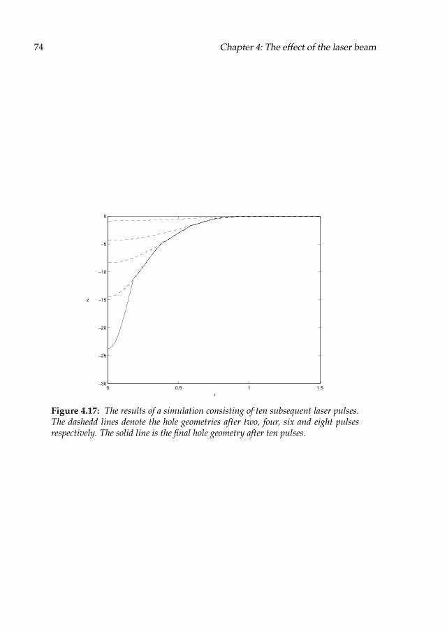
74 Chapter 4: The effect of the laser beam
0 0.5 1 1.5−30
−25
−20
−15
−10
−5
0
z
r
Figure 4.17: The results of a simulation consisting of ten subsequent laser pulses.The dashedd lines denote the hole geometries after two, four, six and eight pulsesrespectively. The solid line is the final hole geometry after ten pulses.

CHAPTER 5
Splashing and solidification
In this chapter we focus on the splashing and solidification models, briefly describedin Chapter 2. We will derive the leading-orders for these two models in Sections 5.1and 5.2. The splashing model contains a link to the model for the gas dynamicsand this model needs to be investigated further experimentally. Therefore, we willexplain a method to solve the leading-order model for solidification in Section 5.3.
5.1 Axisymmetric splashing model
In this section we derive the leading-order equations for the splashing model. Forthis we start of from the non-dimensional form of the equations describing the splash-ing mechanism as already derived in Chapter 2. These represent conservation ofmass
∂2φ
∂r2+1
r
∂φ
∂r+1
δ2∂2φ
∂z2= 0 (5.1a)
and conservation of energy
∂θ
∂t+∂φ
∂r
∂θ
∂r+1
δ2∂φ
∂z
∂θ
∂z=
D
δ2(
∂2θ
∂r2+1
r
∂θ
∂r
)
+∂2θ
∂z2
, in Ωl (5.1b)
in the liquid. Conservation of energy in the solid led to
∂θ
∂t= D
δ2(
∂2θ
∂r2+1
r
∂θ
∂r
)
+∂2θ
∂z2
, in Ωs. (5.2)
The vaporizing isotherm is expressed by
θ = θv(p). (5.3a)

76 Chapter 5: Splashing and solidification
Furthermore, we have conservation of momentum
∂φ
∂t+1
2
(
(
∂φ
∂r
)2
+1
δ2
(
∂φ
∂z
)2)
+ p = 0, (5.3b)
and conservation of energy
1
δ2∂φ
∂z−∂φ
∂r
∂h
∂r−∂h
∂t= I−
D
λvLv
(
∂θ
∂z− δ2
∂h
∂r
∂θ
∂r
)
on z = h(r, t), (5.3c)
on the vaporizing surface. The solid-liquid interface is at melting temperature
θ = 0. (5.4a)
Conservation of mass yielded
1
δ2∂φ
∂z=∂φ
∂r
∂s
∂r, (5.4b)
and the Stefan condition told us
λf∂s
∂t+D
[
∂θ
∂z− δ2
∂s
∂r
∂θ
∂r
]s+
s−
= 0 on z = s(r, t). (5.4c)
Finally, at infinity we have ambient conditions
θ → θa as z → −∞. (5.5)
We introduce expansions of the form
φ ∼ φ0 + δ2φ1, θ ∼ θ0 + δ2θ1, h ∼ h0 + δ2h1, s ∼ s0 + δ2s1, (5.6)
where φ∗, θ∗, h∗ and s∗ are independent of δ. We transfer the condition from thecorrect boundary z = s to a convenient boundary z = s0 by using a Taylor seriesexpansion, that is
∂φ
∂z
∣
∣
∣
∣
y=s
=∂φ0
∂z
∣
∣
∣
∣
z=s0
+ δ2
(
∂φ1
∂z
∣
∣
∣
∣
z=s0
+ s1∂2φ0
∂z2
∣
∣
∣
∣
z=s0
)
+O(δ4). (5.7)
A similar transfer takes place between z = h and z = h0.
Equation (5.1a) gives us
∂2φ0
∂z2= 0.
Together with (5.4b), which tells us
∂φ0
∂z= 0, at z = s0,

5.1: Axisymmetric splashing model 77
this leads to
∂φ0
∂z= 0.
Thus,
φ0 = a(r, t).
Substituting this into (5.1a) again, yields
∂2φ1
∂z2= −
∂2a
∂r2−1
r
∂a
∂r= −
1
r
∂
∂r
(
r∂a
∂r
)
,
and therefore
∂φ1
∂z= −
z
r
∂
∂r
(
r∂a
∂r
)
+ c(r, t).
Then (5.4b) gives us
∂φ1
∂z=∂a
∂r
∂s0
∂r, on z = s0.
Thus
c(r, t) =∂a
∂r
∂s0
∂r+s0
r
∂
∂r
(
r∂a
∂r
)
=1
r
∂
∂r
(
s0r∂a
∂r
)
.
So
φ1 = −z2
2r
∂
∂r
(
r∂a
∂r
)
+z
r
∂
∂r
(
s0r∂a
∂r
)
+ b(r, t).
Through this derivation, we obtain
φ ∼ a+ δ2b−
z2
2r
∂
∂r
(
r∂a
∂r
)
r
+z
r
∂
∂r
(
s0r∂a
∂r
)(5.8)
where a = a(r, t) and b = b(r, t) are unknown functions. Substituting (5.8) into (5.1b),(5.3b) and (5.3c), we find
∂θ0
∂t+∂a
∂r
∂θ0
∂r+
1
r
∂
∂r
(
r∂a
∂rs0
)
−z
r
∂
∂r
(
r∂a
∂r
)∂θ0
∂z= D
∂2θ0
∂z2,
∂a
∂t+1
2
(
∂a
∂r
)2
+ p = 0,
and
∂h0
∂t+1
r
∂
∂r
(
r∂a
∂r(h0 − s0)
)
+ I = 0,

78 Chapter 5: Splashing and solidification
respectively. Finally, we make the substitution u = ∂a∂r
, to give a differential equationfor the temperature
∂θ0
∂t+ u
∂θ0
∂r+
1
r
∂
∂r(rus0) −
z
r
∂
∂r(ru)
∂θ0
∂z
= D∂2θ0
∂z2for s0 < z < h0, (5.9)
with two boundary conditions
θ0 = 0, on z = s0 θ0 = θv(p) on z = h0, (5.10)
the equation for the evolution of the velocity
∂u
∂t+ u
∂u
∂r+∂p
∂r= 0, (5.11)
the equations for the evolution of the free boundaries
∂h0
∂t+1
r
∂
∂rru(h0 − s0) + I = 0, λf
∂s0
∂t+D
[
∂θ0
∂z
]s+
0
s−
0
= 0, (5.12)
the equation and the boundary condition for conduction in the solid
∂θ0
∂t= D
∂2θ0
∂z2for z < s0 and θ0 → θa as z → −∞. (5.13)
The leading-order equations to describe axisymmetric splashing are (5.9)-(5.13).
We rewrite this set of equations to avoid complications with subscripts in subsequentsections. Furthermore, we chose to use the film thickness ξ := h0 − s0 as a variablerather than h0. We also replace s0 by ψ and omit the subscript in θ0 in the numericalmodel. This leaves us with the following system of equations
∂ξ
∂t+1
r
∂
∂r(ruξ) = −I−
∂ψ
∂t, (5.14)
∂u
∂t+ u
∂u
∂r+∂p
∂r= 0, (5.15)
∂θ
∂t+1
r
∂
∂r(ruθ) +
∂
∂z
(1
r
∂
∂r(ruψ) −
z
r
∂
∂r(ru)
θ−D
∂θ
∂z
)
= 0, (5.16)
and
θ = θv(p) on z = ψ+ ξ, (5.17)
in the fluid,
θ = 0, (5.18)

5.2: Planar solidification model 79
and
λf∂ψ
∂t+D
[
∂θ
∂z
]ψ+
ψ−
= 0, on z = ψ, (5.19)
at the interface and
∂θ
∂t= D
∂2θ
∂z2, for z < ψ (5.20)
and
θ → θa as z → −∞, (5.21)
in the solid.
5.2 Planar solidification model
The derivation of the leading-order equations for the soldification model is similarto that of the splashing model. We use the same expansions, that is (5.6), and alsotransfer the boundary conditions using Taylor series expansions as in (5.7).
Similar to the derivation followed in the previous section, from Eqs. (2.44a) and (2.47b)we obtain
φ ∼ a+ δ2b−
1
2
∂2a
∂x2y2 +
∂
∂x
(
∂a
∂xs0
)
y
, (5.22)
where a = a(x, t) and b = b(x, t) are unknown functions. Substituting u = ∂a∂x
,we find, similarly to the derivation in the previous section, the following system ofequations:
∂ξ
∂t+∂
∂x(uξ) = −
∂ψ
∂t, (5.23)
∂u
∂t+ u
∂u
∂x= 0, (5.24)
∂θ
∂t+∂
∂x(uθ) +
∂
∂y
(∂
∂x(uψ) −
∂u
∂xy
θ−D
∂θ
∂y
)
= 0, (5.25)
and
∂θ
∂y= 0 on y = ψ+ ξ, (5.26)
in the fluid,
θ = 0, (5.27)

80 Chapter 5: Splashing and solidification
and
λf∂ψ
∂t+D
[
∂θ
∂y
]ψ+
ψ−
= 0, on y = ψ, (5.28)
at the interface and
∂θ
∂t= D
∂2θ
∂y2, for y < ψ (5.29)
and
θ → θa as y → −∞, (5.30)
in the solid.
This system of equations together with suitable initial conditions will be treated nu-merically in Section 5.3.
5.3 Numerical methods for solidification
We consider the leading-order problem for the solidification of an amount of moltenmaterial flowing past a relative cold solid wall. For its derivation, see Section 5.2.Here ξ = ξ(x, t) represents the thickness of melt film and ψ = ψ(x, t) representsthe height of the solid-liquid boundary. Furthermore θ = θ(x, y, t) represents thetemperature of the material, and u = u(x, t) represents the horizontal velocity of themelt film. Note that all the variables are dimensionless. The problem consists of thefollowing equations.
Conservation of mass
∂ξ
∂t+∂
∂x(uξ) = −
∂ψ
∂t; (5.31)
Burgers equation
∂u
∂t+ u
∂u
∂x= 0. (5.32)
The combination of these two equations also gives the conservation of momentumequation
∂
∂t(uξ) +
∂
∂x(u2ξ) = −u
∂ψ
∂t. (5.33)
Furthermore, we have conservation of energy in the melt
∂θ
∂t+∂
∂x(uθ)+
∂
∂y
(∂
∂x(uψ) −
∂u
∂xy
θ−D
∂θ
∂y
)
= 0 for ψ < y < ψ+ξ, (5.34)

5.3: Numerical methods for solidification 81
which may also be written as
∂θ
∂t+ u
∂θ
∂x+
∂
∂x(uψ) −
∂u
∂xy
∂θ
∂y−D
∂2θ
∂y2= 0 for ψ < y < ψ+ ξ. (5.35)
Furthermore, there is no heat flux through the top surface:
∂θ
∂y= 0 on y = ψ+ ξ. (5.36)
We have the Stefan condition
λf∂ψ
∂t+D
[
∂θ
∂y
]ψ+
ψ−
= 0, (5.37)
and the melting isotherm
θ = 0 on y = ψ, (5.38)
at the solid-liquid interface. The well-known heat equation holds in the solid
∂θ
∂t= D
∂2θ
∂y2for y < ψ, (5.39)
with ambient conditions at infinity
θ → θa as y → −∞. (5.40)
The initial conditions are prescribed velocity
u(x, 0) = u0(x), (5.41)
prescribed temperature
θ(x, y, 0) = θ0(x, y), (5.42)
and a prescribed geometry
ξ(x, 0) = ξ0(x), (5.43)
and
ψ(x, 0) = ψ0(x). (5.44)
Here we assume
θ0(x, y) = θa for y < ψ0(x), θ0(x,ψ0(x)) = 0 and∂θ0
∂y(x,ψ0(x) + ξ0(x)) = 0 for ξ0(x) > 0.

82 Chapter 5: Splashing and solidification
5.3.1 Shocks
We note that (5.32) uncouples from the system of equations. As known, this equa-tion can exhibit shocks, see e.g. [51]. Because the melt always has compact support,shocks will occur. Let u(x, 0) = u0(x) be the initial velocity profile. Then the time offirst ’breaking’ is
tB = −1
u ′0(Xs)
,
where Xs is defined by:
u ′0(Xs) < 0, |u ′
0(Xs)| is a maximum.
To study the shock in detail, we use that u0(x) vanishes outside the range [XL, XR],and u0(x) > 0 in the range. Then, one can show ([51, pp. 46–47]) that for t > tB theasymptotic formulas for the position of the shock s(t) and the velocity just behindthe shock u are
s ∼√2At, (5.45)
u ∼
√
2A
t, (5.46)
respectively. Here
A =
∫XR
XL
u0(x)dx (5.47)
is the area of the hump. The asymptotic form of the velocity profile is
u ∼x− XL
t, XL < x < XL +
√2At. (5.48)
So, the details of the initial velocity distribution are lost; only the areaA is preserved.
Because the shock in the velocity distribution travels at half the speed of the velocityjust behind the shock and because of conservation of mass, melt will amass behindthis leading edge shock.
5.3.2 Enthalpy Method
We define XL(t) and XU(t) to be the points XL(t) = infx|ξ(x, t) > 0 and XU(t) =
supx|ξ(x, t) > 0, that is, XL(t) and XU(t) represent the ‘beginning’ and ‘ending’ ofthe liquid blob, respectively. We introduce the dimensionless enthalpy, η, by
η =
θ θ < 0 (solid),
θ+ λf θ > 0 (liquid),(5.49)

5.3: Numerical methods for solidification 83
and therefore
θ =
η η < 0,
0 0 < η < λf,
η− λf η > λf,
(5.50)
The Eqs. (5.34)1, (5.37), (5.38) and (5.39)1 can then be rewritten as
∂η
∂t+∂
∂x(χuθ) +
∂
∂y
(
χ
∂
∂x(uψ) −
∂u
∂xy
θ
)
−D∂2θ
∂y2= 0, (5.51)
where χ is the characteristic function
χ =
0 θ < 0 (solid),
1 θ > 0 (liquid).(5.52)
Alternatively, (5.51) can be written as
∂η
∂t+ χu
∂θ
∂x+ χ
∂
∂x(uψ) −
∂u
∂xy
∂θ
∂y−D
∂2θ
∂y2= 0. (5.53)
We will use this enthalpy method in our numerical method as will be explained inthe next section.
5.3.3 Numerical Method
The geometry that will be used throughout this section is sketched in Figure 5.1. The
(*)
( +
( ,.- /0
( 1
2
3
45- /0
Figure 5.1: The geometry used in the numerics for the solidification problem.
problem to solve is comprised by (5.31), (5.33) or (5.32), and (5.51) together with therelationships between temperature and enthalpy (5.49) and (5.50) and the boundaryand initial conditions (5.36) and (5.40)-(5.44).
One way of solving this system is the following. Suppose everything is known attime level tn: En, θn, un, ξn, ψn, Ωn. From the enthalpy equation (5.51) togetherwith (5.49) and (5.50), we find En+1, θn+1 and ψn+1. Now we’ve got a choice: we

84 Chapter 5: Splashing and solidification
PSfrag replacements E θ ψ u ξ
En θn ψn un ξn
En+1 θn+1 ψn+1 un+1 ξn+1
Limiter
SLMSLM
Burgers
Heat
Mass
Spline
Figure 5.2: The numerical scheme.
could use the coupled system (5.31) and (5.33) to compute un+1 and ξn+1 or wecould use (5.31) and (5.32) for this. The latter method has the benefit that this is adecoupled system, un+1 follows from (5.32) and ξn+1 then follows from (5.31). Thefinal step is then to compute the new domainΩn+1 from un+1, ξn+1 andψn+1. Thisnumerical solving procedure is depicted in Figure 5.2. As un represents a vectorof velocities on different coordinates, we cannot use this vector as such in the 2Denthalpy problem. Hence, the ’Spline’-block in this figure represents a possible wayof dealing with this.
The slope limiter scheme
In order to solve Burgers’ equation for the horizontal velocity we use a slope limitermethod, see e.g. [26]. This slope limiter method is based on the Godunov scheme andis therefore a finite volume method. Consider the following initial value problem foru(x, t)
∂u
∂t+∂f(u)
∂x= 0, x ∈ R, t > 0, (5.54a)
u(x, 0) = u(x), x ∈ R. (5.54b)

5.3: Numerical methods for solidification 85
We introduce control volumes Vj:
Vj :=[
xj− 12, xj+ 1
2
)
, xj+ 12
=1
2(xj + xj+1) , j = 0,±1,±2, . . . (5.55)
The numerical solution unj has to be interpreted as an approximation of the aver-age value of u(x, t) over Vj at time level tn. Associated with this unj we define thefunction U(x, t) by:
∂U
∂t+∂f(U)
∂x= 0, x ∈ R, t > tn, (5.56a)
U(x, tn) = unj + snj (x− xj), x ∈ Vj, j = 0,±1,±2, . . . , n = 0, 1, 2, . . .
(5.56b)
Here, unj and snj are the average value and slope, respectively, of U(x, tn) in thecontrol volume Vj. The ‘initial’ valueU(x, tn) is thus piecewise linear in each Vj. Theslope snj is still unknown, and has to be determined such that the resulting schemeis Total Variation Diminishing (TVD), see e.g [20]. The slope limiter method is basedon the integral formulation of the initial value problem (5.56).
After integration over the control volume Vj and over the time interval [tn, tn+1], weobtain
∫
Vj
U(x, tn+1)dx−
∫
Vj
U(x, tn)dx = −∆t(
F(unj , unj+1) − F(unj−1, u
nj ))
, (5.57)
where the numerical flux F(unj , unj+1) is defined as
F(unj , unj+1) :=
1
∆t
∫ tn+1
tn
f(U(xj+ 12, t))dt. (5.58)
To compute the numerical flux F(unj , unj+1) we have to solve the generalized Rie-
mann problem comprised by the conservation law (5.56a) and the piecewise linearinitial condition. This is generally difficult and involving, and for that reason wereplace the flux f(u) by its linear interpolant f(u), i.e.
f(u) := f(unj ) + anj+ 1
2
(u− unj ), u ∈ int(unj , unj+1), (5.59)
with anj+ 1
2
the finite difference approximation of f ′(u(xj+ 12, tn)) given by
anj+ 1
2
:=
f(un
j+1)−f(unj )
unj+1
−unj
if unj 6= unj+1,
0 if unj = unj+1.(5.60)
Replacing f(u) by f(u), the generalized Riemann problem reduces to the followinginitial value problem
∂U
∂t+ an
j+ 12
∂U
∂x= 0, x ∈ R, t > tn, (5.61a)
U(x, tn) = unj + snj (x− xj), x ∈ Vj, j = 0,±1,±2, . . . , n = 0, 1, 2, . . .
(5.61b)

86 Chapter 5: Splashing and solidification
Analoguous to (5.58), the numerical flux F(unj , unj+1) is the time average of f(U(xj+ 1
2, t))
over [tn, tn+1], i.e.
F(unj , unj+1) =
1
∆t
∫ tn+1
tn
f(U(xj+ 12, t))dt. (5.62)
The computation of U(xj+ 12, t) from (5.61b) is straightforward, and, provided that
anj+ 1
2
> 0, we obtain
U(xj+ 12, t) = unj + snj
(
1
2∆x− an
j+ 12
(t− tn)
)
, (5.63)
and subsequently substituting this expression into (5.62), we find for the numericalflux
F(unj , unj+1) = f(unj ) +
1
2anj+ 1
2
(
1−∆t
∆xanj+ 1
2
)
∆xsnj . (5.64)
Finally, we have to determine slopes snj such that the resulting scheme is TVD. Wedo this using the technique of slope limiters. We take
snj = Φnj+ 1
2
1
∆x(unj+1 − unj ), (5.65)
where Φnj+ 1
2
is a limiter on the slope (unj+1 − unj )/∆x. Usually the limiter Φnj+ 1
2
isgiven by
Φnj+ 1
2
= Φ(rnj+ 1
2
), (5.66)
with Φ(r) the so-called limiter function and where rnj+ 1
2
is defined by
rnj+ 1
2
:=unj − unj−1
unj+1 − unj, (5.67)
provided that anj+ 1
2
> 0. More about these limiter functions can be found at the endof this section.
Finally, the numerical value un+1j is defined as the average value of U(x, tn+1) over
Vj, i.e.
un+1j :=
1
∆x
∫
Vj
U(x, tn+1)dx. (5.68)
Substituting (5.68) into (5.57) leads to the final scheme
un+1j = unj −
∆t
∆x(F(unj , u
nj+1) − F(unj−1, u
nj )), (5.69)
with the numerical flux F(unj , unj+1) as in (5.64).

5.3: Numerical methods for solidification 87
We conclude this derivation with mentioning three limiter functions. A smooth lim-iter function is due to Van Leer [46], and is given by
Φ(r) =2r
1+ r, (5.70)
for r > 0. Another limiter function, especially suited for representing discontinuities,is the so-called superbee limiter function of Roe [35]. It is given by
Φ(r) = max(min(1, 2r),min(r, 2)), (5.71)
for r > 0. The last limiter function we mention here is called the minmod limiterfunction (see [26]) and is given by
Φ(r) = max(0,min(1, r)). (5.72)
An elaborated example
We take the case of no solidification as an example. That is, we only look at themovement of the liquid blob. We use Eqs. (5.31) and (5.32) without the solidificationterm ∂ψ
∂t, i.e.
∂ξ
∂t+∂(uξ)
∂x= 0, (5.73a)
and
∂u
∂t+∂(12u2)
∂x= 0. (5.73b)
The initial conditions to go with these equations are prescribed geometry and a pre-scribed velocity
ξ(x, 0) = ξ(x), u(x, 0) = u(x). (5.74)
Eqs. (5.73) are both in the form as in (5.54) and we therefore use the slope limitermethod on both equations to solve this.
Burgers’ equation
Following the derivation of the slope limiter scheme as in the previous section withf(u) = 1
2u2 we get the scheme
un+1j = unj −
∆t
∆x(F(unj , u
nj+1) − F(unj−1, u
nj )), (5.75)
with numerical flux F(unj , unj+1) given by
F(unj , unj+1) =
1
2(unj )2 +
1
2anj+ 1
2
(
1−∆t
∆xanj+ 1
2
)
∆xsnj , (5.76)

88 Chapter 5: Splashing and solidification
where
anj+ 1
2
=
12
(
(unj+1)2 − (unj )2
)
unj+1 − unj=1
2(unj+1 + unj ). (5.77)
We can employ this scheme starting from the known initial velocity distributionu(x, 0) = u(x).
Mass balance
For the mass balance equation (5.73a) we get the scheme
ξnj+1 = ξnj −∆t
∆x(F(ξnj , ξ
nj+1) − F(ξnj−1, ξ
nj )), (5.78)
with numerical flux F(ξnj , ξnj+1) given by
F(ξnj , ξnj+1) = unj ξ
nj +
1
2anj+ 1
2
(
1−∆t
∆xanj+ 1
2
)
∆xsnj , (5.79)
where
anj+ 1
2
= unj+ 1
2
. (5.80)
The numerical scheme for this elaborated example is depicted in Figure 5.3.
ResultsThe analytical results for this system of equations as stated in Section 5.3.1 are clearlyvisible in the numerical results. We see the asymptotic triangular profile of the ve-locity distributions and the corresponding melt accumulation at the leading edgeshock.
We will use the finite element method for solving the heat equation (5.53)
∂η
∂t+ χu
∂θ
∂x+ χ
∂
∂x(uψ) −
∂u
∂xy
∂θ
∂y−D
∂2θ
∂y2= 0, (5.81)
together with the no flux boundary condition on temperature (5.36), ambient condi-tions at infinity (5.40) and the initial condition (5.42). Furthermore the relationshipbetween the enthalpy η and the temperature θ is described by (5.49) and (5.50).
We search for a weak solution of (5.81). Multiply (5.81) with a weight function pwhich vanishes on Γ1 and integrate over the domain. Using the divergence theoremwe get the finite element variational formulation
∫
Ω
∂η
∂tp+ χup
∂θ
∂x+ χ
∂
∂x(uψ) −
∂u
∂xy
p∂θ
∂y+D
∂p
∂y
∂θ
∂ydσ =
∫
Γ
Dp∂θ
∂ynyds = 0 for all p ∈ H10. (5.82)

5.3: Numerical methods for solidification 89
PSfrag replacements
u ξ
un ξn
un+1 ξn+1
Limiter
SLMSLM
Burgers Mass
Figure 5.3: The numerical scheme for the elaborated example. The dashed boxstands for the loop.
Here the last equality comes from the boundary condition of θ on Γ3 (5.36) and thefact that p|Γ1
≡ 0.
Next, we consider a finite element discretization of Ω with a finite element spaceVh ⊂ H10(Ω) spanned by the basis ϕi
Ni=1. A typical choice for the basis functions
would be the hat functions. We look for finite element solutions
η(x, t) = ηΓ1 + ηΩ\Γ1 = ηΓ1 +
N∑
i=1
ηi(t)ϕi(x) (5.83)
and
θ(x, t) = θΓ1 + θΩ\Γ1 = θΓ1 +
N∑
i=1
θi(t)ϕi(x). (5.84)
The superscript Γ1 is used to indicate that the inhomogeneous Dirichlet boundaryconditions at Γ1 are fulfilled by this term.

90 Chapter 5: Splashing and solidification
0 0.5 1 1.5 2 2.5 3 3.5 4 4.5 5−0.2
0
0.2
0.4
0.6
0.8
1
1.2
Figure 5.4: The evolution of the velocity profile
0 0.5 1 1.5 2 2.5 3 3.5 4 4.5 5
0
0.5
1
1.5
2
2.5
3
3.5
Figure 5.5: The evolution of the melt drop
The computational problem is to determine the time dependent coefficients ηi(t)and θi(t) for i = 1, . . . ,N. Substituting the approximations into the variational for-mulation and taking the weight functions to be the basis functions ϕj, j = 1, . . . ,N
we obtain the set of equations in matrix form
Mdη
dt+ C(u,ψ)θ +DSθ = b. (5.85)
We use the bold face characters for matrices and vectors. So, η = [ηi(t)] and θ =
[θi(t)]. The mass matrix M, the convection matrix C, the stiffness matrix S and theright-hand side b are defined as follows:
[M]ij =
∫
Ω
ϕiϕjdσ, (5.86a)
[C]ij =
∫
Ω
χuϕi∂ϕj
∂x+ χ
∂
∂x(uψ) −
∂u
∂xy
ϕi∂ϕj
∂ydσ, (5.86b)

5.3: Numerical methods for solidification 91
[S]ij =
∫
Ω
∂ϕi
∂y
∂ϕj
∂ydσ, (5.86c)
[b]i = −
∫
Ω
χuϕi∂θΓ1
∂x+ χ
∂
∂x(uψ) −
∂u
∂xy
ϕi∂θΓ1
∂y+D
∂θΓ1
∂y
∂ϕi
∂ydσ. (5.86d)
Together with the initial conditions on temperature (5.42) and hence via the relation-ship also on enthalpy, we have a set of initial value problems which can be solvednumerically.
In order to show how we solve (5.85) by the ϑ-method, we rewrite it as
Mdη
dt= FFF(u,ψ,η, t) := b − C(u,ψ)θ(η) −DSθ(η). (5.87)
Suppose everything is known at t = tk. The enthalpy distribution and temperaturedistributions in the material at time t = tk+1 are then computed by the ϑ-method.We obtain
GGG(ηk+1) := M(ηk+1 − ηk)
− ∆t(
ϑFFF(uk+1, ψk+1,ηk+1, tk+1) + (1− ϑ)FFF(uk, ψk,ηk, tk))
= 0. (5.88)
In order to solve (5.88) for ϑ 6= 0, the occurence of ηk+1 does not cause problems;this could be dealt with in a similar way as in the melting model, see the previouschapter. The problem for ϑ 6= 0 lies in the ψk+1 and uk+1 terms.
For ϑ = 0 the procedure is simply the following. Compute the enthalpy distributionin the material at time t = tk+1 via
Mηk+1 = Mηk + ∆tFFF(uk, ψk,ηk, tk), (5.89)
and then update the temperature via (5.49) to get
θk+1i = θ(ηk+1
i ). (5.90)
The position of the solid-liquid boundary ψ at time level t = tk+1 is simply themelting isotherm.
For ϑ 6= 0 we can use a quasi Newton method. That is, we freeze the u and ψ terms
GGG(ηk+1) := M(ηk+1−ηk)−∆t(ϑFFF(uk, ψk,ηk+1, tk+1)+(1−ϑ)FFF(uk, ψk,ηk, tk)) = 0.
(5.91)
The iteration to obtain the solution at t = tk+1 is as follows
ηk+1,l = ηk+1,l−1 − (∂GGG(ηk+1,l−1))−1GGG(ηk+1,l−1), l = 1, 2, . . . ,
ηk+1,0 = ηk.
(5.92)

92 Chapter 5: Splashing and solidification
This is similar to the method used in the previous chapter in solving the enthalpyproblem for laser induced melting. The difference lies in the operator GGG. Here, theJacobian ∂GGG(η) is given by
∂GGG(ηk+1,∗) = M + ∆tϑ(C(uk, ψk) −DS)∂θ
∂η(ηk+1,∗). (5.93)
The iteration in (5.92) is stopped when a given accuracy is reached.
After one complete time step for both the enthalpy problem and the two slope limiterschemes has been calculated, we will need to adapt the domain of computation. Onehas to be aware of the fact that as the liquid moves and the solid obviously does not,interpolating the old solution on the new domain is a point of attention.

CHAPTER 6
Computational platforms
In the numerical procedures outlined in the previous chapters, several solution al-gorithms are used. Each algorithm consists of a sequence of operations on specificdata. Most of these operations are available as part of public domain or commerciallibraries (collections of operations) or as operating system commands. However, dif-ferent libraries tend to use different data structures and most computational librarieswere not written with visualization in mind. The same holds for the visualization ofthe results, which is a very important aspect in simulation. Several user friendly andextensive libraries for visualization are available. Preferably we want to use these ex-isting and often well documented libraries together. This chapter shows how this isachieved by adorning existing libraries with an interface within the NumLab visualprogramming environment (see [28]). Section 6.1 shows how the to be introducedinterface can be used to implement complex numerical algorithms in a convenientmanner. The setup of such an interface is treated in Section 6.2 using the example ofthe Piecewise Polynomial Package, PPPack [10].
6.1 Scientific computing
The focus for the implementation of complex numerical algorithms must be on thereuse of existing unaltered libraries. Most libraries use own (i.e. non-standard) datastructures so that they cannot be used jointly. Therefore, these libraries do not seemto aid to the implementation of complex numerical problems. In order to use li-braries within a broader framework, these libraries need to communicate with eachother in some way. Basically, a library is a collection of operations on a specificdata type and normally different libraries use different data types. Within the Num-Lab visual programming environment communication between different librariesis achieved by equiping all ”outside” libraries with an interface ensuring that thelibrary accepts the same (common) data type, as depicted in Fig. 6.1 for the solidifi-cation problem of Section 5.3. The outer circles denote the used existing ”outside”

94 Chapter 6: Computational platforms
libraries, the grey shells denoting their interfaces. The arrows denote the data flowbetween the libraries and the solidification program. The inner circle is the numeri-cal solution procedure for the solidification problem encoded within NumLab. The
solidificationproblem
in-house
PPPack
LAPackSEPRAN
VTK
OI
Figure 6.1: Schematic overview of the numerical procedure of the solidificationproblem within NumLab.
transformation of the generic NumLab data type to the library specific data type isprovided within the library interface. This interface provides additional functional-ity, see [13], which is beyond the scope of this thesis. The interface enables us to usethe existing libraries in an unaltered way and, furthermore, within a visual program-ming environment.
For each of the solidification’s subproblems, numerical solution procedures exist.Thus, the problem can be solved with a combination of the operations, which residein different libraries, as shown in Fig. 6.1. The finite element package SEPRAN [37]builds the system of equations resulting from the finite element formulation of theproblem, see Section 5.3. The Linear Algebra Package LAPack [2] routines are thenused to solve the system. On the other hand, the solid-liquid interface as well as thesurface are represented by smooth splines using the Piecewise Polynomial PackagePPPack [10] and the positions of these moving boundaries are calculated using in-house written finite volume codes, see Section 5.3. The results are visualized using

6.1: Scientific computing 95
the Visualization ToolKit (VTK) [36] and Open Inventor (OI) [50] libraries. The needfor some sort of communication between these different packages and libraries isobvious.
1
2
3
Figure 6.2: The program which solves a part of the solidification problem andvisualizes the output.
Figure 6.2 shows the implementation of the problem described by Eq. (5.73) as de-rived in Section 5.3, loaded into the NumLab visual programming environment,see [28]. The implementation uses modules (we use the word module for both oper-ations and data structures) from different libraries including LAPack, PPPack, VTK,OI, etc., as well as operating system commands: the mpeg module. Most numericalprograms, like the one in Fig. 6.2, can be divided into three parts:

96 Chapter 6: Computational platforms
1. the part which reads the input and performs the numerical computations,
2. the part which visualizes the computed results and
3. the post-processing part which writes the output.
Figure 6.2 needs further explanation. Each rectangle such as MIteration is a graph-ical representation of an operation belonging to a certain library. For the sake of con-venience, this representation is also called a module. Within each module, we discerna bottom and a top area. Modules may have both input and output arguments. Eachof its arguments made available via the interface description, is mapped onto a smallcoloured rectangular area at the bottom or top of the module, the input argumentsbeing related to the top, the output arguments to the bottom. These small rectangu-lar regions are called ports. Different built-in data types are coloured in a differentmanner, all pointers and derived types are coloured using a default. Each port iseither connected, or behind the scenes a default value is used. Output is connectedto input using the mouse by clicking on the bottom output port, dragging to the topinput port and releasing. The connection is established when the data types concur,and refused when this is not the case. Default values can be altered using a graphicaluser interface, called the interactor (Fig. 6.3), which is automatically generated fromthe function’s interface, and which pops up when selected. This automatically builteditor can be used to enter the values of arguments which are not connected. As
Figure 6.3: The user provides default values to the modules using an automati-cally built editor.
an example, see Fig. 6.3, which shows the equivalent of the Matlab linspace func-tionality. We can prescribe an interval [a, b] ⊂ R and a number of points n ∈ N
and the module generates a vector z ∈ Rn of n points linearly spaced between, and
including, a and b, as well as the spacing h.
Figure 6.4 depicts a VTK Viewer, belonging to a VTK Viewer module, which showsthe initial shape of the melt blob flowing along the walls, superimposed with graph-

6.2: Example 97
ical operations onto the inside of a cylinder wall. This VTK viewer as well as theOI viewer offers solid, hidden-line, wire-frame and other representations, as well asinteractive 3D manipulation of the visualized objects.
Figure 6.4: Visualization of the solidification process.
Building complex numerical algorithms with NumLab is convenient because of anumber of reasons. Firstly, the libraries LAPack, EigPack, SEPRAN, PPPack, VTK,OI, etc. have been interfaced and can therefore be used together without restrictionsand explicit user data type conversions. In the example discussed in this section,we used SEPRAN and PPPack to build the equations, LAPack to solve them andVTK to visualize the results. Secondly, several methods have been added to theNumLab computational platform, like new data-types, data-exchange in MATLAB /Mathematica / Open-Math / LaTeX / VTK / other formats, and discretized ordinaryand partial differential related operators. Furthermore, programming in a visualenvironment aids to the reusability of complex numerical algorithms.
6.2 Example
For this NumLab environment as sketched above, we show how to interface an ex-isting library. For a more thorough explanation of this technique, see [27] and ref-erences therein. Interfacing a library means interfacing all operations to be exposedfor usage. In this example we show how to interface the PPPack [10] to generatean interpolating cubic spline (see e.g. [11]). The language in which the interface is

98 Chapter 6: Computational platforms
Function Descriptiondcubspl computes polynomial coefficients of cubic splinedppvalu computes function or derivative value of cubic splinedinterv function used in dppvalu
Table 6.1: The operations from the PPPack library needed for NumLab spline operations.
implemented is C++, for reasons that are outlined in [27]. The interface consists ofthree layers, the source-layer, the class-layer and the module-layer.
The source-layer contains the operations from the libraries which the user wants touse, i.e. it is closest to the ”white” inner region of the library in Fig. 6.1. For the cubicspline, these are given in Table 6.1. The dcubspl routine computes the polynomialcoefficients describing the interpolating cubic spline and writes these to a matrixC. For this it basically needs three groups of input, the first and second being theabscissae and ordinates of the data points, respectively, and the third describing theboundary conditions in terms of type and value. Once the spline has been built, itsfunction or derivative value at a point x can be computed from the matrix C usingthe dppvalu routine. The dinterv routine is merely an operation used repeatedlywithin dppvalu. Because Fortran generates function names according to a differentrule than C++, we need to provide each Fortran function we want to use within ourC++-interface with a shell that ensures that the Fortran function is called.
The class-layer contains the C++ class version of a cubic spline. Its constructor callsback to the dcubspl routine in the source-layer and checks whether this went cor-rectly. The function value or j-th derivative value of the cubic spline can be ob-tained using the operator(). If spline is an instance of the spline class, thenspline(x) and spline(x,j) return the function value and the value of the j-thderivative of the spline in point x, respectively. This operator() calls back to thedppvalu routine.
Finally, the module-layer contains a class. This so called module delegates all oper-ations to the class-level and, moreover, is adorned with a few standard data-flowoperations for use in a visual programming environment. This module-layer makesthe spline class accessible within a visual programming environment through thegraphical representation as depicted in Fig. 6.5. This module has eight ports on the
Figure 6.5: The spline module. Please consult the text for further explanaition.

6.2: Example 99
top and two at the bottom. The first port on both the top À and the bottom È is apointer to the instance of the class itself. The other top ports represent the input ar-guments: the point x at which the spline should be evaluated Á, the abscissae  andordinates à of the data points and the type and value of the left (Ä and Å) and right(Æ and Ç) boundary conditions. The second port at the bottom É is the functionvalue of the cubic interpolating spline at point x.
Figure 6.6 shows a network in which a spline through three data points is generated.The boundary conditions used to generate the cubic spline are shown in the interac-tor. This interactor also shows the benefit visual programming environments haveover non-graphical ones: all required input data is shown in a clear way. The typeof boundary condition is chosen through a pull-down menu with enumeratic typeswith descriptive names such as Dx converted to an integer for the Fortran routinedcubspl, which needs an integer describing the type. The resulting spline is visual-ized using the MDFxSampler module, which input arguments are a function, in thiscase the cubic spline function, and a vector, in this case a uniform gridding of the in-terval [−1, 1]. The output of the sampler module is a vector containing the functionvalues at these abscissae. These two vectors can be visualized using VTK operationsresulting in the VTK Viewer window as shown in the figure.

100 Chapter 6: Computational platforms
Figure 6.6: The spline module within a network.

CHAPTER 7
Conclusions andRecommendations
Numerous experiments show that most of the material removed during a laser per-cussion drilling process is in liquid state. This observation leads to the conclusionthat modelling laser induced melting is essential in a thorough understanding of thedrilling process. In this thesis the melting is investigated intensively and, moreover,also the resolidification of this molten material during splashing is studied. One ofthe main conclusions of this thesis is that the melting model reveals a small time scalein which the material reaches vaporisation temperature. Taking the scales for the gasdynamics and the splashing into consideration, multiple cycles of heating-splashingper pulse may be expected. The number of cycles per pulse depends on materialproperties and laser settings. Furthermore, the velocities for the expelled melt pre-dicted from a simplified gas dynamics model are already in good agreement withobservations.
From the analysis of the two mathematical formulations of melting investigated inthis thesis, it follows that the enthalpy method is far more suitable for more dimen-sional problems. Due to the fact that tracking the solid-liquid interface is an essentialpart of the formulation that makes use of the Stefan condition, this poses severe prob-lems in implementation for more-dimensional problems. Moreover, the enthalpymethod is also more suited for one-dimensional methods when initially only one ofthe phases is present. The main advantage of the enthalpy method over the methodemploying the Stefan condition is that the position of the interface is known a pos-teriori; it is merely an isotherm. Although this enthalpy method is known since theearly eighties we did not find papers concerning modelling of the laser drilling pro-cess that use this method.
The understanding of the incoupling of energy is essential in modelling laser per-cussion drilling. The total amount of energy absorbed by the material is the key

102 Chapter 7: Conclusions and Recommendations
parameter in the process. The incoupling of energy is governed by the reflectivity be-haviour of the material under irradiation. However, most publications on modellingthe laser-drilling process either do not use a reflection model or use an oversimpli-fied reflection model. In this thesis we use the Algebraic Ray Trace Method (ARTM)to give the actual incoupling of laser energy into the material. This reflectivity modeleasily explains the role the wavelength of the laser has on the outcome of the pro-cess, e.g. a different wavelength can easily increase the incoupling of laser energyfrom only 5% to over 50%. It is therefore obvious, that the optical behaviour of thematerial should be investigated thoroughly to get a more efficient laser drilling pro-cess. Furthermore, the reflection model easily explaines both tapering of holes dueto reflections of steep sides and better incoupling of energy in deeper holes.
Using the results of the reflection model as input of the laser-induced melting modela relatively simple simulation model has been built. By this simulation model onecan investigate the influence of different laser settings to the process. These lasersettings do not have to be conform to existing laser settings. Indeed, one can try tofind the optimal laser together with its settings for a specific desirable result. Insteadof expensive testing, one can thus get a better understanding of the role of the variouslaser parameters.
The solidification model derived in this thesis tells us that a shock may be expectedwithin the melt flowing along the relatively cold sides. This study explains whyexperimentally observed local clumps of resolidified material may arise in the drilledhole during the laser percussion drilling process. With reliable experimental andmaterial data, it may even predict a typical length at which such a clump can beexpected. The versatility of the model is shown by the fact that with only a fewmodifications the solidification model can also be used to predict the solidificationof a lava flow.
Another conclusion that can be drawn from this thesis is that it is very helpful touse existing and unaltered libraries to implement complex numerical algorithms.The software package NumLab is very instrumental in this and, moreover, offersthis within a visual programming environment thereby enhancing the reuseabilityas well as the user-friendliness of the program. To be able to use ”outside” librariesin an unaltered way, these libraries are equiped with an interface in which, amongstothers, the translation of the NumLab datatype to the library-own datatype and viceversa is provided.
Evidently, because of the complexity of the process, although many phenomena aretreated in this thesis, a simulation model will never be covering all aspects. How-ever, we will make some recommendations to enhance the modelling of laser per-cussion drilling in the following. A first recommendation is based upon an assump-tion made in the beginning of this thesis. From a computational point of view wehave restricted ourselves to axisymmetric geometries. However, the pumping for aNd:YAG laser is done by flash lamps. In this process the medium is heated up con-siderably and because of thermal effects beam distortions become serious. Becauseof a non-axisymmetric lay-out of the laser the thermal effects lead to a non-Gaussian

103
laser beam. This beam is essentially non-axisymmetric and therefore computationsshould be performed on a three-dimensional mesh to get better results.
The splashing mechanism is an extremely interesting and complex subject on itself. Itwas beyond the scope of this thesis to study this subject into all its details. However,a thorough study is needed to get a full understanding of the process of recasting.For this, experiments would be needed to acquire qualitative and quantitative in-formation about the behaviour of the material under consideration in all its phases.This last remark also leads to a third and final recommendation. We have neglectedthe absorption of laser energy by the vapour cloud for laser settings in the range westudied. However, as lasers are becoming more and more powerful energy sources,in the near future it may very well be not negligible any more for industrial lasers.A thorough understanding of this absorption is needed and furthermore, a plasmamay even be used to achieve a better incoupling of energy into the material. TheARTM will prove to be an instrumental tool for this, because, in contrast to normalray trace methods, absorption of energy within the medium can be incorporated intothe model easily. In fact, it was derived to do just that for radiation in glass.


Bibliography
[1] M. von Allmen and A. Blatter. Laser-beam interactions with materials. Springer-Verlag, 1995.
[2] E. Anderson, Z. Bai, C. Bischof, et al. LAPACK user’s guide. SIAM Philadelphia,1995.
[3] S. Anisimov. Vaporization of metal absorbing laser radiation. Soviet PhysicsJETP, 27:182–183, 1968.
[4] N.S. Asaithambi. A Galerkin method for Stefan problems. Appl. Math. Comp.,52:239–250, 1992.
[5] M. Born and E. Wolf. Priciples of optics. Pergamon Press, fifth edition, 1975.
[6] J. Crank. Free and moving boundary problems. Clarendon Press, 1984.
[7] A.J. Dalhuijsen and A. Segal. Comparison of finite element techniques for so-lidification problems. Internat. J. Numer. Methods Engrg., 23:1807–1829, 1986.
[8] B.N. Datta. Numerical linear algebra and applications. Brooks/Cole, 1995.
[9] G. Davies, editor. Properties and Growth of Diamond. Number 9 in EMIS Datare-view series. INSPEC, 1994.
[10] C. de Boor. Piecewise polynomial package. http://www.netlib.org/pppack.
[11] C. de Boor. A practical guide to splines. Number 27 in Applied MathematicalSciences. Springer-Verlag, 1978.
[12] J. Dowden, M. Davis, and P. Kapadia. Some aspects of fluid mechanics of laserwelding. J. Fluid Mech., 126:123–146, 1983.
[13] W. Drenth. A platform for numerical computations with special application to precon-ditioners. PhD thesis, Eindhoven University of Technology, to appear 2003.
[14] W.G. Driscoll and W. Vaughn, editors. Handbook of Optics. McGraw-Hill, NewYork, 1978. pp. 10-9–10-10.

106 Bibliography
[15] C.M. Elliot and J.R. Ockendon. Weak and variational methods for moving boundaryproblems. Research notes in mathematics. Pitman, 1981.
[16] J.E. Field, editor. The Properties of Diamond. Academic Press, London, 1979.
[17] M.C. Fowler and D.C. Smith. Ignition and maintenance of subsonic plasmawaves in atmospheric pressure air by CW CO2 laser radiation and their effecton laser beam propagation. J. Appl. Phys., 46:138–150, 1975.
[18] R.K. Ganesh and A. Faghri. A generalized thermal modeling for laser drillingprocess–I. Mathematical modeling and numerical methodology. InternationalJournal of Heat Mass Transfer, 40(14):3351–3360, 1997.
[19] R.K. Ganesh and A. Faghri. A generalized thermal modeling for laser drillingprocess–II. Numerical simulation and results. International Journal of Heat MassTransfer, 40(14):3361–3373, 1997.
[20] A. Harten. High resolution schemes for hyperbolic conservation laws. J. Com-put. Phys., 49:357–393, 1983.
[21] E. Hecht. Optics. Addison-Wesley, 1998.
[22] H. Ki, P.S. Mohanty, and J. Mazumder. Multiple reflection and its influence onkeyhole evolution. Journal of laser applications, pages 39–45, 2002.
[23] C.J. Knight. Theoretical modeling of rapid surface vaporization with back pres-sure. AIAA Journal, 17(5):519–523, 1979.
[24] L.D. Landau and E.M. Lifschnitz. Statistical Mechanics. Pergamon, New York,1980.
[25] H.W. Liepmann and A. Roshko. Elements of gasdynamics. John Wiley & Sons,inc., 1960.
[26] R.M.M. Mattheij, S.W. Rienstra, and J.H.M ten Thije Boonkkamp. Partial differ-ential equations Modelling, Analysis, Computing. SIAM, Philadelphia, to appear in2003.
[27] J. Maubach and W. Drenth. Data-flow oriented visual programming libraries forscientific computing. Rana 01-30, Eindhoven University of Technology, 2001.
[28] J. Maubach and A. Telea. The NUMLAB numerical laboratory for computationand visualisation. Computing and Visualization in Science, 2001. accepted.
[29] M. Mori. The finite element method and its applications. Macmillan publishingcompany, New York, 1986.
[30] M.J. Noot. Numerical analysis of turbine blade cooling ducts. PhD thesis, EindhovenUniversity of Technology, 1997.
[31] H. Ockendon and A.B. Tayler. Inviscid fluid flows. Springer-Verlag, 1983.
[32] E.D. Palik, editor. Handbook of optical constants of solids. Academic Press, NewYork, 1998.
Bibliography 107
[33] P.D. Patel. Interface conditions in heat-conduction problems with change ofphase. AIAA Journal, 6:2454, 1968.
[34] K. Raznjevic. Handbook of thermodynamic tables and charts. McGraw-Hill, 1976.
[35] P.L. Roe. Some contributions to the modeling of discontinuous flows. Lect. NotesAppl. Math., 22:163–193, 1985.
[36] W. Schroeder, K. Martin, and B. Lorensen. The visualization toolkit: an onject-oriented approach to 3D graphics. Prentice Hall, 1995.
[37] G. Segal. The SEPRAN finite element package.http://ta.twi.tudelft.nl/sepran/sepran.html.
[38] R. Siegel and J.R. Howell. Thermal radiation heat transfer. Taylor & Francis, thirdedition, 1992.
[39] A.E. Siegman. An introduction to lasers and masers. McGraw-Hill, 1971.
[40] A.E. Siegman. Lasers. Oxford University Press, 1986.
[41] W.R. Smith. Models for solidification and spalshing in laser percussion drilling.Rana 00-09, Eindhoven University of Technology, 2000.
[42] W.M. Steen. Laser material processing. Springer-Verlag, 1991.
[43] J. Stefan. Uber die Theorie der Eisbildung, insbesondere uber die Eisbildung imPolarmeere. Annalen der Physik und Chemie, 42:269, 1891.
[44] K.H. Tacke. Discretization of the explicit enthalpy method for planar phasechange. Internat. J. Numer. Methods Engrg., 21:543–554, 1985.
[45] Bas J. van der Linden. The algebraic ray trace method. PhD thesis, EindhovenUniversity of Technology, 2002.
[46] B. van Leer. Towards the ultimate conservative difference scheme ii. monotonic-ity and conservation combined in a second order accurate scheme. J. Comput.Phys., 14:361–370, 1974.
[47] J.C.J. Verhoeven. Modelling of a laser percussion drilling process. Master’sthesis, Eindhoven University of Technology, 1998.
[48] V. Voller and M. Cross. Accurate solutions of moving boundary problems us-ing the enthalpy method. International Journal of Heat Mass Transfer, 24:545–556,1981.
[49] V. Voller and M. Cross. An explicit method to track a moving phase changefront. International Journal of Heat Mass Transfer, 26:147–150, 1983.
[50] J. Wernecke. The inventor mentor: programming object-oriented 3D graphics withOpen Inventor. Addison-Wesley, 1993.
[51] G.B. Whitham. Linear and Nonlinear Waves. John Wiley, New York, 1974.
[52] M. Zerroukat and C.R. Chatwin. Computational Moving Boundary Problems. Ap-plied and Engineering Mathematics Series 8. John Wiley, New York, 1994.


Index
airfoil, 1algebraic ray trace method, see ARTMamplitude reflection coefficient, 53ARTM, 51, 56–60
barreling, 7bellow shape, 7blade, 2Brinkman number, 23
channeling, 55class-layer, 98Clausius-Clapeyron equation, 20
discrete ordinate method, see DOMDOM, 57dross, 7
effective indicesmethod of –, 54
enthalpy, 33problem, 31, 33–35, 41–43
evanescent wave, 53extinction coefficient, 52
fan, 1Fresnel equations, 53Froude number, 23
index of refractioncomplex –, 52simple –, 52
interactor, 96
keyhole, 62
laser drilling– diamond, 63
percussion, 6single pulse, 6trepanning, 6
latent heat, 33of fusion, 32, 33
library, 93liquidus, 33
module, 96, 98module-layer, 98modules, 95mushy region, 33
Nd:YAG, 13NumLab, 93
Peclet number, 23ports, 96Prandtl number, 23
Rankine-Hugoniot, 19Rankine-Kirchhoff equation, 20ray tracing, 58recast layer, 7, 12recoil pressure, 11reflection
– coefficient, 53Huygens’ law of –, 52specular –, 52
reflectivity, 53–55directional –, 53
relaxation time, 13Reynolds number, 22
sensible heat, 33Snell’s Law, 52solidus, 33source-layer, 98

110 Index
spatter, 7Stefan, 31
condition, 31–33, 35–41problem, 31
tapering, 7TEM00-mode, 13time envelope, 67time scales, 12TIT, 2turbine inlet temperature, see TIT
vane, 2VSM-number, 14
waist, 13, 67Weber number, 23

Summary
Since the first demonstrations of the ruby laser in 1960, lasers quickly found theirway into different application areas. These applications range from the laser used ina CD-player via lasers used in surgery, to lasers that operate as a material processingtool. In this last area, the laser owes its success a great deal on its concentratedand contactless energy supply. It is for these reasons that the laser can be used fordrilling when conventional techniques fail, as is the case for drilling holes in parts ofgas turbine engines. Drilling these cooling holes is necessary because the gas fromthe combustion chamber flows along these parts thus exposing them to extremelyhigh temperatures. Overheating these blades leads to damage. The desired coolingis comes from relatively cold air flowing through the drilled holes. For drilling thesecooling holes, conventional drilling techniques fail for two reasons: the diameter ofthe holes is very small (± 1 mm) and the hard superalloy material the parts are madeof. A promising alternative is therefore laser percussion drilling.
In laser percussion drilling multiple laser pulses are fired at the material. The drilingis achieved via two material removal mechanisms. Material is evaporated due tothe laser energy and molten material is pushed out by the vaporization pressure, theso-called recoil pressure. First, the material is heated up by the laser energy. At somepoint the surface reaches the melting temperature. To achieve the phase change ofthe material, an extra amount of energy, the so-called latent heat of fusion, has to besupplied. The surface of the growing melt pool is constantly heated up further andeventually reaches vaporization temperature. From this moment on, the greater partof the incoming energy is used for the phase change to vapour. Because of this vapor-ization, the recoil pressure increases and, eventually, the molten material is pushedout. This effect is commonly referred to as the splashing mechanism. During thissplashing the molten material flows along the relatively cold walls, partly resolidi-fying on its way. The vapour may have a second (negative) effect. Depending on thelaser settings, a part of the incoming beam can be absorbed to such an extent that aplasma forms. This plasma, in turn, can shield the material completely. At this mo-ment several drilling experiments are performed to improve the drilling technique.Rather than performing drilling experiments on the expensive superalloy the partsare made of one can use numerical simulations as a cheap and useful alternative.
In this thesis the physical phenomena playing a role in the drilling process are stud-

112 Summary
ied. Concluding from the time scales of the various processes, a subpulse behaviourcan be expected. Multiple cycles of heating/splashing will occur during a pulse. Themelting is studied extensively both analytically and numerically. Two mathematicalformulations of phase change problems, also called Stefan problems, are discussed.The first formulation makes use of a boundary condition (the Stefan condition) todescribe the evolution of the solid-liquid interface. The second is based on enthalpyformulation of the problem. These two methods are assessed numerically. A nextessential part of this thesis treats the incoupling of energy into the material. Thisincoupling is described in terms of reflection. This reflection strongly depends uponboth the laser, via its wavelength, and the irradiated material, via its index of refrac-tion. In this thesis the reflection is dealt with using the Algebraic Ray Trace Method(ARTM). The importance of this phenomenon is illustrated by some examples. Withthe aid of both the melting model and the reflection model the influence of the set-tings of the laser beam is investigated. Both the spatial and the temporal pulse shapeare assessed. Furthermore, a complete numerical simulation is presented.
The splashing and solidification is described mathematically and leading-order an-alytical systems are derived through asymptotic analysis. The numerics for the so-lidification model are studied extensively. Our study explains why local clumps ofmaterial may arise in the drilled hole during the laser percussion drilling process.Finally, NumLab, a computational platform on which all computations are carriedout, is briefly described. The advantage of NumLab is lying in the fact that it usesexisting and often wel documented libraries. One merely needs to write an interfacefor each library translating the NumLab datatype to the library datatype and viceversa. This usage is illustrated by an example.

Samenvatting
Ondanks zijn prille bestaan, de eerste demonstraties van een laser vonden plaatsin 1960, heeft de laser al snel zijn weg gevonden naar verschillende toepassingenin evenzovele toepassingsgebieden. Denk hierbij bijvoorbeeld aan de laser in CD-spelers, lasers die gebruikt worden om chirurgische operaties uit te voeren en delaser als materiaalbewerkingsgereedschap. De laser heeft zijn succes in dit laatste ge-bied, de materiaalbewerking (bijvoorbeeld lassen, harden en boren), voornamelijk tedanken aan zijn geconcentreerde en contactloze energie-overdracht. Het is om dezereden dat de laser gebruikt kan worden om te boren als conventionele manieren hetaf laten weten, zoals bijvoorbeeld het geval is bij het boren van gaten in een rotorbladvan een gasturbine. Het boren van gaten in deze bladen is nodig, omdat rotorbladenblootgesteld worden aan een zeer grote thermische belasting ten gevolge van de hittevan het gas uit de verbrandingskamer van de turbine. Dit leidt tot ongewenst hogemateriaalspanningen. De benodigde koeling wordt verkregen doordat de lucht diedoor de gaten stroomt een relatief lage temperatuur heeft. Bij het boren in de rotor-bladen laten conventionele boortechnieken het afweten om twee redenen: enerzijdsis de diameter van de gaten erg klein (± 1 millimeter) en anderzijds zijn de rotor-bladen gemaakt van een (zeer harde) superlegering. Een veelbelovend alternatiefvoor bovengenoemde conventionele technieken is daarom het laser percussieboren.
Laser percussieboren is een boorproces waarbij meerdere laserschoten (pulsen) ophet materiaal worden afgevuurd waardoor er een gat ontstaat. Dit gat ontstaat doortwee factoren, te weten verdamping van het materiaal onder invloed van de laser-straling alsmede uitstoting van gesmolten materiaal onder invloed van de verdam-pingsdruk. In het begin van een puls wordt het materiaal opgewarmd, waardoor hetop een gegeven moment de smelttemperatuur bereikt. Om de fase-overgang te be-werkstelligen moet een extra hoeveelheid energie, de zogenaamde latente warmte,worden toegevoegd. De toplaag van het aldus groeiende smeltbad wordt voort-durend verder verhit en bereikt daardoor op een gegeven moment de verdampings-temperatuur. Vanaf dit moment wordt een groot deel van de inkomende energiegebruikt voor de overgang naar de gasfase. Door de verdamping stijgt de drukaanzienlijk, waardoor uiteindelijk het smeltbad weg wordt geperst. Dit effect wordtwel het spatmechanisme genoemd. Tijdens dit spatten stroomt het gesmolten ma-teriaal langs de relatief koude wanden naar buiten. Gedurende dit proces kan eengedeelte van dit materiaal weer stollen. De damp heeft nog een tweede (negatief)

114 Samenvatting
effect: afhankelijk van de instellingen van de laser kan een deel van de inkomendelaserstraal ook geabsorbeerd worden, hetgeen zelfs kan resulteren in het ontstaanvan een plasma in de damp. Dit plasma kan dan op zijn beurt gaan werken alseen scherm met als resultaat dat de energie van de laserstraal het materiaal nietbereikt. Op dit moment zijn verschillende boorexperimenten nodig om de bestaandeboortechniek te verbeteren. Dit is een kostbare zaak omdat de superlegering waar-van het materiaal vervaardigd is erg duur is. Numerieke simulaties kunnen echtereen goedkoop en vruchtbaar alternatief zijn.
In deze dissertatie zijn alle fysische fenomenen die een rol spelen tijdens het boor-proces onder de loep genomen. Uit de tijdsschalen van de verschillende deelpro-cessen kan worden geconcludeerd dat er een subpulsgedrag kan worden verwacht.Meerdere cycli van smelten-spatten komen tijdens een puls voor. Het smelten wordtzowel wiskundig als numeriek uitvoerig bestudeerd. Zo worden twee mathema-tische voorstellingen van problemen met een fase-overgang, de zogenaamde Ste-fanproblemen, besproken. In de eerste wordt gebruik gemaakt van een randvoor-waarde (de Stefanconditie) om de positie van het scheidingsvlak tussen vast envloeibaar te bepalen. De tweede behelst een enthalpie formulering van het probleem.Deze twee methoden worden naast elkaar gezet en numerieke oplossingsstrategieenworden afgeleid en gebruikt om tot resultaten te komen. Een volgend essentieelonderdeel van deze dissertatie behandelt de inkoppeling van laserenergie in het ma-teriaal. Dit wordt beschreven in termen van reflectie. Deze reflectie is sterk afhanke-lijk van zowel de laser (via de golflengte) als het materiaal (via de brekingsindex).De modellering hiervan wordt gedaan aan de hand van de Algebraısche Ray TraceMethode (ARTM). Het belang van deze laatstgenoemde studie wordt geillustreerdaan de hand van enkele sprekende voorbeelden. Met behulp van het smeltmodelalsmede het reflectiemodel wordt vervolgens de invloed van de instellingen van delaserbundel onderzocht. Zowel de ruimtelijke als de tijdsafhankelijke vorm van debundel komen aan bod. Ook wordt een volledige simulatie gepresenteerd.
Het spatten en stollen wordt wiskundig beschreven en hiervoor worden eerste ordevergelijkingen afgeleid. Het stolmodel wordt vervolgens ook numeriek verder uit-gediept. Ons model levert daarmee een verklaring voor de experimenteel geob-serveerde plaatselijke verdikkingen van de stollaag. Tenslotte wordt ingegaan opNumLab, een numeriek platform waarop alle benodigde berekeningen uitgevoerdworden. Het grote voordeel van NumLab is het feit dat zoveel mogelijk gebruikwordt gemaakt van bestaande en goed gedocumentarieerde software. Dit wordtbereikt door een schil te schrijven rond elke bibliotheek die de bibliotheekeigendatatypen omzet naar NumLab datatypen en vice versa. Dit principe wordt geıl-lustreerd aan de hand van een voorbeeld.

Acknowledgements
The thesis that lies in front of you obviously is not only the work of myself. Manypeople have made contributions to it, and I would like to thank them in the follow-ing.First, I would like to thank prof.dr. R.M.M. Mattheij for his advice on any subjectdiscussed in this thesis and many, many more. And, maybe even more importantly,when things did not look too good, he was always positive.Secondly, I owe many thanks to Eldim B.V. and Rolls Royce plc. for financially sup-porting this project. Furthermore, I would like to thank Martien van Dijk for theconstant reality-check and for his help in writing the introductory chapter.The preliminary versions of this work let much to be improved upon and I am grate-ful to prof.dr. M. Rumpf, prof.dr. H. van Duijn and dr.ir. A.A.F. van der Ven for theircareful reading. This has led to great improvements of this thesis.Special thanks also to dr.ir. Jos Jansen and dr. Warren Smith for their support duringthe first two years of my PhD, and to dr. Jos Maubach who has helped me intensivelyduring the remainder of my PhD. Many thanks as well to dr.ir. Bas van der Lindenfor his help in implementing the reflectivity model.Finally, I owe many thanks to Annemiek, my parents and everyone else in my per-sonal surroundings for all the support and distraction they gave me.


117
C V R R I C V L V M V I T ÆThe author was born in Eindhoven, The Nether-lands on September 2nd 1975. He completed hispre-university schooling at the Pius X College inBladel in 1993 and started studying mathematicsat the Eindhoven University of Technology inthe same year. In the Master’s phase of thiseducation, Kees specialised in Scientific Com-puting. In 1998, he graduated cum laude. Hismaster’s thesis, written under the supervision ofprof.dr. R.M.M. Mattheij, was titled Modellinga laser percussion drilling process and was a pilotstudy for the research that has led to this thesis.His master’s thesis won the second Mignot prizein 1998. In August 1998 he started workingas a PhD student in the Scientific ComputingGroup of prof.dr. R.M.M. Mattheij at the Eind-hoven University of Technology. Since November2002, Kees works as a consultant at Be Value.