modelling of counter rotating twin screw extrusion · modelling of counter rotating twin screw...
TRANSCRIPT

MODELLING OF COUNTER ROTATING TWIN SCREW EXTRUSION
MODELLING OF COUNTER ROTATING TWIN SCREW EXTRUSION
By
ALI GOGER
A Thesis
Submitted to the School of Graduate Studies
in Partial Fulfilment of the Requirements
for the Degree
Master of Applied Science
McMaster University
© Copyright by Ali Goger, August 2013, Hamilton, Ontario

ii
MASTER OF APPLIED SCIENCE (2013)
(CHEMICAL ENGINEERING)
TITLE: Modelling of Counter Rotating Twin Screw Extrusion
AUTHOR: Ali Goger
BSc. (Yildiz Technical University, Turkey)
SUPERVISORS: Dr. John Vlachopoulos and Dr. Michael R. Thompson
NUMBER OF PAGES: XX, 124
iii
ABSTRACT
Intermeshing counter-rotating twin screw extruders (ICRTSE) are used
extensively in the polymer processing industry for pelletizing, devolatilization and
extrusion of various plastic products. ICRTSE have better positive displacement
ability and are more suitable for shear sensitive materials compared to other types of
twin screw extruders.
The present study started with an extensive literature search of both co-rotating
and counter-rotating twin screw extruders. Surprisingly, it was noticed that several
authors have reported negative pressure (as large as -13bar) in the simulation of twin
screw extruders. Of course, negative pressure is meaningless. It is presented that
negative pressure was due to the poor choice of boundary conditions. Several
suggestions were provided to explain how to overcome this problem.
The objectives of this thesis are to understand the flow mechanism and the
effects of screw geometries and processing conditions in the conveying element of
ICRTSE. This is done by two different methods. First, a simple flow model based on a
volume of the conveying element of ICRTSE was used to calculate flow rate. Since
ICRTSE do not give complete positive displacement, the various leakage flows were
identified and taken into account in the simple flow model. Although the simple flow
model provided reasonable results in terms of flow rate, computer simulations were
found necessary due to the limitations of simple flow model. Second, a 3D computer
simulation of ICRTSE was developed for various screw pitch lengths, ratios of flight
width-to-channel width and the screw speeds. Both Newtonian and non-Newtonian
fluids were examined. A quasi-steady state finite element method was used to avoid
iv
time dependent moving boundaries. A number of sequential geometries were used to
present a complete screw rotation in the ICRTSE. The flow behaviour in the
conveying element of ICRTSE was characterized by its axial velocity distribution and
flow rate. In addition, dispersive mixing in the conveying element of ICRTSE was
characterized by using shear stress distribution and a mixing parameter λ, which
quantified the elongational flow components. Comparison of flow behaviour and
dispersive mixing were also discussed for different screw pitch lengths, ratios of flight
width-to-channel width and screw speeds.
It was shown the simple model based on geometrical parameters for pumping
behaviour give reasonable prediction of flow rate. It was found that determination of
negative pressure should be taken into account in numerical simulations. The pumping
efficiency is influenced positively by the ratio of flight width-to-channel width but it
is affected negatively by the screw pitch length. It is negligibly changed with screw
speed. Finally, the dominant flow is shear flow in ICRTSE and therefore, dispersive
mixing capacity is very limited due to a lack of elongational effects.

v
ACKNOWLEDGEMENTS
My first gratitude goes to my academic supervisors, Dr. J. Vlachopoulos and
Dr. M. R. Thompson, for the years of academic training, thoughtful support and
continuous encouragements.
I also would like to thank everyone in MIKROSAN INC., especially R&D
coordinator Abdullah Demirci, for the useful discussions and suggestions to improve
my study.
Finally, I can never begin to thank my wife, Aysenur Safa, for her love and
peaceful support. Without her, none of this would have been possible.
vi
TABLE OF CONTENT
ABSTRACT................................................................................................................III
ACKNOWLEDMENT ...............................................................................................V
TABLE OF CONTENT ............................................................................................VI
LIST OF FIGURES ..................................................................................................XI
LIST OF TABLES ..................................................................................................XVI
LIST OF SYMBOLS ...........................................................................................XVIII
Chapter 1
INTRODUCTION AND BACKGROUND .............................................................1
1.1. Overview of the Twin Screw Extruders ......................................................1
1.2. Intermeshing Counter-Rotating Twin Screw Extruders (ICRTSE).........3
1.3. Modelling Twin Screw Extrusion ................................................................5
1.3.1. Analytical Modelling .......................................................................5
1.3.2. Flow Analysis Network ....................................................................5
1.3.3. Quasi Steady State Approximation ................................................6
1.3.4. Moving Reference Frame Method ..................................................7
1.3.5. Mesh Superimposition Technique ..................................................9
1.4. Objectives ....................................................................................................10
1.5. Outline .........................................................................................................11
vii
Chapter 2
GEOMETRICAL PARAMETERS AND MATERIAL PROPERTIES ............12
2.1. Introduction .................................................................................................12
2.2. Geometrical Parameters .............................................................................12
2.3. Material Properties and Processing Conditions ......................................14
Chapter 3
A SIMPLE FLOW MODEL OF COUNTER-ROTATING TWIN SCREW
EXTRUDERS ...........................................................................................................19
3.1. Introduction ...............................................................................................19
3.2. Simple Calculation of Output without Leakage Flow ............................21
3.3. Simple Calculation of Leakage Flows.......................................................24
3.3.1. Calender Leakage Flow ....................................................................27
3.3.2. Tetrahedral Leakage Flow ...............................................................29
3.3.3. Flight Gap Leakage Flow .................................................................31
3.3.4. Side Gap Leakage Flow ....................................................................32
3.4. Simple Model of Total Output ...................................................................34
3.5. Limitations of the Simple Model ...............................................................41
viii
Chapter 4
COMPUTER SIMULATION USING OPENFOAM® ........................................42
4.1. Introduction .................................................................................................42
4.2. Numerical Analysis ....................................................................................43
4.2.1. Solvers ................................................................................................43
4.2.2. Utilities ...............................................................................................45
4.3. Boundary Conditions ..................................................................................46
4.4. Mesh Independency ....................................................................................49
4.5. Parallel Running .........................................................................................50
4.6. Converges of Computer Simulation ..........................................................52
Chapter 5
NEGATIVE PRESSURE IN MODELLING ROTATING POLYMER
PROCESSING MACHINERY ................................................................................53
5.1. Introduction .................................................................................................53
5.2. Reviewing Modelling Results .....................................................................54
5.3. Explaining the Phenomenon ......................................................................60
5.4. Conclusion ...................................................................................................61
ix
Chapter 6
NUMERICAL RESULTS........................................................................................63
6.1. Introduction .................................................................................................63
6.2. Description of Method ................................................................................63
6.3. Flow Pattern in ICRTSE ............................................................................67
6.3.1. Axial Velocity in ICRTSE ................................................................67
6.3.2. Pumping Behaviour of ICRTSE ......................................................76
6.3.2.1. The Effect of Screw Pitch Length ............................................76
6.3.2.2. The Effect of the Ratio of Flight Width-to-channel Width...76
6.3.2.3. The Effect of Screw Speed .......................................................77
6.4. Dispersive Mixing Behaviour of ICRTSE ................................................83
6.4.1. Shear Stress Distribution .................................................................83
6.4.2. Mixing Parameter Lamda ................................................................98
Chapter 7
COMPARASION OF SIMPLE FLOW MODEL AND COMPUTER
SIMULATION .........................................................................................................111
7.1. Introduction ...............................................................................................111
7.2. Comparison of the Effect of the Screw Pitch Length ............................111
x
7.3. Comparison of the Effect of Flight Width-to-channel Width Ratio ....111
7.4. Comparison of the Effect of Screw Speeds .............................................112
Chapter 8
CONCLUSION AND FUTURE WORK .............................................................117
8.1. Conclusion .................................................................................................117
8.2. Recommendations ....................................................................................119
REFERENCES ........................................................................................................120
xi
LIST OF FIGURES
Figure Page
Figure 1.1. Classification of Twin Screw Extruders (Cheremisinoff, 1987) .................2
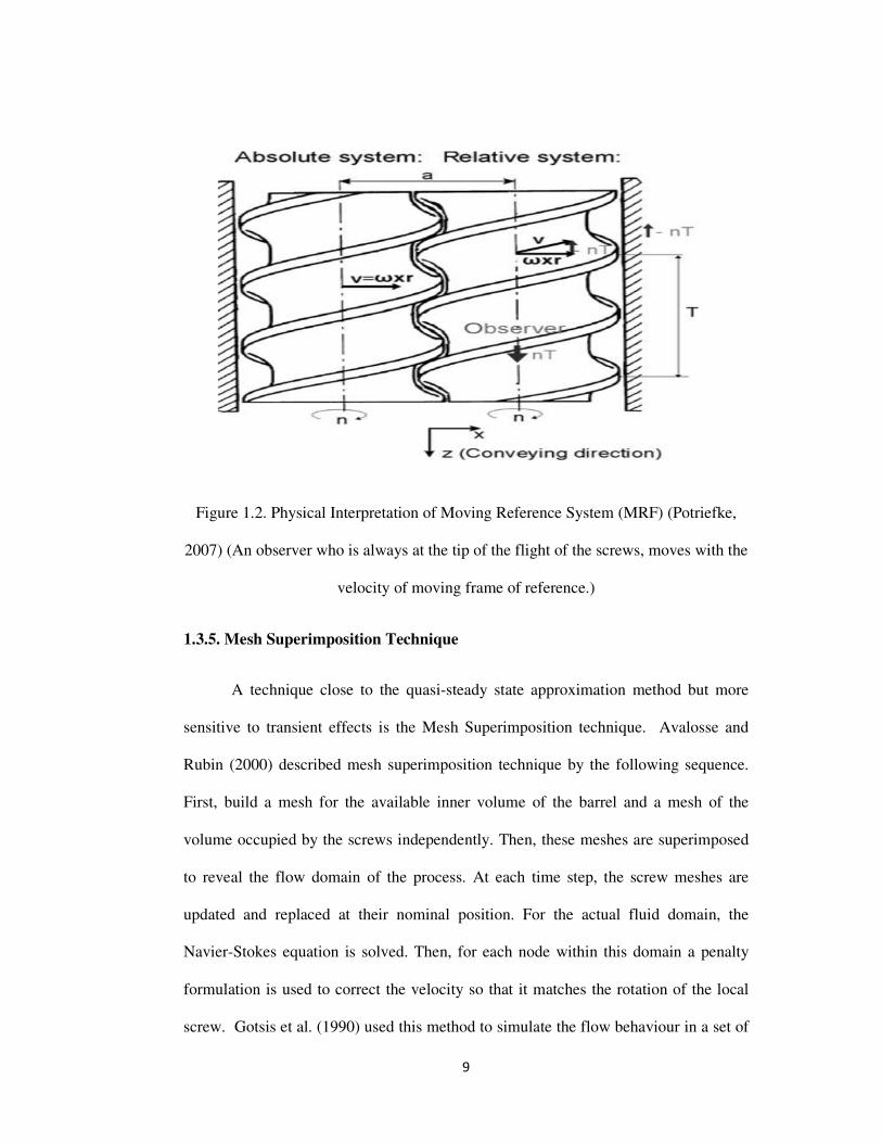
Figure 1.2. Physical Interpretation of Moving Reference System (MRF) (Potriefke,
2007) (An observer who is always at the tip of the flight of the screws, moves with the
velocity of moving frame of reference.) ........................................................................9
Figure 2.1. Schematic View of ICRTSE from MIKROSAN INC. I: Left Hand Screw
II: Right Hand Screw Detail A: Conveying Element Detail B: Mixing Element ........13
Figure 2.2. Screw Design Parameter ...........................................................................15
Figure 2.3. Viscosity Curve of Typical PVC (As Measured in a Rotational
Viscometer) ..................................................................................................................18
Figure 3.1. C-shaped Chamber (Fitzpatrick, 2009) .....................................................20
Figure 3.2. Overlapping Angle (Janssen, 1978) ..........................................................20
Figure 3.3. Geometrical Parameters for Simple Model of Theoretical Output ...........23
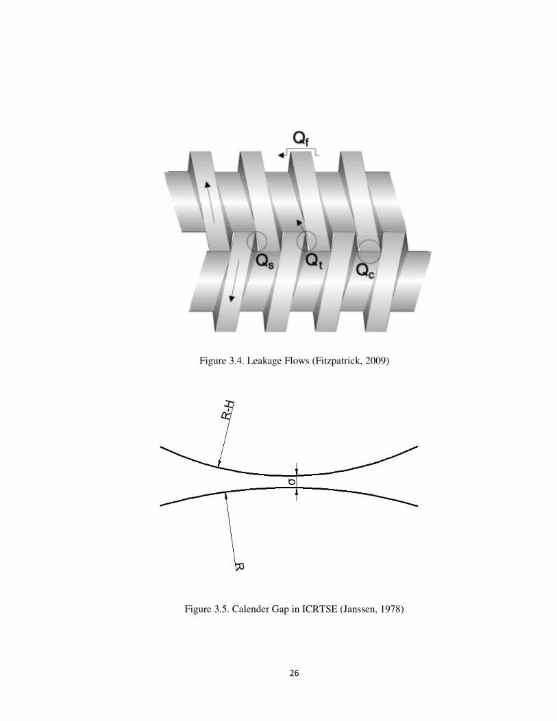
Figure 3.4. Leakage Flows (Fitzpatrick, 2009).............................................................26
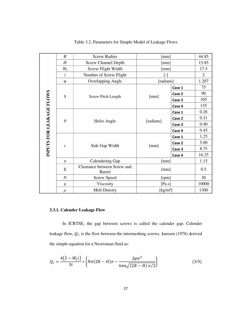
Figure 3.5. Calender Gap in ICRTSE (Janssen, 1978) ................................................26
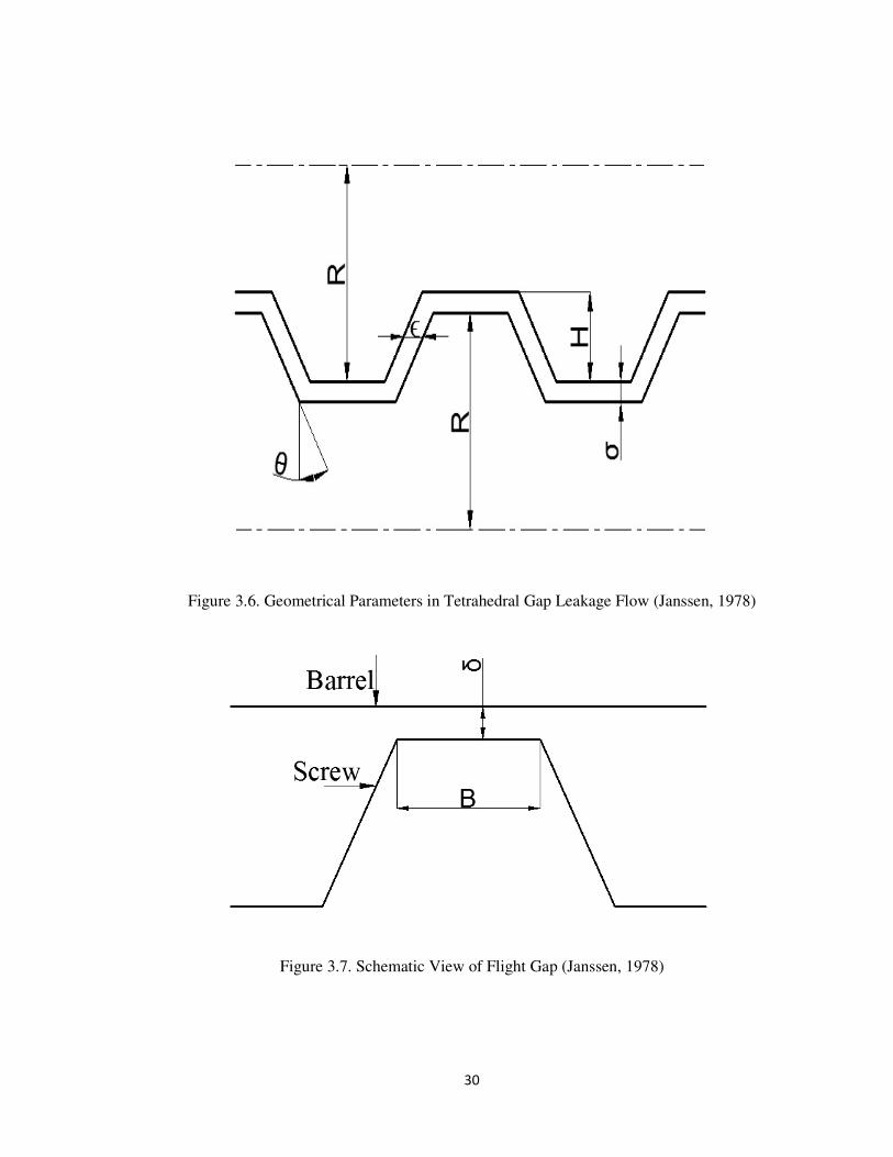
Figure 3.6. Geometrical Parameters in Tetrahedral Gap Leakage Flow (Janssen,
1978)………………………………………………………………………………….30
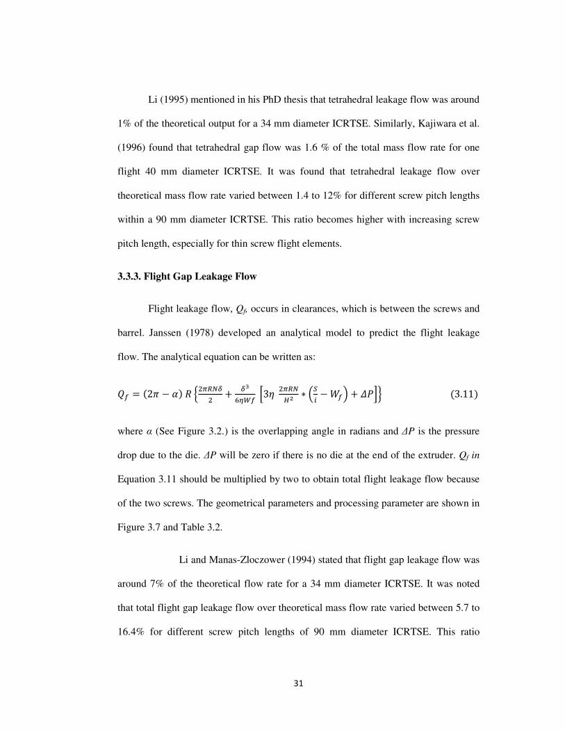
Figure 3.7. Schematic View of Flight Gap (Janssen, 1978) ........................................30
xii
Figure 3.8. Pumping Efficiency for Various Screw Pitch Lengths for Simple Model.37
Figure 3.9. Pumping Efficiency for Various Flight Width-to-channel Width Ratios..39
Figure 3.10. Pumping Efficiency for Various Screw Speeds for Simple Model .........40
Figure 4.1. Working Procedure of Current Study ........................................................44
Figure 4.2. Mesh Appearance of 105mm Screw Pitch Length ....................................51
Figure 4.3. Converging Residuals with Iteration Number for 105 mm Screw Pitch
Length ..........................................................................................................................52
Figure 5.1. Pressure Development between Two Co-rotating Cylinders ...................58
Figure 5.2. Pressure Development between Two Counter-rotating Cylinders ...........59
Figure 5.3. Pressure Distribution in a Journal Bearing ................................................62
Figure 6.1. Sequential Geometries Representing Complete Cycle ..............................65
Figure 6.2. Schematic View of the Location of Cross Sections and Boundaries ........66
Figure 6.3. Axial Velocity Distribution at Plane 1 α=90° for 105 mm Screw Pitch
Length ..........................................................................................................................72
Figure 6.4. Axial Velocity Distribution at Plane 2 α=90° for 105 mm Screw Pitch
Length ..........................................................................................................................73
Figure 6.5. Axial Velocity Distribution at Plane 3 α=90° for 105 mm Screw Pitch
Length ..........................................................................................................................74
xiii
Figure 6.6. Axial Velocity Distribution at Plane 4 α=90° for 105 mm Screw Pitch
Length ..........................................................................................................................75
Figure 6.7. The Effect of Screw Pitch Length on Pumping Efficiency .......................78
Figure 6.8. The Effect of Flight Width-to-channel Width Ratio on Pumping Efficiency
for Power Index 1, 0.7 and 0.3 .....................................................................................79
Figure 6.9. The Effect of Screw Speed on Pumping Efficiency for Power Index 1 ....80
Figure 6.10. The Effect of Screw Speed on Pumping Efficiency for Power Index
0.7.................................................................................................................................81
Figure 6.11. The Effect of Screw Speed on Pumping Efficiency for Power Index
0.3.................................................................................................................................82
Figure 6.12. Shear Stress Distribution at Plane 1 α=90° for 105 mm Screw Pitch
Length Power Index 0.7 ...............................................................................................86
Figure 6.13. Shear Stress Distribution at Plane 2 α=90° for 105 mm Screw Pitch
Length Power Index 0.7 ...............................................................................................87
Figure 6.14. Shear Stress Distribution at Plane 3 α=90° for 105 mm Screw Pitch
Length Power Index 0.7 ...............................................................................................88
Figure 6.15. Shear Stress Distribution at Plane 4 α=90° for 105 mm Screw Pitch
Length Power Index 0.7 ...............................................................................................89
Figure 6.16. The Volume Distribution of Shear Stress for 75 mm Screw Pitch Length
for Power Index 0.7 ....................................................................................................92
xiv
Figure 6.17. The Volume Distribution of Shear Stress for 105 mm Screw Pitch Length
for Power Index 0.7 .....................................................................................................93
Figure 6.18. The Volume Distribution of Shear Stress for 75 mm Screw Pitch Length
for Power Index 0.3 .....................................................................................................94
Figure 6.19. The Volume Distribution of Shear Stress for 105 mm Screw Pitch Length
for Power Index 0.3 .....................................................................................................95
Figure 6.20. The Average Shear Stress for Various Screw Speed and Screw Pitch
Length Power Index 0.7 ...............................................................................................96
Figure 6.21. The Average Shear Stress for Various Screw Speed and Screw Pitch
Length Power Index 0.3................................................................................................97
Figure 6.22. Mixing Parameter λ Distribution at Plane 1 α=90° for 105 mm Screw
Pitch Length Power Index 0.7 ....................................................................................101
Figure 6.23. Mixing Parameter λ Distribution at Plane 2 α=90° for 105 mm Screw
Pitch Length Power Index 0.7 ....................................................................................102
Figure 6.24. Mixing Parameter λ Distribution at Plane 3 α=90° for 105 mm Screw
Pitch Length Power Index 0.7 ....................................................................................103
Figure 6.25. Mixing Parameter λ Distribution at Plane 4 α=90° for 105 mm Screw
Pitch Length Power Index 0.7 ....................................................................................104
Figure 6.26. The Volume Distribution of Mixing Parameter λ for 75 mm Screw Pitch
Length for Power Index 0.7 .......................................................................................105
xv
Figure 6.27. The Volume Distribution of Mixing Parameter λ for 105 mm Screw Pitch
Length for Power Index 0.7 .......................................................................................106
Figure 6.28. The Volume Distribution of Mixing Parameter λ for 75 mm Screw Pitch
Length for Power Index 0.3 .......................................................................................107
Figure 6.29. The Volume Distribution of Mixing Parameter λ for 105 mm Screw Pitch
Length for Power Index 0.3 .......................................................................................108
Figure 6.30. The Average Mixing Parameter λ for Various Screw Speed and Screw
Pitch Length Power Index 0.7 ....................................................................................109
Figure 6.31. The Average Mixing Parameter λ for Various Screw Speed and Screw
Pitch Length Power Index 0.3 ....................................................................................110
Figure 7.1. Comparison of the Effect of Screw Pitch Length for Computer
Simulation and Simple Flow Model ..........................................................................113
Figure 7.2. Comparison of the Effect of the Flight Width-to-channel Width Ratio
for Computer Simulation and Simple Flow Model ...................................................114
Figure 7.3. Comparison of the Effect of Screw Speed for 75 mm and 90 mm Screw
Pitch Length for Computer Simulation and Simple Flow Model ..............................115
Figure 7.4. Comparison of the Effect of Screw Speed for 105 mm and 135 mm
Screw Pitch Length for Computer Simulation and Simple Flow Model ...................116
xvi
LIST OF TABLES
Table Page
Table 2.1 ICRTSE Geometrical Design Parameters ....................................................16
Table 3.1. Geometrical Parameters and Mass Flow Rate Results without Leakage
Flow .............................................................................................................................24
Table 3.2. Parameters for Simple Model of Leakage Flows........................................27
Table 3.3. Total Calender Leakage Flow for Various Screw Pitch Lengths ………...28
Table 3.4. Total Tetrahedral Gap Leakage Flow for Various Screw Pitch Lengths ....29
Table 3.5. Total Flight Gap Leakage Flow for Various Screw Pitch Lengths ………32
Table 3.6. Total Side Gap Leakage Flow for Various Screw Pitch Lengths ………...33
Table 3.7. Total Mass Flow Rate (Including Leakage Flows) for Various Screw Pitch
Lengths ………………………………………………………………………………34
Table 3.8. Total Mass Flow Rate (Including Leakage Flows) For Various Flight
Width-to-channel Width Ratios ……………………………………………………38
Table 3.9. Total Mass Flow Rate (Including Leakage Flows) for Various Screw
Speeds ………………………………………………………………………………..38
Table 4.1. Boundary Conditions for Velocity and Pressure ........................................48
Table 4.2. Different Number of Cells and Results for Various Cases .........................50
xvii
Table 5.1. Parameters Used in the Co- and Counter-rotating Cylinder Examples
Reported in Figures 5.1 and 5.2 ...................................................................................57
Table 6.1. Average Axial Velocities for Various α and for Screw Pitch Length for
Power Index 1 ..............................................................................................................69
Table 6.2. Average Axial Velocities for Various α and for Screw Pitch Length for
Power Index 0.7 ...........................................................................................................70
Table 6.3. Average Axial Velocities for Various α and for Screw Pitch Length for
Power Index 0.3 ...........................................................................................................71
Table 6.4. Average Shear Stress and Average Mixing Parameter for Various α and
Screw Pitch Length for Power Index 0.7 .....................................................................90
Table 6.5. Average Shear Stress and Average Mixing Parameter for Various α and
Screw Pitch Length for Power Index 0.3 .....................................................................91

xviii
LIST OF SYMBOLS
�� Velocity Vector
�� Rate of the Strain Tensor
�̿ Stress tensor
A Center Distance
Cp Specific Heat Capacity
eθ Unit Vector in θ direction
H Screw Channel Depth
i Number of Screw Flights
IID Second invariant of the Strain Rate Tensor
k Thermal Conductivity
n Power index
N Screw Speed
P Pressure
Qc Calender Leakage Flow
Qf Flight Gap Leakage Flow
Qs Side Gap Leakage Flow
Qt Tetrahedral Leakage Flow

xix
Qth Theoretical Flow Rate
Qtotal Total Flow Rate
R Screw Radius
r Radial Position of the Element
S Screw Pitch Length
Ux Velocity at x Direction
Uy Velocity at y Direction
Uz Velocity at z Direction
V Circular Path Velocity
V1 Volume of the One Barrel Half over One Pitch Length
V2 Volume of the Screw Root over One Pitch Length
V3 Volume of the Screw Flight
Vaxial Axial Velocity
Vc C-shaped chamber Volume
Wc Screw Channel width
Wf Screw Flight Width
α Overlapping Angle
δ Clearance Between Screw and Barrel
xx
∆p Local Pressure Difference Between Opposite C-shaped
Chamber
∆P Pressure Drop due to the Die
ϵ Side Gap Width
η Viscosity
η0 Viscosity at Zero Shear Rate
ηinf Viscosity at Infinity Shear Rate
θ Helix Angle
λ Dispersive Mixing Parameter
ρ Density
σ Calender Gap
ω Rate of the Vorticity Tensor
1
Chapter One
INTRODUCTION AND BACKGROUND
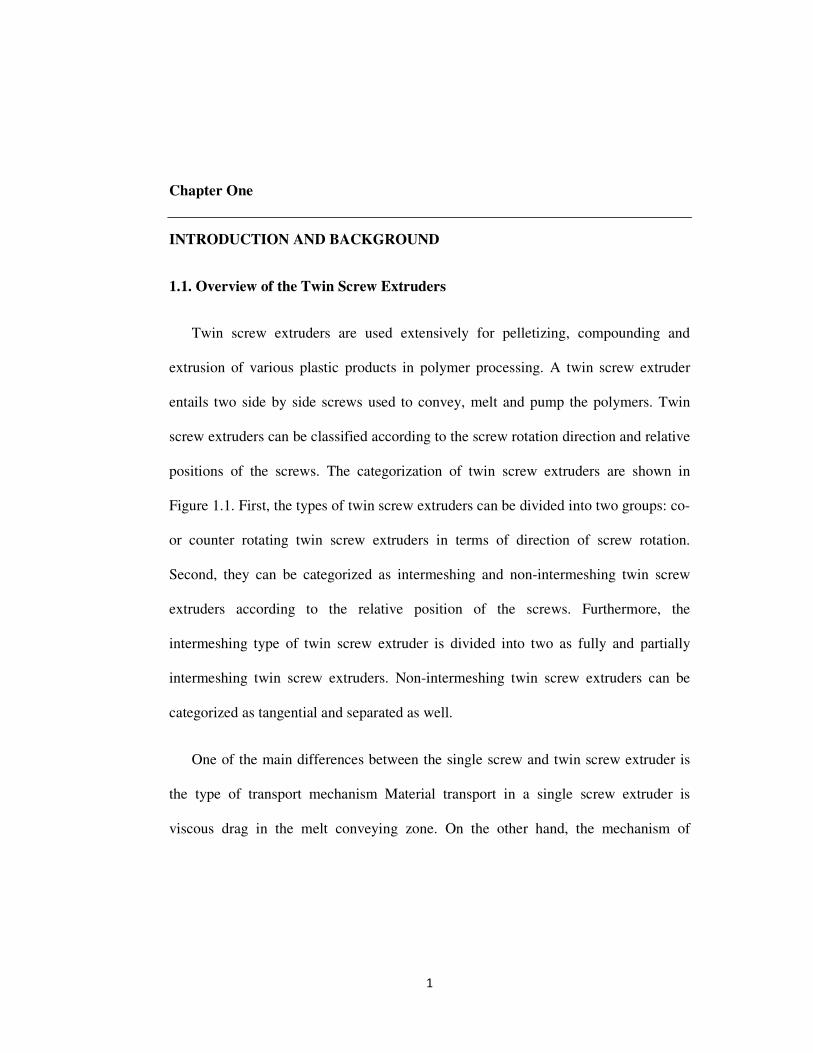
1.1. Overview of the Twin Screw Extruders
Twin screw extruders are used extensively for pelletizing, compounding and
extrusion of various plastic products in polymer processing. A twin screw extruder
entails two side by side screws used to convey, melt and pump the polymers. Twin
screw extruders can be classified according to the screw rotation direction and relative
positions of the screws. The categorization of twin screw extruders are shown in
Figure 1.1. First, the types of twin screw extruders can be divided into two groups: co-
or counter rotating twin screw extruders in terms of direction of screw rotation.
Second, they can be categorized as intermeshing and non-intermeshing twin screw
extruders according to the relative position of the screws. Furthermore, the
intermeshing type of twin screw extruder is divided into two as fully and partially
intermeshing twin screw extruders. Non-intermeshing twin screw extruders can be
categorized as tangential and separated as well.
One of the main differences between the single screw and twin screw extruder is
the type of transport mechanism Material transport in a single screw extruder is
viscous drag in the melt conveying zone. On the other hand, the mechanism of
2
Figure 1.1. Classification of Twin Screw Extruders (Cheremisinoff, 1987)
3
of transport in a twin screw extruder is positive displacement for its fluid transport.
Another main difference between single and twin screw extruders is the velocity
profile in the screw channel. The flow in twin screw is more complex than in the
single screw extruder. This complexity of the flow provides better mixing, heat
transfer and devolatilization.
Intermeshing counter-rotating twin screw extruders (ICRTSE) have better positive
displacement ability and are more suitable for shear sensitive materials compare to
other types of extruders. In addition, Eggen and Syre (2004) implied that having
counter-rotating screws are advantageous because they can be made shorter than co-
rotating machines. A shorter extruder gives an opportunity to save material and space.
It also simplifies the screw design because it is hard to prevent long screws from
flexing under load.
1.2. Intermeshing Counter-Rotating Twin Screw Extruders (ICRTSE)
Intermeshing counter-rotating twin screw extruders (ICRTSE) have their origins in
the 19th
century as positive displacement pumps. Positive displacement is defined in
this case as material transportation within a fully filled C-shaped chamber that only
allows bulk motion in one axial direction. ICRTSE are mainly utilized for pelletizing,
devolatilizing, polyvinyl chloride (PVC) pipes and profiles. ICRTSE have an
advantage by exhibiting a superior constant throughput compare to the other
extruders.
4
The ratio between the total throughput and theoretical throughput based on its C-
shaped chamber volume is called pumping efficiency. Pumping efficiency is the main
parameter for measuring performance of an ICRTSE. Doboczky (19652) suggested the
application of this factor by which the theoretical output must be multiplied in order to
arrive at experimental values. Doboczky (19652) stated that pumping efficiencies
varied for different screws from 0.17 to 0.64. Schenkel (1966) mentioned that the
efficiency of twin screw extruder lies between 34% and 41% for various extruders.
Menges and Klenk (1966) and Klenk (1971) improved the process, using
polyvinylchloride. It was reported that the experimental output versus the theoretical
prediction was in the range of 37 to 41% in their case.
Jiang (2008) investigated the pumping behaviour of ICRTSE for different ratios of
flight width-to-channel width, clearances between screw and barrel and helix angles in
his PhD thesis. It was found that thicker flighted elements had better pumping
efficiency. According to that author the pumping efficiency decreased with decreasing
power law index. It was also argued that a larger clearance between screw and barrel
caused lower pumping efficiency due to higher leakage flows. Finally, he mentioned
that there was little variation in pumping efficiency with changing helix angle.
Janssen et al. (1975) revealed that the throughput of ICRTSE increased linearly
with increasing screw speed for a 70mm screw diameter. Doboczky (19651, 1965
2)
stated that ICRTSE has about three times higher output capacity than the single screw
extruder for same size and the screw speed. Li and Manas-Zloczower (1994) stated
that pumping efficiency hardly ever changes with screw speed. Sakai et al. (1987)
made an experimental comparison between counter-rotation and co-rotation on the
5
twin screw extrusion performance. They mentioned that sharper residence time
distribution can be obtained when using the counter-rotating twin screw extruder for a
69 mm diameter twin screw extruder. Wolf et al. (1986) concluded that counter-
rotating twin screw extruders tend to behave like plug flow almost the entire extruder
length for a 90 mm diameter extruder. Shon et al. (1999) indicated that the lowest
mean residence time was obtained for the intermeshing twin screw extruder compare
to the buss kneader, continuous mixer, co-rotating twin screw extruder and counter-
rotating twin screw extruder. They showed that ICRTSE have near plug flow which
indicates a positive displacement mechanism. In present study, different geometries
of ICRTSE will be examined and effects on the pumping behaviour and dispersive
mixing will be discussed.
1.3. Modelling Twin Screw Extrusion
1.3.1. Analytical Modelling
Analytical models have been presented by various authors and these have been
reviewed by Janssen (1978) and White (1990). The analytical models are derived from
simply determination of positive displacement capacity on the basis of twin screw
geometry. The relevant models to this thesis and their limitations will be discussed in
Chapter 3.
1.3.2. Flow Analysis Network
A common simplified numerical method to simulate this twin screw extruder is
the Flow Analysis Network (FAN) method. The basic idea of the FAN method is to
divide the region into control volumes (CV) and carry out flux balances on each. One
6
of the first users of FAN method for modelling fluid flow in kneading elements of a
co-rotating twin screw extruder was Szydlowski et al. (1987). Sebastian and Rakos
(1990) compared FAN method and finite element method (FEM) for the mixing
section of the co-rotating twin screw extruder. Hong and White (1998) presented a
FAN method to understand a pumping characteristic of thick and thin flight elements
of counter-rotating twin screw extruder. However, this method is generally too
restrictive in both the geometries it can be applied to as well as the information
obtained, and hence other methods have been considered over time. What follows are
a series of techniques used to apply the finite element method (FEM) to numerically
simulate flow in a twin screw extruder – a system made complex due to its moving
screws. In FEM, the geometry of the fluid domain is divided into a number of cells.
Each cell is defined by nodal points and the neighbouring points connect to each
other. Flow patterns are described by the equations of continuity and momentum as
discretized partial differential equations in matrix form. The non-linear system of
equation is then solved to determine the velocity and pressure components.
1.3.3. Quasi Steady State Approximation
Twin screw extruders cannot reach a truly steady state condition because the
flow geometry being modelled is in constant motion rather than being fixed in space.
Lee and Castro (1989) mentioned that if the Reynolds number is very small, the time
dependent part of the continuum equation is negligible. The resulting quasi-steady
state solution is dependent only on instantaneous material properties and boundary
conditions. By this approximation, different relative positions of the screws into the
barrel are selected and simulated as a fixed, steady state system. Different meshes are
7
necessary for each relative position of the screw as it rotates and the results are
compiled together.
Yang and Manas-Zloczower (1992) used this method to simulate the dispersive
mixing behaviour of a Banbury mixer (which is a rotating screw system). Ishikawa et
al. (2000) applied this approach to simulate the pressure distribution of a 30 mm
diameter co-rotating twin screw extruder. Bravo (1998) explored this method to
understand the flow behaviour of a 45° stagger angle kneading element. Yao and
Manas-Zloczower (1997) followed the quasi-steady state approximation for the
mixing behaviour of the clearance mixer. Wang and Manas-Zloczower (1994) also
applied quasi-steady state for the mixing behaviour of cavity mixer. Li (1995)
simulated the intermeshing counter-rotating twin screw extruder and tangential
counter-rotating twin screw extruder in terms of mixing efficiency by using quasi-
steady state approximation in his PhD thesis. Recently, Sobhani et al. (2010) analyzed
the flow behaviour of co-rotating twin screw extruder with the same method.
There are two main disadvantages for quasi-steady state approximation. First, a
lot of meshing studies have to be done to accurately capture as many positions of
screws as possible. Second, this method does not work properly because the energy
equation is truly transient. Lee and Castro (1989) stated that neglecting the transient
term in the equation of motion was justified but not the transient term of the energy
equation.
1.3.4. Moving Reference Frame (MRF) Method
The alternative to the quasi-steady state approximation is to simulate the twin
screw extrusion by the moving reference frame (MRF) method. In the MRF
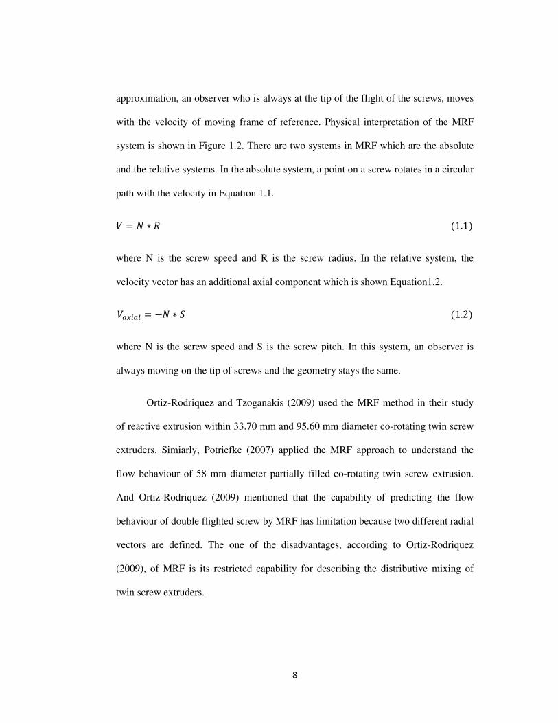
8
approximation, an observer who is always at the tip of the flight of the screws, moves
with the velocity of moving frame of reference. Physical interpretation of the MRF
system is shown in Figure 1.2. There are two systems in MRF which are the absolute
and the relative systems. In the absolute system, a point on a screw rotates in a circular
path with the velocity in Equation 1.1.
� = � ∗ (1.1)
where N is the screw speed and R is the screw radius. In the relative system, the
velocity vector has an additional axial component which is shown Equation1.2.
������ = −� ∗ �(1.2)
where N is the screw speed and S is the screw pitch. In this system, an observer is
always moving on the tip of screws and the geometry stays the same.
Ortiz-Rodriquez and Tzoganakis (2009) used the MRF method in their study
of reactive extrusion within 33.70 mm and 95.60 mm diameter co-rotating twin screw
extruders. Simiarly, Potriefke (2007) applied the MRF approach to understand the
flow behaviour of 58 mm diameter partially filled co-rotating twin screw extrusion.
And Ortiz-Rodriquez (2009) mentioned that the capability of predicting the flow
behaviour of double flighted screw by MRF has limitation because two different radial
vectors are defined. The one of the disadvantages, according to Ortiz-Rodriquez
(2009), of MRF is its restricted capability for describing the distributive mixing of
twin screw extruders.
9
Figure 1.2. Physical Interpretation of Moving Reference System (MRF) (Potriefke,
2007) (An observer who is always at the tip of the flight of the screws, moves with the
velocity of moving frame of reference.)
1.3.5. Mesh Superimposition Technique
A technique close to the quasi-steady state approximation method but more
sensitive to transient effects is the Mesh Superimposition technique. Avalosse and
Rubin (2000) described mesh superimposition technique by the following sequence.
First, build a mesh for the available inner volume of the barrel and a mesh of the
volume occupied by the screws independently. Then, these meshes are superimposed
to reveal the flow domain of the process. At each time step, the screw meshes are
updated and replaced at their nominal position. For the actual fluid domain, the
Navier-Stokes equation is solved. Then, for each node within this domain a penalty
formulation is used to correct the velocity so that it matches the rotation of the local
screw. Gotsis et al. (1990) used this method to simulate the flow behaviour in a set of
10
kneading discs within a co-rotating twin screw extruder. Alsteens et al. (2004)
evaluated this method to understand the mixing efficiency for said kneading elements
of a co-rotating twin screw extruder. Gupta et al. (2009) compared 30 mm diameter
co-rotating and counter-rotating twin screw extruders by this approach. The mesh
generation required for this method can very simple when a coarse pattern is used;
however, very coarse meshes can cause poor results for complex flow regions.
Considering the complexities inside a twin screw extrusion this is extremely
complicated and therefore was not chosen for the present thesis.
1.4. Objectives
There are three main objectives in this dissertation.
1. Carryout a comprehensive analysis of the flow mechanism in the conveying
element of counter-rotating twin screw extruder for various screw pitch
lengths, ratios of flight width-to-channel width and screw speeds to determine
the pumping efficiency. The objective is to understand the effects of
geometrical parameters and processing conditions in better detail than found in
previous literature. The quasi-steady state approximation has been used for
modelling the flow within an ICRTSE. A number of sequential geometries at
defined angles of position are selected to represent a complete cycle of rotation
in the time dependent moving boundary condition. This approach assumes that
the polymer melt flows at very low Reynolds number, such that it is reasonable
to neglect the transient term of motion equation. It is also assumed that the
flow channel of the extruder is fully filled with polymer melt.

11
2. Evaluate how a simple (analytical) model predicts flow rate for the extruder
relative to different operational/geometric parameters. Compare the computer
simulation and simple flow model in order to determine whether the simple
flow model is useful or not.
3. Characterize the dispersive mixing through the determination of shear stress
and mixing parameter λ. Investigate the effect of the geometrical parameters
and processing conditions on the dispersive mixing.
1.5. Outline
The thesis is divided into 7 chapters in addition to this introduction and
background. Chapter 2 is devoted to a description of geometrical parameters and
processing conditions that are used for the simple flow model and computer
simulations. Chapter 3 contains a simple flow model for various screw geometry and
processing conditions. Limitations of the simple model are discussed in Chapter 3 as
well. In Chapter 4, information is given setting up a computational fluid dynamics
simulation of the extruder with OpenFOAM® (CFD software). Chapter 5 is dedicated
to explaining negative pressures in rotating polymer processing machinery, obtained
by various researchers. Chapter 6 includes numerical results to understand the flow
behaviour and dispersive mixing for different screw geometries and processing
conditions. The simple flow model and computer simulations are compared in terms
of flow rate in Chapter 7. Conclusions and recommendations for future studies are
presented in Chapter 8.
12
Chapter Two
GEOMETRICAL PARAMETERS AND MATERIAL PROPERTIES
2.1. Introduction
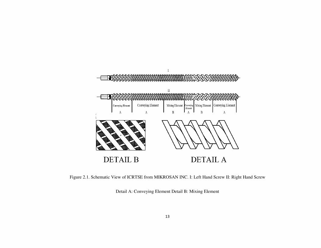
Before the simple model and computer simulation of intermeshing counter
rotating twin screw extruders (ICRTSE) are considered precisely, it is useful to
discuss screw geometries, material properties and processing conditions in detail.
ICRTSE include two screws which rotate in opposite directions. One screw has a left
hand flight while the other has a right hand flight as is shown in Figure 2.1.
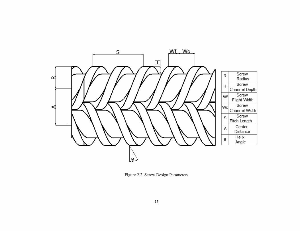
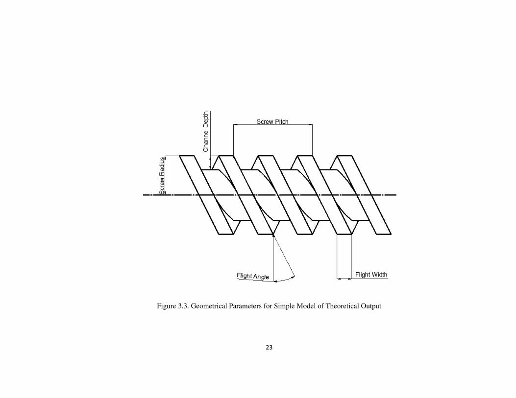
2.2. Geometrical Parameters
A schematic presentation of ICRTSE is shown in Figure 2.1. It is clear from
Figure 2.1 that the conveying element is the major type of screw element in ICRTSE.
The polymer material in the C-shaped chamber is pushed towards the die by positive
displacement in conveying elements. The polymer melt recirculates with the C-shaped
chamber, converging towards a narrow intermeshing region and then it diverges. The
geometrical parameters of ICRTSE that were used in this study are shown in Figure
2.2 and Table 2.1. Screw radius, R, channel depth, H, screw pitch length, S, flight
width, Wf, channel width, Wc, clearance between flight and barrel, δ, number of
flights, i, center distance, A, helix angle, θ, and flight width-to-channel width ratio are
the crucial design parameters for ICRTSE.
13
Figure 2.1. Schematic View of ICRTSE from MIKROSAN INC. I: Left Hand Screw II: Right Hand Screw
Detail A: Conveying Element Detail B: Mixing Element
14
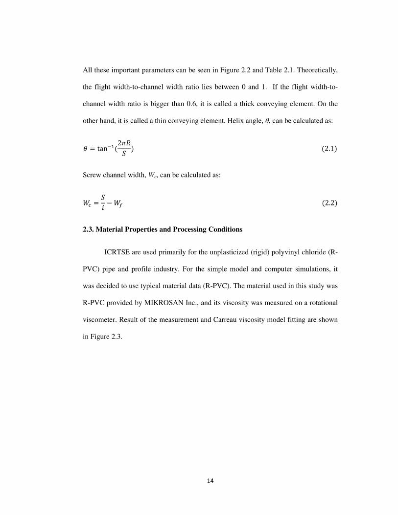
All these important parameters can be seen in Figure 2.2 and Table 2.1. Theoretically,
the flight width-to-channel width ratio lies between 0 and 1. If the flight width-to-
channel width ratio is bigger than 0.6, it is called a thick conveying element. On the
other hand, it is called a thin conveying element. Helix angle, θ, can be calculated as:
� = tan��(2�� )(2.1)
Screw channel width, Wc, can be calculated as:
�� = � − �!(2.2)
2.3. Material Properties and Processing Conditions
ICRTSE are used primarily for the unplasticized (rigid) polyvinyl chloride (R-
PVC) pipe and profile industry. For the simple model and computer simulations, it
was decided to use typical material data (R-PVC). The material used in this study was
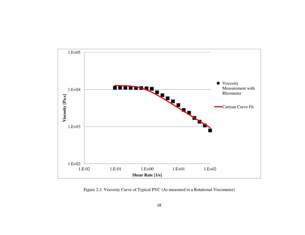
R-PVC provided by MIKROSAN Inc., and its viscosity was measured on a rotational
viscometer. Result of the measurement and Carreau viscosity model fitting are shown
in Figure 2.3.
15
Figure 2.2. Screw Design Parameters
16
Table 2.1 ICRTSE Geometrical Design Parameters
R Screw Radius [mm] 44.85
H Screw Channel Depth [mm] 15.85
Wf Screw Flight Width [mm] 17.5
i Number of Screw Flight [-] 2
A Center Distance [mm] 75
δ Clearance Between Screw and Barrel [mm] 0.5
S Screw Pitch Length [mm]
Case 1 75
Case 2 90
Case 3 105
Case 4 135
θ Helix Angle [°]
Case 1 14.90
Case 2 17.71
Case 3 20.44
Case 4 25.60
�!�� Flight Width / Channel Width Ratio [-]
Case 1 0.875
Case 2 0.636
Case 3 0.500
Case 4 0.350
17
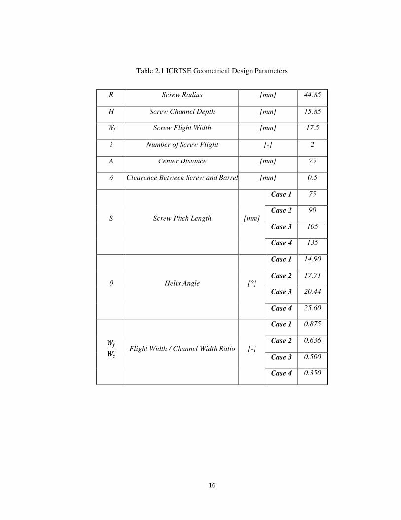
The Carreau viscosity model in Equation 2.3 was used for the shear rate
dependency of viscosity. In the Carreau model, η0 is the viscosity at zero shear rate,
ηinf is the viscosity at very high shear rates (important for solutions, but not for melts),
n is the power index, and λ is a relaxation time. Fitting of the data shown in Figure 2.3
gave η0 =12800 Pa.s (approximately), ηinf=10-12
Pa.s (assumed), n=0.47 and λ=1.4 s
(approximately). It was subsequently decided to use η0 =10000 Pa.s, λ=2 and n=1, 0.7,
0.3 to cover the usual range of polymer melts, likely to be processed in an ICRTSE.
Specific heat capacity, Cp, is assumed 1530 J/kg/°K and the melt density, ρ, is
assumed 1300 kg/m3.
"#!! = "�$! + &"' −"�$!((1 + ()��)*)$��* (2.3)
Figure 2.3 shows the viscosity curve of the typical R-PVC provided by
Mikrosan Inc. It has a zero shear viscosity, η0, of 10000 Pa.s and power index, n, of
0.47 at temperature 170°C. For the thesis study, the power index was not used but
rather altered. A power index of 1 was used for the Newtonian fluid simulations and
power indexes of 0.7 and 0.3 were used for Non-Newtonian fluid simulations.
Screw speed, N, is normally the main processing variable for controlling an
ICRTSE. Speeds of 30, 60 and 120 rpm were chosen to investigate. In this study, left
screw was rotated in the clockwise direction while right screw was rotated in the
counter-clockwise direction. Temperature dependency was never studied in this work.
18
Figure 2.3. Viscosity Curve of Typical PVC (As measured in a Rotational Viscometer)
1.E+02
1.E+03
1.E+04
1.E+05
1.E-02 1.E-01 1.E+00 1.E+01 1.E+02
Vis
cosi
ty [
Pa.s
]
Shear Rate [1/s]
Viscosity
Measurement with
Rheometer
Carreau Curve Fit
19
Chapter Three
A SIMPLE FLOW MODEL OF COUNTER-ROTATING TWIN SCREW
EXTRUDERS
3.1. Introduction
Intermeshing counter-rotating twin screw extruders (ICRTSE) are the closest
of this type of machine to exhibiting positive displacement while conveying process
material. Ideally, this means that all of the material in the system is pushed constantly
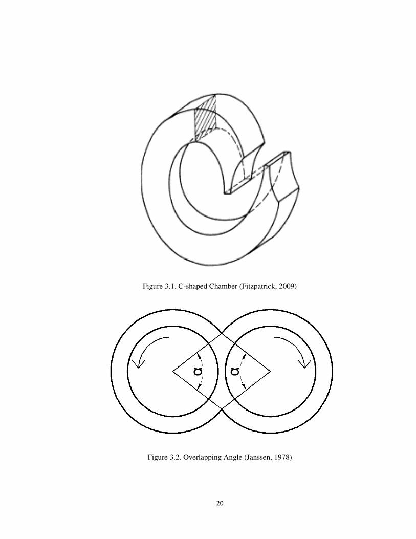
forwards no matter what the discharge pressure. In ICRTSE, the discrete volumes that
are filled by the polymers are called C-shaped chambers. The ICRTSE have been
modelled as a succession of C-shaped chambers by Janssen (1978). This simple flow
model is used to obtain throughput of ICRTSE. In this simple model, the C-shaped
chamber volume that is shown in Figure 3.1 combined with screw speed gives the
theoretical flow rate. By subtracting the total leakage flow from the theoretical flow
rate, the actual calculated output is obtained.
In this simple model, the chambers are assumed to be completely filled with
Newtonian fluid. The screws are also assumed to have uniform profiles in this zone
which means that the chamber and leakage gaps do not change as fluid moves along
the screws. Schenkel (1966), Doboczky (19651) analyzed the flow of a Newtonian
fluid within C-shaped chambers of an ICRTSE while neglecting leakage flows.
Janssen (1978) and White (1990) improved the accuracy of the simple flow
calculation by considering leakage flows.
20
Figure 3.1. C-shaped Chamber (Fitzpatrick, 2009)
Figure 3.2. Overlapping Angle (Janssen, 1978)
21
3.2. Simple Calculation of Output without Leakage Flow
Apparently, the first attempt to calculate the output of the intermeshing
counter-rotating multiple screw extruders for thermoplastics in the open literature was
by Schenkel (1963) who wrote:
,-. = /��� 0(3.1)
where Qth is the theoretical mass throughput, m is the number of screws, N is the
screw rotation speed, Vc is the C-shaped chamber volume per screw and ρ is the melt
density.
Doboczky (19651) modified Eq. (3.1) for twin screw machines as follows:
,-. = 2 ���0(3.2)
where i is the number of flights. Eq. (3.2) was also used by Janssen (1978) to develop
a more detailed analytical model for the ICRTSE. Janssen (1978) mentioned that the
C-shaped chamber volume can be calculated by subtracting the volume of a given
length of screw from the same length of the empty barrel.
The volume, V1, of one side of the inner barrel bore over one flight pitch length was
calculated as:
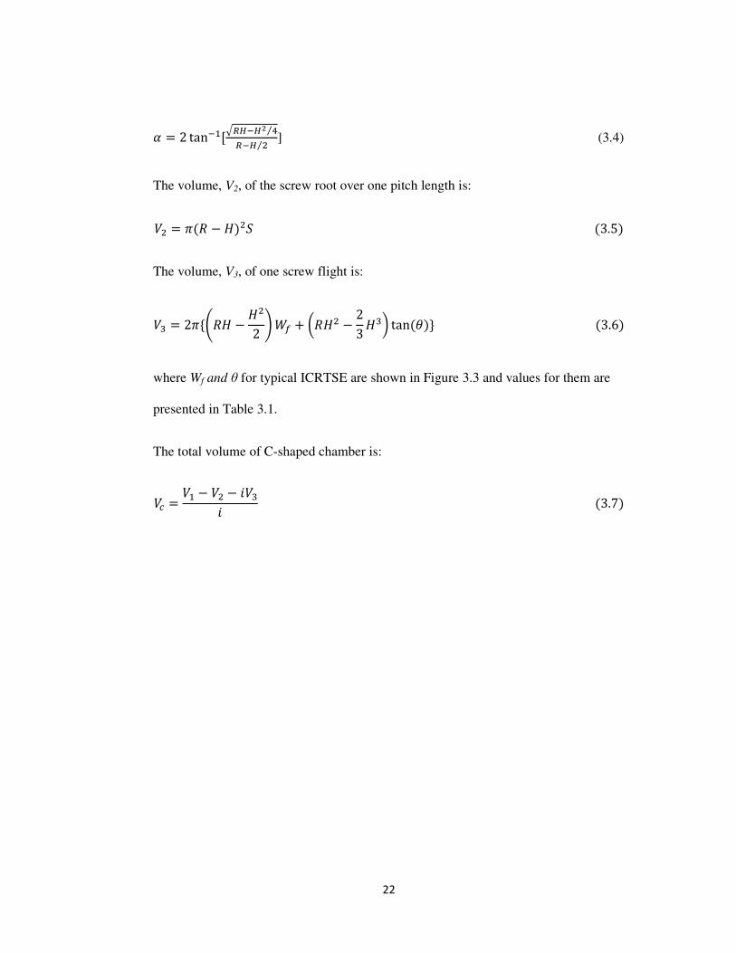
��= 12� − 3*4 * + 2 − 5*4 6(7 − 589 :S (3.3)
where the variables of R, H and S for typical ICRTSE are shown in Figure 3.3 and
values for these variables are presented in Table 3.1. α is defined as the overlapping
angle in radians (See Figure 3.2). It is given by the formula:
22
; = 2 tan��[=>5�58 9⁄>�5 *⁄ ] (3.4)
The volume, V2, of the screw root over one pitch length is:
�* = �( − 7)*�(3.5)
The volume, V3, of one screw flight is:
�A = 2�{C7 − 7*2 D �! + E7* − 23 7AF tan(�)}(3.6)
where Wf and θ for typical ICRTSE are shown in Figure 3.3 and values for them are
presented in Table 3.1.
The total volume of C-shaped chamber is:
�� = �� − �* − �A (3.7)
23
Figure 3.3. Geometrical Parameters for Simple Model of Theoretical Output
24
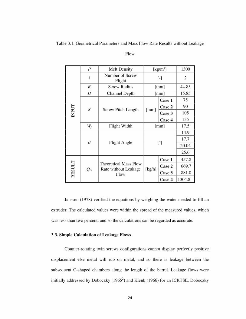
Table 3.1. Geometrical Parameters and Mass Flow Rate Results without Leakage
Flow
INP
UT
Ρ Melt Density [kg/m³] 1300
i Number of Screw
Flight [-] 2
R Screw Radius [mm] 44.85
H Channel Depth [mm] 15.85
S Screw Pitch Length [mm]
Case 1 75
Case 2 90
Case 3 105
Case 4 135
Wf Flight Width [mm] 17.5
θ Flight Angle [°]
14.9
17.7
20.04
25.6
RE
SU
LT
Qth
Theoretical Mass Flow
Rate without Leakage
Flow
[kg/h]
Case 1 457.8
Case 2 669.7
Case 3 881.0
Case 4 1304.8
Janssen (1978) verified the equations by weighing the water needed to fill an
extruder. The calculated values were within the spread of the measured values, which
was less than two percent, and so the calculations can be regarded as accurate.
3.3. Simple Calculation of Leakage Flows
Counter-rotating twin screws configurations cannot display perfectly positive
displacement else metal will rub on metal, and so there is leakage between the
subsequent C-shaped chambers along the length of the barrel. Leakage flows were
initially addressed by Doboczky (19652) and Klenk (1966) for an ICRTSE. Doboczky
25
(19652) indicated that leakage flows occur in the four areas that are shown in Figure
3.4. The first of these leakage flows is the calender leakage flow, Qc. This is the
leakage between the screw flight and the screw root. The second type of leakage is
tetrahedral gap leakage flow, Qt, which is the back flow through the tetrahedral gap
between the flanks of screws. The third type of leakage flow is the flight gap leakage
which is defined as flow of material over the flights of screws, Qf. Flight gap leakage
flow occurs between the barrel and screw flight, away from the intermeshing region.
The fourth is the side gap leakage flow, Qs, which is flow between the flanks of two
screws flight. Two pressure sources were identified by Janssen (1978) for this simple
model. The first source is the pressure which is developed at the die. This source from
the die is assumed zero in this simple model due to the isolating effect of each
chamber from the next. Janssen (1978) explained the second source of pressure as
moving wall of the extruder and the flow which occurs within the chamber itself.
Janssen (1978) wrote the second source of pressure as:
∆K = 6" 2��7* E� − �!F(3.8)
where ∆p is the local pressure difference between opposite C-shaped chambers, R is
the screw radius, S is the screw pitch length, i is the number of screw flight, Wf is the
flight width and N is the screw speed. All the geometrical parameters for a typical
ICRTSE are given in Table 3.2.
26
Figure 3.4. Leakage Flows (Fitzpatrick, 2009)
Figure 3.5. Calender Gap in ICRTSE (Janssen, 1978)
27
Table 3.2. Parameters for Simple Model of Leakage Flows
INP
UT
S F
OR
LE
AK
AG
E F
LO
WS
R Screw Radius [mm] 44.85
H Screw Channel Depth [mm] 15.85
Wf Screw Flight Width [mm] 17.5
i Number of Screw Flight [-] 2
α Overlapping Angle [radians] 1.207
S Screw Pitch Length [mm]
Case 1 75
Case 2 90
Case 3 105
Case 4 135
θ Helix Angle [radians]
Case 1 0.26
Case 2 0.31
Case 3 0.40
Case 4 0.45
ϵ Side Gap Width [mm]
Case 1 1.25
Case 2 5.00
Case 3 8.75
Case 4 16.25
σ Calendering Gap [mm] 1.15
δ Clearance between Screw and
Barrel [mm] 0.5
N Screw Speed [rpm] 30
η Viscosity [Pa.s] 10000
ρ Melt Density [kg/m³] 1300
3.3.1. Calender Leakage Flow
In ICRTSE, the gap between screws is called the calender gap. Calender
leakage flow, Qc, is the flow between the intermeshing screws. Janssen (1978) derived
the simple equation for a Newtonian fluid as:
,� = 4&� − �! (3 ∗ 1��(2 − 7)N − ∆KNA6�"=(2 − 7) N 2⁄ :(3.9)
28
Since there are four calender gaps in ICRTSE for the two flights per screw pitch, the
Qc in Equation 3.9 should be multiplied by four to obtain the total calender leakage
flow per C-shaped chamber. The calculated total calendar leakage flows for the
conditions examined in this work are shown in Table 3.3.
Speur et al. (1987) determined that the calender leakage flow rate over
theoretical flow rate changed between 10 to 44% for various geometries. Li (1995)
found that calender leakage flow was around 11% of the theoretical output for a 34
mm diameter ICRTSE while Kajiwara et al. (1996) found it to be 5% of the total flow
rate for a smaller one flight 40 mm diameter ICRTSE. As shown in Table 3.3, the
total calender leakage flow over theoretical mass flow rate varies between 12.5 to
14.4% for different screw pitch lengths of 90 mm diameter ICRTSE. This ratio does
not change sufficiently with increasing screw pitch length; however, the amount of
total calender leakage flow increases with increasing screw pitch length.
Table 3.3. Calender Leakage Flow for Various Screw Pitch Lengths
S Screw Pitch Length [mm]
Case 1 75
Case 2 90
Case 3 105
Case 4 135
Qc Total Calender Leakage
Flow [kg/h]
Case 1 66.14
Case 2 90.7
Case 3 115.2
Case 4 163.8
Qc /Qth
Total Calender
Leakage Flow /
Theoretical Mass
Flow Rate
[-]
Case 1 0.144
Case 2 0.135
Case 3 0.130
Case 4 0.125
29
3.3.2. Tetrahedral Gap Leakage Flow
In ICRTSE, another gap exists between screw flight walls. As can be seen in
Figure 3.4, the gap is approximately tetrahedral, Qt. Janssen (1978) developed a
simple model for tetrahedral gap leakage flow by using dimensional analysis and
regression analysis of the measurements. That simple model can be written as:
,- = ∆K ∗ A" ∗ 0.0054 ∗ E7F�.Q ∗ C� + 2 ∗ ER + N ∗ STU�7 F*D(3.10)
where ϵ is the width of the side gap and σ is the calender gap. There is only one
tetrahedral gap per C-shaped chamber. All the parameters used in the calculation can
be seen in Figure 3.6 with representative values given in Table 3.2.
Table 3.4. Tetrahedral Gap Leakage Flow for Various Screw Pitch Lengths
S Screw Pitch Length [mm]
Case 1 75
Case 2 90
Case 3 105
Case 4 135
Qt Tetrahedral Gap
Leakage Flow [kg/h]
Case 1 6.59
Case 2 17.56
Case 3 42.40
Case 4 158.84
Qt /Qth
Total Tetrahedral Gap
Leakage Flow /
Theoretical Mass
Flow Rate
[-]
Case 1 0.014
Case 2 0.026
Case 3 0.048
Case 4 0.12
30
Figure 3.6. Geometrical Parameters in Tetrahedral Gap Leakage Flow (Janssen, 1978)
Figure 3.7. Schematic View of Flight Gap (Janssen, 1978)
31
Li (1995) mentioned in his PhD thesis that tetrahedral leakage flow was around
1% of the theoretical output for a 34 mm diameter ICRTSE. Similarly, Kajiwara et al.
(1996) found that tetrahedral gap flow was 1.6 % of the total mass flow rate for one
flight 40 mm diameter ICRTSE. It was found that tetrahedral leakage flow over
theoretical mass flow rate varied between 1.4 to 12% for different screw pitch lengths
within a 90 mm diameter ICRTSE. This ratio becomes higher with increasing screw
pitch length, especially for thin screw flight elements.
3.3.3. Flight Gap Leakage Flow
Flight leakage flow, Qf, occurs in clearances, which is between the screws and
barrel. Janssen (1978) developed an analytical model to predict the flight leakage
flow. The analytical equation can be written as:
,! = (2� − ;) V*W>XY* + YZ[\]! ^3" *W>X58 ∗ 2_� − �!4 + `abc(3.11)
where α (See Figure 3.2.) is the overlapping angle in radians and ∆P is the pressure
drop due to the die. ∆P will be zero if there is no die at the end of the extruder. Qf in
Equation 3.11 should be multiplied by two to obtain total flight leakage flow because
of the two screws. The geometrical parameters and processing parameter are shown in
Figure 3.7 and Table 3.2.
Li and Manas-Zloczower (1994) stated that flight gap leakage flow was
around 7% of the theoretical flow rate for a 34 mm diameter ICRTSE. It was noted
that total flight gap leakage flow over theoretical mass flow rate varied between 5.7 to
16.4% for different screw pitch lengths of 90 mm diameter ICRTSE. This ratio

32
increased with decreasing screw pitch length especially for thick screw flight
elements.
Table 3.5. Total Flight Gap Leakage Flow for Various Screw Pitch Lengths
S Screw Pitch Length [mm]
Case 1 75
Case 2 90
Case 3 105
Case 4 135
Qf Total Flight Gap Leakage Flow [kg/h]
Case 1 75.14
Case 2 75.18
Case 3 75.24
Case 4 75.27
Qf /Qth
Total Flight Gap
Leakage Flow / Theoretical Mass
Flow Rate
[-]
Case 1 0.164
Case 2 0.112
Case 3 0.085
Case 4 0.057
3.3.4. Side Gap Leakage Flow
The last type of gap yielding leakage is the side gap which is between the
flanks of the flights in ICRTSE. Janssen (1978) developed a simple analytical model
for this side gap leakage flow, Qs. The calculation can be made as:
,d = ��(2 − 7)(7 − N)(R + N tan(�))(3.12) The geometrical parameters and processing parameters are shown in Figure 3.6 with
values given in Table 3.2. Since there are four side gaps per C-shaped chamber, the Qs
in Equation 3.12 should be multiplied by four to obtain total side gap leakage flow.
33
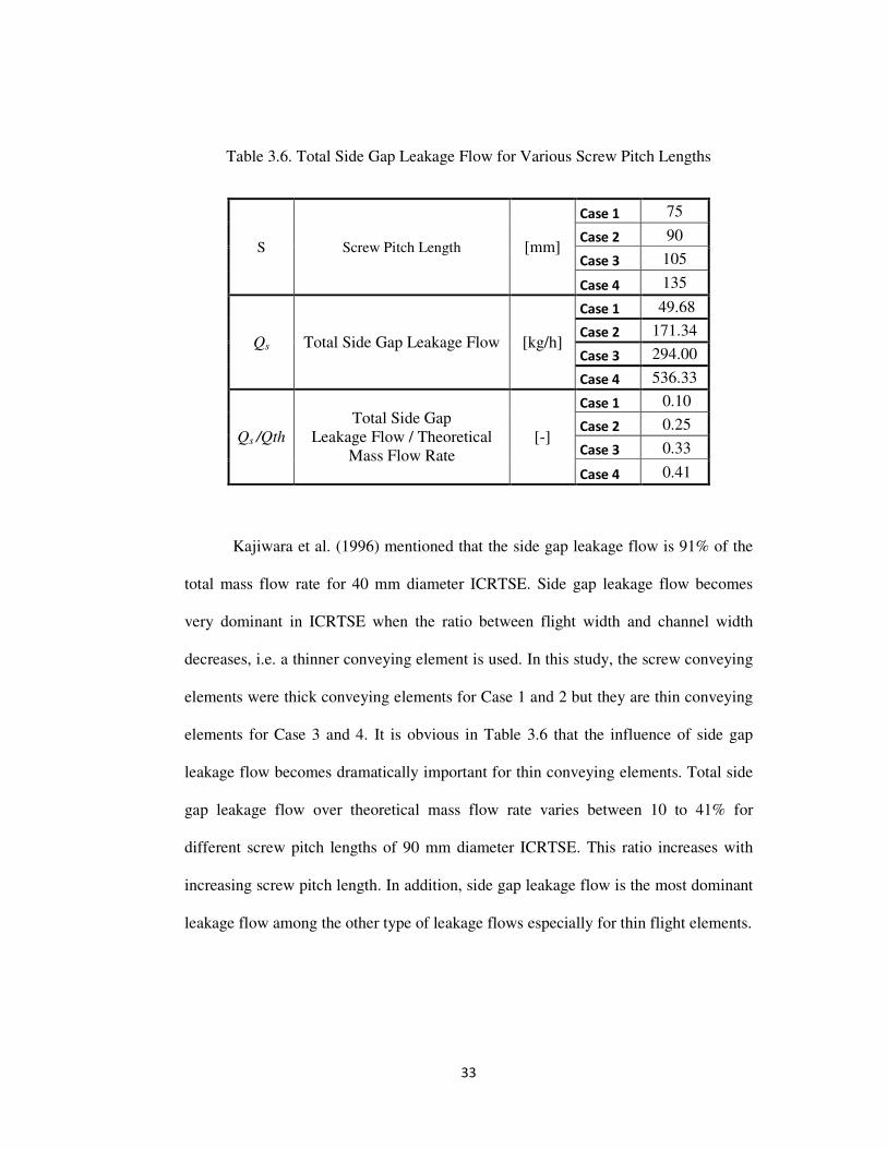
Table 3.6. Total Side Gap Leakage Flow for Various Screw Pitch Lengths
S Screw Pitch Length [mm]
Case 1 75
Case 2 90
Case 3 105
Case 4 135
Qs Total Side Gap Leakage Flow [kg/h]
Case 1 49.68
Case 2 171.34
Case 3 294.00
Case 4 536.33
Qs /Qth
Total Side Gap
Leakage Flow / Theoretical
Mass Flow Rate
[-]
Case 1 0.10
Case 2 0.25
Case 3 0.33
Case 4 0.41
Kajiwara et al. (1996) mentioned that the side gap leakage flow is 91% of the
total mass flow rate for 40 mm diameter ICRTSE. Side gap leakage flow becomes
very dominant in ICRTSE when the ratio between flight width and channel width
decreases, i.e. a thinner conveying element is used. In this study, the screw conveying
elements were thick conveying elements for Case 1 and 2 but they are thin conveying
elements for Case 3 and 4. It is obvious in Table 3.6 that the influence of side gap
leakage flow becomes dramatically important for thin conveying elements. Total side
gap leakage flow over theoretical mass flow rate varies between 10 to 41% for
different screw pitch lengths of 90 mm diameter ICRTSE. This ratio increases with
increasing screw pitch length. In addition, side gap leakage flow is the most dominant
leakage flow among the other type of leakage flows especially for thin flight elements.
34
3.4. Simple Model of Total Output
Ideally, the total output of the ICRTSE for double flighted screws (i.e. two
screw flights per turn) follows a mass balance equation:
,-e-�� = ,-. − ,- − 2,! − 4,� − 4,d(3.13)
where Qtotal is the total mass throughput, Qt is the tetrahedral leakage flow, Qf is the
flight gap leakage flow, Qc is the calender leakage flow and Qs is the side gap leakage
flows. Total mass throughputs are shown in Table 3.7 for various screw pitch length.
Table 3.7. Total Mass Flow Rate (Including Leakage Flows) for Various Screw Pitch
Lengths
S Screw Pitch Length [mm]
Case 1 75
Case 2 90
Case 3 105
Case 4 135
Qtotal Total Mass Flow Rate
(Including Leakage Flows) [kg/h]
Case 1 259.32
Case 2 313.63
Case 3 353.82
Case 4 367.79
Qtotal/Qth
Total Mass Flow Rate
(Including Leakage
Flows)/Theoretical Mass Flow
Rate
[-]
Case 1 0.566
Case 2 0.468
Case 3 0.401
Case 4 0.281
It can be seen in Table 3.7 that total mass flow rate increase gradually by
increasing screw pitch length. The pumping efficiency of an ICRTSE is a critical
parameter for measuring its performance. The pumping efficiency is defined as the
ratio between total mass flow rate and the theoretical throughput. Total mass flow
35
over theoretical mass flow rate (pumping efficiency) varies between 28 to 56% for
different screw pitch lengths of 90 mm diameter ICRTSE in Figure 3.8. In addition,
the results for pumping efficiency are plotted decreasing with increasing screw pitch
length. This is because the tetrahedral and side gaps become larger as the screw pitch
length increases. Hence, those gaps cause more leakage flow. The pumping
efficiencies of simple model of ICRTSE are same range as Doboczky (19652),
Schenkel (1966), Klenk (1971) and Li and Manas-Zloczower (1994).
The ratio of flight width and channel width is the one of the important
geometrical parameters. In this work flight width-to-channel width ratios of 0.875,
0.636, 0.500 and 0.350 were used. Table 3.8 indicated that the total mass flow rate
increases slightly by decreasing the ratio of the flight width to the channel width. In
addition Figure 3.9 shows that the pumping efficiency goes up with increasing flight
width-to-channel width ratio. Thicker flight elements have a better pumping behaviour
than the thin flight elements.
Another parameter that was investigated in this study is screw speed. Screw
speeds of 30, 60, and 120 rpm were selected in order to understand their influence on
the pumping behaviour of an ICRTSE. Total mass flow rates, Qtotal, are shown in
Table 3.9 for various screw speeds. It can be seen in Table 3.9 and Figure 3.10 that the
total mass throughput, Qtotal, increased linearly with screw speed; however, the
pumping efficiency did not change with screw speed. It is because while the total
throughput, Qtotal, increased linearly with screw speed, the theoretical output, Qth,
increased in the same manner.

36
Li and Manas-Zloczower (1994) showed that the ratio between leakage flow
and total leakage flow hardly ever changes with screw speed for a 34 mm diameter
ICRTSE.
37
Figure 3.8. Pumping Efficiency for Various Screw Pitch Lengths for Simple Model
0
0.1
0.2
0.3
0.4
0.5
0.6
75 90 105 120 135
Pu
mp
ing
Eff
icie
ncy
[-]
Screw Pitch Length [mm]
Simple Model
38
Table 3.8. Total Mass Flow Rate (Including Leakage Flows) For Various Flight
Width-to-channel Width Ratios
Wf/Wc Flight Width/Channel Width [-]
Case 1 0.875
Case 2 0.636
Case 3 0.500
Case 4 0.350
Qtotal Total Mass Flow Rate
(Including Leakage Flows) [kg/h]
Case 1 259.32
Case 2 313.63
Case 3 353.82
Case 4 367.79
Table 3.9. Total Mass Flow Rate (Including Leakage Flows) for Various Screw
Speeds
Screw Speed Screw Pitch
Length
Total Mass Flow Rate
(Including Leakage Flows)
N S Qtotal
[rpm] [mm] [kg/h]
30
75
259.32
60 519.53
120 1039.08
30
90
313.63
60 628.93
120 1257.86
30
105
353.82
60 710.31
120 1420.63
30
135
367.79
60 740.96
120 1481.93
39
Figure 3.9. Pumping Efficiency for Various Flight Width-to-channel Width Ratios
0
0.1
0.2
0.3
0.4
0.5
0.6
0.20 0.40 0.60 0.80 1.00
Pu
mp
ing
Eff
icie
ncy
[-]
Flight Widt/Channel Width
Simple Model
40
Figure 3.10. Pumping Efficiency for Various Screw Speeds for Simple Model
0
0.1
0.2
0.3
0.4
0.5
0.6
0 30 60 90 120
Pu
mp
ing
Eff
icie
ncy
[-]
Screw Speed [rpm]
75 mm Screw
Pitch
90 mm Screw
Pitch
105 mm Screw
Pitch
135 mm Screw
Pitch
41
3.5. Limitations of the Simple Model
The simple model provides a reasonable result about the pumping behaviour of
ICRTSE, yet it has some limitations. First and foremost, the simple model is valid for
Newtonian fluids but the materials used in the polymer processing industry are non-
Newtonian. Pressure due to the die in leakage flows is not taken into account and
these negative flows are also affected by non-Newtonian behavior. Then, the simple
model of ICRTSE can only predict throughput but the shear stress distribution,
velocity distribution, etc., are important as well to better understanding the ICRTSE.
Last but not least, the simple model of ICRTSE is only valid for parallel ICRTSE but
conical ICRTSE is also very common in polymer processing industry; however, this
issue has no relevance to the present thesis. Finally, the simple model assumes that
there is no die at the end of extruder, which neglects pressure effects and the screw
channels are fully filled with molten polymer, which is perhaps the least erroneous of
all stated assumptions.
To conclude, the simple model for ICRTSE can be an excellent starting point
but numerical models are necessary to better understand flow behaviour and ICRTSE
performance.
42
Chapter Four
COMPUTER SIMULATION USING OPENFOAM®
4.1. Introduction
Computational fluid dynamics (CFD) use numerical schemes to solve and
analyze problems related to fluid flow in complex environments. Availability of high
speed computers has made solving huge numbers of equations simultaneously quite
routine.
Basically, using CFD follows three steps. Pre-processing is the first step that
includes mesh generation, boundary condition determination as well as designation of
fluid properties. Secondly, numerical equations are solved based on the properties
that are determined in pre-processing step. Finally, the results are visualized in the
post-processing step.
Open Field Operation and Manipulation (OpenFOAM®) is the open source
CFD package developed by Open CFD Ltd. It was released in 2004 under the General
Public Licence. Fundamentally, the OpenFOAM® package use libraries to create
executable files, defined as applications, to solve the numerical equations. Since two
types of applications are valid in OpenFOAM®, solvers are used to solve numerical
equations while utilities are used to manipulate the data.
43
4.2. Numerical Analysis
The various screw geometries to be meshed and solved were provided by
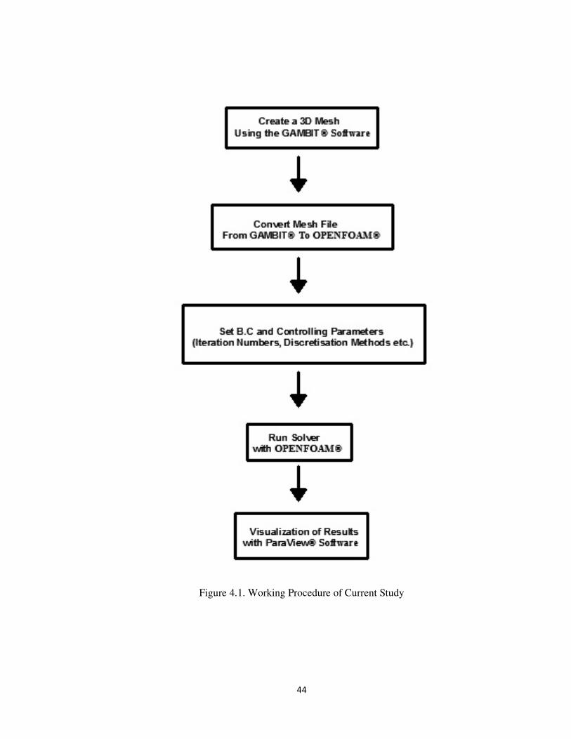
MIKROSAN Inc. In this study, the procedure was followed is shown in Figure 4.1.
GAMBIT® is geometry and mesh generation software. Firstly, 3D meshes were
created for the various screw pitch lengths in GAMBIT®. Secondly, the created
GAMBIT® mesh files were converted to OpenFOAM® mesh file style. Furthermore,
boundary conditions (mentioned in Sec. 4.3) and controlling parameters (iteration
numbers, discretisation methods etc.) were set. Then, the solver was executed on
Canada`s supercomputer network, Sharcnet, using four processors. The CPU time
required to perform the flow simulations varied between 80000 and 100000 s,
depending on the flow conditions and different type of geometries of ICRTSE
employed. Lastly, the results were examined and presented by using open source
scientific visualization software, ParaView®.
4.2.1. Solvers
OpenFOAM® includes around 80 standard solvers for different kind of
problems. In addition, OpenFOAM® has the ability to develop a new solver or
modify an existing solver for customized cases. In this study, the solver was chosen
for steady, incompressible fluid flow under laminar conditions. The chosen solver
used the SIMPLE algorithm, which stands for Semi Implicit Methods Pressure Linked
Equations, to solve mass and momentum as shown in Equations 4.1 and 4.2. This
algorithm minimizes simulation instabilities that otherwise arise when solving
velocity and pressure simultaneously.
44
Figure 4.1. Working Procedure of Current Study
45
Conservation of mass for an incompressible fluid and conservation of momentum for
laminar creepy flow (Reynolds number much smaller than 1) are shown in Equations
4.1 and 4.2 respectively. Shear thinning viscosity model and strain rate tensor are
given in Equations 4.3 and 4.4.
∇. �� = 0(4.1) −∇a + ∇. τh = 0(4.2)
τh = η(IIk)2lm(4.3)
ln = 12 (∇�� + ∇��o) = 12 Cp��pqr + p�rpq�D(4.4)
where �� is the velocity vector, P is the pressure, �̿ is the stress tensor, IID is the second
(scalar) invariant of the strain rate tensor, i and j equals 1, 2, 3. Juretic (2004)
explained the SIMPLE algorithm as follows: First of all, the initial guess is
determined. Secondly, the velocity field is calculated from the momentum equation by
the using initial guess. The momentum equation is solved under relaxation in order to
decrease non-linearity effect. Since the resulting velocity does not satisfy the
momentum equation, the pressure equation is solved by using the predicted velocity to
obtain new pressure field. Finally, it is repeated until the solution converges. The
chosen solver was modified to compute shear stress, shear rate and vorticity tensor.
4.2.2. Utilities
Utilities in OpenFOAM® provide data transformation and manipulation. More
than two hundreds utilities are present for different purposes. On top of that,
OpenFOAM® has the ability to develop new utilities or to modify current utilities for
46
customized cases. In this study, a lot of utilities were used but the most frequent ones
will be explained.
The first common utility is to convert to a GAMBIT® mesh file to an
OpenFOAM® mesh file, including multiple region and boundaries. The second
useful utility is to check mesh quality. This utility provides mesh statics, topology
checking, geometry checking and the sufficiency of a mesh for a simulation run. In
this study, the results showed that the mesh quality, which was obtained by this utility,
was always good. Another useful utility was used to calculate mass flow through
selected face sets or boundary patches for incompressible flow. This utility should be
used after the numerical solution converged. Last but not least, a utility was used to
extract data such as final residuals, iteration number etc., for plotting the profile of
data over time. Figure 4.3, for example, was created by using this utility.
4.3. Boundary Conditions
Four different boundary conditions are specified for velocity and pressure. The
boundary conditions that were used in this study are listed in Table 4.1.
Firstly, the standard no-slip boundary condition was used since slip concerns with
PVC are unlike to be important far from the die. This meant that the barrel velocity
boundary condition was:
s� = st = su = 0(4.5)

47
svvw = �. xyzvvvvw(4.6)
Secondly, boundary condition for rotating screws follows the Equation 4.6 for.
This boundary condition is specified Where N is the rotational speed, r is the radial
position and yzvvvvw is the unit vector in θ direction.

48
Table 4.1. Boundary Conditions for Velocity and Pressure
Boundary Barrel Screws Inlet Outlet
Velocity U No-slip Rotating Wall
Velocity
Zero
Gradient
Zero
Gradient
Pressure P Zero
Gradient
Zero
Gradient
Fixed
Value
Fixed
Value
49
4.4. Mesh Independency
The mesh of the typical fluid domain and the cross-section of fluid domain are
shown in Figure 4.2 for a 105 mm screw pitch length. Tetrahedral elements (cells)
were chosen for the analysis. Shah and Gupta (2004) found that using tetrahedral
finite elements permitted the most accurate mesh generation for a complex fluid
domain like the ICRTSE. Similarly, Ilinca and Hetu (2010) used tetrahedral elements
to get reasonable flow data for a 20.3 mm diameter co-rotating twin screw conveying
element. They subsequently used the same tetrahedral finite elements to understand
the mixing behaviour of a 20.3 mm diameter twin screw extruder (Ilinca and Hetu
2012). Sobhani et al. (2010) stated that their numerical experiments have shown that
the tetrahedral elements were preferable for twin screw extruder simulations.
In CFD, the simulation results must be independent of mesh density. The
different numbers of tetrahedral cells used in the mesh of a conveying element are
shown in Table 4.2, which were used to verify that the numerical solutions produced
were not dependent on mesh density. This re-meshing exercise was done for screw
pitch lengths of 75 mm, 90 mm, 105 mm and 135 mm. According to Lawal et al.
(1999), volumetric flow rates fluctuation between 1 to 8% should be considered to be
indicating that the mesh dependency is negligible. The results found that the
calculated mass flow rate changed between 0.5 to 5% within agreement Lawal et al.
(1999). Therefore, the presented results in this thesis always corresponded to the
highest mesh density value shown in Table 4.2.
50
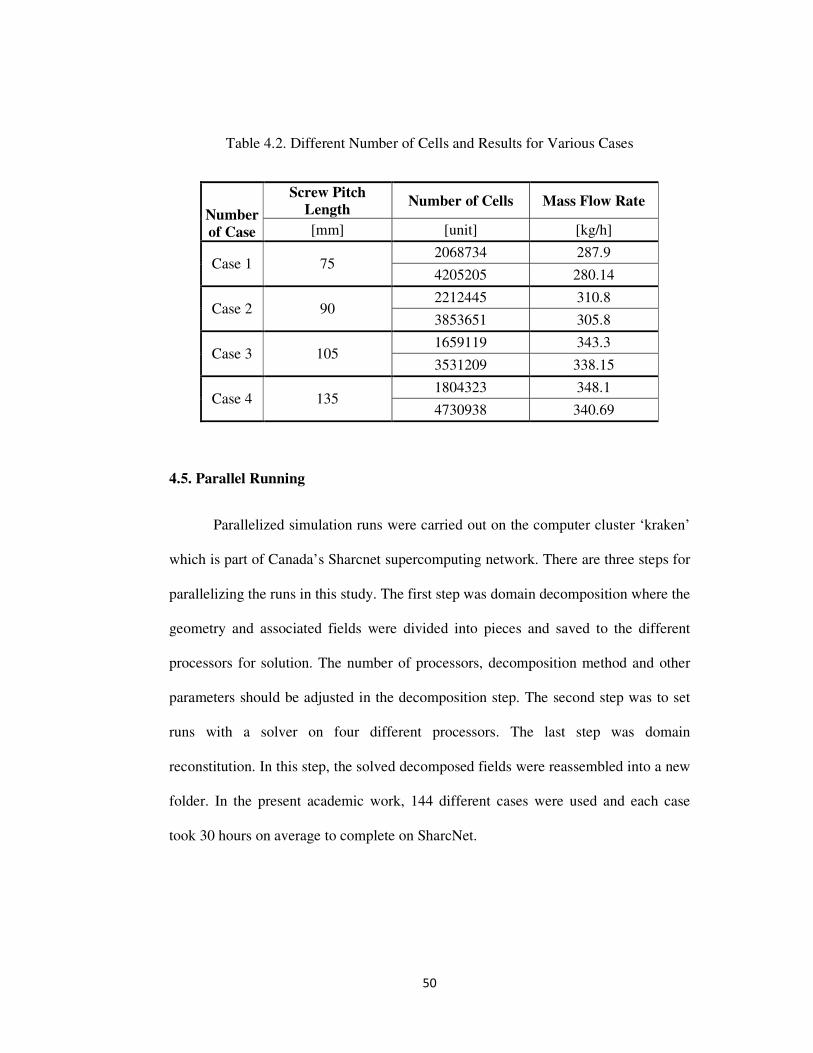
Table 4.2. Different Number of Cells and Results for Various Cases
Number
of Case
Screw Pitch
Length Number of Cells Mass Flow Rate
[mm] [unit] [kg/h]
Case 1 75 2068734 287.9
4205205 280.14
Case 2 90 2212445 310.8
3853651 305.8
Case 3 105 1659119 343.3
3531209 338.15
Case 4 135 1804323 348.1
4730938 340.69
4.5. Parallel Running
Parallelized simulation runs were carried out on the computer cluster ‘kraken’
which is part of Canada’s Sharcnet supercomputing network. There are three steps for
parallelizing the runs in this study. The first step was domain decomposition where the
geometry and associated fields were divided into pieces and saved to the different
processors for solution. The number of processors, decomposition method and other
parameters should be adjusted in the decomposition step. The second step was to set
runs with a solver on four different processors. The last step was domain
reconstitution. In this step, the solved decomposed fields were reassembled into a new
folder. In the present academic work, 144 different cases were used and each case
took 30 hours on average to complete on SharcNet.
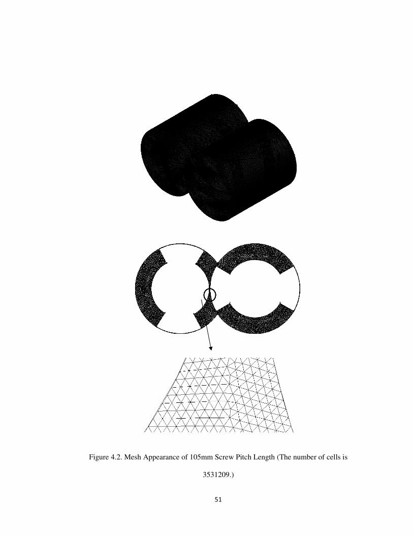
51
Figure 4.2. Mesh Appearance of 105mm Screw Pitch Length (The number of cells is
3531209.)
52
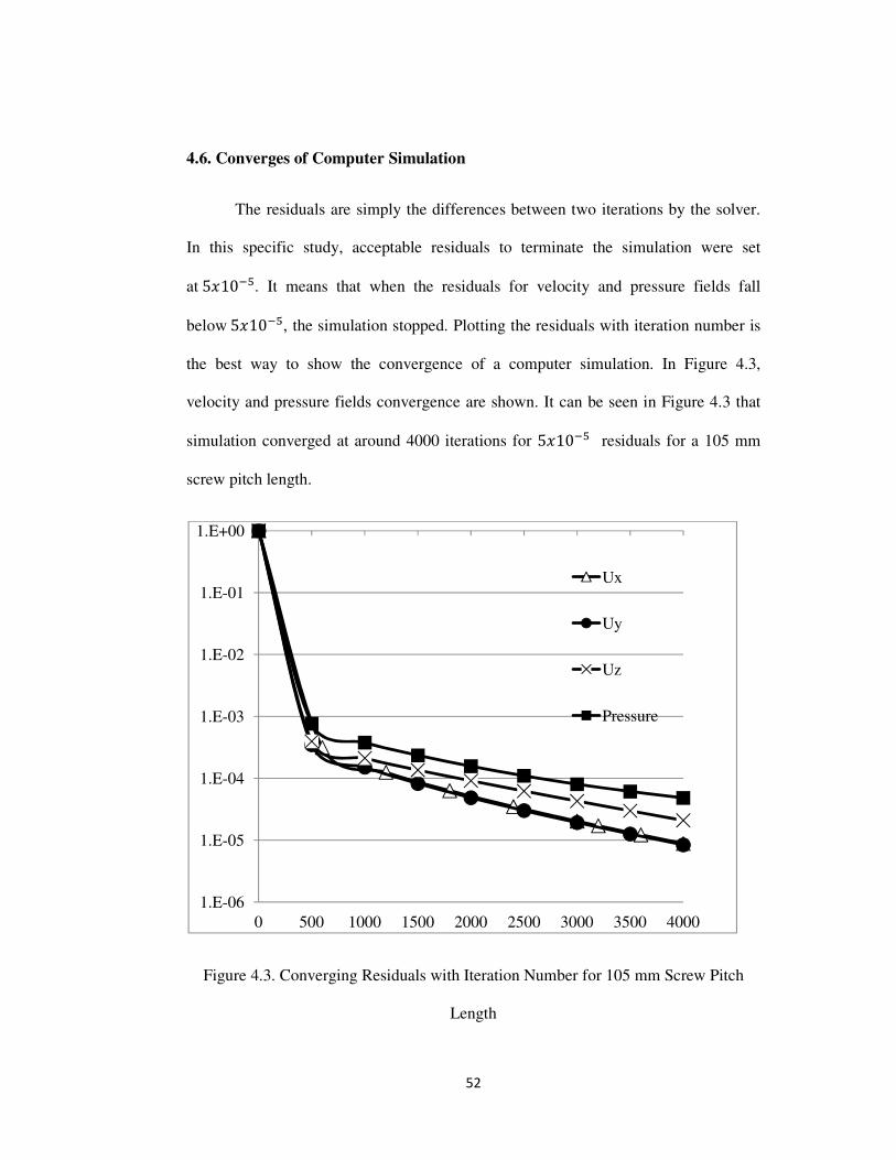
4.6. Converges of Computer Simulation
The residuals are simply the differences between two iterations by the solver.
In this specific study, acceptable residuals to terminate the simulation were set
at5q10�{. It means that when the residuals for velocity and pressure fields fall
below5q10�{, the simulation stopped. Plotting the residuals with iteration number is
the best way to show the convergence of a computer simulation. In Figure 4.3,
velocity and pressure fields convergence are shown. It can be seen in Figure 4.3 that
simulation converged at around 4000 iterations for 5q10�{ residuals for a 105 mm
screw pitch length.
Figure 4.3. Converging Residuals with Iteration Number for 105 mm Screw Pitch
Length
1.E-06
1.E-05
1.E-04
1.E-03
1.E-02
1.E-01
1.E+00
0 500 1000 1500 2000 2500 3000 3500 4000
Ux
Uy
Uz
Pressure
53
Chapter Five
NEGATIVE PRESSURE IN MODELLING ROTATING POLYMER
PROCESSING MACHINERY
5.1. Introduction
Rotating polymer processing machinery frequently involves melt flow between
two non-parallel surfaces. The melt is usually dragged and compressed towards a
narrow gap and then it expands. As a result of the drag flow in the non-parallel narrow
gap, the pressure reaches a maximum in the compression region and then a minimum
in the expansion region. Modelling is usually carried out with the help of the
lubrication approximation or with fully 3D momentum equations for creeping
(inertialess, viscous) flow. If the baseline pressure at both ends of the compression-
expansion flow field is zero, then negative pressures will be calculated in the
expansion region. Figure 5.1 shows positive and negative pressure development
between two co-rotating cylinders. In the counter-rotating case, both compression and
expansion are greater in magnitude than in the co-rotating case and consequently the
positive and negative pressures calculated are higher, as shown in Figure 5.2. Of
course, negative pressures are meaningless. However, with so many machines
operating at or near ambient pressure, boundary conditions at or close to zero values
are quite realistic and so these negative results should occur quite frequently in
modelling. It is argued in this chapter that these negative pressures are telling
researchers important information about their modeled environment.
54
5.2. Reviewing Modelling Results
An extensive literature search was carried out regarding the calculation and
reporting of negative pressures in flow simulations of twin screw extruders and other
types of rotating polymer processing equipment. In the vast majority of publications
there is never any mention that negative pressures were ever calculated when solving
the conservation of mass and momentum equations. It is not clear whether this was
due to the fortuitous occurrence of high baseline pressures or convenient choices of
boundary conditions.
Most papers ignore negative pressure results even though the mathematical
descriptions suggest such possibilities. These studies usually confine their discussions
to the negative and positive pressure gradients and the implications relating to forward
flow and back-mixing. This is particularly apparent when entry or exit boundary
conditions are at ambient pressure (i.e. zero gauge pressure). The fact that twin screw
extruders are frequently starve-fed poses additional difficulties, because the locations
of free surfaces are not priori known and cannot be determined by simply solving the
equations for drag induced flow and pressure development. Jiang et al. (2007) in a
modelling and experimental study of counter-rotating twin screw extruders show
positive pressure peaks emerging from, what appears to be, a zero pressure baseline
without mentioning if any negative pressures were ever calculated. Similar results on
counter-rotating twin screw extruders (positive pressure peaks only, above a zero
baseline pressure) are also reported in the book by White (1990), without any mention
of what was calculated between the positive pressure peaks. Although it is tempting to
associate the zones between zero pressure, with unfilled channel sections, there is no
55
reason for that. The filling ratio is set by the machine operator and has absolutely no
relation to what is predicted by the single fluid hydrodynamic analysis.
Valette et al. (2009) carried out simulations of fully filled co-rotating twin
screw extrusion, which gave pressures starting at zero, without explaining how the
zero pressure boundary was determined. Some papers have fortuitously worked with
boundary conditions with high enough pressures and avoided seeing negative values.
For example, Bravo et al. (2000) validated their simulations by actual experimental
data obtained from a co-rotating twin screw extruder and determined a high “peak”
and a low pressure “valley”, all above zero, because the baseline pressure was high
enough to avoid negative pressures. Still other papers show results with negative
pressures, but minimize their relevance to the model. Gupta et al. (2009) in their co-
rotating twin screw extrusion simulations reported qualitative agreement with
experiments and stated that “since the predicted pressure is zero at the exit, the
pressure in a portion of the 120/120 element conveying element near the entrance is
negative…the actual value of the predicted pressure is not important. It is the pressure
gradient which is captured by the flow equations”. Ortiz-Rodriguez (2009) showed in
a figure of his doctoral thesis with localized negative pressures along the length of a
co-rotating extruder reaching -0.5 MPa, without explaining what they meant or how
they could be obtained. Ilinca and Hetu (2012) in their numerical study of co-rotating
twin screw extruder mixing elements avoided giving an explanation regarding their
negative pressure values which reached -2 MPa, by simply stating that “the exit
pressure is taken as reference and it was fixed to 0 in the numerical simulation”. Radl
et al. (2010) in their computer simulations of a novel pelletizer having a rotor-stator
system, observed negative pressures in the flow field reaching -13 bar, but had no
56
explanation why the meaningless values were obtained. Similarly, Ishikawa et al
(2000) reported that some pressures were negative in simulations of co-rotating twin
screw extrusion with no reason given.
Uniformly raising the baseline pressure in simulating twin screw extruders
may avoid these meaningless negative values, but it is often not the appropriate
solution to obtaining correct pressure gradients. The boundary conditions at entry and
exit must carefully be chosen to produce physically meaningful results and not simply
be done to avoid values that cannot be explained.
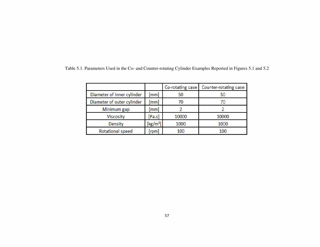
57
Table 5.1. Parameters Used in the Co- and Counter-rotating Cylinder Examples Reported in Figures 5.1 and 5.2
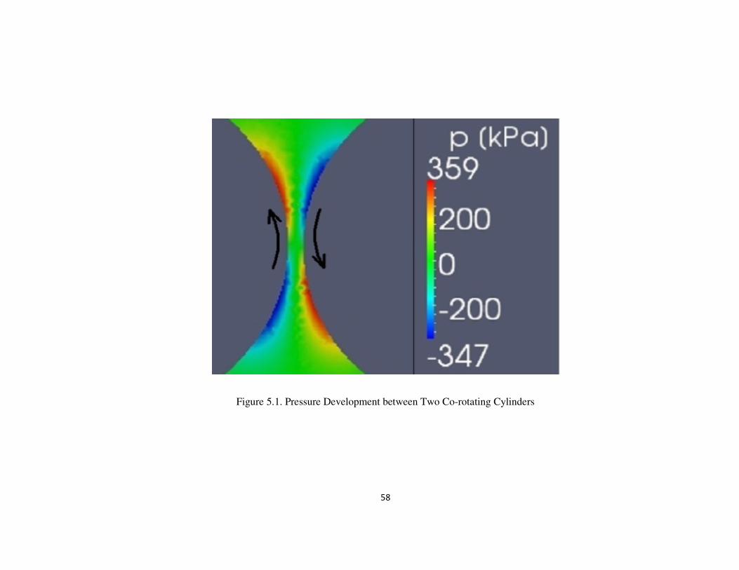
58
Figure 5.1. Pressure Development between Two Co-rotating Cylinders
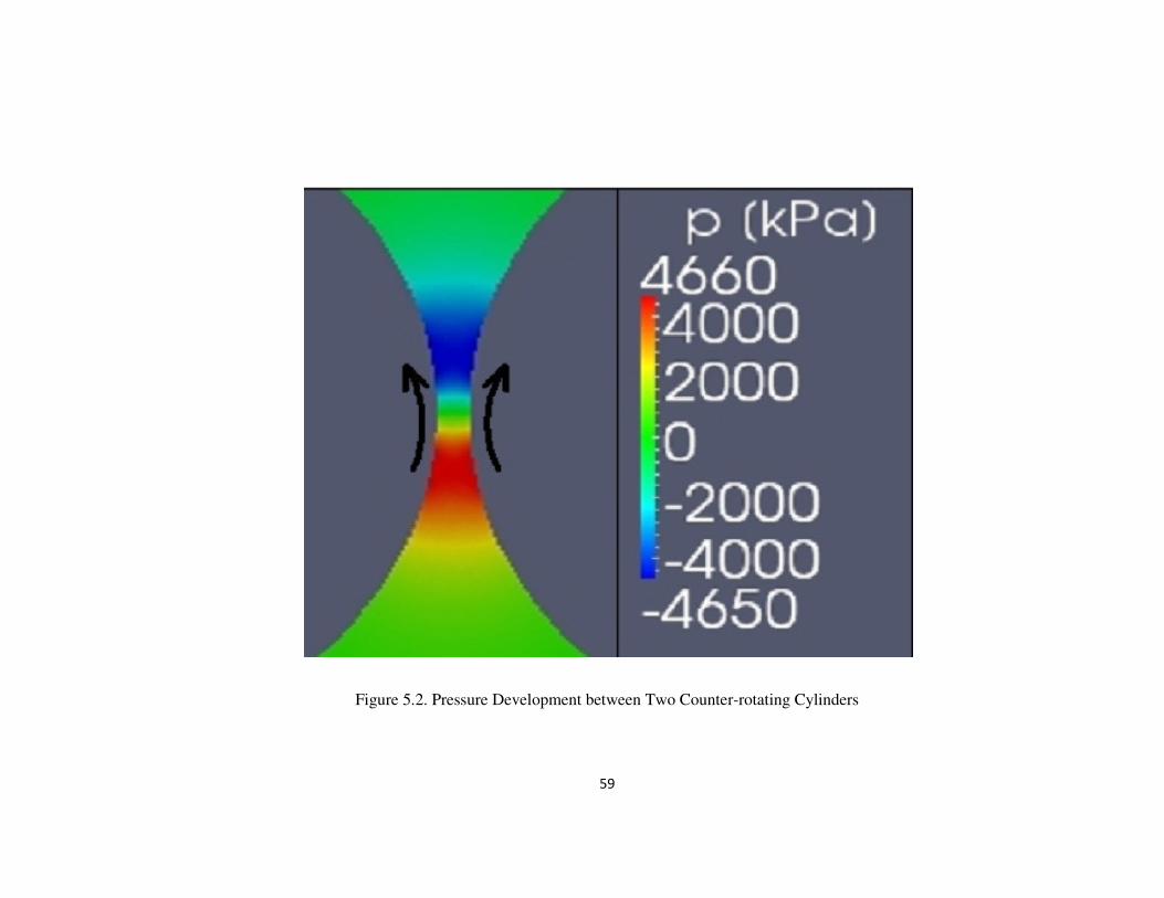
59
Figure 5.2. Pressure Development between Two Counter-rotating Cylinders
60
5.3. Explaining the Phenomenon
The non-physical result of negative pressures has been observed and properly
interpreted as to its cause for more than a hundred years in the modelling of journal
bearing lubrication. An example of such modeling results is shown in Figure 5.3. The
results were obtained using the OpenFOAM® software package for a fluid having
viscosity of 1 Pa.s, density of 1000 kg/m3, inner cylinder diameter of 40 mm rotating
at 3000 rpm, outer cylinder diameter of 41 mm and a minimum gap of 0.2 mm. It is
well recognized in the field of lubrication that in the expansion region, when the
pressure becomes less than the vapor pressure of the lubricant and/or the saturation
state of any dissolved gases, bubbles are actually forming and cavitation is taking
place, as explained in a review by Dowson and Taylor (1979) and more recently by
Gonzales-Avila et al. (2011). Of course, in the liquid-vapor region of the expansion,
the single liquid flow modelling is no longer valid. Due to the highly localized regions
where negative pressures are often reported (i.e in the nip regions of extrusion
machinery), being far from barrel walls, such findings of bubbling are difficult to
verify. But then the purpose of such modelling efforts is often to observe and explain
phenomena inside the process that cannot be physically observed by the conventional
placement of sensors. We are inferring that modellers of polymer systems within
rotating machinery simply need to recognize that their negative results may be an
indication of a multiphasic system being incorrectly reconciled within a single phase
model.
We do not mean to infer from our statements above that observing negative
pressure results invalidates the relevance of the model. In most cases, the flow regions
61
showing negative values occupy a small portion of the overall system. However, they
should be reported as they may lead to future studies with more complex phase
assumptions being introduced.
5.4. Conclusion
Negative pressures obtained in modelling of rotating polymer processing
machinery indicate the possibility of local bubble formation and cavitation, when the
pressure drops below the vapor pressure of dissolved gases, as it is well known in
journal bearing lubrication. The single fluid modelling is not valid in such flow
regions. When simulations are carried out, the baseline pressure, which would
prevent the meaningless negative pressures, should be clearly stated and its impact on
pressure gradients and any conclusions relating to mixing or scale-up should be
discussed. The purpose of numerical simulation is to produce results, which should
reflect reality and could be confirmed by experimental measurements of several
quantities, including pressures.
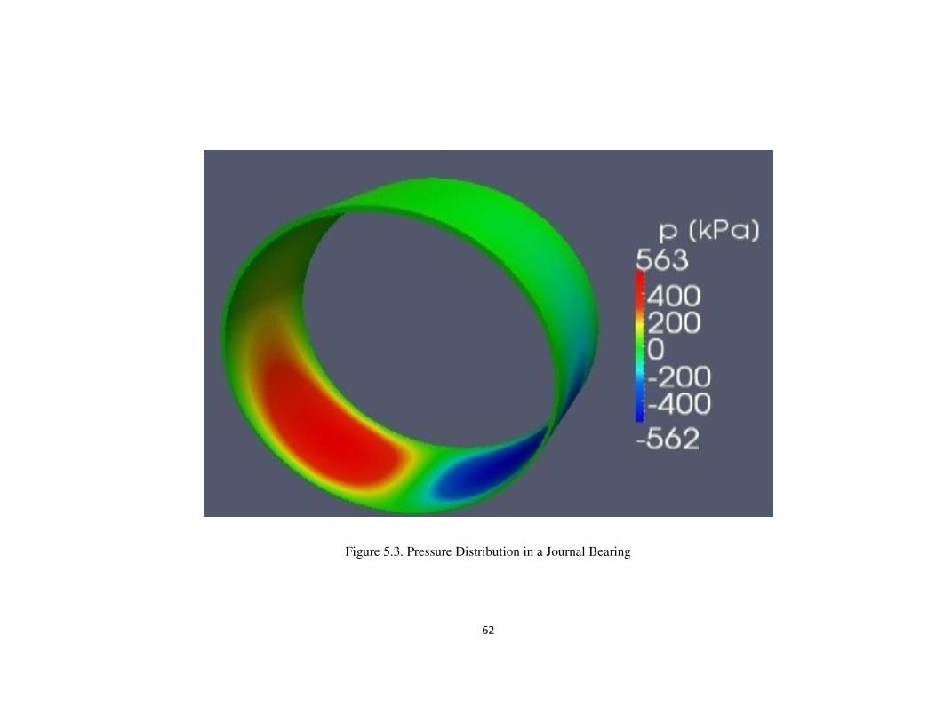
62
Figure 5.3. Pressure Distribution in a Journal Bearing
63
Chapter Six
NUMERICAL RESULTS
6.1. Introduction
Generally, twin screw extruders are divided into three zones: solid conveying
zone, melting zone and metering zone. In metering zone, all the particles of polymer
are at molten phase. Ideally, all screw channels are filled with molten polymer in this
region. Since pumping and mixing mainly take place in metering zone, it is very
important to characterize the metering region to understand the twin screw extruder
process.
The purpose of this study is to investigate the pumping behaviour and mixing
performance of metering zone of intermeshing counter rotating twin screw extruders
(ICRTSE) for various screw pitch lengths, flight width-to-channel width ratios and
screw speeds. Pumping behaviour and dispersive mixing ability of ICRTSE provide
information screw designers and operators for better understanding of both screw
geometries and processing conditions.
6.2. Description of Method
One of the biggest challenges in simulating ICRTSE is the time dependent
flow boundaries as the screws rotate in counter direction. Lee and Castro (1989)
mentioned that some extrusion processes cannot reach a truly steady state due to the
start-end-repeat behaviour in polymer processing. If the Reynolds number is very
small, time dependency at flow boundaries are negligible compared to other terms in
the equations of motion. With this assumption, extrusion processes can only reach a
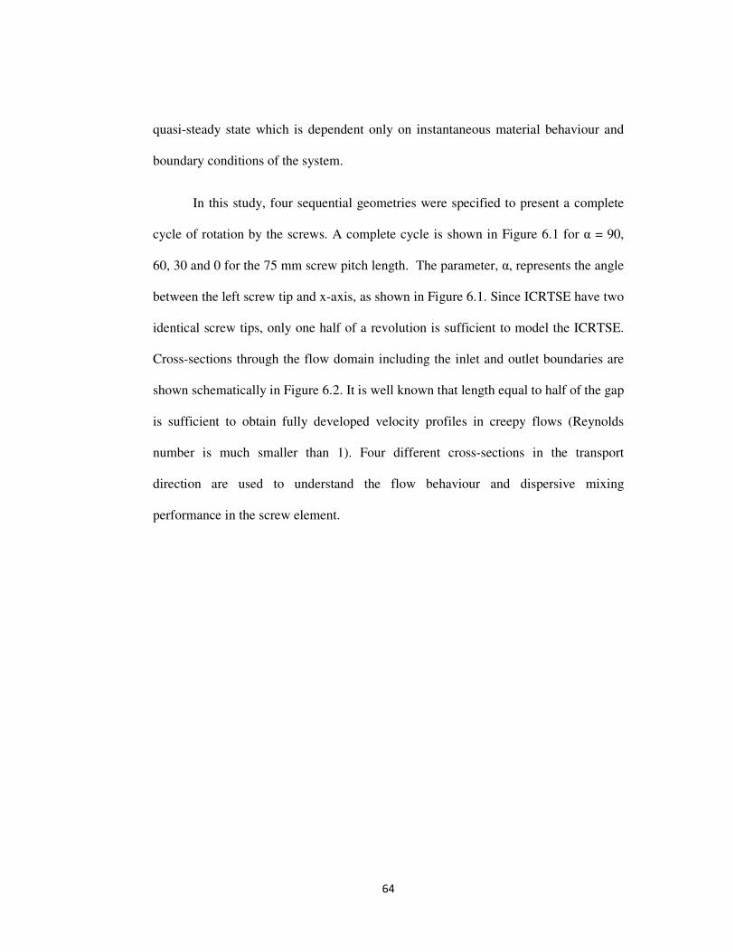
64
quasi-steady state which is dependent only on instantaneous material behaviour and
boundary conditions of the system.
In this study, four sequential geometries were specified to present a complete
cycle of rotation by the screws. A complete cycle is shown in Figure 6.1 for α = 90,
60, 30 and 0 for the 75 mm screw pitch length. The parameter, α, represents the angle
between the left screw tip and x-axis, as shown in Figure 6.1. Since ICRTSE have two
identical screw tips, only one half of a revolution is sufficient to model the ICRTSE.
Cross-sections through the flow domain including the inlet and outlet boundaries are
shown schematically in Figure 6.2. It is well known that length equal to half of the gap
is sufficient to obtain fully developed velocity profiles in creepy flows (Reynolds
number is much smaller than 1). Four different cross-sections in the transport
direction are used to understand the flow behaviour and dispersive mixing
performance in the screw element.
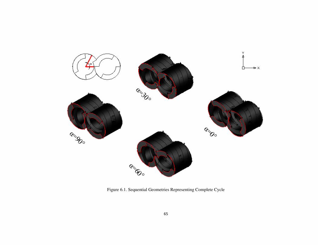
65
Figure 6.1. Sequential Geometries Representing Complete Cycle
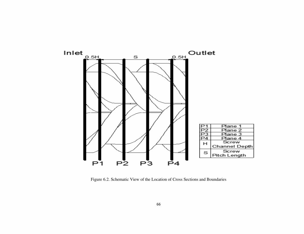
66
Figure 6.2. Schematic View of the Location of Cross Sections and Boundaries
67
6.3. Flow Pattern in ICRTSE
In this section, the axial velocities and pumping efficiency are investigated to
understand the flow behaviour of ICRTSE. Different screw pitch lengths, flight width-
to-channel width ratios, power indexes and screw speeds were used to study the screw
geometries and processing conditions of an ICRTSE.
6.3.1. Axial Velocity in ICRTSE
Axial velocity is one of the most important parameters to understanding the
flow behaviour of an ICRTSE. Axial velocity is the main component of velocity in the
transport direction of flow. Axial velocities are shown in Figure 6.3 to 6.6 for various
cross sections for 105 mm screw pitch length. The positive value in these figures
correspond to the flow in the transport direction whereas negative values indicate that
the flow in the opposite transport direction. Figure 6.3 to 6.6 reveal that most of the
polymers flow was in the transport direction.
The results indicated that the maximum positive axial velocity occurred before
the converging section of intermeshing region and screw tips while the maximum
negative axial velocity occurred in the intermeshing region. In fact, most of the fluid
in the intermeshing region exhibited negative axial velocity values. Shah and Gupta
(2004) found that the maximum axial velocity occurred in a similar location as the
present results for their 29.2 mm diameter ICTRSE simulations and likewise, included
mention that the axial velocity was predominantly backwards in their intermeshing
region. Similarly, Ma et al. (2004) noted negative velocity values in their simulation
results for the intermeshing region of a 33.2 mm diameter ICRTSE.
68
The average values for axial velocities of all four different geometries in a
complete cycle are shown in Tables 6.1 to 6.3 for power index values of 1, 0.7 and 0.3
respectively. These averages were calculated by weighing the axial velocity for each
element by the area of the element itself across the entire cross section. It is noted that
the average values hardly ever change from one geometry to another for the same
screw pitch length. Thus, it is shown in Tables 6.1 to 6.3 that one angle for α is
sufficient to use for flow rate determination of ICRTSE with fully agreement Li and
Manas-Zloczower (1994). It can be seen from Tables 6.1 to 6.3 that the average axial
velocity decreased with increasing screw pitch length. Since lower power index fluid
has a smaller viscosity at the same shear rate which cause higher leakage flows, the
average axial velocity goes down with shear thinning.

69
Table 6.1. Average Axial Velocities for Various α and for Screw Pitch Length for
Power Index 1
Screw Pitch Length Average Axial
Velocity
[mm] [mm/s]
75 mm Screw Pitch
Length
α=90° 16.12
α=60° 16.33
α=30° 16.27
α=0° 16.08
90 mm Screw Pitch
Length
α=90° 15.64
α=60° 15.79
α=30° 15.77
α=0° 15.61
105 mm Screw Pitch
Length
α=90° 15.18
α=60° 15.22
α=30° 15.24
α=0° 15.14
135 mm Screw Pitch
Length
α=90° 14.13
α=60° 14.38
α=30° 14.27
α=0° 14.14
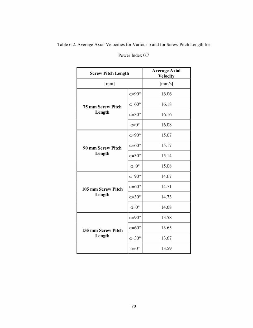
70
Table 6.2. Average Axial Velocities for Various α and for Screw Pitch Length for
Power Index 0.7
Screw Pitch Length Average Axial
Velocity
[mm] [mm/s]
75 mm Screw Pitch
Length
α=90° 16.06
α=60° 16.18
α=30° 16.16
α=0° 16.08
90 mm Screw Pitch
Length
α=90° 15.07
α=60° 15.17
α=30° 15.14
α=0° 15.08
105 mm Screw Pitch
Length
α=90° 14.67
α=60° 14.71
α=30° 14.73
α=0° 14.68
135 mm Screw Pitch
Length
α=90° 13.58
α=60° 13.65
α=30° 13.67
α=0° 13.59

71
Table 6.3. Average Axial Velocities for Various α and for Screw Pitch Length for
Power Index 0.3
Screw Pitch Length Average Axial
Velocity
[mm] [mm/s]
75 mm Screw Pitch
Length
α=90° 13.66
α=60° 13.65
α=30° 13.62
α=0° 13.66
90 mm Screw Pitch
Length
α=90° 13.05
α=60° 13.07
α=30° 13.11
α=0° 13.05
105 mm Screw Pitch
Length
α=90° 12.49
α=60° 12.51
α=30° 12.53
α=0° 12:50
135 mm Screw Pitch
Length
α=90° 11.98
α=60° 12.01
α=30° 12.05
α=0° 11.97
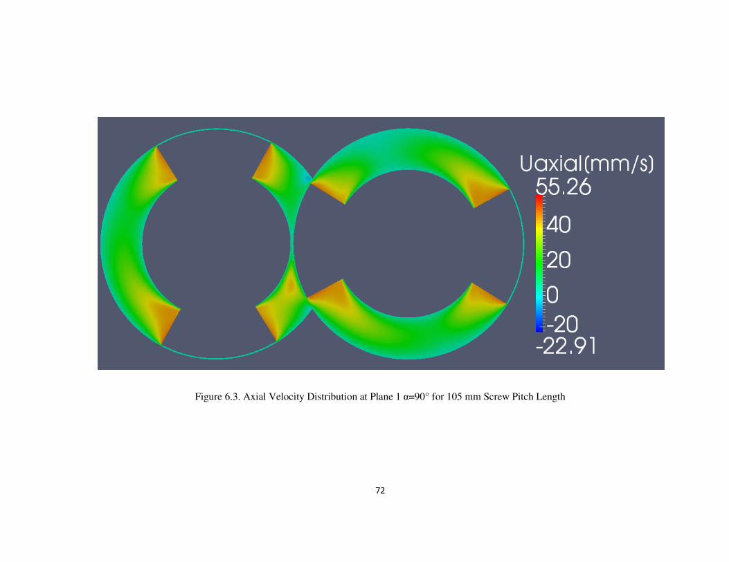
72
Figure 6.3. Axial Velocity Distribution at Plane 1 α=90° for 105 mm Screw Pitch Length
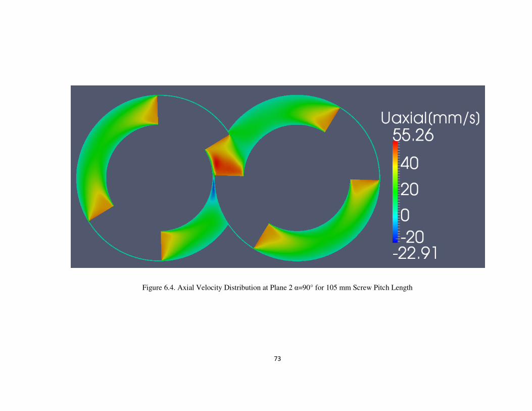
73
Figure 6.4. Axial Velocity Distribution at Plane 2 α=90° for 105 mm Screw Pitch Length
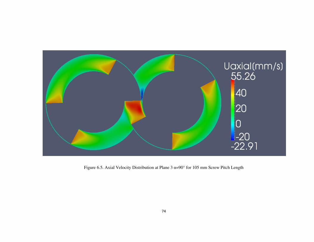
74
Figure 6.5. Axial Velocity Distribution at Plane 3 α=90° for 105 mm Screw Pitch Length
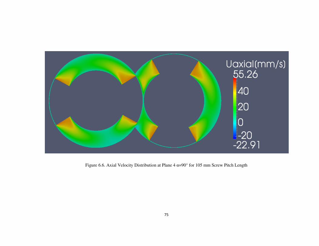
75
Figure 6.6. Axial Velocity Distribution at Plane 4 α=90° for 105 mm Screw Pitch Length
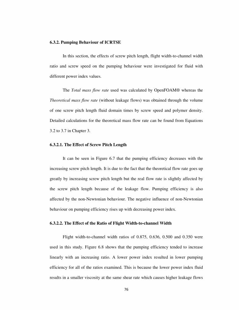
76
6.3.2. Pumping Behaviour of ICRTSE
In this section, the effects of screw pitch length, flight width-to-channel width
ratio and screw speed on the pumping behaviour were investigated for fluid with
different power index values.
The Total mass flow rate used was calculated by OpenFOAM® whereas the
Theoretical mass flow rate (without leakage flows) was obtained through the volume
of one screw pitch length fluid domain times by screw speed and polymer density.
Detailed calculations for the theoretical mass flow rate can be found from Equations
3.2 to 3.7 in Chapter 3.
6.3.2.1. The Effect of Screw Pitch Length
It can be seen in Figure 6.7 that the pumping efficiency decreases with the
increasing screw pitch length. It is due to the fact that the theoretical flow rate goes up
greatly by increasing screw pitch length but the real flow rate is slightly affected by
the screw pitch length because of the leakage flow. Pumping efficiency is also
affected by the non-Newtonian behaviour. The negative influence of non-Newtonian
behaviour on pumping efficiency rises up with decreasing power index.
6.3.2.2. The Effect of the Ratio of Flight Width-to-channel Width
Flight width-to-channel width ratios of 0.875, 0.636, 0.500 and 0.350 were
used in this study. Figure 6.8 shows that the pumping efficiency tended to increase
linearly with an increasing ratio. A lower power index resulted in lower pumping
efficiency for all of the ratios examined. This is because the lower power index fluid
results in a smaller viscosity at the same shear rate which causes higher leakage flows

77
and lower pumping efficiency. In addition, the effect of power index on pumping
efficiency increases with decreasing power index value. It is concluded that thick
flighted elements have a greater pumping ability than thin flighted elements.
6.3.2.3. The Effect of Screw Speed
Screw speed has already been mentioned to be one of the most crucial
processing parameters in terms of pumping behaviour for the ICRTSE. Speeds of 30,
60, and 120 rpm were investigated. Figures 6.9, 6.10 and 6.11 indicate that the
influence of screw speed on pumping efficiency is almost negligible similar to the
findings with the simple model. It is concluded that screw speed affects the theoretical
flow rate and total flow rate at same degree.
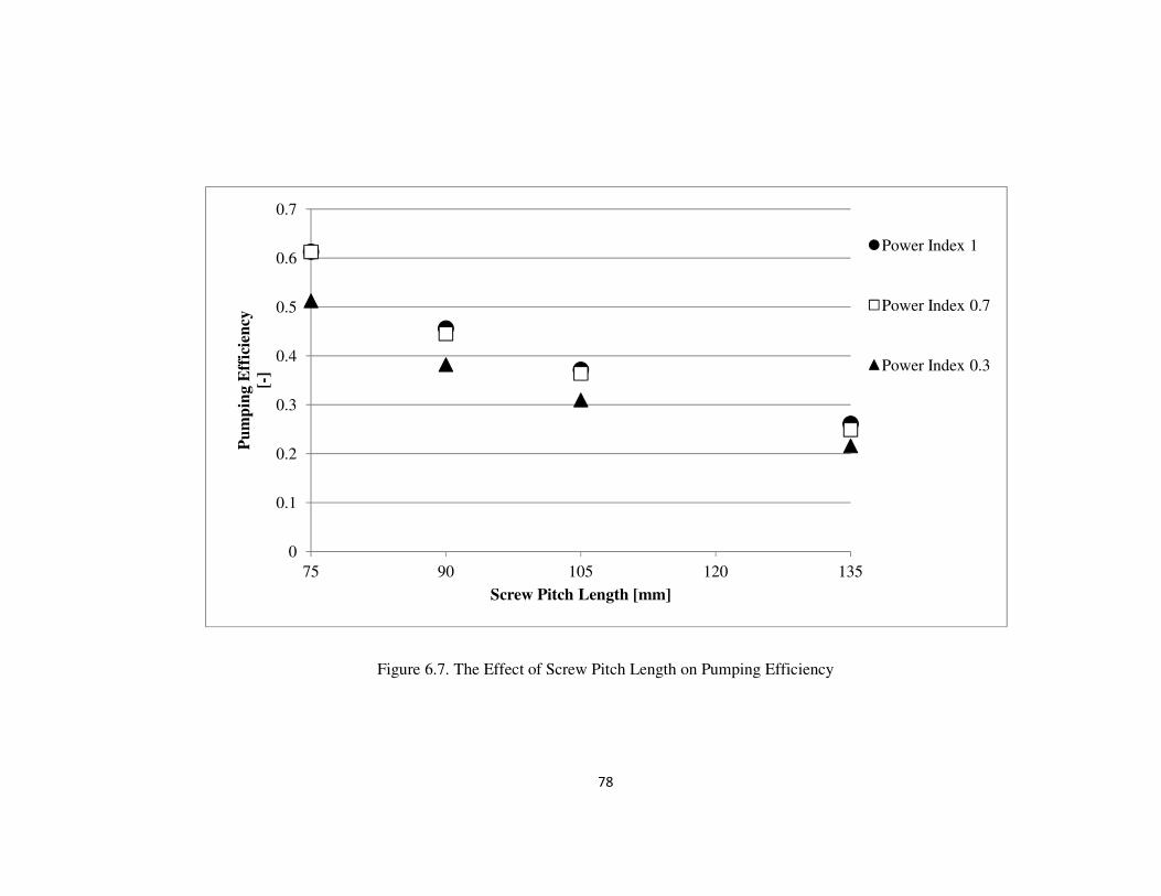
78
Figure 6.7. The Effect of Screw Pitch Length on Pumping Efficiency
0
0.1
0.2
0.3
0.4
0.5
0.6
0.7
75 90 105 120 135
Pu
mp
ing
Eff
icie
ncy
[-]
Screw Pitch Length [mm]
Power Index 1
Power Index 0.7
Power Index 0.3
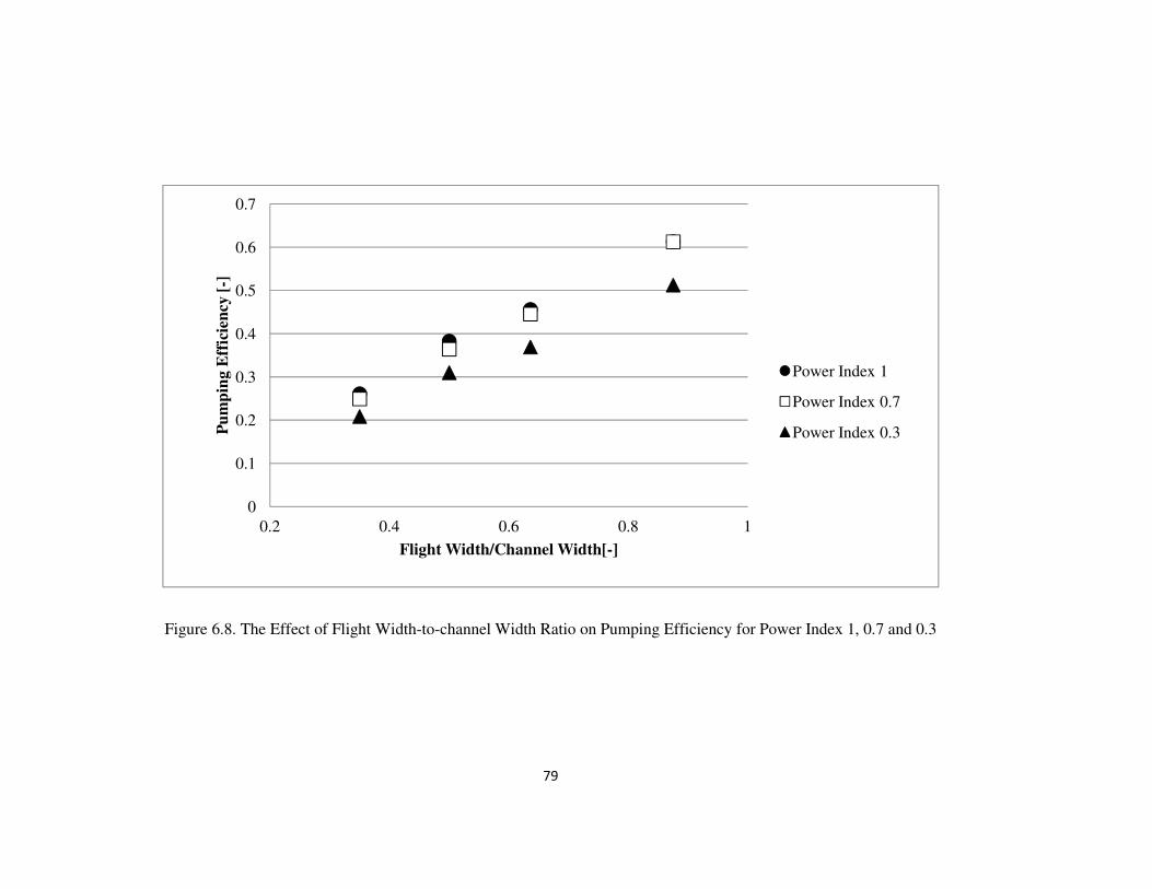
79
Figure 6.8. The Effect of Flight Width-to-channel Width Ratio on Pumping Efficiency for Power Index 1, 0.7 and 0.3
0
0.1
0.2
0.3
0.4
0.5
0.6
0.7
0.2 0.4 0.6 0.8 1
Pu
mp
ing E
ffic
ien
cy [
-]
Flight Width/Channel Width[-]
Power Index 1
Power Index 0.7
Power Index 0.3
80
Figure 6.9. The Effect of Screw Speed on Pumping Efficiency for Power Index 1
0
0.1
0.2
0.3
0.4
0.5
0.6
0.7
20 30 40 50 60 70 80 90 100 110 120
Pu
mp
ing
Eff
icie
ncy
[-]
Screw Speed [rpm]
75mm
90mm
105mm
135mm
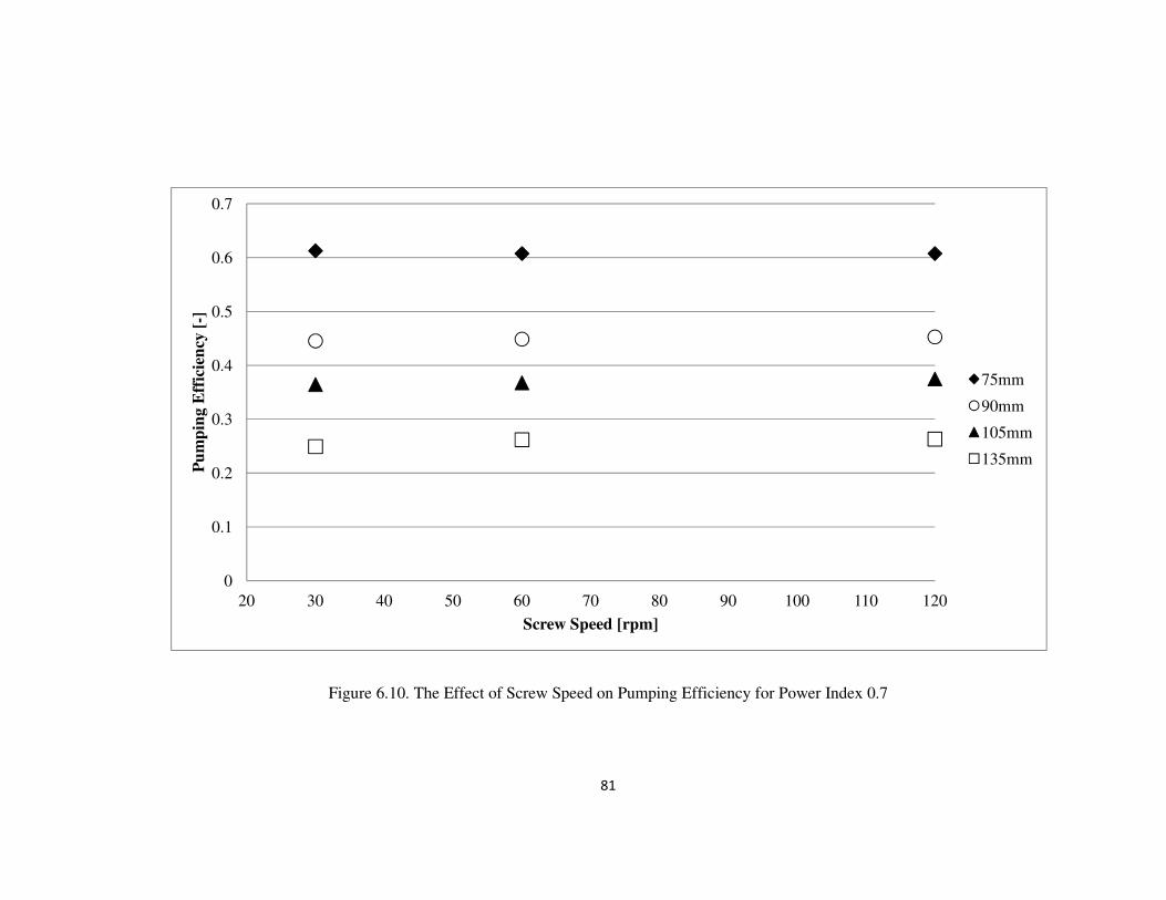
81
Figure 6.10. The Effect of Screw Speed on Pumping Efficiency for Power Index 0.7
0
0.1
0.2
0.3
0.4
0.5
0.6
0.7
20 30 40 50 60 70 80 90 100 110 120
Pu
mp
ing
Eff
icie
ncy
[-]
Screw Speed [rpm]
75mm
90mm
105mm
135mm
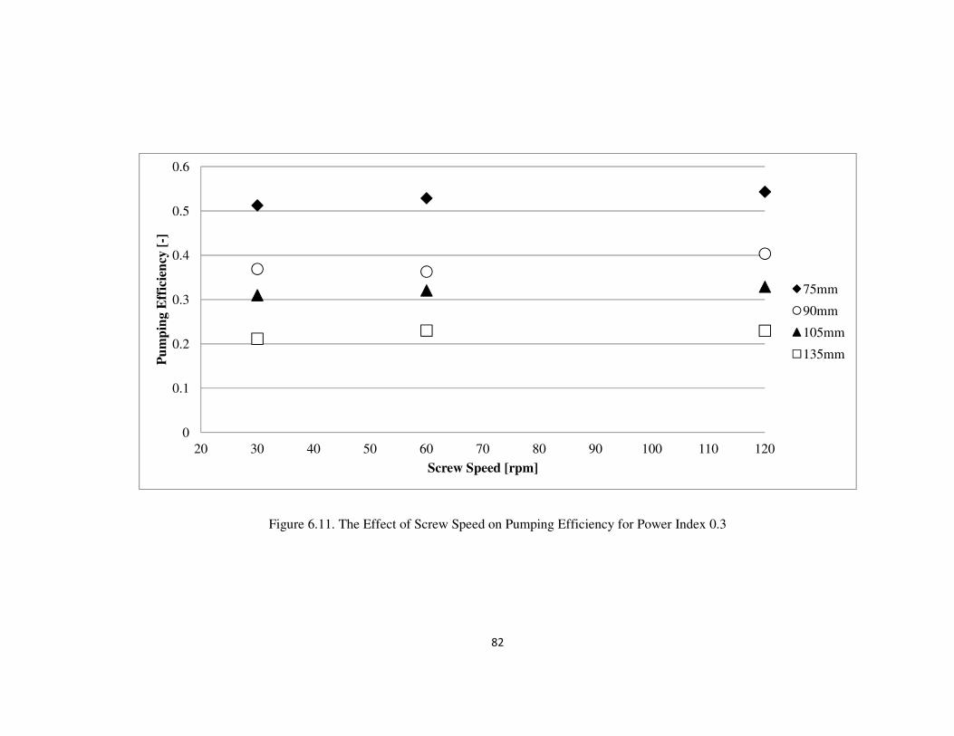
82
Figure 6.11. The Effect of Screw Speed on Pumping Efficiency for Power Index 0.3
0
0.1
0.2
0.3
0.4
0.5
0.6
20 30 40 50 60 70 80 90 100 110 120
Pu
mp
ing
Eff
icie
ncy
[-]
Screw Speed [rpm]
75mm
90mm
105mm
135mm
83
6.4. Dispersive Mixing Behaviour of ICRTSE
Quantification of mixing is always challenging in polymer processing. More is
the norm is to talk about mixing in terms of ‘good’ versus ‘bad’. To interpret the
dispersive mixing efficiency of ICRTSE, both the shear stress distribution and
dispersive mixing parameter, λ, were used in this analysis. Mixing parameter λ was
defined by Manas-Zloczower et al. (1988, 1989) as in Equations 6.2 to 6.5.
Kajiwara et al. (1996) mentioned that knowing the shear stress distribution of a
process was a valuable measure to evaluating the dispersive mixing of a twin screw
extruder. Yang (1993) used shear stress distribution and mixing parameter λ to
understand the dispersive mixing behaviour of batch mixer and co-rotating twin screw
extruder. Similarly, Li and Manas-Zloczower (1994) investigated the influence of
screw speed and axial pressure difference on dispersive mixing for a 34 mm diameter
counter-rotating twin screw extruder. They focus on both shear stress distribution and
mixing parameter λ as well to quantify the dispersive mixing.
6.4.1. Shear Stress Distribution
Shear stress distributions are shown from Figures 6.12 to 6.15 for various cross
sections of the conveying element with 105 mm screw pitch length and power index
of 0.7. The distributions indicate that the maximum shear stress was always at the
screw tips (the region between screw and barrel) or in the intermeshing region (the
region between screws). It is because of that fluid is forced to pass through small gaps
in these regions. The shear stress in screw tips and intermeshing region were found to
be of the same order of magnitude. In comparison, Li and Manas-Zloczower (1994)
found the same results with their simulations of a 34 mm diameter ICRTSE. Kajiwara
84
et al. (1996) found the highest stresses only in intermeshing region for 40 mm
diameter counter rotating twin screw extruder.
The average values of the shear stress for all geometries are shown in Tables
6.4 and 6.5 for power index values of 0.7 and 0.3 respectively. The average values of
shear stresses and mixing parameter λ in Tables 6.4 and 6.5 were calculated by
following the method of Yang and Manas-Zloczower (1992). They were calculated by
weighing the corresponding parameters for each cell by the volume of the cell itself. It
is noted from the tables that the average values hardly ever change from one geometry
to another for the same screw pitch length. As a result, similar to axial velocity
determination, it is concluded that one angle for α is sufficient to use for shear stress
and mixing parameter λ determination of ICRTSE which is in agreement with Li and
Manas-Zloczower (1994). It is seen in Tables 6.4 and 6.5 that average shear stress
decreased with increasing screw pitch length. This was due to the fact that
intermeshing region became smaller with increasing screw pitch length. Average
shear stress dropped dramatically with decreasing power index, as expected.
The shear stress distributions in Figures 6.16 to 6.19 correspond to the
conveying elements with 75 mm and 105 mm screw pitch lengths were determined for
power indexes of 0.7 and 0.3 respectively. It can be seen in Figures 6.16 and 6.17 that
shear stress distribution becomes slightly narrower with increasing screw pitch length.
In addition, the shear rate distribution becomes wider while the power index decreased
in Figures 6.18 and 6.19.

85
The effects of screw speeds on the shear stress distribution are shown in
Figures 6.20 and 6.21 for power indexes of 0.7 and 0.3. Average shear stress values
over the geometry showed less differences as the power index decreased from 0.7 to
0.3.
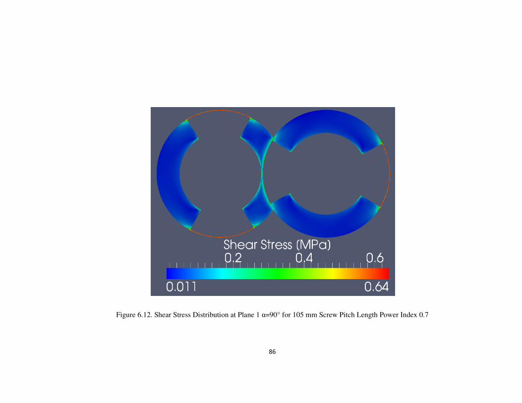
86
Figure 6.12. Shear Stress Distribution at Plane 1 α=90° for 105 mm Screw Pitch Length Power Index 0.7
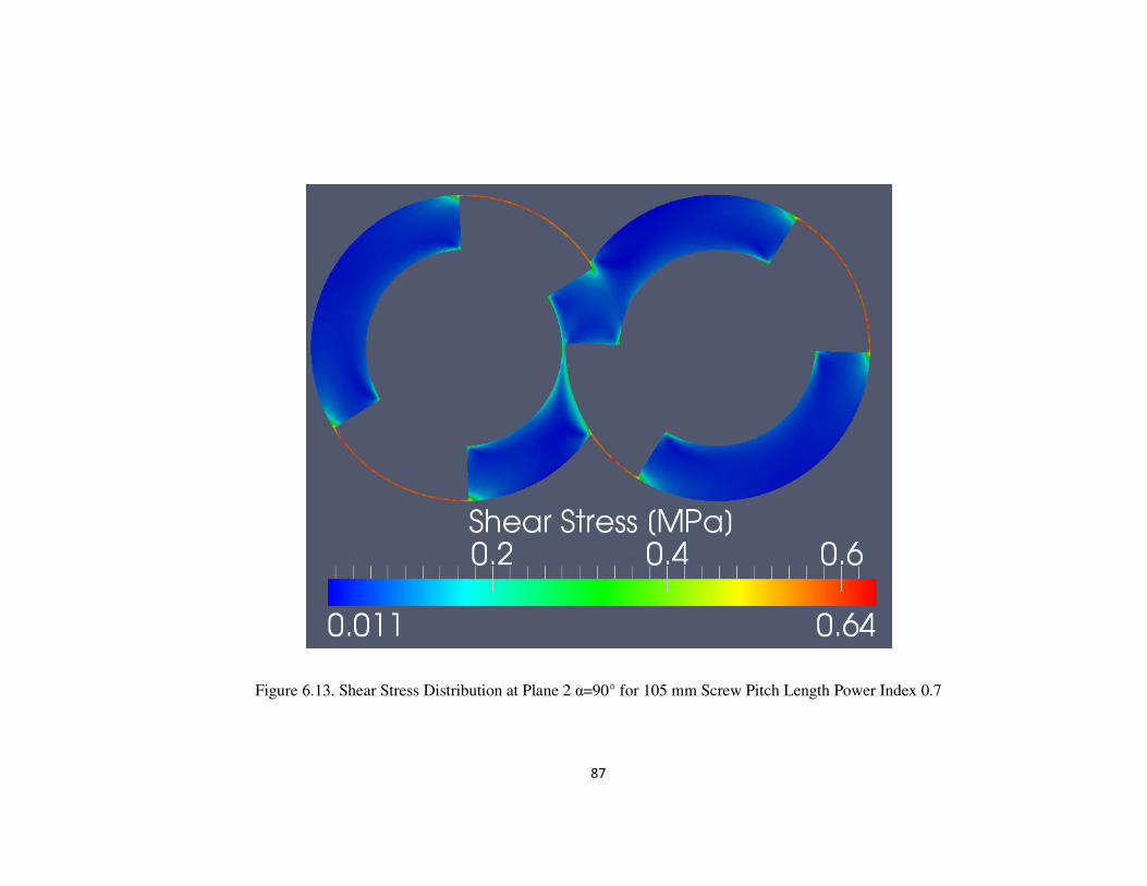
87
Figure 6.13. Shear Stress Distribution at Plane 2 α=90° for 105 mm Screw Pitch Length Power Index 0.7
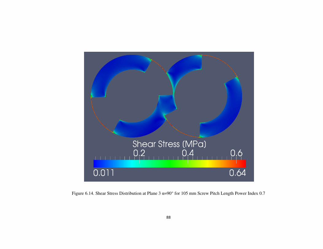
88
Figure 6.14. Shear Stress Distribution at Plane 3 α=90° for 105 mm Screw Pitch Length Power Index 0.7
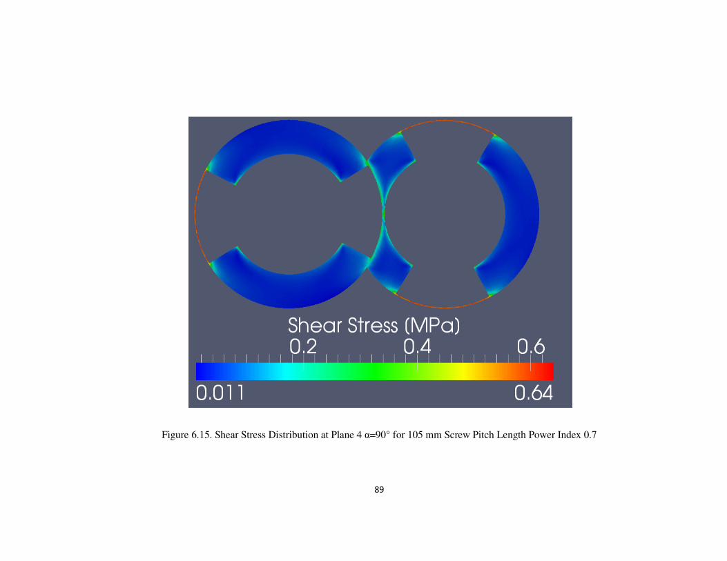
89
Figure 6.15. Shear Stress Distribution at Plane 4 α=90° for 105 mm Screw Pitch Length Power Index 0.7
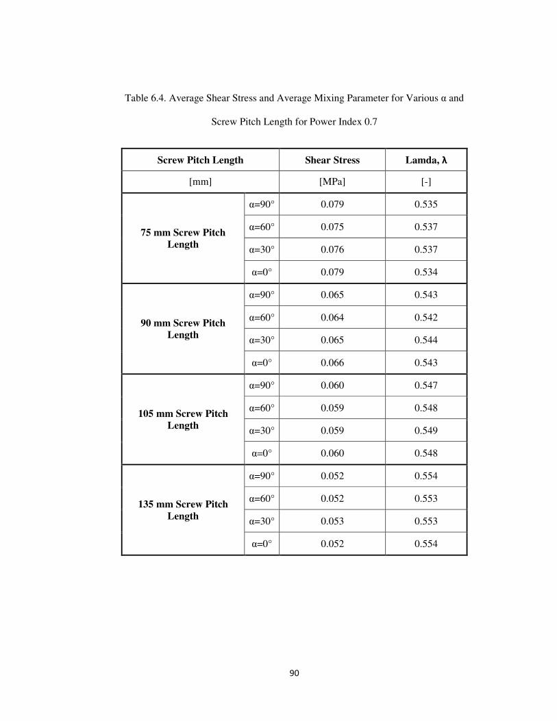
90
Table 6.4. Average Shear Stress and Average Mixing Parameter for Various α and
Screw Pitch Length for Power Index 0.7
Screw Pitch Length Shear Stress Lamda, λ
[mm] [MPa] [-]
75 mm Screw Pitch
Length
α=90° 0.079 0.535
α=60° 0.075 0.537
α=30° 0.076 0.537
α=0° 0.079 0.534
90 mm Screw Pitch
Length
α=90° 0.065 0.543
α=60° 0.064 0.542
α=30° 0.065 0.544
α=0° 0.066 0.543
105 mm Screw Pitch
Length
α=90° 0.060 0.547
α=60° 0.059 0.548
α=30° 0.059 0.549
α=0° 0.060 0.548
135 mm Screw Pitch
Length
α=90° 0.052 0.554
α=60° 0.052 0.553
α=30° 0.053 0.553
α=0° 0.052 0.554
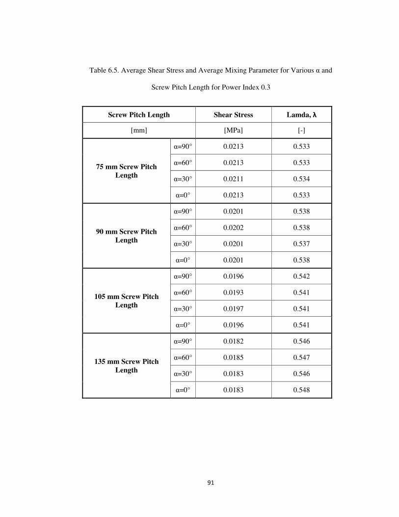
91
Table 6.5. Average Shear Stress and Average Mixing Parameter for Various α and
Screw Pitch Length for Power Index 0.3
Screw Pitch Length Shear Stress Lamda, λ
[mm] [MPa] [-]
75 mm Screw Pitch
Length
α=90° 0.0213 0.533
α=60° 0.0213 0.533
α=30° 0.0211 0.534
α=0° 0.0213 0.533
90 mm Screw Pitch
Length
α=90° 0.0201 0.538
α=60° 0.0202 0.538
α=30° 0.0201 0.537
α=0° 0.0201 0.538
105 mm Screw Pitch
Length
α=90° 0.0196 0.542
α=60° 0.0193 0.541
α=30° 0.0197 0.541
α=0° 0.0196 0.541
135 mm Screw Pitch
Length
α=90° 0.0182 0.546
α=60° 0.0185 0.547
α=30° 0.0183 0.546
α=0° 0.0183 0.548
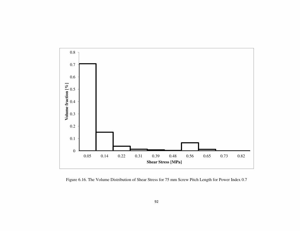
92
Figure 6.16. The Volume Distribution of Shear Stress for 75 mm Screw Pitch Length for Power Index 0.7
0
0.1
0.2
0.3
0.4
0.5
0.6
0.7
0.8
0.05 0.14 0.22 0.31 0.39 0.48 0.56 0.65 0.73 0.82
Vo
lum
e fr
act
ion
[%
]
Shear Stress [MPa]
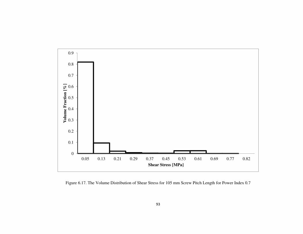
93
Figure 6.17. The Volume Distribution of Shear Stress for 105 mm Screw Pitch Length for Power Index 0.7
0
0.1
0.2
0.3
0.4
0.5
0.6
0.7
0.8
0.9
0.05 0.13 0.21 0.29 0.37 0.45 0.53 0.61 0.69 0.77 0.82
Vo
lum
e F
ract
ion
[%
]
Shear Stress [MPa]
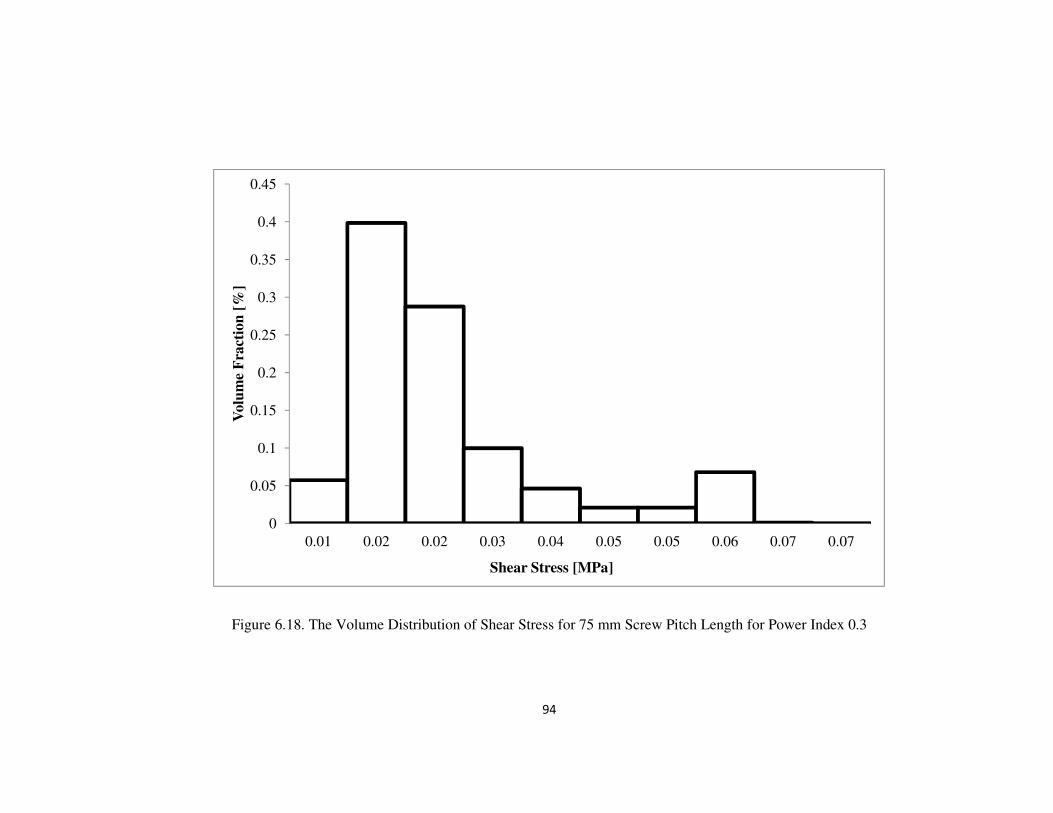
94
Figure 6.18. The Volume Distribution of Shear Stress for 75 mm Screw Pitch Length for Power Index 0.3
0
0.05
0.1
0.15
0.2
0.25
0.3
0.35
0.4
0.45
0.01 0.02 0.02 0.03 0.04 0.05 0.05 0.06 0.07 0.07
Vo
lum
e F
ract
ion
[%
]
Shear Stress [MPa]
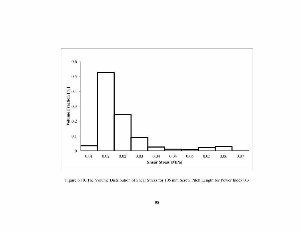
95
Figure 6.19. The Volume Distribution of Shear Stress for 105 mm Screw Pitch Length for Power Index 0.3
0
0.1
0.2
0.3
0.4
0.5
0.6
0.01 0.02 0.02 0.03 0.04 0.04 0.05 0.05 0.06 0.07
Vo
lum
e F
ract
ion
[%
]
Shear Stress [MPa]
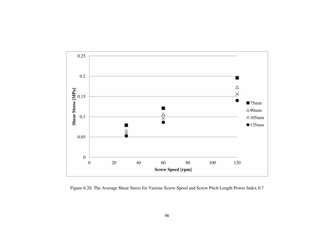
96
Figure 6.20. The Average Shear Stress for Various Screw Speed and Screw Pitch Length Power Index 0.7
0
0.05
0.1
0.15
0.2
0.25
0 20 40 60 80 100 120
Sh
ear
Str
ess
[MP
a]
Screw Speed [rpm]
75mm
90mm
105mm
135mm
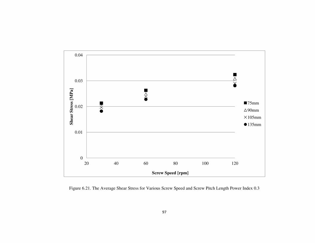
97
Figure 6.21. The Average Shear Stress for Various Screw Speed and Screw Pitch Length Power Index 0.3
0
0.01
0.02
0.03
0.04
20 40 60 80 100 120
Sh
ear
Str
ess
[MP
a]
Screw Speed [rpm]
75mm
90mm
105mm
135mm
98
6.4.2. Mixing Parameter Lamda
Manas-Zloczower et al. (1989, 1992) defined the mixing parameter, λ, as in
Equation 6.2.
) = |�|�|�|� + |}|(6.2)
�� ̿ = ∇����� + (∇V����)�(6.3)
}n = ∇����� − (∇V����)�(6.4)
|�� | = �12 (�:� �� )(6.5)
|}| = �12 |}: }|(6.5)
where |�|� is the magnitude of the rate of strain tensor and |}| is the magnitude of the
rate of vorticity tensor. �� and ω are related to the second invariants of the strain rate
tensor and vorticity tensor. λ quantifies the elongational and rotational flow which are
often thought to be more strongly relevant to dispersive mixing compared to shear. It
has a value between 0 and 1, where ) = 0 indicates pure rotation while ) = 1
indicates pure elongation and ) = 0.5 corresponds to simple shear flow. The mixing
parameter λ distribution is indicated from Figures 6.22 to 6.25 for various cross
sections of the conveying element with 105 mm screw pitch and a fluid with power
index of 0.7.
99
Li and Manas-Zloczower (1994) mentioned that simple shear flow dominated
most of the flow region of their simulated 34 mm counter-rotating twin screw
extruder. Figures 6.29 to 6.32 show that the mixing parameter λ was between 0.5 and
0.6 in most regions, indicating shear flow was dominant for this ICRTSE as well.
Figures 6.22 to 6.25 imply that the maximum λ occurs in the intermeshing region due
to a high rate of the strain tensor and low rate of the vorticity tensor. The intermeshing
region was the most effective flow domain of the ICRTSE in terms of bringing about
dispersive mixing because of its high shear stress and high mixing parameter λ.
The average values of the mixing parameter λ for all the geometries in a
complete cycle are shown in Tables 6.4 and 6.5 for power indexes of 0.7 and 0.3
respectively. It is obvious in Tables 6.4 and 6.5 that the average mixing parameter λ
increased slightly with increasing screw pitch length. Power index had little effect on
the average mixing parameter λ for power index values from 0.7 to 0.3, indicating
mixing is more geometry dependent than fluid dependent though larger differences in
viscosity might produce different results. The average mixing parameter λ was
between 0.533 and 0.555 for various screw pitch lengths. This means that shear flow
dominant in the metering region of an ICRTSE.
The mixing parameter λ distribution over the volume of ICRTSE are expressed
in Figures 6.26 to 6.29 for 75 mm and 105 mm screw pitch lengths with power
indexes of 0.7 and 0.3 respectively. It is obvious from Figures 6.26 to 6.29 that the
power index of 0.7 has a little wider distribution than the power index of 0.3 for the
same screw pitch length. In addition, the mixing parameter λ distribution rarely
changed with increasing screw pitch length.

100
The effects of screw speeds on mixing parameter λ are shown in Figures 6.30
and 6.31 for power index 0.7 and 0.3. It is obvious that mixing parameter λ does not
depend on screw speeds.
101
Figure 6.22. Mixing Parameter λ Distribution at Plane 1 α=90° for 105 mm Screw Pitch Length Power Index 0.7
102
Figure 6.23. Mixing Parameter λ Distribution at Plane 2 α=90° for 105 mm Screw Pitch Length Power Index 0.7
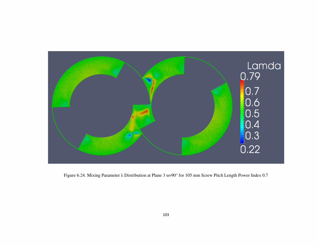
103
Figure 6.24. Mixing Parameter λ Distribution at Plane 3 α=90° for 105 mm Screw Pitch Length Power Index 0.7
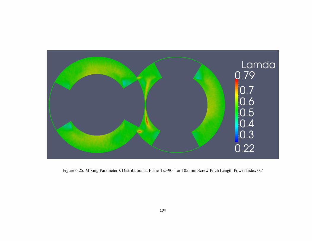
104
Figure 6.25. Mixing Parameter λ Distribution at Plane 4 α=90° for 105 mm Screw Pitch Length Power Index 0.7
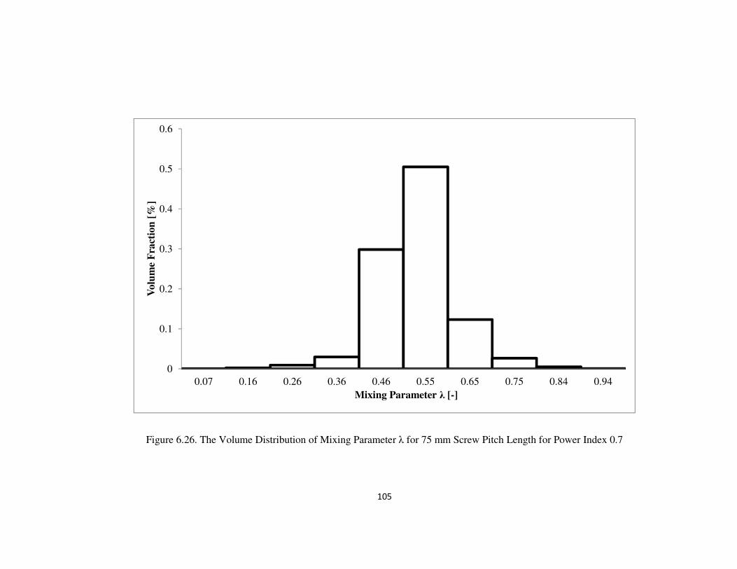
105
Figure 6.26. The Volume Distribution of Mixing Parameter λ for 75 mm Screw Pitch Length for Power Index 0.7
0
0.1
0.2
0.3
0.4
0.5
0.6
0.07 0.16 0.26 0.36 0.46 0.55 0.65 0.75 0.84 0.94
Vo
lum
e F
ract
ion
[%
]
Mixing Parameter λ [-]
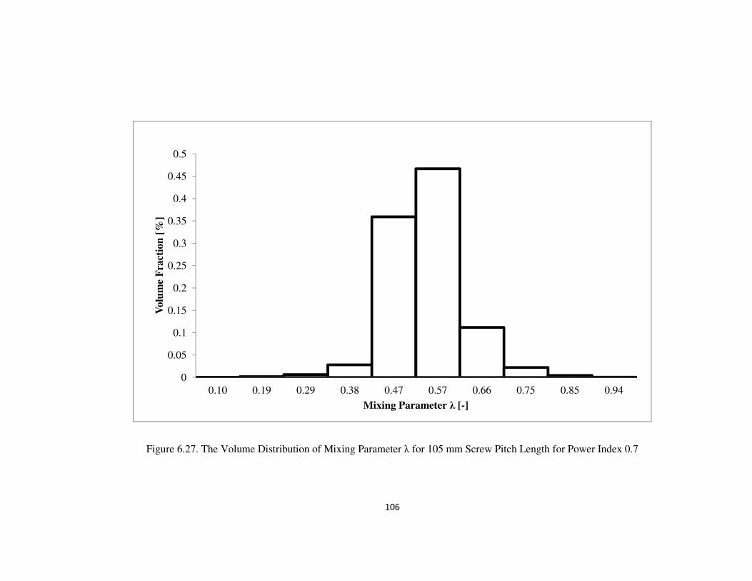
106
Figure 6.27. The Volume Distribution of Mixing Parameter λ for 105 mm Screw Pitch Length for Power Index 0.7
0
0.05
0.1
0.15
0.2
0.25
0.3
0.35
0.4
0.45
0.5
0.10 0.19 0.29 0.38 0.47 0.57 0.66 0.75 0.85 0.94
Vo
lum
e F
ract
ion
[%
]
Mixing Parameter λ [-]
107
Figure 6.28. The Volume Distribution of Mixing Parameter λ for 75 mm Screw Pitch Length for Power Index 0.3
0
0.1
0.2
0.3
0.4
0.5
0.6
0.07 0.16 0.26 0.36 0.46 0.55 0.65 0.75 0.84 0.94
Vo
lum
e F
ract
ion
[%
]
Mixing Parameter λ [-]
108
Figure 6.29. The Volume Distribution of Mixing Parameter λ for 105 mm Screw Pitch Length for Power Index 0.3
0
0.1
0.2
0.3
0.4
0.5
0.6
0.07 0.17 0.27 0.36 0.46 0.56 0.65 0.75 0.85 0.94
Vo
lum
e F
ract
ion
[%
]
Mixing Parameter λ [-]
109
Figure 6.30. The Average Mixing Parameter λ for Various Screw Speed and Screw Pitch Length Power Index 0.7
0.535
0.54
0.545
0.55
0.555
0.56
0 20 40 60 80 100 120
Mix
ing
Pa
ram
eter
λ
[-]
Screw Speed [rpm]
75mm
90mm
105mm
135mm
110
Figure 6.31. The Average Mixing Parameter λ for Various Screw Speed and Screw Pitch Length Power Index 0.3
0.534
0.536
0.538
0.54
0.542
0.544
0.546
0.548
0.55
0 20 40 60 80 100 120
Mix
ing
Pa
ram
eter
λ[-
]
Screw Speed [rpm]
75 mm
90 mm
105mm
135mm
111
Chapter Seven
COMPARASION OF SIMPLE FLOW MODEL AND COMPUTER
SIMULATION
7.1. Introduction
In this chapter, simple flow model, which is explored in Chapter 3, is
compared with computer simulation, covered in Chapter 6, in terms of flow
behaviour. Different screw lengths, flight width-to-channel width ratios and screw
speeds are compared for Newtonian fluid since simple flow model is only available
for Newtonian fluids.
7.2. Comparison of the Effect of the Screw Pitch Length
Screw Pitch lengths of 75 mm, 90 mm, 105 mm and 135 mm were used for
both simple flow model and computer simulation. Figure 7.1 indicates that both
simple flow model and computer simulation increase gradually with increasing screw
pitch length. Furthermore, increasing behaviour of mass flow rate decreases after 105
mm screw pitch length for both numerical and analytical solutions. Simple flow model
and computer simulation also provide similar results for mass flow rate.
7.3. Comparison of the Effect of Flight Width-to-channel Width Ratio
The ratios of flight width-to-channel width of 0.35, 0.5, 0.636 and 0.875 were
used.Figure 7.2 shows that mass flow rate decreases gradually with increasing the
flight width-to-channel width ratio. It is obvious in Figure 7.2 that computer
simulation and simple flow model provide very close mass flow rate results.
112
7.4. Comparison of the Effect of Screw Speeds
Screw speeds of 30, 60 and 120 rpm were investigated for both computer
simulation and simple flow model. It can be seen in Figures 7.3 and 7.4 that mass flow
rate increases proportionally with increasing screw speeds. Moreover, figures 7.3 and
7.4 indicate that numerical results match with simple flow model in the sense of mass
flow rate.
113
Figure 7.1. Comparison of the Effect of Screw Pitch Length for Computer Simulation and Simple Flow Model
200
220
240
260
280
300
320
340
360
380
75 90 105 120 135
Flo
w R
ate
[k
g/h
]
Screw Pitch Length[mm]
Computer
Simulation
Simple Flow
Model
114
Figure 7.2. Comparison of the Effect of the Flight Width-to-channel Width Ratio
for Computer Simulation and Simple Flow Model
200
220
240
260
280
300
320
340
360
380
0.2 0.4 0.6 0.8 1
Flo
w R
ate
[k
g/h
]
Flight Width/Channel Width[-]
Computer
Simulation
Simple Flow
Model
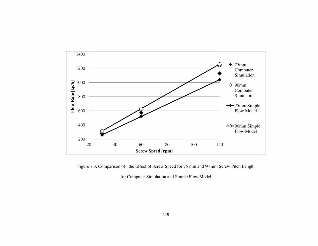
115
Figure 7.3. Comparison of the Effect of Screw Speed for 75 mm and 90 mm Screw Pitch Length
for Computer Simulation and Simple Flow Model
200
400
600
800
1000
1200
1400
20 40 60 80 100 120
Flo
w R
ate
[k
g/h
]
Screw Speed [rpm]
75mm
Computer
Simulation
90mm
Computer
Simulation
75mm Simple
Flow Model
90mm Simple
Flow Model
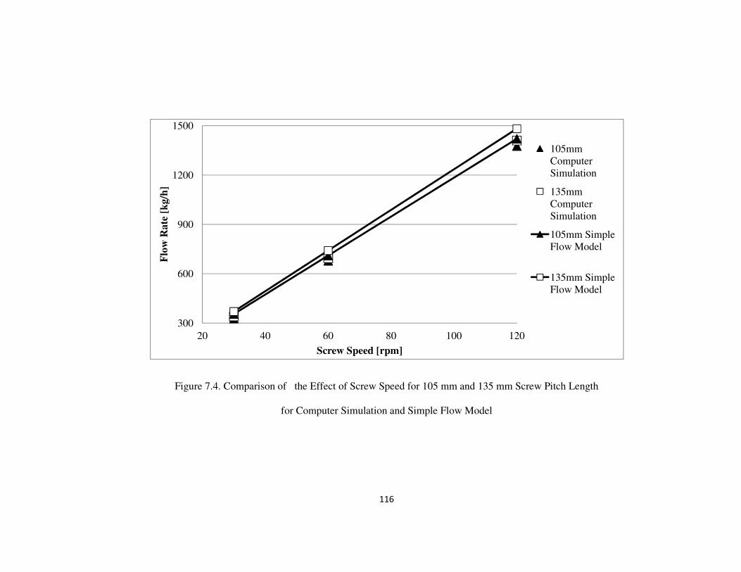
116
Figure 7.4. Comparison of the Effect of Screw Speed for 105 mm and 135 mm Screw Pitch Length
for Computer Simulation and Simple Flow Model
300
600
900
1200
1500
20 40 60 80 100 120
Flo
w R
ate
[k
g/h
]
Screw Speed [rpm]
105mm
Computer
Simulation
135mm
Computer
Simulation
105mm Simple
Flow Model
135mm Simple
Flow Model
117
Chapter Eight
CONCLUSION AND FUTURE WORK
8.1. Conclusion
The flow fields in the conveying section of the ICRTSE were obtained by
using OpenFOAM®, a computational fluid dynamic package, based on the
finite elements method. The problem of the time dependent moving
boundaries was examined by selecting a number of sequential geometries to
present a complete cycle. A good match was found between a simple
analytical model and the computer simulation for the Newtonian flow
condition, validating the simulation results in terms of pumping behaviour. For
simple analysis, this analytical model appears a sufficient tool to start the
design of the ICRTSE without necessitating the costly time to perform
computer simulations. The computer simulation are however necessary for
better understanding of the shear stress, shear rate and mixing etc. Design
decision can be made to reduce pumping efficiency or shear stress level for
shear sensitive material by using present model. The effect of different screw
pitch lengths, flight width to channel width ratios, screw speeds and power
indexes were investigated for pumping capacity and dispersive mixing
behaviour of ICRTSE. Screw pitch length and ratio of flight width to channel
width depend on each other geometrically, but it was decided to present the
results for both parameters because it is useful for screw design purposes.
118
From the computer simulations, it was noticed that shear thinning
behaviour of the fluid affects the pumping efficiency negatively. Secondly,
pumping efficiency decreases with increasing screw pitch length. In addition,
pumping efficiency goes up with increasing the ratio of flight width-to-
channel width. Finally, screw speed almost does not affect the pumping
efficiency at all.
Shear stress distribution was used to understand the dispersive mixing
behaviour of ICRTSE. The average shear stress decreases gradually with
increasing screw pitch length. Also, average shear stress is affected positively
from the ratio of flight width-to-channel width. Average shear stress increase
proportionally with increasing screw speed.
Dispersive mixing parameter lamda, λ, which quantifies the shear and
elongational flow, was used to understand the mixing efficiency of different
screw geometries and processing parameters. It is observed that the flow
inside conveying element of ICRTSE is dominated by shear flow. The mixing
parameter λ showed little variation by changing screw pitch length, ratio of
flight width-to-channel width, screw speed or power indexes.

119
8.2. Recommendations
• The simulation of complete sections of the ICRTSE involving
combination of mixing element and conveying element can be useful
for better understanding.
• A better model would require a transient solver, temperature effects,
distributive mixing and dispersive mixing for complete understanding
of ICRTSE.
120
REFERENCES
Alsteens, B., Legat, V., Avalosse, T., Int. Polym. Proc., XIX, 207-217, (2004).
Bravo, V.L., Hrymak, A.N., Wright, J.D., Polym. Eng. Sci., 40, 2, 525-541,
(2000).
Bravo, V.L., Finite Element Simulation of Flow in Twin screw Extruder
Mixing Elements, PhD Thesis, McMaster University, (1998).
Cheremisinoff, N.P., Polymer Mixing and Extrusion Technology, Marcel
Dekker Inc. (1987).
Doboczky, Z., Plast. Verarb., 16, 395 (19652).
Doboczky, Z., Plast. Verarb., 16, 57 (19651).
Dowson, D., Taylor, C. M., Ann. Rev. Fluid Mech., 11, 35-66 (1979).
Eggen, S.S., Syre, A., Homogenizing Multimodal Polymer, European Patent
EP1483311A1, (2004).
Fitzpatrick, H., Simulation and Characterization of Flow inside Twin Screw
Extruders, PhD Thesis, Howard University, (2009).
Gonzales-Avila, S.R., Klaseboer, E., Khoo, B.C., Ohl, C., J. Fluid Mech., 241-
260 (2011).
Gotsis, A.D., Ji, Z., Kalyon, D.M., Technical Papers SPE ANTEC, 139-142,
(1990).
121
Gupta, M., Vivek, R., Kuehn, R., Technical Papers SPE ANTEC, 2350-2355,
(2009).
Hong, M. H., White J. L., I., Int. Polym. Proc., XIII, 342-346, (1998).
Janssen, L. P. B. M., Twin Screw Extrusion, Elsevier, Amsterdam (1978).
Janssen, L.P.B.M., Mulders, L.P.H.R.M., Smith, J.M., Plastics and Polymers,
43, 93, (1975).
Jiang, Q., Modeling Flow, Melting, Solid Conveying and Global Behaviour in
Intermeshing Counter Rotating Twin Screw Extruders, PhD Thesis, University
of Akron, (2008).
Jiang, Q., Wilczynski, K., White, J.L., Technical Papers SPE ANTEC, 491-
496, (2007).
Juretic, F., Error Analysis in Finite Volume CFD, PhD Thesis, Imperial
College, (2004).
Ilinca F., Hetu J. -H., I., Int. Polym. Proc., XXV, 275-286, (2010).
Ilinca F., Hetu J. -H., I., Int. Polym. Proc., XXVII, 111-120, (2012).
Ishikawa, T., Kihara, S.I., Funatsu, K., Polym. Eng. Sci., 40, 2, 357-364,
(2000).
Kajiwara, T., Nagashima, Y., Nakano, Y., Funatsu, K., Polym. Eng. Sci., 36,
16, 2142-2152, (1996).
122
Klenk, K. P., Plast. Verarb., 17, IV/1-IV/9 (1966).
Klenk, K. P., Plast. Verarb., 22, 33 (1971).
Lawal, A., Railkar, S., Kalyon D. M., Technical Papers SPE ANTEC, (1999).
Lee, C. C., Castro J. M., Model Simplification, in Chapter 3 from Charles
Tucker III, Computer Modelling for Polymer Processing, Hanser (1989).
Li, T., Analysis of Mixing Efficiency in Continuous Polymer Processing
Equipment, PhD Thesis, Case Western Reserve University, (1995).
Li, T., Manas-Zloczower. I., Polym. Eng. Sci., 34, 7, 551-558, (1994).
Ma, X., Shi, F., Geng, X., Technical Papers SPE ANTEC, 3288-3292, (2004).
Manas-Zloczower, I. And Feke, D.L., Int. Polym. Proc., II, 185-190, (1988).
Manas-Zloczower, I. And Feke, D.L., Int. Polym. Proc., IV, 3-8, (1989).
Menges, G., Klenk, K. P., Plast. Verarb., 17, 791 (1966).
OpenFOAM, User’s Guide, Version 2.2.0, The OpenFOAM Foundation,
(2013).
Ortiz-Rodriquez, E., Tzoganakis, C., Technical Papers SPE ANTEC, 171-175,
(2009).
Ortiz-Rodriquez, E., Numerical Simulations of Reactive Extrusion in Twin
Screw Extrusion, PhD Thesis, University of Waterloo, (2009).
123
Potriefke, G., Int. Polym. Proc., XXI, 61-72, (2007).
Radl, S., Tritthart, T., Khinast, J.G., Chem. Eng. Sci., 65, 1976-1988, (2010).
Sakai, T., Hashimoto, N., Kobayashi, N., Technical Papers SPE ANTEC, 146-
151, (1987).
Schenkel, G., Kunststoffe Extrudertechnik, Hanser Verlag, Munich (1963).
Schenkel, G., Plastics Extrusion Technology and Theory, Iliffe Books Ltd.,
London, (1966).
Sebastian, D.H., Rakos, R.,Technical Papers, SPE ANTEC, 135-138 (1990).
Shah, A., Gupta, M., Technical Papers SPE ANTEC, 443-447 (2004).
Shon, K., Chang, D., White, J.L., Int. Polym. Proc., XIV, 44-50, (1999).
Sobhani, H., Nouri, M. R., Ghoreishy, M. H. R., Iran. Polym. J., 19, 143-154,
(2010).
Speur, J. A., Mavridis, H., Vlachopoulos, J., Janssen, L.P.B.M., Advances in
Polymer Technology, 7, 1, 39-48, (1987).
Szydlowski, W., Brzoskowski, R., White, J.L., Int. Polym. Proc., 1, 207-214,
(1987).
Valette, R., Coupez, T., David, C., Vergnes, B., Int. Polym. Proc., XXIV, 141-
147, (2009).
124
Yang, H.-H., Flow Field Analysis of Batch and Continuous Mixing
Equipment, PhD Thesis, Case Western Reserve University, (1993).
Yang, H. H., Manas-Zloczower, I., Int. Polym. Proc., VII, 195-203, (1992).
Yao, C. -H., Manas-Zloczower, I., Int. Polym. Proc., XII, 92-103, (1997).
Wang, C., Manas-Zloczower. I., Polym. Eng. Sci., 34, 15, 1224-1230, (1994).
White, J. L., Twin Screw Extrusion: Technology and Principles, Hanser, NY
(1990).
Wolf, D., Holin, N., White, D.H., Polym. Eng. Sci., 26, 9, 640-646, (1986).