modelling of energy consumption for algae photo
TRANSCRIPT
Page I
Thesis Systems and Control
Systems and Control Group
Modelling of energy
consumption for algae photo
bioreactors in various scenarios
Ing. R.S.K. Girdhari
Supervisors: Ir. P.M. Slegers Dr. Ir. A.J. B. van Boxtel
19 December 2011

Page II
Page III
Modelling of energy
consumption for algae photo
bioreactors in various scenarios
Name course : Thesis project Systems and Control Number : SCO-80436 Study load : 36 ects Date : 19 December 2011 Student : Ing. R.S.K. Girdhari Registration number : 87-07-09-265-010 Study programme : MBT (Biotechnology) Supervisor(s) : Ir. P.M. Slegers and Dr. Ir. A.J.B. van Boxtel Examiners : Dr. Ir. K.J. Keesman Group : Systems and Control Group Address : Bornse Weilanden 9 6708 WG Wageningen the Netherlands Tel: +31 (317) 48 21 24 Fax: +31 (317) 48 49 57

Page IV
Page V
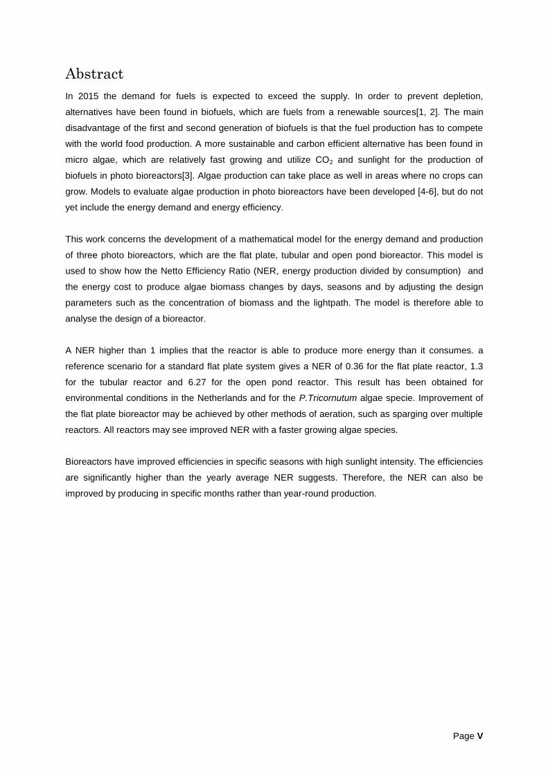
Abstract
In 2015 the demand for fuels is expected to exceed the supply. In order to prevent depletion,
alternatives have been found in biofuels, which are fuels from a renewable sources[1, 2]. The main
disadvantage of the first and second generation of biofuels is that the fuel production has to compete
with the world food production. A more sustainable and carbon efficient alternative has been found in
micro algae, which are relatively fast growing and utilize CO2 and sunlight for the production of
biofuels in photo bioreactors[3]. Algae production can take place as well in areas where no crops can
grow. Models to evaluate algae production in photo bioreactors have been developed [4-6], but do not
yet include the energy demand and energy efficiency.
This work concerns the development of a mathematical model for the energy demand and production
of three photo bioreactors, which are the flat plate, tubular and open pond bioreactor. This model is
used to show how the Netto Efficiency Ratio (NER, energy production divided by consumption) and
the energy cost to produce algae biomass changes by days, seasons and by adjusting the design
parameters such as the concentration of biomass and the lightpath. The model is therefore able to
analyse the design of a bioreactor.
A NER higher than 1 implies that the reactor is able to produce more energy than it consumes. a
reference scenario for a standard flat plate system gives a NER of 0.36 for the flat plate reactor, 1.3
for the tubular reactor and 6.27 for the open pond reactor. This result has been obtained for
environmental conditions in the Netherlands and for the P.Tricornutum algae specie. Improvement of
the flat plate bioreactor may be achieved by other methods of aeration, such as sparging over multiple
reactors. All reactors may see improved NER with a faster growing algae species.
Bioreactors have improved efficiencies in specific seasons with high sunlight intensity. The efficiencies
are significantly higher than the yearly average NER suggests. Therefore, the NER can also be
improved by producing in specific months rather than year-round production.

Page VI
Page VII
Table of Contents
Abstract.................................................................................................................................................... V
1. Introduction .......................................................................................................................................... 2
2. The model ............................................................................................................................................ 4
2.1 Biological processes and environmental exchange ....................................................................... 5
2.1.1 Cultivation of algae .................................................................................................................. 5
2.1.2 Sunlight intensity ..................................................................................................................... 6
2.1.3 Radiation loss .......................................................................................................................... 6
2.1.4 Convection .............................................................................................................................. 7
2.2 Physical processes flat plate reactor ............................................................................................. 9
2.2.1 Inflow of fresh medium ............................................................................................................ 9
2.2.2 aeration ................................................................................................................................. 10
2.2.3 Temperature control .............................................................................................................. 10
2.3. Physical processes tubular reactor ............................................................................................. 12
2.3.1 Flow ....................................................................................................................................... 13
2.3.2. Degassing ............................................................................................................................ 13
2.3.3 determining the total energy requirement ............................................................................. 15
2.4 Physical processes pond reactor ................................................................................................. 15
2.4.1 Energy requirement of the paddle wheel and CO2 injection ................................................. 16
2.4.2 Energy requirements for the inflow and outflow .................................................................... 17
2.5 Reference scenarios .................................................................................................................... 18
2.5.1 Scenarios for the flat plate photobioreactor ......................................................................... 18
2.5.2 Scenarios for the tubular photobioreactor ............................................................................. 19
2.5.3 Scenarios for the pond reactor .............................................................................................. 19
3. Results ............................................................................................................................................... 20
3.2 Results flat panel photobioreactor ............................................................................................... 20
3.2 Results Tubular reactor................................................................................................................ 25
3.4 Results Open pond reactor .......................................................................................................... 32
4. Discussion ......................................................................................................................................... 38
5. Conclusion ......................................................................................................................................... 42
References ............................................................................................................................................ 44
Acknowledgements ............................................................................................................................... 46
Annex A: Constant factors ..................................................................................................................... 48
Annex B: Nomenclature ......................................................................................................................... 50

Page 1
Page 2
1. Introduction
In 2015 the demand for fuels is expected to exceed the supply[7], which will become a worldwide
concern. In order to prevent complete depletion, alternatives have been found in biofuels, which are
fuels from a renewable source[1, 2]. The main disadvantage of the first and second generation of
biofuels is that the fuel production has to compete with the world food production. A more sustainable
and carbon efficient alternative has been found in micro algae, which are relatively fast growing and
utilize CO2 and sunlight for the production of biofuels in a photo bioreactor [3].
The cultivation of algae on large scale happens in different production systems; an open system, such
as an open pond (raceway) or in closed systems, such as a flat panel reactor or a tubular reactor. The
main difference between the two systems is that an open system has a lower variable (biomass)
production cost, but a closed system has a higher yield. Wijffels et al[8]. expects that after
optimization of the closed photo bioreactor the production costs can become lower than in an open
photo bioreactor[8]. Algae biomass is further processed into biofuel after the cultivation.
The cultivation of algae has some challenges; next to the high costs of biomass production, a
sufficient amount of land is required to obtain enough sunlight for production. Only part of the sunlight
is used and therefore the reactor in the summer is heated up. On the other hand, in winter the ambient
temperature might not be sufficient enough to sustain the optimal growth conditions of the photo
bioreactor and needs to be heated.
The energy consumption of a photo bioreactor contributes significantly to the running costs of the
cultivation process. Lehr et al.[9] concludes that a high amount of supplied energy during cultivation is
one of the reasons that biodiesel from algae currently cannot compete with diesel production. Norsker
et al. [10] have investigated the economic outlook for photo bioreactor and concludes that costs
should be reduced by approximately 80-90% in order to make the process feasible. However, Cheng-
Wu et al [11] states that the energy cost is surmounted by labour costs for an industrial flat plate
reactor and therefore not significant.
In order to gain insight of how the energy balance of a photo bioreactor can be optimised a
mathematical model is required. It is important to realise the different constructions between the
different production systems. An open pond (raceway) system suffers from e.g. evaporation of water
from the pond whereas in a closed system this phenomena does not occur. There are already several
models for the prediction of production with respect to sunlight. In these models, the sunlight
penetration is calculated and the production is estimated by Lambert-Beer equations combined with
Geiders[12] cultivation model[4-6]. These models have laid the emphasis on the production of algae
biomass, so that the energy production can be estimated. These models have not yet considered the
energy balances involved for the reactors, such that the netto energy yield of a reactor cannot be fully
shown. Lehr et al [9] argues that the external energy input requirement for a tubular reactor is
Page 3
considerably large, such that a tubular reactor cannot be profitable for energy production. Energy
reducing should therefore be employed before the configuration can be used, but no model exists at
this point, to show the change of energy yield, per change in a reactor.
Norsker et al[10], has depicted the most energy cost intensive processes for the different reactor types
from general engineering rules. These are the sparging for the flat plate reactor, degassing for the
tubular reactor and the paddle wheel for the raceway pond[10]. Next to this the cultivation systems are
dependent on other factors, such as the environmental conditions and biological demands of the
algae. Although these may not require the largest amount of energy, it is unclear how much they
contribute to the total energy demand. Further research is needed to gain more insight in ways to
reduce the amount of energy required to produce algae for the production of biodiesel.
This mathematical model is used to evaluate several scenarios for comparison. These scenarios are
developed for the Netherlands. For this purpose the model for the energy balances is developed and
linked to the production and cultivation models of Slegers, van Beveren and Lösing[4-6]. With this
combination it is possible to evaluate the total energy requirements of a photobioreactor under
different conditions, such as the design parameters, algae concentration and so on. Various
environmental data, such as temperature, humidity and light intensity have been measured over 2009
in a 10 minute interval. The cultivation of algae has been modelled separately for the three different
configurations. The production values of such models are added as an external input for the
mathematical model. The goal of this model is to provide a method to show how the energy demand
and netto energy yield changes on an yearly average.
Page 4
2. The model
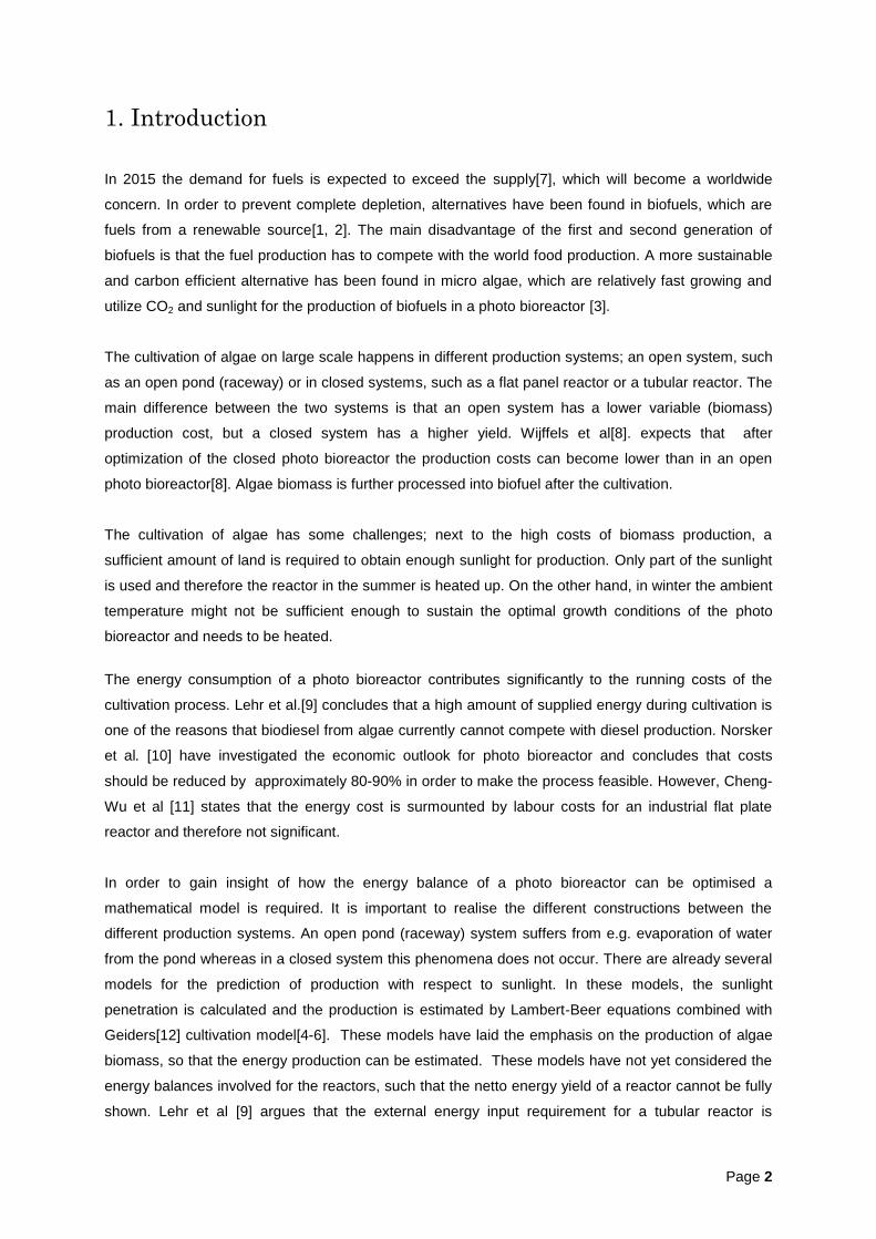
For algae cultivation open and closed photobioreactors are used (figure 1). In open photobioreactors
(open pond) the cultivation broth is in direct contact with the environment and exchange of heat and
water (vapour) occurs directly. The cultivation broth in closed photobioreactors is not in direct contact
with the open air and there is no water (vapour) exchange while heat exchange only occurs through
the reactor wall. Among the closed systems the flat plate and tubular systems have the most attention.
In this chapter the energy required for a photobioreactor is quantified. For an open pond it concerns
the paddle wheel and CO2 supply. Open systems are mostly not temperature controlled and therefore
the energy calculations to keep the system at a required temperature are not considered. For a closed
system the energy for CO2 supply, fluid recirculation, and the energy for controlling the temperature
are considered.
Figure 1: from left to right: tubular reactor, flat plate reactor and an open pond reactor
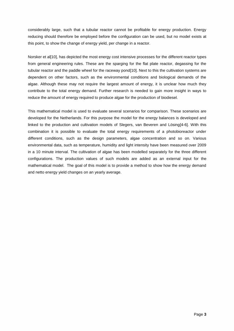
To calculate the energy demand for the system, three different categories of processes are
considered: Biological (growth of algae), exchange with the environment (e.g. radiation, sunlight) and
physical units for the required conditions (e.g. pumps). Their inner relation is depicted in figure 2.
Figure 2: the relation between the biological, environmental and physical processes
Whereas biological processes and environmental exchange show similarities , physical processes
differ for each configuration. The biological processes and environmental exchanges will be explained
in section 2.1 and physical processes in section 2.2.
Page 5
2.1 Biological processes and environmental exchange
The biological processes and environmental exchanges contribute to the thermal energy balance,
which results in temperature fluctuations in the reactor. A cooling/heating unit is used to keep the
temperature constant. The cooling/heating unit requests for electrical energy to provide the
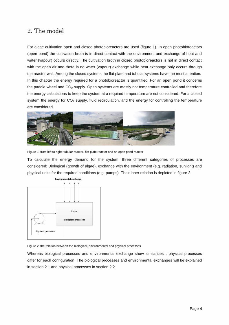
cooling/heating medium, together with other physical processes. A schematic overview of biological
processes and environmental exchange is given in figure 3.
Figure 3: biological processes and environmental exchange in a closed photobioreactor
The biological process of the reactor consists of the cultivation of algae, whereas the environmental
exchange consists of the intensity of the sun entering the reactor , radiation and convective energy
dissipation of the reactor.
2.1.1 Cultivation of algae
The cultivation of algae concerns growth and maintenance. Slegers[4] and van Beveren[6] have
extensively described the algae production and sunlight simulation of a flat plate and a tubular
photobioreactor respectively. The energy uptake of the algae, assuming the concentration in the
reactor remains constant, is described as,
(1)
Where is the energy requirement of the algae in [J s
-1], is the combustion energy of the
algae in [J kg-1
], is the production of the reactor in [kg s-1
], rmax is the maximum maintenance
coefficient in [s-1
], Cx is the concentration of the algae in [kg m-3
] and V is the volume in [m3].
The production term follows from the actual growth or algae outflow from the reactor, according to the
steady state mass balance,
(2)
(3)
Where is the growth rate of the algae in [s-1
] and is the outflow of the reactor [m3s
-1].
Constant factors such as the combustion energy are found in annex A.
Page 6
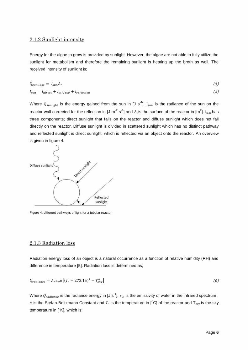
2.1.2 Sunlight intensity
Energy for the algae to grow is provided by sunlight. However, the algae are not able to fully utilize the
sunlight for metabolism and therefore the remaining sunlight is heating up the broth as well. The
received intensity of sunlight is;
(4)
(5)
Where is the energy gained from the sun in [J s
-1], is the radiance of the sun on the
reactor wall corrected for the reflection in [J m-2
s-1
] and is the surface of the reactor in [m2]. Isun has
three components; direct sunlight that falls on the reactor and diffuse sunlight which does not fall
directly on the reactor. Diffuse sunlight is divided in scattered sunlight which has no distinct pathway
and reflected sunlight is direct sunlight, which is reflected via an object onto the reactor. An overview
is given in figure 4.
Figure 4: different pathways of light for a tubular reactor
2.1.3 Radiation loss
Radiation energy loss of an object is a natural occurrence as a function of relative humidity (RH) and
difference in temperature [5]. Radiation loss is determined as;
[( )
] (6)
Where is the radiance energy in [J s-1
], is the emissivity of water in the infrared spectrum ,
is the Stefan-Boltzmann Constant and is the temperature in [oC] of the reactor and Tsky is the sky
temperature in [oK], which is;
Page 7
( ) [
( )]
(7)
Where Ta is the air temperature in [oC], Tdew is the dewpoint temperature and tsolar is the elapsed time
after midnight in [hr]. The air temperature is assumed to be equal to the ambient temperature as
collected in the same dataset of the sunlight. The dewpoint temperature is estimated from;
(
)
(
) (8)
Where ea is the water pressure of the air, which is calculated as;
(9)
The relative humidity (RH) has been measured in the same dataset as sunlight intensity. The
cloudiness of the air has not been taken into consideration as such data was not available. This may
have an effect on the radiation losses.
2.1.4 Convection
The ambient temperature has an influence on the reactor due to convection. Bird et al[13] gives a
resistance based approach to determine this fluctuation which is described as;
(for flat surfaces) (10)
( )
(for curved surfaces) (11)
Where Ta is the environmental temperature in [oC], r is the radius of the tube in [m] and h is the heat
transfer coefficient in [W m-2 o
C-1
]. The resistance is the path where the convection stream has to go
through between the liquid and air. This is shown as;
(for a flat surfaces) (12)
( )
(for curved surfaces) (13)
Where k [W m-1o
C-1
] is the heat conductivity of the material, L [m] is the thickness of the wall between
the broth and air, r1[m] is the outer surface radius and r2[m] is the inner surface radius. The heat
transfer coefficient h [W m-2o
C-1
] is calculated as following;
(14)
Page 8
where Nnu is the Nusselt, number and l as the specific length [m] which is defined as
( )
( ) for water and (15)
( )
( ) for air (16)
In a flat plate reactor and
l = 2r for a tubular reactor (17)
Where w is the width [m], z is the depth [m] and he is the height of the reactor [m].
The Nusselt number follows from the Prandtl number and the Reynolds number [14];
(for a flat plate reactor turbulent flow) (18)
(for a flat plate reactor laminar flow) (19)
(for a tubular reactor turbulent flow) (20)
(
)
(for a tubular reactor laminar flow) (21)
Where Npr and Nre are the Prandtl and Reynolds number respectively, which follows from,
(22)
(23)
Where μ is the kinematic viscosity in [Pa s]. For the broth the Reynolds number and Prandtl number
calculated found by using the properties of water, see table 1. For the environment the fluctuating
temperature and wind velocity have to be taken into account. The properties of air are found by using
empirical relations1 as a function of the ambient temperature, which are described as follows;
(24)
(25)
(26)
(27)
Where is the ambient temperature in [oC], is the density of air in [kg m
-3] and is the specific
heat of air in [J kg-1o
C-1
].
1 Derived from the engineering toolbox: http://www.engineeringtoolbox.com/air-properties-d_156.html
(accessed 13 December 2011)
Page 9
Table 1: properties of water
Property Value Unit
10-3
Pa s
1000 Kg m-3
4180 J Kg-1 o
C-1
0.58 W m-1o
C-1
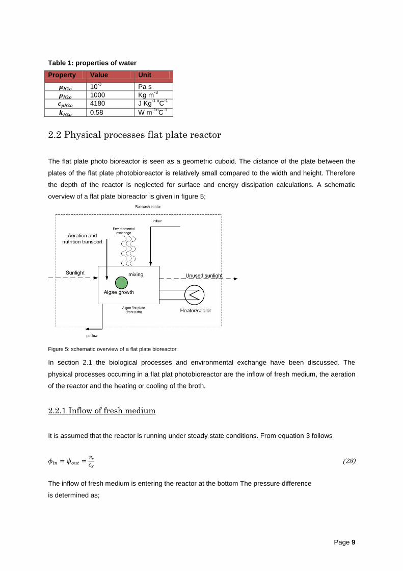
2.2 Physical processes flat plate reactor
The flat plate photo bioreactor is seen as a geometric cuboid. The distance of the plate between the
plates of the flat plate photobioreactor is relatively small compared to the width and height. Therefore
the depth of the reactor is neglected for surface and energy dissipation calculations. A schematic
overview of a flat plate bioreactor is given in figure 5;
Figure 5: schematic overview of a flat plate bioreactor
In section 2.1 the biological processes and environmental exchange have been discussed. The
physical processes occurring in a flat plat photobioreactor are the inflow of fresh medium, the aeration
of the reactor and the heating or cooling of the broth.
2.2.1 Inflow of fresh medium
It is assumed that the reactor is running under steady state conditions. From equation 3 follows
(28)
The inflow of fresh medium is entering the reactor at the bottom The pressure difference
is determined as;
Page 10
(29)
Where P is the pressure in [pa]. The energy required to overcome the pressure is equal to;
(30)
A method to determine the energy equivalent cost in ct€ per kg biomass is;
(31)
Where is the cost for the inflow in [ct€ kg
-1], is the pump efficiency and is the cost of
Kwh in [ct€ kwh-1
]. The cost is a rate of consumption over the timespan for the energy requirement and
biomass production.
2.2.2 aeration
The aeration is done by bubbling in microbubbles from the bottom of the reactor in order to create
enough mixing within the tank in such a way that no mechanical mixing is required. Norsker states that
the energy requirement of a cycloblower for a flat plate photobioreactor is
110 [m3 hr
-1 Kw
-1] and the inflow requirement of such reactor is equal to
1 [m3 min
-1 m
-3(volume)]. The air flow for a specific flat plate photobioreactor is equal to;
(32)
Where is the aeration requirement in [m
3 hr
-1], is the aeration demand as proposed
by Norsker, is the volume of the reactor and is a correction factor(minutes to hour). The
energy requirement is then determined as;
(33)
Where is the energy requirement of the specific reactor in [Kw], is the energy demand
as proposed by Norsker and is a conversion factor from (hour to seconds). Finally the cost per
kg biomass is determined similar to equation 31;
(34)
2.2.3 Temperature control
The temperature of the broth remains constant to obtain optimal conditions for algae growth. The
shortage or excess of heat is determined as;
Page 11
(35)
The right-hand side is the sum of the biological processes and environmental exchanges, as explained
in section 2.1. If Qreactor is negative the reactor needs to heat up and vice versa if Qreactor is positive it
needs to cool down such that;
(36)
Cooling of the reactor happens by an evaporative cooling unit. It is assumed that the conditions are
good enough to evaporate the water without constraints. This gives an evaporation flow of;
(37)
Where is the amount of energy one unit of water can evaporate [kJ Kg]. Heating up the reactor is
done by a heat exchanger such that;
( ) (38)
Where the temperature of the heater, Theater, is always higher than the temperature of the reactor.
Rearrangement yields the water flow required to heat up the reactor. Lumping the cooling and heating
flows together gives the temperature fluctuation flow, . The energy requirements are determined
via the extended Bernoulli equation, which is
( (
) (
)
) (39)
Where [J s
-1] is the energy requirement, Nfan is the fanning friction factor, Ltube [m] is the length of
the tubing, Dtube [m] is the diameter of the tubing, [m s-1
] is the superficial liquid velocity and g is
the gravitational constant in [m s-2
]. The superficial liquid velocity is determined as;
(40)
(41)
Where At is the cross sectional area of the cooling/heating tube. The fanning friction factor is
dependent of the Reynolds number, which is determined as;
√
(for laminar flows) (42)
(for turbulent flows) (43)
Page 12
Equation 43 is known as the Blasius equation. The cost for cooling and heating is determined similar
to equation 31,
(44)
Where is the pump efficiency. The total rate of consumption for a flat plate reactor is determined as
(45)
2.3. Physical processes tubular reactor
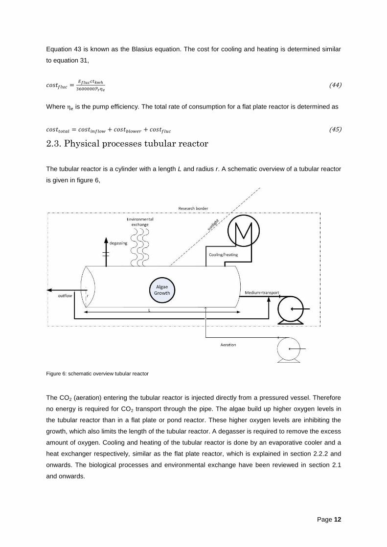
The tubular reactor is a cylinder with a length L and radius r. A schematic overview of a tubular reactor
is given in figure 6,
Figure 6: schematic overview tubular reactor
The CO2 (aeration) entering the tubular reactor is injected directly from a pressured vessel. Therefore
no energy is required for CO2 transport through the pipe. The algae build up higher oxygen levels in
the tubular reactor than in a flat plate or pond reactor. These higher oxygen levels are inhibiting the
growth, which also limits the length of the tubular reactor. A degasser is required to remove the excess
amount of oxygen. Cooling and heating of the tubular reactor is done by an evaporative cooler and a
heat exchanger respectively, similar as the flat plate reactor, which is explained in section 2.2.2 and
onwards. The biological processes and environmental exchange have been reviewed in section 2.1
and onwards.
Page 13
2.3.1 Flow
The flow of the reactor is based on the Reynolds number. For minimal turbulent flow around spherical
objects the flow requires a Reynolds number of at least 1000. The superficial liquid velocity follows
from rearranging equation 22,
( ) (46)
The flow inside the tube is then determined as,
(47)
Where At is the cross sectional area of the tube similar to equation 41. Friction occurs in the pipe due
to recirculation. Two elbow pipes and two T-split piping are used for recirculation in the model. The
energy required for the flow in the tube is determined by the extended Bernoulli equation including
friction of the pipe for recirculation ,
( (
)
( ) )
(48)
Where Ltube [m] is in straight part equivalent in meter and 1.8 and 1.2 are friction factors for the elbow
pipe and T-split tubing respectively. The costs can be calculated by an equation similar to equation 31
(49)
2.3.2. Degassing
Oxygen can leave a flat plate system easier than a tubular reactor. These higher levels of oxygen in
the tubular reactor are inhibiting the algae growth and eventually will decrease the production. A
degassing unit is required to remove the excess amount of oxygen. A schematic overview of the
degasser is given in figure 7.
Under steady state conditions the equilibrium of the degasser is given as,
( ) ( ) (50)
Where is the gas flow in [m3s
-1], is the amount of oxygen in air in [mol m
-3] for the inflow and
outflow of air in the degassing unit, is the broth flow and is the oxygen concentration in the
broth entering and exiting the degasser. Equation 50 is based on certain assumptions, firstly the
oxygen concentration in the liquid leaving the degasser (xo2, out) is fixed. This is set as 0.3 [mol m-3
][6],
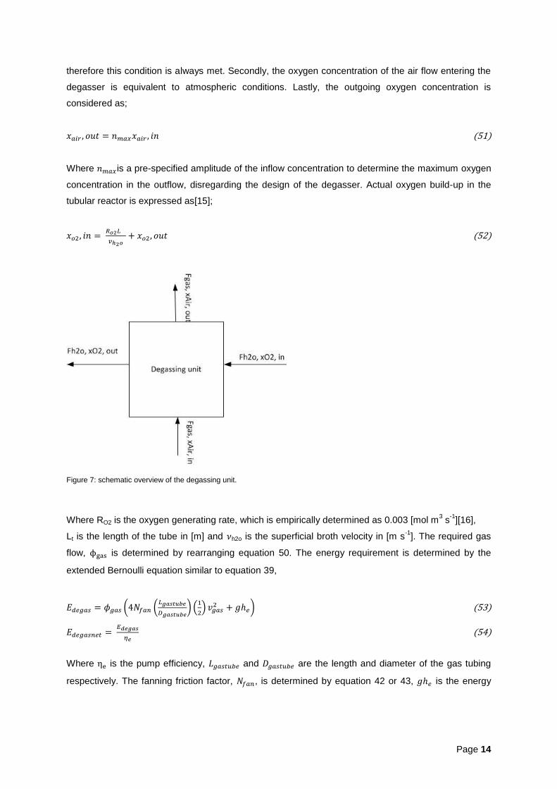
Page 14
therefore this condition is always met. Secondly, the oxygen concentration of the air flow entering the
degasser is equivalent to atmospheric conditions. Lastly, the outgoing oxygen concentration is
considered as;
(51)
Where is a pre-specified amplitude of the inflow concentration to determine the maximum oxygen
concentration in the outflow, disregarding the design of the degasser. Actual oxygen build-up in the
tubular reactor is expressed as[15];
(52)
Figure 7: schematic overview of the degassing unit.
Where RO2 is the oxygen generating rate, which is empirically determined as 0.003 [mol m3 s
-1][16],
Lt is the length of the tube in [m] and h2o is the superficial broth velocity in [m s-1
]. The required gas
flow, is determined by rearranging equation 50. The energy requirement is determined by the
extended Bernoulli equation similar to equation 39,
( (
) (
)
) (53)
(54)
Where is the pump efficiency, and are the length and diameter of the gas tubing
respectively. The fanning friction factor, , is determined by equation 42 or 43, is the energy
Page 15
requirement to overcome the water pressure in the degasser and is the superficial gas velocity of
the gas [m s-1
], which is determined as
(55)
The cost requirement is analogue to equation 44,
(56)
2.3.3 determining the total energy requirement
The cooling and heating requirement are determined by equation 44 which is,
(57)
Together with equation 49 and 56 the total rate of consumption is determined as;
(58)
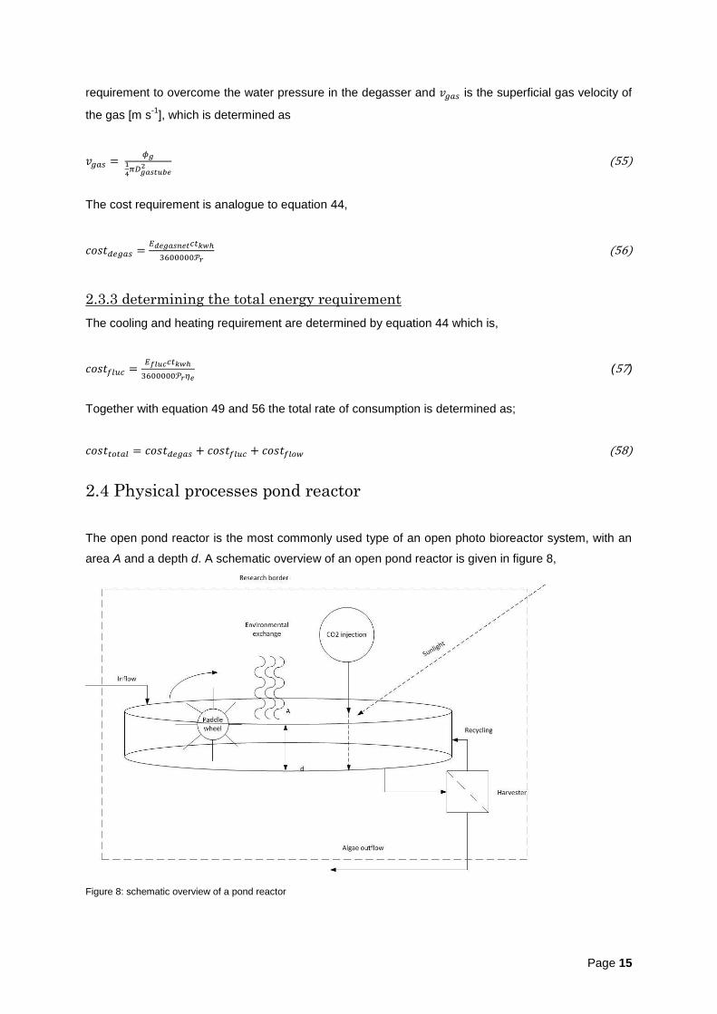
2.4 Physical processes pond reactor
The open pond reactor is the most commonly used type of an open photo bioreactor system, with an
area A and a depth d. A schematic overview of an open pond reactor is given in figure 8,
Figure 8: schematic overview of a pond reactor
Page 16
The open pond system has two distinguished geometrical shapes. It is either a man-made or a natural
lake or a raceway system. To compensate for the production outflow (equation 3) and the evaporation,
an inflow pump is required. After the cultivation step (both open and closed systems), a harvesting
step occurs. The algae concentration in pond reactors is significantly lower than in closed systems, to
compensate for this in analysis, a harvesting step is included in the pond reactor to compensate the
cost requirement for more insight in comparison with the closed system. Finally a paddle wheel is
required for stirring and degassing. CO2 has to be injected to compensate for the CO2 requirements.
The water entering the open pond due disturbances in the weather (rain, snow, etc.) has not been
considered as such data was not available.
2.4.1 Energy requirement of the paddle wheel and CO2 injection
The paddle wheel roughly uses2 5000 W ha
-1 or 0.5 W m
-2. The energy cost to run the paddle wheel is
therefore,
(59)
Where Apond is the surface area of the pond reactor [m2]. The CO2 requirement is linked to the
stoichiometric requirement of the algae, as the aeration is not required for the pond reactor. The
stoichiometric growth equation of P. Tricornutum is
(60)
Where is the representation of the algae. This implies that 1 mol of CO2 is
used for 1 mol of algae.
The CO2 inflow is determined as;
(61)
Where ysur is a surplus factor of CO2 and is the density in [kg m
-3]. The energy requirement for the
CO2 is then determined by the extended Bernoulli equation similar to equation 39;
( (
) (
)
) (62)
The Fanning friction factor, Nfan, is determined by equation 42 or 43, and are the
length and diameter of the supply tube of CO2 respectively. is the term to overcome the water
pressure of the reactor. is the superficial gas velocity, which is determined similar as equation 55.
2Personal communications Norsker June 2011
Page 17
The cost equation is applied, which is analogue to equation 46;
(63)
2.4.2 Energy requirements for the inflow and outflow
The inflow of the reactor is determined by the production and evaporative losses such that,
(64)
Where is the evaporation energy loss and is the evaporation energy of water in [J m
-3]
Due to the harvester the inflow is reduced as the outflow is concentrated. The removed water from the
harvester is returned to the pond, which will decrease the inflow. The reduction ratio is determined as
(65)
Which gives the new inflow as
(66)
The evaporation heat loss is determined by [5]
( ) (67)
Where is the evaporative transfer function, is the saturated water pressure and is the
saturated air pressure, which are determined as[5],
(68)
(9)
(69)
Where Ta and are the ambient and water temperature respectively and is the wind velocity
in [m s-1
]. The energy requirement for the inflow is determined by the Bernoulli equation similar to
equation 62
( (
)(
) )
(70)
Where the superficial inflow velocity is determined as equation 55.
Harvesting the algae with the purpose of concentrating the algae outflow stream is done by a
separator, which costs 1.1 KwH m-3
[10]. It is assumed that this energy requirement includes
recirculation of the excluded water as well. Therefore the cost for the inflow and outflow is determined
as,
( )
(71)
(72)
The total rate of consumption for the pond reactor then
(73)
Page 18
2.5 Reference scenarios
In order to compare the energy consumption of the three models with each other, the rate of
consumption of energy per kilogram dry weight of algae is determined. A harvesting step is
implemented for the open pond reactor, to compensate for the low biomass concentration in
comparison with the closed systems. Every ten minutes a weather data point from 2009 was
taken[17], to provide the environmental conditions of the model. The data concerned the biomass
production, sunlight, wind velocity, relative humidity and the ambient temperature. The models are
compared on their efficiency, which is shown as their Netto Energy Ratio (NER). The NER is
determined as,
(74)
Where is the combustion energy of algae and is the total energy demand of the reactor.
When the NER is smaller than 1, the produced energy from the algae is not enough to sustain the
variable energy cost and is therefore not efficient. The simulations run in MatLAB (version 2011A).
The program is administered at the system and control group of Wageningen University and
Research.
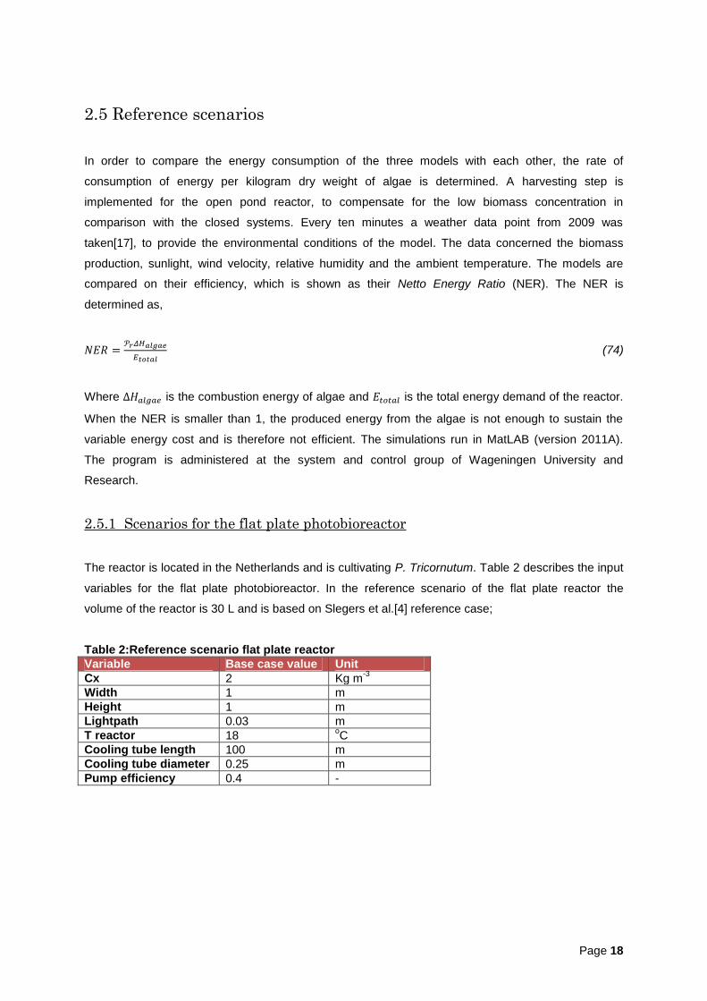
2.5.1 Scenarios for the flat plate photobioreactor
The reactor is located in the Netherlands and is cultivating P. Tricornutum. Table 2 describes the input
variables for the flat plate photobioreactor. In the reference scenario of the flat plate reactor the
volume of the reactor is 30 L and is based on Slegers et al.[4] reference case;
Table 2:Reference scenario flat plate reactor
Variable Base case value Unit
Cx 2 Kg m-3
Width 1 m
Height 1 m
Lightpath 0.03 m
T reactor 18 oC
Cooling tube length 100 m
Cooling tube diameter 0.25 m
Pump efficiency 0.4 -
Page 19
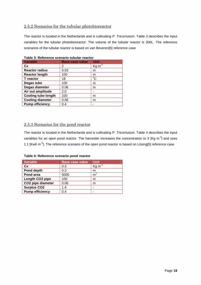
2.5.2 Scenarios for the tubular photobioreactor
The reactor is located in the Netherlands and is cultivating P. Tricornutum. Table 3 describes the input
variables for the tubular photobioreactor. The volume of the tubular reactor is 300L. The reference
scenarios of the tubular reactor is based on van Beveren[6] reference case
Table 3: Reference scenario tubular reactor
Variable Base case value Unit
Cx 2 Kg m-3
Reactor radius 0.03 m
Reactor length 100 m
T reactor 18 oC
Degas tube 100 m
Degas diameter 0.06 m
Air out amplitude 2.0 -
Cooling tube length 100 m
Cooling diameter 0.06 m
Pump efficiency 0.4 -
2.5.3 Scenarios for the pond reactor The reactor is located in the Netherlands and is cultivating P. Tricornutum. Table 4 describes the input
variables for an open pond reactor. The harvester increases the concentration to 3 [Kg m-3
] and uses
1.1 [Kwh m-3
]. The reference scenario of the open pond reactor is based on Lösing[5] reference case
Table 4: Reference scenario pond reactor
Variable Base case value Unit
Cx 0.3 Kg m-3
Pond depth 0.3 m
Pond area 5000 m2
Length CO2 pipe 100 m
CO2 pipe diameter 0.06 m
Surplus CO2 1.4 -
Pump efficiency 0.4 -

Page 20
3. Results
For the three systems the energy costs per kilogram biomass, the most energy cost intensive process
and the netto energy efficiency are calculated. The reference scenarios of section 2.5 have been used
to investigate the changes in the energy consumption when changing input variables. The investment
costs of the reactor have been disregarded.
3.1 Results flat panel photobioreactor
The production of the flat plate reactor varies with lightpath and the concentration as shown in figure
9[4]. The reactor has an certain optimum production depending on the concentration and lightpath,
which is around 11 [Kg panel-1
year-1
]. Increasing the concentration results in a decrease of
production, due to the algae biomass being too dense to receive enough light. In extreme cases, this
respiration may overrule the growth of the algae culture,
Figure 9: yearly production of biomass in a flat plate reactor with for different distances between the plates based on Slegers[4]
The energy costs for biomass production is independent of the production, but it is influenced by the
volume. The energy consumption linearly increases with the volume as shown in figure 10.
0 1 2 3 4 5 6 7 8 9 100
2
4
6
8
10
12
Cx [kg/m3]
avera
ge P
roduction [
Kg/(
panel *
year)
]
d = 0.01 [m]
d = 0.03 [m]
d = 0.05 [m]
Page 21
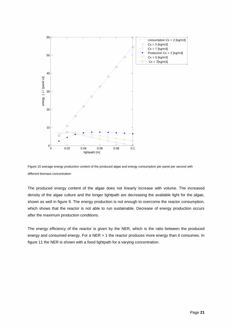
Figure 10 average energy production content of the produced algae and energy consumption per panel per second with
different biomass concentration
The produced energy content of the algae does not linearly increase with volume. The increased
density of the algae culture and the longer lightpath are decreasing the available light for the algae,
shown as well in figure 9. The energy production is not enough to overcome the reactor consumption,
which shows that the reactor is not able to run sustainable. Decrease of energy production occurs
after the maximum production conditions.
The energy efficiency of the reactor is given by the NER, which is the ratio between the produced
energy and consumed energy. For a NER > 1 the reactor produces more energy than it consumes. In
figure 11 the NER is shown with a fixed lightpath for a varying concentration.
0 0.02 0.04 0.06 0.08 0.10
10
20
30
40
50
60
lightpath [m]
energ
y
[ J /
(panel s)]
consumption Cx = 2 [kg/m3]
Cx = 5 [kg/m3]
Cx = 7 [kg/m3]
Production Cx = 2 [kg/m3]
Cx = 5 [kg/m3]
Cx = 7[kg/m3]
Page 22
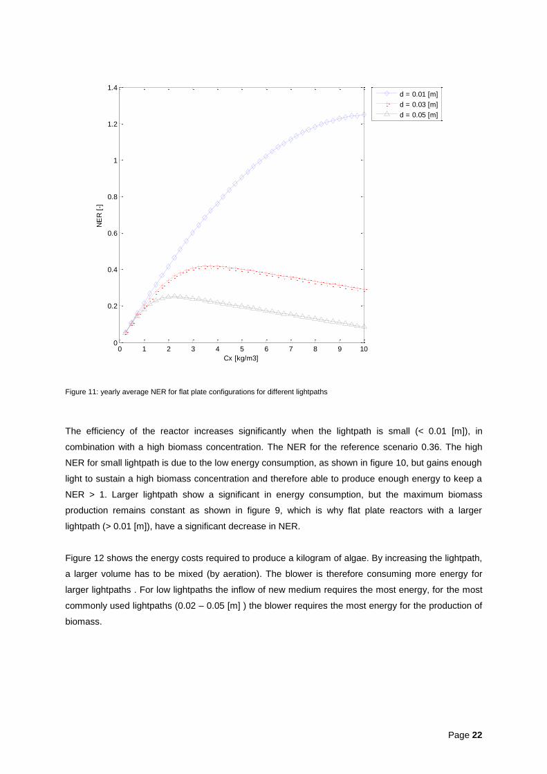
Figure 11: yearly average NER for flat plate configurations for different lightpaths
The efficiency of the reactor increases significantly when the lightpath is small (< 0.01 [m]), in
combination with a high biomass concentration. The NER for the reference scenario 0.36. The high
NER for small lightpath is due to the low energy consumption, as shown in figure 10, but gains enough
light to sustain a high biomass concentration and therefore able to produce enough energy to keep a
NER > 1. Larger lightpath show a significant in energy consumption, but the maximum biomass
production remains constant as shown in figure 9, which is why flat plate reactors with a larger
lightpath (> 0.01 [m]), have a significant decrease in NER.
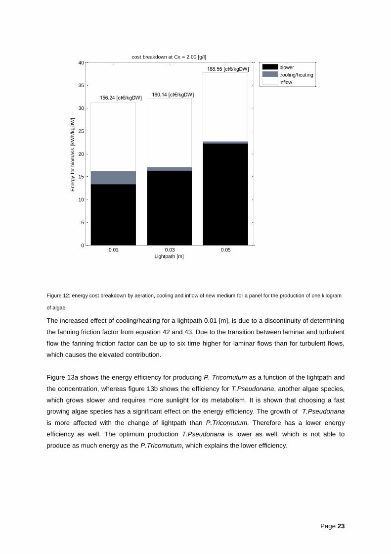
Figure 12 shows the energy costs required to produce a kilogram of algae. By increasing the lightpath,
a larger volume has to be mixed (by aeration). The blower is therefore consuming more energy for
larger lightpaths . For low lightpaths the inflow of new medium requires the most energy, for the most
commonly used lightpaths (0.02 – 0.05 [m] ) the blower requires the most energy for the production of
biomass.
0 1 2 3 4 5 6 7 8 9 100
0.2
0.4
0.6
0.8
1
1.2
1.4
Cx [kg/m3]
NE
R [
-]
d = 0.01 [m]
d = 0.03 [m]
d = 0.05 [m]
Page 23
Figure 12: energy cost breakdown by aeration, cooling and inflow of new medium for a panel for the production of one kilogram
of algae
The increased effect of cooling/heating for a lightpath 0.01 [m], is due to a discontinuity of determining
the fanning friction factor from equation 42 and 43. Due to the transition between laminar and turbulent
flow the fanning friction factor can be up to six time higher for laminar flows than for turbulent flows,
which causes the elevated contribution.
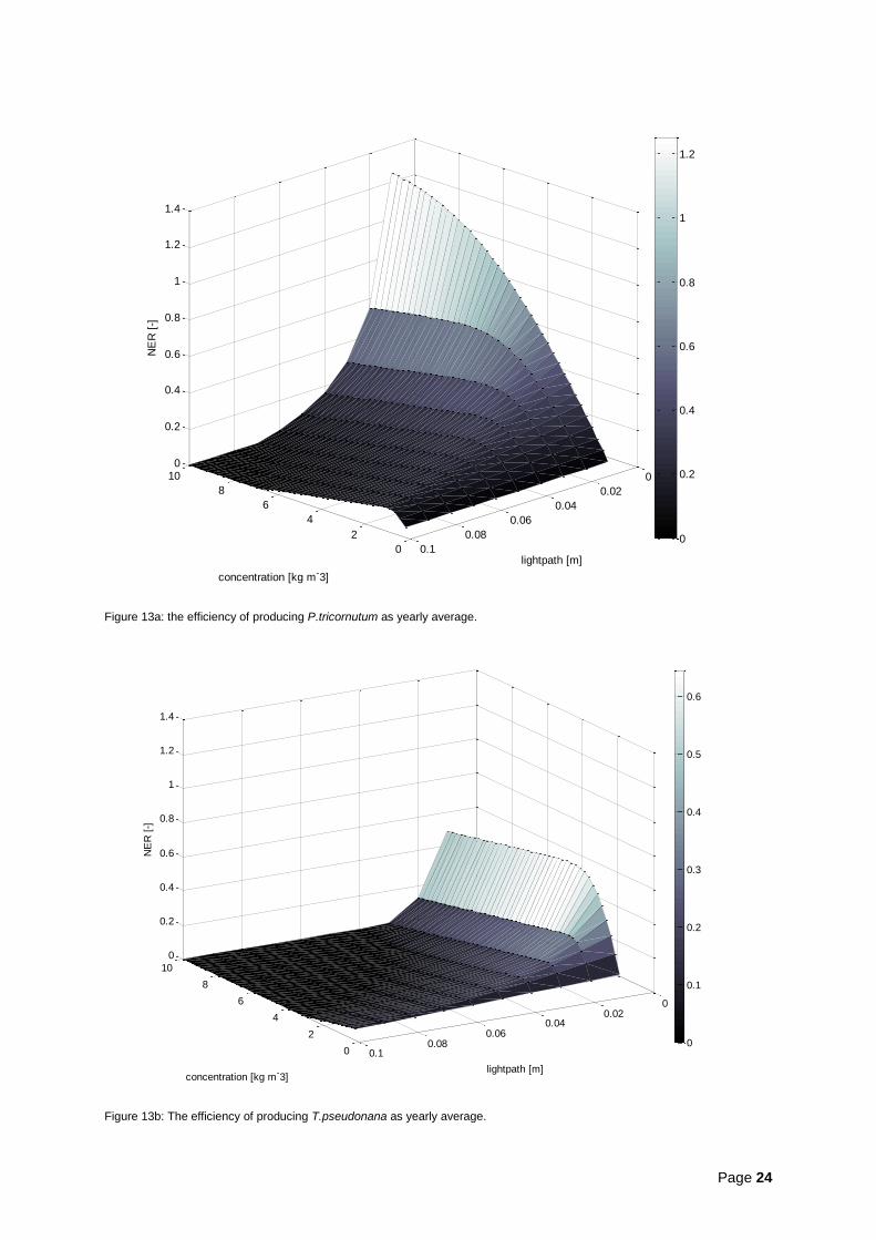
Figure 13a shows the energy efficiency for producing P. Tricornutum as a function of the lightpath and
the concentration, whereas figure 13b shows the efficiency for T.Pseudonana, another algae species,
which grows slower and requires more sunlight for its metabolism. It is shown that choosing a fast
growing algae species has a significant effect on the energy efficiency. The growth of T.Pseudonana
is more affected with the change of lightpath than P.Tricornutum. Therefore has a lower energy
efficiency as well. The optimum production T.Pseudonana is lower as well, which is not able to
produce as much energy as the P.Tricornutum, which explains the lower efficiency.
0.01 0.03 0.050
5
10
15
20
25
30
35
40
156.24 [ct€/kgDW]160.14 [ct€/kgDW]
188.55 [ct€/kgDW]E
nerg
y f
or
bio
mass [
kW
h/k
gD
W]
cost breakdown at Cx = 2.00 [g/l]
Lightpath [m]
blower
cooling/heating
inflow
Page 24
Figure 13a: the efficiency of producing P.tricornutum as yearly average.
Figure 13b: The efficiency of producing T.pseudonana as yearly average.
0
2
4
6
8
10 0
0.02
0.04
0.06
0.08
0.1
0
0.2
0.4
0.6
0.8
1
1.2
1.4
lightpath [m]
concentration [kg m-3]
NE
R [
-]
0
0.2
0.4
0.6
0.8
1
1.2
0
2
4
6
8
10
00.02
0.040.06
0.080.1
0
0.2
0.4
0.6
0.8
1
1.2
1.4
lightpath [m]concentration [kg m-3]
NE
R [
-]
0
0.1
0.2
0.3
0.4
0.5
0.6

Page 25
3.2 Results Tubular reactor The production of the tubular reactor varies with lightpath (tube radius) and the concentration as
shown in figure 14 [6].
Figure 14: yearly production of algae for a 100 [m] tube with as function of concentration and radius based on van Beveren [6]
The production is increasing with a larger lightpath, due to an increase of production volume. When
the culture becomes too dense, the production decreases sharply, due to a shortage of available light .
The optimum production of the algae shifts to the right with a decreasing radius.
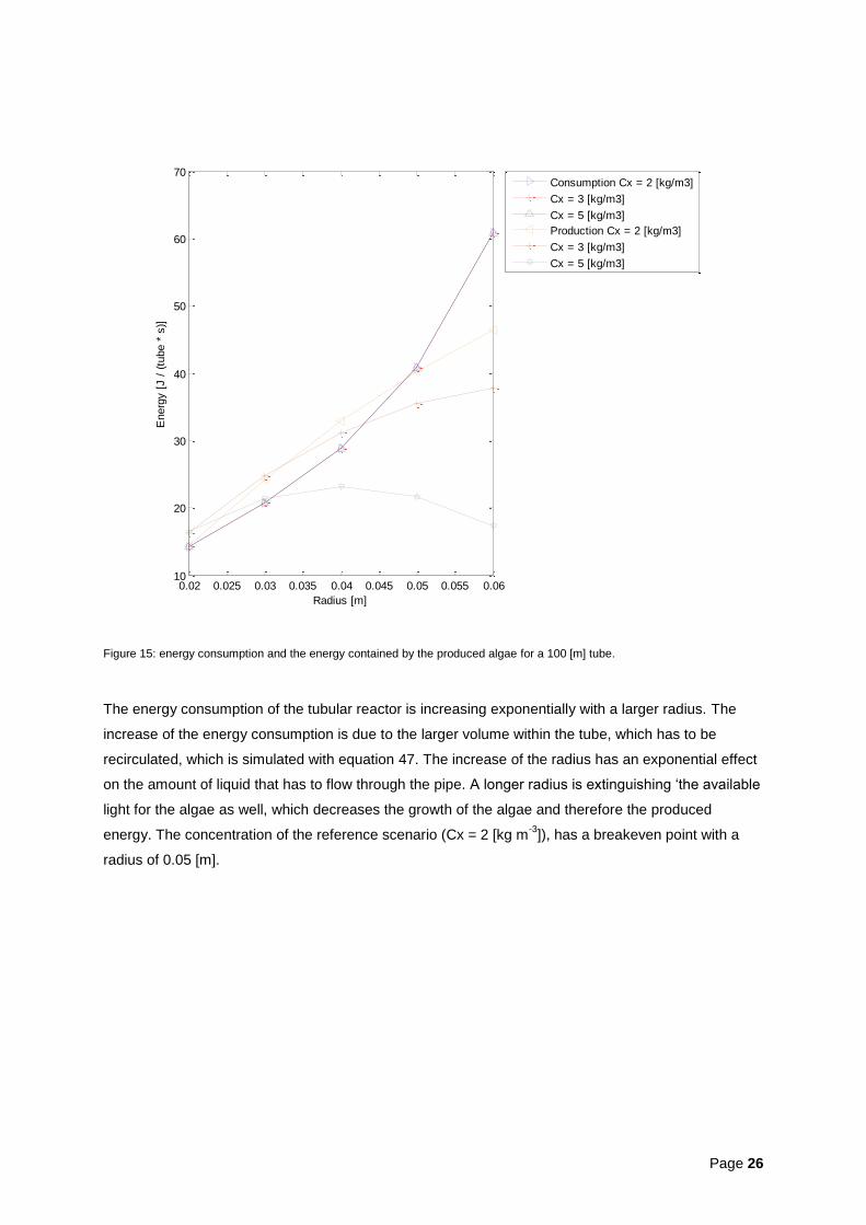
The energy required to produce algae is dependent on the volume. In figure 15 the energy required
for production and the energy contained by the produced algae is shown.
1 1.5 2 2.5 3 3.5 4 4.5 510
20
30
40
50
60
70
80
Concentration [kg/m3]
Yearly p
roduction [
Kg/(
Tube *
year)
]
r = 0.02 [m]
r = 0.03 [m]
r = 0.06 [m]
Page 26
Figure 15: energy consumption and the energy contained by the produced algae for a 100 [m] tube.
The energy consumption of the tubular reactor is increasing exponentially with a larger radius. The
increase of the energy consumption is due to the larger volume within the tube, which has to be
recirculated, which is simulated with equation 47. The increase of the radius has an exponential effect
on the amount of liquid that has to flow through the pipe. A longer radius is extinguishing ‘the available
light for the algae as well, which decreases the growth of the algae and therefore the produced
energy. The concentration of the reference scenario (Cx = 2 [kg m-3
]), has a breakeven point with a
radius of 0.05 [m].
0.02 0.025 0.03 0.035 0.04 0.045 0.05 0.055 0.0610
20
30
40
50
60
70
Radius [m]
Energ
y [
J /
(tu
be *
s)]
Consumption Cx = 2 [kg/m3]
Cx = 3 [kg/m3]
Cx = 5 [kg/m3]
Production Cx = 2 [kg/m3]
Cx = 3 [kg/m3]
Cx = 5 [kg/m3]

Page 27
In figure 16 the NER is shown with a fixed lightpath for a varying concentration.
Figure 16: yearly average NER for tubular reactor configurations with different lightpaths for a 100 [m] tube
The tubular reactor with a large lightpath (r > 0.06 [m]) has a NER <1, whereas the reactors with
smaller lightpath (r < 0.03 [m]) do show the potential to run with a NER > 1. A larger radius increases
the energy consumption of the tubular reactor, as shown in figure 15, but due to light extinction and
higher biomass concentration the algae production is decreasing. The reference scenario has a NER
of 1.3, which is above the energy neutral point. The length of the tube has an influence on the
efficiency as well, which is shown in figure 17.
1 1.5 2 2.5 3 3.5 4 4.5 50.2
0.4
0.6
0.8
1
1.2
1.4
1.6
Concentration [kg/m3]
NE
R [
-]
r = 0.02 [m]
r = 0.03 [m]
r = 0.06 [m]
Page 28
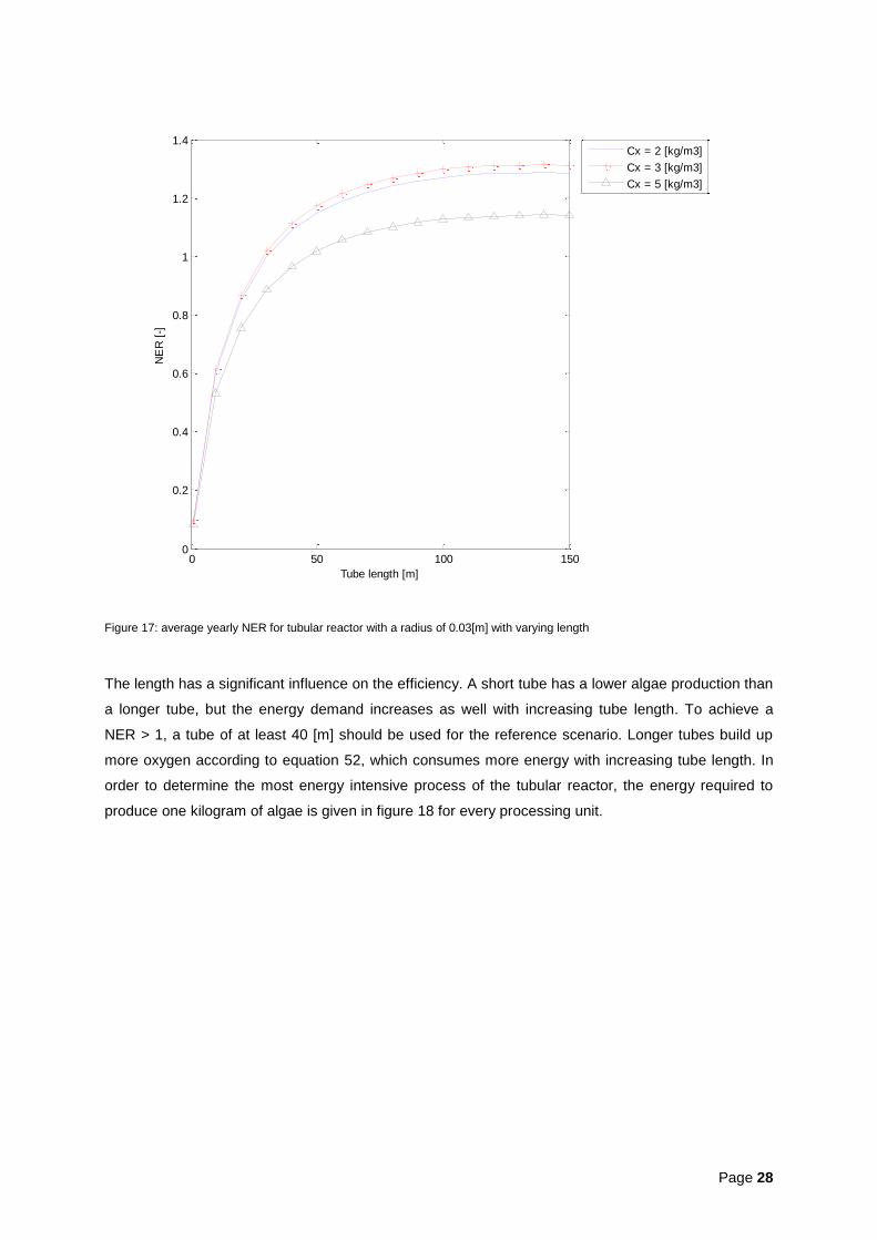
Figure 17: average yearly NER for tubular reactor with a radius of 0.03[m] with varying length
The length has a significant influence on the efficiency. A short tube has a lower algae production than
a longer tube, but the energy demand increases as well with increasing tube length. To achieve a
NER > 1, a tube of at least 40 [m] should be used for the reference scenario. Longer tubes build up
more oxygen according to equation 52, which consumes more energy with increasing tube length. In
order to determine the most energy intensive process of the tubular reactor, the energy required to
produce one kilogram of algae is given in figure 18 for every processing unit.
0 50 100 1500
0.2
0.4
0.6
0.8
1
1.2
1.4
Tube length [m]
NE
R [
-]
Cx = 2 [kg/m3]
Cx = 3 [kg/m3]
Cx = 5 [kg/m3]

Page 29
Figure 18: energy requirement for producing a kilogram algae breakdown to degassing cooling/heating processes and liquid
recirculation
Recirculation and degassing have the major contribution to the energy requirement. The cooling has
little to no influence on the energy consumption per kilogram algae, due to the large surface area the
tubular reactor has to cool. The increase of radius increases the volume of the reactor, which
increases the demand on the recirculation pump. As shown in figure 14, the production sharply
decreases with the increase of the radius, which increases the energy requirement per kilogram algae.
The energy demand of the degasser changes with the length of the reactor rather than with a larger
radius, due to the longer residence time of the algae in which more oxygen can be build up as
explained earlier. The efficiency of the effect of the tube length and the efficiency of the degasser as
shown in figure 19;
0.01 0.02 0.050
5
10
15
20
25
30
35
55.75 [ct€/kgDW] 62.34 [ct€/kgDW]
153.99 [ct€/kgDW]
Energ
y f
or
bio
mass [
Kw
h /
kgD
W]
cost breakdown at Cx = 2.00 [kg/m3]
Radius [m]
degassing
Cooler
Recirculation
Page 30
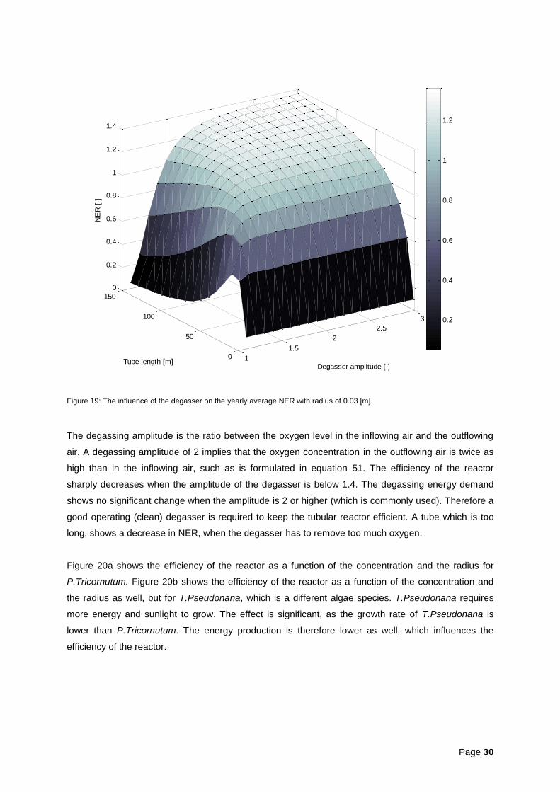
Figure 19: The influence of the degasser on the yearly average NER with radius of 0.03 [m].
The degassing amplitude is the ratio between the oxygen level in the inflowing air and the outflowing
air. A degassing amplitude of 2 implies that the oxygen concentration in the outflowing air is twice as
high than in the inflowing air, such as is formulated in equation 51. The efficiency of the reactor
sharply decreases when the amplitude of the degasser is below 1.4. The degassing energy demand
shows no significant change when the amplitude is 2 or higher (which is commonly used). Therefore a
good operating (clean) degasser is required to keep the tubular reactor efficient. A tube which is too
long, shows a decrease in NER, when the degasser has to remove too much oxygen.
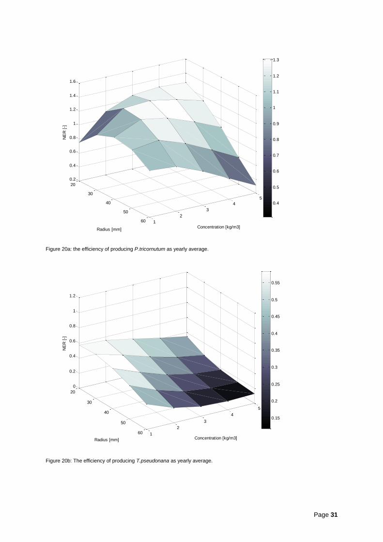
Figure 20a shows the efficiency of the reactor as a function of the concentration and the radius for
P.Tricornutum. Figure 20b shows the efficiency of the reactor as a function of the concentration and
the radius as well, but for T.Pseudonana, which is a different algae species. T.Pseudonana requires
more energy and sunlight to grow. The effect is significant, as the growth rate of T.Pseudonana is
lower than P.Tricornutum. The energy production is therefore lower as well, which influences the
efficiency of the reactor.
1
1.5
2
2.5
3
0
50
100
150
0
0.2
0.4
0.6
0.8
1
1.2
1.4
Degasser amplitude [-]Tube length [m]
NE
R [
-]
0.2
0.4
0.6
0.8
1
1.2
Page 31
Figure 20a: the efficiency of producing P.tricornutum as yearly average.
Figure 20b: The efficiency of producing T.pseudonana as yearly average.
20
30
40
50
60 1
2
3
4
5
0.2
0.4
0.6
0.8
1
1.2
1.4
1.6
Concentration [kg/m3]Radius [mm]
NE
R [
-]
0.4
0.5
0.6
0.7
0.8
0.9
1
1.1
1.2
1.3
20
30
40
50
60 1
2
3
4
5
0
0.2
0.4
0.6
0.8
1
1.2
Concentration [kg/m3]Radius [mm]
NE
R [
-]
0.15
0.2
0.25
0.3
0.35
0.4
0.45
0.5
0.55
Page 32
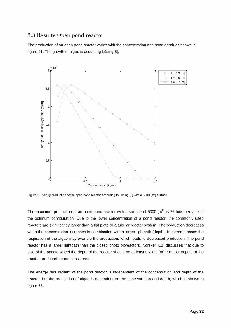
3.3 Results Open pond reactor The production of an open pond reactor varies with the concentration and pond depth as shown in
figure 21. The growth of algae is according Lösing[5],
Figure 21: yearly production of the open pond reactor according to Lösing [5] with a 5000 [m
2] surface.
The maximum production of an open pond reactor with a surface of 5000 [m2] is 26 tons per year at
the optimum configuration. Due to the lower concentration of a pond reactor, the commonly used
reactors are significantly larger than a flat plate or a tubular reactor system. The production decreases
when the concentration increases in combination with a larger lightpath (depth). In extreme cases the
respiration of the algae may overrule the production, which leads to decreased production. The pond
reactor has a larger lightpath than the closed photo bioreactors. Norsker [10] discusses that due to
size of the paddle wheel the depth of the reactor should be at least 0.2-0.3 [m]. Smaller depths of the
reactor are therefore not considered.
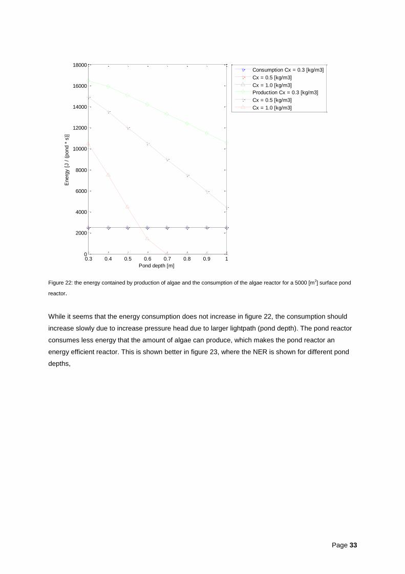
The energy requirement of the pond reactor is independent of the concentration and depth of the
reactor, but the production of algae is dependent on the concentration and depth, which is shown in
figure 22,
0 0.5 1 1.50
0.5
1
1.5
2
2.5
3x 10
4
Concentration [kg/m3]
Yearly p
roduction [
Kg/(
pond *
year)
]
d = 0.3 [m]
d = 0.5 [m]
d = 0.7 [m]
Page 33
Figure 22: the energy contained by production of algae and the consumption of the algae reactor for a 5000 [m
2] surface pond
reactor.
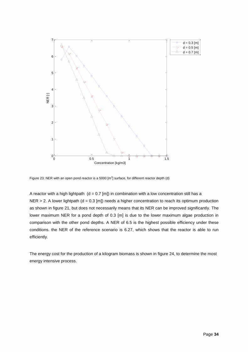
While it seems that the energy consumption does not increase in figure 22, the consumption should
increase slowly due to increase pressure head due to larger lightpath (pond depth). The pond reactor
consumes less energy that the amount of algae can produce, which makes the pond reactor an
energy efficient reactor. This is shown better in figure 23, where the NER is shown for different pond
depths,
0.3 0.4 0.5 0.6 0.7 0.8 0.9 10
2000
4000
6000
8000
10000
12000
14000
16000
18000
Pond depth [m]
Energ
y [
J /
(pond *
s)]
Consumption Cx = 0.3 [kg/m3]
Cx = 0.5 [kg/m3]
Cx = 1.0 [kg/m3]
Production Cx = 0.3 [kg/m3]
Cx = 0.5 [kg/m3]
Cx = 1.0 [kg/m3]
Page 34
Figure 23: NER with an open pond reactor is a 5000 [m2] surface, for different reactor depth (d)
A reactor with a high lightpath (d = 0.7 [m]) in combination with a low concentration still has a
NER > 2. A lower lightpath (d = 0.3 [m]) needs a higher concentration to reach its optimum production
as shown in figure 21, but does not necessarily means that its NER can be improved significantly. The
lower maximum NER for a pond depth of 0.3 [m] is due to the lower maximum algae production in
comparison with the other pond depths. A NER of 6.5 is the highest possible efficiency under these
conditions. the NER of the reference scenario is 6.27, which shows that the reactor is able to run
efficiently.
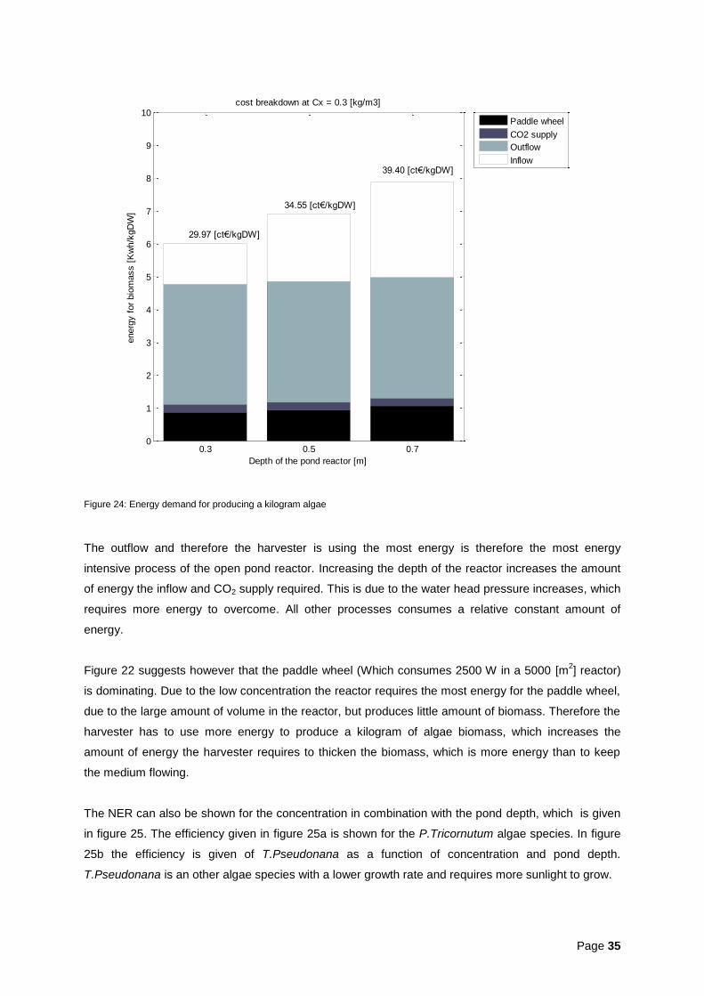
The energy cost for the production of a kilogram biomass is shown in figure 24, to determine the most
energy intensive process.
0 0.5 1 1.50
1
2
3
4
5
6
7
Concentration [kg/m3]
NE
R [
-]
d = 0.3 [m]
d = 0.5 [m]
d = 0.7 [m]
Page 35
Figure 24: Energy demand for producing a kilogram algae
The outflow and therefore the harvester is using the most energy is therefore the most energy
intensive process of the open pond reactor. Increasing the depth of the reactor increases the amount
of energy the inflow and CO2 supply required. This is due to the water head pressure increases, which
requires more energy to overcome. All other processes consumes a relative constant amount of
energy.
Figure 22 suggests however that the paddle wheel (Which consumes 2500 W in a 5000 [m2] reactor)
is dominating. Due to the low concentration the reactor requires the most energy for the paddle wheel,
due to the large amount of volume in the reactor, but produces little amount of biomass. Therefore the
harvester has to use more energy to produce a kilogram of algae biomass, which increases the
amount of energy the harvester requires to thicken the biomass, which is more energy than to keep
the medium flowing.
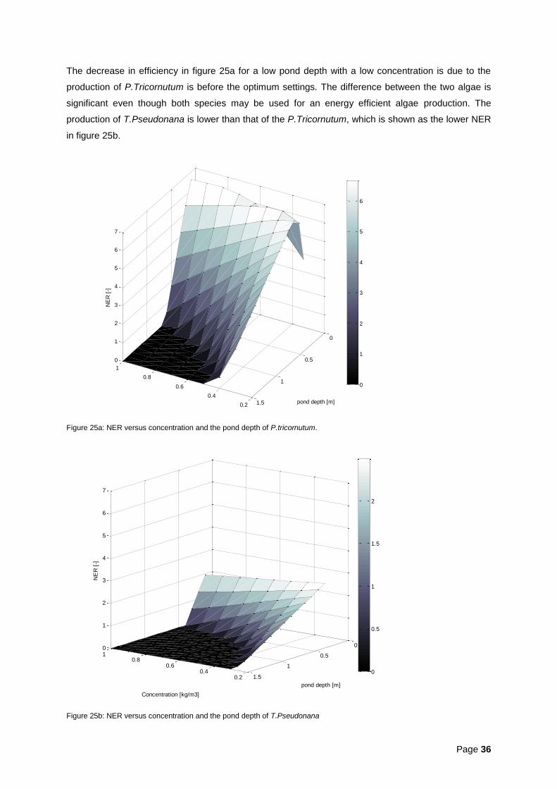
The NER can also be shown for the concentration in combination with the pond depth, which is given
in figure 25. The efficiency given in figure 25a is shown for the P.Tricornutum algae species. In figure
25b the efficiency is given of T.Pseudonana as a function of concentration and pond depth.
T.Pseudonana is an other algae species with a lower growth rate and requires more sunlight to grow.
0.3 0.5 0.70
1
2
3
4
5
6
7
8
9
10
energ
y f
or
bio
mass [
Kw
h/k
gD
W]
cost breakdown at Cx = 0.3 [kg/m3]
Depth of the pond reactor [m]
29.97 [ct€/kgDW]
34.55 [ct€/kgDW]
39.40 [ct€/kgDW]
Paddle wheel
CO2 supply
Outflow
Inflow
Page 36
The decrease in efficiency in figure 25a for a low pond depth with a low concentration is due to the
production of P.Tricornutum is before the optimum settings. The difference between the two algae is
significant even though both species may be used for an energy efficient algae production. The
production of T.Pseudonana is lower than that of the P.Tricornutum, which is shown as the lower NER
in figure 25b.
Figure 25a: NER versus concentration and the pond depth of P.tricornutum.
Figure 25b: NER versus concentration and the pond depth of T.Pseudonana
0.2
0.4
0.6
0.8
1
0
0.5
1
1.5
0
1
2
3
4
5
6
7
pond depth [m]
Concentration [kg/m3]
NE
R [
-]
0
1
2
3
4
5
6
0.20.4
0.60.8
1
0
0.5
1
1.5
0
1
2
3
4
5
6
7
pond depth [m]
Concentration [kg/m3]
NE
R [
-]
0
0.5
1
1.5
2

Page 37
Page 38
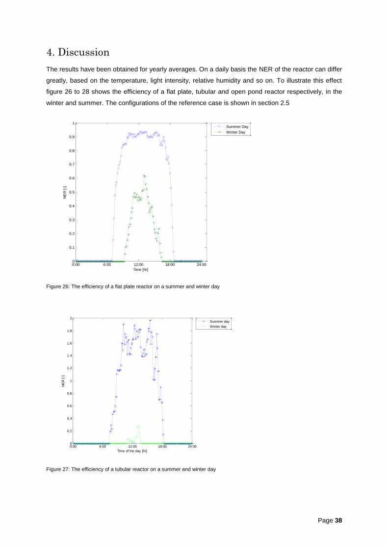
4. Discussion The results have been obtained for yearly averages. On a daily basis the NER of the reactor can differ
greatly, based on the temperature, light intensity, relative humidity and so on. To illustrate this effect
figure 26 to 28 shows the efficiency of a flat plate, tubular and open pond reactor respectively, in the
winter and summer. The configurations of the reference case is shown in section 2.5
Figure 26: The efficiency of a flat plate reactor on a summer and winter day
Figure 27: The efficiency of a tubular reactor on a summer and winter day
0:00 6:00 12:00 18:00 24:000
0.1
0.2
0.3
0.4
0.5
0.6
0.7
0.8
0.9
1
Time [hr]
NE
R [
-]
Summer Day
Winter Day
0:00 6:00 12:00 18:00 24:000
0.2
0.4
0.6
0.8
1
1.2
1.4
1.6
1.8
2
Time of the day [hr]
NE
R [
-]
Summer day
Winter day
Page 39
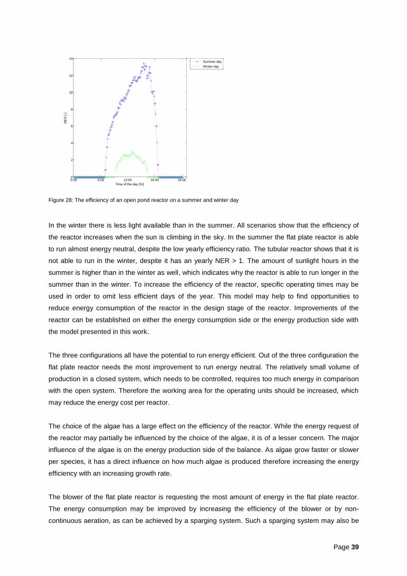
Figure 28: The efficiency of an open pond reactor on a summer and winter day
In the winter there is less light available than in the summer. All scenarios show that the efficiency of
the reactor increases when the sun is climbing in the sky. In the summer the flat plate reactor is able
to run almost energy neutral, despite the low yearly efficiency ratio. The tubular reactor shows that it is
not able to run in the winter, despite it has an yearly NER > 1. The amount of sunlight hours in the
summer is higher than in the winter as well, which indicates why the reactor is able to run longer in the
summer than in the winter. To increase the efficiency of the reactor, specific operating times may be
used in order to omit less efficient days of the year. This model may help to find opportunities to
reduce energy consumption of the reactor in the design stage of the reactor. Improvements of the
reactor can be established on either the energy consumption side or the energy production side with
the model presented in this work.
The three configurations all have the potential to run energy efficient. Out of the three configuration the
flat plate reactor needs the most improvement to run energy neutral. The relatively small volume of
production in a closed system, which needs to be controlled, requires too much energy in comparison
with the open system. Therefore the working area for the operating units should be increased, which
may reduce the energy cost per reactor.
The choice of the algae has a large effect on the efficiency of the reactor. While the energy request of
the reactor may partially be influenced by the choice of the algae, it is of a lesser concern. The major
influence of the algae is on the energy production side of the balance. As algae grow faster or slower
per species, it has a direct influence on how much algae is produced therefore increasing the energy
efficiency with an increasing growth rate.
The blower of the flat plate reactor is requesting the most amount of energy in the flat plate reactor.
The energy consumption may be improved by increasing the efficiency of the blower or by non-
continuous aeration, as can be achieved by a sparging system. Such a sparging system may also be
0:00 6:00 12:00 18:00 24:000
2
4
6
8
10
12
14
Time of the day [hr]
NE
R [
-]
Summer day
Winter day
Page 40
used over multiple plates, which may reduce the energy cost even further. Using the blower only part
of the day may also result in improved efficiently. Linear increasing of downtime of the blower will shift
the energy consumption line of figure 10 downwards. The NER will then increase, but the algae
growth may be decrease slightly, due to inhibition by oxygen.
Less energy consumption in a tubular reactor is harder to achieve, as there is not much to gain with an
more efficient degasser and the energy consumption is constrained by the recirculation. A faster
growing (or genetically modified) algae, gives more space to improve the efficiency ratio. A pond
reactor is already energy efficient, but requires much land to run. Energy wise there is no need to
improve the pond reactor, although a faster growing algae species may be able to improve the NER to
higher levels.
The NER indicates that the flat plate reactor requires more energy than it produces. However, this
does not indicate that the flat plate reactor is not feasible. The NER is of great importance to the bulk
chemistry sector, such as the production of biodiesel. In the pharmaceutical field, such as the
production of ω 3,6 and 9 fatty acids, the selling prices are much higher, which may improve the
feasibility of any configuration.
Norsker [10] published energy costs for the production of one kilogram algae in three configurations.
His estimates to produce one kilogram algae are € 0.24 , € 0.57 and € 2.43 for an open pond reactor,
tubular reactor and a flat plate reactor respectively. These figures represent the energy costs only.
This work determines the cost to produce a kilogram algae to be €0.29, €0.62 and €1.60, for an open
pond, tubular and a flat plate reactor respectively. The costs presented in this work differ from these
figures partly due to a faster growing algae species and due to different estimates for energy
consumption. The production of algae in the flat plate reactor is 2.5 times higher in this work, which
reduces the running energy cost per algae. Furthermore, the inflow of new medium enters from the
bottom of the reactor, which gives an additional energy requirement due to the pressure head of
water. Lastly, Norsker uses some processing equipment for multiple reactors. This is not taken into
account in this work.
Cheng-Wu et al.[11] shows that for the cultivation of Nannochloropsis sp. in a 2000 L flat plate reactor
with a lightpath of 10 cm, the energy costs take up to 6.5% of the total costs. In order to achieve this,
the process units are only running a specific amount of time per day. In this work all process units that
depends on the growth of the algae, such as the degasser, are consuming only energy when there is
a positive production. This means that the operating hours are longer in the summer than in the winter
and the process units are switched off in the evening. At this point there is no influent as well, as it is
assumed that the respiration of algae is small and used to supply nutrients to the remaining algae
culture.
Page 41
For the closed reactor systems it is assumed that the evaporation cooling conditions are optimal. This
implies that the air has no water vapour and therefore the relative humidity of the environment is 0.
The relative humidity on the reactor itself should (in ideal conditions) be 1, to give the maximum
potential to remove the heat. In practise, the relative humidity of air lowers this potential. If the relative
humidity of the air is taken into account of the cooling flow, which is formulated in equation 37, the
equation may be reformulated as[18],
(
) [ ( ) ] (75)
Where is the ambient temperature, is the required temperature for the reactor, is the
evaporation energy per kilogram water, (
) is the ratio between the evaporative and convective
transfer functions, ( ) is the density of water on the reactor and is the density of air at the
specific humidity. When the relative humidity is high re-condensation on the reactor can occur. The
cooler is not able to remove the excess heat, which is a limitation for the cooling. Therefore in humid
countries, such as in western Europe, evaporative cooling is a particularly inefficient cooling method,
especially during relatively wet and cold periods, as spring autumn and winter. The excess amount of
heat which would be removed by evaporation would now be removed by convective cooling, which
creates an additional layer where sunlight has to go through. The intensity of sunlight may be less
when it reaches the algae, therefore reducing the amount of growth, making the closed
photobioreactor less efficient.
Page 42
5. Conclusion A mathematical model has been made to analyse in the energy efficiency of a flat plate, tubular and
an open pond reactor. With this model the netto energy ratio (NER) is calculated for various algae
photobioreactor designs. This NER analysis can be done for several time scales, from efficiency on
one day to a year round average. It is shown that all the reactor configurations have different
performance in NER which depends changes in the concentration and lightpath. The intensity of the
sun has a significant effect on the efficiency of the reactors, which gives higher NER in the summer
than in the winter and at noon rather than the morning.
The flat plate, tubular and open pond reactor have been simulated to show the effects of changing the
input and design variables. For standard photobioreactors NER is 0.36 for a flat plate reactor, 1.3 for a
tubular reactor and 6.27 for the open pond reactor. This result has been obtained for environmental
conditions in the Netherlands and for the P.Tricornutum algae species. The choice of the algae is
important as faster growing algae produce more biomass, which directly influence the NER positively.
For the most commonly used lightpaths (0.02 – 0.05 [m]) in flat plate reactors, the aeration uses the
most energy, which increases linearly with the increase of volume. A small lightpath (< 0.01 [m]) in
combination with a high biomass concentration provides a NER > 1.
P.Tricornutum does not grow fast enough to provide enough energy to sustain an energy neutral
configuration for a flat plate reactor, therefore a faster growing algae should be employed. Other
methods for aeration, such as sparging, should be investigated in order to reduce the energy
consumption. A combination of a faster growing algae species and energy consumption reduction will
improve the efficiency of the flat plate reactor, which is currently not able to run energy neutral yet.
A standard tubular reactor is operates with a positive NER. The liquid recirculation demands the most
energy. In comparison with the flat plate reactor there are less options in order to reduce the energy
and therefore increasing the growth rate of algae has the best opportunity to make this reactor more
efficient.
The open pond reactor has an overall efficiency NER > 1, which means that the reactor is able to run
energy efficient. The reference scenario has an efficiency of 6.27. The consumption of the open pond
reactor is fixed due to the dominating energy cost of the centrifuge. Reduction of the paddle wheel and
centrifuge costs may increase the NER, to increase the efficiency even further.

Page 43
Page 44
References
Literature
1. Naik, S.N., et al., Production of first and second generation biofuels: A comprehensive review. Renewable and Sustainable Energy Reviews. 14(2): p. 578-597.
2. Nigam, P.S. and A. Singh, Production of liquid biofuels from renewable resources. Progress in Energy and Combustion Science, 2011. 37(1): p. 52-68.
3. Chisti, Y., Biodiesel from microalgae. Biotechnology Advances, 2007. 25: p. 294-306. 4. Slegers, P.M., et al., Design scenarios for flat panel photobioreactors. Applied Energy, 2011.
88(10): p. 3342-3353. 5. Lösing, M.B., Modelling & Simulating microalgae production in an open pond reactor, in
System and Control2011, Wageningen UR: Wageningen. 6. van Beveren, P.J.M., Algal growth in horizontal tubular reactor, in System and Control 2011,
Wageningen UR: Wageningen. 7. Owen, N.A., O.R. Inderwildi, and D.A. King, The status of conventional world oil reserves—
Hype or cause for concern? Energy Policy, 2010. 38(8): p. 4743-4749. 8. Wijffels, R.H. and M.J. Barbosa, An Outlook on Microalgal biofuels. Science, 2010. 329(5993):
p. 796-799. 9. Lehr, F. and C. Posten, Closed photo-bioreactors as tools for biofuel production. Current
Opinion in Biotechnology, 2009. 20(3): p. 280-285. 10. Norsker, N.H., et al., Microalgal production - A close look at the economics. Biotechnology
Advances, 2011. 29(1): p. 24-27. 11. Cheng-Wu, Z., et al., An industrial-size flat plate glass reactor for mass production of
Nannochloropsis sp. (Eustigmatophyceae). Aquaculture, 2001. 195(1-2): p. 35-49. 12. Geider, R.J. and H.L. MacIntyre, A dynamic model of photoadaptation in phytoplankton.
Limnology and Oceanography, 1996. 41(1): p. 1-15. 13. Bird, R.B., W.E. Stewart, and E.N. Lightfoot, Transport Phenomena1960: Wiley International. 14. Geankoplis, C.J., Transport Processes and separation unit principles (includes unit
operations). 4th ed2003: Prentice Hall. 15. Acién Fernández, F.G., et al., Airlift-driven external-loop tubular photobioreactors for outdoor
production of microalgae: assessment of design and performance. Chemical Engineering Science, 2001. 56(8): p. 2721-2732.
16. Molina, E., et al., Tubular photobioreactor design for algal cultures. Journal of Biotechnology, 2001. 92(2): p. 113-131.
17. Knap, W., measurements of radiation at station Cabauw., KNMI, Editor 2009: De Bilt. 18. Incropera, et al., Fundamentals of Heat and Mass Transfer. 6th ed2007: John Wiley & Sons. 19. Thomas, W.H., et al., Yields, photosynthetic efficiencies and proximate composition of dense
marine microalgal cultures. I. Introduction and Phaeodactylum tricornutum experiments. Biomass, 1984. 5(3): p. 181-209.

Page 45

Page 46
Acknowledgements This report is the product of hard work and a lot of stress and would not be completed without the help
of various people, which I would like to thank for their contribution.
Ellen Slegers for the opportunity for taking this project and supervision throughout the year. Ton van
Boxtel, for his endless patience, correcting this document, supervision and thoughts. The science
group SCO for taking me as one of them for almost a year, especially Rachel van Ooteghem, for
solving a lot of Matlab problems. The students of SCO, which came and go from my room, specifically
Peter van Beveren and Martin Lösing, for their help with the startup of the project and their data from
their projects. My numerous friends for dealing with me in desperate times. Last but not the least, my
parents for always believing in me.
I would like to extend my gratitude to the AlgaePARC project of Wageningen University for providing
the pictures used on the front page and in figure 1 and Marcel Alderlieste for his correctional work on
spelling and grammar.

Page 47
Page 48
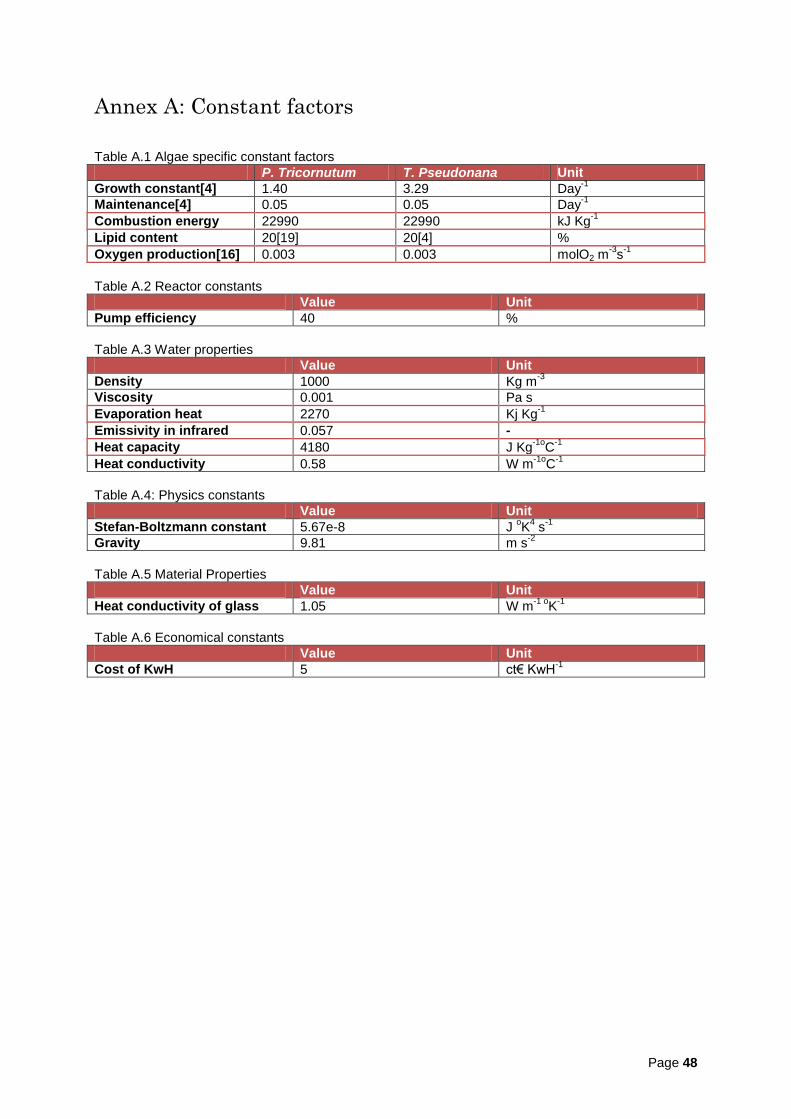
Annex A: Constant factors Table A.1 Algae specific constant factors
P. Tricornutum T. Pseudonana Unit
Growth constant[4] 1.40 3.29 Day-1
Maintenance[4] 0.05 0.05 Day-1
Combustion energy 22990 22990 kJ Kg-1
Lipid content 20[19] 20[4] %
Oxygen production[16] 0.003 0.003 molO2 m-3
s-1
Table A.2 Reactor constants
Value Unit
Pump efficiency 40 %
Table A.3 Water properties
Value Unit
Density 1000 Kg m-3
Viscosity 0.001 Pa s
Evaporation heat 2270 Kj Kg-1
Emissivity in infrared 0.057 -
Heat capacity 4180 J Kg-1o
C-1
Heat conductivity 0.58 W m-1o
C-1
Table A.4: Physics constants
Value Unit
Stefan-Boltzmann constant 5.67e-8 J oK
4 s
-1
Gravity 9.81 m s-2
Table A.5 Material Properties
Value Unit
Heat conductivity of glass 1.05 W m-1 o
K-1
Table A.6 Economical constants
Value Unit
Cost of KwH 5 ct€ KwH-1

Page 49
Page 50
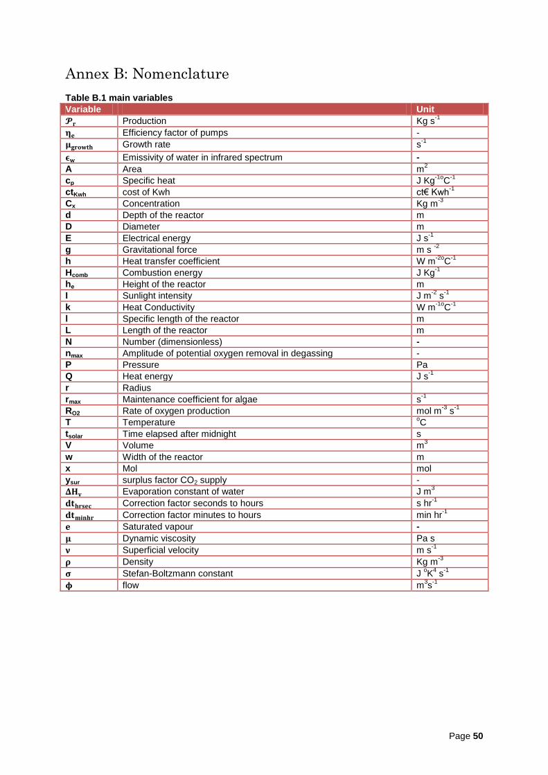
Annex B: Nomenclature Table B.1 main variables
Variable Unit
Production Kg s-1
Efficiency factor of pumps -
Growth rate s-1
Emissivity of water in infrared spectrum -
A Area m2
cp Specific heat J Kg-1o
C-1
ctKwh cost of Kwh ct€ Kwh-1
Cx Concentration Kg m-3
d Depth of the reactor m
D Diameter m
E Electrical energy J s-1
g Gravitational force m s -2
h Heat transfer coefficient W m-2o
C-1
Hcomb Combustion energy J Kg-1
he Height of the reactor m
I Sunlight intensity J m-2
s-1
k Heat Conductivity W m-1o
C-1
l Specific length of the reactor m
L Length of the reactor m
N Number (dimensionless) -
nmax Amplitude of potential oxygen removal in degassing -
P Pressure Pa
Q Heat energy J s-1
r Radius
rmax Maintenance coefficient for algae s-1
RO2 Rate of oxygen production mol m-3
s-1
T Temperature oC
tsolar Time elapsed after midnight s
V Volume m3
w Width of the reactor m
x Mol mol
ysur surplus factor CO2 supply -
Evaporation constant of water J m3
Correction factor seconds to hours s hr-1
Correction factor minutes to hours min hr-1
Saturated vapour -
Dynamic viscosity Pa s
Superficial velocity m s-1
Density Kg m-3
Stefan-Boltzmann constant J oK
4 s
-1
flow m3s
-1
Page 51
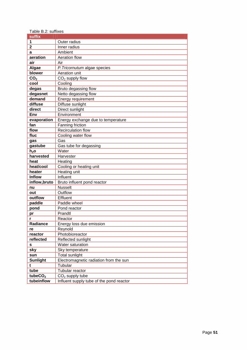
Table B.2: suffixes
suffix
1 Outer radius
2 Inner radius
a Ambient
aeration Aeration flow
air Air
Algae P.Tricornutum algae species
blower Aeration unit
CO2 CO2 supply flow
cool Cooling
degas Bruto degassing flow
degasnet Netto degassing flow
demand Energy requirement
diffuse Diffuse sunlight
direct Direct sunlight
Env Environment
evaporation Energy exchange due to temperature
fan Fanning friction
flow Recirculation flow
fluc Cooling water flow
gas Gas
gastube Gas tube for degassing
h2o Water
harvested Harvester
heat Heating
heat/cool Cooling or heating unit
heater Heating unit
Inflow Influent
inflow,bruto Bruto influent pond reactor
nu Nusselt
out Outflow
outflow Effluent
paddle Paddle wheel
pond Pond reactor
pr Prandtl
r Reactor
Radiance Energy loss due emission
re Reynold
reactor Photobioreactor
reflected Reflected sunlight
s Water saturation
sky Sky temperature
sun Total sunlight
Sunlight Electromagnetic radiation from the sun
t Tubular
tube Tubular reactor
tubeCO2 CO2 supply tube
tubeinflow Influent supply tube of the pond reactor

Page 52