modelling of flowability measurement of cohesive powders
TRANSCRIPT

Modelling of Flowability Measurement of Cohesive Powders Using Small
Quantities
By
Massih Pasha
Submitted in accordance with the requirements for the degree of
Doctor of Philosophy
The University of Leeds
School of Process, Environmental and Materials Engineering
February 2013
The candidate confirms that the work submitted is his own, except where work which
has formed part of jointly authored publications has been included. The contribution of
the candidate and the other authors to this work has been explicitly indicated below. The
candidate confirms that appropriate credit has been given within the thesis where
reference has been made to the work of others.
This copy has been supplied on the understanding that it is copyright material and that
no quotation from the thesis may be published without proper acknowledgment.
© 2013 The University of Leeds and Massih Pasha

Chapter 5 of this thesis has already been published in Powder Technology (Pasha et al.
2013). The analyses, discussions and conclusions were all done by Massih Pasha. Other
authors of this publication provided feedback and guidance.
M. Pasha, C. Hare, A. Hassanpour, and M. Ghadiri, “Analysis of ball
indentation on cohesive powder beds using distinct element modelling”, Powder
Technology, vol. 233, pp. 80-90, 2013.

Acknowledgments
While working on this work I have benefited from the support and help of many people,
few of whom I would like to thank here.
First and foremost I should express my highest degree of appreciation to my project
supervisors Professor Mojtaba Ghadiri and Dr Ali Hassanpour whose insights,
enthusiasm and constant unconditional support were key to my success.
The financial support from the Engineering and Physical Science Research Council
(EPSRC), National Nuclear Laboratory (NNL) and Sellafield Ltd is gratefully
appreciated. I would like to acknowledge the support and constructive comments from
Dr Terry Semeraz of NNL and Dr Robert Stephen of Sellafield Ltd. I am also thankful
to Mr Umair Zafar and Dr Colin Hare for sharing thoughts and invaluable assistance. Dr
Colin Hare’s effort and time on proof reading this thesis are greatly appreciated. I would
like to convey thanks to Dr Afsheen Zarrebini for sharing 9 years of student life with
me and introducing me to the research group. I also would like to thank my colleagues
and friends, Dr Hossein Ahmadian, Dr Graham Calvert, Mr Selasi Dogbe and Miss
Nadia Haerizadeh-Yazdi for their support and encouragement.
Last but by no means least, I would like to convey an immeasurable amount of gratitude
to my dearest parents, Mrs Alam Zarrehbini and Mr Ahmadgholi Pasha, and to my
sister and brother, Miss Leila Pasha and Mr Mehrdad Pasha, for their unconditional love
and support throughout the numerous ups and downs of my life.

To My Dear Parents

Abstract
The characterisation of cohesive powders for flowability is often required for reliable
design and consistent operation of powder processes. This is commonly achieved by the
unconfined compression test or shear test, but these techniques require a relatively large
amount of powder and are limited to large pre-consolidation loads. There are a number
of industrial cases where these tests are not applicable because small amounts of
powders have to be handled and processed, such as filling and dosing of small quantities
of powder in capsules and dispersion in dry powder inhalers. In other cases, the
availability of testing powders could be a limiting issue. It has been shown by
Hassanpour and Ghadiri (2007) that under certain circumstances, indentation on a
cohesive powder bed by a blunt indenter can give a measure of the resistance to powder
flow, which is related to flowability. However, the specification of the operation
window in terms of sample size, penetration depth, indenter properties and strain rate
has yet to be fully analysed. In the present work, the ball indentation process is analysed
by numerical simulations using the Distinct Element Method (DEM). The flow
resistance of the assembly, commonly termed hardness, is evaluated for a range of
sample quantities and operation variables. It is shown that a minimum bed height of 20
particle diameters is required in order to achieve reliable measurements of hardness. A
sensitivity analysis of indenter size reveals that small indenters with diameters less than
16 times the particle diameter exhibit fluctuations in powder flow stress measurements,
which do not represent shear deformation. The penetration depth should be sufficiently
large to cause notable bed shear deformation. It is found that this minimum penetration
depth is approximately equal to 10% of the indenter radius. The hardness measurements
are found to be independent of indenter stiffness within the wide range investigated.

The friction between the indenter and the particles slightly increases the hardness,
although its influence on the internal stresses is negligible. Cubic and cylindrical
indenters measure significantly larger hardness value compared to the spherical indenter.
Increasing the inter-particle friction and cohesion results in higher hardness values and
internal stresses, due to the increase in resistance to shear deformation. Simulations at a
range of indenter velocities confirm that the ball indentation technique can be used to
analyse powder flowability over a wide range of shear rates.

i
Contents
Acknowledgments .............................................................................................................. I
Abstract ............................................................................................................................ II
Contents ............................................................................................................................. i
List of Figures .................................................................................................................. vi
List of Tables................................................................................................................... xv
Nomenclature ................................................................................................................. xvi
Latin Characters .......................................................................................................... xvi
Greek Characters.......................................................................................................... xx
CHAPTER 1 Introduction ............................................................................................. 1
Powder flowability ............................................................................................. 1 1.1
Objectives and structure of the thesis ................................................................. 3 1.2
CHAPTER 2 Flowability Measurement Techniques .................................................... 6
Uniaxial compression test .................................................................................. 6 2.1
Representation of stresses using Mohr’s stress circles ............................... 7 2.1.1
Classification of powders based on their flow behaviour ........................... 9 2.1.2
Shear testing ..................................................................................................... 11 2.2
Representation of stresses using Mohr’s stress circles ............................. 13 2.2.1
Flowability measurements at low consolidation stresses and tensile regimes . 15 2.3
Shear testers .............................................................................................. 15 2.3.1
Sevilla powder tester ................................................................................. 16 2.3.2
Angle of repose ......................................................................................... 20 2.3.3
Vibrating capillary method ....................................................................... 21 2.3.4

ii
Ball indentation ......................................................................................... 24 2.3.5
Comparison of flowability measurement techniques ....................................... 33 2.4
CHAPTER 3 Distinct Element Method (DEM) .......................................................... 37
Time-step .......................................................................................................... 38 3.1
Motion calculations .......................................................................................... 39 3.2
Contact and non-contact forces ........................................................................ 40 3.3
Van der Waals forces ................................................................................ 40 3.3.1
Liquid bridges ........................................................................................... 41 3.3.2
Electrostatics ............................................................................................. 42 3.3.3
Contact Force Models ...................................................................................... 42 3.4
Elastic contacts .......................................................................................... 43 3.4.1
3.4.1.1 Linear spring contact model .............................................................. 43
3.4.1.2 Hertz normal contact model ............................................................... 45
3.4.1.3 Mindlin and Deresiewicz’s tangential contact model ........................ 45
3.4.1.4 Mindlin’s no-slip tangential contact model ....................................... 49
3.4.1.5 Di Renzo and Di Maio’s no-slip tangential contact model ................ 51
Elasto-plastic contacts ............................................................................... 53 3.4.2
3.4.2.1 Thornton’s elasto-plastic normal contact model ................................ 53
3.4.2.2 Vu-Quoc and Zhang’s elasto-plastic normal contact model .............. 56
3.4.2.3 Walton and Braun normal elasto-plastic model ................................. 60
3.4.2.4 Tangential force in elasto-plastic contacts ......................................... 63
Elastic-adhesive contacts .......................................................................... 63 3.4.3
3.4.3.1 JKR elastic-adhesion normal contact model ...................................... 63

iii
3.4.3.2 Savkoor and Briggs’ tangential model for elastic-adhesive contacts 65
3.4.3.3 Thornton and Yin’s tangential model for elastic-adhesive contacts .. 66
3.4.3.4 DMT elastic-adhesive normal contact model .................................... 68
3.4.3.5 Matuttis and Schinner’s elastic-adhesive normal contact model ....... 69
Elasto-plastic and adhesive contacts ......................................................... 71 3.4.4
3.4.4.1 Thornton and Ning’s elasto-plastic and adhesive normal contact
model 71
3.4.4.2 Ning’s elasto-plastic and adhesive tangential contact model ............ 75
3.4.4.3 Tomas’ elasto-plastic and adhesive normal contact model ............... 77
3.4.4.4 Tomas’ elasto-plastic and adhesive tangential contact model ........... 81
3.4.4.5 Luding’s (2008) elasto-plastic and adhesive normal contact model.. 81
3.4.4.6 Luding’s (2008) elasto-plastic and adhesive tangential contact model
84
Particle shape .................................................................................................... 84 3.5
Reduction of rotational freedom of spheres .............................................. 85 3.5.1
Clumped spheres ....................................................................................... 86 3.5.2
Polyhedral shapes ...................................................................................... 88 3.5.3
Continuous super-quadric function ........................................................... 90 3.5.4
Discrete function representation (DFP) .................................................... 91 3.5.5
Digitisation ................................................................................................ 92 3.5.6
CHAPTER 4 A New Linear Model for Elasto-Plastic and Adhesive Contacts in DEM
94
Normal contacts ................................................................................................ 94 4.1

iv
Load-dependent pull-off force .................................................................. 97 4.1.1
Sensitivity of plastic pull-off force to contact properties .......................... 99 4.1.2
Impact, rebound and critical sticking velocities ...................................... 103 4.1.3
Linearisation of locus of pull-off force ................................................... 111 4.1.4
Comparison of the proposed model with Luding’s, and Thornton and 4.1.5
Ning’s [15] models ................................................................................................. 113
Normal contact damping ................................................................................ 123 4.2
Tangential model ............................................................................................ 124 4.3
Sensitivity analysis of the proposed model parameters .................................. 124 4.4
Conclusions .................................................................................................... 130 4.5
CHAPTER 5 Numerical Analysis of Minimum Sample Size and Indenter Size Range
in Ball Indentation Method by DEM ............................................................................ 132
DEM Simulation of the indentation process .................................................. 132 5.1
Contact models ........................................................................................ 132 5.1.1
Stress calculation ..................................................................................... 134 5.1.2
Simulation properties .............................................................................. 135 5.1.3
Results and discussions .................................................................................. 137 5.2
Conclusions .................................................................................................... 156 5.3
CHAPTER 6 Sensitivity Analysis of Indenter and Single Particle Properties in Ball
Indentation Method by DEM ........................................................................................ 158
DEM simulation of the indentation process ................................................... 158 6.1
Sensitivity analysis of indenter properties ...................................................... 161 6.2
Indenter stiffness ..................................................................................... 161 6.2.1
Indenter shape ......................................................................................... 162 6.2.2
Indenter friction ....................................................................................... 165 6.2.3

v
Effects of single particle properties ................................................................ 166 6.3
Inter-particle friction ............................................................................... 166 6.3.1
Inter-particle cohesion ............................................................................. 167 6.3.2
Conclusions .................................................................................................... 168 6.4
CHAPTER 7 Numerical Analysis of Strain Rate Sensitivity in Ball Indentation
Method by DEM ........................................................................................................... 169
DEM simulations of the indentation process ................................................. 172 7.1
Sensitivity of hardness, hydrostatic and deviatoric stresses to strain rate ...... 173 7.2
Effects of integration time-step ...................................................................... 179 7.3
Conclusions .................................................................................................... 181 7.4
CHAPTER 8 Conclusions and Recommended Future Work .................................... 183
Conclusions .................................................................................................... 183 8.1
Recommended Future Work........................................................................... 186 8.2
References ..................................................................................................................... 187
Appendix I: Derivation of Work of Adhesion and Pull-off Force of the Proposed
Contact Model I
Appendix II: Derivation of Impact, Rebound and Critical Sticking Velocities in the
Proposed Contact Model ................................................................................................. IV
Appendix III: Derivation of Impact and Rebound Velocities in the Proposed
Simplified Contact Model and Luding’s Model .......................................................... VIII
Appendix IV: Implementation of Stress Calculations in EDEM® Software ............ XI

vi
List of Figures
Figure 1.1: Schematic diagram of the project plan ........................................................... 4
Figure 2.1: Uniaxial compression test procedure: (a) Consolidation; (b) Removal of
walls and compression stress; (c) Failure of the bulk ............................................... 7
Figure 2.2: Mohr circle representation of consolidation process of uniaxial compression
test ............................................................................................................................. 8
Figure 2.3: Mohr circle representation of uniaxial compression test ................................ 8
Figure 2.4: Mohr circle representation of biaxial compression test .................................. 9
Figure 2.5: Schematic diagram of shear test procedure .................................................. 11
Figure 2.6: Determination of yield locus in a shear test ................................................. 13
Figure 2.7: Mohr’s circle representation of shear test..................................................... 14
Figure 2.8: Sevilla powder tester .................................................................................... 17
Figure 2.9: Schematic response of pressure drop against increasing gas flow for free
flowing powders in Sevilla powder tester ............................................................... 19
Figure 2.10: Schematic response of pressure drop against increasing gas flow for
cohesive powders in the Sevilla powder tester ....................................................... 19
Figure 2.11: Angle of Repose ......................................................................................... 20
Figure 2.12: Schematic diagram of the apparatus for vibrating capillary method .......... 22
Figure 2.13: Typical flowability profile obtained by vibration capillary method [14] ... 23
Figure 2.14: Comparison of critical vibration acceleration in vibrating capillary method
and angle of repose for different grades of polymethylmethacrylate particles [14]24
Figure 2.15: Schematic diagram of indentation during (a) loading, (b) maximum loading
and (c) unloading..................................................................................................... 26

vii
Figure 2.16: Typical indentation load/depth curve ......................................................... 26
Figure 2.17: The comparison between the indentation hardness and unconfined yield
stress as a function of pre-consolidation pressure for Avicel [5]. ........................... 29
Figure 2.18: The relationship between constraint factor and pre-consolidation pressure
for Avicel, Starch and Lactose [5] .......................................................................... 30
Figure 2.19: Linear correlation of mass flow rate and indentation mass [21] ................ 32
Figure 2.20: Linear correlation of volume flow rate and indentation mass [21] ............ 32
Figure 3.1: Schematic representation of the forces acting on a particle ......................... 40
Figure 3.2: Schematic of force-overlap response of linear-spring model ....................... 44
Figure 3.3: Schematic tangential force-overlap response of Mindlin and Deresiewicz’s
model ....................................................................................................................... 48
Figure 3.4: Schematic tangential force-overlap response of Mindlin and Deresiewicz’s
model for the case where both normal and tangential displacements increase ....... 49
Figure 3.5: Comparison of linear-spring, Mindlin’s no-slip and Mindlin and
Deresiewicz’s models with the experimental data for oblique impact of a particle at
different impact angles [35] .................................................................................... 50
Figure 3.6: Comparison of Mindlin’s no-slip, Di Renzo and Di Maio’s no-slip and first
loading of Mindlin and Deresiewicz’s tangential models. ...................................... 51
Figure 3.7: Tangential force-displacement of Hertz-Mindlin’s no-slip (HM), Hertz-
Mindlin and Deresiewicz’s (HMD) and Hertz-Di Renzo and Di Maio’s (HDD)
models at two different impact angles [37] ............................................................. 52
Figure 3.8: Schematic force-overlap response of Thornton’s elasto-plastic model ........ 54
Figure 3.9: FEA force-overlap response of an elasto-plastic contact obtained by Vu-
Quoc and Zhang [39]. The contact is unloaded at three different maximum
overlaps. .................................................................................................................. 55

viii
Figure 3.10: Pressure distribution over half of the contact area obtained by FEA and
Hertzian pressure distribution for three different maximum loading force ............ 56
Figure 3.11: Force-overlap response of FEA, Vu-Quoc and Zhang’s and Thornton’s
models [39] ............................................................................................................. 58
Figure 3.12: Plastic contact radius as a function of normal contact force during loading
and unloading of a contact [39] ............................................................................... 59
Figure 3.13: Schematic force-overlap response of Walton and Braun’s [41] model with
constant coefficient of restitution ............................................................................ 60
Figure 3.14: Schematic force-overlap response of Walton and Braun’s [41] model with
varying coefficient of restitution ............................................................................. 61
Figure 3.15: Yield strain as a function of C .................................................................... 62
Figure 3.16: Schematic force-overlap response of JKR model ...................................... 64
Figure 3.17: Tangential force-overlap response of Thornton and Yin’s model for two
different constant normal forces [46] ...................................................................... 67
Figure 3.18: Comparison of the experimental work of Briscoe and Kremnitzer with the
model of Thornton and Yin [46] ............................................................................. 68
Figure 3.19: Comparison of force-overlap response of JKR and Hassanpour et al.
models [53] ............................................................................................................. 70
Figure 3.20: Schematic force-overlap response of Thornton and Ning’s model ............ 72
Figure 3.21: Force-overlap response of impact of a particle to a flat wall at three
different impact velocities using Thornton and Ning’s elasto-plastic and adhesive
model [31] ............................................................................................................... 73
Figure 3.22: Coefficient of restitution as a function of impact velocity for (a) JKR
model, (b) Thornton’s elasto-plastic model, and (c) Thornton and Ning’s elasto-
plastic and adhesive model [31] .............................................................................. 74

ix
Figure 3.23: Tangential coefficient of restitution as a function of impact angle for
elasto-plastic contacts with and without adhesion [44]........................................... 76
Figure 3.24: Critical impact velocity as a function of impact angle for different
coefficients of sliding friction [44] ......................................................................... 77
Figure 3.25: Schematic force-overlap response of Tomas’ model [55]. ......................... 79
Figure 3.26: Schematic diagram of force-overlap relationship in Luding’s [17] model 82
Figure 3.27: Polyhedral-shaped particles [71] ................................................................ 88
Figure 3.28: Spheropolyhedra [74] ................................................................................. 90
Figure 3.29: Super-quadric shapes [76] .......................................................................... 91
Figure 3.30: 2D and 3D digitisation of shapes [77] ........................................................ 92
Figure 4.1: Normal force-overlap response of the proposed model. The governing
equations are: Fn = -keα-10/9fce from A to B, Fn = keα-8/9fce from B to α0, Fn = kp(α-
α0) from α0 to C, Fn = ke(α-αp) from C to D, and Fn = ke(2αcp-αp-α) from D to E... 95
Figure 4.2: Representation of plastic contact area as a spherical cap ............................. 98
Figure 4.3: The proposed model’s pull-off forces as a function of αcp ........................... 99
Figure 4.4: Normalised pull-off force as a function of normalised αcp for different
interface energies .................................................................................................. 100
Figure 4.5: Normalised pull-off force as a function of normalised αcp for different elastic
sitffnesses .............................................................................................................. 100
Figure 4.6: Normalised pull-off force as a function of normalised αcp for different plastic
stiffnesses .............................................................................................................. 101
Figure 4.7: Normalised pull-off force as a function of normalised αcp for different
reduced radii .......................................................................................................... 101
Figure 4.8: Schematic force-overlap response of the proposed model: dotted line
correspond to the case with lower elastic stiffness ............................................... 102

x
Figure 4.9: Schematic force-overlap response of the proposed model for different plastic
stiffness ................................................................................................................. 103
Figure 4.10: Schematic force-overlap response of the proposed model ....................... 104
Figure 4.11: Critical sticking velocity as a function of interface energy ...................... 106
Figure 4.12: Critical sticking velocity as a function of elastic stiffness ....................... 106
Figure 4.13: Critical sticking velocity as a function of plastic stiffness ....................... 107
Figure 4.14: Critical sticking velocity as a function of reduced radius ........................ 107
Figure 4.15: Coefficient of restitution as a function of impact velocity for different
values of interface energy ..................................................................................... 109
Figure 4.16: Coefficient of restitution as a function of impact velocity for different
values of elastic stiffness ....................................................................................... 109
Figure 4.17: Coefficient of restitution as a function of impact velocity for different
values of plastic stiffness ...................................................................................... 110
Figure 4.18: Coefficient of restitution as a function of impact velocity for different
values of reduced radius ........................................................................................ 110
Figure 4.19: Plastic pull-off force as a function of αcp for different interface energy .. 112
Figure 4.20: Schematic force-overlap response of the simplified model. The governing
equations are: Fn = kp(α-α0) from A to B, Fn = ke(α-αp) from B to C, and Fn =
ke(2αcp-αp-α) from C to D ...................................................................................... 113
Figure 4.21: Normal force-overlap response of impact of an ammonium fluorescein
particle to a silicon target using Thornton and Ning’s model with three different
impact velocities [44]. ........................................................................................... 114
Figure 4.22: Normal force-overlap responses of impact of a 2.45-μm radius particle to a
wall with the parameters in Table 4.2 using the proposed simplified model for
three different impact velocities. ........................................................................... 116

xi
Figure 4.23: Normal force-overlap responses of impact of a 2.45-μm radius particle to a
wall with the parameters in Table 4.2 using Luding’s model for three different
impact velocities.................................................................................................... 117
Figure 4.24: Coefficient of restitution as a function of impact velocity using different
contact models for a 2.45-μm radius ammonium fluorescein particle impacting to a
silicon target. ......................................................................................................... 118
Figure 4.25: Coefficient of restitution as a function of impact velocity using different
contact models for a 2.45-μm radius ammonium fluorescein particle impacting to a
silicon target. The dashed lines are obtained analytically using Equations (4.19)
and (4.20). ............................................................................................................. 120
Figure 4.26: Coefficient of restitution as a function of impact velocity using the
proposed model with a load-dependent unloading stiffness and Thornton and Ning
model. .................................................................................................................... 122
Figure 4.27: Typical loading-unloading curve of compaction (kp = 10 kN/m and ke = 50
kN/m) .................................................................................................................... 127
Figure 4.28: Normalised work as a function of stiffness ratio for all the cohesionless
cases ...................................................................................................................... 128
Figure 4.29: Elastic and plastic work components as a function of Γ (kp = 100 kN/m, ke
= 1000 kN/m) ........................................................................................................ 130
Figure 5.1: Comparison of force-overlap behaviour of Hertz, JKR and modified JKR
contact models ....................................................................................................... 133
Figure 5.2: Hardness as a function of indentation load (σpre = 10 kPa, hb = 13 mm, db =
39 mm, d = 13 mm) ............................................................................................... 138
Figure 5.3: Hardness as a function of dimensionless penetration (σpre = 10 kPa, hb = 13
mm, db = 39 mm, d = 13 mm) ............................................................................... 139

xii
Figure 5.4: Hardness as a function of dimensionless penetration (σpre = 10 kPa, hb = 13
mm, db = 39 mm) .................................................................................................. 140
Figure 5.5: Hardness as a function of dimensionless penetration (σpre = 10 kPa, hb = 13
mm, db = 39 mm) .................................................................................................. 141
Figure 5.6: Hardness as a function of dimensionless penetration (σpre = 10 kPa, hb = 13
mm, db = 39 mm) .................................................................................................. 142
Figure 5.7: Indentation process using the 25 mm indenter (a) hd = 0.0 (b) hd = 0.27 (c)
hd = 0.49 ................................................................................................................ 143
Figure 5.8: Cuboid bins used for localised velocity and stresses analysis: (a) side view
(b) plan view (dimensions are normalised by mean particle size, which is 1 mm)
............................................................................................................................... 144
Figure 5.9: Hydrostatic and deviatoric stresses within the cuboid bins (σpre = 10 kPa, hb
= 13 mm, db = 39 mm, d = 7 mm) ......................................................................... 145
Figure 5.10: Hydrostatic and deviatoric stresses within the cuboid bins (σpre = 10 kPa, hb
= 13 mm, db = 39 mm, d = 13 mm) ....................................................................... 146
Figure 5.11: Hydrostatic and deviatoric stresses within the cuboid bins (σpre = 10 kPa, hb
= 13 mm, db = 39 mm, d = 25 mm) ....................................................................... 147
Figure 5.12: Hardness vs. dimensionless penetration for four different bed heights (σpre
= 10 kPa, d = 13 mm) ............................................................................................ 149
Figure 5.13: Cuboid bins used for localised velocity and stress analysis for 20 mm bed
height (a) side view (b) plan view (dimensions are normalised by mean particle
size which is 1 mm)............................................................................................... 150
Figure 5.14: Hydrostatic and deviatoric stresses within cuboid bins (σpre = 10 kPa, hb =
20 mm, db = 45 mm, d = 13 mm) .......................................................................... 151

xiii
Figure 5.15: Hardness as a function of dimensionless penetration (σpre = 10 kPa, hb =
20mm, db = 45 mm) ............................................................................................. 152
Figure 5.16: Hardness as a function of dimensionless penetration (σpre = 10 kPa, hb = 20
mm, db = 45mm) ................................................................................................... 153
Figure 5.17: Average hardness with fluctuation bars indicating standard deviation for
different indenter sizes (σpre = 10 kPa, hb = 20 mm, db = 45mm) ......................... 154
Figure 5.18: Schematic diagram of the dynamic bin underneath the indenter at two
different penetration depths................................................................................... 155
Figure 5.19: Hydrostatic stress inside the dynamic bin as a function of dimensionless
penetration for different indenter sizes (σpre = 10 kPa, hb = 20 mm, db = 45mm) 155
Figure 6.1: Hardness, hydrostatic and deviatoric stresses as functions of indenter
stiffness ................................................................................................................. 161
Figure 6.2: Hardness, hydrostatic and deviatoric stresses measured by the three different
indenter shapes ...................................................................................................... 162
Figure 6.3: DEM simulation of indentation technique using (a) cubic, (b) cylindrical and
(c) spherical indenters at penetration depth of 3.8 mm. For visualisation purposes,
the assembly is clipped by a plane y-direction. The particles are coloured based on
their magnitude of velocity (red, green and blue indicate high to low velocities) 163
Figure 6.4: The cuboid bin used for solids fraction analysis: (a) side view (b) plan view
............................................................................................................................... 164
Figure 6.5: Solids fraction inside the cuboid bin as a function of penetration depth for
three different indenter shapes .............................................................................. 164
Figure 6.6: Hardness, hydrostatic and deviatoric stresses as functions of indenter friction
............................................................................................................................... 165

xiv
Figure 6.7: Hardness, hydrostatic and deviatoric stresses as functions of inter-particle
coefficient of sliding friction ................................................................................. 166
Figure 6.8: Hardness, hydrostatic and deviatoric stresses as functions of inter-particle
interface energy ..................................................................................................... 167
Figure 7.1: Hardness, hydrostatic and deviatoric stresses inside the dynamic bin as
functions of dimensionless penetration for a number of dimensionless strain rates
in the range 0.0115-2.2969.................................................................................... 175
Figure 7.2: Hardness, hydrostatic and deviatoric stresses inside the dynamic bin as
functions of dimensionless penetration for four of dimensionless strain rates in the
range 0.0115-2.2969.............................................................................................. 177
Figure 7.3: Hardness, hydrostatic and deviatoric stresses inside the dynamic bin as
functions of dimensionless strain rate with the error bars indicating the standard
deviation of the fluctuations .................................................................................. 178
Figure 7.4: Hardness, hydrostatic and deviatoric stresses inside the dynamic bin as
functions of dimensionless penetration ................................................................. 179
Figure 7.5: Hardness, hydrostatic and deviatoric stresses inside the dynamic bin as
functions of time-step factor ................................................................................. 181

xv
List of Tables
Table 2.1: Jenike’s classification of powder flowability ................................................ 10
Table 2.2: Classification of powder flowability based on angle of repose ..................... 21
Table 2.3: Comparison of the common powder flowability measurement techniques
based on Schulze and three additional criteria. ....................................................... 36
Table 4.1: Properties of ammonium fluorescein particle and silicon wall used in Ning’s
[44] simulations ..................................................................................................... 114
Table 4.2: Model parameters obtained by determining the slopes of the responses in
Figure 4.21 ............................................................................................................ 115
Table 4.3: Model parameter values used in the simulations ......................................... 125
Table 4.4: Size distribution of the generated particles .................................................. 126
Table 5.1: Size distribution of the generated particles .................................................. 135
Table 5.2: Material properties used in the simulations ................................................. 136
Table 5.3: Interaction properties used in the simulations ............................................. 136
Table 6.1: Size distribution of the generated particles .................................................. 159
Table 6.2: Material properties used in the simulations ................................................. 160
Table 6.3: Interaction properties used in the simulations ............................................. 160

xvi
Nomenclature
Latin Characters
A Contact radius m
α0 Plastic contact deformation m
ac Contact radius at JKR pull-off force m
ae Elastic component of contact radius m
aep Elasto-plastic contact radius m
ap Plastic component of contact radius m
Ap Plastic deformation contact area m
AR Hamaker constant J
ay Contact radius at yielding m
C
ratio of effective Young’s modulus to contact yield
pressure, Cohesion
-, Pa
Ca Fitted parameter in Vu-Quoc and Zhang model m/N
d Indenter diameter, Separation distance m
db Bed diameter m
dp Mean particle diameter m
e Coefficient of restitution -
E* Equivalent Young’s modulus Pa
Ei Impact kinetic energy J

xvii
Er Rebound kinetic energy J
fc Pull-off force N
fce Elastic JKR pull-off force N
fcp Pull-off force after plastic deformation N
Fc Contact force N
ffc Flow function -
Fg Gravitational force nN
FHertz Hertz elastic force N
FLB Liquid bridge force N
Fmax Maximum contact force, maximum indentation load N
*
maxF JKR equivalent maximum contact force N
Fn Normal contact force N
Fnc Non-contact force N
Fs Shear force N
Fs_pre Previous shear force N
ffρ Density-weighed flowability -
Ft Tangential contact force N
ft0 previous tangential force N
TP
tf Tangential force at the turning point N
TTP
tf Tangential force at the second turning point N
Ftc Critical tangential force N

xviii
Ft_elec Coulomb force N
Fvan Van der Waals force N
Fy Yield force N
g Gravitational acceleration m/s2
G Shear modulus Pa
G* Equivalent shear modulus Pa
h Penetration depth m
hb Bed height m
hd Dimensionless penetration -
I Moment of inertia kg.m2
Kc Fitted parameter in Vu-Quoc and Zhang model N-1
kc Cohesive stiffness N/m
kcp Plastic-cohesive stiffness N/m
k*
crit Largest equivalent stiffness in the system N/m
ke elastic stiffness N/m
ˆek maximum value of the elastic stiffness N/m
kn Normal contact stiffness N/m
kp plastic stiffness N/m
ks Shear contact stiffness N/m
kt Tangential contact stiffness N/m
ktM tangential stiffness of Mindlin no-slip model N/m

xix
m Mass kg
M Torque N.m
m* Equivalent mass kg
Mi Mass of indentation kg
Np Number of particles -
Nc Number of contacts -
ni normal vector from a particle centroid to its contact -
pvdW van der Waals pressure Pa
py yield pressure Pa
Q Electric charge C
Qm Mass flow rate kg/s
Qv Volume flow rate m3/s
r Indenter radius m
R Particle radius m
R* Equivalent radius m
rb Radius of the projected area of impression m
*
pR Equivalent radius after permanent deformation m
tcrit Critical time-step for a mass-spring system s
TR Rayleigh time-step s
V Velocity m/s
va Vibration acceleration m/s2

xx
Greek Characters
vi Impact velocity m/s
Vi Volume of the impression m3
vr Rebound velocity m/s
We Elastic work J
Wp Plastic work J
Wlt Loading tensile work J
Wut Unloading tensile work J
p
ix i-components of particle centre m
c
ix i-components of contact location m
z0 equilibrium separation m
α* plastic flow limit overlap m
α0 Overlap at zero contact force m
αcp Overlap at pull-off force after plastic deformation m
αf Contact breakage overlap of JKR model m
αfluid stress-free fluid overlap m
αfe Elastic contact detachment overlap m
αfp Plastic contact detachment overlap m
αn Normal contact overlap m

xxi
αp Plastic deformation overlap m
αpd Plastic deformation m
αs Tangential contact overlap m
αt Tangential contact overlap m
αy Yield normal overlap m
β Viscous damping coefficient N.s/m
γ Surface tension of liquid, Strain rate N/m
γ* Dimensionless strain rate -
Г Interface energy J/m2
ΔFs Increment of tangential force m
Δp Pressure drop Pa
ΔV Potential difference V
ε0 Permittivity of vacuum F/m
κ elastic-plastic contact consolidation coefficient -
κA elastic-plastic contact area coefficient -
κp plastic repulsion coefficient -
μ coefficient of sliding friction -
ρ Density kg/m3
ρb Bulk density kg/m3
σ1 Major principal stress Pa
σ2 Minor principal stress Pa

xxii
σc Unconfined stress Pa
σij ij-component of stress tensor Pa
σH Horizontal stress Pa
σhyd Hydrostatic stress Pa
σpre Pre-consolidation stress, pre-shear stress Pa
σT Uniaxial tensile strength Pa
σV Vertical stress Pa
τD Deviatoric stress Pa
τpre Pre-shear stress Pa
υ Poisson’s ratio -
υr Normal relative velocity of two particles in contact m/s
ϕf dimensionless plasticity depth -
ω Angular velocity rad/s

Chapter 1: Introduction
1
CHAPTER 1 Introduction
Powder flowability 1.1
In industrial processes such as blending, transfer, storage, feeding, compaction and
fluidisation the reliable flow of powder plays an important role, since it can affect the
quality of the final product or production rate. Poor flow leads to wastage, machinery
maintenance problems and downtime, with associated costs. In discharge of cohesive
powders from a storage silo, an arch or rathole may form which will result in blockage
or non-uniform discharge of powders. In the case of fine powders, this may lead to
uncontrollable flooding and fluidisation of powders in air. In blending of cohesive
powders, the powder bed may not be dilated which in turn does not allow powders to
migrate through the dilated bed and reduces the mixing efficiency and quality of the
final product. This is contrary to free flowing blends which segregate easily during
subsequent handling processes [1].
Powder flow is a complex and multidimensional behaviour which depends on many
powder characteristics [2]. There are a number of test methods for evaluation of flow
behaviour of powders, most of which require a relatively large amount of powder.
Furthermore, the most common test method, i.e. the shear cell, measures flow properties
of bulk powder at relatively large consolidation stresses. There are a number of
industrial cases where small amounts of loosely compacted powders are handled and
processed, such as filling and dosing of small quantities of powder in capsules and
dispersion in dry powder inhalers. In other cases, the availability of testing powders

Chapter 1: Introduction
2
could be an issue. For instance, in nuclear and pharmaceutical industries, the amount of
powder available for testing is limited due to ionising radiation risks for the former and
cost of drug in its early development stage for the latter. Moreover, studies of bulk
behaviour at high compression levels may not be representative of loosely compacted
powders at a small scale [3]. This exposes the need for a testing method of flowability,
which makes use of small amounts of testing material. Hassanpour and Ghadiri [4]
proposed a testing method based on ball indentation on a powder bed which can be
performed on small amounts of loosely compacted powders. The preliminary results
correlated well with common test methods, such as the unconfined compression and
shear cell testing, where a linear relationship between the hardness (flow stress)
measured by ball indentation and the unconfined yield stress prevailed. However it was
found that the ratio of hardness to unconfined yield stress, commonly defined as the
constraint factor, depended on the material. In continuum mechanics, the constraint
factor is well understood for solid materials such as metals, glasses and polymers. In
their work, Hassanpour and Ghadiri [4] considered a constraint factor of 3 for all their
testing materials as a first attempt, but this was later found not to be appropriate [5]. The
extent of constraining depends on powder properties, such as adhesion, friction, shape,
roughness, stiffness and hardness. However, the constraining of deformation in the
indentation process in powder beds is complicated due to the discrete nature and degree
of freedom of movement of the particles.
In a bed of particles under compression the particles are not uniformly loaded; this
makes it difficult to determine internal stresses analytically. Moreover, measurement of

Chapter 1: Introduction
3
internal stresses and structure is not possible experimentally. The most appropriate
approach for this purpose is the use of computer simulation by the Distinct Element
Method (DEM).
In the present work, an attempt is made to investigate the criteria which define the
minimum required sample quantity, the suitable indenter size range and strain rate
dependency for the ball indentation test. To this end, sensitivity analyses have been
performed by DEM simulation of the indentation process in order to study the localised
stress/strain behaviour of powder around the indenter.
Objectives and structure of the thesis 1.2
The overall aim of this PhD is to further the understanding of the ball indentation
method using numerical analysis by DEM. This work is part of an Engineering and
Physical Sciences Research Council (EPSRC) project [6] which is summarised in
Figure 1.1.

Chapter 1: Introduction
4
Range of Materials
Material
CharacterisationShape, Stiffness, Size, Friction
and Adhesion
Ball Indentation Test
Other Flowability Testse.g. Shear cell, Uniaxial
unconfined test and Sevilla
powder tester
Minimum Sample
Quantity
Indenter Properties:Size, Stiffness, Friction and
Shape
Flowability
Measurements at High
Strain Rates
Sensitivity Analysis of
Single Particle Properties
Adhesion, Friction, Stiffness
Co
mp
ari
son
:C
on
stra
int
fact
or
Op
era
tio
n W
ind
ow
:
Sam
ple
siz
e, i
nd
ente
r p
rop
erti
es,
stra
in r
ate
Experimental Computational
Determination of
Constraint Factor
Figure 1.1: Schematic diagram of the project plan
The project consists of experimental and computational works. The experimental
findings will be reported in Mr Umair Zafar’s PhD thesis [7]. The DEM simulations that
constitute this thesis investigate the operational window of the ball indentation method
in terms of minimum required sample size, indenter properties (e.g. friction, shape,

Chapter 1: Introduction
5
stiffness and size) and the sensitivity of the measurements with strain rate, with an aim
of determining the criteria to be followed for the experimental procedures. A wide range
of materials are characterised and their flowability is determined by the ball indentation
and other measurement methods. The findings of the various measurement methods are
compared, with the intention of determining the constraint factor for various materials.
Sensitivity of hardness and internal stresses during the indentation process with the
single particle properties are also investigated by the DEM simulations, which is
subsequently compared to the findings of the experimental work in order to develop the
understanding of the indentation process and the constraint factor.
Chapter 2 briefly compares various commonly-used flowability measurement
techniques. The concept of DEM is outlined in Chapter 3 with a focus on the contact
models and incorporation of shape in the DEM simulations. Description of a new linear
contact model, which was developed for DEM simulations of elasto-plastic and
adhesive spheres, is given in Chapter 4. Chapters 5 and 6 investigate the operational
window in the ball indentation method in terms of minimum sample size, penetration
depth and indenter properties (such as size, shape, friction and stiffness) using DEM.
The sensitivity of the ball indentation process to strain rate is investigated in Chapter 7.
Finally a summary of the findings of the thesis, concluding remarks and possible future
work is presented in Chapter 8.

Chapter 2: Flowability measurement techniques
6
CHAPTER 2 Flowability Measurement
Techniques
A wide range of techniques are available for evaluating bulk powder flow. There are
fundamental differences between various techniques and devices which may lead to a
variation in the measured powder behaviour. There are a number of reviews available in
the literature which compare various techniques [3, 8]. This chapter outlines briefly the
commonly used and recently developed techniques for evaluation of flowability of
powders. A comparison of the techniques is also given.
Uniaxial compression test 2.1
In uniaxial compression test, a hollow cylinder with a known cross-sectional area is
filled with the test powder. Internal wall of the hollow cylinder is made of low friction
material in order to reduce the effects of wall friction. The bulk solids are compressed
vertically by an applied force, resulting in the consolidation stress σ1. The more the
volume of the bulk solid is reduced, the more compressible it is. Compressibility of
powders can be a measure of their flow behaviour. With easy-flowing, dry and
relatively large particles, the decrease in the volume of the bulk on compression is not
very large and the bulk density will increase only slightly. With fine and moist bulk
solid one will observe a clear increase in bulk density [3]. After unloading the hollow
cylinder is removed. Subsequently, the consolidated cylindrical bulk solids specimen is
loaded with an increasing vertical compressive stress until it fails. This failure stress is

Chapter 2: Flowability measurement techniques
7
called the compressive strength, cohesive strength, or unconfined yield strength and is
denoted as σc. The uniaxial compression test procedure is shown in Figure 2.1.
Figure 2.1: Uniaxial compression test procedure: (a) Consolidation; (b) Removal of
walls and compression stress; (c) Failure of the bulk
Since the bulk solids fail only at a sufficiently large vertical stress there must be a
material specific yield limit for the bulk solids. The yield limit of bulk solids is strongly
dependent on its stress history i.e. previous consolidation. Generally for greater
consolidation stresses, the bulk density and unconfined yield strength increase [8].
Representation of stresses using Mohr’s stress circles 2.1.1
If the force of gravity acting on the bulk solids specimen is negligible and if no friction
is acting between the wall of the hollow cylinder and the bulk solids, both vertical and
horizontal stresses are constant within the entire bulk solid specimen [3]. The principal
stresses are the normal stresses at the planes where there are no shear stresses acting. In
the cases of zero wall friction, the vertical, σV, and horizontal, σH, stresses are the major
and minor principal stresses, respectively, from which the Mohr circle for the
consolidation can be drawn (Figure 2.2).

Chapter 2: Flowability measurement techniques
8
Figure 2.2: Mohr circle representation of consolidation process of uniaxial compression
test
During unconfined compression, the minor principal stress (i.e. horizontal stress) is
equal to zero due to the fact that the lateral surface of the specimen is unrestrained and
not loaded. When the bulk fails, the unconfined yield strength acts vertically which is
the major principal stress. The failure Mohr circle is shown in Figure 2.3.
Figure 2.3: Mohr circle representation of uniaxial compression test
If a horizontal stress greater than zero (σ2 > 0) was to be applied on the specimen (in
addition to the vertical stress), the bulk powder would fail at a vertical stress which is
larger than the one in the case of unconfined compression. The minor principal stress in

Chapter 2: Flowability measurement techniques
9
this case will be the constant horizontal stress. The Mohr circle representation of this
case is shown in Figure 2.4.
Figure 2.4: Mohr circle representation of biaxial compression test
The testing methods by which both the vertical and horizontal stresses are controllable
are known as biaxial testers. The tangent line to all the possible failure Mohr circles for
the same consolidation stress is known as the yield locus. This line gives a shear stress
that is necessary to initiate flow for every normal stress. Stresses which lead to circles
below the yield locus only cause an elastic deformation of the bulk solid specimen.
Stress circles above the yield limit are not possible as the specimen would already be
flowing when the Mohr stress circle reaches the yield limit. This failure continues
without applying any larger load on the specimen [3].
Classification of powders based on their flow behaviour 2.1.2
Jenike [9] introduced a semi-empirical classification for flowability of bulk powders by
means of a parameter called flow function, which is given by,
1
c
c
ff
(2.1)

Chapter 2: Flowability measurement techniques
10
where ffc is the flow function, σ1 is major principal stress and σc is the yield stress.
Generally the larger the flow function is, the better a bulk solid flows. Jenike classified
bulk solids flowability based on the value of ffc. This classification is given in Table 2.1.
Table 2.1: Jenike’s classification of powder flowability
ffc Classification
< 1 Not flowing
1-2 Very cohesive
2-4 Cohesive
4-10 Easy flowing
> 10 Free flowing
Flowability is the ratio of major principal stress corresponding to the applied load to
unconfined yield strength, and this ratio becomes greater with increasing consolidation
stress for most bulk solids. Therefore the consolidation stress at which the flowability is
measured must also be given besides the value of ffc. The consolidation stress selected
for testing should reflect, as much as possible, the actual process conditions in which
the flow problem occurs. For example in design of a hopper, it is important to consider
the low consolidation stress ranges that are representative of the regions close to hopper
apex, since arching mostly occurs around this region [8]. In many applications where
the bulk solids flows by gravity such as storage bins or silos, two bulk solids with the
same flowability value but a different bulk density will flow differently because a larger
gravitational force acts on the bulk solids with the larger bulk density. In such cases that
bulk density and gravitational forces affect the flow, the flowability value can be
evaluated by Equation (2.2).
Chapter 2: Flowability measurement techniques
11
b
c
w
ff ff
(2.2)
where ffρ is called density-weighed flowability, ρb is the bulk density and ρw is the
density of liquid water at 0 C 1 bar. The bulk density is divided by the density of liquid
water in order to obtain a dimensionless term [3].
Shear testing 2.2
The use of the uniaxial compression test may be problematic since very small
unconfined yield strength values cannot be measured by this method. Moreover,
preparation of the die to obtain low friction walls is a time-consuming and expensive
procedure [3].
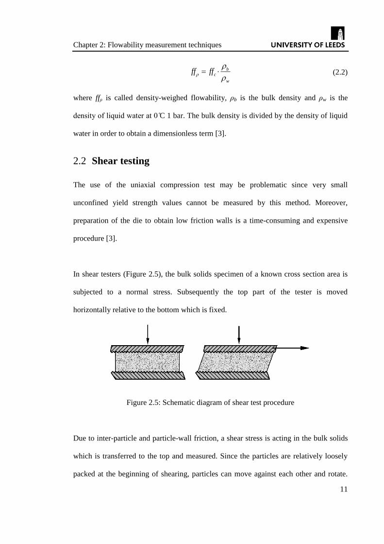
In shear testers (Figure 2.5), the bulk solids specimen of a known cross section area is
subjected to a normal stress. Subsequently the top part of the tester is moved
horizontally relative to the bottom which is fixed.
Figure 2.5: Schematic diagram of shear test procedure
Due to inter-particle and particle-wall friction, a shear stress is acting in the bulk solids
which is transferred to the top and measured. Since the particles are relatively loosely
packed at the beginning of shearing, particles can move against each other and rotate.

Chapter 2: Flowability measurement techniques
12
Inter-particle frictional forces will be small and thus the shear stress will be small at the
beginning. With increasing shear deformation the bulk solids become increasingly
compact, leading to increased frictional forces and bulk density. Finally the frictional
forces between the particles are fully mobilised which causes plastic deformation of the
bulk (known as steady-state flow). The steady-state flow transfers the bulk solids into a
well-defined, reproducible state of bulk density and strength. The process of
consolidation and shear to steady-state flow is called preshear and the shear stress at this
point is called the preshear stress, τpre. The bulk density and the shear stress at the
steady-state flow are characteristic for the applied normal stress. The preshear procedure
corresponds to the consolidation step in the uniaxial compression test, however the
required consolidation stress at preshear is precisely controlled, contrary to the uniaxial
compression test in which the total vertical stress on the specimen is assumed to be
equal to the consolidation stress. Moreover, in the case of inhomogeneous bulk solids
specimens (e.g. when local voids or region with low bulk density exist throughout the
specimen), the consolidation state of the bulk in the uniaxial compression test may not
be representative of the whole bulk, especially at low consolidation stresses. This
problem is avoided in a shear test; during preshear the inhomogeneities are compensated
by the relatively large shear deformation [3].
After preshear, the normal stress acting on the specimen is reduced to a value less than
the preshear normal stress. If the consolidated specimen is sheared (under the normal
stress σsh < σpre), it will start to flow when a sufficiently large shear stress is achieved.
At the failure of the specimen, the bulk density and shear resistance decrease which
leads to a reducing shear stress. Therefore at the start of failure, a maximum shear stress

Chapter 2: Flowability measurement techniques
13
is achieved which characterises the incipient flow. The corresponding pair values of
shear and normal stresses at the failure produce a point on shear vs. normal stress plot,
which is known as a shear point. The process of preshear to steady-state flow and shear
to failure is repeated for the same preshear stress but different normal stresses in the
shear process. This results in a number of shear points on the shear vs. normal stress
plot. A line containing all the possible shear points for a specific preshear stress is
known as the yield locus, which is shown in Figure 2.6.
Figure 2.6: Determination of yield locus in a shear test
Representation of stresses using Mohr’s stress circles 2.2.1
In order to evaluate the flowability of a bulk using a shear test, the major principal stress
and unconfined yield strength must be determined. The major principal stress can be
evaluated by drawing a Mohr’s circle of steady-state flow. This Mohr’s circle includes
the preshear point and tangent to the yield locus. Considering the fact that the centre of
the circle is on the σ-axis, the circle can be drawn (see Figure 2.7). The major principal
stress is the largest of all normal stresses acting during steady-state flow in all possible

Chapter 2: Flowability measurement techniques
14
planes of the specimen (intercept of the circle with σ-axis). This stress is comparable to
the consolidation stress of the uniaxial compression test (where σ1 is also the largest
normal stress) provided the walls are frictionless in the latter. The unconfined yield
strength cannot be measured directly with a shear test and must be determined from the
yield locus. At the failure, a normal stress and no shear stress act on the top of the
specimen, and neither normal nor shear stresses act on the lateral surface of the
specimen. The Mohr’s circle representing the failure therefore has its minor principal
stress at zero. Considering the fact that the centre of the circle is on the σ-axis, and that
the circle is tangent to the yield locus, it can be drawn as shown in Figure 2.7. The
unconfined yield stress is the intercept of this circle with σ–axis.
Figure 2.7: Mohr’s circle representation of shear test

Chapter 2: Flowability measurement techniques
15
Flowability measurements at low consolidation stresses 2.3
and tensile regimes
At low consolidation stresses as well as the region where the normal forces are tensile,
it is important to determine two parameters, cohesion and uniaxial tensile strength
(denoted as C and σT respectively). Cohesion is the value of shear stress where the yield
locus intersects with the τ-axis, i.e. where normal stress is zero. Uniaxial tensile strength
is the value of negative normal stress at which shear stress is zero, i.e. the left end of the
yield locus.
Shear testers 2.3.1
With most shear testers it is not possible to measure shear points at very small or
negative stresses because such stresses cannot easily be applied. In this case cohesion
and tensile strength can be determined only by extrapolating the yield locus towards
small and negative normal stresses [8]. Linearity is usually assumed for determination
of yield loci for very small normal stresses. Mostly yield loci are increasingly curved
towards small stresses, hence the value of the cohesion and tensile strength cannot be
determined with confidence in this way. With a few shear testers such as Schulze shear
ring tester [10] normal stresses of a few hundred Pascal can be measured. In this case,
the extrapolated value of cohesion can be close to the actual value.
Once the cohesion is determined, the tensile strength can be evaluated based on the
Warren Spring non-linear model [11], which is a predictive model for determination of

Chapter 2: Flowability measurement techniques
16
yield locus. The shear stress, τ, corresponding to the normal stress, σ, is calculated based
on the following equation,
1
n
TC
(2.3)
where C is the cohesion, σT is the tensile strength of the material and n is called the
shear index of the bulk. Shear index is a material dependent parameter and varies
between 1 and 2. It was found that shear index is not dependant on bulk density or
consolidation stress of the bulk [11].
Sevilla powder tester 2.3.2
This apparatus requires a small volume of powder and measures the uniaxial tensile
strength of the powder by applying a tensile force to a powder bed due to the pressure
drop of a percolating gas. A general schematic diagram of this tester is shown in
Figure 2.8.

Chapter 2: Flowability measurement techniques
17
Figure 2.8: Sevilla powder tester
A bulk solids specimen is located inside a vertical cylindrical vessel and is supported on
a porous plate which has pore sizes smaller than the particle size. A controlled flow of
dry gas is introduced from the bottom of the specimen through the pores. The gas flow
is increased until the powder bed is fluidised into a “freely bubbling regime”, through
which the powder bulk looses its memory of stress history [12]. Once the specimen
reaches a steady state, the gas flow is stopped and then reversed in order to apply a
compressive load. This process corresponds to the preshear stage of a shear test and
gives a reproducible starting condition for the bulk solid. In order to measure uniaxial
tensile yield stress, the gas flow is yet again reversed to an upward-directed flow that is
slowly increased to put the bed under increasing tension. The consolidation stress at the
bottom of the bed is assumed to be the total weight of the sample divided by the cross-
section area of the bed;

Chapter 2: Flowability measurement techniques
18
.
c
m g
A (2.4)
where m is the total mass of the sample, g is the gravitational acceleration and A is the
cross-section area of the bed. When the gas is passed through the particles, it exerts a
drag force on the particles, causing a pressure drop and hence a tensile stress. Close
observations reveal that fracture of the bed always starts at the bottom of the bed [12].
On increasing the gas flow rate, the tensile stress is increased until the point at which
the bed fails. Therefore the normal stress acting on the particles at the bottom of the
vessel can be calculated as follows,
.
n
m gp
A (2.5)
where Δp is pressure drop of the gas across the bed. With a constant and smooth
increase of the gas flow rate, the pressure drop is increased linearly. With free flowing
powders where there is no cohesion and yield locus originates from the origin (i.e. zero
tensile strength and cohesion values), only gravitational forces should be overcome in
order to initiate the incipient flow of the powders. The response of the pressure drop
against increasing the gas flow for free flowing powders is shown schematically in
Figure 2.9.

Chapter 2: Flowability measurement techniques
19
Figure 2.9: Schematic response of pressure drop against increasing gas flow for free
flowing powders in Sevilla powder tester
In the case of cohesive powders, inter-particle adhesive forces need to be overcome in
addition to the gravitational forces to initiate the incipient flow. Therefore a pressure
drop larger than that corresponding to the weight of the bed (i.e. the free flowing case)
is needed. The response of pressure of drop for cohesive powders is shown in
Figure 2.10.
Figure 2.10: Schematic response of pressure drop against increasing gas flow for
cohesive powders in the Sevilla powder tester
Chapter 2: Flowability measurement techniques
20
The overshoot of pressure drop beyond the bed weight per unit area when the powder
fails gives a quantitative measure of the uniaxial tensile yield stress. In order to measure
the tensile strength for different consolidation stresses, the powder is compressed by
application of a downward-directed gas flow after the steady state of the powder is
achieved (red arrows in Figure 2.8).
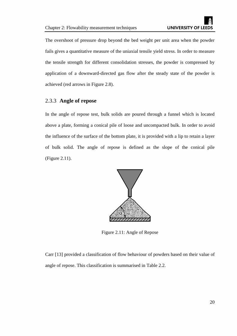
Angle of repose 2.3.3
In the angle of repose test, bulk solids are poured through a funnel which is located
above a plate, forming a conical pile of loose and uncompacted bulk. In order to avoid
the influence of the surface of the bottom plate, it is provided with a lip to retain a layer
of bulk solid. The angle of repose is defined as the slope of the conical pile
(Figure 2.11).
Figure 2.11: Angle of Repose
Carr [13] provided a classification of flow behaviour of powders based on their value of
angle of repose. This classification is summarised in Table 2.2.

Chapter 2: Flowability measurement techniques
21
Table 2.2: Classification of powder flowability based on angle of repose
Angle of repose Classification
30 Easy flowing
30 - 45 Cohesive
45 - 55 Very cohesive
55 Not flowing
Since bulk solids are falling from a height, the dynamics of the process may affect the
results. There is no control on the consolidation stresses. With cohesive powders, heaps
with a peaked tip can be observed which makes it difficult to determine the slope of the
pile.
Vibrating capillary method 2.3.4
The apparatus [14] designed for this technique is illustrated in Figure 2.12. It consists of
two tubes: a larger (in diameter) glass tube followed by a smaller (in diameter) capillary
tube. The powder sample is fed to the glass tube by a hopper on the top which is kept
full with powder during the measurements. The capillary tube is vibrated in the
horizontal direction with a frequency and amplitude-controlled vibrator. The mass of
particles discharged from the capillary for a given test is measured by a balance. The
capillary tube diameter is small enough to prevent powder flow in the absence of
vibration. The vibration amplitude is increased and the profile of mass flow rate as a
function of vibration acceleration, which is called the flowability profile, is recorded.

Chapter 2: Flowability measurement techniques
22
Hopper
Vibrator
Balance
Glass tube
Capillary tube
Figure 2.12: Schematic diagram of the apparatus for vibrating capillary method
The vibration acceleration, va, is given by Equation (2.6),
2
2av a πf (2.6)
where va is the vibration acceleration, a is the vibration amplitude and f is the vibration
frequency. A typical flowability profile is shown in Figure 2.13.

Chapter 2: Flowability measurement techniques
23
Figure 2.13: Typical flowability profile obtained by vibration capillary method [14]
As it can be seen, there is a critical vibration acceleration at which the particles start
flowing out of the capillary tube. Beyond this critical acceleration, the mass flow rate
initially increases, although eventually reaches an asymptote. Jiang et al. [14]
considered this critical vibration acceleration to be characteristic of the flow behaviour
of the bulk and compared this with the results obtained by an angle of repose test for
different grades of polymethylmethacrylate particles (see Figure 2.14).

Chapter 2: Flowability measurement techniques
24
Figure 2.14: Comparison of critical vibration acceleration in vibrating capillary method
and angle of repose for different grades of polymethylmethacrylate particles [14]
Qualitatively there is good agreement between the results obtained by the vibration
capillary method and those obtained by angle of repose test.
Ball indentation 2.3.5
Different samples of powders are pre-consolidated into a cylindrical die to various low
pressures. The die must be made of low friction materials (e.g. PTFE) in order to reduce
the effects of wall friction. The surface is then indented using a spherical indenter and
the “depth/load” cycle is recorded. The loading speed is chosen so that the indentation
process is within the quasi-static regime. From the recorded depth/load cycle, the
hardness of the consolidated bulk is determined.

Chapter 2: Flowability measurement techniques
25
Histroically indentation has been used to determine the hardness of continuum materials.
Hardness represents the resistance of a material to plastic deformation which is an
important factor in processes such as comminution, tableting, polishing and attrition
since it defines the mode and pattern of mechanical failure [15]. Hardness is affected by
anisotropy in the structure of the material, yield stress, coefficient of friction and the
geometry of the deformed region. There are a number of indentation test methods for
solid materials using different geometries of indenter such as sphere, pyramid and cone
[16]. The hardness number for these cases is calculated from the applied force, the
projected area of the impression and shape of the indenter. Spheres tend to be better
options for indentation of bulk powders, since they do not include sharp edges which
may be comparable in size with individual particle size. Moreover it is important to
avoid further consolidation of the sample during the indentation process. If the
specimen is consolidated during indentation the hardness value that is measured
afterwards may not be representative of the pre-consolidation stress of interest. The
curvature of a sphere results in a smoother transition from elastic to plastic behaviour
and allows the powder to be sheared rather than consolidated. During loading, the load
is increased at a specified rate until a desired maximum load is reached. Then the load is
decreased during unloading back to zero at the same rate. During unloading, the elastic
deformation of the sample will recover. This is schematically shown in Figure 2.15.
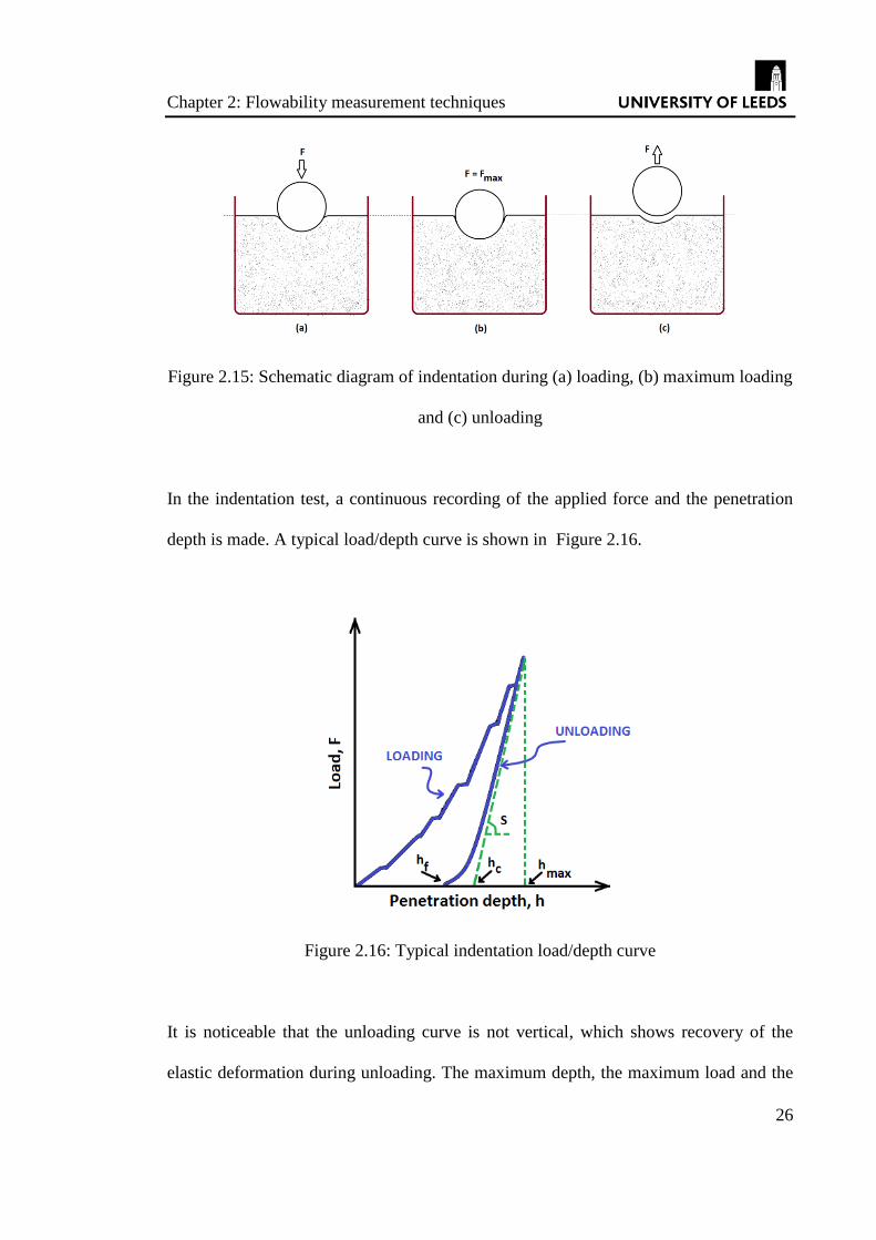
Chapter 2: Flowability measurement techniques
26
Figure 2.15: Schematic diagram of indentation during (a) loading, (b) maximum loading
and (c) unloading
In the indentation test, a continuous recording of the applied force and the penetration
depth is made. A typical load/depth curve is shown in Figure 2.16.
Figure 2.16: Typical indentation load/depth curve
It is noticeable that the unloading curve is not vertical, which shows recovery of the
elastic deformation during unloading. The maximum depth, the maximum load and the

Chapter 2: Flowability measurement techniques
27
characteristics of the unloading curve are used to calculate the hardness. Hardness is
given by the ratio of maximum indentation load to projected area of the impression,
maxFH
A (2.7)
where A is the area of the base of the spherical cap that is formed by the impression.
The relationship between a sphere and its spherical cap is given by [17],
2 2( )
2
bh rr
h
(2.8)
where r is the radius of the spherical indenter, rb is the radius of the base of the cap and
h is the height of the cap. By rearranging Equation (2.8) the projected area can be
expressed in terms of size of the indenter and depth of impression,
2 2( )bA r dh h (2.9)
where d is the diameter of the indenter and h is the depth of the impression. The depth
of the impression can be evaluated from the load/depth curve i.e. the intercept point of
unloading cycle and penetration depth axis (hf). As it can be seen from Figure 2.16 there
is a change in the height of the powder bed at the end of the unloading cycle. This
behaviour is the result of interactions between the indenter and the powder bed. For
instance, in the case of cohesive powders, the adhesive force between the indenter and
powder bed results in a slight surface lift at the end of unloading. In order to disregard
the effects of such interactions in hardness calculations, an extrapolated depth (hc),
which is representative of the initial elastic unloading, is used in Equation (2.9). hc can
be calculated by estimating the tangent to the initial elastic part of the unloading curve.
The slope of the tangential line determines the location of hc on the penetration depth
axis. In the indentation test, during formation of the local plasticity zones around the

Chapter 2: Flowability measurement techniques
28
indenter, the volume of the powder bed present in a yield condition is surrounded by an
elastically deformable region. This implies that the hardness is larger than the plastic
yield stress. This effect is called the plastic constraint [18], and is defined as the ratio of
hardness over yield stress,
H
CY
(2.10)
where C is the constraint factor, H is the hardness and Y is the yield stress. This factor is
usually greater than unity due to the increase in the local yield strength that is caused by
the elastically deforming region around the indent. In order to define the flow function it
is essential to relate hardness to yield strength. Wang et al. [5] have concluded that
indentation hardness and unconfined yield stress have a linear relationship with pre-
consolidation pressure for a number of materials. This corroborates the linear
relationship between yield stress and hardness observed for continuum solids, therefore
indicating a constant constraint factor for a given material. Figure 2.17 shows the
comparison between the indentation hardness and unconfined yield stress of Avicel.

Chapter 2: Flowability measurement techniques
29
Figure 2.17: The comparison between the indentation hardness and unconfined yield
stress as a function of pre-consolidation pressure for Avicel [5].
Hassanpour and Ghadiri [4] considered a constraint factor of 3 in order to evaluate the
yield strength of α-lactose, magnesium carbonate and salinised glass beads. These
results were compared to yield strengths measured by uniaxial compression test. A good
correlation between the indentation hardness and unconfined yield stress was found for
α-lactose and magnesium carbonate. However, the yield stresses obtained from ball
indentation and unconfined compression for salinised glass beads did not follow the
same trend. This can be ascribed to the difference in constraint factor for salinized glass
beads. Subsequently Wang et al. [5] evaluated the constraint factor for Avicel, starch
and lactose monohydrate by comparing the results of indentation and uniaxial
compression. The results are shown in Figure 2.18.
y = 0.2278x - 0.4153R2 = 0.9888
y = 1.1826x + 0.8615R2 = 0.9883
0
5
10
15
20
25
30
35
40
0
5
10
15
20
25
30
35
40
0 5 10 15 20 25 30 35
Ind
en
tati
on
Ha
rdn
es
s (k
Pa
)
Un
co
nfi
ne
d Y
ield
Str
es
s
Pre-consolidation Pressure (kPa)
Unconfined Yield Stress
Indentation Hardness

Chapter 2: Flowability measurement techniques
30
Figure 2.18: The relationship between constraint factor and pre-consolidation pressure
for Avicel, Starch and Lactose [5]
It can be concluded that the constraint factor is independent of the pre-consolidation
pressure and it is material dependant. The constraint factor for various types of
continuum solid materials has been reported in the literature. Hill [19] showed that only
for rigid-perfectly plastic materials, can the constraint factor be estimated as 3. Tabor
[16] stated that the constraint factor of 3 is only applicable for ductile metals. Johnson
[20] proposed the following relationship between the indentation hardness and yield
stress for elastic-perfectly materials, which cover a wide range of continuum solids,
2
1 ln3 3
H Ea
Y YR
(2.11)
where E is Young’s modulus, a is the radius of the impression and R is the indenter
radius. Equation (2.11) is applicable to continuous solids, and may not be valid for
discrete particulate systems. For particle assemblies there is no reported work in the
literature and the constraint factor depends on single particle properties such as particle
shape, stiffness and inter-particle friction. It was suggested by Wang et al. [5] to
0
1
2
3
4
5
6
7
0 5 10 15 20 25 30 35
Co
ns
tra
int F
ac
tor
(-)
Pre-consolidation Pressure (kPa)
Avicel Starch Lactose

Chapter 2: Flowability measurement techniques
31
investigate the effects of single particle properties on the constraint factor using DEM
analysis.
Zatloukal and Sklubalova [21] studied dynamic indentation of powders using spherical
indenter. In their work, the spherical indenter was released from a height above the
unconsolidated bulk solids and the depth of the impression was measured
experimentally. Using bulk density of the powder and the volume of impression, the
“mass of indentation” was calculated using the following equation,
i i bM V (2.12)
where Mi is the mass of indentation, ρb is the bulk density and Vi is volume of the
impression which is calculated based on the depth of impression (h) and indenter radius
(R) as follow,
213
3iV h R h (2.13)
In order to evaluate the flowability, mass flow rate, Qm, of the testing powders was
measured and correlated to the indentation mass. Sodium citrate, potassium citrate,
sorbitol, and boric acid with three size fractions in the range of 0.315 – 0.630 mm were
used in the experiments. The correlation is shown in Figure 2.19.

Chapter 2: Flowability measurement techniques
32
Figure 2.19: Linear correlation of mass flow rate and indentation mass [21]
The mass flow rate was found to have a linear correlation with indentation mass for all
the materials except sorbitol. They ascribed this exception to cohesivity of the sorbitol
powders which leads to agglomeration of the particles. A similar behaviour was found
for correlation of volume flow rate, Qv, and indentation volume, vi (Figure 2.20).
Figure 2.20: Linear correlation of volume flow rate and indentation mass [21]

Chapter 2: Flowability measurement techniques
33
It was concluded that this method of indentation can be considered as a simple method
for qualitative measurement of flowability of powders. The results were found to be
comparable to compressibility tests and Carr index. This technique needs to be
developed further by investigating more materials for a range of indentation rate. In this
method, effects of the dynamics of the indenter must also be investigated since the
indenter is dropped onto the surface of the bulk at relatively high velocities. This is
discussed in the next section.
Comparison of flowability measurement techniques 2.4
As discussed previously, in order to obtain a quantitative statement regarding
flowability of bulk solids it is essential to measure strength of the bulk for a given
consolidation state, i.e. consolidation stress (σ1) and yield strength (σc). This eliminates
the effects of powder testers on the measurements which in turn enables a comparison
of flow properties of bulk solids measured by different testing apparatuses. Schulze [3]
suggested seven criteria that a test apparatus should have in order for a powder tester to
provide quantitative and reliable results:
1. consolidation procedure with subsequent measurement of strength;
2. consolidation of the bulk solids test specimen until steady state flow has been
reached;
3. not too much difference in directions of loading and testing application i.e.
similar orientations of the major principal stresses during consolidation and
measurement of strength;

Chapter 2: Flowability measurement techniques
34
4. reproducible load application of the bulk solids specimen for consolidation (4a)
and for measuring strength (4b);
5. known average stresses in the measuring plane with possibly the most uniform
stress distribution for consolidation (5a) and for measuring strength (5b);
6. possibility for varying consolidation stresses (adjustment to application of test
results);
7. possibility for measuring increase of strength with time (time consolidation if
required for the application).
During the consolidation procedure of the uniaxial compression test there is a chance
that the consolidated bulk is non-homogenous. Moreover, friction between the solids
and cylindrical wall may result in a severe underestimation of the yield strength [8].
Nevertheless simplicity of testing procedure in uniaxial compression test is the reason
behind common usage. In contrast to the uniaxial compression test, shear testers are
more complex and the measurement are more time consuming. However, the preshear
process of a shear tester transfers the bulk solid into a fairly reproducible consolidation
state and hence the results are more reliable and reproducible compared to the uniaxial
test. With the Sevilla powder tester, the tensile strength of bulk solids is measured
which makes it applicable for cases where bulk solids are under tension instead of
compression or very low applied loads. Although bulk solids can be consolidated to a
reproducible steady state flow condition, it has been suggested by Schwedes [8] that
results from this novel technique should be compared with common tensile strength
testers such as uniaxial tensile tests in order to assess its reliability. It should also be
noted that the stress history can be removed and that the reproducible steady state flow

Chapter 2: Flowability measurement techniques
35
can be achieved if the bulk specimen can be fluidised [3]. Moreover, the consolidation
level of the reproducible state is limited; powder bed height and density defines the state
of consolidation.
Angle of repose is a very limited but simple testing technique. There is no control on the
consolidation state of the bulk solids and therefore no quantitative statement regarding
flowability of the powder can be possible. However this simple and cost-effective
technique gives a good qualitative evaluation of the flow behaviour for a range of
powders. The vibrating capillary method also provides qualitative measurement of the
powder flow, although the flow function cannot be determined since the consolidation
state of the bulk is not controllable. The ball indentation method has the potential to
become a commonly used technique due to its ability to measure flowability at low
compression stresses using very small quantities of powders. However further
developments are required regarding determination of the constraint factor. In addition
to Schulze criteria for flowability measurement apparatuses, three additional criteria can
be outlined as follows,
8. Possibility for measuring small consolidation stresses.
9. Requirement of relatively small quantities of testing powder.
10. Quantifying variation of strength across the sample.
A comparison of the potential capability of the common powder flowability
measurement techniques based on Schulze and the three additional criteria is
summarised in Table 2.3.

Chapter 2: Flowability measurement techniques
36
Table 2.3: Comparison of the common powder flowability measurement techniques based on Schulze and three additional criteria.
Criteria → 1 2 3 4 5 6 7 8 9 10 Comments
Uniaxial test ˟ ˟ ˟ ˟
Simple, but a powder is not conditioned to a reproducible
state. The sample size must be large enough to avoid
influence of the confining walls.
Biaxial test ˟ ˟ ˟ Similar to uniaxial test, but the yield locus can be measured
confidently by comparison of multiple points.
Shear test ˟ ˟ ˟
Time-consuming, but the powder is presheared to achieve a
well-defined and reproducible state. The major principal and
unconfined stresses are determined confidently.
Sevilla powder
tester ˟ ˟ ˟
Tensile strength of the bulk can be measured, but the process
is rather time-consuming. The powder can be pre-
conditioned only if it is fluidisable. Loosely compacted
samples can be used.
Angle of repose ˟ ˟ ˟ ˟ ˟ ˟ ˟ ˟ ˟ ˟
Very simple. Gives qualitative results. The unconfined yield
stress cannot be determined. The consolidation state of the
bulk is not controlled.
Vibration
capillary test ˟ ˟ ˟ ˟ ˟ ˟ ˟ ˟ ˟ ˟
Gives qualitative results. The unconfined yield stress cannot
be determined. The consolidation state of the bulk is not
controlled.
Ball
indentation ˟ ˟
Multiple tests can be performed on the same sample to
determine the distribution of strength. Very small quantities
are required. It can be performed on loosely compacted
samples but a powder is not conditioned to a reproducible
state. The unconfined yield stress is not directly measured.

Chapter 3: Distinct Element Method (DEM)
37
CHAPTER 3 Distinct Element Method (DEM)
The macroscopic bulk behaviour of powders is governed by the microscopic activity of
the individual particles in an assembly. This implies that in order to gain a better
understanding of particulate systems and their functioning, the particle interactions at
the microscopic level must be analysed. It is currently very difficult to investigate the
behaviour of individual particles within a bulk assembly experimentally. Therefore it is
helpful to model the behaviour of particles by the use of numerical simulations.
Furthermore the use of computer simulations provides a cost effective method as an
alternative to experiments since no physical material or process equipment is required,
provided that the simulation results are validated. Simulations are invaluable for cases
for which actual experiments are hazardous such as process handling of radioactive
powders. For particulate solids, the most appropriate approach for this purpose is the
use of computer simulation by the Distinct Element Method (DEM). The principal of
DEM was first introduced by Cundall and Strack [22]. In this technique, Newton’s laws
of motion is applied to describe particle motion and to describe the particle interactions
with its neighbours, contact mechanics is applied. Under the assumption that within a
time-interval the velocity of the elements is unchanged and particle interactions do not
go beyond its neighbour, the position of the elements is updated. A complete review of
the methodology of the DEM and its applications are presented elsewhere [23, 24]. In
this chapter a brief summary of the methodology is provided. A detailed review of
contact models, which have been proposed for DEM, is given since this aspect has not
been reviewed adequately in the literature. Different approaches of incorporation of
particle shape in DEM simulations are also reviewed.

Chapter 3: Distinct Element Method (DEM)
38
Time-step 3.1
Particulate systems are composed of distinct particles which displace independently
from one another and interact only at contact points [22]. Movement of a particle within
a granular flow is affected not only by the forces and torques originated from contacts
with its immediate neighbouring particles, but also by disturbance propagations from
particles far away. In order to avoid evaluation of effects of disturbance waves in DEM,
the particle displacement calculations are performed after a time-step, within which the
disturbance cannot propagate from each particle further than its immediate neighbouring
particles [22].The speed of disturbance waves is approximated by Rayleigh surface
wave propagation based on physical properties of the discrete medium. The time must
be sufficiently smaller than Rayleigh time-step in order to ensure realistic force
transmission rates in the assembly and to prevent numerical instability [25]. The
Rayleigh time-step is given by Equation (3.1).
1/2
0.1631 0.8766R
ρπR
GT
υ
(3.1)
where R is the particle radius, ρ is the density, G is the shear modulus and υ is the
Poisson’s ratio of the particle. In practice, a fraction of this maximum value is used for
the integration time-step. For dense systems with high coordination numbers (4 and
above) a typical time-step of 0.2TR has been shown to be appropriate. For lower
coordination numbers 0.4TR is more suitable [26]. Since the time-step varies with
different particle materials, for an assembly consisting of different material type
particles, the critical time-step should be the smallest among those determined for
different material properties [25].

Chapter 3: Distinct Element Method (DEM)
39
Motion calculations 3.2
Each particle within a granular flow can have two types of motion: translational and
rotational. Newton’s second law of motion is used to calculate the translational and
rotational accelerations. By integrating the accelerations over a time-step, particle
velocities and positions are updated. The rotational motion is calculated based on
Equation (3.2).
dω
I Mdt
(3.2)
where I is the moment of inertia, ω is the angular velocity, M is the resultant contact
torque acting on the particle and t is time. The translational motion is calculated based
on Equation (3.3).
g c nc
dVm F F F
dt (3.3)
where V is the translational velocity of the particle, m is the mass of the particle, Fg is
the resultant gravitational force acting on the particle and Fc and Fnc are the resultant
contact and non-contact forces between the particle and surrounding particles or walls.
Figure 3.1 is a schematic representation of these forces.

Chapter 3: Distinct Element Method (DEM)
40
Figure 3.1: Schematic representation of the forces acting on a particle
Contact and non-contact forces 3.3
Particle interactions are not just due to particle collisions and inter-particle contacts.
Particles may interact with each other while they are apart from each other, e.g. in the
case of charged particles, attractive or repulsive forces may influence the particles
motion. The following section is a brief review of common non-contact forces which
may be present in particulate systems.
Van der Waals forces 3.3.1
Van der Waals force is a result of dipole interactions between molecules. Different
electronic configurations of molecules give them a dipolar character which may result in
attractions. Van der Waals force operates both in gaseous and liquid environments,
although it is substantially reduced in liquid environments [27]. Hamaker [28]
calculated the interaction force between a sphere and a semi-infinite body, by
summarising all the possible individual molecular interactions, as follows [29],

Chapter 3: Distinct Element Method (DEM)
41
212
H
van
A RF
d (3.4)
where AH is the Hamaker coefficient which is a material property related to the
molecular properties of the particle with radius of R, and d is the separation distance
between the two bodies. The van der Waals forces become noticeable when particles
can come sufficiently close together, that is at separation distances of the order of the
size of a molecule (i.e. 0.2 to 1nm). Moreover, the magnitude of van der Waals forces
becomes negligible compared with that of the gravitational force when the particle size
exceeds a few microns. This is due to the fact that the gravitational force is proportional
to the cube of the particle diameter, but the van der Waals force is proportional to the
diameter. Once the particles are in contact, the overall van der Waals attraction is
increased significantly due to increase in the contact area. This situation is enhanced
when plastic deformation takes place [27].
Liquid bridges 3.3.2
In humid systems (with a relative humidity of > 60%) capillary condensation of the
fluid in the gap between the particles in close contact may take place resulting in an
attraction. The maximum attraction is achieved for two smooth spherical particles if the
liquid covers the particle surfaces completely. For this case, the liquid bridge attraction
force, FLB, can be calculated as follow [27],
2LBF πγR (3.5)
where γ is the surface tension of the liquid and R is the radius of the two particles.

Chapter 3: Distinct Element Method (DEM)
42
Electrostatics 3.3.3
Electrostatic forces can form as a result of tribo-electric charging or formation of a
potential difference between particles. In the latter case, charged particles attract
adjacent uncharged particles due to their own image charge. The attraction force can be
evaluated by the classical Coulomb equation [27],
2
2 2
_ 2
0
1
16t elec
dQ
R dF
πε d
(3.6)
where Q and R are the charge and radius of the charged particle, d is the separation
distance between the two bodies, and ε0 is the permittivity of the vacuum. In the former
case i.e. potential difference, particles with a different work-function can form a
potential difference when they are brought together. This results in an attraction force
which can be calculated as follows [27],
20
_ ΔV elec
πε RF V
d (3.7)
where ΔV is the potential difference formed by the contact. It should be noted that in
humid environments the Coulomb attraction is reduced to zero due to the fact that
particle surfaces are covered by the liquid, which mostly is a conductor resulting in
charge leakage and discharging.
Contact Force Models 3.4
In order to consider particle interactions in the calculations, the resulting forces from
particle collisions and contacts are modelled. There exist a number of force models
which mostly allow particles to have deformation. The deformation is modelled as an
overlap between particles. In the general case of an assembly of many particles, the

Chapter 3: Distinct Element Method (DEM)
43
contact force model is applied at each contact and the vectorial sum of these contact
forces is determined to yield the resultant contact force acting on that particle [22].
There has been extensive work in the literature in order to develop accurate and/or
computationally efficient models based on theories of contact mechanics to be
employed in DEM simulations. Mostly these models are developed for spherical
contacts based on Hertz theory. Following is a brief review of the most commonly used
contact models. Four categories are considered for contact models: elastic, elasto-plastic,
elastic-adhesive and elasto-plastic-adhesive models. For each category normal and
tangential contact models are described.
Elastic contacts 3.4.1
3.4.1.1 Linear spring contact model
In this simple model [22] the contact force between two perfectly elastic spheres is
resolved into normal and shear components with respect to the contact plane,
n sF F F (3.8)
where F is the contact force, and Fn and Fs are the normal and shear components of the
contact force. The normal contact force is calculated from the overlap of the particles in
contact,
n n nF k α (3.9)
where αn is the normal overlap and kn is the normal stiffness at the contact which can be
calculated as follow,
1 2
1 2
n nn
n n
k kk
k k
(3.10)

Chapter 3: Distinct Element Method (DEM)
44
where 1
nk and 2
nk are the normal stiffness for the particles in contact. Figure 3.2 shows a
schematic force-overlap response of linear-spring model.
α
f
kn α
Figure 3.2: Schematic of force-overlap response of linear-spring model
The increment of shear force in this model is calculated from,
Δ Δs s sF k α (3.11)
where Δαs is the increment of shear displacement of the contact and ks is the shear
contact stiffness which can be calculated as follow,
1 2
1 2
s ss
s s
k kk
k k
(3.12)
where 1
sk and 2
sk are the shear stiffness for the particles in contact. The total shear force
is found by summing up the previous shear force with the increment of shear force,
' Δs s sF F F (3.13)
where '
sF is the previous shear force [22].

Chapter 3: Distinct Element Method (DEM)
45
3.4.1.2 Hertz normal contact model
Based on this model [30], the normal contact force between two perfectly-elastic
spheres in contact is given by [31],
1/2* * 3/24
3nF E R α (3.14)
where E* and R
* are the equivalent Young’s modulus and radius which are given by
Equations (3.15) and (3.16), respectively, and α is the normal overlap.
12 2
* 1 2
1 2
1 1υ υE
E E
(3.15)
E1 and E2 are Young’s moduli of the particles in contacts, and υ1 and υ2 are Poisson’s
ratios of the particles in contact.
1
*
1 2
1 1R
R R
(3.16)
R1 and R2 are the radii of the particles in contact.
3.4.1.3 Mindlin and Deresiewicz’s tangential contact model
Mindlin and Deresiewicz [32] developed a tangential model for perfectly elastic
contacts. Due to tangential slip at the contact, the tangential force-displacement
relationship depends on the loading history and on the rate of change of the normal and
tangential force. Following is a description of the model for cases where the normal
displacement does not change (i.e. the radius of the contact area is constant) through the
change of tangential force:
The tangential force is calculated using the following general equation,

Chapter 3: Distinct Element Method (DEM)
46
0 0t t t t tf f k α α (3.17)
where ft0 is the previous tangential force, αt – αt0 is the change in tangential
displacement (the same as Δαs in the linear-spring model) and kt is the tangential
stiffness. Initially, when the tangential displacement starts increasing, the tangential
stiffness is calculated based on Equation (3.18),
1/3
10 1 t
t t
n
fk k
μf
(3.18)
where μ is the coefficient of sliding friction and kt0 and ft1 are given by Equations (3.19)
and (3.21), respectively.
1/2* * 1/2
0 8t nk G R α (3.19)
where G*
is the equivalent contact shear modulus given by Equation (3.20),
12 2
* 1 2
1 2
1 1υ υG
G G
(3.20)
where G1 and G2 are the shear moduli of the particles in contact.
1 0
2
3t t tf k α (3.21)
The contact starts sliding (macro-slip) once the tangential force reaches Coulomb’s limit
of friction given by Equation (3.22).
t nf μ f (3.22)
Before the macro-slip occurs, there are regions in the contact area where the shear stress
exceed the Coulomb’s limit [33]. Therefore, small local tangential displacement occurs
while the remainder of the contact area is not relatively displaced. This phenomenon is
known as micro-slip. If the contact is unloaded in the tangential direction, the unloading
path on the force-displacement curve would be different to that of the loading curve due

Chapter 3: Distinct Element Method (DEM)
47
to the micro-slip. Mindlin and Deresiewicz [32] considered a hysteretic behaviour to
account for the micro-slip, by which the unloading tangential stiffness is given by,
1/3
10 1
2
TP
t tt t
n
f fk k
μf
(3.23)
where TP
tf is the tangential force at the point when the contact is unloaded tangentially
(turning point). The unloading curve follows Equation (3.23) up to TP
tf , where the
history of the turning point becomes insignificant [32]. If the contact is unloaded further,
the tangential stiffness is the same as the initial stiffness which is given by Equation
(3.18). In the case of subsequent turning points, the tangential stiffness is evaluated
using the following equation,
1/3
10 1
2
TTP
t tt t
n
f fk k
μf
(3.24)
where TTP
tf is the tangential force at the second turning point. Figure 3.3 shows a
schematic tangential force-displacement response of Mindlin and Deresiewicz’s model.

Chapter 3: Distinct Element Method (DEM)
48
αt
ft
TP
tf
TTP
tf
TP
tf
nμf
nμf
1/3
1
0 1 t
t t
n
fk k
μf
1/3
1
0 1TP
t t
t t
n
f fk k
μf
1/3
1
0 1TTP
t t
t t
n
f fk k
μf
Figure 3.3: Schematic tangential force-overlap response of Mindlin and Deresiewicz’s
model
In cases where both the tangential and normal displacements vary, the tangential force is
evaluated by assuming that the change in the normal displacement is not significant.
Mindlin and Deresiewicz [32] considered a “simple loading history” which enables
solving the problem by superposition of the effects of change in tangential and normal
displacements. This simple loading history defines a linear tangential stiffness which
facilitates the tangential force to be adopted for the response corresponding to the new
normal force. It is best to make use of illustrations to describe this complicated model.
Figure 3.4 shows the tangential force-displacement response of the case where both
normal and tangential displacements increase.

Chapter 3: Distinct Element Method (DEM)
49
αt
ft
nμf
1/3
1
0
1
1 t
t t
n
fk k
μf
1/3
1
0
2
1 t
t t
n
fk k
μf
A
B
Δ nμ f1 2
2 1Δ
n n
n n n
f f
f f f
Figure 3.4: Schematic tangential force-overlap response of Mindlin and Deresiewicz’s
model for the case where both normal and tangential displacements increase
In Figure 3.4, initially the tangential force increases while the normal force is assumed
to be constant with a value of fn1. For this part of the loading, the tangential stiffness is
calculated based on Equation (3.18). At point A, the normal force is increased by Δ nf to
the value fn2. Based on the simple loading history that Mindlin and Deresiewicz [32]
proposed, the contact is loaded with a linear tangential stiffness so that the response
meets the response of a contact which was loaded initially with a constant normal force
of fn2 at point B which corresponds to a tangential force of Δ nμ f . For unloading and
reloading cases near turning points, the response of the model is treated in the same
manner.
3.4.1.4 Mindlin’s no-slip tangential contact model
Mindlin [34] proposed a tangential model for perfectly elastic contacts by neglecting the
effects of micro-slip. The hysteretic behaviour which was considered for Mindlin and
Deresiewicz’s model [32] is not present in this model. The loading and unloading path
of the tangential force is the same and the tangential stiffness is given by,

Chapter 3: Distinct Element Method (DEM)
50
1/2* * 1/28t nk G R α (3.25)
Di Renzo and Di Maio [35] simulated oblique impact of a particle to a flat wall at
different impact angles using the linear spring, Mindlin’s no-slip and Mindlin and
Deresiewicz’s models. The comparison of the results to the experimental findings of
Kharaz et al. [36] are shown in Figure 3.5.
Figure 3.5: Comparison of linear-spring, Mindlin’s no-slip and Mindlin and
Deresiewicz’s models with the experimental data for oblique impact of a particle at
different impact angles [35]
Figure 3.5 shows a very good agreement of the three models with the experimental
results, except for small impact angles. The linear model surprisingly produced better
results compared to Mindlin’s no-slip model.

Chapter 3: Distinct Element Method (DEM)
51
3.4.1.5 Di Renzo and Di Maio’s no-slip tangential contact model
Di Renzo and Di Maio [37] proposed a modification to Mindlin’s no-slip tangential
model [34] so that the macro-slip occurs at the same tangential overlap that Mindlin and
Deresiewicz[32] predicted. The tangential stiffness is given by Equation (3.26),
1/2* * 1/22 16
3 3t tM nk k G R α (3.26)
where ktM is the tangential stiffness of Mindlin’s no-slip model. This model has the
advantage of being simple and computationally cost-effective (similar to Mindlin’s no-
slip model). Figure 3.6 shows comparison of Mindlin’s no-slip [34], Di Renzo and Di
Maio’s no-slip [37] and first loading of Mindlin and Deresiewicz’s [32] tangential
models.
αt
ft
nμf
Mindlin no-slip
Mindlin and
Deresiewicz
Di Renzo and
Di Maio
Figure 3.6: Comparison of Mindlin’s no-slip, Di Renzo and Di Maio’s no-slip and first
loading of Mindlin and Deresiewicz’s tangential models.
It was analytically shown that for small impact angles the model of Di Renzo and Di
Maio provides a better match to Mindlin and Deresiewicz’s model in cases where both
normal and tangential displacements occur compared to the no-slip model of Mindlin
[37]. Di Renzo and Di Maio [35, 37] compared the tangential force response of Hertz-

Chapter 3: Distinct Element Method (DEM)
52
Mindlin’s no-slip (HM), Hertz-Mindlin and Deresiewicz’s (HMD) and Hertz-Di Renzo
and Di Maio’s (HDD) for a particle impacting on a flat wall at different impact angles.
Figure 3.7 shows the tangential force-displacement of the three models at two different
impact angles.
Figure 3.7: Tangential force-displacement of Hertz-Mindlin’s no-slip (HM), Hertz-
Mindlin and Deresiewicz’s (HMD) and Hertz-Di Renzo and Di Maio’s (HDD) models
at two different impact angles [37]
As it can be seen, HDD model shows a better agreement with HMD compared to HM
model. The tangential force-displacement response of HDD model becomes closer to
that of HMD model at higher impact angles.

Chapter 3: Distinct Element Method (DEM)
53
Elasto-plastic contacts 3.4.2
3.4.2.1 Thornton’s elasto-plastic normal contact model
In this model [38] the contact force follows Hertz elastic model until it reaches the yield
force after which the contact is deformed plastically. The yield force is given by
Equation (3.27),
2
2
3 *3
*6y y
π RF p
E (3.27)
where py is the yield pressure of the contact. Plastic deformation in this model is
governed by a constant stiffness of πpyR* based on the assumptions that the contact
pressure does not increase further than the yield pressure and that the pressure
distribution over the contact area is Hertzian [31]. The contact force during plastic
deformation can be calculated using the following equation,
*
n y y yF F πp R α α (3.28)
where αy is the overlap at which the contact yields and is given by,
2
2 *2
*4y y
π Rα p
E (3.29)
If plastic deformation occurs during the loading stage, the contact curvature during
unloading is less than that of the elastic unloading curvature due to permanent
deformation of the contact surfaces. During unloading, the force-displacement
behaviour is assumed to be elastic and is provided by the Hertz equations but with a
curvature of *1/ pR corresponding to the point of maximum compression. This curvature
can be evaluated based on the maximum force the contact experiences during the plastic
loading, Fmax, as given by Equation (3.30),

Chapter 3: Distinct Element Method (DEM)
54
3/2*
max*
max
24
3 2
y
p
y
F FER
F πp
(3.30)
Since the unloading is considered to be purely elastic based on Hertz theory [30], the
equation for the unloading is given by,
1/2 3/2
* *4
3n pF E R α α (3.31)
where αp is the permanent plastic deformation given by Equation (3.32),
*
max *1p
p
Rα α
R
(3.32)
where αmax is the maximum overlap during plastic loading. Figure 3.8 is a schematic
force-overlap response of Thornton’s model.
α
f
Fmax
Fy
αy αp αmax
Figure 3.8: Schematic force-overlap response of Thornton’s elasto-plastic model
Finite Element Analysis (FEA) of elasto-plastic contacts showed that when the normal
stress exceeded the yield pressure, the force-overlap curves were not straight lines [39].
This is shown in Figure 3.9.

Chapter 3: Distinct Element Method (DEM)
55
Figure 3.9: FEA force-overlap response of an elasto-plastic contact obtained by Vu-
Quoc and Zhang [39]. The contact is unloaded at three different maximum overlaps.
In Figure 3.9 a red line is drawn from the yield point to the maximum loading overlap in
order to show that the response in the plastic regime is not linear as assumed by
Thornton [31]. It is noteworthy however, that the non-linear response in the plastic
regime does not significantly deviate from the linear extrapolation. This shows that the
assumptions made by Thornton for a linear plastic stiffness may be adequate.
Vu-Quoc and Zhang [39] compared the pressure distribution over the contact area
obtained by FEA to that of Hertz for different maximum overlaps (see Figure 3.10).

Chapter 3: Distinct Element Method (DEM)
56
Figure 3.10: Pressure distribution over half of the contact area obtained by FEA and
Hertzian pressure distribution for three different maximum loading force
The shape of the distribution in the plastic regime obtained by FEA is in agreement with
Thornton’s assumption where a Hertzian pressure distribution with a cut-off
corresponding to the limiting contact pressure was assumed [31]. However, as it was
denoted by Vu-Quoc and Zhang [39], the maximum contact pressure in Thornton’s
model is larger than the one obtained by the FEA. As a result, the radius of the contact
area obtained from FEA is less than the one predicted by Thornton for the same normal
force.
3.4.2.2 Vu-Quoc and Zhang’s elasto-plastic normal contact model
Vu-Quoc and Zhang [39] proposed a non-linear elasto-plastic model for spheres in
collision, based on additive decomposition of the radius of the contact area into an
elastic part and a plastic part. In this model the contact follows Hertz elastic curve up to

Chapter 3: Distinct Element Method (DEM)
57
a yield point (similar to Thornton’s model). The yield force for two identical spheres in
contact is given by Equation (3.33),
2
3 2 23
2
1
6y y y
π R υF A υ p
E
(3.33)
where Ay(υ) is a scalar depending only on Poisson’s ratio. Vu-Quoc and Zhang [39] did
not define this scalar, however Vu-Quoc et al. [40] provided two example values; for
Poisson’s ratio of 0.3, Ay(υ) = 1.61 and for υ = 0.4, Ay(υ) = 1.74. Comparing Equations
(3.33) and (3.27), it can be observed that the yield force calculated in Thornton’s model
[38] is very similar to that of Vu-Quoc and Zhang’s. Vu-Quoc and Zhang [39] derived
a very complex equation for evaluation of contact force during plastic deformation
which is given by,
1/3
21/23 11 1
1 04
n y n c n y n
a a
R υF F F K F F Rα
C E C
(3.34)
where Ca and Kc are fitted parameters obtained from FEA results. Ca in fact defines the
relationship between the plastic component of the contact radius and the contact force.
Kc defines the permanent deformation relative to the particle radius. Equation (3.34) is a
very complex equation for which there is no straight-forward solution. Vu-Quoc and
Zhang [39] suggested solving this equation by Newton-Raphson iterative method
provided a tolerance value. They showed that for a number of cases within a reasonable
tolerance, the equation can be solved after a few iterations [39]. For calculation of the
unloading contact force, Hertzian behaviour is considered where a corrected contact
curvature, *
pR , is considered similar to Thornton’s model. *
pR is given by following
equation.

Chapter 3: Distinct Element Method (DEM)
58
* *1p c yR K F F R (3.35)
Vu-Quoc and Zhang [39] compared the force-overlap response of the FEA results and
that of their model to the response of Thornton’s model which is shown in Figure 3.11.
Figure 3.11: Force-overlap response of FEA, Vu-Quoc and Zhang’s and Thornton’s
models [39]
The elastic part of the response in all models overlaps, since they all considered
Hertzian behaviour for this region. During the plastic deformation, however, the
response of Thornton’s model shows significantly lower plastic stiffness compared to
the responses of Vu-Quoc and Zhang’s model and FEA. The agreement between the
FEA results and those of Vu-Quoc and Zhang’s model is expected since the parameters
of the model are evaluated from FEA simulations. Following is a critique of this model:

Chapter 3: Distinct Element Method (DEM)
59
For the plastic regime, the contact radius, aep, is considered to be addition of the elastic
Hertzian contact radius, ae, and a plastic contact radius, ap. Figure 3.12 shows the plastic
contact radius, ap, as a function of normal contact force, where ap is calculated by
subtracting ae from the results of FEA [39].
Figure 3.12: Plastic contact radius as a function of normal contact force during loading
and unloading of a contact [39]
Vu-Quoc and Zhang concluded from Figure 3.12 that the plastic contact radius is a
linear function of normal contact force during plastic contact loading. The parameter Ca
is in fact the slope of this linear line. The unloading part of the response in Figure 3.12
surprisingly shows dependency of ap with contact unloading force. In fact, the plastic
contact radius reduces to almost half of its maximum value during unloading. Therefore
the contact unloading is not purely elastic. Vu-Quoc and Zhang claimed that FEA
simulations were performed for elastic-perfectly plastic materials, which contradicts the
unloading behaviour of Figure 3.12. The full description of FEA simulations is

Chapter 3: Distinct Element Method (DEM)
60
necessary to verify this. In general, the complexity of the non-linear equation for
evaluation of plastic contact force as well as the fact that FEA simulations must be
performed previously in order to get the input parameters of this model, result in
increasing the computational cost extensively.
3.4.2.3 Walton and Braun normal elasto-plastic model
Walton and Braun [41] proposed a simple linear model for elasto-plastic contacts. For
contact loading, the normal force is given by,
n pF k α (3.36)
where kp is the plastic stiffness. The unloading force is calculated based on Equation
(3.37),
0n eF k α α (3.37)
where ke is the elastic stiffness and α0 is the permanent contact deformation. Figure 3.13
shows a schematic of the force-overlap response of this model.
α
f
kp α
ke α
α0
Figure 3.13: Schematic force-overlap response of Walton and Braun’s [41] model with
constant coefficient of restitution

Chapter 3: Distinct Element Method (DEM)
61
Since the slopes kp and ke are constant, the coefficient of restitution of this model is
independent of impact velocity ( e = (kp/ke)1/2
). This is not in agreement with
experimental and numerical analyses in the literature [42]. In order to account for
dependency of coefficient of restitution on impact velocity, Walton and Braun [41]
suggested an elastic unloading stiffness which increased linearly with the maximum
loading force with a slope S. The equation for the elastic stiffness is given by,
max.e pk k S F (3.38)
where Fmax is the maximum loading force. The parameter S was not given any physical
definition. However, one can specify S on the basis of giving the best fit of the
unloading line of the model to the Hertz elastic equation. Figure 3.14 shows a schematic
force-overlap response of Walton and Braun’s [41] model with varying coefficient of
restitution.
α
f
kp α
ke α
ke = kp + S.Fmax
α0
Figure 3.14: Schematic force-overlap response of Walton and Braun’s [41] model with
varying coefficient of restitution
A more comprehensive model may consider the contact to be elastically deforming
(with stiffness ke) initially up to a yield limit above which the contact deforms

Chapter 3: Distinct Element Method (DEM)
62
plastically, similar to the models of Thornton, and Vu-Quoc and Zhang. However, in
real contacts, the presence of asperities always leads to plastic deformation from the
beginning of loading. Moreover, for typical ratios of Young’s modulus to yield stress of
elasto-plastic materials, the initial elastic deformation is negligible: considering
Thornton’s model, the single particle strain at which the contact yield occurs can be
calculated by dividing the yielding overlap, which is given by Equation (3.29), by 2R*.
Hence the yield strain, γy, is given by,
22 2
* * 2
1
2 8 8
y y
y
α pπ πγ
R E C
(3.39)
where C is the ratio of effective Young’s modulus to contact yield pressure which
typically has a minimum value of about 50 and can range up to a few 1000 for materials
with notable plastic component. Figure 3.15 shows the yield strain (percentage) as a
function of C which ranges from 50 to 300.
Figure 3.15: Yield strain as a function of C
0.00
0.01
0.02
0.03
0.04
0.05
0.06
0 30 60 90 120 150 180 210 240 270 300
Yie
ld s
tra
in (
%)
C (-)

Chapter 3: Distinct Element Method (DEM)
63
It can be concluded that generally the yield strain is negligible; therefore excluding an
initial elastic deformation for the contact model would not prevent the model from
capturing the realistic behaviour.
3.4.2.4 Tangential force in elasto-plastic contacts
Vu-Quoc et al. [43] considered the model of Mindlin and Deresiewicz [32] for FEA
modelling of elasto-plastic contacts. The normal force was evaluated in a similar
manner to [39] (see Section 3.4.2.2). It was shown that when the normal force is
constant while the tangential displacement is increased, the tangential force-
displacement curve becomes stiffer, in contrast to the case where both normal and
tangential displacements are increased [43]. It was concluded that a tangential model for
elasto-plastic contacts must facilitate approximation of tangential stiffening and
softening under constant and varying normal force, respectively. In contrast to the
analysis of Vu-Quoc et al. [43], Ning [44] assumed that Mindlin’s no-slip solution
remains valid for elasto-plastic contacts. Simulation of oblique impact of elasto-plastic
particles using the model of Thornton [38] for normal force calculations and Equation
(3.25) for evaluation of tangential force showed that that the tangential force-time
curves were affected by plastic deformation at low impact angles, however for other
impact angles the pattern of evolution was similar to that under elastic deformation [44].
Elastic-adhesive contacts 3.4.3
3.4.3.1 JKR elastic-adhesion normal contact model
JKR theory [45] assumes that the attractive forces are confined within the area of
contact and are zero outside. In other words, the attractive inter-particle forces are of

Chapter 3: Distinct Element Method (DEM)
64
infinitely short range. JKR model extends the Hertz model to two elastic-adhesive
spheres by using an energy balance approach. The contact area predicted by the JKR
model is larger than that by Hertz. Consequently there is an outer annulus in the contact
area which experiences a tensile stress. This annulus surrounds an inner circular region
over which a Hertzian compressive distribution acts [46].
Figure 3.16 shows schematically the force-overlap response of JKR model.
α
f
α0
αf
fc
8/9 fc5/9 fc
Figure 3.16: Schematic force-overlap response of JKR model
When two spheres come into contact, the normal force between them will immediately
drop to a certain value (8/9 fc, where fc is the pull-off force [31]) due to van der Waals
attractive forces. The velocity of the spheres are then reduced gradually and part of the
initial kinetic energy is radiated into the substrates as elastic waves. The particle
velocity will reduce to zero at a point where the contact force reaches a maximum value
and the loading stage is complete. In the recovery stage, the stored elastic energy is
released and is converted into kinetic energy which causes the spheres to move in the

Chapter 3: Distinct Element Method (DEM)
65
opposite direction. All the work done during the loading stage has been recovered when
the contact overlap becomes zero. However at this point the spheres remain adhered to
each other and further work (known as work of adhesion) is required to separate the
surfaces. The contact breaks at a negative overlap, αf, with the contact force being 5/9 fc
[44]. Pull-off force, fc, is the maximum tensile force the contact experiences and is given
by [45],
*3Γ
2cf πR (3.40)
where Г is the interface energy. The governing equation for the force-overlap relation is
given by [20],
* 3
1/2* 3
*
48 Γ
3n
E aF π E a
R (3.41)
where a is the contact radius. The overlap can be evaluated by Equation (3.42) [20],
1/22
* *
2 Γa π aα
R E
(3.42)
3.4.3.2 Savkoor and Briggs’ tangential model for elastic-adhesive contacts
Savkoor and Briggs [47] extended the JKR model to account for the effects of varying
tangential displacement. The tangential stress distribution over the contact area was
considered to be the no-slip solution of Mindlin [34] (see Section 3.4.1.4), therefore the
tangential force-displacement can be evaluated by Equation (3.25). By applying an
energy balance, Savkoor and Briggs [47] showed that the contact radius will be affected
by the tangential displacement. The contact radius is given by Equation (3.43),
2 **3 2
* *
32 4 4
4 4
tn c n c c
F ERa F F F F F
E G
(3.43)

Chapter 3: Distinct Element Method (DEM)
66
where Fn is the normal contact force, Fc is the JKR pull-off (see Equation (3.40)) and Ft
is the tangential force evaluated by Equation (3.25). The contact radius according to the
JKR model is given by [45],
*
3 2
*
32 4 4
4n c n c c
Ra F F F F F
E (3.44)
Comparing Equations (3.43) and (3.44) shows that the contact force is indeed reduced
by increasing the tangential force. Savkoor and Briggs [47] suggested that this reduction
corresponds to “peeling” mechanism which continues until a critical value of the
tangential force, Ftc, is reached,
*
2
*
16tc n c c
GF F F F
E (3.45)
If the tangential displacement increases beyond the point corresponding to Ftc, the
peeling process is complete and the contact area would immediately reduce to the
Hertzian contact area which is given by,
*
3
*
3
4n
Ra F
E (3.46)
3.4.3.3 Thornton and Yin’s tangential model for elastic-adhesive contacts
Thornton and Yin [46] proposed a modified version of Savkoor and Briggs’ [47] model.
Thornton and Yin [46] showed that the critical tangential force which provided peeling
failure (Equation (3.45)) could be larger than the tangential force required to cause
sliding. It was concluded that the contacting surfaces must “peel” before contact sliding
occurs. In order to account for this, a smooth transition from peeling to sliding was
proposed. The tangential and normal forces of this model follow Savkoor and Briggs

Chapter 3: Distinct Element Method (DEM)
67
[47] model up to the critical tangential force, Ftc. With further tangential displacement,
the tangential force is given by,
3/2
2 1 1t n c
s
αF μ F F
α
(3.47)
where αs is given by,
*
23
16
n cs
F Fα μ
G a
(3.48)
The sliding criteria which is followed by peeling failure is given by,
2t n cF μ F F (3.49)
In order to illustrate the transition of peeling to sliding, tangential force-overlap
responses of an adhesive-elastic contact with two different constant normal forces are
shown in Figure 3.17.
Figure 3.17: Tangential force-overlap response of Thornton and Yin’s model for two
different constant normal forces [46]

Chapter 3: Distinct Element Method (DEM)
68
Figure 3.17(a) shows the smooth transition after peeling failure at point Ftc to the sliding
point. In Figure 3.17(b) at the point where peeling is complete, the tangential force is
larger than the critical sliding force, hence the force is reduced to μ(Fn + 2Fc). Thornton
and Ning [46] compared their model with the results of friction measurements reported
by Briscoe and Kremnitzer [48] . The comparison is shown in Figure 3.18.
Figure 3.18: Comparison of the experimental work of Briscoe and Kremnitzer with the
model of Thornton and Yin [46]
The model can therefore capture the experimental behaviour accurately.
3.4.3.4 DMT elastic-adhesive normal contact model
DMT model [49] assumes that the attractive forces all lie outside the contact zone. The
attraction forces are also assumed not to change the deformed profile from that of Hertz.
However outside the contact area a tensile stress is assumed to have presence which
decreases with surface separation. At the point of contact prior to any deformation, the
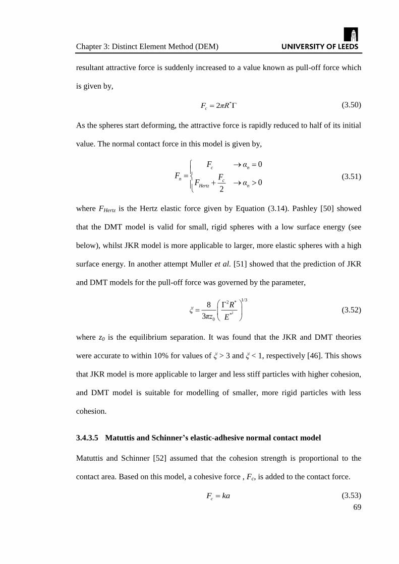
Chapter 3: Distinct Element Method (DEM)
69
resultant attractive force is suddenly increased to a value known as pull-off force which
is given by,
*2 ΓcF πR (3.50)
As the spheres start deforming, the attractive force is rapidly reduced to half of its initial
value. The normal contact force in this model is given by,
0
02
c n
n cHertz n
F α
F FF α
(3.51)
where FHertz is the Hertz elastic force given by Equation (3.14). Pashley [50] showed
that the DMT model is valid for small, rigid spheres with a low surface energy (see
below), whilst JKR model is more applicable to larger, more elastic spheres with a high
surface energy. In another attempt Muller et al. [51] showed that the prediction of JKR
and DMT models for the pull-off force was governed by the parameter,
2
1/32 *
*0
8 Γ
3
Rξ
πz E
(3.52)
where z0 is the equilibrium separation. It was found that the JKR and DMT theories
were accurate to within 10% for values of ξ > 3 and ξ < 1, respectively [46]. This shows
that JKR model is more applicable to larger and less stiff particles with higher cohesion,
and DMT model is suitable for modelling of smaller, more rigid particles with less
cohesion.
3.4.3.5 Matuttis and Schinner’s elastic-adhesive normal contact model
Matuttis and Schinner [52] assumed that the cohesion strength is proportional to the
contact area. Based on this model, a cohesive force , Fc, is added to the contact force.
cF ka (3.53)

Chapter 3: Distinct Element Method (DEM)
70
where a is the contact area and k is a constant with the units of J.m-3
. DEM-Solutions
[26] named this constant, cohesion energy density. The physical meaning of this
parameter has not been given by Matuttis and Schinner [52]. Hassanpour et al. [53]
derived an equation for the cohesion energy density based on the JKR interfacial energy
by equating the tensile work of Matuttis and Schinner [52] model to the cohesion work
of JKR [45] model,
2 1/3*
*
Γ0.75
Ek
R
(3.54)
where Г is the JKR interfacial energy. Figure 3.19 compares the force-overlap responses
of the models of Hassanpour et al. [53] and JKR [45].
Figure 3.19: Comparison of force-overlap response of JKR and Hassanpour et al.
models [53]
As it can be seen, the contact force in the compressive side deviates extensively from
that of JKR. It must be noted that Hassanpour et al. [53] used this model to simulate a

Chapter 3: Distinct Element Method (DEM)
71
high shear granulation process. The dynamics of such systems results in collision-
dominant behaviour, in which the influence of contact stiffness is insignificant (see e.g.
[54]).
Elasto-plastic and adhesive contacts 3.4.4
3.4.4.1 Thornton and Ning’s elasto-plastic and adhesive normal contact model
Thornton and Ning [31] followed the same approach as Thornton [38] used for elastic-
adhesive contacts, to develop a model for elasto-plastic and adhesive contacts. The
pressure distribution over the contact area was considered to be the same as that of JKR
model with a cut-off corresponding to the limiting contact pressure. Based on this
assumption, an equation was derived for the contact yield pressure which is given by
Equation (3.55),
1/2* *
*
2 2Γy
y
y
E a Ep
πR πa
(3.55)
where ay is the contact radius at which the plastic yield occurs. During the plastic
deformation, the contact deforms linearly with a stiffness which is given by Equation
(3.56),
3/2* *
3/2
3 2 /
3 /
y y c
n
c
πR σ E a a ak
a a
(3.56)
where ac is the contact radius at the pull-off force given by Equation (3.57) and a is the
JKR contact radius from which the normal overlap can be evaluated (see Equation
(3.42)).
1/3*
*
3
4
cec
R fa
E
(3.57)

Chapter 3: Distinct Element Method (DEM)
72
where fce is the JKR pull-off force given by Equation (3.40). If plastic deformation
occurs during the loading stage, the contact curvature during unloading is less than that
of elastic unloading curvature due to permanent deformation of the contact surfaces.
During unloading the force-displacement behaviour is assumed to be elastic-adhesive
and is provided by the JKR equations, but with a curvature of *
pR corresponding to the
point of maximum compression. This curvature can be evaluated based on the
maximum force the contact experiences during the plastic loading, Fmax, as given by
Equation (3.58),
* *
* max
*
max max4p
ce
R FR
F F F
(3.58)
where *
maxF is the equivalent JKR force of Fmax. The plastic pull-off force (i.e. the
maximum tensile force the contact experiences after plastic deformation) of this model
is given by Equation (3.59),
*3
Γ2
cp pF π R (3.59)
Figure 3.20 shows a schematic force-overlap response of Thornton and Ning’s model.
α
f
Fmax
Fy
αfp
αmaxαy
Fce
Fcp
5/9 Fcp
8/9 Fcp
αc0αf
Figure 3.20: Schematic force-overlap response of Thornton and Ning’s model

Chapter 3: Distinct Element Method (DEM)
73
The contact is considered to break at the overlap αfp where the contact force is equal to
5/9 fcp. The contact, however, can be re-established at overlap αc0 where the contact
force is equal to 8/9 fcp [44]. This is similar to the JKR theory for the elastic-adhesive
contacts, where the contact is considered to relax after detachment. Thornton and Ning
[31] simulated impact of a spherical particle to a flat wall at different impact velocities
using their elasto-plastic and adhesive model. The force-overlap response of the impacts
at three different impact velocities is shown in Figure 3.21.
Figure 3.21: Force-overlap response of impact of a particle to a flat wall at three
different impact velocities using Thornton and Ning’s elasto-plastic and adhesive model
[31]
The slope of the loading curve is the same for all three different velocities. It is evident
that in the elastic recovery process, the pull-off force increases with an increase of
impact velocity; an indication that plastic deformation leads to an increase in the radius

Chapter 3: Distinct Element Method (DEM)
74
of contact curvature. Thornton and Ning [31] also obtained the dependency of
coefficient of restitution with impact velocity for JKR elastic-adhesive, Thornton’s
elasto-plastic, and Thornton and Ning’s elasto-plastic and adhesive model. The results
are shown in Figure 3.22.
Figure 3.22: Coefficient of restitution as a function of impact velocity for (a) JKR
model, (b) Thornton’s elasto-plastic model, and (c) Thornton and Ning’s elasto-plastic
and adhesive model [31]
Elastic-adhesive contacts provide low coefficients of restitution for small impact
velocities. This is due to the fact that for small impact velocities the ratio of elastic
strain energy to work of adhesion is small and most of the elastic energy is utilised in
overcoming the adhesion. Consequently the rebound energy is very small which
provides a small rebound velocity. By increasing the impact velocity, the elastic strain
energy is increased, however the work required to break the contact (i.e. work of
adhesion) remains unchanged. This results in higher rebound energies and hence the
increase in coefficient of restitution. With very large impact velocities, the work of
adhesion becomes negligible relative to the elastic strain energy, therefore the

Chapter 3: Distinct Element Method (DEM)
75
coefficient of restitution is very close to unity. In elasto-plastic contacts, at impact
velocities which do not provide yielding, the coefficient of restitution is one. Once
contact yielding occurs, a portion of the input energy is utilised in plastic deformation of
the contact and therefore the elastic strain energy decreases which results in a smaller
coefficient of restitution. For elasto-plastic and adhesive contacts, the coefficient of
restitution initially increases, suggesting that adhesion is predominant in defining the
coefficient of restitution for small impact velocities. For large impact velocities
plasticity of the contact dominates the behaviour since the coefficient of restitution
decreases.
3.4.4.2 Ning’s elasto-plastic and adhesive tangential contact model
Ning [44] assumed that the model of Thornton and Yin [46] (see Section 3.4.3.3) is still
applicable after plastic yielding. Based on this assumption the tangential interaction
reduces the contact radius through the process of peeling as suggested by Savkoor and
Briggs [47] (see Section 3.4.3.2). This reduction in contact radius results in a different
permanent deformation, *
pR , compared to that of the case where friction does not exist.
The permanent deformation in the presence of friction is given by,
* * 2 **max
max*2 **
max max *
*
* 2 **max
max*
max
44
44
44
tc
tc
p
tc
R F F EF F
GF EF F F
G
R
RF F EF F
F G
(3.60)
where Fmax is the maximum loading force and *
maxF is the JKR equivalent force of Fmax.

Chapter 3: Distinct Element Method (DEM)
76
Ning [44] simulated the oblique impact of an elasto-plastic and adhesive particle to a
flat wall at different impact angles using this model. The results are shown in
Figure 3.23.
Figure 3.23: Tangential coefficient of restitution as a function of impact angle for
elasto-plastic contacts with and without adhesion [44]
It can be observed that the effect of surface adhesion on tangential behaviour of the
contact is not significant, since the interactions between the two contacting surfaces are
dominated by the effect of plastic deformation [44]. The sensitivity of the critical impact
velocity (the minimum velocity that results in a coefficient of restitution larger than zero)
to coefficient of sliding friction also confirmed that the tangential behaviour of the
contact in elasto-plastic and adhesive cases are similar to that in non-cohesive systems
(see Figure 3.24).

Chapter 3: Distinct Element Method (DEM)
77
Figure 3.24: Critical impact velocity as a function of impact angle for different
coefficients of sliding friction [44]
3.4.4.3 Tomas’ elasto-plastic and adhesive normal contact model
Tomas [55] proposed an elasto-plastic and adhesive contact model for ultrafine particles.
Short range van der Waals forces (Equation (3.61)) are considered before the two
particles come into contact.
*
2
6
Hn
f n
A RF
a α
(3.61)
where AH is the Hamaker constant (see Section 3.3.1) and af is the minimum separation
at which van der Waals attractive forces become significant. This separation is
approximately 0.3-0.4 nm [55]. Once the particles come into physical contact there is a
tensile force (FH0) acting on the contact. From this point the contact is considered to be
elastically deformed based on Hertz theory (Equation (3.14)) up to the point where the
contact pressure reaches the yield pressure. The overlap at which the contact yielding
occurs is given by,

Chapter 3: Distinct Element Method (DEM)
78
2
*
*
3
2
y A p
y
πp κ κα R
E
(3.62)
where κA is elastic-plastic contact area coefficient and κp is plastic repulsion coefficient.
κA represents the ratio of plastic contact deformation area to total contact deformation
area. Tomas [55] showed that κA ranges from 2/3 (for purely elastic contacts) to 1 (for
purely plastic contacts). κp describes a dimensionless ratio of attractive van der Waals
pressure to a constant repulsive micro-yield strength py. Tomas [55] showed that κp
ranges from 0 (for elastic contacts) to 1 (for soft plastic contacts). These two parameters
were considered to be constant throughout the contact duration, an assumption which is
valid only for very fine particles with nanometres of contact radius [55]. During plastic
deformation, the contact force is a linear function of normal overlap which is given by
Equation (3.63),
*
0n y A p n HF πR p κ κ α F (3.63)
Figure 3.25 shows a schematic force-overlap response of Tomas model.

Chapter 3: Distinct Element Method (DEM)
79
α
f
αy
αmax
-FH0
Adhesion limit
Figure 3.25: Schematic force-overlap response of Tomas’ model [55].
A linear adhesion limit is considered in this model, which accounts for increasing
adhesion due to increasing plastic deformation. The governing equation for this limit is
given by,
*
0al vdW n HF πR p α F (3.64)
where pvdW is the van der Waals pressure. Contact unloading is assumed to be elastic
and is given by,
3/2 3/2* * *
0
2
3n n al p y al HF E R α α πR κ p α F (3.65)
where αal is the overlap at which the unloading curve reaches the adhesion limit. In the
case of reloading, the force follows,
3/2 3/2* * *
max max 0
2
3n n y A p HF E R α α πR p κ κ α F (3.66)

Chapter 3: Distinct Element Method (DEM)
80
which is symmetrical of unloading path with respect to the line αmax-αal. There is no
clear explanation of this hysteretic behaviour by Tomas [55]. After reaching the
adhesion limit, contact unloading follows,
2 * 3
0
2 3
H f vdW al f
n
f n f al n
F a πR p α aF
a α a α α
(3.67)
As it can be seen schematically in Figure 3.25, the unloading stiffness increases with
increasing the plastic deformation which is in agreement with Hertz non-linear theory. It
can also be observed from Figure 3.25 that the contact breaks at a very small negative
overlap which shows that the model does not account for permanent deformation. The
independency of contact breakage on plastic history is not realistic for larger particles. It
must be noted that Tomas [55] developed this model for very fine particles. For such
particle size, the van der Waals forces at close proximity of the contact are still
significant relative to gravitational force and therefore the model is valid for this range
of particle size. Furthermore, the derivations of this model are based on molecular
interactions between the bodies in contact which are the dominant factor only for very
small particle sizes. For larger particles, the interactional and surface properties such as
roughness and interfacial energy predominate the contact behaviour relative to
molecular interactions. It is noteworthy that, in DEM simulations, the particle size is
commonly scaled-up in order to increase the time-step and consequently to perform
faster simulations [56] for which Tomas model cannot be employed.

Chapter 3: Distinct Element Method (DEM)
81
3.4.4.4 Tomas’ elasto-plastic and adhesive tangential contact model
Tomas [55] supplemented the Mindlin’s no-slip solution [34] for the tangential force
calculations in his model. The model accounts for “partial sticking the load dependent
adhesion force” [55]. The tangential force is given by Equation (3.68),
*4t tF G aα (3.68)
where a is the contact radius which is given by Equation (3.69),
2 0n H
y A p
F Fa
πp κ κ
(3.69)
The sliding limit of the tangential force (Ftc) is considered to be a function of elasto-
plastic contact flattening due to the normal force and positive contribution of the
adhesive force,
01tc n ad H NF μ F F μ κ F F (3.70)
where Fad is the load dependent adhesion force (equivalent to plastic pull-off force, fcp,
in Thornton and Ning’s model [31]) and κ is the “elastic-plastic contact consolidation
coefficient” which was not clearly described by Tomas [55].
3.4.4.5 Luding’s (2008) elasto-plastic and adhesive normal contact model
Luding [57] proposed a simplified linear version of Tomas’s model. Figure 3.26
illustrates schematically the normal contact model of Luding for elasto-plastic and
adhesive contacts.

Chapter 3: Distinct Element Method (DEM)
82
α
f
α0
αc
fc
f0
kp α
ke (α-α0)
-kc α
αmax
Figure 3.26: Schematic diagram of force-overlap relationship in Luding’s [17] model
In this model, the normal force will immediately drop to a certain negative value, f0,
when two spheres come into contact due to van der Waals attractive forces. On initial
compressive loading, the contact is considered to be plastically deforming; the contact
force increases linearly with a plastic stiffness, kp, until an overlap αmax is reached (αmax
is kept in memory as a history variable). During unloading, the force drops on a line
with the elastic stiffness ke. The force decreases to zero at overlap α0, which represents
the plastic contact deformation. Reloading at any instant leads to an increase of the
force along the same line with slope ke, until the previous maximum force is reached; if
α increases further beyond αmax, the force again follows the line with plastic stiffness kp
and αmax has to be adjusted accordingly. Unloading below α0 produces an adhesive force
until the maximum tensile force (i.e. pull-off force), fc, is reached at overlap αc. Further
unloading leads to a reduction in the force on the adhesive branch with a negative
stiffness -kc. The maximum tensile force in this model increases by having larger
deformations, i.e. increasing αmax would result in a larger negative fc, similar to the
models of Thornton and Ning [31], and Tomas [55]. Reloading for overlaps smaller

Chapter 3: Distinct Element Method (DEM)
83
than αc, follows a linear line parallel to the initial unloading line. This feature is
incorporated in order to account for hysteretic unloading-reloading behaviour of Tomas’
model [58]. Luding [17] considered an elastic stiffness which increased with maximum
overlap based on the work of Walton and Braun [41] (see Section 3.4.2.3). A plastic
flow limit overlap (α*), i.e. the overlap beyond which the elastic stiffness becomes
independent of the maximum overlap, was defined as follows,
* *ˆ
2ˆ
ef
e p
kα R
k k
(3.71)
where ˆek is the maximum value of the elastic stiffness and ϕf is the dimensionless
plasticity depth. The plastic flow limit overlap was defined by Equation (3.72),
* 2
2 1
ˆ
ˆ fluid
kα α
k k
(3.72)
where αfluid is the “stress-free fluid overlap” which can be computed such that the
volume fraction in the system equals unity. Luding [59] calculated αfluid by equating the
bulk volume fraction to one as follows,
*0.0477fluidα R (3.73)
For maximum overlaps greater than α*, elastic stiffness is equal to ˆ
ek and for smaller
maximum overlaps the elastic stiffness is evaluated by Equation (3.74).
max
*ˆ
e p e p
αk k k k
α (3.74)
Luding’s model contains two functional flaws by which the behaviour of elasto-plastic
and adhesive contacts is not realistically simulated. First, contacts break at zero overlap
(α = 0), regardless of loading or unloading history. This implies that all plastic
deformation has been recovered, which is unrealistic since plastic deformation is

Chapter 3: Distinct Element Method (DEM)
84
permanent. The second issue is with the reloading behaviour at overlaps smaller than αc.
Since the contact unloading is considered to be elastic, the reloading at any point must
follow unloading curve up to the point unloading began (αmax). For further loading
beyond this point, the force should follow the line with slope kp.
3.4.4.6 Luding’s (2008) elasto-plastic and adhesive tangential contact model
Luding [57] considered a linear tangential stiffness, kt, similar to the linear-spring model
(see Section 3.4.1.1). The sliding limit of the tangential force was adopted from the
model of Tomas [55], where for an adhesive contact, Coulomb’s law is modified by
considering a positive contribution of adhesion force,
tc n cF μ F k α (3.75)
In this model, the reference for a contact is no longer the zero force level, but the
adhesive force level along -kcα [57].
Particle shape 3.5
The rotation of spheres is restricted only by frictional forces between the particles and
with other surfaces, whereas for irregular particles, rotation is affected by mechanical
interlocking in addition to the frictional contacts. For spherical particles only tangential
forces result in rotation of particles and normal contact forces do not contribute to the
moment and rotation, since they always act through the centre of the spheres. This is not
the case for irregular particles for which the rotation can be as a result of both normal
and tangential forces [60]. Therefore spheres may not be a good representative for
irregular particles in some cases. It has been shown that spherical particles tend to have

Chapter 3: Distinct Element Method (DEM)
85
a smaller angle of repose [61] and a reduced strength [62] as compared to non-spherical
particles. Cleary [63] considered four major ways by which spherical particles differ
from real irregular particles:
1. Material shear strength: particle assemblies of irregular particles show resistance
to shear forces due to mechanical interlocking at the single particle level.
2. Dilation during shear: irregular particles tend to produce dilated bulk due to their
volume of revolution.
3. Voidage distribution: spherical particles pack very efficiently, but irregular
particles mostly produce porous bulk.
4. Partitioning of energy between translational and rotational motions is completely
different for spherical and irregular particles.
There exist a number of approaches through which non-sphericity of particles can be
taken into account. These approaches are reviewed in the following sections.
Reduction of rotational freedom of spheres 3.5.1
Amongst all 3D shapes, spheres require the simplest method of contact detection in
which a contact can be detected if the distance between two adjacent spheres becomes
less than the sum of their radii. Another advantage of spheres is the efficient and
accurate evaluation of the contact overlap, which provides fast and reliable calculation
of contact forces. Due to these attributes of spheres, it is always of interest to simulate
the particulate systems using spheres. In order to represent irregularity of particles while
using spheres, Morgan [64] proposed a damped sphere rotation as a proxy for
mechanical interlocking of irregular particles. It was shown that restricting the rotation
of particles by this method can yield more realistic values of assemblage friction
Chapter 3: Distinct Element Method (DEM)
86
compared to free rolling spheres. Ng and Dobry [65] fixed rotation for spherical
particles in order to represent the shape of real particles. A simulation of a drained
monotonic triaxial compression test in which particle rotation is inhibited, showed
higher shear strength, greater stiffness, stronger dilation and better experimental
agreement compared to the case of free rolling particles. Another approach is based on
considering a rolling friction that provides a threshold torque beyond which angular
motion is allowed. Iwashita and Oda [66] showed that in the biaxial compression test,
development of shear bands can only be simulated when the rolling friction is
considered. It was also reported that by considering the rolling resistance in DEM
simulations, high gradient of particle rotation along the shear band boundaries can be
reproduced in a manner similar to those of natural granular solids. In order to reduce the
rotational freedom of spheres, the centre of mass of the spheres can also be moved away
from the geometric centre.
Although it has been reported that introducing rolling resistance and replacing the
geometrical centre of mass lead to higher shear strength of the bulk, many believe that
higher strength of bulk solids with irregular particles principally arises from the
mechanical interlocking of particles which may not be well represented by rolling
friction or spheres with a modified centre of mass [63].
Clumped spheres 3.5.2
In this method, particle shape is approximated by a number of overlapping or touching
spheres with different sizes whose centres are fixed in position relative to each other.
The advantage of this method is that it provides an approximation of the actual

Chapter 3: Distinct Element Method (DEM)
87
irregularity while maintaining computational efficiency and accuracy of spheres. It must
be noted that this advantage comes at the expense of increased total number of spheres,
which increases the computational cost of the simulations [60]. Theoretically any
particle shape can be modelled, however highly angular particles require a large number
of small spheres to approximate their sharp edges. Therefore this method is not suitable
for these sort of shapes [67]. Approximation of shapes with this technique mostly
produces inadvertent surface roughness for the modelled particles [68]. The induced
roughness can be controlled by increasing the number of spheres while the
computations are within a reasonable range of complexity.
Kodam et al. [69] investigated the influence of the forces generated by each component
sphere using a simple case in which a particle collides with a flat wall. It was shown
that when a clumped-spheres particle contacts a flat wall, the component sphere
stiffness should not be the same as the master sphere contact stiffness. If the same
stiffness is used in the clumped-sphere model, then the contact becomes effectively
stiffer. The optimal values of the component sphere stiffness depend upon the number
of component spheres contacting the wall simultaneously and the degree of overlap for
each component sphere contact. Kruggel-Emden et al. [70] showed that the results for
the clumped-spheres method strongly depended on the alignment of the particles. These
studies demonstrate that great care must be taken when using the clumped-spheres
approach to modelling non-spherical particles in DEM simulations.
Favier et al. [67] used this method to model discharge of ellipse-shaped particles
through an orifice in a flat-bottomed hopper. Also, the process was simulated using

Chapter 3: Distinct Element Method (DEM)
88
spherical particles. There was a good agreement between simulations of ellipse-shaped
particles and physical flows for the rate of discharge and the vertical velocity profiles.
The spherical particles had agreement with simulated and experimental ellipse-shaped
particles in frequency of arch formation and orifice diameter.
Polyhedral shapes 3.5.3
The geometry of polyhedrons is defined in terms of corners, edges and faces; the
location of corners is given by a series of vectors from the centre of mass and a unit
outward normal vector is associated with each face. The location and orientation in
space of each polyhedron is defined by the components of a vector to the centre of
gravity (with respect to a fixed reference frame) and by the principal axes of inertia of
the body. The advantage of this type of shape is that complex flat-faced particles can be
very accurately approximated (Figure 3.27) [71].
Figure 3.27: Polyhedral-shaped particles [71]

Chapter 3: Distinct Element Method (DEM)
89
During a simulation, the co-ordinates of each corner and face need to be recomputed
each time the collision detection algorithm is used. This is the main limitation which
requires massive computational power to calculate these coordinates for each individual
particle. For calculations of contact force, contacts are divided into two main types;
corner-to-face and edge-to-edge contacts. There exist a number of force evaluation
methods for these two types of contact. Mostly a linear contact model based on stiffness
is used. The stiffness varies for edge-to-edge and corner-to-face contacts. Applications
of linear contact models for polyhedral shapes have not been verified yet. Contact
detection involves calculation of distance between all edges of a particle with all the
faces of the surrounding particles which again increases the computational complexity
of the simulations. This approach is not applicable for smoothly curved shapes since a
large number of corners and edges are required to approximate curvatures [72].
Smith et al. [73] simulated triaxial compaction of polyhedral particles using an energy-
based elastic contact model. It was concluded that the evolution of coordination
numbers and the number of contact groups depended strongly upon particle shape.
Recently, a combination of polyhedra and spheres have been introduced to model
complex curved shapes. These shapes also allow for simulations of spheres and
irregular particles together. Spheropolyhedra (Figure 3.28) are obtained as Minkowski
sums of polyhedra and spheres [74].

Chapter 3: Distinct Element Method (DEM)
90
Figure 3.28: Spheropolyhedra [74]
Alonso-Marroquin et al. [75] simulated quasi-static biaxial compression of spheres
(with varying rolling friction) and spherotetrahedrons. The results suggested that
spherical particles with rolling friction capture some effects of particle shape, but some
modes of collapse of force chains in highly anisotropic particles cannot be reproduced
with rolling friction alone.
Continuous super-quadric function 3.5.4
Smooth irregular shaped particles can also be represented by using one or more
continuous functions to describe the surface of a particle. Super-quadrics are
mathematical shapes that can be generated using the following equation [63],
1
m m mx y z
a b c
(3.76)
where the power m determines the roundness or blockiness of the particle shape. The
ratios b/a and c/a define the aspect ratio of the shapes and control whether they are

Chapter 3: Distinct Element Method (DEM)
91
elongated or platey or roundish. Figure 3.29 shows a range of shapes that can be
generated by this method.
Figure 3.29: Super-quadric shapes [76]
Contact detection between two super-quadric shapes can be determined from the
intersection of the two functions. Due to the nonlinearity of the equations, this process
is computationally expensive, though more efficient than polyhedra. Similar to
polyhedral, the lack of a well-defined contact model for this shape type is the main
disadvantage.
Discrete function representation (DFP) 3.5.5
Solving the nonlinear equations in a continuous function shape can be avoided by
discretising the boundary of the mathematical shape. This will allow for the contact
detection to calculate distances between nodes of the discretised elements. It must be
noted that discretisation affects the smoothness [72]. By enhancing the discretisation the
smoothness can be approximated; however, this will increase the computational

Chapter 3: Distinct Element Method (DEM)
92
complexity of contact detection. With DFP, super-quadrics perform better compared to
polyhedral shapes [63].
Digitisation 3.5.6
Jia et al. [77] developed a method in which complex shapes are digitised and
represented by 3D pixels (voxels). The digitisation is computationally efficient and
complex shapes can be approximated quite accurately by increasing pixel density.
Digitisation translates each of the particles into a coherent collection of pixels as shown
in Figure 3.30.
Figure 3.30: 2D and 3D digitisation of shapes [77]
A contact is detected if one pixel is occupied by two or more particles. The overlaps can
be accurately and efficiently calculated using the digitised pixels. The time taken to
check overlaps is a linear function of the particle number and does not increase with the
complexity of particle shapes which makes this technique preferable compared to other

Chapter 3: Distinct Element Method (DEM)
93
shape representations in terms of computational complexity. Contact force between
pixels is not yet fully defined. By considering random movements for particles, this
technique can be used to model packing of particles with complex shapes in to complex
geometries. Modelling of particulate systems in which particle contacts and collisions
dominate the flow, is not achievable at the present time

Chapter 4: A new linear model for elasto-plastic and
adhesive contacts in DEM
94
CHAPTER 4 A New Linear Model for Elasto-
Plastic and Adhesive Contacts in
DEM
Rigorous non-linear models of elasto-plastic contact deformation are time-consuming in
numerical calculations for DEM and quite often unnecessary for representing actual
contact deformation of common particulate systems. Simplifications can be made in
order to reduce the computational complexity of the models, whilst ensuring the
accuracy of capturing the realistic behaviour of contact interactions. In this chapter a
new linear model for elasto-plastic and adhesive contacts is described, which is based
on the model of Thornton and Ning [31]. The motivation behind proposing a new linear
contact model is that available rigorous models such as the model of Thornton and Ning
[31] are difficult to be implemented as computer codes [78]. Additionally these models,
due to their complexity, lead to slow simulations.
Normal contacts 4.1
Considering the contact of two spherical bodies, Figure 4.1 shows schematically the
normal force-overlap response of the proposed model.

Chapter 4: A new linear model for elasto-plastic and
adhesive contacts in DEM
95
α
f
αp
αcp
αmax
α0
-fcp
-fce
αfp αfe
A
B
C
D
E
αc0
Figure 4.1: Normal force-overlap response of the proposed model. The governing
equations are: Fn = -keα-10/9fce from A to B, Fn = keα-8/9fce from B to α0, Fn = kp(α-α0)
from α0 to C, Fn = ke(α-αp) from C to D, and Fn = ke(2αcp-αp-α) from D to E
Initially the contact is assumed to be elastically deforming prior to reaching the
compressive state (from point A to α0), after which the plastic deformation is initiated.
The initial elastic deformation is considered to be a linear version of JKR: once the
contact is established at α = 0, the contact force is immediately dropped to a tensile
force (see Section 3.4.3.1), which is equivalent to 8/9fce, where fce at point B is the JKR
elastic pull-off force given by Equation (4.1),
*3Γ
2cef πR (4.1)
where Г is the interface energy and R* is the reduced radius. The contact is assumed to
be elastically deforming from point A to point B with an elastic stiffness, ke. The contact
force for this part of deformation can be evaluated using Equation (4.2),

Chapter 4: A new linear model for elasto-plastic and
adhesive contacts in DEM
96
8
9n e ceF k α f (4.2)
Since the deformation is elastic, the unloading curve follows the same path. When,
during unloading, the normal overlap becomes zero (intersect of the response with
force-axis), all the work done during the loading stage has been recovered. However at
this point the sphere remains adhered to the target and further work (known as work of
adhesion) is required to separate the surfaces. The contact breaks at a negative overlap,
αfe, with the contact force being 5/9 fce. For overlaps larger than α0 the contact
deformation is fully plastic and it is governed by the plastic stiffness, kp, where the
contact force can be evaluated using Equation (4.3),
0n pF k α α (4.3)
The unloading curve from point C to point D lies on a line with the elastic stiffness ke.
The equation for this line is given by,
n e pF k α α (4.4)
where αp is the overlap at which the unloading force becomes zero i.e. the amount of
plastic deformation. The unloading path continues until a maximum tensile force (fcp),
known as the pull-off force, is reached. The calculation of fcp is provided later in this
chapter. For unloading beyond the pull-off force from point D to point E, a negative
elastic stiffness, -ke, is considered. The governing equation for this part of contact force
can be evaluated as follows,
2n e cp pF k α α α (4.5)
where αcp is the overlap at which the pull-off force is achieved (see Figure 4.1). The
contact is considered to break at point E at an overlap which provides a force equivalent

Chapter 4: A new linear model for elasto-plastic and
adhesive contacts in DEM
97
to 5/9fcp similar to the JKR theory. Deformations expressed by Equations (4.4) and (4.5)
are reversible i.e. reloading follows the path of unloading. If the particles come towards
each other after the contact is broken (but while α > 0), the contact is considered to be
established at αfp. This behaviour is different from the one which Thornton and Ning [31]
considered for their elasto-plastic and adhesive contact model (see Section 3.4.4.1 and
[31, 44]). In their model, the unloading part of the contact was considered to follow the
JKR equation with a reduced local contact curvature due to plastic deformation, αp.
Therefore, in their model, if the particles come towards each other after the contact is
broken, the contact is considered to be established at αc0 (see Figure 3.20), where the
contact force is equal to -8/9fcp.
Load-dependent pull-off force 4.1.1
In order to account for the increase in the pull-off force due to plastic deformation (i.e.
flattening of the contact area), the pull-off force (i.e. the maximum tensile force the
contact experiences during unloading if the contact is deformed plastically) is evaluated
by applying an energy balance: the work of adhesion of the contacts is equated to ApГ,
where Ap is the contact area of the plastic deformation and Г is the interface energy. The
plastic deformation, αpd, is,
0pd pα α α (4.6)
The contact area can be estimated as the projected area of a spherical cap with a
diameter of 2R* and a cap height of αpd (the coloured area in Figure 4.2).

Chapter 4: A new linear model for elasto-plastic and
adhesive contacts in DEM
98
R*
αpd
Figure 4.2: Representation of plastic contact area as a spherical cap
The area is calculated by [17],
* 22p pd pdA π R α α (4.7)
The work of adhesion can be evaluated using the following equation,
* * 2 2
0 0 0Γ 2 2 2ad p p pW π R α R α α α α α (4.8)
The work of adhesion, Wad, is the area under the unloading response from αfp to αp,
which is given by,
2 21372
162ad e cp p cp pW k α α α α (4.9)
The derivation of Equations (4.8) and (4.9) is described in detail in Appendix I. By
equating the right hand sides of Equations (4.8) and (4.9), an equation for αcp can be
derived (see Appendix I),
2
cp p pα α α C (4.10)
where C is given by,
2 * 2 *
0 0 0
162 137Γ 2 Γ Γ 2 Γ
137 162e p p
e
C k π α π R α α π α π R αk
(4.11)
Figure 4.3 shows the elastic JKR and the proposed model’s pull-off forces as functions
of αcp for the case where ke = 1500 N/m, kp = 210 N/m, Г = 0.02 J/m2 and R
* = 2.45 μm.
These values were selected to aid comparison with Thornton and Ning’s and Luding’s

Chapter 4: A new linear model for elasto-plastic and
adhesive contacts in DEM
99
models, as described in Section 4.1.5. The reason why the pull-off force is plotted
against αcp is that it shows the locus of the pull-off force in a contact behaviour which is
used to further simplify the model in Section 4.1.4.
Figure 4.3: The proposed model’s pull-off forces as a function of αcp
Figure 4.3 shows that the pull-off increases with plastic deformation, an observation
which also has presence in the elasto-plastic and adhesive models of Thornton and Ning
[31], Tomas [55], and Luding [57]. The pull-off force is obviously always larger than
the JKR elastic pull-off force. In fact, fcp is a function of ke, kp, Г and αmax, for which a
direct equation based on these parameters could not be derived. In the following
sections, the sensitivity of the plastic pull-off force to these parameters is investigated.
Sensitivity of plastic pull-off force to contact properties 4.1.2
Figures 4.4-4.7 show the normalised pull-off force (i.e. fcp / fce) as a function of
normalised αcp (i.e. αcp / R*) for different values of the interface energy, elastic stiffness,
-25
-20
-15
-10
-5
0
0 0.1 0.2 0.3 0.4 0.5 0.6
f cp (μ
N)
αcp (μm)

Chapter 4: A new linear model for elasto-plastic and
adhesive contacts in DEM
100
plastic stiffness and reduced radius, respectively. For all cases the fixed properties are as
follows: ke = 1500 N/m, kp = 210 N/m, Г = 0.02 J/m2, and R
* = 2.45 μm.
Figure 4.4: Normalised pull-off force as a function of normalised αcp for different
interface energies
Figure 4.5: Normalised pull-off force as a function of normalised αcp for different elastic
sitffnesses
-100
-90
-80
-70
-60
-50
-40
-30
-20
-10
0
0 0.05 0.1 0.15 0.2 0.25-f
cp /
f ce
αcp / R*
Г = 0.5 J/m2
Г = 0.2 J/m2
Г = 0.1 J/m2
Г = 0.02 J/m2
-100
-90
-80
-70
-60
-50
-40
-30
-20
-10
0
0 0.05 0.1 0.15 0.2 0.25
-fcp
/ f c
e
αcp / R*
ke = 300 N/m
ke = 500 N/m
ke = 1100 N/m
ke = 1500 N/m

Chapter 4: A new linear model for elasto-plastic and
adhesive contacts in DEM
101
Figure 4.6: Normalised pull-off force as a function of normalised αcp for different plastic
stiffnesses
Figure 4.7: Normalised pull-off force as a function of normalised αcp for different
reduced radii
-25
-20
-15
-10
-5
0
0 0.05 0.1 0.15 0.2 0.25
-fcp
/ f c
e
αcp / R*
kp = 100 N/m
kp = 210 N/m
kp = 500 N/m
kp = 1200 N/m
-100
-90
-80
-70
-60
-50
-40
-30
-20
-10
0
0 0.05 0.1 0.15 0.2 0.25
-fcp
/ f c
e
αcp / R*
R* = 2.45 μm
R* = 10 μm
R* = 100 μm

Chapter 4: A new linear model for elasto-plastic and
adhesive contacts in DEM
102
As expected, an increase in the interface energy increases the pull-off force sensitivity
to plastic deformation (see Figure 4.4).
With an increase in the elastic stiffness, the pull-off force increases. This is due to the
fact that higher elastic stiffness results in larger plastic deformation for the same
maximum overlap. This is illustrated in Figure 4.8.
α αp1 αmaxαp2
ke1ke2
ke1 > ke2
f
α02
α01
Figure 4.8: Schematic force-overlap response of the proposed model: dotted line
correspond to the case with lower elastic stiffness
Since the pull-off force is calculated based on plastic deformation, i.e. αp – α0, and the
plastic deformation increases with the elastic stiffness, the pull-off force increases with
elastic stiffness (see Figure 4.5).
The responses for different plastic stiffness lie on each other as can be seen in
Figure 4.6. It can be observed that, despite the fact that the responses follow the same
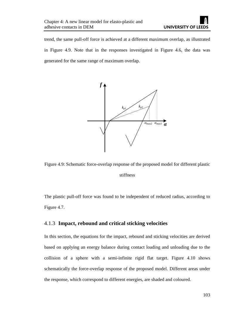
Chapter 4: A new linear model for elasto-plastic and
adhesive contacts in DEM
103
trend, the same pull-off force is achieved at a different maximum overlap, as illustrated
in Figure 4.9. Note that in the responses investigated in Figure 4.6, the data was
generated for the same range of maximum overlap.
α αmax1
f
kp1kp2
αmax2
Figure 4.9: Schematic force-overlap response of the proposed model for different plastic
stiffness
The plastic pull-off force was found to be independent of reduced radius, according to
Figure 4.7.
Impact, rebound and critical sticking velocities 4.1.3
In this section, the equations for the impact, rebound and sticking velocities are derived
based on applying an energy balance during contact loading and unloading due to the
collision of a sphere with a semi-infinite rigid flat target. Figure 4.10 shows
schematically the force-overlap response of the proposed model. Different areas under
the response, which correspond to different energies, are shaded and coloured.

Chapter 4: A new linear model for elasto-plastic and
adhesive contacts in DEM
104
Wlt
α
f
Wp
We
Wut
Figure 4.10: Schematic force-overlap response of the proposed model
In Figure 4.10 Wlt, Wp, We and Wut correspond to the initial loading tensile work, plastic
work, elastic work and unloading tensile work, respectively. The impact energy balance
from the initial velocity to the point where the sphere is brought to rest, Ei, is,
21
2i i p e ltE mv W W W (4.12)
where vi is the impact velocity. Based on this energy balance, an equation is derived for
vi,
1/22 2
max 0 0p e
i
k α α k αv
m
(4.13)
The full detailed derivation of Equation (4.13) is provided in Appendix II. It must be
noted that vi is an independent variable and in fact maximum overlap, αmax, is a function
of vi. However by rearranging the parameters, vi is given as a function of other
parameters in Equation (4.13). This enables derivations of equations for critical sticking

Chapter 4: A new linear model for elasto-plastic and
adhesive contacts in DEM
105
velocity, rebound velocity and coefficient of restitution which will be discussed in the
following sections.
It is proposed that the critical sticking velocity, vs, i.e. the maximum impact velocity for
which the contact does not break is given by,
e ut i sW W v v (4.14)
For impact velocities larger than vs, the unloading leads to detachment of the contact, as
there is sufficient elastic strain energy to overcome the work of adhesion. The rebound
velocity, vr, can be derived based on the following energy balance,
21
2r r e utE mv W W (4.15)
where Er is the rebound kinetic energy. The rebound velocity can be derived based on
Equation (4.15) (see Appendix II),
1/2
max 0 max 03 14 9 89
cp
p p cp fp c p
r
fk α α α α α α α α
vm
(4.16)
Figures 4.11-4.14 show the critical sticking velocity, vs, as a function of interface
energy, elastic stiffness, plastic stiffness and reduced radius, respectively. For all the
cases the fixed properties are as follow: ke = 1500 N/m, kp = 210 N/m, Г = 0.02 J/m2,
and R* = 2.45 μm. These conditions have been chosen to facilitate comparison with the
model of Thornton and Ning and experimental data reported in the literature (see
Section 4.1.5).

Chapter 4: A new linear model for elasto-plastic and
adhesive contacts in DEM
106
Figure 4.11: Critical sticking velocity as a function of interface energy
Figure 4.12: Critical sticking velocity as a function of elastic stiffness
0
5
10
15
20
25
30
35
40
0 0.1 0.2 0.3 0.4 0.5 0.6
Cri
tica
l st
ick
ing
vel
oci
ty (
m/s
)
Interface energy (J/m2)
0
0.2
0.4
0.6
0.8
1
1.2
1.4
1.6
1.8
0 200 400 600 800 1000 1200 1400 1600
Cri
tica
l st
ick
ing
vel
oci
ty (
m/s
)
Elastic stiffness (N/m)

Chapter 4: A new linear model for elasto-plastic and
adhesive contacts in DEM
107
Figure 4.13: Critical sticking velocity as a function of plastic stiffness
Figure 4.14: Critical sticking velocity as a function of reduced radius
The critical sticking velocity is a linear function of the interface energy and elastic
stiffness, but its relationship to plastic stiffness and reduced radius is non-linear. One
0
1
2
3
4
5
6
0 200 400 600 800 1000 1200 1400
Cri
tica
l st
ick
ing
vel
oci
ty (
m/s
)
Plastic stiffness (N/m)
0
0.2
0.4
0.6
0.8
1
1.2
1.4
1.6
1.8
2
0 20 40 60 80 100 120
Cri
tica
l st
ick
ing
vel
oci
ty (
m/s
)
Reduced radius (μm)

Chapter 4: A new linear model for elasto-plastic and
adhesive contacts in DEM
108
way of finding an equation for the sticking velocity based on single particle properties,
i.e. elastic and plastic stiffness, interface energy and reduced radius, is to determine the
best fit equations to responses in Figures 4.11-14.
The critical sticking velocity increases with increasing the interface energy since the
work of adhesion is increased and larger elastic strain energy is required to break the
contact. By increasing the elastic stiffness, the unloading elastic work is decreased and
therefore there is a reduction in the elastic strain energy. In order to compensate for this,
a larger impact velocity is required to provide a sufficiently large elastic strain energy to
break the contact. This explains the behaviour seen in Figure 4.12. The critical sticking
velocity decreases with an increase in the plastic stiffness or reduced radius. Figure 4.13
shows that the critical sticking velocity decreases with increasing the plastic stiffness.
This is due to the fact that by increasing the plastic stiffness while keeping the elastic
stiffness unchanged, the elastic strain energy is increased for a given contact force.
Figures 4.15-4.18 show the coefficient of restitution as a function of impact velocity for
different values of interface energy, elastic stiffness, plastic stiffness and reduced radius,
respectively. In all cases the fixed properties are as follow: ke = 1500 N/m, kp = 210
N/m, Г = 0.02 J/m2, and R
* = 2.45 μm.

Chapter 4: A new linear model for elasto-plastic and
adhesive contacts in DEM
109
Figure 4.15: Coefficient of restitution as a function of impact velocity for different
values of interface energy
Figure 4.16: Coefficient of restitution as a function of impact velocity for different
values of elastic stiffness
0
0.05
0.1
0.15
0.2
0.25
0.3
0.35
0.4
0 20 40 60 80 100 120 140
Co
effi
cien
t o
f re
stit
uti
on
(-)
Impact velocity (m/s)
Г = 0.02 J/m2
Г = 0.1 J/m2
Г = 0.2 J/m2
Г = 0.5 J/m2
0
0.1
0.2
0.3
0.4
0.5
0.6
0.7
0.8
0.9
0 2 4 6 8 10
Co
effi
cien
t o
f re
stit
uti
on
(-)
Impact velocity (m/s)
ke = 300 N/mke = 500 N/mke = 1100 N/mke = 1500 N/m
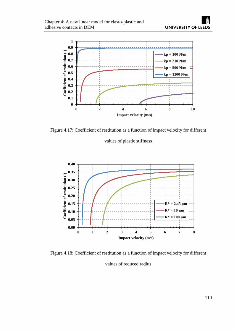
Chapter 4: A new linear model for elasto-plastic and
adhesive contacts in DEM
110
Figure 4.17: Coefficient of restitution as a function of impact velocity for different
values of plastic stiffness
Figure 4.18: Coefficient of restitution as a function of impact velocity for different
values of reduced radius
0
0.1
0.2
0.3
0.4
0.5
0.6
0.7
0.8
0.9
1
0 2 4 6 8 10
Co
effi
cien
t o
f re
stit
uti
on
(-)
Impact velocity (m/s)
kp = 100 N/m
kp = 210 N/m
kp = 500 N/m
kp = 1200 N/m
0.00
0.05
0.10
0.15
0.20
0.25
0.30
0.35
0.40
0 1 2 3 4 5 6 7 8
Co
effi
cien
t o
f re
stit
uti
on
(-)
Impact velocity (m/s)
R* = 2.45 μm
R* = 10 μm
R* = 100 μm

Chapter 4: A new linear model for elasto-plastic and
adhesive contacts in DEM
111
Generally the coefficient of restitution increases with the impact velocity because of
adhesive nature of the contact; an observation which was seen in experimental analysis
[42]. The coefficient of restitution reaches an asymptote at very high impact velocities.
The asymptotic value is a function of contact properties. Increasing the interface energy
results in a reduction of the coefficient of restitution since the cohesion is increased.
Increasing the elastic stiffness also reduces the coefficient of restitution, since the
plastic work and plastic deformation is increased. Increasing the plastic stiffness
increases the coefficient of restitution, since the contact becomes stiffer and the extent
of plastic deformation is reduced. Increasing the reduced radius increases the coefficient
of restitution, since the mass of the particles increases, subsequently the impact kinetic
energy is increased.
Linearisation of locus of pull-off force 4.1.4
Figures 4.3-4.7 showed that the locus of pull-off force is governed by the specific
surface energy and the flattened contact area. The locus is governed by an equation
which is not linear for very small deformations, yet becomes approximately linear
towards large deformations (αcp > 0.06R*
as can be seen in Figures 4.4-4.7). In an
attempt to propose a more computationally cost-effective model, the locus of the pull-
off force is considered to be a linear fit to the linear part of the locus. Hence,
0cp cp cp pf k α f (4.17)
where kcp is the slope of the linear fit and f0p is the intersection of the fit with the force-
axis. Figure 4.19 shows the pull-off force locus for αcp 0.147 μm (i.e. αcp > 0.06R*)

Chapter 4: A new linear model for elasto-plastic and
adhesive contacts in DEM
112
and the linear fit for different interface energies: ke = 1500 N/m, kp = 210 N/m, and R* =
2.45 μm.
Figure 4.19: Plastic pull-off force as a function of αcp for different interface energy
Furthermore, in a number of cases the initial elastic deformation may be small as
compared to the total deformation in which case the model can be simplified further, as
it is the case for materials with notable plastic deformation (see Section 3.4.2.3). In real
contacts, the presence of asperities always leads to plastic deformation right from the
beginning of loading. If the initial elastic deformation is ignored, the force-overlap
response can be simplified to the model that is shown schematically in Figure 4.20.
-120
-100
-80
-60
-40
-20
0
0 0.1 0.2 0.3 0.4 0.5 0.6
-fcp
(μ
N)
αcp (μm)
Г = 0.02 J/m2 Г = 0.1 J/m2 Г = 0.2 J/m2 Г = 0.5 J/m2

Chapter 4: A new linear model for elasto-plastic and
adhesive contacts in DEM
113
α
f
αp αcp αmax
α0
-fcp
-fce
αfp
-f0p
A
B
C
D
Figure 4.20: Schematic force-overlap response of the simplified model. The governing
equations are: Fn = kp(α-α0) from A to B, Fn = ke(α-αp) from B to C, and Fn = ke(2αcp-αp-
α) from C to D
Comparison of the proposed model with Luding’s, and Thornton 4.1.5
and Ning’s [15] models
Ning [44] simulated impact of an ammonium fluorescein particle to a silicon target
using Thornton and Ning’s [31] model. The parameters in their simulations are
summarised in Table 4.1.

Chapter 4: A new linear model for elasto-plastic and
adhesive contacts in DEM
114
Table 4.1: Properties of ammonium fluorescein particle and silicon wall used in Ning’s
[44] simulations
Property Particle Wall
Radius (μm) 2.45 -
Density (kg/m3) 1350 1350
Elastic modulus (GPa) 1.2 182
Poisson’s ratio (-) 0.3 0.3
Interface energy (J/m2) 0.2
Contact yield pressure (MPa) 35.3
The force-overlap response at three different impact velocities was obtained by Ning
[44] which is shown in Figure 4.21.
Figure 4.21: Normal force-overlap response of impact of an ammonium fluorescein
particle to a silicon target using Thornton and Ning’s model with three different impact
velocities [44].
-10
0
10
20
30
40
50
0 50 100 150 200 250
No
rma
l co
nta
ct f
orc
e (μ
N)
Overlap (nm)
v = 2 m/s
v = 5 m/s
v = 10 m/s

Chapter 4: A new linear model for elasto-plastic and
adhesive contacts in DEM
115
PlotDigitizer [79] software is used to digitise the response in their published work and
reproduced as Figure 4.21. In order to simulate the same system with Luding’s and the
proposed linear models, the elastic, plastic and adhesive stiffnesses are evaluated by
determining the slopes of the responses in Figure 4.21. The values are summarised in
Table 4.2.
Table 4.2: Model parameters obtained by determining the slopes of the responses in
Figure 4.21
Property Value
ke (N/m) 1500
kp (N/m) 210
kcp, kc (N/m) 20
f01, 8/9 fce (μN) 2.1
f0p (μN) 4.0
It is noteworthy that the elastic stiffness, ke, in Table 4.3 is the average value of the
initial unloading slopes in Figure 4.21. Luding’s and the proposed models were
implemented as subroutines for EDEM® software provided by DEM-Solutions,
Edinburgh, UK. The model with linear pull-off force locus is considered in these
analyses. The contact breakage is considered to be at zero force for this model, i.e. at αfp
the contact force is zero; this provides easier implementation of the model as a computer
code. It will be shown later on that this simplification does not have any significant
effect on the contact behaviour. Using the parameters in Table 4.2, a 2.45-μm radius
particle was simulated impacting a flat wall at three impact velocities; 2, 5 and 10 m/s.
The response using the proposed simplified model is shown in Figure 4.22.

Chapter 4: A new linear model for elasto-plastic and
adhesive contacts in DEM
116
Figure 4.22: Normal force-overlap responses of impact of a 2.45-μm radius particle to a
wall with the parameters in Table 4.2 using the proposed simplified model for three
different impact velocities.
Comparing Figures 4.21 and 4.22 shows a good agreement between the proposed model
and the one of Thornton and Ning in terms of maximum overlap and permanent plastic
deformation at different impact velocities. In contrast to this agreement, using Luding’s
model, the particle did not detach from the wall with impact velocities of 2, 5 and 10
m/s. Figure 4.23 shows the contact force-overlap response of the system using Luding’s
model with three different impact velocities that led to detachment. The maximum
elastic stiffness, ˆek , and the dimensionless plasticity depth, ϕf, were set to 1500 N/m
and 0.02, respectively in these simulations. The critical sticking velocity in Luding’s
model provided a maximum overlap which was larger than α*, hence the unloading
elastic stiffness was constant for the impact velocities of 15 - 25 m/s. The plastic flow
limit overlap, α*, was indeed very small (with the dimensionless plasticity depth of 0.02,
-10
0
10
20
30
40
50
0 50 100 150 200 250
No
rma
l co
nta
ct f
orc
e (μ
N)
Overlap (nm)
v = 2 m/s
v = 5 m/s
v = 10 m/s

Chapter 4: A new linear model for elasto-plastic and
adhesive contacts in DEM
117
α* is equal to ~ 0.114 μm). For the dimensionless plasticity depths larger than 0.0412,
there was always a finite rebound velocity despite extensive plastic deformation.
Figure 4.23: Normal force-overlap responses of impact of a 2.45-μm radius particle to a
wall with the parameters in Table 4.2 using Luding’s model for three different impact
velocities.
The critical sticking velocity was found to be approximately 13.8 m/s. This is due to the
fact that with Luding’s model, the adhesive work (the negative area under the curve) is
much larger compared to that of the proposed and Thornton and Ning’s model. It is
noteworthy that with an impact velocity of 13.8 m/s, the maximum overlap is
approximately 12% of the particle radius. The impact velocity by which the contact
breaks can be evaluated by applying a work balance, in a manner similar to
Section 4.1.3.
-20
0
20
40
60
80
100
120
0 100 200 300 400 500 600
No
rma
l co
nta
ct f
orc
e (μ
m)
Overlap (nm)
v = 15 m/s
v = 20 m/s
v = 25 m/s

Chapter 4: A new linear model for elasto-plastic and
adhesive contacts in DEM
118
In order to provide a more in depth comparison, the coefficient of restitution as a
function of impact velocity is compared for a range of impact velocities. The results of
the coefficient of restitution for the 2.45 μm radius ammonium fluorescein particle
impacting on the silicon target obtained by simulations using Luding’s and the proposed
models are compared with findings of Ning’s [3] in Figure 4.24. The data for Thornton
and Ning’ model were obtained by digitisation of their published work [31].
Figure 4.24: Coefficient of restitution as a function of impact velocity using different
contact models for a 2.45-μm radius ammonium fluorescein particle impacting to a
silicon target.
Figure 4.24 shows a better agreement between the proposed model and the one of
Thornton and Ning compared to Luding’s model. With the proposed model, the
coefficient of restitution initially increases however it reaches an asymptotic value of
~0.38 for impact velocities larger than ~6 m/s. The minimum impact velocity which
0
0.1
0.2
0.3
0.4
0.5
0.6
0.7
0.8
0.9
1
1 10 100
e (-
)
Impact velocity (m/s)
Thornton and Ning
Luding's model
Proposed Model

Chapter 4: A new linear model for elasto-plastic and
adhesive contacts in DEM
119
provides detachment in the proposed model is very similar to the one of Thornton and
Ning (~1.6 m/s). Thornton and Ning’s results show that the coefficient of restitution
starts reducing for impact velocities larger than ~ 10 m/s, at which the maximum
overlap is ~8.5% of the particle radius. For larger impact velocities the overlap becomes
comparable to particle size, at which point DEM simulations are not realistic due to
large deformations. Figure 4.24 also shows that the minimum impact velocity that
results in particle detachment in Luding’s model is much larger compared to that of the
proposed model and Thornton and Ning’s, 13.8 m/s compared to 1.6 m/s.
In order to verify the energy balance equations in Section 4.1.3, the analytical equation
for the coefficient of restitution as a function of impact velocity is obtained for Luding’s
and the proposed simplified models and is compared to the simulation results of
Figure 4.24. The impact velocity of Luding’s and the simplified models can be obtained
by Equation ,
1/2
2
max 0 max2p
i
kv α α α
m
(4.18)
For full detailed derivation of Equation (4.18) see Appendix III. The rebound velocity
can be calculated using Equations (4.19) and (4.20) for Luding’s and the simplified
models, respectively (see Appendices II and III).
1/2
maxmax
cp
r p p fp
fFv α α α α
m m
(4.19)
1/2
maxmax
8
9
cp
r p ce p fe
fFv α α f α α
m m m
(4.20)

Chapter 4: A new linear model for elasto-plastic and
adhesive contacts in DEM
120
where αfe is the overlap at which the unloading contact force is equal to –8/9fce. The
coefficient of restitution is analytically calculated for a range of impact velocities. The
analytical results (dotted lines) are plotted alongside the simulated results in Figure 4.25.
Figure 4.25: Coefficient of restitution as a function of impact velocity using different
contact models for a 2.45-μm radius ammonium fluorescein particle impacting to a
silicon target. The dashed lines are obtained analytically using Equations (4.19) and
(4.20).
Since the simulations results of Luding’s and the proposed model lie on the analytical
curves, it can be concluded that the energy balance considerations are correct.
The reason for the asymptotic response of the coefficient of restitution at high impact
velocities with the proposed model is attributed to a constant elastic stiffness, for which
the ratio of elastic work (We) to plastic work (Wp) is always constant. At very high
0
0.1
0.2
0.3
0.4
0.5
0.6
0.7
0.8
0.9
1
1 10 100
e (-
)
Impact velocity (m/s)
Thornton and Ning
Proposed Model
Luding's model
Analytical
Analytical

Chapter 4: A new linear model for elasto-plastic and
adhesive contacts in DEM
121
impact velocities, the elastic strain energy becomes very large relative to the work of
adhesion (Wut), so elasto-plastic process dominates since the plastic-cohesive stiffness,
kcp, is normally smaller than the plastic stiffness, kp. Hence the asymptote has a value of
(kp/ke)1/2
[14]. This asymptotic behaviour is not in line with the experimental evidence
[80, 81]. In order to account for a decreasing coefficient of restitution at high impact
velocities, the elastic unloading stiffness must be made load-dependent. Now,
considering that the stiffness increases proportionally with the contact area, which in
turn is a function of the maximum overlap, αmax, the stiffness, ke, is given by,
2 * 2
max max2ek r R α α (4.21)
where r is the contact radius. Assuming the maximum elastic stiffness, ˆek , is at an
overlap of R*, then
2
*ˆ
e e
rk k
R
(4.22)
For very small deformations, Equation (4.22) gives elastic stiffness values which can be
smaller than the plastic stiffness. In order to avoid such values for ke, following the
approach of Luding [57] as per Equation (3.74), Equation (4.22) can be modified as
follows,
2
*ˆ
e p e p
rk k k k
R
(4.23)
The maximum elastic stiffness can be evaluated by finding the tangent to the Hertz
response of the contact and finding the best match to the Hertz curve for unloading. For
the values given in Table 4.1 and Table 4.2, a maximum elastic stiffness of 13000 N/m
provided the closest agreement with the Hertz analysis.

Chapter 4: A new linear model for elasto-plastic and
adhesive contacts in DEM
122
The coefficient of restitution as a function of impact velocity is shown in Figure 4.26
for the proposed model with a load-dependent elastic unloading stiffness. This response
is obtained by the same energy balance approach as described in Section 4.1.3. The
prediction from Thornton and Ning’s model is also given for comparison.
Figure 4.26: Coefficient of restitution as a function of impact velocity using the
proposed model with a load-dependent unloading stiffness and Thornton and Ning
model.
As expected a decreasing coefficient of restitution is observed at high impact velocities,
although showing a deviation form Thornton and Ning’s model. It must be noted that
the increasing elastic stiffness is not capped here, unlike Luding’s approach, where the
elastic stiffness for overlaps larger than α* is capped. Limiting the elastic stiffness is not
physically sound since, based on the Hertz non-linear theory, the elastic stiffness
increases sharply with deformation at high loads for an elastic sphere.
0
0.1
0.2
0.3
0.4
0.5
0.6
0.7
0.8
0.9
1
1 10 100
e (-
)
Impact velocity (m/s)
Thornton and Ning
Proposed Model

Chapter 4: A new linear model for elasto-plastic and
adhesive contacts in DEM
123
Using Luding’s model with increasing elastic stiffness without capping resulted in zero
rebound velocity and hence zero coefficient of restitution for impact velocities ranging
from zero to a value that provided a deformation equal to R*. The data in Figures 4.23-
4.25 for Luding’s model were obtained for the case where the elastic stiffness was
capped at ˆek for overlaps larger than α
*. New experimental data are needed to check the
validity of models predictions, as a larger data set than that available for ammonium
fluorescein particles would provide more certaintity.
Normal contact damping 4.2
The normal damping force is a function of normal relative velocity, vr, of the two
particles in contact. The general equation for mass-spring systems is adopted here for
normal damping force [57],
nd rF βυ (4.24)
where β is the viscous damping given by Equation (4.25) ,
2 *
2 2
4ln
ln
ne m kβ
e π
(4.25)
where e is the coefficient of restitution, m* is the equivalent mass of the two particles in
contact and kn is the ‘instantaneous’ normal contact stiffness. During the initial elastic
loading and throughout the elastic unloading kn = ke and during the plastic loading kn =
kp.
Chapter 4: A new linear model for elasto-plastic and
adhesive contacts in DEM
124
Tangential model 4.3
For tangential force calculation, a linear tangential stiffness, kt, similar to the linear-
spring model is considered. Therefore the tangential force is evaluated as follow,
t t tF k α (4.26)
where αt is the tangential displacement. The sliding limit of the tangential force is
adopted from the models of Tomas [55], Luding [57] and Thornton and Yin [46]. In all
the aforementioned models a positive contribution of the normal contact force in
addition to contribution of the adhesive force is considered for defining the sliding limit.
Tomas [55] and Luding [57] stated that the reference for the contact is no longer the
zero force level, but the adhesive force level along the locus of the pull-off force. The
adhesive contribution in the proposed model is assumed to be fcp – fce, therefore the
critical tangential force (sliding limit) is given by,
ct n cp ceF μ F f f (4.27)
For the simplified version of the model, the sliding limit can also be evaluated as follow,
0ct n cp n p ceF μ F k α f f (4.28)
Sensitivity analysis of the proposed model parameters 4.4
A set of simulations are carried out in order to investigate the effects of the model
parameters on the elastic and plastic components of work during loading and unloading
of bulk compression. The simplified version of the proposed model is used. The
tangential stiffness, kt, is equated to the elastic stiffness, ke, throughout the simulations.
The model parameters for the particles are summarized in Table 4.3.

Chapter 4: A new linear model for elasto-plastic and
adhesive contacts in DEM
125
Table 4.3: Model parameter values used in the simulations
Parameter
varied kp (kN/m) ke (kN/m) Г
ke 10 50, 100,
500, 1000 0
kp
10, 50,
100, 250,
500
1000 0
kp
50, 100,
500, 1000,
2500
5000 0
ke = ke 100 100 0
Г 100 1000 0.05, 0.1,
1, 2, 5
For non-adhesive cases (i.e. when Г = 0), the model becomes identical to that of Walton
and Braun [41]. For adhesive cases, the plastic-adhesive stiffness, kcp, is kept constant at
a value of 5 kN/m. The sensitivity of bulk compression response to the plastic stiffness
(kp) is evaluated with two different fixed values of elastic stiffness (ke) in order to
achieve the same stiffness ratio (ke/kp) with different ranges of elastic and plastic
stiffnesses. This will facilitate the sensitivity analysis of stiffness ratio as well as
sensitivity of elastic and plastic stiffnesses. The walls are considered to be elastic with
zero adhesion (i.e. Г = 0, kcp = 0 and kp = ke = kt). The stiffness of the walls is set to be
8000 kN/m. 3400 particles with a mean diameter of 1 mm and a normal size distribution
(as shown in Table 4.4) are generated inside a cylindrical die of 12 mm diameter. This
number of particles provides a bed height of approximately 36 mm. The density of the
particles is set to be 1000 kg/m3.

Chapter 4: A new linear model for elasto-plastic and
adhesive contacts in DEM
126
Table 4.4: Size distribution of the generated particles
Particle
diameter (mm)
Number
frequency
(%)
0.8 5
0.9 25
1 40
1.1 25
1.2 5
The time-step is calculated based on a mass-spring system and is given by,
*
*0.2 0.2crit
crit
mt t
k (4.29)
where tcrit is the critical time-step for a mass-spring system, m* is the equivalent mass of
the smallest particle given by Equation(4.30), and k*
crit is the largest equivalent stiffness
in the system given by,
* smallest
2
mm (4.30)
where msmallest is the mass of the smallest particle in the system.
largest*
2crit
kk (4.31)
where klargest is the largest stiffness in the system. The coefficients of sliding friction and
restitution are 0.25 and 0.3, respectively for both the particle-particle and particle-wall
contacts. The compression was simulated at a strain rate of 0.28 s-1
. In order to define
the dynamics of the process, the dimensionless shear strain rate of Tardos et. al. [82] is
evaluated using following equation,

Chapter 4: A new linear model for elasto-plastic and
adhesive contacts in DEM
127
1/2
pd
g
(4.32)
where γ is the shear strain rate, dp is the mean particle diameter and g is the gravitational
acceleration. The strain rate of 0.28 s-1
provides a dimensionless shear strain rate of ~
0.003. It is shown by Tardos et. al. [82] that for dimensionless shear strain rates of <
0.15, the process is quasi-static, therefore the inertial effects on the stresses throughout
the bulk are negligible. The assembly is compressed by moving the top platen until a
bulk strain of 11% (for non-cohesive cases) or a solids fraction of 0.58 (for cohesive
cases) is achieved, after which the platen is unloaded with the same speed as during the
compression. Figure 4.27 shows a typical force-displacement curve of the top platen
during the bulk compression using DEM.
Figure 4.27: Typical loading-unloading curve of compaction (kp = 10 kN/m and ke = 50
kN/m)
0
20
40
60
80
100
120
140
160
180
200
0 0.5 1 1.5 2 2.5 3
Fo
rce
(N)
Displacement (mm)
Plastic workElastic work
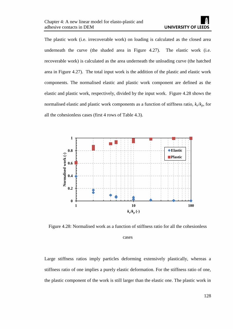
Chapter 4: A new linear model for elasto-plastic and
adhesive contacts in DEM
128
The plastic work (i.e. irrecoverable work) on loading is calculated as the closed area
underneath the curve (the shaded area in Figure 4.27). The elastic work (i.e.
recoverable work) is calculated as the area underneath the unloading curve (the hatched
area in Figure 4.27). The total input work is the addition of the plastic and elastic work
components. The normalised elastic and plastic work component are defined as the
elastic and plastic work, respectively, divided by the input work. Figure 4.28 shows the
normalised elastic and plastic work components as a function of stiffness ratio, ke/kp, for
all the cohesionless cases (first 4 rows of Table 4.3).
Figure 4.28: Normalised work as a function of stiffness ratio for all the cohesionless
cases
Large stiffness ratios imply particles deforming extensively plastically, whereas a
stiffness ratio of one implies a purely elastic deformation. For the stiffness ratio of one,
the plastic component of the work is still larger than the elastic one. The plastic work in
0
0.2
0.4
0.6
0.8
1
1 10 100
No
rma
lise
d w
ork
(-)
ke/kp (-)
Elastic
Plastic

Chapter 4: A new linear model for elasto-plastic and
adhesive contacts in DEM
129
this case has contributed towards particle rearrangements and frictional forces between
the particles and the geometry, since the contacts deform elastically. The graph shows
that as the stiffness ratio increases, the fraction of plastic work increases, while that of
elastic work decreases. The increase in the ratio means either the plastic stiffness is
decreased or the elastic stiffness is increased. If the plastic stiffness is decreased while
the elastic stiffness is kept constant (softer particles), more work is expanded in
deforming contacts to reach the same force. This leads to an increase of the total work,
while the elastic work remains the same. Therefore normalised elastic work decreases
and normalised plastic work increases. In the case where the elastic stiffness is
increased while plastic work is kept constant, the total input work does not change, but
the fraction of elastic work decreases. This leads to a decrease in the normalised elastic
work and consequently normalised plastic work increases. It can also be seen from
Figure 4.28 that there exists a limit for the stiffness ratio (ke/kp ≈ 20) beyond which
almost all of the work input into the system is used in plastic deformation.
Figure 4.29 shows the plastic and elastic works as a function of increasing the interface
energy.

Chapter 4: A new linear model for elasto-plastic and
adhesive contacts in DEM
130
Figure 4.29: Elastic and plastic work components as a function of Γ (kp = 100 kN/m, ke
= 1000 kN/m)
As it can be seen in Figure 4.29, by increasing the interface energy, the plastic work
increases; however the elastic work is very small for the range of Г investigated here
and it does not change significantly with the interface energy. An increase in the
interface energy increases the work of adhesion.
Conclusions 4.5
A new linear elasto-plastic and adhesive contact model for spherical particles has been
proposed based on improvements of Luding’s model and considering aspects of
Thornton and Ning’s and Tomas’s contact models. Plastic deformation of contacts
during loading and pure elastic unloading, accompanied by adhesion are considered, for
which the pull-off force increases with plastic deformation. Considering the collision of
a spherical cohesive body with a rigid flat target, the impact velocity that provides
contact breakage in the proposed model is found to be very similar to that of Thornton
0
2
4
6
8
10
12
14
0 1 2 3 4 5 6
Wo
rk (
mJ
)
Г (J/m2)
Plastic
Elastic

Chapter 4: A new linear model for elasto-plastic and
adhesive contacts in DEM
131
and Ning’s model. However with Luding’s model the contact breaks with a much
higher impact velocity. The coefficient of restitution as a function of impact velocity
was obtained for the proposed model and Luding’s model. The response of the proposed
model is in good agreement with the work of Thornton and Ning, however Luding’s
model underestimated the coefficient of restitution significantly.
Sensitivity analyses of the model parameters on work of compaction reveal that by
increasing the stiffness ratio (ke/kp) the normalised plastic work increases and the
normalised elastic work decreases. By increasing the interface energy, the plastic work
increases, however the elastic work does not change significantly. This highlights the
flexibility of the model in representing a wide range of particulate materials. The linear
nature of the model leads to time efficient simulations whilst still capturing the complex
material behaviour.

Chapter 5: Numerical analysis of minimum sample size and
indenter size range in ball indentation method by DEM
132
CHAPTER 5 Numerical Analysis of Minimum
Sample Size and Indenter Size
Range in Ball Indentation
Method by DEM
As discussed in Section 2.3.5, it has been shown by Hassanpour and Ghadiri [4] that
under certain circumstances, indentation on a cohesive powder bed by a blunt indenter
can give a measure of the resistance to powder flow which is related to flowability.
However, the specification of the operation window in terms of indenter size and
penetration depth has yet to be fully analysed. In this chapter, the ball indentation
process is analysed by numerical simulations using the DEM. The flow resistance of the
assembly, commonly termed hardness, is evaluated for a range of sample quantities and
operation variables.
DEM Simulation of the indentation process 5.1
Contact models 5.1.1
The calculation of the contact forces of the particles is based on the Hertz analysis for
the elastic regime. The adhesion force calculation between the particles is based on a
modified version of the theory of Johnson et al. [45], referred to as JKR model (see
Section 3.4.3.1). Figure 5.1 compares the Hertz elastic model with the JKR and the
modified version of the JKR models.

Chapter 5: Numerical analysis of minimum sample size and
indenter size range in ball indentation method by DEM
133
Figure 5.1: Comparison of force-overlap behaviour of Hertz, JKR and modified JKR
contact models
In the modified model, at the point of contact, the normal contact force immediately
drops to 8/9 of the pull-off force, similar to the JKR model. The particle velocity
reduces to zero at a point where the contact force reaches a maximum value and the
loading stage is complete. In the unloading stage, the stored elastic energy is released
and is converted into kinetic energy which makes the particle move in the opposite
direction. All the work done during the loading stage is recovered when the contact
overlap becomes zero. Based on the JKR theory, at this point, the spheres remain
adhered together and further work is required to separate the surfaces. The modified
model does not consider this additional work and the contact for this model breaks once
the overlap becomes zero. However the pull-off force required to break the contact is
representative of the JKR theory.
-1
-0.5
0
0.5
1
1.5
2
2.5
3
3.5
4
-0.4 -0.2 0 0.2 0.4 0.6 0.8 1 1.2
Co
nta
ct F
orc
e
Overlap
Hertz
JKR
Modified JKR

Chapter 5: Numerical analysis of minimum sample size and
indenter size range in ball indentation method by DEM
134
For tangential contact force calculations the no-slip solution of Mindlin [34] is used (see
Section 3.4.1.4).
Stress calculation 5.1.2
In the results section of this chapter, localised stresses amongst the powder bed are
evaluated for various operational variables. The approach that Bagi [83] introduced for
evaluation of stress in granular assemblies, is adopted here. For a localised
measurement volume, the forces acting on each particle whose centre is inside the
volume are calculated and the components of the stress tensor within the cell are
evaluated as follows,
1
p c
c p
ij i i i j
N N
x x n FV
(5.1)
where σij is the ij-component of stress tensor, V is the volume of the measurement space,
Np is number of particles in the bin, Nc is the number of contacts around particle p, c
ix ,
p
ix and ni are the i-components of contact location, particle centre and normal vector
directed from a particle centroid to its contact, respectively, and Fj is the j-component of
the contact force [83].
The localised hydrostatic and deviatoric stresses are also evaluated in the results section.
The governing equations for calculation of the hydrostatic, σhyd, and deviatoric, τD,
stresses are Equations (5.2) and (5.3), respectively.
3
xx yy zz
hyd
σ σ σσ
(5.2)

Chapter 5: Numerical analysis of minimum sample size and
indenter size range in ball indentation method by DEM
135
1/22 22
6
xx yy xx zz yy zz
D
(5.3)
This stress calculation is implemented as a subroutine for EDEM®
software. For the
details of this implementation see Appendix IV.
Simulation properties 5.1.3
16000 particles with a mean diameter of 1 mm and a Gaussian size distribution (as
shown in Table 5.1) are generated inside a cylindrical die which has a diameter (db) of
39 mm.
Table 5.1: Size distribution of the generated particles
Particle
diameter (mm)
Number
Frequency (%)
0.59 0.33
0.72 3.84
0.81 11.24
0.9 21.00
1.00 27.75
1.10 20.85
1.19 10.95
1.28 3.74
1.41 0.29
The use of a size distribution rather than a mono disperse system, avoids the formation
of ordered packing. The material properties are chosen so that they represent glass beads

Chapter 5: Numerical analysis of minimum sample size and
indenter size range in ball indentation method by DEM
136
with a cohesive interaction (Material 1) and stainless steel (Material 2), as summarised
in Table 5.2.
Table 5.2: Material properties used in the simulations
Material
property Material 1 Material 2
Young’s modulus 55 GPa 182 GPa
Poisson’s ratio 0.25 0.3
Density 2456 kg/m3 7800 kg/m
3
The particles and the indenter are made of Material 1, whereas the cylindrical die and
the piston, which is used to consolidate the bed, are made of Material 2. The interaction
properties used in the simulations are summarised in Table 5.3.
Table 5.3: Interaction properties used in the simulations
Interactional
property
Material 1-
Material 1
Material 1-
Material 2
Coefficient of
restitution 0.50 0.30
Coefficient of
sliding friction 0.15 0.0
Coefficient of
rolling friction 0.10 0.0
Interface energy 0.50 0.0
In order to avoid the influence of wall friction on the assembly, the coefficients of
sliding and rolling friction between the cylindrical die and the particles are considered
to be zero. 16000 particles provide a bed height (hb) of about 13 mm. The particles are
generated within the die and allowed to settle under gravity. The assembly is then

Chapter 5: Numerical analysis of minimum sample size and
indenter size range in ball indentation method by DEM
137
consolidated with a piston at a constant strain rate of 1 s-1
. In order to define the
dynamics of the process, the dimensionless shear strain rate of Tardos et al. [82] is
evaluated using Equation (5.4),
1/2
pd
g
(5.4)
where γ is the shear strain rate, dp is the mean particle diameter and g is the gravitational
acceleration. The strain rate of 1 s-1
provides a dimensionless shear strain rate of ~ 0.01.
It is shown by Tardos et al. [82] that for dimensionless shear strain rates of < 0.15, the
process is quasi-static, therefore the effects of the dynamics of the geometries on the
stresses throughout the bulk are minimised. For all the simulations, the assembly is pre-
consolidated to 10 kPa (σpre = 10 kPa), as this is within the realistic range of
experimental work, where results of other flowability techniques, e.g. uniaxial
unconfined compression, have been reported. Once the desired stress is achieved, the
piston is unloaded with the same speed as that of the loading. The indentation process is
simulated using a cohesionless spherical indenter made of Material 1, and the ball is
penetrated at the same constant velocity as of the piston during consolidation. The
indenter is a mesh CAD geometry imported into the software in order to facilitate strain
controlled motion of the indenter with a fixed speed.
Results and discussions 5.2
Figure 5.2 shows the hardness values calculated (see Section 2.3.5 for details of this
calculation) for a 13 mm spherical indenter on a bed of cohesive spheres for a range of
indentation loads.

Chapter 5: Numerical analysis of minimum sample size and
indenter size range in ball indentation method by DEM
138
Figure 5.2: Hardness as a function of indentation load (σpre = 10 kPa, hb = 13 mm, db =
39 mm, d = 13 mm)
At very low indentation loads/penetration depths, high values of hardness are obtained.
However, the hardness decreases very rapidly to an asymptotic value. Hardness must be
independent of indentation load in order to represent the plastic yield stress. At very
small penetration depths, the force on the indenter is due to its interactions with only a
few spheres, and hence the calculation of projected area of the impression is not suitably
described by Equation (2.9). As hardness is a continuum measure of resistance to plastic
deformation, it is necessary to identify a range for indentation load within which a
relatively constant value of hardness is obtained. The lower limit of this range should
therefore be based on the depth of penetration which initiates plastic flow in the powder
bed. The upper limit is affected by the presence of the die wall and the indenter size.
The limits of penetration depth are investigated later in this paper for a range of indenter
0
20
40
60
80
100
0 0.2 0.4 0.6 0.8 1
Ha
rdn
ess
(kP
a)
Indentation load (N)

Chapter 5: Numerical analysis of minimum sample size and
indenter size range in ball indentation method by DEM
139
sizes. In order to compare the results of different indenter sizes, a dimensionless
penetration, hd, as defined by Equation (5.5), is considered.
d
hh
r (5.5)
where h is the penetration depth and r is the radius of the indenter. Figure 5.3 shows the
hardness against dimensionless penetration for an indenter size of 13 mm and at 10 kPa
pre-consolidation pressure. In order to disregard the artificially high values of hardness
that occur at the start of the indentation process, the data are presented for
dimensionless penetrations greater than that corresponding to one particle diameter.
Figure 5.3: Hardness as a function of dimensionless penetration (σpre = 10 kPa, hb = 13
mm, db = 39 mm, d = 13 mm)
It can be seen that initially there are fluctuations in the hardness value, however, after a
dimensionless penetration of about 0.4, the hardness stabilises around 8 kPa. This
behaviour can be attributed to the fact that for low penetration depths the plastic flow in
0
2
4
6
8
10
12
0 0.2 0.4 0.6 0.8 1
Ha
rdn
ess
(kP
a)
Dimensionless Penetration (-)

Chapter 5: Numerical analysis of minimum sample size and
indenter size range in ball indentation method by DEM
140
the bed is not fully initiated. Figure 5.4 shows hardness against dimensionless
penetration for indenter sizes of 16 and 19 mm.
Figure 5.4: Hardness as a function of dimensionless penetration (σpre = 10 kPa, hb = 13
mm, db = 39 mm)
For these indenter sizes initial fluctuations in the hardness value are also present, but
after a dimensionless penetration of about 0.35, the hardness stabilises around 8 kPa.
Figure 5.5 shows the hardness against dimensionless penetration for indenter sizes of 7
and 10 mm.
0
2
4
6
8
10
12
14
0 0.2 0.4 0.6 0.8 1
Ha
rdn
ess
(kP
a)
Dimensionless Penetration (-)
d=16mm
d=19mm

Chapter 5: Numerical analysis of minimum sample size and
indenter size range in ball indentation method by DEM
141
Figure 5.5: Hardness as a function of dimensionless penetration (σpre = 10 kPa, hb = 13
mm, db = 39 mm)
As it can be seen, the hardness exhibits wider fluctuations than previously observed for
the larger indenters within the whole range of penetration depths investigated here.
These fluctuations are significantly larger for smaller penetration depths and smaller
indenter diameters. As the indenter size decreases, approaching the size of bed particles,
particle rearrangements at the single particle level become more prominent and
substantially influence the force on the indenter throughout the indentation process,
resulting in fluctuations, whereas the number of particle-indenter contacts increases if
the indenter size is increased. This leads to a reduction in the fluctuations of force acting
on the indenter. Moreover, small indenters may introduce localised consolidation,
resulting in measuring a greater hardness. Figure 5.6 shows the hardness against
dimensionless penetration for the indenter sizes of 22 and 25 mm.
0
2
4
6
8
10
12
14
0 0.2 0.4 0.6 0.8 1
Ha
rdn
ess
(kP
a)
Dimensionless Penetration (-)
d=7mm
d=10mm

Chapter 5: Numerical analysis of minimum sample size and
indenter size range in ball indentation method by DEM
142
Figure 5.6: Hardness as a function of dimensionless penetration (σpre = 10 kPa, hb = 13
mm, db = 39 mm)
After initial fluctuations with these larger indenter sizes, the hardness value is stabilised
around 10 kPa, which is larger than those measured by smaller indenters (13-19 mm in
diameter). With large indenters, the indent size may be affected by the surrounding wall.
In order to examine the wall effects with larger indenters, the particle assembly is
plotted at three different penetration depths using the 25 mm indenter in Figure 5.7. The
grey-scale of each particle in Figure 5.7 indicates its velocity, with lighter particles
having negligible velocity.
0
2
4
6
8
10
12
14
0 0.2 0.4 0.6 0.8 1
Ha
rdn
es (
kP
a)
Dimensionless penetration(-)
d=22mm
d=25mm

Chapter 5: Numerical analysis of minimum sample size and
indenter size range in ball indentation method by DEM
143
Figure 5.7: Indentation process using the 25 mm indenter (a) hd = 0.0 (b) hd = 0.27 (c)
hd = 0.49
It can be seen that the whole bed is deforming during the indentation process at greater
penetration depths (Figure 5.7c), as indicated by the particles neighbouring the die wall.
The surrounding walls are therefore restricting the bed deformation, which leads to an
increase in the resistance of the bed against shear deformation and hence an increase in
hardness. In order to investigate the wall effects in more detail, localised stresses and
particle velocities are evaluated for various indenter sizes. For this purpose, a cuboid
region centrally aligned with the axis in the cylindrical die is considered for the analysis
(Figure 5.8a). The cuboid region is divided into 15 bins, each of which has dimensions
of 5.2, 5.2 and 4.2 mm in x, y and z directions, respectively (Figure 5.8).

Chapter 5: Numerical analysis of minimum sample size and
indenter size range in ball indentation method by DEM
144
Figure 5.8: Cuboid bins used for localised velocity and stresses analysis: (a) side view
(b) plan view (dimensions are normalised by mean particle size, which is 1 mm)
The height of the cuboid region approximates the bed height. This region is not
extended to the walls in order to avoid an excessive number of bins. Within each bin,
the forces acting on each particle whose centre is inside this cell are calculated and the
components of the stress tensor within the cell are evaluated as discussed in
Section 5.1.2. The hydrostatic and deviatoric stresses are also evaluated. The stress
calculations for each bin are carried out as the indenter is penetrating the bed. Once the
indenter is inside a bin, the calculation volume in Equation (5.1) is reduced to the
volume of the bin which is not occupied by the indenter. The calculation of effective bin
volume due to the interaction between the spherical indenter and cuboid bins is
mathematically complex; hence the stress calculations are performed only for the range
of depths within which the indenter does not have an intersection with the bin under
consideration. The deviatoric and hydrostatic stresses within each of the bins for
indenter diameters of 7, 13 and 25 mm are shown in Figures 5.9-5.11, respectively.

Chapter 5: Numerical analysis of minimum sample size and indenter size range in ball indentation
method by DEM
145
Figure 5.9: Hydrostatic and deviatoric stresses within the cuboid bins (σpre = 10 kPa, hb = 13 mm, db = 39 mm, d = 7 mm)

Chapter 5: Numerical analysis of minimum sample size and indenter size range in ball indentation
method by DEM
146
Figure 5.10: Hydrostatic and deviatoric stresses within the cuboid bins (σpre = 10 kPa, hb = 13 mm, db = 39 mm, d = 13 mm)

Chapter 5: Numerical analysis of minimum sample size and indenter size range in ball indentation
method by DEM
147
Figure 5.11: Hydrostatic and deviatoric stresses within the cuboid bins (σpre = 10 kPa, hb = 13 mm, db = 39 mm, d = 25 mm)

Chapter 5: Numerical analysis of minimum sample size and
indenter size range in ball indentation method by DEM
148
For the 7 mm indenter, the stresses do not vary significantly within all the bins, except
for the bin directly below the indenter (bin: 32) which exhibits the highest stress level.
In this case, the bin width is greater than the projected diameter of impression for most
of the penetration depth. This may explain the negligible increase in force in all regions
except for bin 32. For both the 13 and 25 mm indenters, the stresses close to the bottom
of the die (bins: 21, 31and 41) are notable, indicating interactions with the die base. The
bins close to the die cylindrical wall (bins: 11, 12, 51, and 52) show high levels of stress
only with the 25 mm indenter. These analyses show that with larger indenters the
stresses close to the die base are relatively large and the stresses close to the die wall
may also be large. This indicates that the die in this case provides a resistance to the bed
shear deformation caused by the indenter. It is necessary to have a sufficiently large
clearance between the edge of the indentation zone and the die wall and the base, such
that the plastic flow of the powder is not restrained by the boundaries. The principle of
flowability measurement using this technique relies upon establishing a constraint factor,
i.e. the ratio between hardness and plastic yield stress for a given material. If the
indenter diameter is too large the constraint factor will increase due to the wall effects,
rather than being purely determined by the shear zone.
In order to clarify the influence of wall confinement on hardness measurements, a wider
range of simulations is required. By varying the bed height and die diameter, the
minimum sample quantity which is required to reliably measure hardness by ball
indentation can be determined. Therefore in addition to the simulations with a bed
height of 13 mm and a bed diameter of 39 mm, a series of simulations are performed for
a die diameter of 45 mm and bed heights of 20, 30 and 50 mm, using a 13 mm indenter.

Chapter 5: Numerical analysis of minimum sample size and
indenter size range in ball indentation method by DEM
149
Hardness against dimensionless penetration for these four simulations is shown in
Figure 5.12.
Figure 5.12: Hardness vs. dimensionless penetration for four different bed heights (σpre
= 10 kPa, d = 13 mm)
For all of the bed heights, initial fluctuations in hardness can be observed; however, bed
heights of 20, 30 and 50 mm exhibit lower hardness values (about 6 kPa) than the 13
mm bed height (about 8 kPa). Since for the larger bed heights a relatively constant
hardness can be obtained, the simulations for this range of bed heights are not
influenced by confinement at the base. This is shown to be the case by detailed analyses
of the internal stresses and velocities, similar to those carried out for the 13 mm bed
height. As compared to the bin analysis for the 13 mm bed height, the cuboid region
here is extended by 1 row of cuboid bins towards the die base for the bed height of 20
mm (Figure 5.13) in order to analyse the stresses throughout the assembly.

Chapter 5: Numerical analysis of minimum sample size and
indenter size range in ball indentation method by DEM
150
Figure 5.13: Cuboid bins used for localised velocity and stress analysis for 20 mm bed
height (a) side view (b) plan view (dimensions are normalised by mean particle size
which is 1 mm)
The internal stresses inside each bin are shown in Figure 5.14.

Chapter 5: Numerical analysis of minimum sample size and indenter size range in ball indentation
method by DEM
151
Figure 5.14: Hydrostatic and deviatoric stresses within cuboid bins (σpre = 10 kPa, hb = 20 mm, db = 45 mm, d = 13 mm)

Chapter 5: Numerical analysis of minimum sample size and
indenter size range in ball indentation method by DEM
152
As it can be seen, the stresses decrease to negligible levels towards the base and
cylindrical walls. Near the base, these stresses are negligible. This is another indication
that for this scale of simulation, the wall confinement is not influencing the hardness.
With the minimum sample size in terms of bed height and bed diameter now determined,
a sensitivity analysis for a range of indenter sizes is carried out to reveal the effect of
indenter size on hardness measurement. The same range of indenter sizes as of the
previous case is used here to simulate ball indentation on the 20 mm bed height. The
bed is pre-consolidated to 10 kPa. Figure 5.15 shows hardness against dimensionless
penetration for indenter sizes of 16, 19 and 22 mm.
Figure 5.15: Hardness as a function of dimensionless penetration (σpre = 10 kPa, hb =
20mm, db = 45 mm)
0
1
2
3
4
5
6
7
8
0 0.2 0.4 0.6 0.8 1
Ha
rdn
ess
(kP
a)
Dimensionless Penetration (-)
d=16mm
d=19mm
d=22mm

Chapter 5: Numerical analysis of minimum sample size and
indenter size range in ball indentation method by DEM
153
As compared to the 13 mm bed height system (Figures 5.3-5.6), the hardness shows
smaller fluctuations. For this range of indenter sizes, a relatively constant value of
hardness (about 6 kPa) is obtained. Figure 5.16 shows the hardness as a function of the
dimensionless penetration for indenter diameters of 7, 10 and 13 mm, bed height of 20
mm and bed diameter of 45 mm.
Figure 5.16: Hardness as a function of dimensionless penetration (σpre = 10 kPa, hb = 20
mm, db = 45mm)
As compared to the larger indenters (16-22 mm in Figure 5.15), the fluctuations within
the whole range of dimensionless penetration depths are larger for indenter diameters of
7, 10 and 13 mm. Similar to the 13 mm bed height case, this can be attributed to the fact
that the smaller indenters are comparable in size to single particles, and rearrangements
at the single particle level influence the force on the indenter throughout the indentation
process, resulting in instabilities. The increase in fluctuations with decreasing the
0
1
2
3
4
5
6
7
8
0 0.2 0.4 0.6 0.8 1 1.2
Ha
rdn
ess
(kP
a)
Dimensionless penetration (-)
d=7mm
d=10mm
d=13mm

Chapter 5: Numerical analysis of minimum sample size and
indenter size range in ball indentation method by DEM
154
indenter size can be quantitatively observed in Figure 5.17, by the range of fluctuations
as it widens for smaller indenters.
Figure 5.17: Average hardness with fluctuation bars indicating standard deviation for
different indenter sizes (σpre = 10 kPa, hb = 20 mm, db = 45mm)
It can be concluded that the indenter size should be greater than 13 particle diameters,
with 16 diameters being adequate.
With the minimum sample size and suitable indenter size now determined, the operation
window for the penetration depth is investigated by calculation of hydrostatic stress
inside a dynamic bin directly below and centrally aligned with the indenter, whose
position is fixed relative to the indenter, i.e. it moves with the indenter (see Figure 5.18).
The size of the bin is the same as the individual bins in the previous analyses, i.e. 5.2,
5.2 and 4.2 mm in x, y and z directions, respectively.
0
1
2
3
4
5
6
7
8
0 5 10 15 20 25
Ha
rdn
ess
(kP
a)
Indenter diameter / particle mean diameter (-)

Chapter 5: Numerical analysis of minimum sample size and
indenter size range in ball indentation method by DEM
155
5.2 mm
4.2 mm
x
z
5.2 mm
4.2 mm
(a) (b)
Figure 5.18: Schematic diagram of the dynamic bin underneath the indenter at two
different penetration depths
Figure 5.19 shows the hydrostatic stress inside this bin for indenter diameters of 7, 16,
19 and 22 mm, a bed height of 20 mm and a bed diameter of 45 mm.
Figure 5.19: Hydrostatic stress inside the dynamic bin as a function of dimensionless
penetration for different indenter sizes (σpre = 10 kPa, hb = 20 mm, db = 45mm)
0
1
2
3
4
5
6
0 0.2 0.4 0.6 0.8 1 1.2
Str
ess
(kP
a)
Dimensionless penetration (-)
d = 7 mm
d = 16 mm
d = 19 mm
d = 22 mm

Chapter 5: Numerical analysis of minimum sample size and
indenter size range in ball indentation method by DEM
156
For the suitable indenter sizes, i.e. 16, 19 and 22 mm indenters, the hydrostatic stress
increases initially up to a dimensionless penetration of about 0.1. Beyond this point the
stress has a relatively constant average value, although fluctuating. This is the region of
interest where the flow stress is calculated. For dimensionless penetrations beyond 0.5,
the stress starts increasing again, which indicates the influence of a number of factors
depending on the proximity of the walls and the base and ultimate penetration depth.
For the 7-mm indenter, it is difficult to determine a range for constant value of hardness
due to large fluctuations.
Conclusions 5.3
The ball indentation on a compacted assembly of cohesive spheres was simulated using
DEM. The hardness of the compacted assembly was evaluated for a range of sample
quantities. It was found that a minimum bed height of 20 particle diameters is required
in order to achieve reliable hardness values. With small sample sizes, for which the
surrounding walls and base of the die restrain the bed deformation, an increase in the
resistance of the bed, i.e. an increase in hardness, is observed. It is necessary to have a
sufficiently large clearance between the edge of the indentation zone and the die wall,
such that the plastic flow of the powder is not restrained. The penetration depth is
normalised with respect to the indenter radius in order to allow the effect of different
indenter sizes to be analysed and compared. The penetration depth should be
sufficiently large to cause notable bed shear deformation. It is found that this minimum
penetration depth is approximately equal to 0.1 in terms of dimensionless penetration. A
sensitivity analysis of indenter size reveals that indenters with diameters smaller than 16
particle diameters exhibit fluctuations in hardness measurements, whereas indenters

Chapter 5: Numerical analysis of minimum sample size and
indenter size range in ball indentation method by DEM
157
with a diameter of up to 22 particle diameters result in stable hardness values, providing
the minimum sample criteria are met. As the indenter size decreases, it approaches the
size of bed particles. Therefore, rearrangements at the single particle level influence the
force on the indenter throughout the indentation process, resulting in fluctuations in
hardness. With very large indenters comparable in size to the die, the measurement of
hardness may be affected by the wall.

Chapter 6: Sensitivity analysis of indenter and single particle
properties in ball indentation method by DEM
158
CHAPTER 6 Sensitivity Analysis of Indenter
and Single Particle Properties in
Ball Indentation Method by
DEM
With the minimum sample size, suitable indenter size and penetration depth determined
numerically in Chapter 5, the operation window for the indenter properties such as
shape, stiffness and friction is investigated in this chapter. Moreover variation of
hardness and internal stresses with single particle properties such as inter-particle
friction and cohesion are analysed by DEM simulations of the ball indentation process.
DEM simulation of the indentation process 6.1
For DEM simulations reported in this chapter, the simplified version of the proposed
contact model discussed in Chapter 4 is used (see Figure 4.20). The simulations are
based on meeting the criteria defined in Chapter 5. The sample height and diameter are
20 and 45 mean particle diameters, respectively. The indentation process was simulated
using a 16 mm indenter. The simulations are conducted using EDEM® software
provided by DEM Solutions, Edinburgh, UK.
Particles with a normal size distribution and a mean diameter of 1 mm (as shown in
Table 6.1) are generated inside the cylindrical die. The use of a size distribution rather

Chapter 6: Sensitivity analysis of indenter and single particle
properties in ball indentation method by DEM
159
than a mono disperse system avoids the formation of ordered packing. In order to
provide a bed height of approximately 20 mm, 29000 particles are generated.
Table 6.1: Size distribution of the generated particles
Particle
diameter (mm)
Number
Frequency (%)
0.724 3.87
0.814 11.31
0.896 21.14
1.000 27.92
1.104 20.99
1.188 11.02
1.278 3.76
1.28 3.74
1.41 0.29
The tangential stiffness, kt, was equated to the elastic stiffness, ke, throughout the
simulations. The material and interactional properties of the elasto-plastic-adhesive
particles and the non-cohesive elastic geometries (indenter, cylindrical die and piston)
are summarised in Tables 6.2 and 6.3.

Chapter 6: Sensitivity analysis of indenter and single particle
properties in ball indentation method by DEM
160
Table 6.2: Material properties used in the simulations
Material property Particles Geometries
Density (kg/m3) 2500 7800
Poisson’s ratio (-) 0.25 0.3
Elastic stiffness, ke (MN/m) 1 8
Plastic stiffness, kp (MN/m) 0.1 -
Plastic-adhesive stiffness, kcp (MN/m) 0.01 -
Tangential stiffness, kt (MN/m) 1 8
Table 6.3: Interaction properties used in the simulations
Interactional property Particle - Particle Particle - Wall
Coefficient of restitution (-) 0.50 0.30
Coefficient of sliding friction (-) 0.15 0.0
Coefficient of rolling friction (-) 0.01 0.0
Interface energy (J/m2) 2.00 0.0
The particles are generated within the die, ascribed the properties as given in Tables 6.1-
6.3 and allowed to settle under gravity. The assembly is then consolidated with a piston
at a constant strain rate of 1 s-1
to 10 kPa. Once the desired stress is achieved, the piston
is unloaded with the same speed as that of the loading, similar to the simulations of
Chapter 5.
As in the analysis of Chapter 5, a dynamic bin with dimensions of 5.2, 5.2 and 4.2 mm
in x, y and z-directions, respectively was considered. The hydrostatic and deviatoric

Chapter 6: Sensitivity analysis of indenter and single particle
properties in ball indentation method by DEM
161
stresses inside this dynamic bin are evaluated and the results are compared to the
hardness value measured by the indenter (see Section 5.1.2).
Sensitivity analysis of indenter properties 6.2
Indenter stiffness 6.2.1
The simulations were carried out for a wide range of indenter stiffness. The result of
hardness, hydrostatic and deviatoric stresses as functions of indenter stiffness is shown
in Figure 6.1.
Figure 6.1: Hardness, hydrostatic and deviatoric stresses as functions of indenter
stiffness
As it can be seen, there is hardly any effect of indenter stiffness in hardness, or
hydrostatic and deviatoric stress measurement in the ball indentation method.
0
2
4
6
8
10
12
14
16
0.1 1 10 100 1000 10000
Str
ess
(kP
a)
Indenter Stiffness (kN/m)
Hardness Hydrostatic Deviatoric

Chapter 6: Sensitivity analysis of indenter and single particle
properties in ball indentation method by DEM
162
Indenter shape 6.2.2
The simulations were carried out with three different indenter shapes: cubic, cylindrical
and spherical indenters. The spherical and cylindrical indenters had a diameter of 16
mm, while the cubic indenter had equal sides of 16 mm. Figure 6.2 shows hardness,
hydrostatic and deviatoric stresses measured by the three different indenter shapes.
Figure 6.2: Hardness, hydrostatic and deviatoric stresses measured by the three different
indenter shapes
The hardness measured by cubic and cylindrical indenters is higher to that measured by
a spherical indenter. The internal stresses within the dynamic bin do not change
significantly with indenter shape. In order to illustrate this behaviour qualitatively,
Figure 6.3 shows the assembly at the same penetration depth using the three indenter
shapes. The colour-scale of each particle in Figure 6.3 indicates its velocity, with blue
particles having negligible velocity and red particles with large velocity. The colour
0
5
10
15
20
25
Cubic Cylindrical Spherical
Str
ess
(kP
a)
Hardness
Hydrostatic
Deviatoric

Chapter 6: Sensitivity analysis of indenter and single particle
properties in ball indentation method by DEM
163
range for all the three cases is the same; minimum (blue) is 0.002 m/s and maximum
(red) is 0.04 m/s.
Figure 6.3: DEM simulation of indentation technique using (a) cubic, (b) cylindrical and
(c) spherical indenters at penetration depth of 3.8 mm. For visualisation purposes, the
assembly is clipped by a plane y-direction. The particles are coloured based on their
magnitude of velocity (red, green and blue indicate high to low velocities)
As it can be seen, the particles close to the bottom base and surrounding wall show
some velocity (i.e. particle movement) for cubic and cylindrical indenters, in contrast to
the spherical case. This suggests that cylindrical and cubical indenters must be smaller
for this bed height, or the bed height must be larger.
Close inspection of data on which Figure 6.3 is based indicated that there is an increase
in solids fraction with cubic and cylindrical indenters relative to the spherical case. In
order to investigate this behaviour quantitatively, the solids fraction in a bin with
dimensions of 0.01, 0.01 and 0.012 in x, y and z-directions, respectively, which is
located in the centre of the cylindrical die (see Figure 6.4) is evaluated as a function of
penetration depth for the three indenter shapes.

Chapter 6: Sensitivity analysis of indenter and single particle
properties in ball indentation method by DEM
164
10 mm 10 mm
10 mm
12 mm
x
z
x
y
(a) (b)
Figure 6.4: The cuboid bin used for solids fraction analysis: (a) side view (b) plan view
Figure 6.5 shows the solids fraction inside the cuboid bin as a function of penetration
depth for the three indenter shapes.
Figure 6.5: Solids fraction inside the cuboid bin as a function of penetration depth for
three different indenter shapes
0.56
0.565
0.57
0.575
0.58
0.585
0 1 2 3 4 5 6 7 8
So
lid
s fr
act
ion
(-)
Penetration depth (mm)
Spherical
Cubic
Cylidrical

Chapter 6: Sensitivity analysis of indenter and single particle
properties in ball indentation method by DEM
165
As it can be seen, the solids fraction is increased for cubic and cylindrical indenters
relative to the spherical indenter, an indication of localised consolidation with
cylindrical and cubic indenters. In fact, the curvature of a sphere results in a smoother
transition from elastic to plastic behaviour and allows the powder to be sheared rather
than being consolidated.
Indenter friction 6.2.3
The simulations were also conducted for a range of indenter coefficient of sliding
friction between the particles and the spherical indenter (i.e. indenter friction). The
results of hardness, hydrostatic and deviatoric stresses are shown in Figure 6.6.
Figure 6.6: Hardness, hydrostatic and deviatoric stresses as functions of indenter friction
A general increasing trend in the stresses with indenter friction can be observed. This
increase is notable when the coefficient of sliding friction is increased from zero to 0.1.
Increasing the sliding friction of the indenter provides additional resistance to shearing
0
2
4
6
8
10
12
14
16
18
20
0 0.1 0.2 0.3 0.4 0.5 0.6
Str
ess
(kP
a)
Indenter friction (-)
Hardness Hydrostatic Deviatoric

Chapter 6: Sensitivity analysis of indenter and single particle
properties in ball indentation method by DEM
166
of the particles contacting the indenter, consequently the hardness, which is evaluated
by the force acting on the indenter is increased.
Effects of single particle properties 6.3
Inter-particle friction 6.3.1
Figure 6.7 shows hardness, hydrostatic and deviatoric stresses as functions of inter-
particle coefficient of sliding friction.
Figure 6.7: Hardness, hydrostatic and deviatoric stresses as functions of inter-particle
coefficient of sliding friction
Increasing the inter-particle friction would increase the internal resistance to shear
deformation, an observation which was expected. It can be observed that there is a limit
for the sliding friction coefficient beyond which the stresses do not change (compare μs
= 0.3 and 0.5 in Figure 6.7). This can be attributed to the fact that, within the
0
5
10
15
20
25
0 0.1 0.2 0.3 0.4 0.5 0.6
Dev
iato
ric
stre
ss (
kP
a)
Sliding friction coefficient (-)
Hardness
Hydrostatic
Deviatoric

Chapter 6: Sensitivity analysis of indenter and single particle
properties in ball indentation method by DEM
167
indentation process, the tangential force at the single particle does not become large
enough to meet the Coulomb’s criterion of sliding. In other words, for highly frictional
contacts, contact sliding does not occur. The sliding is indeed a dominant factor in shear
deformation of the assembly. It can be concluded from Figure 6.7 that when inter-
particle coefficient of sliding friction is larger than 0.3, the contact sliding behaviour
becomes similar.
Inter-particle cohesion 6.3.2
Figure 6.8 shows hardness, hydrostatic and deviatoric stresses as functions of inter-
particle interface energy.
Figure 6.8: Hardness, hydrostatic and deviatoric stresses as functions of inter-particle
interface energy
As it was expected, increasing the cohesion increases hardness and internal stresses,
since the resistance to flow is increased
0
10
20
30
40
50
60
0 5 10 15 20 25
Str
ess
(kP
a)
Interface energy (J/m2)
Hardness
Hydrostatic
Deviatoric

Chapter 6: Sensitivity analysis of indenter and single particle
properties in ball indentation method by DEM
168
Conclusions 6.4
The ball indentation on a compacted assembly of cohesive spheres was simulated using
DEM. The hardness and localised hydrostatic and deviatoric stresses were evaluated for
various indenter and inter-particle properties. The hardness measurements were found to
be independent of indenter stiffness. Indenter friction slightly increased the hardness,
although its influence on the internal stresses was negligible. Cubic and cylindrical
indenters measured significantly larger hardness value compared to the spherical
indenter. It was shown that with cubic and cylindrical indenters, the powder bed is
locally consolidated, hence the measured value of hardness is not representative of the
bulk consolidation state. Increasing the inter-particle friction and cohesion resulted in
higher hardness and internal stresses due the increase in resistance to shear deformation.

Chapter 7: Numerical analysis of strain rate sensitivity in
ball indentation method by DEM
169
CHAPTER 7 Numerical Analysis of Strain
Rate Sensitivity in Ball
Indentation Method by DEM
In industrial processes such as mixing, blending, handling and storage reliable powder
flow is important for product quality and a consistent production rate. Understanding
the flow characteristics of the powder can avoid wastage, machinery maintenance
problems and downtime in such processes. Strain rate is particularly of great interest
since in the shear deformation of powder beds beyond the quasi-static regime the shear
stress is dependent on the strain rate [82]. Extensive work has been reported on the
rapid chute flow of large granules [84] but the intermediate regime has not been widely
addressed. However, the industrial powder processes require the specification of an
operational window in terms of strain rate for reliable and controllable operations.
Tardos et al. [82] classified powder flow into three regimes based on the shear strain
rate of the process. At low shear strain rates, the quasi-static regime can be identified,
during which frictional forces between particles are predominant and the shear stress is
independent of the strain rate. In the other extreme at very high shear strain rates, i.e.
the dynamic regime, the flow is characterised by collisions between particles rather than
the friction between them and hence the particle inertia is influential. There has been
extensive work for this regime, in which it has been shown that the shear stress varies
with the square of strain rate [85-87]. Between the quasi-static and inertial regimes lies
the intermediate regime, where both collisional and frictional interactions between the

Chapter 7: Numerical analysis of strain rate sensitivity in
ball indentation method by DEM
170
particles determine the flow characteristics [82]. Many of the flowability measurement
techniques (see Section 2.4) evaluate the incipient flow at very low strain rates (i.e. the
quasi-static regime), and hence cannot depict the strain rate sensitivity of powder flow.
The only method by which the intermediate regime has been analysed is the Coutte
device of Tardos et al. [82], where the powder is sheared between two concentric
cylinders (with the axis being vertical). The inner cylinder is rotated at different
rotational velocity forming a shear band in the gap. It was confirmed that during the
quasi-static regime the stresses were independent of the strain rate. For the intermediate
regime the dependency of the shear stress on the dimensionless strain rate γ* (as given
by Equation (7.1) ) is with a power index less than 2.
1/2
* pd
g
(7.1)
where γ is the shear strain rate, dp is the mean particle diameter and g is the gravitational
acceleration. For the dynamic regime, this dependency is to a power of 2 [88]. By
increasing the strain rate, an increase in the fluctuations of the stresses was observed. It
was shown that the width of the intermediate regime in terms of dimensionless shear
rate is a function of assembly concentration [82]. At low particle concentration (high
bed porosity), the width was relatively narrow, between dimensionless shear rates of 0.5
to 2 [82].
In two commercial developments, proprietary instruments also subject the powder to
shear strains in the intermediate regime by a paddle penetrating whilst rotating in a
powder bed (Freeman Powder Tester FT4 [89] and StableMicro Systems PowderFlow
Analyser). However the complex paddle geometry provides a highly non-uniform strain

Chapter 7: Numerical analysis of strain rate sensitivity in
ball indentation method by DEM
171
field, where the powder strain and strain rate increase from the centre to the cylindrical
wall. Recently Hare et al. [54] have analysed the shear stress and strain field around a
rotating impeller and have quantified their radial and axial variations. Their work shows
that the shear stress is greatest in the vicinity of the front of the blades; the stresses
reduce above the impeller and away from the impeller in the angular direction,
providing a highly non-uniform strain field. Based on their work, the interpretation of
paddle torque to elucidate the strain rate dependency of shear stresses using these
commercial devices is difficult until systematic work on model materials with ‘tuneable’
and controlled bulk cohesion has been fully analysed.
Moreno-Atanasio et al. [90] simulated uniaxial unconfined compression of cohesive
beds using the Distinct Element Method (DEM) for a range of strain rates. They also
found that the unconfined yield stress (UYS) did not depend on strain rate for small
values of strain rate (less than 2 s-1
), and only exhibited dependency for larger values,
where a linear relationship between UYS and strain rate was reported. A power law fit
with a power index of 1.2 showed the best fit for the simulations data. The threshold
strain rate which defined the limiting quasi-static rate was found to be slightly
dependent on the inter-particle cohesion, where by increasing the cohesion the threshold
was increased slightly. It was also shown that by increasing the pre-consolidation stress,
the sensitivity of UYS to the strain rate decreased in the intermediate and dynamic
regimes, which was in-line with Tardos et al. [82] findings on assembly concentration.
It should be noted that possible effects of aeration were not considered in the above
analysis.

Chapter 7: Numerical analysis of strain rate sensitivity in
ball indentation method by DEM
172
In the present chapter the strain rate sensitivity of the stresses in an assembly of
cohesive spherical particles within the ball indentation process is investigated using
DEM. Again, the effect of air drag in this analysis is ignored.
DEM simulations of the indentation process 7.1
The simulations properties are the same as the ones reported in Chapter 6 (see
Section 6.1). The simplified version of the proposed contact model discussed in Chapter
4 is used (see Figure 4.20). The simulations are based on meeting the criteria defined in
Chapter 5. The sample height and diameter are 20 and 45 mean particle diameters,
respectively. The indentation process was simulated using a 16 mm indenter. The
simulations are conducted using EDEM® software provided by DEM Solutions,
Edinburgh, UK. Particle and geometry properties are summarised in Tables 6.1-6.3.
The particles are generated within the die and allowed to settle under gravity. The
assembly is then consolidated with a piston at a constant strain rate of 1 s-1
to 10 kPa.
Once the desired stress is achieved, the piston is unloaded with the same speed as that of
the loading, in a similar manner to the simulations of Chapters 5 and 6.
As in the analysis of Chapters 5 and 6, a dynamic bin with dimensions of 5.2, 5.2 and
4.2 mm in x, y and z-directions, respectively was considered. The hydrostatic and
deviatoric stresses inside this dynamic bin are evaluated and the results are compared to
the hardness value measured by the indenter (see Section 5.1.2).

Chapter 7: Numerical analysis of strain rate sensitivity in
ball indentation method by DEM
173
Sensitivity of hardness, hydrostatic and deviatoric 7.2
stresses to strain rate
Figures 7.1(a)-(d) show hardness, hydrostatic and deviatoric stresses inside the dynamic
bin as functions of dimensionless penetration for dimensionless strain rates of 0.0115,
0.2297, 0.4594 and 2.2969, respectively.
0
2
4
6
8
10
12
14
16
0 0.2 0.4 0.6 0.8 1
Str
ess
(kP
a)
Dimensionless penetration (-)
(a) γ* = 0.0115
Hardness
Hydrostatic
Deviatoric

Chapter 7: Numerical analysis of strain rate sensitivity in
ball indentation method by DEM
174
0
2
4
6
8
10
12
14
16
18
20
0 0.2 0.4 0.6 0.8 1
Str
ess
(kP
a)
Dimensionless penetration (-)
(b) γ* = 0.2297
Hardness
Hydrostatic
Deviatoric
0
5
10
15
20
25
30
35
0 0.2 0.4 0.6 0.8 1
Str
ess
(kP
a)
Dimensionless penetration (-)
(c) γ* = 0.4594
Hardness
Hydrostatic
Deviatoric

Chapter 7: Numerical analysis of strain rate sensitivity in
ball indentation method by DEM
175
Figure 7.1: Hardness, hydrostatic and deviatoric stresses inside the dynamic bin as
functions of dimensionless penetration for a number of dimensionless strain rates in the
range 0.0115-2.2969
As it can be seen from Figures 7.1(a)-(d), by increasing the strain rate the fluctuations
become more significant. This is in line with the finding of Tardos et al. [82], who
showed that by increasing the strain rate large fluctuations appeared and a “liquid-like”
viscous character was manifested by the bulk powder. With higher strain rates, a larger
average value of hardness is evaluated, although the fluctuations are influential in
determining this average. In order to facilitate further observations, the hardness,
hydrostatic and deviatoric stresses inside the dynamic bin under the indenter are shown
in Figures 7.2(a)-(c), respectively, as a function of dimensionless penetration for the
four dimensionless strain rates.
0
10
20
30
40
50
60
0 0.2 0.4 0.6 0.8 1
Str
ess
(kP
a)
Dimensionless penetration (-)
(d) γ* = 2.2969
Hardness
Hydrostatic
Deviatoric

Chapter 7: Numerical analysis of strain rate sensitivity in
ball indentation method by DEM
176
0
10
20
30
40
50
60
0 0.2 0.4 0.6 0.8 1
Ha
rdn
ess
(kP
a)
Dimensionless penetration (-)
(a) Hardness
γ* = 0.0115
γ* = 0.2297
γ* = 0.4594
γ* = 2.2969
0
5
10
15
20
25
0 0.2 0.4 0.6 0.8 1
Hy
dro
sta
tic
stre
ss (
kP
a)
Dimensionless penetration (-)
(b) Hydrostatic stress
γ* = 0.0115
γ* = 0.2297
γ* = 0.4594
γ* = 2.2969

Chapter 7: Numerical analysis of strain rate sensitivity in
ball indentation method by DEM
177
Figure 7.2: Hardness, hydrostatic and deviatoric stresses inside the dynamic bin as
functions of dimensionless penetration for four of dimensionless strain rates in the range
0.0115-2.2969
As it can be seen from Figures 7.2(a)-(c), by increasing the strain rate above a threshold
limit, the stresses in the system increase substantially. In order to define this threshold
in terms of dimensionless strain rate, a wide range of indentation speeds were tested.
The hardness, hydrostatic and deviatoric stresses inside the dynamic bin are plotted in
Figure 7.3, as functions of γ*, with the error bars indicating the standard deviation of the
fluctuations.
0
2
4
6
8
10
12
14
16
18
0 0.2 0.4 0.6 0.8 1
Dev
iato
ric
stre
ss (
kP
a)
Dimensionless penetration (-)
(c) Deviatoric stress
γ* = 0.0115
γ* = 0.2297
γ* = 0.4594
γ* = 2.2969

Chapter 7: Numerical analysis of strain rate sensitivity in
ball indentation method by DEM
178
Figure 7.3: Hardness, hydrostatic and deviatoric stresses inside the dynamic bin as
functions of dimensionless strain rate with the error bars indicating the standard
deviation of the fluctuations
As it can be seen from Figure 7.3, the stresses show independency to the strain rate for
small indenter speeds up to a dimensionless strain rate of about 1, beyond which the
stresses start increasing with increasing strain rate. The error bars also decrease in width
with the lowering of the strain rate, in line with Tardos et al.’s [82] work, where it was
found that the dynamic and quasi-static regimes reach asymptotically to the limits of
large and small fluctuations, respectively.
Figure 7.4 shows hardness, hydrostatic and deviatoric stresses inside the dynamic bin as
functions of γ* for values of γ
* < 1, with the error bars indicating the standard deviation
of the fluctuations.
0
20
40
60
80
100
120
140
160
180
0 1 2 3 4 5 6 7
Str
ess(
kP
a)
γ* (-)
Hardness Hydrostatic Deviatoric

Chapter 7: Numerical analysis of strain rate sensitivity in
ball indentation method by DEM
179
Figure 7.4: Hardness, hydrostatic and deviatoric stresses inside the dynamic bin as
functions of dimensionless penetration
As it can be seen, the stresses are relatively independent of the strain rate for this range,
though the fluctuations increase with γ*. It is noteworthy that the ratio between the
internal stresses and hardness is constant when γ*
< 1 (see Figure 7.4), but changes with
the strain rate above this threshold (see Figure 7.3), implying that the flow stress, as
expressed by the indentation hardness, becomes strain rate dependent at high strain rates.
Effects of integration time-step 7.3
The strain rate dependency is a matter of particle inertia, giving rise to different force
transmission fabric, and should hence be independent of the integration time-step. In
order to check this, the integration time-step was varied and the stress profile analysed.
The integration time-step is calculated based on a mass-spring system which is given by.
0
2
4
6
8
10
12
14
16
18
20
0 0.2 0.4 0.6 0.8 1
Dev
iato
ric
Str
ess(
kP
a)
γ* (-)
Hardness Hydrostatic Deviatoric

Chapter 7: Numerical analysis of strain rate sensitivity in
ball indentation method by DEM
180
*
*0.2 crit
mt t
k (7.2)
where tcrit is the critical time-step for a mass-spring system, m* is the equivalent mass of
the smallest particle and k* is the largest equivalent stiffness in the system (see
Section 4.4).
In order to investigate the dependency of the simulation results on the time-step, the
simulation of the indentation process with the dimensionless strain rate of 2.2969 (i.e.
large strain rate) was performed using different time-steps. The time-step is calculated
as follow,
.dt t (7.3)
where ζ is the time-step factor and Δt is the time-step evaluated based on mass-spring
theory using Equation (7.2). The average values and the standard deviation of hardness,
deviatoric and hydrostatic stresses are plotted in Figure 7.5 as a function of time-step
factor.

Chapter 7: Numerical analysis of strain rate sensitivity in
ball indentation method by DEM
181
Figure 7.5: Hardness, hydrostatic and deviatoric stresses inside the dynamic bin as
functions of time-step factor
The results of the hydrostatic and deviatoric stresses show independency with the time-
step for the range investigated here. However, the average value of hardness is slightly
smaller for the time-step factor of 0.01 as compared to 0.10 and 1.00. This difference is
still negligible relative to the magnitude of the deviations in the system. It can therefore
be concluded that the influence of strain rate on the stresses occurring in a bed,
subjected to ball indentation, is not an artefact of time-step.
Conclusions 7.4
The hardness, deviatoric and hydrostatic stresses within a bed exposed to ball
indentation have been analysed as a function of the indentation strain rate. These
stresses are almost constant up to a dimensionless strain rate of 1, though fluctuations
begin to increase from γ* = 0.5. However, when γ
* is greater than 1, these stresses start
increasing with γ*, with the increase in hardness being the most substantial. The
0
5
10
15
20
25
30
35
40
45
50
0.01 0.1 1
Str
ess
(kP
a)
Timestep factor (-)
Hardness Hydrostatic Deviatoric

Chapter 7: Numerical analysis of strain rate sensitivity in
ball indentation method by DEM
182
information obtained here corroborate the trend already reported in the literature and
confirm that the ball indentation technique can be used to analyse powder flowability in
a wide range of shear rates in a quick and easy way, with the added advantage that only
a small quantity of powder is required.

Chapter 8: Conclusions and Recommended Future Work
183
CHAPTER 8 Conclusions and Recommended
Future Work
Conclusions 8.1
The overall aim of this PhD was to further the understanding of the ball indentation
method using numerical analysis by DEM.
The ball indentation method has the capability of measuring flowability of small
quantities of powders at low consolidation stresses. With the aid of DEM simulations,
the particle interactions at the microscopic level can be analysed for various particle
properties such as size, shape, stiffness and adhesion. In the literature, there are a
number of contact models developed for various contacts such as elastic, elasto-plastic,
elastic-adhesive and elasto-plastic and adhesive contacts, most of which involve
complex mathematical modelling which leads to an increase in the computational cost
of the models when impemeneted as a computer code. A new linear elasto-plastic and
adhesive contact model for spherical particles was proposed in this work. Plastic
deformation of contacts during loading and pure elastic unloading, accompanied by
adhesion are considered, for which the pull-off force increases with plastic deformation.
Considering the collision of a spherical cohesive body with a rigid flat target, the impact
velocity that provides contact breakage in the proposed model was found to be very
similar to that of Thornton and Ning’s model. The response of coefficient of restitution
as a function of impact velocity was also in good agreement with the work of Thornton

Chapter 8: Conclusions and Recommended Future Work
184
and Ning. Sensitivity analyses of the model parameters on work of compaction reveal
that by increasing the stiffness ratio (ke/kp) the normalised plastic work increases and the
normalised elastic work decreases. By increasing the interface energy, the plastic work
increases, however the elastic work does not change. This highlights the flexibility of
the model in representing a wide range of particulate materials. The linear nature of the
model leads to time efficient simulations whilst still capturing the complex material
behaviour.
The ball indentation on a compacted assembly of cohesive spheres was simulated using
DEM. The hardness of the compacted assembly was evaluated for a range of sample
quantities. It was found that a minimum bed height of 20 particle diameters is required
in order to achieve reliable hardness values. With small sample sizes, for which the
surrounding walls and base of the die constrain the bed deformation, an increase in the
resistance of the bed, i.e. an increase in hardness, was observed. It was necessary to
have a sufficiently large clearance between the edge of the indentation zone and the die
wall, such that the plastic flow of the powder was not constrained by the wall. The
penetration depth was normalised with respect to the indenter radius in order to allow
the effect of different indenter sizes to be analysed and compared. The penetration depth
should be sufficiently large to cause notable bed shear deformation. It was found that
this minimum penetration depth was approximately equal to 10% of the indenter radius.
A sensitivity analysis of indenter size revealed that indenters with diameters smaller
than 16 particle diameters exhibit fluctuations in hardness measurements, whereas
indenters with a diameter of up to 22 particle diameters result in stable hardness values,
providing the minimum sample criteria were met. As the indenter size decreases, it

Chapter 8: Conclusions and Recommended Future Work
185
approaches the size of bed particles. Therefore, rearrangements at the single particle
level influence the force on the indenter throughout the indentation process, resulting in
fluctuations in hardness. With very large indenters comparable in size to the die, the
measurement of hardness may be affected by the wall.
The hardness and localised hydrostatic and deviatoric stresses were also evaluated for
various indenter and inter-particle properties. The hardness measurements were found to
be independent of indenter stiffness. An increase in indenter friction slightly increased
the hardness, although its influence on the internal stresses was negligible. Cubic and
cylindrical indenters measured significantly larger hardness values compared to the
spherical indenter. It was shown that with cubic and cylindrical indenters, the powder
bed is locally consolidated, hence the measured value of hardness was not
representative of the bulk consolidation state. Increasing the inter-particle friction or
cohesion resulted in greater hardness values and internal stresses due to the increase in
resistance to shear deformation.
The hardness, deviatoric and hydrostatic stresses within a bed exposed to ball
indentation were analysed as a function of the indentation strain rate. These stresses
were almost constant up to a dimensionless strain rate (γ*) of 1, though fluctuations
began to increase from γ* = 0.5. However, when γ
* was greater than 1, these stresses
started increasing with γ*, with the increase in hardness being the most substantial. The
information obtained corroborated the trend already reported in the literature and
confirmed that the ball indentation technique can be used to analyse powder flowability

Chapter 8: Conclusions and Recommended Future Work
186
in a wide range of shear rates in a quick and easy way, with the added advantage that
only a small quantity of powder is required.
Recommended Future Work 8.2
Other flowability measurement methods can be simulated with DEM in order to provide
comparison with the ball indentation technique. Sensitivity of hardness and internal
stresses during the indentation process to particle properties can be investigated for a
wider range of properties such as shape, stiffness, and size distribution. The comparison
of various techniques and sensitivity analysis of single particle properties can facilitate
the development of a model for determination of the constraint factor based on single
particle properties.
The proposed contact model was validated by comparison with the well-established
model of Thornton and Ning for the case of a particle impacting a flat target at different
impact velocities. The proposed contact model can be further validated by comparison
with experimental results, both at single particle and bulk scales.

References
187
References
[1] J. K. Prescott and R. A. Barnum, "On Powder Flowability," Pharmaceutical
technology, vol. 24, pp. 60-85, 2000.
[2] A. Fassihi and I. Kanfer, "Effect of Compressibility and Powder Flow Properties
on Tablet Weight Variation," Drug Development and Industrial Pharmacy, vol.
12, pp. 1947-1966, 1986.
[3] D. Schulze, Powders and Bulk Solids : Behavior, Characterization, Storage and
Flow. Berlin, Heidelberg: Springer-Verlag Berlin Heidelberg, 2007.
[4] A. Hassanpour and M. Ghadiri, "Characterisation of Flowability of Loosely
Compacted Cohesive Powders by Indentation," Particle & Particle Systems
Characterization, vol. 24, pp. 117-123, 2007.
[5] C. Wang, A. Hassanpour, and M. Ghadiri, "Characterisation of Flowability of
Cohesive Powders by Testing Small Quantities of Weak Compacts,"
Particuology, vol. 6, pp. 282-285, 2008.
[6] M. Ghadiri and A. Hassanpour, "Assessing Flowability of Cohesive Powders
from a Small Sample Quantity," ed. University of Leeds: EPSRC and Sellafield
Ltd, 2009.
[7] U. Zafar, "Characterisation of Flowability of Cohesive Powders by Indentation,"
PhD, School of Process, Environmental and Materials Engineering, University
of Leeds, Leeds, 2013.
[8] J. Schwedes, "Review on Testers for Measuring Flow Properties of Bulk
Solids," Granular Matter, vol. 5, pp. 1-43, 2003.
[9] A. W. Jenike, Storage and Flow of Solids. Salt Lake City, Utah :: University of
Utah, 1964.
[10] D. Schulze, "A New Ring Shear Tester for Flowability and Time Consolidation
Measurements," in Proc. 1st International Particle Technology Forum, 1994, pp.
11-16.
[11] M. D. Ashton, D. C. H. Cheng, R. Farley, and F. H. H. Valentin, "Some
Investigations into the Strength and Flow Properties of Powders," Rheologica
Acta, vol. 4, pp. 206-218, 1965.
[12] A. Castellanos, J. Valverde, and M. Quintanilla, "The Sevilla Powder Tester: A
Tool for Characterizing the Physical Properties of Fine Cohesive Powders at
Very Small Consolidations," Kona, vol. 22, pp. 66-81, 2004.
[13] R. L. Carr, "Particle Behavior Storage and Flow," Mechanical Engineering, vol.
91, pp. 43-&, 1969.
[14] Y. B. Jiang, S. Matsusaka, H. Masuda, and T. Yokoyama, "Evaluation of
Flowability of Composite Particles and Powder Mixtures by a Vibrating
Capillary Method," Journal of Chemical Engineering of Japan, vol. 39, pp. 14-
21, 2006.
[15] G. Mojtaba, "Hardness, Stiffness, and Toughness of Particles," in Powder
Technology Handbook, Third Edition, ed: CRC Press, 2006.
[16] D. Tabor, The Hardness of Metals: Clarendon Press, 1951.
[17] J. Harris and H. Stöcker, Handbook of Mathematics and Computational Science.
New York: Springer, 1998.

References
188
[18] G. V. Kozlov, V. D. Serdyuk, and V. A. Beloshenko, "The Plastic Constraint
Factor and Mechanical Properties of a High-Density Polyethylene on Impact
Loading," Mechanics of Composite Materials, vol. 30, pp. 506-509, 1995.
[19] R. Hill, The Mathematical Theory of Plasticity vol. 11: Oxford University Press,
USA, 1998.
[20] K. L. Johnson, Contact Mechanics: Cambridge University Press, 1985.
[21] Z. Zatloukal and Z. Šklubalová, "Indentation Test for Free-Flowable Powder
Excipients," Pharmaceutical Development and Technology, vol. 13, pp. 85-92,
2008.
[22] P. A. Cundall and O. D. L. Strack, "A Discrete Numerical Model for Granular
Assemblies," Géotechnique, vol. 29, pp. 47-65, 1979.
[23] H. P. Zhu, Z. Y. Zhou, R. Y. Yang, and A. B. Yu, "Discrete Particle Simulation
of Particulate Systems: Theoretical Developments," Chemical Engineering
Science, vol. 62, pp. 3378-3396, 2007.
[24] H. P. Zhu, Z. Y. Zhou, R. Y. Yang, and A. B. Yu, "Discrete Particle Simulation
of Particulate Systems: A Review of Major Applications and Findings,"
Chemical Engineering Science, vol. 63, pp. 5728-5770, 2008.
[25] Z. Ning and M. Ghadiri, "Distinct Element Analysis of Attrition of Granular
Solids under Shear Deformation," Chemical Engineering Science, vol. 61, pp.
5991-6001, 2006.
[26] DEM-Solutions, "Edem User Manual," DEM-Solutions, Ed., ed: DEM-Solutions,
2009.
[27] J. Visser, "Van Der Waals and Other Cohesive Forces Affecting Powder
Fluidization," Powder Technology, vol. 58, pp. 1-10, 1989.
[28] H. C. Hamaker, "The London—Van Der Waals Attraction between Spherical
Particles," Physica, vol. 4, pp. 1058-1072, 1937.
[29] J. P. K. Seville, C. D. Willett, and P. C. Knight, "Interparticle Forces in
Fluidisation: A Review," Powder Technology, vol. 113, pp. 261-268, 2000.
[30] H. Hertz, Crellés J., vol. 92, p. 156, 1882.
[31] C. Thornton and Z. Ning, "A Theoretical Model for the Stick/Bounce Behaviour
of Adhesive, Elastic-Plastic Spheres," Powder Technology, vol. 99, pp. 154-162,
1998.
[32] R. D. Mindlin and H. Deresiewicz, "Elastic Spheres in Contact under Varying
Oblique Forces," Journal of Applied Mechanics, vol. 20, pp. 327-344, 1953.
[33] J. S. Courtney-Pratt and E. Eisner, "The Effect of a Tangential Force on the
Contact of Metallic Bodies," Proceedings of the Royal Society of London. Series
A. Mathematical and Physical Sciences, vol. 238, pp. 529-550, 1957.
[34] R. D. Mindlin, J. Ap. Mech., p. 259, 1949.
[35] A. Di Renzo and F. P. Di Maio, "Comparison of Contact-Force Models for the
Simulation of Collisions in Dem-Based Granular Flow Codes," Chemical
Engineering Science, vol. 59, pp. 525-541, 2004.
[36] A. H. Kharaz, D. A. Gorham, and A. D. Salman, "An Experimental Study of the
Elastic Rebound of Spheres," Powder Technology, vol. 120, pp. 281-291, 2001.
[37] A. Di Renzo and F. P. Di Maio, "An Improved Integral Non-Linear Model for
the Contact of Particles in Distinct Element Simulations," Chemical Engineering
Science, vol. 60, pp. 1303-1312, 2005.

References
189
[38] C. Thornton, "Coefficient of Restitution for Collinear Collisions of Elastic-
Perfectly Plastic Spheres," Journal of Applied Mechanics, Transactions ASME,
vol. 64, pp. 383-386, 1997.
[39] L. Vu-Quoc and X. Zhang, "An Elastoplastic Contact Force-Displacement
Model in the Normal Direction: Displacement-Driven Version," Proceedings of
the Royal Society of London Series a-Mathematical Physical and Engineering
Sciences, vol. 455, pp. 4013-4044, 1999.
[40] L. Vu-Quoc, X. Zhang, and L. Lesburg, "A Normal Force-Displacement Model
for Contacting Spheres Accounting for Plastic Deformation: Force-Driven
Formulation," Journal of Applied Mechanics-Transactions of the Asme, vol. 67,
pp. 363-371, 2000.
[41] O. R. Walton and R. L. Braun, "Viscosity, Granular-Temperature, and Stress
Calculations for Shearing Assemblies of Inelastic, Frictional Disks," Journal of
Rheology, vol. 30, pp. 949-980, 1986.
[42] C. E. Smith and P. P. Liu, "Coefficients of Restitution," Journal of Applied
Mechanics-Transactions of the Asme, vol. 59, pp. 963-969, 1992.
[43] L. Vu-Quoc, X. Zhang, and L. Lesburg, "Normal and Tangential Force–
Displacement Relations for Frictional Elasto-Plastic Contact of Spheres,"
International Journal of Solids and Structures, vol. 38, pp. 6455-6489, 2001.
[44] Z. Ning, "Elasto-Plastic Impact of Fine Particles and Fragmentation of Small
Agglomerates," Doctor of Philosophy, The University of Aston, Birmingham,
1995.
[45] K. L. Johnson, K. Kendall, and A. D. Roberts, "Surface Energy and the Contact
of Elastic Solids," Proceedings of the Royal Society of London. A. Mathematical
and Physical Sciences, vol. 324, pp. 301-313, 1971.
[46] C. Thornton and K. K. Yin, "Impact of Elastic Spheres with and without
Adhesion," Powder Technology, vol. 65, pp. 153-166, 1991.
[47] A. R. Savkoor and G. A. D. Briggs, "Effect of Tangential Force on Contact of
Elastic Solids in Adhesion," Proceedings of the Royal Society of London Series
a-Mathematical Physical and Engineering Sciences, vol. 356, pp. 103-114, 1977.
[48] B. J. Briscoe and S. L. Kremnitzer, "Study of the Friction and Adhesion of
Polyethylene-Terephthalate Monofilaments," Journal of Physics D-Applied
Physics, vol. 12, pp. 505-&, 1979.
[49] B. V. Derjaguin, V. M. Muller, and Y. P. Toporov, "Effect of Contact
Deformations on the Adhesion of Particles," Journal of Colloid and Interface
Science, vol. 53, pp. 314-326, 1975.
[50] M. D. Pashley, "Further Consideration of the Dmt Model for Elastic Contact,"
Colloids and Surfaces, vol. 12, pp. 69-77, 1984.
[51] V. M. Muller, V. S. Yushchenko, and B. V. Derjaguin, "On the Influence of
Molecular Forces on the Deformation of an Elastic Sphere and Its Sticking to a
Rigid Plane," Journal of Colloid and Interface Science, vol. 77, pp. 91-101,
1980.
[52] H. G. Matuttis and A. Schinner, "Particle Simulation of Cohesive Granular
Materials," International Journal of Modern Physics C, vol. 12, pp. 1011-1021,
2001.

References
190
[53] A. Hassanpour, M. Pasha, L. Susana, N. Rahmanian, A. C. Santomaso, and M.
Ghadiri, "Analysis of Seeded Granulation in High Shear Granulators by Discrete
Element Method," Powder Technology.
[54] C. Hare, M. Ghadiri, and R. Dennehy, "Prediction of Attrition in Agitated
Particle Beds," Chemical Engineering Science, vol. 66, pp. 4757-4770, 2011.
[55] J. Tomas, "Adhesion of Ultrafine Particles—a Micromechanical Approach,"
Chemical Engineering Science, vol. 62, pp. 1997-2010, 2007.
[56] A. Hassanpour, C. C. Kwan, B. H. Ng, N. Rahmanian, Y. L. Ding, S. J. Antony,
et al., "Effect of Granulation Scale-up on the Strength of Granules," Powder
Technology, vol. 189, pp. 304-312, 2009.
[57] S. Luding, "Cohesive, Frictional Powders: Contact Models for Tension,"
Granular Matter, vol. 10, pp. 235-246, 2008.
[58] S. Luding, Personal Communication, in International Symposium on Discrete
Element Modelling of Particulate Media, University of Birmingham,30/03/2012
[59] S. Luding, K. Manetsberger, and J. Müllers, "A Discrete Model for Long Time
Sintering," Journal of the Mechanics and Physics of Solids, vol. 53, pp. 455-491,
2005.
[60] J. F. Favier, M. H. Abbaspour-Fard, M. Kremmer, and A. O. Raji, "Shape
Representation of Axisymmetrical, Non-Spherical Particles in Discrete Element
Simulation Using Multi-Element Model Particles," Engineering Computations,
vol. 16, pp. 467-480, 1999.
[61] J. Cordelair and P. Greil, "Discrete Element Modeling of Solid Formation
During Electrophoretic Deposition," Journal of Materials Science, vol. 39, pp.
1017-1021, 2004.
[62] J. M. Ting, L. Meachum, and J. D. Rowell, "Effect of Particle Shape on the
Strength and Deformation Mechanisms of Ellipse-Shaped Granular
Assemblages," Engineering Computations, vol. 12, pp. 99-108, 1995.
[63] P. W. Cleary, "Dem Prediction of Industrial and Geophysical Particle Flows,"
Particuology, vol. 8, pp. 106-118, 2010.
[64] J. K. Morgan, "Particle Dynamics Simulations of Rate- and State-Dependent
Frictional Sliding of Granular Fault Gouge," Pure and Applied Geophysics, vol.
161, pp. 1877-1891, 2004.
[65] T. T. Ng and R. Dobry, "A Non-Linear Numerical Model for Soil Mechanics,"
International Journal for Numerical and Analytical Methods in Geomechanics,
vol. 16, pp. 247-263, 1992.
[66] K. Iwashita and M. Oda, "Rolling Resistance at Contacts in Simulation of Shear
Band Development by Dem," Journal of Engineering Mechanics-Asce, vol. 124,
pp. 285-292, 1998.
[67] J. F. Favier, M. H. Abbaspour-Fard, and M. Kremmer, "Modeling Nonspherical
Particles Using Multisphere Discrete Elements," Journal of Engineering
Mechanics-Asce, vol. 127, pp. 971-977, 2001.
[68] W. R. Ketterhagen, M. T. A. Ende, and B. C. Hancock, "Process Modeling in
the Pharmaceutical Industry Using the Discrete Element Method," Journal of
Pharmaceutical Sciences, vol. 98, pp. 442-470, 2009.
[69] M. Kodam, R. Bharadwaj, J. Curtis, B. Hancock, and C. Wassgren, "Force
Model Considerations for Glued-Sphere Discrete Element Method Simulations,"
Chemical Engineering Science, vol. 64, pp. 3466-3475, 2009.

References
191
[70] H. Kruggel-Emden, S. Rickelt, S. Wirtz, and V. Scherer, "A Study on the
Validity of the Multi-Sphere Discrete Element Method," Powder Technology,
vol. 188, pp. 153-165, 2008.
[71] E. Azema, F. Radjai, and G. Saussine, "Quasistatic Behavior and Force
Transmission in Packing of Irregular Polyhedral Particles," in Powders and
Grains 2009. vol. 1145, M. Nakagawa and S. Luding, Eds., ed, 2009, pp. 273-
276.
[72] C. Hogue, "Shape Representation and Contact Detection for Discrete Element
Simulations of Arbitrary Geometries," Engineering Computations, vol. 15, pp.
374-+, 1998.
[73] K. C. Smith, T. S. Fisher, and M. Alam, "Quasi-Static Compaction of Polyhedra
by the Discrete Element Method," in Powders and Grains 2009. vol. 1145, M.
Nakagawa and S. Luding, Eds., ed, 2009, pp. 90-93.
[74] L. Pournin, M. Tsukahara, and T. M. Liebling, "Particle Shape Versus Friction
in Granular Jamming," in Powders and Grains 2009. vol. 1145, M. Nakagawa
and S. Luding, Eds., ed, 2009, pp. 499-502.
[75] F. Alonso-Marroquin, S.-A. Galindo-Torres, A. Tordesillas, and Y. Wang, "New
Perspectives for Discrete Element Modeling: Merging Computational Geometry
and Molecular Dynamics," in Powders and Grains 2009. vol. 1145, M.
Nakagawa and S. Luding, Eds., ed, 2009, pp. 825-828.
[76] G. W. Delaney and P. W. Cleary, "Fundamental Relations between Particle
Shape and the Properties of Granular Packings," in Powders and Grains 2009.
vol. 1145, M. Nakagawa and S. Luding, Eds., ed, 2009, pp. 837-840.
[77] X. Jia, M. Gan, R. A. Williams, and D. Rhodes, "Validation of a Digital Packing
Algorithm in Predicting Powder Packing Densities," Powder Technology, vol.
174, pp. 10-13, 2007.
[78] C. Thornton, Personal Communication, in International Symposium on Discrete
Element Modelling of Particulate Media, University of Birmingham,30/03/2012
[79] P. Digitizer, "Plot Digitizer," 2.0 ed: GNU General Public License version 2.0
(GPLv2), 2012.
[80] S. Wall, W. John, H. C. Wang, and S. L. Goren, "Measurements of Kinetic-
Energy Loss for Particles Impacting Surfaces," Aerosol Science and Technology,
vol. 12, pp. 926-946, 1990.
[81] A. H. Kharaz and D. A. Gorham, "A Study of the Restitution Coefficient in
Elastic-Plastic Impact," Philosophical Magazine Letters, vol. 80, pp. 549-559,
2000.
[82] G. I. Tardos, S. McNamara, and I. Talu, "Slow and Intermediate Flow of a
Frictional Bulk Powder in the Couette Geometry," Powder Technology, vol. 131,
pp. 23-39, 2003.
[83] K. Bagi, "Stress and Strain in Granular Assemblies," Mechanics of Materials,
vol. 22, pp. 165-177, 1996.
[84] S. B. Savage, "Gravity Flow of Cohesionless Granular Materials in Chutes and
Channels," Journal of Fluid Mechanics, vol. 92, pp. 53-96, 1979.
[85] S. B. Savage and M. Sayed, "Stresses Developed by Dry Cohesionless Granular
Materials Sheared in an Annular Shear Cell," Journal of Fluid Mechanics, vol.
142, pp. 391-430, 1984.

References
192
[86] R. A. Bagnold, "Experiments on a Gravity-Free Dispersion of Large Solid
Spheres in a Newtonian Fluid under Shear," Proceedings of the Royal Society of
London. Series A. Mathematical and Physical Sciences, vol. 225, pp. 49-63,
1954.
[87] C. S. Campbell and C. E. Brennen, "Computer Simulation of Granular Shear
Flows," Journal of Fluid Mechanics, vol. 151, pp. 167-188, 1985.
[88] S. B. Savage and S. McKeown, "Shear Stresses Developed During Rapid Shear
of Concentrated Suspensions of Large Spherical-Particles between Concentric
Cylinders," Journal of Fluid Mechanics, vol. 127, pp. 453-472, 1983.
[89] R. Freeman, "Measuring the Flow Properties of Consolidated, Conditioned and
Aerated Powders — a Comparative Study Using a Powder Rheometer and a
Rotational Shear Cell," Powder Technology, vol. 174, pp. 25-33, 2007.
[90] R. Moreno-Atanasio, S. J. Antony, and M. Ghadiri, "Analysis of Flowability of
Cohesive Powders Using Distinct Element Method," Powder Technology, vol.
158, pp. 51-57, 2005.

Appendix I: Derivation of work of adhesion of the
proposed contact model
I
Appendix I: Derivation of Work of Adhesion
and Pull-off Force of the
Proposed Contact Model
The work of adhesion, Wad, is the area under the unloading response from αfp to αp
which consists of a trapezium from αfp to αcp and a triangle from αcp to αp. Hence,
1 5 9 1 9
2 9 9 2 9
5 14 9
18 18 18
ad cp fp cp p cp cp
cp cp cp fp cp p
W α α f α α f
f α f α f α
(A1.1)
At overlap αcp we have:
cp e cp e p
cp e p e cp
f k α k α
f k α k α
(A1.2)
Substituting Equation (A1.2) in (A1.1) and factorising ke/18 gives,
2 25 4 14 9 1418
ead cp p fp cp p p fp
kW α α α α α α α (A1.3)
At overlap αfp we have:
52
9
52
9
cp e fp e cp e p
fp cp p cp
e
f k α k α k α
α α α fk
(A1.4)
Substituting Equation (A1.2) in (A1.4) gives,
13 4
9 9fp cp pα α α (A1.5)
Substituting Equation (A1.5) in (A1.3) and factorising 137/9 gives,

Appendix I: Derivation of work of adhesion of the
proposed contact model
II
2 21372
162ad e cp p cp pW k α α α α (A1.6)
The work of adhesion, Wad, can also be evaluated by ApГ, where Ap is the plastic contact
area given by Equation and Г is the energy density (see Section 4.1.1).
* 22p pd pdA π R α α (A1.7)
where αpd is the plastic deformation given by (see Section 4.1.1),
0pd pα α α (A1.8)
Substituting Equation (A1.8) in (A1.7) gives,
* * 2 2
0 0 02 2 2p p p pA π R α R α α α α α (A1.9)
Hence the work of adhesion is,
* * 2 2
0 0 02 Γ 2 Γ Γ Γ 2 Γad p p pW π R α π R α π α π α π α α (A1.10)
Equating the right hand sides of Equation (A1.6) and (A1.10) gives,
2 2 0cp p cpα α α C (A1.11)
where C is given by,
2 * 2 *
0 0 0
162 137Γ 2 Γ Γ 2 Γ
137 162e p p
e
C k π α π R α α π α π R αk
(A1.12)
Equation (A1.11) is a quadric equation; therefore there are two possible solutions:
2
2
p p
cp
p p
α α C
α
α α C
(A1.13)
In order to verify which of the two solutions, given by Equation (A1.13), is suitable, the
elastic and plastic forces as functions of αcp is plotted using both the solutions in Figure
A1.1.

Appendix I: Derivation of work of adhesion of the
proposed contact model
III
Figure A1.1: Plastic and elastic pull-off forces as functions of αcp using the solutions
provided in Equation (A1.13), where fcp1 and fcp2 are evaluated using the first and
second solutions, respectively.
For the responses in Figure A1.1, ke = 1500 N/m, kp = 210 N/m, Г = 0.02 J/m2 and R
* =
2.45 μm. The selection of these values is described in 4.1.1. As it can be seen, using the
first solution of Equation (A1.13) provides a positive value of –fcp. Hence the second
solution of Equation (A1.13) is the correct one,
2
cp p pα α α C (A1.14)
-25
-20
-15
-10
-5
0
5
10
15
20
25
0 0.1 0.2 0.3 0.4 0.5 0.6
Fo
rce
(μm
)
αcp (μm)
-fcp1
-fcp2
-fce

Appendix II: Derivation of impact, rebound and critical
sticking velocities in the proposed contact model
IV
Appendix II: Derivation of Impact, Rebound
and Critical Sticking Velocities
in the Proposed Contact Model
In this section, the equations for the impact, rebound and sticking velocities are derived
based on applying an energy balance during contact loading and unloading. Figure A2.1
shows schematically the force-overlap response of the proposed model. Different areas
under the response, which correspond to different energies, are shaded and coloured.
Wlt
α
f
Wp
We
Wut
Figure A2.1: Schematic force-overlap response of the proposed model
In Figure A2.1 Wlt, Wp, We and Wut correspond to the initial loading tensile work, plastic
work, elastic work and unloading tensile work, respectively. The impact energy balance
from the initial velocity to the point where the sphere is brought to rest, Ei, is,

Appendix II: Derivation of impact, rebound and critical
sticking velocities in the proposed contact model
V
21
2i i p e ltE mv W W W (A2.1)
where vi is the impact velocity. Wp is the triangular area under the curve between α0 and
αp. We is the triangular area under the curve between αp and αmax. Hence Wp + We is the
triangulate area between α0 and αmax,
max max 0
1
2p eW W F α α (A2.2)
At αmax we have,
max max 0pF k α α (A2.3)
Substituting Equation (A2.3) in (A2.2) gives,
2
max 0 max 0 max 0
1 1
2 2p e p pW W k α α α α k α α (A2.4)
Wlt is the negative triangular area under the curve between α = 0 and α0, hence,
0
1 8
2 9lt ceW f α (A2.5)
At α0 we have,
0
0
80
9
8
9
e ce
ce e
k α f
f k α
(A2.6)
Substituting Equation (A2.6) in (A2.5) gives,
2
0
1
2lt eW k α (A2.7)
Substituting Equations (A2.4) and (A2.7) in (A2.1) gives,
1/22 2
max 0 0p e
i
k α α k αv
m
(A2.8)

Appendix II: Derivation of impact, rebound and critical
sticking velocities in the proposed contact model
VI
The critical sticking velocity, vs, is the maximum impact velocity by which, the contact
does not break. Hence,
e ut i sW W v v (A2.9)
For impact velocities larger than vs, the unloading leads to detachment of the contact.
The rebound velocity, vr, can be derived based on the following energy balance,
21
2r r e utE mv W W (A2.10)
We is the triangular area under the curve between αp and αmax, hence,
max max
1
2e pW F α α (A2.11)
Substituting Equation (A2.3) in (A2.11) gives,
max 0 max
1
2e e pW k α α α α (A2.12)
Wut is the negative area under the curve between αp and αfp, hence,
0 0ut cp fp c cp p cW A A A (A2.13)
where Acp-fp is the negative trapezial area between αcp and αfp, Ac0-cp is the negative
trapezial area between αc0 and αcp, and Ap-c0 is the negative triangular area between αp
and αc0. Hence,
0
0
0
1 5 8 8
2 9 9 9
1 3 14 9 8
2 9 9 9 9
13 14 9 8
2 9
ut cp cp cp fp cp cp co cp cp p c
cp cp cp fp cp c cp p
cp
cp fp c p
W f f α α f f α α f α α
f α f α f α f α
fα α α α
(A2.14)
Substituting Equation (A2.12) and (A2.14) in (A2.10) gives,

Appendix II: Derivation of impact, rebound and critical
sticking velocities in the proposed contact model
VII
1/2
max 0 max 03 14 9 89
cp
p p cp fp c p
r
fk α α α α α α α α
vm
(A2.15)

Appendix III: Derivation of impact, rebound and critical
sticking velocities in the proposed simplified contact model
VIII
Appendix III: Derivation of Impact and
Rebound Velocities in the
Proposed Simplified Contact
Model and Luding’s Model
In this section, the equations for the impact, rebound and sticking velocities are derived
based on applying an energy balance during contact loading and unloading for the
simplified version of the proposed model and the model of Luding. Figure A3.1 shows
schematically the force-overlap response of the two models. Different areas under the
response, which correspond to different energies, are shaded and coloured.
α
fWlt
Wp
We
Wut
α
fWlt
Wp
We
Wut
(a) (b)
Figure A3.1: Schematic force-overlap response of (a) the simplified version of the
proposed model and (b) Luding’s model

Appendix III: Derivation of impact, rebound and critical
sticking velocities in the proposed simplified contact model
IX
In Figure A3.1 Wlt, Wp, We and Wut correspond to the initial loading tensile work, plastic
work, elastic work and unloading tensile work, respectively. The impact energy for both
of the models is identical since the loading path is the same. Hence,
21
2i i e p ltE mv W W W (A3.1)
where We + Wp form a triangle from α0 to αmax with a height of Fmax, thus:
max max 0
1
2p eW W F α α (A3.2)
where the maximum contact force, Fmax, is given by,
max max max 0 max 0
8
9p ce p p pF k α f k α k α k α α (A3.3)
Substituting Equation (A3.3) in (A3.2) gives,
2
max 0
1
2p e pW W k α α (A3.4)
Wlt is the initial negative tensile work from α = 0 to α0 which is given by,
2
0 0 0 0
1 8 1 1
2 9 2 2lt ce p pW f α k α α k α (A3.5)
Substituting Equation (A3.4) and (A3.5) in (A3.1) gives,
1/2 1/2
2 2 2
max 0 0 max 0 max2p p p
i
k k kv α α α α α α
m m m
(A3.6)
The rebound kinetic energy is different for the two model since the work of adhesion is
different. The rebound kinetic energy is subtraction of work of adhesion from the elastic
strain energy We. If this subtraction results in a negative value i.e. if We is smaller than
work of adhesion the contact does not break and therefore the rebound kinetic energy is
zero. The elastic strain energy We is the same for both the models which is given by,

Appendix III: Derivation of impact, rebound and critical
sticking velocities in the proposed simplified contact model
X
max max
1
2e pW F α α (A3.7)
The work of adhesion in the simplified version of the proposed model is |Wut|,
1
2ad ut cp p fpW W f α α (A3.8)
Therefore the rebound velocity is given by,
1/21/2 1/2
maxmax
2 2 cp
r r e ad p p fp
fFv E W W α α α α
m m m m
(A3.9)
The work of adhesion in Luding’s model is |Wlt| + |Wut| that forms a shape which
consists of a trapezium and a triangle. The trapezium has a height of 8/9fce and bases of
αp and αfe, where αfe is the overlap at which the unloading contact force is equal to –
8/9fce. The triangle has a height of fcp – 8/9fce and a base of αfe. Therefore the work of
adhesion in Luding’s model can be derived as follows,
1 8 1 8
2 9 2 9
1 8 1 8 1 1 8
2 9 2 9 2 2 9
1 8 1
2 9 2
ad ce p fe fe cp ce
ad ce p ce fe cp fe ce fe
ad ce p cp fe
W f α α α f f
W f α f α f α f α
W f α f α
(A3.10)
Therefore the rebound velocity of Luding’s model is given by,
1/21/2 1/2
maxmax
2 2 8
9
cp
r r e ad p ce p fe
fFv E W W α α f α α
m m m m m
(A3.11)

Appendix IV: Implementation of Stress Calculations in
EDEM® Software
XI
Appendix IV: Implementation of Stress
Calculations in EDEM®
Software
The aim is to implement calculations of stress tensor for individual particles and
arbitrary measurement volume based on Equations (A4.1) and (A4.2), respectively.
1
c
c p
ij i i i j
Np
σ x x n FV
(A4.1)
1
p c
c p
ij i i i j
N N
x x n FV
(A4.2)
where σij is the ij-component of stress tensor, V is the volume of the measurement space,
Np is number of particles in the bin, Nc is the number of contacts around particle p, c
ix ,
p
ix and ni are the i-components of contact location, particle centre and normal vector
directed from a particle centroid to its contact, respectively, and Fj is the j-component of
the contact force [83].
In EDEM® software, custom particle properties can be implemented. The data for such
properties will be available in the analyst part of the software. The minimum, maximum
and average values of the properties amongst the whole population of the particles or
particles within a desired measurement volume in the simulation can be extracted.
Additionally the “total value”, which is the summation of the values of the properties,
can be extracted again for the whole population of particles or the particles within a

Appendix IV: Implementation of Stress Calculations in
EDEM® Software
XII
measurement volume. For each of the custom properties, it is possible to define number
of elements. For this case, 9 elements are required to represent the stress tensor. In the
software two custom properties were defined, “Particle Stress” and “Bin Stress”,
representing the stress tensor for individual particles and the measurement volume,
respectively. In EDEM®
software only one-dimensional arrays are allowed for custom
properties, hence the two custom properties are considered to be vectors with 9 elements.
The indexing of these vectors is shown in
Custom Property
xx xy xz
ij yx yy yz xx xy xz yx yy yz zx zy zz
zx zy zz
σ σ σ
σ σ σ σ σ σ σ σ σ σ σ σ σ
σ σ σ
(A4.3)
In Equation (A4.2) the summation pN
can be performed as a post-analysis process for
which the “total value” of c
c p
i i i j
N
x x n F can be extracted for a measurement volume.
The division by the volume of the measurement volume can also be performed in the
post-analysis since the volume is arbitrary. This shows that only c
c p
i i i j
N
x x n F is
needed to be evaluated. This was implemented in EDEM® software as a subroutine and
the value was assigned to “Bin Stress”,
BinStressc
c p
ij i i i j
N
x x n F (A4.4)
For evaluation of particle stress tensor the value of “Bin Stress” is divided the volume
of the particle,
1
ParticleStressc
c p
ij i i i j
Np
x x n FV
(A4.5)

Appendix IV: Implementation of Stress Calculations in
EDEM® Software
XIII
Figure A4.1 shows the available options for two custom particle properties in EDEM®
software.
Figure A4.1: Data extraction from the two added attributes in EDEM® software: (a) Bin
Stress, (b) Particle Stress

14