modelling of noise effects of operational offshore wind ... of noise effects of operational offshore...
TRANSCRIPT
Modelling of Noise Effects of Operational Offshore Wind Turbines including noise transmission through various foundation types

Modelling of Noise Effects of
Operational Offshore Wind
Turbines including noise
transmission through various
foundation types ISSUED REPORT
Presented to Marine Scotland
Issue Date: 09/08/2013
Document No: MS-101-REP-F
This report should be cited as follows – Marmo, B., Roberts, I., Buckingham, M.P., King, S., Booth, C. 2013. Modelling of Noise Effects of Operational Offshore Wind Turbines including noise transmission through various foundation types. Edinburgh: Scottish Government.
Xi Engineering Consultants Abbey Business Centre, 83 Princes Street, Edinburgh, EH2 2ER T +44 (0)131 247 7850 F +44 (0)131 247 7581 E [email protected] xiengineering.com
Registered address: Xi Engineering Consultants Ltd, 5th
Floor, 7 Castle Street, Edinburgh, United Kingdom, EH2 3AH, Company no. SC386913
MS-101-REP-V17 09/08/2013 Commercial In Confidence ©2013 Xi Engineering Consultants Ltd.
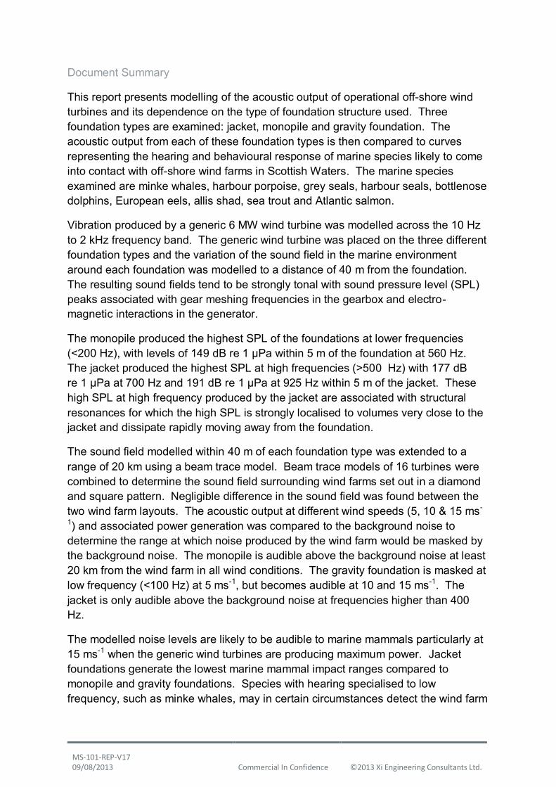
Document Summary
This report presents modelling of the acoustic output of operational off-shore wind turbines and its dependence on the type of foundation structure used. Three foundation types are examined: jacket, monopile and gravity foundation. The acoustic output from each of these foundation types is then compared to curves representing the hearing and behavioural response of marine species likely to come into contact with off-shore wind farms in Scottish Waters. The marine species examined are minke whales, harbour porpoise, grey seals, harbour seals, bottlenose dolphins, European eels, allis shad, sea trout and Atlantic salmon.
Vibration produced by a generic 6 MW wind turbine was modelled across the 10 Hz to 2 kHz frequency band. The generic wind turbine was placed on the three different foundation types and the variation of the sound field in the marine environment around each foundation was modelled to a distance of 40 m from the foundation. The resulting sound fields tend to be strongly tonal with sound pressure level (SPL) peaks associated with gear meshing frequencies in the gearbox and electro-magnetic interactions in the generator.
The monopile produced the highest SPL of the foundations at lower frequencies (<200 Hz), with levels of 149 dB re 1 µPa within 5 m of the foundation at 560 Hz. The jacket produced the highest SPL at high frequencies (>500 Hz) with 177 dB re 1 µPa at 700 Hz and 191 dB re 1 µPa at 925 Hz within 5 m of the jacket. These high SPL at high frequency produced by the jacket are associated with structural resonances for which the high SPL is strongly localised to volumes very close to the jacket and dissipate rapidly moving away from the foundation.
The sound field modelled within 40 m of each foundation type was extended to a range of 20 km using a beam trace model. Beam trace models of 16 turbines were combined to determine the sound field surrounding wind farms set out in a diamond and square pattern. Negligible difference in the sound field was found between the two wind farm layouts. The acoustic output at different wind speeds (5, 10 & 15 ms-
1) and associated power generation was compared to the background noise to determine the range at which noise produced by the wind farm would be masked by the background noise. The monopile is audible above the background noise at least 20 km from the wind farm in all wind conditions. The gravity foundation is masked at low frequency (<100 Hz) at 5 ms-1, but becomes audible at 10 and 15 ms-1. The jacket is only audible above the background noise at frequencies higher than 400 Hz.
The modelled noise levels are likely to be audible to marine mammals particularly at 15 ms-1 when the generic wind turbines are producing maximum power. Jacket foundations generate the lowest marine mammal impact ranges compared to monopile and gravity foundations. Species with hearing specialised to low frequency, such as minke whales, may in certain circumstances detect the wind farm

MS-101-REP-V17 09/08/2013 Commercial In Confidence ©2013 Xi Engineering Consultants Ltd.
at least 18 km away and are the species most likely to be affected by noise from operational wind turbines. Harbour seals, grey seals and bottlenose dolphins are not considered to be at risk of displacement by the operational wind farm modelled.
Atlantic salmon and European eels are able to detect the presence of monopiles at greater ranges than gravity bases, though this may not affect their behaviour. Allis shad and sea trout appear to not be able to detect noise produced by operational wind turbines except at close range (<100 m).
Authors
Dr Brett Marmo, Dr Iain Roberts, Dr Mark-Paul Buckingham - Xi Engineering Consultants
Dr Stephanie King, Dr Cormac Booth - SMRU Ltd
Matters relating to this document should be directed to:
Dr Kate Brookes
E: [email protected] Marine Scotland, Marine Laboratory, 375 Victoria Road, Aberdeen, AB11 9DB.

MS-101-REP-V17 09/08/2013 Commercial In Confidence ©2013 Xi Engineering Consultants Ltd.
Acknowledgements
Many thanks to all the individuals and companies that have assisted with this project. Specific thanks go to Repower, Ramboll and ARUP for their assistance with input data.
Thanks must also go to Dr Kate Brookes and Dr Ian Davies at Marine Scotland for all their hard work and assistance throughout.

MS-101-REP-V17 09/08/2013 Commercial In Confidence ©2013 Xi Engineering Consultants Ltd.
Contents
1 Introduction ............................................................................................................................................. 1
2 Technical background ............................................................................................................................... 1
2.1 Vibration and noise produced by wind turbines ............................................................................... 1
2.2 Vibration and underwater acoustics ................................................................................................. 3
2.3 Noise detection by marine species and background noise ................................................................ 6
2.4 Impacts of noise on marine mammals .............................................................................................. 8
2.4.1 Behavioural response .................................................................................................................. 9
2.5 Hearing sensitivity of marine mammals .......................................................................................... 10
2.5.1 Compiling species audiograms ................................................................................................... 11
2.6 Modelling overview ....................................................................................................................... 15
2.7 Determining zones of interest ........................................................................................................ 17
2.7.1 Audibility zones ......................................................................................................................... 17
2.7.2 Behavioural response zones....................................................................................................... 17
3 Near-field acoustic models ...................................................................................................................... 21
3.1 Modelling approach for comparison of offshore wind turbine foundations ..................................... 21
3.2 Geometry used for acoustic modelling ........................................................................................... 22
3.2.1 Wind turbine generator and tower ............................................................................................ 22
3.2.2 Gravity base .............................................................................................................................. 23
3.2.3 Jacket foundation ...................................................................................................................... 25
3.2.4 Monopile ................................................................................................................................... 26
3.2.5 Water acoustic domain .............................................................................................................. 26
3.2.6 Seabed domain .......................................................................................................................... 27
3.3 Material properties ........................................................................................................................ 27
3.4 Boundary conditions ...................................................................................................................... 29
3.4.1 Structural boundary conditions .................................................................................................. 30
3.4.2 Acoustic boundary conditions .................................................................................................... 33
3.4.3 Structural-acoustic interaction ................................................................................................... 34
3.5 Mesh parameters .......................................................................................................................... 35
3.6 Results ........................................................................................................................................... 37
3.6.1 Monopile results ....................................................................................................................... 38
3.6.2 Gravity results ........................................................................................................................... 41
3.6.3 Jacket results ............................................................................................................................. 43
3.6.4 Comparison of peak SPL values .................................................................................................. 46
4 Far-field acoustic model .......................................................................................................................... 48
4.1 Beam trace model ......................................................................................................................... 48

MS-101-REP-V17 09/08/2013 Commercial In Confidence ©2013 Xi Engineering Consultants Ltd.
4.2 Geometry and material properties ................................................................................................. 48
4.3 Results ........................................................................................................................................... 49
5 Effect of acoustic output on marine life ................................................................................................... 56
5.1 Marine mammals ........................................................................................................................... 56
5.1.1 Audibility zones ......................................................................................................................... 57
5.1.2 Behavioural response zones....................................................................................................... 62
5.2 Fish................................................................................................................................................ 66
6 Discussion ............................................................................................................................................... 72
6.1 Assumptions made and their effects on results .............................................................................. 72
6.1.1 Assumptions made in numerical modelling ................................................................................ 72
6.1.2 Assumptions affecting biological behaviour ............................................................................... 73
6.2 Performance of models relative to previous studies ....................................................................... 74
6.3 Comparison of foundation types .................................................................................................... 74
6.4 Operational noise from wind farms and its effect on the behaviour of marine species .................... 75
7 Conclusion .............................................................................................................................................. 77
8 Bibliography ........................................................................................................................................... 78
9 Appendix A – Document Register ............................................................................................................ 84
10 Appendix B – Far-field sound field ...................................................................................................... 86
11 Appendix C – m-weighted sound field ................................................................................................ 98
MS-101-REP-V17 Page 1 09/08/2013 Commercial In Confidence ©2013 Xi Engineering Consultants Ltd.
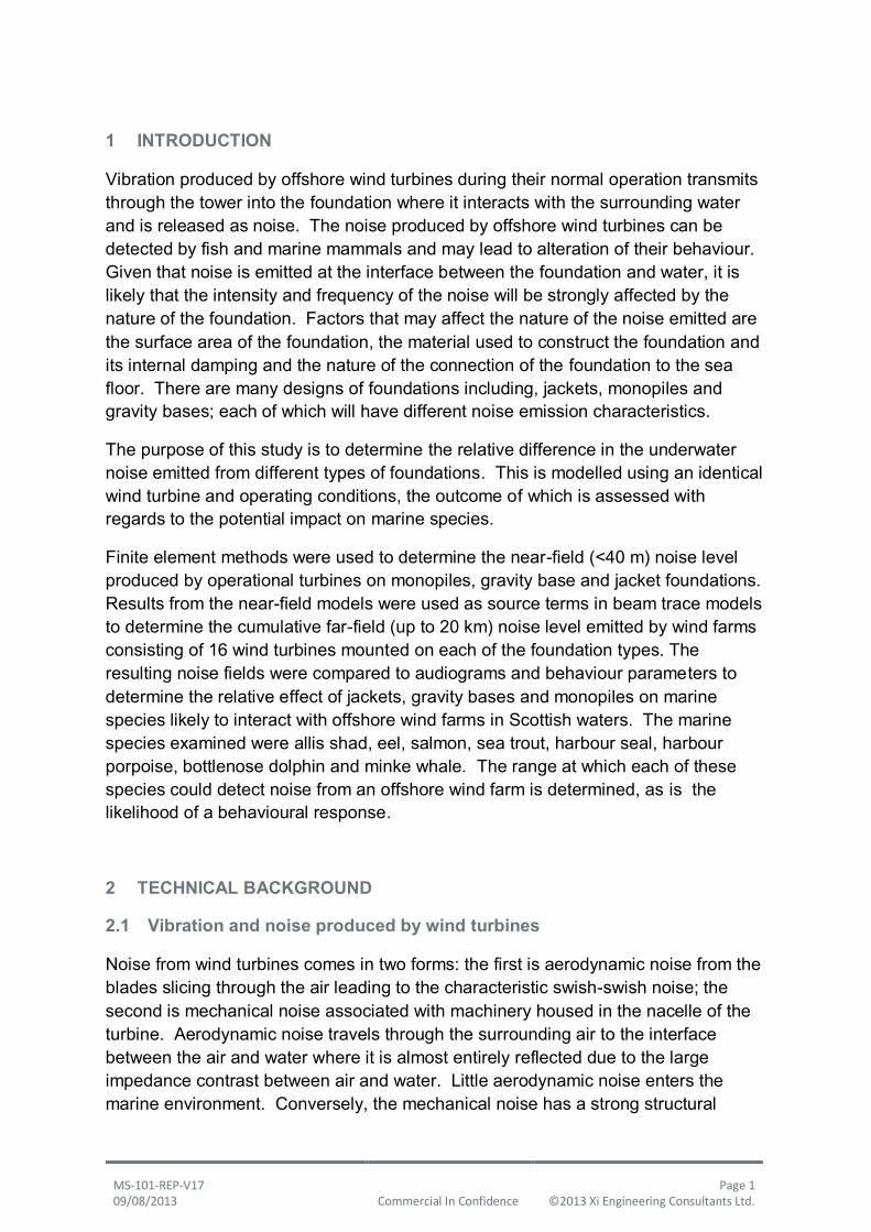
1 INTRODUCTION
Vibration produced by offshore wind turbines during their normal operation transmits through the tower into the foundation where it interacts with the surrounding water and is released as noise. The noise produced by offshore wind turbines can be detected by fish and marine mammals and may lead to alteration of their behaviour. Given that noise is emitted at the interface between the foundation and water, it is likely that the intensity and frequency of the noise will be strongly affected by the nature of the foundation. Factors that may affect the nature of the noise emitted are the surface area of the foundation, the material used to construct the foundation and its internal damping and the nature of the connection of the foundation to the sea floor. There are many designs of foundations including, jackets, monopiles and gravity bases; each of which will have different noise emission characteristics.
The purpose of this study is to determine the relative difference in the underwater noise emitted from different types of foundations. This is modelled using an identical wind turbine and operating conditions, the outcome of which is assessed with regards to the potential impact on marine species.
Finite element methods were used to determine the near-field (<40 m) noise level produced by operational turbines on monopiles, gravity base and jacket foundations. Results from the near-field models were used as source terms in beam trace models to determine the cumulative far-field (up to 20 km) noise level emitted by wind farms consisting of 16 wind turbines mounted on each of the foundation types. The resulting noise fields were compared to audiograms and behaviour parameters to determine the relative effect of jackets, gravity bases and monopiles on marine species likely to interact with offshore wind farms in Scottish waters. The marine species examined were allis shad, eel, salmon, sea trout, harbour seal, harbour porpoise, bottlenose dolphin and minke whale. The range at which each of these species could detect noise from an offshore wind farm is determined, as is the likelihood of a behavioural response.
2 TECHNICAL BACKGROUND
2.1 Vibration and noise produced by wind turbines
Noise from wind turbines comes in two forms: the first is aerodynamic noise from the blades slicing through the air leading to the characteristic swish-swish noise; the second is mechanical noise associated with machinery housed in the nacelle of the turbine. Aerodynamic noise travels through the surrounding air to the interface between the air and water where it is almost entirely reflected due to the large impedance contrast between air and water. Little aerodynamic noise enters the marine environment. Conversely, the mechanical noise has a strong structural

MS-101-REP-V17 Page 2 09/08/2013 Commercial In Confidence ©2013 Xi Engineering Consultants Ltd.
pathway between the drive train (where the vibration is created), through the nacelle support frame, tower, into the foundation and finally from the foundation into the surrounding water where it is released as noise. The great majority of noise in the marine environment due to wind turbines is therefore related to mechanical vibration in the drive train.
Mechanical vibrations in the drive trains of wind turbines are created by imbalances of the rotating components, the teeth in the gearbox coming into contact with each other (referred to as gear meshing), and electro-magnetic (E-M) interaction between the spinning poles and stationary stators in the generator. Each of these vibration sources occurs in discrete frequency bands related to the rotation speed of each component: the vibrations therefore tend to be tonal (as opposed to broad band). Rotational imbalances tend to occur at very low frequencies (< 50 Hz), while gear meshing and E-M interactions tend to occur at low to moderate frequencies (50 Hz to 2 kHz), Table 2-1. Other mechanical vibration produced by wind turbines during normal operation tend to be of a temporal nature with durations of seconds to tens of seconds. These include the pumping of hydraulic fluid, cooling systems and yawing of the nacelle followed by braking.
Table 2-1 Frequency bands likely to contain vibration tones produced in the drive train of wind turbines.
Frequency
Rotational imbalance of rotor 0.05 to 0.5 Hz
Rotational imbalance of high speed shaft between gearbox and generator 10 to 50 Hz
Gear teeth meshing 8 to 1000 Hz
Electro-magnetic interactions in the generator 50 to 2000 Hz
The amplitude of the vibration of a wind turbine and related noise emitted by the foundation is controlled by the size of the excitation force, the frequency of structural resonances and the level of damping in the structure. The magnitude of the excitation of the drive train is related to the torque acting on the rotor, which is dependent on the wind speed. The amplitude of vibration of the turbine increases with the square of wind speed at the hub height. It is likely, therefore, that the noise emitted by the foundation will also rise with wind speed.
Mechanical noise can be amplified by structural resonances within the wind turbine. Structural resonances are the harmonic frequencies at which a structure vibrates when excited by a discrete event (e.g. the frequency a bell rings when struck). When an excitation frequency such as gear meshing has the same frequency as a structural resonance, the amplitude of the vibration is amplified, sometime dramatically. This becomes important in the event of frequency matching between

MS-101-REP-V17 Page 3 09/08/2013 Commercial In Confidence ©2013 Xi Engineering Consultants Ltd.
an excitation frequency in the drive train and a resonance in the foundation as the noise emitted into the marine environment will be significantly amplified.
Understanding structural resonances is also important because resonances can be excited by multiples of excitation frequencies. For instance, a resonant mode in the steel surface of the tower at 600 Hz can be excited by a gear meshing frequency of 200 Hz. In this example the resonance coincides with the third multiple of the gear meshing (3 × 200 Hz = 600 Hz). Structural resonances can therefore produce vibration and related noise at frequencies that would not otherwise have been excited.
All structures contain some level of internal damping. Damping is the dissipation of vibration energy via processes like heat loss and has the effect of reducing the amplitude of vibration. In general, steel structures such as jackets have less damping than structures built from granular materials such as concrete foundations. The level of internal damping will therefore affect the noise emitted by different types of foundations. Damping may also be increased over time by biofouling, where the encrusted organisms begin to act as a granular aggregate with high internal friction.
2.2 Vibration and underwater acoustics
At the interface between the foundation and water, the vibration of the foundation oscillates water molecules to produce a pressure wave which radiates away from the foundation as sound. As the sound propagates away from the foundation its intensity is reduced with distance due to geometric spreading and absorption. Water absorbs high frequency sound more quickly than low frequencies; low frequency sound therefore propagates further. At the sea surface the sound is almost perfectly reflected by the high impedance contrast between water and air, though some sound may be scattered by surface waves or absorbed by near-surface air bubbles. At the seabed sound is also reflected and scattered, though its behaviour is more difficult to predict than at the surface due to the seabed’s variable acoustic properties (soft sediment to hard rock) and internal layering of material with different densities and sound speeds.
Several underwater acoustic measurements of offshore wind turbines have been carried out (Westerberg 1994, Degn 2000, Ingemansson Technology 2003, Betke et al 2004, Thomsen 2006, Nedwell 2011). Measurements recorded to date have been of turbines with different design parameters, such as foundation type, water depth, turbine size, sediment type and wind speeds - making direct comparisons difficult. However, noise related to off-shore wind turbines have common features; specifically, the sound intensity is dominated by pure tones likely to originate from rotating machinery in the nacelle with frequencies mostly below 700 Hz.
MS-101-REP-V17 Page 4 09/08/2013 Commercial In Confidence ©2013 Xi Engineering Consultants Ltd.
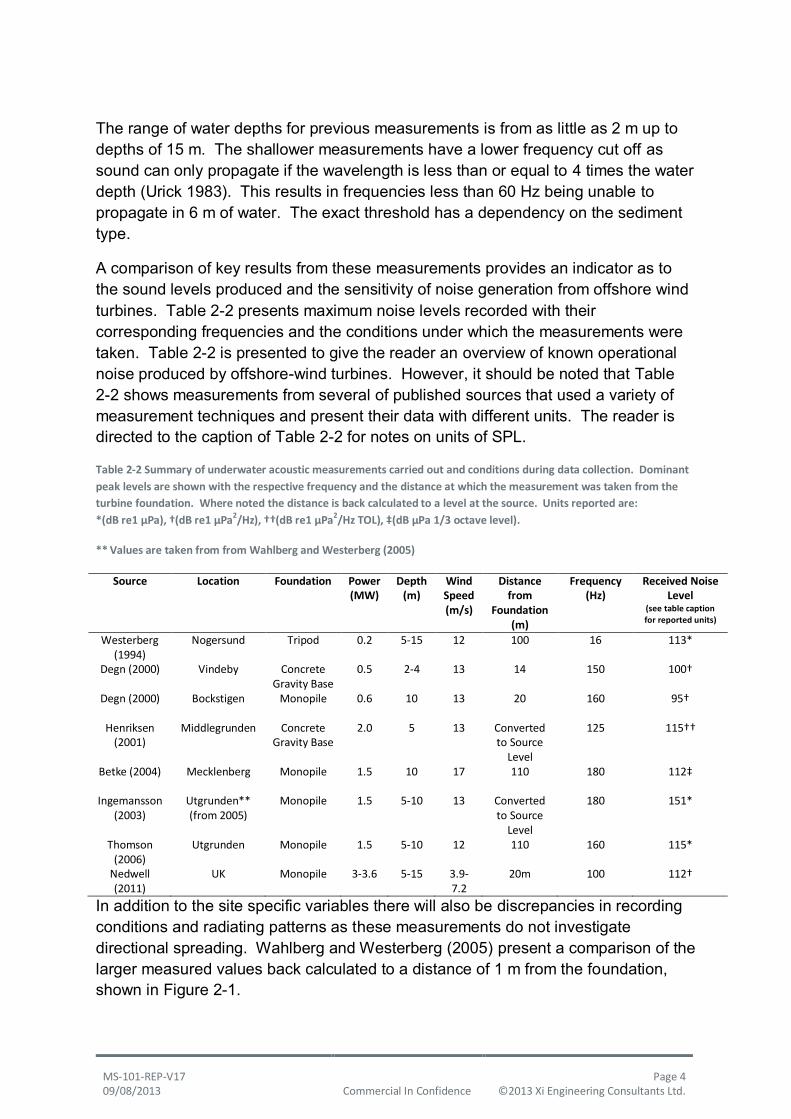
The range of water depths for previous measurements is from as little as 2 m up to depths of 15 m. The shallower measurements have a lower frequency cut off as sound can only propagate if the wavelength is less than or equal to 4 times the water depth (Urick 1983). This results in frequencies less than 60 Hz being unable to propagate in 6 m of water. The exact threshold has a dependency on the sediment type.
A comparison of key results from these measurements provides an indicator as to the sound levels produced and the sensitivity of noise generation from offshore wind turbines. Table 2-2 presents maximum noise levels recorded with their corresponding frequencies and the conditions under which the measurements were taken. Table 2-2 is presented to give the reader an overview of known operational noise produced by offshore-wind turbines. However, it should be noted that Table 2-2 shows measurements from several of published sources that used a variety of measurement techniques and present their data with different units. The reader is directed to the caption of Table 2-2 for notes on units of SPL.
Table 2-2 Summary of underwater acoustic measurements carried out and conditions during data collection. Dominant
peak levels are shown with the respective frequency and the distance at which the measurement was taken from the
turbine foundation. Where noted the distance is back calculated to a level at the source. Units reported are:
*(dB re1 µPa), †(dB re1 µPa2/Hz), ††(dB re1 µPa2/Hz TOL), ‡(dB µPa 1/3 octave level).
** Values are taken from from Wahlberg and Westerberg (2005)
Source Location Foundation Power (MW)
Depth (m)
Wind Speed (m/s)
Distance from
Foundation (m)
Frequency (Hz)
Received Noise Level
(see table caption for reported units)
Westerberg (1994)
Nogersund Tripod 0.2 5-15 12 100 16 113*
Degn (2000) Vindeby Concrete Gravity Base
0.5 2-4 13 14 150 100†
Degn (2000) Bockstigen Monopile 0.6 10 13 20 160 95†
Henriksen (2001)
Middlegrunden Concrete Gravity Base
2.0 5 13 Converted to Source
Level
125 115††
Betke (2004) Mecklenberg Monopile 1.5 10 17 110 180 112‡
Ingemansson (2003)
Utgrunden** (from 2005)
Monopile 1.5 5-10 13 Converted to Source
Level
180 151*
Thomson (2006)
Utgrunden Monopile 1.5 5-10 12 110 160 115*
Nedwell (2011)
UK Monopile 3-3.6 5-15 3.9-7.2
20m 100 112†
In addition to the site specific variables there will also be discrepancies in recording conditions and radiating patterns as these measurements do not investigate directional spreading. Wahlberg and Westerberg (2005) present a comparison of the larger measured values back calculated to a distance of 1 m from the foundation, shown in Figure 2-1.

MS-101-REP-V17 Page 5 09/08/2013 Commercial In Confidence ©2013 Xi Engineering Consultants Ltd.
Figure 2-1 Wahlberg and Westerberg (2005) present a summary of source-level measurements of underwater noise
generated by turbines. The measurements were caried out by Westerberg (1994: Nogersund), Degn (2000: Bockstigen 8
ms–1 and Vindeby), Fristedt et al. (2001: Bockstigen 5 ms–1) and Ingemansson (2003: Utgrunden). Noise level:
background noise level measured by Piggott (1964) in 40 to 50 m water depth. The properties and conditions of
recording are as in Table 2-2. The noise levels have been back calculated by Wahlberg and Westerberg (2005) to a
distance of 1 m for comparison.
The highest levels presented by Wahlberg and Westerberg (2005) were achieved by Ingemansson (2003) with 151 dB re1 µPa at 180 Hz at a back calculated distance of 1 m from the foundation. Madsen (2006) expand on the review of Wahlberg and Westerberg (2005) summarising that the tonal peaks seen below 1 kHz are likely to be linked to the mechanical properties of the turbine with no direct measurements of source tonal levels exceeding 145 dB re 1µPa (RMS). In addition, Madsen (2006) reviewed that measured levels drop below 120 dB re 1µPa (RMS) at 100m. However measurements to date do not account for directional components or cumulative effects of multiple turbines.

MS-101-REP-V17 Page 6 09/08/2013 Commercial In Confidence ©2013 Xi Engineering Consultants Ltd.
2.3 Noise detection by marine species and background noise
Marine fauna exposed to anthropogenic sound may experience detrimental effects that include physical injury, behavioural disturbance and displacement, masking of biologically important signals, and other indirect effects. These are defined by the proximity of the animal to the sound source, the sound level received by the animal, the hearing sensitivity and acoustic characteristics of the vocalisations of the animal, and the acoustic characteristics of the anthropogenic noise.
The key potential impacts of operational turbine noise on marine species are:
Disturbance as a result of underwater noise arising from operational offshore wind turbines.
Potential longer term avoidance of the development area by marine mammals Potential reduction of the feeding resource due to the effects of noise,
vibration, and habitat disturbance on important prey species
Assessment of the likely extent and significance of such impacts should be quantitative wherever possible and all uncertainties explicitly included. Marine species hearing sensitivities cover a broad frequency range and as such the same sound source may elicit different behavioural and physiological effects in different species. In addition, within-species responses may vary depending on individual traits of exposed animals and the context in which they are exposed. Nevertheless, based on previous published studies and established noise threshold recommendations, generalised predictions of how individual species may be impacted by certain noise sources are possible.
The frequency band over which different species can sense noise varies greatly (Table 2-3). In general fish sense noise in the 10s to 100s of Hz range, though some clupeiform fish including shad may hear into the 100s kHz range. Marine mammals such as seals, dolphins and whales are capable of hearing noise between 10s of Hz to 100s of kHz. Wind turbines produce vibration and related noise between 0.5 Hz to 2 kHz (Table 2-1) which overlaps frequency bands that are detectable by species living in Scottish waters (Table 2-3).
While marine species are capable of hearing noise from wind turbines, in many cases this will be masked by the background noise of the ocean. The ocean is inherently a noisy place with background noise contributed by wind interaction with the surface, rain, industrial activity and shipping, explosions and earthquakes and biological activity. At some range from a wind turbine the noise produced will be less than the background noise at which point marine species will no longer be able to detect it. Of particular importance in relation to wind turbines is the relationship between wind speed and noise production. As has been noted above, the vibration and noise produced by wind turbines increases with wind speed. There is a similar relationship between wind speed and background noise (Urick, 1983). Thus, while

MS-101-REP-V17 Page 7 09/08/2013 Commercial In Confidence ©2013 Xi Engineering Consultants Ltd.
wind turbine noise increases with wind speed, so too does the masking effect of background noise, Figure 2-2. For the purpose of this study a worst-case scenario is taken where the lowest applicable background noise is used so that masking effects are minimised. Thus, the background noise is taken as the lowest SPL associated with low frequency shallow water noise from 0 to ~100 Hz (lower boundary of the brown field in Figure 2-2) combined with the SPL associated with the relevant sea state conditions at higher frequency (>100 Hz). The relevant sea states to wind speed are taken as: sea state 2 for wind speeds of 5 ms-1; sea state 4 for wind speeds of 10 ms-1 and; sea state 6 for wind speeds of 15 ms-1. Continuing to follow the worst-case for masking; temporal increases in SPL associated with shipping have been excluded from the background noise.
Table 2-3 Approximate sound detection frequency range for some species in Scottish waters.
Species Hearing range Reference
Allis shad 10 Hz to 180 kHz (Mann, et al. 2001)
European eel 10 to 300 Hz (Jenko, et al. 1989)
Salmon 32 to 400 Hz (Hawkins and Myrberg 1983)
Sea trout 100 to 1000 Hz (Horodysky, et al. 2008)
Minke whales 7 Hz to 22 kHz (Southall et al. 2007)
Bottlenose dolphin 150 Hz to 160 kHz (Southall et al. 2007)
Harbour porpoise 200 Hz to 180 kHz (Southall et al. 2007)
Grey seal 75 Hz to 75 kHz (Southall et al. 2007)
Harbour seal 75 Hz to 75 kHz (Southall et al. 2007)

MS-101-REP-V17 Page 8 09/08/2013 Commercial In Confidence ©2013 Xi Engineering Consultants Ltd.
Figure 2-2 Wenz curve showing typical sound levels in the ocean (Wenz 1962) with sound level in units relative to 1μPa.
2.4 Impacts of noise on marine mammals
Marine mammals spend most, or all, of their lives at sea, and for the majority of that time they are submerged. Sound propagates efficiently through water and marine mammals rely on the use of sound to communicate with conspecifics, for predator avoidance, to locate and capture prey, mate selection and social interactions (Akamatsu et al. 1994; Au et al. 2004; Goodson and Sturtivant 1996; Hafner et al. 1979; Hastie et al. 2006; Janik 2000; Janik 2009; Madsen et al. 2005a; Madsen et al. 2005b; Rendell and Whitehead 2004; Schulz et al. 2008). Coupled with this, they have an acute sense of hearing with a high sensitivity over a wide frequency range (Nedwell et al. 2004; Richardson et al. 1995; Southall et al. 2007). This reliance on

MS-101-REP-V17 Page 9 09/08/2013 Commercial In Confidence ©2013 Xi Engineering Consultants Ltd.
sound in their general ecology makes marine mammals particularly vulnerable to the effects of underwater noise.
Any anthropogenic noise could impact a marine mammal if the sound falls within its audible range; noise disturbance can have a range of effects depending on the sound type or source level. Loud, intense noise sources such as explosions have the potential to cause lethal physical non-auditory injury to marine mammals, while other noise sources can cause auditory damage, elicit behavioural responses (e.g. displacement and/or habitat exclusion), induces stress and/or mask biologically important signals (Richardson et al. 1995).
Given the relatively low noise levels emitted from operational wind turbines, it is not likely that sound levels are high enough to cause auditory injury beyond a few metres of the device and only if animals remain there for extended periods of time. We therefore only consider the impact of noise from marine operational wind turbines on the behavioural response of five priority species of marine mammal:
Harbour porpoise (Phocoena phocoena) Bottlenose dolphin (Tursiops truncatus) Minke whale (Balaenoptera acutorostrata) Harbour seal (Phoca vitulina) Grey seal (Halichoerus grypus)
2.4.1 Behavioural response
The introduction of noise into the underwater environment may impair an animal’s ability to detect calls or may disrupt its normal behaviour in some way. Noise impacts can be thought of in terms of 4 zones of influence (Richardson et al. 1995). The zone of audibility is the range at which animals can only just detect the anthropogenic sound source. The zone of masking is the range at which the sound exposure interferes with the signals produced by the animal, at a given frequency, and thus lowers the probability of the animal’s signal being detected. This means the distances over which animals can communicate will be greatly reduced. The zone of responsiveness is smaller and is the impact range around the sound source where animals are expected to show physiological or behavioural responses to the sound. The zone of injury is the smallest zone but potentially with the highest impact. This is defined as the range at which the received sound levels are high enough to induce either direct physical injury or loss of hearing sensitivity (hearing damage).
The likelihood of an animal experiencing one or more of these effects is defined by the spatial relationship of the receiver and the sound source, the hearing sensitivity and acoustic characteristics of the vocalisations of the receiver, and the acoustic

MS-101-REP-V17 Page 10 09/08/2013 Commercial In Confidence ©2013 Xi Engineering Consultants Ltd.
characteristics of the anthropogenic noise. Consequently, for many sound sources, responses are poorly described and predictions of potential effects can be challenging. Nevertheless, based on previous published studies and noise threshold recommendations, generalised predictions of how individual species may be impacted by certain noise sources are possible.
While the physical process of detecting or being damaged by a sound can be predicted from a combination of empirical studies and acoustic models, this is generally not the case for behavioural responses. The behavioural response of animals to sound appears to be influenced by a number of factors including food
motivation, the context of exposure, and the animal’s previous exposure history. This means that the way in which an individual responds to sound can vary between both individuals and sound exposure events.
2.5 Hearing sensitivity of marine mammals
The hearing ability of marine mammals is commonly described using audiograms; this is a plot of the hearing sensitivity of a species at different frequencies, which indicates the range of frequencies detectable by a species and can highlight where hearing is most sensitive. The hearing threshold can be defined as the received sound level in the vicinity of the ear that is just audible to an animal. Hearing thresholds depend on the frequency of the sounds and can vary strongly across species. An audiogram displays hearing threshold as a function of frequency. A lower sound pressure level value on an audiogram display reflects a low hearing threshold at a given frequency and hence a high auditory sensitivity. Audiograms for mammals are typically V- or U-shaped reflecting the fact that hearing sensitivity declines towards the edge of the hearing range (i.e. at both ends of the V/U-shape).
Audiograms are typically derived experimentally and can be based on behavioural or electrophysiological responses (AEP/ABR) to sound stimuli. Both approaches are considered robust methods for collecting audiogram data. However, it is unclear how the AEP measurements compare with audiograms derived from behavioural methods. Some studies have indicated that behavioural hearing thresholds are generally lower (i.e. more sensitive) than AEP/ABR thresholds (e.g. Szymanski, et al. 1999; Yuen, et al. 2005). It is also important to consider that audiograms may be generated using different stimuli and therefore not all audiograms may be directly comparable. However, given the paucity of audiogram data for marine mammal species- considering the suitability of all available data is important.
Studies on the hearing sensitivity in marine mammals are usually carried out on captive animals and as a consequence, audiograms have not been measured for the majority of species. Furthermore, audiograms have been calculated for a limited number of individual animals of each species and consequently may not capture the

MS-101-REP-V17 Page 11 09/08/2013 Commercial In Confidence ©2013 Xi Engineering Consultants Ltd.
variation in auditory ranges or most sensitive frequencies across the entire species. However, despite the lack of data on the hearing sensitivities of many marine mammals at the species level, it is possible to make some generalisations about hearing across higher taxonomic levels.
2.5.1 Compiling species audiograms
In compiling audiogram data for the species of interest, where possible only data collected for that species were used in the study. However, due to the paucity of audiogram data available it was necessary to sometimes use data from other homologous species to build complete audiograms given the nature of noise sources being considered here (e.g. low frequency continuous noise). Studies where the absolute values from hearing sensitivity experiments were presented were used. In many studies, a visual plot of the audiogram was shown, but no empirical data presented. However, many of these plots were reviewed in the generation of ‘composite audiograms’ to ensure important studies/findings were not being overlooked.
For each species, once the data had been assimilated, an assessment was made of how many studies and individual study animals a suitable audiogram could be compiled from. For each species a composite ‘most sensitive animal’ audiogram was constructed. This was a precautionary approach to try to avoid an underestimation of the potential impact zones.
2.5.1.1 Bottlenose dolphin In general, small- to medium-sized odontocetes (e.g. dolphin species) have good hearing across a broad range of frequencies (4-100 kHz) and are most sensitive to sounds above 10 kHz (Richardson et al. 1995), but can hear sounds below this level (Figure 2-3). Available studies of bottlenose dolphin hearing thresholds only went down to 8 kHz (Houser & Finneran, 2006; Popov, et al. 2007; Houser, et al. 2008) and so data from beluga whales (from White, et al., 1978) were used as a proxy for bottlenose dolphins below this frequency.

MS-101-REP-V17 Page 12 09/08/2013 Commercial In Confidence ©2013 Xi Engineering Consultants Ltd.
Figure 2-3 - Audiograms for bottlenose dolphin and the composite audiogram derived and used here. AEP indicates that
auditory evoked potentials or auditory brainstem responses were used to calculate the audiograms.
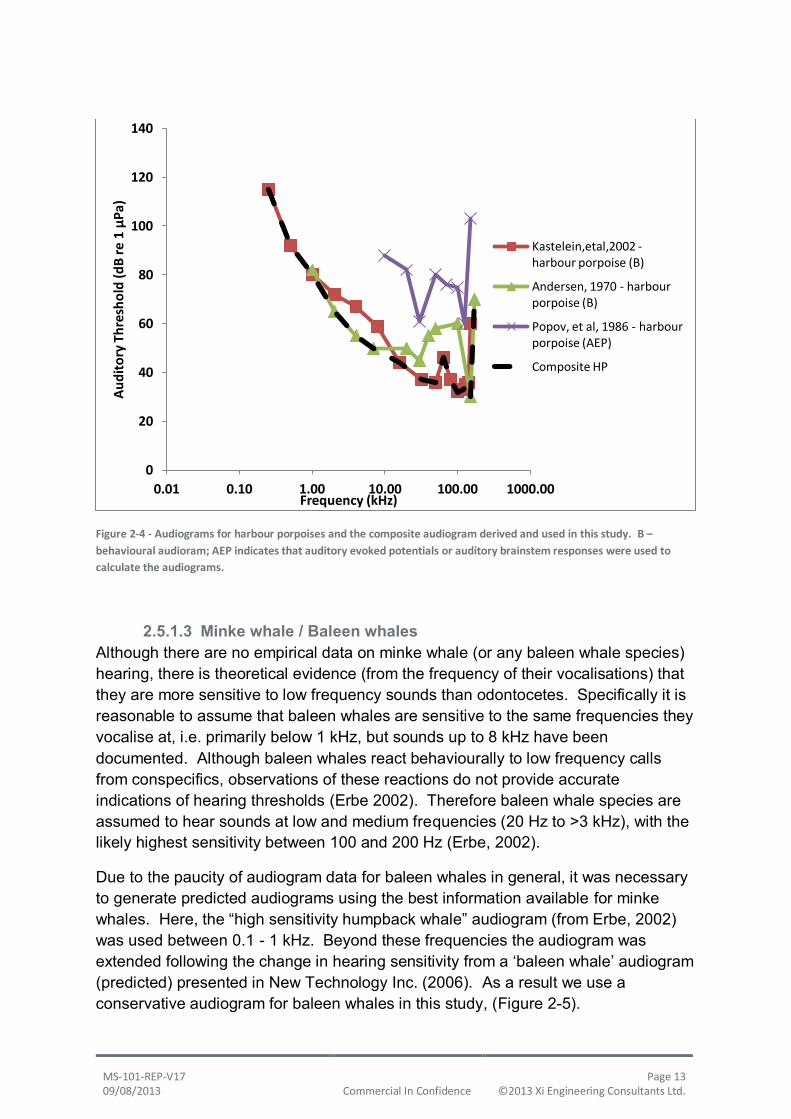
2.5.1.2 Harbour porpoise Harbour porpoises echolocate at high frequencies (125-150 kHz) and have excellent mid-high frequency hearing (Goodson & Sturtivant, 2002; Kastelein, et al., 2002). The composite audiogram for the species was constructed from behavioural and AEP studies (with animals more sensitive in the behavioural audiograms) and have good hearing down to ~4 kHz (Andersen, 1970; Kastelein, et al. 2002) (Figure 2-4). Below this frequency the species hearing capability is predicted to be low.
0
20
40
60
80
100
120
140
160
0.01 0.1 1 10 100 1000
Au
dit
ory
Th
resh
old
(d
B r
e 1
µP
a)
Frequency (kHz)
Popov, et al. 2007 - bottlenose dolphin (AEP)
Houser, et al., 2008 - bottlenose dolphin (AEP)
Houser & Finneran, 2006 - bottlenose dolphin (AEP)
Composite BND
MS-101-REP-V17 Page 13 09/08/2013 Commercial In Confidence ©2013 Xi Engineering Consultants Ltd.
Figure 2-4 - Audiograms for harbour porpoises and the composite audiogram derived and used in this study. B –
behavioural audioram; AEP indicates that auditory evoked potentials or auditory brainstem responses were used to
calculate the audiograms.
2.5.1.3 Minke whale / Baleen whales Although there are no empirical data on minke whale (or any baleen whale species) hearing, there is theoretical evidence (from the frequency of their vocalisations) that they are more sensitive to low frequency sounds than odontocetes. Specifically it is reasonable to assume that baleen whales are sensitive to the same frequencies they vocalise at, i.e. primarily below 1 kHz, but sounds up to 8 kHz have been documented. Although baleen whales react behaviourally to low frequency calls from conspecifics, observations of these reactions do not provide accurate indications of hearing thresholds (Erbe 2002). Therefore baleen whale species are assumed to hear sounds at low and medium frequencies (20 Hz to >3 kHz), with the likely highest sensitivity between 100 and 200 Hz (Erbe, 2002).
Due to the paucity of audiogram data for baleen whales in general, it was necessary to generate predicted audiograms using the best information available for minke whales. Here, the “high sensitivity humpback whale” audiogram (from Erbe, 2002) was used between 0.1 - 1 kHz. Beyond these frequencies the audiogram was extended following the change in hearing sensitivity from a ‘baleen whale’ audiogram (predicted) presented in New Technology Inc. (2006). As a result we use a conservative audiogram for baleen whales in this study, (Figure 2-5).
0
20
40
60
80
100
120
140
0.01 0.10 1.00 10.00 100.00 1000.00
Au
dit
ory
Th
resh
old
(d
B r
e 1
µP
a)
Frequency (kHz)
Kastelein,etal,2002 - harbour porpoise (B)
Andersen, 1970 - harbour porpoise (B)
Popov, et al, 1986 - harbour porpoise (AEP)
Composite HP

MS-101-REP-V17 Page 14 09/08/2013 Commercial In Confidence ©2013 Xi Engineering Consultants Ltd.
Figure 2-5 - Predicted audiogram data for baleen whales and the composite minke whale audiogram used in this study.
Two audiograms were taken from Erbe, 2002 – one predicted ‘high sensitivity’ and one ‘low sensitivity’. The more
sensitive of the two was chosen as a more precautionary approach.
2.5.1.4 Seals (Grey and Harbour seals) Seals do not echolocate but do utilise acoustic communication both in and out of water, and are considered to hear best at frequencies between 1-30 kHz (Richardson et al. 1995) (Figure 2-6). Seals have markedly different hearing capabilities in air and underwater (Kastak and Schusterman 1998), and studies have shown that pinnipeds are sensitive to a broader range of sound frequencies in water than in air (Southall et al. 2007). In-air sound exposure is not considered within the scope of this project and so aerial hearing abilities will not be considered further.
In this study, audiogram data compiled for grey and harbour seals were used to generate a single composite audiogram for the species. Data from these species (Ridgeway & Joyce, 1975; Kastelein, et al. 2009; Götz & Janik, 2010), and other phocid seals found in the northeast Atlantic (e.g. harp seal – Terhune & Ronald, 1972), were also considered when compiling the seal composite audiogram (Figure 2-6).
0
20
40
60
80
100
120
140
160
0.001 0.01 0.1 1 10 100
Au
dit
ory
Th
resh
old
(d
B r
e 1
µP
a)
Frequency (kHz)
New Tech Inc 2006
Erbe High Sens
Erbe Low Sens
Composite Audiogram

MS-101-REP-V17 Page 15 09/08/2013 Commercial In Confidence ©2013 Xi Engineering Consultants Ltd.
Figure 2-6 - Pinniped audiograms used to derive composite audiogram used in this study. B – behavioural audioram; AEP
indicates that auditory evoked potentials or auditory brainstem responses were used to calculate the audiograms.
2.6 Modelling overview
Xi Engineering Consultants have developed a structural-acoustic interaction model using a finite element method that has successfully modelled air-borne noise produced by onshore wind turbines (Marmo & Caruthers 2011, Marmo 2011) and marine noise produced by tidal stream generators (Caruthers & Marmo, 2011). These models were developed using the commercially available modelling package COMSOL Multiphysics (Comsol) and have been validated using field evidence. Here three different foundation types have been modelled to determine the effect that different foundations have on the noise propagation from wind turbines into the marine environments.
1. Jacket with pin piles connection to the seabed 2. Monopile piled into the seabed with a transition piece 3. Gravity base structure sitting on the seabed
There is a complex range of variables that will affect the noise radiating from the foundations. These include:
Vibration spectra produced by the wind turbine (frequency and amplitude)
0
20
40
60
80
100
120
140
160
180
0.01 0.1 1 10 100 1000
Au
dit
ory
Th
resh
old
(d
B r
e 1
µP
a)
Frequency (kHz)
Grey seal - Ridgeway & Joyce (1975) (AEP)
Harbour seal (composite from Gotz and Janik, 2010)
Harp seal (Terhune & Ronald, 1972) (B)
Harbour seal (Kastelein, et al., 2009) (B)
Composite seal

MS-101-REP-V17 Page 16 09/08/2013 Commercial In Confidence ©2013 Xi Engineering Consultants Ltd.
Wind speed Water depth Seabed sediment type and thickness Biofouling
In practise, the selection of foundation type and its design is based on a range of environmental and economic factors. Environment factors overlap with those that effect noise radiation, such as water depth and seabed type. It may not make sense to use a jacket in shallow water nor a gravity base in deep water. The purpose of the proposed work is to compare the effect of foundation type on noise, so each foundation will be modelled using the same input forces from the wind turbine and same environmental conditions with the exception of water depth. Both the jacket and gravity base can be modelled in the deeper 50 m of sea water, whereas the monopile is generally not used in depths exceeding 30 m and so will use this shallower level with all other variables remaining unchanged. Also, biofouling is assumed to not have occurred to simplify the model.
The process of modelling for this project is two-fold. Firstly a near-field model of a single turbine-foundation system is formed where the structural - acoustic interaction is quantified. The output of this is the soundscape radiating from single turbines, repeated for each of the three different foundations. The sound field consists of spatial variation of sound intensity and its frequency and characterises the foundations source term up to 30 m.
The near-field source term is then used as the input for a far-field acoustic model. Maintaining the radial and frequency dependency signal produced from the structural - acoustic interaction the source term is applied to multiple locations forming wind farm configurations, (Figure 4-1):
1) Diamond 2) Square
This enables the far-field to be investigated using a beam trace model, including the cumulative effect from multiple sources. The 3-dimensional acoustic far-field soundscape produced is compared to background noise, accounting for the sea state under relevant environmental conditions, so that the range at which the turbine noise is masked by background noise can be determined. Audiograms for the chosen species, Table 2-3, are then imposed onto the modelled sound field and detection levels for the relevant frequencies are ascertained. The potential effect of noise output from off-shore turbines on marine species were examine in three zones of interest:
1. Audibility zone 2. Behaviour response zone 3. Auditory injury zone

MS-101-REP-V17 Page 17 09/08/2013 Commercial In Confidence ©2013 Xi Engineering Consultants Ltd.
The definitions of these zones and the parameters used to examine them are described below.
2.7 Determining zones of interest
2.7.1 Audibility zones
The range out to which the noise generated by operational wind turbines was audible to the species of interest was assessed. The sound field produced by each wind farm can be examined to determine where the sound pressure level (SPL) is equal to or greater than the hearing threshold of each species for any given frequency. The audiograms described above were applied in this way to the modelled far-field sound field and the maximum range at which marine mammals could hear the wind farm determined as a function of frequency. It is assumed that if the background noise exceeds the SPL produced by the wind farm that the noise from the farm is masked and cannot be detected by marine species. Thus, the maximum range at which the wind farm is audible to marine species is less than or equal to the range shown, depending on the hearing sensitivity of the species in question.
2.7.2 Behavioural response zones
The observed variability in the behavioural response of marine mammals to sound exposure makes it difficult to identify an exposure threshold at which animals will respond. Instead behavioural response should be thought of as probabilistic and is best described with dose-response relationships between the onset of a behavioural response and the received sound level. Although the development of dose-response curves for marine mammal response to sound exposure is currently underway these curves are not yet available and as there are still discussions over the best metric for assessing behavioural impact zones, we present the range of metrics that are currently favoured by the scientific community:
Audiogram + Sensation levels Weighted SPLs
o M-weighting o Reverse audiogram weighting
Table 2-4 - Sensation levels and behavioural response sound pressure levels (SPL) (RMS) for each of the species/groups.
The behavioural response SPLs correspond to the sound levels at which 10%, 50% and 90% (see section 2.7.2.2) of
animals that experience the SPL are predicted to respond.

MS-101-REP-V17 Page 18 09/08/2013 Commercial In Confidence ©2013 Xi Engineering Consultants Ltd.
Sensation level Behavioural response SPLs (RMS) Auditory Injury (SEL)
Species Lower Upper 10% 50% 90% PTS
Seals 451 592 -- 1352 1442 2034
HP 493 -- 904 1204 1404 2154
BND 49 -- 1204 1404 1604 2154
MW 49 -- 1204 1404 1604 2154 1
Kastelein et al. 2006; 2 Götz & Janik 2010;
3 Kastelein et al. 2005;
4 adapted from
Southall et al. 2007.
2.7.2.1 Audiogram and sensation level Behavioural response zones were calculated using sensation level thresholds. The sensation level is a pressure level in dB by which a sound exceeds the hearing threshold. Equal sensation levels can be expected to roughly cause similar loudness perception. Although there are limited data on which sensation levels generate a behavioural response in marine mammals, there are a few studies that do provide empirical data for marine mammal response to sound exposure. Sensation levels for harbour porpoise response to underwater data transmission sounds were 49 dB re 1 µPa at low frequencies (Kastelein, et al. 2005), sensation levels for grey seal response to ‘500/530 square’ noise stimuli, a ‘rough’ sound perceived to be unpleasant by humans, were 59 dB re 1 µPa (Götz and Janik, 2010), and sensation levels for harbour seal response to underwater data transmission sounds were 45 dB re 1 µPa (Kastelein et al. 2006).
For the purpose of this assessment the sensation levels described above were used to predict behavioural response ranges for pinnipeds and harbour porpoise. The sensation levels for grey seals and harbour seals were combined and treated as an upper and lower sensation level (Table 2-4). Due to the lack of empirical data for bottlenose dolphins and minke whales, the harbour porpoise sensation level was used to predict behavioural response ranges for all cetaceans as a conservative approach.
For each species, the predicted SPLs were compared to the composite audiograms to calculate the sensation level. To determine the sensation level that may result in a behavioural response in seals the sensation parameters were added to the sound level integrated across the two neighbouring one-third octave bands either side of the band of interest. In the case of cetaceans the sensation level was found by adding the sensation parameters to the SPL integrated across the four neighbouring bands on the dominant side of the band of interest.
If the sensation level was equal or higher to the sensation threshold presented in Table 2-4 then a behavioural response is predicted to occur.

MS-101-REP-V17 Page 19 09/08/2013 Commercial In Confidence ©2013 Xi Engineering Consultants Ltd.
2.7.2.2 Weighted sound pressure level (m-weighting and reversed audiogram)
The most complete review of behavioural responses by marine mammals to date is found in Southall et al (2007). Southall and colleagues reviewed available studies on behavioural responses to sound exposure in cetaceans and pinnipeds and proposed a severity scaling on which the level of the response could be measured. They did not, however, present explicit step-function thresholds for behavioural response. Animals may exhibit behavioural responses of varying magnitudes to noise exposure depending on species, sound type, exposure level and other contextual factors. Southall et al. (2007) provides a range of sound levels at which animals have shown to exhibit a behavioural response. Given that behavioural response should be thought of as probabilistic and is best described with a dose-response relationship that describes the proportion of animals that may expected to respond to a given sound level, for the purpose of this assessment we apply a probabilistic metric at which 10%, 50% and 90% of individuals exposed to these range of sound levels are predicted to show a behavioural response. We used Southall et al. (2007) and more recent literature to ascertain what sound levels had resulted in a behavioural response for each of the marine mammal hearing groups.
1. Pinnipeds appeared to exhibit only mild avoidance responses to non-pulse (continuous) noise at received levels between 90 and 140 dB re 1µPa. However, Götz & Janik (2010) showed sustained avoidance responses in wild grey seals at received levels of 135-144 dB re 1µPa; for the purposes of this assessment, the range at which these levels (135-144 dB re 1µPa) were exceeded were used as a threshold where 50% and 90% of animals respectively were predicted to show a strong behavioural response.
2. Harbour porpoise appear to be relatively sensitive to noise levels as low as 90-120 dB re 1µPa (Southall et al. 2007) although there also appears to be considerable variation between individuals. For the purpose of this assessment we have chosen 90 dB and 120 dB as a step-function threshold where 10% and 50% of animals respectively are predicted to show a behavioural response. However, data also suggests that harbour porpoise and other high-frequency cetaceans are likely to show a behavioural response when exposed to noise at much lower received levels than other species. Therefore, in contrast to other species, we use a lower level of 140 dB as a threshold where 90% of harbour porpoise are predicted to behaviourally respond.
3. Bottlenose dolphins have shown moderate level changes in behaviour to non-pulse noise at received levels of 120-180 dB re 1µPa (Southall et al. 2007). A more recent study reported moderate level responses to non-pulse noise by bottlenose dolphins at received levels of 140 dB re 1µPa. For the purpose of this assessment we have chosen 120 dB, 140 dB and 160 dB as step-function thresholds at which 10%, 50% and 90% of animals respectively are predicted to show a behavioural response.

MS-101-REP-V17 Page 20 09/08/2013 Commercial In Confidence ©2013 Xi Engineering Consultants Ltd.
4. Minke whale response to noise remains largely unknown as there are very few empirical studies on minke whale behavioural response to noise. Southall et al. (2007) suggest moderate level changes in behaviour by another baleen whale species (humpback whale) to non-pulse noise at received levels between 120 -150 dB re 1µPa. For the purpose of this assessment we have chosen 120 dB, 140 dB and 160 dB as step-function thresholds at which 10%, 50% and 90% of animals respectively are predicted to show a behavioural response.
There are currently two types of weighting functions that are proposed for marine mammals. The first is the M-weighting that is similar to C weighting for humans (Southall et al. 2007) and the second is the species-specific audiogram-weighting that is based on the absolute hearing sensitivity of the species in question (Verboom and Kastelein, 2005; Nedwell et al. 2006; SOI, 2011). These weighting functions are defined as:
2.7.2.2.1 M-weighting Southall et al. (2007) developed a series of weighting functions (M-weightings) that could be used to take account of the hearing sensitivities of four different marine mammal groups (low-frequency cetaceans, mid-frequency cetaceans, high-frequency cetaceans and pinnipeds). The premise being that the sound levels are frequency weighted to account for the sensitivity of the animal to the frequency of a given sound. The M-weighting functions essentially de-emphasise sounds at frequencies to which a given marine mammal hearing group is not particularly sensitive.
2.7.2.2.2 Reverse audiogram weighting The composite audiograms discussed in section 2.5.1 were inverted and normalised at the most sensitive frequency to obtain a species-specific weighting function (De Jong & Ainslie, 2008; Li et al. 2011; Miller et al. 2011). There are few studies that have assessed marine mammal hearing at very low frequencies and the audiogram measurements only go as low as 100 Hz for seals (Gotz & Janik 2010) and 250 Hz for harbour porpoise (Kastelein et al. 2002). Therefore the existing audiograms needed to be extrapolated in order to look at the audibility of the turbine noise at these very low frequencies. Mammalian audiograms appear to share a common characteristic in that there is a gradual increase in thresholds for low frequencies with a slope of approximately 35 dB per decade (Tougaard et al. 2009). Using the approach described in Tougaard et al. (2009) the audiograms were extrapolated by a straight line with a slope of 35 dB per decade for frequencies below 100 Hz for seals,

MS-101-REP-V17 Page 21 09/08/2013 Commercial In Confidence ©2013 Xi Engineering Consultants Ltd.
250 Hz for harbour porpoise, 40 Hz for bottlenose dolphins and 4 Hz for minke whales.
Both sound weightings described above were applied to the sound pressure levels modelled at varying distances from the sound source. The weighted SPL was derived by subtracting the relevant weighting filter from the centre of each one-third octave band then taking the power sum over the broadband.
3 NEAR-FIELD ACOUSTIC MODELS
3.1 Modelling approach for comparison of offshore wind turbine foundations
In order to determine the variation in acoustic emissions that may affect marine life from offshore wind farms requires the source term to be quantified. This source term for underwater acoustics is dependent on the foundation used. By modelling the structural-acoustic interaction radiating from a single turbine-foundation system enables the foundations acoustic characteristics to be calculated. The spatial variation and intensity of the sound field with frequency produced in the near-field from differing foundation types provides the source term for far-field modelling of a wind farm array. The modelling approach for determining the near-field source term is as follows:
1) A model is constructed consisting of a structural domain of the turbine, foundation and sea floor; and an acoustic domain representing the marine environment.
2) A generic wind turbine is created loosely based on a 6 MW wind turbine generator. The tower is formed to achieve the desired hub height of 95 m. The model includes nacelle components, gear box and generator, allowing the input forces from rotating machinery in the gear box and E-M interaction in the generator to be applied.
3) Geometry for each of the foundation types - monopile, gravity and jacket, are designed for the desired water depth.
4) The 6 MW turbine model is placed on each of the foundation types. The wind turbine is identical for each of the foundations, resulting in three separate models for foundation comparison.
5) Each of the models is added to a seabed geometry, consisting of a sediment layer and a bedrock. The seabed geometry is also identical for all three of the foundation types.
6) An acoustic domain is formed around each of the foundations representing the sea water. Boundary conditions are applied to ensure the structural-acoustic interaction is representative of an operational wind turbine and the resultant sound field is as accurate as possible.

MS-101-REP-V17 Page 22 09/08/2013 Commercial In Confidence ©2013 Xi Engineering Consultants Ltd.
7) Frequency dependent excitation forces are applied to the nacelle components corresponding to a 6 MW wind turbine operating in wind speeds of 5 ms-1, 10 ms-1 and 15 ms-1.
8) A radially dependent boundary probe is placed around the foundation at a distance of 30 m and extends from the seabed to the surface of the water. The Sound Pressure Level calculated at this boundary probe as a result of the operational wind turbine becomes the source term for the far-field models for each of the foundation types.
3.2 Geometry used for acoustic modelling
3.2.1 Wind turbine generator and tower
The gross geometry of the generic wind turbine used for this study is based on a generic 6 MW machine. The tower height is 73 m in order to achieve a hub height of 95 m for the different foundations. The tower is divided into 3 distinct conical sections each of differing tower angle with interconnecting flanges. The overall tower is further subdivided into 29 shell elements of varying thickness for structural stability and dynamic response, Figure 3-1 (9 Appendix A, Doc 9-1). The nacelle, hub and blades are designed using solid elements forming a rotor blade length of 61.5 m. They are positioned to maintain the mass distribution with appropriate densities used to account for voids within the nacelle and enable an accurate dynamic response to be carried out, (Doc 9-2). Within the nacelle cylindrical components are formed to represent the gear box and generator, providing the location for the excitation forces to be applied.
MS-101-REP-V17 Page 23 09/08/2013 Commercial In Confidence ©2013 Xi Engineering Consultants Ltd.
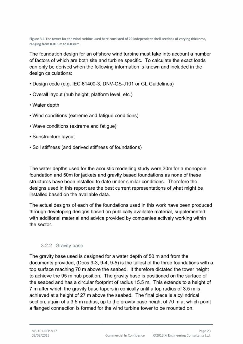
Figure 3-1 The tower for the wind turbine used here consisted of 29 independent shell sections of varying thickness,
ranging from 0.015 m to 0.038 m.
The foundation design for an offshore wind turbine must take into account a number of factors of which are both site and turbine specific. To calculate the exact loads can only be derived when the following information is known and included in the design calculations:
• Design code (e.g. IEC 61400-3, DNV-OS-J101 or GL Guidelines)
• Overall layout (hub height, platform level, etc.)
• Water depth
• Wind conditions (extreme and fatigue conditions)
• Wave conditions (extreme and fatigue)
• Substructure layout
• Soil stiffness (and derived stiffness of foundations)
The water depths used for the acoustic modelling study were 30m for a monopole foundation and 50m for jackets and gravity based foundations as none of these structures have been installed to date under similar conditions. Therefore the designs used in this report are the best current representations of what might be installed based on the available data.
The actual designs of each of the foundations used in this work have been produced through developing designs based on publically available material, supplemented with additional material and advice provided by companies actively working within the sector.
3.2.2 Gravity base
The gravity base used is designed for a water depth of 50 m and from the documents provided, (Docs 9-3, 9-4, 9-5) is the tallest of the three foundations with a top surface reaching 70 m above the seabed. It therefore dictated the tower height to achieve the 95 m hub position. The gravity base is positioned on the surface of the seabed and has a circular footprint of radius 15.5 m. This extends to a height of 7 m after which the gravity base tapers in conically until a top radius of 3.5 m is achieved at a height of 27 m above the seabed. The final piece is a cylindrical section, again of a 3.5 m radius, up to the gravity base height of 70 m at which point a flanged connection is formed for the wind turbine tower to be mounted on.

MS-101-REP-V17 Page 24 09/08/2013 Commercial In Confidence ©2013 Xi Engineering Consultants Ltd.
The base cylinder and conical section is modelled as a solid with an internal cavity, calculated to hold the required ballast mass, (Figure 3-2). The upper cylindrical section is modelled as shells, with thickness 0.12 m for the cylinder walls, (Doc 9-3) and a top flange thickness of 0.3 m.
Figure 3-2 Geometry of gravity base highlighting the cavity within the lower conical section which is filled with a ballast
mass. The vertical heights indicated have z = 0 m set at the surface of the seabed.

MS-101-REP-V17 Page 25 09/08/2013 Commercial In Confidence ©2013 Xi Engineering Consultants Ltd.
3.2.3 Jacket foundation
As with the gravity base the jacket foundation was required to be modelled in 50m of water. The overall structure of the jacket is the most complex of the three foundation types and can be seen in Figure 3-3.
Figure 3-3 Geometry of the jacket used for the near-field modelling. The primary supports of the angled sides are of
radius 0.6 m while the x-brace supports are smaller at a radius of 0.3 m. The vertical heights indicated have z = 0 m set
at the surface of the seabed.
The jacket geometry was created from Docs 9-5, 9-6, 9-7, 9-8 and consists of four angled sides with primary supports of radius 0.6 m. Connecting x-braces are formed on each side using cylinders of radius 0.3 m. The entire jacket structure is modelled using shell elements with variable thickness capabilities, here using an initial thickness of 0.06 m. The primary supports penetrate to a depth of 9.6 m with the top of the jacket reaching a height of 65 m above the seabed. A cylindrical transition piece is included of height 5 m forming the surface on which the wind turbine tower is to be mounted. The dimensions are consistent with the top section of the gravity base and it has been designed so that a hub height of 95 m is achieved such that the performance of the jacket foundation can be compared to that of the gravity base.

MS-101-REP-V17 Page 26 09/08/2013 Commercial In Confidence ©2013 Xi Engineering Consultants Ltd.
3.2.4 Monopile
Monopiles are typically used in shallower water and so here it is modelled in a water depth of 30 m. The monopile is formed from two cylinders connected by a flange at the surface of the sediment layer. The penetration depth of the lower section is 50 m into the seabed and the top surface of the monopile is 40 m above the sediment. Using the generic 75 m wind turbine tower and nacelle with a water depth of 30 m requires a 10 m transition piece to be included in order to compare a 95 m hub height for all three foundations, Figure 3-4. The monopile geometry is modelled using shell elements as per Docs 9-2, 9-9, 9-10 with a thickness of 0.06 m producing the first bending mode at 0.18 Hz which is in agreement with Doc 9-9. The transition piece surface is again consistent with that used for the gravity base and the jacket foundation.
Figure 3-4 Geometry of the modelled monopile penetrating a depth of 50 m into the seabed and including a transition
piece so that a consistent hub height of 95 m is achieved using the generic wind turbine. The vertical heights indicated
have z = 0 m set at the surface of the seabed.
3.2.5 Water acoustic domain
To fully characterise the structural-acoustic interaction between the foundation and the water a radially dependent acoustic domain is formed. The geometry is cylindrical. In order to capture the acoustic response of the source term the SPL is calculated a distance of 30 m from the centre of the foundation using a cylindrical surface probe. To avoid reflected boundary discrepancies the acoustic domain is

MS-101-REP-V17 Page 27 09/08/2013 Commercial In Confidence ©2013 Xi Engineering Consultants Ltd.
extended to a distance of 40 m allowing sufficient distance to minimise spurious results (Figure 3-5).
Figure 3-5 A cylindrical geometry is used for the acoustic domain. It extends 40 m from the centre of the foundation. A
surface probe is used to calculate the radially and depth dependent acoustic emission and is positioned 30 m from the
foundation centre.
3.2.6 Seabed domain
The seabed is modelled using solid elements and is comprised of a two part geometry. Again a cylindrical geometry is used extending to the external boundary of the acoustic domain. The two part separation forms an upper sediment layer of depth 7 m and a lower bedrock of depth 43 m so that the full extent of the deepest pile can be analysed, Figure 3-4.
3.3 Material properties
Structural steel was used for the wind turbine tower and nacelle as well as the jacket, monopile and cylindrical shell elements of the gravity base. The conical section of the gravity base was modelled as concrete while the cavity was filled with a ballast mass of 20 kilotonne of dense sands, (Docs 9-3, 9-5). The properties for the blades and nacelle were calculated to match the data provided in Docs 9-1, 9-2, 9-11. The acoustic domain was modelled as sea water with the sediment layer formed from dense sands. Table 3-1 presents the values used for these materials in the computational models.
The level of internal damping inherent to materials affects the dissipation of vibration energy and consequently the noise emitted. Internal damping of steel is less than

MS-101-REP-V17 Page 28 09/08/2013 Commercial In Confidence ©2013 Xi Engineering Consultants Ltd.
that of concrete and is accounted for in the structural-acoustic interaction models using an isotropic loss factor of 0.0025 for structural steel and 0.05 for concrete and dense sands.
MS-101-REP-V17 Page 29 09/08/2013 Commercial In Confidence ©2013 Xi Engineering Consultants Ltd.
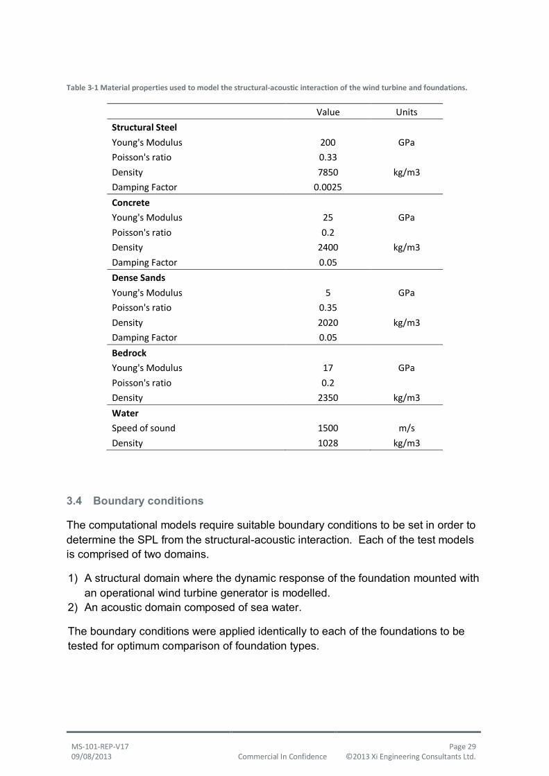
Table 3-1 Material properties used to model the structural-acoustic interaction of the wind turbine and foundations.
Value Units
Structural Steel
Young's Modulus 200 GPa
Poisson's ratio 0.33
Density 7850 kg/m3
Damping Factor 0.0025
Concrete
Young's Modulus 25 GPa
Poisson's ratio 0.2
Density 2400 kg/m3
Damping Factor 0.05
Dense Sands
Young's Modulus 5 GPa
Poisson's ratio 0.35
Density 2020 kg/m3
Damping Factor 0.05
Bedrock
Young's Modulus 17 GPa
Poisson's ratio 0.2
Density 2350 kg/m3
Water
Speed of sound 1500 m/s
Density 1028 kg/m3
3.4 Boundary conditions
The computational models require suitable boundary conditions to be set in order to determine the SPL from the structural-acoustic interaction. Each of the test models is comprised of two domains.
1) A structural domain where the dynamic response of the foundation mounted with an operational wind turbine generator is modelled.
2) An acoustic domain composed of sea water.
The boundary conditions were applied identically to each of the foundations to be tested for optimum comparison of foundation types.

MS-101-REP-V17 Page 30 09/08/2013 Commercial In Confidence ©2013 Xi Engineering Consultants Ltd.
3.4.1 Structural boundary conditions
The base of the bedrock is set as a fixed boundary while the cylindrical walls of both the bedrock and sediment layer have roller boundary conditions that restricts structural displacement normal to the cylindrical surface but otherwise it is free to move (Figure 3-6).
Figure 3-6 Structural boundary conditions applied to each of the foundation assemblies include a fixed base to the
bedrock, roller boundary to the seabed cylindrical surface and variable excitation forces to the gearbox and generator in
the nacelle.
The structural domain is excited by forces indicative of an operational wind turbine. These excitation forces originate from the drive train and are modelled using the gearbox and generator cylinders within the nacelle. The magnitude of the forces vary as a function of frequency such that they occur in discrete frequency bands related to both gear meshing and electro-magnetic (E-M) interaction between the spinning poles and stationary stators in the generator (i.e. it is a maximum at gear meshing / E-M interaction frequencies and close to zero elsewhere). The first 15 multiples of these excitation forces are applied as they can also result in triggering

MS-101-REP-V17 Page 31 09/08/2013 Commercial In Confidence ©2013 Xi Engineering Consultants Ltd.
structural resonances. This is achieved using peaks of force in the frequency domain F(f) that take the form of summed normal distributions according to:
where F(mesh/EM) is the force representing the gear meshing or EM interaction at each step-up stage (the model is calibrated by varying the value of this parameter), f is the frequency, σ is a shape term that defines the frequency range over which the gear meshing / EM interaction is effective and f(mesh/EM) is the gear meshing or EM interaction frequency. The magnitude of the excitation of the drive train is related to the torque acting on the rotor, which will be dependent on the wind speed.
The wind turbine used here is based on the specifications of the REPower 6MW with a 12.1 rpm at a rated wind speed of 14 ms-1, 1:97 transmission ratio and a three stage planetary gear system, Doc 9-11. The magnitudes used for these frequency dependent forces for the gear meshing and E-M interaction are presented in Figure 3-7 and Figure 3-8 respectively.
Figure 3-7 Excitation forces applied in the gearbox in the variable excitation models. The excitation forces represent
those caused by teeth of the gears meshing together. The first fifteen multiples of each of the gear-meshing frequencies
are also modelled. The amplitude of the excitation frequencies were estimated using previous measurements on similar
wind turbines.
(Eq 3.1)

MS-101-REP-V17 Page 32 09/08/2013 Commercial In Confidence ©2013 Xi Engineering Consultants Ltd.
Figure 3-8 Excitation forces applied to the generator to model the effects of E-M fluctuations. The amplitude of the
excitation frequencies were estimated using previous measurements on similar wind turbines.
The excitation forces applied to the drive train were calculated from the wind turbine specifications and compared to measurements of similar sized turbines carried out by Xi Engineering Consultants Ltd. The frequency parameters for the variable excitation used are shown in Table 3-2. The forces arising from the rotational motion of the drive train are modelled using the surface boundaries of the gear box and generator. It is assumed that the forces in the gear box and generator are proportional to the torque in the drive train and changes linearly with power. Figure 3-9 presents the Power curve for a REPower 6MW wind turbine (Doc 9-11). This enables the power, and therefore the force, for 5 ms-1, 10 ms-1 and 15 ms-1 to be calculated. The excitation forces are assigned to the surface boundaries of the gear box and generator, using Cartesian coordinates as indicated in Figure 3-6, with the magnitudes given in Table 3-3.
Table 3-2 Frequency parameters for the variable excitation forces applied to the drive train, representative of the wind
turbine used. σ is a shape term that defines the frequency range over which the gear meshing / EM interaction is
effective.
6MW Wind Turbine
Generator
Frequency (Hz)
σ
(Hz)
Gear Stage 1 30 3
Gear Stage 2 125 2.5
Gear Stage 3 600 2
Generator Poles 78 2
Generator Stators 117 2
Pole - Stator Interaction 469 2

MS-101-REP-V17 Page 33 09/08/2013 Commercial In Confidence ©2013 Xi Engineering Consultants Ltd.
Figure 3-9 Power curve for a REPower 6MW wind turbine, (Doc 9-11). This enables the forces in the gear box and
generator to be approximated for different wind speeds.
Table 3-3 Values of forces used to apply the variable excitation to the drive train. They are modelled using Cartesian
coordinates assigned to the cylindrical surfaces of the gearbox and generator components in the nacelle.
Wind Speed
v = 5 ms-1 v = 10 ms-1 v = 15 ms-1
Fmesh/EM
(Pa)
Fmesh/EM
(Pa)
Fmesh/EM
(Pa)
Gear Meshing (x) 10 92 170
Gear Meshing (y) 33 572 1056
Gear Meshing (z) 10.5 97.5 180
Generator E-M (x) 9.5 89 162
Generator E-M (y) 9 84 155
Generator E-M (z) 7 65 120
3.4.2 Acoustic boundary conditions
The upper and lower surfaces of the acoustic domain (sea surface and seabed) are assumed to be perfect reflectors of noise and so will result in an overestimate, (Section 2.2). Cylindrical wave radiation boundary conditions are applied to the vertical walls of the acoustic domain allowing pressure waves to propagate out of the model space. The boundary condition uses a simplification where the source of the

MS-101-REP-V17 Page 34 09/08/2013 Commercial In Confidence ©2013 Xi Engineering Consultants Ltd.
cylindrical wave is taken to be co-linear with the vertical axis at the foundation centre, Figure 3-10.
Figure 3-10 Acoustic boundary conditions used for the near-field foundation modelling. The sea surface and seabed are
modelled as perfect reflectors. Cylindrical wave radiation is applied to the remaining acoustic domain boundaries to
allow the pressure waves to continue propagating beyond the domain.
3.4.3 Structural-acoustic interaction
The structural and acoustic domains are coupled at their interface and modelled concurrently in the frequency domain. The surface acceleration of the foundation structure is monitored where in contact with the water and used to apply pressure to the acoustic domain, Figure 3-11. In this way the structural-borne vibration propagates into the water and radiates away as noise.

MS-101-REP-V17 Page 35 09/08/2013 Commercial In Confidence ©2013 Xi Engineering Consultants Ltd.
Figure 3-11 Coupling of the structural-acoustic interaction. Surface acceleration monitored at the boundary between
the foundation and the sea water is used to apply pressure to the acoustic domain enabling the SPL to be calculated.
3.5 Mesh parameters
A free tetrahedral mesh was created. In order to calculate the SPL for each of the foundations the mesh needed to be optimised. By doing so enhances computational efficiency without sacrificing numerical accuracy. Problematic areas in the models geometries were identified at interconnecting flanges and brace elements, Figure 3-12.
To ensure the surface accelerations at the structural-acoustic interaction were captured and transmitted to the acoustic domain accurately, a maximum mesh element size of 1.5 m was set where the foundation was submerged in the sea, Figure 3-13. The subsequent pressure transferred to the acoustic domain could be calculated, again limiting the maximum mesh element size for numerical accuracy, here with a value of 7.5 m, Figure 3-14.

MS-101-REP-V17 Page 36 09/08/2013 Commercial In Confidence ©2013 Xi Engineering Consultants Ltd.
Figure 3-12 Mesh optimisation of jacket foundation brace. Problematic edges were assigned distributions of appropriate
size for improved accuracy.
Figure 3-13 A maximum of 1.5 m mesh element size was applied to the foundation boundary of the structural - acoustic
interaction to enable accurate calculation of the surface acceleration and resultant pressure waves propagating into the
acoustic domain.
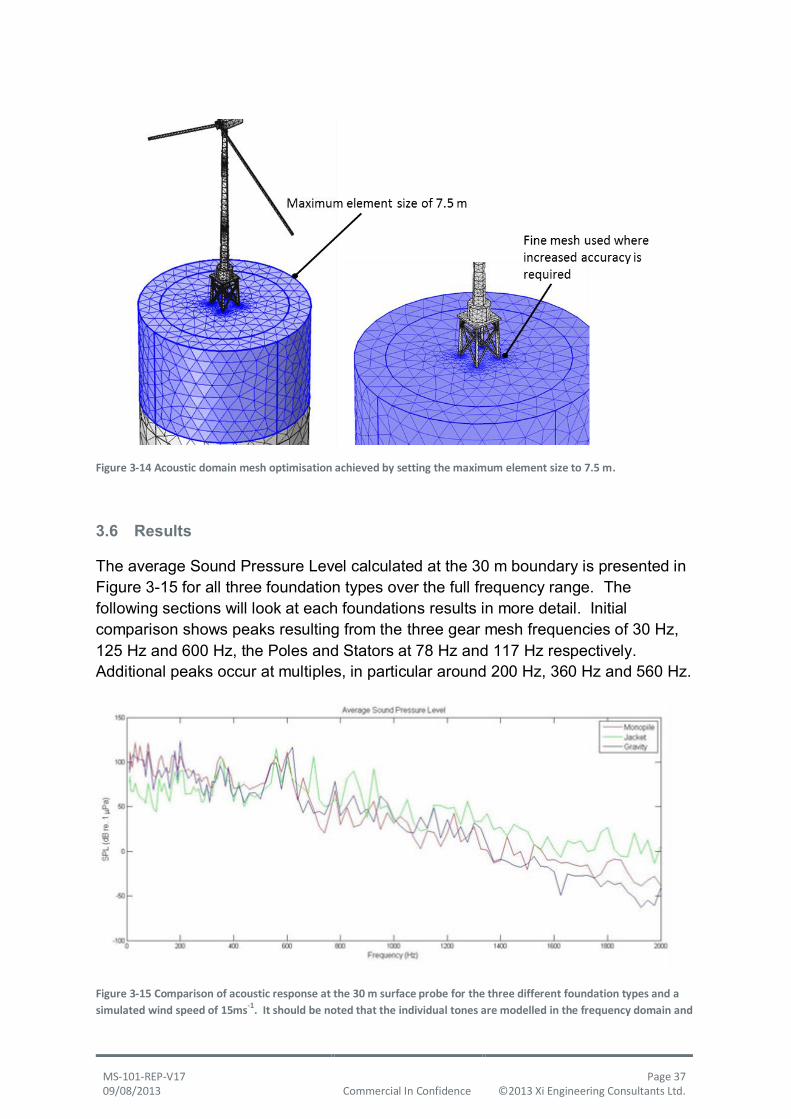
MS-101-REP-V17 Page 37 09/08/2013 Commercial In Confidence ©2013 Xi Engineering Consultants Ltd.
Figure 3-14 Acoustic domain mesh optimisation achieved by setting the maximum element size to 7.5 m.
3.6 Results
The average Sound Pressure Level calculated at the 30 m boundary is presented in Figure 3-15 for all three foundation types over the full frequency range. The following sections will look at each foundations results in more detail. Initial comparison shows peaks resulting from the three gear mesh frequencies of 30 Hz, 125 Hz and 600 Hz, the Poles and Stators at 78 Hz and 117 Hz respectively. Additional peaks occur at multiples, in particular around 200 Hz, 360 Hz and 560 Hz.
Figure 3-15 Comparison of acoustic response at the 30 m surface probe for the three different foundation types and a
simulated wind speed of 15ms-1
. It should be noted that the individual tones are modelled in the frequency domain and
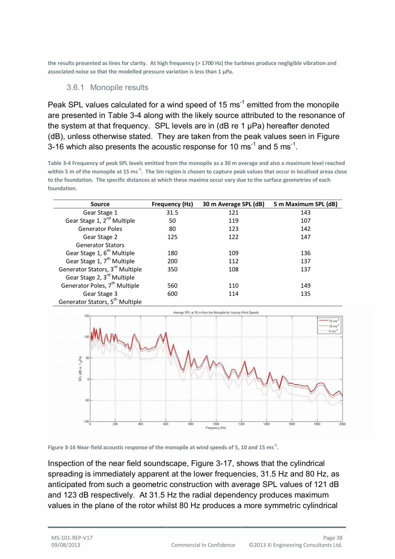
MS-101-REP-V17 Page 38 09/08/2013 Commercial In Confidence ©2013 Xi Engineering Consultants Ltd.
the results presented as lines for clarity. At high frequency (> 1700 Hz) the turbines produce negligible vibration and
associated noise so that the modelled pressure variation is less than 1 μPa.
3.6.1 Monopile results
Peak SPL values calculated for a wind speed of 15 ms-1 emitted from the monopile are presented in Table 3-4 along with the likely source attributed to the resonance of the system at that frequency. SPL levels are in (dB re 1 µPa) hereafter denoted (dB), unless otherwise stated. They are taken from the peak values seen in Figure 3-16 which also presents the acoustic response for 10 ms-1 and 5 ms-1.
Table 3-4 Frequency of peak SPL levels emitted from the monopile as a 30 m average and also a maximum level reached
within 5 m of the monopile at 15 ms-1. The 5m region is chosen to capture peak values that occur in localised areas close
to the foundation. The specific distances at which these maxima occur vary due to the surface geometries of each
foundation.
Source Frequency (Hz) 30 m Average SPL (dB) 5 m Maximum SPL (dB)
Gear Stage 1 31.5 121 143 Gear Stage 1, 2nd Multiple 50 119 107
Generator Poles 80 123 142 Gear Stage 2
Generator Stators 125 122 147
Gear Stage 1, 6th Multiple 180 109 136 Gear Stage 1, 7th Multiple 200 112 137
Generator Stators, 3rd Multiple Gear Stage 2, 3rd Multiple
350 108 137
Generator Poles, 7th Multiple 560 110 149 Gear Stage 3
Generator Stators, 5th Multiple 600 114 135
Figure 3-16 Near-field acoustic response of the monopile at wind speeds of 5, 10 and 15 ms-1.
Inspection of the near field soundscape, Figure 3-17, shows that the cylindrical spreading is immediately apparent at the lower frequencies, 31.5 Hz and 80 Hz, as anticipated from such a geometric construction with average SPL values of 121 dB and 123 dB respectively. At 31.5 Hz the radial dependency produces maximum values in the plane of the rotor whilst 80 Hz produces a more symmetric cylindrical

MS-101-REP-V17 Page 39 09/08/2013 Commercial In Confidence ©2013 Xi Engineering Consultants Ltd.
spreading. Maximum values within 5 m of the monopile are 143 dB for 31.5 Hz and 142 dB for 80 Hz.
The cylindrical spreading at the higher frequency of 180 Hz exhibits more interference when spreading from the monopile, typical from the additional maxima / minima caused by a pulsing cylindrical source reflected from the water surface and seabed, with a 30 m average SPL of 109 dB and a 5 m maximum of 136 dB. The continued scatter resulting from higher frequencies produces comparable SPL levels at 600 Hz of 114 dB for the 30 m average and 135 dB for the 5 m maximum.
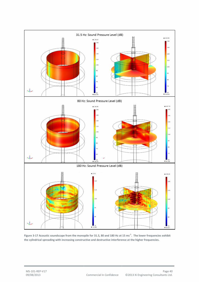
MS-101-REP-V17 Page 40 09/08/2013 Commercial In Confidence ©2013 Xi Engineering Consultants Ltd.
Figure 3-17 Acoustic soundscape from the monopile for 31.5, 80 and 180 Hz at 15 ms-1. The lower frequencies exhibit
the cylindrical spreading with increasing constructive and destructive interference at the higher frequencies.

MS-101-REP-V17 Page 41 09/08/2013 Commercial In Confidence ©2013 Xi Engineering Consultants Ltd.
3.6.2 Gravity results
Peak SPL values calculated for a wind speed of 15 ms-1 emitted from the gravity base are presented in Table 3-5 along with the likely source attributed to the resonance of the system at that frequency. They are taken from the peak values seen in Figure 3-18 which also presents the acoustic response for 10ms-1 and 5ms-1.
Inspection of the near field soundscape, Figure 3-19, again shows cylindrical spreading is apparent at the lower frequencies, 31.5 Hz and 80 Hz with average SPL values of 105 dB and 111 dB respectively. At 31.5 Hz the radial dependency again produces maximum values in the plane of the rotor with additional constructive/destructive interference from the conical section of the gravity base whilst 80 Hz produces peak values in the plane of the wind direction (x-z plane). Maximum values within 5 m of the gravity base are 127 dB for 31.5 Hz and 134 dB for 80 Hz.
Table 3-5 Frequency of peak SPL levels emitted from the gravity base as a 30 m average and also a maximum level
reached within 5 m of the gravity base at 15 ms-1.
Source Frequency (Hz) 30 m Average SPL (dB) 5 m Maximum SPL (dB) Gear Stage 1 31.5 105 127
Generator Poles 80 111 134 Gear Stage 2
Generator Stators 125 94 125
Gear Stage 1, 5th Multiple Generator Poles, 2nd Multiple
150 96 106
Gear Stage 1, 6th Multiple 180 116 133 Gear Stage 1, 7th Multiple 200 128 152
Generator Stators, 3rd Multiple Gear Stage 2, 3rd Multiple
350 97 126
Generator Poles, 7th Multiple 560 101 112 Gear Stage 3
Gear Stage 2, 5th
Multiple 620 116 143
Figure 3-18 Near-field acoustic response of the gravity base at wind speeds of 5, 10 and 15ms-1.

MS-101-REP-V17 Page 42 09/08/2013 Commercial In Confidence ©2013 Xi Engineering Consultants Ltd.
Figure 3-19 Acoustic soundscape from the gravity base for 31.5, 80 and 125 Hz at 15 ms-1. The lower frequencies exhibit
the cylindrical spreading. At 125 Hz a similar response to the monopile can be seen emitting from the upper cylindrical
section of the gravity base.

MS-101-REP-V17 Page 43 09/08/2013 Commercial In Confidence ©2013 Xi Engineering Consultants Ltd.
At the higher frequency of 125 Hz the acoustic soundscape exhibits more interference when spreading from the gravity base. The upper cylindrical section of the gravity base has a similar acoustic response to that of the monopile, here with lower levels of 94 dB for the 30 m average SPL and a 5 m maximum of 125 dB. The SPL again peaks near the Gear Stage 3 with a 30 m average of 116 dB at 620 Hz and 143 dB for the 5 m maximum.
3.6.3 Jacket results
Peak SPL values calculated for a wind speed of 15ms-1 emitted from the jacket foundation are presented in Table 3-6 along with the likely source attributed to the resonance of the system at that frequency. They are taken from the peak values seen in Figure 3-20 which also presents the acoustic response for 10ms-1 and 5ms-1.
Table 3-6 Frequency of peak SPL levels emitted from the jacket foundation as a 30 m average and also a maximum level
reached within 5 m of the jacket at 15 ms-1.
Source Frequency (Hz) 30 m Average SPL (dB) 5 m Maximum SPL (dB)
Gear Stage 1 31.5 81 115 Generator Poles 80 76 116
Gear Stage 2 Generator Stators
120 82 127
Gear Stage 1, 5th Multiple Generator Poles, 2nd Multiple
140 76 113
Gear Stage 1, 6th Multiple 180 93 125 Gear Stage 1, 7
th Multiple 200 94 123
Generator Stators, 3rd Multiple Gear Stage 2, 3rd Multiple
350 101 131
Generator Poles, 7th Multiple 560 119 158 Gear Stage 3
Generator Stators, 5th
Multiple 600 101 136
Generator Poles, 9th
Multiple Generator Stators, 6
th Multiple
700 106 177
Gear Stage 2, 7th
Multiple Generator Stators, 7
th Multiple
850 90 179
Generator Stators, 8th
Multiple Generator Poles and Stators,
2nd Multiple
925 92 191

MS-101-REP-V17 Page 44 09/08/2013 Commercial In Confidence ©2013 Xi Engineering Consultants Ltd.
Figure 3-20 Near-field acoustic response of the jacket foundation at wind speeds of 5, 10 and 15ms-1.
The lower frequencies produce acoustic responses consistent with cylindrical spreading, Figure 3-21. Average SPL Values of 81 dB and 76 dB are reached at the 30 m surface probe for 31.5 Hz and 80 Hz respectively with maximum levels of 115 dB and 116 dB within 5 m of the jacket for these frequencies. The highest SPL calculated was for 560 Hz, with a 30 m average SPL of 119 dB and 5 m maximum of 158 dB. Furthermore higher frequencies produce significant SPL with 30 m averages of 106 dB at 700 Hz, 90 dB at 850 Hz and 92 dB at 925 Hz and 5 m maximum SPL values of 177 dB, 179 dB and 191 dB respectively.

MS-101-REP-V17 Page 45 09/08/2013 Commercial In Confidence ©2013 Xi Engineering Consultants Ltd.
Figure 3-21 Acoustic soundscape from the jacket foundation for 31.5, 80 and 560 Hz at 15 ms-1. The lower frequencies
exhibit the cylindrical spreading. The more complex lattice structure produces a noisier soundscape at the higher
frequencies with greater SPL values achieved.

MS-101-REP-V17 Page 46 09/08/2013 Commercial In Confidence ©2013 Xi Engineering Consultants Ltd.
3.6.4 Comparison of peak SPL values
An initial comparison of the acoustic response for each of the three foundation types was presented in Figure 3-15. Inspection of the maximum SPL peaks and respective frequencies are summarised below in Table 3-7.
At frequencies lower than 180 Hz the monopile produces the largest amount of noise. Of the three foundation types the monopile continues to produce larger SPL values up to 500Hz. While the gravity base produces the largest average SPL values at the 30 m surface probe for 180 Hz and 200 Hz the peaks are sharper and the surrounding frequencies are of lower SPL values, Figure 3-15. Also apparent from Figure 3-15 is that around 600 Hz all three foundation types become comparable in average 30 m SPL with the trend of the jacket foundation rising to become the noisiest at frequencies greater than 700 Hz.
Generally the maximum level achieved within 5 m of the foundation coincides with the largest 30 m average level. The clear discrepancy from Table 3-7 being the jacket foundation at 120 Hz. Figure 3-22 presents the acoustic soundscape for the jacket at 120 Hz showing localised bursts of high sound intensity around the lattice but insufficient to propagate far from the foundation itself due to the small sizes of surface area producing these tones.
Table 3-7 Summary of near-field SPL values produced from each of the three foundation types at 15 ms-1. The
frequency at which the 30 m average SPL value peaks is given in the first column. Where foundation types have similar
peaks the corresponding frequency is denoted (M) Monopile, (G) Gravity Base, (J) Jacket. The monopile typically
produces the largest noise levels at the lower frequencies. The jacket produces the largest noise levels at the higher
frequencies.
Monopile Gravity Base Jacket
Frequency (Hz) 30 m Average SPL (dB)
5 m Max SPL (dB)
30 m Average SPL (dB)
5 m Max SPL (dB)
30 m Average SPL (dB)
5 m Max SPL (dB)
31.5 121 143 105 127 81 115
80 123 142 111 134 76 116
120 100 123 92 117 82 127
125 122 147 94 125 78 131
180 109 136 116 133 93 125
200 112 137 128 152 94 123
350 108 137 97 126 101 131
470(G,J) / 480(M)
74 99 71 112 67 99
560 110 149 101 139 119 158
600(M,J) / 620(G)
114 135 116 143 101 136
660(M) / 680(G) / 700(J)
85 158 57 129 106 177
825(M) / 850(G,J)
53 152 62 159 90 179
925(M,J) / 950G)
61 171 62 166 92 191
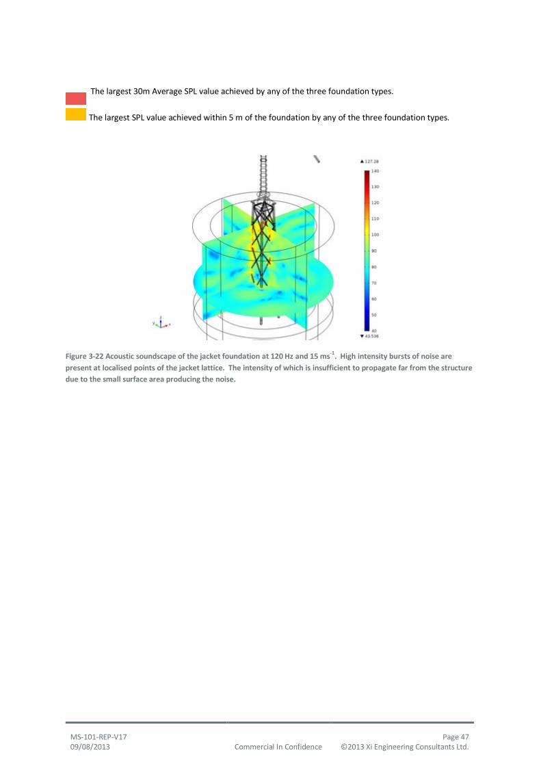
MS-101-REP-V17 Page 47 09/08/2013 Commercial In Confidence ©2013 Xi Engineering Consultants Ltd.
The largest 30m Average SPL value achieved by any of the three foundation types.
The largest SPL value achieved within 5 m of the foundation by any of the three foundation types.
Figure 3-22 Acoustic soundscape of the jacket foundation at 120 Hz and 15 ms-1. High intensity bursts of noise are
present at localised points of the jacket lattice. The intensity of which is insufficient to propagate far from the structure
due to the small surface area producing the noise.

MS-101-REP-V17 Page 48 09/08/2013 Commercial In Confidence ©2013 Xi Engineering Consultants Ltd.
4 FAR-FIELD ACOUSTIC MODEL
4.1 Beam trace model
The sound field in the marine environment up to 20 km from wind farms consisting of 16 turbines that are founded on jackets, gravity bases and monopiles were modelled. The sound field for each foundation type was modelled using a Gaussian beam trace model (AcTUP, produced by Centre for Marine Science and Technology at Curtin University, Australia). Coherent transmission loss was modelled through two dimensional vertical sections radiating from the wind turbine foundation. To simplify the model it was assumed that there was no surface roughness and that the speed of sound profile was linear.
The acoustic outputs of the near-field models were used as ‘source terms’ in the far-field model. The source terms were taken as the SPL 30m from the central axis of each near-field model calculated at 5m depth and 5° radial intervals. The sound field of each vertical radial section was calculated by subtracting the transmission loss field from the source term related to the radial section: in this way any directionality of the near-field models is transposed into the far-field analysis. The coordinate system used in the near-field model was followed in the far field model; thus the positive x-direction is taken as the wind direction and it is assumed that all wind turbines in each wind farm was oriented in the same direction.
Each of the resulting 2-dimensional vertical sound fields were compiled using the computer package Matlab, to produce a 3-dimension cylindrical sound field with a diameter of 40 km and a depth of 30 m wind farms founded on monopiles and 50 m for farms founded on jackets and gravity bases. The sound field was modelled in one-third octave frequency bands between 10 and 2000 Hz.
4.2 Geometry and material properties
The two-dimension vertical transmission loss field for monopiles was modelled as 30 m of water, overlaying a 7 m elastic domain that represents sediment which overlies an elastic half space representing the bedrock. The transmission loss fields for the jacket and gravity base were modelled with a 50m water depth overlying 7m of sediment and a bedrock half space. The material properties of the water, sediment and bedrock domains are shown in Table 4-1.
Two wind farm layouts were modelled based on information provided by Marine Scotland:
1. Diamond layout 2. Square layout

MS-101-REP-V17 Page 49 09/08/2013 Commercial In Confidence ©2013 Xi Engineering Consultants Ltd.
These layouts are shown in Figure 4-1. To make comparison between wind farm layouts possible the same spacings were used in the down-wind direction (840 m) and across wind (600 m) for both layouts.
Table 4-1 Material properties used in far-field models
Speed of Sound Density
m/s kg/m3
Water 1500 1028
Sediment 1658 2020
Bedrock 2004 2350
A – Diamond layout
B – Square layout
Figure 4-1 – wind farm layouts used to model the far field noise output. A) Diamond wind farm layout. B) Square wind
farm layout
4.3 Results
The modelled sound fields tend to be cylindrical about wind farms, with little variation in sound pressure level with respect to depth. Figure 4-2 shows a vertical cross-section through the sound field in the 16 Hz one-third octave band modelled from a diamond shaped layout; the sound field distribution in this one-third octave band is representative of the other one-third octave bands modelled. Figure 4-2 shows that the SPL is strongly dependent on the horizontal distance from the centre of the wind farm, with only a slight increase in SPL with depth (i.e. almost a perfect cylindrical pattern).
The diamond and square layouts of wind farms were compared and little difference was found in the modelled sound fields (Figure 4-3). The modelled spectra shown in Figure 4-3 are for wind turbines founded on gravity bases; little difference between diamond and square layouts were found for either jacket or monopile foundations.
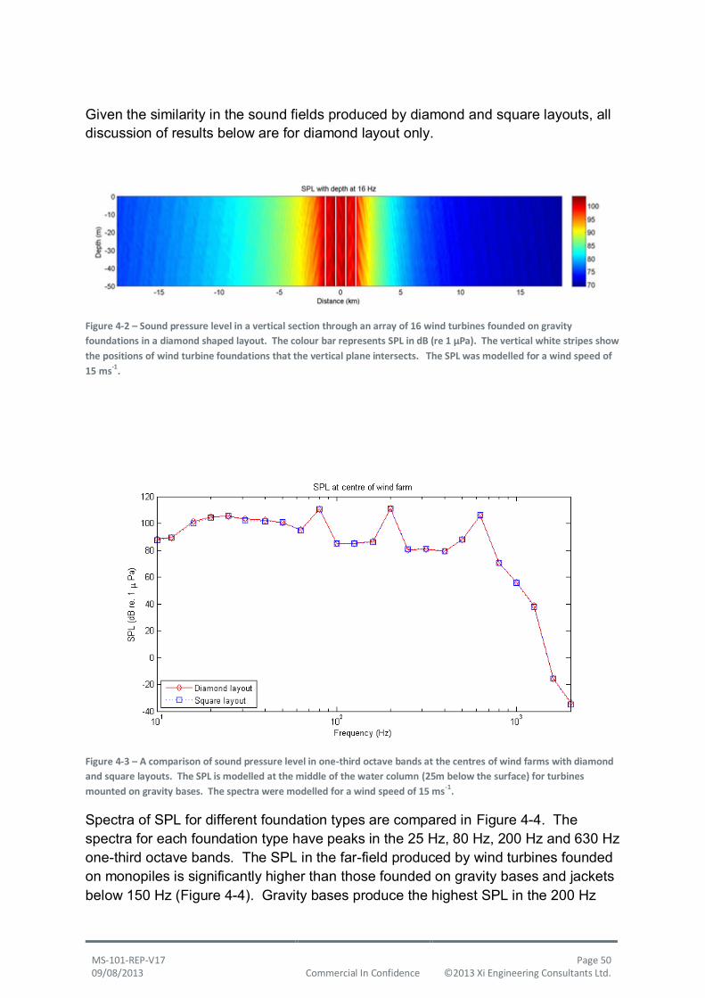
MS-101-REP-V17 Page 50 09/08/2013 Commercial In Confidence ©2013 Xi Engineering Consultants Ltd.
Given the similarity in the sound fields produced by diamond and square layouts, all discussion of results below are for diamond layout only.
Figure 4-2 – Sound pressure level in a vertical section through an array of 16 wind turbines founded on gravity
foundations in a diamond shaped layout. The colour bar represents SPL in dB (re 1 μPa). The vertical white stripes show
the positions of wind turbine foundations that the vertical plane intersects. The SPL was modelled for a wind speed of
15 ms-1.
Figure 4-3 – A comparison of sound pressure level in one-third octave bands at the centres of wind farms with diamond
and square layouts. The SPL is modelled at the middle of the water column (25m below the surface) for turbines
mounted on gravity bases. The spectra were modelled for a wind speed of 15 ms-1.
Spectra of SPL for different foundation types are compared in Figure 4-4. The spectra for each foundation type have peaks in the 25 Hz, 80 Hz, 200 Hz and 630 Hz one-third octave bands. The SPL in the far-field produced by wind turbines founded on monopiles is significantly higher than those founded on gravity bases and jackets below 150 Hz (Figure 4-4). Gravity bases produce the highest SPL in the 200 Hz

MS-101-REP-V17 Page 51 09/08/2013 Commercial In Confidence ©2013 Xi Engineering Consultants Ltd.
and 630 Hz one-third octave bands. Jackets produce the high SPL at frequencies above 800 Hz (Figure 4-4).
The sound fields produced by the wind farms can be strongly direction. Figure 4-5 shows an example of the directionality of the sound-field in the 20 Hz one-third octave band; the sound fields of all one-third octave bands are shown in Appendix B. The directionality of the sound field varies with frequency and foundation type. The highest SPL tend to be in the plane of the rotor (i.e. cross-wind) (see Appendix B), though in some cases the highest SPL is modelled up- and down-wind of the wind farm (e.g. gravity base at 80 Hz, see Figure 4-6).
The sound produced by wind farms can be masked by the background noise. Masking occurs when the SPL produced by wind turbines is less than the background level. The spectra in Figure 4-4 are shown with the background noise level for sea state 6 (Figure 2-2). The sound produced by the wind farm mounted on jackets is masked for all frequencies modelled except for the 400 Hz to 800 Hz one-third octave bands. Contours showing where the SPL produced by the wind farm is equal to the background noise level for each one-third octave band are shown in Appendix B, Figure 4-5 and Figure 4-6: the sound produced by the wind farms is effectively masked on the outside of these contours and therefore cannot be heard by marine species. The maximum range at which the wind farm is audible above the background noise is shown in Figure 4-7. At 5 ms-1 the turbines mounted on monopiles and gravity bases are audible at 25, 80 and 200 Hz at least 18 km away, whereas the jacket based turbine are only audible at 630 Hz (Figure 4-7). At 10 and 15 ms-1 the monopile and gravity bases are audible at least 18 km away at most frequencies below 800 Hz, while the jacket is audible at 250 Hz 10 km away and 630 Hz at least 18 km away (Figure 4-7).

MS-101-REP-V17 Page 52 09/08/2013 Commercial In Confidence ©2013 Xi Engineering Consultants Ltd.
Figure 4-4 – Comparison of SPL in one-third octave band for wind farms founded on gravity bases, jackets and
monopiles. The spectra were modelled for a wind speed of 15 ms-1. Spectra approximately 200 m down- and cross-wind
from the closest wind turbine are shown as are spectra 10 km down- and cross-wind from the centre of the wind farm.
The background SPL is based on the Wenz curve for a sea state 6 and converted to third-octave level.

MS-101-REP-V17 Page 53 09/08/2013 Commercial In Confidence ©2013 Xi Engineering Consultants Ltd.
Figure 4-5 – Sound field at 20 Hz in a horizontal section taken at the mid-water depth surrounding wind farms mounted
on different foundation types. The black dots show the location of the wind turbines and the white contour is where
the sound field is equal to the background level for this one-third octave band; outside of this contour the noise of the
wind farm is masked by the background noise.
Wind Direction

MS-101-REP-V17 Page 54 09/08/2013 Commercial In Confidence ©2013 Xi Engineering Consultants Ltd.
Figure 4-6 - Sound field at 80 Hz in a horizontal section taken at the mid-water depth surrounding wind farms mounted
on different foundation types. The gravity base has the highest SPL up- and down-wind of the wind farm, whereas the
monopile has the highest SPL in the cross-wind directions.
Wind Direction

MS-101-REP-V17 Page 55 09/08/2013 Commercial In Confidence ©2013 Xi Engineering Consultants Ltd.
Figure 4-7 – Maximum range from the centre of a diamond shaped wind farm that wind turbines are audible above the
background noise as a function of frequency in Hz. Turbines mounted on gravity bases, jackets and monopiles are
compared at three different wind speeds. The Wenz curve used for 5 ms-1, 10 ms-1 and 15 ms-1 relate to sea states 2, 4
and 6 respectively converted to one-third octave levels. The dotted black line represents the boundary of the far-field
domain that was modelled; at points where the maximum range is above the dotted line represents maximum range lies
outside of the modelled domain.

MS-101-REP-V17 Page 56 09/08/2013 Commercial In Confidence ©2013 Xi Engineering Consultants Ltd.
5 EFFECT OF ACOUSTIC OUTPUT ON MARINE LIFE
5.1 Marine mammals
The potential effect that noise emitted from different foundation types may have on marine life can be examined by comparing the modelled near- and far-field sound pressure level to curves representing the hearing and behavioural response of marine species. Curves that characterise the hearing and behaviour of four marine mammals were examined: bottlenose dolphins, porpoise, minke whales and grey and harbour seals (together). These species represent marine mammals that are common in Scottish waters. Composite audiograms that represent the low frequency hearing thresholds of the marine mammal species are shown in Figure 5-1 (see section 2.5.1 for details of audiogram compilation).
Figure 5-1 – Audiograms of marine mammals; see section 2.5.1 for information on audiogram compilation.

MS-101-REP-V17 Page 57 09/08/2013 Commercial In Confidence ©2013 Xi Engineering Consultants Ltd.
Table 5-1 – Parameters representing the behavioural response and risk of injury to marine mammal species [SMRU
REFS]
Species Seals Harbour porpoise
Bottlenose dolphin
Minke Whale
Functional hearing group Pinniped in
water
High-frequency cetacean
Mid-frequency cetacean
Low-frequency cetacean
M-weighting
Estimated auditory band minimum
75 Hz 200 Hz 150 Hz 7 Hz
Estimated auditory band maximum
75 kHz 180 kHz 160 kHz 22 kHz
Sensation :
Added to one-third octave
bands
Lower 45 49 49 49
Upper 59
Behavioural response SPLs
(RMS)
10% response 135 90 120 120
50% response -- 120 140 140
90% response 144 140 160 160
5.1.1 Audibility zones
The sound field produced by each wind farm can be examined to determine where the SPL is greater than the hearing threshold of each species for any given frequency. The audiograms shown in Figure 5-1 were applied in this way to the modelled far-field sound field and the maximum range at which marine mammals could hear the wind farm determined as a function of frequency (Figure 5-2 to Figure 5-5). It is assumed that if the background noise exceeds the SPL produced by the wind farm that the noise from the farm is masked and cannot be detected by marine species. Thus, the maximum range at which species can hear the wind farm is less than or equal to the range shown in Figure 4-7.
Of the species of interest considered here, the minke whale has the most sensitive (i.e. best) hearing at low frequency (<2000 Hz) (Figure 5-1). The modelling outputs

MS-101-REP-V17 Page 58 09/08/2013 Commercial In Confidence ©2013 Xi Engineering Consultants Ltd.
predict that minke whales are able to detect the wind farm (with monopile or gravity foundations) at least 18 km away (Figure 5-3) at most frequencies below 800 Hz under all three wind conditions modelled. A minke whale could also detect a wind farm founded on jackets at 630 Hz at all three wind speeds (Figure 5-3) at large ranges. The seal species have less sensitive hearing than minke whales, particularly at very low frequencies (<100 Hz) (Figure 5-1), resulting in seals not being able to detect the wind farm below 100 Hz independent of wind speed or foundation type (Figure 5-2). However, seals can detect the wind farm up to at least 18 km in one third octave bands between 125 and 630 Hz at all wind speed conditions (Figure 5-2). Bottlenose dolphins and harbour porpoises are less sensitive to low frequency sound than either minke whales or the seals species. However both species can still detect the operating wind farm under different foundation and wind speed scenarios. Harbour porpoises can only detect the jacket foundation wind turbines in the 630 Hz band at wind speeds of 10 ms-1 and 15 ms-1 out to 4 km and 11 km respectively but can detect the gravity and monopile foundations out to at least 18 km (Figure 5-4). A bottlenose dolphin can detect a wind farm mounted on a gravity base 4 km away in wind speeds of 10 ms-1 and 15 km at 15 ms-1; though it can detect jackets and monopiles only at close ranges of ~1 km (Figure 5-5).

MS-101-REP-V17 Page 59 09/08/2013 Commercial In Confidence ©2013 Xi Engineering Consultants Ltd.
Figure 5-2 – Maximum range at which a harbour seal could hear a wind farm at different wind speeds. Gravity base,
jacket and monopile foundations are compared. It is assumed that if the SPL is below the background noise that a seal
could not hear the wind farm. The range is measured to the centre of the wind farm.

MS-101-REP-V17 Page 60 09/08/2013 Commercial In Confidence ©2013 Xi Engineering Consultants Ltd.
Figure 5-3 - Maximum range at which a minke whale could hear a wind farm at different wind speeds. Gravity base,
jacket and monopile foundations are compared. It is assumed that if the SPL is below the background noise that a
minke whale could not hear the wind farm. The range is measured to the centre of the wind farm.

MS-101-REP-V17 Page 61 09/08/2013 Commercial In Confidence ©2013 Xi Engineering Consultants Ltd.
Figure 5-4 - Maximum range at which a porpoise could hear a wind farm at different wind speeds. Gravity base, jacket
and monopile foundations are compared. It is assumed that if the SPL is below the background noise that a porpoise
could not hear the wind farm. The range is measured to the centre of the wind farm.
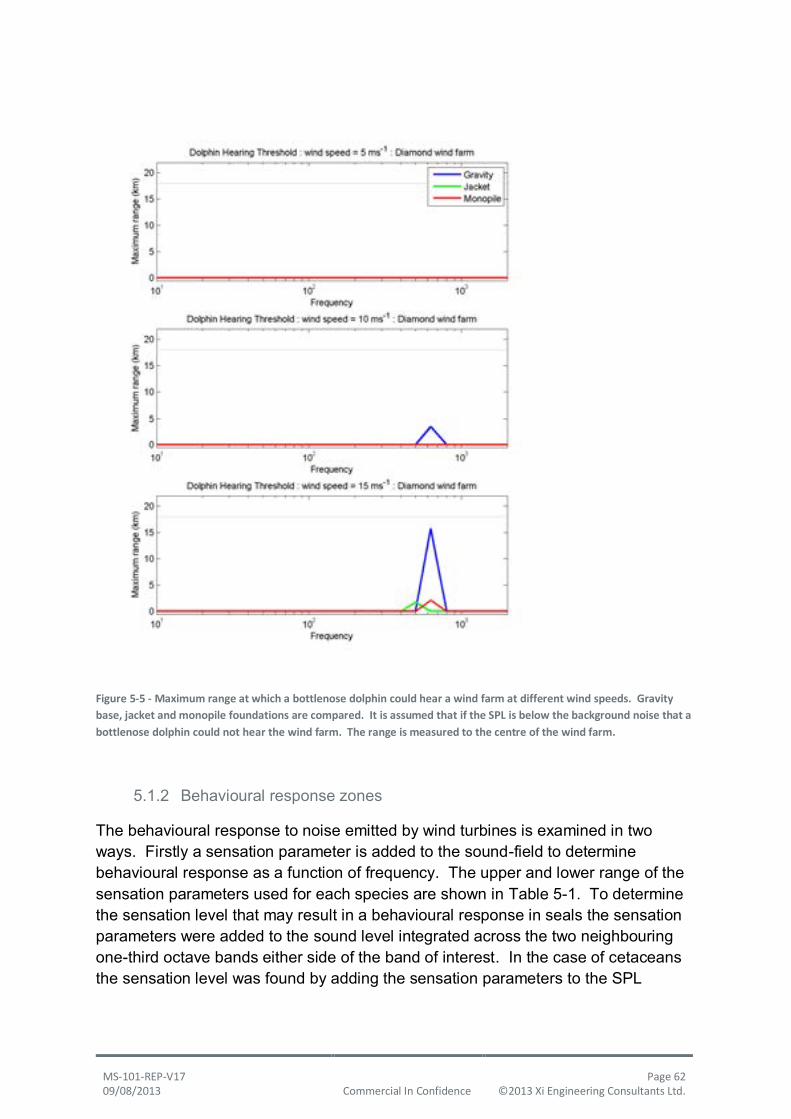
MS-101-REP-V17 Page 62 09/08/2013 Commercial In Confidence ©2013 Xi Engineering Consultants Ltd.
Figure 5-5 - Maximum range at which a bottlenose dolphin could hear a wind farm at different wind speeds. Gravity
base, jacket and monopile foundations are compared. It is assumed that if the SPL is below the background noise that a
bottlenose dolphin could not hear the wind farm. The range is measured to the centre of the wind farm.
5.1.2 Behavioural response zones
The behavioural response to noise emitted by wind turbines is examined in two ways. Firstly a sensation parameter is added to the sound-field to determine behavioural response as a function of frequency. The upper and lower range of the sensation parameters used for each species are shown in Table 5-1. To determine the sensation level that may result in a behavioural response in seals the sensation parameters were added to the sound level integrated across the two neighbouring one-third octave bands either side of the band of interest. In the case of cetaceans the sensation level was found by adding the sensation parameters to the SPL

MS-101-REP-V17 Page 63 09/08/2013 Commercial In Confidence ©2013 Xi Engineering Consultants Ltd.
integrated across the four neighbouring bands on the dominant side of the band of interest.
Potential behavioural response zones were calculated for each of the five marine mammal species of interest using three different metrics (section 2.4.1). This behavioural response zone considers masking by background noise, i.e. if the background noise exceeds the noise produce by operational wind turbines then the marine species are assumed not to change their behaviour. The results suggest a marked variation in response between the species (Table 5-2). Neither seal species nor bottlenose dolphins were predicted to exhibit a behavioural response to the sounds generated under any of the operational wind turbine scenarios. This means the predicted sound levels were lower than those required to elicit a behavioural response.
Harbour porpoises were only predicted to exhibit an aversive behavioural response using the M-weighting metric where 10% of animals encountering the noise field were expected to move away (Table 5-2). The ‘10% avoidance ranges’ varied depending on the foundation used and the wind speed. At low wind speeds (i.e. 5 ms-1) ranges were between 0 (jacket) and 1.7 km (monopile). At higher wind speeds (10 & 15 ms-1), avoidance ranges were predicted to be between 9.45 km (jacket foundation / 10 ms-1) and 18.84 km (monopile foundation / 10 & 15 ms-1). Avoidance ranges where 50% or 90% of porpoises were predicted to respond were not generated in any of the scenarios and therefore most harbour porpoises are not expected to respond to the operational noise.
Minke whales were determined to be more sensitive to the wind turbine noise than the other species of interest. For all metrics, the behavioural response ranges were largest for the monopile foundation, followed by the gravity base and lowest for the jacket foundation. As with the harbour porpoises, the minke whale behavioural response ranges increased as wind speed increased. The sensation level metric used indicated ranges of up to 18.84 km (Table 5-2, Figure 5-6 and Figure 5-7). However, the reverse-audiogram weighting and M-weighting approaches suggest that 10% of animals encountering the noise field were expected to move away at ranges between 3.7 km (RA-weighting) and 12.71 km (M-weighting from the source (both when wind speed is 15 ms-1).

MS-101-REP-V17 Page 64 09/08/2013 Commercial In Confidence ©2013 Xi Engineering Consultants Ltd.
Table 5-2 - Behavioural response zones for each species, foundation and wind speed scenario modelling here. The
sensation levels and weighted (M-weighting and reverse audiogram weighting) response ranges are shown (in km). For
the Reverse Audiogram and Southall m-weighting, the thresholds correspond to the SPLs at which 10%, 50% and 90% of
animals encountering it, are predicted to respond. The absolute threshold is shown for each species for reference.
Species Foundation Wind speed Lower Upper 10% 50% 90% 10% 50% 90%
Minke whale 49 -- 120 140 160 120 140 160
Gravity 5ms-1 0 -- 0 0 0 0 0 0
10ms-1 18.57 -- 0 0 0 1.58 0 0
15ms 18.84 -- 1.7 0 0 4.67 0 0
Jacket 5ms-1 0 -- 0 0 0 0 0 0
10ms-1 7.36 -- 0 0 0 0 0 0
15ms-1 18.18 -- 0 0 0 0 0 0
Monopile 5ms-1 2 -- 0 0 0 0 0 0
10ms-1 18.84 -- 1.7 0 0 4.81 0 0
15ms-1 18.84 -- 3.7 0 0 12.71 0 0
Seals 45 59 -- 135 144 -- 135 144
Gravity 5ms-1 0 0 0 0 0 0 0 0
10ms-1 0 0 0 0 0 0 0 0
15ms-1 0 0 0 0 0 0 0 0
Jacket 5ms-1 0 0 0 0 0 0 0 0
10ms-1 0 0 0 0 0 0 0 0
15ms-1 0 0 0 0 0 0 0 0
Monopile 5ms-1 0 0 0 0 0 0 0 0
10ms-1 0 0 0 0 0 0 0 0
15ms-1 0 0 0 0 0 0 0 0
Bottlenose dolphin 49 -- 120 140 160 120 140 160
Gravity 5ms-1 0 -- 0 0 0 0 0 0
10ms-1 0 -- 0 0 0 0 0 0
15ms-1 0 -- 0 0 0 0 0 0
Jacket 5ms-1 0 -- 0 0 0 0 0 0
10ms-1 0 -- 0 0 0 0 0 0
15ms-1 0 -- 0 0 0 0 0 0
Monopile 5ms-1 0 -- 0 0 0 0 0 0
10ms-1 0 -- 0 0 0 0 0 0
15ms-1 0 -- 0 0 0 0 0 0
Harbour porpoise 49 -- 90 120 140 90 120 140
Gravity 5ms-1 0 -- 0 0 0 1 0 0
10ms-1 0 -- 0 0 0 19 0 0
15ms-1 0 -- 0 0 0 19 0 0
Jacket 5ms-1 0 -- 0 0 0 0 0 0
10ms-1 0 -- 0 0 0 9.45 0 0
15ms-1 0 -- 0 0 0 18.58 0 0
Monopile 5ms-1 0 -- 0 0 0 1.7 0 0
10ms-1 0 -- 0 0 0 18.84 0 0
15ms-1 0 -- 0 0 0 18.84 0 0
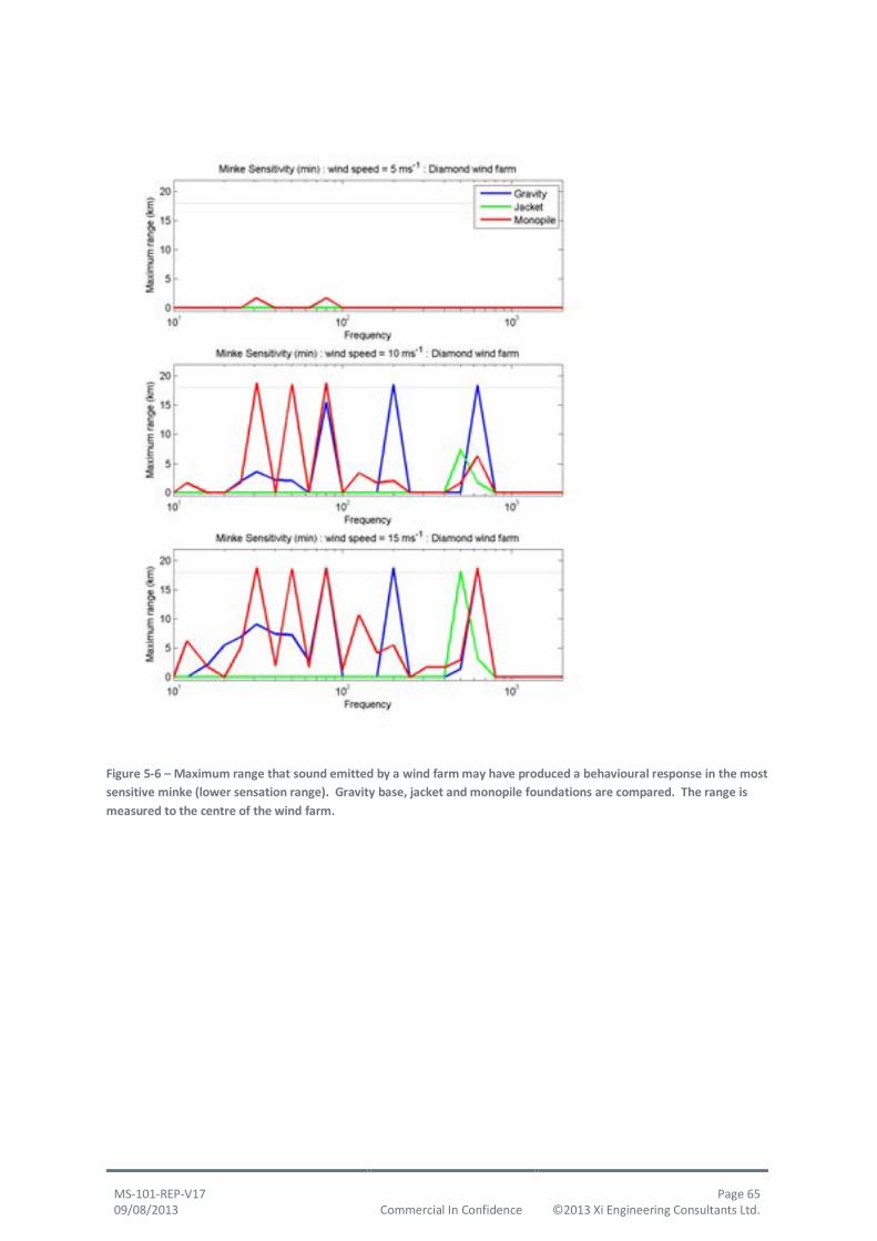
MS-101-REP-V17 Page 65 09/08/2013 Commercial In Confidence ©2013 Xi Engineering Consultants Ltd.
Figure 5-6 – Maximum range that sound emitted by a wind farm may have produced a behavioural response in the most
sensitive minke (lower sensation range). Gravity base, jacket and monopile foundations are compared. The range is
measured to the centre of the wind farm.

MS-101-REP-V17 Page 66 09/08/2013 Commercial In Confidence ©2013 Xi Engineering Consultants Ltd.
Figure 5-7 - Maximum range that sound emitted by a wind farm may have produced a behavioural response in the least
sensitive minke (upper sensation range). Gravity base, jacket and monopile foundations are compared. The range is
measured to the centre of the wind farm.
5.2 Fish
Audiograms of four species of fish were applied to the far-field sound field to determine the range at which they could detect the wind farm. The species examined were European eels, allis shad, sea trout and Atlantic salmon (Figure 5-8). Of the four species examined European eel is most sensitive to low frequency sound (<300 Hz) (Figure 5-8) resulting in eel being able to detect sound produced by the modelled wind farm at the greatest range at low frequency (Figure 5-9 to Figure 5-12). Eels can detect wind turbines founded on monopiles up to at least 18 km operating at all wind speeds modelled (Figure 5-9). Eels can detect turbines mounted on gravity bases operating in 10 ms-1 and 15 ms-1, but are unable to detect turbines mounted on jackets at all in the far-field (Figure 5-9). Salmon cannot detect far-field noise from any of the foundation types at 5 ms-1, but can detect those
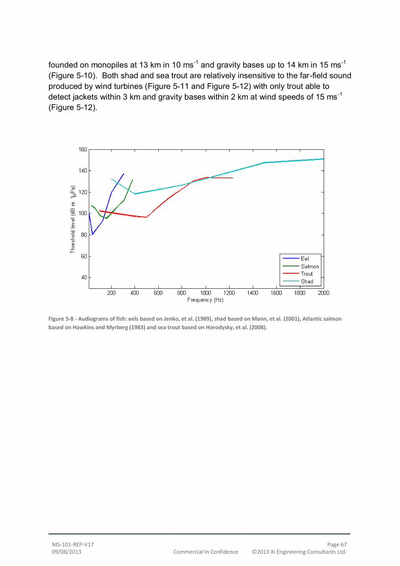
MS-101-REP-V17 Page 67 09/08/2013 Commercial In Confidence ©2013 Xi Engineering Consultants Ltd.
founded on monopiles at 13 km in 10 ms-1 and gravity bases up to 14 km in 15 ms-1 (Figure 5-10). Both shad and sea trout are relatively insensitive to the far-field sound produced by wind turbines (Figure 5-11 and Figure 5-12) with only trout able to detect jackets within 3 km and gravity bases within 2 km at wind speeds of 15 ms-1 (Figure 5-12).
Figure 5-8 - Audiograms of fish: eels based on Jenko, et al. (1989), shad based on Mann, et al. (2001), Atlantic salmon
based on Hawkins and Myrberg (1983) and sea trout based on Horodysky, et al. (2008).

MS-101-REP-V17 Page 68 09/08/2013 Commercial In Confidence ©2013 Xi Engineering Consultants Ltd.
Figure 5-9 - Maximum range at which a European eel could hear a wind farm at different wind speeds. Gravity base,
jacket and monopile foundations are compared. It is assumed that if the SPL is below the background noise that an eel
could not hear the wind farm. The range is measured to the centre of the wind farm.

MS-101-REP-V17 Page 69 09/08/2013 Commercial In Confidence ©2013 Xi Engineering Consultants Ltd.
Figure 5-10 - Maximum range at which an Atlantic salmon could hear a wind farm at different wind speeds. Gravity
base, jacket and monopile foundations are compared. It is assumed that if the SPL is below the background noise that a
salmon could not hear the wind farm. The range is measured to the centre of the wind farm.

MS-101-REP-V17 Page 70 09/08/2013 Commercial In Confidence ©2013 Xi Engineering Consultants Ltd.
Figure 5-11 - Maximum range at which a shad could hear a wind farm at different wind speeds. Gravity base, jacket and
monopile foundations are compared. It is assumed that if the SPL is below the background noise that a shad could not
hear the wind farm. The range is measured to the centre of the wind farm.

MS-101-REP-V17 Page 71 09/08/2013 Commercial In Confidence ©2013 Xi Engineering Consultants Ltd.
Figure 5-12 - Maximum range at which a sea trout could hear a wind farm at different wind speeds. Gravity base, jacket
and monopile foundations are compared. It is assumed that if the SPL is below the background noise that a sea trout
could not hear the wind farm. The range is measured to the centre of the wind farm.

MS-101-REP-V17 Page 72 09/08/2013 Commercial In Confidence ©2013 Xi Engineering Consultants Ltd.
6 DISCUSSION
6.1 Assumptions made and their effects on results
6.1.1 Assumptions made in numerical modelling
The modelling presented here was based on a generic 6 MW wind turbine, with excitation force, geometries and material properties representative of parameters and designs currently in use. The use of a generic wind turbine was to allow the direct comparison of acoustic output of different foundation types; in doing so avoids the complication of different vibration characteristics being produced by different turbine makes and models. The models presented here are appropriate for comparison of foundation structures. To accurately model the magnitude of SPL the models need to be calibrated using either on tower vibration data, marine based sound measurements, or a combination of both.
Throughout the modelling process a number of assumptions were made. The key ones being:
1. Biofouling: Over time encrusted organisms can increase the level of damping of the structure by acting as a granular aggregate. The rate of biofouling is difficult to constrain and has been omitted for simplicity. The increase in damping related to biofouling would reduce the SPL from those presented here.
2. Cylindrical Spreading: Cylindrical boundary conditions are applied to allow the sound waves to propagate beyond the domain boundary. The boundary condition uses a simplification where the source of the cylindrical wave is taken to be co-linear with the vertical axis at the foundation centre. Given the vertical linear nature of the source of noise and the shallow water, the author feels that this assumption is justified.
3. Aerodynamic Noise: Aerodynamic noise travels from the blades and generator, through the surrounding air to the interface between the air and water. Due to the large impedance contrast between air and water any aerodynamic noise is almost entirely reflected. The marine environment is modelled without any contribution from aerodynamic noise.
4. Hub Rotational Speed: In the model the wind turbine rotational speed is kept constant when applying the excitation forces. In reality the rotation speed increases with wind speed. However, given the generic nature of the wind turbine in the model a constant rotation speed was used to allow direct comparison of SPL over a range of wind speeds.
5. Excitation Forces: The excitation forces are frequency dependent. The frequencies used for the gear box and generator are approximated from experience of Xi Engineering Consultants Ltd with similar sized machines, as are the magnitude of the forces which are related to the torque acting on the

MS-101-REP-V17 Page 73 09/08/2013 Commercial In Confidence ©2013 Xi Engineering Consultants Ltd.
rotor. It is therefore assumed that the forces from the gear box and generator are proportional to torque which has a linear relationship with power and so can be calculated for different wind speeds.
6. Surface scattering: The far-field model assumed no scattering at the sea surface at all wind speeds. At higher wind speeds and related sea states it is likely that surface roughness would result in some scattering so that the SPL at large distances from the wind farm would be lower than those presented here. The models do not consider increases in the background noise level that may occur due to precipitation.
6.1.2 Assumptions affecting biological behaviour
Due to limited empirical data on the hearing sensitivity of the species of interest and their likely behavioural response to operational wind farm noise, it was necessary to make a number of assumptions and extrapolations to assess the likely effects of operating wind turbines on marine mammal species. These are outlined below (Table 6-1).
Table 6-1 – Details of data quality and assumptions made in assessment of effects of operational wind turbines on
marine mammals.
Subject Data Quality Comments
Sensation
Levels Low / Medium
Limited data available and for only three species – harbour seal,
grey seal and harbour porpoise. Harbour porpoise thresholds
measured at a higher frequency than the dominant frequencies
in this study. It is unclear how suitable this metric is for minke
whales and bottlenose dolphin. Sensation levels calculated from
Kastelein, et al. 2005, Kastelein, et al 2006 & Götz and Janik,
2010.
Audiogram
data Low / Medium
Limited data available for species and audiograms are derived
from a small number of tested individuals. For minke whales, the
audiogram is predicted based on another baleen whale species
(no empirical data exist). For the bottlenose dolphin composite
audiogram it was necessary to use data collected from beluga
whales to extrapolate the hearing to lower frequencies (as those
generated by operational wind turbines).
Behavioural
avoidance Low/Medium
Limited empirical data available on behavioural response
thresholds for species of interest. Audiogram and sensation level
approach is not yet validated for all study species. Sensations
levels also derived from a limited number of individuals in these
studies.

MS-101-REP-V17 Page 74 09/08/2013 Commercial In Confidence ©2013 Xi Engineering Consultants Ltd.
6.2 Performance of models relative to previous studies
The study presented here used a generic wind turbine loosely based on a REPower 6 MW turbine with excitation forces and frequencies estimated from turbine measurements by Xi Engineering Consultants. It would be extremely beneficial to verify the model using field measurements specific to this scale of turbine and the foundation types investigated. The purpose of the study is to compare how different foundation types used to mount offshore wind turbines affect the noise level entering the marine environment. The study by its nature is therefore comparative; thus the magnitude of the SPL emitted by the wind turbines is of secondary importance. However, care has been taken to assign excitation forces and frequencies that are representative of multi-megawatt scale offshore turbines to allow the comparison of SPL to audiograms and behavioural parameters of marine species likely to interact with offshore wind farms in Scottish waters. Both the near- and far-field sound fields modelled appear to be consistent with previous sound measurements. The modelled sound field is dominated by tonal noise below 700 Hz consistent with the findings of Wahlberg and Westerberg (2005). The SPL modelled 30m from the turbine (Table 3-7) and 100 m from the wind farm (Figure 4-4) are consistent with those measured in previous studies (Table 2-2and Figure 2-1).
6.3 Comparison of foundation types
All three foundation types were modelled using identical wind turbines with the same excitation frequencies and forces. This results in near- and far-field spectra for the three foundations having peaks in similar one-third octave bands that relate to the gear-meshing and generator vibrations in the drive train (e.g. 12, 31, 80, 200 and 630 Hz, see Figure 4-4). However, the sound pressure levels of these peaks vary greatly between the foundations due to different geometries, construction materials and surface contact with the marine environment. Generally the monopile produces higher SPL at frequencies below 630 Hz, with peaks ~10 dB higher than those produced by gravity bases and ~50 dB higher than those produced by jackets (Table 3-7 and Figure 4-4). The jackets may produce substantially less noise at low frequency due to having less surface area in contact with the marine environment. Gravity foundations and monopiles have large surfaces area; the gravity foundation has significantly more damping than a monopile resulting in the greater dissipation of vibration energy and the subsequent reduction in the amount of noise produced.
At frequencies greater than 500 Hz SPL produced by jackets become high relative to the monopiles and gravity bases (Figure 3-15). The geometry of the jacket is dominated by steel cross bracing elements which are likely to resonate in the 100’s and 1000’s of Hz. The resonance of the cross bracing elements in the jacket may amplifying high frequency vibrations resulting in high noise emission.

MS-101-REP-V17 Page 75 09/08/2013 Commercial In Confidence ©2013 Xi Engineering Consultants Ltd.
6.4 Operational noise from wind farms and its effect on the behaviour of marine species
The modelled scenarios presented here indicate that there is the potential for operational wind turbines to increase the level of anthropogenic noise in the marine environment. It is likely that operational wind farms will be audible to marine mammals, with minke whales (low-frequency specialists) likely to detect them over ~18 km away.
A proportion of approximately 10% of minke whales and harbour porpoises encountering the sound field were predicted to exhibit behavioural response out to ranges up to ~18 km. It is, however, noteworthy that due to the low SPLs produced by the wind farms, the majority of animals (e.g. 50% or 90% of animals) would not show a behavioural response to these noise levels (Table 5-2). This indicates that whilst there is potential for displacement to occur around operational wind farms this is most likely to be observed in less than 10 % of individuals. As noted above, behavioural response should be considered as probabilistic and is therefore best described with a dose-response relationship that describes the proportion of animals that may be expected to respond to a given sound level. In addition, for porpoises it was only using the M-weighting that resulted in predicted displacement and not using the sensation level or reverse-audiogram weighting approach. For harbour porpoises an M-weighted SPL of 90 dB was used as a threshold to predict the behavioural response of approximately 10 % of animals. Although harbour porpoise do appear to be relatively sensitive to these low noise levels (Southall et al. 2007), animals were only predicted to respond to SPLs of 90 dB when using the M-weighted behavioural response. Given that M-weightings are likely to be over-conservative, and do not fully account for the fact that porpoise are less sensitive at these low frequencies, this predicted displacement for 10% of animals can be thought of as precautionary. Given, however, that harbour porpoise, and other high-frequency cetaceans, appear to be more sensitive to lower received levels than other marine mammal hearing groups (Southall et al. 2007) it may be reasonable to again assume that an approximate 10 % proportion of individuals may show an avoidance response to even very low received levels of operational wind farm noise. The seal species (harbour and grey) and bottlenose dolphins were not considered to be at risk of displacement from the operational turbines given the results presented here.
There are limited available data on the response of marine mammals to operational wind farm noise. A study by Koschinski et al. (2003) played simulated operational turbine noise (from a 2MW turbine) to harbour porpoise and harbour seals and authors noted a reduction in sightings of porpoise and seals at a maximum range of 60m and 200m respectively. There are no studies on the impact of operational wind farm noise on baleen whales. However, Madsen et al. (2006) reported 10 km as a

MS-101-REP-V17 Page 76 09/08/2013 Commercial In Confidence ©2013 Xi Engineering Consultants Ltd.
theoretical maximum for the zone at which baleen whales and pinnipeds could detect operational noise but emphasised that it is likely the actual range would be significantly less. In another study, harbour porpoise presence was recorded at Horns Rev wind farm during the operational period (Teilmann, et al. 2006a) and telemetry studies have also shown harbour and grey seals transiting through the Nysted and Rødsand II wind farm areas (Teilmann, et al. 2006; McConnell, et al. 2012). As such, it does not appear animals are displaced from existing operational wind farms. The predicted displacement of harbour porpoise at such large distances may warrant consideration of the population effects of such disturbance. The modelled outputs presented here do predict a 10 % proportion of harbour porpoise to respond as far as 18km away, however, a recent study by Nabe-Nielsen et al. (2011) modelled the effects of operational wind farm noise and shipping on the harbour porpoise population in the Kattegat. Changes in the animal’s energy budgets were observed, but the results indicated that those operating wind farms and shipping in the region did not affect the size of the porpoise population nor its long-term survival (Nabe-Nielsen et al. 2011). It is important to note that each assessment is site-specific and therefore the scale, nature and extent of the disturbance should be monitored and the consequences assessed at specific locations in the UK in light of the results presented here.
It is also important to recognise that whilst the results presented here indicate that some species of marine mammals may be impacted upon, these outputs will change considerably depending on the sound characteristics of the local environment, particularly in areas of high vessel traffic. Low-frequency shipping noise appears to have higher source levels than the R1 and R2 wind farms measured in Madsen et al. (2006). It is likely that large amounts of shipping noise, if present in the vicinity of the wind farm, would mask any operational wind farm noise. This is, however, likely to be a function of distance and if animals are close to the windfarm then the operational noise may still be detected.
In addition, it is unlikely that these very localised high SPL levels would be spatially or temporally stable around a real-world operational wind turbine (e.g. temporal fluctuations in wind speed, turbulence etc. would results in the localised volumes of high SPL moving about). Therefore some of the predicted responses and consequences of exposure presented here are considered precautionary.
The fish examined tend to be sensitive to low frequency noise (Figure 5-8) and are therefore more easily able to detect monopiles than gravity bases or jackets. Eels are able to hear monopiles up to at least 18 km away operating in 5 ms-1 wind speeds, whereas they need to be within 9 km of a gravity base to be able to sense it and they cannot sense a jacket at all in the far-field (Figure 5-9). Similarly, salmon

MS-101-REP-V17 Page 77 09/08/2013 Commercial In Confidence ©2013 Xi Engineering Consultants Ltd.
can detect monopiles at least 18 km away, gravity bases 13 km away, but cannot sense jackets in the far-field domain (Figure 5-10). Sea trout are more sensitive to higher frequency noise (~500 Hz) making them able to detect gravity bases and jackets 4 -5 km away while being insensitive to the presence of monopiles in the far field.
7 CONCLUSION
Noise emitted from operational wind turbines is directionally dependent on the wind; however the sound level characteristics differ for each of the foundation types.
Wind turbines founded on monopiles emit high noise into the marine environment at low frequency (<500 Hz). Monopiles are ~10 dB louder than equivalent gravity bases and ~50 dB louder than equivalent jackets at low frequency.
At high frequencies (>500 Hz) jackets emit higher noise levels than gravity bases or monopiles. However, the sound pressure level produced by all three foundation types at high frequency is close to or below the background noise.
Noise levels from operating windfarms are likely to be audible to marine mammals, particularly under scenarios where wind speeds increase.
Jacket foundations appear to generate the lowest marine mammal impact ranges when compared to gravity and monopile foundations.
Low-frequency specialists minke whales are most likely to be affected and are predicted to respond to the wind farm out to ranges of up to ~18 km.
Seal species (harbour and grey) and bottlenose dolphins were not considered to be at risk of displacement from the operational turbines.
In assessing behavioural responses, we recommend the use of reversed audiogram weighting and a probabilistic approach to assessing noise impacts. We believe the limited data available on sensation levels and the precautionary nature of M-weighting indicate that the RA weighting approach may be more realistic.
Atlantic salmon and European eels can detect monopiles at greater ranges than gravity bases, while they do not sense jackets in the far-field. Shad and sea trout do not sense any of the foundation types in the far-field.

MS-101-REP-V17 Page 78 09/08/2013 Commercial In Confidence ©2013 Xi Engineering Consultants Ltd.
8 BIBLIOGRAPHY
Akamatsu, T., Y. Hatakeyama, T. Kojima, and H. Soeda. “Echolocation Rates of 2 Harbour Porpoises (Phocoena phocoena).” Marine Mammal Science, 1994: 10, 401-411.
Andersen, S. “Auditory sensitivity of the harbour porpoise (Phocoena phocoena).” Invest. Cetacea, (1970): 2, 255-259.
Au, W. W. L., J. K. B. Ford, J. K. Horne, and K. A. N. Allman. “Echolocation signals of free-ranging killer whales (Orcinus orca) and modeling of foraging for chinook salmon (Oncorhynchus tshawytscha).” Journal of the Acoustical
Society of America, 2004: 115.
Bejder, L., A. Samuels, H. Whitehead, and N. Gales. “ Interpreting short-term behavioural responses to disturbance within a longitudinal perspective.” Animal Behaviour, 2006: 72, 1149-1158.
Betke, K, M Schultz-von Glahn, and R Matuschek. “Uderwater noise emissions from offshore wind turbines.” Proc CFA/DAGA, 2004.
Carruthers, B., and B.A. Marmo. “Device Modelling, Simulation & Vibration Analysis.” Proceedings of European Wave and Tidal Energy Conference. Southampton, 2011.
Comsol. “Comsol Multiphysics 4.3.” Licensed to Proprietary EULA. Available from: http://www.comsol.com/, n.d.
De Jong, C.A.F, and M.A. Ainslie. “ Underwater radiated noise due to the piling for the Q7 Offshore Wind Park.” Proceedings of the 155th Meeting of the
Acoustical Society of America, 2008: 30th June – 4th July 2008, Paris, France.
Degn. “Offshore Wind Turbines - VVM, underwater noise measurements, analysis and predictions.” Ødegaard & Danneskiold-Samsøee, 2000.
Erbe, C. Hearing Abilities of Baleen Whales. Defence R&D Canada – Atlantic, 2002a.
Erbe, C. “Underwater noise of whale-watching boats and potential effects on killer whales (Orcinus orca), based on an acoustic impact model.” Marine Mammal
Science, 2002b: 18: 394-418.

MS-101-REP-V17 Page 79 09/08/2013 Commercial In Confidence ©2013 Xi Engineering Consultants Ltd.
Fristedt, T, P Morén, and P Söderberg. “Acoustic and electromagnetic noise induced by windmills - implications for underwater surveillance systems.” Swedish
Defence Research Agency, 2001: FOI-R-0233-SE.
Goodson, A. D., and C. R. Sturtivant. “Sonar characteristics of the harbour porpoise (Phocoena phocoena): Source levels and spectrum.” ICES Journal of Marine
Science, 1996: 53, 465-472.
Götz, T., and M. M. Janik. “Aversiveness of sound in phocid seals: psycho-physiological factors, learning processes and motivation.” Journal of
Experimental Biology, 2010: 213, 1536-1548.
Hafner, G. W., C. L. Hamilton, W. W. Steiner, T. J. Thompson, and H. E. Winn. “ Signature Information in the Song of the Humpback Whale.” Journal of the
Acoustical Society of America, 1979: 66, 1-6.
Harwood, J., and S. L. King. “Frequently asked question (FAQ) on the Interim ‘PCoD’ framework.” Provided to the Crown Estate on behalf of the funders of the
project, Marine Scotland, The Department for Energy & Climate Change, The
Crown Estate, Countryside Council for Wales, Joint Nature Conservation
Committee and Scottish Natural Heritage, November, 2012: Report number SMRUL-TCE-2012-030.
Hastie, G. D., B. Wilson, and P. M. Thompson. “Diving deep in a foraging hotspot: acoustic insights into bottlenose dolphin dive depths and feeding behaviour.” Marine Biology, 2006: 148, 1181-1188.
Hawkins, A.D., and A.A. Myrberg. “Hearing and sound communication under water.” In In: Bioacoustics: a comparative approach., 347-405. New York: Academic Press, 1983.
Henriksen, OD. “Noise from offshore wind turbines - effects on porpoises and seals.” Msc Thesis, University of Southern Denmark, 2001.
Horodysky, A.Z., R.W. Brill, M.L. Fine, J.A. Musick, and R.J. Latour. “Acoustic pressure and particle motion thresholds in six sciaenid fishes.” The Journal of
Experimental Biology 211 (2008): 1504-1511.
Houser, D. S., A. Gomez-Rubio, and J. J. Finneran. “Evoked potential audiometry of 13 Pacific bottlenose dolphins (Tursiops truncatus).” Marine Mammal Science, 2008: 24: 28-41.
Houser, D.S., and J.J. Finneran. “A comparison of underwater hearing sensitivity in bottlenose dolphins (Tursiops truncatus) determined by electrophysiological and behavioral methods.” Journal of the Acoustical Society of America, 2006: 120:1713-1722.

MS-101-REP-V17 Page 80 09/08/2013 Commercial In Confidence ©2013 Xi Engineering Consultants Ltd.
Ingemansson Technology, AB. “Utgrunden offshore wind farm - measurements of underwater noise.” Report, 2003: 11-0032903012700.
Janik, V. M. “Acoustic Communication in Delphinids.” Advances in the Study of
Behavior, 2009: Vol 40, 40, 123-157.
Janik, V. M. “Source levels and the estimated active space of bottlenose dolphin (Tursiops truncatus) whistles in the Moray Firth, Scotland.” Journal of
Comparative Physiology a-Sensory Neural and Behavioral Physiology, 2000: 186, 673-680.
Jenko, H, I Turunen-Rise, P S Enger, and O Sand. “Hearing in the eel.” Journal of
Comparative Physiology A, 1989: 455-469.
Johnson, C. S. “Sound detection thresholds in marine mammals.” In Marine
Bioacoustics, 247-260. New York: Pergamon, 1967.
Kastak, D., and R., J. Schusterman. “ Low-frequency amphibious hearing in pinnipeds: Methods, measurements, noise, and ecology.” Journal of the
Acoustical Society of America, April, 1998: 103, 2216-2228.
Kastak, D., and R.J. Schusterman. “In-air and underwater hearing sensitivity of a northern elephant seal (Mirounga angustirostris).” Canadian Journal of
Zoology, 1999: 77, 1751-1758.
Kastelein, R. A., P. J. Wensveen, L. Hoek, W. C. Verboom, and J. M. Terhune. “Underwater detection of tonal signals between 0.125 and 100 kHz by harbor seals (Phoca vitulina).” Journal of the Acoustical Society of America, (2009): 125, 1222–1229.
Kastelein, R. A., W.C. Verboom, M. Muijsers, N.V. Jennings, and S., van der Heul. “The influence of acoustic emissions for underwater data transmission on the behaviour of harbour porpoises (Phocoena phocoena) in a floating pen.” Marine Environmental Environmental Research, 2005: 59, 287-307.
Kastelein, R.A., P. Bunskoek, M. Hagedoorn, W.L.W. Au, and D. de Haan. “Audiogram of a harbor porpoise (Phocoena phocoena) measured with narrow-band frequency-modulated signals.” JASA 112 (2002): 334.
Kastelein, R.A., S. van der Heul, J.M Terhune, W.C. Verboom, and R.J.V. Triesscheijn. “Deterring effects of 8-45 kHz tone pulses on harbour seals (Phoca vitulina) in a large pool.” Marine Environmental Research, 2006: 62: 356-373.

MS-101-REP-V17 Page 81 09/08/2013 Commercial In Confidence ©2013 Xi Engineering Consultants Ltd.
Koschinski, S, et al. “Behavioural reactions of free-ranging porpoises and seals to the noise of a simulated 2 MW windpower generator.” Marine Ecology
Progress Series, 2003: 265:263–273.
Li, Z., A. MacGillivray, and J. Wladichuk. “Underwater Acoustic Modelling of Tug and Barge Noise for Estimating Effects on Marine Animals.” Technical report
prepared for AREVA Resources Canada by JASCO Applied Sciences, 2011: Version 1.0.
Madsen, P. T., D. A. Carder, K. Bedholm, and S. H. Ridgway. “Porpoise clicks from a sperm whale nose - Convergent evolution of 130 kHz pulses in toothed whale sonars?” Bioacoustics - the International Journal of Animal Sound and Its
Recording,, 2005a: 15, 195-206.
Madsen, P. T., M. Johnson, N. A. de Soto, W. M. Zimmer, and P. Tyack. “Biosonar performance of foraging beaked whales (Mesoplodon densirostris).” Journal
of Experimental Biology, 2005b: 208, 181-194.
Madsen, PT, M Wahlberg, J Tougaard, K Lucke, and P Tyack. “Wind turbine underwater noise and marine mammals: implications of current knowledge and data needs.” Mar Ecol Prog Ser, 2006: 309:279-295.
Mann, D., D. Higgs, W. Tavolga, and M.J. Souza. “Ultrasound detection by clupeiform fishes.” Journal of the Acoustic Society, America, 2001: 3048-3054.
Marmo, B.A. “Wind turbine noise reduction.” NASA Tech Briefs Software, Sept 2011 (2011): 12.
Marmo, B.A., and B.J. Carruthers. “Software assists quieting noisy turbines.” Windpower Engineering and Development, 2011.
McConnell, B., Lonergan, M. and Dietz, R. “Interactions between seals and offshore wind farms.” Report to The Crown Estate, 2012: ISBN: 978-1-906410-34-6.
Nabe-Nielsen, J., J. Tougaard, J. Teilmann, and S. Sveegaard. “ Effects of wind farms on harbour porpoise behaviour.” Report commissioned by The
Environmental Group under the Danish Environmental Monitoring
Programme, 2011.
Nedwell, J. R., B. Edwards, A. W. H. Turnpenny, and J. Gordon. “ Fish and Marine Mammal Audiograms.” Subacoustech Ltd, 2004: p. 281.
Nedwell, JR, ST Cheesman, and RJ Barham. “Measurement of the underwater noise from operational windfarms, and assessment of the potential for effects on the
MS-101-REP-V17 Page 82 09/08/2013 Commercial In Confidence ©2013 Xi Engineering Consultants Ltd.
environment.” Proceedings of the 11th European Conference on Underwater
Acoustics, 2011.
Piggot, CL. “Ambient sea noise at low frequencies in shallow water of the Scotian Shelf.” J Acoust Soc Am, 1964: 36:2152-2163.
Popov, V. V., et al. “Audiogram variability in normal bottlenose dolphins (Tursiops truncatus).” Aquatic Mammals, 2007: 33:24-33.
Popov, V.V., T.F. Ladygina, and Supin & A.Ya. “Evoked potentials of the auditory cortex of the porpoise, (Phocoena phocoena).” J. Comp. Physiology, 1986: 158:705-711.
Rendell, L., and H. Whitehead. “ Do sperm whales share coda vocalizations? - Insights into coda usage from acoustic size measurement.” Animal Behaviour, 2004: 67, 865-874.
Richardson, W. J., C. R. J. Greene, C. I. Malme, and D. H. Thomson. Marine
Mammals and Noise. San Diego, CA: Academic Press, Inc, 1995.
Ridgway, S.H., and P.L. Joyce. “Studies on seal brain by radiotelemetry.” Rapp. P.-v.
Reun. Cons. Int. Explor. Mer, 1975: 169, 81-91. (From Nedwell, et al. 2004).
Schulz, T. M., H. Whitehead, S. Gero, and L. Rendell. “Overlapping and matching of codas in vocal interactions between sperm whales: insights into communication function.” Animal Behaviour, 2008: 76, 1977-1988.
Scottish Oceans Institute. “The 3S experiments: studying the behavioural effects of naval sonar on killer whales (Orcinus orca), sperm whales (Physeter macrocephalus), and long-finned pilot whales (Globicephala melas) in Norwegian waters.” Technical Report, SOI-2011-001, 2011.
Southall, B. L., et al. “Special Issue: Marine Mammal Noise Exposure Criteria.” Aquatic Mammals, 2007: 33, 121.
Szymanski, M.D., D.E. Bain, K Kiehl, S. Pennington, S. Wong, and K.R. Henry. “ Killer whale (Orcinus orca) hearing: Auditory brainstorm response and behavioral audiograms.” Journal of the Acoustical Society of America, 1999: 106(2): 1134-1141.
Tech Environmental Inc. “Cape Wind Energy Project Nantucket Sound – Final EIR Underwater Noise Analysis.” 2006: (Appendix 3.13-B), pp25.
Teilmann, J., J. Tougaard, and J. Carstensen. “Summary on Harbour Porpoise Monitoring 1999-2006 around Nysted and Horns Rev Offshore Wind Farms. (Denmark Ministry of the Environment, Trans.).” National Environmental
Research Institute, 2006a: (pp. 14).
MS-101-REP-V17 Page 83 09/08/2013 Commercial In Confidence ©2013 Xi Engineering Consultants Ltd.
Teilmann, J., J. Tougaard, J. Carstensen, R. Dietz, and S. Tougaard. “ Summary on Seal Monitoring 1999-2005 around Nysted and Horns Rev Offshore Wind Farms. (Denmark Ministry of the Environment, Trans.) .” National
Environmental Research Institute, 2006b: (pp. 22).
Terhune, J.M., and K. Ronald. “ The harp seal, (Pagophilus groenlandicus) (Erxleben, 1777). III. The underwater audiogram.” Canadian Journal of
Zoology, 1972: 50: 565-569.
Thomsen, F, K Lüdemann, R Kafemann, and W Piper. “Effects of offshore wind farm noise on marine mammals and fish.” Hamburg, Germany on behalf of
COWRIE Ltd., 2006.
Tougaard, J., O.D. Henriksen, and L.A. Miller. “Underwater noise from three types of offshore wind turbines: Estimation of impact zones for harbour porpoises and harbour seals.” Journal of the Acoustical Society of America, 2009: 125(6): 3766-3773.
Urick, R.J. Principles of Underwater Sound. New York: McGraw-Hill, 1983.
Wahlberg, M, and H Westerberg. “Hearing in fish and their reaction to sounds from offshore wind farms.” Mar Ecol Prog Ser , 2005: 288:295-309.
Wenz, G.M. “Acoustic ambient noise in the ocean: spectra and sources.” Acoustic
Society of America 34 (1962): 1935-1955.
Westerberg. “Fiskeriundersökningar vid havsbaserat vindkraftverk 1990-1993.” Fisk
Utredningskont Jönköping, 1994: 5:1-44.
White, M.J. (jnr), J. Norris, K. Ljungblad, and G. di Sciara. Auditory thresholds of two
beluga whales (Delphinapterus leucas). HSWRI Tech. Rep.78-109, San Diego, CA.: Hubbs Sea World Res. Inst., 1978.
Wolski, L.F., R.C. Anderson, A.E Bowles, and P.K. Yochem. “Measuring hearing in the harbor seal (Phoca vitulina): Comparison of behavioral and auditory brainstem response techniques.” JASA 113 (2003): 629-637.
Yuen, M. M. L., P. E., Nachtigall, and M. Breese. “ Behavioral and auditory evoked potential audiograms of a false killer whale (Pseudorca crassidens).” Journal
of the Acoustical Society of America, 2005: 118(4), 2688-2695.

MS-101-REP-V17 Page 84 09/08/2013 Commercial In Confidence ©2013 Xi Engineering Consultants Ltd.
9 APPENDIX A – DOCUMENT REGISTER
No. Document Contents Use Issue to Xi
9-1
The installation and servicing of offshore wind farms, Kaj Lindvig, A2SEA A/S, 16th
September 2010, European Forum for Renewable Energy Sources
Tower data for REPower
6MW.
WTG Geometry
Construction
24/01/20
13
9-2 REPower Uk 6 MW technical info
Nacelle and rotor data for
REPower 6MW.
WTG Geometry
Construction
24/01/20
13
9-3 Gravitas Brochure - http://www.gravitasoffshore.com/ Gravity base data Gravity base
geometry
construction
Public
Domain
9-4 Dimensions and masses provided by Gravitas foundations Gravity base data Gravity base
geometry
construction
9-5 Discussion with Robert Buchanan at Senergy General Foundation data for
offshore WTGs
Foundation
geometry
construction
24/01/20
13
9-6 Lattice Tower Design of Offshore Wind Turbine Support Structures, Norwegian
University of Science and Technology, Wei Gong.
Jacket geometry data Jacket geometry
construction
15/01/20
13
9-7 UPWIND project report. Deliverable D 4.1.5 (WP4: Offshore Foundations and
Support Structures), UpWind – Integrated Wind Turbine Design (Project No. 019945
(SES6), Tim Fischer, Endowed Chair of Wind Energy (SWE), Universität Stuttgart
Offshore foundations and
support structure geometry
data
Foundation
geometry
construction
10/01/20
13
9-8 Design solution for the Upwind reference offshore support structure, Deliverable
D4.2.5 (WP4: Offshore Foundations and Support Structures) Tim Fischer, Endowed
Offshore foundations and
support structure geometry
Foundation
geometry
10/01/20
13

MS-101-REP-V17 Page 85 09/08/2013 Commercial In Confidence ©2013 Xi Engineering Consultants Ltd.
Chair of Wind Energy (SWE), Universität Stuttgart data construction
9-9 Feasibility of Monopiles for large offshore wind turbines, M Seidel REPower Systems
SE, 2012, Conference Proceedings DEWEK 2010 Bremen
Monopile geometry data Monopile
geometry
construction
22/01/20
13
9-10 6MW turbines with 150M+ rotor diameter - What is the impact on the
substructures?, M Seidel Repower Systems SE, 2012,Conference Proceedings DEWEK
2012 Bremen
Monopile geometry data Monopile
geometry
construction
23/01/20
13
9-11 REPower 6M technical specifications brochure,
http://www.repower.de/fileadmin/produkte/6m/RE_6M.pdf
Nacelle data WTG geometry
and material
properties
23/01/20
13

MS-101-REP-V17 Page 86 09/08/2013 Commercial In Confidence ©2013 Xi Engineering Consultants Ltd.
10 APPENDIX B – FAR-FIELD SOUND FIELD
Black dots represent the position of wind turbines. White contour shows range at which SPL produced by wind turbines is equal to that of the background noise.
Wind Direction

MS-101-REP-V17 Page 87 09/08/2013 Commercial In Confidence ©2013 Xi Engineering Consultants Ltd.
Wind Direction

MS-101-REP-V17 Page 88 09/08/2013 Commercial In Confidence ©2013 Xi Engineering Consultants Ltd.
Wind Direction

MS-101-REP-V17 Page 89 09/08/2013 Commercial In Confidence ©2013 Xi Engineering Consultants Ltd.
Wind Direction

MS-101-REP-V17 Page 90 09/08/2013 Commercial In Confidence ©2013 Xi Engineering Consultants Ltd.
Wind Direction

MS-101-REP-V17 Page 91 09/08/2013 Commercial In Confidence ©2013 Xi Engineering Consultants Ltd.
Wind Direction

MS-101-REP-V17 Page 92 09/08/2013 Commercial In Confidence ©2013 Xi Engineering Consultants Ltd.
Wind Direction

MS-101-REP-V17 Page 93 09/08/2013 Commercial In Confidence ©2013 Xi Engineering Consultants Ltd.
Wind Direction

MS-101-REP-V17 Page 94 09/08/2013 Commercial In Confidence ©2013 Xi Engineering Consultants Ltd.
Wind Direction

MS-101-REP-V17 Page 95 09/08/2013 Commercial In Confidence ©2013 Xi Engineering Consultants Ltd.
Wind Direction

MS-101-REP-V17 Page 96 09/08/2013 Commercial In Confidence ©2013 Xi Engineering Consultants Ltd.
Wind Direction

MS-101-REP-V17 Page 97 09/08/2013 Commercial In Confidence ©2013 Xi Engineering Consultants Ltd.
Wind Direction

MS-101-REP-V17 Page 98 09/08/2013 Commercial In Confidence ©2013 Xi Engineering Consultants Ltd.
11 APPENDIX C – M-WEIGHTED SOUND FIELD
Wind Direction
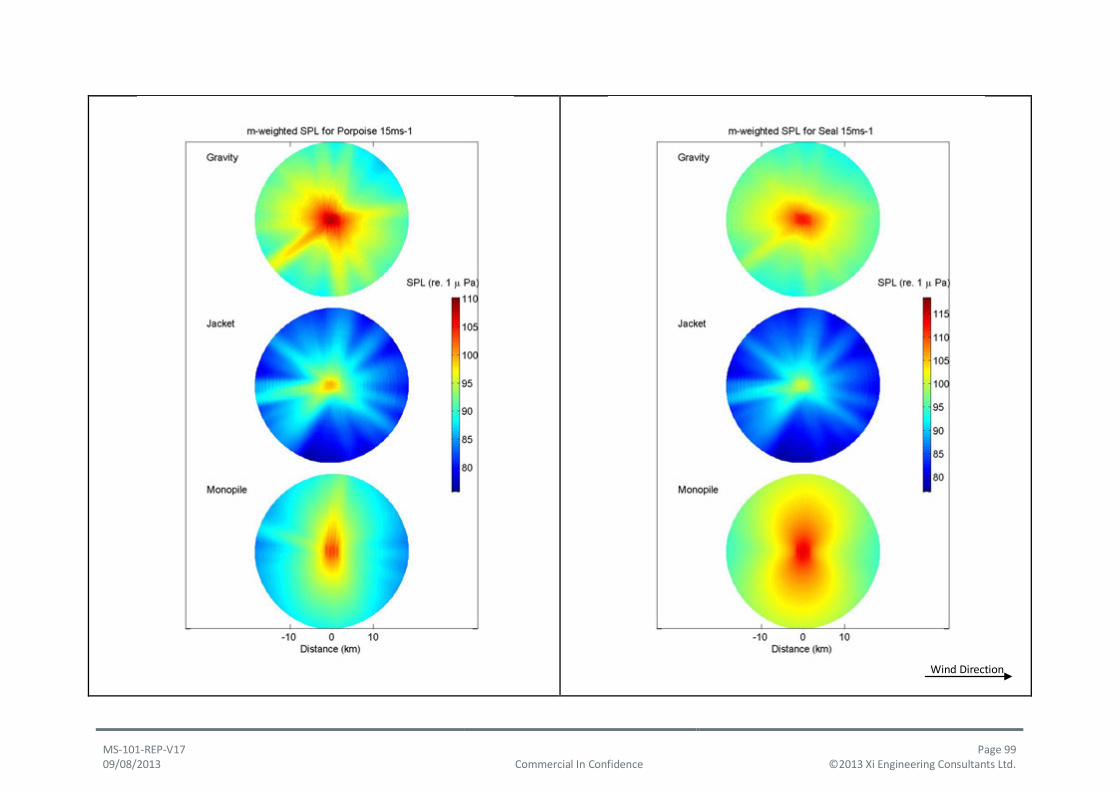
MS-101-REP-V17 Page 99 09/08/2013 Commercial In Confidence ©2013 Xi Engineering Consultants Ltd.
Wind Direction

MS-101-REP-V17 Page 100 09/08/2013 Commercial In Confidence ©2013 Xi Engineering Consultants Ltd.

w w w . s c o t l a n d . g o v . u k
© Crown copyright 2013
You may re-use this information (excluding logos and images) free of charge in any format or medium, under the terms of the Open Government Licence. To view this licence, visit http://www.nationalarchives.gov.uk/doc/open-government-licence/ or e-mail: [email protected].
Where we have identified any third party copyright information you will need to obtain permission from the copyright holders concerned.
ISBN: 978-1-78256-851-3 (web only)
The Scottish GovernmentSt Andrew’s HouseEdinburghEH1 3DG
Produced for the Scottish Government by APS Group ScotlandDPPAS14628 (08/13)
Published by the Scottish Government, August 2013