modelling of nonlinear power amplifiers for wireless...

AB HELSINKI UNIVERSITY OF TECHNOLOGY

Department of Electrical and Communications Engineering

Peter Jantunen

Modelling of Nonlinear Power Amplifiers for Wireless Communications

The thesis has been submitted for official examination for the degree of

Master of Science in Espoo, Finland on March 5th, 2004.

Supervisor Professor Timo Laakso

TEKNILLINEN KORKEAKOULU Diplomityön tiivistelmä

Tekijä: Peter Jantunen

Työn nimi: Tehovahvistimien epälineaarisuuksien mallintaminen

matkaviestinjärjestelmissä

Päivämäärä: 5.3.2004 Sivumäärä: 123

Osasto: Sähkö- ja tietoliikennetekniikan osasto

Professuuri: Signaalinkäsittelytekniikka

Työn valvoja: Professori Timo Laakso

Työn ohjaaja: Professori Timo Laakso

Tehovahvistimen epälineaarisuus vääristää lähetettävää signaalia useilla eri ta-

voilla. Tämän diplomityön tavoitteena on mallintaa tehovahvistimen epälineaa-

risuutta, jotta vahvistimen aiheuttamaa vääristymää voidaan pienentää, esimer-

kiksi linearisointitekniikoiden avulla.

Aluksi diplomityössä tarkastellaan tehovahvistimen aiheuttamaa vääristymää.

Seuraavaksi käsitellään tieteellisessä kirjallisuudessa esitettyjä malleja. Lopuksi

kaksi kiinnostavaa mallia on valittu tarkempaa tutkimista varten; yksi taajuus-

riippumaton ja yksi taajuusriippuva malli.

Polynomimallia käytettiin vahvistimen taajuusriippumatonta mallintamista var-

ten. Todettiin että matala-asteiset polynomit mallintavat tarkasti vahvistimen

ominaisuuksia tietyllä taajuudella. Tyydyttäviin tuloksiin päästiin jo viidennen

asteen mallilla.

Vahvistimen taajuusriippuvaa käyttäytymistä mallinnettiin Hammerstein mallil-

la, jossa epälineaarinen lohko toteutettiin polynomimallilla ja lineaarinen loh-

ko toteutettiin FIR-suotimella. Saatu malli osoittautui erittäin tarkaksi halutul-

la taajuuskaistalla kaikilla tehotasoilla aina pohjakohinasta vahvistimen 1-dB:n

kompressiopisteeseen asti. Lisäksi estimaatiovirhe halutun kaistan ulkopuolella

osoittautui riittävän pieneksi.

Avainsanat: Tehovahvistin, epälineaarisuus, muistillisuus, polynomi-

malli, FIR approksimaatio, Hammerstein malli.

ii

HELSINKI UNIVERSITY OF TECHNOLOGY Abstract of the Master’s Thesis

Author: Peter Jantunen

Name of the Thesis: Modelling of Nonlinear Power Amplifiers for Wireless

CommunicationsDate: 5.3.2004 Pages: 123

Department: Department of Electrical and Communications

Engineering

Professorship: Signal Processing

Supervisor: Professor Timo Laakso

Instructor: Professor Timo Laakso

The nonlinearity of a power amplifier distorts the transmitted signal in several

ways. The objective of this thesis is to find a model of the power amplifier that

can be utilized for reducing its nonlinear distortion, e.g., by linearization tech-

niques.

In this thesis, the distortion characteristics of the power amplifier are first dis-

cussed. Next, the models that have already been proposed in scientific literature

are presented. Finally, two attractive models are chosen for more detailed study;

one for frequency-independent and one for frequency-dependent modelling.

A polynomial model was used for frequency-independent modelling of a power

amplifier. It was concluded that even low-order polynomials can accurately esti-

mate the characteristics of the power amplifier at a given frequency. Sufficiently

accurate results were obtained already with a fifth-order model.

The frequency-dependent behavior of the power amplifier was modelled using a

Hammerstein model, where the nonlinear static block was implemented using a

polynomial model and the linear dynamic block as an FIR filter. The obtained

model was shown to be very accurate on the desired frequency band at all power

levels from the noise floor to the 1-dB compression point. Furthermore, the esti-

mation error outside the desired band was well behaved.

Keywords: Power amplifier, nonlinearity, memory effect, polyno-

mial model, FIR approximation, Hammerstein model.

iii

Preface

The research work for this thesis was carried out in the Signal Processing Labo-

ratory at Helsinki University of Technology during the years 2003–2004. The thesis

is part of the XMIT project that was funded by Nokia.

I wish to express my gratitude to my supervisor, Professor Timo Laakso, for his

continuous encouragement, guidance and support during the course of this work. I

am also very grateful to Stefan Werner for his numerous advice and endless interest

towards my research.

My deepest and dearest thanks go to Gilda Gámez for making the required measure-

ments. I am especially grateful for her understanding, patience and support during

the long days and nights that I have spent in the lab writing the thesis.

I would like to thank all my colleagues at the lab for creating such a nice working

atmosphere. In particular, I would like to thank Mei Yen Cheong, Martin Makundi

and Matti Rintamäki for many interesting discussions. The advice and help of my

good friend Matias With is also very highly appreciated. Special thanks to Fabio

Belloni and Eugenio Delfino for the relaxing discussions not related to signal pro-

cessing. I am also grateful to Randolph Höglund and Teemu Koski for proofreading

the thesis with such great accuracy.

In addition, I wish to express my appreciation to all the people at Nokia who made

this work possible. In particular, I would like to thank Risto Kaunisto and Pauli

Seppinen for their encouraging comments.

Finally, I would like to express my deepest gratitude towards my family and all my

friends for their endless support during my studies.

Helsinki, March 5th, 2004

Peter Jantunen

iv

Contents

List of Acronyms viii

List of Figures x

List of Tables xiii

List of Symbols xiv

1 Introduction 1

1.1 Background . . . . . . . . . . . . . . . . . . . . . . . . . . . . . . . . 1

1.2 Objective and Scope . . . . . . . . . . . . . . . . . . . . . . . . . . . 2

1.3 Organization of the Text . . . . . . . . . . . . . . . . . . . . . . . . . 3

2 Amplifier Distortion 5

2.1 The Ideal Amplifier . . . . . . . . . . . . . . . . . . . . . . . . . . . . 5

2.2 Practical Amplifiers . . . . . . . . . . . . . . . . . . . . . . . . . . . . 6

2.3 Amplitude Distortion . . . . . . . . . . . . . . . . . . . . . . . . . . . 8

2.4 Phase Distortion . . . . . . . . . . . . . . . . . . . . . . . . . . . . . 15

2.5 Memoryless Nonlinearities and Nonlinearities with Memory . . . . . . 16

2.6 Two-Tone Characterization . . . . . . . . . . . . . . . . . . . . . . . . 16

2.7 Measures of Nonlinearity . . . . . . . . . . . . . . . . . . . . . . . . . 21

2.8 Effects of Amplifier Distortion . . . . . . . . . . . . . . . . . . . . . . 27

2.9 Summary . . . . . . . . . . . . . . . . . . . . . . . . . . . . . . . . . 27

3 Parameter Estimation Theory 29

3.1 Introduction . . . . . . . . . . . . . . . . . . . . . . . . . . . . . . . . 29

v

3.2 Optimality of an Estimator . . . . . . . . . . . . . . . . . . . . . . . 31

3.3 Cramer-Rao Lower Bound . . . . . . . . . . . . . . . . . . . . . . . . 32

3.4 Minimum Variance Unbiased Estimation . . . . . . . . . . . . . . . . 35

3.5 Best Linear Unbiased Estimation . . . . . . . . . . . . . . . . . . . . 38

3.6 Least-Squares Estimation . . . . . . . . . . . . . . . . . . . . . . . . 39

3.7 Summary . . . . . . . . . . . . . . . . . . . . . . . . . . . . . . . . . 42

4 Frequency-Independent Power Amplifier Models 44

4.1 Polynomial Model . . . . . . . . . . . . . . . . . . . . . . . . . . . . . 45

4.2 Saleh Model . . . . . . . . . . . . . . . . . . . . . . . . . . . . . . . . 45

4.3 Ghorbani Model . . . . . . . . . . . . . . . . . . . . . . . . . . . . . . 46

4.4 Rapp Model . . . . . . . . . . . . . . . . . . . . . . . . . . . . . . . . 48

4.5 White Model . . . . . . . . . . . . . . . . . . . . . . . . . . . . . . . 49

4.6 Simulation Model for Memoryless Bandpass Amplifiers . . . . . . . . 50

4.7 Summary . . . . . . . . . . . . . . . . . . . . . . . . . . . . . . . . . 52

5 Frequency-Dependent Power Amplifier Models 54

5.1 Volterra Series . . . . . . . . . . . . . . . . . . . . . . . . . . . . . . . 55

5.2 Hammerstein Model . . . . . . . . . . . . . . . . . . . . . . . . . . . 58

5.3 Wiener Model . . . . . . . . . . . . . . . . . . . . . . . . . . . . . . . 61

5.4 Saleh Model . . . . . . . . . . . . . . . . . . . . . . . . . . . . . . . . 62

5.5 Summary . . . . . . . . . . . . . . . . . . . . . . . . . . . . . . . . . 63

6 Frequency-Independent Estimation of Power Amplifier

Nonlinearity Using the Polynomial Model 66

6.1 Measurement Results . . . . . . . . . . . . . . . . . . . . . . . . . . . 67

6.2 Least-Squares Estimation of the Polynomial Model Coefficients . . . . 70

6.3 Estimation Results . . . . . . . . . . . . . . . . . . . . . . . . . . . . 75

6.4 Summary . . . . . . . . . . . . . . . . . . . . . . . . . . . . . . . . . 78

7 Frequency-Dependent Estimation of Power Amplifier

Nonlinearity Using the Hammerstein Model 80

7.1 Implementation of the Hammerstein Model . . . . . . . . . . . . . . . 81

vi

7.2 Simplified Parameter Estimation of the Hammerstein Model . . . . . 82

7.3 Weighted Least-Squares FIR Approximation . . . . . . . . . . . . . . 87

7.4 Estimation Results . . . . . . . . . . . . . . . . . . . . . . . . . . . . 91

7.5 Summary . . . . . . . . . . . . . . . . . . . . . . . . . . . . . . . . . 107

8 Conclusions and Future Work 108

A Weighted Least-Squares FIR Approximation 110

B Matlab implementation of the Weighted Least-Squares FIR

Approximation 115

Bibliography 117

vii

List of Acronyms

ACPR Adjacent Channel Power Ratio

AM/AM Amplitude Modulation/Amplitude Modulation

AM/PM Amplitude Modulation/Phase Modulation

AWGN Additive White Gaussian Noise

BJT Bipolar Junction Transistor

BLB Barankin Lower Bound

BLUE Best Linear Unbiased Estimator

CRLB Cramer-Rao Lower Bound

DC Direct Current

FIR Finite Impulse-Response

IDFT Inverse Discrete Fourier Transform

IIR Infinite Impulse-Response

IM Intermodulation

IP Internet Protocol

LLF Log-Likelihood Function

LS Least-Squares

LSE Least-Squares Estimator

LTI Linear Time-Invariant

MIMR Multitone Intermodulation Ratio

MMSEE Minimum Mean Square Error Estimator

MSE Mean Square Error

MVUE Minimum Variance Unbiased Estimator

viii

NPR Noise Power Ratio

OFDM Orthogonal Frequency Division Multiplexing

PAPR Peak-to-Average Power Ratio

PDF Probability Density Function

RMS Root-Mean-Square

SSPA Solid State Power Amplifier

TWTA Traveling-Wave Tube Amplifier

VNA Vector Network Analyzer

WLSE Weighted Least-Squares Estimator

WWLB Weiss-Weinstein Lower Bound

ZZLB Ziv-Zakai Lower Bound

ix

List of Figures

1.1 Organization of the thesis. . . . . . . . . . . . . . . . . . . . . . . . . 4

2.1 Illustration of a linear operator. . . . . . . . . . . . . . . . . . . . . . 6

2.2 The ideal amplifier compared to a real amplifier. . . . . . . . . . . . . 7

2.3 Second-order and third-order input-output characteristics. . . . . . . 9

2.4 Frequency domain characteristics of a second-order nonlinearity. . . . 9

2.5 Frequency domain characteristics of a third-order nonlinearity. . . . . 11

2.6 Frequency responses of 4th- and 5th-order nonlinearities, showing sep-

arate components from different degrees of nonlinearity. . . . . . . . . 14

2.7 Illustration of a two-tone excitation. . . . . . . . . . . . . . . . . . . . 18

2.8 Time and frequency domain plots of the output of a third-order non-

linear system. . . . . . . . . . . . . . . . . . . . . . . . . . . . . . . . 20

2.9 Illustration of the 1 dB compression point. . . . . . . . . . . . . . . . 22

2.10 Illustration of the second-order and third-order intercept points. . . . 23

2.11 Amplitude and phase distortion caused by a third-order nonlinearity. 24

2.12 Illustration of nonlinearity measures for multitone and modulated

signals. . . . . . . . . . . . . . . . . . . . . . . . . . . . . . . . . . . . 26

3.1 Probability density function dependency of the estimator value ξ. . . 30

3.2 Illustration of the optimality criterions of estimators. . . . . . . . . . 32

4.1 Illustration of amplitude and phase conversion characteristics of fre-

quency independent amplifier models. . . . . . . . . . . . . . . . . . . 47

4.2 Simulation model for bandpass nonlinearities. . . . . . . . . . . . . . 51

4.3 Quadrature form simulation model for bandpass nonlinearities. . . . . 53

x

5.1 Block diagram interpretation of the Volterra series expansion. . . . . 56

5.2 Illustration of a 2nd-order Volterra filter of length 2. . . . . . . . . . . 57

5.3 Hammerstein model. . . . . . . . . . . . . . . . . . . . . . . . . . . . 58

5.4 Block diagram of a linear dynamic system. . . . . . . . . . . . . . . . 59

5.5 Wiener model. . . . . . . . . . . . . . . . . . . . . . . . . . . . . . . . 61

5.6 The frequency-dependent Saleh model. . . . . . . . . . . . . . . . . . 64

6.1 Mini-Circuits ZVE-8G power amplifier with standard heat sink at-

tached. . . . . . . . . . . . . . . . . . . . . . . . . . . . . . . . . . . . 67

6.2 Single-tone measurement setup for AM/AM and AM/PM measure-

ments. . . . . . . . . . . . . . . . . . . . . . . . . . . . . . . . . . . . 68

6.3 Measured amplitude and phase response of the Mini-Circuits ZVE-8G

power amplifier at selected power levels. . . . . . . . . . . . . . . . . 69

6.4 Measured amplitude and phase conversion characteristics of the Mini-

Circuits ZVE-8G power amplifier at selected frequencies. . . . . . . . 71

6.5 A 5th-order least-squares polynomial fit of the measured AM/AM

and AM/PM characteristics at 6 GHz. . . . . . . . . . . . . . . . . . 76

6.6 Estimation error of the polynomial model as a function of the order

of the polynomial. . . . . . . . . . . . . . . . . . . . . . . . . . . . . . 77

6.7 Difference between the measured AM/AM & AM/PM and the esti-

mated AM/AM & AM/PM characteristics of 5th-order polynomials

fitted to selected frequencies. . . . . . . . . . . . . . . . . . . . . . . . 78

7.1 Block diagram of the frequency-dependent estimation problem for the

Hammerstein model. . . . . . . . . . . . . . . . . . . . . . . . . . . . 81

7.2 Illustration of the minimum sampling rate for the FIR filter design. . 87

7.3 A first direct form realization of an causal Mth-order FIR filter. . . . 88

7.4 Frequency response of FIR filters designed using weighted least-squares

FIR approximation. . . . . . . . . . . . . . . . . . . . . . . . . . . . . 92

7.5 Illustration of the filter characteristics obtained using weighted least-

squares FIR approximation. . . . . . . . . . . . . . . . . . . . . . . . 93

xi

7.6 Relative least-squares error of the weighted least-squares FIR approx-

imation as a function of the filter order. . . . . . . . . . . . . . . . . . 94

7.7 FIR filters of selected orders fitted to the measured small-signal ampli-

tude and phase response of the Mini-Circuits ZVE-8G power amplifier. 96

7.8 Illustration of the effect of the weighting factor on the estimation

accuracy. . . . . . . . . . . . . . . . . . . . . . . . . . . . . . . . . . . 97

7.9 Estimation accuracy of the weighted least-squares FIR approximation. 98

7.10 Implementation of the Hammerstein model. . . . . . . . . . . . . . . 99

7.11 A comparison between the measured and estimated amplitude re-

sponse at –27 dBm and 0 dBm input power levels . . . . . . . . . . . 100

7.12 A comparison between the measured and estimated phase response

at –27 dBm and 0 dBm input power levels. . . . . . . . . . . . . . . . 101

7.13 A comparison between the measured and estimated AM/AM charac-

teristics at selected frequencies. . . . . . . . . . . . . . . . . . . . . . 103

7.14 A comparison between the measured and estimated AM/PM charac-

teristics at selected frequencies. . . . . . . . . . . . . . . . . . . . . . 104

7.15 Illustration of the Hammerstein model estimation error. . . . . . . . . 106

xii

List of Tables

2.1 Distortion effects generated by frequency-independent and frequency-

dependent nonlinear amplifiers. . . . . . . . . . . . . . . . . . . . . . 17

2.2 Frequency components generated by a third-order nonlinear system. . 19

2.3 List of frequency components generated by a third-order nonlinearity. 21

5.1 Mapping between the original parameters and the linearized param-

eters of the Hammerstein system described in Equations (5.11) and

(5.12). . . . . . . . . . . . . . . . . . . . . . . . . . . . . . . . . . . . 60

6.1 Mini-Circuits ZVE-8G specifications. . . . . . . . . . . . . . . . . . . 67

7.1 Proposed technique for simplified parameter estimation of the Ham-

merstein model. . . . . . . . . . . . . . . . . . . . . . . . . . . . . . . 85

xiii

List of Symbols

ξ estimator

σ standard deviation

τ time delay

Φ phase conversion function

φ phase

φd,l desired output phase values

φds,l scaled desired output phase values

φout output phase shift

Ψ nonlinear conversion function

ω angular frequency

ωc center frequency of the desired band

A amplitude

Ad,l desired output amplitude values

As input amplitude level of the measured small-signal frequency response

a coefficient vector of gain conversion polynomial

b coefficient vector of phase conversion polynomial

C covariance matrix

D filter delay

E error function

e error signal

e discrete-time Fourier transform vector

F Fisher information matrix

xiv

f frequency

fs sampling frequency

G voltage gain

g gain conversion function

H frequency response

Hd desired frequency response

Hd,p desired power-dependent frequency response

Hd,s small-signal frequency response

Hd,s0scaled small-signal frequency response

Hp estimated power-dependent frequency response

h filter coefficient vector

I identity matrix

K number of measured frequency points

L number of measured amplitude levels

M filter order

N order of the nonlinearity

N Gaussian probability density function

pin input power values

pout output power values

Q amplifier operating point

R whitening matrix

s signal model

t time

U observation matrix

Vin input voltage

Vout output voltage

W weighting matrix

w noise vector

Wf weighting factor

x input signal

y output signal

xv

Chapter 1

Introduction

1.1 Background

The major driver for future wireless broadband multimedia communication systems

is the increasing demand for personal mobile communications that require increased

data rates, capacity, flexibility and reliability. Users are expecting mobile Internet

Protocol (IP) applications and services comparable to fixed line applications and

services at home or in the office. The new radio interfaces are predicted to support

data rates up to 100 Mbit/s for mobile access and up to 1 Gbit/s for wireless local

area access [1]. This means that the limited bandwidth, transmit power and other

resources must be used as efficiently as possible, close to the optimal theoretical

limits.

Orthogonal Frequency Division Multiplexing (OFDM) is one of the most promising

modulation technologies for these future systems. OFDM is a multicarrier modu-

lation technique where a single data stream is transmitted over a number of lower

rate subcarriers. Some of the key advantages of OFDM are efficient handling of

multipath environments, channel capacity enhancement in slow time-varying chan-

nels, robustness against narrowband interference and high spectral efficiency. The

1

most notable drawbacks are the high Peak-to-Average Power Ratio (PAPR) and

sensitivity to both frequency offset and phase noise.

High PAPR indicates that a highly linear power amplifier is required at the trans-

mitter. The linearity requirement can be met by driving the power amplifier well

below its saturation point. This causes poor power efficiency, which is especially

bad in a mobile transmitter. Driving the power amplifier closer to its saturation

point is appealing, since it would increase power efficiency and prolong battery life

of a mobile transmitter. However, driving the power amplifier above the linear re-

gion results in nonlinear distortion effects. The nonlinear distortion makes it more

difficult to receive the signal and generates harmonic and intermodulation signals

outside of the intended frequency band. These unwanted distortion products are

potential interfering sources to other users of the radio interface, especially on adja-

cent frequency bands. The interference must therefore be reduced to a level where

both systems can operate satisfactorily.

1.2 Objective and Scope

The goal of this thesis is to find a model for the power amplifier that can be utilized

by linearization techniques in order to reduce the nonlinear distortion caused by the

power amplifier. Narrowband amplifiers can usually be characterized by frequency-

independent models, while wideband amplifiers require frequency-dependent mod-

els. Frequency-independent models can easily be obtained using polynomials, since

estimation of the coefficients of the polynomials can be done using linear param-

eter estimation techniques. Frequency-dependent models are much more complex

to obtain, since usually nonlinear estimation techniques must be used. Therefore,

simplified block models that split the nonlinearity and the dynamics of the system

have been shown to be more promising.

The objective is to find both a frequency-independent and a frequency-dependent

model that can be used for modelling different types of amplifiers, that are used in

2

various applications and environments. Preferably, it should be possible to model

the nonlinearity of the frequency-dependent model using the frequency-independent

model. Hence, the more simple frequency-independent model can be first evaluated,

and if satisfactory results cannot be obtained, it is easy to extend it with a frequency-

dependent block.

1.3 Organization of the Text

The outline of the thesis is illustrated in Figure 1.1. The thesis can be divided into

two parts, where Chapters 2–5 consist of the literature study and the theoretical

background and Chapters 6–7 consist of my own contribution to identification of

nonlinear systems.

Chapter 2 describes how an amplifier distorts the transmitted signal, how the dis-

tortion can be measured, and what are the effects of the distortion. The differ-

ence of memoryless nonlinearities and nonlinearities with memory is also discussed.

Chapter 3 provides background on the parameter estimation theory required for de-

termining the unknown coefficients of the power amplifier models. The focus is on

linear parameter estimation techniques. Chapters 4 and 5 discuss the most widely

used frequency-independent and frequency-dependent power amplifier models found

in the scientific literature.

In the two following chapters, the models presented in Chapters 4 and 5 are ap-

plied for modelling a practical wideband power amplifier. Chapter 6 presents the

estimation results using a frequency-independent polynomial model and Chapter 7

presents the estimation results using a frequency-dependent Hammerstein model.

In addition, Chapter 7 presents a simplified parameter estimation technique for sep-

arately determining the coefficients of the two blocks of the Hammerstein model.

Furthermore, a design technique for Finite Impulse-Response (FIR) filters that can

have arbitrary amplitude and phase response is derived. Finally, Chapter 8 presents

the conclusions and some suggestions for future work.

3

Chapter 1Introduction

Theoretical Aspects

Chapter 2Amplifier Distortion

Chapter 3Parameter Estimation Theory

Amplifier Models

Chapter 4Frequency IndependentPower Amplifier Models

Chapter 5Frequency Dependent

Power Amplifier Models

Chapter 6Frequency-Independent Estimation of Power Amplifier Nonlinearity

Using the Polynomial Model

Chapter 7Frequency-Dependent Estimation of Power Amplifier Nonlinearity

Using the Hammerstein Model

Chapter 8Conclusions and Future Work

Figure 1.1: Organization of the thesis.

4

Chapter 2

Amplifier Distortion

All amplifiers distort the signals that they are intended to amplify. The distortion

impairs the transmitted signal, which makes it more difficult to receive the trans-

mission correctly. The distortion may not only present problems for users in the

same channel but also for users in adjacent channels. This chapter defines what

distortion is, what its measures are and what are the effects of the distortion.

2.1 The Ideal Amplifier

An ideal amplifier would produce as its output a perfect replica of the input multi-

plied by a scalar value. The linear transfer characteristics can be written as

Vout(t) = GVin(t) (2.1)

where G is the voltage gain of the amplifier. Mathematically, an operator L is said

to be linear if the scaling and superposition principles

L(αx1) = αL(x1) (2.2a)

L(x1 + x2) = L(x1) + L(x2) (2.2b)

5

L (·)x y

Figure 2.1: Illustration of a linear operator.

hold for every pair of functions x1 and x2 and scalar α [2]. The linear operator

is illustrated in Figure 2.1. The linearity implies that the ideal amplifier does not

affect the waveform of the transmitted signal nor does it introduce any new frequency

components. The ideal amplifier is illustrated in Figure 2.2(a).

2.2 Practical Amplifiers

Real amplifiers exhibit various magnitudes of nonlinearities. These are usually de-

scribed by the amplitude transfer characteristics and the phase transfer character-

istics of the amplifier. The first one is often also referred to as the Amplitude

Modulation/Amplitude Modulation (AM/AM) conversion and the latter one as the

Amplitude Modulation/Phase Modulation (AM/PM) conversion of the amplifier.

A comparison between a real amplifier and its ideal counterpart is shown in Figure

2.2. The figure shows that there are significant differences between the two ampli-

fiers. The real amplifier illustrated in Figure 2.2(b) has three different operating

regions. When the input signal voltage is low, the amplifier is operating in the

cutoff region and the input-output relationship has an exponential form. In the

linear region the amplifier performs almost as its ideal counterpart until the input

rises high enough, so that the output saturates to the maximum output level. The

label Q is the quiescent point often also referred to as the Direct Current (DC)

bias or the operating point of the amplifier. More detailed information on operation

characteristics of real amplifiers can be found in [3].

The nonlinearity depicted in Figure 2.2(b) shows that the saturation of the amplifier

has smoothly decreased the amplitude of the output signal’s upper half. Besides the

AM/AM conversion shown in the figure, real amplifiers may also cause AM/PM

6

−0.2 0 0.2 0.4 0.6 0.8 1 1.2−2

0

2

4

6

8

10

12

← Input signal

Output signal →

Input voltage Vin

Outp

ut

volt

age

Vout

Q

(a) Ideal amplifier with voltage gain G = 20.

−0.2 0 0.2 0.4 0.6 0.8 1 1.2−2

0

2

4

6

8

10

12

← Input signal

Output signal →

Input voltage Vin

Outp

ut

volt

age

Vout

Cutoff region Linear region Saturation region

Q

(b) Real amplifier with voltage gain G = 20 in the linear region.

Figure 2.2: Comparison between an ideal amplifier and a real amplifier. Q is theoperating point of the amplifier.

7

conversion and both the AM/AM and AM/PM characteristics may also depend on

the input signal frequency.

2.3 Amplitude Distortion

2.3.1 Second-order Nonlinearity

Since no physical device can act as the ideal amplifier illustrated in Figure 2.2(a),

models for nonlinear amplifiers are needed. The simplest nonlinearity can be il-

lustrated by adding a squared term to the input-output relationship of the ideal

amplifier in Equation (2.1). The input-output relationship is now written as

Vout(t) = G1Vin(t) + G2V2in(t). (2.3)

Using a sinusoidal input

Vin(t) = A(ω) cos(ωt) (2.4)

the output of the nonlinear amplifier can be calculated using basic trigonometric

identities

Vout(t) = G1A(ω) cos(ωt) + G2A2(ω) cos2(ωt)

= G1A(ω) cos(ωt) + G2A2(ω)

1 + cos(2ωt)

2

=G2A

2(ω)

2+ G1A(ω) cos(ωt) +

G2A2(ω)

2cos(2ωt).

(2.5)

The input-output relationship of the second-order nonlinearity is illustrated in Fig-

ure 2.3(a) using G1 = 10, G2 = 4 and A = 1. Equation (2.5) shows that the second

order nonlinearity introduces a DC component and a new signal component at twice

the frequency of the fundamental component. This is illustrated in Figure 2.4. Since

the fundamental component is not affected by the nonlinearity, the distortion can

be removed by filtering.

8

−0.2 0 0.2 0.4 0.6 0.8 1 1.2−2

0

2

4

6

8

10

12

Real amplifier2nd−order model

Input voltage Vin

Outp

ut

volt

age

Vout

(a) Vout(t) = 10Vin(t) + 4V 2

in(t)

−0.2 0 0.2 0.4 0.6 0.8 1 1.2−2

0

2

4

6

8

10

12

Real amplifier3rd−order model

Input voltage Vin

Outp

ut

volt

age

Vout

(b) Vout(t) = 13Vin(t)− 3V 3

in(t)

Figure 2.3: Second-order and third-order nonlinear input-output characteristicscompared to the real amplifier illustrated in Figure 2.2(b). The input signal isVin(t) = cos(ωt).

0 f 2f−2

0

2

4

6

8

10

12

Frequency

Am

plitu

de

(a) Input signal

0 f 2f−2

0

2

4

6

8

10

12

Frequency

Am

plitu

de

(b) Output signal

Figure 2.4: Frequency domain characteristics of a second-order nonlinearity Vout(t) =10Vin(t) + 4V 2

in(t), Vin(t) = cos(ωt).

9

2.3.2 Third-order Nonlinearity

Adding a third-order term to the input-output relationship of the ideal amplifier in

Equation (2.1) gives a very different set of problems compared to the second order

nonlinearity. The input-output relationship of the nonlinear amplifier is now

Vout(t) = G1Vin(t) + G3V3in(t). (2.6)

Using the sinusoidal input defined in Equation (2.4), it is easy to calculate the output

of the amplifier

Vout(t) = G1A(ω) cos(ωt) + G3A3(ω) cos3(ωt)

= (G1A(ω) +3G3A

3(ω)

4) cos(ωt) +

G3A3(ω)

4cos(3ωt).

(2.7)

The third-order input-output relationship is illustrated in Figure 2.3(b) using G1 =

13, G3 = −3 and A = 1. With the third-order nonlinearity, the amplifier produces

a new signal component with three times the frequency of the fundamental com-

ponent. There is no DC component, but instead, the fundamental component has

been multiplied by a factor proportional to the cube of the input amplitude. The

frequency domain transfer characteristics are illustrated in Figure 2.5.

The most notable difference between the second-order and the third-order nonlin-

earity is that the latter produces in-band distortion which cannot be filtered away.

This can be verified by looking at the example plotted in Figure 2.5. The transfer

function indicates that the fundamental component should have an output ampli-

tude of 13 times the input signal amplitude, but from Figure 2.5(b) it can be seen

that the output signal only has an amplitude of 10.75 V. This is because the third

order nonlinearity produces a component at the fundamental frequency with an am-

plitude of -2.25 V, so that the final output amplitude becomes only 10.75 V instead

of 13 V.

10

1 3f−2

0

2

4

6

8

10

12

Frequency

Am

plitu

de

(a) Input signal

1 3f−2

0

2

4

6

8

10

12

Frequency

Am

plitu

de

(b) Output signal

Figure 2.5: Frequency domain characteristics of a third-order nonlinearity Vout(t) =13Vin(t)− 3V 3

in(t), Vin(t) = cos(ωt).

2.3.3 Higher-order Nonlinearities

Sections 2.3.1 and 2.3.2 showed that the characteristics of the nonlinearity are very

different depending on the order of the nonlinearity. The results of these sections

can be generalized for even-order and odd-order nonlinearities.

Even-order Nonlinearities

An Nth-order even-order nonlinearity can be characterized by the relationship

Vout(t) =

N/2∑

n=0

G2nV 2nin . (2.8)

Using the input defined in Equation (2.4) the output of the amplifier is

Vout(t) = G0 +

N/2∑

n=1

G2nA2n(ω) cos2n(ωt). (2.9)

11

Expanding the cosine term at the output using (Id. 8, Sec. 5.4 in [4])

cos2n(ωt) =

(2n

n

)1

22n+

1

22n−1

n∑

k=1

(2n

n− k

)

cos(2kωt) (2.10)

the output of the even-order nonlinearity can be evaluated as

Vout(t) = G0 +

N/2∑

n=1

(2n

n

)G2nA2n(ω)

22n

+

N/2∑

n=1

G2nA2n(ω)

22n−1

n∑

k=1

(2n

n− k

)

cos(2kωt).

(2.11)

Equation (2.11) shows that an even-order nonlinearity leaves the fundamental com-

ponent unchanged, but produces harmonic components at even multiples of the

fundamental frequency up to the order of the nonlinearity. It also adds a DC com-

ponent to the output. This means that all even-order nonlinearities can be mitigated

by filtering.

The frequency domain characteristics of an even-order nonlinearity can be illustrated

using the 4th-order input-output relationship

Vout(t) = G0 + G1Vin(t) + G2V2in(t) + G4V

4in(t). (2.12)

Using the input from Equation (2.4) and expanding the output using Equation

(2.11), the result is

Vout(t) =8G0 + 4G2A

2(ω) + 3G4A4(ω)

8

+ G1A(ω) cos(ωt)

+G2A

2(ω) + G4A4(ω)

2cos(2ωt)

+G4A

4(ω)

8cos(4ωt).

(2.13)

12

The different frequency components in Equation (2.13) have been plotted in Figure

2.6(a), using G0 = 0, G1 = 1, G2 = G4 = 1 and A = 1.

Odd-order Nonlinearities

The Nth-order odd-order nonlinearity can be written as

Vout(t) =

(N+1)/2∑

n=1

G2n−1V2n−1in . (2.14)

Using the input defined in Equation (2.4) the output of the amplifier is

Vout(t) =

(N+1)/2∑

n=1

G2n−1A2n−1(ω) cos2n−1(ωt). (2.15)

The cosine term can be expanded using (Id. 8, Sec 5.4 in [4])

cos2n−1(ωt) =1

22n−2

n∑

k=1

(2n− 1

n− k

)

cos[(2k − 1)ωt] (2.16)

and therefore the output can be evaluated as

Vout(t) =

(N+1)/2∑

n=1

G2n−1A2n−1(ω)

22n−2

n∑

k=1

(2n− 1

n− k

)

cos[(2k − 1)ωt]. (2.17)

13

0 f 2f 3f 4f 5f 6f0

0.2

0.4

0.6

0.8

11

2 2, 4

4

4

Frequency

Am

plitu

de

(a) Vout(t) = Vin(t) + V 2

in(t) + V 4

in(t)

0 f 2f 3f 4f 5f 6f0

0.2

0.4

0.6

0.8

11

3

3

5

5

5

Frequency

Am

plitu

de

(b) Vout(t) = Vin(t) + V 3

in(t) + V 5

in(t)

Figure 2.6: Frequency responses of 4th- and 5th-order nonlinearities, showing sepa-rate components from different degrees of nonlinearity.

14

Equation (2.17) shows that the odd-order nonlinearity produces harmonic compo-

nents at odd multiples of the fundamental frequency up to the order of the nonlin-

earity. A major difference to the even-order nonlinearity is that the amplitude of

the fundamental frequency has been changed. This can be illustrated by considering

a 5th-order nonlinearity

Vout(t) = G1Vin(t) + G3V3in(t) + G5V

5in(t). (2.18)

Using the input from Equation (2.4) and expanding the output using Equation (2.17)

yields

Vout(t) =16G1A(ω) + 12G3A

3(ω) + 10G5A5(ω)

16cos(ωt)

+4G3A

3(ω) + 5G5A5(ω)

16cos(3ωt)

+G5A

5(ω)

16cos(5ωt).

(2.19)

This result verifies that an odd-order nonlinearity produces odd-order harmonics and

that the amplitude of the fundamental frequency has been multiplied by coefficients

from the higher-order components of the transfer function. The result is illustrated

in Figure 2.6(b), using G1 = G2 = G3 = 1 and A = 1.

2.4 Phase Distortion

Phase distortion occurs when an amplifier does not delay all frequency components

by the same amount. Different time delays distort a waveform consisting of several

sinusoids. The relationship between the time delay and phase shift can be written

as

τ =φ

2πf(2.20)

where τ is the time delay, φ is the phase shift and f is the fundamental frequency

of the waveform [5]. The equation clearly shows that if the phase does not increase

linearly with the frequency the time delay will vary between different frequencies.

15

2.5 Memoryless Nonlinearities and Nonlinearities

with Memory

The output of a memoryless system is a function of the input at a given time instant

or after a fixed time delay. Any change in the input occurs instantaneously at the

output. This means that the system cannot include any energy storing components

which implies that the output is in-phase with the input. In frequency domain

the zero-memory nonlinearity implies that the transfer characteristics are frequency

independent.

In systems with memory the output of the system also depends on the previous input

values. This means that the system includes energy storing components. Besides

gain distortion, a nonlinear system with memory may also cause phase distortion.

Furthermore, both the gain and phase distortion may be frequency-dependent. A

detailed discussion of nonlinearities with and without memory can be found in [6,7].

Memoryless amplifiers are an idealization since practical amplifiers include energy

storing components. Therefore the memory of a system is not a good criterion for

classifying amplifiers. A more natural approach is to denote amplifiers as frequency-

independent or frequency-dependent systems. A frequency-independent system can

be either a memoryless system or a system with memory. Frequency-dependent

systems on the other hand are always systems with memory. The distortion effects

generated by frequency-independent and frequency-dependent nonlinear amplifiers

are summarized in Table 2.1.

2.6 Two-Tone Characterization

Two-tone characterization can illustrate both amplitude and phase distortions present

in an amplifier. In a two-tone test the amplifier is fed by a signal of the form

Vin = A1 cos(ω1t) + A2 cos(ω2t). (2.21)

16

Table 2.1: Distortion effects generated by frequency-independent and frequency-dependent nonlinear amplifiers.

Frequency-Independent Systems Frequency-Dependent SystemsMemoryless Systems: Systems with Memory:• Gain Distortion • Frequency-Dependent Gain DistortionSystems with Memory: • Frequency-Dependent Phase Distortion• Gain Distortion• Phase Distortion

Figure 2.7 illustrates the signal in both frequency and time domain. The frequency

domain plot is an idealization, since it only shows two sinusoids. In practice there

would be small frequency components caused by the nonlinearities of the signal

generator. The time domain plot reveals that the input signal can be set to vary

throughout the whole dynamic range of the amplifier.

2.6.1 Frequency Generation

The two-tone input to a nonlinear device produces new frequency components at

the output of the device. The new components occur at linear combinations of the

two excitation frequencies. The generated frequencies are of the form

ωm,n = mω1 + nω2 (2.22)

where m and n are positive or negative integers and |m| + |n| ≤ N where N is the

order of the nonlinearity. [8]

2.6.2 A Third-order System

A third-order system Vout = G0 + G1Vin + G2V2in + G3V

3in generates frequency com-

ponents illustrated in Table 2.2. The linear term G1 amplifies the fundamental

components ω1 and ω2. The quadratic term G2 converts the signal down to the DC

17

0

0.2

0.4

0.6

0.8

1

1.2

1.4

1.6

1.8

2

0 f1 f2 2f1Frequency

Am

plitu

de

(a) Two-tone excitation in the frequency domain.

0 20 40 60 80 100 120−2

−1.5

−1

−0.5

0

0.5

1

1.5

2

Time

Am

plitu

de

(b) Two-tone excitation in the time domain.

Figure 2.7: Illustration of a two-tone excitation.

18

Table 2.2: Frequency components generated by the nonlinear input-output relation-ship Vout = G0 + G1Vin + G2V

2in + G3V

3in, where Vin is a two tone excitation.

Frequency Amplitude Frequency Amplitude

0 G0 + G2A2 ω1 + ω2 G2A

2

ω2 − ω1 G2A2 2ω2

G2A2

2

2ω1 − ω23G3A3

43ω1

G3A3

4

ω14G1A+9G3A3

42ω1 + ω2

3G3A3

4

ω24G1A+9G3A3

42ω2 + ω1

3G3A3

4

2ω2 − ω13G3A3

43ω2

G3A3

4

2ω1G2A2

2

band to the frequencies 0 Hz and ω2−ω1. It also creates the second harmonic band

with components 2ω1, 2ω2 and ω1 + ω2. The cubic term G3 creates the third-order

intermodulation components 2ω1 − ω2 and 2ω2 − ω1, the compression or expansion

terms on top of the fundamental tones ω1 and ω2, and also the third harmonic band

with components 3ω1, 2ω1 + ω2, 2ω2 + ω1 and 3ω2.

The third-order system is further illustrated in Figure 2.8, where the output of the

transfer function Vout = 2+10Vin +V 2in− 3V 3

in is plotted in both time and frequency

domain. The input signal is Vin = 0.5 cos(0.95t) + 0.5 cos(1.05t). The frequency

domain plot clearly shows the different frequency bands created by the nonlinearity.

The output amplitude values of the frequency plot are listed in Table 2.3.

2.6.3 Nonlinear Phenomena

The generated frequency components can be roughly grouped into two categories,

namely the harmonic components and the intermodulation (IM) components. In

communication systems the harmonics may interfere with other systems and must

therefore be reduced by filters or by other means. This is not a major problem since

the harmonics occur at frequencies high above the desired frequency, so that the

filtering can be quite easily performed.

19

−0.2 0 0.2 0.4 0.6 0.8 1 1.2−2

0

2

4

6

8

10

12

Input Voltage

Outp

ut

Vol

tage

(a)

−3

−2

−1

0

1

2

3

4

0 ω2 −

ω1

2ω1 −

ω2

ω1

ω22ω

2 −ω1

2ω1

ω1 +

ω2

2ω2

3ω1

2ω1 +

ω2

2ω2 +

ω1

3ω2

Am

plitu

de

(b)

Figure 2.8: Time and frequency domain plots of the output of a third-order nonlinearsystem Vout = 2 + 10Vin + V 2

in − 3V 3in using a two-tone input Vin = cos(0.95t) +

cos(1.05t). The amplitude values are listed in Table 2.3.

20

Table 2.3: List of frequency components generated by the nonlinear input-outputrelationship Vout = 2 + 10Vin + V 2

in − 3V 3in, where Vin = cos(0.95t) + cos(1.05t).

Frequency Amplitude Frequency Amplitude

0 3.00 ω1 + ω2 3.00ω2 − ω1 3.00 2ω2 0.502ω1 − ω2 −2.25 3ω1 −0.75

ω1 3.25 2ω1 + ω2 −2.25ω2 3.25 2ω2 + ω1 −2.25

2ω2 − ω1 −2.25 3ω2 −0.752ω1 0.50

The intermodulation components on the other hand often pose a more serious prob-

lem, because some of them appear in-band and can be mistaken for desired signals.

The even-order IM products are not a problem since they appear at frequencies well

below or above the signals that created them. However, the odd-order IM products

present a problem, since they appear in-band. The third-order products present the

greatest problems because they are the strongest and the closest to the signals that

generated them and thus are often impossible to reject with the use of filters [8].

2.7 Measures of Nonlinearity

2.7.1 The 1-dB Compression Point

The 1-dB compression point refers to the output power level where the transfer char-

acteristics of the amplifier have dropped by 1 dB from the ideal linear characteris-

tics [5]. The 1-dB compression point of an amplifier with a third-order nonlinearity

is illustrated in Figure 2.9.

21

−12 −10 −8 −6 −4 −2 08

10

12

14

16

18

20

22

24

Real Transfer CharacteristicsIdeal Transfer Characteristics

l 1 dB

1 dBCompression Point

Input Power (dBm)

Outp

ut

Pow

er(d

Bm

)

Figure 2.9: Illustration of the 1 dB compression point.

2.7.2 Intercept Points

Intercept points provide a simple method for predicting the amount of nonlinear

distortion of an amplifier at a particular operating point. If the input-output rela-

tionship of a device is plotted on a log-log scale, the slope of the linear component

will be 1. If the second-order distortion products are shown on the same scale, they

will have a slope of 2, the third order distortion products will have a slope of 3,

etc. [7]

The intercept point is the point where the linear extrapolation of the harmonic

component intersects with the linear extrapolation of the fundamental component.

The second-order and third-order intercept points of the nonlinear transfer functions

in Equations (2.3) and (2.6) are illustrated in Figure 2.10.

22

−30 −20 −10 0 10 20

−10

0

10

20

30

40

Second-order intercept point →

Fundamental →

← Second harmonic

Input Power (dBm)

Outp

ut

Pow

er(d

Bm

)

(a) Vout(t) = 10Vin(t) + 4V 2

in(t)

−30 −20 −10 0 10 20

−10

0

10

20

30

40Third-order intercept point →

Linear gain →

Fundamental →

Third harmonic →

Input Power (dBm)

Outp

ut

Pow

er(d

Bm

)

(b) Vout(t) = 13Vin(t)− 3V 3

in(t)

Figure 2.10: Illustration of the second-order and third-order intercept points.

23

(a) AM-AM compression (b) AM-AM expansion (c) AM-PM conversion(d) AM-AM andAM-PM conversion

Figure 2.11: Amplitude and phase distortion caused by a third-order nonlinearity.

2.7.3 AM-AM and AM-PM Conversion

Another widely used measure is to show the fundamental and third-order spectral

components as vectors. This is done by showing the third-order vector on top of

the fundamental vector. This is illustrated in Figure 2.11, where the vectors of the

system Vout = G1Vin + G3V3in are shown at a certain input amplitude value. The

length of the third-order vectors will grow as the input amplitude is increased.

Figure 2.11(a) shows the situation where the output signal is compressed due to the

third-order term. In this case both G1 and G3 are real and have opposite signs. If

the signs are equal, amplitude expansion will occur. This is illustrated in Figure

2.11(b). Figure 2.11(c) illustrates a 90 phase conversion. The third-order vector is

now pointing to the right and therefore the third-order term G3 must be a complex

number to model the phase shift. Figure 2.11(d) shows the situation where the

nonlinearity causes both amplitude and phase conversion. [7]

24

2.7.4 Adjacent Channel Power Ratio

Adjacent Channel Power Ratio (ACPR) is a measure of the degree of signal spreading

into adjacent channels, caused by nonlinearities in a power amplifier. It is defined

as the power contained in a defined bandwidth (B1) at a defined offset (f0) from the

channel center frequency (fc), divided by the power in a defined bandwidth (B2)

placed around the channel center frequency. This is illustrated in Figure 2.12(a). [5]

2.7.5 Noise Power Ratio

Noise Power Ratio (NPR) is a measure of the unwanted in-channel distortion power

caused by the nonlinearity of the power amplifier. It can be measured by applying

a notch filter at the center frequency of the transmission channel and examining the

level of distortion that fills the notch. NPR is defined as the ratio between the noise

power spectral density passing through the amplifier measured at the center of the

notch compared to the noise power spectral density without the notch filter. The

concept is illustrated in Figure 2.12(b). [5]

2.7.6 Multitone Intermodulation Ratio

Multitone Intermodulation Ratio (MIMR) is a measure of the effect of nonlinearity

on a multicarrier signal. It is defined as the ratio between the wanted tone power

and the highest intermodulation tone power just outside of the wanted band. This

is illustrated in Figure 2.12(c). [5]

25

fc − f0 fc

B1 B2

Frequency

Am

plitu

de

(a) Adjacent power ratio

fc

NPR

Frequency

Am

plitu

de

(b) Noise power ratio

0

2

4

6

8

10

12

fc

MIMR

Frequency

Am

plitu

de

(c) Multitone intermodulation ratio

Figure 2.12: Illustration of nonlinearity measures for multitone and modulated sig-nals [5].

26

2.8 Effects of Amplifier Distortion

The nonlinearities of the amplifier degrade the transmitted signal in several ways.

The following lists some of the most significant adverse effects.

• Additional nonlinear interference in the receiver [9]

• Spectral spreading of the transmitted signal, which can cause adjacent channel

interference [9]

• Signal constellation deformation and spreading [10,11]

• Interference between the in-phase and quadrature components due to AM/PM

conversion [9]

• Intermodulation effects, which occur, when several channels are amplified in a

single amplifier [9]

• Degradation in the antenna amplitude and phase weightings due to intermod-

ulation in adaptive antenna systems. This causes degradation to the antenna

beam pattern and null depth [5]

2.9 Summary

This chapter introduced some definitions of amplifier nonlinearities as well as cate-

gorized the nonlinearities. Measures of nonlinearities for single-tone and multitone

inputs were also illustrated. Finally some effects of the distortion were listed.

A linear system does not alter the signal waveform that passes through it. Nonlinear

systems on the other hand distort the signal due to amplitude and phase conversion.

The nonlinear system can be characterized as a memoryless system or as a system

with memory. In a memoryless system the output of the system is an instantaneous

function of the input and therefore the system cannot present any phase conversion.

27

If the system has memory, then also the previous input values affect the output.

The memory is caused by energy storing components inside the system that cannot

alter their state instantaneously.

Two-tone measurements can be used to verify the transfer characteristics of an

amplifier. A two-tone excitation fed to a nonlinear system generates harmonic bands

as well as in-band intermodulation distortion. The most serious problems are faced

due to the third-order intermodulation components, because these are the strongest

components and also the ones that are closest to the signals that generated them

and are thus often impossible to reject by filtering.

28

Chapter 3

Parameter Estimation Theory

3.1 Introduction

The subsequent chapters present models for the adverse nonlinear effects discussed

in the previous chapter. These models include unknown parameters that need to

be determined. Mathematically this can be formulated as follows. Given a set of

data x[0], x[1], · · · , x[L− 1] that depends on an unknown parameter ξ, we wish to

determine ξ based on the data or in other words to define an estimator

ξ = γ(x[0], x[1], · · · , x[L− 1]) (3.1)

where γ is some function [12]. This is the problem of parameter estimation that is

addressed in this chapter.

The estimation process begins by assuming an appropriate model for the input.

Since the data is inherently random, it is usually described by its Probability Density

Function (PDF) denoted by p(x[0], x[1], · · · , x[L−1]; ξ). The PDF is parameterized

by the unknown parameter ξ, so that changing the value of ξ yields different PDFs.

To illustrate the situation let us assume only one measurement data point, i.e., L = 1

29

x[0]

p(x[0

];ξ)

E [ξ1] E [ξ2] E [ξ3]

p(x[0]; ξ1)

p(x[0]; ξ2)

p(x[0]; ξ3)

Figure 3.1: Probability density function dependency of the estimator value ξ.

and that the data x[k] can be modelled by the Gaussian probability density function

p(x[0]; ξ) =1√

2πσ2exp

(

− 1

2σ2(x[0]− ξ)2

)

(3.2)

where σ is the standard deviation. Changing ξ in Equation (3.2) gives different

PDFs as shown in Figure 3.1.

In practice the PDF is not given but instead one should be chosen that is assumed

to model the given observations as well as possible in some sense. Besides being

consistent with the problem and any other available information, it should also be

mathematically tractable. Once the PDF has been chosen the next thing to do is

to find the optimal estimator of the data as formulated in Equation (3.1).

A brief outline of the rest of the chapter follows. The chapter begins by defining

criteria on which optimal estimators are based and how good they can be. Next some

principles which estimators are commonly derived from are discussed. Based on

these principles, estimators for the linear data model are derived. The chapter ends

with a summary of the derived estimators and a comparison of their performance.

30

3.2 Optimality of an Estimator

Any estimate based on a finite number of observations is expected to contain some

error. Therefore, a criterion for the optimality of the estimator is needed. Obviously

it is desirable that the estimator should produce correct values. An estimator that

produces correct values on the average is called an unbiased estimator. Mathemati-

cally such an estimator is defined as

E(ξ) = ξ. (3.3)

The fact that the estimator is unbiased does not necessarily make it a good one.

It only guarantees that the estimator will produce correct values on the average.

Generally it is not even guaranteed that an estimation problem has an unbiased

estimator or it might exist but it may be very difficult to compute.

Another criterion for the optimality is the variance of the estimator. Figure 3.2(a)

shows two unbiased estimators with different variances. Naturally the estimator

that has smaller variance produces more accurate results than the one that has

larger variance. Thus, an optimal estimator should be unbiased and have minimum

variance. In order to find the optimal estimator some measure is required to define

the goodness of an estimator. An obvious choice for the measure is to use the Mean

Square Error (MSE) which is a measure of the average mean squared deviation of

the estimator from the correct value. The MSE can also be expressed by the bias

and the variance of the estimator as follows

MSE(ξ) = bias2(ξ) + var(ξ). (3.4)

This equation shows that the accuracy of an estimator is always a trade-off between

the bias and the variance. The importance of the unbiasedness is illustrated in

Figure 3.2(b). The figure shows that even though the unbiased estimator has greater

variance, it still produces more accurate results than the biased one.

31

p(x;ξ

)

E[

ξ]

p(x; ξ3)

p(x; ξ4)

(a)

p(x;ξ

)

E[

ξ]

p(x; ξ1)

p(x; ξ2)

(b)

Figure 3.2: Illustration of the optimality criterions of estimators. a) The effect ofthe variance on the accuracy of an unbiased estimator and b) the effect of the biason the accuracy of an estimator.

Unfortunately, the MSE criterion generally leads to unrealizable estimators, al-

though for some problems realizable Minimum Mean Square Error Estimators (MM-

SEE) can be found [12]. Consequently, some other measure than the MSE must be

used. A more practical approach is to require the estimator to be unbiased and

then minimize the variance. The resulting estimator named the Minimum Variance

Unbiased Estimator (MVUE) is discussed in Section 3.4.

3.3 Cramer-Rao Lower Bound

In practical problems it is often impossible or untractable to find the MMSEE or

the MVUE. Therefore it proves to be highly useful to be able to set a lower bound

on the MSE. For an unbiased estimator this is the same as setting a lower bound

on the variance as can be easily seen from Equation (3.4). The lower bound can

be used to investigate the fundamental limits of a parameter estimation problem, it

can be used as a benchmark for a specific estimator or it can be used to prove that

the derived estimator is the MVUE.

32

Several lower bounds have been presented in the literature. Probably the most well

known are the Cramer-Rao Lower Bound (CRLB) [12], the Barankin Lower Bound

(BLB) [13,14], the Ziv-Zakai Lower Bound (ZZLB) [15–18] and the Weiss-Weinstein

Lower Bound (WWLB) [19]. Generally the CRLB is by far the easiest to evaluate

and, therefore, it will be used in this text.

Before describing the CRLB it is necessary to clarify some concepts used to express

the bound. Firstly, the estimation accuracy depends directly on the PDF, since all

the information that is available of the estimation problem is embedded in the PDF.

As already mentioned the PDF is parameterized by the estimator ξ, and hence the

more the PDF depends on ξ, the more accurate results can be obtained. Therefore,

it is not surprising that the CRLB is also derived from the PDF. Secondly, viewing

the PDF as a function of the unknown parameter, i.e., x assumed fixed, is denoted

as the likelihood function. The curvature of the likelihood function depicts how

accurate the estimator is. Larger curvature indicates a sharper form of the PDF

and hence a more accurate estimator. The average curvature of the Log-Likelihood

Function (LLF) is defined as

κave = −E

[∂2 ln p(x; ξ)

∂ξ2

]

. (3.5)

The CRLB states the minimum variance of an unbiased estimator as a function of

the average curvature of the LLF. For a scalar parameter the CRLB can be stated

as follows [12].

Theorem 1. Cramer-Rao Lower Bound – Scalar Parameter

Assume that the PDF p(x; ξ) satisfies the regularity condition

E

[∂ ln p(x; ξ)

∂ξ

]

= 0 for all ξ (3.6)

then the variance of any unbiased estimator ξ must satisfy

33

var(

ξ)

≥ 1

−E[

∂2 ln p(x;ξ)∂ξ2

] . (3.7)

In addition an unbiased estimator may be found that attains the bound for all ξ if

and only if∂ ln p(x; ξ)

∂ξ= F (ξ) (γ(x)− ξ) (3.8)

for some functions F and γ. The estimator ξ = γ(x) is the MVUE and the minimum

variance is 1/F (ξ).

The CRLB can also be extended to express a lower bound for a vector parameter

estimation problem. Given a vector parameter estimator

ξ =[

ξ1 ξ1 · · · ξn

]T

(3.9)

the vector parameter CRLB gives a lower bound for the variance of each element of

ξ. A derivation of both the scalar and vector parameter CRLB can be found in [12].

The vector parameter CRLB is stated as follows [12].

Theorem 2. Cramer-Rao Lower Bound – Vector Parameter

Assume that the PDF p(x; ξ) satisfies the regularity conditions

E

[∂ ln p(x; ξ)

∂ξ

]

= 0 for all ξ (3.10)

then the covariance matrix of any unbiased estimator ξ satisfies

Cξ − F−1 ≥ 0 (3.11)

where ≥ 0 is interpreted as positive semidefinite and F is the Fisher information

matrix

[F(ξ)]ij = −E

[∂2 ln p(x; ξ)

∂ξi∂ξj

]

. (3.12)

34

Furthermore an unbiased estimator may be found that attains the bound in that

Cξ = F−1 if and only if

∂ ln p(x; ξ)

∂ξ= F (ξ) (γ(x)− ξ) (3.13)

for some n × n matrix F and some n-dimensional function γ. The estimator ξ =

γ(x) is the MVUE estimator and its covariance matrix is F−1(ξ).

The lower bound for the variance of each element in the vector parameter estimator

ξ defined in Equation (3.9) can be found by noting that the diagonal elements of a

positive semidefinite matrix are nonnegative. Therefore,

[

Cξ − F−1(ξ)]

ii≥ 0 (3.14)

and hence

var(

ξi

)

=[

Cξ

]

ii(3.15)

≥[F−1(ξ)

]

ii(3.16)

which is the needed result.

3.4 Minimum Variance Unbiased Estimation

The MVUE is extensively used in classical parameter estimation. Generally the

determination of the MVUE estimator is a difficult task since there is no universally

applicable method for determining it. Fortunately many estimation problems can

be represented by linear models where the MVUE estimator is easy to find. In the

following a derivation of the MVUE estimator for the linear data model embedded

in both white and colored noise is derived.

35

3.4.1 MVUE for the Linear Model Embedded in White Noise

A linear model can be compactly written in vector notation as

x = Uξ + w (3.17)

where x is a L × 1 vector of observations, U is a L × n observation matrix, ξ is a

n× 1 vector of parameters to be estimated and w is a L× 1 noise vector with PDF

N (0, σ2I).

Now that the data model has been defined, the MVUE for this case can be derived

using the CRLB. Theorem 2 states that the estimator ξ = γ(x) will be the MVUE

if and only if∂ ln p(x; ξ)

∂ξ= F (ξ) (γ(x)− ξ) (3.18)

for some function γ and that the covariance matrix of ξ will be F−1(ξ).

The PDF of the linear model is

p (x; ξ) =1

(2πσ2)N/2exp

(

− 1

2σ2(x−Uξ)2

)

(3.19)

and the LLF is thus

ln p (x; ξ) = −N

2ln(2πσ2

)− 1

2σ2(x−Uξ)T (x−Uξ) . (3.20)

Differentiating the LLF with respect to ξ using the product differentiation rule yields

∂ ln p (x; ξ)

∂ξ= − 1

2σ2

[

−UT (x−Uξ)− (x−Uξ)TU]

(3.21a)

= − 1

σ2

[−UTx + UTUξ

](3.21b)

=UTU

σ2

[(UTU

)−1UTx− ξ

]

(3.21c)

36

where Equation (3.21c) is exactly as stated in (3.18) with

ξ =(UTU

)−1UTx (3.22)

F (ξ) =UTU

σ2(3.23)

and hence the MVUE is given by (3.22) and its covariance matrix is

Cξ = F−1 (3.24)

= σ2(UTU

)−1. (3.25)

3.4.2 MVUE for the Linear Model Embedded in Colored

Noise

This section extends the results of the previous section for linear models embedded

in colored noise. The noise is now statistically characterized as

w ∼ N (0,C) . (3.26)

The covariance matrix C is assumed to be positive definite, which means that C−1

is also positive semidefinite and can therefore factorized as

C−1 = RTR (3.27)

for some L×L nonsingular matrix R [20]. The matrix R is a transformation matrix

that whitens the noise w since

E[

(Rw) (Rw)T]

= RCRT

= RR−1(RT)−1

R

= I.

(3.28)

37

Applying the transformation R to the extended linear model with colored noise

x = Uξ + w (3.29)

gives

x = Rx

= RUξ + Rw

= Uξ + w

(3.30)

which is exactly the linear model with whitened noise w = Rw ∼ N (0, I).

The MVUE for the linear model with colored noise can now be solved using the

estimator for white noise defined in Equation (3.22)

ξ =(

UTU)−1

UTx (3.31a)

=(UTRTRU

)−1UTRTRx (3.31b)

=(UTC−1U

)−1UTC−1x. (3.31c)

The covariance matrix can be found in a similar fashion:

Cξ =(

UTU)−1

(3.32a)

=(UTC−1U

)−1. (3.32b)

Hence the MVUE for the linear model with colored noise is given by Equation (3.31c)

and its covariance matrix is given by Equation (3.32b).

3.5 Best Linear Unbiased Estimation

As already mentioned in the previous section, finding the MVUE might not be

practical or even possible. An attractive approach is to restrict the estimator to be

38

unbiased with the constraint that it is linear and then finding the estimator with the

smallest variance. This results in the Best Linear Unbiased Estimator (BLUE). If the

noise embedded in the data model has Gaussian characteristics, i.e., w ∼ N (0,C),

then the BLUE is also the MVUE.

The BLUE for the general linear model is defined by the Gauss-Markov theorem

which is stated as follows. A proof of the theorem can be found in [12].

Theorem 3. Gauss-Markov Theorem

If the data has the form of the general linear model

x = Uξ + w (3.33)

where x is a L× 1 vector of observations, U is a known L× n observation matrix,

ξ is a n × 1 vector of the unknown parameters and w is a L × 1 noise vector with

zero mean and covariance matrix C, then the BLUE is

ξ =(UTC−1U

)−1UTC−1x (3.34)

and its covariance matrix is

Cξ =(UTC−1U

)−1. (3.35)

The minimum variance of ξi is

var(

ξi

)

=[(

UTC−1U)−1]

ii. (3.36)

3.6 Least-Squares Estimation

Least-Squares (LS) estimation dates back to 1795 when Carl Friedrich Gauss (1777-

1855) used it to study planetary motion [21]. It differs significantly from the pre-

viously discussed MVUE and BLUE, since it is purely deterministic in nature. In

39

LS estimation only a data model where the estimated data depend explicitly on the

unknown parameters is assumed. Mathematically this can be written as

x[k] = s[k; ξ] + w[k] (3.37)

or in vector notation as

x = s (ξ) + w (3.38)

where x is the observed data, s is the estimated data and the noise w has zero

mean. The Least-Squares Estimator (LSE) minimizes the squared distance between

the observed data and the estimated data. The cost function E of the LSE is defined

as

E (ξ) =L−1∑

k=0

(x[k]− s[k])2 (3.39)

where L is the number of samples, x is the observed data and s is the estimated

data.

The key advantage of the LSE is that no assumptions of the observed data x are

required. A drawback is that no guarantee of the derived estimator’s performance

can be made. A typical application of the LSE is an estimation problem where

accurate statistical characterization can not be made or where optimal estimators

are difficult to implement.

The derivation of the LSE for a given problem might not be straightforward, but

as with the MVUE the derivation of the linear LSE is quite straightforward. In the

following text both the linear and the weighted linear LSE are derived.

3.6.1 Linear Least-Squares Estimator

For the linear case the estimated signal model is simply

s = Uξ (3.40)

40

where U is an L × n observation matrix and ξ is an n × 1 vector of the unknown

parameters. Inserting Equation (3.40) into Equation (3.39) and writing the cost

function in vector notation yields

E (ξ) = (x−Uξ)T(x−Uξ). (3.41)

The LSE can be found by minimizing Equation (3.41) which is easy since E is a

quadratic function of ξ. The minimum is found by differentiating with respect to ξ

which has already been calculated in Equation (3.21). The gradient is

∂E (ξ)

∂ξ= −2UTx + 2UTUξ. (3.42)

Setting the gradient to zero and solving for ξ yields the LS estimator

ξ =(UTU

)−1UTx. (3.43)

As can be seen from (3.43) the linear model LSE has exactly the same form as

the MVUE defined in Equation (3.22). This does not mean that the derived LSE

is the MVUE. For it to be the MVUE the noise embedded in the model must be

statistically characterized by w ∼ N (0, σ2I).

3.6.2 Weighted Linear Least-Squares Estimator

Adding a L×L positive definite weighting matrix W to the cost function in Equation

(3.39) produces the weighted linear LSE. The idea of the weighting matrix is to

emphasize the importance of those observations that are more reliable. The cost

function can now be written as

E (ξ) = (x−Uξ)TW(x−Uξ)

= xTWx− 2ξTUTWx + ξTUTWUξ.(3.44)

41

Differentiating with respect to ξ gives

∂E (ξ)

∂ξ= −2UTWx + 2UTWUξ. (3.45)

Setting the gradient to zero and solving for ξ yields the weighted LSE

ξ =(UTWU

)−1UTWx. (3.46)

This is also the MVUE for the linear model with colored noise w ∼ N (0,C) if

the weighting matrix is chosen as W = C−1. If the noise has an arbitrary zero

mean PDF with covariance C, instead of Gaussian PDF, but the weighting matrix

is chosen as before, then the weighted linear LSE is the BLUE.

3.7 Summary

This chapter discussed the problem of parameter estimation. First the optimality

of an estimator was defined and the evaluation of the estimator’s performance was

discussed. Thereafter optimal estimators were introduced and their use in linear

estimation problems was highlighted. Finally the widely used least-squares estimator

was introduced and compared to the optimal estimators.

An optimal estimator is unbiased and has as small variance as possible. An estimator

that fulfils these criteria will on the average produce correct results. Means to

measure the goodness of a derived estimator is provided by the Cramer-Rao Lower

Bound (CRLB). It sets a lower bound for the variance of an unbiased estimator

and can therefore be used to check if the derived estimator really is the (Minimum

Variance Unbiased Estimator) MVUE. Besides being a benchmark for estimators it

can also be used to investigate the fundamental limits of an estimation problem.

MVUE estimators are generally difficult to find. Fortunately, many estimation prob-

lems can be represented by linear models for which the MVUE is easy to find. In

situations where the MVUE cannot be found, an attractive approach is to try to

42

find the Best Linear Unbiased Estimator (BLUE). If no information of the statisti-

cal characteristics is available, then the obvious solution is to use the Least-Squares

Estimator (LSE). The LSE is very different from the MVUE and BLUE in that

it has no optimality properties associated with it. A drawback of this is that no

guarantee of the estimator’s performance can be made. On the other hand, if the

statistical characterization of the data is available, then the LSE can be shown to

be the MVUE or the BLUE.

Generally parameter estimation is a complex problem and obtaining good results

in it depends on many factors. The first task is to find a good model for the

data. It should be complex enough to describe all the principal features of the data

and at the same time it should be mathematically tractable. After this obstacle

has been passed, the quest for the estimator can begin. Preferably it should be

optimal or at least suboptimal in some sense, but this might lead to implementation

problems. To summarize, there is no straightforward method for solving a parameter

estimation problem and the different approaches must be weighted separately for a

given estimation problem.

43

Chapter 4

Frequency-Independent Power

Amplifier Models

This chapter begins by introducing the polynomial model, which can be universally

applied for any curve fitting problem. It is followed with a discussion of models

that are specifically designed for amplifier modelling based on measurements and

engineering intuition. Finally the use of these models in simulations is illustrated.

A common descriptor of these models is that they are unable to model frequency

dependent distortion. The strength of a model of this type lies in the fact that

its parameters are quite easy to estimate and the required measurements for the

parameter estimation are quite simple to perform. The estimation requires only a

single sine-wave, swept-tone measurement of both amplitude and phase. If the model

is also linearly parameterized, then the parameter estimation is straightforward to

do.

44

4.1 Polynomial Model

Fitting a polynomial both to the AM/AM and AM/PM measurements seems to be

an obvious starting point for amplifier modelling. The model can be written as

g(A) =

Ng∑

p=0

apAp = a0 + a1A + a2A

2 + · · ·+ aNgANg (4.1a)

Φ(A) =

NΦ∑

q=0

bqAq = b0 + b1A + b2A

2 + · · ·+ bNΦANΦ (4.1b)

where g(A) is the amplitude conversion function and Φ(A) is the phase conversion

function. The coefficients ap and bp can be easily found by applying linear least-

squares approximation. Least-squares estimation theory was presented in Chapter

3.6 and results of the fitting procedure are presented in Section 6.2.

The polynomial model has been applied as a nonlinearity estimator in various prob-

lems: in references [22, 23] it is used as part of a predistorter, in reference [24] it is

used in the context of spectral regrowth approximation and in reference [25] it is

used for modelling and identification of Wiener systems.

4.2 Saleh Model

This model was presented by Adel A. M. Saleh in 1983 for modelling Traveling-

Wave Tube Amplifiers (TWTA) [26]. The two-parameter gain and phase conversion

functions are

g(A) =a0A

1 + a1A2(4.2a)

Φ(A) =b0A

2

1 + b1A2. (4.2b)

45

The model has also a quadrature representation

SI(A) =a0A

1 + a1A2(4.3a)

SQ(A) =a2A

3

(1 + a3A2)2 (4.3b)

where SI is the conversion of the in-phase component and SQ is the conversion of the

quadrature component. The quadrature form model can be extended to also model

frequency dependent systems. The frequency dependent Saleh model is introduced

in Section 5.4.

Saleh verified his model against several sets of measurement data in the article

where he presented the model [26]. Figure 4.1(a) shows the amplitude and phase

conversion characteristics of this model with parameters obtained from the same

article. This model has been well adopted for modelling power amplifiers. It has been

extensively applied in the context of predistortion1 and characterization of amplifier

nonlinearities. The most recent and notable references include [10,22,27–31].

4.3 Ghorbani Model

Although the Saleh model fits very well for TWTA amplifiers, its characteristics are

not suitable for Solid State Power Amplifiers (SSPA). Typically SSPAs do not have

as large roll-off at saturation as TWTAs and their phase distortion is much smaller.

The Ghorbani model [32] has a very similar approach as Saleh’s model, but it is

designed to model especially SSPAs. The four-parameter equations for amplitude

1A predistorter approximates distortion characteristics complementary to the distortion char-acteristics of the amplifier in order to ensure that the output of the cascade of the predistorter andthe amplifier has little or no distortion.

46

0 0.1 0.2 0.3 0.4 0.5 0.6 0.7 0.8 0.9 10

0.5

1

0 0.1 0.2 0.3 0.4 0.5 0.6 0.7 0.8 0.9 10

20

40

Amplitude conversionPhase conversion

Normalized Input Power

Nor

mal

ized

Outp

ut

Pow

er

Outp

ut

Phas

eShift

inD

egre

es

Saleh model amplitude and phase conversion characteristics witha0 = 1.9638, a1 = 0.9945, b0 = 2.5293, b1 = 2.8168

(a) Saleh model

0 0.1 0.2 0.3 0.4 0.5 0.6 0.7 0.8 0.9 10

0.5

1

0 0.1 0.2 0.3 0.4 0.5 0.6 0.7 0.8 0.9 10

10

20

30


Normalized Input PowerN

orm

aliz

edO

utp

ut

Pow

er

Outp

ut

Phas

eShift

inD

egre

es

Ghorbani model amplitude and phase conversion characteristics witha0 = 8.1081, a1 = 1.5413, a2 = 6.5202, a3 = −0.0718

b0 = 4.6645, b1 = 2.0965, b2 = 10.88, b3 = −0.003

(b) Ghorbani model

0 0.1 0.2 0.3 0.4 0.5 0.6 0.7 0.8 0.9 10

0.5

1

0 0.1 0.2 0.3 0.4 0.5 0.6 0.7 0.8 0.9 10

1



Nor

mal

ized

Outp

ut

Pow

er

Outp

ut

Phas

eShift

inD

egre

es

Rapp model amplitude and phase conversion characteristics withv = 1, y0 = 1, r = 3

(c) Rapp model

0 0.1 0.2 0.3 0.4 0.5 0.6 0.7 0.8 0.9 10

0.2

0.4

0.6

0.8

1

0 0.1 0.2 0.3 0.4 0.5 0.6 0.7 0.8 0.9 10

2

4

6

8

10



Nor

mal

ized

Outp

ut

Pow

er

Outp

ut

Phas

eShift

inD

egre

es

White model amplitude and phase conversion characteristics witha0 = 1, a1 = 1, a2 = 0.45, a3 = 0.5, b0 = 0.5, b1 = 0.6, b2 = 0.3

(d) White model

Figure 4.1: Illustration of amplitude and phase conversion characteristics of fre-quency independent amplifier models.

47

and phase conversion can be written as

g(A) =a0A

a1

1 + a2Aa1

+ a3A (4.4a)

Φ(A) =b0A

b1

1 + b2Ab1+ b3A. (4.4b)

The characteristics of this model are illustrated in Figure 4.1(b). The parameters are

obtained from the publication where Ghorbani originally presented his model [32].

The figure shows that the amplitude conversion curve has less roll-off at saturation

and the small-signal amplification has an exponential form instead of a linear as in

the Saleh model. The output phase distortion has a logarithmic shape instead of

being linearly increasing as in the Saleh model. This means that the output phase

shift is almost constant at high input amplitude values.

4.4 Rapp Model

Christopher Rapp published his model in 1991 [9]. His approach is very different

from the approach Saleh and Ghorbani had. First of all the phase distortion is

assumed to be small enough, so that it can be neglected. Secondly the analytical

expression for the amplitude conversion curve has a clearly different form than the

two previously presented models. The amplitude and phase conversion expressions

are

g(A) = vA

[

1 +(

vAy0

)2r] 1

2r

(4.5a)

Φ(A) = 0, (4.5b)

where v is the small signal gain, y0 is the limiting output amplitude and r controls

the smoothness of the transition from linear operation to saturated operation.

48

Figure 4.1(c) illustrates the amplitude and phase conversion characteristics of the

Rapp model. The amplitude conversion has a perfectly linear form for small-signal

inputs. For high input values the amplitude begins to saturate until it reaches the

saturated output level. In this figure the value of the smoothness factor r was 3.

According to Rapp, this should well match a 1-Watt SSPA.

As the Saleh model, also the Rapp model is quite commonly referenced in scientific

publications. Applications of the Rapp model can be found in references [10,22,28,

31]. A derivative of the Rapp model was presented by Mauri Honkanen in 1997.

He modified the small signal region of the Rapp model for better approximation of

amplifiers built using Bipolar Junction Transistors (BJT). More detailed information

of the derived model can be found in references [33,34].

4.5 White Model

This model was published in 2003 by George White for accurate modelling of Ka-

band (26–40 GHz) SSPAs [35]. He has suggested the following equations for mod-

elling amplitude and phase conversion

g(A) = a0(1− e−a1A) + a2Ae−a3A2

(4.6a)

Φ(A) =

b0

(1− e−b1(A−b2)

), A ≥ b2

0, A < b2.(4.6b)

The parameter a0 represents the amplitude saturation level, a1 is the linear region

gain and parameters a2 and a3 are used to match the nonlinearity of the amplitude

conversion. The output phase shift is controlled by three parameters. Magnification

is controlled by b0, the steepness by b1 and b2 controls the shift along the input

power level axis. Figure 4.1(d) illustrates the amplitude and phase conversion char-

acteristics. The parameter values are chosen to obtain normalized characteristics.

49

4.6 Simulation Model for Memoryless Bandpass

Amplifiers

This section shows how the models presented in the previous sections can be used in

simulations. The bandpass simulation model refers to devices where only bandpass

inputs produce any measurable output. Experiments have shown that an amplitude

and phase modulated carrier

x(t) = A(t) cos(ω0t + φ(t)) (4.7)

produces the output

y(t) = g[A(t)] cos(ω0t + φ(t) + Φ[A(t)]) (4.8)

in a bandpass amplifier [6]. In the above equations ω0 is the carrier angular fre-

quency, A(t) is the amplitude modulation and φ(t) is the phase modulation. The

distortion of the output signal is shown by the amplitude and phase conversion

functions g and Φ.

The Equations (4.7) and (4.8) form a block model that is illustrated in Figure

4.2(a). Implementation of the model in code from the symbolic block diagram is not

completely straightforward. The first thing to do is to express the input and output

signal as complex envelopes

x(t) = A(t)ejφ(t) (4.9)

y(t) = g[A(t)]ej(φ(t)+Φ[A(t)]). (4.10)

Now that the carrier has been suppressed from the equations the simulation is much

easier to perform. Figure 4.2(b) explicitly shows what must be done to implement

the model in code.

50

x(t)AM/PMΦ[A(t)]

AM/AMg[A(t)]

y(t)

A(t) cos(ω0t + φ(t)) A(t) cos(ω0t + φ(t) + Φ[A(t)]) g[A(t)] cos(ω0t + φ + Φ[A(t)])

(a) Block model for AM/AM and AM/PM bandpass nonlinearity.

x(t) |x(t)| A(t)

AM/PMΦ( )

Φ[A(t)]exp[j( )]

ejΦ[A(t)]

AM/AMg( )

g[A(t)]

g[A(t)]ejΦ[A(t)]

x|x|

ejφ(t)

y(t)

(b) Simulation model for AM/AM and AM/PM bandpass nonlinearity at the complex envelope level.

Figure 4.2: Simulation model for bandpass nonlinearities.

51

The simulation model for the in-phase and quadrature form signal conversion func-

tions can be derived from Equation (4.8) using basic trigonometric identities. The

output of the system in quadrature form for the input defined in Equation (4.7) is

y(t) = SI(t) cos [ω0t + φ(t)]− SQ(t) cos [ω0t + φ(t)] (4.11)

where the in-phase SI and the quadrature SQ signal conversion components are

defined as

SI(t) = g [A(t)] cos Φ [A(t)] (4.12)

SQ(t) = g [A(t)] sin Φ [A(t)] . (4.13)

The quadrature form simulation model is illustrated in Figure 4.3.

4.7 Summary

This chapter introduced the most well-known frequency independent amplifier mod-

els and illustrated how they can be used in simulations. The use of these models

is justified when the input signal’s bandwidth is small compared to the amplifier’s

bandwidth. A drawback with most of these models is that the authors, except for

Saleh, have not included a solution for parameter estimation. This makes the ver-

ification of the models difficult, because the models are not linearly parameterized

and thus the parameter estimation can be very tedious.

The recommended model for frequency independent modelling and simulation is the

polynomial model. It is linearly parameterized, so the estimation is very straightfor-

ward to do and the accuracy is also good as will be shown in Chapter 6.2. Another

option to start with is the Saleh model, since the fitting solution is available and

the model can be expanded to include also frequency dependent distortion as will

be illustrated in the next chapter. A drawback of the Saleh model is that it does

not work very well with SSPAs. The other models are not recommended because

they do not include a solution for parameter estimation.

52

x(t)

In-PhaseNonlinearity

SI(t)

SI(t) cos[ω0t + φ(t)]

QuadratureFilter

(90 Phase Shift)

QuadratureNonlinearity

SQ(t)

−SQ(t) sin[ω0t + φ(t)]

y(t)

(a) Quadrature form block model for bandpass nonlinearities.

x(t) |x(t)| A(t)

SI( )SI [A(t)]

SQ( )SQ[A(t)]

j

jSQ[A(t)]

SI [A(t)] + jSQ[A(t)]

x|x|

ejφ(t)

y(t)

(b) Quadrature form simulation model for bandpass nonlinearities at the complex envelope level.

Figure 4.3: Quadrature form simulation model for bandpass nonlinearities.

53

Chapter 5

Frequency-Dependent Power

Amplifier Models

This chapter discusses power amplifier models that are able to characterize the

frequency dependent behavior of an amplifier. An amplifier exhibits frequency de-

pendent behavior when the bandwidth of the input signal is comparable to the

bandwidth of the amplifier. Therefore, these models are required when an amplifier

is fed by a wideband input signal.

The chapter begins by introducing the Volterra series expansion which is the an-

alytical approach to modelling nonlinear systems with memory. In the the two

subsequent sections the block-oriented Hammerstein and Wiener models are dis-

cussed. After that, the frequency dependent Saleh model is presented, which is an

extension to the frequency independent Saleh model discussed in Section 4.2. The

chapter ends with a summary of the discussed models.

54

5.1 Volterra Series

Nonlinear systems with memory can be characterized by the Volterra series expan-

sion named after the Italian mathematician Vito Volterra (1860–1940). It relates

the input signal x(k) and output signal y(k) of the modelled system as [36]

y(k) = w0

+∞∑

τ1=0

w1(τ1)x(k − τ1)

+∞∑

τ1=0

∞∑

τ2=0

w2(τ1, τ2)x(k − τ1)x(k − τ2)

+∞∑

τ1=0

∞∑

τ2=0

· · ·∞∑

τp=0

wp(τ1, τ2, . . . τp)x(k − τ1)x(k − τ2) · · ·x(k − τp)

+ · · ·

(5.1)

where the functions wp(τ1, τ2, . . . , τp) are called the Volterra kernels. The zeroth-

order kernel w0 is a constant, the first-order kernel w1 is a linear filter and the

rest of the kernels are higher order convolutions. The kernels are symmetric, which

means that all permutations of the indices τ1, τ2, . . . , τp define the same kernel [37].

The Volterra series expansion can be written more compactly by defining the pth-

order Volterra operator wp [x(k)] as

wp [x(k)] =∞∑

τ1=0

∞∑

τ2=0

· · ·∞∑

τp=0

wp(τ1, τ2, . . . τp)x(k − τ1)x(k − τ2) · · ·x(k − τp). (5.2)

Substituting Equation (5.2) into Equation (5.1) yields

y(k) = w0 +∞∑

p=1

wp [x(k)] . (5.3)

The structure of the Volterra series expansion is illustrated by the block diagram in

Figure 5.1.

55

x(k)

w0

w1(τ1)

w2(τ1, τ2)

...

wp(τ1, τ2, . . . , τp)

y(k)Σ

Figure 5.1: Block diagram interpretation of the Volterra series expansion. Thefunctions w0, w1, w2, . . . , wp are called the Volterra kernels.

The infinite series in Equation (5.3) is not applicable for practical modelling. There-

fore, the series expansion must be truncated at some point. The truncated Volterra

series can be written as

y(k) = w0 +P∑

p=1

wp [x(k)]

= w0

+K−1∑

τ1=0

w1(τ1)x(k − τ1)

+K−1∑

τ1=0

K−1∑

τ2=0

w2(τ1, τ2)x(k − τ1)x(k − τ2)

+K−1∑

τ1=0

K−1∑

τ2=0

· · ·K−1∑

τp=0

wp(τ1, τ2, . . . τp)x(k − τ1)x(k − τ2) · · ·x(k − τp)

(5.4)

where P is the order or the degree of the Volterra series expansion, K is referred

to as its length and K − 1 as its memory. As can be observed from Equation (5.4)

the number of coefficients is proportional to KP , i.e., the Volterra series has compu-

tational complexity O(KP). This means that even models of moderate order and

56

w1(0)

w1(1)

w2(0, 0)

w2(0, 1)

w2(1, 1)

Σ

x(k)

y(k)

z−1

Figure 5.2: Illustration of a 2nd-order Volterra filter of length 2.

length are highly complex to implement. Consequently, practical implementations

of Volterra series usually involve low-order models.

An example of a 2nd-order Volterra filter of length 2 is shown in Figure 5.2. Writing

out Equation (5.4) with P = 2 and K = 2 yields

y(k) = w1(0)x(k) + w1(1)x(k − 1) + w2(0, 0)x(k)x(k) + w2(0, 1)x(k)x(k − 1)

+ w2(1, 0)x(k − 1)x(k) + w2(1, 1)x(k − 1)x(k − 1).

(5.5)

From this equation it is easy to derive the filter structure shown in Figure 5.2.

Note that in the figure the kernels w2(0, 1) and w2(1, 0) have been combined to

a single kernel w2(0, 1). This simplification can be done since all permutations of

57

u(k)Nonlinear static

block

x(k)Linear dynamic

block

y(k)

Figure 5.3: Hammerstein model.

the kernel indices produce the same kernel as already mentioned. Furthermore, the

zeroth-order kernel ω0 has been assumed zero. This can be done without any loss

of generality.

The Volterra series expansion can also be thought of as a Taylor series with memory.

This closeness to power series poses some limitations on the applications where it

can be used. It is not possible to find a convergent Volterra series for a system that

includes strong nonlinearities such as discontinuities or functions that are not differ-

entiable in the domain of interest. Detailed studies of convergence and applicability

of Volterra series for different types of problems can be found in references [38–41].

The limitations of the Volterra series due to convergence problems do not restrict

it from being an attractive alternative for modelling nonlinear systems. It has been

successfully applied in a wide variety of applications. A nice cross-section of the var-

ious applications can be found in [36]. Applications of the Volterra series expansion

within the context of this text can be found in references [42–49].

5.2 Hammerstein Model

The Hammerstein model represents a block-oriented approach where the nonlinear-

ity and the dynamics of the system are assumed to be separable [50]. It is a cascade

of a static nonlinear block and a dynamic linear block as illustrated in Figure 5.3.

The static nonlinear block is simply described as

x(k) = Ψ (u(k)) (5.6)

where Ψ is the unknown nonlinear conversion function. Typically it is implemented

as a polynomial. The input-output characteristics of the linear dynamic system are

58

x(k) y(k)H1(z)

H2(z)

+

−

Figure 5.4: Block diagram of a linear dynamic system.

more difficult to represent. A Linear Time-Invariant (LTI) system is described by

the difference equation [51]

M2∑

τ=0

bτx(k − τ) =

M1∑

τ=0

aτy(k − τ). (5.7)

where time-invariance refers to that the coefficients a0, . . . , aM1and b0, . . . , bM2

are

constant. Choosing a0 = 1 the difference equation can be rewritten to explicitly

define y(k) as a function of x(k)

y(k) =

M2∑

τ=0

bτx(k − τ)−M1∑

τ=1

aτy(k − τ), a0 = 1. (5.8)

The LTI system described by Equation (5.8) is illustrated in Figure 5.4 where H1

corresponds to the first term and H2 to the second term of the equation . This type

of system is also often referred to as an Infinite Impulse-Response (IIR) filter with

filter coefficients a0, . . . , aM1, b0, . . . , bM2

. Removing the feedback loop, i.e., setting

a1, . . . , aM1to zero, results in a Finite Impulse-Response (FIR) filter. To summarize,

the Hammerstein system can be described by the equations

x(k) = Ψ (u(k)) (5.9a)

y(k) =

M2∑

τ=0

bτx(k − τ)−M1∑

τ=1

aτy(k − τ), a0 = 1. (5.9b)

59

Table 5.1: Mapping between the original parameters and the linearized parametersof the Hammerstein system described in Equations (5.11) and (5.12).

a0 = 1 b1 = d2

d0

a1 = d6 b2 = d4

d0

a2 = d7 c1 = d0

b0 = 1 c3 = d1

To illustrate the model let us look at an example where the static nonlinear block

is implemented as a third-order polynomial

x(k) = c1u(k) + c3u3(k) (5.10)

and the dynamic system has order M1 = M2 = 2. The output of this system is

y(k) = b0c1u(k) + b0c3u3(k) + b1c1u(k − 1) + b1c3u

3(k − 1)

+ b2c1u(k − 2) + b2c3u3(k − 2)− a1y(k − 1)− a2y(k − 2).

(5.11)

As can be seen from Equation (5.11) the Hammerstein model is nonlinear in param-

eters, even though the individual blocks are linearly parameterized. This makes the

estimation of the coefficients difficult, since nonlinear estimation techniques must be

applied. The estimation process can be simplified by re-parameterizing the model

in a manner that results in linear parameters. Linearizing the previously presented

example by re-parametrization yields

y(k) = d0u(k) + d1u3(k) + d2u(k − 1) + d3u

3(k − 1)

+ d4u(k − 2) + d5u3(k − 2)− d6y(k − 1)− d7y(k − 2).

(5.12)

where the parameters d0, . . . , d7 can be found using linear estimation methods. Ob-

viously no one-to-one mapping between the original parameters and the linearized

parameters can be found, but setting for instance b0 = 1 the original parameters

may be found as shown in Table 5.1

60

u(k)Linear dynamic

block

x(k)Nonlinear static

block

y(k)

Figure 5.5: Wiener model.

The Hammerstein model has been extensively used within control theory and nu-

merous different identification methods have been proposed [52]. The Hammerstein

system has been commonly used as a predistorter in Wiener systems that will be

presented in the next section [23,27,53–57].

5.3 Wiener Model

In the Wiener model a linear dynamic block is followed by a nonlinear static block

as shown in Figure 5.5 [50]. It can be described by the following equations

x(k) =

M2∑

τ=0

bτu(k − τ)−M1∑

τ=1

aτx(k − τ), a0 = 1. (5.13a)

y(k) = Ψ (x(k)) (5.13b)

where the linear dynamic block is typically implemented as an FIR or an IIR filter

and the nonlinear static block by a polynomial.

A drawback of the Wiener model is that it may not be possible to write the output

y(k) explicitly as a function of the input u(k). Substituting (5.13a) into (5.13b)

yields

y(k) = Ψ

[M2∑

τ=0


τ=1

aτx(k − τ)

]

. (5.14)

To eliminate the unresolvable intermediate signal x(k) from Equation (5.14), the

inverse of Ψ must be determined from Equation (5.13b) in order to express x(k) as

a function of the output y(k). If the inverse of Ψ exists and can be determined, then

61

the input-output characteristics can be written as

y(k) = Ψ

[M2∑

τ=0


τ=1

aτΨ−1(

y(k − τ))]

. (5.15)

Another drawback of the Wiener model is that it cannot be linearized as can be

observed from Equation (5.15). This means that nonlinear parameter estimation

methods must be used for determining the parameters of the model.

Despite the difficulties related to parameter estimation of the Wiener model, different

alternatives for identification of the model parameters have been proposed [25,58,59].

Applications with respect to amplifier modelling can be found in [23,27,53–57].

5.4 Saleh Model

The frequency dependent Saleh model stems from the assumption that the quadra-

ture form functions of the frequency independent Saleh model in Equation (4.3) hold

for any given frequency. The frequency dependent in-phase and quadrature signal

conversion functions can be written as [26]

SI(A,ω) =a0(f)A

1 + a1(f)A2(5.16a)

SQ(A,ω) =a2(f)A3

[1 + a3(f)A2]2(5.16b)

where SI is the conversion of the in-phase component and SQ is the conversion of

the quadrature component.

The Equations (5.16) can be represented as a block diagram as shown in Figure

5.6. The in-phase and quadrature signal conversion functions can be simplified

into dynamic linear blocks and static nonlinear blocks. In both branches the input

signal amplitude is first scaled by the filter H(ω), then the signal passes through the

frequency independent nonlinearity S(A) and finally the output signal amplitude is

62

scaled by the filter G(ω). Next the branches are combined and passed through an

allpass filter with unit amplitude response and phase response corresponding to the

measured small-signal phase response.

A drawback of the frequency dependent Saleh model is that it has been constructed

using single-tone inputs and is thus strictly valid only for those. For use with

arbitrary inputs the model must therefore be experimentally verified. Another issue

that can be noted from Figure 5.6 is that the model assumes that the in-phase and

quadrature signal conversion functions have similar shape for all frequencies. This

is quite obvious since the only frequency-dependent components in the model are

the filters that merely scale the signal.

5.5 Summary

In this chapter frequency dependent amplifier models were discussed. Unlike the

frequency independent models presented in the previous chapter, these models can

be used to model wideband systems.

First, the analytical approach of the Volterra series expansion was discussed. Its

drawback is that it suffers from very high computational complexity. Therefore, it

is not very tractable for modelling systems where power consumption is a key is-

sue, since high complexity requires more processing power which indicates increased

power consumption. The complexity of the Volterra series stems from the fact that

its number of coefficients grows exponentially as the order of the model increases.

Thus, practical implementations of Volterra series involve only low-order models. Its

resemblance to power series poses some limitations on the applications it is used for.

Converging Volterra series can only be found for systems that merely exhibit weak

nonlinearities, i.e., where the nonlinearity can be represented by an analytic func-

tion1. Despite these drawbacks, it has been successfully applied for a wide variety

of applications.

1A function is analytic in a domain Ω if it is differentiable at every point of Ω [4].

63

x(t)

HI(ω) SI,0(A) GI(ω)

90 HQ(ω) SQ,0(A) GQ(ω)

Φ0(ω) y(t)

SI(A,ω)

SQ(A,ω)

LegendΦ0(ω) = small signal phase response

HI(ω) =√

a1(ω) GI(ω) = a0(ω)√a1(ω)

HQ(ω) =√

a3(ω) GQ(ω) = a2(ω)√

a3/2

3(ω)

SI,0(A) = A1+A2 SQ,0(A) = A3

(1+A2)2

Figure 5.6: The frequency-dependent Saleh model.

64

Lower computational complexity can be achieved using the models discussed in the

two subsequent sections namely, the Hammerstein model and the Wiener model.

Both of these represent a block-oriented approach, where the nonlinearity and the

dynamics of the system are assumed separable. The Hammerstein model is a cascade

of a nonlinear static block followed by linear dynamic block. Reversing the blocks

results in a Wiener model. Typically the nonlinear static block is implemented as a

polynomial and the linear dynamic block as an Infinite Impulse-Response (IIR) or

a Finite Impulse-Response (FIR) filter. Even though the blocks would be linearly

parameterized the cascade of the blocks is nonlinear in its parameters. This means

that nonlinear parameter estimation techniques must be used to estimate the pa-

rameters of the blocks. The parameters of the Hammerstein model can be linearized

and hence linear estimation methods can be used, but the same is not true for the

Wiener model. This is quite unfortunate since in scientific literature the Wiener

model is usually considered more suitable for modelling of the amplifier nonlinearity

than the Hammerstein model.

Finally the frequency dependent Saleh model was discussed. It models the in-phase

and quadrature signal components separately using a Wiener-Hammerstein model.

The in-phase and quadrature branch nonlinearities are assumed to have similar form

for all frequencies. The Saleh model also differs from the previous models in that

its parameters are obtained from the measured frequency response instead of the

relationship between the detected output samples and the input samples fed into

the system. Furthermore, the model has only been validated for single-tone inputs

and hence its accuracy with other inputs needs to be verified.

65

Chapter 6

Frequency-Independent Estimation

of Power Amplifier Nonlinearity

Using the Polynomial Model

In this chapter, the polynomial model discussed in Chapter 4.1 is applied for mod-

elling a nonlinear power amplifier. The polynomial model was chosen because it is

suitable for modelling both SSPAs and TWTAs. In addition, it is linearly param-

eterized and thus the coefficients of the polynomials can be estimated using linear

parameter estimation techniques.

A brief outline of this chapter follows. First the AM/AM and AM/PM measure-

ments made to verify the feasibility of both frequency-independent and frequency-

dependent amplifier models are presented. The following section shows how the

coefficients of the polynomials can be efficiently determined using least-squares esti-

mation. After that the obtained results are presented and the estimation errors are

analyzed. The chapter ends with a summary of the results.

66

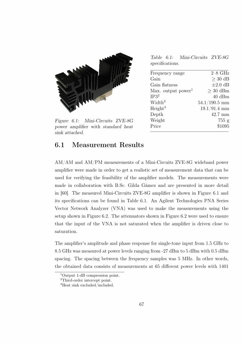
Figure 6.1: Mini-Circuits ZVE-8Gpower amplifier with standard heatsink attached.

Table 6.1: Mini-Circuits ZVE-8Gspecifications.

Frequency range 2–8 GHzGain ≥ 30 dBGain flatness ±2.0 dBMax. output power1 ≥ 30 dBmIP32 40 dBmWidth3 54.1/190.5 mmHeight3 19.1/91.4 mmDepth 42.7 mmWeight 755 gPrice $1095

6.1 Measurement Results

AM/AM and AM/PM measurements of a Mini-Circuits ZVE-8G wideband power

amplifier were made in order to get a realistic set of measurement data that can be

used for verifying the feasibility of the amplifier models. The measurements were

made in collaboration with B.Sc. Gilda Gámez and are presented in more detail

in [60]. The measured Mini-Circuits ZVE-8G amplifier is shown in Figure 6.1 and

its specifications can be found in Table 6.1. An Agilent Technologies PNA Series

Vector Network Analyzer (VNA) was used to make the measurements using the

setup shown in Figure 6.2. The attenuators shown in Figure 6.2 were used to ensure

that the input of the VNA is not saturated when the amplifier is driven close to

saturation.

The amplifier’s amplitude and phase response for single-tone input from 1.5 GHz to

8.5 GHz was measured at power levels ranging from -27 dBm to 5 dBm with 0.5 dBm

spacing. The spacing between the frequency samples was 5 MHz. In other words,

the obtained data consists of measurements at 65 different power levels with 1401

1Output 1-dB compression point.2Third-order intercept point.3Heat sink excluded/included.

67

Agilent Technologies E8363A PNA SeriesMicrowave vector network analyzer

Mini-Circuits ZVE-8GPower amplifier

3 dBAttenuator

20 dBAttenuator

Figure 6.2: Single-tone measurement setup for AM/AM and AM/PM measurements.

frequency samples at each power level. Thus, the measurements can be considered to

be comprehensive enough to model the characteristics of the amplifier for single-tone

inputs.

The measured amplitude and phase response of the amplifier is shown in Figure 6.3.

As can be seen from the figure, the specifications given by the manufacturer shown

in Table 6.1 are a bit too optimistic at least for this individual amplifier. The out-

put gain of the amplifier at the center frequency of the claimed operating frequency

band, i.e., at 5 GHz was only 28.2 dB and the 1-dB input compression point was

calculated to be 0 dBm corresponding to a maximum output power of 27.2 dBm

at 5 GHz. On the other hand, the claimed gain flatness was reached for the whole

operating frequency band with a maximum in-band peak-to-peak ripple of 3.6 dB.

Nevertheless, the measurements correspond to the specifications given by the man-

ufacturer quite well and hence there is no reason to doubt that they would contain

any significant errors.

The AM/AM characteristics are obtained from the measurement results shown in

Figure 6.3 by plotting the output power as a function of the input power. Similarly,

the AM/PM characteristics are obtained by plotting the output phase shift as a

68

2 3 4 5 6 7 820

25

30

35−27 dBm input power−4 dBm input power0 dBm input power5 dBm input power

← −27 dBm

← −4 dBm

← 0 dBm

5 dBm →

Frequency (GHz)

Gai

n(d

B)

(a) Amplitude response.

2 3 4 5 6 7 8−4000

−3500

−3000

−2500

−2000

−1500

−1000

−500

0

−27 dBm input power−4 dBm input power0 dBm input power5 dBm input power

Frequency (GHz)

Phas

e(d

eg.)

(b) Phase response

Figure 6.3: Measured amplitude and phase response of the Mini-Circuits ZVE-8Gpower amplifier at selected power levels. Attained gain at 5 GHz was 28.2 dB andthe 1-dB input compression point was 0 dBm. The maximum peak-to-peak ripplewas 3.6 dB within 2–8 GHz at 0 dBm input power.

69

function of the input power. The obtained AM/AM and AM/PM characteristics

at selected frequencies are shown in Figure 6.4. From the AM/AM characteristics

shown in Figure 6.4(a) it is easy to observe that the claimed 30 dBm maximum

output power was not reached. The AM/PM characteristics on the other hand

show that the phase distortion is within the typical 10 degree maximum phase shift

of SSPAs at the 1-dB compression point. Note that in order to make the evaluation

of the phase distortion at different frequencies easier, the phase characteristics in

Figure 6.4(b) are normalized to zero degree phase shift at the smallest measured

input power level (-27 dBm).

6.2 Least-Squares Estimation of the Polynomial

Model Coefficients

This section presents a least-squares solution for solving the coefficients of the poly-

nomials in Equation (4.1). An outline of the steps for finding the solution is as

follows. To present the solution in a clear and compact form, both the measurement

data and the polynomial model are first formulated in vector notation. After that,

the least-squares estimation problem for the vector parameter polynomial model is

formulated and its Least-Squares Estimator (LSE) is derived. Finally, some aspects

of how to improve the accuracy and efficiency of the estimation are presented as well

as conclusions of the efficiency of the derived LSE.

The obtained AM/AM and AM/PM measurement results at a given frequency can

be presented by three vectors

pin =[

pin(0) pin(1) · · · pin(L− 1)]T

(6.1a)

pout =[

pout(0) pout(1) · · · pout(L− 1)]T

(6.1b)

φout =[

φout(0) φout(1) · · · φout(L− 1)]T

(6.1c)

70

−25 −20 −15 −10 −5 0 50

5

10

15

20

25

30

2 GHz input tone4 GHz input tone6 GHz input tone8 GHz input tone

Input power (dBm)

Outp

ut

pow

er(d

Bm

)

(a) AM/AM characteristics.

−25 −20 −15 −10 −5 0 5−10

−5

0

5

10

15

20

2 GHz input tone4 GHz input tone6 GHz input tone8 GHz input tone

Input power (dBm)

Outp

ut

phas

esh

ift

(deg

.)

(b) AM/PM characteristics.

Figure 6.4: Measured amplitude and phase conversion characteristics of the Mini-Circuits ZVE-8G power amplifier at selected frequencies. The phase characteristicshave been normalized to yield a zero degree phase shift at -27 dBm in order to makethe evaluation of phase distortion at different frequencies easier.

71

where pin contains the input power values, pout contains the measured output power

values, φout contains the measured output phase shift values and L is the number

of measured frequency points. The polynomial model, on the other hand, can be

expressed in vector notation by defining the coefficient vectors a and b

a =[

a0 a1 · · · aN

]T

(6.2a)

b =[

b0 b1 · · · bN

]T

(6.2b)

and the observation matrix U

U =

1 pin(0) p2in(0) · · · pN

in(0)

1 pin(1) p2in(1) · · · pN

in(1)...

......

. . ....

1 pin(L− 1) p2in(L− 1) · · · pN

in(L− 1)

(6.3)

where U has the special form of a Vandermonde matrix [61]. Using Equations (6.1a),

(6.2) and (6.3), the polynomial model described by Equations (4.1a) and (4.1b) can

be expressed in vector notation as

g(pin) = Ua (6.4a)

Φ(pin) = Ub. (6.4b)

As can be seen from Equation (6.4), the polynomial model is linear in coefficients

and hence linear least-squares estimation that was presented in Chapter 3.6.1 can

be directly applied to solve it. Remembering that the LSE minimizes the squared

distance between the measured data and the estimated data, the estimation problem

can be written as

E(a) = (pout −Ua)T(pout −Ua) (6.5a)

E(b) = (φout −Ub)T(φout −Ub). (6.5b)

72

The LSE for the polynomial model in Equation (6.5) is defined in Equation (3.43)

and hence the LSEs of a and b are

a =(UTU

)−1UTpout (6.6a)

b =(UTU

)−1UTφout. (6.6b)

The accuracy of the estimators a and b is affected by two types of errors. First, ex-

perimental errors arise from the measurements since no instrument is able to provide

completely accurate measurements. Second, solving the estimators in Equation (6.6)

using a computer introduces roundoff errors. Naturally, it is desirable that these er-

rors affect the obtained estimator as little as possible. If small relative changes in

the data due to, e.g., roundoff errors cause small relative changes in the estimator,

the system is called well-conditioned ; otherwise the system is called ill-conditioned.

The inaccuracy of an estimator can be examined by the relative change defined as

∆(ξ) =‖ξ − ξ‖‖ξ‖ (6.7)

where ‖ · ‖ denotes the norm1, ξ is the original estimator and ξ is the estimator of

the modified system. Using the condition number defined as

cond(A) =

√

λmin

λmax

(6.8)

where λmin and λmax are the smallest and largest eigenvalues, respectively, of AHA,

then an upper bound for the relative change of the estimators in Equation (6.6) can

be written as [2]

∆(a) ≤ cond(UTU)∆(UTpout) (6.9a)

∆(b) ≤ cond(UTU)∆(UTφout). (6.9b)

1‖ξ‖2 = ξHξ where ξ is a vector in Cn and H denotes the Hermitian operation, i.e, transposition

with conjugation.

73

Equation (6.9) shows that if the condition number of UTU is small, then a small

relative change of UTpout and UTφout force a small relative change of a and b. On

the other hand, if the condition number of UTU is large then the relative change

of a and b might still be small, even if the relative change of UTpout and UTφout

is large. In short, a large condition number of UTU indicates possibility for large

relative errors.

In order to make sure that UTU is well-conditioned, its condition number can be

reduced by normalizing the input vector pin. This is especially important if the

order of the model is high which indicates that the spread of the eigenvalues of

UTU is large. In such a situation, improved estimates of a and b can be obtained

by centering pin to zero mean and scaling it to unit standard deviation

pin,normalized =pin −mean(pin)

std(pin). (6.10)

Further improvement of accuracy can be obtained by using weighted least-squares

estimation discussed in Chapter 3.6.2. The weighted least-squares estimation prob-

lem can be formulated as

E(a) = (pout −Ua)TWa(pout −Ua) (6.11a)

E(b) = (φout −Ub)TWb(φout −Ub). (6.11b)

where Wa and Wb are weighting matrices of the measured output power values

and the measured output phase shift values, respectively. The estimation problem

in Equation (6.11a) can be solved using Equation (3.46) and thus the Weighted

Least-Squares Estimators (WLSE) of a and b are

a =(UTWaU

)−1UTWapout (6.12a)

b =(UTWbU

)−1UTWbφout. (6.12b)

The WLSE can be used to improve the accuracy of the estimation by emphasizing

a desired power range. Furthermore, it can be used to improve the accuracy of

74

the estimation when some of the measured data values are less reliable than others.

Giving more weight to the more reliable values will give more accurate results.

As discussed in Chapter 3.6, the performance of neither the LSE nor the WLSE

can be guaranteed unless some assumptions can be made about the noise embedded

in the model. If the noise can be assumed to be white then the derived LSE for

the polynomial model is equivalent to the Minimum Variance Unbiased Estimator

(MVUE). On the other hand, if the noise is colored, then the weighting matrix of

the WLSE should be chosen as the inverse of the noise covariance matrix in order for

it to be the MVUE. Generally, the noise produced by the power amplifier and the

measurement equipment can be assumed Additive White Gaussian Noise (AWGN).

Therefore, the derived LSE is an optimal estimator for the polynomial model, in the

sense that it produces the MVUE.

6.3 Estimation Results

This section presents the estimation results obtained using the polynomial model.

The polynomial model was fitted to the 6 GHz AM/AM and AM/PM measurement

results shown in Figure 6.4 using the LSE stated in Equation (6.6). The result is

shown in Figure 6.5 where a fifth-order polynomial is fitted to both the AM/AM and

AM/PM conversion characteristics. Results similar to those shown in Figure 6.5 are

obtained for any given frequency.

In order to evaluate the accuracy of the AM/AM estimation, the relative Root-

Mean-Square (RMS) error was calculated. Using the error function defined in Equa-

tion (6.5a), the relative RMS error for the AM/AM estimation can be written as

ERMS,relative(a) = 10 lg

(‖pout −Ua‖‖pout‖

)

. (6.13)

The relative RMS error of the AM/AM estimation is plotted as a function of the

order of the polynomial in Figure 6.6(a). The AM/PM estimation accuracy was

75

−25 −20 −15 −10 −5 0 50

5

10

15

20

25

30

6 GHz input tone5th−order fit to 6 GHz tone

Input power (dBm)

Outp

ut

pow

er(d

Bm

)

(a) AM/AM estimation.

−25 −20 −15 −10 −5 0 5−10

−5

0

5

10

15

20

6 GHz input tone5th−order fit to 6 GHz tone

Input power (dBm)

Outp

ut

phas

esh

ift

(deg

.)

(b) AM/PM estimation.

Figure 6.5: A 5th-order least-squares polynomial fit of the measured AM/AM andthe AM/PM characteristics at 6 GHz. The relative RMS error of the AM/AMestimation is –18.18 dB and the RMS error of the AM/PM estimation is 0.19 degrees.

evaluated using the Root-Mean-Square error defined as

ERMS(b) =

∥∥∥φout −Ub

∥∥∥

√L

(6.14)

where L is the number of the measured frequency points. The RMS error describes

how much the estimated data values differ from the measured data values on the

average. The RMS error of the AM/PM estimation is plotted as function of the

order of the polynomial in Figure 6.6(b).

The relative RMS error of the fifth-order AM/AM estimation shown in Figure 6.5(a)

was −18.18 dB and the RMS error of AM/PM estimation shown in Figure 6.4(b)

was 0.19 degrees. Increasing the order of the polynomial from 5 to 11 reduces the

error of both the AM/AM and AM/PM estimation significantly but increasing the

order further does not yield substantial improvement of the estimation result as can

be seen from Figure 6.6.

Since the polynomial model is fitted to the measurements at a single frequency,

its capabilities to model AM/AM and AM/PM characteristics at other frequencies

76

5 10 15 20 25−30

−25

−20

−15

−10

−5

0

Order of the polynomial

Rel

ativ

eR

MS

erro

r(d

B)

(a) AM/AM estimation error.

5 10 15 20 250

0.1

0.2

0.3

0.4

0.5

0.6

0.7

0.8

0.9

1

Order of the polynomial

RM

Ser

ror

(deg

.)

(b) AM/PM estimation error.

Figure 6.6: Error of the estimated AM/AM conversion and the estimated AM/PMconversion at 6 GHz as a function of the order of the polynomial. The relative RMSerror of the AM/AM estimation plotted in (a) is defined in Equation (6.13) and theRMS error of the AM/PM estimation plotted in (b) is defined in Equation (6.14).

must be verified separately. This is illustrated in Figure 6.7 where the measured

AM/AM and AM/PM characteristics are compared to the estimated AM/AM and

AM/PM characteristics at selected frequencies. In the figure the estimation error of

two 5th-order polynomials are shown. The first polynomial is fitted to the measured

2 GHz AM/AM and AM/PM characteristics and the second polynomial is fitted to

the 6 GHz AM/AM and AM/PM characteristics.

Naturally the estimation error has a minimum at the estimated frequency, but it

is interesting to see how well the model estimates the AM/AM and AM/PM char-

acteristics of other frequencies. The polynomial fitted to the 2 GHz characteristics

models poorly the AM/AM and AM/PM characteristics of other frequencies, whilst

the polynomial fitted to the 6 GHz measurements can be considered quite accurate

between 5 GHz and 6.5 GHz.

The AM/AM characteristics estimation error behavior is an obvious consequence

of the amplifier’s amplitude response plotted in Figure 6.3(a), which shows that

the amplitude response has a peak at 2 GHz, but is almost flat around 6 GHz.

77

2 3 4 5 6 7 8−30

−25

−20

−15

−10

−5

0

5Polynomial fitted to 2 GHz measurementsPolynomial fitted to 6 GHz measurements

Frequency (GHz)

Rel

ativ

eR

MS

erro

r(d

B)

(a) AM/AM estimation error

2 3 4 5 6 7 80

1

2

3

4

5

6

7Polynomial fitted to 2 GHz measurementsPolynomial fitted to 6 GHz measurements

Frequency (GHz)

RM

Ser

ror

(deg

.)

(b) AM/PM estimation error

Figure 6.7: Difference between the measured AM/AM & AM/PM and the estimatedAM/AM & AM/PM characteristics of 5th-order polynomials fitted to selected fre-quencies. The relative RMS error of the AM/AM estimation plotted in (a) is definedin Equation (6.13) and the RMS error of the AM/PM estimation plotted in (b) isdefined in Equation (6.14).

The phase response has similar characteristics, but it is more difficult to observe it

from Figure 6.3(b) since the phase shift is very small compared to the group delay

of the amplifier. In order to use frequency-independent modelling techniques, the

frequency response of the amplifier should be constant on the desired frequency

band.

6.4 Summary

In this chapter the polynomial model discussed in Chapter 4.1 was applied for

frequency-independent estimation of a Mini-Circuits ZVE-8G power amplifier. First,

the measurement setup was introduced and the obtained measurement data were

presented. Next, the measurement data and the polynomial model were formulated

in vector notation and thereafter an optimal least-squares estimator was derived for

estimation of the coefficients of the polynomials. Finally the estimation results were

78

presented and the error behavior of the polynomial model was analyzed.

The estimation accuracy of the polynomial model for a single frequency is very

good even for models of low order. Accurate results were obtained using a fifth-

order polynomial model. The relative RMS error of the AM/AM estimation was

−18.18 dB and the RMS error of the AM/PM estimation was 0.19 degrees. The

estimation accuracy can be improved using a higher-order model, but increasing the

order above 11 does not yield substantial improvement of the estimation. The poly-

nomial model’s capability to estimate other frequencies than the fitting frequency

was also studied.

The AM/AM and AM/PM characteristics play a crucial role in this since the poly-

nomial is not able to model the frequency dependent behavior of the amplifier.

Quite good estimation performance can be obtained if the amplifier is designed to

have nearly flat gain and phase characteristics. However, if the amplifier is fed by

wideband signals and has non-flat characteristics, a frequency-dependent model is

required.

79

Chapter 7

Frequency-Dependent Estimation of

Power Amplifier Nonlinearity Using

the Hammerstein Model

The objective of this chapter is to model the measured frequency-dependent non-

linear behavior of the Mini-Circuits ZVE-8G power amplifier using a Hammerstein

model as discussed in Chapter 5.2. The estimation problem is to minimize the dif-

ference between the output of the power amplifier and the Hammerstein model as

illustrated in Figure 7.1.

The required measurements were discussed in Chapter 6.1 and the measured ampli-

tude and phase response of the Mini-Circuits ZVE-8G power amplifier were plotted

in Figures 6.3 and 6.4. A picture of the Mini-Circuits ZVE-8G power amplifier was

shown in Figure 6.1 and its specifications were presented in Table 6.1.

A brief outline of this chapter follows. First, the chosen implementation of the

Hammerstein model is discussed. As shown in Figure 7.1, the nonlinear static block

is implemented by the polynomial model discussed in Chapter 4.1 and the linear

dynamic block is implemented as an FIR filter. The following section presents a

80

ZVE-8GPower amplifier

Polynomial modelg(A), Φ(A)

FIR filterH(ω)

Nonlinear static block Linear dynamic block

-x e

Figure 7.1: Block diagram of the frequency-dependent estimation problem for theHammerstein model where x is the input that is fed to both the power amplifierand the model and e is the error of the estimation. The nonlinear static blockis implemented by the polynomial model discussed in Chapter 4.1 and the lineardynamic block is implemented as an FIR filter.

simple estimation method for determining the parameters of the two blocks sepa-

rately. After that a solution for estimating the coefficients of the FIR filter that

implements the linear dynamic block of the Hammerstein model is derived. Finally,

the estimation results of both the FIR design and the Hammerstein model are pre-

sented and the estimation error is analyzed. The chapter ends with a summary of

the obtained results.

7.1 Implementation of the Hammerstein Model

This section presents the implementation of the Hammerstein model for estimation

of the Mini-Circuits ZVE-8G power amplifier. As earlier mentioned in Chapter 5.2

the Hammerstein model is a cascade of a nonlinear static block and a linear dynamic

block. Typically the static nonlinearity is implemented as a polynomial and the

linear dynamic block as an IIR or an FIR filter [50].

Chapter 6 showed that the polynomial model can estimate the nonlinearity of the

amplifier quite well at a single frequency and therefore, it is chosen to implement

the nonlinear static block. For simplicity, an FIR filter was chosen to implement

81

the linear dynamic block. Besides simplicity of design and implementation, FIR

filters are also superior to IIR filters in that they are always stable, exhibit less

quantization noise when implemented in fixed-point arithmetic, and have smoother

phase characteristics [62].

7.2 Simplified Parameter Estimation of the

Hammerstein Model

This section defines the estimation problem for the Hammerstein model and proposes

a solution for separately determining the parameters of the two cascaded blocks.

The estimation problem for the chosen implementation of the Hammerstein model

is illustrated in Figure 7.1. The objective is to minimize the difference between the

output of the power amplifier and the output of the Hammerstein model based on

the measured frequency response.

The frequency response of the Mini-Circuits ZVE-8G power amplifier that was plot-

ted in Figure 6.3 clearly shows that both the amplitude and phase response of the

power amplifier depend on the input power level. Therefore the explicit estimation

problem is to minimize the difference between the desired complex-valued power-

dependent frequency response Hd,p(Al, ωk) and the estimated complex-valued power-

dependent frequency response Hp(Al, ωk). Mathematically this can be formulated

as

E =∣∣Hd,p(Al, ωk)−Hp(Al, ωk)

∣∣2

(7.1)

where Al and ωk are the discrete amplitude and frequency points at which both

Hd,p and Hp are evaluated. Direct minimization of the error function defined in

Equation (7.1) is very difficult and hence the estimation problem must be further

simplified. Note that the error measure in Equation (7.1) is chosen so that the

required measurements can be done with the available equipment.

82

Denoting the frequency response of the FIR filter as H(ωk), the estimated power-

dependent frequency response Hp(Al, ωk) can be written as

∣∣Hp(Al, ωk)

∣∣ = g(Al)

∣∣H(ωk)

∣∣ (7.2)

∠Hp(Al, ωk) = Φ(Al) + ∠H(ωk) (7.3)

where g(Al) is the AM/AM, and Φ(Al) is the AM/PM conversion function of the

polynomial model. Using Equations (7.2) and (7.3) the estimation problem defined

by the error function in Equation (7.1) can be rewritten as two separate estimation

problems where the objective is to minimize the error functions

Eg =∣∣∣

∣∣Hd,p(Al, ωk)

∣∣− g(Al)

∣∣H(ωk)

∣∣

∣∣∣

2

(7.4a)

EΦ =∣∣∣∠Hd,p(Al, ωk)− Φ(Al)− ∠H(ωk)

∣∣∣

2

(7.4b)

where Eg is the error function for the amplitude response estimation problem and

EΦ is the error function for the phase response estimation problem.

A simplified solution for the estimation problem defined by the error functions in

Equation (7.4) can be found in [63] where g(Al), Φ(Al), |H(ωk)| and ∠H(ωk) are

approximated by polynomials. Unfortunately, the presented solution has some draw-

backs and the authors only recommend it as a starting point for estimation of Ham-

merstein systems. First, the conversion of the nonlinear estimation problem into a

linear estimation problem causes some excess error to the solution. Second, the so-

lution is quite complex even though only linear estimation methods are used. Third,

the FIR filter is merely described by the polynomials approximating the amplitude

and phase response instead of being identified by its coefficients.

In the following a simplified estimation problem is formulated for determining the

coefficients of both the polynomial model and the FIR filter of the Hammerstein

model shown in Figure 7.1. The estimation problem defined by the error function

in Equation (7.1) is simplified by assuming that the identification of the two blocks

can be done separately. The static nonlinearity is assumed to be given by the

83

AM/AM and AM/PM measurements at the center frequency of the desired operating

band. The linear dynamic part is assumed to be given by the small-signal frequency

response of the modelled system. Mathematically, the estimation problem is to

minimize the error functions

Eg =∣∣Ad,l − g(Al)

∣∣2

(7.5a)

EΦ =∣∣φds,l − Φ(Al)

∣∣2

(7.5b)

EH =∣∣Hd,s0

(ωk)−H(ωk)∣∣2

(7.5c)

where Ad,l are the desired discrete output amplitude values, φds,l are the desired

scaled discrete output phase values and Hd,s0(ωk) is the desired scaled discrete small-

signal response. The desired discrete output phase values must be scaled to zero

degree at the small-signal input power level As at which H(ωk) is fitted to or else the

phase delay of the amplifier is included twice in the estimation. Similarly, the small-

signal response Hd,s(ωk) must be scaled to have unit gain at the center frequency

ωc at which g(A) and Φ(A) are fitted to. Otherwise the gain of the amplifier is

included twice in the estimation. Mathematically the required scaling operations

can be written as

φds,l = φd,l − φd,s (7.6)

∣∣Hd,s0

(ωk)∣∣ =

∣∣Hd,s(ωk)

∣∣

|Hd,s(ω0)|. (7.7)

The estimation problem (minimization of the error functions in Equation (7.5))

can be solved in three steps. First, the output phase values φd,l and the small-

signal frequency response Hd,s(ω) are scaled as described by Equations (7.6) and

(7.7) to obtain φds,l and Hd,s0(ω). Second, the coefficients of the polynomial model

are estimated using the least-squares solution that was presented in Chapter 6.2.

Finally, the coefficients of the FIR filter are estimated using weighted least-squares

estimation that will be presented in Chapter 7.3. The proposed estimation technique

is summarized in Table 7.1.

84

Table 7.1: Proposed technique for simplified parameter estimation of the Hammer-stein model. The objective is to find the coefficients of the gain distortion functiong(Al), the phase distortion function Φ(Al) and the FIR filter H(ω).

Required input data

Al A set of L discrete input amplitude valuesAs Input amplitude level of the measured small-signal frequency responseωk A set of K discrete angular frequencies contained in [−π, π]ωc Center frequency of the desired frequency band

Required output data

Ad,l The desired discrete output amplitude values at ωc

φd,l The desired discrete output phase values at ωc

Hd,s(ωk) The desired discrete complex-valued frequency response at As

Problem formulation

The estimation problem is to choose the coefficients of g(Al), Φ(Al)and H(ωk) so that the least-squares error functions are minimized:

Eg =∣∣Ad,l − g(Al)

∣∣2

EΦ =∣∣φds,l − Φ(Al)

∣∣2

EH =∣∣Hd,s0

(ωk)−H(ωk)∣∣2

Solution

Step 1: Determine φds,l and Hd,s0(ωk) by scaling φd,l and Hd,s(ωk)

φds,l = φd,l − φd,s

|Hd,s0(ωk)| = |Hd,s(ωk)| / |Hd,s(ω0)|

Step 2: Estimate coefficients of g(Al) and Φ(Al) using the least-squares solutionpresented in Chapter 6.2

Step 3: Estimate coefficients of Hd,s0(ωk) using the weighted least-squares so-

lution presented in Chapter 7.3

85

The justification for this simplified estimation technique is that in a moderate to

large-backoff condition the modelled amplifier performs almost linearly and the

small-signal transfer function is what the signal can be expected to see. In saturated

operation the signal can instead be expected to see the saturated transfer function.

The difference between the estimation technique proposed here and the estimation

technique defined by the error function in Equation (7.4) is that here the estimation

of the blocks is assumed separable instead of assuming that the estimation of the

amplitude and phase characteristics are separable.

It should be noted that the FIR filter is a baseband approximation of the measured

frequency response. This means that the required sampling rate easily becomes very

high. According to the sampling theorem1, a bandlimited signal contained in [f1, f2]

can be uniquely determined by its samples, if and only if the sampling frequency

fs satisfies fs > 2f2 [64]. The highest frequency f2 is usually called the Nyquist

frequency since it determines the minimum sampling frequency fs = 2f2 called the

Nyquist rate. The Nyquist rate for baseband FIR approximation is illustrated in

Figure 7.2(a).

In practice only a relatively small subband of the whole frequency range of the

amplifier is interesting. In such a case the sampling rate can be significantly reduced

by first bandpass filtering the desired subband and then demodulating the filtered

subband to baseband. An illustration of the filtering and demodulation process is

shown in Figure 7.2. As an example let us consider that we are only interested in

modelling the frequency band from 5 GHz to 7 Ghz, i.e., we have f1 = 1.5 Ghz, f2 =

8.5 GHz, fd,1 = 5 GHz and fd,2 = 7 GHz in Figure 7.2(a). Baseband approximation

of the desired band requires a minimum sampling rate fs,1 = 17 GHz, since the

Nyquist frequency is 8.5 GHz (see Fig. 7.2(a)). On the other hand, the Nyquist

rate for the filtered and demodulated band is only fs,2 = 2 GHz, since we now have

fd0,1 = −1 GHz and fd0,2 = 1 GHz (see Fig. 7.2(b)).

1Also called either the Nyquist sampling theorem or the Shannon sampling theorem.

86

0 f1 fd,1 fd,2 f2 fs,1-f1-fd,1-fd,2-f2-fs,1

(a)

0fd0,1 fd0,2 fs,1fs,2-fs,1 -fs,2

(b)

Figure 7.2: Illustration of the minimum sampling rate for the FIR filter design.(a) Baseband approximation of the signal contained in the range [f1, f2], where theminimum sampling rate is fs,1 = f2. (b) Desired subband contained in the range[fd0,1, fd0,2] after bandpass filtering and demodulation to baseband. The requiredsampling rate is now only fs,2 = fd0,2.

7.3 Weighted Least-Squares FIR Approximation

Weighted least-squares approximation can be used to design FIR filters with desired

arbitrary shape amplitude and phase response [62]. A solution for the continuous

frequency case can be found in [65]. In this chapter the derivation presented in [65]

is modified for use on a discrete frequency grid.

The frequency response of a Mth-order (M + 1 coefficients) causal FIR filter is

defined as

H(ejωk

)=

M∑

m=0

hme−jωkm (7.8)

where the filter coefficients h0, h1, . . . , hm are assumed to be real valued and ωk is

a set of discrete angular frequencies where the response is evaluated. The com-

putational complexity of the filter described by Equation (7.8) can be reduced by

adding a delay element with a constant delay of D samples before the filter. This

is equivalent to setting the first D coefficients of the filter to zeroes. The frequency

87

h0 h1 h2 hM−1 hM

z−Dx(k)

y(k)

z−1z−1 z−1

Figure 7.3: A Direct Form I realization of a causal Mth-order FIR filter. The FIRfilter is preceded by a delay element with a constant delay of D samples.

response of the cascade of the delay element and the FIR filter is

H(ejωk

)=

M∑

m=0

hme−jωk(m+D). (7.9)

An implementation of the system described by Equation (7.9) is shown in Figure 7.3

where the FIR filter has been realized using the Direct Form I structure [51].

The filter design problem is to choose the filter coefficients h0, h1, . . . , hM so that

the weighted least-squares error is minimized:

E =K−1∑

k=0

W (ωk)

∣∣∣∣∣Hd

(ejωk

)−

M∑

m=0

hme−jωk(m+D)

∣∣∣∣∣

2

(7.10)

where ωk is a set of K discrete angular frequencies in the range [−π, π], Hd (ejωk) is

the desired complex-valued frequency response, W (ωk) is a real-valued nonnegative

weight function, M is the desired order of the filter and D is the desired length of

the constant delay element.

In order for the design problem described by Equation (7.10) to have a solution it

is required that K ≥ M . Obviously, the error is only minimized at the K sample

points and hence a small enough frequency grid should be used in order to make

the frequency response of the filter well behaved between the sample points. In

other words, a large ratio of K/M indicates a more constrained error between the

sample points. On the other hand choosing K > M results in more equations than

88

unknowns and hence only approximate solutions are possible.

For K = M the design problem can also be solved using the frequency sampling

technique in which the filter coefficients are directly calculated from the desired fre-

quency response using the Inverse Discrete Fourier Transform (IDFT). Naturally the

use of IDFT requires that the sample points are equally spaced. Another drawback

of the frequency sampling technique is that the frequency response is unconstrained

between the sample points which might lead to large errors between the sample

points if the desired phase response is in some way inconsistent with the amplitude

response or the filter length [62]. Due to the possibility of large errors in the fre-

quency response, the frequency sampling technique is not useful for the Hammerstein

model.

To present the solution of Equation (7.10) in a clear and compact form, the problem

is first rewritten in vector notation. Denoting the real-valued filter coefficient vector

h and the complex-valued discrete-time Fourier transform vector e as

h =[

h0 h1 · · · hM

]T

(7.11)

e (ωk) =[

e−jωkD e−jωk(D+1) · · · e−jωk(D+M)]T

(7.12)

the error function defined in Equation (7.10) can be rewritten in vector notation as

E =K−1∑

k=0

W (ωk)∣∣Hd

(ejωk

)− hTe (ωk)

∣∣2. (7.13)

Equation (7.13) can be written more compactly as (see Appendix A for details)

E = hTPh− 2hTp1 + p0 (7.14)

89

where

P =K−1∑

k=0

W (ωk)C (ωk) (7.15)

p1 =K−1∑

k=0

W (ωk)

[

Re

Hd

(ejωk

)

c (ωk)− Im

Hd

(ejωk

)

s (ωk)

]

(7.16)

p0 =K−1∑

k=0

W (ωk)∣∣Hd

(ejωk

)∣∣2

(7.17)

and

c (ωk) =[

cos Dωk cos(D + 1)ωk · · · cos(D + M)ωk

]T

(7.18)

s (ωk) =[

sin Dωk sin(D + 1)ωk · · · sin(D + M)ωk

]T

(7.19)

C (ωk) =

1 cos (ωk) · · · cos (Mωk)

cos (ωk) 1 · · · cos [(M − 1) ωk]...

.... . .

...

cos (Mωk) cos [(M − 1) ωk] · · · 1

. (7.20)

The solution to Equation (7.14) (see Appendix A for details) is given by

h = P−1p1. (7.21)

A Matlab implementation of the proposed design technique can be found in Ap-

pendix B. The computational complexity can be reduced by utilizing the Toeplitz

structure of P. The Levinson algorithm requires 4M2 floating-point operations to

solve the problem [61].

90

7.4 Estimation Results

This section presents the estimation results obtained using the Hammerstein model.

It seems justified to assume that in practice an amplifier is fed by signals that have a

relatively large bandwidth, but that the bandwidth is still considerably smaller than

the bandwidth of the amplifier. Therefore, it is reasonable to choose a subband of

the amplifier’s operating band and try to make the estimation as accurate as possible

on the chosen subband.

As earlier mentioned in Section 7.1, the static nonlinearity is implemented using the

polynomial model discussed in Chapter 4.1 and the linear dynamic system as an FIR

filter. The estimation results obtained using the polynomial model were presented

in Chapter 6.3. As can be seen from Figure 6.7, a 5th-order polynomial model fitted

to the 6 GHz measurements estimates the characteristics of the amplifier quite well

between 5 GHz and 7 GHz. Therefore, it is reasonable to choose the frequency band

from 5 GHz and 7 GHz as the desired estimation range.

A brief outline of this section follows. First, the weighted least-squares FIR approx-

imation discussed in Section 7.3 is verified by Matlab simulations. The following

subsection presents the FIR approximation of the measured small-signal response of

the Mini-Circuit ZVE-8G power amplifier. Finally, the estimation results using the

Hammerstein model are presented.

7.4.1 Verification of the Weighted Least-Squares FIR

Approximation

Before trying to estimate the small-signal frequency-response of the Mini-Circuits

ZVE-8G power amplifier, the weighted least-squares FIR approximation presented

in Section 7.3 is first verified by approximating a 5th-order lowpass Butterworth

filter. The cutoff frequency of the filter was set to fs/4 where fs is the sampling

frequency. Butterworth filters are of IIR-type and are characterized by a magnitude

91

0 0.1 0.2 0.3 0.4 0.5 0.6 0.7 0.8 0.9 1−50

−40

−30

−20

−10

0

10Desired response5th−order approximation7th−order approximation11th−order approximation

Normalized frequency

Am

plitu

de

(dB

)

(a) Amplitude response

0 0.1 0.2 0.3 0.4 0.5 0.6 0.7 0.8 0.9 1−900

−800

−700

−600

−500

−400

−300

−200

−100

0Desired response5th−order approximation7th−order approximation11th−order approximation

Normalized frequency

Phas

e(d

eg)

(b) Phase response

Figure 7.4: Frequency response of FIR filters designed using weighted least-squaresFIR approximation. The desired response of the FIR filters is a fifth-order lowpassButterworth filter with cutoff frequency fs/4 (normalized frequency 0.5).

response that is maximally flat in the passband and monotonic overall [62]. It should

be noted that Butterworth filters do not have linear phase response.

Using the frequency response of the Butterworth filter as the desired response, FIR

filters of selected orders were designed using the weighted least-squares FIR approx-

imation presented in Section 7.3. The obtained estimations of the desired frequency

response are shown in Figure 7.4. As can be seen from Figure 7.4(a), the FIR ap-

proximations are not flat in the passband as the desired response and the attained

stopband attenuation is significantly smaller. Nevertheless, the passband approxi-

mation is quite good and an 11th-order FIR filter can be considered to approximate

the desired amplitude response quite well.

The obtained estimates of the phase response are plotted in Figure 7.4(b). As in

the amplitude estimation, the passband approximation is again much better than

the stopband approximation. The high ripple of the desired response at half the

sampling frequency is caused by numerical problems since the values of the complex

frequency response approach the working precision of the computer. Generally, the

FIR approximation can be considered accurate and to produce filters with good

characteristics as can be seen from Figure 7.5. The pole-zero plot of the 11th-order

92

−1 −0.5 0 0.5 1

−1

−0.8

−0.6

−0.4

−0.2

0

0.2

0.4

0.6

0.8

1

Real part

Imag

inar

ypar

t

(a) Pole-zero plot

0 2 4 6 8 10 12 14 16 18

−0.5

−0.4

−0.3

−0.2

−0.1

0

0.1

0.2

0.3

0.4

0.5

Sample index

Am

plitu

de

(b) Impulse response

Figure 7.5: Illustration of the filter characteristics obtained using weighted least-squares FIR approximation. (a) Pole-zero plot and (b) impulse response of the11th-order FIR approximation of the desired 5th-order Butterworth filter response.

approximation plotted in Figure 7.5(a) shows that the designed filter has minimum-

phase2 characteristics which indicates that the filter has a small phase delay.

Obviously it is not possible to find an FIR filter that has exactly the same response

as an IIR filter. However, the approximation error should approach zero as the

order of the filter approaches infinity. Figure 7.6 shows that derived weighted least-

squares design technique fulfils this requirement. As can be seen from Figure 7.6,

the estimation error is decreasing monotonously until the working precision of the

computer is reached.

7.4.2 Results of the FIR Approximation

The accuracy of the weighted least-squares FIR approximation discussed in Sec-

tion 7.3 is affected by two factors. The principal factor is the order M of the FIR

filter. Increasing the order of the filter improves the estimation accuracy, however,

the computational complexity and the processing delay of the filter is increased. The

2A causal stable filter that has all its zeros and poles inside or on the unit circle is called aminimum-phase filter.

93

20 40 60 80 100 120 140−300

−250

−200

−150

−100

−50

0

Filter Order

Rel

ativ

eLS

Err

or(d

B)

Figure 7.6: Relative least-squares error of the weighted least-squares FIR approxi-mation as a function of the filter order. The desired response is a fifth-order lowpassButterworth filter with cutoff frequency fs/4.

computational complexity can be reduced by adding a delay element with a con-

stant delay D before the filter. This is equivalent to setting the first D coefficients

of the filter to zero. In other words, the delay element estimates the natural delay

of the modelled system. The second factor that affects the estimation accuracy is

the weight function W (ωk) that can be used to emphasize a desired subband of the

modelled system.

The simplest approach is to use a rectangular weighting function defined as

W (ωk) =

Wdesired, ωd,min ≤ ωk ≤ ωd,max

Wother, otherwise(7.22)

where Wdesired and Wother are constants (obviously Wother < Wdesired), ωd,min is the

lower bound and ωd,max is the upper bound of the desired band. The rectangular

weight function is described by the weighting factor Wf defined as

Wf =Wdesired

Wother

. (7.23)

A higher weighting factor yields more accurate results within the desired frequency

band. On the other hand, a small weighting factor constrains the error outside the

94

desired band more. Therefore, the weighting factor should be chosen small enough

to make the filter response well behaved while still being accurate.

As stated in Table 7.1, the FIR filter that implements the linear dynamic block of

the Hammerstein model should be designed to have equal response as the scaled

small-signal response of the modelled power amplifier. Figure 7.7 shows different

order approximations of the scaled small-signal response of the Mini-Circuits ZVE-

8G power amplifier. The length of the constant delay of each filter is chosen so that

the estimation error is minimized. All filters have been weighted using a rectangular

weight function with a weighting factor of 103.

As can be seen from Figure 7.7(a), a 7th-order filter is not yet able to completely

model the response, an 8th-order filter already performs quite well and increasing

the order above 13 does not significantly improve the estimation accuracy within

the desired frequency band due to the noise in the measurement data. Nevertheless

a higher-order filter results in a more well-behaved error outside the desired band.

Figure 7.7(b) shows that the phase estimation is less sensitive to the order of the

filter since the phase response is almost linear and good accuracy within the desired

band is obtained with all filters.

The effect of the weighting factor Wf is studied in Figure 7.8. The figure shows a

13th-order filter with a 17 sample constant delay fitted to the measured frequency

response with weighting factors 10, 103, 105 and 107. As can be seen from Fig-

ure 7.8(a), choosing the weighting factor as 10 results in too much ripple within the

desired frequency band. On the other hand, using a weighting factor of 107, the

error outside the desired band grows too high. In this case, choosing the weighting

factor between 103 and 105 gives good performance. Again, the phase estimation is

not as sensitive to the weighting factor as the amplitude estimation (see Fig. 7.8(b)).

95

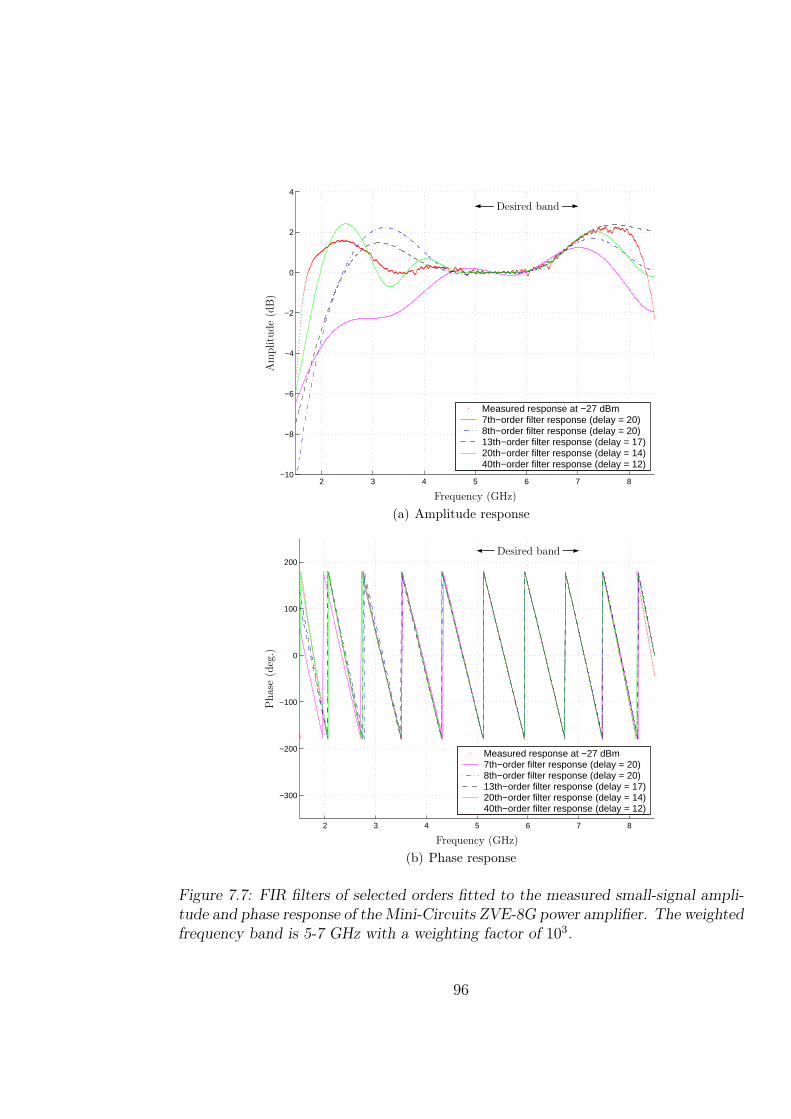
2 3 4 5 6 7 8−10

−8

−6

−4

−2

0

2

4

Measured response at −27 dBm7th−order filter response (delay = 20)8th−order filter response (delay = 20)13th−order filter response (delay = 17)20th−order filter response (delay = 14)40th−order filter response (delay = 12)

Desired band

Frequency (GHz)

Am

plitu

de

(dB

)


2 3 4 5 6 7 8

−300

−200

−100

0

100

200

Measured response at −27 dBm7th−order filter response (delay = 20)8th−order filter response (delay = 20)13th−order filter response (delay = 17)20th−order filter response (delay = 14)40th−order filter response (delay = 12)

Desired band

Frequency (GHz)

Phas

e(d

eg.)

(b) Phase response

Figure 7.7: FIR filters of selected orders fitted to the measured small-signal ampli-tude and phase response of the Mini-Circuits ZVE-8G power amplifier. The weightedfrequency band is 5-7 GHz with a weighting factor of 103.

96

2 3 4 5 6 7 8−10

−8

−6

−4

−2

0

2

4

Measured response at −27 dBmWeighting factor 10Weighting factor 103

Weighting factor 105


Desired band

Frequency (GHz)

Am

plitu

de

(dB

)


2 3 4 5 6 7 8

−300

−200

−100

0

100

200

Measured response at −27 dBmWeighting factor 10Weighting factor 103



Desired band

Frequency (GHz)

Phas

e(d

eg.)

(b) Phase response

Figure 7.8: Illustration of the effect of the weighting factor on the estimation ac-curacy. The order of the filter is 13 and the length of the constant delay is 17samples.

97

5 10 15 20 25 30 35 40 45 50 55 60

−40

−35

−30

−25

−20

−15

−10

−5

0 Weighting factor 10Weighting factor 103



Filter order

Rel

ativ

eLS

erro

ron

the

des

ired

ban

d(d

B)

(a)

0 5 10 15 20 25 30

−40

−35

−30

−25

−20

−15

−10

−5

0

7th−order filter8th−order filter13th−order filter20th−order filter40th−order filter

Delay

Rel

ativ

eLS

erro

ron

the

des

ired

ban

d(d

B)

(b)

Figure 7.9: Estimation accuracy of the weighted least-squares FIR approximation.(a) Effect of the filter order on the estimation accuracy for selected weighting factors.The length of the constant delay is zero samples. (b) Effect of the length of theconstant delay on the estimation accuracy for selected filter orders with a weightingfactor of 103.

The estimation accuracy is evaluated using the relative least-squares error defined

as

ELS,relative = 20 lg‖Hd (ωk)−H (ωk)‖

‖Hd (ωk)‖(7.24)

where Hd (ωk) is the desired complex-valued frequency response and H (ωk) is the

complex-valued frequency response of the designed filter. The effect of the filter

order on the estimation accuracy is shown in Figure 7.9(a) where the relative least-

squares error on the desired band is plotted as a function of the filter order. In order

to make the results comparable, the constant delay element was omitted. It should

be noted that the error is not monotonically decreasing, since only the error of the

desired band is considered. Figure 7.9(a) shows that increasing the order above

20 does not improve the estimation significantly if the weighting factor is chosen

properly. Using a weighting factor of 10 requires a very high-order filter in order

to produce accurate results. Sufficiently good estimation is obtained by choosing a

weighting factor of 103, and increasing it above 105 gives very little improvement in

the accuracy.

98

PSfrag replacemen

5th-orderpolynomial model 17 sample delay 13th-order FIRx y

Figure 7.10: Implementation of the Hammerstein model.

Figure 7.9(b) shows the relative least-squares error on the desired band as a func-

tion of the delay. Clearly, the filter order can be significantly reduced by using a

constant delay before the filter. This lowers the computational complexity of the

filter. However, it comes with the cost of a higher processing delay, since the delay

of the constant delay and the filter is greater than the delay of a higher-order filter

without a constant delay for a given error level. The figure also shows that delay

should be chosen carefully, since a too long delay increases the error rapidly.

7.4.3 Results of the Hammerstein Model Estimation

Now that the estimation results of both the polynomial model and the filter design

have been presented, the estimation results of the Hammerstein model can be pre-

sented. The nonlinear static block is implemented as 5th-order polynomial model

and the linear dynamic block as a 13th-order FIR filter with a constant delay of 17

samples and a weighting factor of 103. Figure 7.10 illustrates the chosen implemen-

tation of the Hammerstein model.

Figure 7.11 shows the estimated amplitude response at the boundaries of the dy-

namic range of the amplifier, i.e. at both –27 dBm and 0 dBm. As can be seen from

Figure 7.11(b), the estimation is very accurate within the desired frequency band

at both power levels. Improving the accuracy further is difficult due to the noise

in the measurement data. The estimated phase response is shown in Figure 7.12 at

power levels –27 dBm and 0 dBm. The figure shows that the phase estimation is

even better than the amplitude estimation on the desired band.

99

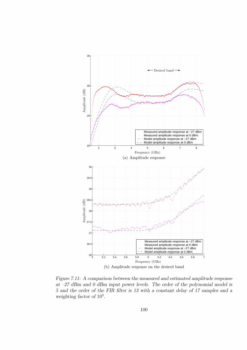
2 3 4 5 6 7 820

25

30

35

Measured amplitude response at −27 dBmMeasured amplitude response at 0 dBmModel amplitude response at −27 dBmModel amplitude response at 0 dBm

Desired band

Frequency (GHz)

Am

plitu

de

(dB

)


5 5.2 5.4 5.6 5.8 6 6.2 6.4 6.6 6.8 726

26.5

27

27.5

28

28.5

29

29.5

30

Measured amplitude response at −27 dBmMeasured amplitude response at 0 dBmModel amplitude response at −27 dBmModel amplitude response at 0 dBm

Frequency (GHz)

Am

plitu

de

(dB

)

(b) Amplitude response on the desired band

Figure 7.11: A comparison between the measured and estimated amplitude responseat –27 dBm and 0 dBm input power levels. The order of the polynomial model is5 and the order of the FIR filter is 13 with a constant delay of 17 samples and aweighting factor of 103.

100

2 3 4 5 6 7 8

−250

−200

−150

−100

−50

0

50

100

150

200

Measured phase response at −27 dBmMeasured phase response at 0 dBmModel phase response at −27 dBmModel phase response at 0 dBm

Desired band

Frequency (GHz)

Phas

e(d

eg.)

(a) AM/AM characteristics

5 5.2 5.4 5.6 5.8 6 6.2 6.4 6.6 6.8 7

−250

−200

−150

−100

−50

0

50

100

150

200

Measured phase response at −27 dBmMeasured phase response at 0 dBmModel phase response at −27 dBmModel phase response at 0 dBm

Frequency (GHz)

Phas

e(d

eg.)

(b) AM/AM characteristics at selected frequencies on the desired band

Figure 7.12: A comparison between the measured and estimated phase response at–27 dBm and 0 dBm input power levels. The order of the polynomial model is 5 andthe order of the FIR filter is 13 with a constant delay of 17 samples and a weightingfactor of 103.

101

The estimated AM/AM characteristics at selected frequencies on the operating band

of the amplifier are shown in Figure 7.13(a). The poor estimation result at 2 and 8

GHz is a consequence of the amplitude response of the FIR filter as can be seen from

Figure 7.11(a). However, the estimation result is very good on the desired band as

shown in Figure 7.13(b). Only the 7 GHz estimation is somewhat inaccurate at the

power range from 0 to 5 dBm, which is not very crucial since the 1-dB compression

point of the amplifier is at 0 dBm and hence it is not likely that the amplifier will

be used at such high input power levels.

Figure 7.14(a) shows the estimated AM/PM characteristics at selected frequencies

on the operating band. The figure shows that the estimation error outside the

desired band is approximately 5 to 10 degrees. Again the estimation result on the

desired band is very good as can be seen from Figure 7.14(b). The estimation seems

to be equally good on the whole desired band.

The estimation error of the Hammerstein model was defined in Equation (7.1) as

E =∣∣Hd,p(Al, ωk)−Hp(Al, ωk)

∣∣2

where Hd,p(Al, ωk) is the desired power-dependent frequency response and Hp(Al, ωk)

is the power-dependent frequency response of the model. The relative least-squares

error of the Hammerstein model can be written as

EA,ω(Al, ωk) = 20 lg

(∣∣Hd,p(Al, ωk)−Hp(Al, ωk)

∣∣2

∣∣Hd,p(Al, ωk)

∣∣2

)

. (7.25)

The error surface generated by Equation (7.25) is plotted in Figure 7.15(a) where

the desired band can be seen as a deep valley. Figure 7.15(b) shows the error surface

directly from above. From this figure it can be seen that the estimation is equally

good on the desired band for all power levels up to the 1-dB compression point.

102

−25 −20 −15 −10 −5 0 5

0

5

10

15

20

25

30

Measured characteristics at 2 GHzMeasured characteristics at 4 GHzMeasured characteristics at 6 GHzMeasured characteristics at 8 GHzEstimated characteristics at 2 GHzEstimated characteristics at 4 GHzEstimated characteristics at 6 GHzEstimated characteristics at 8 GHz

Input power (dBm)

Outp

ut

pow

er(d

Bm

)

(a) AM/AM characteristics

−25 −20 −15 −10 −5 0 5

0

5

10

15

20

25

30

Measured characteristics at 5 GHzMeasured characteristics at 5.5 GHzMeasured characteristics at 6 GHzMeasured characteristics at 6.5 GHzMeasured characteristics at 7 GHzEstimated characteristics at 5 GHzEstimated characteristics at 5.5 GHzEstimated characteristics at 6 GHzEstimated characteristics at 6.5 GHzEstimated characteristics at 7 GHz

Input power (dBm)

Outp

ut

pow

er(d

Bm

)

(b) AM/AM characteristics at selected frequencies on the desired band

Figure 7.13: A comparison between the measured and estimated AM/AM charac-teristics at selected frequencies. The order of the polynomial model is 5 and theorder of the FIR filter is 13 with a constant delay of 17 samples and a weightingfactor of 103.

103

−25 −20 −15 −10 −5 0 5

−350

−300

−250

−200

−150

−100

−50

0

50

100

150

200

Measured characteristics at 2 GHzMeasured characteristics at 4 GHzMeasured characteristics at 6 GHzMeasured characteristics at 8 GHzEstimated characteristics at 2 GHzEstimated characteristics at 4 GHzEstimated characteristics at 6 GHzEstimated characteristics at 8 GHz

Input power (dBm)

Outp

ut

phas

e(d

eg.)

(a) AM/PM characteristics

−25 −20 −15 −10 −5 0 5

−350

−300

−250

−200

−150

−100

−50

0

50

100

150

200

Measured characteristics at 5 GHzMeasured characteristics at 5.5 GHzMeasured characteristics at 6 GHzMeasured characteristics at 6.5 GHzMeasured characteristics at 7 GHzEstimated characteristics at 5 GHzEstimated characteristics at 5.5 GHzEstimated characteristics at 6 GHzEstimated characteristics at 6.5 GHzEstimated characteristics at 7 GHz

Input power (dBm)

Outp

ut

phas

e(d

eg.)

(b) AM/PM characteristics at selected frequencies on the desired band

Figure 7.14: A comparison between the measured and estimated AM/PM charac-teristics at selected frequencies. The order of the polynomial model is 5 and theorder of the FIR filter is 13 with a constant delay of 17 samples and a weightingfactor of 103.

104

The estimation error is further analyzed by calculating the average relative least-

squares error for a given frequency

Eω(ωk) = 20 lg

L−1∑

l=0

∣∣∣Hd,p(Al, ωk)−Hp(Al, ωk)

∣∣∣

2

L−1∑

l=0

∣∣∣Hd,p(Al, ωk)

∣∣∣

2

(7.26)

and the average relative least-squares error for a given input power level

EA(Al) = 20 lg

K−1∑

k=0

∣∣∣Hd,p(Al, ωk)−Hp(Al, ωk)

∣∣∣

2

K−1∑

k=0

∣∣∣Hd,p(Al, ωk)

∣∣∣

2

. (7.27)

The error measures defined by Equations (7.26) and (7.27) are plotted in Fig-

ures 7.15(c) and 7.15(d) respectively. Figure 7.15(c) can be thought of as a cross-

section of Figure 7.15(a) at a given input power level. In the figure the estimation

error has been averaged over all power levels, and for power levels up to the 1-dB

compression point. There is almost no difference in the curves since all power levels

are equally weighted. The figure shows that the estimation accuracy is very good

on the desired band and that the estimation error is constrained outside the desired

band. Therefore the estimation results can be considered very good.

Similarly, Figure 7.15(d) can be thought of as a cross-section of Figure 7.15(a) at

a given frequency. This figure shows that estimation accuracy is almost constant

at power levels up to the 1-dB compression point. At higher input power levels

the nonlinearity of the power amplifier increases which naturally implies reduced

estimation accuracy. This is not crucial since it is not likely that the amplifier will

be driven at input power levels above the 1-dB compression point.

105

(a) (b)

2 3 4 5 6 7 8−100

−80

−60

−40

−20

0

20Error averaged over input power levels between −27 dBm and 5 dBmError averaged over input power levels between −27 dBm and 0 dBm

Frequency (GHz)

Rel

ativ

eLS

erro

r(d

B)

(c)

−25 −20 −15 −10 −5 0 5−80

−70

−60

−50

−40

−30

−20

−10Error averaged over frequencies from 1.5 GHz to 8.5 GHzError averaged over frequencies from 5 GHz to 7 GHz

Input power (dBm)

Rel

ativ

eLS

erro

r(d

B)

(d)

Figure 7.15: Illustration of the Hammerstein model estimation error. a) Error sur-face. b) Error surface viewed directly from above. c) Average error as a function ofthe frequency. d) Average error as a function of the input power.

106

7.5 Summary

In this chapter the Hammerstein model discussed in Chapter 5.2 was applied for

frequency-dependent estimation of the Mini-Circuits ZVE-8G power amplifier. First,

the implementation of the Hammerstein model was discussed. After that a simplified

estimation technique for determining the parameters of the two blocks separately

was proposed. Next, a weighted least-squares FIR approximation technique for

designing filters with arbitrary amplitude and phase response was derived. Finally

estimation results were presented and the estimation error was analyzed.

The nonlinear static block was implemented as a polynomial model and the linear

dynamic block was implemented as an FIR filter. The parameters of the blocks were

determined using the simplified estimation technique proposed in Section 7.2. The

estimation results of the polynomial model were earlier presented and analyzed in

Chapter 6. Therefore only the FIR approximation and the cascade of the two blocks

was analyzed in this chapter.

The FIR filter was shown to model the dynamics of the amplifier very well even

with filters of low order. The relative least-squares error on the desired band for the

13th-order filter was -38.12 dB. Increasing the order of the filter above 13 does not

significantly improve the estimation accuracy due to the noise in the measurement

data. Nevertheless a higher-order filter gives a more well-behaved error outside the

desired band.

The estimation results of the Hammerstein model implemented as a 5th-order poly-

nomial model and a 13th-order FIR filter with a constant delay of 17 samples and

a weighting factor of 103 were shown to be very good. The obtained model is very

accurate for single-tone inputs over the desired band at all power levels from the

noise floor to the 1-dB compression point. The average relative least-squares er-

ror at a given frequency was less than –70 dB for all power levels below the 1-dB

compression point.

107

Chapter 8

Conclusions and Future Work

The objective of this thesis was to find both a frequency-independent and a frequency-

dependent model of different types of amplifiers. In order to achieve the objective,

the distortion characteristics of a power amplifier were first discussed. Next, pa-

rameter estimation theory required for determining the unknown coefficients of the

models were discussed. After that, a literature survey of existing models was con-

ducted, and finally based on the literature study, two models were chosen for more

detailed evaluation.

The distortion characteristics of a power amplifier can be examined in both time-

domain and frequency-domain. In time domain the distortion can be seen as a

transformation of the transmitted waveform and in frequency domain the distortion

can be seen as generation of new frequency components. The generated frequency

components are either harmonics or intermodulation components of the original

signal components. Spectral spreading of the transmitted signal and deformation of

the signal constellation are the most severe effects of the distortion on modulated

signals.

In this thesis, a polynomial model was applied for frequency-independent modelling

of a Mini-Circuits ZVE-8G power amplifier. The coefficients of the polynomials were

determined using the derived Least-Squares Estimator (LSE). Even though the op-

108

timality of the LSE cannot be guaranteed, it was shown that the derived estimator

converges rapidly. It was concluded that even low-order polynomials estimate the

characteristics of the power amplifier at a given frequency very well. Sufficiently

accurate results were obtained already with a fifth-order model. However, it was

shown that a frequency-dependent model is required if the amplifier is fed by wide-

band signals and its frequency response is not flat.

The frequency-dependent behavior of the power amplifier was modelled using a

Hammerstein model, where the nonlinear static block was implemented using a

polynomial model and the linear dynamic block as an FIR filter. The parame-

ters of the Hammerstein model were determined using the proposed simplified pa-

rameter estimation technique in which the parameters of the blocks are estimated

separately. The coefficients of the polynomials were obtained exactly as in the

frequency-independent case and the filter coefficients were determined using the de-

rived weighted least-squares FIR approximation filter design technique. It should

be noted that the filter design technique is not restricted to amplifier modelling

but also applicable for designing FIR filters with arbitrary amplitude and phase re-

sponse. The obtained model was shown to be very accurate within the desired band

at all power levels from the noise floor to the 1-dB compression point. Furthermore,

the estimation error outside the desired band was well behaved.

The results and the applied techniques show that the objective of the thesis is

met quite well. However, it should be noted that the models are based on single-

tone measurements, and therefore their applicability to other input signals, e.g.

Orthogonal Frequency Division Multiplexed (OFDM) signals, should be verified in

future research. Time-domain analysis of the Hammerstein model using sampled

input-output sequences is probably the most interesting topic of future research

work. The objective would be to find the parameters of the Hammerstein model

by comparing the input and output samples of an OFDM signal. In addition to

the time-domain analysis it would be interesting to compare the proposed simplified

parameter estimation technique to results obtained by joint parameter estimation

of the two blocks of the Hammerstein model.

109

Appendix A

Weighted Least-Squares FIR

Approximation

Weighted least-squares approximation can be used to design FIR filters with desired

amplitude and phase response [62]. The desired amplitude and phase response can

have arbitrary shape. A solution for the continuous frequency case can be found

in [65]. In this appendix the derivation presented in [65] is modified for use on a

discrete frequency grid.

The frequency response of a Mth-order (M + 1 coefficients) causal FIR filter is

defined as

H(ejωk

)=

M∑

m=0

hme−jωkm (A.1)

where the filter coefficients h0, h1, . . . , hM are real valued and ωk is a set of discrete

angular frequencies where the response is evaluated. The computational complexity

of the filter described by Equation (A.1) can be reduced by adding a delay element

with a delay of D samples before the filter. The frequency response of the cascade

110

of the constant delay element and the FIR filter is

H(ejω)

=M∑

m=0

hme−jωk(m+D). (A.2)

The filter design problem is to choose the filter coefficients h0, h1, . . . , hM so that

the weighted least-squares error is minimized:

E =K−1∑

k=0

W (ωk)

∣∣∣∣∣Hd

(ejωk

)−

M∑

m=0

hme−jωk(m+D)

∣∣∣∣∣

2

(A.3)

where ωk is a set of K discrete angular frequencies in the range [−π, π], Hd (e−jωk) is

the desired complex-valued frequency response, W (ωk) is a real-valued nonnegative

weight function, M is the desired order of the filter and D is the desired length of

the constant delay element. Obviously, it is required that K > M .

Denoting the real-valued filter coefficient vector h and the complex-valued discrete-

time Fourier transform vector e as

h =[

h0 h1 · · · hM

]T

(A.4)

e =[

e−jωkD e−jωk(D+1) · · · e−jωk(D+M)]T

(A.5)

the error function defined in Equation (A.3) can be rewritten in vector notation as

E =K−1∑

k=0

W (ωk)∣∣Hd

(ejωk

)− hTe

∣∣2

(A.6a)

=K−1∑

k=0

W (ωk)

[

Hd

(ejωk

)− hTe

][

Hd

(ejωk

)− hTe

]∗

(A.6b)

=K−1∑

k=0

W (ωk)

[∣∣Hd

(ejωk

)∣∣2 − hT

[

Hd

(ejωk

)e∗ −H∗

d

(ejωk

)e]

+ hTeeHh

]

(A.6c)

=K−1∑

k=0

W (ωk)

[∣∣Hd

(ejωk

)∣∣2 − hT2Re

[

Hd

(ejωk

)e∗]

+ hTeeHh

]

(A.6d)

111

where ∗ denotes complex conjugation and H denotes Hermitian operation, i.e., trans-

position with conjugation.

The second and last term of the sum in Equation (A.6d) can be simplified by splitting

the discrete-time Fourier transform vector e into its real and imaginary part

e = c + js (A.7)

where

c = Ree

=[

cos Dωk cos(D + 1)ωk · · · cos(D + M)ωk

]T (A.8)

and

s = Ime

=[

sin Dωk sin(D + 1)ωk · · · sin(D + M)ωk

]T

.(A.9)

The second term can be simplified by first splitting e∗ into its real and imaginary

part and then splitting Hd (ejωk) into its real and imaginary part

Re

Hd

(ejωk

)e∗

(A.10a)

= Re

Hd

(ejωk

)c− jHd

(ejωk

)s

(A.10b)

= Re

Hd

(ejωk

)

c− Re

ImHd

(ejωk

)s− jRe

Hd

(ejωk

)

s (A.10c)

= Re

Hd

(ejωk

)

c− Im

Hd

(ejωk

)

s. (A.10d)

112

Similarly, the third term can be simplified by splitting eeH into its real and imaginary

part

eeH =(c + js

)(cT − jsT

)(A.11a)

= ccT + ssT + j(scT − csT

)

︸︷︷︸

=0

(A.11b)

= C (A.11c)

where C has the special form of a Toeplitz matrix [61]

C =

1 cos (ωk) · · · cos (Mωk)

cos (ωk) 1 · · · cos [(M − 1) ωk]...

.... . .

...

cos (Mωk) cos [(M − 1) ωk] · · · 1

. (A.12)

Substituting Equations (A.10d) and (A.11c) back into Equation (A.6d) and rear-

ranging the terms yields

E = hT

K−1∑

k=0

[

W (ωk)C]

h (A.13a)

− 2hT

K−1∑

k=0

W (ωk)

[

Re

Hd

(ejωk

)

c− Im

Hd

(ejωk

)

s

]

(A.13b)

+K−1∑

k=0

W (ωk)∣∣Hd

(ejωk

)∣∣2. (A.13c)

which can be written more compactly as

E = hTPh− 2hTp1 + p0 (A.14)

113

where

P =K−1∑

k=0

[

W (ωk)C]

(A.15)

p1 =K−1∑

k=0

W (ωk)

[

Re

Hd

(ejωk

)

c− Im

Hd

(ejωk

)

s

]

(A.16)

p0 =K−1∑

k=0

W (ωk)∣∣Hd

(ejωk

)∣∣2. (A.17)

The error function in Equation (A.14) is quadratic and thus has a unique minimum

at the zero of the gradient if and only if P is symmetric, nonsingular and positive

definite [2]. The gradient is∂E

∂h= 2Ph− 2p1. (A.18)

Setting the gradient to zero and solving for h yields

h = P−1p1 (A.19)

which is the desired weighted least-squares solution for the filter design problem.

114

Appendix B

Matlab implementation of the

Weighted Least-Squares FIR

Approximation

function [B,E] = LSCPLXFIR(M, W, w, Hd, D)

%LSCPLXFIR

%

% [B,E]=LSCPLXFIR(M, W, w, Hd, D) designs an Mth-order FIR filter using

% weighted least-squares approximation.

%

% Input arguments:

% - M is the desired filter order (M+1 coefficients)

% - W is a real-valued nonnegative vector of weights

% - w is an angular frequency vector scaled between -pi and pi

% - Hd is the desired complex-valued frequency response

% - D is the desired constant delay of the delay preceding the filter

% (optional, default value is zero)

%

% Output values:

% - B is the filter coefficients [h0 h1 ... hM]

% - E is the least-squares error of the filter design

%

% Author: Peter Jantunen

% Date: 11.11.2003

115

% Version: 1.0

%

% Set delay to zero if not given as input

if (nargin < 5)

D = 0;

end

% Number of frequency samples

L = length(w);

% Initialize and evaluate p and p1 vectors

p = zeros(1,M+1);

p1 = zeros(M+1,1);

for m=0:M

p(m+1) = sum(W.*cos(m*w));

p1(m+1) = sum(W.*(real(Hd).*cos((D+m)*w) - imag(Hd).*sin((D+m)*w)));

end

% Construct the Toeplitz form matrix P

P = toeplitz(p);

% Solve filter coefficients

B = P\p1;

% Evaluate least-squares error of the design if necessary

if (nargout > 1)

p0 = sum(W.*abs(Hd).^2);

E = B’*P*B - 2*B’*p1 + p0;

end

116

Bibliography

[1] W. Mohr, R. Lüder, and K.-H. Möhrmann, “Data rate estimates, range calcu-

lations and spectrum demand for new elements of systems beyond IMT-2000,”

in Proc. Int. Symp. on Wireless Personal Multimedia Communications, vol. 1,

Oct. 2002, pp. 37–46.

[2] S. Friedberg, A. Insel, and L. Spence, Linear Algebra, 3rd ed. Upper Saddle

River, New Jersey, USA: Prentice-Hall, 1997.

[3] A. Sedra and K. Smith, Microelectronic Circuits, 4th ed. New York, USA:

Oxford University Press, 1998.

[4] L. Råde and B. Westergren, Mathematics Handbook for Science and Engineer-

ing, 4th ed. Lund, Sweden: Studentlitteratur, 1998.

[5] P. Kenington, High-Linearity RF Amplifier Design. Boston, USA: Artech

House, 2000.

[6] M. Jeruchim, P. Balaban, and K. Shanmugan, Simulation of Communication

Systems: Modeling, Methodology and Techniques, 2nd ed. New York, USA:

Kluwer Academic/Plenum Publishers, 2000.

[7] J. Vuolevi and T. Rahkonen, Distortion in RF Power Amplifiers. Boston,

USA: Artech House, 2003.

[8] S. Maas, Nonlinear Microwave Circuits. Norwood, USA: Artech House, 1988.

117

[9] C. Rapp, “Effects of HPA-nonlinearity on a 4-DPSK/OFDM-signal for a digital

sound broadcasting system,” in Proc. of the Second European Conference on

Satellite Communications, Liège, Belgium, Oct. 1991.

[10] E. Costa, M. Midrio, and S. Pupolin, “Impact of amplifier nonlinearities

on OFDM transmission system performance,” IEEE Communications Letters,

vol. 2, no. 2, pp. 37–39, Feb. 1999.

[11] A. D’Andrea, V. Lottici, and R. Reggiannini, “RF power amplifier linearization

through amplitude and phase predistortion,” IEEE Trans. Commun., vol. 44,

no. 11, pp. 1477–1484, Nov. 1996.

[12] S. Kay, Fundamentals of Statistical Signal Processing: Estimation Theory. En-

glewood Cliffs, USA: Prentice Hall, 1993.

[13] E. Barankin, “Locally best unbiased estimates,” Ann. Math. Stat., vol. 20, pp.

477–501, 1949.

[14] R. McAulay and E. Hofstetter, “Barankin bounds on parameter estimation,”

IEEE Trans. Inform. Theory, vol. 17, no. 6, pp. 669–676, Nov. 1971.

[15] J. Ziv and M. Zakai, “Some lower bounds on signal parameter estimation,”

IEEE Trans. Inform. Theory, vol. 15, no. 3, pp. 386–391, May 1969.

[16] S. Bellini and G. Tartara, “Bounds on error in signal parameter estimation,”

IEEE Trans. Commun., vol. 22, no. 3, pp. 340–342, Mar. 1974.

[17] ——, “Correction to: Bounds on error in signal parameter estimation,” IEEE

Trans. Commun., vol. 23, no. 4, p. 486, Apr. 1975.

[18] K. Bell, Y. Steinberg, Y. Ephraim, and H. V. Trees, “Extended Ziv-Zakai lower

bound for vector parameter estimation,” IEEE Trans. Inform. Theory, vol. 43,

no. 2, pp. 624–637, Mar. 1997.

[19] E. Weinstein and A. Weiss, “A general class of lower bounds in parameter

estimation,” IEEE Trans. Inform. Theory, vol. 34, no. 2, pp. 338–342, Mar.

1988.

118

[20] C. Meyer, Matrix Analysis and Applied Linear Algebra. Philadelphia, USA:

SIAM, 2000.

[21] C. F. Gauss, “Theoria motus corporum coelestium in sectionibus conicis solem

ambientium,” in Werke. Göttingen, Germany: Dieterich, 1863, vol. 7, pp.

1–288.

[22] Y. Guo and J. Cavallaro, “A novel adaptive pre-distorter using LS estimation of

SSPA non-linearity in mobile OFDM systems,” in Proc. Int. Symp. on Circuits

and Systems, vol. 3, May 2002, pp. 453–456.

[23] A. Nordsjö, “An algorithm for adaptive predistortion of certain time-varying

nonlinear high-power amplifiers,” in RADAR 2002, Oct. 2002, pp. 469–473.

[24] H. Gutierrez, K. Gard, and M. Steer, “Spectral regrowth in microwave amplifiers

using transformation of signal statistics,” in IEEE Int. Microwave Symposium

Digest, vol. 3, June 1999, pp. 985–988.

[25] J. Vörös, “Modeling and identification of wiener systems with two-segment non-

linearities,” IEEE Trans. Control Syst. Tech., vol. 11, no. 2, pp. 253–257, Mar.

2003.

[26] A. Saleh, “Frequency-independent and frequency-dependent nonlinear models

of TWT amplifiers,” IEEE Trans. Commun., vol. 29, no. 11, pp. 1715–1720,

Nov. 1981.

[27] E. Aschbacher and M. Rupp, “Modelling and identification of a nonlinear power-

amplifier with memory for nonlinear digital adaptive pre-distortion,” in Proc.

Workshop on Signal Processing Advances in Wireless Communications, June

2003, pp. 555–559.

[28] J. Tellado, L. Hoo, and J. Cioffi, “Maximum-likelihood detection of nonlinearly

distorted multicarrier symbols by iterative decoding,” IEEE Trans. Commun.,

vol. 51, no. 2, pp. 218–228, Feb. 2003.

119

[29] D.-S. Han and T. Hwang, “An adaptive pre-distorter for the compensation of

HPA nonlinearity,” IEEE Trans. Broadcasting, vol. 46, no. 2, pp. 152–157, June

2000.

[30] D. Dardari, V. Tralli, and A. Vaccari, “A theoretical characterization of non-

linear distortion effects in OFDM systems,” IEEE Trans. Commun., vol. 48,

no. 10, pp. 1755–1764, Oct. 2000.

[31] G. Sante and F. Mazzenga, “A hybrid analytical-simulation procedure for per-

formance evaluation in M-QAM-OFDM schemes in presence of nonlinear dis-

tortions,” IEEE Trans. Vehicular Technol., vol. 47, no. 1, pp. 142–151, Feb.

1998.

[32] A. Ghorbani and M. Sheikhan, “The effect of solid state power amplifiers (SS-

PAs) nonlinearities on MPSK and M-QAM signal transmission,” in Proc. Int.

Conf. on Digital Processing of Signals in Communications, Sept. 1991, pp. 193–

197.

[33] M. Honkanen and S.-G. Häggman, “New aspects on nonlinear power amplifier

modeling in radio communication system simulations,” in Proc. Int. Symp. on

Personal, Indoor and Mobile Radio Communications, vol. 3, Sept. 1997, pp.

844–848.

[34] M. Honkanen, O. Pöllänen, J. Tanskanen, E. Järvinen, and S.-G. Häggman,

“Comparison of measured and simulated π/4-DQPSK adjacent channel power

using a functional high power amplifier model,” in Proc. IEEE Vehicular Tech-

nology Conference, vol. 3, May 1998, pp. 2459–2463.

[35] G. White, A. Burr, and T. Javornik, “Modelling of nonlinear distortion in broad-

band fixed wireless access systems,” IEEE Electronics Letters., vol. 39, no. 8,

pp. 686–687, Apr. 2003.

[36] J. Mathews and G. Sicuranza, Polynomial Signal Processing. New York, USA:

John Wiley & Sons, 2000.

120

[37] J. Mathews, “Adaptive polynomial filters,” IEEE Trans. Signal Processing,

vol. 8, no. 3, pp. 10–26, July 1991.

[38] C. Lesiak and A. Krener, “The existence and uniqueness of Volterra series for

nonlinear systems,” IEEE Trans. Automatic Control, vol. 23, no. 6, pp. 1090–

1095, Dec. 1978.

[39] I. Sandberg, “The mathematical foundations of associated expansions for mildly

nonlinear systems,” IEEE Trans. Circuits, Syst., vol. 30, no. 7, pp. 441–455,

July 1983.

[40] S. Boyd and L. Chua, “Fading memory and the problem of approximating non-

linear operators with Volterra series,” IEEE Trans. Circuits, Syst., vol. 32,

no. 11, pp. 1150–1161, Nov. 1985.

[41] G. Giannakis and E. Serpedin, “Linear multichannel blind equalizers of nonlin-

ear FIR Volterra channels,” IEEE Trans. Signal Processing, vol. 45, no. 1, pp.

67–81, Jan. 1997.

[42] G. Karam and H. Sari, “Analysis of predistortion, equalization, and ISI cancel-

lation techniques in digital radio systems with nonlinear transmit amplifiers,”

IEEE Trans. Commun., vol. 37, no. 12, pp. 1245–1253, Dec. 1989.

[43] S. Pupolin, A. Sarti, and H. Fu, “Performance analysis of digital radio links

with nonlinear transmit amplifier and data predistorter with memory,” in Proc.

Int. Conf. on Communications, vol. 1, Boston, USA, June 1989, pp. 292–296.

[44] C. Eun and E. Powers, “A new Volterra predistorter based on the indirect

learning architecture,” IEEE Trans. Signal Processing, vol. 45, no. 1, pp. 223–

227, Jan. 1997.

[45] M. Tummla, M. Donovan, B. Watkins, and R. North, “Volterra series based

modeling and compensation of nonlinearities in high power amplifiers,” in Proc.

Int. Conf. on Acoustics, Speech, and Signal Proc., vol. 3, Apr. 1997, pp. 2417–

2420.

121

[46] T. Wang and T. Brazil, “The estimation of Volterra transfer functions with

applications to RF power amplifier behavior evaluation for CDMA digital com-

munication,” in IEEE Int. Microwave Symposium Digest, vol. 1, June 2000, pp.

425–428.

[47] S. Chang and E. Powers, “A simplified predistorter for compensation of non-

linear distortion in OFDM systems,” in Proc. IEEE GLOBECOM, vol. 5, Nov.

2001, pp. 25–29.

[48] A. Heiskanen, J. Aikio, and T. Rahkonen, “A 5th order Volterra study of a 30W

LDMOS power amplifier,” in Proc. Int. Symp. on Circuits and Systems, vol. 4,

May 2003, pp. 616–619.

[49] A. Zhu, M. Wren, and T. Brazil, “An efficient Volterra-based behavioral model

for wideband RF power amplifiers,” in IEEE Int. Microwave Symposium Digest,

vol. 2, June 2003, pp. 787–790.

[50] O. Nelles, Nonlinear System Identification: From Classical Approaches to Neu-

ral Network and Fuzzy Models. Berlin, Germany: Springer–Verlag, 2001.

[51] S. Mitra, Digital Signal Processing: A Computer Based Approach. New York,

USA: McGraw-Hill, 1998.

[52] E.-W. Bai, “Frequency domain identification of Hammerstein models,” IEEE

Trans. Automatic Control, vol. 48, no. 4, pp. 530–542, Apr. 2003.

[53] H. Kang, Y. Cho, and D. Youn, “An efficient adaptive predistorter for nonlin-

ear high power amplifier in satellite communication,” in Proc. Int. Symp. on

Circuits and Systems, June 1997, pp. 2288–2291.

[54] ——, “Adaptive precompensation of Wiener systems,” IEEE Trans. Signal Pro-

cessing, vol. 46, no. 10, pp. 2825–2829, Oct. 1998.

[55] ——, “On compensating nonlinear distortions of an OFDM system using an

efficient adaptive predistorter,” IEEE Trans. Commun., vol. 47, no. 4, pp. 522–

526, Apr. 1999.

122

[56] L. Ding, R. Raich, and G. Zhou, “A Hammerstein predistortion linearization

design based on the indirect learning architecture,” in Proc. Int. Conf. on Acous-

tics, Speech, and Signal Proc., vol. 3, May 2002, pp. 2689–2692.

[57] M. Sano and L. Sun, “Identification of Hammerstein-Wiener system with ap-

plication to compensation for nonlinear distortion,” in Proc. SICE Ann. Conf.,

vol. 3, Aug. 2002, pp. 1521–1526.

[58] W. Greblicki, “Nonparametric approach to Wiener system identification,” IEEE

Trans. Circuits, Syst. I: Fundamental Theory and Applications, vol. 44, no. 6,

pp. 538–545, June 1997.

[59] M. Kozek and N. Javanovic, “Identification of Hammerstein/Wiener nonlinear

systems with extended Kalman filters,” in Proc. of the American Control Conf.,

May 2002, pp. 969–974.

[60] G. Gámez, “Measurement and analysis of power amplifier nonlinearities for

wireless communications,” Master’s thesis manuscript, Helsinki University of

Technology, Helsinki, Finland, 2004.

[61] G. Golub and C. V. Loan, Matrix Computations, 3rd ed. Baltimore, Maryland,

USA: The Johns Hopkins University Press, 1996.

[62] T. Parks and C. Burrus, Digital Filter Design. New York, USA: John Wiley

& Sons, 1987.

[63] X. Vuong and A. Guibord, “Modelling of nonlinear elements exhibiting

frequency-dependent AM/AM and AM/PM transfer characteristics,” Can.

Elec. Eng. J., vol. 9, no. 3, pp. 112–116, 1984.

[64] P. Diniz, E. da Silva, and S. Netto, Digital Signal Processing: System Analysis

and Design. Cambridge, United Kingdom: Cambridge University Press, 2002.

[65] T. Laakso, V. Välimäki, M. Karjalainen, and U. Laine, “Splitting the unit

delay,” IEEE Signal Processing Mag., vol. 13, no. 1, pp. 30–60, Jan. 1996.

123

modelling of nonlinear power amplifiers for wireless...

Documents