modelling of pitched truss beam with finite element...
TRANSCRIPT
Modelling of pitched truss beam with Finite Element method
Considering response of second order effects and imperfections
Master of Science Thesis in the Master’s Programme Structural engineering and
building performance design
MALIN JOHANSSON TERESE LÖFBERG Department of civil and environmental engineering Division of Structural engineering
Steel- and timber structures CHALMERS UNIVERSITY OF TECHNOLOGY Göteborg, Sweden 2011 Master’s Thesis 2011:127

MASTER’S THESIS 2011:127
Modelling of pitched truss beam with Finite Element
method
Considering response of second order effects and imperfections
Master of Science Thesis in the Master’s Programme
MALIN JOHANSSON
TERESE LÖFBERG
Department of Civil and Environmental Engineering Division of Structural engineering
Steel- and timber structures
CHALMERS UNIVERSITY OF TECHNOLOGY
Göteborg, Sweden 2011
Modelling of pitched truss beam with Finite Element method
Considering response of second order effects and imperfections
Master of Science Thesis in the Master’s Programme Structural engineering and
building performance design
MALIN JOHANSSON
TERESE LÖFBERG
© MALIN JOHANSSON, TERESE LÖFBERG, 2011
Examensarbete/ Institutionen för bygg- och miljöteknik, Chalmers tekniska högskola 2011:127
Department of Structural Engineering Division of Structural engineering
Steel- and timber structures
Chalmers University of Technology SE-412 96 Göteborg
Sweden
Telephone: + 46 (0)31-772 1000
Chalmers Reproservice / Department of Structural Engineering Göteborg, Sweden 2011


CHALMERS Civil and Environmental Engineering, Master’s Thesis 2011: VI
Modelling of pitched truss beam with Finite Element method Considering response of second order effects and imperfections
Master of Science Thesis in the Master’s Programme
MALIN JOHANSSON
TERESE LÖFBERG Department of Structural Engineering Division of Structural engineering Steel- and timber structures
Chalmers University of Technology
ABSTRACT
Today truss beams in steel are frequently used as load bearing structures and the truss manufacturing companies are forced to have a high utilization factor on their structures due to the competition. This creates great demands on the design and manufacturing of truss beams. After the large amount of roof failures during the winter 2009/2010 the Swedish government requested an investigation to find the reasons for these failures. The report showed that a majority of the collapsed roofs were designed with slender structures, such as truss beams, and a significant part were constructed in steel. Many of the failures were caused by faults in the design. Design of steel truss beams do not always include plastic material properties, second order effects or eccentricities in the joints and the effect of these therefore needs to be studied.
This master's thesis investigates the behaviour of a pitched truss beam of steel with consideration of second order effects due to initial bow imperfections and eccentricities in the joints. For analysing the pitched truss beam the Finite element program Abaqus was used. Two models of the truss beam were created; one model with beam elements and one model with shell elements. Both models included eccentricities in the joints. The report contains a detailed explanation of the work in Abaqus. Problems that came up during the modelling and the solutions to some of these problems are also explained.
The results from the analyses made in Abaqus shows the buckling modes for both beam and shell elements. The master's thesis also includes results from static analyses for both beam and shell elements without second order effects and imperfections. For the beam model a static Riks analysis was performed that takes second order effects and imperfections into account. In order to evaluate the behaviour of the truss beam the results were analysed and compared to each other and to hand calculations based on classic theory and on EN 1993-1-1(2005).
From the results it was concluded that first yielding occurred in the outermost diagonals in the truss beam that are subjected to tension and that the most critical truss element, with concern to buckling instability, is the top flange. The results also show the difficulty to make appropriate assumptions of buckling lengths and that they will influence the result concerning the ultimate load. In the thesis it was also concluded that if second order effects and imperfections are excluded from the analysis; a higher ultimate load can be obtained.
Key words: Steel truss beam, second order effects, initial imperfections, eccentricities in joints, Abaqus

CHALMERS Civil and Environmental Engineering, Master’s Thesis 2011: VII
Examensarbete inom Structural engineering and building performance design
MALIN JOHANSSON
TERESE LÖFBERG
Institutionen för bygg- och miljöteknik
Avdelningen för konstruktionsteknik
Stål- och träbyggnad
Chalmers tekniska högskola
SAMMANFATTNING
Idag används ofta fackverk konstruerade i stål i bärande konstruktioner. Eftersom konkurrensen mellan fackverksföretagen är hög måste konstruktören använda sig utav en hög utnyttjande grad vilket skapar stora krav på konstruktionen och tillverkningen av fackverket. Efter takrasen under vintern 2009/2010 begärde den Svenska regeringen en utredning om varför så många takkonstruktioner rasat. Rapporten visade att en majoritet av takkonstruktionerna som rasat var konstruerade med slanka konstruktioner, såsom fackverk, och att många takkonstruktioner var tillverkade av stål. I ett flertal takkonstruktioner berodde rasen på konstruktionsfel. Vid dimensionering av fackverk av stål inkluderas inte alltid plastiskt material, andra ordningens effekter eller excentriciteter i knutpunkter och effekten av dessa måste därför analyseras.
Det här examensarbetet visar beteendet hos ett nockfackverk av stål med beaktande av andra ordningens effekter från initiella imperfektioner och excentriciteter i knutpunkter. Nockfackverket är analyserat med hjälp av det Finita element programmet Abaqus där två modeller av fackverket byggts upp, en modell med balkelement och en med skalelement. Båda modellerna innehöll excentriciteter i knutpunkterna. I rapporten finns en detaljerad förklaring till arbetet i Abaqus. Problem som uppkom under modelleringen och lösningar till några av dessa problem är också förklarade.
Resultaten från analyserna gjorda i Abaqus visar bucklingsmoder för både balkelement och skalelement. Examensarbetet inkluderar även resultat från statiska analyser med både balkelement och skalelement utan andra ordningens effekter och imperfektioner. En statisk riks analys som tar hänsyn till andra ordningens effekter och imperfektioner var utförd på balkmodellen. För att kunna utvärdera beteendet av fackverksbalken var resultaten studerade och jämförda både med varandra och med handberäkningar baserade på klassisk analys och EN 1993-1-1(2005).
Från resultaten drogs slutsatsen att det första brottet inträffar när flytspänning uppnås i de yttersta diagonalerna i fackverksbalken som var utsatta för dragspänning. Det mest kritiska fackverkselementet, med hänsyn till bucklings instabilitet, var den övre flänsen. Resultaten visar också svårigheten med att göra lämpliga antaganden om styvheten i knutpunkter mellan diagonaler och flänsar och den betydelse de har för bärförmågan. I rapporten visas också att utan hänsyn till andra ordningens effekter och imperfektioner kan en högre bärförmåga uppnås.
Nyckelord: Stålfackverk, andra ordningens effekter, initiella imperfektioner, excentriciteter i knutpunkter, Abaqus

CHALMERS Civil and Environmental Engineering, Master’s Thesis 2011: VIII
Contents
ABSTRACT VI
SAMMANFATTNING VII
CONTENTS VIII
PREFACE XII
NOTATIONS XIII
1 INTRODUCTION 1
1.1 Background 1
1.2 Aim and objectives 1
1.3 Method 2
1.4 Limitations 2
2 STEEL TRUSSES 3
2.1 Different types of truss beams 3
2.2 Truss elements and joints 5
3 DESIGN OF COMPRESSED STEEL MEMBERS 8
3.1 Different types of buckling 8
3.2 First order analysis - classic theory 10
3.3 Second order analysis 13
3.4 Design of compressed members according to EN 1993-1-1 14
3.5 Design of compressed members subjected to interaction between axial force and bending moment 20
4 FE MODELLING ACCORDING TO CLASSIC AND SECOND ORDER THEORY WITH ELASTIC AND ELASTIC-PLASTIC MATERIAL 22
5 DESIGN OF TRUSS MEMBERS ACCORDING TO EN 1993-1-1 28
5.1 Buckling length 28
5.2 Top flange subjected to compression 28
5.3 Bottom flange 30
5.4 Diagonals 31
5.5 Imperfections 31
5.6 Eccentricity 32
6 MODELLING OF TRUSS BEAM IN ABAQUS 33

CHALMERS Civil and Environmental Engineering, Master’s Thesis 2011: IX
6.1 Input data for truss beam 33
6.2 Beam elements 35
6.2.1 Geometry 35
6.2.2 Properties 35
6.2.3 Step 37
6.2.4 Load application 37
6.2.5 Boundary conditions 38
6.2.6 Mesh 39
6.2.7 Connection between diagonal and flange 40
6.3 Shell elements 41
6.3.1 Geometry 41
6.3.2 Properties 42
6.3.3 Load application 43
6.3.4 Boundary conditions 44
6.3.5 Mesh 45
6.3.6 Connection between diagonal and flange 47
6.4 Analyses in Abaqus 49
6.4.1 Static analysis 49
6.4.2 Eigenvalue buckling analysis 49
6.4.3 Static Riks analysis 50
7 PROBLEMS 54
7.1 Geometry 54
7.2 Analyses 55
7.3 Different versions of Abaqus 56
7.4 Error messages 56
7.5 Different trials 57
7.6 Study the results 58
7.7 Remaining problems 58
8 RESULTS 60
8.1 Beam model 60
8.1.1 Static analysis 60
8.1.2 Eigenvalue buckling analysis 64
8.1.3 Static Riks analysis, imperfections in mode 1 68
8.1.4 Static Riks analysis, combination of mode 1 and 3 69
8.1.5 Static Riks analysis, combination of mode 1 and 10 70
8.2 Shell element model 71
8.2.1 Static analysis 71
8.2.2 Eigenvalue buckling analysis 72
8.3 Overview of results 73
9 DISCUSSION 76
CHALMERS Civil and Environmental Engineering, Master’s Thesis 2011: X
9.1 Beam elements 76
9.2 Comparison of obtained results from the analyses with beam and shell elements 77
9.3 Elastic design according to EN 1993-1-1(2005) and Finite element modelling 78
9.4 Modelling with plastic material 80
9.5 Modelling with spring connections 80
9.6 Further investigations 81
10 CONCLUSIONS 82
11 REFERENCES 83
APPENDIX A DESIGN DRAWING
APPENDIX B HAND CALCULATIONS
B1 Imperfections
B2 Area, gravity centre, moment of inertia and flexural resistance
B3 Column
B4 Critical buckling load
B5 Yield stress
B6 Ultimate limit capacity for an interaction of axial force and moment
B7 Evaluation of buckling mode 1, instability failure in top flange
B8 Evaluation of buckling mode 10, instability failure in diagonal 37
B9 Evaluation of buckling mode 3, instability failure in diagonal 32
B10 Evaluation of ultimate capacity for top flange member 63

CHALMERS Civil and Environmental Engineering, Master’s Thesis 2011: XI
CHALMERS Civil and Environmental Engineering, Master’s Thesis 2011: XII
Preface
A pitched truss beam constructed in steel has been analyzed in the Finite Element program Abaqus, from January 2011 to October 2011. This master thesis was in collaboration between the Department of Structural Engineering, Steel- and timber Structures at Chalmers University of Technology in Sweden and Ranaverken, a Swedish construction company of truss beams.
We would like to thank our supervisor Per-Johan Kindlund at Eurocode Software for your support and contact with Ranaverken. We would also like to thank our supervisor and examiner at Chalmers Mohammad Al-Emrani for your help with implementing this master thesis.
A special thanks is sent to Mustafa Aygül, Reza Haghani Dogaheh and Mathias Bokesjö for your help with modelling in Abaqus, your patient and especially your support during this master thesis.
Last but not least, we would like to thank our opponents Frida Göransson and Anna Nordenmark who managed to follow our work through this thesis with all its ups and downs and their comments on our work.
Göteborg October 2011
Malin Johansson and Terese Löfberg
CHALMERS Civil and Environmental Engineering, Master’s Thesis 2011: XIII
Notations
Roman upper case letters
� Cross sectional area [m2]
��� Cross sectional area of the chord [m2]
���� Effective cross sectional area [m2]
� Young’s modulus [Pa]
� Moment of inertia [m4]
���� The effective moment of inertia for the built up member [m4]
Member length [m]
� Critical buckling length [m]
� Bending moment [Nm]
��� Design value of the maximum moment in the middle of the built-up member, considering second order effects [Nm]
��� Design value of the maximum moment in the middle of the built-up member, without considering second order effects [Nm]
��,�� Design values of the maximum moment about the y-y axis along the member
��,�� Design values of the maximum moment about the z-z axis along the member
� Normal force [N]
��,�� Design buckling resistance of a compression member [N]
���,�� Design chord force in the middle of a built-up member, for two identical chords [N]
�� Elastic critical force for the relevant buckling mode based on the gross cross sectional properties [N]
��� Design normal force [N]
��� Design value of the resistance to normal force [N]
� Applied load [N/m]
�� Critical buckling load [N]
�� Shear stiffness of built-up member from the lacings or battened panel [N]
� Load [N/m2]
W Flexural resistance [m3]
CHALMERS Civil and Environmental Engineering, Master’s Thesis 2011: XIV
Roman lower case letters
�� Maximum amplitude of a member imperfection [m]
�� Yield stress [Pa]
ℎ� Distance of centrelines of chords for a built-up column [m]
��� Interaction factor
��� Interaction factor
��� Interaction factor
��� Interaction factor
� Number of buckling mode [-]
Greek upper case letters
∆��,�� Moments due to the shift of the centroidal axis for class 4 sections
∆��,�� Moments due to the shift of the centroidal axis for class 4 sections
χ Reduction factor for relevant buckling mode [-]
!"# Reduction factor due to lateral torsional buckling
!� Reduction factors due to flexural buckling
!� Reduction factors due to flexural buckling
Greek lower case letters
α Imperfection factor [-]
$�,%& Minimum amplifier for the in-plane design loads to reach the elastic critical resistance with regard to lateral or lateral torsional buckling [-]
$' Load multiplication factor [-]
$()*,+ Minimum load amplifier of the design loads to reach the characteristic resistance of the most critical cross section [-]
γ, Partial factor for resistance of members to instability [-]
-�� Interaction factor [-]
λ Eigenvalue [-]
λ. Non dimensional slenderness [-]
/ Deflection [m]
/´´ Curvature [1/m]
σ Stress for a unit load [Pa]
1 Value to determine the reduction factor χ [-]

CHALMERS, Civil and Environmental Engineering, Master’s Thesis 2011:127 1
1 Introduction
Sweden suffered a cold and hard winter in 2009/2010 with high and long lasting snow loads and in addition many roof structures collapsed. However, the snow loads did not exceed the recommended snow loads in Boverket’s design rules and manuals. Actually 75 percent of the collapses were caused by faults in design or in execution, Boverket (2011), and the high snow loads could only be considered as the reason revealing these faults.
1.1 Background
The large number of collapsed roof structures during the winter 2009/2010 led to that many public places were closed in order to ensure peoples safety and lots of property owners were worried about their roofs. In march 2010 the Swedish government ordered Boverket, The Swedish National Board of Housing, Building and Planning, to investigate the roof failures during the winter 2009/2010, and the results were published in June 2011. The presentation Boverket (2011) showed that a majority of the collapsed roofs were constructed with slender structures, such as truss beams, and a significant part were constructed in steel.
The main problems with the collapsed roofs made of steel were stabilization of compressed parts, designing for too small buckling lengths, faults in execution and the structures’ sensibility to uneven load combinations. 40 percent of the investigated collapses were caused by design faults and one of the reasons could be the large number of design programs, Boverket (2011). A lot of companies have their own design program and many of these programs exclude important load combinations or do not consider lateral buckling correctly.
Today truss beams are frequently used not only in roof structures but also in bridges and other structures subjected to loading. The great use of truss elements and today’s demands on low material use in order to save money, results in greater demands on the design and manufacturing of truss beams. The design of steel trusses includes a number of assumptions that have to be made by the designer; such as buckling lengths, the behaviour of joints and whether moments caused by eccentricities should be accounted for or not.
A common question for engineers designing truss elements is the assumption of buckling lengths. The answer lies in the design of the connections and whether these are considered as fully fixed, pinned or somewhere in between. According to the European Standard design code, EN 1993-1-1 (2005), the buckling length should be taken as equal the system length. However, if a smaller value can be justified by analysis the designer can obtain a greater stiffness of the compressed members in the truss. An increase of this stiffness could then result in an increase of the load bearing capacity for the whole truss.
1.2 Aim and objectives
The aim was to understand and explain the performance of a loaded steel truss beam in a roof structure, with concern to second order effects and eccentricities in the joints.
The objectives for this master thesis were to:
CHALMERS, Civil and Environmental Engineering, Master’s Thesis 2011:127 2
• Study the effect of imperfections and eccentricity in the joints. • Compare results from analyses performed both with and without second order
effects. • Compare results from analyses performed with Finite Element method with
hand calculations.
1.3 Method
The project started with a literature study of already done analyses and drawn conclusions from the winter collapses 2009/2010. Since it was not possible to get information about a real case a typical pitched truss was chosen to analyze. The study continued with design methods for truss beams. Phenomena that can affect slender structures such as buckling and lateral torsion were also included in the literature study.
In interaction with Eurocode Software it was decided to focus on pitched truss beams with a span of 30-45 meters. A pitched truss beam was built up twice in the Finite Element program Abaqus, first with beam elements and then with shell elements. Three analyses were performed on each model; a static analysis, an eigenvalue
buckling analysis and a static Riks analysis. To confirm the accuracy of the models hand calculations were done and compared to the static analyses.
The analyses in Abaqus were based on design methods given in Eurocode and from these the ultimate limit capacity of the truss were found and evaluated. Finally the effect of imperfections in the most critical compressed members according to the eigenvalue buckling analysis was studied. The studies were made by changing the magnitude of imperfections in the static Riks analyses.
The results from running analyses in Abaqus were evaluated and compared in order to understand the behaviour of the truss beam.
1.4 Limitations
The project focus on evaluation of design methods used for pitched truss beams constructed in steel. Other shapes of truss beams or other materials are not discussed. The design is exclusively based on the design codes given in Eurocode.
The investigation is done for a pitched truss beam with a span of 37 meters with welded connections with members directly fastened to each other. Truss beams with bolted connections or truss beams with welded connections with plates are not analysed. The analyses are made in the Finite Element program Abaqus, which is based on Eurocode and the pitched truss beam, is modelled by both beam elements and shell elements; but not by solid elements. Plastic material properties are not considered in the analyses. Models without eccentricities between the diagonals are not analysed.
CHALMERS, Civil and Environmental Engineering, Master’s Thesis 2011:127 3
2 Steel trusses
Steel trusses are used in a number of different structures, such as bridges, high buildings, stocks, cranes and poles. The advantage with using trusses as load carrying elements is the smaller amount of material used compared to for example welded I-girders. The truss is also a smart load bearing element because of its ability to transfer both tensile and compressive forces, and less material results not only in smaller costs but also in a lowered self weight.
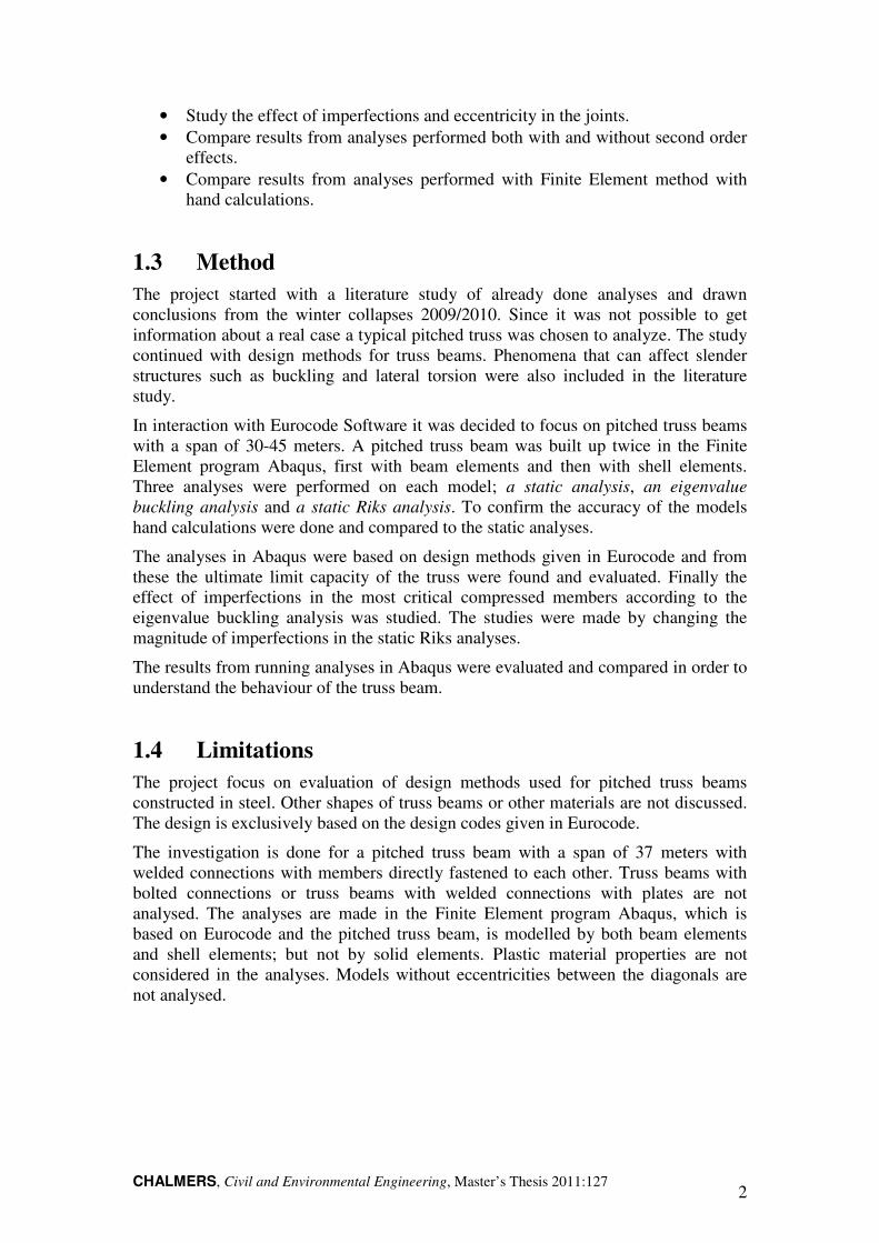
All members in the truss should be highly utilized and the loads should be transferred in an effective and safe way. A truss beam normally contains two flanges, one at the top and one at the bottom, and to transfer loads between these flanges the web is built up of a number of diagonals. The supports are normally situated at the top flange and as long as the wind load resulting in suction is smaller than the self weight, the outcome will be a compressed top flange and a bottom flange subjected to tension. The diagonals are mainly designed to resist normal forces but depending on the stiffness of the connection between diagonal and flange moments could also be transmitted. In Figure 2.1 the different members of a pitched truss beam are shown. The name of the members will be further used in this report.
Figure 2.1 Different members of a pitched truss beam.
2.1 Different types of truss beams
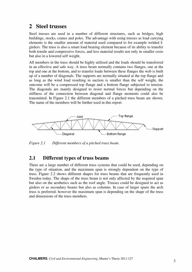
There are a large number of different truss systems that could be used, depending on the type of situation, and the maximum span is strongly dependent on the type of truss. Figure 2.2 shows different shapes for truss beams that are frequently used in Sweden today. The shape of the truss beam is not only affected by the required span but also on the aesthetics such as the roof angle. Trusses could be designed to act as girders or as secondary beams but also as columns. In case of larger spans the arch truss is preferred; however the maximum span is depending on the shape of the truss and dimensions of the truss members.
CHALMERS, Civil and Environmental Engineering, Master’s Thesis 2011:127 4
Truss beams
(a) Pitched truss
(b) Monopitched truss
(c) Inverted pitched truss
(d) Ridge truss
(e) Girder
(f) Arch truss
Figure 2.2 Different types of truss beams, Maku (2010).
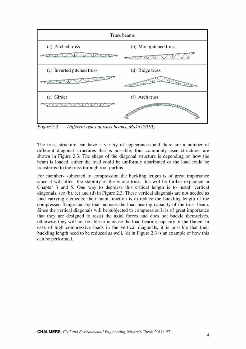
The truss structure can have a variety of appearances and there are a number of different diagonal structures that is possible; four commonly used structures are shown in Figure 2.3. The shape of the diagonal structure is depending on how the beam is loaded, either the load could be uniformly distributed or the load could be transferred to the truss through roof purlins.
For members subjected to compression the buckling length is of great importance since it will affect the stability of the whole truss, this will be further explained in Chapter 3 and 5. One way to decrease this critical length is to install vertical diagonals, see (b), (c) and (d) in Figure 2.3. These vertical diagonals are not needed as load carrying elements; their main function is to reduce the buckling length of the compressed flange and by that increase the load bearing capacity of the truss beam. Since the vertical diagonals will be subjected to compression it is of great importance that they are designed to resist the axial forces and does not buckle themselves, otherwise they will not be able to increase the load bearing capacity of the flange. In case of high compressive loads in the vertical diagonals, it is possible that their buckling length need to be reduced as well, (d) in Figure 2.3 is an example of how this can be performed.
CHALMERS, Civil and Environmental Engineering, Master’s Thesis 2011:127 5
Structures
(a) V-structure
(b) V-structure with vertical bars
(c) N-structure
(d) K-structure
Figure 2.3 Diagonals inside the truss member could be structured in different
ways depending on how the truss is designed to carry the load. The most common
used is a) V-structure, b) V-structure combined with vertical bars, c) N-structure and
d) K-structure, Thomsen (1971).
2.2 Truss elements and joints
The cross sectional shape of the flanges and the diagonals are other choices made by the designer. The choice of cross sectional shape depends for instance on the direction and character of the load and if the joints are executed with bolts or with welds. Rolled plate profiles are commonly used in steel trusses since their stiffness is large in comparison to the cross sectional area. However, in larger structures such as bridges, the height of the truss is increased which also puts demands on larger cross sectional areas of the diagonals in order to not lose critical buckling capacity in the compressed members. This demand on larger diagonals results in that it is not always enough to use rolled simple profiles, but then it is possible to create bigger cross sections with plates or rolled profiles, welded together on site.
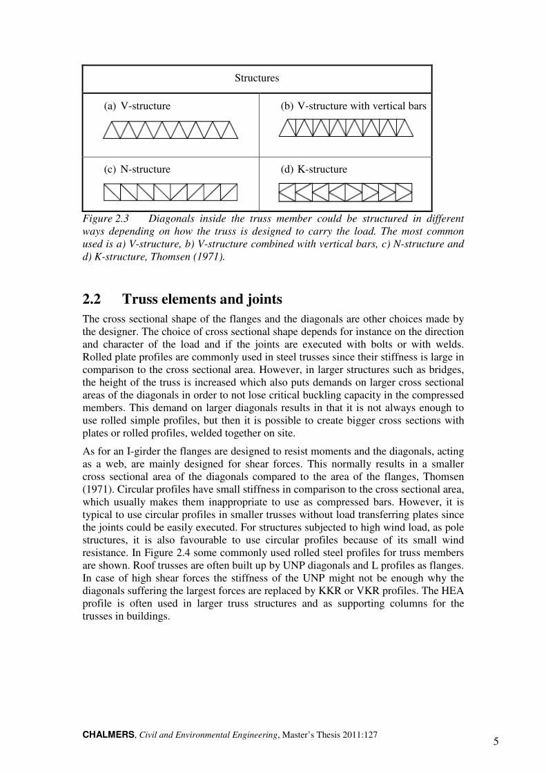
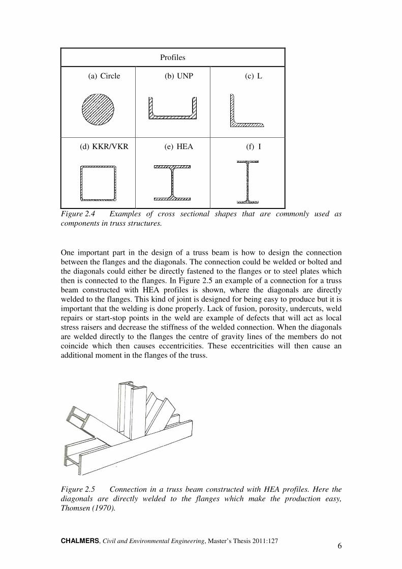
As for an I-girder the flanges are designed to resist moments and the diagonals, acting as a web, are mainly designed for shear forces. This normally results in a smaller cross sectional area of the diagonals compared to the area of the flanges, Thomsen (1971). Circular profiles have small stiffness in comparison to the cross sectional area, which usually makes them inappropriate to use as compressed bars. However, it is typical to use circular profiles in smaller trusses without load transferring plates since the joints could be easily executed. For structures subjected to high wind load, as pole structures, it is also favourable to use circular profiles because of its small wind resistance. In Figure 2.4 some commonly used rolled steel profiles for truss members are shown. Roof trusses are often built up by UNP diagonals and L profiles as flanges. In case of high shear forces the stiffness of the UNP might not be enough why the diagonals suffering the largest forces are replaced by KKR or VKR profiles. The HEA profile is often used in larger truss structures and as supporting columns for the trusses in buildings.
CHALMERS, Civil and Environmental Engineering, Master’s Thesis 2011:127 6
Profiles
(a) Circle
(b) UNP
(c) L
(d) KKR/VKR
(e) HEA
(f) I
Figure 2.4 Examples of cross sectional shapes that are commonly used as
components in truss structures.
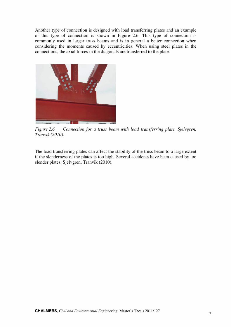
One important part in the design of a truss beam is how to design the connection between the flanges and the diagonals. The connection could be welded or bolted and the diagonals could either be directly fastened to the flanges or to steel plates which then is connected to the flanges. In Figure 2.5 an example of a connection for a truss beam constructed with HEA profiles is shown, where the diagonals are directly welded to the flanges. This kind of joint is designed for being easy to produce but it is important that the welding is done properly. Lack of fusion, porosity, undercuts, weld repairs or start-stop points in the weld are example of defects that will act as local stress raisers and decrease the stiffness of the welded connection. When the diagonals are welded directly to the flanges the centre of gravity lines of the members do not coincide which then causes eccentricities. These eccentricities will then cause an additional moment in the flanges of the truss.
Figure 2.5 Connection in a truss beam constructed with HEA profiles. Here the
diagonals are directly welded to the flanges which make the production easy,
Thomsen (1970).
CHALMERS, Civil and Environmental Engineering, Master’s Thesis 2011:127 7
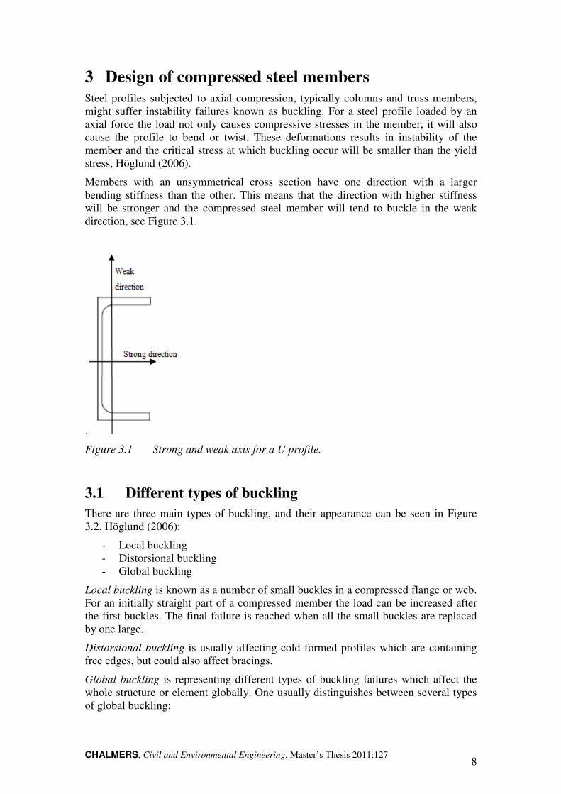
Another type of connection is designed with load transferring plates and an example of this type of connection is shown in Figure 2.6. This type of connection is commonly used in larger truss beams and is in general a better connection when considering the moments caused by eccentricities. When using steel plates in the connections, the axial forces in the diagonals are transferred to the plate.
Figure 2.6 Connection for a truss beam with load transferring plate, Sjelvgren,
Tranvik (2010).
The load transferring plates can affect the stability of the truss beam to a large extent if the slenderness of the plates is too high. Several accidents have been caused by too slender plates, Sjelvgren, Tranvik (2010).
CHALMERS, Civil and Environmental Engineering, Master’s Thesis 2011:127 8
3 Design of compressed steel members
Steel profiles subjected to axial compression, typically columns and truss members, might suffer instability failures known as buckling. For a steel profile loaded by an axial force the load not only causes compressive stresses in the member, it will also cause the profile to bend or twist. These deformations results in instability of the member and the critical stress at which buckling occur will be smaller than the yield stress, Höglund (2006).
Members with an unsymmetrical cross section have one direction with a larger bending stiffness than the other. This means that the direction with higher stiffness will be stronger and the compressed steel member will tend to buckle in the weak direction, see Figure 3.1.
.
Figure 3.1 Strong and weak axis for a U profile.
3.1 Different types of buckling
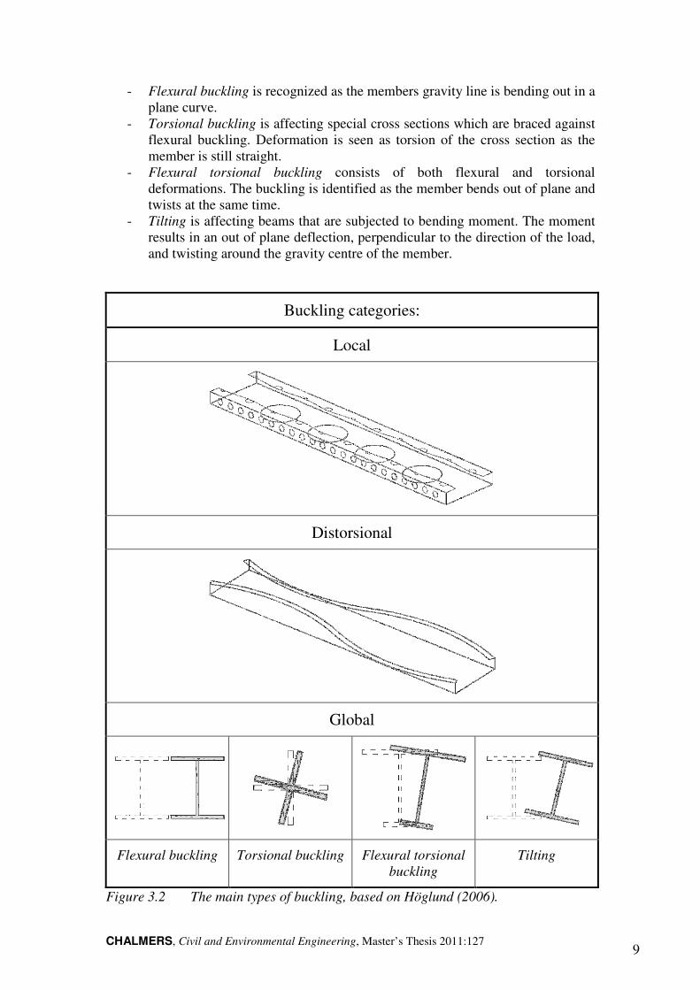
There are three main types of buckling, and their appearance can be seen in Figure 3.2, Höglund (2006):
- Local buckling - Distorsional buckling - Global buckling
Local buckling is known as a number of small buckles in a compressed flange or web. For an initially straight part of a compressed member the load can be increased after the first buckles. The final failure is reached when all the small buckles are replaced by one large.
Distorsional buckling is usually affecting cold formed profiles which are containing free edges, but could also affect bracings.
Global buckling is representing different types of buckling failures which affect the whole structure or element globally. One usually distinguishes between several types of global buckling:
CHALMERS, Civil and Environmental Engineering, Master’s Thesis 2011:127 9
- Flexural buckling is recognized as the members gravity line is bending out in a plane curve.
- Torsional buckling is affecting special cross sections which are braced against flexural buckling. Deformation is seen as torsion of the cross section as the member is still straight.
- Flexural torsional buckling consists of both flexural and torsional deformations. The buckling is identified as the member bends out of plane and twists at the same time.
- Tilting is affecting beams that are subjected to bending moment. The moment results in an out of plane deflection, perpendicular to the direction of the load, and twisting around the gravity centre of the member.
Buckling categories:
Local
Distorsional
Global
Flexural buckling Torsional buckling Flexural torsional
buckling
Tilting
Figure 3.2 The main types of buckling, based on Höglund (2006).
CHALMERS, Civil and Environmental Engineering, Master’s Thesis 2011:127 10
3.2 First order analysis - classic theory
How buckling will affect the load bearing capacity of the member is determined from the theoretical buckling load. This critical load is calculated as the load at which buckling will occur for a column which follows the classical theory. According to Höglund (2006) the assumptions for this theory are as follows:
- Linear elastic material - Small deformations - Initially completely straight member - No residual stresses
In practice these requirements are not fulfilled and the design could therefore not only rely on this theoretical buckling load.
When the material is elastic there is a stable state of equilibrium to be found for every value of the axial compressive force, Höglund (2006). But, this stable state of equilibrium is to become unstable if the deformations in the bar are too large. As the bending moments are a result of the deformations these will increase with increasing deformations and the bar will become unstable, Höglund (2006). The conclusion is that the load bearing capacity will decrease for increased deformations.
By analyzing the reasons for structures to fail in compression, it has turned out that some structures are very sensitive to imperfections. An initial deformation will give rise to additional moments which needs to be considered in the design and the residual stresses will give rise to a different stress state than the one calculated from external loading. All these parameters will affect the load bearing capacity and therefore the critical load in the classic theory need to be adjusted in order to take these effects into account, Höglund (2006).
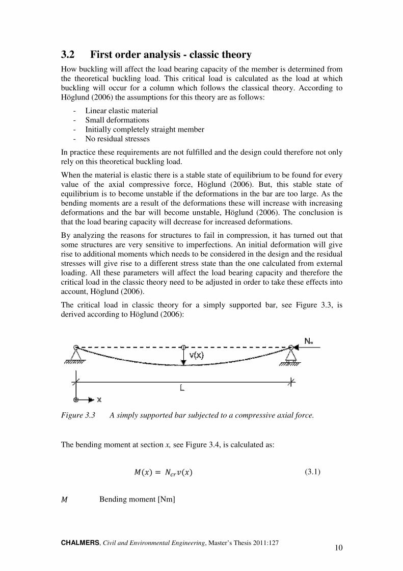
The critical load in classic theory for a simply supported bar, see Figure 3.3, is derived according to Höglund (2006):
Figure 3.3 A simply supported bar subjected to a compressive axial force.
The bending moment at section x, see Figure 3.4, is calculated as:
�234 5 ��/234 (3.1)
� Bending moment [Nm]
CHALMERS, Civil and Environmental Engineering, Master’s Thesis 2011:127 11
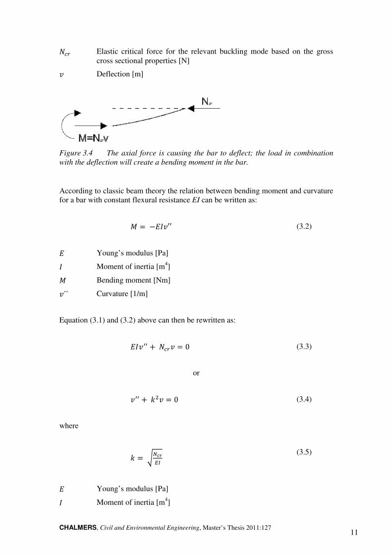
�� Elastic critical force for the relevant buckling mode based on the gross cross sectional properties [N]
/ Deflection [m]
Figure 3.4 The axial force is causing the bar to deflect; the load in combination
with the deflection will create a bending moment in the bar.
According to classic beam theory the relation between bending moment and curvature for a bar with constant flexural resistance EI can be written as:
� 56��/′′ (3.2)
� Young’s modulus [Pa]
� Moment of inertia [m4]
� Bending moment [Nm]
/´´ Curvature [1/m]
Equation (3.1) and (3.2) above can then be rewritten as:
��/88 9��/ 5 0 (3.3)
or
/88 9�;/ 5 0 (3.4)
where
� 5 <=>?�@
(3.5)
� Young’s modulus [Pa]
� Moment of inertia [m4]
CHALMERS, Civil and Environmental Engineering, Master’s Thesis 2011:127 12
�� Elastic critical force for the relevant buckling mode based on the gross cross sectional properties [N]
/ Deflection [m]
/´´ Curvature [1/m]
The general solution to Equation (3.4) is then written as:
/ 5 �AB�2�34 9 CDEA2�34 (3.6)
The equation is solved by introducing boundary conditions:
i. 3 5 0, / 5 0, which results in that B = 0 ii. 3 5 , / 5 0, results in the following expression
�AB�2�4 5 0 (3.7)
Where the solution A = 0 is representing a straight bar and the other option � 5 0 gives:
� 5 �Fwhere� 5 0, 1, 2…. (3.8)
Member length [m]
� Number of buckling mode [-]
The lowest value of �, � 5 0, is representing the case where the beam is not deflected which means that � 5 1 results in the lowest value of the load to cause deflection. The critical load according to classic theory for a pinned bar is then written as:
<=>?�@ 5 FEO�� 5PQ�@"Q
(3.9)
Or in general for other support conditions:
�� 5PQ�@">?Q (3.10)
� Young’s modulus [Pa]
CHALMERS, Civil and Environmental Engineering, Master’s Thesis 2011:127 13
� Moment of inertia [m4] Member length [m]
� Critical buckling length [m]
�� Elastic critical force for the relevant buckling mode based on the gross cross sectional properties [N]
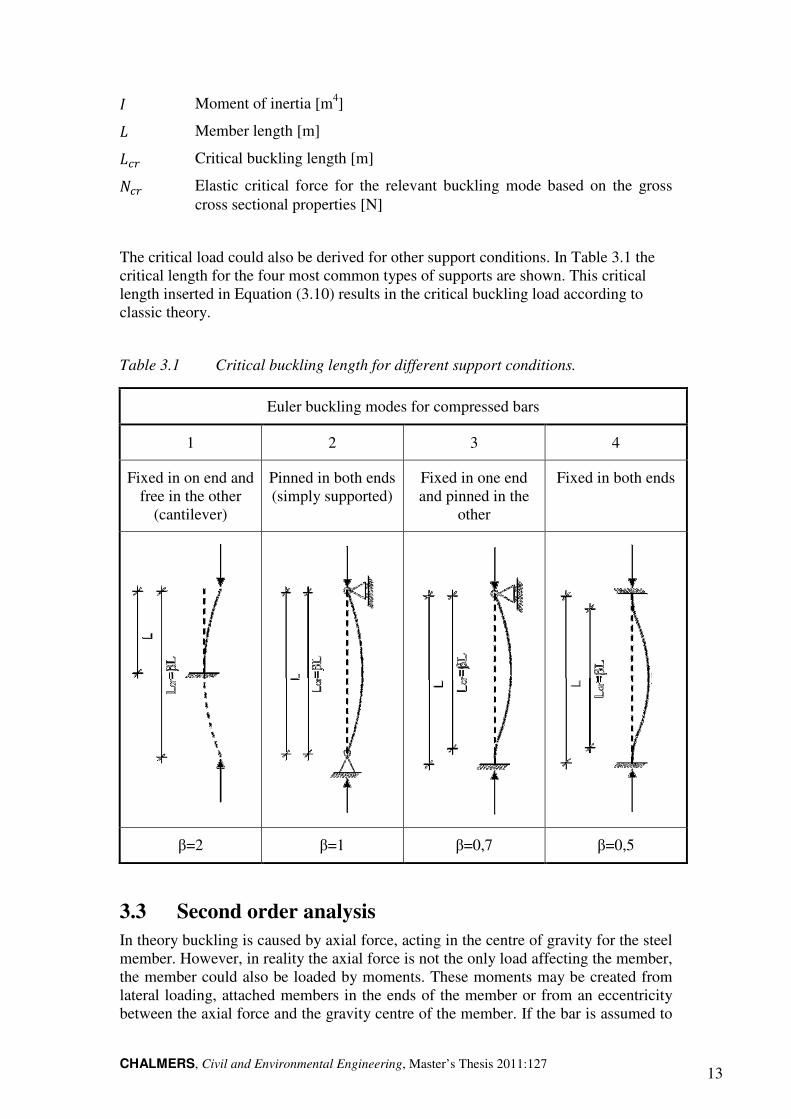
The critical load could also be derived for other support conditions. In Table 3.1 the critical length for the four most common types of supports are shown. This critical length inserted in Equation (3.10) results in the critical buckling load according to classic theory.
Table 3.1 Critical buckling length for different support conditions.
Euler buckling modes for compressed bars
1 2 3 4
Fixed in on end and free in the other
(cantilever)
Pinned in both ends (simply supported)
Fixed in one end and pinned in the
other
Fixed in both ends
β=2 β=1 β=0,7 β=0,5
3.3 Second order analysis
In theory buckling is caused by axial force, acting in the centre of gravity for the steel member. However, in reality the axial force is not the only load affecting the member, the member could also be loaded by moments. These moments may be created from lateral loading, attached members in the ends of the member or from an eccentricity between the axial force and the gravity centre of the member. If the bar is assumed to
CHALMERS, Civil and Environmental Engineering, Master’s Thesis 2011:127 14
have an initial deformation, bow imperfection, and is loaded by a compressive force, the deformation will increase in a nonlinear way with increasing load, Höglund (2006). This nonlinear deformation together with elastic material properties describes a nonlinear elastic theory or second order theory.
For a bar loaded with both an axial compressive load and moment the axial force will be multiplied with the eccentricity, created from the initial deformation of the bar, giving rise to secondary moments. This is considered in the second order analysis, which means that the relation between load and deformation is not linear. This results in that a direct solution normally cannot be calculated, instead the solution is found by iterative methods, Höglund (2006).
If the second order analysis is to be used in design of compressed members some sort of bow imperfection must be introduced. Residual stresses in the member will give rise to imperfections but this effect can normally not be considered. Some ways to consider the effect of residual stresses are given in EN 1993-1-1 (2005), see Chapter 3.4. According to Höglund (2006) the calculations are based on assumptions considering the following deviations from ideal conditions, classic theory:
- The bar has a bow imperfection - The bar is inclined (columns)
3.4 Design of compressed members according to EN 1993-
1-1
In Eurocode EN 1993-1-1 (2005) it is written that a compressed member should be verified against buckling according to the following formula:
=RS=TS
≤ 1.0 (3.11)
��� Design normal force [N]
��� Design value of the resistance to normal force [N]
According to classic theory the load at which buckling is supposed to happen for an initially straight bar, is calculated with the following expression:
�� =PQ�@">?Q (3.12)
� Young’s modulus [Pa]
� Moment of inertia [m4]
� Critical buckling length [m]
�� Elastic critical force for the relevant buckling mode based on the gross cross sectional properties [N]
CHALMERS, Civil and Environmental Engineering, Master’s Thesis 2011:127 15
The buckling length of the bar � should be based on the actual stiffness of the supports. By help from Table 3.1 the buckling length could be calculated for different support conditions.
Due to imperfections the bar will not reach the load bearing capacity calculated according to classic theory in Equation (3.12). How the buckling will affect the compressed member is depending on many factors such as how well the supports resist deformations associated with buckling, Höglund (2006). Other factors are the position of the load and how the moments in the member are distributed for a beam according to classic theory. In EN 1993-1-1 (2005) all these effects are considered in a slenderness factor V̅, and the more slender the member is, the less load is required to cause buckling.
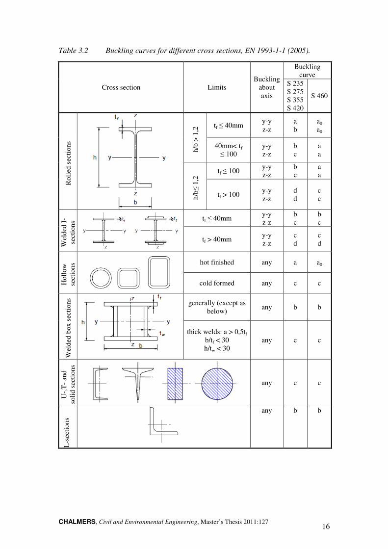
The slenderness of the compressed member is strongly affecting the buckling load. The load bearing capacity for stocky members will come close to the critical load according to classic theory and defects in the member will have minor influence. For more slender members the load bearing capacity of the member are affected by the plastic material properties and imperfections. The “real” load bearing capacity is calculated from the design curve given in EN 1993-1-1 (2005). This curve gives a relation between the relative load bearing capacity and the slenderness for bars with different cross sections and manufacturing methods.
In Table 3.2 from EN 1993-1-1 (2005) examples of different cross sections and their buckling curve are given.
CHALMERS, Civil and Environmental Engineering, Master’s Thesis 2011:127 16
Table 3.2 Buckling curves for different cross sections, EN 1993-1-1 (2005).
Cross section Limits Buckling
about axis
Buckling curve
S 235 S 275 S 355 S 420
S 460
Rol
led
sect
ions
h/b
> 1
,2 tf ≤ 40mm
y-y z-z
a b
a0
a0
40mm< tf ≤ 100
y-y z-z
b c
a a
h/b≤
1,2
tf ≤ 100 y-y z-z
b c
a a
tf > 100 y-y z-z
d d
c c
Wel
ded
I-se
ctio
ns tf ≤ 40mm
y-y z-z
b c
b c
tf > 40mm y-y z-z
c d
c d
Hol
low
se
ctio
ns hot finished any a a0
cold formed any c c
Wel
ded
box
sect
ions
generally (except as
below) any b b
thick welds: a > 0,5tf b/tf < 30 h/tw < 30
any c c
U-,
T-
and
soli
d se
ctio
ns
any c c
L-s
ecti
ons
any b b
CHALMERS, Civil and Environmental Engineering, Master’s Thesis 2011:127 17
The design buckling resistance ��,�� is given in EN 1993-1-1 (2005) by:
��,�� = XY�Z[\] forclass1, 2and3 (3.13)
��,�� = XYghh�Z[\] forclass4 (3.14)
� Cross sectional area [m2]
���� Effective cross sectional area [m2]
��,�� Design buckling resistance of a compression member [N]
�� Yield strength [Pa]
! Reduction factor for relevant buckling mode [-]
j, Partial factor for resistance of members to instability [-]
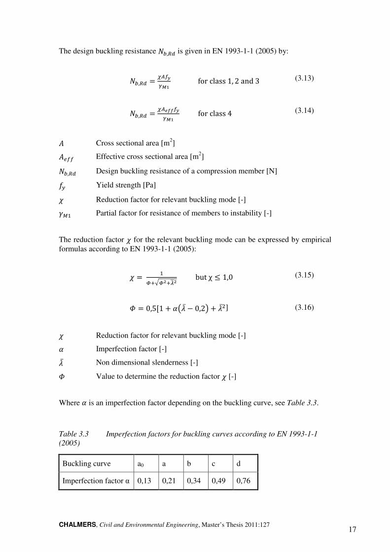
The reduction factor ! for the relevant buckling mode can be expressed by empirical formulas according to EN 1993-1-1 (2005):
! = klmkQlnoQ butχ ≤ 1,0 (3.15)
1 = 0,5[1 + $vV̅ − 0,2w + V̅;] (3.16)
! Reduction factor for relevant buckling mode [-]
$ Imperfection factor [-]
V̅ Non dimensional slenderness [-]
1 Value to determine the reduction factor ! [-]
Where $ is an imperfection factor depending on the buckling curve, see Table 3.3.
Table 3.3 Imperfection factors for buckling curves according to EN 1993-1-1
(2005)
Buckling curve a0 a b c d
Imperfection factor α 0,13 0,21 0,34 0,49 0,76
CHALMERS, Civil and Environmental Engineering, Master’s Thesis 2011:127 18
The slenderness factor V̅ is calculated with one of the following formulas depending on the cross section class of the profile:
V̅ = <Y�Z=>? forclass1, 2and3
(3.17)
V = <Yghh�Z=>? forclass4 (3.18)
� Cross sectional area [m2]
���� Effective cross sectional area [m2]
�� Elastic critical force for the relevant buckling mode based on the gross cross sectional properties [N]
�� Yield strength [Pa]
Equation (3.17) is allowable for bars in cross section class 1, 2 and 3; stress states with uniformly distributed compressive stresses. As stated in EN 1993-1-1 (2005) cross sections in class 4 will suffer local buckling before the yield stress is reached in the cross section, with the result of lowered load bearing capacity. In order to take this local buckling into account when calculating the buckling resistance of the member, the cross sectional area is reduced to an effective cross sectional area, ���� instead of
the cross sectional area �, Equation (3.18). This effective area is calculated for an effective width of the compressed member where the buckled part is reduced from the cross sectional area.
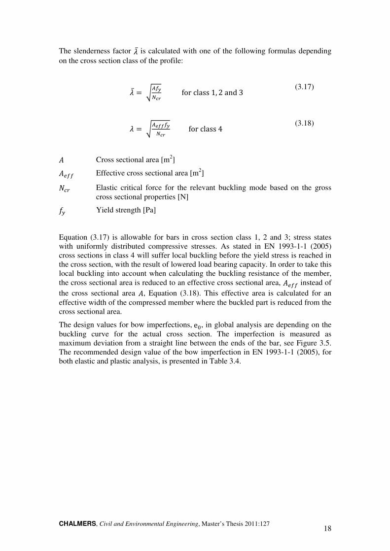
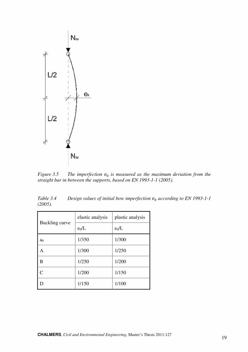
The design values for bow imperfections,e�, in global analysis are depending on the buckling curve for the actual cross section. The imperfection is measured as maximum deviation from a straight line between the ends of the bar, see Figure 3.5. The recommended design value of the bow imperfection in EN 1993-1-1 (2005), for both elastic and plastic analysis, is presented in Table 3.4.
CHALMERS, Civil and Environmental Engineering, Master’s Thesis 2011:127 19
Figure 3.5 The imperfection �� is measured as the maximum deviation from the
straight bar in between the supports, based on EN 1993-1-1 (2005).
Table 3.4 Design values of initial bow imperfection �� according to EN 1993-1-1
(2005).
Buckling curve elastic analysis plastic analysis
e0/L e0/L
a0 1/350 1/300
A 1/300 1/250
B 1/250 1/200
C 1/200 1/150
D 1/150 1/100
CHALMERS, Civil and Environmental Engineering, Master’s Thesis 2011:127 20
3.5 Design of compressed members subjected to
interaction between axial force and bending moment
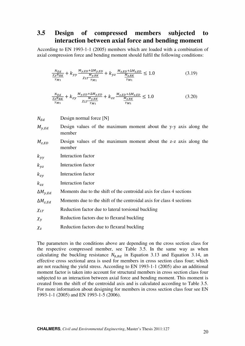
According to EN 1993-1-1 (2005) members which are loaded with a combination of axial compression force and bending moment should fulfil the following conditions:
=RSxZyTz{\]
+ ��� ,Z,R|l∆,Z,R|X}~\Z,Tz
{\]+ ��� ,�,R|l∆,�,R|
\�,Tz{\]
≤ 1.0 (3.19)
=RSx�yTz{\]
+ ��� ,Z,R|l∆,Z,R|X}~\Z,Tz
{\]+ ��� ,�,R|l∆,�,R|
\�,Tz{\]
≤ 1.0 (3.20)
��� Design normal force [N]
��,�� Design values of the maximum moment about the y-y axis along the
member
��,�� Design values of the maximum moment about the z-z axis along the member
��� Interaction factor
��� Interaction factor
��� Interaction factor
��� Interaction factor
∆��,�� Moments due to the shift of the centroidal axis for class 4 sections
∆��,�� Moments due to the shift of the centroidal axis for class 4 sections
!"# Reduction factor due to lateral torsional buckling
!� Reduction factors due to flexural buckling
!� Reduction factors due to flexural buckling
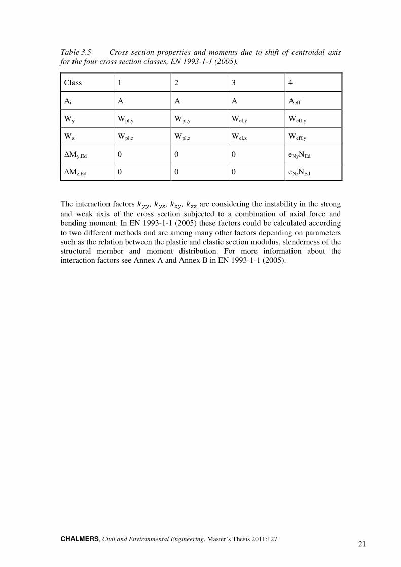
The parameters in the conditions above are depending on the cross section class for the respective compressed member, see Table 3.5. In the same way as when calculating the buckling resistance ��,�� in Equation 3.13 and Equation 3.14, an effective cross sectional area is used for members in cross section class four; which are not reaching the yield stress. According to EN 1993-1-1 (2005) also an additional moment factor is taken into account for structural members in cross section class four subjected to an interaction between axial force and bending moment. This moment is created from the shift of the centroidal axis and is calculated according to Table 3.5. For more information about designing for members in cross section class four see EN 1993-1-1 (2005) and EN 1993-1-5 (2006).
CHALMERS, Civil and Environmental Engineering, Master’s Thesis 2011:127 21
Table 3.5 Cross section properties and moments due to shift of centroidal axis
for the four cross section classes, EN 1993-1-1 (2005).
Class 1 2 3 4
Ai A A A Aeff
Wy Wpl,y Wpl,y Wel,y Weff,y
Wz Wpl,z Wpl,z Wel,z Weff,y
∆My,Ed 0 0 0 eNyNEd
∆Mz,Ed 0 0 0 eNzNEd
The interaction factors ���, ���, ���, ��� are considering the instability in the strong and weak axis of the cross section subjected to a combination of axial force and bending moment. In EN 1993-1-1 (2005) these factors could be calculated according to two different methods and are among many other factors depending on parameters such as the relation between the plastic and elastic section modulus, slenderness of the structural member and moment distribution. For more information about the interaction factors see Annex A and Annex B in EN 1993-1-1 (2005).
CHALMERS, Civil and Environmental Engineering, Master’s Thesis 2011:127 22
4 FE modelling according to classic and second
order theory with elastic and elastic-plastic
material
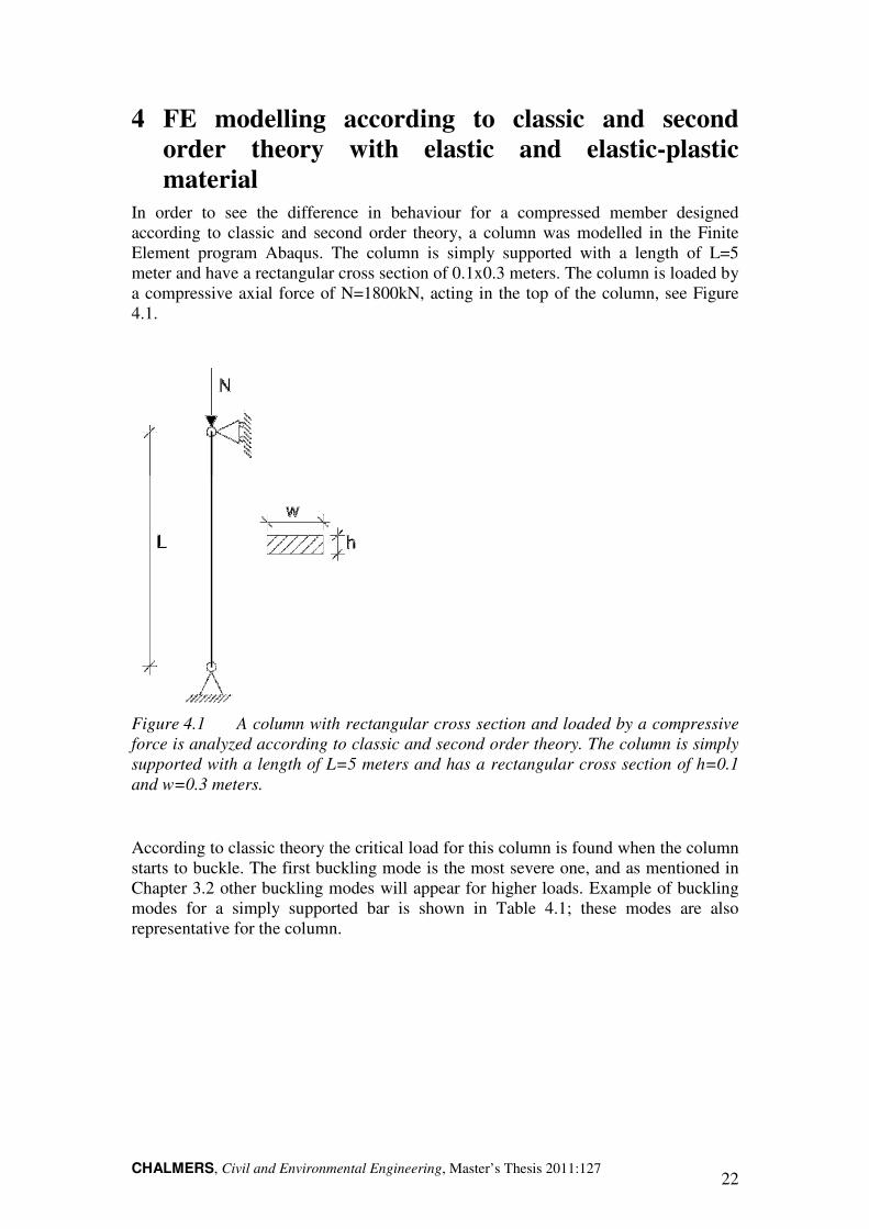
In order to see the difference in behaviour for a compressed member designed according to classic and second order theory, a column was modelled in the Finite Element program Abaqus. The column is simply supported with a length of L=5 meter and have a rectangular cross section of 0.1x0.3 meters. The column is loaded by a compressive axial force of N=1800kN, acting in the top of the column, see Figure 4.1.
Figure 4.1 A column with rectangular cross section and loaded by a compressive
force is analyzed according to classic and second order theory. The column is simply
supported with a length of L=5 meters and has a rectangular cross section of h=0.1
and w=0.3 meters.
According to classic theory the critical load for this column is found when the column starts to buckle. The first buckling mode is the most severe one, and as mentioned in Chapter 3.2 other buckling modes will appear for higher loads. Example of buckling modes for a simply supported bar is shown in Table 4.1; these modes are also representative for the column.
CHALMERS, Civil and Environmental Engineering, Master’s Thesis 2011:127 23
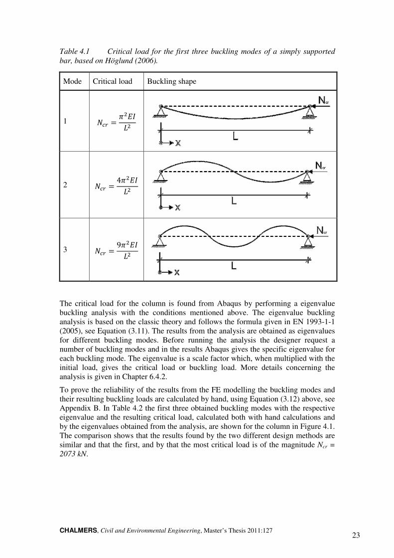
Table 4.1 Critical load for the first three buckling modes of a simply supported
bar, based on Höglund (2006).
Mode Critical load Buckling shape
1 �� = F;��;
2 �� = 4F;��;
3 �� = 9F;��;
The critical load for the column is found from Abaqus by performing a eigenvalue buckling analysis with the conditions mentioned above. The eigenvalue buckling analysis is based on the classic theory and follows the formula given in EN 1993-1-1 (2005), see Equation (3.11). The results from the analysis are obtained as eigenvalues for different buckling modes. Before running the analysis the designer request a number of buckling modes and in the results Abaqus gives the specific eigenvalue for each buckling mode. The eigenvalue is a scale factor which, when multiplied with the initial load, gives the critical load or buckling load. More details concerning the analysis is given in Chapter 6.4.2.
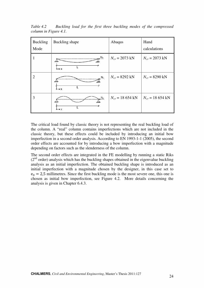
To prove the reliability of the results from the FE modelling the buckling modes and their resulting buckling loads are calculated by hand, using Equation (3.12) above, see Appendix B. In Table 4.2 the first three obtained buckling modes with the respective eigenvalue and the resulting critical load, calculated both with hand calculations and by the eigenvalues obtained from the analysis, are shown for the column in Figure 4.1. The comparison shows that the results found by the two different design methods are similar and that the first, and by that the most critical load is of the magnitude Ncr =
2073 kN.
CHALMERS, Civil and Environmental Engineering, Master’s Thesis 2011:127 24
Table 4.2 Buckling load for the first three buckling modes of the compressed
column in Figure 4.1.
Buckling
Mode
Buckling shape Abaqus Hand
calculations
1
Ncr = 2073 kN Ncr = 2073 kN
2
Ncr = 8292 kN Ncr = 8290 kN
3
Ncr = 18 654 kN Ncr = 18 654 kN
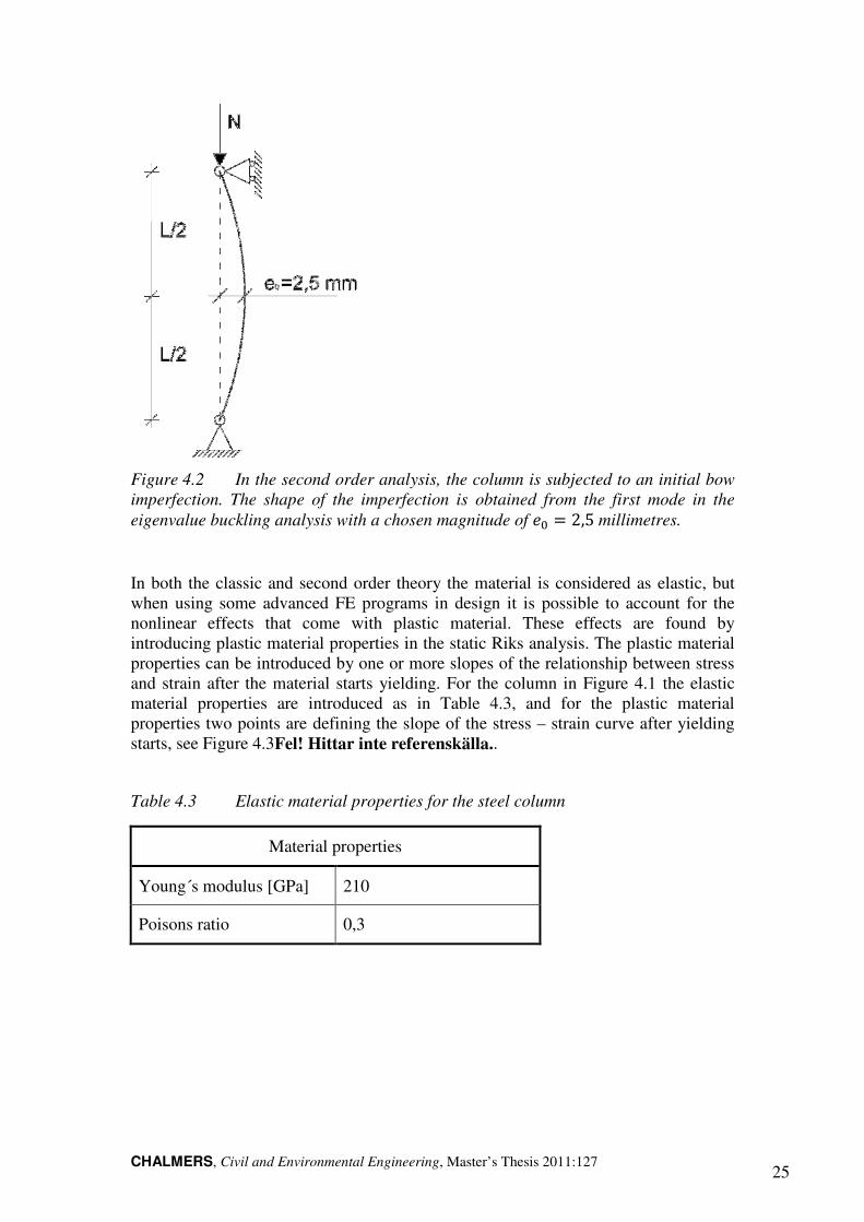
The critical load found by classic theory is not representing the real buckling load of the column. A “real” column contains imperfections which are not included in the classic theory, but these effects could be included by introducing an initial bow imperfection in a second order analysis. According to EN 1993-1-1 (2005), the second order effects are accounted for by introducing a bow imperfection with a magnitude depending on factors such as the slenderness of the column.
The second order effects are integrated in the FE modelling by running a static Riks (2nd order) analysis which has the buckling shapes obtained in the eigenvalue buckling analysis as an initial imperfection. The obtained buckling shape is introduced as an initial imperfection with a magnitude chosen by the designer, in this case set to e� = 2,5 millimetres. Since the first buckling mode is the most severe one, this one is chosen as initial bow imperfection, see Figure 4.2. More details concerning the analysis is given in Chapter 6.4.3.
CHALMERS, Civil and Environmental Engineering, Master’s Thesis 2011:127 25
Figure 4.2 In the second order analysis, the column is subjected to an initial bow
imperfection. The shape of the imperfection is obtained from the first mode in the
eigenvalue buckling analysis with a chosen magnitude of �� = 2,5 millimetres.
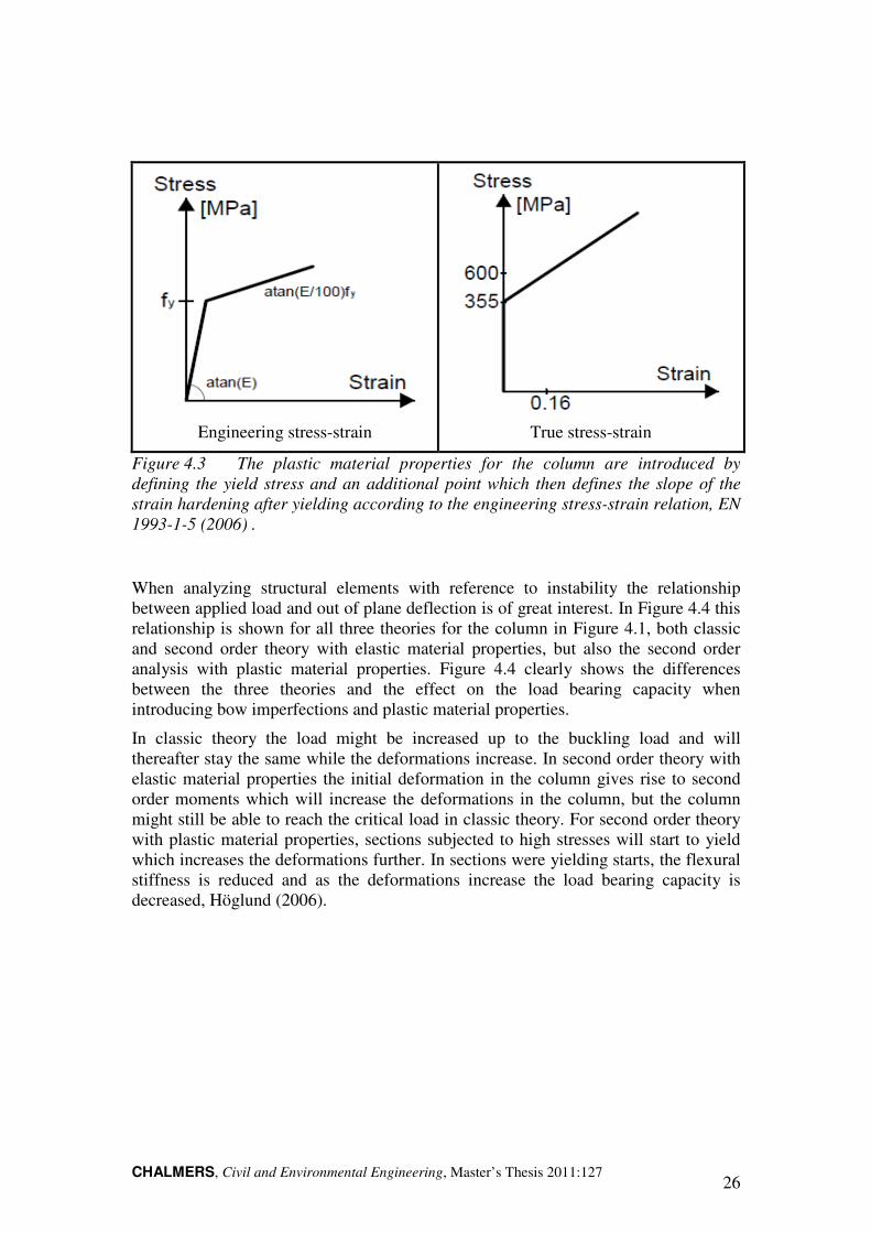
In both the classic and second order theory the material is considered as elastic, but when using some advanced FE programs in design it is possible to account for the nonlinear effects that come with plastic material. These effects are found by introducing plastic material properties in the static Riks analysis. The plastic material properties can be introduced by one or more slopes of the relationship between stress and strain after the material starts yielding. For the column in Figure 4.1 the elastic material properties are introduced as in Table 4.3, and for the plastic material properties two points are defining the slope of the stress – strain curve after yielding starts, see Figure 4.3Fel! Hittar inte referenskälla..
Table 4.3 Elastic material properties for the steel column
Material properties
Young´s modulus [GPa] 210
Poisons ratio 0,3
CHALMERS, Civil and Environmental Engineering, Master’s Thesis 2011:127 26
Engineering stress-strain
True stress-strain
Figure 4.3 The plastic material properties for the column are introduced by
defining the yield stress and an additional point which then defines the slope of the
strain hardening after yielding according to the engineering stress-strain relation, EN
1993-1-5 (2006) .
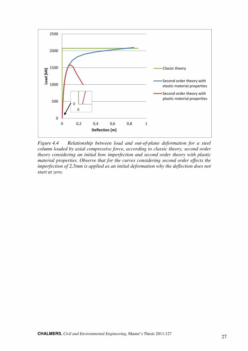
When analyzing structural elements with reference to instability the relationship between applied load and out of plane deflection is of great interest. In Figure 4.4 this relationship is shown for all three theories for the column in Figure 4.1, both classic and second order theory with elastic material properties, but also the second order analysis with plastic material properties. Figure 4.4 clearly shows the differences between the three theories and the effect on the load bearing capacity when introducing bow imperfections and plastic material properties.
In classic theory the load might be increased up to the buckling load and will thereafter stay the same while the deformations increase. In second order theory with elastic material properties the initial deformation in the column gives rise to second order moments which will increase the deformations in the column, but the column might still be able to reach the critical load in classic theory. For second order theory with plastic material properties, sections subjected to high stresses will start to yield which increases the deformations further. In sections were yielding starts, the flexural stiffness is reduced and as the deformations increase the load bearing capacity is decreased, Höglund (2006).
CHALMERS, Civil and Environmental Engineering, Master’s Thesis 2011:127 27
Figure 4.4 Relationship between load and out-of-plane deformation for a steel
column loaded by axial compressive force, according to classic theory, second order
theory considering an initial bow imperfection and second order theory with plastic
material properties. Observe that for the curves considering second order effects the
imperfection of 2,5mm is applied as an initial deformation why the deflection does not
start at zero.
0
500
1000
1500
2000
2500
0 0,2 0,4 0,6 0,8 1
Loa
d [
kN
]
Deflection [m]
Classic theory
Second order theory with
elastic material properties
Second order theory with
plastic material properties
CHALMERS, Civil and Environmental Engineering, Master’s Thesis 2011:127 28
5 Design of truss members according to EN 1993-1-1
With the ambition to lower the costs and build slimmer structures the design of a truss structure must be precise if the company should survive the competition between truss manufacturing companies. A number of different assumptions need to be made in the design and the competition between companies makes it necessary to consider these assumptions carefully since they will affect the load bearing capacity of the truss.
To get the gravity centre lines for diagonals and flanges to coincide is not always possible. Eccentricities between the centre lines give rise to moments in both flanges and diagonals. Whether these moments need to be accounted for in the design is a decision made by the designer.
The stiffness of the joints has a large impact on the design of a truss structure. The stiffer connection, the smaller buckling length can be used in the design and the higher critical buckling load is obtined. Since the connections can have a number of different configurations, it is up to the designer to assume the stiffness of the joint.
5.1 Buckling length
Each truss element is subjected to a force with a magnitude and direction depending on different load combinations and where the element is situated in the truss. This results in that some truss members are more critical than others and for the elements subjected to compression the question of buckling and instability needs to be taken into great consideration.
The buckling length of a compressed steel member is decided by the stiffness of the connection between diagonal and flange. The stiffness of a joint can be considered as somewhere in between pinned; locked in all directions but free to rotate, or as totally fixed; locked in all directions and rotations. A pinned connection corresponds to a buckling length of the entire length of the member, and a totally fixed connection corresponds to a buckling length of 0.5 times the length, see Table 3.1.
A larger buckling length results in a lower critical load according to Equation (3.12). This results in that the member is able to resist higher load before buckling starts, if the stiffness of the connection is larger. A welded connection could normally be considered to have greater stiffness than what is assumed in a pinned connection but it will be hard to create it stiff enough to consider it as fixed. When a connection is assumed to have greater stiffness than a pinned connection it is important to be aware of that if the connection starts yielding the stiffness is reduced. This reduction results in an increased buckling length than before yielding started in the joint. When the buckling length of the compressed members is increased the load to cause buckling is decreased and the members might buckle and the truss structure then fails due to instability.
5.2 Top flange subjected to compression
The applied load is important to consider when designing the top flange, not only the magnitude but how the load is transferred to the truss structure. If the truss beam is loaded through purlins the load should be considered as point loads acting in the
CHALMERS, Civil and Environmental Engineering, Master’s Thesis 2011:127 29
position of the purlins. If roof sheeting is attached to the top flange the load should be considered as uniformly distributed on the top flange.
If the beam is loaded through purlins it is necessary to consider whether the purlins are located directly over the joints between top flange and diagonals or between these joints. In the case where the purlins are located just above the joints it is only necessary to consider axial forces since no bending moment caused by loading will arise in the top flange. However, if the purlins are located between the joints or if the roof sheeting is attached directly to the top flange, the bending moment is important to consider in the design.
The top flange has to be designed for buckling as well as for axial force and bending moment and when purlins are used, both in-plane and out-of-plane buckling needs to be considered in the design. If roof sheeting is applied to the upper flange its strength could be accounted for since the roof sheeting can provide stabilization to the truss structure if it is strong enough. If the stiffness of the roof sheeting is sufficient the movement of the truss beam in the transversal direction and the rotation around longitudinal axis will be restrained, and by that the stability of the truss is increased. According to Eurocode the roof sheeting is strong enough if it is in structural class 1 or 2, Gozzi (2006). This results in that only in-plane buckling has to be checked in the design, in case of strong roof sheeting.
The compressed top flange is a built-up member and should be designed for buckling according to the method given in §6.4 EN 1993-1-1 (2005). The method is based on the assumption of hinged compressive columns which are laterally supported.
As the top chord is considered as a built-up member an effective moment of inertia is introduced and the effective critical force is calculated according to:
�� = πQ�@ghh">?Q
(5.1)
���� = 0,5ℎ�;��� (5.2)
��� Cross sectional area of the chord [m2]
E Young´s modulus [Pa]
���� The effective moment of inertia for the built-up member [m4]
� Critical buckling length [m]
ℎ� Distance of centrelines of chords for a built-up column [m]
The design value of the maximum moment in the member is calculated with consideration of second order effects. The second order effects are introduced by a bow imperfection �� with a magnitude depending on the length of the member:
��� = =RS��l,RS� �yRSy>?�
yRS��
(5.3)
CHALMERS, Civil and Environmental Engineering, Master’s Thesis 2011:127 30
�� = "��� (5.4)
Member length [m]
��� Design value of the maximum moment in the middle of the built-up member, considering second order effects [Nm]
��� Design value of the maximum moment in the middle of the built-up member, without considering second order effects [Nm]
�� Elastic critical force for the relevant buckling mode based on the gross cross sectional properties [N]
��� Design normal force [N]
�� Shear stiffness of built-up member from the lacings or battened panel [N]
�� Maximum amplitude of a member imperfection [m]
As the maximum moment is known, the design axial force ���,�� for two identical truss chords with consideration of an initial bow imperfection could be calculated. This design force should then be compared to the design resistance of the flange.
���,�� = 0.5��� + ,RS��Y>�;@ghh (5.5)
=>�,RS=�,TS
≤ 1,0 (5.6)
��� Cross sectional area of the chord [m2]
���� The effective moment of inertia for the built up member [m4]
��� Design value of the maximum moment in the middle of the built-up member, considering second order effects [Nm]
��,�� Design buckling resistance of a compression member [N]
���,�� Design chord force in the middle of a built-up member, for two identical chords [N]
��� Design normal force [N]
ℎ� Distance of centrelines of chords for a built-up column [m]
5.3 Bottom flange
For the most common truss structures the top flange is in compression and the bottom flange is in tension, however some circumstances can cause the opposite. As an example, wind load for a low pitched truss can cause external suction or internal
CHALMERS, Civil and Environmental Engineering, Master’s Thesis 2011:127 31
pressure within the building which can result in a compressed bottom chord. This reverse loading situation is very important to consider in the design. The load bearing capacity for a compressed member is significantly lowered compared to a tensioned member due to buckling instability.
5.4 Diagonals
Depending on the stiffness of the joints, the critical buckling length of the compressed diagonal is somewhere in between 0.5 and 1 length of the bar. When designing the diagonal, the buckling length is of great importance both for in-plane and out-of-plane buckling, Thomsen (1971). As mentioned in Chapter 5.1, the actual stiffness of the connection is hard to decide and it is important to make sure that the assumption is on the safe side. If a too low stiffness is accounted for, the structure is going to be larger and more expensive than necessary. In case of the opposite the structure could collapse for a lower load than expected due to buckling of critical elements.
The diagonals can be considered as Euler columns loaded only by an axial force and checks of in-plane and out-of-plane buckling are necessary to make. As mentioned above the effective length depends on the design of the joint but also the shape of the cross section. According to EN 1993-1-1 (2005) the value of the buckling length should be taken as equal to the total length for all cross sections, unless a smaller value can be justified by analysis.
5.5 Imperfections
Imperfections are created in structural components in many different ways. During the manufacturing and erection of a structure mistakes can be made and deformations in an initially straight member could easily be created in storage or handling of the member. The mistakes can have an impact on the performance of the truss structure and depending on the magnitude and sensitivity of the member it should be included in the design. Residual stresses can be present in the steel member and there can also be geometrical imperfections in the structure. The members themselves can have a lack of verticality, lack of straightness or a lack of flatness. The structural components can also be constructed with a lack of fit and minor eccentricities, EN 1993-1-1 (2005). All these defects can create a different moment distribution and results in lowering of the load bearing capacity.
In EN 1993-1-1 (2005) it is recommended to introduce a bow imperfection to take the defects mentioned above, into account when analyzing the critical compressed members in the truss. The bow imperfection depends on three things; the cross section of the member, the length of the member and if the analysis is elastic or plastic. The cross section of the member decides which buckling curve to be used. From this curve, depending on the length of the member and whether the analysis is considering elastic or plastic material, the recommended bow imperfection is obtained, see Chapter 3.4.
CHALMERS, Civil and Environmental Engineering, Master’s Thesis 2011:127 32
5.6 Eccentricity
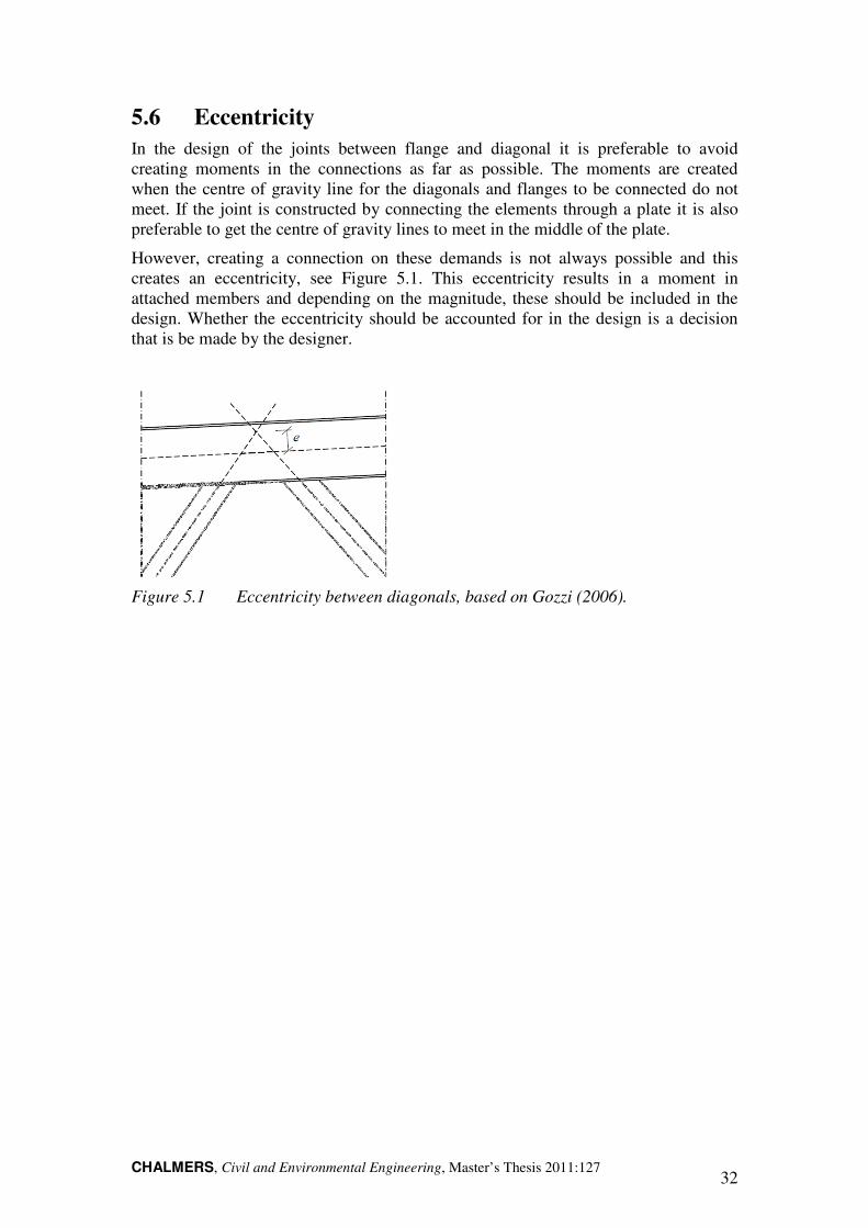
In the design of the joints between flange and diagonal it is preferable to avoid creating moments in the connections as far as possible. The moments are created when the centre of gravity line for the diagonals and flanges to be connected do not meet. If the joint is constructed by connecting the elements through a plate it is also preferable to get the centre of gravity lines to meet in the middle of the plate.
However, creating a connection on these demands is not always possible and this creates an eccentricity, see Figure 5.1. This eccentricity results in a moment in attached members and depending on the magnitude, these should be included in the design. Whether the eccentricity should be accounted for in the design is a decision that is be made by the designer.
Figure 5.1 Eccentricity between diagonals, based on Gozzi (2006).
CHALMERS, Civil and Environmental Engineering, Master’s Thesis 2011:127 33
6 Modelling of truss beam in Abaqus
In order to ease the understanding of the performance of a truss beam and the effect of buckling, a pitched truss beam was modelled in the Finite Element program Abaqus. This truss beam was modelled both with beam and shell elements in order to see the differences in buckling modes and behaviour. The analysis includes sensibility against imperfections by introducing different magnitudes of initial bow imperfections.
6.1 Input data for truss beam
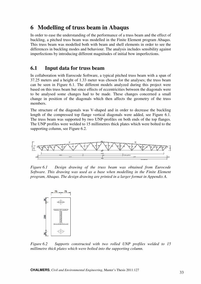
In collaboration with Eurocode Software, a typical pitched truss beam with a span of 37.25 meters and a height of 1.33 meter was chosen for the analyses; the truss beam can be seen in Figure 6.1. The different models analyzed during this project were based on this truss beam but since effects of eccentricities between the diagonals were to be analysed some changes had to be made. These changes concerned a small change in position of the diagonals which then affects the geometry of the truss members.
The structure of the diagonals was V-shaped and in order to decrease the buckling length of the compressed top flange vertical diagonals were added, see Figure 6.1. The truss beam was supported by two UNP-profiles on both ends of the top flanges. The UNP profiles were welded to 15 millimetres thick plates which were bolted to the supporting column, see Figure 6.2.
Figure 6.1 Design drawing of the truss beam was obtained from Eurocode
Software. This drawing was used as a base when modelling in the Finite Element
program, Abaqus. The design drawing are printed in a larger format in Appendix A.
Figure 6.2 Supports constructed with two rolled UNP profiles welded to 15
millimetre thick plates which were bolted into the supporting column.
CHALMERS, Civil and Environmental Engineering, Master’s Thesis 2011:127 34
In Table 6.1 the section profiles for all members in the modelled truss beam are listed. The number for each element can be seen in Figure 6.1. The top and bottom flanges are constructed with L120x120x13 and L120x120x11 profiles respectively and all diagonals except the two compressed ones closest to the supports are constructed with UNP 120 profiles. Near the supports the truss is subjected to high shear forces which make the diagonals close to the support more critical. To increase the capacity of the truss beam diagonals 6 and 39, see Figure 6.1, were constructed with KKR 120x120x5.0 profiles which have a higher critical buckling load than UNP 120 profiles.
Table 6.1 Profiles of the elements are listed. The element numbers can be seen in
Figure 6.1.
Element number Profile
01-02 L 120x120x13.0
03 L 120x120x11.0
04 + 41 Support plate 150x300x15, 2xUNP 120
05 + 07-38 + 40 UNP 120
06 + 39 KKR 120x120x5.0
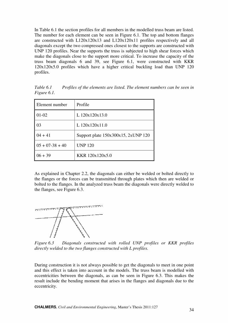
As explained in Chapter 2.2, the diagonals can either be welded or bolted directly to the flanges or the forces can be transmitted through plates which then are welded or bolted to the flanges. In the analyzed truss beam the diagonals were directly welded to the flanges, see Figure 6.3.
Figure 6.3 Diagonals constructed with rolled UNP profiles or KKR profiles
directly welded to the two flanges constructed with L profiles.
During construction it is not always possible to get the diagonals to meet in one point and this effect is taken into account in the models. The truss beam is modelled with eccentricities between the diagonals, as can be seen in Figure 6.3. This makes the result include the bending moment that arises in the flanges and diagonals due to the eccentricity.
CHALMERS, Civil and Environmental Engineering, Master’s Thesis 2011:127 35
6.2 Beam elements
The truss beam was first modelled in Abaqus using beam elements. A model with beam elements can analyze both global and local buckling of the structure. However, these elements are not able to analyze the local buckling of the cross sectional area, which is important to keep in mind when analyzing the results. The advantage with using beam elements is the small amount of time needed for Abaqus to analyze and give results. It is therefore preferable to use this type of elements if changes needs to be done in the model, and since results could be obtained quite fast the designer is able to make changes in the model by testing. If a large model is about to be analyzed in Abaqus it is therefore recommended starting modelling with beam elements and when the program and behaviour of the model is familiar to the user, continue with other types of elements.
When modelling in Abaqus it is important to decide which units that should be used in order to obtain correct results. For the analyzed truss beam meter [m], Newton [N] and Pascal [Pa] was chosen.
6.2.1 Geometry
When using beam elements the first step is to draw path lines representing the length of the member. The path lines representing the members are created one by one and are assembled together later. Exact coordinates can be given to the path lines when created, which makes the assembling easier when the lines are getting their right position immediately. Another way to create an assembly is to create the path lines without their exact coordinates and move the lines into their exact position during the assembling. Since every diagonal has a unique angle in the truss beam to be analysed the exact coordinates were given to the path lines directly.
6.2.2 Properties
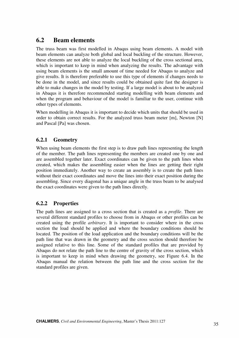
The path lines are assigned to a cross section that is created as a profile. There are several different standard profiles to choose from in Abaqus or other profiles can be created using the profile arbitrary. It is important to consider where in the cross section the load should be applied and where the boundary conditions should be located. The position of the load application and the boundary conditions will be the path line that was drawn in the geometry and the cross section should therefore be assigned relative to this line. Some of the standard profiles that are provided by Abaqus do not relate the path line to the centre of gravity of the cross section, which is important to keep in mind when drawing the geometry, see Figure 6.4. In the Abaqus manual the relation between the path line and the cross section for the standard profiles are given.
CHALMERS, Civil and Environmental Engineering, Master’s Thesis 2011:127 36
Location of path line for
Abaqus standard profiles Location of path line for the truss
analysis, defined in arbitrary section
Figure 6.4 Localisation of path line for an L profile.
For the analyzed truss beam the load should be applied and the boundary conditions located in the gravity centre. It was therefore only possible to use the standard profile for the KKR profile since this had the path line located in the centre of gravity of the cross section. The UNP profile does not exist as a standard profile in Abaqus and the L profile does not have the path line located in the gravity centre. The UNP profile and the L profiles were created as the profile arbitrary. When drawing your own profiles it is important to create the profile with its path line located in the gravity centre. Origin represents the location of the path line. As a simplification the rounded corners was excluded for both L profiles and UNP profile. However, the centre of gravity and flexural resistance were controlled to be similar for the cross section with rounded corners and the cross section without, see hand calculations in Appendix B.
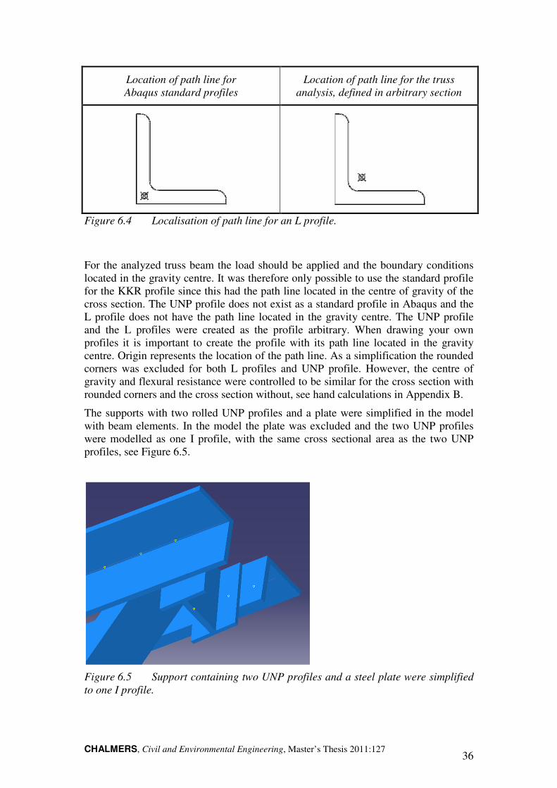
The supports with two rolled UNP profiles and a plate were simplified in the model with beam elements. In the model the plate was excluded and the two UNP profiles were modelled as one I profile, with the same cross sectional area as the two UNP profiles, see Figure 6.5.
Figure 6.5 Support containing two UNP profiles and a steel plate were simplified
to one I profile.
CHALMERS, Civil and Environmental Engineering, Master’s Thesis 2011:127 37
When modelling with beam elements all sections are represented by simple lines. However, as a control that the path lines have their right cross section and oriented in a correct way the model could be displayed with its cross sections as in Figure 6.5. To display the model with its cross-section use view/assembly display options/render
beam profiles.
The path lines that represent the members are also assigned to a material. The material is created with different properties such as density, elastic- and plastic properties. The self weight of the truss beam was excluded and no density was applied to the material properties for the truss beam. For all analyses elastic properties with Young modulus and Poisson’s ratio were applied similar to the steel column, see Table 4.3.
6.2.3 Step
When creating a model an initial step already exists. In this step are all initial conditions for the model created, such as boundary conditions. A new step that decides which type of analysis that should be performed on the model needs to be created. Usually only one step is created for each model. In the created step the information concerning the requested analysis is given, for example magnitude of the load which should be applied to the structure and the requested output.
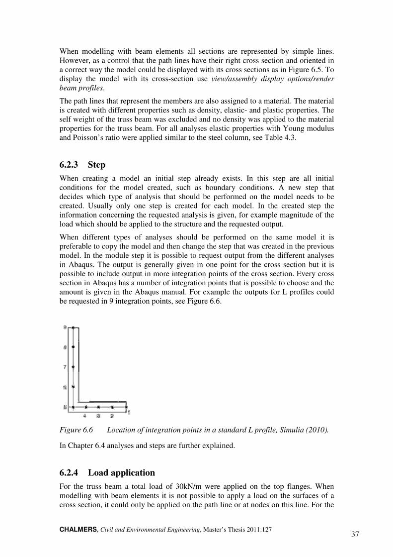
When different types of analyses should be performed on the same model it is preferable to copy the model and then change the step that was created in the previous model. In the module step it is possible to request output from the different analyses in Abaqus. The output is generally given in one point for the cross section but it is possible to include output in more integration points of the cross section. Every cross section in Abaqus has a number of integration points that is possible to choose and the amount is given in the Abaqus manual. For example the outputs for L profiles could be requested in 9 integration points, see Figure 6.6.
Figure 6.6 Location of integration points in a standard L profile, Simulia (2010).
In Chapter 6.4 analyses and steps are further explained.
6.2.4 Load application
For the truss beam a total load of 30kN/m were applied on the top flanges. When modelling with beam elements it is not possible to apply a load on the surfaces of a cross section, it could only be applied on the path line or at nodes on this line. For the
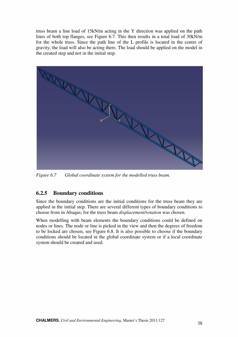
CHALMERS, Civil and Environmental Engineering, Master’s Thesis 2011:127 38
truss beam a line load of 15kN/m acting in the Y direction was applied on the path lines of both top flanges, see Figure 6.7. This then results in a total load of 30kN/m for the whole truss. Since the path line of the L profile is located in the centre of gravity, the load will also be acting there. The load should be applied on the model in the created step and not in the initial step.
Figure 6.7 Global coordinate system for the modelled truss beam.
6.2.5 Boundary conditions
Since the boundary conditions are the initial conditions for the truss beam they are applied in the initial step. There are several different types of boundary conditions to choose from in Abaqus; for the truss beam displacement/rotation was chosen.
When modelling with beam elements the boundary conditions could be defined on nodes or lines. The node or line is picked in the view and then the degrees of freedom to be locked are chosen, see Figure 6.8. It is also possible to choose if the boundary conditions should be located in the global coordinate system or if a local coordinate system should be created and used.
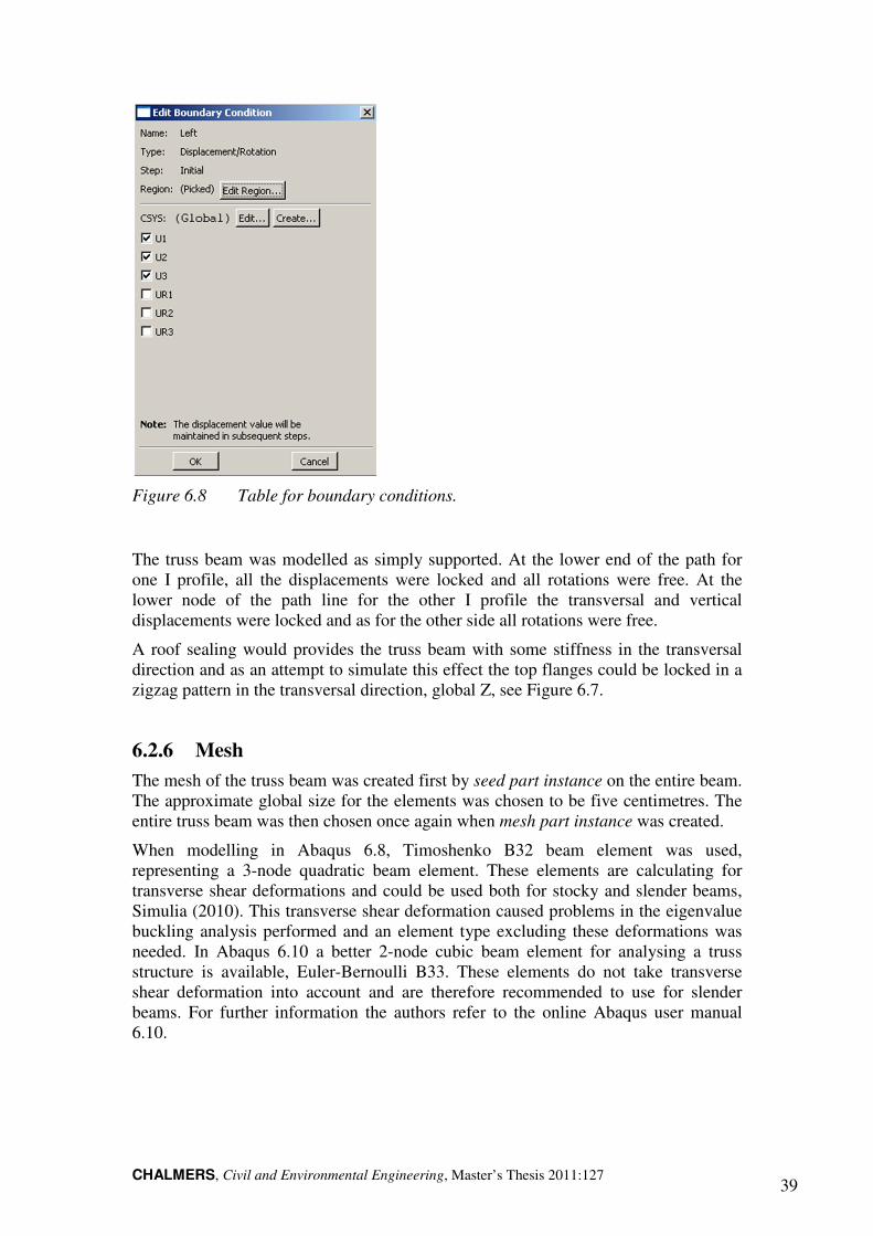
CHALMERS, Civil and Environmental Engineering, Master’s Thesis 2011:127 39
Figure 6.8 Table for boundary conditions.
The truss beam was modelled as simply supported. At the lower end of the path for one I profile, all the displacements were locked and all rotations were free. At the lower node of the path line for the other I profile the transversal and vertical displacements were locked and as for the other side all rotations were free.
A roof sealing would provides the truss beam with some stiffness in the transversal direction and as an attempt to simulate this effect the top flanges could be locked in a zigzag pattern in the transversal direction, global Z, see Figure 6.7.
6.2.6 Mesh
The mesh of the truss beam was created first by seed part instance on the entire beam. The approximate global size for the elements was chosen to be five centimetres. The entire truss beam was then chosen once again when mesh part instance was created.
When modelling in Abaqus 6.8, Timoshenko B32 beam element was used, representing a 3-node quadratic beam element. These elements are calculating for transverse shear deformations and could be used both for stocky and slender beams, Simulia (2010). This transverse shear deformation caused problems in the eigenvalue buckling analysis performed and an element type excluding these deformations was needed. In Abaqus 6.10 a better 2-node cubic beam element for analysing a truss structure is available, Euler-Bernoulli B33. These elements do not take transverse shear deformation into account and are therefore recommended to use for slender beams. For further information the authors refer to the online Abaqus user manual 6.10.
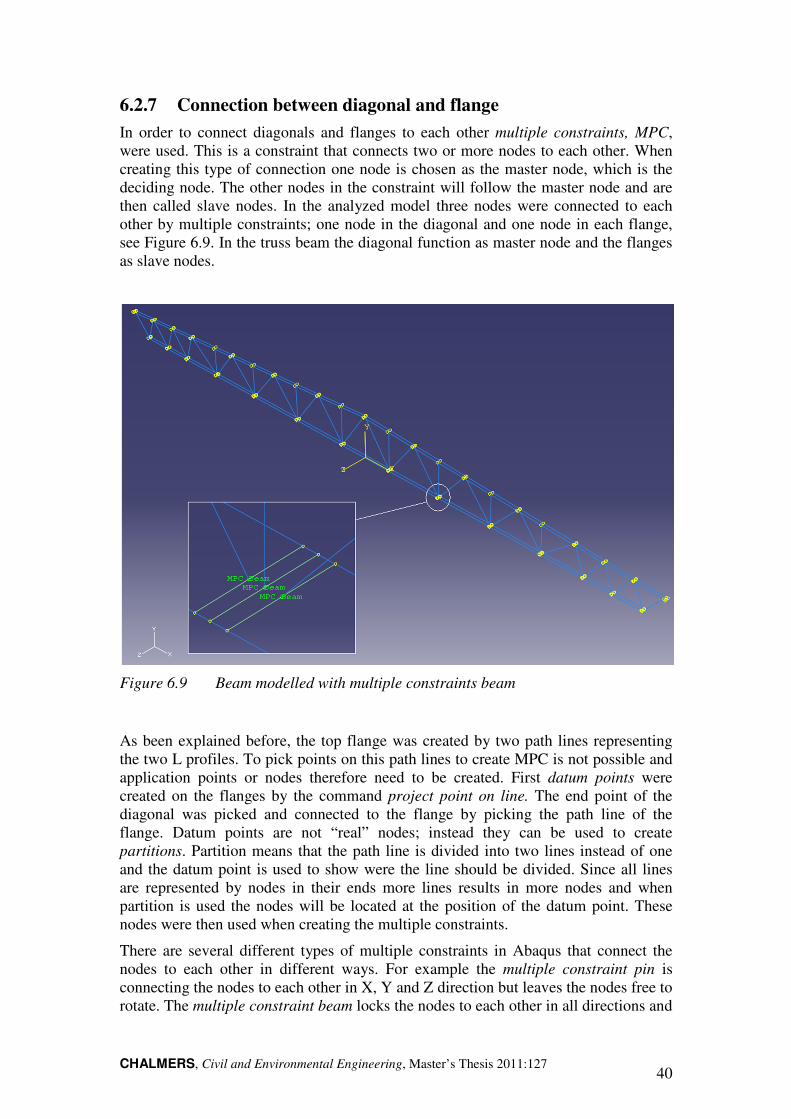
CHALMERS, Civil and Environmental Engineering, Master’s Thesis 2011:127 40
6.2.7 Connection between diagonal and flange
In order to connect diagonals and flanges to each other multiple constraints, MPC, were used. This is a constraint that connects two or more nodes to each other. When creating this type of connection one node is chosen as the master node, which is the deciding node. The other nodes in the constraint will follow the master node and are then called slave nodes. In the analyzed model three nodes were connected to each other by multiple constraints; one node in the diagonal and one node in each flange, see Figure 6.9. In the truss beam the diagonal function as master node and the flanges as slave nodes.
Figure 6.9 Beam modelled with multiple constraints beam
As been explained before, the top flange was created by two path lines representing the two L profiles. To pick points on this path lines to create MPC is not possible and application points or nodes therefore need to be created. First datum points were created on the flanges by the command project point on line. The end point of the diagonal was picked and connected to the flange by picking the path line of the flange. Datum points are not “real” nodes; instead they can be used to create partitions. Partition means that the path line is divided into two lines instead of one and the datum point is used to show were the line should be divided. Since all lines are represented by nodes in their ends more lines results in more nodes and when partition is used the nodes will be located at the position of the datum point. These nodes were then used when creating the multiple constraints.
There are several different types of multiple constraints in Abaqus that connect the nodes to each other in different ways. For example the multiple constraint pin is connecting the nodes to each other in X, Y and Z direction but leaves the nodes free to rotate. The multiple constraint beam locks the nodes to each other in all directions and
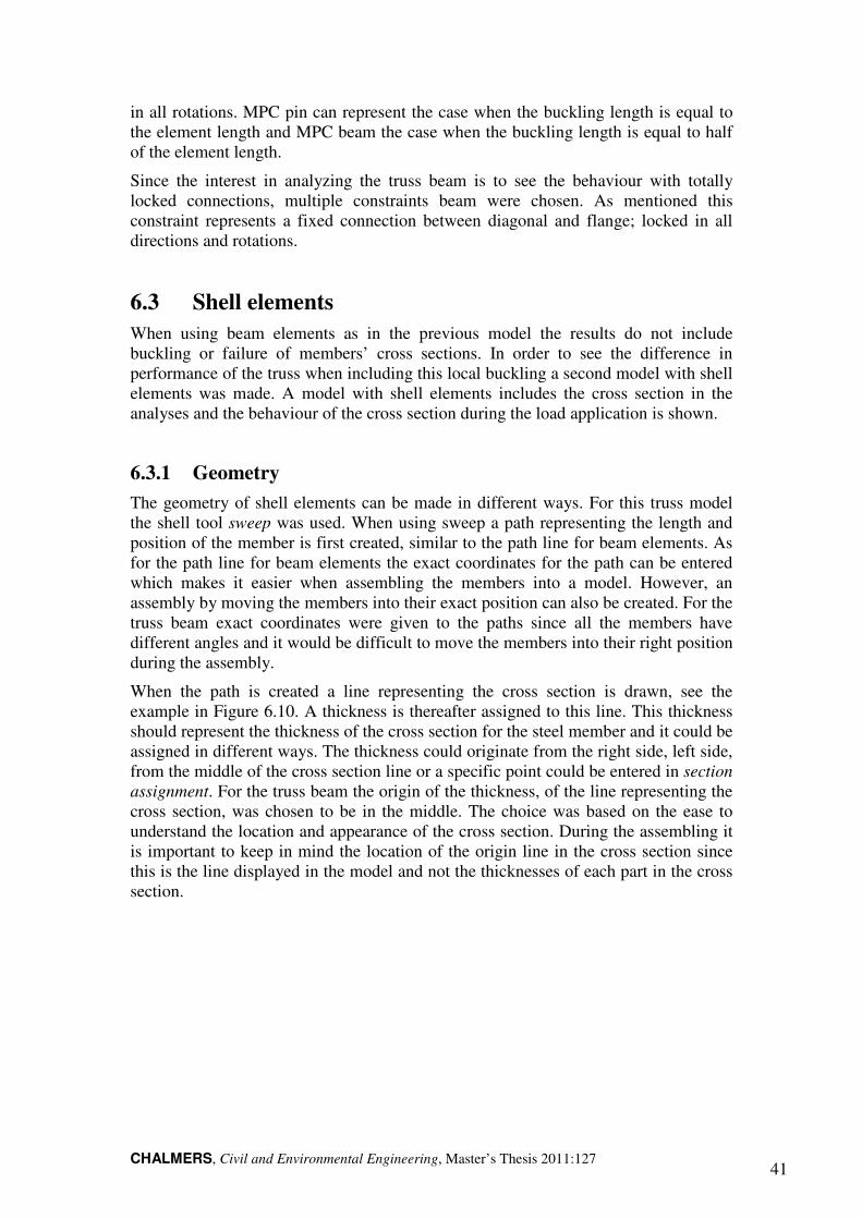
CHALMERS, Civil and Environmental Engineering, Master’s Thesis 2011:127 41
in all rotations. MPC pin can represent the case when the buckling length is equal to the element length and MPC beam the case when the buckling length is equal to half of the element length.
Since the interest in analyzing the truss beam is to see the behaviour with totally locked connections, multiple constraints beam were chosen. As mentioned this constraint represents a fixed connection between diagonal and flange; locked in all directions and rotations.
6.3 Shell elements
When using beam elements as in the previous model the results do not include buckling or failure of members’ cross sections. In order to see the difference in performance of the truss when including this local buckling a second model with shell elements was made. A model with shell elements includes the cross section in the analyses and the behaviour of the cross section during the load application is shown.
6.3.1 Geometry
The geometry of shell elements can be made in different ways. For this truss model the shell tool sweep was used. When using sweep a path representing the length and position of the member is first created, similar to the path line for beam elements. As for the path line for beam elements the exact coordinates for the path can be entered which makes it easier when assembling the members into a model. However, an assembly by moving the members into their exact position can also be created. For the truss beam exact coordinates were given to the paths since all the members have different angles and it would be difficult to move the members into their right position during the assembly.
When the path is created a line representing the cross section is drawn, see the example in Figure 6.10. A thickness is thereafter assigned to this line. This thickness should represent the thickness of the cross section for the steel member and it could be assigned in different ways. The thickness could originate from the right side, left side, from the middle of the cross section line or a specific point could be entered in section
assignment. For the truss beam the origin of the thickness, of the line representing the cross section, was chosen to be in the middle. The choice was based on the ease to understand the location and appearance of the cross section. During the assembling it is important to keep in mind the location of the origin line in the cross section since this is the line displayed in the model and not the thicknesses of each part in the cross section.
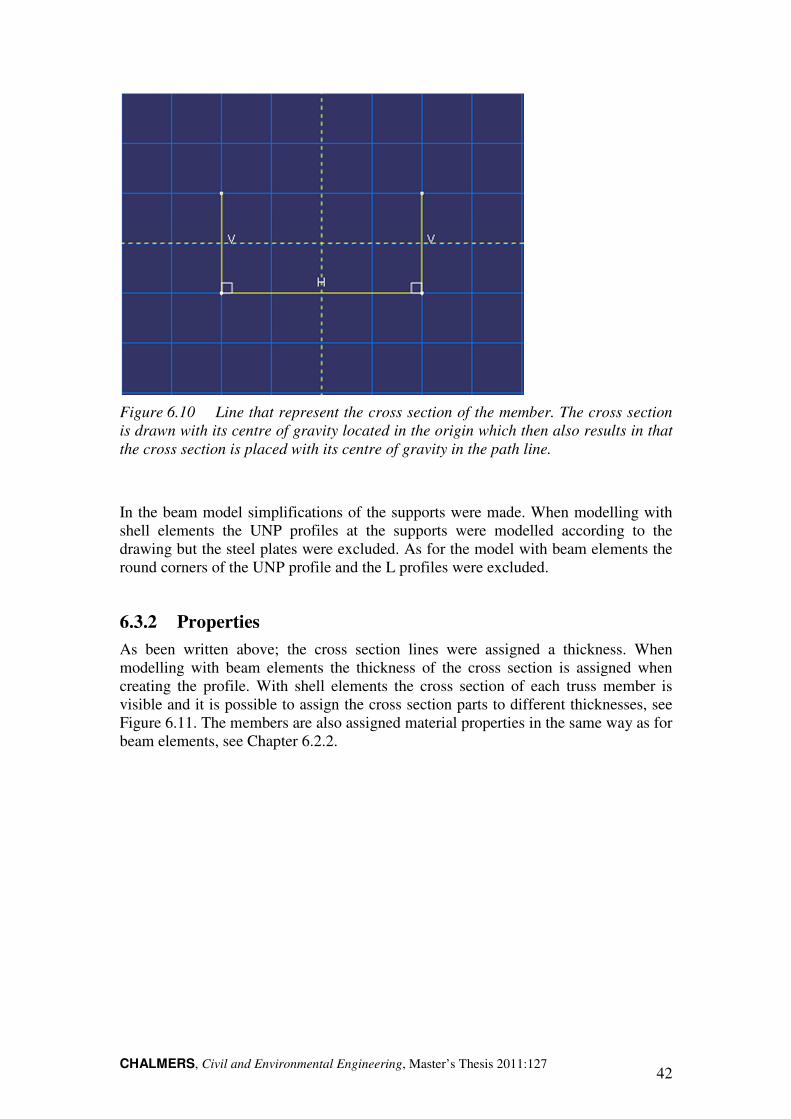
CHALMERS, Civil and Environmental Engineering, Master’s Thesis 2011:127 42
Figure 6.10 Line that represent the cross section of the member. The cross section
is drawn with its centre of gravity located in the origin which then also results in that
the cross section is placed with its centre of gravity in the path line.
In the beam model simplifications of the supports were made. When modelling with shell elements the UNP profiles at the supports were modelled according to the drawing but the steel plates were excluded. As for the model with beam elements the round corners of the UNP profile and the L profiles were excluded.
6.3.2 Properties
As been written above; the cross section lines were assigned a thickness. When modelling with beam elements the thickness of the cross section is assigned when creating the profile. With shell elements the cross section of each truss member is visible and it is possible to assign the cross section parts to different thicknesses, see Figure 6.11. The members are also assigned material properties in the same way as for beam elements, see Chapter 6.2.2.
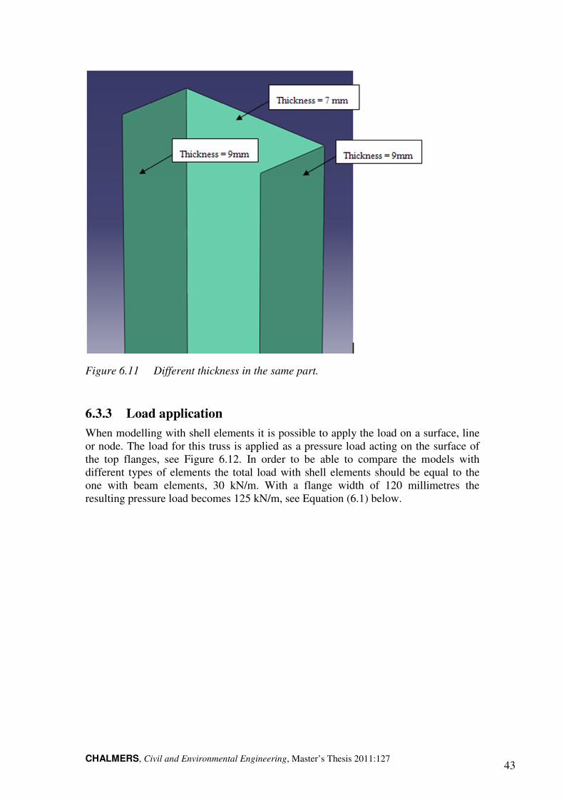
CHALMERS, Civil and Environmental Engineering, Master’s Thesis 2011:127 43
Figure 6.11 Different thickness in the same part.
6.3.3 Load application
When modelling with shell elements it is possible to apply the load on a surface, line or node. The load for this truss is applied as a pressure load acting on the surface of the top flanges, see Figure 6.12. In order to be able to compare the models with different types of elements the total load with shell elements should be equal to the one with beam elements, 30 kN/m. With a flange width of 120 millimetres the resulting pressure load becomes 125 kN/m, see Equation (6.1) below.
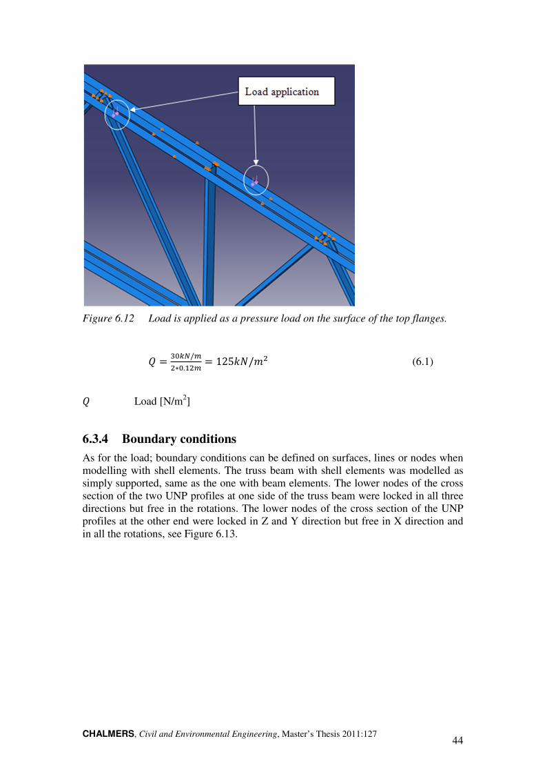
CHALMERS, Civil and Environmental Engineering, Master’s Thesis 2011:127 44
Figure 6.12 Load is applied as a pressure load on the surface of the top flanges.
� = ��+=/�;∗�. ;� = 125��/�; (6.1)
� Load [N/m2]
6.3.4 Boundary conditions
As for the load; boundary conditions can be defined on surfaces, lines or nodes when modelling with shell elements. The truss beam with shell elements was modelled as simply supported, same as the one with beam elements. The lower nodes of the cross section of the two UNP profiles at one side of the truss beam were locked in all three directions but free in the rotations. The lower nodes of the cross section of the UNP profiles at the other end were locked in Z and Y direction but free in X direction and in all the rotations, see Figure 6.13.
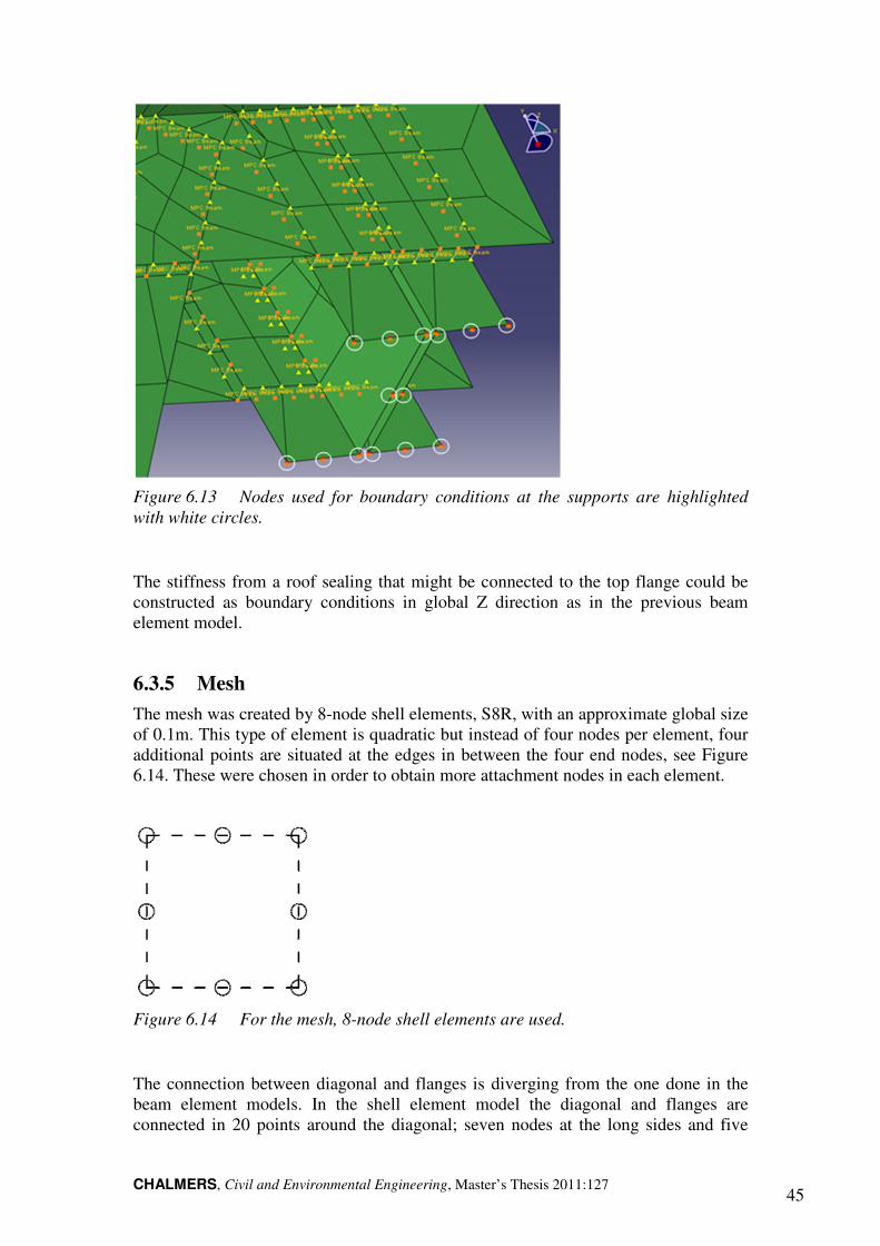
CHALMERS, Civil and Environmental Engineering, Master’s Thesis 2011:127 45
Figure 6.13 Nodes used for boundary conditions at the supports are highlighted
with white circles.
The stiffness from a roof sealing that might be connected to the top flange could be constructed as boundary conditions in global Z direction as in the previous beam element model.
6.3.5 Mesh
The mesh was created by 8-node shell elements, S8R, with an approximate global size of 0.1m. This type of element is quadratic but instead of four nodes per element, four additional points are situated at the edges in between the four end nodes, see Figure 6.14. These were chosen in order to obtain more attachment nodes in each element.
Figure 6.14 For the mesh, 8-node shell elements are used.
The connection between diagonal and flanges is diverging from the one done in the beam element models. In the shell element model the diagonal and flanges are connected in 20 points around the diagonal; seven nodes at the long sides and five
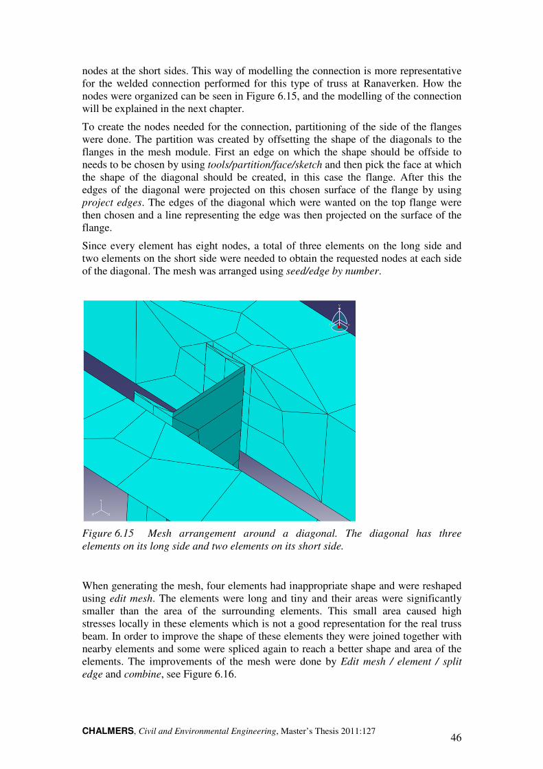
CHALMERS, Civil and Environmental Engineering, Master’s Thesis 2011:127 46
nodes at the short sides. This way of modelling the connection is more representative for the welded connection performed for this type of truss at Ranaverken. How the nodes were organized can be seen in Figure 6.15, and the modelling of the connection will be explained in the next chapter.
To create the nodes needed for the connection, partitioning of the side of the flanges were done. The partition was created by offsetting the shape of the diagonals to the flanges in the mesh module. First an edge on which the shape should be offside to needs to be chosen by using tools/partition/face/sketch and then pick the face at which the shape of the diagonal should be created, in this case the flange. After this the edges of the diagonal were projected on this chosen surface of the flange by using project edges. The edges of the diagonal which were wanted on the top flange were then chosen and a line representing the edge was then projected on the surface of the flange.
Since every element has eight nodes, a total of three elements on the long side and two elements on the short side were needed to obtain the requested nodes at each side of the diagonal. The mesh was arranged using seed/edge by number.
Figure 6.15 Mesh arrangement around a diagonal. The diagonal has three
elements on its long side and two elements on its short side.
When generating the mesh, four elements had inappropriate shape and were reshaped using edit mesh. The elements were long and tiny and their areas were significantly smaller than the area of the surrounding elements. This small area caused high stresses locally in these elements which is not a good representation for the real truss beam. In order to improve the shape of these elements they were joined together with nearby elements and some were spliced again to reach a better shape and area of the elements. The improvements of the mesh were done by Edit mesh / element / split
edge and combine, see Figure 6.16.

CHALMERS, Civil and Environmental Engineering, Master’s Thesis 2011:127 47
Figure 6.16 Mesh editing.
An input file for the model was written and then imported back to the program. This creates a new model with fixed geometrical properties. The reason for this was to make mesh nodes possible to pick for load, boundary conditions and connections. In the truss beam the nodes in the mesh were used to create the connection between diagonal and flange.
6.3.6 Connection between diagonal and flange
The connection between diagonal and flange is performed in a more realistic way than in the model with beam elements. In reality the weld is performed all around the diagonal, see Figure 6.17. In the model the weld was performed using multiple constraints beam, the same constraints as in the beam model. As been explained before; multiple constraints connect two or more nodes to each other. The weld in the model with shell elements was simulated with seven constraints on the long sides and five constraints on the short sides. This way of connecting the truss members was considered as better representation of the real weld instead of using only one constraint as in the beam element model, see Figure 6.18. One constraint will cause high stresses locally at the constraint and by using more constraints the stresses are evened out.
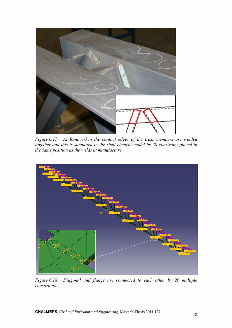
CHALMERS, Civil and Environmental Engineering, Master’s Thesis 2011:127 48
Figure 6.17 At Ranaverken the contact edges of the truss members are welded
together and this is simulated in the shell element model by 20 constraint placed in
the same position as the welds at manufacture.
Figure 6.18 Diagonal and flange are connected to each other by 20 multiple
constraints.
CHALMERS, Civil and Environmental Engineering, Master’s Thesis 2011:127 49
The multiple constraints could have been created in the same way as for the model with beam elements; create a MPC, pick the master node and then pick the slave nodes. However, this process is very time consuming and the model with shell elements contains a very large number of constraints. Instead of creating the MPC one by one MPC beam was created as a connector section. In connector section there are many different standard connections to be chosen. For the truss beam MPC beam was chosen since the connection between diagonal and flange should be totally fixed as in the beam element model. When multiple constraints are used as a connector section no nodes will be assigned as master or slave nodes, instead all nodes are equal.
The connector sections should thereafter be assigned to a wire. Wires between the node in the diagonal and the node in the flange are created. Many wires can be created at once which results in a wire set. The entire wire set could thereafter be assigned to the connector section and the multiple constraints beam are assigned, see Figure 6.18. The nodes picked for the wires are the mesh nodes that were created along with the mesh.
6.4 Analyses in Abaqus
Three different analyses were performed on the models; a static analysis, an eigenvalue buckling analysis and a static Riks analysis. The different analyses are created by the choice of step. It is preferred that each model contains only the initial step and the created step. The model was therefore copied and the step changed, before running the analysis. When a step is changed the load needs to be recreated since the load is created in the step that was deleted. If boundary conditions are not assigned in the initial step, these also need to be redone.
6.4.1 Static analysis
The static analyses were performed to confirm the accuracy of the models, and the step static, general was used for this purpose. The load in this model was not performed as a line load or as a pressure; instead a concentrated load was applied in the middle node of both flanges. The static analysis was not performed to see the behaviour of the truss beam and the application of the load was therefore performed in a way which made the comparison between hand calculations and results obtained from Abaqus easier. The results from these analyses confirmed that the reaction forces in the supports were equal the applied load, for both the beam- and shell element model.
6.4.2 Eigenvalue buckling analysis
Eigenvalue buckling analysis, with the step linear perturbation buckle, was performed on the models. This analysis calculates the possible buckling modes and their eigenvalue. The buckling modes represent different buckling scenarios for compressed members in the truss and the first mode is the most critical.
When creating the step linear perturbation buckle, the number of buckling modes is chosen. For both the beam- and shell element model 25 buckling modes were requested, this number covered the buckling modes of interest. For this type of analysis it is possible to choose between two types of eigensolvers; Lanczos and
CHALMERS, Civil and Environmental Engineering, Master’s Thesis 2011:127 50
Subspace. In the truss analyses Lanczos was chosen as eigensolver together with the request of 25 positive buckling modes.
The buckling analysis is only possible to perform on stiff structures and the truss beam can be considered as a stiff structure since the diagonals and flanges act like Euler columns Simulia (2010). The eigenvalue buckling analysis can be used to estimate the critical buckling load but can also be used to provide the static Riks analysis with information. The buckling analysis is in this case used as input data for the static Riks analysis. If the buckling analysis should be used as an input data the results need to be saved. This is made by typing the following words, before end step in keywords for the model with the step linear perturbation buckle:
*NODE FILE, GLOBAL=YES, LAST MODE= {number of requested buckling modes}
U
6.4.3 Static Riks analysis
The second order effects and imperfections are integrated in the FE modelling by running the step static Riks. By introducing imperfections in the model, possible faults made at manufactory or at site are taken into account which results in a more realistic load bearing behaviour of the truss. The load is applied gradually and the results show how the behaviour of the truss changes until failure occurs. From these results the failure load is possible to find for the modelled truss beam.
The eigenvalue buckling analysis provides the static Riks analysis with information about the shape of the buckling modes for the most critical elements in the truss. The obtained buckling shape is then introduced as an initial imperfection in critical members of the truss with a magnitude chosen by the designer. These initial bow imperfections are included in the analysis by writing the following words before step in keyword, for the model with the step static Riks:
*IMPERFECTION, FILE={name of the job for the buckling analysis}, STEP=1
{number of the first buckling mode}, {magnitude of imperfection}
{number of the second buckling mode}, { magnitude of imperfection }
etcetera
The list of buckling modes and imperfections in keywords can be as long as needed. In the modelling of the truss beam only two imperfections were introduced. The magnitude of the imperfections was based on EN 1993-1-1 (2005), see Chapter 5.5.
With the static Riks analysis it is possible to choose if the analysis should include the second order effects or not. This is made by turning Nlgeom on or off when editing the step or in the job table, sees Figure 6.19.
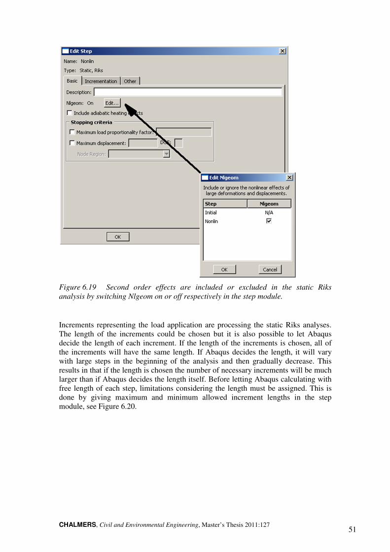
CHALMERS, Civil and Environmental Engineering, Master’s Thesis 2011:127 51
Figure 6.19 Second order effects are included or excluded in the static Riks
analysis by switching Nlgeom on or off respectively in the step module.
Increments representing the load application are processing the static Riks analyses. The length of the increments could be chosen but it is also possible to let Abaqus decide the length of each increment. If the length of the increments is chosen, all of the increments will have the same length. If Abaqus decides the length, it will vary with large steps in the beginning of the analysis and then gradually decrease. This results in that if the length is chosen the number of necessary increments will be much larger than if Abaqus decides the length itself. Before letting Abaqus calculating with free length of each step, limitations considering the length must be assigned. This is done by giving maximum and minimum allowed increment lengths in the step module, see Figure 6.20.
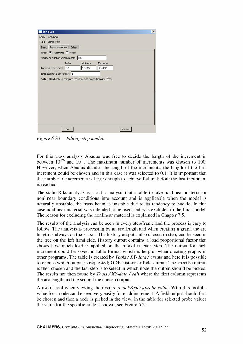
CHALMERS, Civil and Environmental Engineering, Master’s Thesis 2011:127 52
Figure 6.20 Editing step module.
For this truss analysis Abaqus was free to decide the length of the increment in between 10-26 and 1035. The maximum number of increments was chosen to 100. However, when Abaqus decides the length of the increments, the length of the first increment could be chosen and in this case it was selected to 0.1. It is important that the number of increments is large enough to achieve failure before the last increment is reached.
The static Riks analysis is a static analysis that is able to take nonlinear material or nonlinear boundary conditions into account and is applicable when the model is naturally unstable; the truss beam is unstable due to its tendency to buckle. In this case nonlinear material was intended to be used, but was excluded in the final model. The reason for excluding the nonlinear material is explained in Chapter 7.5.
The results of the analysis can be seen in every step/frame and the process is easy to follow. The analysis is processing by an arc length and when creating a graph the arc length is always on the x-axis. The history outputs, also chosen in step, can be seen in the tree on the left hand side. History output contains a load proportional factor that shows how much load is applied on the model at each step. The output for each increment could be saved in table format which is helpful when creating graphs in other programs. The table is created by Tools / XY-data / create and here it is possible to choose which output is requested; ODB history or field output. The specific output is then chosen and the last step is to select in which node the output should be picked. The results are then found by Tools / XY-data / edit where the first column represents the arc length and the second the chosen output.
A useful tool when viewing the results is tools/query/probe value. With this tool the value for a node can be seen very easily for each increment. A field output should first be chosen and then a node is picked in the view; in the table for selected probe values the value for the specific node is shown, see Figure 6.21.
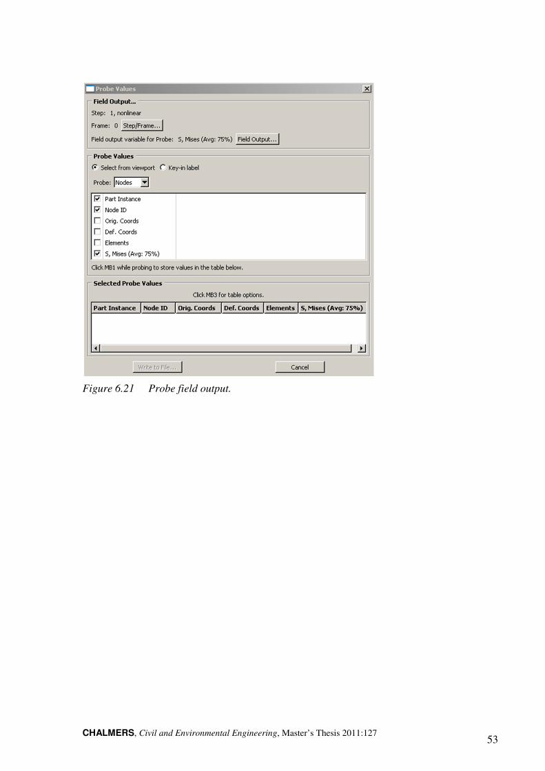
CHALMERS, Civil and Environmental Engineering, Master’s Thesis 2011:127 53
Figure 6.21 Probe field output.
CHALMERS, Civil and Environmental Engineering, Master’s Thesis 2011:127 54
7 Problems
A number of modelling problems in Abaqus have been solved during this project. Some of the problems were minor and easily solved, by help from other people at the division of steel and timber structures or by reading in the Simulia (2010); other problems were major and took hours of researching to solve. A few problems have been left unsolved during this project. This chapter will explain the problems that occurred and the solutions that were found. During the modelling shortcuts that made the work easier were found and some of these will also be explained in this chapter.
7.1 Geometry
The most important concern when modelling in Abaqus is to create a model that does not include faults of any kind, such as errors in the geometry. The first thing to consider is which units should be used. These units have to be used consistently throughout the entire work.
One of the largest problems in this work occurred when the beam model was created. Some standard profiles in Abaqus are not modelled in their gravity centre. This issue caused problems twice and both times the entire model needed to be changed. When modelling with beam elements the members are represented by path lines and the cross sections are not shown. At the beginning of the modelling the cross sections of the members were created by standard profiles in the belief that the cross sections were modelled in their gravity centre. When the possibility to see the cross sections was found, in view/assembly display options/render beam profiles, it was clear that the members had the wrong position. This problem was taken care of by moving the members into their right position in assembly.
However, it is not enough to get the cross sections into their right position. The boundary conditions and the load are neither located in the gravity centre. This problem was found when the results from the analyses were evaluated. Tensioned members were deformed as subjected to compression and additional moments created from the eccentricity between gravity centre and load application were found. Since new profiles with their path line in the gravity centre needed to be created and the members’ position changed; a completely new model was created.
An issue that came up when creating own profiles were how the rounded corners should be created. This problem was not solved. Instead a new profile without rounded corners but with similar moment of inertia and flexural resistance as the standard profile was created, see Appendix B.
In Abaqus members of the truss were created one by one and assembled together later. The truss beam contains several members with different angels and positions. In the first model the members were moved into their right position in assembly. This is possible to do but it is very difficult and time consuming when working in such a complicated model as the truss beam. The second time the model was created exact coordinates for the members were entered directly when the members were created. In this way the members got into their right position directly when assembled.
In the beginning of the work in Abaqus the modelling was very time consuming. However, during the work shortcuts were found; an example of this is how to use and create datum points. Datum points are not nodes of the members but a node can be
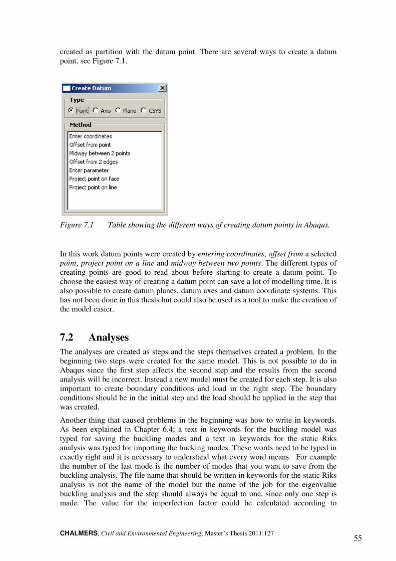
CHALMERS, Civil and Environmental Engineering, Master’s Thesis 2011:127 55
created as partition with the datum point. There are several ways to create a datum point, see Figure 7.1.
Figure 7.1 Table showing the different ways of creating datum points in Abaqus.
In this work datum points were created by entering coordinates, offset from a selected point, project point on a line and midway between two points. The different types of creating points are good to read about before starting to create a datum point. To choose the easiest way of creating a datum point can save a lot of modelling time. It is also possible to create datum planes, datum axes and datum coordinate systems. This has not been done in this thesis but could also be used as a tool to make the creation of the model easier.
7.2 Analyses
The analyses are created as steps and the steps themselves created a problem. In the beginning two steps were created for the same model. This is not possible to do in Abaqus since the first step affects the second step and the results from the second analysis will be incorrect. Instead a new model must be created for each step. It is also important to create boundary conditions and load in the right step. The boundary conditions should be in the initial step and the load should be applied in the step that was created.
Another thing that caused problems in the beginning was how to write in keywords. As been explained in Chapter 6.4; a text in keywords for the buckling model was typed for saving the buckling modes and a text in keywords for the static Riks analysis was typed for importing the bucking modes. These words need to be typed in exactly right and it is necessary to understand what every word means. For example the number of the last mode is the number of modes that you want to save from the buckling analysis. The file name that should be written in keywords for the static Riks analysis is not the name of the model but the name of the job for the eigenvalue buckling analysis and the step should always be equal to one, since only one step is made. The value for the imperfection factor could be calculated according to
CHALMERS, Civil and Environmental Engineering, Master’s Thesis 2011:127 56
Eurocode or if the sensibility against imperfections should be analysed, it could be chosen randomly.
7.3 Different versions of Abaqus
At the division of steel and timber structures different versions of Abaqus exists. This limits people to help each other and it can also cause problems when it is needed to change version during work. This thesis started with working in version 6.8. Since there showed to exist some errors in version 6.8 that could cause problems with the buckling modes; the model was tested in version 6.7. In version 6.8 it is possible to use multiple constraints, MPC, but in version 6.7 MPC does not exist and then all constraints just disappeared in the model. This caused a stability problem when running the analysis. To figure out that the lack of multiple constraints caused this problem was very time consuming.
The buckling analysis results in buckling modes and their respective eigenvalue. When analysing the results from the eigenvalue buckling analysis of the beam model it showed that a diagonal buckled with one, two and even more sinus curves with nearly exactly the same eigenvalue. This phenomenon is not possible since the force needed for a compressed member to buckle in higher modes would be significantly greater than the first mode. A question was sent to Abaqus support and the answer showed that the wrong element type was used. The element type B32 could make the transverse shear stiffness too low and their recommendation was to change the element type to B33, in order to exclude shear deformations. The solution seemed simple but after some research it turned out that B33 does not exist in version 6.8; that was used for the analyses. A change to version 6.10 was made. When the elements were changed to B33 the results from the eigenvalue buckling analysis seemed correct. However, when the eigenvalue buckling analysis worked properly a new problem was found in the static Riks analysis. This new problem was not solved and will be explained further in Chapter 7.7.
7.4 Error messages
When running a job that contains faults, error occurs and an error message is received. These error messages that contains information about what caused the error can sometimes be hard to understand. An explanation of some of the error messages that have been received during this work follows.
An error message that is usual to get is that conflicts occurs in keywords. This error is easy to fix; the rows that contain the words conflict need to be deleted from keywords. After this is done; the analysis can be submitted once again without this problem.
It is also usual to get a stability problem. This means that a member or members are not constrained enough. When this error message is received it is important to go through the model in detail and figure out what can cause this error. In the beginning of the thesis it was decided that a truss beam with pinned connections should be analysed. This model would simulate a case with the buckling length equal to the total system length of the truss members. This was executed by using multiple constraint pin. When using this constraint an error message containing stability problems was received. An answer to this instability error is believed to be problem with the
CHALMERS, Civil and Environmental Engineering, Master’s Thesis 2011:127 57
constraints. A pinned constraint allows the members to rotate and the truss members then started to rotate around their own longitudinal axis, which then caused instability.
7.5 Different trials
One of the aims at the beginning of this thesis was to check how the behaviour of the structure changed for different buckling lengths. There have been several attempts to investigate this behaviour but in the end this investigation was cancelled due to other time consuming problems with Abaqus. The attempts that has been made is explained in this chapter.
As been said in the previous chapter was an attempt made with MPC pin instead of MPC beam in the beam model. This would represent the case when the connections between diagonal and flange were pinned. This caused a stability problem since the members were able to rotate around their own axis.
Instead of using MPC pin a coupling connection was tried, which locked the connection in all directions and rotations except around the transversal axis. Around the transversal axis a rotational spring was used. However, after a lot of research it was found that the coupling connection did not work like it was assumed. The coupling connection does not connect two or more nodes to each other as a multiple constraint; it connects several of nodes to a point that could be located anywhere.
To avoid this problem MPC pin was used again but with additional rotational springs around all three axes. The springs that were used could be chosen to work in all directions and around all axes but only one can be chosen each time, so the springs are either translational or rotational. When MPC pin was used; springs should be used around all three axes and since only one rotation could be chosen three springs were used. The stiffness of the springs could be changed and this should make it possible to see the behaviour of the structure for different magnitudes of stiffness of the joints. At this time the problem with Abaqus not modelling in the gravity centre of the cross sections was found and there was not enough time to start over with the model with spring connections.
From the beginning the intention was to use a spring-like connection to simulate the weld. For the shell element model this should have been made by using a connection section with elastic behaviour in the three directions X, Y and Z. A local coordinate system should have been created for each weld and the directions should be taken from this coordinate system in order to reach different stiffness’s in each direction. However, each diagonal contains eight welds and there are 36 diagonals; this means that there would have been 1296 welds and each weld then contains five or seven connections and a local coordinate system. Since other problems in Abaqus were very time consuming it was not possible to proceed with this type of connections.
In the model with shell elements a convergence problem when running the static Riks analysis occurred. In the first model the load was applied as a pressure load. In the belief that the pressure load caused a rotation of the top flanges around their longitudinal axis and by that an error; the load was changed to a line load. Unfortunately the error remained.
Many trials were made to include plastic material properties in the truss models with beam and shell elements and experts within the program was contacted in order to find the reason to why these material properties caused problems with convergence in
CHALMERS, Civil and Environmental Engineering, Master’s Thesis 2011:127 58
the static Riks analysis. At the end of this master thesis still no fault in the modelling was found and it was decided to focus on elastic material properties. However, the riks analysis made it possible to see the effects of second order behaviour, eccentricities between diagonals and sensibility to imperfections.
7.6 Study the results
When the results were studied a number of problems came up. The most typical mistake is to forget to tell the program which field output that is wanted or to forget to request some of the interesting outputs. This is chosen in field output table in the step module. If this happens the only solution is to go back to the field output table, request the needed output and then run the analysis once again.
A large problem was to understand the meaning of arc length. Arc length is the variable that makes the analysis step go forward. If an output is chosen to be plotted in visualization module; it will be plotted against the arc length. In the truss beam it would be preferable if the variable was plotted against the load proportion factor, LPF instead. This would make it possible to see for example how large the global deflection is for a specific load application. However, this problem was not solved and instead LPF that is found under history field output was plotted against the arc length. The values for LPF was taken from Abaqus and plotted against the values from other variables in Excel and in Matlab, see Chapter 6.4.3.
Another problem that was hard to solve was how to read the values for different section points in the beam element model. As written in Chapter 6.2.3 every cross section has a number of section points; the number and location changes for each cross section and can be found in Simulia (2010). Depending on how many section points that are requested in the step module, the outputs are written for all the section points. However, how to read these results were complicated to find. In the bottom of the field output table in step module it is possible to choose specify. Here the number of section points that is wanted to get output from is specified. If all section points should be included, the maximum number of section points for the cross section with the highest number of section points should be specified. It is not enough to tape 9 for the L profile if you want to see 9 section points; it must be written: 1,2,3,4,5,6,7,8,9 in the square. In the visualization module the table section points can be found under the tab results. In this table it is possible to choose in which section point that the results should be shown.
7.7 Remaining problems
In the model with beam elements a problem remains. When plastic material was used in the static Riks analysis, the structure was not loaded in a proper way and unfortunately, this problem has not been solved. Abaqus support was contacted but no answers were found and the analyses are therefore made without consideration of plastic material. Still it must be pointed out that it is not assured that the plastic material is causing the problem. The modelling of the compressed column in Chapter 4 shows that it is possible to include the effect of plastic material properties in the static Riks analysis.
The same problem is also found in the shell element model. Both static analysis and buckling analysis are considered to work correctly. However, as for the beam model

CHALMERS, Civil and Environmental Engineering, Master’s Thesis 2011:127 59
the load application is not working when running the static Riks analysis. The load is applied in very small steps and the analysis stops at a load much smaller than expected.
As mentioned above plastic material properties were not possible to apply in the static Riks analyses for both beam and shell elements. However, when elastic material was applied instead, convergence was still a problem for the shell element model. Unfortunately, this problem was not solved.

CHALMERS, Civil and Environmental Engineering, Master’s Thesis 2011:127 60
8 Results
The results from the beam and shell element models are received from Abaqus and are presented separately. Due to symmetry the results are only presented for one half of the truss beam but similar stresses were found in the mirrored members of the truss.
8.1 Beam model
8.1.1 Static analysis
A static analysis representing the linear elastic behaviour of the truss beam without imperfections and second order effects was performed. The result from this analysis showed the behaviour of the truss beam with the applied load. The applied load was 1kN/m and the members with the highest stresses were considered. According to linear elastic theory the stresses and sectional forces are linearly increasing with increasing load. The results from the static analysis could therefore be scaled in order to be compared to the eigenvalue buckling analysis and 2nd-order analysis.
Considering the maximum Mises stresses in different members in the truss, the following results were obtained, starting with the most critical members:
1. Diagonal 40: yielding in tension close to the connection to the lower chord, 2. Connection 11: subjected to local bending stresses due to eccentricity, 3. Diagonal 39: yielding in compression close to the connection to the upper
chord, 4. Diagonal 37, upper flange element 63 and diagonal 32, respectively.
Figure 8.1 The highest stresses were found in diagonals 32, 37, 39 and 40, upper
flange element 63 and connection 11, the same stresses were found in the mirrored
members.
In Table 8.1 the failure modes for the most critical elements are further investigated. From the static analysis the ultimate load to cause yielding in the cross section could be calculated. In material data the yield strength was defined as �� = 355��� and as the results from the static analysis is linear elastic the ultimate load for yielding can be found by scaling the load (1 kN/m). This results in a load multiplication factor $', see Equation (8.1), which represents the ultimate load with reference to each failure mode.
$' = �Z� (8.1)
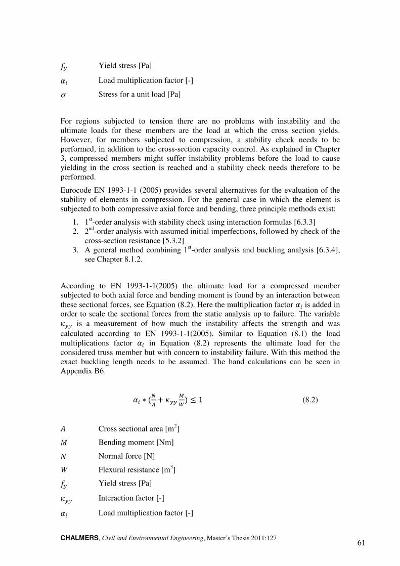
CHALMERS, Civil and Environmental Engineering, Master’s Thesis 2011:127 61
�� Yield stress [Pa]
$' Load multiplication factor [-]
σ Stress for a unit load [Pa]
For regions subjected to tension there are no problems with instability and the ultimate loads for these members are the load at which the cross section yields. However, for members subjected to compression, a stability check needs to be performed, in addition to the cross-section capacity control. As explained in Chapter 3, compressed members might suffer instability problems before the load to cause yielding in the cross section is reached and a stability check needs therefore to be performed.
Eurocode EN 1993-1-1 (2005) provides several alternatives for the evaluation of the stability of elements in compression. For the general case in which the element is subjected to both compressive axial force and bending, three principle methods exist:
1. 1st-order analysis with stability check using interaction formulas [6.3.3] 2. 2nd-order analysis with assumed initial imperfections, followed by check of the
cross-section resistance [5.3.2] 3. A general method combining 1st-order analysis and buckling analysis [6.3.4],
see Chapter 8.1.2.
According to EN 1993-1-1(2005) the ultimate load for a compressed member subjected to both axial force and bending moment is found by an interaction between these sectional forces, see Equation (8.2). Here the multiplication factor $' is added in order to scale the sectional forces from the static analysis up to failure. The variable -�� is a measurement of how much the instability affects the strength and was calculated according to EN 1993-1-1(2005). Similar to Equation (8.1) the load multiplications factor $' in Equation (8.2) represents the ultimate load for the considered truss member but with concern to instability failure. With this method the exact buckling length needs to be assumed. The hand calculations can be seen in Appendix B6.
$' ∗ (=Y + -�� ,�) ≤ 1 (8.2)
� Cross sectional area [m2]
� Bending moment [Nm]
� Normal force [N]
W Flexural resistance [m3]
�� Yield stress [Pa]
-�� Interaction factor [-]
$' Load multiplication factor [-]
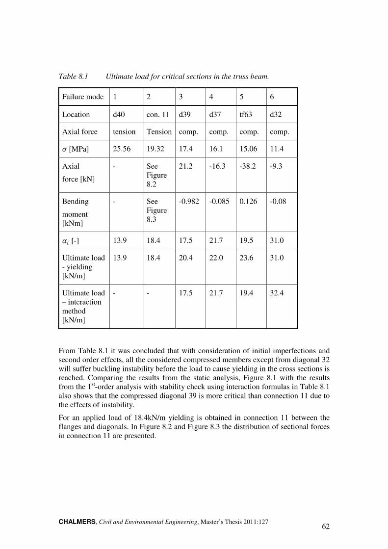
CHALMERS, Civil and Environmental Engineering, Master’s Thesis 2011:127 62
Table 8.1 Ultimate load for critical sections in the truss beam.
Failure mode 1 2 3 4 5 6
Location d40 con. 11 d39 d37 tf63 d32
Axial force tension Tension comp. comp. comp. comp.
� [MPa] 25.56 19.32 17.4 16.1 15.06 11.4
Axial
force [kN]
- See Figure 8.2
21.2 -16.3 -38.2 -9.3
Bending
moment [kNm]
- See Figure 8.3
-0.982 -0.085 0.126 -0.08
$' [-] 13.9 18.4 17.5 21.7 19.5 31.0
Ultimate load - yielding [kN/m]
13.9 18.4 20.4 22.0 23.6 31.0
Ultimate load – interaction method [kN/m]
- - 17.5 21.7 19.4 32.4
From Table 8.1 it was concluded that with consideration of initial imperfections and second order effects, all the considered compressed members except from diagonal 32 will suffer buckling instability before the load to cause yielding in the cross sections is reached. Comparing the results from the static analysis, Figure 8.1 with the results from the 1st-order analysis with stability check using interaction formulas in Table 8.1 also shows that the compressed diagonal 39 is more critical than connection 11 due to the effects of instability.
For an applied load of 18.4kN/m yielding is obtained in connection 11 between the flanges and diagonals. In Figure 8.2 and Figure 8.3 the distribution of sectional forces in connection 11 are presented.
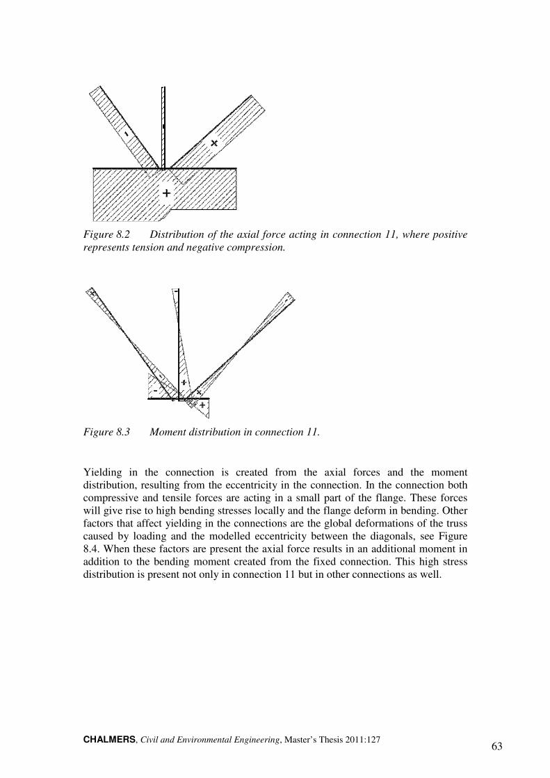
CHALMERS, Civil and Environmental Engineering, Master’s Thesis 2011:127 63
Figure 8.2 Distribution of the axial force acting in connection 11, where positive
represents tension and negative compression.
Figure 8.3 Moment distribution in connection 11.
Yielding in the connection is created from the axial forces and the moment distribution, resulting from the eccentricity in the connection. In the connection both compressive and tensile forces are acting in a small part of the flange. These forces will give rise to high bending stresses locally and the flange deform in bending. Other factors that affect yielding in the connections are the global deformations of the truss caused by loading and the modelled eccentricity between the diagonals, see Figure 8.4. When these factors are present the axial force results in an additional moment in addition to the bending moment created from the fixed connection. This high stress distribution is present not only in connection 11 but in other connections as well.
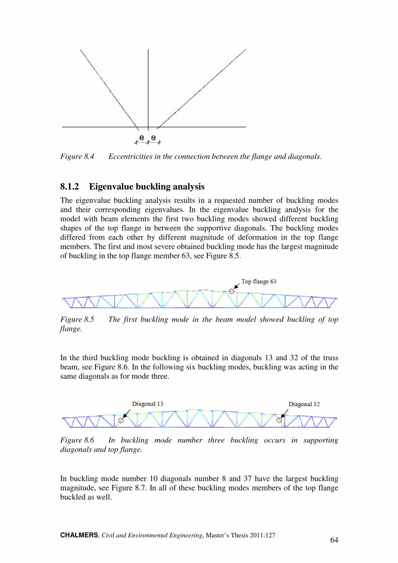
CHALMERS, Civil and Environmental Engineering, Master’s Thesis 2011:127 64
Figure 8.4 Eccentricities in the connection between the flange and diagonals.
8.1.2 Eigenvalue buckling analysis
The eigenvalue buckling analysis results in a requested number of buckling modes and their corresponding eigenvalues. In the eigenvalue buckling analysis for the model with beam elements the first two buckling modes showed different buckling shapes of the top flange in between the supportive diagonals. The buckling modes differed from each other by different magnitude of deformation in the top flange members. The first and most severe obtained buckling mode has the largest magnitude of buckling in the top flange member 63, see Figure 8.5.
Figure 8.5 The first buckling mode in the beam model showed buckling of top
flange.
In the third buckling mode buckling is obtained in diagonals 13 and 32 of the truss beam, see Figure 8.6. In the following six buckling modes, buckling was acting in the same diagonals as for mode three.
Figure 8.6 In buckling mode number three buckling occurs in supporting
diagonals and top flange.
In buckling mode number 10 diagonals number 8 and 37 have the largest buckling magnitude, see Figure 8.7. In all of these buckling modes members of the top flange buckled as well.
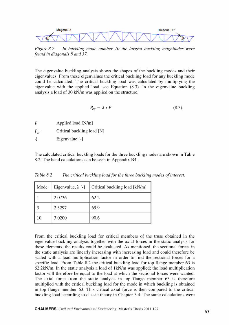
CHALMERS, Civil and Environmental Engineering, Master’s Thesis 2011:127 65
Figure 8.7 In buckling mode number 10 the largest buckling magnitudes were
found in diagonals 8 and 37.
The eigenvalue buckling analysis shows the shapes of the buckling modes and their eigenvalues. From these eigenvalues the critical buckling load for any buckling mode could be calculated. The critical buckling load was calculated by multiplying the eigenvalue with the applied load, see Equation (8.3). In the eigenvalue buckling analysis a load of 30 kN/m was applied on the structure.
�� = λ ∗ � (8.3)
� Applied load [N/m]
�� Critical buckling load [N]
λ Eigenvalue [-]
The calculated critical buckling loads for the three buckling modes are shown in Table 8.2. The hand calculations can be seen in Appendix B4.
Table 8.2 The critical buckling load for the three buckling modes of interest.
Mode Eigenvalue, λ [-] Critical buckling load [kN/m]
1 2.0736 62.2
3 2.3297 69.9
10 3.0200 90.6
From the critical buckling load for critical members of the truss obtained in the eigenvalue buckling analysis together with the axial forces in the static analysis for these elements, the results could be evaluated. As mentioned, the sectional forces in the static analysis are linearly increasing with increasing load and could therefore be scaled with a load multiplication factor in order to find the sectional forces for a specific load. From Table 8.2 the critical buckling load for top flange member 63 is 62.2kN/m. In the static analysis a load of 1kN/m was applied; the load multiplication factor will therefore be equal to the load at which the sectional forces were wanted. The axial force from the static analysis in top flange member 63 is therefore multiplied with the critical buckling load for the mode in which buckling is obtained in top flange member 63. This critical axial force is then compared to the critical buckling load according to classic theory in Chapter 3.4. The same calculations were
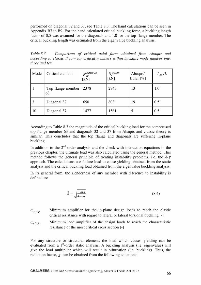
CHALMERS, Civil and Environmental Engineering, Master’s Thesis 2011:127 66
performed on diagonal 32 and 37, see Table 8.3. The hand calculations can be seen in Appendix B7 to B9. For the hand calculated critical buckling force, a buckling length factor of 0,5 was assumed for the diagonals and 1.0 for the top flange member. The critical buckling length was estimated from the eigenvalue buckling analysis.
Table 8.3 Comparison of critical axial force obtained from Abaqus and
according to classic theory for critical members within buckling mode number one,
three and ten.
Mode Critical element ��Y���(� [kN]
���()� [kN]
Abaqus/ Euler [%]
�/
1 Top flange member 63
2378 2743 13 1.0
3 Diagonal 32 650 803 19 0.5
10 Diagonal 37 1477 1561 5 0.5
According to Table 8.3 the magnitude of the critical buckling load for the compressed top flange member 63 and diagonals 32 and 37 from Abaqus and classic theory is similar. This concludes that the top flange and diagonals are suffering in-plane buckling.
In addition to the 2nd-order analysis and the check with interaction equations in the previous chapter, the ultimate load was also calculated using the general method. This method follows the general principle of treating instability problems, i.e. the V-! approach. The calculations use failure load to cause yielding obtained from the static analysis and the critical buckling load obtained from the eigenvalue buckling analysis.
In its general form, the slenderness of any member with reference to instability is defined as:
V̅ = <����,��>?,�� (8.4)
$�,%& Minimum amplifier for the in-plane design loads to reach the elastic critical resistance with regard to lateral or lateral torsional buckling [-]
$()*,+ Minimum load amplifier of the design loads to reach the characteristic resistance of the most critical cross section [-]
For any structure or structural element, the load which causes yielding can be evaluated from a 1st-order static analysis. A buckling analysis (i.e. eigenvalue) will give the load multiplier which will result in bifurcation (i.e. buckling). Thus, the reduction factor, !, can be obtained from the following equations:
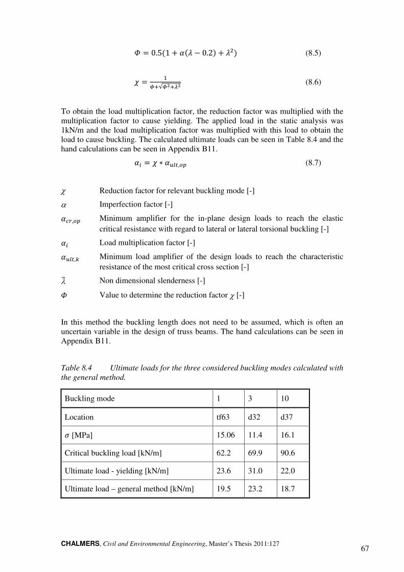
CHALMERS, Civil and Environmental Engineering, Master’s Thesis 2011:127 67
1 = 0.5(1 + $(V − 0.2) + V;) (8.5)
! = kl√kQlnQ (8.6)
To obtain the load multiplication factor, the reduction factor was multiplied with the multiplication factor to cause yielding. The applied load in the static analysis was 1kN/m and the load multiplication factor was multiplied with this load to obtain the load to cause buckling. The calculated ultimate loads can be seen in Table 8.4 and the hand calculations can be seen in Appendix B11.
$' = ! ∗ $()*,%& (8.7)
χ Reduction factor for relevant buckling mode [-]
α Imperfection factor [-]
$�,%& Minimum amplifier for the in-plane design loads to reach the elastic critical resistance with regard to lateral or lateral torsional buckling [-]
$' Load multiplication factor [-]
$()*,+ Minimum load amplifier of the design loads to reach the characteristic resistance of the most critical cross section [-]
λ. Non dimensional slenderness [-]
1 Value to determine the reduction factor χ [-]
In this method the buckling length does not need to be assumed, which is often an uncertain variable in the design of truss beams. The hand calculations can be seen in Appendix B11.
Table 8.4 Ultimate loads for the three considered buckling modes calculated with
the general method.
Buckling mode 1 3 10
Location tf63 d32 d37
� [MPa] 15.06 11.4 16.1
Critical buckling load [kN/m] 62.2 69.9 90.6
Ultimate load - yielding [kN/m] 23.6 31.0 22.0
Ultimate load – general method [kN/m] 19.5 23.2 18.7
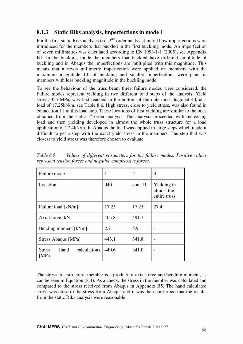
CHALMERS, Civil and Environmental Engineering, Master’s Thesis 2011:127 68
8.1.3 Static Riks analysis, imperfections in mode 1
For the first static Riks analysis (i.e. 2nd-order analysis) initial bow imperfections were introduced for the members that buckled in the first buckling mode. An imperfection of seven millimetres was calculated according to EN 1993-1-1 (2005), see Appendix B1. In the buckling mode the members that buckled have different amplitude of buckling and in Abaqus the imperfections are multiplied with this magnitude. This means that a seven millimetre imperfection were applied on members with the maximum magnitude 1.0 of buckling and smaller imperfections were plant in members with less buckling magnitude in the buckling mode.
To see the behaviour of the truss beam three failure modes were considered, the failure modes represent yielding in two different load steps of the analysis. Yield stress, 355 MPa, was first reached in the bottom of the outermost diagonal 40, at a load of 17.25kN/m, see Table 8.6. High stress, close to yield stress, was also found in connection 11 in this load step. These locations of first yielding are similar to the ones obtained from the static 1st-order analysis. The analysis proceeded with increasing load and then yielding developed in almost the whole truss structure for a load application of 27.4kN/m. In Abaqus the load was applied in large steps which made it difficult to get a step with the exact yield stress in the members. The step that was closest to yield stress was therefore chosen to evaluate.
Table 8.5 Values of different parameters for the failure modes. Positive values
represent tension forces and negative compressive forces.
Failure mode 1 2 3
Location d40 con. 11 Yielding in almost the entire truss
Failure load [kN/m] 17.25 17.25 27.4
Axial force [kN] 405.8 491.7 -
Bending moment [kNm] 2.7 5.9 -
Stress Abaqus [MPa] 443.1 341.8 -
Stress Hand calculations [MPa]
440.6 341.0 -
The stress in a structural member is a product of axial force and bending moment, as can be seen in Equation (8.4). As a check; the stress in the member was calculated and compared to the stress received from Abaqus in Appendix B5. The hand calculated stress was close to the stress from Abaqus and it was then confirmed that the results from the static Riks analysis were reasonable.
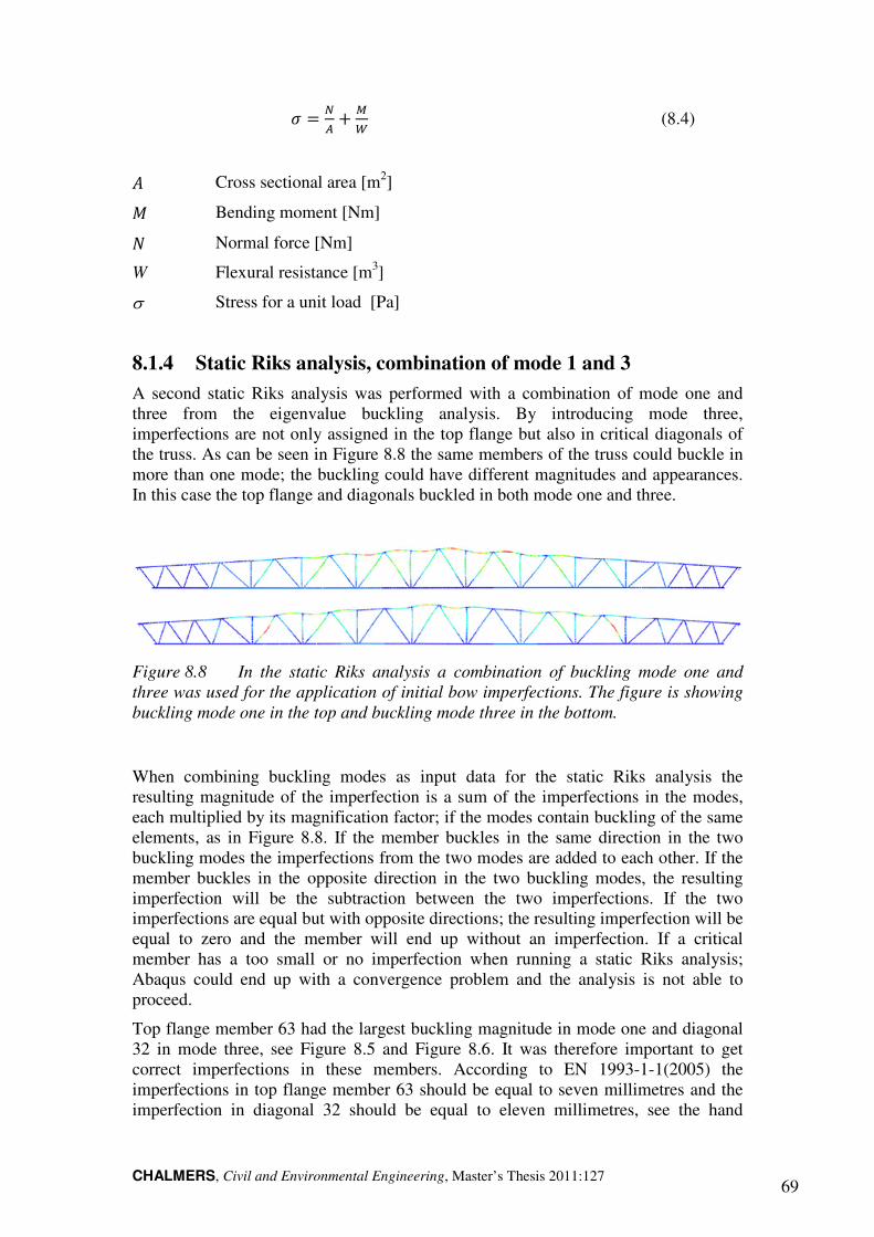
CHALMERS, Civil and Environmental Engineering, Master’s Thesis 2011:127 69
� = =Y + ,
� (8.4)
� Cross sectional area [m2]
� Bending moment [Nm]
� Normal force [Nm]
W Flexural resistance [m3]
σ Stress for a unit load [Pa]
8.1.4 Static Riks analysis, combination of mode 1 and 3
A second static Riks analysis was performed with a combination of mode one and three from the eigenvalue buckling analysis. By introducing mode three, imperfections are not only assigned in the top flange but also in critical diagonals of the truss. As can be seen in Figure 8.8 the same members of the truss could buckle in more than one mode; the buckling could have different magnitudes and appearances. In this case the top flange and diagonals buckled in both mode one and three.
Figure 8.8 In the static Riks analysis a combination of buckling mode one and
three was used for the application of initial bow imperfections. The figure is showing
buckling mode one in the top and buckling mode three in the bottom.
When combining buckling modes as input data for the static Riks analysis the resulting magnitude of the imperfection is a sum of the imperfections in the modes, each multiplied by its magnification factor; if the modes contain buckling of the same elements, as in Figure 8.8. If the member buckles in the same direction in the two buckling modes the imperfections from the two modes are added to each other. If the member buckles in the opposite direction in the two buckling modes, the resulting imperfection will be the subtraction between the two imperfections. If the two imperfections are equal but with opposite directions; the resulting imperfection will be equal to zero and the member will end up without an imperfection. If a critical member has a too small or no imperfection when running a static Riks analysis; Abaqus could end up with a convergence problem and the analysis is not able to proceed.
Top flange member 63 had the largest buckling magnitude in mode one and diagonal 32 in mode three, see Figure 8.5 and Figure 8.6. It was therefore important to get correct imperfections in these members. According to EN 1993-1-1(2005) the imperfections in top flange member 63 should be equal to seven millimetres and the imperfection in diagonal 32 should be equal to eleven millimetres, see the hand
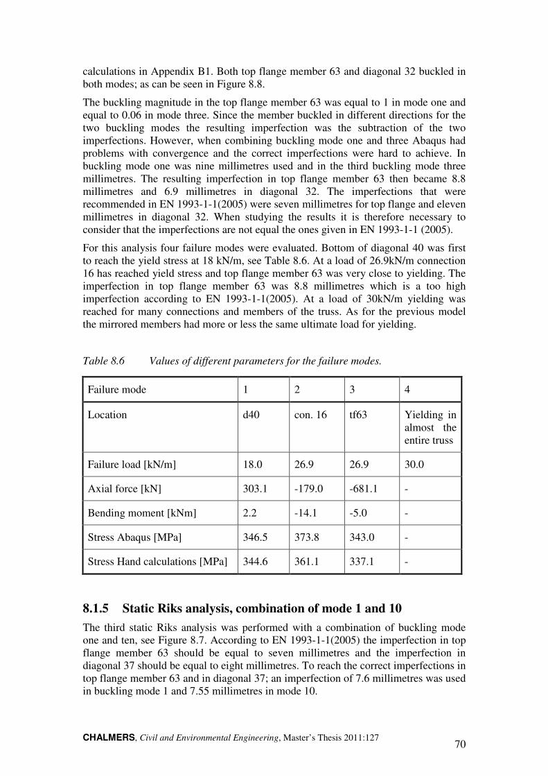
CHALMERS, Civil and Environmental Engineering, Master’s Thesis 2011:127 70
calculations in Appendix B1. Both top flange member 63 and diagonal 32 buckled in both modes; as can be seen in Figure 8.8.
The buckling magnitude in the top flange member 63 was equal to 1 in mode one and equal to 0.06 in mode three. Since the member buckled in different directions for the two buckling modes the resulting imperfection was the subtraction of the two imperfections. However, when combining buckling mode one and three Abaqus had problems with convergence and the correct imperfections were hard to achieve. In buckling mode one was nine millimetres used and in the third buckling mode three millimetres. The resulting imperfection in top flange member 63 then became 8.8 millimetres and 6.9 millimetres in diagonal 32. The imperfections that were recommended in EN 1993-1-1(2005) were seven millimetres for top flange and eleven millimetres in diagonal 32. When studying the results it is therefore necessary to consider that the imperfections are not equal the ones given in EN 1993-1-1 (2005).
For this analysis four failure modes were evaluated. Bottom of diagonal 40 was first to reach the yield stress at 18 kN/m, see Table 8.6. At a load of 26.9kN/m connection 16 has reached yield stress and top flange member 63 was very close to yielding. The imperfection in top flange member 63 was 8.8 millimetres which is a too high imperfection according to EN 1993-1-1(2005). At a load of 30kN/m yielding was reached for many connections and members of the truss. As for the previous model the mirrored members had more or less the same ultimate load for yielding.
Table 8.6 Values of different parameters for the failure modes.
Failure mode 1 2 3 4
Location d40 con. 16 tf63 Yielding in almost the entire truss
Failure load [kN/m] 18.0 26.9 26.9 30.0
Axial force [kN] 303.1 -179.0 -681.1 -
Bending moment [kNm] 2.2 -14.1 -5.0 -
Stress Abaqus [MPa] 346.5 373.8 343.0 -
Stress Hand calculations [MPa] 344.6 361.1 337.1 -
8.1.5 Static Riks analysis, combination of mode 1 and 10
The third static Riks analysis was performed with a combination of buckling mode one and ten, see Figure 8.7. According to EN 1993-1-1(2005) the imperfection in top flange member 63 should be equal to seven millimetres and the imperfection in diagonal 37 should be equal to eight millimetres. To reach the correct imperfections in top flange member 63 and in diagonal 37; an imperfection of 7.6 millimetres was used in buckling mode 1 and 7.55 millimetres in mode 10.

CHALMERS, Civil and Environmental Engineering, Master’s Thesis 2011:127 71
Figure 8.9 In the third static Riks analysis the combination of buckling mode one
and ten was used as the input data for the initial bow imperfections. Buckling mode
one is shown at the top and buckling mode ten at the bottom.
Four failure modes were considered. As for the previous static and static Riks analyses; the first member to reach yielding was diagonal 40 at a load application of 21kN/m, see Table 8.7. The critical diagonal 37 is the second member to reach yielding. Top flange member 65 has an imperfection of 7.8 millimetres; higher than recommended in EN 1993-1-1, caused by having correct imperfections in top flange member 63. The conclusion is that with correct imperfections in top flange member 65 a higher load to cause yielding should be obtained.
Table 8.7 Values of different parameters for the failure modes.
Failure mode 1 2 3 4
Location d40 d37 tf65 tf63
Failure load [kN/m] 21.0 25.4 29.9 34.4
Axial force [kN] 353.9 -285.1 -733.3 -869.1
Bending moment [kNm] 2.6 -2.6 -5.9 -5.1
Stress Abaqus [MPa] 408.3 369.2 380.9 409.9
Stress Hand calculations [MPa] 406.0 366.7 373.3 403.9
8.2 Shell element model
8.2.1 Static analysis
A static analysis was also performed on the model with shell elements. The load was applied as pressure acting on the top face of the both top flanges. A load of 4.167kN/m2 was applied to the beam which corresponds to the load of 1kN/m as used for the beam model.
For the top flange member 63 the ultimate load to cause yielding was calculated to 24.3kN/m based on cross-section resistance, see Equation (8.1). The load calculated according to the general method, explained in the Chapter 8.1.2, was found to be smaller; 20.0kN/m. The hand calculations can be seen in Appendix B10.
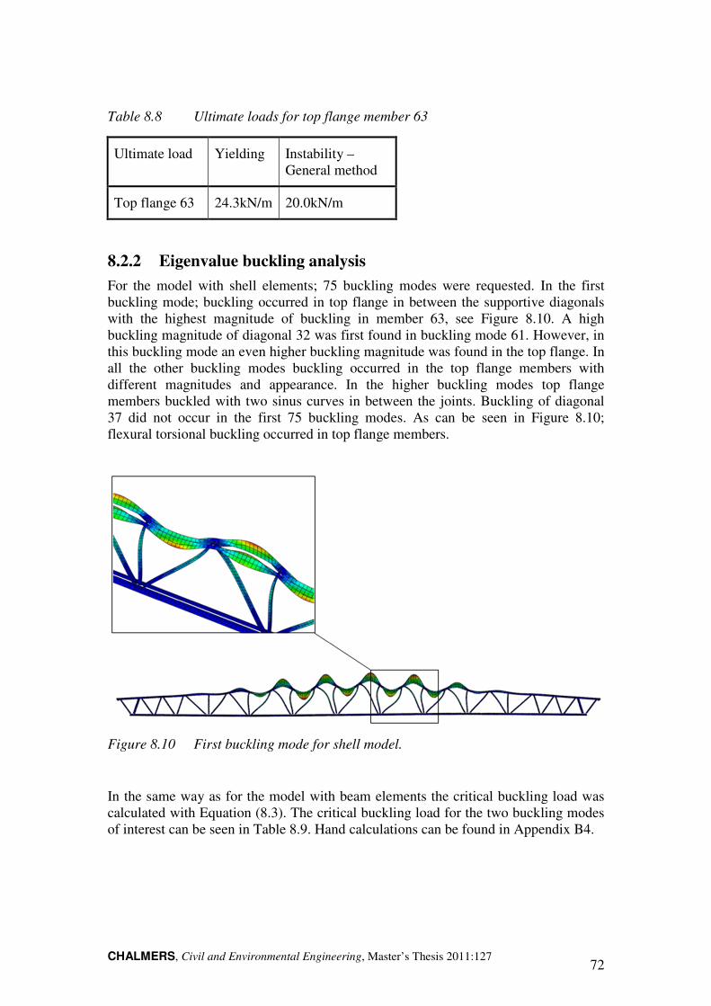
CHALMERS, Civil and Environmental Engineering, Master’s Thesis 2011:127 72
Table 8.8 Ultimate loads for top flange member 63
Ultimate load Yielding Instability – General method
Top flange 63 24.3kN/m 20.0kN/m
8.2.2 Eigenvalue buckling analysis
For the model with shell elements; 75 buckling modes were requested. In the first buckling mode; buckling occurred in top flange in between the supportive diagonals with the highest magnitude of buckling in member 63, see Figure 8.10. A high buckling magnitude of diagonal 32 was first found in buckling mode 61. However, in this buckling mode an even higher buckling magnitude was found in the top flange. In all the other buckling modes buckling occurred in the top flange members with different magnitudes and appearance. In the higher buckling modes top flange members buckled with two sinus curves in between the joints. Buckling of diagonal 37 did not occur in the first 75 buckling modes. As can be seen in Figure 8.10; flexural torsional buckling occurred in top flange members.
Figure 8.10 First buckling mode for shell model.
In the same way as for the model with beam elements the critical buckling load was calculated with Equation (8.3). The critical buckling load for the two buckling modes of interest can be seen in Table 8.9. Hand calculations can be found in Appendix B4.
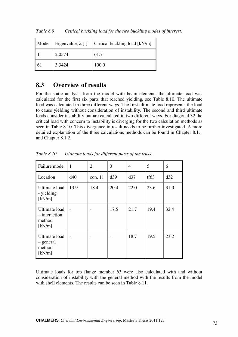
CHALMERS, Civil and Environmental Engineering, Master’s Thesis 2011:127 73
Table 8.9 Critical buckling load for the two buckling modes of interest.
Mode Eigenvalue, λ [-] Critical buckling load [kN/m]
1 2.0574 61.7
61 3.3424 100.0
8.3 Overview of results
For the static analysis from the model with beam elements the ultimate load was calculated for the first six parts that reached yielding, see Table 8.10. The ultimate load was calculated in three different ways. The first ultimate load represents the load to cause yielding without consideration of instability. The second and third ultimate loads consider instability but are calculated in two different ways. For diagonal 32 the critical load with concern to instability is diverging for the two calculation methods as seen in Table 8.10. This divergence in result needs to be further investigated. A more detailed explanation of the three calculations methods can be found in Chapter 8.1.1 and Chapter 8.1.2.
Table 8.10 Ultimate loads for different parts of the truss.
Failure mode 1 2 3 4 5 6
Location d40 con. 11 d39 d37 tf63 d32
Ultimate load - yielding [kN/m]
13.9 18.4 20.4 22.0 23.6 31.0
Ultimate load – interaction method [kN/m]
- - 17.5 21.7 19.4 32.4
Ultimate load – general method [kN/m]
- - - 18.7 19.5 23.2
Ultimate loads for top flange member 63 were also calculated with and without consideration of instability with the general method with the results from the model with shell elements. The results can be seen in Table 8.11.
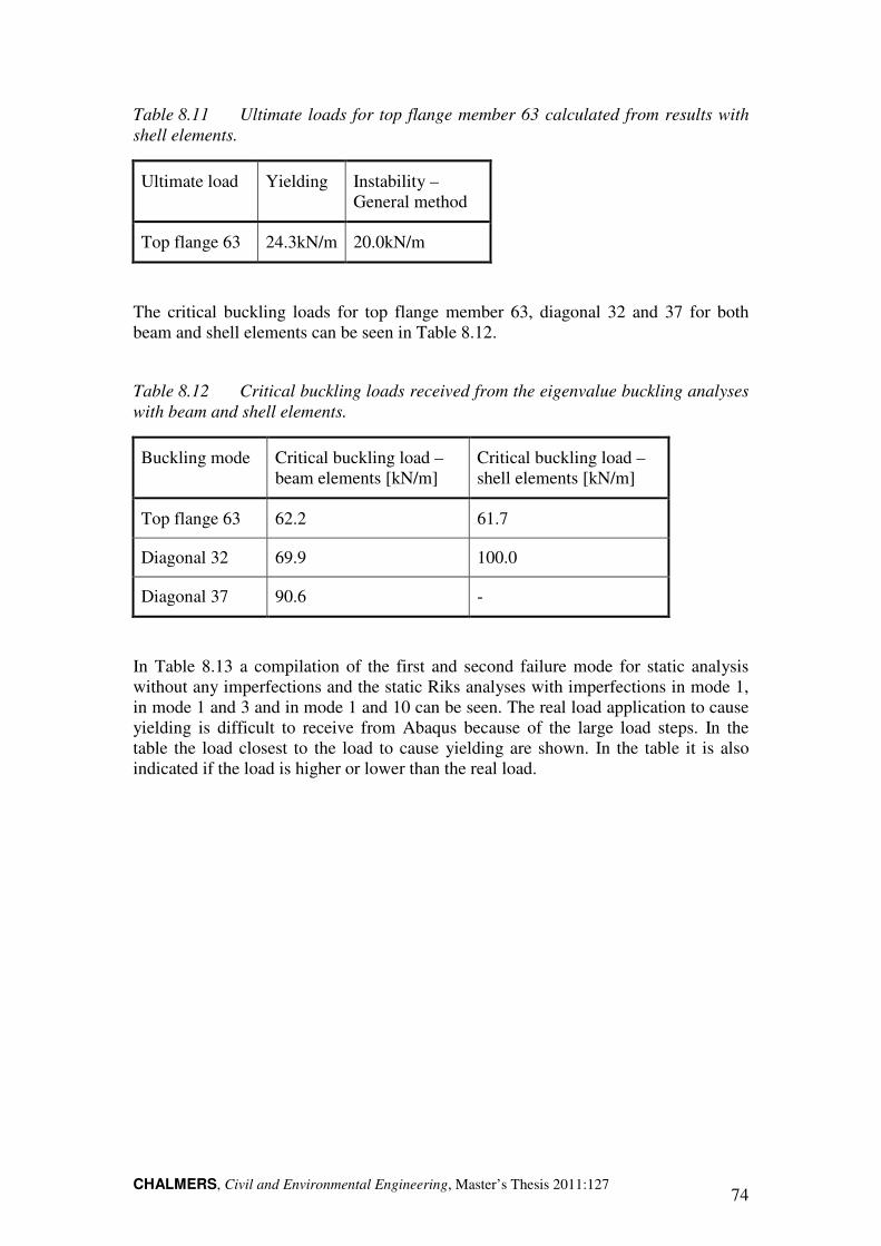
CHALMERS, Civil and Environmental Engineering, Master’s Thesis 2011:127 74
Table 8.11 Ultimate loads for top flange member 63 calculated from results with
shell elements.
Ultimate load Yielding Instability – General method
Top flange 63 24.3kN/m 20.0kN/m
The critical buckling loads for top flange member 63, diagonal 32 and 37 for both beam and shell elements can be seen in Table 8.12.
Table 8.12 Critical buckling loads received from the eigenvalue buckling analyses
with beam and shell elements.
Buckling mode Critical buckling load – beam elements [kN/m]
Critical buckling load – shell elements [kN/m]
Top flange 63 62.2 61.7
Diagonal 32 69.9 100.0
Diagonal 37 90.6 -
In Table 8.13 a compilation of the first and second failure mode for static analysis without any imperfections and the static Riks analyses with imperfections in mode 1, in mode 1 and 3 and in mode 1 and 10 can be seen. The real load application to cause yielding is difficult to receive from Abaqus because of the large load steps. In the table the load closest to the load to cause yielding are shown. In the table it is also indicated if the load is higher or lower than the real load.

CHALMERS, Civil and Environmental Engineering, Master’s Thesis 2011:127 75
Table 8.13 Compilation of the first and second failure mode for the static analysis
and static Riks analyses with imperfections in mode 1, in mode 1 and 3 and in mode 1
and 10.
Static analysis – no imperfections
Imperfections in mode 1
Imperfections in mode 1 and 3
Imperfections in mode 1 and 10
Imperfections in top flange 63
- 7mm 8.8mm 7mm
Imperfections in diagonal 32
- - 7mm -
Imperfections in diagonal 37
- - - 7.55mm
First failure mode
Diagonal 40 Diagonal 40 Diagonal 40 Diagonal 40
Load at first failure mode [kN/m]
13.9 < 17.25 > 18.0 < 21
Second failure mode
Connection 11 Connection 11 Connection 16
Diagonal 37
Load at second failure mode [kN/m]
18.4 > 17.25 < 26.9 < 25.4
CHALMERS, Civil and Environmental Engineering, Master’s Thesis 2011:127 76
9 Discussion
When starting this master thesis the goal was to study truss beams in the Finite Element program Abaqus with consideration of plastic material properties, eccentricities between diagonals within the truss and second order effects due to initial bow imperfections.
The project started with modelling of a pitched truss beam with beam elements as which is generally the most convenient level of modelling in common engineering practice. The aim was thereafter to continue with a more advanced model with shell elements, where a good representation of the welded connection performed at Ranaverken could be included. The results from the beam element model and the model with shell elements was then compared and studied. A large part of the time for this thesis was spent on modelling in Abaqus and the results from the analyses are presented in Chapter 8. Due to convergence problems with the static Riks analyses in Abaqus, the plastic material model was abandoned and elastic second-order analysis was performed, see Chapter 9.6. This implies that an elastic cross-section resistance is adopted, which is valid for some members in the truss. Difficulties and solutions to some of the problems which turned up during this thesis are mentioned in Chapter 7.
9.1 Beam elements
The issue that caused the largest problem was the magnitudes of imperfections when combining two buckling modes. When combining buckling mode one and three the imperfections according to EN 1993-1-1 (2005) was not possible to apply since Abaqus did not complete the analysis due to problem with convergence. The imperfection in the top flange became too large and the imperfection in diagonal 32 too small.
When decreasing the initial bow imperfections in the most critical member of the truss below what is recommended in EN 1993-1-1 (2005) problems with convergence can be obtained in the static Riks analysis. This is believed to be caused by Abaqus not finding equilibrium close to the bifurcation point. As the imperfections are decreased the load to cause buckling in the truss will come closer to the critical load according to classic theory and the behaviour will be similar to a perfect column. When only the first buckling mode was used as an input data the static Riks analysis was completed without problems. When only the third buckling mode was used; the static Riks analysis got convergence problems. The conclusion is therefore that the top flanges are the most critical part of the truss and sensitive to imperfections.
According to the results in Chapter 8.1 the first failure mode for the truss beam was represented by yielding in the tensioned diagonals 5 and 40. This yielding was an important effect of the eccentricities between the diagonals and should therefore be considered in the design of a truss beam. The final failure was reached when yielding started in the compressed members. This yielding was caused by a combination of axial force and second order moment due to deformations. By increasing the imperfections in critical elements the location of first yielding of compressed members was moved, see Chapter 8.1.4 and 8.1.5. This confirms that truss members subjected to tension are not affected by imperfections in the compressed members.

CHALMERS, Civil and Environmental Engineering, Master’s Thesis 2011:127 77
9.2 Comparison of obtained results from the analyses
with beam and shell elements
The ultimate load to cause yielding and the ultimate load with the general method were calculated for the top flange member 63 with both beam and shell elements. The ultimate loads were similar in both models; as can be seen in Table 9.1.
Table 9.1 Comparison between the ultimate load in top flange member 63 for
beam and shell elements.
Ultimate load Yielding Instability with imperfections
Beam 23.6kN/m 19.4N/m
Shell 24.3kN/m 20.0kN/m
The results from the eigenvalue buckling analyses for beam and shell element models showed that the shape and critical buckling load from the first buckling mode are similar. The most critical member of the truss beam is top flange member 63 and the critical buckling loads were 62.2kN/m and 61.7kN/m respectively, see Table 9.2. With beam elements the local twisting of the cross section was not that easy to detect as when modelling with shell elements. As seen in Figure 8.10 flexural torsional buckling was well represented with shell elements but for beam elements it was easy to believe that only in-plane buckling was acting, see Figure 8.8. The first diagonal that buckled was diagonal 32 for both models. However, the critical buckling load for buckling in diagonal 32 was higher with shell elements than with beam elements. Another difference between the two models was that diagonal 37 buckled with beam elements but not with shell elements.
Table 9.2 Comparison of critical buckling loads from beam and shell model.
Buckling mode Critical buckling load – beam elements [kN/m]
Critical buckling load – shell elements [kN/m]
Top flange 63 62.2 61.7
Diagonal 32 69.9 100.0
Diagonal 37 90.6 -
The differences in the results could be explained by that the connections were constructed in different ways for the two models. With beam elements the diagonals were connected to the flanges in one point; the gravity centre of the L profile to the
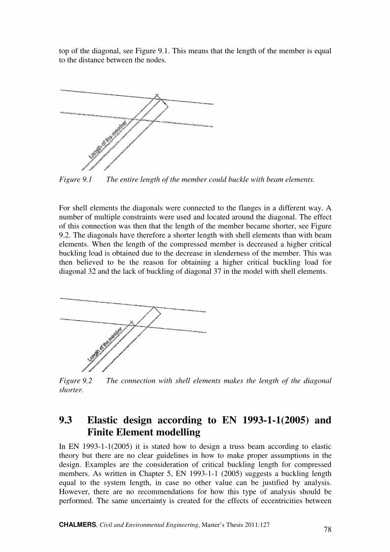
CHALMERS, Civil and Environmental Engineering, Master’s Thesis 2011:127 78
top of the diagonal, see Figure 9.1. This means that the length of the member is equal to the distance between the nodes.
Figure 9.1 The entire length of the member could buckle with beam elements.
For shell elements the diagonals were connected to the flanges in a different way. A number of multiple constraints were used and located around the diagonal. The effect of this connection was then that the length of the member became shorter, see Figure 9.2. The diagonals have therefore a shorter length with shell elements than with beam elements. When the length of the compressed member is decreased a higher critical buckling load is obtained due to the decrease in slenderness of the member. This was then believed to be the reason for obtaining a higher critical buckling load for diagonal 32 and the lack of buckling of diagonal 37 in the model with shell elements.
Figure 9.2 The connection with shell elements makes the length of the diagonal
shorter.
9.3 Elastic design according to EN 1993-1-1(2005) and
Finite Element modelling
In EN 1993-1-1(2005) it is stated how to design a truss beam according to elastic theory but there are no clear guidelines in how to make proper assumptions in the design. Examples are the consideration of critical buckling length for compressed members. As written in Chapter 5, EN 1993-1-1 (2005) suggests a buckling length equal to the system length, in case no other value can be justified by analysis. However, there are no recommendations for how this type of analysis should be performed. The same uncertainty is created for the effects of eccentricities between
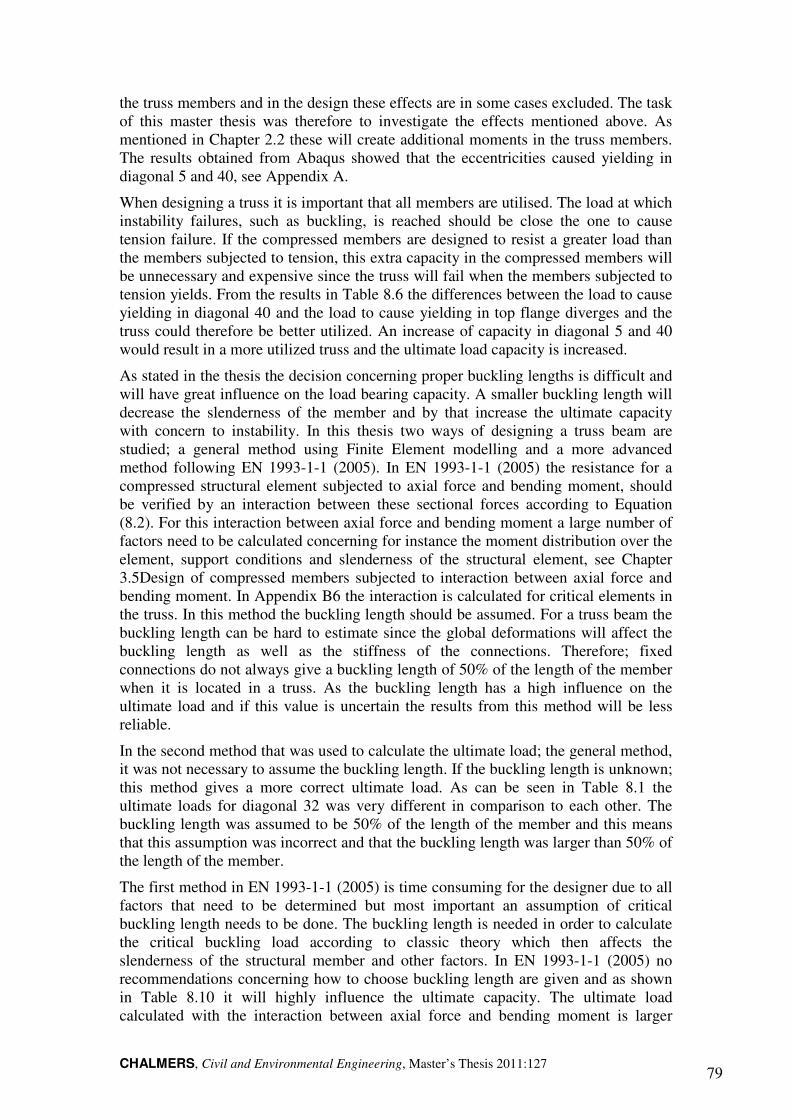
CHALMERS, Civil and Environmental Engineering, Master’s Thesis 2011:127 79
the truss members and in the design these effects are in some cases excluded. The task of this master thesis was therefore to investigate the effects mentioned above. As mentioned in Chapter 2.2 these will create additional moments in the truss members. The results obtained from Abaqus showed that the eccentricities caused yielding in diagonal 5 and 40, see Appendix A.
When designing a truss it is important that all members are utilised. The load at which instability failures, such as buckling, is reached should be close the one to cause tension failure. If the compressed members are designed to resist a greater load than the members subjected to tension, this extra capacity in the compressed members will be unnecessary and expensive since the truss will fail when the members subjected to tension yields. From the results in Table 8.6 the differences between the load to cause yielding in diagonal 40 and the load to cause yielding in top flange diverges and the truss could therefore be better utilized. An increase of capacity in diagonal 5 and 40 would result in a more utilized truss and the ultimate load capacity is increased.
As stated in the thesis the decision concerning proper buckling lengths is difficult and will have great influence on the load bearing capacity. A smaller buckling length will decrease the slenderness of the member and by that increase the ultimate capacity with concern to instability. In this thesis two ways of designing a truss beam are studied; a general method using Finite Element modelling and a more advanced method following EN 1993-1-1 (2005). In EN 1993-1-1 (2005) the resistance for a compressed structural element subjected to axial force and bending moment, should be verified by an interaction between these sectional forces according to Equation (8.2). For this interaction between axial force and bending moment a large number of factors need to be calculated concerning for instance the moment distribution over the element, support conditions and slenderness of the structural element, see Chapter 3.5Design of compressed members subjected to interaction between axial force and bending moment. In Appendix B6 the interaction is calculated for critical elements in the truss. In this method the buckling length should be assumed. For a truss beam the buckling length can be hard to estimate since the global deformations will affect the buckling length as well as the stiffness of the connections. Therefore; fixed connections do not always give a buckling length of 50% of the length of the member when it is located in a truss. As the buckling length has a high influence on the ultimate load and if this value is uncertain the results from this method will be less reliable.
In the second method that was used to calculate the ultimate load; the general method, it was not necessary to assume the buckling length. If the buckling length is unknown; this method gives a more correct ultimate load. As can be seen in Table 8.1 the ultimate loads for diagonal 32 was very different in comparison to each other. The buckling length was assumed to be 50% of the length of the member and this means that this assumption was incorrect and that the buckling length was larger than 50% of the length of the member.
The first method in EN 1993-1-1 (2005) is time consuming for the designer due to all factors that need to be determined but most important an assumption of critical buckling length needs to be done. The buckling length is needed in order to calculate the critical buckling load according to classic theory which then affects the slenderness of the structural member and other factors. In EN 1993-1-1 (2005) no recommendations concerning how to choose buckling length are given and as shown in Table 8.10 it will highly influence the ultimate capacity. The ultimate load calculated with the interaction between axial force and bending moment is larger
CHALMERS, Civil and Environmental Engineering, Master’s Thesis 2011:127 80
compared to the ultimate load found by the general method. Within the interaction a buckling length factor of 0.5 was assumed for the diagonals and as the ultimate load shows to be smaller according to the general method this buckling length factor was too small. This confirms that a stiffness corresponding to a fixed connection between diagonals and flanges is not obtained in the analyses in Abaqus.
Another method to find the ultimate load for a truss beam, described in this thesis and mentioned in EN 1993-1-1 (2005), is to use Finite Element modelling. From this model the ultimate capacity with reference to yielding is found by running a static analysis first. From an eigenvalue buckling analysis, the critical buckling load and the critical truss members with concern to instability is found. With the results from these analyses the slenderness for critical elements could be calculated according to Equation (3.17). In Table 3.2 the buckling curve for the analysed truss member is found and together with the slenderness the reduction factor is found by using Equation (3.15). As described in Chapter 3.4 and Equation (3.13) this reduction factor represents the reduction of the ultimate capacity of the structural element due to instability.
Design with help from Finite Element analysis requires less time for hand calculations and the ultimate capacity is quickly found. However, some knowledge in modelling and time for constructing the model is needed. The advantage with using this kind of modelling is that the ultimate capacity is found without any assumptions considering buckling lengths. From the analyses the designer gains enough information to calculate the ultimate capacity with concern to instability. The fact that no assumptions has to be made by the designer considering stiffness of connections does not only save time for the designer, most important it could prevent instability failures caused by designing for too small buckling lengths.
9.4 Modelling with plastic material
The intention was to model the truss beam with plastic material properties but unfortunately only elastic material properties were possible to include in the static Riks analysis for the truss beam with beam elements. However, elastic material is giving a good representation of the failure modes and general behaviour of the truss.
A column was modelled in order to conclude that the static Riks analysis could include effects of plastic material and initial bow imperfections. As seen in Chapter 4 it is possible to include these effects and at the end of this thesis still no answers were found to why the plastic material could not be included in the truss model. Many trials were made, for example by changing element types, and more of these trials are explained in Chapter 7. If plastic material properties had been included the effects of strain hardening and load redistribution due to yielding in cross sectional parts could have been investigated.
9.5 Modelling with spring connections
In order to evaluate the effects of buckling length and analyse the results obtained from Table 8.10 different types of stiffness’s in the connections were intended to be tested within the truss model. Modelling with fixed connections, by using MPC beam, caused no problems within the beam element analysis and the results are given in
CHALMERS, Civil and Environmental Engineering, Master’s Thesis 2011:127 81
Chapter 8.1. However, in reality constructing a fixed connection between the members of a truss beam with welds is not always feasible.
To compare the two extreme cases with fixed and pinned connections the same truss model was modelled with MPC pin connections. Welds could normally be considered to have a greater stiffness than the one considered for a critical buckling length equal to the system length of the member but the intention was only to see the differences in behaviour for the loaded truss beam. Unfortunately the pinned connections caused instability problems in the analyses. This problem could not be solved even with the help from Abaqus support.
9.6 Further investigations
• To make the correct assumption of the buckling length is difficult for the designer and this issue needs to be further investigated. The influence of buckling lengths for the behaviour and load bearing capacity of the truss could be analysed by introducing different magnitudes of stiffness in the connections. This could be performed by using multiple constraints, MPC pin together with springs with different magnitude of stiffness.
• In order to give recommendations concerning appropriate assumptions in stiffness of welded connections the influence of stiffness has to be analysed as mentioned above. The welds in the connection could also be modelled with its cross sectional area and include plasticity in order to see the response at loading.
• As the results from the analysis with beam elements show that yielding is obtained in the connections between diagonals and flanges the response for compressed members at the point of yielding in the connections could be analysed.
• More studies have to be made in order to find the reason for not reaching convergence when introducing plastic material properties for a large structure such as a truss beam when running a static Riks analysis in Abaqus.
• The effect of eccentricities in the joints needs to further investigated.
CHALMERS, Civil and Environmental Engineering, Master’s Thesis 2011:127 82
10 Conclusions
The conclusions that have been drawn during this master thesis are as follows:
• The behaviour of a truss structure for different stiffness of the connections is possible to analyse by using multiple constrains, MPC pin, together with springs in the three directions X, Y and Z. By changing the stiffness of the springs different buckling lengths of the members are obtained and the effects are seen by running a static Riks analysis.
• By modelling a simply supported column subjected to axial force it was confirmed that the static Riks analysis could include plastic material properties. For the column an initial bow imperfection was introduced from the eigenvalue buckling analysis and together with the second order effects and the plastic material properties convergence was obtained.
• Introducing disturbances as eccentricities and imperfections is possible for a large truss model but together with consideration of plastic material properties convergence problems were obtained.
• From the eigenvalue buckling analysis for beam elements three buckling modes were chosen as the most critical ones, mode one, three and ten in Chapter 8.1. However the results from the static Riks analyses showed that these modes were counteracting each other.
• Imperfections in more than one buckling mode can be included in the analysis but it is important to investigate that they are not counteracting each other such that the critical member ends up with a too high or too low imperfection.
• The most critical truss element in the truss analysed, with concern to buckling instability, is the top flange. Imperfections in other compressed members of the truss did not affect the load bearing capacity. However, first yielding is obtained in diagonals 5 and 40, subjected to tension.
• The eccentricities between truss members caused yielding in connections between diagonals and flanges and the effect in load bearing capacity of the analysed pitched truss needs to be further analysed.
• With shell elements the representation of the connections between diagonals and flanges and the load application are improved.
• If a static analysis is performed on the pitched truss beam the same failure modes are represented as when running the static Riks analysis with imperfections in the critical top flange.
• The differences between ultimate capacity for tension and compression failure in the truss concludes that the truss could be better utilized.
• The consideration of buckling length has a large influence on the ultimate capacity of the pitched truss beam and it is concluded that proper judgements of the stiffness in the connections are hard to make.
• By using Finite Element modelling assumptions regarding buckling lengths are not needed. The risk for instability failures created from wrong assumptions considering this stiffness might therefore be prevented.
CHALMERS, Civil and Environmental Engineering, Master’s Thesis 2011:127 83
11 References
Literature:
Boverket (2011): Erfarenheter från takras i Sverige vintrarna 2009/10 och 2010/11
En slutredovisning av Boverkets regeringsuppdrag M2010/2276/H, Boverket, Karlskrona, Sweden, 11, 18, 21 pp.
EN 1993-1-1 (2005): Eurocode 3: Design of steel structures – Part 1-1: General rules
and rules for buildings. European committee of standardization, Brussels, Belgium, 32-33, 56-58, 69, 82 pp.
EN 1993-1-5 (2006): Eurocode 3: Design of steel structures – Part 1-5: General rules
- Plated structural elements. European committee of standardization, Brussels, Belgium, 64-65, 76-80 pp.
Frühwald, E., Serrano, E., Toratti, T., Emilsson, A. and Thelandersson, S. (2007): Design of safe timber structures – How can we learn from structural failures in
concrete, steel and timber?. Division of Structural Engineering Lund University, Lund, Sweden, 15 pp.
Gozzi, J. (2006): NCCI: Design of roof trusses SN027a-EN-EU. Access steel, Sweden
Höglund, T. (2006): Att konstruera med stål – Modul 6 Stabilitet för balkar och
stänger. SBI - Stålbyggnadsinstitutet, Stockholm, LTU - Luleå tekniska högskola, Luleå, KTH - Kungliga tekniska högskolan, Stockholm, Sweden, 1-6, 9, 11-13, 16, 18, 37-38, 41, 54, 61, 69, 75-76, 79-82 pp.
Johannesson, B., Johansson, G. (1979): Snöskador vintern 1976-1977. Statens råd för byggforskning, R15:1979, Stockholm, Sweden, 41 pp.
Maku (2011): Fackverksbalkar [online] (Updated 2011-07-21) Available at: <http://www.maku.se/> [Accessed 25 March 2010]
Simulia (2010): Abaqus 6.10 Documentation [online] (Updated 2010) Available at: <http://abaqus.civil.uwa.edu.au:2080/v6.10/index.html> [Accessed 24 February 2011]
Sjelvgren, A., Tranvik, P (2010): Slanka knutplåtars inflytande på fackverkets stabilitet. Stålbyggnad, No. 1, 2010, pp. 22-24.
Thomsen, K. (1970): Stålkonstruktioner konstruktionssamlinger. Polyteknisk Forlag, Copenhagen, Denmark, 71 pp.
Thomsen, K. (1971): Stålkonstruktioner gitterdragere. Polyteknisk Forlag, Lyngby, Denmark, 13, 167, 168 pp.
Wredling, S. (1989): Tunga snölaster på tak Norrlands kusttrakter 1987-88. Statens råd för byggforskning, R79:1989, Stockholm, Sweden, 14 pp.
Finite Element programme:
Abaqus, version 6.7.
Abaqus, version 6.8.
Abaqus, version 6.10.
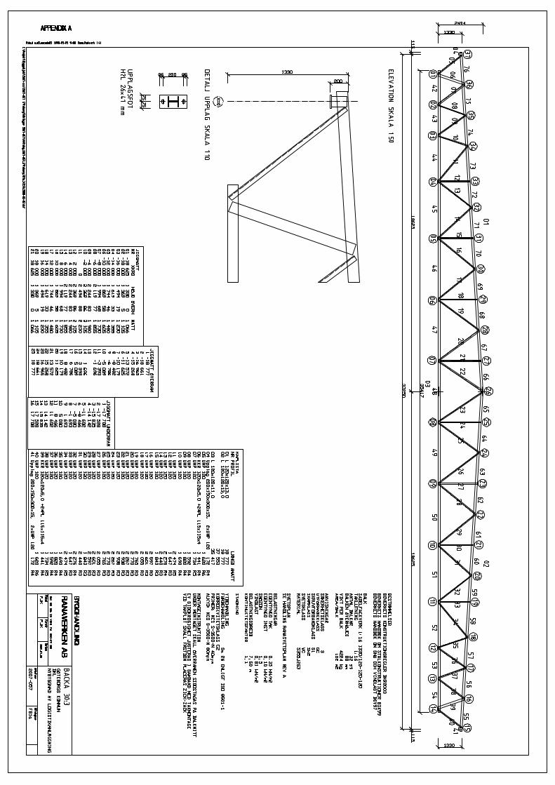

APPENDIX B - Hand calculations
The hand calculations in this thesis is made for checking the accuracy of the models inAbaqus or in some cases used as an input data in Abaqus.
B1. Imperfections
Imperfections are applied to members in the nonlinear analyses. The bucklinganalysis resulted in buckling modes in the top flange and in a diagonal and it is in thismembers imperfections are applied. The imperfections are calculated according toEurocode.
The first thing is to decide the appropriate buckling curve for each memeber. This ismade by look into table 6.2 in EN 1993-1-1. The entire truss beam is made of thesteel class S355. The top flange is constructed by two L profiles and thesecorresponds to the buckling curve b. The diagonal in the other hand is a UNP profilewhich corresponds to the buckling curve c.

The second step is to look into table 5.1 in EN 1993-1-1. The imperfections areused in the Static riks analysis with elastic material properties therefore is the lefthand collumn used in the table.
Imperfections for top flange:
buckb1
2504 10
3−×=:=
The length of the member is measured in the model:
xtf 1.73756m:=
Imperfections used in Abaqus:
i tf xtf buckb⋅ 6.95 103−× m=:=
Imperfections for diagonal 37:
buckc1
2005 10
3−×=:=
The length of the member is measured in the model:
xd 1.615595m:=
Imperfections used in Abaqus:
id xd buckc⋅ 8.078 103−× m=:=
Imperfections for diagonal 32:
buckc1
2005 10
3−×=:=
The length of the member is measured in the model:
xd 2.253098 m:=
Imperfections used in Abaqus:
id xd buckc⋅ 0.011m=:=
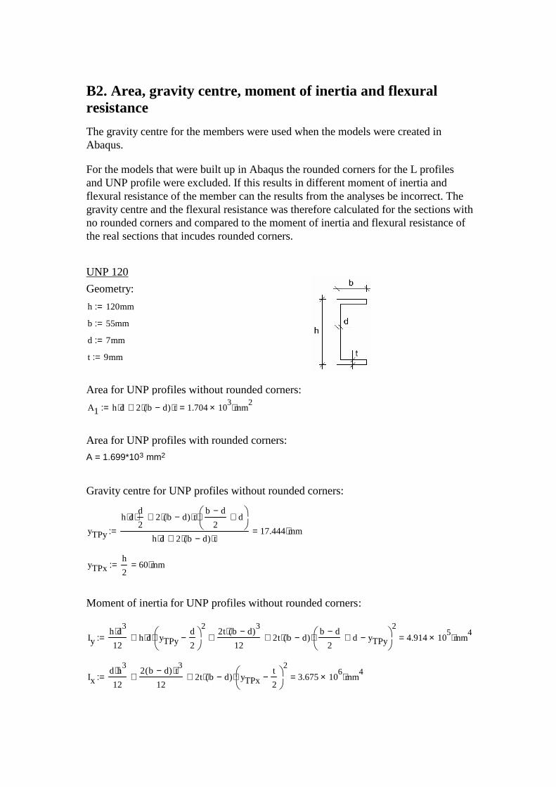
B2. Area, gravity centre, moment of inertia and flexuralresistance
The gravity centre for the members were used when the models were created inAbaqus.
For the models that were built up in Abaqus the rounded corners for the L profilesand UNP profile were excluded. If this results in different moment of inertia andflexural resistance of the member can the results from the analyses be incorrect. Thegravity centre and the flexural resistance was therefore calculated for the sections withno rounded corners and compared to the moment of inertia and flexural resistance ofthe real sections that incudes rounded corners.
UNP 120
Geometry:
h 120mm:=
b 55mm:=
d 7mm:=
t 9mm:=
Area for UNP profiles without rounded corners:
A1 h d⋅ 2 b d−( )⋅ t⋅+ 1.704 103× mm
2⋅=:=
Area for UNP profiles with rounded corners:
A = 1.699*103 mm2
Gravity centre for UNP profiles without rounded corners:
yTPy
h d⋅d
2⋅ 2 b d−( )⋅ t⋅
b d−2
d+
⋅+
h d⋅ 2 b d−( )⋅ t⋅+17.444 mm⋅=:=
yTPxh
260 mm⋅=:=
Moment of inertia for UNP profiles without rounded corners:
Iyh d
3⋅12
h d⋅ yTPyd
2−
2
⋅+2t b d−( )
3⋅12
+ 2t b d−( )⋅b d−
2d+ yTPy−
2
⋅+ 4.914 105× mm
4⋅=:=
Ixd h
3⋅12
2 b d−( ) t3⋅
12+ 2t b d−( )⋅ yTPx
t
2−
2
⋅+ 3.675 106× mm
4⋅=:=
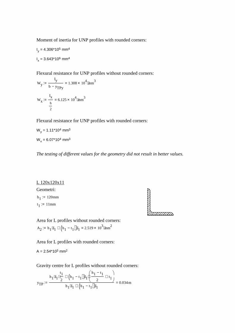
Moment of inertia for UNP profiles with rounded corners:
Iy = 4.306*105 mm4
Ix = 3.643*106 mm4
Flexural resistance for UNP profiles without rounded corners:
Wy
Iy
b yTPy−1.308 10
4× mm3⋅=:=
Wx
Ix
h
2
6.125 104× mm
3⋅=:=
Flexural resistance for UNP profiles with rounded corners:
Wy = 1.11*104 mm3
Wx = 6.07*104 mm3
The testing of different values for the geometry did not result in better values.
L 120x120x11
Geometri:
h1 120mm:=
t1 11mm:=
Area for L profiles without rounded corners:
A2 h1 t1⋅ h1 t1−( ) t1⋅+ 2.519 103× mm
2⋅=:=
Area for L profiles with rounded corners:
A = 2.54*103 mm2
Gravity centre for L profiles without rounded corners:
yTP
h1 t1⋅t1
2⋅ h1 t1−( ) t1⋅
h1 t1−
2t1+
⋅+
h1 t1⋅ h1 t1−( ) t1⋅+0.034m=:=
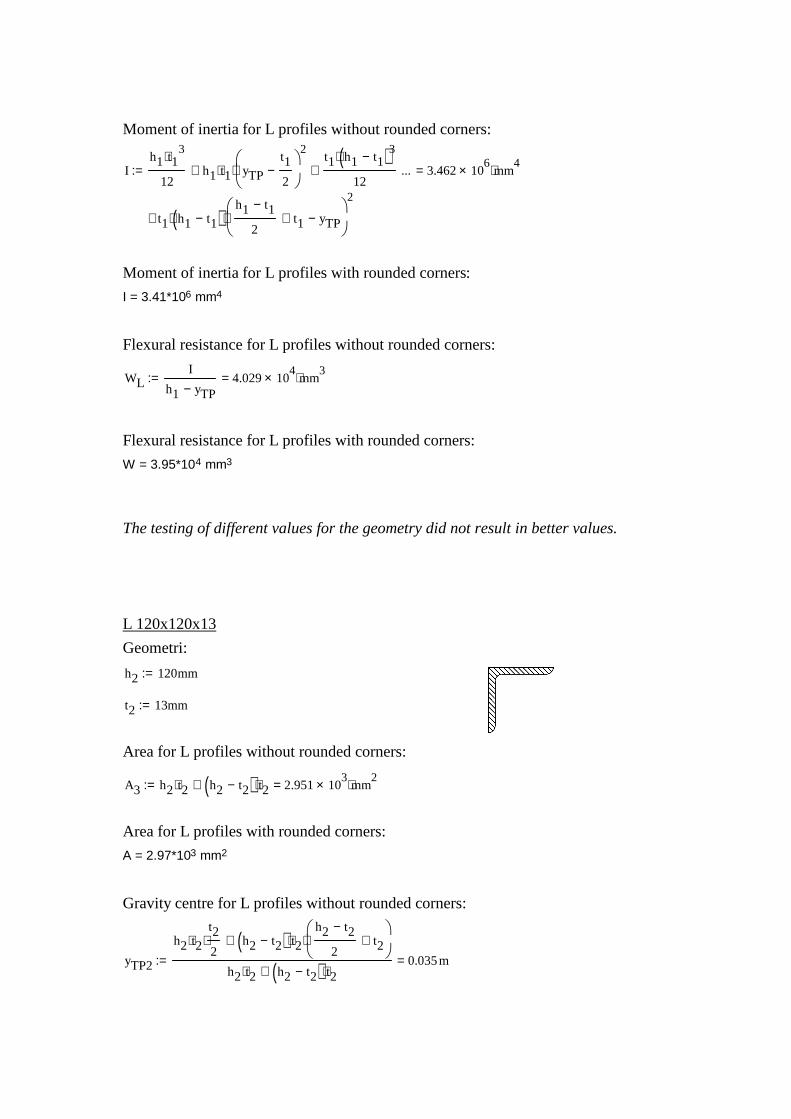
Moment of inertia for L profiles without rounded corners:
Ih1 t1
3⋅
12h1 t1⋅ yTP
t1
2−
2
⋅+t1 h1 t1−( )3⋅
12+
t1 h1 t1−( )⋅h1 t1−
2t1+ yTP−
2
⋅+
... 3.462 106× mm
4⋅=:=
Moment of inertia for L profiles with rounded corners:
I = 3.41*106 mm4
Flexural resistance for L profiles without rounded corners:
WLI
h1 yTP−4.029 10
4× mm3⋅=:=
Flexural resistance for L profiles with rounded corners:
W = 3.95*104 mm3
The testing of different values for the geometry did not result in better values.
L 120x120x13
Geometri:
h2 120mm:=
t2 13mm:=
Area for L profiles without rounded corners:
A3 h2 t2⋅ h2 t2−( ) t2⋅+ 2.951 103× mm
2⋅=:=
Area for L profiles with rounded corners:
A = 2.97*103 mm2
Gravity centre for L profiles without rounded corners:
yTP2
h2 t2⋅t2
2⋅ h2 t2−( ) t2⋅
h2 t2−
2t2+
⋅+
h2 t2⋅ h2 t2−( ) t2⋅+0.035m=:=
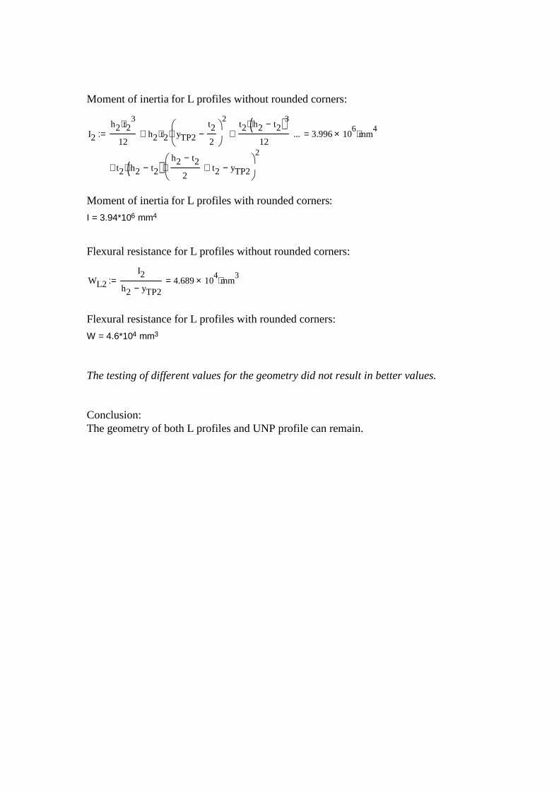
Moment of inertia for L profiles without rounded corners:
I2
h2 t23⋅
12h2 t2⋅ yTP2
t2
2−
2
⋅+t2 h2 t2−( )3⋅
12+
t2 h2 t2−( )⋅h2 t2−
2t2+ yTP2−
2
⋅+
... 3.996 106× mm
4⋅=:=
Moment of inertia for L profiles with rounded corners:
I = 3.94*106 mm4
Flexural resistance for L profiles without rounded corners:
WL2
I2
h2 yTP2−4.689 10
4× mm3⋅=:=
Flexural resistance for L profiles with rounded corners:
W = 4.6*104 mm3
The testing of different values for the geometry did not result in better values.
Conclusion:The geometry of both L profiles and UNP profile can remain.
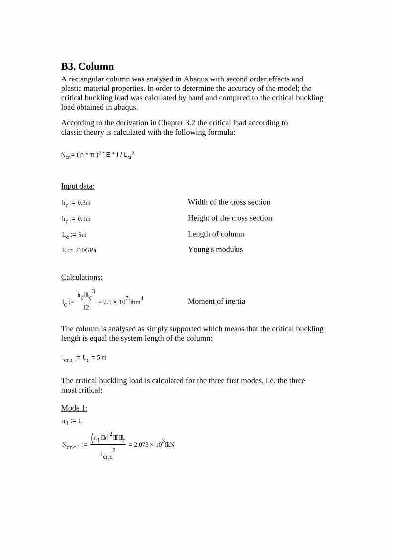
B3. ColumnA rectangular column was analysed in Abaqus with second order effects andplastic material properties. In order to determine the accuracy of the model; thecritical buckling load was calculated by hand and compared to the critical bucklingload obtained in abaqus.
According to the derivation in Chapter 3.2 the critical load according toclassic theory is calculated with the following formula:
Ncr = ( n * π )2 * E * I / Lcr2
Input data:
bc 0.3m:= Width of the cross section
hc 0.1m:= Height of the cross section
Lc 5m:= Length of column
E 210GPa:= Young's modulus
Calculations:
Ic
bc hc3⋅
122.5 10
7× mm4⋅=:= Moment of inertia
The column is analysed as simply supported which means that the critical bucklinglength is equal the system length of the column:
lcr.c Lc 5 m=:=
The critical buckling load is calculated for the three first modes, i.e. the threemost critical:
Mode 1:
n1 1:=
Ncr.c.1
n1 π⋅( )2 E⋅ Ic⋅
lcr.c2
2.073 103× kN⋅=:=

Mode 2:
n2 2:=
Ncr.c.2
n2 π⋅( )2 E⋅ Ic⋅
lcr.c2
8.29 103× kN⋅=:=
Mode 3:
n3 3:=
Ncr.c.3
n3 π⋅( )2 E⋅ Ic⋅
lcr.c2
1.865 104× kN⋅=:=
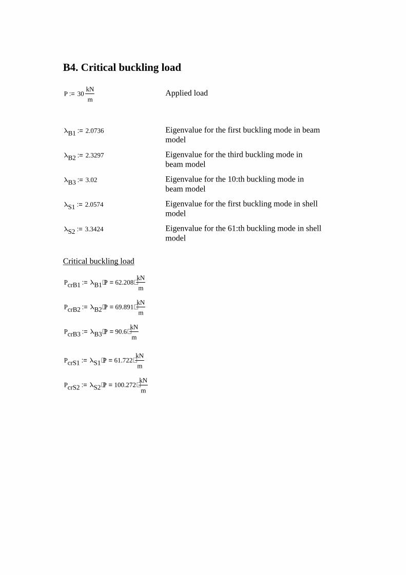
B4. Critical buckling load
P 30kN
m:= Applied load
λB1 2.0736:= Eigenvalue for the first buckling mode in beammodel
λB2 2.3297:= Eigenvalue for the third buckling mode inbeam model
λB3 3.02:= Eigenvalue for the 10:th buckling mode inbeam model
λS1 2.0574:= Eigenvalue for the first buckling mode in shellmodel
λS2 3.3424:= Eigenvalue for the 61:th buckling mode in shellmodel
Critical buckling load
PcrB1 λB1 P⋅ 62.208kN
m⋅=:=
PcrB2 λB2 P⋅ 69.891kN
m⋅=:=
PcrB3 λB3 P⋅ 90.6kN
m⋅=:=
PcrS1 λS1 P⋅ 61.722kN
m⋅=:=
PcrS2 λS2 P⋅ 100.272kN
m⋅=:=
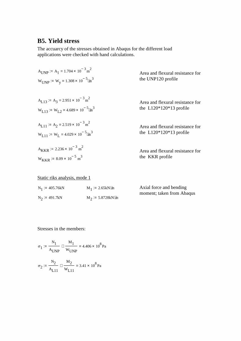
B5. Yield stressThe accuarcy of the stresses obtained in Abaqus for the different loadapplications were checked with hand calculations.
AUNP A1 1.704 103−× m
2=:= Area and flexural resistance forthe UNP120 profileWUNP Wy 1.308 10
5−× m3⋅=:=
AL13 A3 2.951 103−× m
2=:= Area and flexural resistance forthe L120*120*13 profileWL13 WL2 4.689 10
5−× m3⋅=:=
AL11 A2 2.519 103−× m
2=:= Area and flexural resistance forthe L120*120*13 profileWL11 WL 4.029 10
5−× m3⋅=:=
AKKR 2.236 103−× m
2:= Area and flexural resistance forthe KKR profileWKKR 8.09 10
5−× m3:=
Static riks analysis, mode 1
N1 405.76kN:= M1 2.65kN m⋅:= Axial force and bendingmoment; taken from Abaqus
N2 491.7kN:= M2 5.8728kN m⋅:=
Stresses in the members:
σ1
N1
AUNP
M1
WUNP+ 4.406 10
8× Pa=:=
σ2
N2
AL11
M2
WL11+ 3.41 10
8× Pa=:=
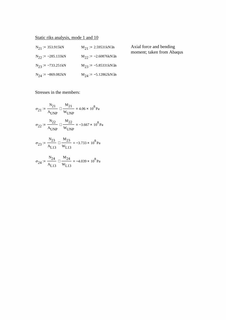
Static riks analysis, mode 1 and 10
N21 353.915kN:= M21 2.59531kN m⋅:= Axial force and bendingmoment; taken from Abaqus
N22 285.133− kN:= M22 2.60876− kN m⋅:=
N23 733.251− kN:= M23 5.85331− kN m⋅:=
N24 869.082− kN:= M24 5.12862− kN m⋅:=
Stresses in the members:
σ21
N21
AUNP
M21
WUNP+ 4.06 10
8× Pa=:=
σ22
N22
AUNP
M22
WUNP+ 3.667− 10
8× Pa=:=
σ23
N23
AL13
M23
WL13+ 3.733− 10
8× Pa=:=
σ24
N24
AL13
M24
WL13+ 4.039− 10
8× Pa=:=

Static riks analysis, mode 1 and 3
N31 303.069kN:= M31 2.18216kN m⋅:= Axial force and bendingmoment; taken from Abaqus
N32 178.985− kN:= M32 14.0903− kN m⋅:=
N33 681.124− kN:= M33 4.98615− kN m⋅:=
N34 542.267− kN:= M34 7.63651− kN m⋅:=
Stresses in the members:
σ31
N31
AUNP
M31
WUNP+ 3.446 10
8× Pa=:=
σ32
N32
AL13
M32
WL13+ 3.611− 10
8× Pa=:=
σ33
N33
AL13
M33
WL13+ 3.371− 10
8× Pa=:=
σ34
N34
AL13
M34
WL13+ 3.466− 10
8× Pa=:=
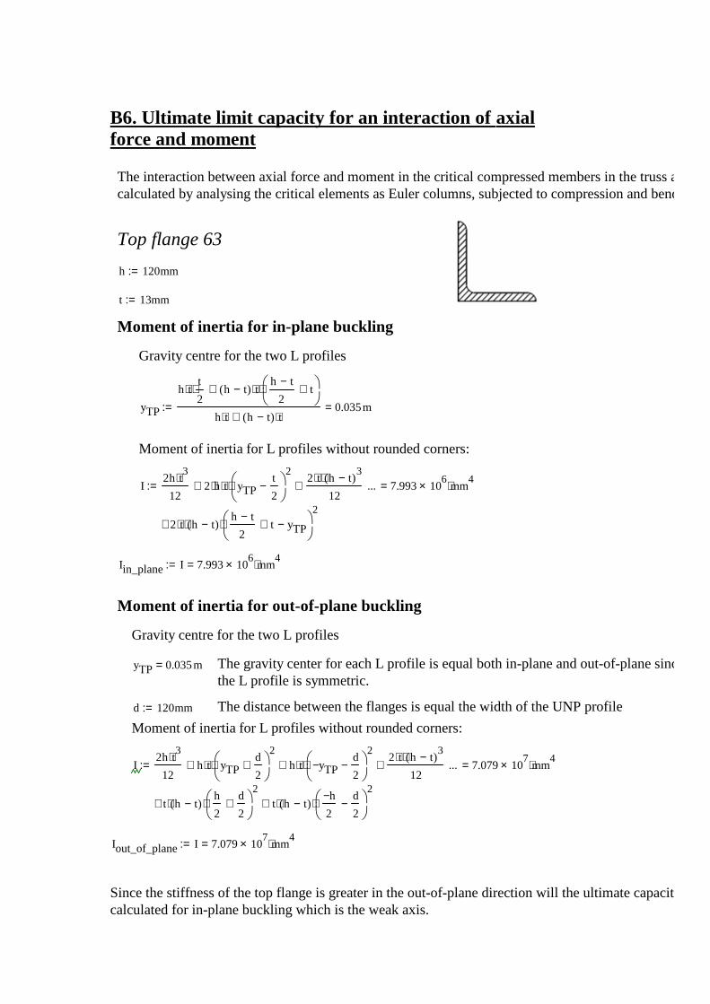
B6. Ultimate limit capacity for an interaction of axialforce and moment
The interaction between axial force and moment in the critical compressed members in the truss arecalculated by analysing the critical elements as Euler columns, subjected to compression and bending.
Top flange 63
h 120mm:=
t 13mm:=
Moment of inertia for in-plane buckling
Gravity centre for the two L profiles
yTP
h t⋅t
2⋅ h t−( ) t⋅
h t−2
t+
⋅+
h t⋅ h t−( ) t⋅+0.035m=:=
Moment of inertia for L profiles without rounded corners:
I2h t
3⋅12
2 h⋅ t⋅ yTPt
2−
2
⋅+2 t⋅ h t−( )
3⋅12
+
2 t⋅ h t−( )⋅h t−
2t+ yTP−
2
⋅+
... 7.993 106× mm
4⋅=:=
Iin_plane I 7.993 106× mm
4⋅=:=
Moment of inertia for out-of-plane buckling
Gravity centre for the two L profiles
yTP 0.035m= The gravity center for each L profile is equal both in-plane and out-of-plane sincethe L profile is symmetric.
d 120mm:= The distance between the flanges is equal the width of the UNP profile
Moment of inertia for L profiles without rounded corners:
I2h t
3⋅12
h t⋅ yTPd
2+
2
⋅+ h t⋅ yTP−d
2−
2
⋅+2 t⋅ h t−( )
3⋅12
+
t h t−( )⋅h
2
d
2+
2
⋅ t h t−( )⋅h−
2
d
2−
2
⋅++
... 7.079 107× mm
4⋅=:=
Iout_of_plane:=Iout_of_plane I 7.079 107× mm
4⋅=:=
Since the stiffness of the top flange is greater in the out-of-plane direction will the ultimate capacity becalculated for in-plane buckling which is the weak axis.

Loads and load effects
qH 0.5kN
m:= Applied load on each L profile in the top flange
NEd 38.2251kN:= Axial force in one of the L profiles for the top flange 63 obtained fromAbaqus
MEd 0.12kN m⋅:= Moment in one of the L profiles for the top flange 63 obtained fromAbaqus
γM1 1.0:=
γM0 1.0:=
Steel S 355
fy 355MPa:= Yield stress
E 210GPa:= Young´s modulus
Stiffness data for one L profile
A 2951mm2:= Cross sectional area
h 0.12 m= Width of flange
b h 0.12 m=:= L profile is symmetric
t 0.013m= Thickness of flange
I 3996 103⋅ mm
4:= Moment of inertia
Wel 46.89 103⋅ mm
3:= Flexural resistance
L 1.73756m:= Length of top flange 63 between the supporting diagonals
Control of cross section class 1993-1-1 [Tabell 5.2]
ε235MPa
fy:=
Flange:
Limit for class 3
h
t15 ε⋅≤ 1=
b h+2t
11.5ε⋅≤ 1=
Flange is in cross section class 3

Moment capacity of one L profile without considerationof instability
1993-1-1 [6.2.5]
Cross section in class 3:
McRd
Wel fy⋅
γM0:=
McRd 16.646 kN m⋅⋅=
McRd MEd> 1=
Compressive capacity of one L profile 1993-1-1 [6.2.4]
NcRd
A fy⋅
γM0:=
NcRd 1.048 103× kN⋅=
NcRd NEd> 1=
Ultimate capacity for one L profile with consideration of instability
Buckling 1993-1-1 [6.3.1]
For columns in cross section class 1, 2 or 3:
NbRd χA fy⋅
γM1⋅=
where χ is a reduction factor for buckling
χ1
Φ Φ2
λ2−+
=
with
Φ 0.5 1 α λ 0.2−( )⋅+ λ2+ ⋅=
The slenderness factor λ:
λNy
Ncr=
A fy⋅
Ncr=
The critical buckling load Ncrπ
2E⋅ I⋅
Lcr2
=
Only buckling in the weak direction is considered
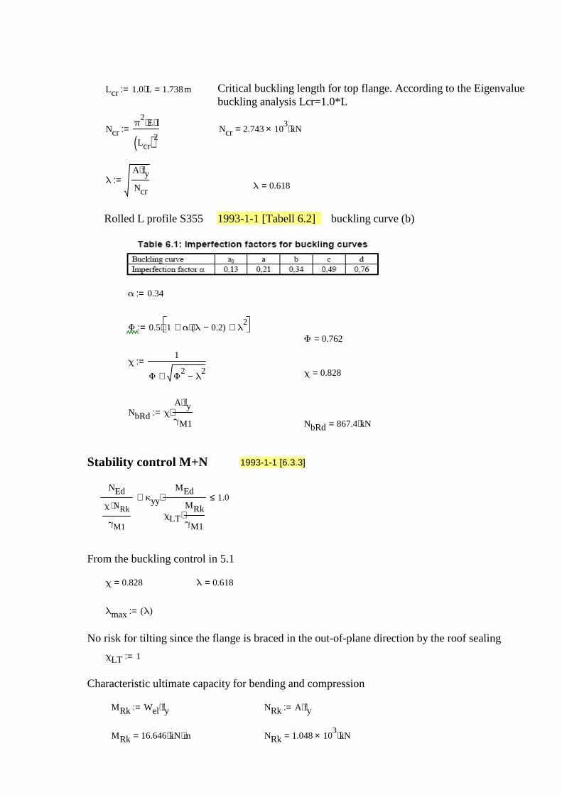
Lcr 1.0 L⋅ 1.738m=:= Critical buckling length for top flange. According to the Eigenvaluebuckling analysis Lcr=1.0*L
Ncrπ
2E⋅ I⋅
Lcr( )2:= Ncr 2.743 10
3× kN⋅=
λA fy⋅
Ncr:=
λ 0.618=
Rolled L profile S355 1993-1-1 [Tabell 6.2] buckling curve (b)
α 0.34:=
Φ 0.5 1 α λ 0.2−( )⋅+ λ2+ ⋅:=
Φ 0.762=
χ1
Φ Φ2
λ2−+
:=χ 0.828=
NbRd χA fy⋅
γM1⋅:=
NbRd 867.4 kN⋅=
Stability control M+N 1993-1-1 [6.3.3]
NEd
χ NRk⋅
γM1
κyy
MEd
χLT
MRk
γM1⋅
⋅+ 1.0≤
From the buckling control in 5.1
χ 0.828= λ 0.618=
λmax λ( ):=
No risk for tilting since the flange is braced in the out-of-plane direction by the roof sealing
χLT 1:=
Characteristic ultimate capacity for bending and compression
MRk Wel fy⋅:= NRk A fy⋅:=
MRk 16.646 kN m⋅⋅= NRk 1.048 103× kN⋅=
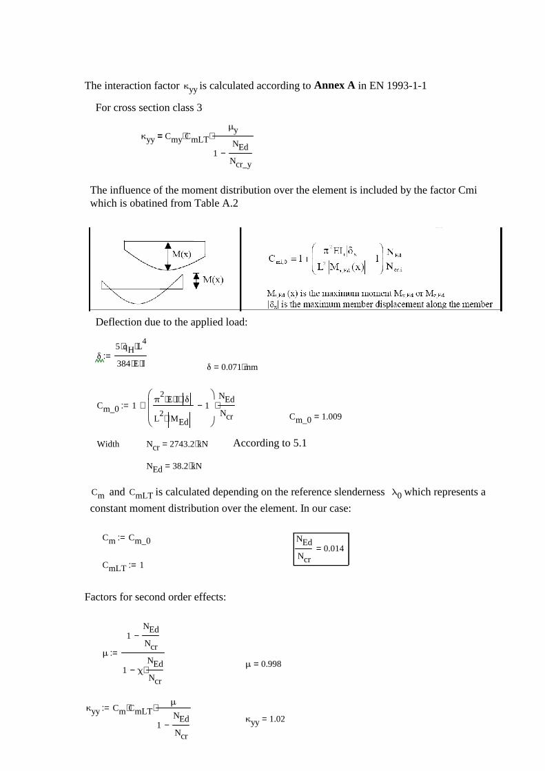
The interaction factor κyy is calculated according to Annex A in EN 1993-1-1
For cross section class 3
κyy Cmy CmLT⋅μy
1NEd
Ncr_y−
⋅=
The influence of the moment distribution over the element is included by the factor Cmiwhich is obatined from Table A.2
Deflection due to the applied load:
δ5 qH⋅ L
4⋅
384 E⋅ I⋅:=
δ 0.071 mm⋅=
Cm_0 1π
2E⋅ I⋅ δ⋅
L2
MEd⋅1−
NEd
Ncr⋅+:=
Cm_0 1.009=
Width Ncr 2743.2 kN⋅= According to 5.1
NEd 38.2 kN⋅=
Cm and CmLT is calculated depending on the reference slenderness λ0 which represents a
constant moment distribution over the element. In our case:
Cm Cm_0:= NEd
Ncr0.014=
CmLT 1:=
Factors for second order effects:
μ
1NEd
Ncr−
1 χNEd
Ncr⋅−
:=μ 0.998=
κyy Cm CmLT⋅μ
1NEd
Ncr−
⋅:=κyy 1.02=
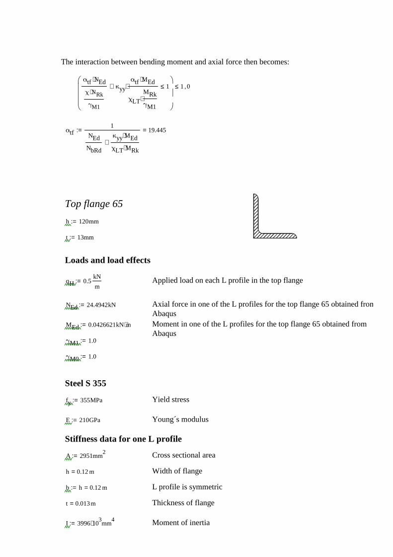
The interaction between bending moment and axial force then becomes:
αtf NEd⋅
χ NRk⋅
γM1
κyy
αtf MEd⋅
χLT
MRk
γM1⋅
⋅+ 1≤
1≤ 0,
αtf1
NEd
NbRd
κyy MEd⋅
χLT MRk⋅+
19.445=:=
Top flange 65
h 120mm:=
t 13mm:=
Loads and load effects
qH 0.5kN
m:= Applied load on each L profile in the top flange
NEd 24.4942kN:= Axial force in one of the L profiles for the top flange 65 obtained fromAbaqus
MEd 0.0426621kN m⋅:= Moment in one of the L profiles for the top flange 65 obtained fromAbaqus
γM1 1.0:=
γM0 1.0:=
Steel S 355
fy 355MPa:= Yield stress
E 210GPa:= Young´s modulus
Stiffness data for one L profile
A 2951mm2:= Cross sectional area
h 0.12 m= Width of flange
b h 0.12 m=:= L profile is symmetric
t 0.013m= Thickness of flange
I 3996 103⋅ mm
4:= Moment of inertia
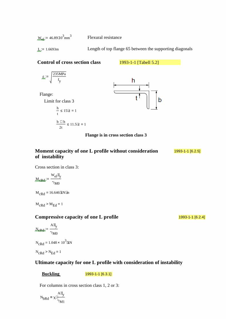
Wel 46.89 103⋅ mm
3:= Flexural resistance
L 1.6693m:= Length of top flange 65 between the supporting diagonals
Control of cross section class 1993-1-1 [Tabell 5.2]
ε235MPa
fy:=
Flange:
Limit for class 3
h
t15 ε⋅≤ 1=
b h+2t
11.5ε⋅≤ 1=
Flange is in cross section class 3
Moment capacity of one L profile without considerationof instability
1993-1-1 [6.2.5]
Cross section in class 3:
McRd
Wel fy⋅
γM0:=
McRd 16.646 kN m⋅⋅=
McRd MEd> 1=
Compressive capacity of one L profile 1993-1-1 [6.2.4]
NcRd
A fy⋅
γM0:=
NcRd 1.048 103× kN⋅=
NcRd NEd> 1=
Ultimate capacity for one L profile with consideration of instability
Buckling 1993-1-1 [6.3.1]
For columns in cross section class 1, 2 or 3:
NbRd χA fy⋅
γM1⋅=
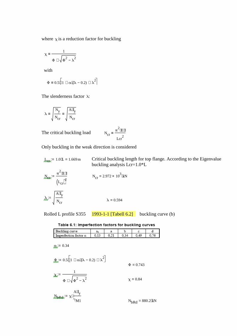
where χ is a reduction factor for buckling
χ1
Φ Φ2
λ2−+
=
with
Φ 0.5 1 α λ 0.2−( )⋅+ λ2+ ⋅=
The slenderness factor λ:
λNy
Ncr=
A fy⋅
Ncr=
The critical buckling load Ncrπ
2E⋅ I⋅
Lcr2
=
Only buckling in the weak direction is considered
Lcr 1.0 L⋅ 1.669m=:= Critical buckling length for top flange. According to the Eigenvaluebuckling analysis Lcr=1.0*L
Ncrπ
2E⋅ I⋅
Lcr( )2:= Ncr 2.972 10
3× kN⋅=
λA fy⋅
Ncr:=
λ 0.594=
Rolled L profile S355 1993-1-1 [Tabell 6.2] buckling curve (b)
α 0.34:=
Φ 0.5 1 α λ 0.2−( )⋅+ λ2+ ⋅:=
Φ 0.743=
χ1
Φ Φ2
λ2−+
:=χ 0.84=
NbRd χA fy⋅
γM1⋅:=
NbRd 880.2 kN⋅=
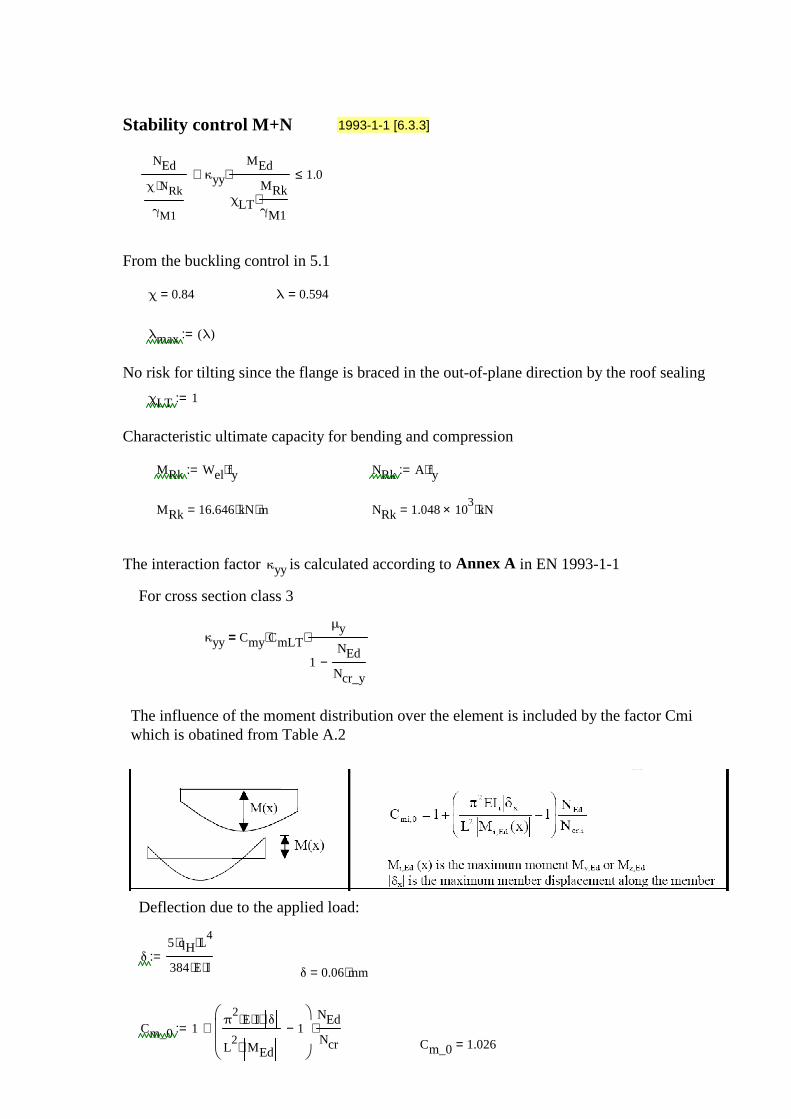
Stability control M+N 1993-1-1 [6.3.3]
NEd
χ NRk⋅
γM1
κyy
MEd
χLT
MRk
γM1⋅
⋅+ 1.0≤
From the buckling control in 5.1
χ 0.84= λ 0.594=
λmax λ( ):=
No risk for tilting since the flange is braced in the out-of-plane direction by the roof sealing
χLT 1:=
Characteristic ultimate capacity for bending and compression
MRk Wel fy⋅:= NRk A fy⋅:=
MRk 16.646 kN m⋅⋅= NRk 1.048 103× kN⋅=
The interaction factor κyy is calculated according to Annex A in EN 1993-1-1
For cross section class 3
κyy Cmy CmLT⋅μy
1NEd
Ncr_y−
⋅=
The influence of the moment distribution over the element is included by the factor Cmiwhich is obatined from Table A.2
Deflection due to the applied load:
δ5 qH⋅ L
4⋅
384 E⋅ I⋅:=
δ 0.06 mm⋅=
Cm_0 1π
2E⋅ I⋅ δ⋅
L2
MEd⋅1−
NEd
Ncr⋅+:=
Cm_0 1.026=
Width Ncr 2972.2 kN⋅= According to 5.1
NEd 24.5 kN⋅=
Cm and CmLT is calculated depending on the reference slenderness λ0 which represents a
constant moment distribution over the element. In our case:
Cm Cm_0:= NEd
Ncr8.241 10
3−×=
CmLT 1:=
Factors for second order effects:
μ
1NEd
Ncr−
1 χNEd
Ncr⋅−
:=μ 0.999=
κyy Cm CmLT⋅μ
1NEd
Ncr−
⋅:=κyy 1.034=
The interaction between bending moment and axial force then becomes:
αtf NEd⋅
χ NRk⋅
γM1
κyy
αtf MEd⋅
χLT
MRk
γM1⋅
⋅+ 1≤
1≤ 0,
αtf1
NEd
NbRd
κyy MEd⋅
χLT MRk⋅+
32.812=:=
Diagonal 37
h 120mm:=
b 55mm:=
d 7mm:=
t 9mm:=
Moment of inertia for in-plane buckling
yTP
h d⋅d
2⋅ 2 b d−( )⋅ t⋅
b d−2
d+
⋅+
h d⋅ 2 b d−( )⋅ t⋅+17.444 mm⋅=:=
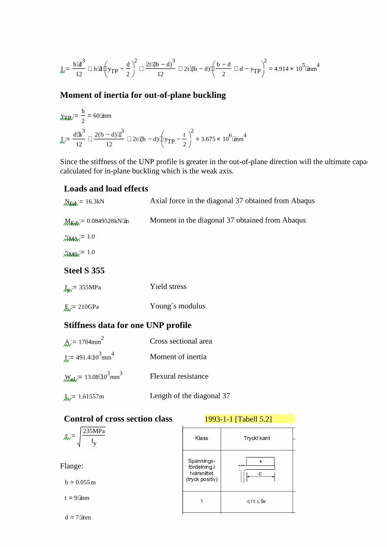
Ih d
3⋅12
h d⋅ yTPd
2−
2
⋅+2t b d−( )
3⋅12
+ 2t b d−( )⋅b d−
2d+ yTP−
2
⋅+ 4.914 105× mm
4⋅=:=
Moment of inertia for out-of-plane buckling
yTPh
260 mm⋅=:=
Id h
3⋅12
2 b d−( ) t3⋅
12+ 2t b d−( )⋅ yTP
t
2−
2
⋅+ 3.675 106× mm
4⋅=:=
Since the stiffness of the UNP profile is greater in the out-of-plane direction will the ultimate capacity becalculated for in-plane buckling which is the weak axis.
Loads and load effectsNEd 16.3kN:= Axial force in the diagonal 37 obtained from Abaqus
MEd 0.0849528kN m⋅:= Moment in the diagonal 37 obtained from Abaqus
γM1 1.0:=
γM0 1.0:=
Steel S 355
fy 355MPa:= Yield stress
E 210GPa:= Young´s modulus
Stiffness data for one UNP profile
A 1704mm2:= Cross sectional area
I 491.4 103⋅ mm
4:= Moment of inertia
Wel 13.08 103⋅ mm
3:= Flexural resistance
L 1.61557m:= Length of the diagonal 37
Control of cross section class 1993-1-1 [Tabell 5.2]
ε235MPa
fy:=
Flange:
b 0.055m=
t 9 mm⋅=
d 7 mm⋅=
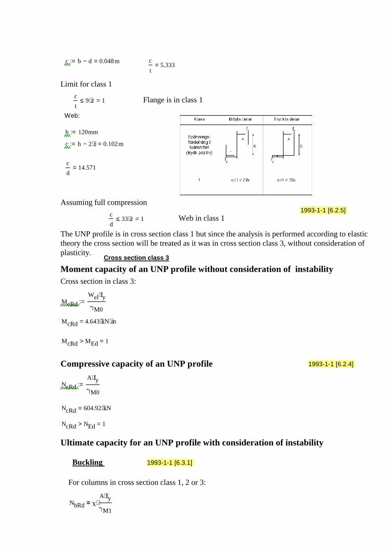
c b d− 0.048m=:= c
t5.333=
Limit for class 1
c
t9 ε⋅≤ 1= Flange is in class 1
Web:
h 120mm:=
c h 2 t⋅− 0.102m=:=
c
d14.571=
Assuming full compression1993-1-1 [6.2.5]
c
d33 ε⋅≤ 1= Web in class 1
The UNP profile is in cross section class 1 but since the analysis is performed according to elastictheory the cross section will be treated as it was in cross section class 3, without consideration ofplasticity.
Cross section class 3
Moment capacity of an UNP profile without consideration of instabilityCross section in class 3:
McRd
Wel fy⋅
γM0:=
McRd 4.643 kN m⋅⋅=
McRd MEd> 1=
Compressive capacity of an UNP profile 1993-1-1 [6.2.4]
NcRd
A fy⋅
γM0:=
NcRd 604.92 kN⋅=
NcRd NEd> 1=
Ultimate capacity for an UNP profile with consideration of instability
Buckling 1993-1-1 [6.3.1]
For columns in cross section class 1, 2 or 3:
NbRd χA fy⋅
γM1⋅=
where is a reduction factor for buckling
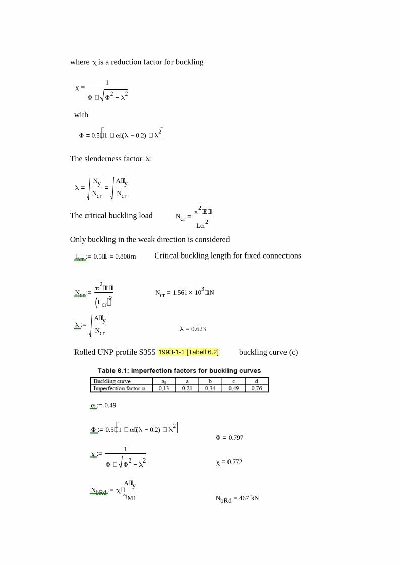
where χ is a reduction factor for buckling
χ1
Φ Φ2
λ2−+
=
with
Φ 0.5 1 α λ 0.2−( )⋅+ λ2+ ⋅=
The slenderness factor λ:
λNy
Ncr=
A fy⋅
Ncr=
The critical buckling load Ncrπ
2E⋅ I⋅
Lcr2
=
Only buckling in the weak direction is considered
Lcr 0.5 L⋅ 0.808m=:= Critical buckling length for fixed connections
Ncrπ
2E⋅ I⋅
Lcr( )2:= Ncr 1.561 10
3× kN⋅=
λA fy⋅
Ncr:=
λ 0.623=
Rolled UNP profile S355 1993-1-1 [Tabell 6.2] buckling curve (c)
α 0.49:=
Φ 0.5 1 α λ 0.2−( )⋅+ λ2+ ⋅:=
Φ 0.797=
χ1
Φ Φ2
λ2−+
:=χ 0.772=
NbRd χA fy⋅
γM1⋅:=
NbRd 467 kN⋅=
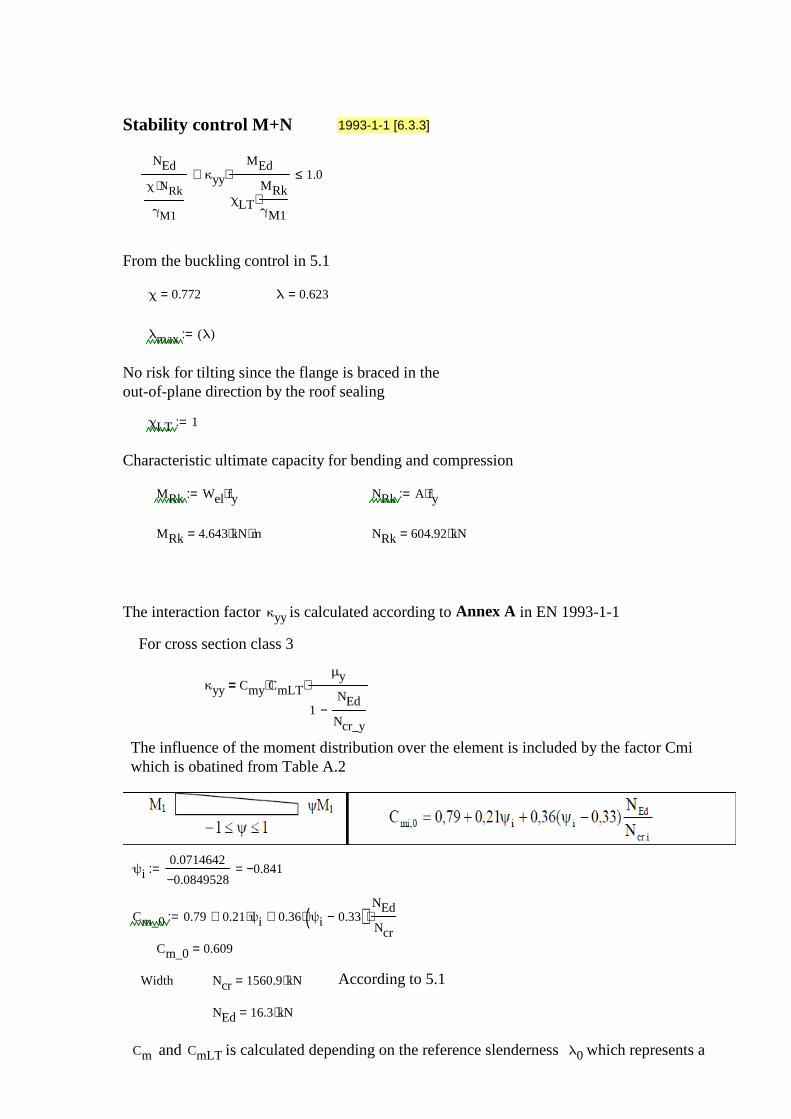
Stability control M+N 1993-1-1 [6.3.3]
NEd
χ NRk⋅
γM1
κyy
MEd
χLT
MRk
γM1⋅
⋅+ 1.0≤
From the buckling control in 5.1
χ 0.772= λ 0.623=
λmax λ( ):=
No risk for tilting since the flange is braced in theout-of-plane direction by the roof sealing
χLT 1:=
Characteristic ultimate capacity for bending and compression
MRk Wel fy⋅:= NRk A fy⋅:=
MRk 4.643 kN m⋅⋅= NRk 604.92 kN⋅=
The interaction factor κyy is calculated according to Annex A in EN 1993-1-1
For cross section class 3
κyy Cmy CmLT⋅μy
1NEd
Ncr_y−
⋅=
The influence of the moment distribution over the element is included by the factor Cmiwhich is obatined from Table A.2
ψi0.0714642
0.0849528−0.841−=:=
Cm_0 0.79 0.21ψi⋅+ 0.36 ψi 0.33−( )⋅NEd
Ncr⋅+:=
Cm_0 0.609=
Width Ncr 1560.9 kN⋅= According to 5.1
NEd 16.3 kN⋅=
Cm and CmLT is calculated depending on the reference slenderness λ0 which represents a
constant moment distribution over the element. In our case:

constant moment distribution over the element. In our case:
Cm Cm_0:=
CmLT 1:=
Factors for second order effects:
μ
1NEd
Ncr−
1 χNEd
Ncr⋅−
:=
μ 0.998=
κyy Cm CmLT⋅μ
1NEd
Ncr−
⋅:=
κyy 0.614=
The interaction between bending moment and axial force then becomes:
αtf NEd⋅
χ NRk⋅
γM1
κyy
αtf MEd⋅
χLT
MRk
γM1⋅
⋅+ 1≤
1≤ 0,
αtf1
NEd
NbRd
κyy MEd⋅
χLT MRk⋅+
21.674=:=
Diagonal 39
h 120mm:=
b 120mm:=
d 5mm:=
t 5mm:=
Loads and load effectsNEd 21.23kN:= Axial force in diagonal 39 obtained from Abaqus
MEd 0.9816kN m⋅:= Moment in diagonal 39 obtained from Abaqus
γM1 1.0:=
γM0 1.0:=
Steel S 355
fy 355MPa:= Yield stress
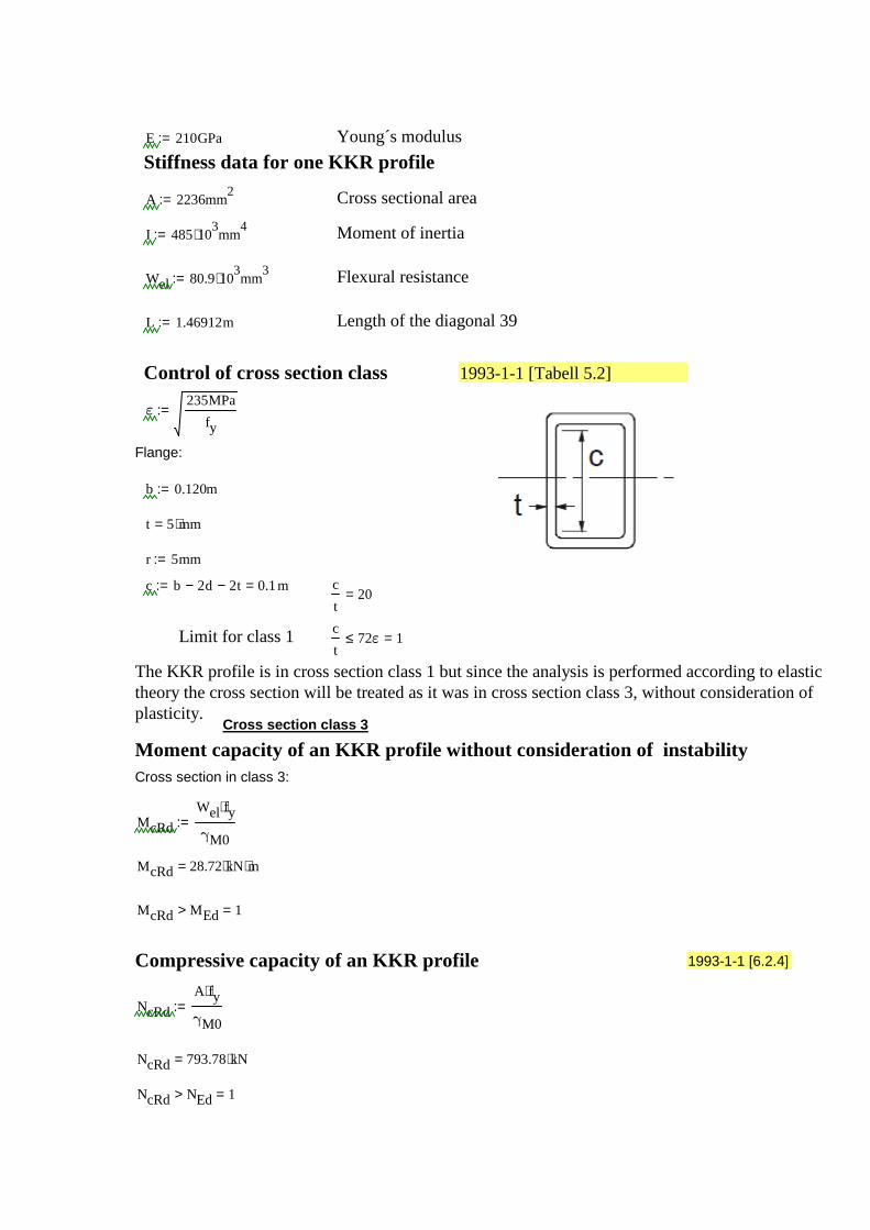
E 210GPa:= Young´s modulus
Stiffness data for one KKR profile
A 2236mm2:= Cross sectional area
I 485 103⋅ mm
4:= Moment of inertia
Wel 80.9 103⋅ mm
3:= Flexural resistance
L 1.46912m:= Length of the diagonal 39
Control of cross section class 1993-1-1 [Tabell 5.2]
ε235MPa
fy:=
Flange:
b 0.120m:=
t 5 mm⋅=
r 5mm:=
c b 2d− 2t− 0.1m=:= c
t20=
Limit for class 1 c
t72ε≤ 1=
The KKR profile is in cross section class 1 but since the analysis is performed according to elastictheory the cross section will be treated as it was in cross section class 3, without consideration ofplasticity.
Cross section class 3
Moment capacity of an KKR profile without consideration of instabilityCross section in class 3:
McRd
Wel fy⋅
γM0:=
McRd 28.72 kN m⋅⋅=
McRd MEd> 1=
Compressive capacity of an KKR profile 1993-1-1 [6.2.4]
NcRd
A fy⋅
γM0:=
NcRd 793.78 kN⋅=
NcRd NEd> 1=
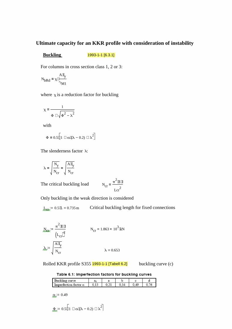
Ultimate capacity for an KKR profile with consideration of instability
Buckling 1993-1-1 [6.3.1]
For columns in cross section class 1, 2 or 3:
NbRd χA fy⋅
γM1⋅=
where χ is a reduction factor for buckling
χ1
Φ Φ2
λ2−+
=
with
Φ 0.5 1 α λ 0.2−( )⋅+ λ2+ ⋅=
The slenderness factor λ:
λNy
Ncr=
A fy⋅
Ncr=
The critical buckling load Ncrπ
2E⋅ I⋅
Lcr2
=
Only buckling in the weak direction is considered
Lcr 0.5 L⋅ 0.735m=:= Critical buckling length for fixed connections
Ncrπ
2E⋅ I⋅
Lcr( )2:= Ncr 1.863 10
3× kN⋅=
λA fy⋅
Ncr:=
λ 0.653=
Rolled KKR profile S355 1993-1-1 [Tabell 6.2] buckling curve (c)
α 0.49:=
Φ 0.5 1 α λ 0.2−( )⋅+ λ2+ ⋅:=
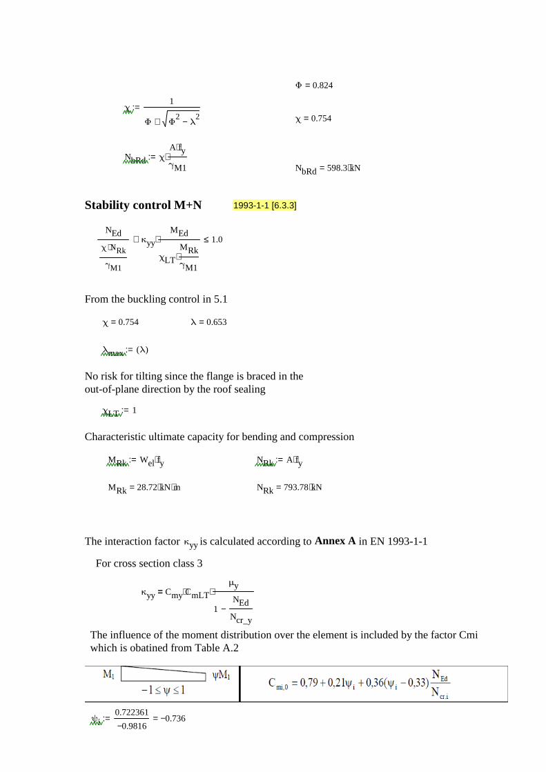
Φ 0.824=
χ1
Φ Φ2
λ2−+
:=χ 0.754=
NbRd χA fy⋅
γM1⋅:=
NbRd 598.3 kN⋅=
Stability control M+N 1993-1-1 [6.3.3]
NEd
χ NRk⋅
γM1
κyy
MEd
χLT
MRk
γM1⋅
⋅+ 1.0≤
From the buckling control in 5.1
χ 0.754= λ 0.653=
λmax λ( ):=
No risk for tilting since the flange is braced in theout-of-plane direction by the roof sealing
χLT 1:=
Characteristic ultimate capacity for bending and compression
MRk Wel fy⋅:= NRk A fy⋅:=
MRk 28.72 kN m⋅⋅= NRk 793.78 kN⋅=
The interaction factor κyy is calculated according to Annex A in EN 1993-1-1
For cross section class 3
κyy Cmy CmLT⋅μy
1NEd
Ncr_y−
⋅=
The influence of the moment distribution over the element is included by the factor Cmiwhich is obatined from Table A.2
ψi0.722361
0.9816−0.736−=:=
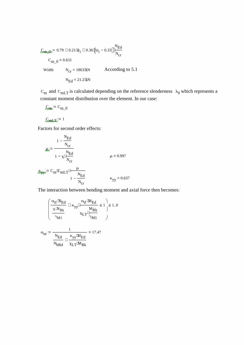
Cm_0 0.79 0.21ψi⋅+ 0.36 ψi 0.33−( )⋅NEd
Ncr⋅+:=
Cm_0 0.631=
Width Ncr 1863 kN⋅= According to 5.1
NEd 21.2 kN⋅=
Cm and CmLT is calculated depending on the reference slenderness λ0 which represents a
constant moment distribution over the element. In our case:
Cm Cm_0:=
CmLT 1:=
Factors for second order effects:
μ
1NEd
Ncr−
1 χNEd
Ncr⋅−
:=
μ 0.997=
κyy Cm CmLT⋅μ
1NEd
Ncr−
⋅:=
κyy 0.637=
The interaction between bending moment and axial force then becomes:
αtf NEd⋅
χ NRk⋅
γM1
κyy
αtf MEd⋅
χLT
MRk
γM1⋅
⋅+ 1≤
1≤ 0,
αut1
NEd
NbRd
κyy MEd⋅
χLT MRk⋅+
17.47=:=
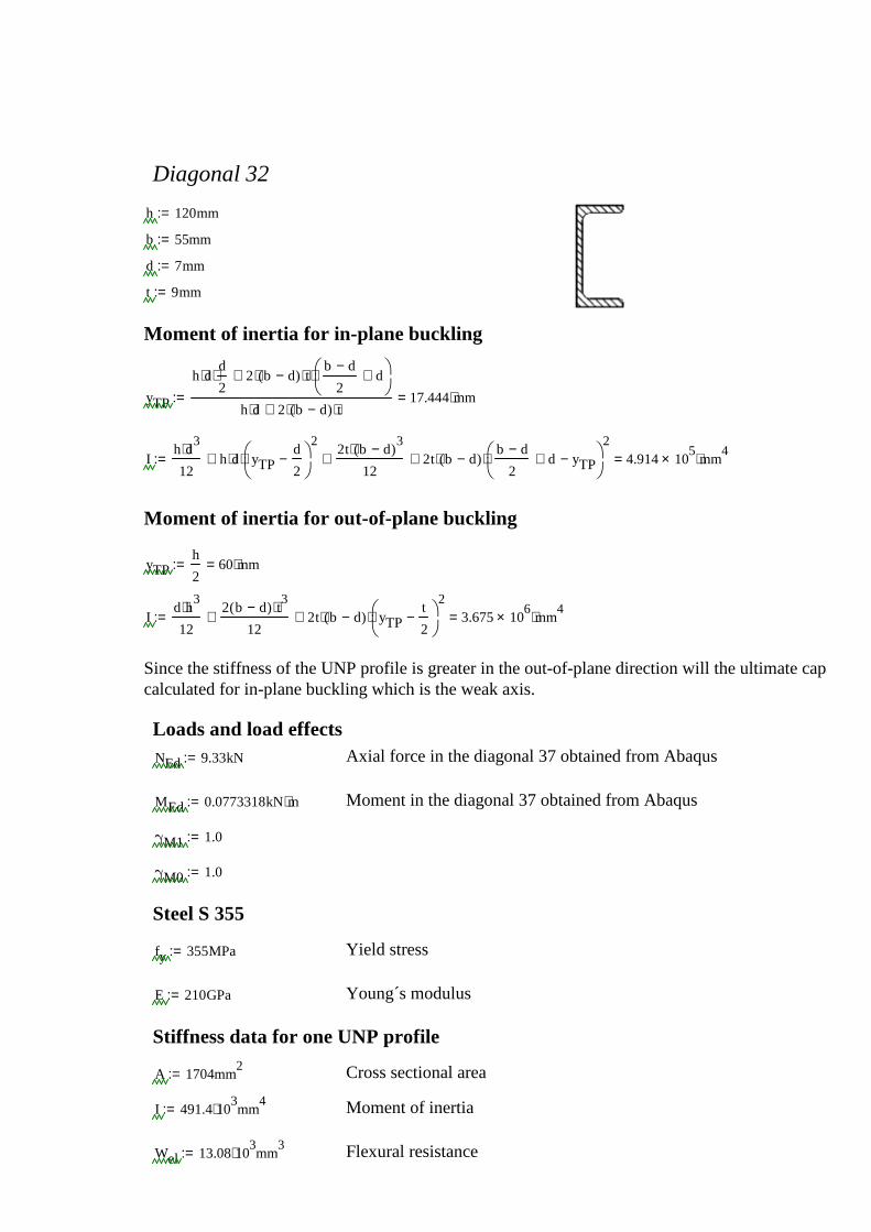
Diagonal 32
h 120mm:=
b 55mm:=
d 7mm:=
t 9mm:=
Moment of inertia for in-plane buckling
yTP
h d⋅d
2⋅ 2 b d−( )⋅ t⋅
b d−2
d+
⋅+
h d⋅ 2 b d−( )⋅ t⋅+17.444 mm⋅=:=
Ih d
3⋅12
h d⋅ yTPd
2−
2
⋅+2t b d−( )
3⋅12
+ 2t b d−( )⋅b d−
2d+ yTP−
2
⋅+ 4.914 105× mm
4⋅=:=
Moment of inertia for out-of-plane buckling
yTPh
260 mm⋅=:=
Id h
3⋅12
2 b d−( ) t3⋅
12+ 2t b d−( )⋅ yTP
t
2−
2
⋅+ 3.675 106× mm
4⋅=:=
Since the stiffness of the UNP profile is greater in the out-of-plane direction will the ultimate capacity becalculated for in-plane buckling which is the weak axis.
Loads and load effectsNEd 9.33kN:= Axial force in the diagonal 37 obtained from Abaqus
MEd 0.0773318kN m⋅:= Moment in the diagonal 37 obtained from Abaqus
γM1 1.0:=
γM0 1.0:=
Steel S 355
fy 355MPa:= Yield stress
E 210GPa:= Young´s modulus
Stiffness data for one UNP profile
A 1704mm2:= Cross sectional area
I 491.4 103⋅ mm
4:= Moment of inertia
Wel 13.08 103⋅ mm
3:= Flexural resistance
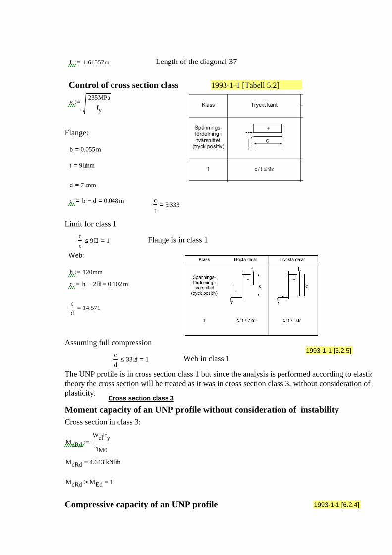
L 1.61557m:= Length of the diagonal 37
Control of cross section class 1993-1-1 [Tabell 5.2]
ε235MPa
fy:=
Flange:
b 0.055m=
t 9 mm⋅=
d 7 mm⋅=
c b d− 0.048m=:= c
t5.333=
Limit for class 1
c
t9 ε⋅≤ 1= Flange is in class 1
Web:
h 120mm:=
c h 2 t⋅− 0.102m=:=
c
d14.571=
Assuming full compression1993-1-1 [6.2.5]
c
d33 ε⋅≤ 1= Web in class 1
The UNP profile is in cross section class 1 but since the analysis is performed according to elastictheory the cross section will be treated as it was in cross section class 3, without consideration ofplasticity.
Cross section class 3
Moment capacity of an UNP profile without consideration of instabilityCross section in class 3:
McRd
Wel fy⋅
γM0:=
McRd 4.643 kN m⋅⋅=
McRd MEd> 1=
Compressive capacity of an UNP profile 1993-1-1 [6.2.4]
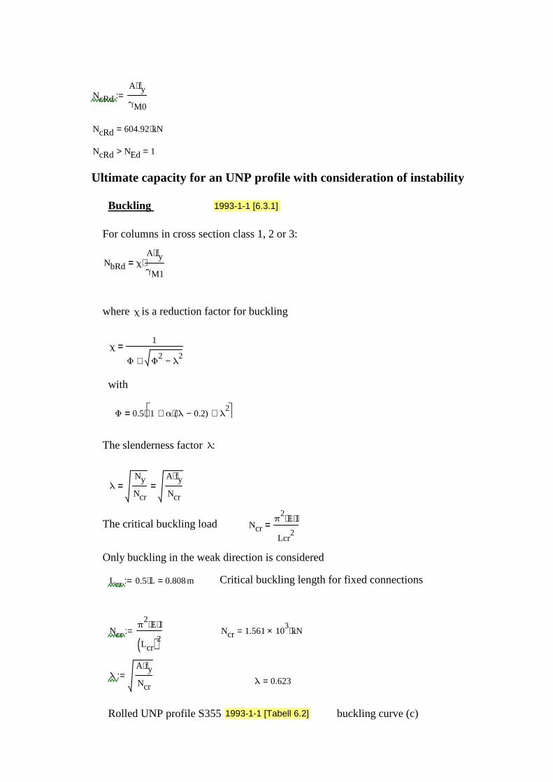
NcRd
A fy⋅
γM0:=
NcRd 604.92 kN⋅=
NcRd NEd> 1=
Ultimate capacity for an UNP profile with consideration of instability
Buckling 1993-1-1 [6.3.1]
For columns in cross section class 1, 2 or 3:
NbRd χA fy⋅
γM1⋅=
where χ is a reduction factor for buckling
χ1
Φ Φ2
λ2−+
=
with
Φ 0.5 1 α λ 0.2−( )⋅+ λ2+ ⋅=
The slenderness factor λ:
λNy
Ncr=
A fy⋅
Ncr=
The critical buckling load Ncrπ
2E⋅ I⋅
Lcr2
=
Only buckling in the weak direction is considered
Lcr 0.5 L⋅ 0.808m=:= Critical buckling length for fixed connections
Ncrπ
2E⋅ I⋅
Lcr( )2:= Ncr 1.561 10
3× kN⋅=
λA fy⋅
Ncr:=
λ 0.623=
Rolled UNP profile S355 1993-1-1 [Tabell 6.2] buckling curve (c)
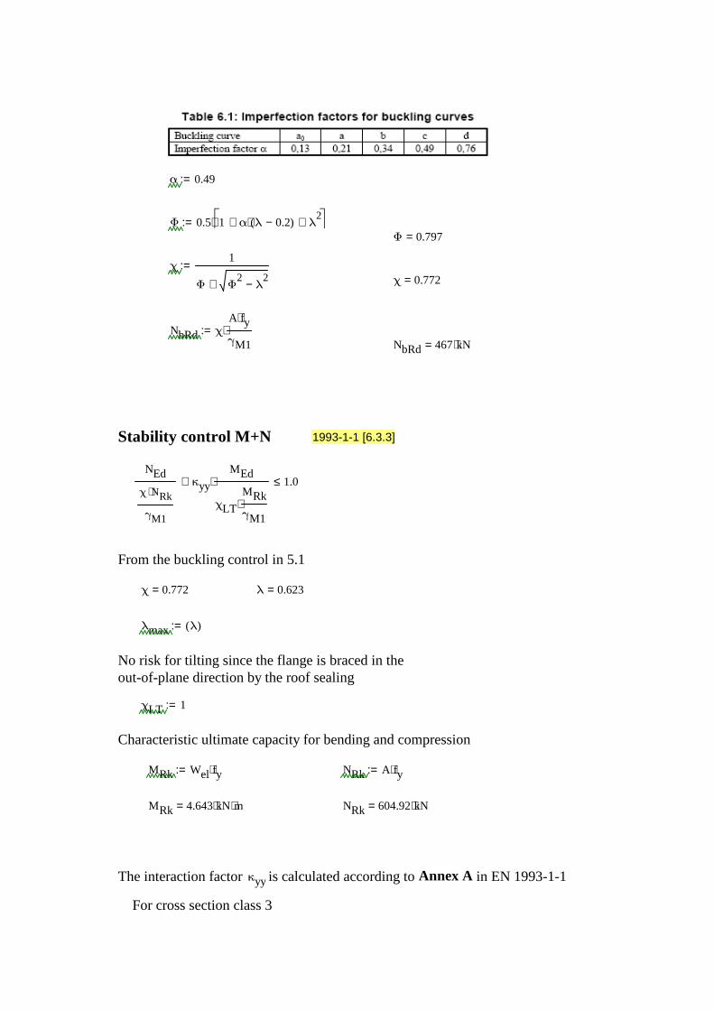
α 0.49:=
Φ 0.5 1 α λ 0.2−( )⋅+ λ2+ ⋅:=
Φ 0.797=
χ1
Φ Φ2
λ2−+
:=χ 0.772=
NbRd χA fy⋅
γM1⋅:=
NbRd 467 kN⋅=
Stability control M+N 1993-1-1 [6.3.3]
NEd
χ NRk⋅
γM1
κyy
MEd
χLT
MRk
γM1⋅
⋅+ 1.0≤
From the buckling control in 5.1
χ 0.772= λ 0.623=
λmax λ( ):=
No risk for tilting since the flange is braced in theout-of-plane direction by the roof sealing
χLT 1:=
Characteristic ultimate capacity for bending and compression
MRk Wel fy⋅:= NRk A fy⋅:=
MRk 4.643 kN m⋅⋅= NRk 604.92 kN⋅=
The interaction factor κyy is calculated according to Annex A in EN 1993-1-1
For cross section class 3
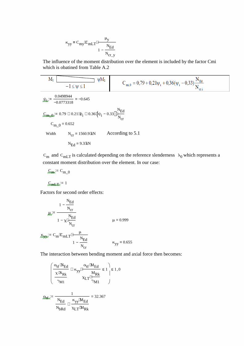
κyy Cmy CmLT⋅μy
1NEd
Ncr_y−
⋅=
The influence of the moment distribution over the element is included by the factor Cmiwhich is obatined from Table A.2
ψi0.0498944
0.0773318−0.645−=:=
Cm_0 0.79 0.21ψi⋅+ 0.36 ψi 0.33−( )⋅NEd
Ncr⋅+:=
Cm_0 0.652=
Width Ncr 1560.9 kN⋅= According to 5.1
NEd 9.3 kN⋅=
Cm and CmLT is calculated depending on the reference slenderness λ0 which represents a
constant moment distribution over the element. In our case:
Cm Cm_0:=
CmLT 1:=
Factors for second order effects:
μ
1NEd
Ncr−
1 χNEd
Ncr⋅−
:=
μ 0.999=
κyy Cm CmLT⋅μ
1NEd
Ncr−
⋅:=
κyy 0.655=
The interaction between bending moment and axial force then becomes:
αtf NEd⋅
χ NRk⋅
γM1
κyy
αtf MEd⋅
χLT
MRk
γM1⋅
⋅+ 1≤
1≤ 0,
αtf1
NEd
NbRd
κyy MEd⋅
χLT MRk⋅+
32.367=:=
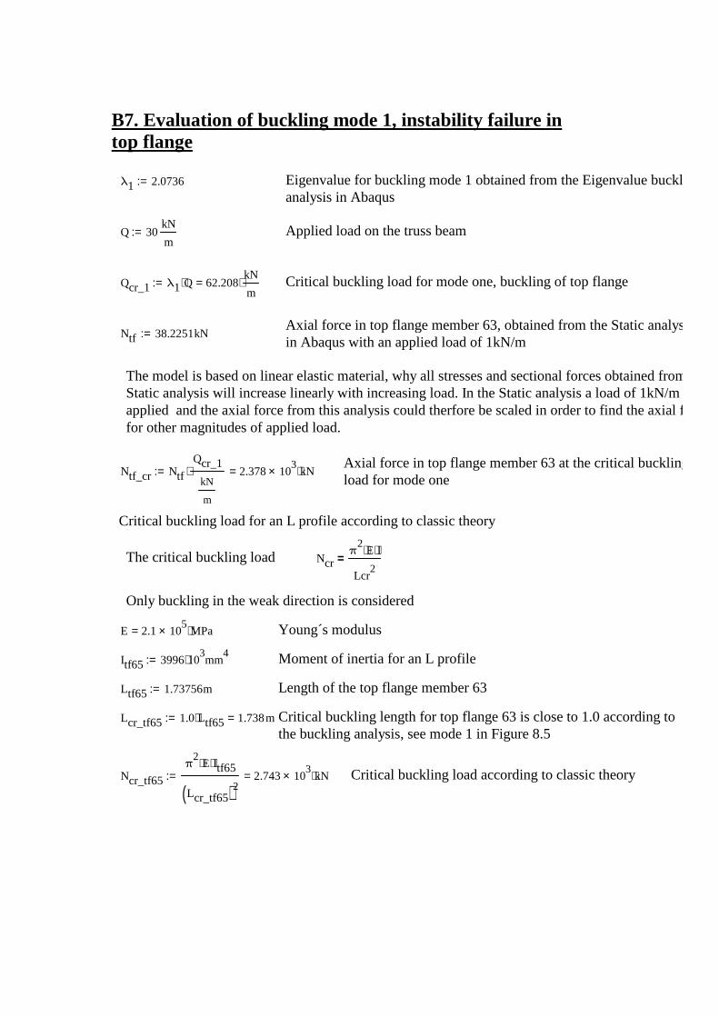
B7. Evaluation of buckling mode 1, instability failure intop flange
λ1 2.0736:= Eigenvalue for buckling mode 1 obtained from the Eigenvalue buckling analysis in Abaqus
Q 30kN
m:= Applied load on the truss beam
Qcr_1 λ1 Q⋅ 62.208kN
m⋅=:= Critical buckling load for mode one, buckling of top flange
Axial force in top flange member 63, obtained from the Static analysisin Abaqus with an applied load of 1kN/m
Ntf 38.2251kN:=
The model is based on linear elastic material, why all stresses and sectional forces obtained from theStatic analysis will increase linearly with increasing load. In the Static analysis a load of 1kN/m isapplied and the axial force from this analysis could therfore be scaled in order to find the axial forcefor other magnitudes of applied load.
Axial force in top flange member 63 at the critical bucklingload for mode one
Ntf_cr Ntf
Qcr_1
kN
m
⋅ 2.378 103× kN⋅=:=
Critical buckling load for an L profile according to classic theory
The critical buckling load Ncrπ
2E⋅ I⋅
Lcr2
=
Only buckling in the weak direction is considered
E 2.1 105× MPa⋅= Young´s modulus
Itf65 3996 103⋅ mm
4:= Moment of inertia for an L profile
Ltf65 1.73756m:= Length of the top flange member 63
Lcr_tf65 1.0 Ltf65⋅ 1.738m=:= Critical buckling length for top flange 63 is close to 1.0 according tothe buckling analysis, see mode 1 in Figure 8.5
Ncr_tf65
π2
E⋅ Itf65⋅
Lcr_tf65( )22.743 10
3× kN⋅=:= Critical buckling load according to classic theory
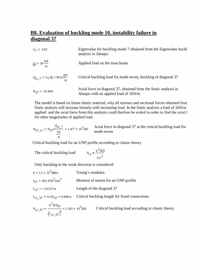
B8. Evaluation of buckling mode 10, instability failure indiagonal 37
λ7 3.02:= Eigenvalue for buckling mode 7 obtained from the Eigenvalue buckling analysis in Abaqus
Q 30kN
m:= Applied load on the truss beam
Qcr_7 λ7 Q⋅ 90.6kN
m⋅=:= Critical buckling load for mode seven, buckling of diagonal 37
Axial force in diagonal 37, obtained from the Static analysis inAbaqus with an applied load of 1kN/m
N37 16.3kN:=
The model is based on linear elastic material, why all stresses and sectional forces obtained from theStatic analysis will increase linearly with increasing load. In the Static analysis a load of 1kN/m isapplied and the axial force from this analysis could therfore be scaled in order to find the axial forcefor other magnitudes of applied load.
Axial force in diagonal 37 at the critical buckling load formode seven
N37_cr N37
Qcr_7
kN
m
⋅ 1.477 103× kN⋅=:=
Critical buckling load for an UNP profile according to classic theory
The critical buckling load Ncrπ
2E⋅ I⋅
Lcr2
=
Only buckling in the weak direction is considered
E 2.1 105× MPa⋅= Young´s modulus
I37 491.4 103⋅ mm
4:= Moment of inertia for an UNP profile
L37 1.61557m:= Length of the diagonal 37
Lcr_37 0.5 L37⋅ 0.808m=:= Critical buckling length for fixed connections
Ncr_37
π2
E⋅ I37⋅
Lcr_37( )21.561 10
3× kN⋅=:= Critical buckling load according to classic theory
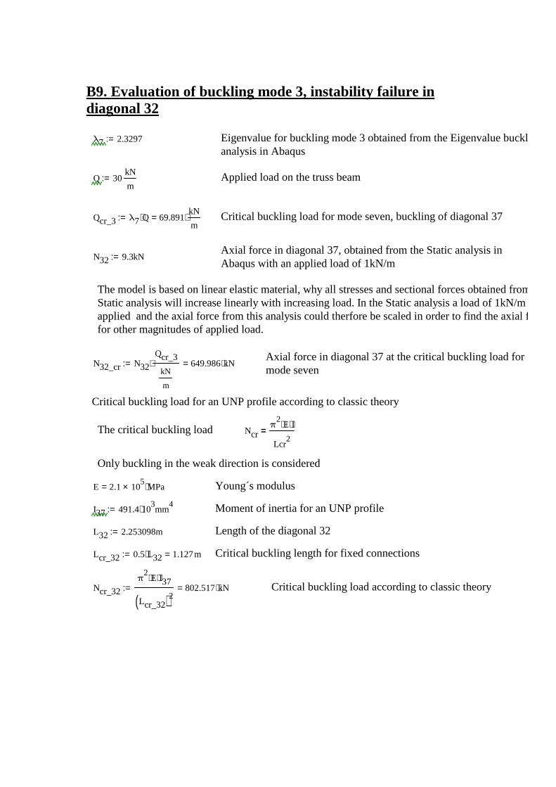
B9. Evaluation of buckling mode 3, instability failure indiagonal 32
λ7 2.3297:= Eigenvalue for buckling mode 3 obtained from the Eigenvalue buckling analysis in Abaqus
Q 30kN
m:= Applied load on the truss beam
Qcr_3 λ7 Q⋅ 69.891kN
m⋅=:= Critical buckling load for mode seven, buckling of diagonal 37
Axial force in diagonal 37, obtained from the Static analysis inAbaqus with an applied load of 1kN/m
N32 9.3kN:=
The model is based on linear elastic material, why all stresses and sectional forces obtained from theStatic analysis will increase linearly with increasing load. In the Static analysis a load of 1kN/m isapplied and the axial force from this analysis could therfore be scaled in order to find the axial forcefor other magnitudes of applied load.
Axial force in diagonal 37 at the critical buckling load formode seven
N32_cr N32
Qcr_3
kN
m
⋅ 649.986 kN⋅=:=
Critical buckling load for an UNP profile according to classic theory
The critical buckling load Ncrπ
2E⋅ I⋅
Lcr2
=
Only buckling in the weak direction is considered
E 2.1 105× MPa⋅= Young´s modulus
I37 491.4 103⋅ mm
4:= Moment of inertia for an UNP profile
L32 2.253098m:= Length of the diagonal 32
Lcr_32 0.5 L32⋅ 1.127m=:= Critical buckling length for fixed connections
Ncr_32
π2
E⋅ I37⋅
Lcr_32( )2802.517 kN⋅=:= Critical buckling load according to classic theory
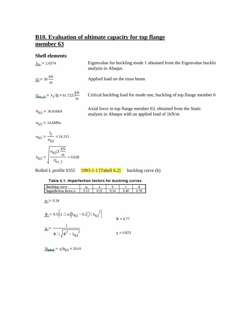
B10. Evaluation of ultimate capacity for top flangemember 63
Shell elementsλ1 2.0574:= Eigenvalue for buckling mode 1 obtained from the Eigenvalue buckling
analysis in Abaqus
Q 30kN
m:= Applied load on the truss beam
Qcr_1 λ1 Q⋅ 61.722kN
m⋅=:= Critical buckling load for mode one, buckling of top flange member 63
Axial force in top flange member 63, obtained from the Staticanalysis in Abaqus with an applied load of 1kN/m
N63 36.816kN:=
σ63 14.6MPa:=
α63
fy
σ6324.315=:=
λ63
α63 1⋅kN
m
Qcr_10.628=:=
Rolled L profile S355 1993-1-1 [Tabell 6.2] buckling curve (b)
α 0.34:=
Φ 0.5 1 α λ63 0.2−( )⋅+ λ632+
⋅:=
Φ 0.77=
χ1
Φ Φ2
λ632−+
:=χ 0.823=
NbRd χ α63⋅ 20.01=:=
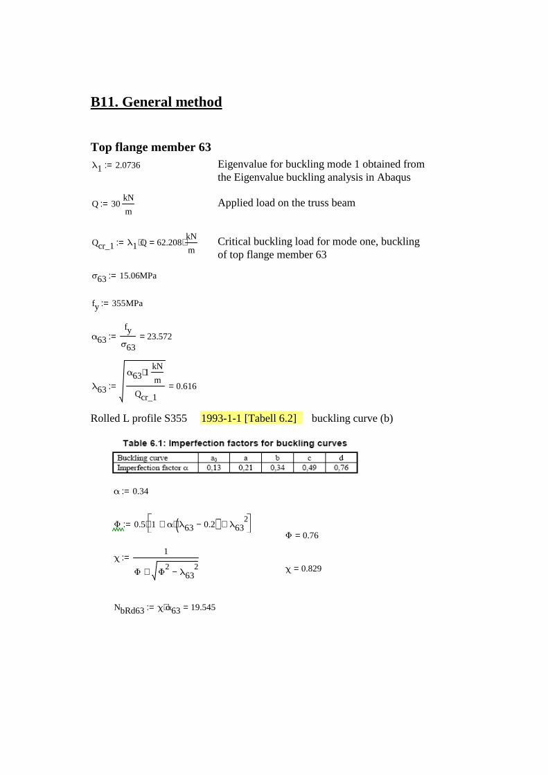
B11. General method
Top flange member 63λ1 2.0736:= Eigenvalue for buckling mode 1 obtained from
the Eigenvalue buckling analysis in Abaqus
Q 30kN
m:= Applied load on the truss beam
Qcr_1 λ1 Q⋅ 62.208kN
m⋅=:= Critical buckling load for mode one, buckling
of top flange member 63
σ63 15.06MPa:=
fy 355MPa:=
α63
fy
σ6323.572=:=
λ63
α63 1⋅kN
m
Qcr_10.616=:=
Rolled L profile S355 1993-1-1 [Tabell 6.2] buckling curve (b)
α 0.34:=
Φ 0.5 1 α λ63 0.2−( )⋅+ λ632+
⋅:=
Φ 0.76=
χ1
Φ Φ2
λ632−+
:=χ 0.829=
NbRd63 χ α63⋅ 19.545=:=

Diagonal 32λ2 2.3297:= Eigenvalue for buckling mode 1 obtained from the
Eigenvalue buckling analysis in Abaqus
Q 30kN
m:= Applied load on the truss beam
Qcr_2 λ2 Q⋅ 69.891kN
m⋅=:= Critical buckling load for mode one, buckling of
diagonal 32
σ32 11.4MPa:=
fy 355MPa:=
α32
fy
σ3231.14=:=
λ32
α32 1⋅kN
m
Qcr_20.667=:=
UNP profile 1993-1-1 [Tabell 6.2] buckling curve (c)
α 0.49:=
Φ 0.5 1 α λ32 0.2−( )⋅+ λ322+
⋅:=
Φ 0.837=
χ1
Φ Φ2
λ322−+
:=χ 0.745=
NbRd32 χ α32⋅ 23.19=:=
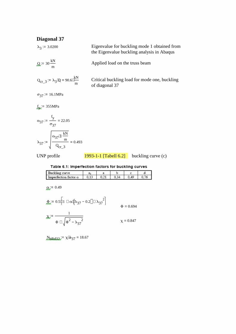
Diagonal 37λ3 3.0200:= Eigenvalue for buckling mode 1 obtained from
the Eigenvalue buckling analysis in Abaqus
Q 30kN
m:= Applied load on the truss beam
Qcr_3 λ3 Q⋅ 90.6kN
m⋅=:= Critical buckling load for mode one, buckling
of diagonal 37
σ37 16.1MPa:=
fy 355MPa:=
α37
fy
σ3722.05=:=
λ37
α37 1⋅kN
m
Qcr_30.493=:=
UNP profile 1993-1-1 [Tabell 6.2] buckling curve (c)
α 0.49:=
Φ 0.5 1 α λ37 0.2−( )⋅+ λ372+
⋅:=
Φ 0.694=
χ1
Φ Φ2
λ372−+
:=χ 0.847=
NbRd32 χ α37⋅ 18.67=:=