modelling of repairable items for production inventory with random deterioration
TRANSCRIPT
IOSR Journal of Mathematics (IOSR-JM)
e-ISSN: 2278-5728, p-ISSN: 2319-765X. Volume 11, Issue 1 Ver. IV (Jan - Feb. 2015), PP 56-69 www.iosrjournals.org
DOI: 10.9790/5728-11145669 www.iosrjournals.org 56 |Page
Modelling of repairable items for production inventory with
random deterioration
Dr.Ravish Kumar Yadav1, RajeevKumar
2
1,Associate Professor ,Department of mathematics ,Hindu College, Moradbad, 2Devta Mahavidhyal, Bijnoor
Abstract: Keeping in view the concern about environmental protection, the study incorporate the concept of
repairing in a production inventory model consisting of production system and repairing system over infinite
planning horizon. This study presents a forward production and reverse repairing system inventory model with
a time dependent random deterioration function and increasing exponentially demand with the finite production
rate is proportional to the demand rate at any instant. The shortages allow and excess demand is backlogged.
Expressions for optimal parameter are obtained .We also obtained Production and repairing scheduling period,
maximum inventory level and total average cost. Using calculus, optimum production policy is derived, which
minimizes the total cost incurred
I. Introduction An inventory system the effect of deterioration plays an important role. Deterioration is derived as
decay or damage such that the item cannot be used for its original propose. Foods, pharmaceuticals, chemicals, blood, drugs are a few examples of such items in which sufficient deterioration can take place during the storage
period of the units and the importance of this loss must be taken into account when analyzing the system.
When describing optimum policies for deteriorating items Ghare and Schrader (1963) proposed a
constant rate of deterioration and constant rate demand. In recent year, inventory problem for deterioration items
have been widely studied after Ghare and Schrader (1963), Covert and Philip (1973) formulated the model
for variable deterioration rate with two parameters Weibull disturbation Goswami and Chaudhuri (1991),
Bose et al (1995) assumed either instantaneous or finite production with different assumption on the pattern of
deterioration.
Balkhi and Benkheroot (1996) considered a production a production lot size inventory model with
arbitrary production and demand rate depends on the time function.
Bhunia and Maiti’s (1977) model to formulate a production inventory model. Chang and Deve
(1999) investigated an EOQ model allow shortage and backlogging. It is assumed that the backlogging rate is
variable and dependent on the length of waiting time for the next replenishment. Recently, many researchers
have modified inventory policies by considering the “ time proportional partial backlogging rate” such as Wang
(2002), Perumal (2002), Teng et al (2003), Skouri and Papachristos (2003) etc.
Schrady (1967) first studied the problem on optimal lot sizes for production/procurement and
recovery. For issues in the greening process, Nahmias and Rivera (1979) studied an EPQ variant of Schrady‟s
model (1967) with a finite recovery rate. Richter (1996a, 1996b, 1997) and Richter and Dobos (1999)
investigated a waste disposal model by considering the returned rate as a decision variable. Dobos and Richter
(2003, 2004) investigated a production/remanufacturing system with constant demand that is satisfied by
noninstantaneous production and remanufacturing for single and multiple remanufacturing and production
cycle. Dobos and Richter (2006) extended their previous model and assumed that the quality of collected
returned items is not always suitable for further repairing. Konstantaras and Skouri (2010) presented a model by considering a general cycle pattern in which a variable number of reproduction lots of equal size were
followed by a variable number of manufacturing lots of equal size. They also studied a special case where
shortages were allowed in each manufacturing and reproduction cycle and similar sufficient conditions, as the
non-shortages case, are given.El Saadany and Jaber (2010) extended the models developed by Dobos and
Richter (2003, 2004) by assuming that the collection rate of returned items is dependent on the purchasing price
and the acceptance quality level of these returns. That is, the flow of used/returned items increases as the
purchasing price increases, and decreases as the corresponding acceptance quality level increases. Alamri
(2010) developed a general reverse logistics inventory model. Chung and Wee (2011) developed an inventory
model on short life-cycle deteriorating product remanufacturing in a green supply chain model
In this paper we present a realistic inventory model in which the production rate depends on the
demand and demand is an exponentially increasing function time and deterioration is random function says that deterioration of an item depends upon the fluctuation of humidity, temperature, etc. It would be more reasonable
and realistic if we assume the deterioration function to depend upon a parameter "" in addition to time t
Modelling of repairable items for production inventory with random deterioration
DOI: 10.9790/5728-11145669 www.iosrjournals.org 57 |Page
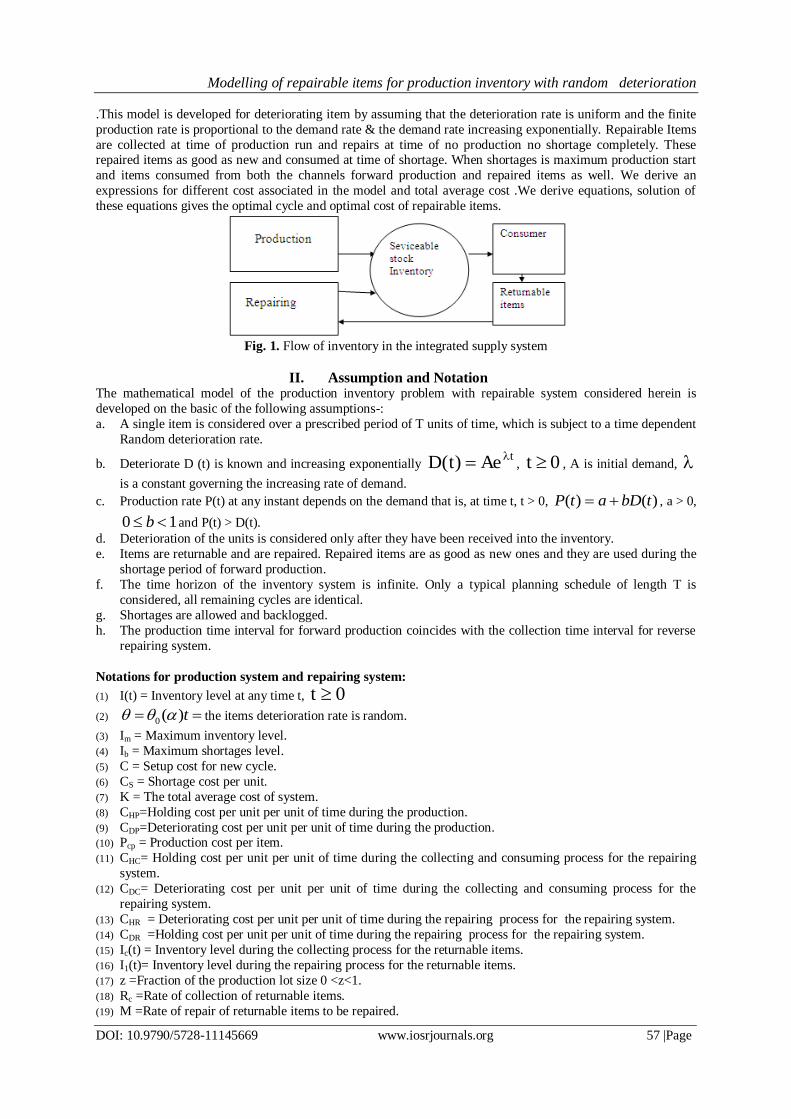
.This model is developed for deteriorating item by assuming that the deterioration rate is uniform and the finite
production rate is proportional to the demand rate & the demand rate increasing exponentially. Repairable Items
are collected at time of production run and repairs at time of no production no shortage completely. These repaired items as good as new and consumed at time of shortage. When shortages is maximum production start
and items consumed from both the channels forward production and repaired items as well. We derive an
expressions for different cost associated in the model and total average cost .We derive equations, solution of
these equations gives the optimal cycle and optimal cost of repairable items.
Fig. 1. Flow of inventory in the integrated supply system
II. Assumption and Notation The mathematical model of the production inventory problem with repairable system considered herein is
developed on the basic of the following assumptions-:
a. A single item is considered over a prescribed period of T units of time, which is subject to a time dependent
Random deterioration rate.
b. Deteriorate D (t) is known and increasing exponentially tAe)t(D , 0t , A is initial demand,
is a constant governing the increasing rate of demand.
c. Production rate P(t) at any instant depends on the demand that is, at time t, t > 0, )()( tbDatP , a > 0,
10 b and P(t) > D(t).
d. Deterioration of the units is considered only after they have been received into the inventory.
e. Items are returnable and are repaired. Repaired items are as good as new ones and they are used during the
shortage period of forward production.
f. The time horizon of the inventory system is infinite. Only a typical planning schedule of length T is
considered, all remaining cycles are identical.
g. Shortages are allowed and backlogged.
h. The production time interval for forward production coincides with the collection time interval for reverse
repairing system.
Notations for production system and repairing system:
(1) I(t) = Inventory level at any time t, 0t
(2) 0( )t the items deterioration rate is random.
(3) Im = Maximum inventory level.
(4) Ib = Maximum shortages level.
(5) C = Setup cost for new cycle.
(6) CS = Shortage cost per unit.
(7) K = The total average cost of system.
(8) CHP=Holding cost per unit per unit of time during the production.
(9) CDP=Deteriorating cost per unit per unit of time during the production. (10) Pcp = Production cost per item.
(11) CHC= Holding cost per unit per unit of time during the collecting and consuming process for the repairing
system.
(12) CDC= Deteriorating cost per unit per unit of time during the collecting and consuming process for the
repairing system.
(13) CHR = Deteriorating cost per unit per unit of time during the repairing process for the repairing system.
(14) CDR =Holding cost per unit per unit of time during the repairing process for the repairing system.
(15) Ic(t) = Inventory level during the collecting process for the returnable items.
(16) I1(t)= Inventory level during the repairing process for the returnable items.
(17) z =Fraction of the production lot size 0 <z<1.
(18) Rc =Rate of collection of returnable items.
(19) M =Rate of repair of returnable items to be repaired.
Modelling of repairable items for production inventory with random deterioration
DOI: 10.9790/5728-11145669 www.iosrjournals.org 58 |Page
(20) t1 = Time when production stops and also the time when collecting process for returnable items stops. At
this very time repairing of collected items start.
(21) t2 = Time period when repairing of returnable items stops and also the time when accumulated inventory of production system vanishes.
(22) t3 = Time when shortages is maximum.(t= t1+ t2+ t3)
(23) t4 = Period of time when production starts again during the period of shortage.
(24) T = )( 4321 tttt is the cycle time.
(25) IS = Maximum inventory level of repaired items.
(26) Pcc= Cost of purchasing the returnable items per unit.
(27) Pcr =Repair cost of repaired items per unit.
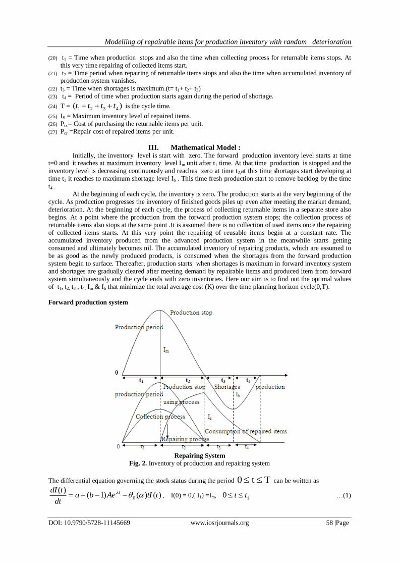
III. Mathematical Model : Initially, the inventory level is start with zero. The forward production inventory level starts at time
t=0 and it reaches at maximum inventory level Im unit after t1 time. At that time production is stopped and the
inventory level is decreasing continuously and reaches zero at time t2,at this time shortages start developing at
time t3 it reaches to maximum shortage level Ib . This time fresh production start to remove backlog by the time
t4 .
At the beginning of each cycle, the inventory is zero. The production starts at the very beginning of the
cycle. As production progresses the inventory of finished goods piles up even after meeting the market demand,
deterioration. At the beginning of each cycle, the process of collecting returnable items in a separate store also
begins. At a point where the production from the forward production system stops; the collection process of
returnable items also stops at the same point .It is assumed there is no collection of used items once the repairing
of collected items starts. At this very point the repairing of reusable items begin at a constant rate. The
accumulated inventory produced from the advanced production system in the meanwhile starts getting consumed and ultimately becomes nil. The accumulated inventory of repairing products, which are assumed to
be as good as the newly produced products, is consumed when the shortages from the forward production
system begin to surface. Thereafter, production starts when shortages is maximum in forward inventory system
and shortages are gradually cleared after meeting demand by repairable items and produced item from forward
system simultaneously and the cycle ends with zero inventories. Here our aim is to find out the optimal values
of t1, t2, t3 , t4, Im & Ib that minimize the total average cost (K) over the time planning horizon cycle(0,T).
Forward production system
Repairing System
Fig. 2. Inventory of production and repairing system
The differential equation governing the stock status during the period Tt0 can be written as
)()()1()(
0 ttIAebadt
tdI t , I(0) = 0,( I1) =Im, 10 tt …(1)
Modelling of repairable items for production inventory with random deterioration
DOI: 10.9790/5728-11145669 www.iosrjournals.org 59 |Page
0
( )( ) ( )tdI t
Ae tI tdt
, I(t1) =Im , I(t2) = 0 , 20 tt
… (2)
( ) tdI tAe
dt
, I(0) =o, I(t3) =Ib,
,30 t t ….(3)
( )( 1) tdI t
a b Aedt
, I(0) = Ib,I(t4)=0,40 t t
….(4)
Differential equations representing repairing system in collecting time & consuming time
0
( )( ) t ( )c
c c
dI tR I t
dt , Ic(0) = 0
10 tt … (5)
0
( )( ) t ( )c
c
dI tM I t
dt , Ic(t1) = Bz , 20 t t … (6)
Where
B=Production lot size during production system=Production- Deterioration
1 1 1
1
1
0 0
0 0 0
0
0
2
0 0 1 00 1
( ) (1 ( ) )(a bAe )
{a bAe ( ) (a bAe )}
( ) ( ) ( )bA bAe{ (1 ) } {1 ( ) ) }
2
t t t
t
t
t t
t
Pdt tPdt t dt
t dt
a tt
Differential equations representing inventory of repaired items.
1
0 1
( )( ) t ( )
dI tM I t
dt
,
I1(0) = 0, I1(t2) =Is, 20 t t , ….(7)
0
( )( ) ( )tdI t
Ae tI tdt
,I(0) =Is,I 3 4( ) 0t t , I(t3) =Ib1 , 3 40 t t t
… (8)
Solution of equation (1) , (2) , .3) and (4) by adjusting the constant of integration using boundary condition are
given by
t
Aeb
et
tatIt
t
t )(1
)1(
6
)()( 02
)(
2)(3
0
02
0
t
t
eet
2
0
2
0
2
0 )()(
2
)(
,
10 tt
… (9)
)(tI
A
2
020
2
02)( )()(
2
)(1
22
0
tte
et
t
2
00
2
0 )()(
2
)(1
tte t
,
20 t t … (10)
)(tI )1( teA
, 30 t t … (11)
)()1(
)()( 4
4
tt eebA
ttatI
,40 t t … (12)
Solving (5) and (6)
Modelling of repairable items for production inventory with random deterioration
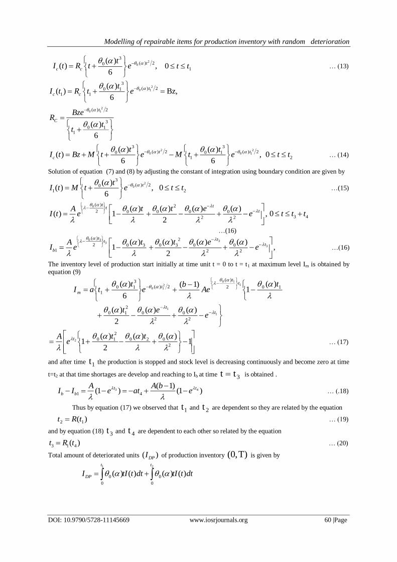
DOI: 10.9790/5728-11145669 www.iosrjournals.org 60 |Page
20
3( ) 20 ( )
( ) ,6
t
c c
tI t R t e
10 tt
… (13)
20 1
20 1
3( ) 20 1
1 1
( ) 2
3
0 11
( )( ) Bz,
6
( )
6
t
c c
t
C
tI t R t e
BzeR
tt
2 20 0 1
3 3( ) 2 ( ) 20 0 1
1
( ) ( )( ) ,
6 6
t t
c
t tI t Bz M t e M t e
20 t t
… (14)
Solution of equation (7) and (8) by adjusting the constant of integration using boundary condition are given by
20
3( ) 20
1
( )( ) ,
6
ttI t M t e
20 t t
…(15)
0 ( )
2 0 ( )( ) 1
tt tA
I t e
2
0 0 0
2 2
( ) ( ) ( ),
2
ttt e
e
3 40 t t t
…(16)
0 33
( )
2 0 31
( )1
tt
b
tAI e
3
3
2
0 3 0 0
2 2
( ) ( ) ( ),
2
ttt e
e
…(16)
The inventory level of production start initially at time unit t = 0 to t = t1 at maximum level Im is obtained by
equation (9)
102
)(
2)(3
10
1
)(1
)1(
6
)( 110
210
tAe
be
ttaI
tt
t
m
1
1
2
0
2
0
2
10 )()(
2
)( tt
eet
1)()(
2
)(1
2
020
2
102
tte
A t … (17)
and after time 1t the production is stopped and stock level is decreasing continuously and become zero at time
t=t2 at that time shortages are develop and reaching to Ib at time 3tt is obtained .
3 4
1 4
( 1)(1 ) (1 )
t t
b b
A A bI I e at e
… (.18)
Thus by equation (17) we observed that 1t and 2t are dependent so they are related by the equation
)( 12 tRt … (19)
and by equation (18) 3t and 4t are dependent to each other so related by the equation
3 1 4( )t R t … (20)
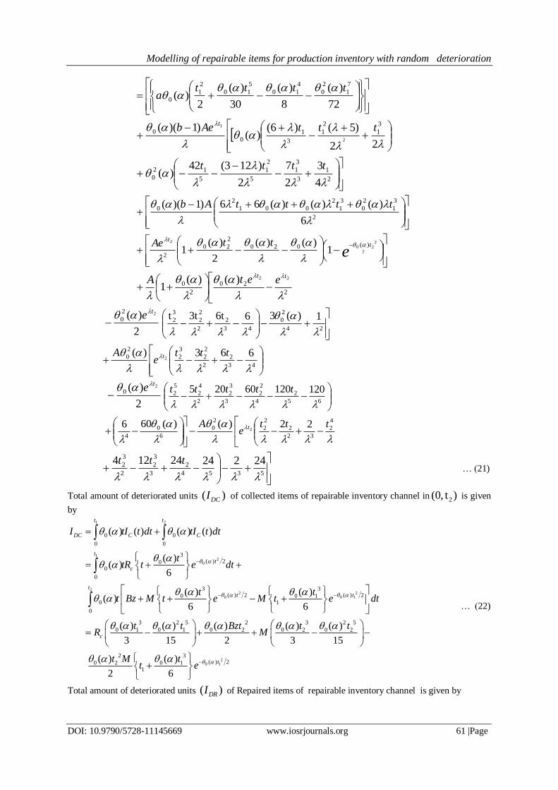
Total amount of deteriorated units ( )DPI of production inventory )T,0( is given by
1 2
0 0
0 0
( ) ( ) ( ) ( )
t t
DPI tI t dt tI t dt
Modelling of repairable items for production inventory with random deterioration
DOI: 10.9790/5728-11145669 www.iosrjournals.org 61 |Page
72
)(
8
)(
30
)(
2)(
7
1
2
0
4
10
5
10
2
1
0
tttta
22
)5()6()(
)1)(( 3
1
2
1
3
1
0
0
2
1 tttAebt
2
1
3
3
1
5
2
1
5
12
04
3
2
7
2
)123(42)(
tttt
2
3
1
2
0
3
1
2
001
2
0
6
)()()(66)1)((
ttttAb
et
t ttAe2
220
2)(020
2
20
21
)()(
2
)(1
2
20
2
022)()(
1
tteetA
2
)( 22
0
te
24
2
0
43
2
2
2
2
3
2 1)(366t3tt
43
2
2
2
2
3
2
2
0 663)(2
ttte
A t
2
)( 2
0
te
65
2
4
2
2
3
3
2
2
4
2
5
2 12012060205
ttttt
4
2
32
2
2
2
2
0
6
0
4
22)()(6062
ttte
A t
5354
2
3
3
2
2
3
2 2422424124
ttt … (21)
Total amount of deteriorated units ( )DCI of collected items of repairable inventory channel in 2(0, t ) is given
by
1 2
12
0
22 2
0 0 1
0 0
0 0
3( ) 20
0
0
3 3( ) 2 ( ) 20 0 1
0 1
0
3 2 5
0 1 0 1 0 2
( ) ( ) ( ) ( )
( )( )
6
( ) ( )( )
6 6
( ) ( ) ( )
3 15
t t
DC C C
t
t
c
t
t t
c
I tI t dt tI t dt
ttR t e dt
t tt Bz M t e M t e dt
t t BztR
20 1
2 3 2 5
0 2 0 2
2 3( ) 20 2 0 1
1
( ) ( )
2 3 15
( ) ( )
2 6
t
t tM
t M tt e
… (22)
Total amount of deteriorated units ( )DRI of Repaired items of repairable inventory channel is given by
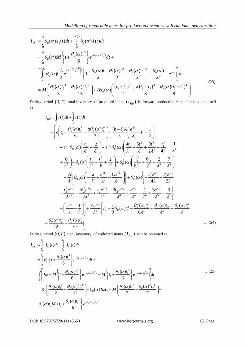
Modelling of repairable items for production inventory with random deterioration
DOI: 10.9790/5728-11145669 www.iosrjournals.org 62 |Page
… (23)
During period ),0( T total inventory of produced items ( )HPI in forward production channel can be obtained
as
1 2
0 0
( ) ( )
t t
HPI I t dt I t dt
1)1(
72
)(
6
)(1
6
1
2
0
3
101
1
teAbtat
tat
42
354)(
2)(
4
1
2
3
1
3
2
1
4
12
032
1
011
tttte
te
tt
4
1
543
1
3
3
12
03
3
1
2
105
726
6)(
2
6)(
6
tttt
24)(
2)(
2222 3
2
4
22
02
2
230
tttt eteteteA
55444
2
2
2
3
2
2
2
2
2 3313
2
3
2
222222
tttttteeetetetet
2
20
2
20
2
3
2
2
03
2022
)()(
6
)()(
3
11 22 ttttt
Aeett
6
)(
12
)( 4
20
5
2
3
0 tt … (24)
During period ),0( T total inventory of collected items ( )HCI can be obtained as
1 2
12
0
22 2
0 0 1
0 0
3( ) 20
0
3 3( ) 2 ( ) 20 0 1
1
0
2 2 4 2 2 4
0 1 0 1 0 2 0 20 2
( ) ( )
( )
6
( ) ( )
6 6
( ) ( ) ( ) ( )( )
2 12 2 12
t t
HC C C
t
t
c
t
t t
c
I I t dt I t dt
tR t e dt
t tBz M t e M t e dt
t t t tR Bzt M
20 1
3( ) 20 1
0 2 1
( )( )
6
ttt M t e
…(25)
3 42
22
0
03 4
0 1 0
0 0
3( ) 20
0
0
( ) 2
2 0 0 0 00 2 2
0
3 2 5
0 2 0 20
( ) ( ) ( ) ( )
( )( )
6
( ) ( ) ( ) ( )( ) 1
2
( ) ( )(
3 15
t tt
DR
t
t
tt t ttt
I tI t dt tI t dt
ttM t e dt
t t eAt e e dt
t tM A
2 3 4
3 4 3 4 0 3 4( ) ( ) ( )( ))
2 3 8
t t t t t t
Modelling of repairable items for production inventory with random deterioration
DOI: 10.9790/5728-11145669 www.iosrjournals.org 63 |Page
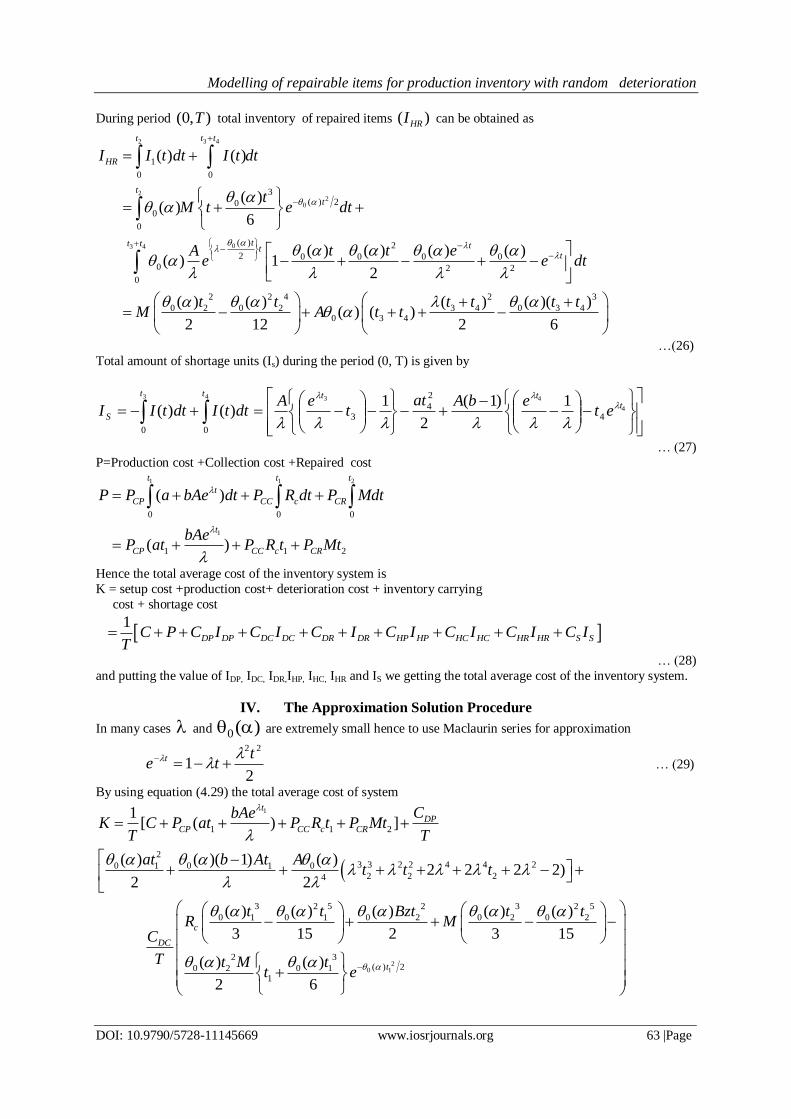
During period ),0( T total inventory of repaired items ( )HRI can be obtained as
3 42
22
0
03 4
1
0 0
3( ) 20
0
0
( ) 2
2 0 0 0 00 2 2
0
2 2 4
0 2 0 2 30 3 4
( ) ( )
( )( )
6
( ) ( ) ( ) ( )( ) 1
2
( ) ( ) (( ) ( )
2 12
t tt
HR
t
t
tt t ttt
I I t dt I t dt
tM t e dt
t t eAe e dt
t t tM A t t
2 3
4 0 3 4) ( )( )
2 6
t t t
…(26)
Total amount of shortage units (Is) during the period (0, T) is given by
43
00
)()(
tt
S dttIdttII
4
43
4
2
43
1)1(
2
1 ttt
etebAat
teA
… (27)
P=Production cost +Collection cost +Repaired cost
1 1 2
1
0 0 0
1 1 2
( )
( )
t t t
t
CP CC c CR
t
CP CC c CR
P P a bAe dt P R dt P Mdt
bAeP at P R t P Mt
Hence the total average cost of the inventory system is
K = setup cost +production cost+ deterioration cost + inventory carrying
cost + shortage cost
1
DP DP DC DC DR DR HP HP HC HC HR HR S SC P C I C I C I C I C I C I C IT
… (28)
and putting the value of IDP, IDC, IDR,IHP, IHC, IHR and IS we getting the total average cost of the inventory system.
IV. The Approximation Solution Procedure
In many cases and )(0 are extremely small hence to use Maclaurin series for approximation
2
122t
te t
… (29)
By using equation (4.29) the total average cost of system
1
1 1 2
23 3 2 2 4 4 20 1 0 1 0
2 2 24
1[ ( ) ]
( ) ( )( 1) ( )2 2 2 2)
2 2
t
DPCP CC c CR
CbAeK C P at P R t P Mt
T T
at b At At t t
2
0 1
3 2 5 2 3 2 5
0 1 0 1 0 2 0 2 0 2
2 3( ) 20 2 0 1
1
( ) ( ) ( ) ( ) ( )
3 15 2 3 15
( ) ( )
2 6
c
DC
t
t t Bzt t tR M
C
T t M tt e
Modelling of repairable items for production inventory with random deterioration
DOI: 10.9790/5728-11145669 www.iosrjournals.org 64 |Page
3 2 5 2 3 4
0 2 0 2 3 4 3 4 0 3 40
( ) ( ) ( ) ( ) ( )( )( )
3 15 2 3 8
DRt t t t t t t tC
M AT
3
0 11
( )
6
HPa tC
atT
3
0
3
102
1
)(2
3
)()1(
Att
Ab
2
0
2
2
20
2
002
)()()()(2
tt
4
2
00
23
202
222
0
2 6
)()(2
3
)(2)(1 t
ttt
A
502
( )
6t
20 1
2 2 4 2 2 4
0 1 0 1 0 2 0 20 2
3( ) 20 1
0 2 1
( ) ( ) ( ) ( )( )
2 12 2 12
( )( )
6
c
HC
t
t t t tR Bzt M
C
T tt M t e
+
2 2 4 2 3
0 2 0 2 3 4 0 3 40 3 4
( ) ( ) ( ) ( )( )( ) ( )
2 12 2 6
HRt t t t t tH
M A t tT
2 2
23 44
( 1)
2 2 2
SC At at A bt
T
… (30)
And
1
1 1 1
23 3 2 2 4 4 20 1 0 1 0
1 1 14
1[ ( ) ( )]
( ) ( )( 1) ( )( ) ( ) 2 2 ( ) 2 2)
2 2
t
DPCP CC c CR
CbAeK C P at P R t P MR t
T T
at b At AR t R t R t
2
0 1
3 2 5 2 3 2 5
0 1 0 1 0 1 0 1 0 1
2 3( ) 20 1 0 1
1
( ) ( ) ( ) ( ) ( ) ( ) ( ) ( )
3 15 2 3 15
( ) ( ) ( )
2 6
c
DC
t
t t BzR t R t R tR M
C
T R t M tt e
2 3
1 4 4 1 4 43 2 5
0 1 0 10 4
0 1 4 4
( ( ) ) ( ( ) )
( ) ( ) ( ) ( ) 2 3( )
3 15 ( )( ( ) )
8
DR
R t t R t t
R t R tCM A
T R t t
3
0 11
( )
6
HPa tC
atT
3
0
3
102
1
)(2
3
)()1(
Att
Ab
2
0 0 0 1 01 2 2 2
( ) ( ) ( ) ( ) ( )( ) 2
R tR t
Modelling of repairable items for production inventory with random deterioration
DOI: 10.9790/5728-11145669 www.iosrjournals.org 65 |Page
3 22 40 0 1 0 0
1 1 12 2
( ) 2 ( ) ( ) 2 ( ) ( )1 ( ) ( ) ( )
3 6
R tAR t R t R t
501
( )(t )
6R
20 1
2 2 4 2 2 4
0 1 0 1 0 1 0 10 2
3( ) 20 1
0 1 1
( ) ( ) ( ) ( ) ( ) ( )( )
2 12 2 12
( )( ) ( )
6
c
HC
t
t t R t R tR Bzt M
C
T tR t M t e
+
2
1 4 42 2 4 1 4 4
0 1 0 10 3
0 1 4 4
( ( ) )( ( ) )
( ) ( ) ( ) ( ) 2( )
2 12 ( )( ( ) )
6
HR
R t tR t t
R t R tHM A
T R t t
2 221 4 44
( ) ( 1)
2 2 2
SC AR t at A bt
T
… (31)
According to equation (30) contain four variables t1, t2, t3 and t4 and these are dependent variable and
related by equation (19) and (20). Also we have K > 0, hence the optimum value of t1 and t4 which minimize
total average cost are the solutions of the equations
01
t
K and 0
4
t
K … (.32)
Provided that these values of t1 satisfy the conditions
02
1
2
t
K, 0
2
4
2
t
K and
22 2 2
2 2
1 4 1 4
. 0K K K
t t t t
Now differentiating (31) with respect to t1 and t4, we get
1
1 1 1 12 2
1
23 3 2 2 4 4 20 1 0 1 0
1 1 14
1
1[ ( ) ( )] 1 ( )
( ) ( )( 1) ( )( ) ( ) 2 2 ( ) 2 2)
2 2
1 ( )
t
DPCP CC c CR
CK bAeC P at P R t P MR t R t
t T T
at b At AR t R t R t
R t
20 1
3 2 5 2 3 2 5
0 1 0 1 0 1 0 1 0 1
2 2 3( ) 20 1 0 1
1
1
( ) ( ) ( ) ( ) ( ) ( ) ( ) ( )
3 15 2 3 15
( ) ( ) ( )
2 6
1 ( )
c
DC
t
t t BzR t R t R tR M
C
T R t M tt e
R t
3 2 5
0 1 0 1
2 3
1 4 4 1 4 412
0 4
0 1 4 4
( ) ( ) ( ) ( )
3 15
( ( ) ) ( ( ) ) 1 ( )2 3
( )( )( ( ) )
8
DR
R t R tM
C R t t R t t R tT
AR t t
Modelling of repairable items for production inventory with random deterioration
DOI: 10.9790/5728-11145669 www.iosrjournals.org 66 |Page
3
0 112
( )
6
HPa tC
atT
3
0
3
102
1
)(2
3
)()1(
Att
Ab
2
0 0 0 1 01 2 2 2
( ) ( ) ( ) ( ) ( )( ) 2
R tR t
3 22 40 0 1 0 0
1 1 12 2
( ) 2 ( ) ( ) 2 ( ) ( )1 ( ) ( ) ( )
3 6
R tAR t R t R t
501 1
( )( ) 1 ( )
6R t R t
20 1
2 2 4
0 1 0 10 1
2 2 4
0 1 0 112
3( ) 20 1
0 2 1
( ) ( )( ) ( )
2 12
( ) ( ) ( ) ( )1 ( )
2 12
( )( )
6
c
HC
t
t tR BzR t
C R t R tM R t
T
tt M t e
2
1 4 42 2 4 1 4 4
0 1 0 10 12 3
0 1 4 4
( ( ) )( ( ) )
( ) ( ) ( ) ( ) 2( ) 1 ( )
2 12 ( )( ( ) )
6
HR
R t tR t t
R t R tHM A R t
T R t t
2 2
21 4 44 12
( ) ( 1)1 ( )
2 2 2
SC AR t at A bt R t
T
1
1
3 2 2 40 00 1 1 1 1 1 14
1[ ( ) ( )]
( )( 1) ( )( ) 3 ( ) ( ) 2 ( ) ( ) 2 ( )
2
t DPCP CC c CR
CP a bAe P R P MR t
T T
b A Aat R t R t R t R t R t
2 20 1 0 1
2 2 4
0 1 0 1 0 1 1
2 2 4
0 1 1 0 1 1
3 2 2( ) 2 ( ) 20 1 1 0 1 0 1 0 1
1
2
0
3 ( ) ( ) 2 ( ) ( ) ( )
3 3 2
3 ( ) ( ) ( ) ( ) ( ) ( )
3 3
2 ( ) ( ) ( ) ( ) ( ) ( ) ( )1
2 6 2 2
( )
c
DC
t t
t t BzR t R tR
R t R t R t R tM
C
T R t R t M t R t M tt e e
2
0 1
2 3( ) 21 1 0 1
1
t ( ) ( )
2 6
tR t M tt e
2 2 4
0 1 1 0 1 13 ( ) ( ) ( ) ( ) ( ) ( )
3 3
DRR t R t R t R tC
MT
Modelling of repairable items for production inventory with random deterioration
DOI: 10.9790/5728-11145669 www.iosrjournals.org 67 |Page
2
0 1( )
2
HPa tC
aT
0 1
1
( )( 1)2
1
tb A At
0 0 0 1 11 2 2
( ) ( ) 2 ( ) ( ) ( )( ) 2
R t R tR t
2 230 0 1 1 0 0
1 1 1 1 12 2
( ) 2 ( ) ( ) ( ) 2 ( ) ( )1 ( ) 2 ( ) ( ) 2 ( ) ( )
1 3
R t R tAR t R t R t R t R t
401 1
5 ( )(t ) ( )
6R R t
2 20 1 0 1
2 3 2 3
0 1 0 1 0 1 1 0 10 1
3 2( ) 2 ( ) 20 1 0 1
0 1 1 0 1
2 2
0 1 1 0 1
2 ( ) ( ) 2 ( ) ( ) ( ) ( ) ( )( ) ( )
2 3 2 3
( ) ( )( ) ( ) ( ) ( ) 1
6 2
( ) t ( ) ( )1
2
c
t tHC
t t R t R t R tR BzR t M
C t tR t M t e R t M e
T
R t M t
20 1( ) 2t
e
+
2 3
0 1 1 0 1 12 ( ) ( ) ( ) ( ) ( ) ( )0
2 3
HRR t R t R t R tH
MT
… (33)
1
1 1 1 1 42 2
4
2
0 1 0 1 0
4
1 4
3 3 2 2 4 4 2
1 1 1
1[ ( ) ( )] 1 ( )
( ) ( )( 1) ( )
2 2 1 ( )
( ) ( ) 2 2 ( ) 2 2)
t
DPCP CC c CR
CK bAeC P at P R t P MR t R t
t T T
at b At A
R t
R t R t R t
20 1
3 2 5 2
0 1 0 1 0 1
3 2 5
0 1 0 11 42
2 3( ) 20 1 0 1
1
( ) ( ) ( ) ( )
3 15 2
( ) ( ) ( ) ( )1 ( )
3 15
( ) ( ) ( )
2 6
c
DC
t
t t BzR tR
C R t R tM R t
T
R t M tt e
3 2 5
0 1 0 1
2 3
1 4 4 1 4 41 42
0 4
0 1 4 4
( ) ( ) ( ) ( )
3 15
( ( ) ) ( ( ) ) 1 ( )2 3
( )( )( ( ) )
8
DR
R t R tM
C R t t R t t R tT
AR t t
Modelling of repairable items for production inventory with random deterioration
DOI: 10.9790/5728-11145669 www.iosrjournals.org 68 |Page
3
0 112
( )
6
HPa tC
atT
3
0
3
102
1
)(2
3
)()1(
Att
Ab
2
0 0 0 1 01 2 2 2
( ) ( ) ( ) ( ) ( )( ) 2
R tR t
3 22 40 0 1 0 0
1 1 12 2
( ) 2 ( ) ( ) 2 ( ) ( )1 ( ) ( ) ( )
3 6
R tAR t R t R t
501 1 4
( )( ) 1 ( )
6R t R t
20 1
2 2 4 2 2 4
0 1 0 1 0 1 0 10 1
2 3( ) 20 1
0 2 1
1 4
( ) ( ) ( ) ( ) ( ) ( )( ) ( )
2 12 2 12
( )( )
6
1 ( )
c
HC
t
t t R t R tR BzR t M
C
T tt M t e
R t
2 2 4
0 1 0 1
2
1 4 41 42 1 4 4
0 3
0 1 4 4
( ) ( ) ( ) ( )
2 12
( ( ) ) 1 ( )( ( ) )2
( )( )( ( ) )
6
HR
R t R tM
H R t t R tR t tT
AR t t
2 2
21 4 44 1 42
( ) ( 1)1 ( )
2 2 2
SC AR t at A bt R t
T
2
1 4 1 4 1 4 4 1 4
0 3
0 1 4 4 1 4
( ( ) )( ( ) 1) ( ( ) ) ( ( ) 1)
1 1( )
( )( ( ) ) ( ( ) 1)
2
DR
R t t R t R t t R t
CA
T R t t R t
+
2
0 1 4 4 1 41 4 4 1 40 1 4
( )( ( ) ) ( ( ) 1)( ( ) )( ( ) 1)( ) ( ( ) 1)
1 2
HRR t t R tH R t t R t
A R tT
1 4 1 4 4 4( ) ( ) ( 1) 0SCAR t R t at A b t
T
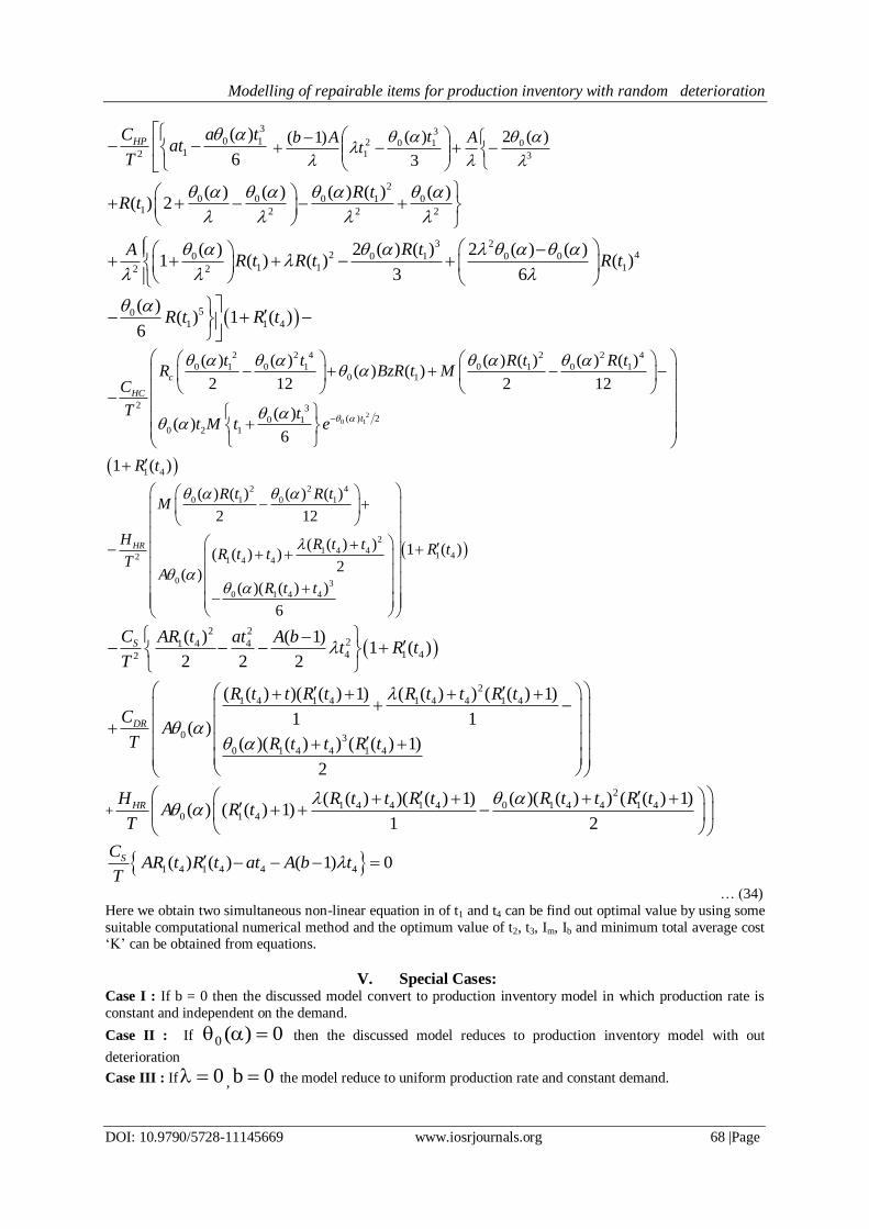
… (34)
Here we obtain two simultaneous non-linear equation in of t1 and t4 can be find out optimal value by using some
suitable computational numerical method and the optimum value of t2, t3, Im, Ib and minimum total average cost „K‟ can be obtained from equations.
V. Special Cases: Case I : If b = 0 then the discussed model convert to production inventory model in which production rate is
constant and independent on the demand.
Case II : If 0)(0 then the discussed model reduces to production inventory model with out
deterioration
Case III : If 0 , 0b the model reduce to uniform production rate and constant demand.
Modelling of repairable items for production inventory with random deterioration
DOI: 10.9790/5728-11145669 www.iosrjournals.org 69 |Page
VI. Conclusion In the proposed model a production inventory model is formulated for random deteriorating item with a
increasing market demand rate with time and production rate is dependent on the demand. Result in this study
can provide a valuable reference for decision markers in planning the production and controlling the inventory.
The model proposed here in is resolved by using maclaurin series and cost minimization technique is used to get
the approximate expression for total average cost and other parameters & some special cases of model are also
discussed. We derive an expressions for different cost associated in the model. We derive equations, solution of
these equations gives the optimal cycle and optimal cost of repairable items. A future study will incorporate
more realistic assumption in the proposed model.
References [1]. Alamri, A.A. (2010). Theory and methodology on the global optimal solution to a Reverse logistics inventory model for
deteriorating items and time varying rates. Computer & Industrial Engineering,(60), 236-247.
[2]. Balkhi, Z. T. and Benkherouf, L. (1996 b)On the optimal replenishment schedule for an inventoy system with
deteriorating items and time varying demand and production rates.Computers & Industrial Engineering, 30 ; 823-829..
[3]. Bhunia, A. K. and Maiti , M. (1998) A two warehouse inventory model for deteriorating items with a linear trend in
demand and shortages.Jour of Opl. Res. Soc., 49 : 287-292.
[4]. Chang, H. J . and Dye, C. Y. (1999) An EOQ model for deteriorating items with time varying demand and partial
backlogging.J o ur , o f O pl . Res . So c . , 50 : 117 6 -11 82 .
[5]. Chung, C. J., & Wee, H. M. (2011). Short life-cycle deteriorating product remanufacturing in a green supply chain inventory
control system. International Journal of Production Economics, 129(1), 195-203.
[6]. Covert, R.P., and Philip, G.C.,( 1973), An EOQ Model for Item with Weibull Distribution Deterioration, AIIE Transactions, 5,
(4), 323-326,
[7]. Dobos, I., & Richter, K. (2003), A production/recycling model with stationary demand and return rates.Central European journal
of Operations Research, 11(1), 35-46.
[8]. Dobos, I., & Richter, K. (2004), An extended production/recycling model with stationary demand and return rates. International
Journal of production Economics, 90(3), 311-323.
[9]. Dobos, I., & Richter, K. (2006), A production/recycling model with quality considerations. International Journal of Production
Economics, 104(2), 571-579.
[10]. El Saadany A. M. A., & Jaber M. Y. (2010)., A production/ remanufacturing inventory model with price and quality dependant
return rate. Computers and Industrial Engineering, 58(3), 352–362.
[11]. Ghare, P.M., and Schrader, G.F.,(1963), A Model for An Exponentially Decaying Inventory, The Journal of Industrial
Engineering, 14, (5), 238-243.
[12]. Goswami, A and Chaudhuri, K. S. (1991) EOQ model for an inventory with a linear trend in demand and finite rate of
replenishment considering shortages.int . J our. Syst ScL, 22, 181-187.
[13]. Konstantaras, I., & Skouri, K. (2010), Lot sizing for a single product recovery system with variable set up numbers. European
Journal of Operations Research, 203(2), 326-335.
[14]. Perumal, V. and Arivarignan, G. (2002)A production inventory model with two rates of production and
backorders.Int. Jo ur of Mgt. & Syst ., 18 (1) : 109 -119.
[15]. Pyke, D. (1990 )“Priority Repair and Dispatch Policies for Reparable-Item Logistics Systems.”Naval Research Logistics v37 n1 1-
30 Feb.
[16]. Raafat, F., Wolfe, P.M. and Eldin, H.K. An Inventory Model for Deteriorating Item, Computers & Industrial Engineering, 20,
(1), 89-94, 1991.
[17]. Richter, K, (1996b). The extended EOQ repair and waste disposal model. International Journal of Production Economics, 45(1-3),
443-447.
[18]. Richter, K. (1996), The EOQ repair and waste disposal model with variable setup numbers. European Journal of Operational
Research, 95(2), 313-324.
[19]. Richter, K., & Dobos, I. (1999). Analysis of the EOQ repair and waste disposal model with integer set up numbers. International
journal of production economics, 59(1-3), 463-467.
[20]. Schrady, D.A. (1967). A deterministic inventory model for repairable items. Naval Research Logistics Quarterly, 14, 391–398.
[21]. Teng, J. T. & Chang, C. T. (2005). Economic production quantity models for deteriorating items with price and stock-dependent
demand. Computational Operations Research, 32 (2), 297-308.
[22]. Teng, J . T. (1996) A deterministic replenishment model with linear trend in demand. Opns. Res. Lett . 19 : 33-41.