Licentiate DissertationStructural

Mechanics

KRISTIAN STÅLNE

MODELLING OF STIFFNESS ANDHYGROEXPANSION OF WOODFIBRE COMPOSITES

Detta är en tom sida!

Copyright © 2001 by Structural Mechanics, LTH, Sweden.Printed by KFS I Lund AB, Lund, Sweden, November 2001.

For information, address:

Division of Structural Mechanics, LTH, Lund University, Box 118, SE-221 00 Lund, Sweden.Homepage: http://www.byggmek.lth.se

Structural Mechanics

ISRN LUTVDG/TVSM--01/3061--SE (1-92)ISSN 0281-6679

MODELLING OF STIFFNESS AND

HYGROEXPANSION OF WOOD

FIBRE COMPOSITES

KRISTIAN STÅLNE

PREFACE

The work presented in this dissertation was carried out during the period 1998-

2001 at the Division of Structural Mechanics, Department of Building and Envi-

ronmental Technology, Lund University, Sweden. The �nancial support by the

Swedish Foundation for Strategical Research (SSF) programme "Wood Tech-

nology" is gratefully acknowledged.

I would like to thank my supervisor, Prof. Per Johan Gustafsson, for his pa-

tience, encouragement, for always having time for discussions and for being a

very skilful supervisor. I also would like to thank Kent, Erik, Peter, Jonas,

Per-Anders and the rest of the sta� at the structural mechanics division for

always helping me when I am in con ict with my computer and for making this

working environment very pleasant.

Special thanks go to Dr. Dennis Rasmusson and Dr. Bijan Adl Zarrabi for good

collaboration and for the practical training period I spent at Perstorp AB and

to Dr. H�akan Wernersson at Pergo AB for valuble discussions.

I �nally would like to thank my family and friends and the rest of my "pack"

consisting of Jenny and Ruben for all support and encouragement.

Lund, November 2001

Kristian St�alne

1

CONTENTS

Summary of Papers 1-4

Introduction

Paper 1 K. St�alne (2001), Review of Analytical Models for Sti�ness and Hy-

groexpansion of Composite Materials, Report TVSM-7133, Division

of Structural Mechanics, Lund University.

Paper 2 K. St�alne (1999), Analysis of Fibre Composite Models for Sti�ness

and Hygroexpansion, Report TVSM-7127, Division of Structural Me-

chanics, Lund University.

Paper 3 K. St�alne and P. J. Gustafsson (2000) A 3D Model for Analysis of

Sti�ness and Hygroexpansion Properties of Fibre Composite Materi-

als, accepted for publication in ASCE's Journal of Engineering Me-

chanics.

Paper 4 K. St�alne and P. J. Gustafsson (2001) A 3D Finite Element Fibre

Network Model for Composite Material Sti�ness and Hygroexpansion

Analysis, to be submitted to the Journal of Composite Materials,

Technomic Publishing Co., Inc.

2

SUMMARY OF PAPERS 1-4

Paper 1 The �eld of research involving the analytical modelling of the sti�-

ness and hygroexpansion of composite material is reviewed. This

paper can be regarded as an introduction to the area of the mechan-

ics of composite materials in general and to wood �bre composites

in particular. The most important models, such as the Reuss and

Voigt bounds and the Halpin-Tsai, are described, along with their

advantages and limitations. The report also contains examples of

calculations made for various models, allowing them to be compared.

Paper 2 In this paper, coordinate transformations of the stresses, strains and

sti�ness of composite materials are described. A new method for

interpolating between the extremes of homogeneous strain and ho-

mogeneous stress for calculating the sti�ness matrix of composites

is introduced. This new interpolation method is shown by use of

advanced matrix theory, to be coordinate independent.

3

Paper 3 A 3D analytical model for sti�ness and hygroexpansion is presented.

The model involves two steps. The �rst step is the homogenisation

of a structure composed of a single wood �bre coated by a layer of

matrix material. The second step is the integration of the various

�bre orientations involving a linear and an exponential interpolation

between an extreme case of homogenous strain and an extreme case

of homogenous stress. A comparison is made between the prediction

as modelled and measurement data for sti�ness, Poisson's ratio and

hygroexpansion. The matrix material is assumed to have isotropic

properties, whereas the �bres and the particle material can have ar-

bitrary orthotropic properties. The model can be used for all volume

fractions and is also valid for particle composites.

Paper 4 This paper presents a 3D numerical model for the sti�ness and hy-

groexpansion properties of wood �bre composite materials. The mi-

crostructure of a composite composed of a number of �bres is mod-

elled by use of a �bre geometry preprocessor. The model is employed

for analysing the mechanical behaviour of wood �bre composites that

have �bre network geometries. Results obtained by use of the model

are compared with results based on the analytical model presented

in paper 3 and with various test results.

4

INTRODUCTION

1 Background

Wood composite materials are gaining in popularity, both for environmental

reasons and because of their high performance-to-cost ratio. A matter that is

often a drawback, however, when wood products are employed is their shape

instability when subjected to a change or a gradient in moisture content. This

is of considerable importance for both solid timber and wood-based composite

materials. At the same time, there are important di�erences between compos-

ites and solid timber. One of these is the greater variability found in a timber

structural member due to knots, grain deviations, etc, making predictions of

shape instability and other properties uncertain. Another di�erence is in the

possibility of designing a composite for uses of speci�c types. Wood composite

materials can be designed to be of very di�ering properties in terms of strength

and sti�ness, product dimensions, heat insulation properties, sound mu�ing,

durability, shape stability etc.

The design or improvement of a composite material, whether it already exists

or is only being considered for possible manufacture, is very much facilitated

by access to some form of calculation model that enables analysis and predic-

tions of the performance of the material to be made. Access to a general and

accurate tool for analysing and predicting the load and the moisture induced de-

formations of a composite material would certainly be of great value and would

promote the use of wood composites.

The orthotropic and moisture-sensitive nature of wood materials has led to dif-

�culties in modelling their mechanical behaviour. Even in the case of linear

elasticity there are nine independent sti�ness constants and three independent

hygroexpansion parameters that need to be taken account of. In modelling

wood composites, one has to also take the structure of the material, including

the shape of the wood �bres or of the wood particle, the matrix properties and

the �bre-matrix interaction, into consideration. Studying the literature on com-

posite material modelling, it is evident that the more complicated a composite

is, the less interest there is in modelling it.

The possibilities of �nite element analysis have been increased very much by

developments in computer performance. It is possible now to analyse complex

structures by use of fairly detailed models. Finite element analysis is used to-

day for the continuum modelling of moisture-induced deformations of solid wood

members [3]. The detailed FE-modelling of wood �bres and of the heterogeneous

5

structure of small pieces of wood has been used to analyse the in uence of the

microstructure of wood on its global homogenised properties [2]. However, even

if the performance of today's computers is impressive, in the foreseeable future

it would still appear possible to model only very small volumes of a heteroge-

neous composite material structure. Analytical composite material modelling is

generally, more convenient to apply, but in some cases the results are more of

an approximate character.

2 Scope of the Present Work

The work presented in this licentiate dissertation is the �rst part of a PhD

project aiming at developing a computational tool allowing the global deforma-

tion properties of wood �bres or of particle composite materials and products to

in theory be predicted from the known properties of their constituents, as well

as the structure of the composite material. Achieving this overall goal involves

two basic steps. The �rst step is to create a model of the microstructure of wood

�bre composite materials, making it possible to analyse the global deformations

of small pieces of the composite material when exposed to homogeneous states of

climate and to mechanical load. This concerns the rate- and time-independent

performance of the materials, as presented in this report. Numerical examples

and experimental veri�cations of high pressure laminates, HPL, used in such

applications as ooring [1], are presented in Figure 1.

Figure 1: HPL oor under hygroexpansion.

The present licentiate dissertation is composed of four papers. In paper 1 the

research area of composite material sti�ness and of hygroexpansion modelling

is reviewed. Paper 2 deals with coordinate transformations, an analytical in-

terpolation method being introduced and investigated thoroughly. The method

described is used in paper 3 in connection with the presentation of a complete

analytical homogenisation model. Finally, in paper 4, a �nite element model

of an HPL is described and is compared with results obtained by use of this

6

analytical model and with various test results.

3 Future Work

The major part of the second step in the PhD project will be to create a con-

tinuum mechanics model of the deformation properties of a composite material.

The parameter values for use in this model are to be obtained by use of a

numerical microstructure model or of an analytical composite material model.

Time-dependent properties such as creep and mechanosorption will also be im-

plemented �rst in a micromechanics model and then in a continuum mechanics

model. By means of this material model and of the �nite element method it will

be possible to calculate the moisture-induced deformations of products made of

wood composites when exposed to various loading conditions and climatic con-

ditions.

References

[1] Adl Zarrabi, B. (1998). Hygro-Elastic Deformation of High Pressure Lami-

nates. Doctoral thesis, Division of Building Material, Chalmers University

of Technology, Sweden

[2] Persson, K. (2001). Micromechanical modelling of wood and �bre proper-

ties. Doctoral thesis, Division of Structural Mechanics, Lund University,

Sweden.

[3] Ormarsson, S. (1999). Numerical Analysis of Moisture-Related Distor-

tions in Sawn Timber. Doctoral Thesis, Division of Structural Mechanics,

Chalmers University of Technology, Sweden.

7

Review of Analytical Models for

Sti�ness and Hygroexpansion

of Composite Materials

Kristian St�alne

Division of Structural Mechanics

Lund University, Sweden

I

1 Introduction

1.1 Contents of the report

This report is an overview of analytical models for sti�ness and hygroexpansion

analysis of composite materials. The most important linear elastic models are

presented and discussed. In the �rst section di�erent composite materials are

de�ned and described, with emphasis being placed on wood �bre composites.

The concept of homogenisation, the reason for homogenising a composite ma-

terial and ways of doing so are then discussed. Important advances recently in

the �eld of composite homogenisation are described brie y. The models most

frequently used for the homogenisation of the sti�nesses are then examined,

the important issue of calculating hygroexpansion properties being taken up.

Finally examples are provided of sti�ness and hygroexpansion calculations for

a high pressure laminate. References is also made in this report to various

other useful and comprehensive reviews of research in the area of the composite

material mechanics.

1.2 De�nition of a composite material

A composite material is created when two or more materials are mixed in or-

der to achieve di�erent properties than those of its constituents. The regions

occupied by the seperate constituents are considered as being homogeneous

continua and are commonly assumed to be bonded together �rmly at the re-

spective interfaces. The main advantage of using a composite material is that

it can be tailor-made for a particular application. By adding �bres aligned in

one preferred direction, the material can be made sti�er and stronger in that

direction. This makes it possible to achieve light but sti� materials. Di�erent

types of composite materials can be distinguished on the basis of their function

and of the structural geometry of the material: particle composites, �bre com-

posites, laminate composites and composites with irregular geometry, according

to Figure 1 which is taken from [30]. The particle composite most frequently

employed is concrete. There, cement is mixed with sand and small stones to

produce a material that is cheaper and has improved properties, such as having

lesser moisture-induced strains. Reinforcing concrete with steel rods provides

it a high degree of strength, also when under tension. Concrete can also be

reinforced with steel or glass �bres, making it a �bre composite as well [25].

Laminate composites are created by placing thin isotropic or anisotropic plates

or laminas, on top each other, making it easier to control the sti�ness.

Fibre composites are often classi�ed by the �bre length and the �bre orienta-

tion distribution. Fibres can either be placed in one direction, be arranged in a

weave, or arranged in accordance with some continuous orientation distribution

1

Figure 1: a) particle composites, b) �bre composites, c) laminate composites and

d) composites with irregular geometry.

function. Fibre materials commonly used here are glass, carbon, aramid and

wood. The surrounding phase, or matrix, is often some polymer such as epoxy

or polyester.

1.3 Wood composite materials

Natural composite materials containing �bres or particles obtained from wood

or from plants such as ax and hemp are gaining in popularity, both of environ-

mental reasons and due to their high performance and their low cost and low

weight. Wood-based composites are commonly created either by joining wood

particles by some adhesive, by mixing wood our with a thermoplastic [33] or

by impregnating paper with a resin. An advantage of wood composites as com-

pared with solid wood is that they are more homogenous and are without such

weaknesses as knots. Such engineering wood products as glulam and laminated

veneer lumber, on the other hand, are not considered as composite materials,

whereas paper and �bre boards, which have a very low matrix phase volume

fraction, sometimes are referred to as being composite materials.

High pressure laminates, or HPL, are wood �bre composites which have under-

gone a strong development during the last decade or so. They are composed

of layers of craft paper impregnated with phenolic or melamine resin and cured

under high pressure and at high temperature [3]. Although consisting of layers

of di�ering sti�ness, HPL is considered here as a �bre composite and not as a

laminate composite. One problem in connection both with HPL and with all

other wood composites, is that of shape instability when changes in moisture

2

content occur. This makes it important to have a good understanding of how

to predict and control the sti�ness and hygroexpansion properties of HPL.

2 Elastic Properties of Composite Materials

2.1 Homogenisation

Composite materials have gained in popularity in various industrial applications

such as in the automotive, the space and the building industries. In all appli-

cations there is a need of simulating the mechanical behaviour of elements or

of entire structures. Although computer simulation capacity is increasing, it

will hardly be possible to model every single �bre, such as in an airplane for

example. The only practical approach to simulation is to regard a composite

material as being continuous and homogeneous. Since micro-scale properties

such as �bre sti�ness and orientation are decisive for the global behaviour of

the material, homogenisation is very important.

Homogenisation also allowes one to calculate such e�ective properties as those

of sti�ness and hygroexpansion when the corresponding properties of the con-

stituents as well as information concerning the geometry of the material, such as

the direction in which the �bres are aligned, are known [34, 29]. A number of as-

sumptions need to be made: that no chemical interaction between the di�erent

phases occurs, that the phases are homogeneous and distinctly separated, and

that there is statistical homogeneity allowing one to de�ne a volume element

which is representative of the structure as a whole. In order to calculate the

sti�ness and the hygroexpansion of a composite made up of two linear elastic

materials, one needs information on the sti�ness matrices of the constituents,

Df and Dm, the hygroexpansion coe�cients vectors, �f and �m, the volume

fractions, Vf and Vm, and the shape as well as the orientation distribution of

the �bres or particles.

Homogenisation is achieved by analysing a representative volume element, RVE.

In its structure and composition the RVE is typical for the composite as a whole.

E�ective mechanical properties are calculated from the response of the RVE

when exposed to a prescribed boundary force or deformation. When the e�ec-

tive hygroexpansion coe�cients of the composites are calculated, which is done

in a way directly analogous to calculation of the thermal expansion coe�cients,

the prescribed boundary conditions can be obtained by use of a prescribed

change in moisture content.

The choice of boundary conditions in uences the results, for example, when a

3

Figure 2: A RVE exposed to a force in one direction.

prescribed displacement at the boundary is assumed, the sti�ness of the RVE

is overestimated, due to the extra constraint. The assumption of a prescribed

traction also results in the sti�ness being underestimated. There is the possi-

bility of using cyclic boundary conditions [20]. This requires use of a periodic

geometry for the RVE, such as that of a �bre that passes through a boundary

having the same inclination on the opposite side.

3 Literature Concerning Homogenisation

Methods

Use of adequate methods for homogenisation is very important in simulating

structures made of composite materials, since an error in the properties of the

composite material results in an equally large error in the structural simulation,

irrespective of how accurate the simulation may be. The greatest di�culty in

homogenising materials is often that of obtaining reliable material data. For

wood particles, there are nine sti�ness components and three hygroexpansion

components that need to be known or be estimated. If the properties of the

constituents are known, it is the quality of the homogenisation model which

4

is decisive for the accuracy and reliability of predicting the properties of the

composite material.

In working with composite homogenisation models, one is in good company,

the �rst contributions to this research area having been made in the late 19th

century by such scientists as Maxwell, Boltzmann and Einstein [34]. The most

important and general models are the Voigt approximation (1889) [1] and the

Reuss approximation (1929) [1], based on the assumption of homogeneous strain

and of homogeneous stress, respectively. Hill (1952) [22], who showed that these

two approximations are in fact boundaries for the overall sti�ness components

regardless of the geometry of the constituents, formulated a number of funda-

mental theoretical principles here [21]. The development of mathematical and,

to various degrees, empirical models increased in the early 1960s when the tech-

nical importance of composite materials came clear.

Models for unidirectional �bre composites were created, such as the Halpin-Tsai

equations (1963) [14] which are probably those most frequently employed. A

number of methods for calculating transverse sti�ness of composites containing

�bres of di�ering geometries, such as the method of Hashin-Shtrikman bounds

(1965) [17, 18], were derived.

Models for particle composites are usually derived by considering a single parti-

cle in an e�ective medium of some sort. Models of this type include the Eshelby

equivalent inclusion method (1957) [11] for elliptical particles, the Mori-Tanaka

theory (1973) [31], the self-consistent scheme (1965) and the generalized self-

consistent scheme [15]. All existing models for particle composites assume the

particles to be isotropic. A directional average for the particle phases can also

be obtained, however without any great di�culty. Other approaches to the anal-

ysis of e�ective sti�ness have been developed by Hashin [19, 16], Luciano [28]

and Chen [7]. Theoretical analyse of the e�ect of the length and the orientation

of the �bre have been carried out by Fu et al. [12], Sayers [37], Munson-McGee

et al. [32] and Dunn et al. [10]. Stresses in the �bres and in the matrix have

been investigated by Carman et al. [6].

Homogenisation of the hygroexpansion properties, which in mathematical terms

is identical with thermal expansion, has become of lesser interest. Certain fun-

damental results for anisotropic composites have been derived by Levin [27], and

by Rosen and Hashin [36, 19]. Camacho et al. [5] have performed 3D modelling

and compared the results with measurement data.

Comprehensive reviews of composite material modelling are provided by Dunn

5

et al. [10] who present a long list of additional references; by Tucker [40] who

compares a number of analytical models for unidirectional short �bre compos-

ites involving �nite element calculations; and by Hashin [15], whose review is

best, containing a very informative and critical review of the �eld of composite

material analysis as a whole.

It would appear that most models concern rather specialized cases, such as

those of isotropy, of long unidirectional �bres, or of circular or hexagonal �bre

geometries, the one as accurate as the other. Most models provide estimates

of elastic, transverse and longitudinal moduli [26]. Obviously, a great deal of

work needs to be done to investigate more complicated composites such as those

with anisotropic constituents or with �bre-to-�bre interactions, or that are non-

unidirectional, such as HPL.

Models used in many industrial applications, such as the Halpin-Tsai equations

or the rule of mixture, often su�ce for estimating single e�ective properties

such as longitudinal sti�ness, but tend to be inadequate or inappropriate for

estimating the other sti�ness and hygroexpansion components needed, such as

for the indata in the case of �nite element analysis.

4 Models of Sti�ness

4.1 The Voigt and the Reuss models

The simplest forms of homogenisation involve assuming either that the strain

�eld or the stress �eld is uniform. The �rst of these two assumptions requiers

adding the stresses weighted by the respective volume fractions, Vi, which yields

to the expression for composite material sti�ness matrices

D� = V1D1 + V2D2 (1)

that Voigt [1] introduced, called the Voigt approximation or the rule of mix-

ture, ROM. The asterisk indicates the e�ective property to be intended. Other

designations of this approach, which is probably the homogenisation method

most frequently employed, are the parallel coupling model and the homogeneous

strain model. The assumption of a uniform strain �eld entails the tractions at

the phase boundaries not being in equilibrium.

The approximation given by the assumption of a homogeneous stress �eld was

introduced by Reuss [1]. It leads to the analogous expression

6

C� = V1C1 + V2C2 (2)

where C = D�1 is the compliance matrix. This is called the Reuss approxi-

mation or the series-coupling model. The strains under uniform stress are such

that the deformations of the inclusions and the matrix are not compatible. The

Voigt and the Reuss approximations are the most important ones since they con-

stitute the bounds for all of the components in D� of any composite material,

regardless of its geometry, as determined by Hill [22] on the basis of rigorous

calculations. These bounds are very easy to use, but if the properties of the

constituents di�er too much the provide too large an interval to be of practical

use.

4.2 Interpolation between the Voigt and Reuss models

The one dimensional versions of parallel and of serial coupling can be written

as a single equation with a parameter � [24] for a scalar sti�ness parameter,

E� = (V1E�1 + V2E

�2 )

1=�(3)

where � = 1 is the case of one-dimensional parallel coupling and � = �1 that

of the serial coupling. By giving the variable � a particular value �1 < � < 1

an interpolation is achieved. For � = 0 the equation can be written as E� =

V E1

1 � V E2

2 . Observe that � = 1 corresponds to the arithmetic mean, � = �1 to

the harmonic mean and � = 0 to the geometric mean of the sti�nesses.

This interpolation can also be extended to the two- and three dimensional case,

as shown by St�alne [38]

D� = (V1D

�1 + V2D

�2 )

1=�(4)

The interpolation can be performed on an integral as well, as will be shown in

the section "Composites containing arbitrarily oriented �bres".

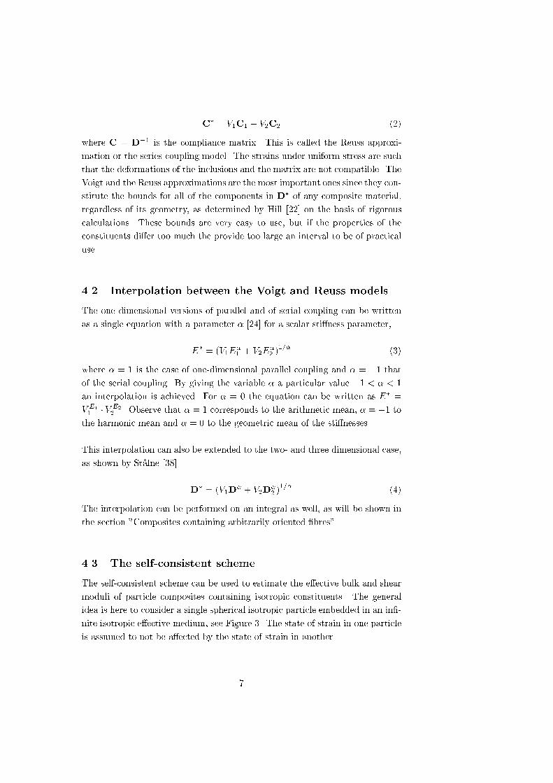
4.3 The self-consistent scheme

The self-consistent scheme can be used to estimate the e�ective bulk and shear

moduli of particle composites containing isotropic constituents. The general

idea is here to consider a single spherical isotropic particle embedded in an in�-

nite isotropic e�ective medium, see Figure 3. The state of strain in one particle

is assumed to not be a�ected by the state of strain in another.

7

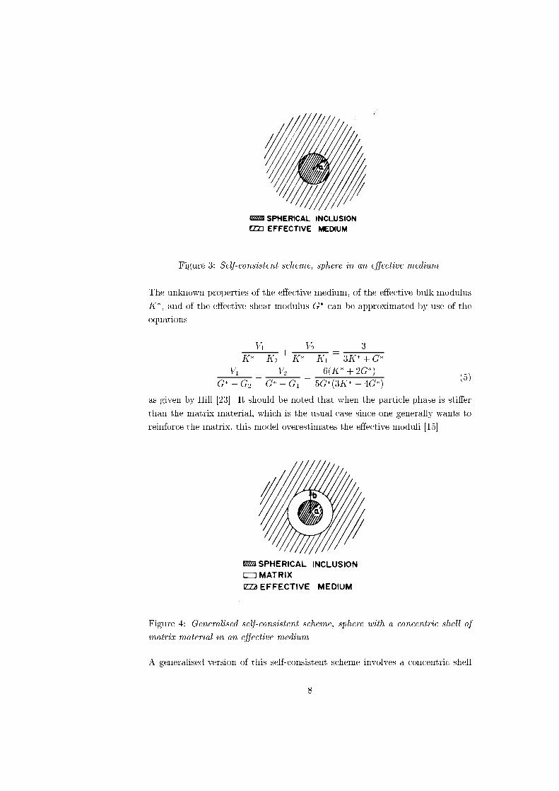
Figure 3: Self-consistent scheme, sphere in an e�ective medium.

The unknown properties of the e�ective medium, of the e�ective bulk modulus

K�, and of the e�ective shear modulus G� can be approximated by use of the

equations

V1K� �K2

+V2

K� �K1=

3

3K� +G�

V1G� �G2

+V2

G� �G1=

6(K� + 2G�)

5G�(3K� + 4G�)(5)

as given by Hill [23]. It should be noted that when the particle phase is sti�er

than the matrix material, which is the usual case since one generally wants to

reinforce the matrix, this model overestimates the e�ective moduli [15].

Figure 4: Generalised self-consistent scheme, sphere with a concentric shell of

matrix material in an e�ective medium.

A generalised version of this self-consistent scheme involves a concentric shell

8

of matrix material surrounding the spherical particle, Figure 4. This version is

considered more realistic, but is also far more complicated and has no explicit

solution.

4.4 The Halpin-Tsai equations

The most popular model for predicting the sti�ness of short unidirectional �bre

composites is that involving the Halpin-Tsai equations [14]. These were derived

from approximations of Hill's generalised self-consistent model [23]. In dealing

with the composite, each �bre is assumed to behave as though it were surrounded

by a pure matrix cylinder, a body with the properties of the composite lying

outside the cylinder. The constituents are considered to be homogeneous and

to be transversely isotropic in the direction of the �bre. The composite sti�ness

in the longitudinal direction is given by

E�L = Em1 + ��Vf1� �Vf

� =Ef �Em

Ef + �Em(6)

where Em is the matrix material sti�ness and � = 2a=b is a factor of the geome-

try controlled by the �bre length-thickness ratio a=b, where a is the �bre length

and b the �bre thickness as shown in Figure 5.

Figure 5: Fibres of length a and width b in a matrix material.

9

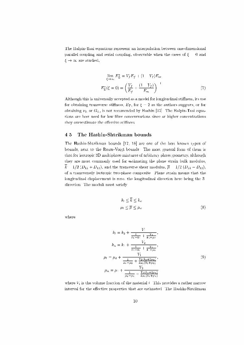
The Halpin-Tsai equations represent an interpolation between one-dimensional

parallel coupling and serial coupling, observable when the cases of � = 0 and

� !1 are studied,

lim�!1

E�L = VfEf + (1� Vf )Em

E�L(� = 0) =

�VfEf

+(1� Vf )

Em

��1

(7)

Although this is universally accepted as a model for longitudinal sti�ness, its use

for obtaining transverse sti�ness, ET , for � = 2 as the authors suggests, or for

obtaining �L or GL, is not recomended by Hashin [15]. The Halpin-Tsai equa-

tions are best used for low �bre concentrations since at higher concentrations

they overestimate the e�ective sti�ness.

4.5 The Hashin-Shtrikman bounds

The Hashin-Shtrikman bounds [17, 18] are one of the best known types of

bounds, next to the Reuss-Voigt bounds. The most general form of them is

that for isotropic 3D multiphase mixtures of arbitrary phase geometry, although

they are most commonly used for estimating the plane strain bulk modulus,

k = 1=2 (D11 +D12), and the transverse shear modulus, � = 1=2 (D11 �D12),

of a transversely isotropic two-phase composite. Plane strain means that the

longitudinal displacement is zero, the longitudinal direction here being the 3-

direction. The moduli must satisfy

kl � k � ku

�l � � � �u (8)

where

kl = k2 +V1

1k1�k2

+ V2k2+�2

;

ku = k1 +V2

1k2�k1

+ V1k1+�1

;

�l = �2 +V1

1�1��2

+ V2(k2+2�2)2�2(k2+�2)

; (9)

�u = �1 +V2

1�2��1

+ V1(k1+2�1)2�1(k1+�1)

where Vi is the volume fraction of the material i. This provides a rather narrow

interval for the e�ective properties that are estimated. The Hashin-Shtrikman

10

bounds are often used when other models are compared. They can also be used

for example, for determining the bounds for �tting parameters of models such

as the Halpin-Tsai equations [41].

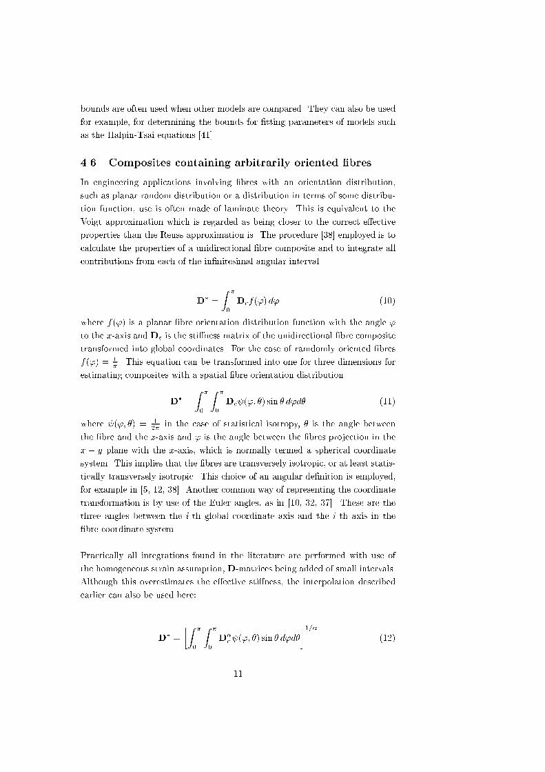
4.6 Composites containing arbitrarily oriented �bres

In engineering applications involving �bres with an orientation distribution,

such as planar random distribution or a distribution in terms of some distribu-

tion function, use is often made of laminate theory. This is equivalent to the

Voigt approximation which is regarded as being closer to the correct e�ective

properties than the Reuss approximation is. The procedure [38] employed is to

calculate the properties of a unidirectional �bre composite and to integrate all

contributions from each of the in�nitesimal angular interval

D� =

Z �

0

Dcf(') d' (10)

where f(') is a planar �bre orientation distribution function with the angle '

to the x-axis and Dc is the sti�ness matrix of the unidirectional �bre composite

transformed into global coordinates. For the case of ramdomly oriented �bres

f(') = 1� . This equation can be transformed into one for three dimensions for

estimating composites with a spatial �bre orientation distribution

D� =

Z �

0

Z �

0

Dc ('; �) sin � d'd� (11)

where ('; �) = 12� in the case of statistical isotropy, � is the angle between

the �bre and the z-axis and ' is the angle between the �bres projection in the

x � y plane with the x-axis, which is normally termed a spherical coordinate

system. This implies that the �bres are transversely isotropic, or at least statis-

tically transversely isotropic. This choice of an angular de�nition is employed,

for example in [5, 12, 38]. Another common way of representing the coordinate

transformation is by use of the Euler angles, as in [10, 32, 37]. These are the

three angles between the i-th global coordinate axis and the i-th axis in the

�bre coordinate system.

Practically all integrations found in the literature are performed with use of

the homogeneous strain assumption, D-matrices being added of small intervals.

Although this overestimates the e�ective sti�ness, the interpolation described

earlier can also be used here:

D� =

�Z �

0

Z �

0

D�c ('; �) sin � d'd�

�1=�(12)

11

where �1 � � � 1 as stated previously.

A simple and quick way of calculating the isotropic sti�ness and the isotropic

shear rigidity of a planar random composite by use of laminate theory [39] is

through employing the approximation

E� =3

8E11 +

5

8E22

G� =1

8E11 +

1

4E22 (13)

where E11 is the sti�ness of the unidirectional lamina in the �bre direction and

E22 is the sti�ness of them in the transverse direction (E11 must be greater than

E22). The greater the di�erence between the moduli is, the more accurate the

expression becomes.

For �brous materials such as paper, Cox's classic model [8] is sometimes em-

ployed. It assumes only the longitudinal sti�ness, Ef , of the �bres and a state of

homogeneous strain. For an isotropic �bre distribution, Young's modulus and

Poisson's ratio become

E� =1

3VfEf

�� =1

3(14)

where Vf is the volume density of the �bre material. This model is not recom-

mended for estimating the properties of multiphase materials, however, since it

neglects the in uence of the transverse sti�ness and the shear sti�ness of the

�bres.

5 Models of Hygroexpansions

An equation for the e�ective hygroexpansion coe�cients of a general 2-phase

material or for the thermal expansion coe�cients, since from a mathematical

point of view the problem envolved is identical, was derived by Levin [27]. It was

extended by Rosen and Hashin [36] to generally anisotropic 2-phase composites

and to an arbitrary phase geometry in the form

�� = �(1) + (�(2)� �(1))(C(2) �C(1))�1(C� �C(1)) (15)

where �� and C� are the e�ective hygroexpansion coe�cients and the e�ective

compliance tensor, respectively. �(i) and C(i), in turn, are the hygroexpansion

12

coe�cients and the compliance tensors of the phases, respectively. For statisti-

cally isotropic composites with isotropic phases, the equation simpli�es to

�� = �(1) +�(2) � �(1)

1=K2 � 1=K1(1=K� � 1=K1) (16)

where K� is the e�ective bulk modulus and K1 and K2 are the phase bulk

moduli. In the case of a transversely isotropic �bre composite with isotropic

�bre and matrix phases, the hygroexpansion components become

��L = �(1) +�(2) � �(1)

1=K2 � 1=K1

�3(1� 2��L)

E�L�

1

K1

�

��T = �(1) +�(2) � �(1)

1=K2 � 1=K1

�3

2k��

3(1� 2��L)

E�L�

1

K1

�(17)

where k� is the e�ective transverse bulk modulus. In [36] a corresponding equa-

tion for the general multiphase e�ective hygroexpansion is also given.

An interesting conclusion to be drawn from equation (15) is that the hygroex-

pansion components follow from the e�ective sti�nesses without further approx-

imations being required. The bounds for the hygroexpansion coe�cients can be

obtained by calculating the bounds for sti�nesses and then calculating the cor-

responding hygroexpansion.

For a composite like that represented in the HPL equation (15), however, is only

applicable at the �rst step in the homogenisation of a single �bre in a matrix

material inclusion, rather than for an entire �bre network. For a network made

up of �bres contained in inclusions, the hygroexpansion can be calculated in

accordance with the homogeneous strain assumption

"� =

Z �

0

Z �

0

D��1D "o ('; �) sin � d'd� (18)

where D is the sti�ness matrix of a homogenised unidirectional �ber composite

at an angle that is transformed into that of the global coordinate system, and

"o is the free hygroexpansion of the same composite.

6 Sti�ness calculation of a HPL

The following illustrates calculation of the sti�ness of a core layer (phenolic resin

impregnated paper) of a high-pressure laminate. The sti�ness properties of the

constituents are taken from [35] which concerns the properties of a single wood

�bre, and from [4], which deals with the sti�ness properties of a phenolic resin.

13

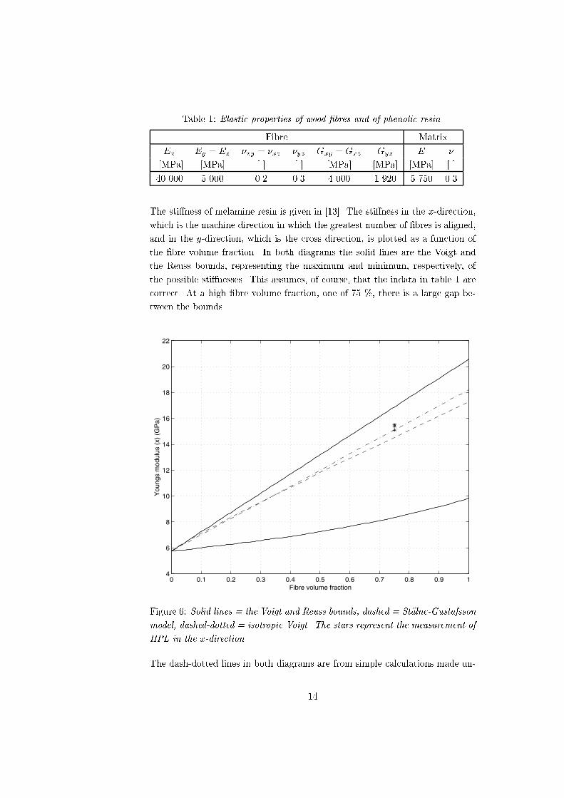
Table 1: Elastic properties of wood �bres and of phenolic resin.

Fibre Matrix

Ex Ey = Ez �xy = �xz �yz Gxy = Gxz Gyz E �

[MPa] [MPa] [-] [-] [MPa] [MPa] [MPa] [-]

40 000 5 000 0.2 0.3 4 000 1 920 5 750 0.3

The sti�ness of melamine resin is given in [13]. The sti�ness in the x-direction,

which is the machine direction in which the greatest number of �bres is aligned,

and in the y-direction, which is the cross direction, is plotted as a function of

the �bre volume fraction. In both diagrams the solid lines are the Voigt and

the Reuss bounds, representing the maximum and minimum, respectively, of

the possible sti�nesses. This assumes, of course, that the indata in table 1 are

correct. At a high �bre volume fraction, one of 75 %, there is a large gap be-

tween the bounds.

0 0.1 0.2 0.3 0.4 0.5 0.6 0.7 0.8 0.9 14

6

8

10

12

14

16

18

20

22

Fibre volume fraction

You

ngs

mod

ulus

(x)

(G

Pa)

Figure 6: Solid lines = the Voigt and Reuss bounds, dashed = St�alne-Gustafsson

model, dashed-dotted = isotropic Voigt. The stars represent the measurement of

HPL in the x-direction.

The dash-dotted lines in both diagrams are from simple calculations made un-

14

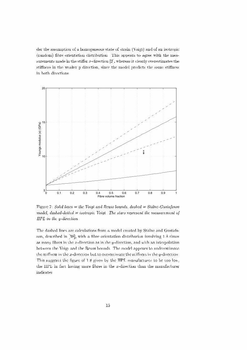
der the assumption of a homogeneous state of strain (Voigt) and of an isotropic

(random) �bre orientation distribution. This appears to agree with the mea-

surements made in the sti�er x-direction [2], whereas it clearly overestimates the

sti�ness in the weaker y-direction, since the model predicts the same sti�ness

in both directions.

0 0.1 0.2 0.3 0.4 0.5 0.6 0.7 0.8 0.9 15

10

15

20

Fibre volume fraction

You

ngs

mod

ulus

(x)

(G

Pa)

Figure 7: Solid lines = the Voigt and Reuss bounds, dashed = St�alne-Gustafsson

model, dashed-dotted = isotropic Voigt. The stars represent the measurement of

HPL in the y-direction.

The dashed lines are calculations from a model created by St�alne and Gustafs-

son, described in [38], with a �bre orientation distribution involving 1.8 times

as many �bres in the x-direction as in the y-direction, and with an interpolation

between the Voigt and the Reuss bounds. The model appears to underestimate

the sti�ness in the x-direction but to overestimate the sti�ness in the y-direction.

This suggests the �gure of 1.8 given by the HPL manufacturer to be too low,

the HPL in fact having more �bres in the x-direction than the manufacturer

indicates.

15

References

[1] Aboudi, J. (1991). Mechanics of Composite Materials, Elsevier, Amster-

dam, The Netherlands, 14-18.

[2] Andersson, B. (1999). Composite materials' hygro-mechanical properties,

Masters thesis, Report TVSM-3018, Div. of Structural Mechanics, Lund

University, Sweden.

[3] Adl Zarrabi, B. (1998). Hygro-Elastic Deformation of High Pressure Lam-

inates, Doctoral thesis, Div. of Building Material, Chalmers University of

Technology, G�oteborg, Sweden

[4] Barth, Th. (1984). "Der Ein uss der Feuchteaufnahme auf die mechanis-

chen Eigenschaften von Phenolplasten." Z. Werksto�tech, Verlag Chemie,

Weinheim, Germany, 15, 299-308.

[5] Camacho, C.W., Tucker, C.L. (1990). "Sti�ness and Thermal Expansion

Predictions for Hybrid Short Fiber Composites". Polymer Composites, 11,

229-239.

[6] Carman, G.P., Reifsnider, K.L. (1992). "Micromechanics of Short-Fiber

Composites", Composites Science and Technology, 43, 137-146.

[7] Chen, H.-J., Tsai, S.W. (1996). "Three-Dimensional E�ective Moduli of

Symmetric Laminates". Journal of Composite Materials, 30, 906-917.

[8] Cox, H.L. (1951). "The elasticity and strength of paper and other �brous

materials." Brittish Journal of Applied Physics, 3, 72-79.

[9] Dinwoodie, J.M. (1989).Wood: nature's cellular, polymeric �bre-composite,

The Institute of Metals, London, 57. Dinwoodie { Wood: nature's cellular,

polymeric �bre-composite : Trsi�ror

[10] Dunn, M. L., Ledbetter, H., Heyliger, P. R. and Choi, C. S. (1996). "Elas-

tic constants of textured short-�ber composites." J. Mech. Phys. Solids,

Elsevier, Amsterdam, The Netherlands, 44, 1509-1541.

[11] Eshelby, J.D, (1957). "The determination of the �eld of an elliptical inclu-

sion and related problems", Proceedings of the Royal Society, London, Vol

A, No. 241, p 376-396.

[12] Fu, S.-Y. Lauke, B. (1998). "An analytical characterization of the

anisotropy of the elastic modulus of misaligned short-�ber-reinforced poly-

mers." Composites Science and Technology, 58, 1961-1972.

16

[13] Hagstrand, P.-O.Mechanical Analysis of Melamine-Formaldehyde Compos-

ites, Doctoral thesis, Dept. of Polymeric Material, Chalmers University of

Technology, G�oteborg, Sweden.

[14] Halpin, J.C., Kardos, J.L. (1976). "The Halpin-Tsai equations: A review."

Polymer Engineering and Science, 16, 344-352.

[15] Hashin, Z. (1983) "Analysis of Composite Materials, A Survey", Journal

of Applied Mechanics, 9, 481-505.

[16] Hashin, Z. (1979) "Analysis of Properties of Fiber Composites with

Anisotropic Constituents" Journal of Applied Mechanics, 46, 543-550.

[17] Hashin, Z., Shtrikman, S. (1963). "A variational approach to the theory of

the elastic behaviour of multiphased materials." J. Mech. Phys. Solids, 11,

127-140.

[18] Hashin, Z. (1965). "On Elastic Behaviour of Fibre Reinforced Materials

of Arbitrary Transverse Phase Geometry". Journal of the Mechanics and

Physics of Solids, 13, 119-134.

[19] Hashin, Z., Rosen, B.W. (1964). "The Elastic Moduli of Fiber-Reinforced

Materials". Journal of Applied Mechanics, 6, 223-232.

[20] Heyden, S. (2000). Network modelling for the evaluation of mechanical

properties of cellulose �bre u�., Doctoral thesis, Report TVSM-1011, Div.

of Structural Mechanics, Lund University, Sweden.

[21] Hill, R. (1963) "Elastic Properties of Reinforced Solids: Some Theoretical

Principals". Journal of the Mechanics and Physics of Solids, 11, 357-372.

[22] Hill, R. (1952) "Elastic Behaviour of a Crystalline Aggregate". Proceedings

of the Physical Society, Section A, 349-354.

[23] Hill, R. (1965) "A Self Consistent Mechanics of Composite Materials".

Journal of the Mechanics and Physics of Solids, 13, 213-222.

[24] Hillerborg, A. (1986). Kompendium i Byggnadsmateriall�ara FK, Division

of Building Materials, Lund University, Sweden.

[25] Hult, J., Bjarnehed, H. (1993). Styvhet och Styrka - Grundl�aggande Kom-

positmekanik, Studentlitteratur, Lund, Sweden.

[26] Ju, J.W., Zhang, X.D. (1998). "Micromechanics and E�ective Transverse

Elastic Moduli of Composites with Randomly Located Aligned Circular

Fibers". International Journal of Solids and Structures, 35, 941-960.

17

[27] Levin, V.M. (1967). "On the Coe�cients of Thermal Expansion of Hetero-

geous Materials". Mechanics of Solids, 2, 58-61.

[28] Luciano, R., Barbero, E.J. (1994). "Formulas for the Sti�ness of Com-

posites with Periodic Microstructure". International Journal of Solids and

Structures, 31, 2933-2944.

[29] Lukkassen, D., Persson, L.-E., Wall, P. (1994). Some Engineering and

Mathematical Aspects on the Homogenization Method for Computing Ef-

fective Moduli and Microstresses in Elastic Composite Materials, Research

Report 2, Dept. of Mathematics, Lule�a University of Technology, Sweden.

[30] Moavenzadeh, F. (1990). Concise Encyclopedia of Building and Construc-

tion Materials, New York, USA.

[31] Mori, T., Tanaka, K. (1973) "Average Stress in Matrix and Average Elastic

Energy of Materials with Mis�tting Inclusions". Acta Metallurgica, 21, 571-

574.

[32] Munson-McGee, S.H., McCullough, R.L. (1994). "Orientation Parameters

for the Speci�cation of E�ective Properties of Heterogeneous Materials".

Polymer Engineering and Science, 34, 361-370.

[33] Oksman, K. (1997). Improved Properties of Thermoplastic Wood Flour

Coumposites, Doctoral thesis, 1997-17, Div. of Wood Technology, Lule�a

University of Technology, Sweden.

[34] Persson, L.E., Persson, L., Svanstedt, N., Wyller, J. (1993) The Homoge-

nization Method, Studentlitteratur, Lund, Sweden.

[35] Persson, K. (1997). Modelling of wood properties by a micromechanical ap-

proach., Licentiate thesis, Report TVSM-3018, Div. of Structural Mechan-

ics, Lund University, Sweden.

[36] Rosen, B.W., Hashin, Z. (1970) "E�ective Thermal Expansion Coe�cients

and Speci�c Heats of Composite Materials", Inernational Journal of Engi-

neering Science, 8, 157-173.

[37] Sayers, C.M. (1992). "Elastic anisotropy of short-�bre reinforced compos-

ites." International Journal of Solids and Structures, 29, 2933-2944.

[38] St�alne, K., Gustafsson, P.J. (2000). "A 3D Model for Analysis of Sti�ness

and Hygroexpansion Properties of Fibre Composite Materials", Journal of

Engineering Mechanics, in press.

[39] Tsai, S.W., Pagano, N.J. (1968). "Invariant Properties of Composite Mate-

rials" Composite Materials Workshop, Technomic Publishing Co. Stamford,

Connecticut, 233-253.

18

[40] Tucker, C.L., Liang, E. (1999). "Sti�ness Predictions for Unidirectional

Short-Fiber Composites: Review and Evaluation" Composites Science and

Technology 59, 655-671.

[41] Wall, P. (1994). A Comparison of Homogenization, Hashin-Shtrikman

Bounds and the Halpin-Tsai Equations, Research Report 21, Dept. of Math-

ematics, Lule�a University of Technology, Sweden.

19

II

Analysis of Fibre Composite Models

for Sti�ness and Hygroexpansion

Kristian St�alne

Division of Structural Mechanics

Lund University, Sweden

Abstract

In this report analytical models for elastic properties and hygroexpansion of

�bre composite materials are presented. The cases of homogeneous strain and

homogeneous stress are studied for 2D and 3D states of stress. There is also

an interpolation between the two cases and it is shown that the interpolation

is unambiguous and ful�lls the coordinate invariance principle.

Keywords

Micromechanical model, mechanical properties, composite material, sti�ness,

hygro expansion.

F�orord

This is the �rst report produced in the research project "Composite Material

Moisture Mechanics" �nanced by the research collegue " Wood Mechanics".

I would like to thank my supervisor Per Johan Gustafsson for help and en-

couragement.

Kristian St�alne

Lund, September 1999

Sammanfattning

I rapporten presenteras analytiska modeller f�or styvhet och hygroexpansion

f�or �berkompositmaterial. Modellerna utg�ar fr�an fallen homogent t�ojningstillst�and

respektive homogent sp�anningstillst�and och kan till�ampas i b�ade tv�a och tre

dimensioner. Vidare f�oresl�as en interpolation mellan de b�ada extremfallen

och det visas att denna �ar entydig och koordinatinvariant.

Inneh�all

1 Introduction 1

2 Transformation of stresses and strains 3

3 The sti�ness matrix at homogeneous states 6

3.1 Fibre network at homogeneous state of strain . . . . . . . . . 6

3.2 Fibre network at homogeneous state of stress . . . . . . . . . . 7

3.3 Sti�ness matrices of composite materials with two phases . . . 9

4 Hygroexpansion 10

4.1 Serial coupling . . . . . . . . . . . . . . . . . . . . . . . . . . . 10

4.2 Parallel coupling . . . . . . . . . . . . . . . . . . . . . . . . . 11

5 An interpolation model 13

5.1 Calculation of D� . . . . . . . . . . . . . . . . . . . . . . . . . 14

5.2 Problem . . . . . . . . . . . . . . . . . . . . . . . . . . . . . . 15

5.3 Rede�nition of stress and strain vectors . . . . . . . . . . . . . 17

5.4 Some matrix theory . . . . . . . . . . . . . . . . . . . . . . . . 18

6 Generalisation to three dimensions 21

6.1 Coordinate transformation . . . . . . . . . . . . . . . . . . . . 22

6.2 Orientation distribution function . . . . . . . . . . . . . . . . 25

6.3 Integration of all �bres . . . . . . . . . . . . . . . . . . . . . . 27

7 Concluding remarks 28

7.1 Future work . . . . . . . . . . . . . . . . . . . . . . . . . . . . 29

4

1 Introduction

The usage of �bre composite materials is today increasing in di�erent ap-

plications in order to combine sti�ness and strength with low weight. This

leads to a greater need of models for prediction of the properties and be-

haviour of the composite material from the constituents properties. There

are many di�erent homogenisations and network mechanics models in use

today [1, 2, 3]. The most dominating in this case is probably the Halpin-Tsai

equations [4] which has been used frequently since the 60s , mostly for short

�bre composites.

The models discussed here shows di�erent alternatives when computing the

sti�ness matrix and hygroexpansion of a composite material. Indata to the

calculation of sti�ness is the sti�ness matrices of the constituting material

componetns, volume fractions and orientation distribution of the �bres. The

hygroexpansion of the composite is estimated in a similair way from the con-

stituents free hygroexpansions. The results contains bounds for sti�ness and

hygroexpansion and an interpolation between the extreme cases according to

a generalisation using the method of weighted potence means.

1

This report contains coordinate transformations for stresses, strains and sti�-

ness matrices, followed by a summation of sti�ness matrices and an integra-

tion over all �bres. Then the hygroexpansion is taken into account after which

the interpolation model is presented for the case of plane stress. Using matrix

theory and an alternative de�nition of the stress and strain vectors the model

is shown to be coordinate invariant. Finally the model is generalised to three

dimensions.

2

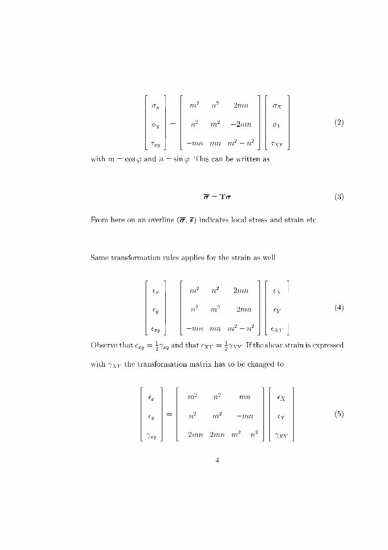
2 Transformation of stresses and strains

When a coordinate system is rotated the angle ' are the stresses transformed

at the state of plane stress according to [5]

�x = �X cos2 '+ �Y sin2 '+ 2�XY sin' cos'

�y = �X sin2 ' + �Y cos2 '� 2�XY sin' cos' (1)

�x = ��X sin' cos'+ �Y sin' cos'+ �XY (cos2 '� sin2 ')

where x-y are local coordinates and X-Y are global coordinates.

x

y

Y

X

ϕ

Figur 1: Rotation of the coordinate system with the angle ' from the global

(X-Y ) to the �bres coordinate system x-y.

This can be written in matrix notation as

3

2666666664

�x

�y

�xy

3777777775=

2666666664

m2 n2 2mn

n2 m2 �2mn

�mn mn m2 � n2

3777777775

2666666664

�X

�Y

�XY

3777777775

(2)

with m = cos' and n = sin'. This can be written as

� = T� (3)

From here on an overline (�, �) indicates local stress and strain etc.

Same transformation rules applies for the strain as well

2666666664

�x

�y

�xy

3777777775=

2666666664

m2 n2 2mn

n2 m2 �2mn

�mn mn m2 � n2

3777777775

2666666664

�X

�Y

�XY

3777777775

(4)

Observe that �xy =1

2 xy and that �XY = 1

2 XY . If the shear strain is expressed

with XY the transformation matrix has to be changed to

2666666664

�x

�y

xy

3777777775=

2666666664

m2 n2 mn

n2 m2 �mn

�2mn 2mn m2 � n2

3777777775

2666666664

�X

�Y

XY

3777777775

(5)

4

or in short notation

� = T�T� (6)

where T�T is the inverse of the transpose of T. The di�erence between trans-

formation of stress and strain can be eliminated by using �xy instead of xy

and compensate for in the sti�ness matrix by doubling element Q44. From

now on � =

"�X �Y XY

#T. Observe that

TT 6= T�1 (7)

5

3 The sti�ness matrix at homogeneous states

3.1 Fibre network at homogeneous state of strain

The �bres are considered as orthotropic discs with di�erent orientaion. At

homogeneous state of strain it is assumed that alla �bres have the same strain

at all points. This is equivalent to laminate theory. The sti�ness matrix, D,

can be calculated by summing of the transformation of each �bre sti�ness

matrix of each orientation. The consitutive equation � = D� for the �bre in

the local coordinate system written with all components is

� =1

1� �xy�yx

2666666664

Ex �yxEx 0

�xyEy Ey 0

0 0 (1� �xy�yx)Gxy

3777777775� (8)

This gives, with the transformation equation for stress and strain,

� = T�1� = T�1D� = T�1DT�T� (9)

and the sti�ness matrix can in the global coordinates be written as

6

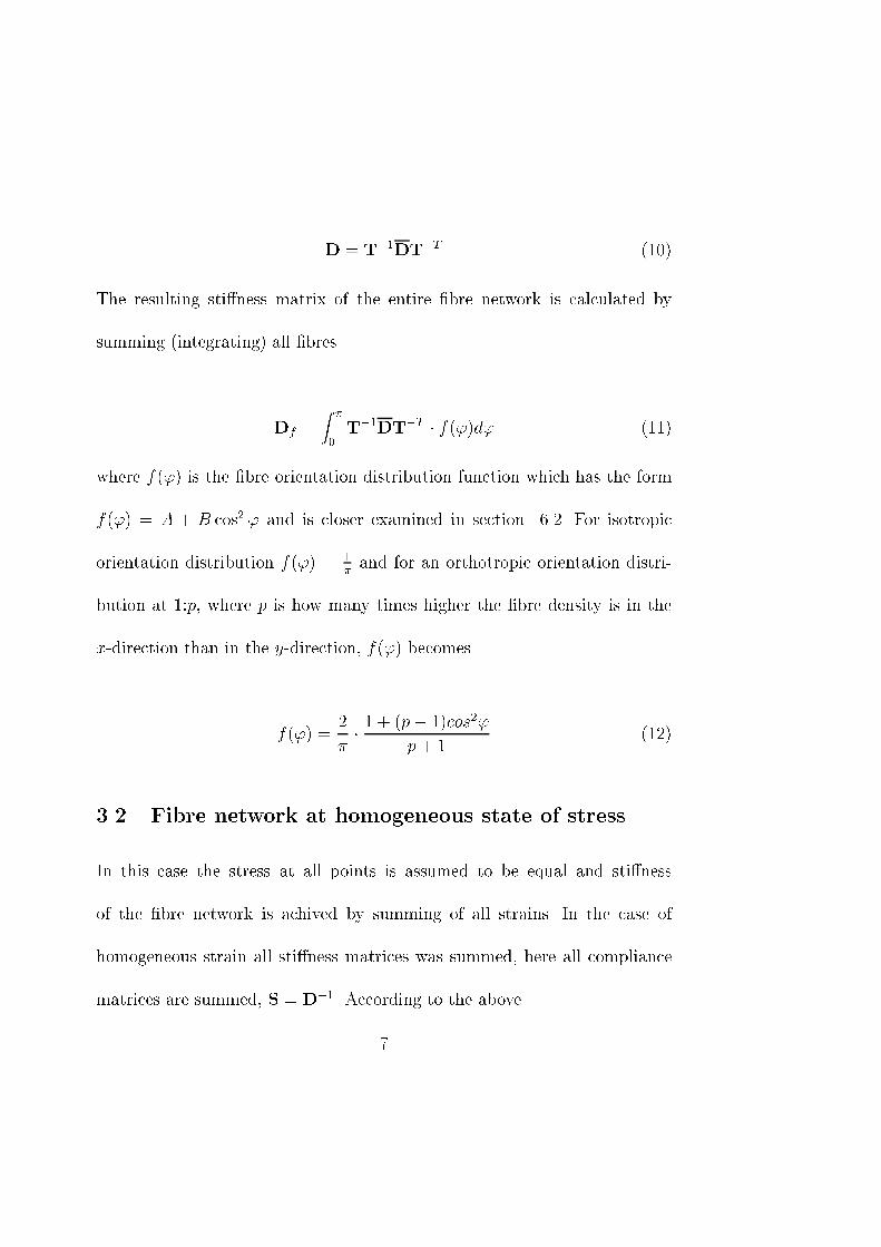
D = T�1DT�T (10)

The resulting sti�ness matrix of the entire �bre network is calculated by

summing (integrating) all �bres.

Df =Z �

0

T�1DT�T � f(')d' (11)

where f(') is the �bre orientation distribution function which has the form

f(') = A + B cos2 ' and is closer examined in section 6.2. For isotropic

orientation distribution f(') = 1

�and for an orthotropic orientation distri-

bution at 1:p, where p is how many times higher the �bre density is in the

x-direction than in the y-direction, f(') becomes

f(') =2

�� 1 + (p� 1)cos2'

p+ 1(12)

3.2 Fibre network at homogeneous state of stress

In this case the stress at all points is assumed to be equal and sti�ness

of the �bre network is achived by summing of all strains. In the case of

homogeneous strain all sti�ness matrices was summed, here all compliance

matrices are summed, S = D�1. According to the above

7

−2 −1.5 −1 −0.5 0 0.5 1 1.5 20

0.05

0.1

0.15

0.2

0.25

0.3

0.35

0.4

0.45

0.5

Vinkel (rad)

För

deln

ings

funk

tion

a

b

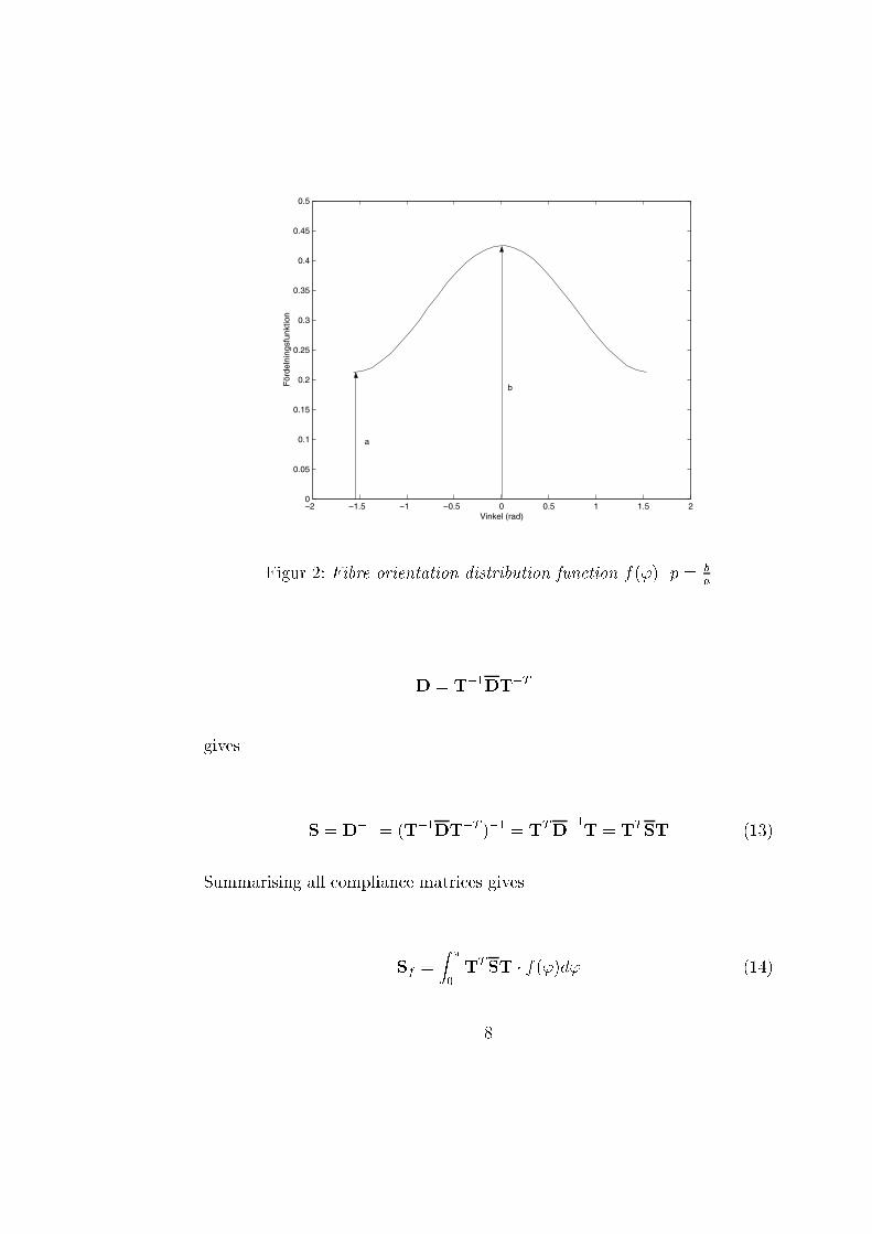
Figur 2: Fibre orientation distribution function f('). p = ba

D = T�1DT�T

gives

S = D�1 = (T�1DT�T )�1 = TTD�1

T = TTST (13)

Summarising all compliance matrices gives

Sf =Z �

0

TTST � f(')d' (14)

8

or

Df =�Z �

0

TTD�1

T � f(')d'��1

=�Z �

0

(T�1DT�T )�1 � f(')d'��1

(15)

3.3 Sti�ness matrices of composite materials with two

phases

If another material is added to the �bre network, the components sti�ness

matrices can be summarised, weighted with the volume fractions respectively,

in analogy with the integration

Dc = VmDm + VfDf (16)

according to the model of parallel coupling. That can also be done using the

serial coupling model

Dc =�VmD

�1

m + VfD�1

f

��1

(17)

9

4 Hygroexpansion

The free hygroexpansion of a �bre is denoted �0 in the local coordinate system

of the �bre and is de�ned

�0 =

2666666664

�L

�T

0

3777777775= p(�)

2666666664

�L(max)

�T (max)

0

3777777775

(18)

where p(�) is the relative strain as a function of the relative humidity, �,

�L(max) and �T (max) are the hygroexpansion at saturated humidity [7].

4.1 Serial coupling

The simplest way of calculating the hygroexpansion of a composite material

is the serial coupling model. The total strain is the sum of the strains of all

components multiplied with the respective volume fractions

�0

c = V1�0

1+ V2�

0

2(19)

where �01and �0

2are the components free hygroexpansion strains. For k num-

ber of components the total strain is

10

� =kXi=1

Vi�0

i (20)

The corresponding integral for all �bre directions the total strain �0

f of the

�bre network becomes

�0

f =Z �

0

�0 � f(')d' =

Z �

0

TT�0 � f(')d' (21)

4.2 Parallel coupling

Parallel coupling means a homogeneous state of strain, which at a constrained

hygroexpansion leads to the stress

� = V1�1 + V2�2 (22)

where �1 = D1�0

1and �2 = D2�

0

2. This stress gives the free hygroexpansion

strain

�0

c = D�1

c � = V1D�1

c D1�0

1+ V2D

�1

c D2�0

2(23)

where �01and �

0

2are the constituents free hygroexpansion strains. A general

expression for k number of material is

11

�0 =

kXi=1

ViD�1

c Di�0

i (24)

and the integration for all �bres in a network is

�0

f = D�1

c

Z �

0

� � f(')d' =Z �

0

D�1

c T�1D�0 � f(')d' (25)

or

�0

f =Z �

0

D�1

c DTT�0 � f(')d' (26)

12

5 An interpolation model

The idea of this model is to make a mathematical interpolation between the

cases of parallel and serial coupling. One way to achieve this is by inserting

a potence, "�" over all matrices. The parameter � works as a �tting param-

eter and can be �tted to measurements but also estimated regarding to the

geometry of the composite.

D�c = VmD

�m + VfD

�f (27)

here � = 1 corresponds to the parallel coupling case and � = �1 corresponds

to the serial coupling case. The idea comes from the compendium in building

materials [7] where it is described in one dimension, i.e. for scalar properties:

E�c = VmE

�m + VfE

�f (28)

which for n! 0 appproaches

Ec = EVmm E

Vff (29)

which is the geometrical mean of Em och Ef .

13

According to Wall [8] even the Halpion-Tsai equations can be seen as an

interpolation between arithmetic mean, � = 1, and harmonic mean, � =

�1. He also mensions the weighted potence mean, equation (28), for scalar

properties.

5.1 Calculation of D�

The potence, �, inserted is an operation carried out on the entire matrix,

and not elementwise. Like other matrix functions this operation is done by

diagonalising the matrix and performing the operation on the diagonal ele-

ments

D� = (Q�Q�1)� = Q(�)�Q�1 = Q

2666666664

��1

0 0

0 ��2

0

0 0 ��3

3777777775Q�1 (30)

The requirement for this to be possible is that D is diagonalisable and posi-

tively di�nite, which easily can be shown if D is linear elastic.

14

5.2 Problem

Now the corresponding procedure for hygroexpansion is analysed. For a com-

posite with two constituents the equations (19) and (23) are combined to

�0 = V1(D

�1

c D1)�+12 �

0

1+ V2(D

�1

c D2)�+12 �

0

2(31)

Still � = 1 corresponds to parallel coupling and � = �1 to serial coupling.

One small problem is that the strain �0

c not equals the free strains of the

constituents when they are set to be equal �01= �

0

2for all �. �0c is only equal

to �01and �

0

2when � = 1 or � = �1.

It is desirable to perform the calculation of the sti�ness matrix and the

hygroexpansion strain for a �bre network for all � even for the integration

of the �bre orienation directions.

Df =�Z �

0

(T�1DT�T )� � f(')d'�1=�

(32)

and for hygroexpansion

�0

f =Z �

0

(D�1

c D)�+12 TT

�0 � f(')d' (33)

15

The big problem is that this calculation of Df is depending on the coordi-

nate system used. When equation (27) is solved it is natural to chose the

coordinate system in the �bres direction of orthotropy (MD), but now the

�bres will be weighted di�erently depending on the alignment. Regardless of

this fact it is unacceptable for a fysical law to be dependent on the chosen

coordinate system. One example is

D�c = VmD

�m + VfD

�f

which for another arbitrary chosen coordinate system can be written as

(T�1DcT�T )� = Vm(T

�1DmT�T )� + Vf(T

�1DfT�T )�

In order to make this coordinate invariant there have to be a way of getting

rid of all T. For example

(T�1)�D�c (T

�T )� = Vm(T�1)�D

�f (T

�T )� + Vf(T�1)�D

�m(T

�T )� (34)

Unfortunatly this simpli�cation, or any other, is not possible since

A�B� 6= (AB)� (35)

16

thus the coordinate invariance not can be shown.

5.3 Rede�nition of stress and strain vectors

The solution of the problem of coordinate invariance is de�ning the stress

and strain vectors as

� =

2666666664

�x

�y

p2 �xy

3777777775; � =

2666666664

�x

�y

p2 �xy

3777777775

(36)

This is not new, it is mentioned in The Mechanics of Constitutive Modelling

[10] brie y together with a few references. With this de�nition the stress and

strain vectors are transformed using the same transformation matrix,

� = T�; � = T�; (37)

The, now orthogonal, transformation matrix is de�ned as

T =

2666666664

m2 n2p2mn

n2 m2 �p2mn

�p2mn p2mn m2 � n2

3777777775

(38)

17

5.4 Some matrix theory

The reason of de�ning the shear strain and shear stress components with

the factorp2 instead of as in equation(2), (4) and (5) is that the sti�ness

matrix, D, now is independent of in which coordinate system it is calculat-

ed. The new choice of strain and sti�ness de�nitions gives the two necessary

properties:

1) The sti�ness matrix is symmetric and positively de�nite. This can be

shown by using thermodynamics which states that the strain energy, W ,

allways is positive when the strains are not equal to zero. This can be written

W =1

2�TD� < 0 (39)

which is equivalent to D being positively de�nite. In that case the spectre of

the matrix is positive, i.e. all eigenvalues of D are positive if the matrix is

symmetric. This means that there are no unpleasant involvements of complex

numbers which arises when a negative base is raised to non-integer potence.

2) The transformation of the strains are carried out in the same way as for

the stresses. This is decisive when the coordinate invariance is shown. The

18

constitutive relation is now:

� = D� =1

1� �xy�yx

2666666664

Ex �xEy 0

�xEy Ey 0

0 0 (1� �xy�yx) � 2Gxy

3777777775� (40)

The sti�ness matrix is transformed as

� = T�1� = T�1D� = T�1DT�

)

D = T�1DT (41)

When the engineering strains (5) are used only condition 1) is ful�lled and

when the tensor components (4) are used only condition 2) is ful�lled. With

the new de�nition both conditions are ful�lled.

When the coordinate invariance of the sti�ness matrix is to be shown, the

following equation is used [11]

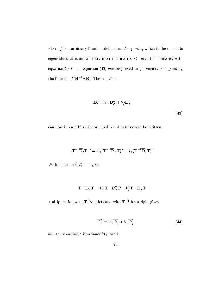
f(B�1AB) = B�1f(A)B (42)

19

where f is a arbitrary function de�ned on As specter, which is the set of As

eigenvalues. B is an arbitrary inversible matrix. Observe the similarity with

equation (30). The equation (42) can be proved by potence serie expanding

the function f(B�1AB). The equation

D�c = VmD

�m + VfD

�f

(43)

can now in an arbitrarily oriented coordinate system be written

(T�1DcT)� = Vm(T

�1DmT)� + Vf(T

�1DfT)�

With equation (42) this gives

T�1D�

cT = VmT�1D

�

cT+ VfT�1D

�

fT

Multiplication with T from left and with T�1 from right gives

D�c = VmD

�c + VfD

�f (44)

and the coordinate invariance is proved.

20

6 Generalisation to three dimensions

In the three dimensional case the �bre orientation is described as a projec-

tion on a unit semisphere with the radius 1. The spherical coordinates on the

semisphere represent the two angles, ' and �, where � is the angle between

the positive z-axis (0 � � � �) and the �bre and ' is the angle between the

�bres projection at the X-Y plane and the X-axis in the positive direction

(0 � ' � �). The angles are shown in �gure 3.

ϕ

θ

Y

x

y

X

Zz

Figur 3: Coordinate transformation in three dimensions.

21

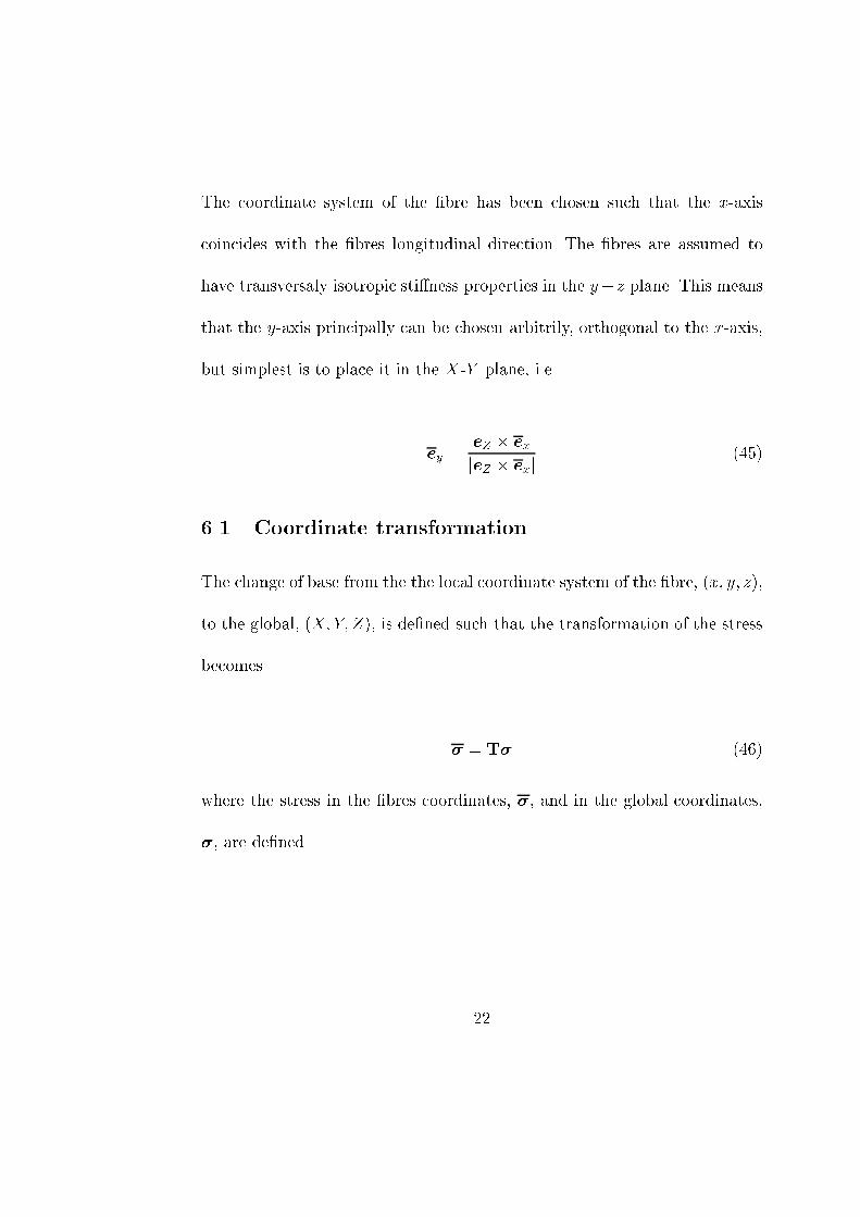
The coordinate system of the �bre has been chosen such that the x-axis

coincides with the �bres longitudinal direction. The �bres are assumed to

have transversaly isotropic sti�ness properties in the y�z plane. This means

that the y-axis principally can be chosen arbitrily, orthogonal to the x-axis,

but simplest is to place it in the X-Y plane, i.e.

ey =eZ � ex

jeZ � exj (45)

6.1 Coordinate transformation

The change of base from the the local coordinate system of the �bre, (x; y; z),

to the global, (X; Y; Z), is de�ned such that the transformation of the stress

becomes

� = T� (46)

where the stress in the �bres coordinates, �, and in the global coordinates,

�, are de�ned

22

� =

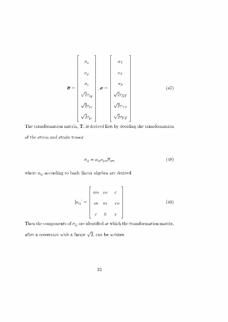
2666666666666666666666664

�x

�y

�z

p2�xy

p2�xz

p2�yz

3777777777777777777777775

;� =

2666666666666666666666664

�X

�Y

�Z

p2�XY

p2�XZ

p2�Y Z

3777777777777777777777775

(47)

The transformation matrix, T, is derived �rst by deciding the transformation

of the stress and strain tensor

�ij = aiqajm�qm (48)

where aij according to basic linear algebra are derived

[aij] =

2666666664

sm sn c

sn m �cn

c 0 s

3777777775

(49)

Then the components of �ij are identi�ed at which the transformation matrix,

after a correction with a factorp2, can be written

23

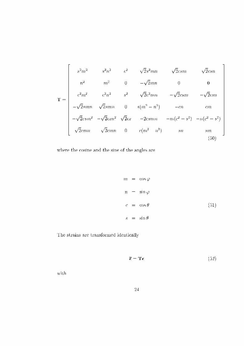
T =

2666666666666666666666664

s2m2 s2n2 c2p2s2mn

p2csm

p2csn

n2 m2 0 �p2mn 0 0

c2m2 c2n2 s2p2c2mn �p2csm �p2csn

�p2smn p2smn 0 s(m2 � n2) �cn cm

�p2csm2 �p2csn2 p2cs �2csmn �m(c2 � s2) �n(c2 � s2)

p2cmn �p2cmn 0 �c(m2 � n2) �sn sm

3777777777777777777777775

(50)

where the cosine and the sine of the angles are

m = cos'

n = sin'

c = cos � (51)

s = sin �

The strains are transformed identically

� = T� (52)

with

24

� =

2666666666666666666666664

�x

�y

�z

p2�xy

p2�xz

p2�yz

3777777777777777777777775

; � =

2666666666666666666666664

�X

�Y

�Z

p2�XY

p2�XZ

p2�Y Z

3777777777777777777777775

(53)

The transformation of the sti�ness matrix is now like before

D = T�1DT (54)

6.2 Orientation distribution function

The three dimensional distribution function, ('; �), indicates how high the

�bre density is in a certain direction. The number of �bres at the surface

element dS on the unit semisphere is V = ('; �)dS and the share within a

certain interval of angle, '1 � ' � '2 and �1 � � � �2, is

V =Z '2

'1

Z �2

�1('; �)dS =

Z '2

'1

Z �2

�1('; �) sin �d'd� (55)

since dS = r2 sin �d'd� = sin �d'd�. r2 sin � is a scale factor (h' = r sin �

25

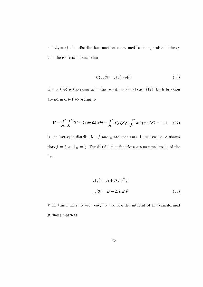
and h� = r). The distribution function is assumed to be separable in the '-

and the � direction such that

('; �) = f(') � g(�) (56)

where f(') is the same as in the two dimensional case (12). Both function

are normalised according to

V =Z �

0

Z �

0

('; �) sin �d'd� =Z �

0

f(')d' �Z �

0

g(�) sin �d� = 1 � 1 (57)

At an isotropic distribution f and g are constants. It can easily be shown

that f = 1

�and g = 1

2. The distribution functions are assumed to be of the

form

f(') = A+B cos2 '

g(�) = D + E sin2 � (58)

With this form it is very easy to evaluate the integral of the transformed

sti�ness matrices.

26

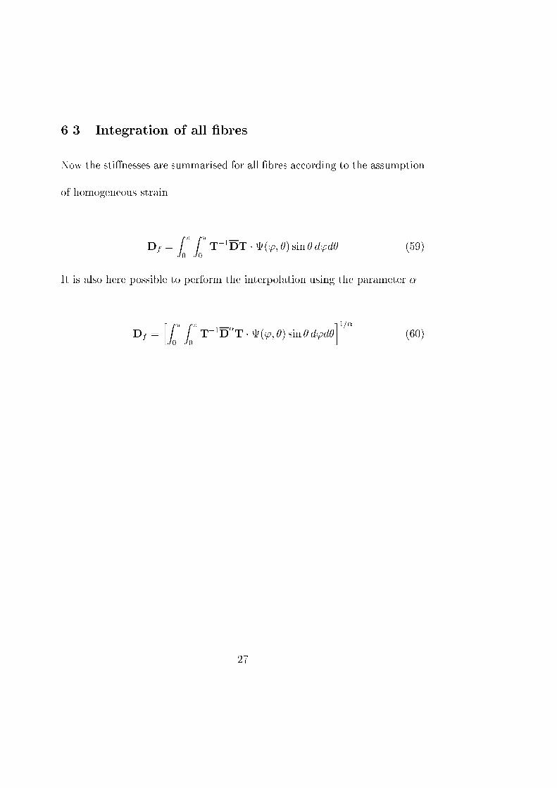
6.3 Integration of all �bres

Now the sti�nesses are summarised for all �bres according to the assumption

of homogeneous strain

Df =Z �

0

Z �

0

T�1DT �('; �) sin � d'd� (59)

It is also here possible to perform the interpolation using the parameter �

Df =�Z �

0

Z �

0

T�1D�T �('; �) sin � d'd�

�1=�(60)

27

7 Concluding remarks

This report describes how the stresses and strains are transformed in the

plane as well as in the space. This have made it possible to summarise the

�bres and the matrix material sti�ness matrices to di�erent kinds of means

for the entire composite under the state och homogeneous strain and homo-

geneous state of stress. This corresponds to the upper and the lower extreme

values for the sti�ness of the composite. Analogous moisture induced strain,

hygroexpansion, have been summarised, which also can be used e.g. at strains

caused by an increase in temperature.

The novelty here is the interpolation between the cases of parallel coupling

and serial coupling according to the method of weighted potence mean is ex-

panded from usage on scalar properties to usage on material sti�ness proper-

ties at two- and three dimensional states of stress. The parameter, �, control-

ling the interpolation can be adapted to �t measurement data or eventually

be estimated according to the geometry of the composite. By a suitable def-

inition of stress and strain vectors the interpolation method has been shown

to be coordinate invariant and computed sti�nesses are thus unambigous.

28

One drawback using the model in its present form is that it does not take

the geometry of the �bres into consideration. One example is if it would be

applied on a glass�bre-epoxy composite where the �bres as well as the matrix

material are isotropic and where all �bres are aligned in one direction. The

longitudinal and transversal sti�ensses di�er often, typically with a factor

3-4, which can not be predicted by this model. One interpretation is that

the material have di�erent � in the di�erent directions. In order to take the

�bre geometries in consideration there might be a possibility of performing

som sort of homogenisation of a single �bre in a small environment of matrix

material.

7.1 Future work

A similair interpolation between serial and parallel coupling for hygroexpan-

sion were studied. One problem here was that the function did not behave

in a, physically speaking, reliable way in all situations. One example is when

both components hygroexpansion properties where set to be equal. Then

the composites hygroexpansion should be equal to the of the comsitituents.

The hygroexpansion was equal to the constituents for the cases of � = 1

and � = �1, but not in between. One alternative, although not as elegant

29

mathematically speaking, is to make a linear interpolation between parallel

coupling and serial coupling

�0

c =1 + �

2�0

p +1� �

2�0

s (61)

where �0p is the composites free hygroexpansion computed under parallel cou-

pling and �0s under serial coupling. Other possibilities can also come into con-

sideration.

One detail worth investigation is what happens at when � ! 0 which cor-

responds to the geometrical mean. It is uncertain if it is as easy as in the

scalar case, equation (29), and if it is unambigous. It may not be of greater

practical importance since it is possible to choose a value of � su�ciently

close to 0. But it is still desirable to show that the theory is de�ned in the

entire interval �1 � � � 1.

30

Referenser

[1] Aboudi, J. Mechanics of Composite Materials, Elsevier, NY (1991)

[2] Hashin, Z. The Elastic Moduli of Fiber-Reinforced Materials, Journal of

Applied Mechanics (1964)

[3] Heyden, S. A Network Model Applied to Cellulose Fibre Materials,

Progress in Paper Physics (1996)

[4] Halpin, JC. Kardos, JC. The Halpin-Tsai equations: A review. Polym.

Eng. Sci. (1976)

[5] Benham, PP. Mechanics of Engineering Materials, Addison, Harlow

(1996)

[6] Heyden, S. How to derive an analytical network mechanics theory, Di-

vision of Structural Mechanics, Lund University (1998)

[7] Hillerborg, A. Kompendium i Byggnadsmateriall�ara FK, Lund (1986)

[8] Wall, P. A Comparison of Homogenisation, Hashin-Shtrikman Bounds

and the Halpin-Tsai Equations, Institutionen f�or Matematik, Lule�a

Tekniska Universitet (1994)

31

[9] Nevander, LE. Fukthandbok. Svensk byggtj�anst, Schmids (1981)

[10] Ottosen, NS. Ristinmaa, M, The Mechanics of Constitutive Modelling,

Division of Solid Mechanics, Lund University (1996)

[11] Spanne, S. F�orel�asningar i matristeori, Department of Mathematics,

Lund University (1994)

32

III

A 3D Model for Analysis of Sti�ness

and Hygroexpansion Properties of

Fibre Composite Materials

Kristian St�alne and Per Johan Gustafsson

Division of Structural Mechanics

Lund University, Sweden

A 3D Model for Analysis of Sti�ness and

Hygroexpansion Properties of Fibre Composite

Materials

Kristian St�alne�, Per-Johan Gustafssony

Keywords: wood, �bre, particle, composite, analytical, modelling, sti�ness, hy-

groexpansion, homogenisation

Abstract

A three dimensional model for sti�ness and hygroexpansion of �bre and

particle composite materials is presented. The model is divided into two

steps, �rst a homogenisation of a single �bre with a coating representing

the matrix material, then a network mechanics modelling of the assem-

bly of coated �bres that constitutes the composite material. The network

modelling is made by a �bre orientation integration including a linear and

an exponential interpolation between the extreme case of homogenous

strain and the extreme case of homogenous stress. A comparison between

the modelled prediction and measurement data are made for sti�ness,

Poissons ratio and hygroexpansion. The matrix material is assumed to

have isotropic properties and the �bre or particle material may have ar-

bitrary orthotropic properties.

�Grad. Student, Div. of Structural Mechanics, Lund University, P.O. Box 118, S-221 00

Lund, Sweden. E-mail: kristian.stalne@byggmek.lth.seyProf., Div. of Structural Mechanics, Lund University, P.O. Box 118, S-221 00 Lund,

Sweden. E-mail: bmpjg@byggmek.lth.se

1

1 INTRODUCTION

The use of advanced wood �bre composite materials is increasing in building

and automotive industry applications. In the building industry, the market for

high pressure laminates, HPL, made up of layers of impregnated paper, has seen

a strong development during the last decade. HPL is a water-resistant material,

and its surface can be made very durable and be given almost any appearance

of wood. A key issue for present and future usage of products made of wood

�bre composites such as HPL is shape stability. Very often, moisture-induced

deformations and shape instability are the limiting factors. In this study a new

composite model for the analysis of hygroexpansion properties and sti�ness is

discussed. The aim is to develop a model by which the 3D sti�ness and hy-

groexpansion can be predicted, making it possible to make a good and rational

design of wood �bre and particle composite materials.

For analysis of the in-plane orthotropic sti�ness of �bre materials such as paper,

several network mechanics models have been proposed, both analytical and nu-

merical [4], [10]. For sti�ness analysis of composites made up of unidirectional

�bres and a continuous matrix material, the model of Halpin and Tsai [8] is

the most frequently used. Boundaries for sti�ness have also been developed,

e.g. the Reuss and the Voigt approximations [1] which are valid for a general

composite and the Hashin-Shtrikman bounds [9] for the e�ective elastic moduli

of unidirectional �bre composites. Theoretical analysis of the in uence of �bre

length and orientation distribution on sti�ness have been made by Fu et al. [7],

Sayers [14] and Dunn et al. [6], who have a large list of further references. It

appears that modelling of hygroexpansion or the con�nement stress at restricted

expansion has been awarded much less interest.

The model discussed here focuses on analytical composite modelling of 3D sti�-

ness and hygroexpansion properties, taking into account geometrical shape,

anisotropic properties and arbitrary orientation distribution of the particles.

The model is developed from rigorous elasticity calculations, and relates to long

�bre materials such as HPL, to short �bre materials made up of short fragments

of wood �bres and a polymer matrix material, and to composites made up of

pieces of wood such as a particle board. It may also be applied to network

materials such as paper without any matrix material. Dunn et al. state that no

model exists that satis�es all the theoretical benchmarks that should be used

to validate any model. The model discussed here possesses such qualities as

symmetric resulting sti�ness matrix, correct results in the high and low con-

centration limits, and coincidence with the exact solutions that exist for the

extreme cases of laminate geometries and continuous-�bre systems with equal

shear ridgities.

2

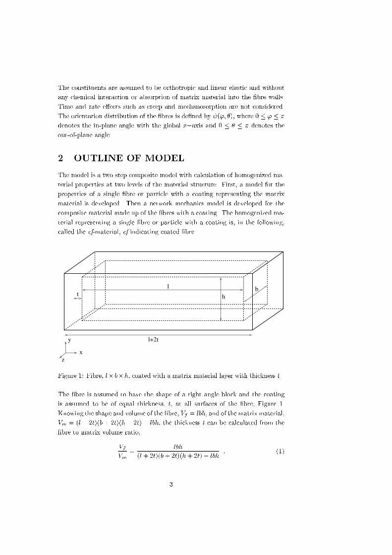
The constituents are assumed to be orthotropic and linear elastic and without

any chemical interaction or absorption of matrix material into the �bre walls.

Time and rate e�ects such as creep and mechanosorption are not considered.

The orientation distribution of the �bres is de�ned by ('; �), where 0 � ' � �

denotes the in-plane angle with the global x�axis and 0 � � � � denotes the

out-of-plane angle.

2 OUTLINE OF MODEL

The model is a two-step composite model with calculation of homogenized ma-

terial properties at two levels of the material structure. First, a model for the

properties of a single �bre or particle with a coating representing the matrix

material is developed. Then a network mechanics model is developed for the

composite material made up of the �bres with a coating. The homogenized ma-

terial representing a single �bre or particle with a coating is, in the following,

called the cf-material, cf indicating coated �bre.

b

z

y

x

l+2t

l

ht

Figure 1: Fibre, l� b�h, coated with a matrix material layer with thickness t.

The �bre is assumed to have the shape of a right angle block and the coating

is assumed to be of equal thickness, t, at all surfaces of the �bre, Figure 1.

Knowing the shape and volume of the �bre, Vf = lbh, and of the matrix material,

Vm = (l + 2t)(b + 2t)(h+ 2t)� lbh, the thickness t can be calculated from the

�bre to matrix volume ratio,

VfVm

=lbh

(l + 2t)(b+ 2t)(h+ 2t)� lbh: (1)

3

The total volume is Vtot = Vf + Vm + Vp , where Vp is the volume of possible

pores. The �bre volume fraction is

vf =VfVtot

: (2)

The properties of the cf-material are in general orthotropic due to the more or

less oblong shape of the �bre and due to orthotropic properties of the �bre. The

homogenised properties of the composite material are obtained by integration

over the �bre orientation directions. This integration is made with respect to a

function containing the properties of the cf-material. This function has a free

parameter, �;�1 � � � 1, such that � = 1 corresponds to the extreme of

parallel coupling with complete interaction and equal strain for the variously

oriented cf-material, and � = �1 corresponds to the extreme of series couplingwith equal stress. Two types of functions of � are studied: a linear function

and an exponential function.

3 HOMOGENISATION OF COATED FIBRE

The general principle used for calculating the properties of the homogenous

cf-material is that the response to load and to moisture change should be the

same in terms of deformation of the cf-material and the coated �bre composite

structure. In the present analysis the response of the composite structure is de-

termined by minimization of potential energy. This minimization is carried out

to a �nite number of parameters, degrees of freedom, which, together with an

assumption regarding the shape of the deformed structure, de�nes the strains.

The present choice of shape functions ful�lls the conditions of compatibility.

Hence the calculated sti�ness of the structure will, in general, somewhat over-

estimate the true sti�ness. The deformed shape valid for loading by normal

force in the x�; y� or z�direction and for the change of moisture content is,

for the 3D case, de�ned by 3 times 2 normal strain parameters, see Figure 2b.

The shape for shear loadings is de�ned by 3 times 3 independent shear strain

parameters, see Figure 2c.

4

f

γ

γ

m3

m2

m1γ

γ

P

a)

c)

P

P’ P’

y t

t

b

x

P

b)

x2ε

x1

P x1ε

ε

Figure 2: Shape of coated �bre, a) unloaded, b) loaded in tension, c) loaded in

shear.

The potential energy for a structure or body and the loads acting on the body

is

� = U �W =1

2

ZV

"T�dV �

ZS

uTfdS (3)

where U is the strain energy and W is the potential energy of the loads. Mini-

mization of � with respect to the free parameters

@�

@"0= 0; (4)

provides the equations from which the free strain parameters can be calculated.

3.1 E-moduli and Poissons ratios of cf-material

The sti�ness properties of the homogenized cf-material are de�ned by a 6 � 6

compliance matrix, Ccf , relating a stress vector and a strain vector " = Ccf �

in the local coordinate system of the cf

5

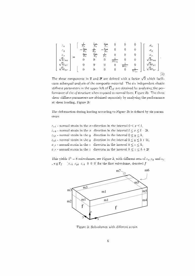
2666666664

"x

"y

"zp2"xyp2"xzp2"yz

3777777775=

26666666664

1Ex

� �yxEy

� �zxEz

0 0 0

� �xyEx

1Ey

� �zyEz

0 0 0

� �xzEx

� �yzEy

1Ez

0 0 0

0 0 0 12Gxy

0 0

0 0 0 0 12Gxz

0

0 0 0 0 0 12Gyz

37777777775

2666666664

�x

�y

�zp2�xyp2�xzp2�yz

3777777775:

(5)

The shear components in " and � are de�ned with a factorp2 which facili-

tates subsequal analysis of the composite material. The six independent elastic

sti�ness parameters in the upper left of Ccf are obtained by analysing the per-

formance of the cf structure when exposed to normal force, Figure 2b. The three

shear sti�ness parameters are obtained separately by analysing the performance

at shear loading, Figure 2c.

The deformation during loading according to Figure 2b is de�ned by six param-

eters:

"x1 - normal strain in the x�direction in the interval 0 � x � l,

"x2 - normal strain in the x�direction in the interval l � x � l + 2t,

"y1 - normal strain in the y�direction in the interval 0 � y � b,

"y2 - normal strain in the y�direction in the interval b � y � b+ 2t,

"z1 - normal strain in the z�direction in the interval 0 � z � h,

"z2 - normal strain in the z�direction in the interval h � z � h+ 2t.

This yields 23 = 8 subvolumes, see Figure 3, with di�erent sets of "x; "y and "z

, e.g "f = [ "x1 "y1 "z1 0 0 0] for the �rst subvolume, denoted f .

m7

m5

m4

m3

f

m1m2

m5

x

z

y

m6

m1

m1

m3

f

Figure 3: Subvolumes with di�erent strain.

6

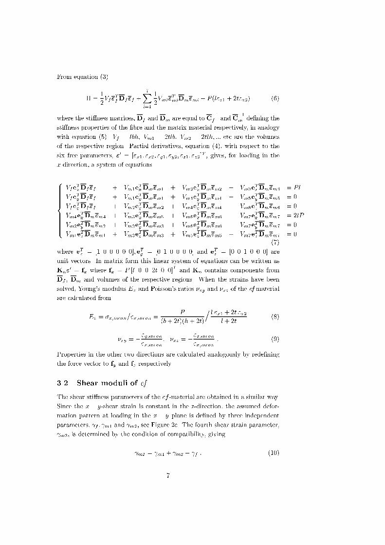
From equation (3)

� =1

2Vf"

TfDf"f +

7Xi=1

1

2Vmi"

TmiDm"mi � P (l"x1 + 2t"x2) (6)

where the sti�ness matrices, Df andDm are equal to C�1f and C

�1m de�ning the

sti�ness properties of the �bre and the matrix material respectively, in analogy

with equation (5). Vf = lbh; Vm1 = 2tlb; Vm2 = 2tlh; ::: etc are the volumes

of the respective region. Partial derivatives, equation (4), with respect to the

six free parameters, "0 = ["x1; "x2; "y1; "y2; "z1; "z2]T , gives, for loading in the

x-direction, a system of equations

8>>>>>>>><>>>>>>>>:

VfeTxDf"f + Vm1e

TxDm"m1 + Vm2e

TxDm"m2 + Vm3e

TxDm"m3 = P l

VfeTyDf"f + Vm1e

TyDm"m1 + Vm4e

TyDm"m4 + Vm5e

TyDm"m5 = 0

VfeTzDf"f + Vm2e

TzDm"m2 + Vm4e

TzDm"m4 + Vm6e

TzDm"m6 = 0

Vm4eTxDm"m4 + Vm5e

TxDm"m5 + Vm6e

TxDm"m6 + Vm7e

TxDm"m7 = 2tP

Vm2eTyDm"m2 + Vm3e

TyDm"m3 + Vm6e

TyDm"m6 + Vm7e

TyDm"m7 = 0

Vm1eTzDm"m1 + Vm3e

TzDm"m3 + Vm5e

TzDm"m5 + Vm7e

TzDm"m7 = 0

(7)

where eTx = [1 0 0 0 0 0]; eTy = [0 1 0 0 0 0] and eTz = [0 0 1 0 0 0] are

unit vectors. In matrix form this linear system of equations can be written as

Kn"0 = fx where fx = P [l 0 0 2t 0 0]

Tand Kn contains components from

Df , Dm and volumes of the respective regions. When the strains have been

solved, Young's modulus Ex and Poisson's ratios �xy and �xz of the cf-material

are calculated from

Ex = �x;mean/"x;mean =P

(b+ 2t)(h+ 2t)/ l "x1 + 2t "x2

l + 2t(8)

�xy = �"y;mean

"x;mean; �xz = � "z;mean

"x;mean: (9)

Properties in the other two directions are calculated analogously by rede�ning

the force vector to fy and fz respectively.

3.2 Shear moduli of cf

The shear sti�ness parameters of the cf -material are obtained in a similar way.

Since the x � y-shear strain is constant in the z-direction, the assumed defor-

mation pattern at loading in the x � y plane is de�ned by three independent

parameters, f ; m1 and m2, see Figure 2c. The fourth shear strain parameter,

m3, is determined by the condition of compatibility, giving

m3 = m1 + m2 � f : (10)

7

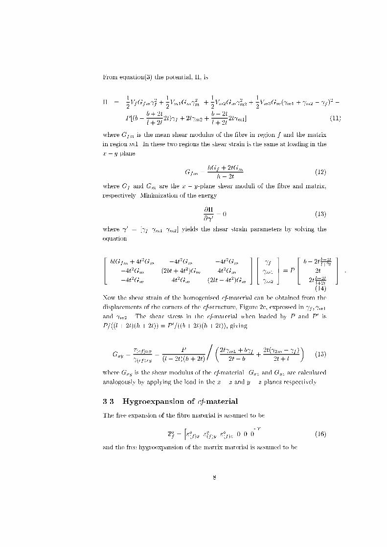
From equation(3) the potential, �, is

� =1

2VfGfm

2f +

1

2Vm1Gm

2m1 +

1

2Vm2Gm

2m2 +

1

2Vm3Gm( m1 + m2 � f )

2 �

P [(b� b+ 2t

l + 2t2t) f + 2t m2 +

b+ 2t

l + 2t2t m1] (11)

where Gfm is the mean shear modulus of the �bre in region f and the matrix

in region m1. In these two regions the shear strain is the same at loading in the

x� y plane.

Gfm =hGf + 2tGm

h+ 2t(12)

where Gf and Gm are the x � y-plane shear moduli of the �bre and matrix,

respectively. Minimization of the energy

@�

@ 0= 0 (13)

where 0 = [ f m1 m2] yields the shear strain parameters by solving the

equation

264blGfm + 4t2Gm �4t2Gm �4t2Gm

�4t2Gm (2bt+ 4t2)Gm 4t2Gm

�4t2Gm 4t2Gm (2lt+ 4t2)Gm

375264

f

m1

m2

375 = P

264b� 2t b+2t

l+2t

2t

2t b+2tl+2t

375 :

(14)

Now the shear strain of the homogenised cf-material can be obtained from the

displacements of the corners of the cf-structure, Figure 2c, expressed in f ; m1

and m2. The shear stress in the cf-material when loaded by P and P 0 is

P=((l + 2t)(h+ 2t)) = P 0=((b+ 2t)(h+ 2t)), giving

Gxy =�(cf)xy

(cf)xy=

P

(l + 2t)(h+ 2t)/�2t m1 + b f

2t+ b+2t( 2m � f )

2t+ l

�(15)

where Gxy is the shear modulus of the cf-material. Gxz and Gyz are calculated

analogously by applying the load in the x� z and y � z planes respectively.

3.3 Hygroexpansion of cf-material

The free expansion of the �bre material is assumed to be

"of =

h"o(f)x "o(f)y "o(f)z 0 0 0

iT(16)

and the free hygroexpansion of the matrix material is assumed to be

8

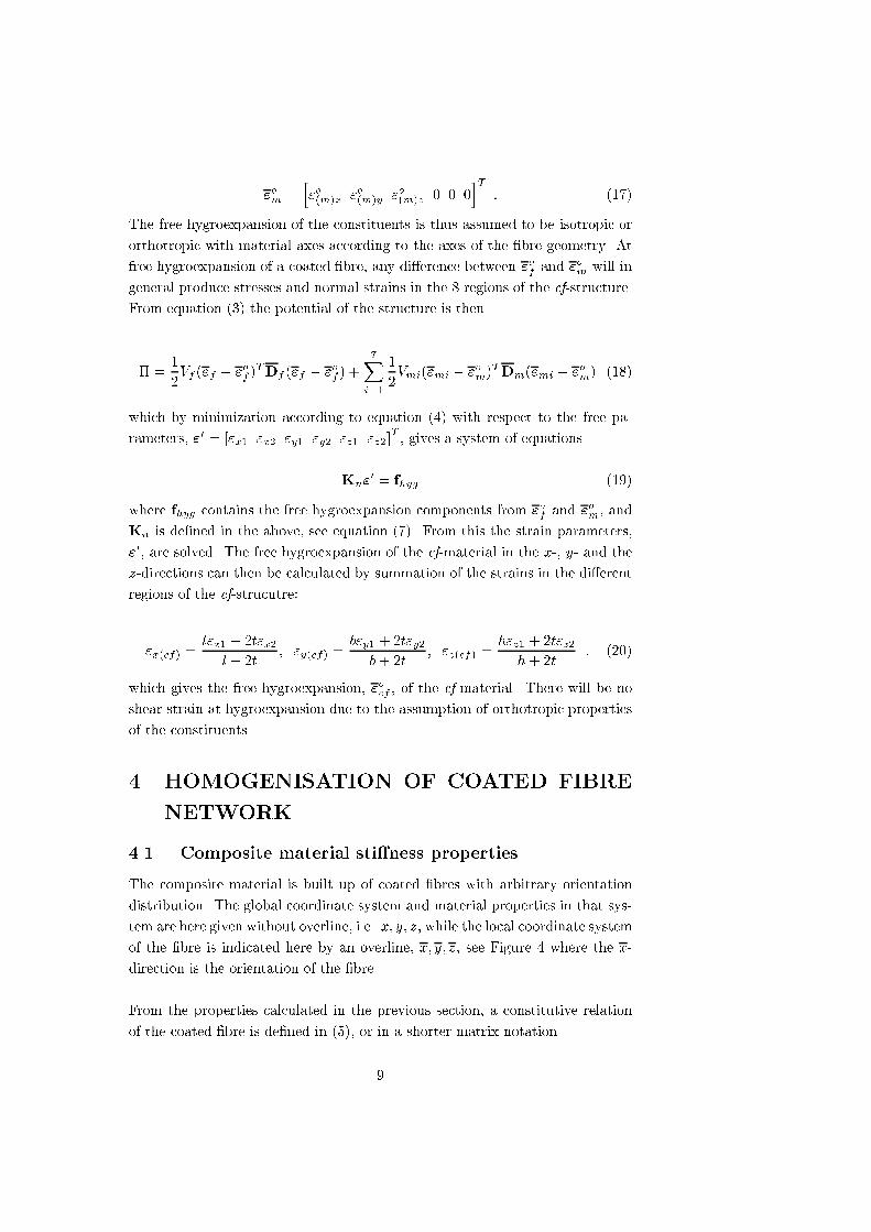
"om =

h"o(m)x "o(m)y "o(m)z 0 0 0

iT: (17)

The free hygroexpansion of the constituents is thus assumed to be isotropic or

orthotropic with material axes according to the axes of the �bre geometry. At

free hygroexpansion of a coated �bre, any di�erence between "of and "om will in

general produce stresses and normal strains in the 8 regions of the cf-structure.

From equation (3) the potential of the structure is then

� =1

2Vf ("f � "

of )TDf ("f � "

of ) +

7Xi=1

1

2Vmi("mi � "

om)

TDm("mi � "

om) (18)

which by minimization according to equation (4) with respect to the free pa-

rameters, "0 = ["x1 "x2 "y1 "y2 "z1 "z2]T , gives a system of equations

Kn"0 = fhyg (19)

where fhyg contains the free hygroexpansion components from "of and "om, and

Kn is de�ned in the above, see equation (7). From this the strain parameters,

"0, are solved. The free hygroexpansion of the cf-material in the x-, y- and the

z-directions can then be calculated by summation of the strains in the di�erent

regions of the cf-strucutre:

"x(cf) =l"x1 + 2t"x2

l+ 2t; "y(cf) =

b"y1 + 2t"y2b+ 2t

; "z(cf) =h"z1 + 2t"z2

h+ 2t: (20)

which gives the free hygroexpansion, "ocf , of the cf-material. There will be no

shear strain at hygroexpansion due to the assumption of orthotropic properties

of the constituents.

4 HOMOGENISATION OF COATED FIBRE

NETWORK

4.1 Composite material sti�ness properties

The composite material is built up of coated �bres with arbitrary orientation

distribution. The global coordinate system and material properties in that sys-

tem are here given without overline, i.e. x; y; z, while the local coordinate system

of the �bre is indicated here by an overline, x; y; z, see Figure 4 where the x-

direction is the orientation of the �bre.

From the properties calculated in the previous section, a constitutive relation

of the coated �bre is de�ned in (5), or in a shorter matrix notation

9

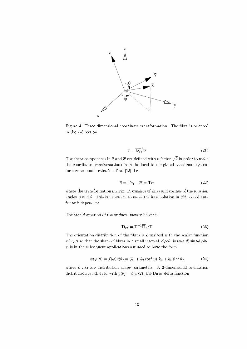
ϕ

θ

y

x

y

x

zz

Figure 4: Three dimensional coordinate transformation. The �bre is oriented

in the x-direction.

" = D�1cf � (21)

The shear components in " and � are de�ned with a factorp2 in order to make

the coordinate transformations from the local to the global coordinate system

for stresses and strains identical [15], i.e.

" = T"; � = T� (22)

where the transformation matrix, T, consists of sines and cosines of the rotation

angles ' and �. This is necessary to make the interpolation in (28) coordinate

frame independent.

The transformation of the sti�ness matrix becomes

Dcf = T�1DcfT (23)

The orientation distribution of the �bres is described with the scalar function

('; �) so that the share of �bres in a small interval, d'd�, is ('; �) sin �d'd�.

is in the subsequent applications assumed to have the form

('; �) = f(')g(�) = (k1 + k2 cos2 ')(k3 + k4 sin

2 �) (24)

where k1::k4 are distribution shape parameters. A 2-dimensional orientation

distribution is achieved with g(�) = �(�=2), the Dirac delta function.

10

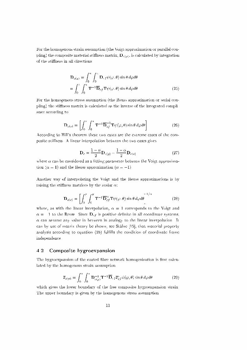
For the homogenous strain assumption (the Voigt approximation or parallel cou-

pling) the composite material sti�ness matrix,Dc(p), is calculated by integration

of the sti�ness in all directions

Dc(p) =

Z �

0

Z �

0

Dcf ('; �) sin � d'd�

=

Z �

0

Z �

0

T�1DcfT ('; �) sin � d'd� (25)

For the homogenous stress assumption (the Reuss approximation or serial cou-

pling) the sti�ness matrix is calculated as the inverse of the integrated compli-

ance according to

Dc(s) =

�Z �

0

Z �

0

T�1D

�1

cf T ('; �) sin � d'd�

��1

(26)

According to Hill's theorem these two cases are the extreme cases of the com-

posite sti�ness. A linear interpolation between the two cases gives

Dc =1 + �

2Dc(p) +

1� �

2Dc(s) (27)

where � can be considered as a �tting parameter between the Voigt approxima-

tion (� = 1) and the Reuss approximation (� = �1).

Another way of interpolating the Voigt and the Reuss approximations is by

raising the sti�ness matrices by the scalar �:

Dc(s) =

�Z �

0

Z �

0

T�1D�cfT ('; �) sin � d'd�

�1=�(28)

where, as with the linear interpolation, � = 1 corresponds to the Voigt and

� = �1 to the Reuss. Since Dcf is positive de�nite in all coordinate systems,

� can assume any value in between in analogy to the linear interpolation. It

can by use of matrix theory be shown, see St�alne [15], that material property

analysis according to equation (28) ful�lls the condition of coordinate frame

independence.

4.2 Composite hygroexpansion

The hygroexpansion of the coated �bre network homogenisation is �rst calcu-

lated by the homogenous strain assumption

"c(p) =

Z �

0

Z �

0

D�1c(p)T

�1Dcf"

ocf ('; �) sin � d'd� (29)

which gives the lower boundary of the free composite hygroexpansion strain.

The upper boundary is given by the homogenous stress assumption

11

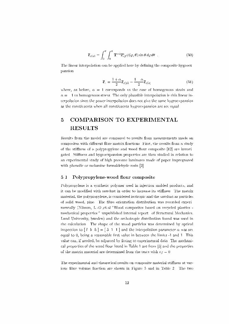
"c(s) =

Z �

0

Z �

0

T�1"ocf ('; �) sin � d'd� : (30)

The linear interpolation can be applied here by de�ning the composite hygroex-

pansion

"c =1 + �

2"c(p) +

1� �

2"c(s) (31)

where, as before, � = 1 corresponds to the case of homogenous strain and

� = �1 to homogenous stress. The only plausible interpolation is this linear in-terpolation since the power interpolation does not give the same hygroexpansion

as the constituents when all constituents hygroexpansion are set equal.

5 COMPARISON TO EXPERIMENTAL

RESULTS

Results from the model are compared to results from measurements made on

composites with di�erent �bre-matrix fractions. First, the results from a study

of the sti�ness of a polypropylene and wood our composite [12] are investi-

gated. Sti�ness and hygroexpansion properties are then studied in relation to

an experimental study of high pressure laminates made of paper impregnated

with phenolic or melamine formaldehyde resin [2].

5.1 Polypropylene-wood our composite

Polypropylene is a synthetic polymer used in injection molded products, and

it can be modi�ed with sawdust in order to increase its sti�ness. The matrix

material, the polypropylene, is considered isotropic and the sawdust as particles

of solid wood, pine. The �bre orientation distribution was recorded experi-

mentally (Nilsson, L.-O.,et.al."Wood composites based on recycled plastics -

mechanical properties." unpublished internal report. of Structural Mechanics,

Lund University, Sweden) and the orthotropic distribution found was used in

the calculation. The shape of the wood particles was determined by optical

inspection to [ l b h ] = [ 3 1 1 ] and the interpolation parameter � was set

equal to 0, being a reasonable �rst value in between the limits -1 and 1. This

value can, if needed, be adjusted by �tting to experimental data. The mechani-

cal properties of the wood our listed in Table 1 are from [5] and the properties

of the matrix material are determined from the tests with vf = 0.

The experimental and theoretical results on composite material sti�ness at var-

ious �bre volume fraction are shown in Figure 5 and in Table 2. The two

12

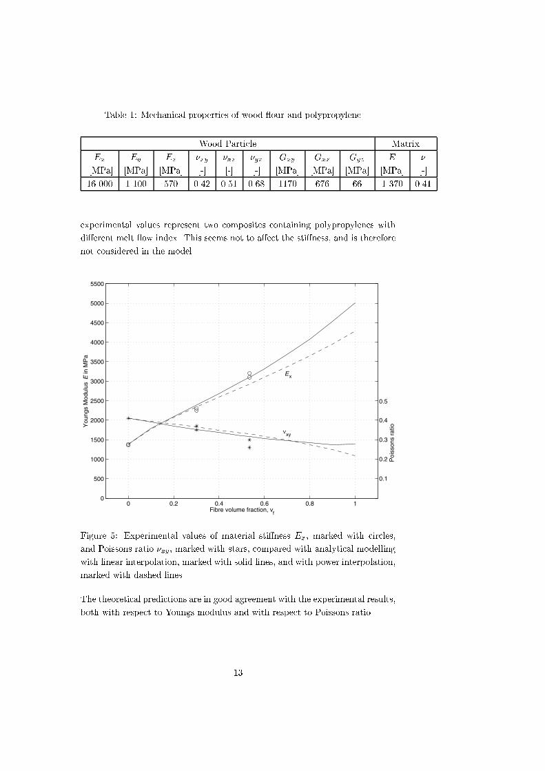
Table 1: Mechanical properties of wood our and polypropylene.

Wood Particle Matrix

Ex Ey Ez �xy �xz �yz Gxy Gxz Gyz E �

[MPa] [MPa] [MPa] [-] [-] [-] [MPa] [MPa] [MPa] [MPa] [-]

16 000 1 100 570 0.42 0.51 0.68 1170 676 66 1 370 0.41

experimental values represent two composites containing polypropylenes with

di�erent melt ow index. This seems not to a�ect the sti�ness, and is therefore

not considered in the model.

0 0.2 0.4 0.6 0.8 10

500

1000

1500

2000

2500

3000

3500

4000

4500

5000

5500

Fibre volume fraction, vf

xy

x

ν

You

ngs

Mod

ulus

E

E in M

Pa

0.1

0.2

0.3

0.4

0.5

Poi

sson

s ra

tio

Figure 5: Experimental values of material sti�ness Ex, marked with circles,

and Poissons ratio �xy, marked with stars, compared with analytical modelling

with linear interpolation, marked with solid lines, and with power interpolation,

marked with dashed lines.

The theoretical predictions are in good agreement with the experimental results,

both with respect to Youngs modulus and with respect to Poissons ratio.

13

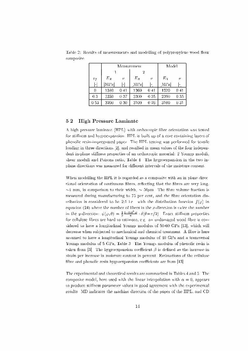
Table 2: Results of measurements and modelling of polypropylene-wood our

composite.

Measurement Model

1 2

vf EX � EX � EX �

[-] [MPa] [-] [MPa] [-] [MPa] [-]

0 1380 0.41 1360 0.41 1370 0.41

0.3 2250 0.37 2300 0.35 2390 0.35

0.53 3200 0.30 3100 0.26 3100 0.31

5.2 High Pressure Laminate

A high pressure laminate (HPL) with orthotropic �bre orientation was tested

for sti�ness and hygroexpansion. HPL is built up of a core containing layers of

phenolic resin-impregnated paper. The HPL testing was performed for tensile

loading in three directions [2], and resulted in mean values of the four indepen-

dent in-plane sti�ness properties of an orthotropic material: 2 Youngs moduli,

shear moduli and Poisons ratio, Table 4. The hygroexpansion in the two in-

plane directions was measured for di�erent intervals of the moisture content.

When modelling the HPL it is regarded as a composite with an in-plane direc-

tional orientation of continuous �bres, re ecting that the �bres are very long,

�1 mm, in comparison to their width, � 50�m. The �bre volume fraction is

measured during manufacturing to 75 per cent, and the �bre orientation dis-

tribution is considered to be 2:1 i.e. with the distribution function f(') in

equation (24) where the number of �bres in the x-direction is twice the number

in the y-direction: ('; �) = 231+cos2 '

� � �(�=�=2). Exact sti�ness properties

for cellulose �bres are hard to estimate, e.g. an undamaged wood �bre is con-

sidered to have a longitudinal Youngs modulus of 50-60 GPa [13], which will

decrease when subjected to mechanical and chemical treatment. A �bre is here

assumed to have a longitudinal Youngs modulus of 40 GPa and a transversal

Youngs modulus of 5 GPa, Table 3. The Youngs modulus of phenolic resin is

taken from [3]. The hygroexpansion coe�cient � is de�ned as the increase in

strain per increase in moisture content in percent. Estimations of the cellulose

�bre and phenolic resin hygroexpansion coe�cients are from [13].

The experimental and theoretical results are summarized in Tables 4 and 5. The

composite model, here used with the linear interpolation with � = 0, appears

to produce sti�ness parameter values in good agreement with the experimental

results. MD indicates the machine direction of the paper of the HPL, and CD

14

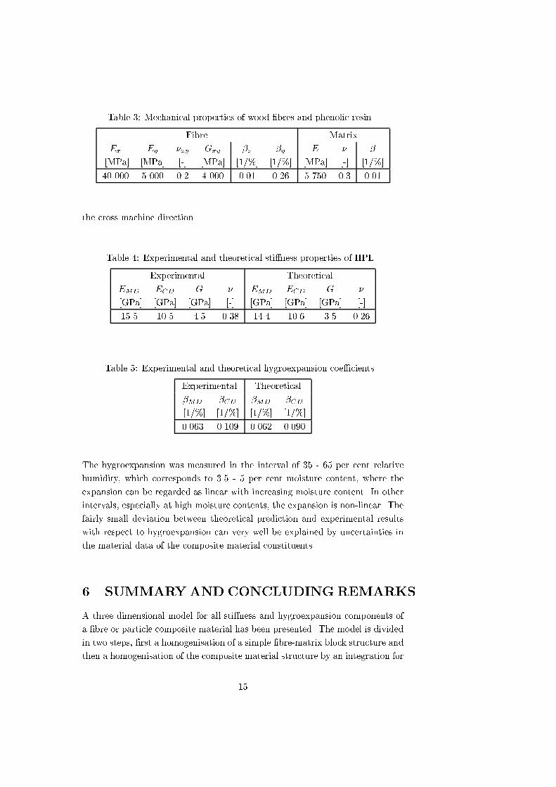
Table 3: Mechanical properties of wood �bres and phenolic resin.

Fibre Matrix

Ex Ey �xy Gxy �x �y E � �

[MPa] [MPa] [-] [MPa] [1/%] [1/%] [MPa] [-] [1/%]

40 000 5 000 0.2 4 000 0.01 0.26 5 750 0.3 0.01

the cross machine direction.

Table 4: Experimental and theoretical sti�ness properties of HPL.

Experimental Theoretical

EMD ECD G � EMD ECD G �

[GPa] [GPa] [GPa] [-] [GPa] [GPa] [GPa] [-]

15.5 10.5 4.5 0.38 14.4 10.6 3.5 0.26

Table 5: Experimental and theoretical hygroexpansion coe�cients.

Experimental Theoretical

�MD �CD �MD �CD

[1/%] [1/%] [1/%] [1/%]

0.063 0.109 0.062 0.090

The hygroexpansion was measured in the interval of 35 - 65 per cent relative

humidity, which corresponds to 3.5 - 5 per cent moisture content, where the

expansion can be regarded as linear with increasing moisture content. In other

intervals, especially at high moisture contents, the expansion is non-linear. The

fairly small deviation between theoretical prediction and experimental results

with respect to hygroexpansion can very well be explained by uncertainties in

the material data of the composite material constituents.

6 SUMMARYANDCONCLUDING REMARKS

A three dimensional model for all sti�ness and hygroexpansion components of

a �bre or particle composite material has been presented. The model is divided

in two steps, �rst a homogenisation of a simple �bre-matrix block structure and

then a homogenisation of the composite material structure by an integration for

15

all �bre directions. The homogenisation of the coated �bre is obtained by ap-

plying normal and shear forces one by one in various directions and computing

the strains by a minimization of the potential energy. Normal sti�nesses, Pois-

sons ratios and shear sti�nesses are then determined from de�nition. Thereby

the whole sti�ness matrix can be expressed in terms of the properties of the

constituents and the shape of �bre or particle.

The composite material sti�ness is �rst obtained for the two extremes of ho-

mogenous strain and homogenous stress. This is done by integration of the sti�-

ness or compliance matrix of the coated �bre material for all �bre directions.

Analysis of the hygroexpansion properties of a coated �bre and the composite

material was carried out consistent with the sti�ness analysis.

Interpolation between the two extreme cases of homogenous strain and homoge-

nous stress can be done by a simple linear weighting of the sti�ness matrices

or by an exponential weighting. Both interpolations have the quality of co-

ordinate invariance. When comparing the di�erent procedures, the exponetial

approach is more appealing from a mathematial point of view, since it is unam-

biguous. However, the linear interpolation is simpler, more numerically stable

and demands fewer calculations. When calculating the hygroexpansion the lin-

ear interpolation is the only way possible. The two interpolations appear to give

fairly similar results.

The resulting sti�ness matrix for the composite material is symmetric, valid

in the entire range between 0 per cent and 100 per cent �bre content, and co-

incident with the exact solutions that exist for the extreme cases of laminate

geometries and continuous-�bre systems with equal shear rigidities. At this

stage, only time-independent properties of the constituents are considered in

the model. Consideration of varying �bre lengths according a �bre length dis-

tribution would be easy to implement. The present model comprise some rather

extensive equations. Such qualities can however be dealt with in a convenient

manner by use of MAPLE [11] or any other similair computer code.

Comparisons between the model and measurements gave a good agreement in

sti�nesses and Poissons ratio. When comparing with the measured hygroexpan-

sion coe�cients, the calculated hygroexpansion coe�cients are slightly lower.

The comparison to experimental results were here made only for two types of

material and it can not be generally concluded that the theoretical model un-

derestimates hygroexpansion. The model presented is exible in such manner

that it can be used in a number of di�erent applications and contribute to a

better understanding of composite material behaviour.

16

7 ACKNOWLEDGEMENT

This work was �nanced by the Swedish Wood Technology Research Colleague.

17

APPENDIX I.

References

[1] Aboudi, J. (1991). "Mechanics of Composite Materials", Elsevier, Amster-

dam, The Netherlands, 14-18.

[2] Andersson, B. (1999). "Composite materials' hygro-mechanical properties",

Masters thesis, Report TVSM-3018, Div. of Structural Mechanics, Lund

University, Sweden.

[3] Barth, Th. (1984). "Der Ein uss der Feuchteaufnahme auf die mechanis-

chen Eigenschaften von Phenolplasten." Z. Werksto�tech, Verlag Chemie,

Weinheim, Germany, 15, 299-308.

[4] Cox, H. L. (1951). "The elasticity and strength of paper and other �brous

materials." Brittish J. Appl. Phys., London, 3, 72-79.

[5] Dinwoodie, J. M. (1989). Wood: nature's cellular, polymeric �bre-

composite, The Institute of Metals, London, 57.

[6] Dunn, M. L., Ledbetter, H., Heyliger, P. R. and Choi, C. S. (1996). "Elas-

tic constants of textured short-�ber composites." J. Mech. Phys. Solids,

Elsevier, Amsterdam, The Netherlands, 44, 1509-1541.

[7] Fu, S.-Y. Lauke, B. (1998). "An analytical characterization of the

anisotropy of the elastic modulus of misaligned short-�ber-reinforced poly-

mers." Composites Sci. Techn., Elsevier, Amsterdam, The Netherlands, 58,

1961-1972.

[8] Halpin, J. C., Kardos, J. L. (1976). "The Halpin-Tsai equations: A review."

Polym. Eng. Sci., Swets, 16, 344-352.

[9] Hashin, Z., Shtrikman, S. (1963). "A variational approach to the theory

of the elastic behaviour of multiphased materials." J. Mech. Phys. Solids,

Elsevier, Amsterdam, The Netherlands, 11, 127-140.

[10] Heyden, S. (2000). Network modelling for the evaluation of mechanical

properties of cellulose �bre u�., Doctoral thesis, Report TVSM-1011, Div.

of Structural Mechanics, Lund University, Sweden.

[11] MAPLE (2000), "A symbolic computation system or computer algebra

system", Version 6.0, Waterloo Maple, Inc.

18

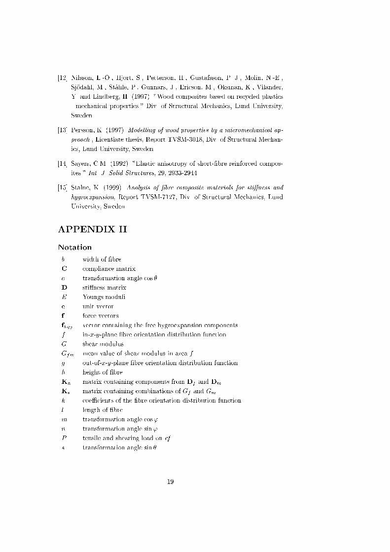
[12] Nilsson, L.-O., Hjort, S., Petterson, H., Gustafsson, P. J., Molin, N.-E.,

Sj�odahl, M., St�ahle, P., Gunnars, J., Ericson, M., Oksman, K., Vilander,

Y. and Lindberg, H. (1997). "Wood composites based on recycled plastics

- mechanical properties." Div. of Structural Mechanics, Lund University,

Sweden.

[13] Persson, K. (1997). Modelling of wood properties by a micromechanical ap-

proach., Licentiate thesis, Report TVSM-3018, Div. of Structural Mechan-

ics, Lund University, Sweden.

[14] Sayers, C.M. (1992). "Elastic anisotropy of short-�bre reinforced compos-

ites." Int. J. Solid Structures, 29, 2933-2944.

[15] St�alne, K. (1999). Analysis of �bre composite materials for sti�ness and

hygroexpansion, Report TVSM-7127, Div. of Structural Mechanics, Lund

University, Sweden.

APPENDIX II.

Notation

b width of �bre

C compliance matrix

c transformation angle cos �

D sti�ness matrix

E Youngs moduli

e unit vector

f force vectors

fhyg vector containing the free hygroexpansion components

f in-x-y-plane �bre orientation distribution function

G shear modulus

Gfm mean value of shear modulus in area f

g out-of-x-y-plane �bre orientation distribution function

h height of �bre

Kn matrix containing components from Df and Dm

Ks matrix containing combinations of Gf and Gm

k coe�cients of the �bre orientation distribution function

l length of �bre

m transformation angle cos'

n transformation angle sin'

P tensile and shearing load on cf

s transformation angle sin �

19

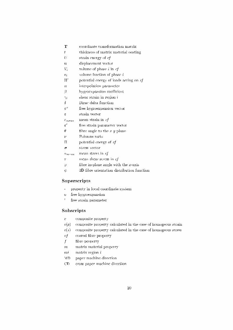
T coordinate transformation matrix

t thickness of matrix material coating

U strain energy of cf

u displacement vector

Vi volume of phase i in cf

vi volume fraction of phase i

W potential energy of loads acting on cf

� interpolation parameter

� hygroexpansion coe�cient

i shear strain in region i

� Dirac delta function

"o free hygroexpansion vector

" strain vector

"mean mean strain in cf

"0 free strain parameter vector

� �bre angle to the x-y-plane

� Poissons ratio

� potential energy of cf

� stress vector

�mean mean stress in cf

� mean shear stress in cf

' �bre in-plane angle with the x-axis

3D �bre orientation distribution function

Superscripts

- property in local coordinate system

o free hygroexpansion

' free strain parameter

Subscripts

c composite property

c(p) composite property calculated in the case of homogeous strain

c(s) composite property calculated in the case of homogeous stress

cf coated �bre property

f �bre property

m matrix material property

mi matrix region i

MD paper machine direction

CD cross paper machine direction

20

IV

A 3D Finite Element Fibre Network

Model for Composite Material Sti�ness

and Hygroexpansion Analysis

Kristian St�alne and Per Johan Gustafsson

Division of Structural Mechanics

Lund University, Sweden

A 3D Finite Element Fibre Network Model

for Composite Material Sti�ness and

Hygroexpansion Analysis

Kristian St�alne and Per Johan Gustafsson

Abstract

A 3D �nite element �bre network model was developed to be used as a tool

for predicting the sti�ness and the hygroexpansion properties of �bre composite

materials, such as high pressure laminates. The wood �bres are modelled as

orthotropic or transversely isotropic solid elements surrounded by an isotropic

matrix material. The �bres and the matrix are arranged in a unit cell subjected

to loading or changes in moisture content. The constitutive parameters of the

homogenised composite material are obtained by simulating the response of the

composite structure to load and moisture. The model is evaluated by comparing

the results it provides with various experimental results and with results of

a recent analytical model and of various parameter studies. The model also

provides in addition to properties of the homogenised material considerable

information concerning stresses and strains within the material structure.

1

1 Introduction

High pressure laminate, HPL, is a wood �bre composite whose usage has in-

creased much during the recent decades. It is composed of craft paper impreg-

nated by phenolic or melamine resin. A key issue concerning wood composites is

that of shape stability in relation to a moisture content gradient or to a change

in moisture content. This entails the need for methods enabling the hygroex-

pansion and sti�ness properties of wood composites such as HPL to be analysed

and predicted.

Several analytical models for the sti�ness of composite materials have been

developed in recent decades [11, 22]. Many of these are based on the homogeni-

sation of a single �bre surrounded by matrix material [1, 9]. These models

assumes there to be no interaction between the �bres. Such an assumption is

questionable in connection with HPL, however, since the particle phase of this

composite material is paper, which is a network of long �bres bonded to each

other.

Developments in the area of numerical simulation as based on the �nite element

method, for example, have made it possible to model more complicated �bre

composite material structures, consisting of more than one �bre [7, 4, 6, 10, 24].

Most of these studies have dealt with estimation of the sti�ness properties of

plane fabric composites. These materials have a weaved �bre phase in which

the �bres are crossed over and under each other at right angles [20, 8, 23, 13].

Since the fabric geometry is regular, homogenisation of a single �bre crossing

is su�cient to provide a satisfactory estimate of the composite material sti�-

ness. Composites with �bre networks of a more random types of have also been

studied, using numerical simulations [15, 17, 19, 21]. There has been no study

at a micro mechanical level, however, of the behaviour of composite materials

of irregular geometry. Little appears to have been done either regarding sim-

ulation of the hygroexpansion or thermal expansion properties of such materials.

The aim of the model discussed is to simulate the mechanical behaviour of a

wood �bre composite with an irregular �bre network, such that of paper. The

model is a �nite element 3D model using a square unit cell in which there are

a number of �bres modelled as orthotropic solid elements surrounded by an

isotropic matrix material. The response of the unit cell when exposed to an

increase in moisture content and to loading in the x-, y- and z-direction, respec-

tively, is simulated. The parameters of the model are the mechanical properties

of the constituents, the �bre geometry, the �bre orientation distribution and the

�bre volume fractions. The geometry of the �bres is created in a preprocessor

allowing the user to decide on the location of each �bre. This enables a good rep-

2

resentation of the micro-structure of the �bre composite material to be obtained.

The numerical results concern primarily the in uence of the model parame-

ters on the sti�ness and the hygroexpansion of the homogenised material. The

predicted properties are compared with the results of a recently developed ana-

lytical model [18] and with certain test results. In addition to the homogenised

material properties, the model provides considerably information on the magni-

tude and distribution of the stresses and strains within the material structure.

This can provide estimates of the risk for development of micro-cracks, damage,

creep or permanent plastic deformation within the material structure when ex-

posed to various loads or moisture actions.

2 Description of the Model

The model concerns sti�ness and hygroexpansion properties. Sti�ness is anal-

ysed by exposing a square unit cell containing a number of wood �bres and a

�lling of matrix material to a given deformation in one direction and to zero

load in all other directions. The sti�ness tensor of the unit composite cell can

be obtained by calculating the mean values of the stress and strain vectors for

the volume of the cell. The hygroexpansion parameters of the composite cell

are obtained by simulating an increase in moisture content and calculating the

average strain of the unit cell in each direction.

The numerical modelling involves four steps: modelling the �bre geometry, �nite

element modelling, solution of the system of equations and postprocessing the

results. The �bre and network geometry is created by a preprocessor written in

Matlab-code [14]. It de�nes the volumes of the �bres and of the matrix material

and generates input data to the commercial preprocessor Patran, in which the

�nite element mesh is created, material properties are assigned and the load

cases are de�ned. The �nite element analysis is performed by an Abaqus solver,

the postprocessing being done using Patran.

2.1 General assumptions

The cross section of the �bres is assumed to be rectangular in shape, correspond-

ing approximately to the shape of the collapsed wood �bres that the paper is

made of. The height and the width of the �bres are assumed to be constant and

to be the same for all the �bres, which are considered to be long and slender, no

�bre ending in the cell. The space within the unit cell not occupied by �bres is

occupied completely by matrix material. Thus voids are not considered in the

3

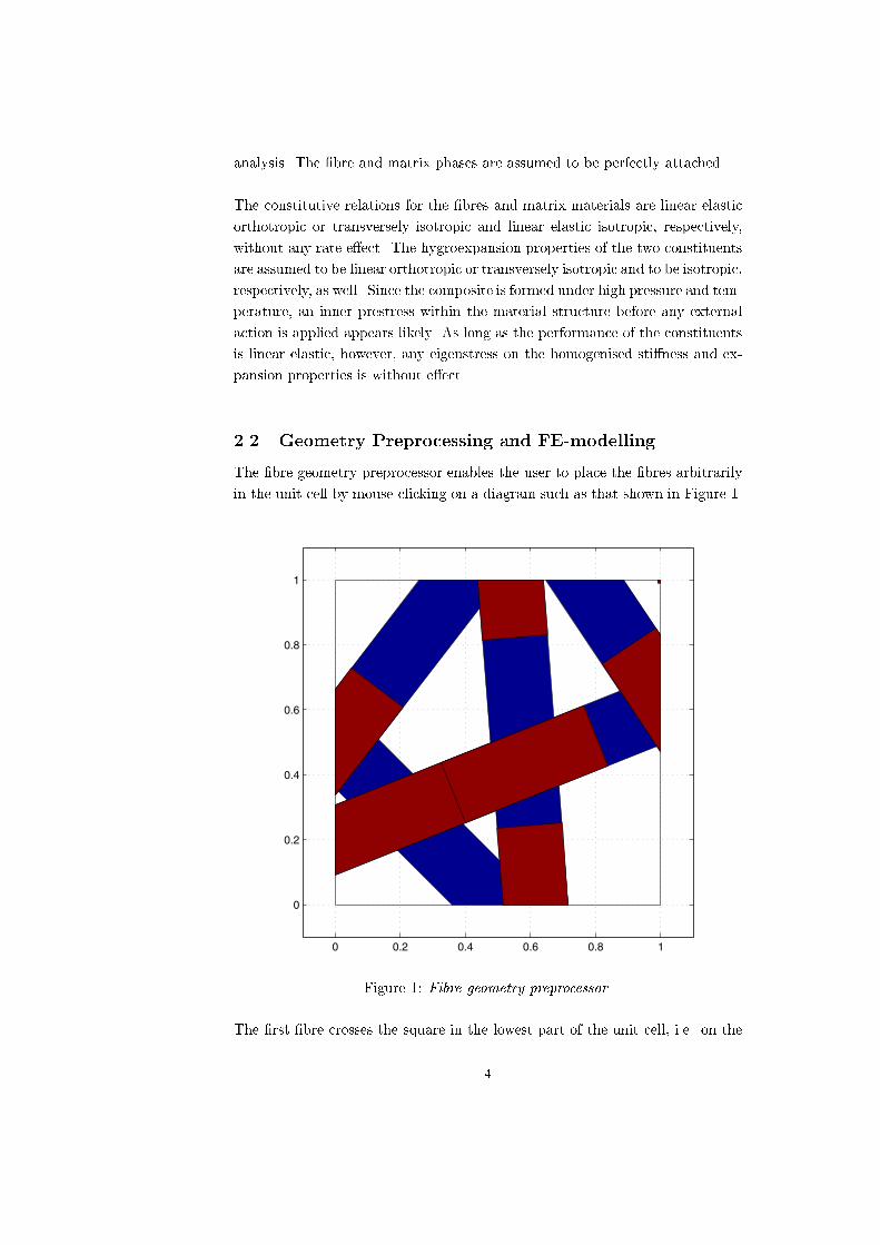
analysis. The �bre and matrix phases are assumed to be perfectly attached.

The constitutive relations for the �bres and matrix materials are linear elastic

orthotropic or transversely isotropic and linear elastic isotropic, respectively,

without any rate e�ect. The hygroexpansion properties of the two constituents

are assumed to be linear orthotropic or transversely isotropic and to be isotropic,

respectively, as well. Since the composite is formed under high pressure and tem-

perature, an inner prestress within the material structure before any external

action is applied appears likely. As long as the performance of the constituents

is linear elastic, however, any eigenstress on the homogenised sti�ness and ex-

pansion properties is without e�ect.

2.2 Geometry Preprocessing and FE-modelling

The �bre geometry preprocessor enables the user to place the �bres arbitrarily

in the unit cell by mouse-clicking on a diagram such as that shown in Figure 1.

0 0.2 0.4 0.6 0.8 1

0

0.2

0.4

0.6

0.8

1

Figure 1: Fibre geometry preprocessor.

The �rst �bre crosses the square in the lowest part of the unit cell, i.e. on the

4

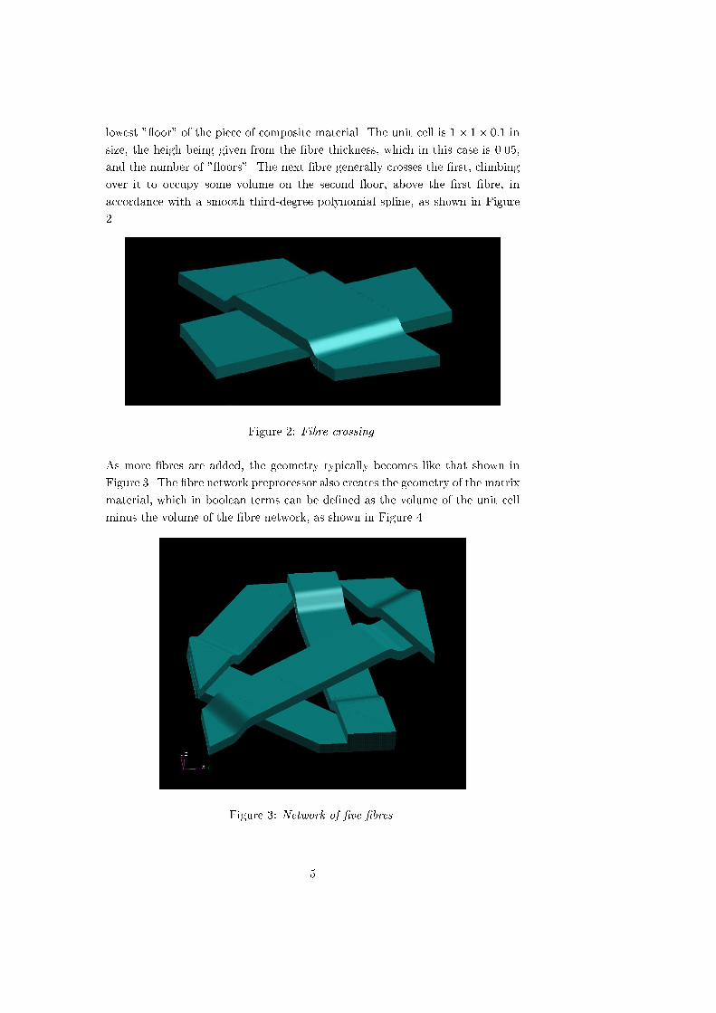
lowest " oor" of the piece of composite material. The unit cell is 1� 1� 0:1 in

size, the heigh being given from the �bre thickness, which in this case is 0.05,

and the number of " oors". The next �bre generally crosses the �rst, climbing

over it to occupy some volume on the second oor, above the �rst �bre, in

accordance with a smooth third-degree polynomial spline, as shown in Figure

2.

Figure 2: Fibre crossing.

As more �bres are added, the geometry typically becomes like that shown in

Figure 3. The �bre network preprocessor also creates the geometry of the matrix

material, which in boolean terms can be de�ned as the volume of the unit cell

minus the volume of the �bre network, as shown in Figure 4.

Figure 3: Network of �ve �bres.

5

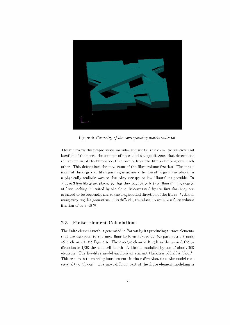
Figure 4: Geometry of the corresponding matrix material.

The indata to the preprocessor includes the width, thickness, orientation and

location of the �bres, the number of �bres and a slope distance that determines

the steepness of the �bre slope that results from the �bres climbing over each

other. This determines the maximum of the �bre volume fraction. The maxi-

mum of the degree of �bre packing is achieved by use of large �bres placed in

a physically realistic way so that they occupy as few " oors" as possible. In

Figure 3 �ve �bres are placed so that they occupy only two " oors". The degree

of �bre packing is limited by the slope distances and by the fact that they are

assumed to be perpendicular to the longitudinal direction of the �bres. Without

using very regular geometries, it is di�cult, therefore, to achieve a �bre volume

fraction of over 40 %.

2.3 Finite Element Calculations

The �nite element mesh is generated in Patran by its producing surface elements

that are extruded to the next oor to form hexagonal, iso-parametric 8-node

solid elements, see Figure 5. The average element length in the x- and the y-

direction is 1/20 the unit cell length. A �bre is modelled by use of about 200

elements. The �ve-�bre model employs an element thickness of half a " oor".

This results in there being four elements in the z-direction, since the model con-

sists of two " oors". The most di�cult part of the �nite element modelling is

6

to make the elements between two " oors" compatible, such that the mesh for

both " oors" is identical. This is achieved by dividing the " oors" into smaller

sections, identical for both " oors". Problems of this sort are based on the fact

that Patran is not an ideal solid modeller. The �nite element model typically

involves about 5000 nodes, which give a system of equations with about 15000

degrees of freedom. These equations are solved in about 20 s, using a single

work station.

Figure 5: Unit cell created from the geometries shown in Figure 3 and 4, with a

�nite element mesh.

3 Material Properties

The matrix material considered in this study is a phenolic resin assumed to be

isotropic, having a Young's modulus of 5.75 Gpa [5] and a Poisson's ratio of

0.3. The hygroexpansion coe�cient, �, is de�ned as the increase in free strain

for a given increase in moisture content, expressed in percent. The unit for �

is [1/%]. A wood �bre is modelled as a transverse isotropic solid having the

material properties shown in Tables 1 and 2. Note that the hygroexpansion

coe�cients in the transverse directions are estimated to be 26 times as great

as those in the longitudinal direction [16]. The adhesion of the constituents is

assumed to be perfect and without any chemical interaction or adsorption.

4 Homogenisation Procedure

Homogenisation is performed by exposing the unit cell to a prescribed defor-

mation in the x-, y- and z-directions, respectively. During the prescribed defor-

mation in the x-direction, the two cell boundaries with a normal vector in the

7

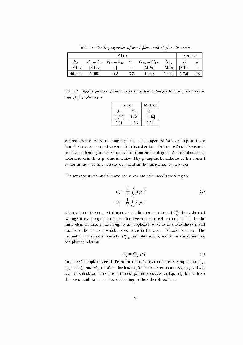
Table 1: Elastic properties of wood �bres and of phenolic resin.

Fibre Matrix

Ex Ey = Ez �xy = �xz �yz Gxy = Gxz Gyz E �

[MPa] [MPa] [-] [-] [MPa] [MPa] [MPa] [-]

40 000 5 000 0.2 0.3 4 000 1 920 5 750 0.3

Table 2: Hygroexpansion properties of wood �bres, longitudinal and transverse,

and of phenolic resin.

Fibre Matrix

�L �T �

[1/%] [1/%] [1/%]

0.01 0.26 0.01

x-direction are forced to remain plane. The tangential forces acting on these

boundaries are set equal to zero. All the other boundaries are free. The condi-

tions when loading in the y- and z-directions are analogous. A prescribed shear

deformation in the x-y-plane is achieved by giving the boundaries with a normal

vector in the y-direction a displacement in the tangential, x-direction.

The average strain and the average stress are calculated according to

"�ij =1

V

ZV

"ijdV (1)

��ij =1

V

ZV

�ijdV

where "�ij are the estimated average strain components and ��ij the estimated

average stress components calculated over the unit cell volume, V [1]. In the

�nite element model the integrals are replaced by sums of the sti�nesses and

strains of the element, which are constant in the case of 8-node elements. The

estimated sti�ness components, D�

ijkl, are obtained by use of the corresponding

compliance relation

"�ij = C�

ijkl��

kl (2)

for an orthotropic material. From the normal strain and stress components "�xx,

"�yy and "�zz and ��xx obtained for loading in the x-direction are Ex, �xy and �xz

easy to calculate. The other sti�ness parameters are analogously found from

the stress and strain results for loading in the other directions.

8

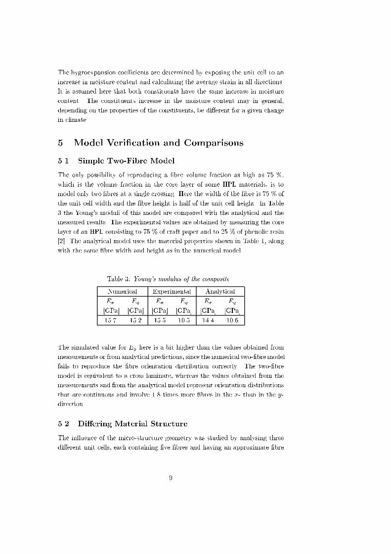
The hygroexpansion coe�cients are determined by exposing the unit cell to an

increase in moisture content and calculating the average strain in all directions.

It is assumed here that both constituents have the same increase in moisture

content. The constituents increase in the moisture content may in general,

depending on the properties of the constituents, be di�erent for a given change

in climate.

5 Model Veri�cation and Comparisons

5.1 Simple Two-Fibre Model

The only possibility of reproducing a �bre volume fraction as high as 75 %,

which is the volume fraction in the core layer of some HPL materials, is to

model only two �bres at a single crossing. Here the width of the �bre is 75 % of

the unit cell width and the �bre height is half of the unit cell height. In Table

3 the Young's moduli of this model are compared with the analytical and the

measured results. The experimental values are obtained by measuring the core

layer of an HPL consisting to 75 % of craft paper and to 25 % of phenolic resin

[2]. The analytical model uses the material properties shown in Table 1, along

with the same �bre width and height as in the numerical model.

Table 3: Young's modulus of the composite.

Numerical Experimental Analytical

Ex Ey Ex Ey Ex Ey

[GPa] [GPa] [GPa] [GPa] [GPa] [GPa]

15.7 15.2 15.5 10.5 14.4 10.6

The simulated value for Ey here is a bit higher than the values obtained from

measurements or from analytical predictions, since the numerical two-�bre model

fails to reproduce the �bre orientation distribution correctly. The two-�bre

model is equivalent to a cross laminate, whereas the values obtained from the

measurements and from the analytical model represent orientation distributions

that are continuous and involve 1.8 times more �bres in the x- than in the y-

direction.

5.2 Di�ering Material Structure

The in uence of the micro-structure geometry was studied by analysing three

di�erent unit cells, each containing �ve �bres and having an approximate �bre

9

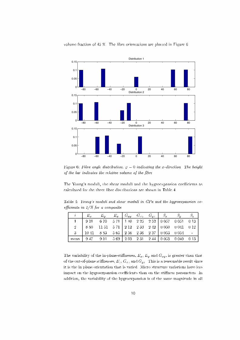
volume fraction of 45 %. The �bre orientations are plotted in Figure 6.

−80 −60 −40 −20 0 20 40 60 800

0.05

0.1

0.15Distribution 1

−80 −60 −40 −20 0 20 40 60 800

0.05

0.1

0.15Distribution 2

−80 −60 −40 −20 0 20 40 60 800

0.05

0.1

0.15Distribution 3

Figure 6: Fibre angle distribution, ' = 0 indicating the x-direction. The height

of the bar indicates the relative volume of the �bre.

The Young's moduli, the shear moduli and the hygroexpansion coe�cients as

calculated for the three �bre distributions are shown in Table 4

Table 4: Young's moduli and shear moduli in GPa and the hygroexpansion co-

e�cients in 1/% for a composite.

i Ex Ey Ex Gxy Gxz Gyz �x �y �z

1 9.21 6.70 5.71 1.40 2.25 2.52 0.057 0.051 0.13

2 8.80 11.51 5.71 2.12 2.33 2.42 0.050 0.041 0.12

3 10.41 8.83 5.65 2.56 2.36 2.37 0.053 0.054 -

mean 9.47 9.01 5.69 2.03 2.31 2.44 0.053 0.049 0.13

The variability of the in-plane-sti�nesses, Ex, Ey and Gxy, is greater than that

of the out-of-plane sti�nesses, Ez, Gxz and Gyz. This is a reasonable result since

it is the in-plane orientation that is varied. Micro-structure variations have less

impact on the hygroexpansion coe�cients than on the sti�ness parameters. In

addition, the variability of the hygroexpansion is of the same magnitude in all

10

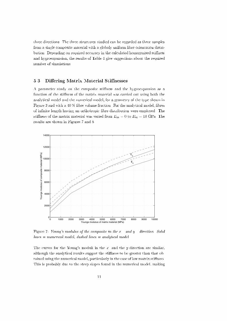
three directions. The three structures studied can be regarded as three samples

from a single composite material with a globaly uniform �bre orientation distri-

bution. Depending on required accuracy in the calculated homogenised sti�ness

and hygroexpansion, the results of Table 4 give suggestions about the required

number of simulations.

5.3 Di�ering Matrix Material Sti�nesses

A parameter study on the composite sti�ness and the hygroexpansion as a

function of the sti�ness of the matrix material was carried out using both the

analytical model and the numerical model, for a geometry of the type shown in

Figure 3 and with a 40 % �bre volume fraction. For the analytical model, �bres

of in�nite length having an orthotropic �bre distribution were employed. The

sti�ness of the matrix material was varied from Em = 0 to Em = 10 GPa. The

results are shown in Figures 7 and 8.

0 1000 2000 3000 4000 5000 6000 7000 8000 9000 100000

2000

4000

6000

8000

10000

12000

14000

Youngs modulus of matrix material (MPa)

You

ngs

mod

ulus

of c

ompo

site

mat

eria

l (M

Pa) E

y

Ex

Figure 7: Young's modulus of the composite in the x� and y� direction. Solid

lines = numerical model, dashed lines = analytical model.

The curves for the Young's moduli in the x- and the y-direction are similar,

although the analytical results suggest the sti�ness to be greater than that ob-

tained using the numerical model, particularly in the case of low matrix sti�ness.

This is probably due to the steep slopes found in the numerical model, making

11

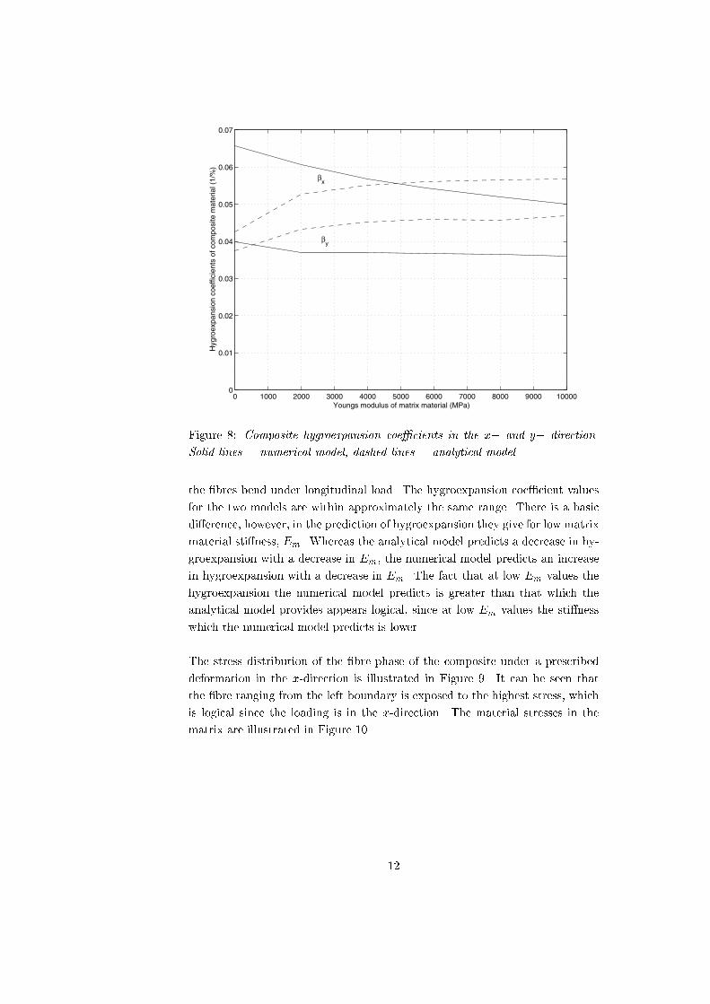
0 1000 2000 3000 4000 5000 6000 7000 8000 9000 100000

0.01

0.02

0.03

0.04

0.05

0.06

0.07

Youngs modulus of matrix material (MPa)

Hyg

roex

pans

ion

coef

ficie

nts

of c

ompo

site

mat

eria

l (1/

%)

βx

βy

Figure 8: Composite hygroexpansion coe�cients in the x� and y� direction.

Solid lines = numerical model, dashed lines = analytical model.

the �bres bend under longitudinal load. The hygroexpansion coe�cient values

for the two models are within approximately the same range. There is a basic

di�erence, however, in the prediction of hygroexpansion they give for low matrix

material sti�ness, Em. Whereas the analytical model predicts a decrease in hy-

groexpansion with a decrease in Em, the numerical model predicts an increase

in hygroexpansion with a decrease in Em. The fact that at low Em values the

hygroexpansion the numerical model predicts is greater than that which the

analytical model provides appears logical, since at low Em values the sti�ness

which the numerical model predicts is lower.

The stress distribution of the �bre phase of the composite under a prescribed

deformation in the x-direction is illustrated in Figure 9. It can be seen that

the �bre ranging from the left boundary is exposed to the highest stress, which

is logical since the loading is in the x-direction. The material stresses in the

matrix are illustrated in Figure 10.

12

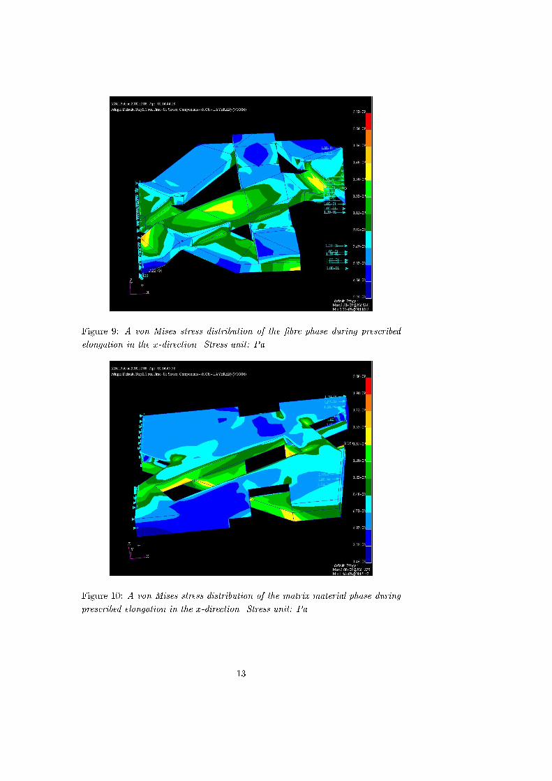
Figure 9: A von Mises stress distribution of the �bre phase during prescribed

elongation in the x-direction. Stress unit: Pa

Figure 10: A von Mises stress distribution of the matrix material phase during

prescribed elongation in the x-direction. Stress unit: Pa

13

6 Concluding Remarks

A 3D �nite element model for the sti�ness and hygroexpansion analysis of �bre

composite materials was presented. The model provides a good representation of

the microstructure of a composite material, such as HLP, and opens up for many

possibilities, such as that of creating models of the complex microstructures of

various composite materials, perhaps simply on the basis of the information

contained in microscopic images. Parameter studies can also be performed of

any parameter. The behaviour of new materials which do not yet exists can

be analysed as well. The model can also be used to simulate network mechan-

ics models, such as of paper, without the use of matrix material. The model

provides reasonably accurate estimates of the sti�ness and hygroexpansion of

a composite through use of a �ve-�bre version of the model and of three nom-

inally equal simulations. The �ve-�bre model may not be su�cient, however,

for simulating �bre networks without matrix materials.

In this study only time-independent properties were investigated. The model is

also intended, however, for future use in studies of time dependent properties

such as creep and mechanosorption which are important for wood and wood

composite materials.

7 Future Work

The model studied here was developed as a tool for the analysis of long �bre

network composites such as HPL, but it can be developed further so as to achieve

an even better representation of the morphology of the composite:

� The �bre packing can be increased to well above the present maximum

of about 45% for a multi-�bre random geometry. This can be done by

making the �bre shape more exible, allowing the �bres to be curved in

the plane, be twisted or be of varying width and thickness.

� Use of larger unit cells containing more �bres is required to obtain a better

representation of a random structure with a continuous �bre orientation

distribution. This will result in lesser variability between nominally equal

simulations and will accordingly require fewer simulations in order for ac-

curate mean value estimates to be made. The use of larger models will

be facilitated by the ongoing development of more e�cient �nite element

software and of faster computers.

14

� The �bre geometry and its internal structure can be more accurately rep-

resented by modelling it as a collapsed pipe in which the inclination of

an orthotropic orientation in the �bre walls is induced by the micro-�bril

angle.

15

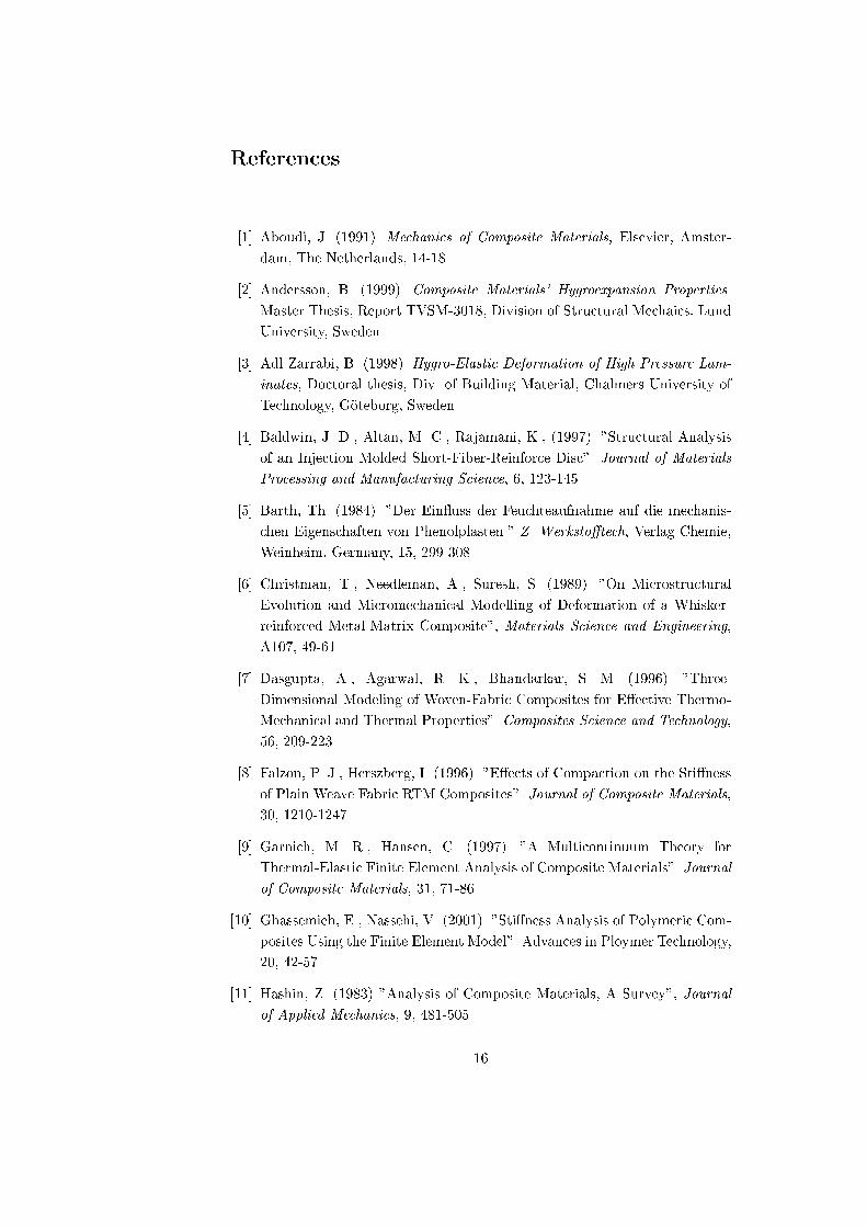
References

[1] Aboudi, J. (1991). Mechanics of Composite Materials, Elsevier, Amster-

dam, The Netherlands, 14-18.

[2] Andersson, B. (1999). Composite Materials' Hygroexpansion Properties.

Master Thesis, Report TVSM-3018, Division of Structural Mechaics, Lund

University, Sweden.

[3] Adl Zarrabi, B. (1998). Hygro-Elastic Deformation of High Pressure Lam-

inates, Doctoral thesis, Div. of Building Material, Chalmers University of

Technology, G�oteborg, Sweden

[4] Baldwin, J. D., Altan, M. C., Rajamani, K., (1997). "Structural Analysis

of an Injection Molded Short-Fiber-Reinforce Disc". Journal of Materials

Processing and Manufacturing Science, 6, 123-145.

[5] Barth, Th. (1984). "Der Ein uss der Feuchteaufnahme auf die mechanis-

chen Eigenschaften von Phenolplasten." Z. Werksto�tech, Verlag Chemie,

Weinheim, Germany, 15, 299-308.

[6] Christman, T., Needleman, A., Suresh, S. (1989). "On Microstructural

Evolution and Micromechanical Modelling of Deformation of a Whisker-

reinforced Metal-Matrix Composite", Materials Science and Engineering,

A107, 49-61.

[7] Dasgupta, A., Agarwal, R. K., Bhandarkar, S. M. (1996). "Three-

Dimensional Modeling of Woven-Fabric Composites for E�ective Thermo-

Mechanical and Thermal Properties". Composites Science and Technology,

56, 209-223.

[8] Falzon, P. J., Herszberg, I. (1996). "E�ects of Compaction on the Sti�ness

of Plain Weave Fabric RTM Composites". Journal of Composite Materials,

30, 1210-1247.

[9] Garnich, M. R., Hansen, C. (1997). "A Multicontinuum Theory for

Thermal-Elastic Finite Element Analysis of Composite Materials". Journal

of Composite Materials, 31, 71-86.

[10] Ghassemieh, E., Nassehi, V. (2001). "Sti�ness Analysis of Polymeric Com-

posites Using the Finite Element Model". Advances in Ploymer Technology,

20, 42-57.

[11] Hashin, Z. (1983) "Analysis of Composite Materials, A Survey", Journal

of Applied Mechanics, 9, 481-505.

16

[12] Heyden, S. (2000). Network modelling for the evaluation of mechanical

properties of cellulose �bre u�., Doctoral thesis, Report TVSM-1011, Div.

of Structural Mechanics, Lund University, Sweden.

[13] Ismar, H., Schroter, F., Streicher, F. (2000). "Modeling and Numerical

Simulation of the Mechanical Behaviour of Woven SiC/SiC regarding a

Three-Dimensional Unit Cell". Computational Materials Science, 19, 320-

328.

[14] Matlab - The language of technical computation. (1998) The Math Works

Inc., Natick, Ma, USA.

[15] Nilsen, N., Niskanen, K. (1996) "A 3D simulation model for paper struc-

ture." Progress in Paper Physics - A Seminar Proceedings.

[16] Persson, K. (2001). Micromechanical modelling of wood and �bre proper-

ties. Doctoral thesis, Division of Structural Mechanics, Lund University,

Sweden.

[17] Stahl, D. C., Cramer, S. M. (1998). "A Three-Dimensional Network Model

for a Low Density Fibrous Composite". Journal of Engineering Materials

and Technology, 120, 126-130.

[18] St�alne, K., Gustafsson, P. J. (2000). "A 3D Model for Analysis of Sti�ness

and Hygroexpansion Properties of Fibre Composite Materials", Journal of

Engineering Mechanics, in press.

[19] Termonia, Y. (1994). "Structure-Property Relationships in Short-Fiber-

Reinforced Composites". Journal of Polymer Science, Part B: Polymer

Physics, 32, 969-979.

[20] Thom, H. (1999). "Finite Element Modeling of Plain Weave Composites"

Journal of Composite Materials, 33, 1491-1510.

[21] Toll, S. (1998). "Packing Mechanics of Fiber Reinforcements". Polymer

Engineering and Science, 38, 1337-1350.

[22] Tucker, C.L., Liang, E. (1999). "Sti�ness Predictions for Unidirectional

Short-Fiber Composites: Review and Evaluation" Composites Science and

Technology 59, 655-671.

[23] Whitcomb, J. D., Chapman, C. D., Tang, X. (2000). "Derivation of Bound-

ary Conditions for Micromechanics Analyses of Plain and Satin Weave

Composites". Journal of Composite Materials, 34, 724-747.

[24] Zeman, J., Sejnoha, M., (2001). "Numerical Evaluation of E�ective Elas-

tic Properties of Graphite Fiber Tow Impregnated by Polymer Matrix".

Journal of the Mechanics and Physics of Solids, 49, 69-90.

17