modelling of wastewater systems - technical … science and technology, 37 ... the thesis is...
TRANSCRIPT

MODELLING
OF
WASTEWATER SYSTEMS
Henrik Bechmann
Lyngby 1999ATV Erhvervsforskerprojekt EF 623
IMM-PHD-1999-69
IMM

ISSN 0909-3192ISBN 87-88306-01-1
c© Copyright 1999 by Henrik BechmannPrinted by jespersen offsetBound by Hans Meyer, Technical University of Denmark

The work documented in this thesis is also published in the following papers:
PaperA: Bechmann, H., Nielsen, M. K., Madsen, H., and Poulsen, N. K. (1998).Control of sewer systems and wastewater treatment plants using pollutantconcentration profiles.Water Science and Technology, 37(12), 87–93.
PaperB: Bechmann, H., Madsen, H., Poulsen, N. K., and Nielsen, M. K. (1999).Grey box modelling of first flush and incoming wastewater at a wastewatertreatment plant.Environmetrics, 11(1), 1–12.
PaperC: Bechmann, H., Nielsen, M. K., Madsen, H., and Poulsen, N. K. (1999).Grey-box modelling of pollutant loads from a sewer system.UrbanWater,1(1), 71–78.
PaperD: Nielsen, M. K., Bechmann, H., and Henze, M. (1999).Modelling andtest of aeration tank settling ATS. In8th IAWQ Conference on Design,Operation and Economics of Large Wastewater Treatment plants, pages199–206. International Association on Water Quality, IAWQ, BudapestUniversity of Technology, Department of Sanitary and Environmental En-gineering.
PaperE: Bechmann, H., Nielsen, M. K., Poulsen, N. K., and Madsen, H. (1999).Grey-box modelling of aeration tank settling. Submitted.
PaperF: Bechmann, H., Nielsen, M. K., Poulsen, N. K., and Madsen, H. (1999).Effects and control of aeration tank settling operation. Submitted.
iii

iv

Preface
This thesis has been prepared at the Department of Mathematical Modelling(IMM), The Technical University of Denmark, and Krüger A/S, in partial ful-filment of the requirements for the degree of Ph.D. in engineering.
The thesis is concerned with the modelling of wastewater processes with theobjective of using the models for control of sewer systems and wastewatertreatment plants. The main contribution to this field includes both linear andnonlinear dynamic stochastic modelling of the influents to wastewater treat-ment plants as well as modelling of processes in the wastewater treatmentplant.
Ramløse, 12th November 1999.
Henrik Bechmann
v

vi

Acknowledgements
I wish to express my gratitude to all who have contributed to this research.
First of all, I wish to thank my supervisors, Professor Henrik Madsen, IMM,DTU, Associate Professor Niels Kjølstad Poulsen, IMM, DTU, and SeniorEngineer Marinus K. Nielsen, Krüger A/S, for guidance, encouragement andconstructive criticism during this work.
I wish to thank my colleagues at Krüger, especially past and present membersof the STAR/S&P group: Tine B. Önnerth, Jacob Carstensen, Steven Isaacs,Kenneth F. Janning, Kenneth Kisbye, Peter Lindstrøm, Thomas Munk-Nielsen,Niels B. Rasmussen, Henrik A. Thomsen, and Dines Thornberg. Thanks arealso due to my colleagues of the Krüger R&D Department: Kjær H. An-dreasen, Claus P. Dahl, René Dupont and Flemming Norsk, as well as to ourmanager Rune Strube. Furthermore, I am very grateful to Lærke Christensenfor proofreading this thesis and making suggestions regarding my use of theEnglish language.
At IMM, I wish to thank past and present members of the Time Series Analy-sis group, the Control group and the Statistics group: Helle Andersen, JudithL. Jacobsen, Harpa Jonsdottir, Trine Kvist, Karina Stender, Sabine Vaillant,Jens Strodl Andersen, Klaus Kaae Andersen, Mikkel Baadsgaard, Alfred K.Joensen, Henrik Aalborg Nielsen, Jan Nygaard Nielsen, Torben Skov Nielsen,Magnus Nørgaard, Payman Sadegh, Uffe Høgsbro Thygesen, and Peter Thyre-god.
vii

viii
Special thanks to Henrik Öjelund for reading a draft of this thesis and goodsuggestions concerning improvements.
Also, I am very grateful to Associate Professor Peter Steen Mikkelsen, De-partment of Environmental Science and Engineering (IMT), DTU, for havingshared his knowledge about urban runoff and urban runoff systems with me.
Thanks are also due to the staff at the wastewater treatment plants of Skive,Aalborg East and Aalborg West, especially Pernille Iversen, for their supportduring data collection, for carrying out laboratory analyses and for running theon-line sensors.
I also thank my former colleague at UNI•C, Peter Busk Laursen, for sharinghis profound knowledge and experience with LATEX and friends, and valuableadvice about preparing the thesis.
This research was funded by the Danish Academy for Technical Sciences andKrüger A/S, to whom I would like to express my gratitude.
Finally, I am grateful to my family, my wife Iben and our three children,Louise, Daniel and Mathilde as well as my parents and parents in law for theirsupport and great patience during the preparation of this thesis.
Summary
In this thesis, models of pollution fluxes in the inlet to 2 Danish wastewatertreatment plants (WWTPs) as well as of suspended solids (SS) concentrationsin the aeration tanks of an alternating WWTP and in the effluent from theaeration tanks are developed. The latter model is furthermore used to analyzeand quantify the effect of the Aeration Tank Settling (ATS) operating mode,which is used during rain events. Furthermore, the model is used to propose acontrol algorithm for the phase lengths during ATS operation.
The models are mainly formulated as state space model in continuous time withdiscrete-time observation equations. The state equations are thus expressed instochastic differential equations. Hereby it is possible to use the maximumlikelihood estimation method to estimate the parameters of the models. A Kal-man filter is used to estimate the one-step ahead predictions that are used in theevaluation of the likelihood function. The proposed models are of the grey-boxtype, where the most important physical relations are combined with stochasticterms to describe the deviations between model and reality as well as measure-ment errors.
The pollution flux models are models of the COD (Chemical Oxygen Demand)flux and SS flux in the inlet to the WWTP. COD is measured by means of a UVabsorption sensor while SS is measured by a turbidity sensor. These modelsinclude a description of the deposit of COD and SS amounts, respectively, inthe sewer system, and the models can thus be used to quantify these amounts aswell as to describe possible first flush effects. The buildup and flush out of thedeposits are modelled by differential equations, thus the models are dynamic
ix
x
models. The dynamic models are furthermore compared to simpler static mo-dels and it is found that the dynamic models are better at modelling the fluxesin terms of the multiple correlation coefficientR2.
The model of the SS concentrations in the aeration tanks of an alternatingWWTP as well as in the effluent from the aeration tanks is a mass balancemodel based on measurements of SS in one aeration tank and in the commonoutlet of all the aeration tanks, respectively. This model is a state space modelwith the SS concentrations and the sludge blanket depths in the aeration tanksas state variables and with the SS concentrations in one aeration tank and inthe common outlet as observations.
The SS concentration model is used to quantify the benefits of ATS operationin terms of increased hydraulic capacity. The model is furthermore used topropose a control algorithm for the phase lengths during ATS operation. Thequantification of the benefits of ATS operation as well as the proposal for acontrol algorithm is based on the assumption that if the SS concentration inthe secondary clarifier increases beyond a plant and situation specific amountabove the normal dry weather level, the SS concentration in the effluent in-creases to an unacceptable level. It was found that ATS increases the hydrauliccapacity of the WWTP considered by more than 167%, while the proposedcontrol algorithm is yet to be implemented in full scale.

Resumé (in Danish)
I denne afhandling er der udviklet modeller for henholdsvis forureningsfluxi indløbet til 2 danske renseanlæg og for koncentrationer af suspenderet stof(SS) i luftningstankene på et alternerende renseanlæg såvel som i udløbet fraluftningstankene. Sidstnævnte model er desuden anvendt til at analysere ogkvantificere effekten af Aeration Tank Settling (ATS) driftsformen, der anven-des under regn. Desuden er modellen anvendt til at foreslå en styringsalgoritmefor faselængderne under ATS drift.
Modellerne er hovedsagligt formuleret som tilstandsmodeller i kontinuert tidmed diskret tids observationsligninger. Tilstandsligningerne er derfor formu-leret i stokastiske differentialligninger. Herved er det muligt at anvende max-imum likelihood estimationsmetoden til at estimere modellernes parametre,idet et Kalmanfilter anvendes til at estimere et-trins prædiktionerne der brugestil evaluering af likelihood-funktionen. De foreslåede modeller er af grey-boxtypen hvor de væsentligste fysiske sammenhænge benyttes i modelformule-ringen kombineret med stokastiske termer til at beskrive afvigelserne mellemmodel og virkelighed samt målefejl.
Forureningsfluxmodellerne er modeller for COD (Chemical Oxygen Demand)flux og SS flux, i indløbet til renseanlægget. COD er målt vha. en UV ab-sorptionssensor mens SS er målt vha. en turbiditetssensor. Disse modellerinkluderer en beskrivelse af aflejringerne af henholdsvis COD og SS mængderi afløbssystemet, hvorved modellerne kan anvendes til at kvantificere dissemængder, samt til at beskrive eventuelle first flush effekter. Opbygningenog udskylningen af aflejringerne er modelleret vha. differentialligninger, så
xi

xii
modellerne er dynamiske modeller. De dynamiske modeller er desuden sam-menlignet med simplere statiske modeller og det er fundet at de dynamiskemodeller er bedre til at modellere fluxene målt vha. den multiple korrelationskoefficientR2.
Modellen for SS koncentrationerne i luftningstankene i et alternerende rensean-læg såvel som i udløbet fra luftningstankene er en massebalancemodel baseretpå målinger af henholdsvis SS i én luftningstank og i det fælles udløb fraalle luftningstankene. Denne model er en tilstandsmodel med SS koncentra-tionerne samt slamspejlsdybderne i luftningstankene som tilstande, og med SSkoncentrationerne i den ene luftningstank samt i det fælles udløb som observa-tioner.
SS koncentrationsmodellen er anvendt til at kvantificere fordelene ved ATSdrift målt i øget hydraulisk kapacitet ved at kvantificere SS mængderne i luft-ningstankene under ATS drift. Modellen er desuden anvendt til at foreslåen styringsalgoritme for faselængderne under ATS drift. Kvantificeringen affordelene ved ATS drift samt den foreslåede styringsalgoritme er baseret påen antagelse om at stiger SS koncentrationen i efterklaringstanken mere enden anlægs- og situationsspecifik størrelse over normal tørvejrsniveau, stiger SSkoncentrationerne i udløbet til et uacceptabelt niveau. Det er fundet at ATSøger den hydrauliske kapacitet for det betragtede renseanlæg med mere end167 %, mens den foreslåede styringsalgoritme endnu ikke er implementeret ifuldskala.
Contents
I Background and discussion 1
1 Introduction 3
1.1 Modelling approaches. . . . . . . . . . . . . . . . . . . . . . 4
1.1.1 Sewer system modelling. . . . . . . . . . . . . . . . 6
1.1.2 Sedimentation and first flush. . . . . . . . . . . . . . 6
1.1.3 Control of sewer systems. . . . . . . . . . . . . . . . 8
1.1.4 Wastewater treatment plant modelling. . . . . . . . . 8
1.1.5 Control of wastewater treatment plants. . . . . . . . 9
1.1.6 Purpose. . . . . . . . . . . . . . . . . . . . . . . . . 10
1.2 Outline of the thesis. . . . . . . . . . . . . . . . . . . . . . . 10
2 Stochastic modelling of dynamic systems 13
2.1 The Wiener process. . . . . . . . . . . . . . . . . . . . . . . 13
xiii

xiv CONTENTS
2.2 Stochastic differential equations. . . . . . . . . . . . . . . . 14
2.3 Stochastic state space models. . . . . . . . . . . . . . . . . . 15
2.4 Maximum likelihood estimation. . . . . . . . . . . . . . . . 16
2.5 The extended Kalman filter. . . . . . . . . . . . . . . . . . . 19
2.6 Uncertain and missing observations. . . . . . . . . . . . . . 21
2.7 Model validation . . . . . . . . . . . . . . . . . . . . . . . . 22
2.7.1 Tests in the model. . . . . . . . . . . . . . . . . . . 22
2.7.2 Graphical methods. . . . . . . . . . . . . . . . . . . 22
2.7.3 Residual analysis. . . . . . . . . . . . . . . . . . . . 23
2.7.4 Cross validation . . . . . . . . . . . . . . . . . . . . 25
2.8 Grey-box modelling. . . . . . . . . . . . . . . . . . . . . . . 26
2.9 Summary . . . . . . . . . . . . . . . . . . . . . . . . . . . . 27
3 Results and discussion 29
3.1 Sewer models. . . . . . . . . . . . . . . . . . . . . . . . . . 30
3.1.1 Cumulated flux vs. cumulated flow. . . . . . . . . . 31
3.1.2 Suggestions concerning future research – sewer models38
3.2 ATS operation. . . . . . . . . . . . . . . . . . . . . . . . . . 38
3.2.1 Suggestions concerning future research– aeration tank SS model. . . . . . . . . . . . . . . . 44
4 Conclusions 47

CONTENTS xv
II Included papers 51
List of Included papers 53
A Control of sewer systems and wastewater treatment plantsusing pollutant concentration profiles.Published inWater Science and Technology,37(12), pp. 87–93, 1998 55
Abstract . . . . . . . . . . . . . . . . . . . . . . . . . . . . . 57
Introduction . . . . . . . . . . . . . . . . . . . . . . . . . . . 57
Data catchment. . . . . . . . . . . . . . . . . . . . . . . . . 58
Theory. . . . . . . . . . . . . . . . . . . . . . . . . . . . . . 59
Results - Discussion. . . . . . . . . . . . . . . . . . . . . . . 62
Conclusions. . . . . . . . . . . . . . . . . . . . . . . . . . . 64
B Grey box modelling of first flush and incoming wastewaterat a wastewater treatment plant.Published inEnvironmetrics,11(1), pp. 1–12, 2000 67
Summary . . . . . . . . . . . . . . . . . . . . . . . . . . . . 69
Introduction . . . . . . . . . . . . . . . . . . . . . . . . . . . 69
The measurement system. . . . . . . . . . . . . . . . . . . . 70
COD and SS. . . . . . . . . . . . . . . . . . . . . . . . . . . 71
A dynamical model of the deposited pollutants. . . . . . . . 71
The parameter estimation method. . . . . . . . . . . . . . . 73

xvi CONTENTS
Results and Discussion. . . . . . . . . . . . . . . . . . . . . 76
Conclusion . . . . . . . . . . . . . . . . . . . . . . . . . . . 81
Acknowledgements. . . . . . . . . . . . . . . . . . . . . . . 82
C Grey-box modelling of pollutant loads from a sewer system.Published inUrbanWater,1(1), pp. 71–78, 1999 83
Abstract . . . . . . . . . . . . . . . . . . . . . . . . . . . . . 85
Key words. . . . . . . . . . . . . . . . . . . . . . . . . . . . 85
Introduction . . . . . . . . . . . . . . . . . . . . . . . . . . . 85
The measurement system. . . . . . . . . . . . . . . . . . . . 86
Models of the pollution concentrations and fluxes. . . . . . . 87
Estimation methods. . . . . . . . . . . . . . . . . . . . . . . 90
Results and discussion. . . . . . . . . . . . . . . . . . . . . 93
Conclusions. . . . . . . . . . . . . . . . . . . . . . . . . . . 97
Acknowledgements. . . . . . . . . . . . . . . . . . . . . . .100
D Modelling and test of Aeration Tank Settling ATS.Published inProceedings of the 8th IAWQ Conference on Design, Opera-tion and Economics of Large Wastewater Treatment Plantspp. 199–206.International Association on Water Quality, IAWQ, Budapest University ofTechnology, Department of Sanitary and Environmental Engineering101
Abstract . . . . . . . . . . . . . . . . . . . . . . . . . . . . .103
Key words. . . . . . . . . . . . . . . . . . . . . . . . . . . .103
CONTENTS xvii
Introduction . . . . . . . . . . . . . . . . . . . . . . . . . . .103
Theory for modelling . . . . . . . . . . . . . . . . . . . . . .105
Physical model . . . . . . . . . . . . . . . . . . . . . . . . .106
Alternating systems. . . . . . . . . . . . . . . . . . . 106
Recirculating plants . . . . . . . . . . . . . . . . . . 108
Plant capacity. . . . . . . . . . . . . . . . . . . . . . . . . .109
Practical test. . . . . . . . . . . . . . . . . . . . . . . . . . .109
Discussion. . . . . . . . . . . . . . . . . . . . . . . . . . . .112
Conclusion . . . . . . . . . . . . . . . . . . . . . . . . . . .113
Acknowledgements. . . . . . . . . . . . . . . . . . . . . . .113
E Grey-box modelling of aeration tank settling.Submitted. 115
Abstract . . . . . . . . . . . . . . . . . . . . . . . . . . . . .117
Key words. . . . . . . . . . . . . . . . . . . . . . . . . . . .117
Introduction . . . . . . . . . . . . . . . . . . . . . . . . . . .117
Dry weather and ATS operation. . . . . . . . . . . . . . . . 118
Theory. . . . . . . . . . . . . . . . . . . . . . . . . . . . . .119
Estimation method . . . . . . . . . . . . . . . . . . . . . . .126
Results and discussion. . . . . . . . . . . . . . . . . . . . . 129
Conclusions. . . . . . . . . . . . . . . . . . . . . . . . . . .136

xviii CONTENTS
Acknowledgements. . . . . . . . . . . . . . . . . . . . . . .136
F Effects and control of Aeration Tank Settling.Submitted. 137
Abstract . . . . . . . . . . . . . . . . . . . . . . . . . . . . .139
Key words. . . . . . . . . . . . . . . . . . . . . . . . . . . .139
Introduction . . . . . . . . . . . . . . . . . . . . . . . . . . .139
Theory. . . . . . . . . . . . . . . . . . . . . . . . . . . . . .143
Dry weather operation. . . . . . . . . . . . . . . . . 145
Choice of operating mode. . . . . . . . . . . . . . . 146
Results and discussion. . . . . . . . . . . . . . . . . . . . . 147
Economic advantages of ATS operation. . . . . . . . 150
Conclusions. . . . . . . . . . . . . . . . . . . . . . . . . . .151
Acknowledgements. . . . . . . . . . . . . . . . . . . . . . .152
Bibliography 153
Ph.D. theses from IMM 163

Part I
Background and discussion
I
1

Chapter 1
Introduction
Urban drainage was introduced to improve sanitary conditions. It involvesthe diversion of wastewater and storm water out of the cities as efficiently aspossible and away from the surface of the streets. However, the discharge ofwastewater has a major impact on the receiving waters. Potentially insufficientor no wastewater treatment could devastate the ecological balance of nature,e.g. by lowered oxygen levels and possibly death of fish in the receiving waters.Hence, wastewater treatment plants has in this century been established andupgraded to remove pollutants in form of organic matter and nutrients fromthe wastewater.
As a consequence of the cholera epidemics in Europe in the middle of the 19thcentury, sewer systems were established, to divert the wastewater out of thecities. Then the wastewater could be removed from the cities, but the pollutionwas just transported to the surrounding environment. The organic pollution inthe wastewater resulted in loss of oxygen in the recipients, which lead to thedevelopment of wastewater treatment plants that remove organic matter. Nutri-ents in form of ammonia, nitrate and phosphate stimulate the growth of algaewhich in the receiving waters and result in excessive loss of oxygen and un-desirable changes in the aquatic life. Hence, nutrient removal was introducedon the wastewater treatment plants. In Denmark, the introduction of nutrientremoval was mainly caused by the water pollution act enacted in 1987. Today,the wastewater treatment is so effective that the critical situations arise during
3

4 CHAPTER 1. INTRODUCTION
rain storms, during which the upper limits of the sewers and wastewater treat-ment plants are reached. This result in untreated wastewater being lead to thereceiving waters. Hence, the focus is today on extension of the sewer systemswith detention basins to store the excessive water from a rain storm until therain stops. Another possibility is to use modern on-line measurement equip-ment combined with on-line controllers to control the sewers and wastewatertreatment plants so that more water can be handled.
To be able to design the optimal control laws the dynamics of the sewers andwastewater treatment plants has to be understood.
The understanding of the dynamic behavior of sewer systems and wastewatertreatment plants is today often formulated as dynamic models. As the modelscan be formulated in many ways, it is important that the model formulationand complexity is in agreement with the modelling objective, i.e. some modelsare developed to yield a very detailed description of the involved processeswhile other models are developed to be operational for prediction and controlpurposes.
1.1 Modelling approaches
Deterministic (white-box) models are developed from the idea that a full un-derstanding of nature can be obtained by identifying and describing all thephysical, chemical and biological laws that govern the system concerned. TheIAWQ1 Activated Sludge Models for the processes in an activated sludge was-tewater treatment plant (Henze et al., 1987, 1995, 1999; Gujer et al., 1999) andthe commercially available urban drainage modelling tools based on the St.Vernant equations (Chow et al., 1988) such as Mouse (Lindberg et al., 1989;Crabtree et al., 1995; Mark et al., 1995, 1998b), are examples of deterministicmodels. The deterministic models are often formulated in continuous time, i.e.the dynamics are described by differential equations. Due to the large numberof parameters it is often impossible to estimate the parameters uniquely fromavailable measurements.
1IAWQ is an abbreviation for International Association on Water Quality, formerly Inter-national Association for Water Pollution Research and Control abbreviated IAWPRC. In 1999International Water Association, IWA, was formed by the merger of IAWQ and InternationalWater Services Association, IWSA.

1.1. MODELLING APPROACHES 5
Black-box models (Ljung, 1995, 1999; Sjöberg et al., 1995) are developed fol-lowing a data based approach. The objective is to describe the input-outputrelations by equations that do not reflect physical, chemical, biological etc.considerations. Time series models: Auto Regressive (AR) models, Auto Re-gressive Moving Average (ARMA), AR with eXternal input (ARX), ARMAwith eXternal input (ARMAX), Box-Jenkins (transfer function) models etc.(Box and Jenkins, 1976; Box et al., 1994; Ljung, 1995, 1999; Madsen, 1995;Poulsen, 1995) are examples of black-box models. These models are formu-lated in discrete time, i.e. the dynamics of the phenomenon concerned aredescribed by difference equations. The time series models include stochasticterms to account for uncertainties in model formulation and measurements. Asthe models do not incorporate any prior knowledge, the parameters have to beestimated. Neural networks are another type of black-box models. The pa-rameters of neural networks are also found by an estimation method, but theterminology is that neural networkslearn by training (see e.g.Sjöberg et al.(1995)).
Grey-box models are based on the most important physical, chemical and bi-ological relations and with stochastic terms to count in uncertainties in modelformulation as well as in observations. The objective is to have physicallyinterpretable parameters that are possible to estimate by means of statisticalmethods. Grey-box models are often formulated as a combination of contin-uous time and discrete time relations. The physical relations are formulatedin continuous time, with differential equations to describe the dynamics, andthe observation equations are expressed as discrete time relations, as measure-ments are taken at discrete time events. By including stochastic terms in boththe continuous time description of the system and the discrete time descriptionof the observations, it is possible to distinguish between modelling uncertain-ties and measurement uncertainties, and to quantify the uncertainties.
Physical insight can also be used to establish models formulated in discretetime only (Young and Wallis, 1985; Young et al., 1997). However, the esti-mated parameters are not directly the parameters of the underlying continuoustime model, even though there are unique relations between the discrete timeand continuous time parameters.
6 CHAPTER 1. INTRODUCTION
1.1.1 Sewer system modelling
Sewer systems are often modelled by means of commercially available soft-ware like the Storm Water Management Model, SWMM (Meinholz et al.,1974), Hydroworks (Heip et al., 1997) and Mouse (Lindberg et al., 1989; Crab-tree et al., 1995; Mark et al., 1995, 1998b). Modelling with such packages hasbeen used as a planning tool for introducing real time control of sewer systems(Entem et al., 1998; Hernebring et al., 1998; Mark et al., 1998a), where themodelling software is used to simulate the sewers.
The time series modelling approach has been used byCapodaglio(1994) tomake one day ahead predictions of the water flow in a sewer system basedon measurements of rainfall.Delleur and Gyasi-Agyei(1994) use transferfunction models to predict suspended solids concentrations in sewers from ob-servations of temperature and flow rate. Modelling of flow rate from rainfallobservations has been carried out byRuan and Wiggers(1997).
Liong and Chan(1993) use neural networks to predict storm runoff volumesfrom a catchment. The predicted volumes from the neural networks are com-pared with output from the SWMM model.Nouh (1996) applies neural net-works to model the peak concentrations of total suspended solids, nitratesand total phosphorus in sewer flows, and compares the results with those ofSWMM.
The grey-box method is applied byGrum(1998) to model suspended organicmatter (suspended COD concentration) and the water level at an overflowstructure in a Dutch combined sewer system.
1.1.2 Sedimentation and first flush
Sedimentation in combined sewers (sewers that handle both municipal waste-water and runoff water) and the first flush phenomenon are closely related tothe different flow conditions during dry weather and wet weather. If sedimen-tation of pollutants in the sewer (and on impervious areas of the catchment)can occur during dry weather periods, the sediments can be flushed out of thesewer during wet weather situations, due to the increased flow. In the first partof the rain event the concentrations will be increased, thus the term first flush.

1.1. MODELLING APPROACHES 7
If the rain continues after the sewer is cleaned, the rain water is assumed todilute the municipal wastewater, with lower concentrations as a result.
Ashley and Crabtree(1992) analyse the sources of sediments in sewers, howthe sediments can be classified and how they are deposited in combined sew-ers. The flushing effects are treated byGeiger(1987); Deletic (1998); Sagetet al. (1996); Bertrand-Krajewski et al.(1998); Gupta and Saul(1996), whoclassify the effects by plotting the cumulative load of pollutants (suspendedsolids, COD etc.) normalized with the total amount of pollutants against thecumulative flow normalized with the total amount of water for a storm event,see Fig.1.1. If the observed curve is above the equilibrium liney = x, flushing
Cumulative flow
Cum
ulat
ive
pollu
tant
load
0 20 40 60 80 100%0
%
20
40
60
80
100
Dilutio
n
Flushin
g
Equili
brium
Figure 1.1. Cumulative pollution curves.
is taking place and if the observed curve is below the equilibrium line dilutionhas occurred. It should be noted that this method treats all storm events equal,and it is not possible from an observed curve to see if the origin was a lightrain event or a heavy thunder storm.

8 CHAPTER 1. INTRODUCTION
Gupta and Saul(1996) perform regression analyses on the cumulative loadof pollutants and find that peak rainfall intensity, the storm duration and theantecedent dry weather period are most informative among the analysed vari-ables.
1.1.3 Control of sewer systems
The introduction of automatic control of sewer systems is a cost effective wayto improve the effluent quality, compared e.g. to building new overflow struc-tures, as automatic control is expected to enable better utilization of the existingfacilities.
By means of appropriate models, predictive control algorithms can be estab-lished. These algorithms utilize predictions from the models to select the bestcontrol action at a given time.
Entem et al.(1998), Hernebring et al.(1998), andMark et al.(1998b) preparefor the application of the Mouse model for on-line control purposes, i.e. acomplicated deterministic model, suitable for simulation studies, is expectedto produce predictions applicable for on-line control, even thoughCarstensenet al. (1996) stress that no single model exists that is suitable for both plan-ning, detailed analysis and on-line control.Carstensen and Harremoës(1997)compared the flow predictions from a Mouse model used on-line with a muchsimpler transfer-function model based on measurements of rainfall intensityand time of day only and estimated on observations from the catchment con-sidered, and finds that the transfer-function model is much better in predictingthe flow. It is thus not expected that white-box models like Mouse is usable foron-line purposes.
1.1.4 Wastewater treatment plant modelling
Activated sludge wastewater treatment plants are often modelled by the IAWQActivated Sludge Models (Henze et al., 1987, 1995, 1999; Gujer et al., 1999).Commercial software that implements the models is available, see e.g.EFORVersion 3.0(1998). Computer models based on the IAWQ models are usedto simulate different control strategies and the possible benefits (Dupont and
1.1. MODELLING APPROACHES 9
Sinkjær, 1994; Rangla et al., 1998).
Novotny et al.(1991); Capodaglio et al.(1992); Berthouex and Box(1996) ap-ply the traditional time series analysis models to wastewater treatment plants.Novotny et al.(1991) andCapodaglio et al.(1992) use physical insight in formof mass balances combined with Euler approximation to establish correspond-ing discrete time models.
Ward et al.(1996) combine the Activated Sludge Model No. 1 (Henze et al.,1987) with time series models to establish a hybrid model of the activatedsludge process and to enable prediction of suspended solids in the effluent.
Zhao et al.(1999) compare the Activated Sludge Model No. 2 (Henze et al.,1995) with a simplified model and a neural net model, whilePu and Hung(1995) establish a neural network model for a trickling filter plant.
Modelling of secondary clarifiers is treated inEkama et al.(1997), which in-clude a description of the Vesilind model (Vesilind, 1968, 1979) for hinderedsludge settling velocity.Härtel and Pöpel(1992) have re-parameterized theoriginal Vesilind mode, to include the dependency of sludge volume index,SVI, on the settling velocity.Dupont and Dahl(1995) suggest a model that isadequate for both free and hindered settling.
Comparison of different one-dimensional sedimentation models is carried outby Grijspeerdt et al.(1995) and Koehne et al.(1995). In Grijspeerdt et al.(1995) both steady state and dynamic properties of the examined models arecompared. It is found that the Takács model (Takács et al., 1991) is the mostreliable. Koehne et al.(1995) conclude that the models considered all modelstorm water flow situations well, but lack sufficient accuracy in simulating dryweather situations.
1.1.5 Control of wastewater treatment plants
Concepts of control of wastewater treatment plants are treated byOlsson et al.(1989) andOlsson(1992), who also treat the instrumentation problem as wellas the subject of building models suitable for control purposes. Note that themodel structures suggested are of the time series analysis type, and not of thedetailed deterministic IAWQ activated sludge model type.

10 CHAPTER 1. INTRODUCTION
Results from the introduction of on-line instrumentation combined with ad-vanced control strategies in wastewater treatment plants are reported byNielsenand Önnerth(1995) andÖnnerth and Bechmann(1995), where both more costeffective operation and better treatment results are obtained.
1.1.6 Purpose
The purpose of this research project is to establish on-line operational modelsfor the wastewater coming to a wastewater treatment plant and for selected pro-cesses in the plant, and to suggest control algorithms that utilize the existingfacilities in the sewer and treatment plant in an optimal way. The project is acontribution towards the total integrated control of sewer systems and waste-water treatment plants.
1.2 Outline of the thesis
This thesis is based on 6 papers written during the project and is divided intotwo parts. The first part contains a summary of the theory behind the modellingcarried out in preparation of the papers as well as a compilation of the resultsof the papers, which are are included in PartII .
In Chapter2 the background for stochastic modelling of dynamic systems isgiven. The aim is to give the background for establishing models comprised ofcontinuous time descriptions of the system dynamics and discrete time descrip-tions of the measurement process. Hence, the chapter begins with a descriptionof stochastic systems. Then a maximum likelihood method for estimation ofthe parameters in the models is presented. This estimation method requires useof the extended Kalman filter, which is introduced next. A method for treatinguncertain and missing observations is presented before the validation of theestimated models is treated. Finally in this chapter, the grey-box modellingconcept is explained and the advantages of this concept is explained.
Chapter3 summarizes the results presented in the papers and discusses aspectsof the work behind the papers not treated in them. The papers should be read inconnection with Chapter3, as the results in the papers are not repeated in this

1.2. OUTLINE OF THE THESIS 11
chapter. Furthermore, suggestions concerning future work in the areas treatedis given.
Finally, the conclusions is presented in Chapter4, after which the papers areincluded.

12 CHAPTER 1. INTRODUCTION
Chapter 2
Stochastic modelling ofdynamic systems
In this chapter some of the mathematical and statistical background for sto-chastic modelling of dynamic systems is given. The objective is to establishthe basis for building continuous time stochastic state space models with dis-crete time observations, to estimate the parameters of the models, and finallyto validate the models.
2.1 The Wiener process
The Scottish botanist Robert Brown observed the irregular motion of pollengrains suspended in water in 1828. The motion, called Brownian motion, waslater explained by the random collisions between the pollen grains and thewater molecules. The Wiener process is a fundamental stochastic process pro-viding a mathematical description of the Brownian motion. The application ofthe Wiener process goes far beyond the study of microscopic suspended par-ticles, and includes modelling of noise and random perturbations in physicalsystems, e.g. thermal noise in electrical circuits.
13

14 CHAPTER 2. STOCHASTIC MODELLING OF DYNAMIC SYSTEMS
The properties that define then-dimensional Wiener process{wt, t ≥ 0} are:
1. w0 = 0 with probability 1
2. The incrementswt1−wt0 ,wt2−wt1 , . . . ,wtk −wtk−1, of the process
are mutually independent for any partitioning of the time interval0 ≤t0 < t1 < · · · < tk <∞
3. The incrementwt − ws for any0 ≤ s < t is Gaussian with mean andcovariance:
E[wt −ws] = 0 (2.1)
V[wt −ws] = Σw(t− s) (2.2)
whereΣw is a positive semi definite matrix.
WhenΣw is the identity matrix, a standard Wiener process is obtained.
Among other important properties of the Wiener process, it should be notedthat the sample paths are continuous with probability one, but nowhere differ-entiable with probability one.
Even though the Wiener process is not differentiable, the formal time derivativeof wt is called Gaussian white noise. This derivative only makes sense as ageneralized function. The process has a uniform spectral density function forall real frequencies, which is a characteristic of white light, hence, the termwhite noise.
See e.g.Melgaard(1994); Madsen and Holst(1996); Øksendal(1995); Jazwin-ski (1970) for more details about the Wiener process.
2.2 Stochastic differential equations
In order to be able to handle stochastic terms in differential equations it isnecessary to introduce stochastic integrals.
Consider the one-dimensional stochastic differential equation:
dXt = f(Xt, t)dt+G(Xt, t)dwt (2.3)
2.3. STOCHASTIC STATE SPACE MODELS 15
wheref(Xt, t) is the drift coefficient,G(Xt, t) is the diffusion coefficient andwt is a standard one-dimensional Wiener process.
A formal integration of (2.3) yields:
Xt = X0 +∫ t
0f(Xs, s)ds+
∫ t
0G(Xs, s)dws (2.4)
The first of the integrals can be interpreted as a standard Riemann integral, butthe second integral is more difficult to handle, as the sample paths of the Wienerprocess have unbound variation (Madsen and Holst, 1996). One solution is toapply the Itô stochastic integral, defined as the mean-square limit of the lefthand rectangular approximation:
N−1∑i=0
G(Xti , ti)(wti+1 − wti) (2.5)
for all partitions0 = t0 < t1 < · · · < tN = t as the maximum step sizemaxi
(ti+1 − ti)→ 0.
More details can be found in e.g.Øksendal(1995); Kloeden and Platen(1995);Madsen et al.(1998); Madsen and Holst(1996).
2.3 Stochastic state space models
State space models are often used to describe dynamic systems. With the in-troduction of stochastic differential equations it is possible to establish contin-uous time stochastic state space models with discrete time observations. Thisis reasonable because physical systems are of a continuous time nature, andmeasurements are taken at discrete time instances. In a stochastic state spacemodel, stochastic terms are used both in the differential equations and in theobservation equations. Hereby, it is possible to distinguish between modellinguncertainty in the differential equations and measurement uncertainty in theobservation equations.
The dynamics of a general non-linear stochastic state space model are de-scribed by:
dXt = f(Xt,U t,θ, t)dt+G(U t,θ, t)dwt, t ≥ 0 (2.6)

16 CHAPTER 2. STOCHASTIC MODELLING OF DYNAMIC SYSTEMS
Here,Xt is the state vector,f is a vector function that describes the evolu-tion of the system as a function of the current state, the input vectorU t, theparameters of the model represented by the parameter vectorθ, and the timet. The vector functionG describes how the noise enters the system. The noiseis represented by the stochastic processw(t), which is ann-th order standardWiener process.
The measurements are taken at discrete time intervals and are thus expressedin the observation equation:
Y k = h(Xk,Uk,θ, tk) + ek, tk ∈ {t0, t1, . . . , tN} (2.7)
whereh is a function that expresses how the measurements are related to thestates and the input, and finallyN is the number of observations. The observa-tion noisee is assumed to be a Gaussian white noise sequence independent ofw. Here, the subscriptk is introduced as a shorthand notation fortk.
2.4 Maximum likelihood estimation
When a stochastic state space model of a given system is formulated and mea-surements from the system are obtained, the parameters are to be estimated.Even though different approaches to the estimation problem are described inthe literature (see e.g.Ljung (1999)), only the maximum likelihood methodwill be described here.
The observations are considered as realizations of stochastic variables. Theobjective of the method is to maximize the probability of the observations, i.e.when a maximum likelihood estimate of the parametersθ is found, no otherparameters will result in a higher probability of the observed data.
In the following it is assumed that the system is observed at regular time in-tervals (i.e. with a constant sampling time). To simplify the notation the timeis normalized with the sampling time, and thus the time index belongs to theset0, 1, 2, . . . , N , whereN is the number of observations. In general everyobservation is a vector.
LetY(t) denote the matrix of all observed outputs until and including timet:
Y(t) = [Y t,Y t−1, . . . ,Y 1,Y 0]′ (2.8)
2.4. MAXIMUM LIKELIHOOD ESTIMATION 17
The unconditional likelihood functionL′(θ;Y(N)) is the joint probability ofall the observations assuming that the parameters are known, i.e.:
L′(θ;Y(N)) = p(Y(N)|θ) (2.9)
In order to express the likelihood function as a product of conditional densities,successive applications of the ruleP (A ∩B) = P (A|B)P (B) are used:
L′(θ;Y(N)) = p(Y(N)|θ)= p(Y N |Y(N − 1),θ)p(Y(N − 1)|θ)
=( N∏t=1
p(Y t|Y(t− 1),θ))p(Y 0|θ)
(2.10)
The conditional likelihood function (conditioned onY 0) is then:
L(θ;Y(N)) =N∏t=1
p(Y t|Y(t− 1),θ) (2.11)
As the increments ofw and the observation noisee are Gaussian, the condi-tional densities for a linear system are also Gaussian. For a non-linear sys-tem like (2.6) we shall assume that the conditional densities are approximatelyGaussian. The Gaussian assumption enables an evaluation of the likelihoodfunction. The normal distribution is completely characterized by the mean andthe covariance. Hence, in order to parameterize the conditional distributions,the conditional mean and conditional covariance are introduced as:
Y t|t−1 = E[Y t|Y(t− 1),θ] and (2.12)
Rt|t−1 = V[Y t|Y(t− 1),θ] (2.13)
respectively. Notice that (2.12) is the one-step prediction and (2.13) the asso-ciated covariance.
The innovations or one-step prediction errors are:
εt = Y t − Y t|t−1 (2.14)
18 CHAPTER 2. STOCHASTIC MODELLING OF DYNAMIC SYSTEMS
Then the conditional likelihood function (2.11) becomes:
L(θ;Y(N))
=N∏t=1
((2π)−m/2 detR−1/2
t|t−1 exp(−12ε′tR−1t|t−1εt)
) (2.15)
wherem is the dimension of theY vector. Traditionally the logarithm of theconditional likelihood function is considered, i.e.
logL(θ;Y(N))
= −12
N∑t=1
(log detRt|t−1 + ε′tR
−1t|t−1εt
)+ const
(2.16)
The maximum likelihood estimate ofθ is found as the value that maximizesthe conditional likelihood functionL(θ;Y(N)), which is the same value thatmaximizeslogL(θ;Y(N)) and minimizes− logL(θ;Y(N)). Thus, the max-imum likelihood estimate ofθ is found as:
θ = arg minDM
N∑t=1
(log detRt|t−1 + ε′tR
−1t|t−1εt
)(2.17)
whereDM is the set of allowed values ofθ
As it is not possible to optimize the likelihood function analytically, a numeri-cal method has to be used. The quasi Newton method is a reasonable choice.
The maximum likelihood estimator is asymptotically normally distributed withmeanθ and variance
D = H−1 (2.18)
whereH is the Hessian given by
{hlk} = −E[ ∂2
∂θl∂θklogL(θ;Y(N))
](2.19)
where{hlk} denotes the element in rowl and columnk of H andθj denoteselementj of θ (Conradsen, 1984a).
An estimate ofD is obtained by equating the observed value with its expecta-tion and applying
{hlk} ≈ −( ∂2
∂θl∂θklogL(θ;Y(N))
)∣∣∣θ=θ
(2.20)

2.5. THE EXTENDED K ALMAN FILTER 19
Equation (2.20) is used to estimate the variance of the parameter estimates.The variance estimate of each of the parameter estimates serves as basis forcalculating t-test values for test under the hypothesis that the parameter is equalto zero. Furthermore, the correlation between the parameter estimates is foundbased on the estimate ofD.
2.5 The extended Kalman filter
The Kalman filter provides estimates of the states in a state space model basedon measurements from the real system. In the maximum likelihood estimationmethod described above, the one step predictions and associated covariancesare needed for calculating the likelihood function, and this is what the Kalmanfilter provides. The Kalman filter is derived for linear systems, and is thusnot directly applicable to non-linear systems. However, the extended Kalmanfilter, based on linearizations of the system equation (2.6) around the currentstate estimate, can then be applied.
Consider now the model described by:
dXt = f(Xt,U t,θ, t)dt+G(θ, t)dwt, (2.21)
with wt being a standard Wiener process. Note thatG is now limited to be afunction of the parameters and time only. The observations are taken at discretetime instantstk and described by:
Y k = h(Xk,Uk,θ, tk) + ek, tk ∈ {t0, t1, . . . , tN} (2.22)
wheree is a Gaussian white noise process independent ofw, and with
ek ∈ N(0,S(θ, tk)) (2.23)
For the continuous-discrete time extended Kalman filter for the state space

20 CHAPTER 2. STOCHASTIC MODELLING OF DYNAMIC SYSTEMS
model (2.21)–(2.22) the prediction equations are:
dXt|k
dt= f(Xt|k,U t,θ, t), t ∈ [tk, tk+1[ (2.24)
dP t|k
dt= A(Xt|k,U t,θ, t)P t|k
+ P t|kA′(Xt|k,U t,θ, t)
+G(θ, t)G′(θ, t), t ∈ [tk, tk+1[
(2.25)
whereA is obtained by a linearization of the system equation (2.21):
A(Xt|k,U t,θ, t) =∂f
∂X
∣∣∣X=Xt|k
(2.26)
At the observation timestk the updates are:
Kk = P k|k−1C′k[CkP k|k−1C
′k + S(θ, tk)]−1 (2.27)
Xk|k = Xk|k−1 +Kk(Y k − h(Xk|k−1,Uk,θ, tk)) (2.28)
P k|k = P k|k−1 −KkCkP k|k−1 (2.29)
whereC is the linearization of the observation equation (2.22):
Ck = C(Xk|k−1,Uk,θ, tk) =∂h
∂X
∣∣∣X=Xk|k−1
(2.30)
To make the integration of (2.24) and (2.25) computationally feasible and nu-merically stable for stiff systems, the time interval[tk, tk+1[ between to subse-quent observations is divided intons subintervals (sub-sampled) and the equa-tions (2.24) and (2.25) are linearized around the state estimate at each sub-sampling time. The state propagation equation for the subinterval[tj , tj+1[becomes:
dXt
dt= f(Xj ,U j ,θ, tj) +A(Xj ,U j ,θ, tj)(Xt − Xj)
= A(Xj ,U j ,θ, tj)Xt
+ (f(Xj ,U j ,θ, tj)−A(Xj ,U j ,θ, tj)Xj) t ∈ [tj , tj+1[
(2.31)
Equation (2.31) has the solution:
Xj+1 = Xj + (Φs(j)− I)(A(Xj ,U j ,θ, tj)−1f(Xj ,U j ,θ, tj)) (2.32)

2.6. UNCERTAIN AND MISSING OBSERVATIONS 21
where
Φs(j) = eA(Xj ,Uj ,θ,tj)τs (2.33)
andτs = tj+1 − tj = T/ns whereT is the sampling time. The matrix ex-ponential can be calculated by e.g. Padé approximation (cf.Madsen et al.(1998)). The state covariance equation becomes:
P j+1 = Φs(j)P jΦs(j)′ + Λs(j) (2.34)
where
Λs(j) =∫ τs
0Φs(j)G(θ, t)G(θ, t)′Φs(j)′ds (2.35)
The extended Kalman filter and the iterated extended Kalman filter are treatedin more detail in e.g.Madsen et al.(1998) andJazwinski(1970).
2.6 Uncertain and missing observations
When working with real systems in an imperfect real world, measurementsare sometimes missing. Sometimes all measurements are available, but themodeller has a priori information that some measurements are less valid thanothers. This is easily handled by adjusting the covarianceS(θ, t) of the ob-servation noise process according to the validity of the measurements. If ameasurement is considered uncertain, the corresponding parameter inS(θ, t)is increased. How much, depends on how uncertain the measurement is. If ameasurement is completely missing, the corresponding variance is ideally setat∞. When increasingS(θ, t) the Kalman gainKk is reduced and the dataupdate (2.28) of the state estimates that depend on the given measurement isreduced correspondingly.
Missing observations in the input data should be handled otherwise. If a singleor at least few observations in a row are missing, these can be substituted byinterpolated values, but in case of long periods with missing observations in-terpolation is often not an option. In this case a change in the model should beconsidered. Sometimes it is possible to change an input variable to an outputvariable, by a slight modification of the model. When this is done, the missingobservations can be handled by means of the method proposed above.
22 CHAPTER 2. STOCHASTIC MODELLING OF DYNAMIC SYSTEMS
2.7 Model validation
When an estimation of the parameters of a model has been carried out, it isimportant to check if the resulting model is satisfactory. This is done by modelvalidation. This is often carried out by applying several methods simultane-ously, of which some will be mentioned in the following.
2.7.1 Tests in the model
The maximum likelihood estimation method provides estimates of the varianceof the parameters, cf. Section2.4, and enables test for the significance of theparameters, i.e. to test whether the parameters are significantly different fromzero. The hypothesis to test is:
H0 : θj = 0 against H1 : θj 6= 0 (2.36)
The test value isθjσjj , whereθj denotes thej-th parameter estimate andσ2jj the
associated variance estimate. As the parameter estimates are asymptoticallynormally distributed, the test value is t distributed, and then a t-test of thehypothesis in (2.36) can be performed (Conradsen, 1984b).
Based on the estimate of the parameter covariance (2.18), the correspondingcorrelation matrix can be computed. Over-parameterization of the model isindicated by closely correlated parameters, i.e. by correlation coefficients be-tween two parameters close to1 or−1. Hence if correlation coefficients closeto 1 or−1 are observed, a reformulation of the model should be considered.
2.7.2 Graphical methods
An obvious method for model validation is a graphical comparison of the mo-del output and the observations, which is simply carried out by plotting theobserved and modelled data. The question is if the outputs of the model seemto match the observations. Note that it is possible to obtain both one-step (ork-step) predictions and simulations from a state space model. The one-steppredictions use the observations at timet and the model equations to predict

2.7. MODEL VALIDATION 23
the observations at the next sample time, while thek-step predictions use theobservations at timet and the model equations to predict the observationsksample times ahead. Simulations are characterized by only using the initialconditions, the inputs and the model to simulate the outputs.
The model output can also be compared with the observations by plotting theresiduals, i.e. the difference between the observations and modelled data. Nat-urally, this can be done for both the one-step (ork-step) predictions and thesimulations.
The states of the model are often interpretable in a physical sense. Hence, thestate estimates should be plotted so that it can be checked if they are realis-tic. This is particularly important, when unmeasured states are included in themodel.
Often the graphical methods reveal possibilities for model enhancements, e.g.inclusion of bounds on states etc.
2.7.3 Residual analysis
The residuals are that part of the observations that the model does not countin. Hence, an analysis of the residuals can provide useful information on howto improve the model, or to improve the confidence in the model. If the mo-del describes the true system well, the residuals are white noise, and it is thusobvious to test if the residuals can in fact be considered as white noise. Further-more, the maximum likelihood method is based on a white noise assumption.If this assumption is not fulfilled, the appealing properties of the method arelost. If the residuals are not white noise, the properties of the residuals cangive an indication of how to improve the model. For instance, if the autocorre-lation function of the residuals show first order autoregressive behaviour, thenan extra state is needed in the model.
24 CHAPTER 2. STOCHASTIC MODELLING OF DYNAMIC SYSTEMS
Auto- and cross-correlations
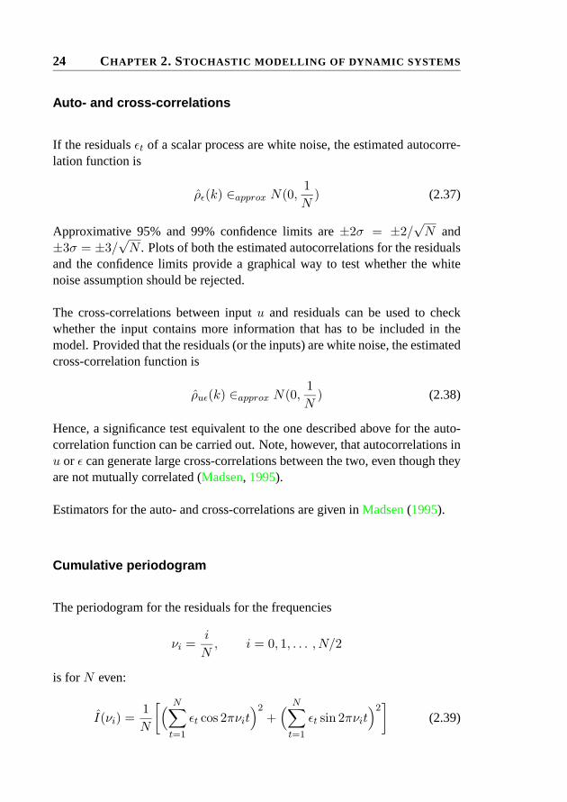
If the residualsεt of a scalar process are white noise, the estimated autocorre-lation function is
ρε(k) ∈approx N(0,1N
) (2.37)
Approximative 95% and 99% confidence limits are±2σ = ±2/√N and
±3σ = ±3/√N . Plots of both the estimated autocorrelations for the residuals
and the confidence limits provide a graphical way to test whether the whitenoise assumption should be rejected.
The cross-correlations between inputu and residuals can be used to checkwhether the input contains more information that has to be included in themodel. Provided that the residuals (or the inputs) are white noise, the estimatedcross-correlation function is
ρuε(k) ∈approx N(0,1N
) (2.38)
Hence, a significance test equivalent to the one described above for the auto-correlation function can be carried out. Note, however, that autocorrelations inu or ε can generate large cross-correlations between the two, even though theyare not mutually correlated (Madsen, 1995).
Estimators for the auto- and cross-correlations are given inMadsen(1995).
Cumulative periodogram
The periodogram for the residuals for the frequencies
νi =i
N, i = 0, 1, . . . , N/2
is forN even:
I(νi) =1N
[( N∑t=1
εt cos 2πνit)2
+( N∑t=1
εt sin 2πνit)2]
(2.39)
2.7. MODEL VALIDATION 25
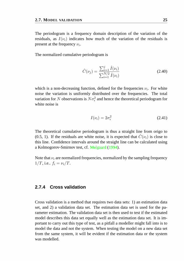
The periodogram is a frequency domain description of the variation of theresiduals, asI(νi) indicates how much of the variation of the residuals ispresent at the frequencyνi.
The normalized cumulative periodogram is
C(νj) =∑j
i=1 I(νi)∑N/2i=1 I(νi)
(2.40)
which is a non-decreasing function, defined for the frequenciesνi. For whitenoise the variation is uniformly distributed over the frequencies. The totalvariation forN observations isNσ2
ε and hence the theoretical periodogram forwhite noise is
I(νi) = 2σ2ε (2.41)
The theoretical cumulative periodogram is thus a straight line from origo to(0.5, 1). If the residuals are white noise, it is expected thatC(νi) is close tothis line. Confidence intervals around the straight line can be calculated usinga Kolmogorov-Smirnov test, cf.Melgaard(1994).
Note thatνi are normalized frequencies, normalized by the sampling frequency1/T , i.e..fi = νi/T .
2.7.4 Cross validation
Cross validation is a method that requires two data sets: 1) an estimation dataset, and 2) a validation data set. The estimation data set is used for the pa-rameter estimation. The validation data set is then used to test if the estimatedmodel describes this data set equally well as the estimation data set. It is im-portant to carry out this type of test, as a pitfall a modeller might fall into is tomodel the data and not the system. When testing the model on a new data setfrom the same system, it will be evident if the estimation data or the systemwas modelled.
26 CHAPTER 2. STOCHASTIC MODELLING OF DYNAMIC SYSTEMS
2.8 Grey-box modelling
Traditionally modelling of dynamic systems has been carried out following oneof two approaches. Theblack-boxconcept is a data based concept, where priorknowledge of the system is not included in the model. Examples of black-boxmodels are the traditional time series models: autoregressive (AR) models,moving average (MA) models, and combinations of these (ARMA). To thesemodels external input can be included to build e.g. ARX or ARMAX models.Another type of black-box models is neural networks. A deterministic modelpurely based on known relations for a system is characterized as awhite-boxmodel. White-box models of complex systems as sewer systems and waste-water treatment plants are often comprised of numerous detailed equations forthe subsystems of the system. White-box models are subject to uncertainties,but a description of these is usually not included in the models, and hence notquantified.
In the environmental sciences, the IAWQ Activated Sludge Models (Henzeet al., 1987, 1995, 1999; Gujer et al., 1999) for the processes in activated sludgewastewater treatment plants, and the Mouse models (Lindberg et al., 1989;Crabtree et al., 1995; Mark et al., 1995, 1998b), based on the St. Vernantequations (Chow et al., 1988) for sewer systems, are examples of deterministicor white-box models.
Often the deterministic models are very detailed and have many parameters,which makes it difficult or impossible to estimate the parameters by ordinarystatistical methods.
The grey-box method is supposed to be the best mix of the two methods. Agrey-box model combines the available knowledge of the most important phys-ical relations with statistical modelling tools. Hereby it is possible to establishmodels with few parameters compared to the white-box models, and with pa-rameters that have physical meaning as opposed to the black-box models. Fur-thermore, the uncertainties are included in the grey-box model, and the param-eters of the noise processes are also estimated. Hence, the model uncertaintiesare quantified.
2.9. SUMMARY 27
2.9 Summary
In this chapter an overview of stochastic modelling is given. The Wiener pro-cess is introduced in order to describe continuous time white noise. Itô stocha-stic integrals and differential equations serve as basis for establishing contin-uous time stochastic state space models. The parameters in such models aresuggested estimated by the maximum likelihood method. The extended Kal-man filter is described, as it calculates the one-step predictions that are neededby the estimation method. When a model is established and the parametersare estimated, it should be validated. Therefore a set of validation tools is pre-sented. Finally, the grey-box modelling approach is presented and comparedwith other modelling approaches.

28 CHAPTER 2. STOCHASTIC MODELLING OF DYNAMIC SYSTEMS

Chapter 3
Results and discussion
The results of the work carried out in the present Ph.D. project are documentedin the papers included in PartII of this thesis. The purpose of this chapter isto discuss aspects of the work that are not treated in the papers, to look at theresults in a broader perspective and to compile the results of the papers, as wellas to suggest areas for future research.
The work presented here is divided into two parts:
The first part focuses on the wastewater coming into the wastewater treatmentplant. The emphasis has been on developing dynamic grey-box models capableof describing the first flush phenomenon by modelling the incoming fluxes,but the results presented also cover the on-line measurements of pollutants andcomparison with static models. This work is presented in PapersA–C.
In the second part, focus is on the biological part of the wastewater treatmentplant, especially during wet weather conditions, where Aeration Tank Settling(ATS) operation is activated. In PaperD a model for ATS is presented and theresult of implementing the model on-line is documented. The model of PaperD forms the basis for further modelling as carried out in preparation of PaperE.
In PaperE ATS operation is described in more detail, and a dynamic grey-
29
30 CHAPTER 3. RESULTS AND DISCUSSION
box model of the suspended solids concentrations in the aeration tanks as wellas in the effluent from these is established. This model is used in PaperFto quantify the advantages of ATS operation in terms of increased hydrauliccapacity of the biological part of the plant and the results are compared with thehydraulic capacity during ordinary dry weather operation. A control algorithmfor enabling ATS and for selecting the optimal combination of phase lengthsduring ATS is also proposed in PaperF.
3.1 Sewer models
The influent pollutant fluxes at two wastewater treatment plants, and hence twocatchments, have been modelled. Skive wastewater treatment plant delivereddata used in the preparation of PaperA and PaperB, and data from AalborgEast wastewater treatment plant was used in PaperC.
The models estimated in PaperA and PaperB are based on the same modelstructure: A diurnal profile of the incoming flux combined with a first orderlinear differential equation for the deposits in the sewer and on imperviousareas of the catchment.
The estimations in PaperA were carried out using the Matlab System Identi-fication Toolbox (Ljung, 1995) with thebj (Box-Jenkins) function in discretetime, and the results were translated to continuous time (with thed2cm func-tion). In this paper the model structure is applied directly to the UV absorptionflux and the turbidity flux. If COD and UV absorption as well as SS and tur-bidity are proportional, this approach is equivalent to modelling COD and SSfluxes, but as the relationships are affine, the models of UV absorption and tur-bidity fluxes are not equivalent to the models of COD and SS fluxes. Howeverin this paper UV absorption and turbidity are thought of as measures of CODand SS concentrations, respectively.
The estimated models are cross validated, i.e. one data set is used for theestimation and another data set is used for the validation of the model. Fur-thermore, the estimated diurnal profiles for UV absorption and turbidity fluxesare shown. The modelled amounts of UV absorption and turbidity deposited inthe sewers are also shown. As it is not possible to estimate the actual levels ofthe deposits in the sewer with the model structure used, only deviations from

3.1. SEWER MODELS 31
the initial level can be found.
In PaperB the COD and SS fluxes are modelled. The estimations were madewith the CTLSM software (Madsen and Melgaard, 1991; Melgaard and Mad-sen, 1991), hence, the parameters are estimated by a maximum likelihoodmethod directly in continuous time. In this paper the standard deviations ofthe parameter estimates are also included.
The modelling carried out in PaperB is based on the same data as used in Pa-perA and the estimated models are cross validated like in PaperA. However,the models of PaperB are models of the COD and SS fluxes (as opposed to themodels of PaperA). In PaperB the estimated amounts of deposits in the sewerare shown as deviations from the unknown average for the time period con-cerned. Due to the fact that the models are of COD and SS fluxes, respectively,the deposits are amounts COD and SS.
In PaperC four different model structures are estimated and compared. Thedata used in this paper are from Aalborg East wastewater treatment plant. Thecontribution from this paper is twofold: 1) The dynamic model structure usedin the previous papers is compared with simpler static models, and 2) Thedynamic model structure is applied to a different sewer system.
Cross validations of the estimated models was not carried out in PaperC. Thiswould, however, be relevant to do so that the different models could be com-pared on a validation data set also.
3.1.1 Cumulated flux vs. cumulated flow
When dealing with sewer systems and rain storms, it is of interest whether firstflushes are present or not. As the proposed models do not directly describewhether and when a first flush is present, this issue will be discussed here.The graph of the normalized cumulated flux vs. cumulated flow is used inthe characterization whether a first flush was present, i.e. a graph with theparametric description:
(x, y) = (
∫ tt0Qdt∫ t1
t0Qdt
,
∫ tt0QXdt∫ t1
t0QXdt
) t0 ≤ t ≤ t1 (3.1)

32 CHAPTER 3. RESULTS AND DISCUSSION
whereX is the concentration of the pollutant concerned,Q is the flow, andt0andt1 denote the start and end times of the rain incident.
When using this method, it is not possible from a given graph to distinguishbetween different types of rain incidents, e.g. between a short intensive thun-derstorm and a long rain with lower intensity.
It is easier to distinguish different rain incidents from the non-normalizedgraph:
(x, y) = (∫ t
t0
Qdt,
∫ t
t0
QXdt) t0 ≤ t ≤ t1 (3.2)
Model 1 of PaperC consists only of a diurnal profile (a harmonic function witha 24-hour period), and is therefore not applicable to storm situations. Model 2models the pollutant fluxes as affine with the flowQX = c0 + c1Q, i.e. thepollutant flux is modelled as a constant level with addition of a term propor-tional to the flow. Hence, the deviation from the constant pollutant flux levelis modelled as a flux with constant concentration. Models 1 and 2 are thus notcapable of describing first flush phenomena. Hence, it is only meaningful toapply the cumulated flow – cumulated flux methodology to models 3 and 4 ofPaperC.
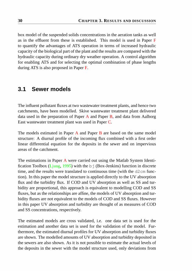
The cumulated flow – cumulated flux methodology is applied to a rain incidentin the data series from Aalborg East wastewater treatment plant. The flow tothe plant during the period in question is shown in Figure3.1
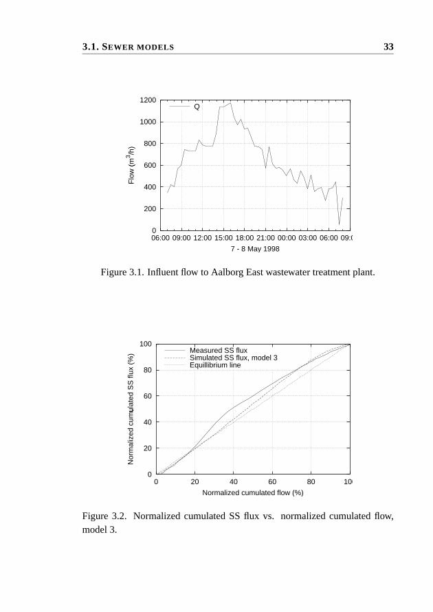
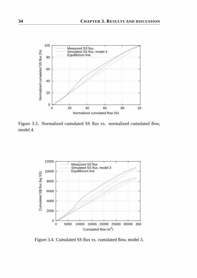
In Figures3.2 and3.3 the normalized cumulated SS flux vs. normalized cu-mulated flow of models 3 and 4 are shown, and in Figures3.4and3.5, the cor-responding non-normalized graphs are shown. Note that the observed fluxesare compared to simulations from the models, and not one (ork) step aheadpredictions. From Figures3.2and3.3 it can be seen that both models can pre-dict increased pollutant concentrations during the rain incident, but also thatthe simulated fluxes are too low in the first approx. 70 – 80 % of the incident.When inspecting the non-normalized graphs in Figures3.4and3.5, it becomesclear that the modelled fluxes are too low as the graphs for the measurementsand the simulations does not end in the same point.
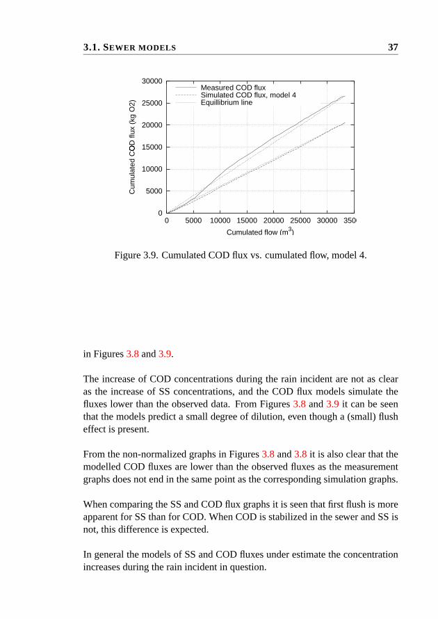
The normalized cumulated COD flux vs. the normalized cumulated flow isshown in Figures3.6 and3.7 with the corresponding non-normalized graphs
3.1. SEWER MODELS 33
0
200
400
600
800
1000
1200
06:00 09:00 12:00 15:00 18:00 21:00 00:00 03:00 06:00 09:00
Flo
w (
m�
3 /h)
7 - 8 May 1998
Q
Figure 3.1. Influent flow to Aalborg East wastewater treatment plant.
0
20
40
60
80
100
0 20 40 60 80 100
Nor
mal
ized
cum
ulat
ed S
S fl
ux (
%)
�
Normalized cumulated flow (%)
Measured SS fluxSimulated SS flux, model 3Equillibrium line
Figure 3.2. Normalized cumulated SS flux vs. normalized cumulated flow,model 3.
34 CHAPTER 3. RESULTS AND DISCUSSION
0
20
40
60
80
100
0 20 40 60 80 100
Nor
mal
ized
cum
ulat
ed S
S fl
ux (
%)
�
Normalized cumulated flow (%)
Measured SS fluxSimulated SS flux, model 4Equillibrium line
Figure 3.3. Normalized cumulated SS flux vs. normalized cumulated flow,model 4.
0
2000
4000
6000
8000
10000
12000
0 5000 10000 15000 20000 25000 30000 35000
Cum
ulat
ed S
S fl
ux (
kg S
S)
�
Cumulated flow (m3)
Measured SS fluxSimulated SS flux, model 3Equillibrium line
Figure 3.4. Cumulated SS flux vs. cumulated flow, model 3.

3.1. SEWER MODELS 35
0
2000
4000
6000
8000
10000
12000
0 5000 10000 15000 20000 25000 30000 35000
Cum
ulat
ed S
S fl
ux (
kg S
S)
�
Cumulated flow (m3)
Measured SS fluxSimulated SS flux, model 4Equillibrium line
Figure 3.5. Cumulated SS flux vs. cumulated flow, model 4.
0
20
40
60
80
100
0 20 40 60 80 100
Nor
mal
ized
cum
ulat
ed C
OD
flux
(%
)
�
Normalized cumulated flow (%)
Measured COD fluxSimulated COD flux, model 3Equillibrium line
Figure 3.6. Normalized cumulated COD flux vs. normalized cumulated flow,model 3.

36 CHAPTER 3. RESULTS AND DISCUSSION
0
20
40
60
80
100
0 20 40 60 80 100
Nor
mal
ized
cum
ulat
ed C
OD
flux
(%
)
�
Normalized cumulated flow (%)
Measured COD fluxSimulated COD flux, model 4Equillibrium line
Figure 3.7. Normalized cumulated COD flux vs. normalized cumulated flow,model 4.
0
5000
10000
15000
20000
25000
30000
0 5000 10000 15000 20000 25000 30000 35000
Cum
ulat
ed C
OD
flux
(kg
O2)
�
Cumulated flow (m3)
Measured COD fluxSimulated COD flux, model 3Equillibrium line
Figure 3.8. Cumulated COD flux vs. cumulated flow, model 3.
3.1. SEWER MODELS 37
0
5000
10000
15000
20000
25000
30000
0 5000 10000 15000 20000 25000 30000 35000
Cum
ulat
ed C
OD
flux
(kg
O2)
�
Cumulated flow (m3)
Measured COD fluxSimulated COD flux, model 4Equillibrium line
Figure 3.9. Cumulated COD flux vs. cumulated flow, model 4.
in Figures3.8and3.9.
The increase of COD concentrations during the rain incident are not as clearas the increase of SS concentrations, and the COD flux models simulate thefluxes lower than the observed data. From Figures3.8 and3.9 it can be seenthat the models predict a small degree of dilution, even though a (small) flusheffect is present.
From the non-normalized graphs in Figures3.8and3.8 it is also clear that themodelled COD fluxes are lower than the observed fluxes as the measurementgraphs does not end in the same point as the corresponding simulation graphs.
When comparing the SS and COD flux graphs it is seen that first flush is moreapparent for SS than for COD. When COD is stabilized in the sewer and SS isnot, this difference is expected.
In general the models of SS and COD fluxes under estimate the concentrationincreases during the rain incident in question.

38 CHAPTER 3. RESULTS AND DISCUSSION
3.1.2 Suggestions concerning future research – sewer mo-dels
As the proposed models are quite simple linear models, it is not surprising thatthey do not describe the observed data perfectly, and that the models should bereformulated, for example by increasing the order of the differential equationdescribing the pollution deposits and/or including non-linear terms. Further-more, the sub-model for buildup and flush-out of pollutants in the sewer can besplit up into two: 1) A sub-model describing the buildup of pollutants in dryweather periods, and 2) A sub-model for flush-out during wet weather peri-ods. These two sub-models need not be of the same order – the buildup modelcould for example be made up of a first order differential equation, whereas theflush-out model could be of a higher order. The switch between the two sub-models should be controlled by the flow, and implemented by application ofsmooth threshold functions (see PaperE for an application of smooth thresholdfunctions).
As first flushes and dilutions are expected to be a result of limited amounts ofpollutants deposited in the sewer, introduction of limitations on the depositsin the sewer system could be an important extension to the dynamic model4. However, to be able to estimate the limits of the deposits, the data mustinclude periods where the limits are reached, i.e. intensive rain events wherethe sewer system is cleaned and long dry weather periods where the depositedpollutants reach the upper limits. Such data series with a sufficient number ofobservations of the extreme events might be difficult to obtain.
3.2 ATS operation
Aeration Tank Settling (ATS) is introduced to enable the biological treatmentfacilities to handle larger wastewater flows than possible with ordinary dryweather operation. The traditional way to handle storm situations is to store theexcess water that the biological part of the plant cannot handle in storm tanks,if available. If the plant is not equipped with storm tanks or if they are alreadyfull, the excess water has to bypass the aeration tanks and secondary clarifiers.Hence, bypass wastewater, which has not been biologically treated, is beinglead to the receiving waters. The details of ATS operation are described in
3.2. ATS OPERATION 39
PapersD–F.
When ATS is activated, the biological tanks of the plant are capable of handlinga significantly larger flow, and thus to remove nutrients from considerably morewastewater during a rain event.
PaperD documents the first preliminary modelling of ATS operation. Themodel is formulated in discrete time, and forms the basis for the work of thefollowing papers.
In PaperE the modelling of suspended solids in the aeration tanks of an al-ternating BioDenipho plant as well as in the effluent from the aeration tanksduring ATS is documented. In this paper the model is formulated in contin-uous time with discrete-time observations. The modelling is based on mea-surements of flow to the biological partQi , the recirculation flowQr, theconcentrations of suspended solids in one aeration tankXssm6, in the recir-culation flowXssr and in the effluent from the aeration tanksXssoutat. Theflow path through each of the aeration tank pairs as well as the mixing sig-nals (fpkl, mk andml for the aeration tank pair consisting of aeration tanksk and l, (k, l) ∈ {(1, 2), (3, 4), (5, 6)}, are also used as inputs to the model.The incoming flowQi is actually measured in the effluent from the secondaryclarifier, but when the water dynamics of the aeration tanks and clarifier areinsignificant, these flows are equal.
In Figure 3.10 the data set used for the parameter estimation in PaperE isshown. The flow path and mixing signals are only shown for aeration tanks 5and 6, as the signals for the other two tank pairs are delayed versions of thesedata. The data set covers two ATS operation events with a dry weather periodin between. The first ATS event covers the period from 25 October 1:30 toOctober 26 15:50. Then the plant is in dry weather operation until October 2712:30. The second ATS period continues to the end of the data set on October29 0:00.
Note that the average SS concentration in the influent to the aeration tanks(assuming that the SS concentration inQin is zero) calculated as
Xssinat(t) =Qr
Qi +QrXssr (3.3)
is included in the graphs. It is reasonable to assume that the SS concentrationin Qin is zero as the estimations carried out in preparation of PaperE showed

40 CHAPTER 3. RESULTS AND DISCUSSION
0
2
4
6
8
10
12
1000
m3 /h
Aalborg W. WWTP
QinQr
02468
1012141618
g/m
� 3
Aalborg W. WWTP
XssrQr*Xssr/(Qi+Qr)
0
2
4
6
8
10
g/m
� 3
Aalborg W. WWTP
Xssm6Xssoutat
0 1
0 1
0 1
25 Oct00:00
25 Oct12:00
26 Oct00:00
26 Oct12:00
27 Oct00:00
27 Oct12:00
28 Oct00:00
28 Oct12:00
29 Oct00:00
Aalborg W. WWTP
fp56m5m6
Figure 3.10. The data set used for the parameter estimation.

3.2. ATS OPERATION 41
that this concentration was insignificant.
In Figures3.11and3.12estimated and simulated SS concentrations and sludgeblanket depths for a part of the estimation data set used in PaperE are shown.Both the estimated and the simulated variables are output from the extendedKalman filter. The estimated values are the data updated state estimates, wherethe measurements have been used to compute the results. The simulated dataare the results of a simulation of the model, i.e. only the input data to the model(flow path through the aeration tanks, mixing signals, return sludge concentra-tions, inflow and return sludge flow) and initial values of the SS concentrationsand sludge blanket depths in the aeration tanks are used. The flow pathfp56
through the considered aeration tank pair is also included. Whenfp56 = 1the incoming wastewater as well as the return sludge flow is directed to aera-tion tank 5 and the clarifier is fed from aeration tank 6 and vice versa whenfp56 = 0.
From Figure3.11it can be seen that the sludge concentration is increasing inthe aeration tank with discharge to the clarifier and decreasing in the influenttank. When comparing the SS concentrations in the aeration tanks in Figure3.11with the average SS concentration in the wastewater entering the aerationtanks in Figure3.10, it is noted that the average SS concentration in the in-fluent is about 3 g SS/m3 and that the SS concentrations in the aeration tanksfluctuate around 4.5 g SS/m3. Hence, the SS concentration in the wastewaterentering the influent aeration tank is lower than in the wastewater already in thetank. As the amount of water in the tanks is almost constant, the fluctuations inthe sludge concentrations in the aeration tanks are caused by the fact that theincoming water pushes the sludge over to the effluent tank, and when the flowpath is changed the sludge is pushed back again. The result of the sludge mov-ing between the aeration tanks is seen in the SS concentrations in the effluentfrom the tanks. When the flow path is switched, the effluent is taken from atank with a lower concentration. The concentration in the effluent tank thenincreases until the next change of flow path, but as sludge settling occurs in thetank, the SS concentration in the effluent is not increasing at the same rate asin the aeration tank.
The estimated and simulated sludge blanket depths in aeration tanks 5 and6 are shown in Figure3.12. It can be seen that the sludge blanket depth islimited to about 0.8 m. Unfortunately, the aeration tanks at the Aalborg Westplant are not equipped with sludge blanket sensors, so it is not possible to

42 CHAPTER 3. RESULTS AND DISCUSSION
2
2.5
3
3.5
4
4.5
5
5.5
6
25 Oct ’9800:00
25 Oct ’9812:00
26 Oct ’9800:00
26 Oct ’9812:00
27 Oct ’9800:00
27 Oct ’9812:00
28 Oct ’9800:00
28 Oct ’9812:00
29 Oct ’9800:00
1
0
g/l
Flo
w p
ath
Aalborg W. WWTP, e22e-8-2
Estimated Xss5(t|t)Estimated Xss6(t|t)
fp,56
2
2.5
3
3.5
4
4.5
5
5.5
6
25 Oct ’9800:00
25 Oct ’9812:00
26 Oct ’9800:00
26 Oct ’9812:00
27 Oct ’9800:00
27 Oct ’9812:00
28 Oct ’9800:00
28 Oct ’9812:00
29 Oct ’9800:00
1
0
g/l
Flo
w p
ath
Aalborg W. WWTP, e22e-8-2
Simulated Xss5(t|t0)Simulated Xss6(t|t0)
fp,56
Figure 3.11. Estimated and simulated SS concentrations in aeration tanks 5and 6.
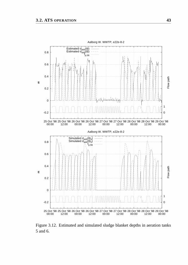
3.2. ATS OPERATION 43
-0.2
0
0.2
0.4
0.6
0.8
25 Oct ’9800:00
25 Oct ’9812:00
26 Oct ’9800:00
26 Oct ’9812:00
27 Oct ’9800:00
27 Oct ’9812:00
28 Oct ’9800:00
28 Oct ’9812:00
29 Oct ’9800:00
1
0
m
�
Flo
w p
ath
Aalborg W. WWTP, e22e-8-2
Estimated dsb5(t|t)Estimated dsb6(t|t)
fp,56
-0.2
0
0.2
0.4
0.6
0.8
25 Oct ’9800:00
25 Oct ’9812:00
26 Oct ’9800:00
26 Oct ’9812:00
27 Oct ’9800:00
27 Oct ’9812:00
28 Oct ’9800:00
28 Oct ’9812:00
29 Oct ’9800:00
1
0
m
�
Flo
w p
ath
Aalborg W. WWTP, e22e-8-2
Simulated dsb5(t|t0)Simulated dsb6(t|t0)
fp,56
Figure 3.12. Estimated and simulated sludge blanket depths in aeration tanks5 and 6.

44 CHAPTER 3. RESULTS AND DISCUSSION
compare the estimated and simulated values with measurements. However, it isstraight forward to include sludge blanket measurements in the model, if sludgeblanket sensors are installed. From the estimated sludge blanket depths it isseen that they become negative, especially in dry weather periods. This is ofcourse not feasible, but this physical limitation was not included in the model.However, the negative values occurring are small, and thus not considered amajor problem.
The estimated model is used in PaperF to simulate different operating modesof the plant, i.e. dry weather operation and 5 different ATS strategies, whichresult in different flow capacity increases at the plant. The simulations areused to quantify how much ATS operation can increase the flow capacity, aswell as to propose a control algorithm for selecting the optimal ATS operatingmode. Examples of both dry weather and ATS operation situations at AalborgWest wastewater plant are included in PaperF to illustrate a real ATS operationsituation and to compare with a dry weather situation. It should be noted thatthe ATS event illustrated is controlled by another control algorithm than theone proposed in the paper. In order to make the comparison fair and becausethe load of the plant varies over the week, both situations include a Saturdayand a Sunday. The selection of the days was carried out by first looking for astorm situation and then selecting a similar period with dry weather.
3.2.1 Suggestions concerning future research– aeration tank SS model
In the model for SS in the aeration tanks as well as in the effluent from theseestablished in PaperF, parameters for errors in the measurements ofXssr andXssoutat are estimated simultaneously with the other model parameters. Ofcourse there can also be systematic errors in the flow measurements, but param-eters for errors in the flow observations were not estimated. Error parametersfor the flow observations should be included in the model to make it possibleto test whether there are significant errors in the measurements of the flows.
The model includes all 6 aeration tanks of Aalborg West wastewater treatmentplant, which are operated in an identical way except for time delays betweeneach of the tank pairs. The time delay is equal to the re-sampling interval (12minutes). The benefits of using a full 6-tank model compared to a simplified

3.2. ATS OPERATION 45
2-tank model are expected to be of minor significance, as the 6-tank modelis made up of 3 identical 2-tank models, with a time delay of 1 re-samplinginterval between each of the tank pairs. A simplified model should thereforebe tried and the results compared with the full 6-tank model. The advantageof a simplified model is that it will only contain 4 states (2 SS concentrationsand 2 sludge blanket depths) instead of the 12 states (6 SS concentrations andsludge blanket depths) of the full model, and hence the computations requiredfor estimation and simulation are reduced significantly. Furthermore will theapplication of the model on other plants with a different number of aerationtanks be simpler.
As can be seen from the estimated sludge blanket depths in Figure3.12, thedepths sometimes become negative. As this is not physically possible, thesludge blanket sub-model could therefore be reformulated to prevent negativesludge blanket depths values, e.g. by means of a logarithm transformation ofthe sludge blanket depth equations.
The sludge blanket depths are unobserved states of the model. It is thus notpossible to compare the modelled sludge blanket depths with measurements.Therefore addition of sludge blanket depth sensors in at least on of the aera-tion tanks could be used to gain more confidence in the model. Furthermorewill addition of sludge blanket sensors enable estimation of the sludge settlingparameters.
The possibilities for developing a better model ofXssoutatshould be investi-gated as the current model does not perform as well as desired. It is expectedthat a goodXssoutatmodel is required for modelling the SS conditions in thesecondary clarifier and in the effluent from here. Better modelling ofXssoutat
could be achieved by refining the sludge settling model, e.g. by introducingmore layers in the sludge settling model than the two used here.
Control of ATS operation
The content of suspended solids in the secondary clarifier has not been mod-elled in the present work. Inclusion of a clarifier model is another extensionoption, which should enable predictions of the SS concentrations in the effluentto the receiving waters, and thus make it possible to design control algorithmsthat can control the effluent SS concentrations to the recipient closer to the

46 CHAPTER 3. RESULTS AND DISCUSSION
allowed limits and thus further optimize ATS operation.
Finally, a combined ATS control strategy based on both information from theinfluent to the wastewater treatment plant and from the current state in the ae-ration tanks and secondary clarifier should be established. The control strategyshould control both the ATS operation and the bypass flow. Hereby, it shouldbe possible to decide whether it is advantageous to use the ATS capabilities tohandle the incoming flow or some of the flow should bypass the biological partof the plant. The use of available detention basins at the treatment plant shouldbe included in the strategy as well. The control of ATS, bypass flow and de-tention basins at the wastewater treatment plant should be integrated with thecontrol of the overflow structures, storage basins, pumping stations etc., of thesewer system to enable optimal operation of the total system.
Chapter 4
Conclusions
In this thesis, stochastic models for the incoming wastewater to two differentwastewater treatment plants as well as for the SS concentrations in the aerationtanks of an alternating wastewater treatment plant and in the effluent from theaeration tanks are presented. The latter model is furthermore used to quantifythe effects of the Aeration Tank Settling (ATS) operating mode as well as topropose a control algorithm for controlling the phase lengths during ATS.
The objective of modelling the incoming wastewater to a wastewater treatmentplant was to model possible first flush effects. In PapersA andB dynamicmodels of the COD flux and SS flux in the influent to two Danish wastewatertreatment plants are developed. The models include the buildup and flush outof pollutants in the form of COD and SS in the sewer and on impervious areasof the catchment. The results show that the models can be used to describesome of the first flush effect, but also that the models in some situations predicta dilution even though this is not the case. It is furthermore found that themodels make it possible to estimate the deviations in COD and SS deposits inthe sewer and on impervious areas of the catchment from an initial level butnot the actual amounts in the sewer.
In PaperC the dynamic models are compared to simpler static models to quan-tify the improvements of including the dynamics of the deposits. The quality ofthe models is measured by the multiple correlation coefficient (R2) of the mo-
47
48 CHAPTER 4. CONCLUSIONS
del simulations. This comparison shows that inclusion of the deposits resultsin significant improvements of the simulation abilities of the model. However,an analysis of the model predictions shows that the proposed models could andshould be improved. Hence, suggestions concerning future research withinmodelling of incoming wastewater are given. It is thus suggested that the mo-dels could be improved by increasing the order of the differential equations thatdescribe the pollution deposits and by separating the model into a dry weatherpart and a wet weather part. Furthermore is it suggested that non-linear termsare included to describe the physical limitations of the deposits.
The second part of the work is about ATS operation in an alternating waste-water treatment plant. ATS is an operating mode that increases the hydrauliccapacity of the wastewater treatment plant and thus enables the plant to treatconsiderably increased wastewater amounts. In PapersD andE a mass bal-ance model of the SS concentrations in the aeration tanks as well as in theeffluent from these is established. In PaperE the model is estimated. The re-sulting model performs very well in simulating the SS concentrations in theaeration tanks. The simulations of the SS concentrations in the effluent fromthe aeration tanks are not as good as the simulations of the concentrations inthe aeration tanks but are however still good. In order to improve the model,it is therefore suggested that the sub-model for the SS concentrations in theeffluent from the aeration tanks be refined, e.g. by introducing more layersin the sludge settling model. The work with the mass balance model provedthat there were systematic errors in the SS concentration measurements, andtherefore error models on the SS observations were included in the model. Itis, however, not yet clear whether the flow measurements are also subject tosystematic errors. It is therefore suggested that error models for the flow mea-surements are included so that it could be investigated if they are also subjectto errors.
The Aalborg West wastewater treatment plant, which was the subject of themodel estimation, has 3 aeration tank pairs. All 6 aeration tanks are included inthe model. As the tank pairs are operated in an identical way except for a shorttime delay, it might be a good idea to simplify the model to only one logicaltank pair. The benefits of this simplification are reduced computation time andeasier generalization to other plants with a different number of aeration tankpairs.
The model is used to quantify ATS operation as well as to propose a control

49
algorithm for choosing the optimal phase lengths during ATS. It is found thatATS increases the hydraulic capacity of the considered plant by more than167% (from the dry weather capacity of 6000 m3/h to more than 16000 m3/h).A comparison between ATS and the construction of detention basins capableof handling some of the excess water reveals that the financial advantages ofATS are extremely good.

50 CHAPTER 4. CONCLUSIONS

Part II
Included papers
II
51

List of Included papers
PaperA: Bechmann, H., Nielsen, M. K., Madsen, H., and Poulsen, N. K. (1998).Control of sewer systems and wastewater treatment plants using pollutantconcentration profiles.Water Science and Technology, 37(12), 87–93.
PaperB: Bechmann, H., Madsen, H., Poulsen, N. K., and Nielsen, M. K. (1999).Grey box modelling of first flush and incoming wastewater at a wastewatertreatment plant.Environmetrics, 11(1), 1–12.
PaperC: Bechmann, H., Nielsen, M. K., Madsen, H., and Poulsen, N. K. (1999).Grey-box modelling of pollutant loads from a sewer system.UrbanWater,1(1), 71–78.
PaperD: Nielsen, M. K., Bechmann, H., and Henze, M. (1999).Modelling andtest of aeration tank settling ATS. In8th IAWQ Conference on Design,Operation and Economics of Large Wastewater Treatment plants, pages199–206. International Association on Water Quality, IAWQ, BudapestUniversity of Technology, Department of Sanitary and Environmental En-gineering.
PaperE: Bechmann, H., Nielsen, M. K., Poulsen, N. K., and Madsen, H. (1999).Grey-box modelling of aeration tank settling. Submitted.
PaperF: Bechmann, H., Nielsen, M. K., Poulsen, N. K., and Madsen, H. (1999).Effects and control of aeration tank settling operation. Submitted.
53

54

Paper A
Control of sewer systemsand wastewater treatment
plants using pollutantconcentration profiles.
Published inWater Science and Technology,37(12), pp. 87–93, 1998
A
55


Wat. Sci. Tech.,37(12), pp. 87–93, 1998 57
Abstract
On-line measurements of pollutants in the wastewater combined with grey-boxmodelling are used to estimate the amount of deposits in the sewer system. Thepollutant mass flow at the wastewater treatment plant is found to consist of adiurnal profile minus the deposited amount of pollutants. The diurnal profile isfound to be a second order harmonic function and the pollutants deposited inthe sewer is identified using first order ordinary differential equations.
Key words:Sewer system, wastewater treatment plant, grey-box models, sta-tistical identification, first flush.
Introduction
When designing control systems for sewer systems and wastewater treatmentplants, only the hydraulic load of the sewer system and the hydraulic capacityof the wastewater treatment plant are normally considered. This means thatfirst flush effects are not taken into account, and that a maximum amount ofwastewater is sent through the equalisation basins or primary clarifiers of thetreatment plants. This practice often multiplies the pollutant discharge with thecombined sewer overflows.
The wastewater composition is often described by two components - a con-tribution from the dry weather wastewater and a contribution from the run-offwater assumed to have constant concentrations. The pollutant concentrationsof the dry weather flow are described by a diurnal mean and the run-off wateris considered as having constant pollutant concentrations - typically 1/10 to 1/5of the dry weather concentration level. This approach does not yield a realisticdescription when pollutants are depositing in the sewer system.
On-line measurements of UV absorption and turbidity in the sewer system canbe used to estimate the actual level of chemical oxygen demand (COD) andsuspended solids (SS) in the wastewater (Kanaya et al., 1985; Ruban et al.,1993; Nowack and Ueberbach, 1995; Matsché and Stumwöhrer, 1996), andhence to identify diurnal concentration variations and the amount of depositssettled in the sewer system in dry weather, and the washing out of this during
58 PAPER A
rain.
In the present work a grey-box model for the deposition of pollutants in thesewer system is suggested. A grey-box model is a stochastic model whichdescribes only the most important relationships of the deterministic theory,and such a model is very useful when the objective is control of the wastewatersystem (Carstensen et al., 1996). The parameters of the model are estimatedand using the estimated model it is shown how the deposits in the sewer systemgrow in dry weather and are washed out during rain.
Data catchment
In Skive in central Jutland, Denmark, the a measuring box developed by Krügerhas been operating during the early spring of 1997. The Krüger measuring boxis a compact and portable unit, and consists of a datalogger, a UV absorbancesensor and a turbidity sensor. Furthermore the measuring box is collectingflow measurements through a connection to the supervisory control and dataacquisition (SCADA) system of the WWTP. The SCADA system computesestimates of the inlet flow based on measurements from the inlet pumping sta-tion. The inlet flow consists of a flow to the biological part of the WWTPand a flow to an equalisation basin. The measuring box is equipped such thatit is possible to remote control the box and to transfer data to the Krüger of-fice. Off-line measurements of the rain fall are also available, as is laboratoryanalyses of COD and SS.
Two sets of data are used in this paper. The first set covers the two week periodfrom 13th to 26th of March, and it is used for the estimation. The second setwhich covers 9 days from 28th of March to 5th of April, is used for validation.The data sets are shown in Figures1 and2. Unfortunately there is only somerelatively small rain incidents available, and the available incidents are mutualalike.

Wat. Sci. Tech.,37(12), pp. 87–93, 1998 59
13 15 17 19 21 23 25 0
100
200
FT
U
March 1997
Turbidity
0
100
200
m−
1 UV absorption
0
1
2
mm Precipitation
0
2000
4000Estimation data set
m3 /h Flow
Figure 1. The estimation data set.
Theory
It has been found previously that the relationships between COD and UV ab-sorption (UV), and between SS and turbidity (Turb) are linear (Kanaya et al.,1985; Ruban et al., 1993; Nowack and Ueberbach, 1995; Matsché and Stumwöhrer,1996), i.e.
COD = α UUV + β U (1)
SS = α TTurb + β T (2)
whereα U, β U, α T andβ T are constants. This means that the UV absorptionand turbidity measurements can be thought of as concentrations of COD andSS, respectively. ThereforeQU = Q × UV andQT = Q × Turb describethe pollutant mass flow in terms of UV absorption and turbidity “masses”,respectively. The quantity of pollutant deposits in the sewer system can alsobe modelled in terms of UV absorption and turbidity masses.
It is assumed that pollutants gradually deposits in the sewer (and on imperviousareas) during dry weather (low wastewater flow) and that the deposists areflushed out during storm situations. The amounts of COD deposits modelledin UV absorbance terms, and SS deposits modelled in turbidity terms arexU

60 PAPER A
28 29 30 31 1 2 3 4 5 0
100
200
FT
U
March − April 1997
Turbidity
0
100
200
m−
1 UV absorption
0
1
2
mm Precipitation
0
2000
4000Validation data set
m3 /h Flow
Figure 2. The validation data set.
andxT. The time derivatives of these,dxU/dt anddxT/dt are the flows ofUV absorbance and turbidity masses into the sewer depots.
The flow of COD and SS measured as UV absorption and turbidity masses tothe WWTP, is assumed to consist of a fixed diurnal profile (the pollutants thatenter the sewer system) minus a contribution to the depots in the sewer system.The diurnal profile is assumed to be a periodic function with a 24 hour period,which can be described by an-th order harmonic. Lettingt denote is the timeof the 24 hour period given in (decimal) hours, the flows are then described by:
QU = a0 +n∑k=1
(ak sin(2πk
t
24h) + bk cos(2πk
t
24h))− dxU
dt(3)
QT = c0 +n∑k=1
(ck sin(2πk
t
24h) + dk cos(2πk
t
24h))− dxT
dt(4)
respectively, wherea0 andc0 are assumed to be the global mean values ofQU
andQT over the entire data set.
With t0 as the initial time point of the measuring period, andyU andyT defined
Wat. Sci. Tech.,37(12), pp. 87–93, 1998 61
as:
yU(t) = −∫ t
t0
(QU − a0)
yT(t) = −∫ t
t0
(QT − c0)
we obtain, using (3) and (4), that
yU(t) = xU(t)− xU(t0)
−∫ t
t0
n∑k=1
(ak sin(2πk
t
24h) + bk cos(2πk
t
24h))dt
(5)
yT(t) = xT(t)− xT(t0)
−∫ t
t0
n∑k=1
(ak sin(2πk
t
24h) + bk cos(2πk
t
24h))dt
(6)
It is easily seen that the integration of the sines and cosines will yield a diurnalmean of zero. Hence the trend ofyU andyT will follow the trend ofxU andxT. When examining the trends ofyU andyT it is possible to seeif pollutantsare deposting in the sewer sinceyU andyT will be growing, when pollutantsare depositing, and falling and when the pollutants are flushed out.
If pollutants actually are deposting one approach to identify the amount ofdeposits in terms of UV absorption and turbidity mass (xU andxT) in thesewer system is to model these using simple first order ordinary differentialequations:
dxU
dt= aU(xU,0 − xU) + bU(Q0 −Q)
= −aUxU − bUQ+ cU,(7)
dxT
dt= aT(xT,0 − xT) + bT(Q0 −Q)
= −aTxT − bTQ+ cT,(8)
wherecU = aUxU,0 + bUQU,0 andcT = aTxT,0 + bTQT,0. The actual flowthrough the sewer isQ, aU, bU, aT and bT are constants.Q0 is the globalmean value ofQ, andxU,0 andxT,0 are assumed to be the means ofxU andxU, respectively.
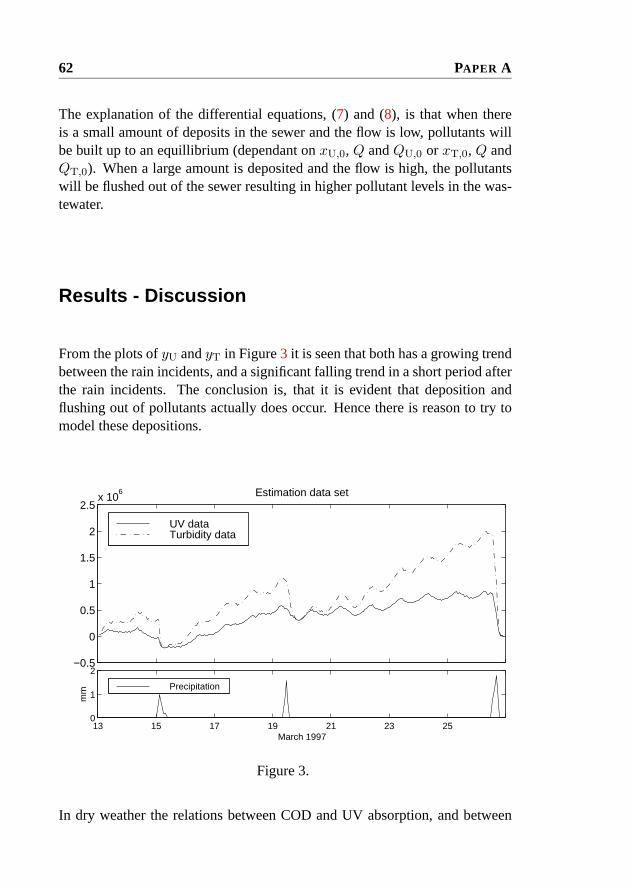
62 PAPER A
The explanation of the differential equations, (7) and (8), is that when thereis a small amount of deposits in the sewer and the flow is low, pollutants willbe built up to an equillibrium (dependant onxU,0, Q andQU,0 or xT,0, Q andQT,0). When a large amount is deposited and the flow is high, the pollutantswill be flushed out of the sewer resulting in higher pollutant levels in the was-tewater.
Results - Discussion
From the plots ofyU andyT in Figure3 it is seen that both has a growing trendbetween the rain incidents, and a significant falling trend in a short period afterthe rain incidents. The conclusion is, that it is evident that deposition andflushing out of pollutants actually does occur. Hence there is reason to try tomodel these depositions.
13 15 17 19 21 23 25 0
1
2
March 1997
mm Precipitation
−0.5
0
0.5
1
1.5
2
2.5x 10
6 Estimation data set
UV data Turbidity data
Figure 3.
In dry weather the relations between COD and UV absorption, and between

Wat. Sci. Tech.,37(12), pp. 87–93, 1998 63
SS and turbidity was found to be:
COD = 5.0mg
l×m−1UV − 26
mgl
SS = 1.52mg
l× FTUTurb− 7.8
mgl
with correlation coefficients 0.90 and 0.85 respectively. These relations aregood during dry weather, but are not suitable in storm situations. Hence insteadof measuring discharge during storms, we model the build-up of pollutantsduring dry weather. This simple approach is reliable if the dry weather load tothe sewer is predictable or constant.
A second order harmonic was found to be reasonable in describing the diurnalprofiles for both UV and turbidity mass flow. In Figure4 results of the massflow estimations are shown with the validation data set. The model is seen todescribe the measurement data reasonably well.
28 29 30 31 1 2 3 4 5 6
0
2
4
6x 10
5
m3 /h
FT
U
March − April 1997
QT
Modelled QT
0
1
2
3x 10
5
m3 /h
m−
1
Validation data set
QU
Modelled QU
Figure 4. Real and modelled UV and turbidity mass flows.
The estimated parameters in (3), (4), (7) and (8) are shown in Table1, and theestimated diurnal profiles forQU andQU are shown in Figure5, and as ex-pected the pollutant load is lowest in the night and the early morning hours andare highest in the afternoon. It is important to notice that the estimated valuesof cU andcT are dependant on the initial values ofxU andxT, respectively.

64 PAPER A
The initial values ofxU were estimated to45× 103m3 ×m−1 for the estima-tion data set and52 × 103m3 ×m−1 for the validation data set. The initialvalues ofxT were estimated to90× 103m3 × FTU for the estimation data setand95× 103m3 × FTU for the validation data set.
a0 = 44.4× 10³m3/h×m−1 c0 = 48.2× 10³m3/h× FTUa1 = −6.54× 10³m3/h×m−1 c1 = −10.3× 10³m3/h× FTUb1 = −2.40× 10³m3/h×m−1 d1 = −2.60× 10³m3/h× FTUa2 = −1.25× 10³m3/h×m−1 c2 = −1.15× 10³m3/h× FTUb2 = 3.81× 10³m3/h×m−1 d2 = 1.98× 10³m3/h× FTUaU = 0.0821h−1 aT = 0.0685h−1
bU = 59.7m−1 bT = 121.5FTUcU = 81.2× 10³m3/h×m−1 cT = 162× 103m3/h× FTU
Table 1.
The values ofaU andaT shows that the UV and turbidity will build up in thesewer with the time constants1/0.0821h = 12.2h and1/0.0685h = 14.6h.This means that after a (considerable) change in the flow, the UV and turbiditymasses in the sewer will reach 63% of the equilibrium in 12.2 and 14.6 hours,respectively.
The estimations of the pollutant masses in the sewer is shown in Figure6. Itis clear that the pollutants are built up in the sewer during dry weather andflushed out during the rain incidents. During the first approximately 24 hoursafter the rain incident the growth is much faster than it was just before the rain,which shows that the level of UV and turbidity at the WWTP is higher duringthe rain periods, than under normal dry weather conditions. After the rain thelevels will be lower at the WWTP, since the depots in the sewer are built upagain.
Conclusions
On-line measurements of UV absorption, turbidity and wastewater flow com-bined with grey-box modelling can be used to identify a model for pollutantconcentrations in the wastewater and the amount of deposits in the sewer sys-
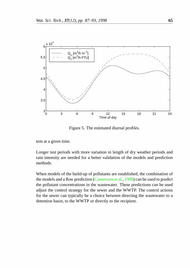
Wat. Sci. Tech.,37(12), pp. 87–93, 1998 65
0 3 6 9 12 15 18 21 243
3.5
4
4.5
5
5.5
6x 10
4
Time of day
QU [m3/h m−1]
QT [m3/h FTU]
Figure 5. The estimated diurnal profiles.
tem at a given time.
Longer test periods with more variation in length of dry weather periods andrain intensity are needed for a better validation of the models and predictionmethods.
When models of the build-up of pollutants are established, the combination ofthe models and a flow prediction (Carstensen et al., 1998) can be used to predictthe pollutant concentrations in the wastewater. These predictions can be usedadjust the control strategy for the sewer and the WWTP. The control actionsfor the sewer can typically be a choice between directing the wastewater to adetention basin, to the WWTP or directly to the recipient.

66 PAPER A
28 29 30 31 1 2 3 4 5 60
1
2
March − April 1997
mm Precipitation
0
0.5
1
1.5
2
2.5x 10
6 Validation data set
xU [m3 m−1]
xT [m3 FTU]
Figure 6. The estimated build up of pollutants in the sewer.

Paper B
Grey box modelling of firstflush and incoming
wastewater at a wastewatertreatment plant.
Published inEnvironmetrics,11(1), pp. 1–12, 2000
B
67


Environmetrics, 11(1),PP. 1–12, 2000 69
Summary
On-line measurements of turbidity, UV absorption and flow in the inlet to aDanish wastewater treatment plant are used to establish a dynamic model ofthe deposition of pollutants in the sewer system and the pollutant mass flowto the treatment plant. The modelling is made using the grey box approach,which is a statistical method that uses known physical relations to formulate themodel. The dynamics of the sewer are modelled by means of continuous timestochastic differential equations combined with dry weather diurnal pollutantmass flows.
Key words:On-line measurements; sewer systems; wastewater treatment plant;dynamic systems; grey box modelling; stochastic differential equations; firstflush; diurnal pollutant load
Introduction
Modelling of sewer systems is necessary to gain a better understanding of thedynamics of the system, and to verify if deposition of pollutants occurs. Ifdeposition occurs then the model can be used to predict and quantify the firstflushes. When the dynamics of the first flushes are quantified, it can be usedto calculate the necessary size of a storage basin in the sewer system or at thewastewater treatment plant.
When modelling sewer systems, these are often described using a configura-tion of storage volumes and pipes with different dimensions. This approachresults in a mathematical model with many parameters and internal states ofthe stores. Unfortunately the data seldom provides sufficient information touniquely identify all parameters.
In this paper a data based grey box modelling approach is used. A grey boxmodel is a stochastic model which only describes the most important physicalrelations. The benefits of this approach are that the resulting model has few pa-rameters and states which are possible to identify, using appropriate statisticalmethods. Due to the small number of parameters, few computational resourcesare needed to estimate the parameters, which makes the parameter estimation
70 PAPER B
applicable for on-line use, e.g. for on-line control purposes (Carstensen et al.,1996).
The present work is based on on-line measurements of UV absorption, turbid-ity and flow. The measurements of UV absorption and turbidity are used toestimate the actual level of chemical oxygen demand (COD) and suspendedsolids (SS) in the wastewater (Kanaya et al., 1985; Ruban et al., 1993; Nowackand Ueberbach, 1995; Matsché and Stumwöhrer, 1996). Based on these dataa model including the diurnal profiles of COD and SS mass flow as well asthe amount of COD and SS deposits in the sewer, is proposed and identified.The model parameters are estimated using one set of data, and cross validatedusing another data set.
The deposits, which are not practically measurable, are states in the model andhence estimated by means of the procedure. By use of the model the estimatedamounts of deposited pollutants in the sewer are identified and shown.
The measurement system
A measuring box, developed by Krüger A/S, Denmark, has been collectingmeasurements from the inlet to the wastewater treatment plant of the town ofSkive in central Jutland, Denmark, in the early spring of 1997. The Krügermeasuring box is a compact and portable unit which consists of a datalog-ger, a Dr. Lange UV absorbance sensor model LXV 109 and a Dr. LangeSOLITAXplus LXV 121 turbidity sensor. Furthermore inlet flow estimates arecollected from the supervisory control and data acquisition (SCADA) systemof the WWTP. The flow estimates are computed in the SCADA system on thebasis of measurements from the inlet pumping station. Off-line measurementsof the precipitation and laboratory analyses of COD and SS are also available.
The influent to Skive WWTP is separated into industrial and municipal waste-water. The sensors are placed in the municipal wastewater.
Environmetrics, 11(1),PP. 1–12, 2000 71
COD and SS
Linear relationships between the concentration of COD denotedCCOD andUV absorption (UV ) and between the concentration of SS denotedCSS andturbidity (Turb) have been suggested by several authors (Kanaya et al., 1985;Ruban et al., 1993; Nowack and Ueberbach, 1995; Matsché and Stumwöhrer,1996), i.e.
CCOD = α UUV + β U (1)
CSS = α TTurb+ β T (2)
whereα U , β U , α T andβ T are constants. The concentrations of COD and SSare measured ingO2/m3 andgSS/m3. The models are calibrated on the basisof laboratory measurements ofCCOD andCSS and the corresponding on-linemeasurements ofUV andTurb. When the concentrations are multiplied bythe wastewater flowQ (in m3/h) the results are the mass flows of COD andSS ingO2/h andgSS/h, respectively.
A dynamical model of the deposited pollutants
It is assumed that pollutants quantified as masses of COD and SS deposit grad-ually in the sewer system and on impervious areas of the catchment in dryweather (low wastewater flow). Similarly, it is assumed that the deposited pol-lutants are flushed out during rain incidents and into the inlet of the treatmentplant. This means that the model does not explicitly describe reactions occur-ring in the sewers, but these processes are in part accounted for through thestatistical calibration of the model.
The deposited amounts of COD and SS are denotedXCOD andXSS , respec-tively. The time derivatives,dXCOD/dt anddXSS/dt are the growth rates atwhich COD and SS are built up in the depots. The growth rates are assumed tobe described by the first order linear differential equations:
dXCOD
dt= aCOD(XCOD − XCOD) + bCOD(Q− Q) (3)
dXSS
dt= aSS(XSS − XSS) + bSS(Q− Q) (4)
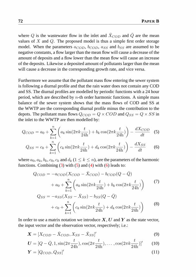
72 PAPER B
whereQ is the wastewater flow in the inlet andXCOD andQ are the meanvalues ofX andQ. The proposed model is thus a simple first order storagemodel. When the parametersaCOD, bCOD, aSS andbSS are assumed to benegative constants, a flow larger than the mean flow will cause a decrease of theamount of deposits and a flow lower than the mean flow will cause an increaseof the deposits. Likewise a deposited amount of pollutants larger than the meanwill cause a decrease in the corresponding growth rate, and vice versa.
Furthermore we assume that the pollutant mass flow entering the sewer systemis following a diurnal profile and that the rain water does not contain any CODand SS. The diurnal profiles are modelled by periodic functions with a 24 hourperiod, which are described byn-th order harmonic functions. A simple massbalance of the sewer system shows that the mass flows of COD and SS atthe WWTP are the corresponding diurnal profile minus the contribution to thedepots. The pollutant mass flowsQCOD = Q×COD andQSS = Q× SS inthe inlet to the WWTP are then modelled by:
QCOD = a0 +n∑k=1
(ak sin(2πk
t
24h) + bk cos(2πk
t
24h))− dXCOD
dt(5)
QSS = c0 +n∑k=1
(ck sin(2πk
t
24h) + dk cos(2πk
t
24h))− dXSS
dt(6)
wherea0, ak, bk, c0, ck anddk (1 ≤ k ≤ n), are the parameters of the harmonicfunctions. Combining (3) with (5) and (4) with (6) leads to:
QCOD = −aCOD(XCOD − XCOD)− bCOD(Q− Q)
+ a0 +n∑k=1
(ak sin(2πk
t
24h) + bk cos(2πk
t
24h))
(7)
QSS = −aSS(XSS − XSS)− bSS(Q− Q)
+ c0 +n∑k=1
(ck sin(2πk
t
24h) + dk cos(2πk
t
24h))
(8)
In order to use a matrix notation we introduceX,U andY as the state vector,the input vector and the observation vector, respectively; i.e.:
X = [XCOD − XCOD, XSS − XSS ]′ (9)
U = [Q− Q, 1, sin(2πt
24h), cos(2π
t
24h), . . . , cos(2πk
t
24h)]′ (10)
Y = [QCOD, QSS ]′ (11)
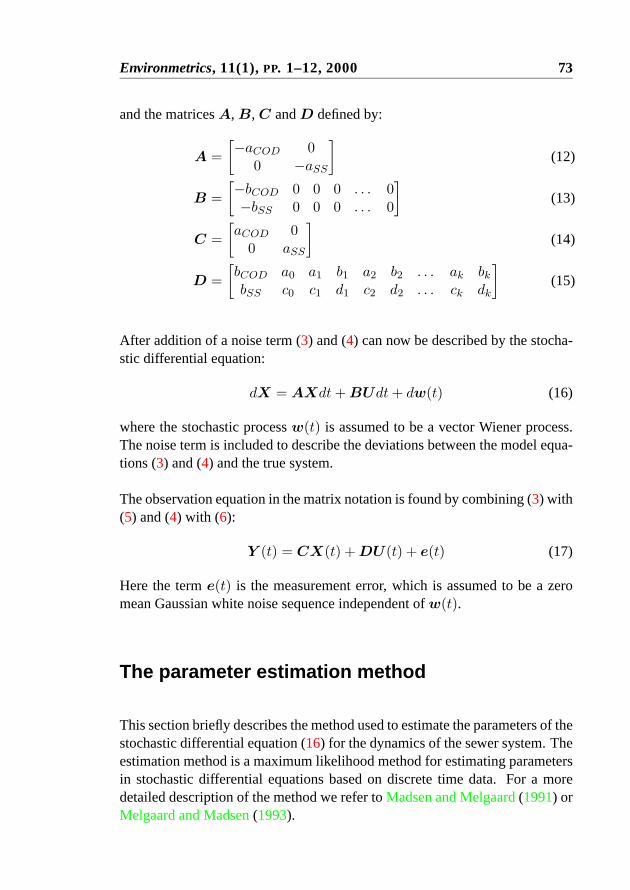
Environmetrics, 11(1),PP. 1–12, 2000 73
and the matricesA,B,C andD defined by:
A =[−aCOD 0
0 −aSS
](12)
B =[−bCOD 0 0 0 . . . 0−bSS 0 0 0 . . . 0
](13)
C =[aCOD 0
0 aSS
](14)
D =[bCOD a0 a1 b1 a2 b2 . . . ak bkbSS c0 c1 d1 c2 d2 . . . ck dk
](15)
After addition of a noise term (3) and (4) can now be described by the stocha-stic differential equation:
dX = AXdt+BUdt+ dw(t) (16)
where the stochastic processw(t) is assumed to be a vector Wiener process.The noise term is included to describe the deviations between the model equa-tions (3) and (4) and the true system.
The observation equation in the matrix notation is found by combining (3) with(5) and (4) with (6):
Y (t) = CX(t) +DU(t) + e(t) (17)
Here the terme(t) is the measurement error, which is assumed to be a zeromean Gaussian white noise sequence independent ofw(t).
The parameter estimation method
This section briefly describes the method used to estimate the parameters of thestochastic differential equation (16) for the dynamics of the sewer system. Theestimation method is a maximum likelihood method for estimating parametersin stochastic differential equations based on discrete time data. For a moredetailed description of the method we refer toMadsen and Melgaard(1991) orMelgaard and Madsen(1993).
74 PAPER B
The observations are given in discrete time, and, in order to simplify the nota-tion, we assume that the time indext belongs to the set{0, 1, 2, ..., N}, whereN is the number of observations. Introduce
Y(t) = [Y (t),Y (t− 1), . . . ,Y (1),Y (0)]′ (18)
i.e.Y(t) is a vector containing all the observations up to and including timet.
Using the matrix notation the continuous time stochastic differential equationdescribing the dynamics of the sewer system can be written as the so-called Itôdifferential equation (Øksendal, 1995)
dX(t) = f(X,U , t)dt+G(U , t)dw(t) (19)
whereX is the state vector,U an input (e.g. control) vector,w a vectorstandard Wiener process (see e.g.Kloeden and Platen(1995)), andf andG areknown functions. The matrixG(U, t) describes any input or time dependentvariation related to how the variation generated by the Wiener process entersthe system.
For the observations we assume the discrete time relation
Y (t) = h(X,U , t) + e(t) (20)
wheree(t) is assumed to be a Gaussian white noise sequence independent ofw. All the unknown parameters, denoted by the vectorθ, are embedded in thecontinuous-discrete time state space model (equations (19) and (20)).
The likelihood function is the joint probability density of all the observationsassuming that the parameters are known, i.e.
L′(θ;Y(N)) = p(Y(N)|θ)= p(Y (N)|Y(N − 1),θ)p(Y(N − 1)|θ)
=( N∏t=1
p(Y (t)|Y(t− 1),θ))p(Y (0)|θ)
(21)
where successive applications of the ruleP (A∩B) = P (A|B)P (B) are usedto express the likelihood function as a product of conditional densities.
In order to evaluate the likelihood function it is assumed that all the conditionaldensities are Gaussian. In the case of a linear state space model as described

Environmetrics, 11(1),PP. 1–12, 2000 75
by (16) and (17), it is easily shown that the conditional densities are actuallyGaussian (Madsen and Melgaard, 1991). In the more general non-linear casethe Gaussian assumption is an approximation.
The Gaussian distribution is completely characterized by the mean and covari-ance. Hence, in order to parameterize the conditional distribution, we intro-duce the conditional mean and the conditional covariance as
Y (t|t− 1) = E[Y (t)|Y(t− 1),θ] and
R(t|t− 1) = V [Y (t)|Y(t− 1),θ](22)
respectively. It should be noted that these correspond to the one-step predictionand the associated covariance, respectively. Furthermore, it is convenient tointroduce the one-step prediction error (or innovation)
ε(t) = Y (t)− Y (t|t− 1) (23)
For calculating the one-step prediction and its variance, an iterated extendedKalman filter is used. The extended Kalman filter is simply based on a line-arization of the system equation (19) around the current estimate of the state(seeGelb (1974)). The iterated extended Kalman filter is obtained by localiterations of the linearization over a single sample period.
Using (21) – (23) the conditional likelihood function (conditioned onY (0))becomes
L(θ;Y(N))
=N∏t=1
((2π)−m/2 detR(t|t− 1)−1/2 exp(−1
2ε(t)′R(t|t− 1)−1ε(t))
) (24)
wherem is the dimension of theY vector. Traditionally the logarithm of theconditional likelihood function is considered
logL(θ;Y(N))
= −12
N∑t=1
(log detR(t|t− 1) + ε(t)′R(t|t− 1)−1ε(t)
)+ const
(25)
The maximum likelihood estimate (ML-estimate) is the setθ, which maxi-mizes the likelihood function. Since it is not, in general, possible to optimize
76 PAPER B
the likelihood function analytically, a numerical method has to be used. Areasonable method is the quasi-Newton method.
An estimate of the uncertainty of the parameters is obtained by the fact that theML-estimator is asymptotically normally distributed with meanθ and covari-ance
D = H−1 (26)
where the matrixH is given by
{hlk} = −E[
∂2
∂θl∂θklogL(θ;Y(N))
](27)
An estimate ofD is obtained by equating the observed value with its expecta-tion and applying
{hlk} ≈ −(
∂2
∂θl∂θklogL(θ;Y(N))
)|θ=θ
(28)
The above equation can be used for estimating the variance of the parameterestimates. The variances serves as a basis for calculating t-test values for testunder the hypothesis that the parameter is equal to zero. Finally, the correla-tion between the parameter estimates is readily found based on the covariancematrixD.
Results and Discussion
In dry weather the relations between COD and UV absorption and between SSand turbidity were found by regression analysis to be:
CCOD = 5.0g
m3m−1UV − 26
gm3
(29)
CSS = 1.52g
m3FTUTurb− 7.8
gm3
(30)
with degrees of explanationR2 = 0.90 andR2 = 0.85, respectively. In dryweather equations (29) and (30) describe the relations well, and it is assumedthat it is reasonable to extrapolate to rainy situations. More thorough research

Environmetrics, 11(1),PP. 1–12, 2000 77
will have to be carried out to refine the relationships between the measurementsof UV absorption and turbidity, and COD and SS, respectively. This investi-gation could include flow dependent parameter values. Such an approach willincrease the need for laboratory analysis of COD and SS enormously.
The parameters in the model were estimated using the CTLSM program (Mad-sen and Melgaard, 1991; Melgaard and Madsen, 1991). Different orders of theharmonic functions were tried, and it was found that a second order harmonicwas reasonable in describing the diurnal profiles for both COD and SS massflow. The estimated parameters are shown in Table1, together with the estima-ted standard deviations of the parameter estimates.
It was found thatc2 was not significantly different from zero, and it was there-fore excluded from the final estimation.
In the model presented it is not possible to estimate the mean level of the non-measured deposited pollutantsXCOD andXSS . In the estimations these werefixed at zero, meaning thatXCOD andXSS are differences from unknownmean values. This does not put any limitations on the use of the model, as it isstill possible to quantify the amount of pollutants in a first flush.
Validation of the resulting model was done by cross-validation, i.e. by apply-ing the model on a data set (the validation data set), which differs from thatused for the parameter estimation. Using all the estimated parameter values,except for the initial states, the initial values of the states for the validationdata set were found by the estimation software. In Figures1 and2 the mea-sured and simulated pollutant mass flows are shown. They are seen to be ingood agreement. Furthermore tests on the white noise assumption based onthe autocorrelations and on the cumulative residual periodograms were carriedout. It was seen that the white noise assumptions were not perfectly satisfied,but since the cross-validations shown in Figures1 and 2 are very fine, it isconcluded that the model describes the data well.
In Figures3 and4 the estimated amounts of deposited COD and SS are shownfor the estimation data set and for the validation data set, and it is clear thatCOD and SS are deposited in dry weather periods and flushed out during rainincidents. From Figure4 it appears that the amount of COD first flush duringthe rain incident on April 3rd is approximately2500 kgO2 and that the SSfirst flush is approximately1800 kgSS. A comparison of these amounts with

78 PAPER B
Par
amet
eraCOD
b COD
a0
a1
b 1a
2b 2
Uni
th−
1kgO
2
m3
kgO
2
hkgO
2
hkgO
2
hkgO
2
hkgO
2
h
Est
imat
e-0
.054
32-0
.296
919
8.3
-26.
58-1
6.05
-6.7
1020
.76
Sta
ndar
dde
viat
ion
0.00
378
0.00
411.
21.
501.
621.
560
1.47
Par
amet
eraSS
b SS
c 0c 1
d1
c 2d
2
Uni
th−
1kgS
Sm
3kgS
Sh
kgS
Sh
kgS
Sh
kgS
Sh
kgS
Sh
Est
imat
e-0
.035
97-0
.196
262
.14
-12.
27-6
.008
–2.
713
Sta
ndar
dde
viat
ion
0.00
259
0.00
320.
711.
091.
061
–1.
054
Table 1. Maximum likelihood estimates of the parameters of the system.
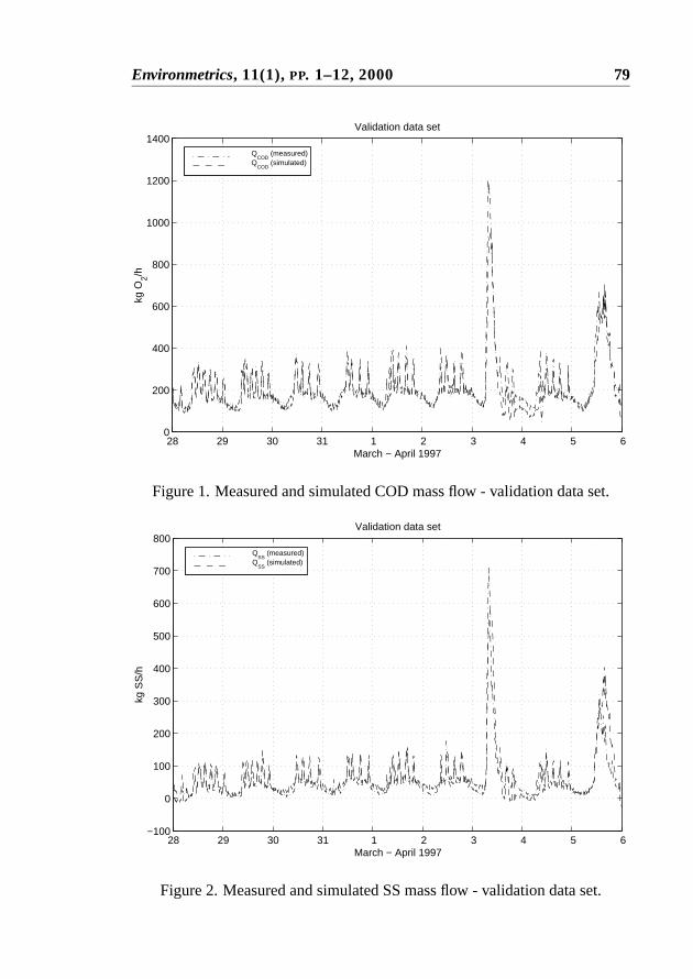
Environmetrics, 11(1),PP. 1–12, 2000 79
28 29 30 31 1 2 3 4 5 60
200
400
600
800
1000
1200
1400
March − April 1997
kg O
2/hValidation data set
QCOD
(measured) Q
COD (simulated)
Figure 1. Measured and simulated COD mass flow - validation data set.
28 29 30 31 1 2 3 4 5 6−100
0
100
200
300
400
500
600
700
800
March − April 1997
kg S
S/h
Validation data set
QSS
(measured) Q
SS (simulated)
Figure 2. Measured and simulated SS mass flow - validation data set.
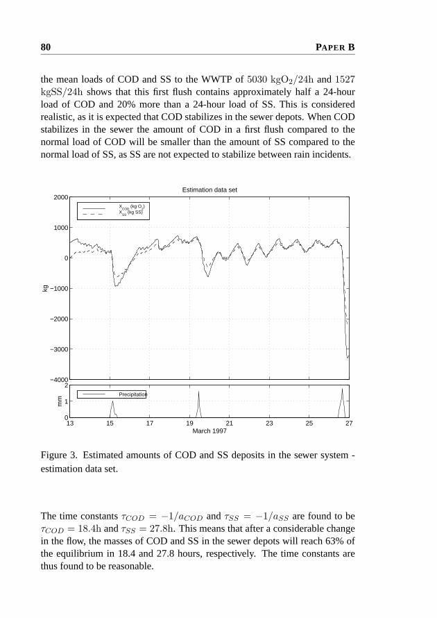
80 PAPER B
the mean loads of COD and SS to the WWTP of5030 kgO2/24h and1527kgSS/24h shows that this first flush contains approximately half a 24-hourload of COD and 20% more than a 24-hour load of SS. This is consideredrealistic, as it is expected that COD stabilizes in the sewer depots. When CODstabilizes in the sewer the amount of COD in a first flush compared to thenormal load of COD will be smaller than the amount of SS compared to thenormal load of SS, as SS are not expected to stabilize between rain incidents.
13 15 17 19 21 23 25 270
1
2
March 1997
mm
Precipitation
−4000
−3000
−2000
−1000
0
1000
2000
kg
Estimation data set
XCOD
(kg O2)
XSS
(kg SS)
Figure 3. Estimated amounts of COD and SS deposits in the sewer system -estimation data set.
The time constantsτCOD = −1/aCOD andτSS = −1/aSS are found to beτCOD = 18.4h andτSS = 27.8h. This means that after a considerable changein the flow, the masses of COD and SS in the sewer depots will reach 63% ofthe equilibrium in 18.4 and 27.8 hours, respectively. The time constants arethus found to be reasonable.

Environmetrics, 11(1),PP. 1–12, 2000 81
28 29 30 31 1 2 3 4 5 60
1
2
March − April 1997
mm
Precipitation
−4000
−3000
−2000
−1000
0
1000
2000kg
Validation data set
XCOD
(kg O2)
XSS
(kg SS)
Figure 4. Estimated amounts of COD and SS deposits in the sewer system -validation data set.
Conclusion
In this paper a stochastic grey box model of the deposition of pollutants in thesewer system and on impervious areas of the catchment is proposed. Further-more, the model provides a characterization of the influent wastewater to theWWTP. The parameters of the model are estimated using the maximum like-lihood method. The modelling is based on measurements of concentrations ofCOD and SS, which are calculated from measurements of UV absorption andturbidity. It is concluded that the models, which relate the measurements ofUV absorption and turbidity to COD and SS concentrations, describe the rela-tions well in dry weather situations, and it is assumed that it is reasonable toextrapolate to rainy conditions.
Using the grey box approach, it is possible to identify a model for a com-

82 PAPER B
plex dynamical system based on simple physical assumptions combined withstatistical modelling tools. The model is formulated in continuous time withdiscrete time measurements and due to the rather small number of parameters,the model is operational for on-line applications.
The model makes it possible to estimate the amount of COD and SS in a firstflush during a rain incident. It is found that these amounts are dependent on thetime interval since the previous rain event and on the intensity of the currentrain.
Acknowledgements
The authors wish to thank Skive WWTP for its cooperation during the datacollection and for making the laboratory analyses, and Henrik A. Thomsenand Kenneth Kisbye for their kind assistance in the data collection. Thanks arealso due to the Danish Academy of Technical Sciences for funding the projectin which the present work has been carried out, under grant EF-623.

Paper C
Grey-box modelling ofpollutant loads from a sewer
system.Published inUrbanWater,1(1), pp. 71–78, 1999
C
83

UrbanWater, 1(1), PP. 71–78, 1999 85
Abstract
Using a compact measuring unit with on-line meters for UV absorption andturbidity, it is possible to determine concentrations of organic load (chemicaloxygen demand and suspended solids) anywhere in a sewer system. Whenmeasurements of the flow are available as well, the pollutant mass flow at themeasuring point can be calculated.
The measured data are used to estimate different models describing the loadof pollutants in the sewer. A comparison of the models shows that a grey-boxmodel is most informative and best in terms measured by the multiple corre-lation coefficient. The grey-box model is a state-space model, where the staterepresents the actual amount of deposition in the sewer, and the output fromthe model is the pollutant mass flow to the wastewater treatment plant. Themodel is formulated by means of stochastic differential equations. Harmonicfunctions are used to describe the dry weather diurnal load profiles. It is foundthat the accumulation of deposits in the sewer depends on previous rain eventsand flows.
By means of on-line use of the grey-box models, it is possible to predict theamount of pollutants in a first flush at any time, and hence from the capacityof the plant to decide if and when the available detention basin is to be usedfor storage of wastewater. The mass flow models comprise an important im-provement of the integrated control of sewer and wastewater treatment plantincluding control of equalisation basins in the sewer system. Further improve-ments are expected by the introduction of an additive model where dry weathersituations and storm situations are modelled separately before addition to theresulting model.
Key words: Pollutant deposition, sewer system, first flush, grey-box models,statistical identification, on-line measurements.
Introduction
On-line measurements of organic pollution in terms of biological, chemicalor total oxygen demand (BOD, COD or TOD) and suspended solids (SS) by

86 PAPER C
means of UV absorbance and turbidity sensors are now well described (Dobbset al., 1972; Mrkva, 1975; Kanaya et al., 1985; Ruban et al., 1993; Nowackand Ueberbach, 1995; Matsché and Stumwöhrer, 1996; Reynolds and Ahmad,1997; Wass et al., 1997). When on-line measurements of COD and SS areavailable a better characterization of the wastewater can be achieved, and thisleads to a better understanding of the processes in the sewer system.
The sewer system is often modelled by means of deterministic modelling as aconfiguration of storage volumes connected with pipes of different dimensions(Mark et al., 1995; Dempsey et al., 1997; Heip et al., 1997; van Luijtelaarand Rebergen, 1997). As these models are formulated as a large collectionof differential equations with many parameters, it is difficult to estimate theparameters on the basis of available measurements.
Data based models are also common in the literature (Capodaglio, 1994; Delleurand Gyasi-Agyei, 1994; Ruan and Wiggers, 1997; Young et al., 1997). Thesemodels have few parameters, which can then be estimated on the basis of avail-able data. However, as the models are most often formulated in discrete time,the parameter estimates depend on the sampling time.
In this paper a data based grey-box modelling approach is used. A grey-boxmodel is a physically based macroscopic model with stochastic terms to countin uncertainties in model formulation and measurement values. The introduc-tion of stochastic terms enables maximum likelihood estimation of the modelparameters. The maximum likelihood method provides estimates of the vari-ances of the parameter estimates, which are used to evaluate the uncertainty ofthe parameters. The proposed models are formulated here in continuous time.Measurements of pollutant mass flows in the inlet to a wastewater treatmentplant (WWTP) are modelled by means of models of differing complexity. Pol-lutant deposition in the sewer can for instance be included, to make it possibleto quantify the amounts of pollutants in a first flush.
The measurement system
A compact portable measuring box, developed by Krüger A/S, Denmark, hasbeen used to collect measurements of UV absorption and turbidity from theinlet to the Aalborg East wastewater treatment plant in Northern Jutland, Den-
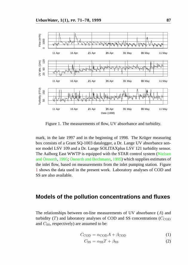
UrbanWater, 1(1), PP. 71–78, 1999 87
Flo
w (
m³/
h)
010
00
11 Apr 16 Apr 21 Apr�
26 Apr�
01 May�
06 May�
11 May
UV
abs
. (1/
m)
2060
120
11 Apr 16 Apr 21 Apr�
26 Apr�
01 May�
06 May�
11 May
Date (1998)
Tur
bidi
ty (
FT
U)
5015
0
11 Apr 16 Apr 21 Apr�
26 Apr�
01 May�
06 May�
11 May
Figure 1. The measurements of flow, UV absorbance and turbidity.
mark, in the late 1997 and in the beginning of 1998. The Krüger measuringbox consists of a Grant SQ-1003 datalogger, a Dr. Lange UV absorbance sen-sor model LSV 109 and a Dr. Lange SOLITAXplus LSV 121 turbidity sensor.The Aalborg East WWTP is equipped with the STAR control system (Nielsenand Önnerth, 1995; Önnerth and Bechmann, 1995) which supplies estimates ofthe inlet flow, based on measurements from the inlet pumping station. Figure1 shows the data used in the present work. Laboratory analyses of COD andSS are also available.
Models of the pollution concentrations and fluxes
The relationships between on-line measurements of UV absorbance (A) andturbidity (T ) and laboratory analyses of COD and SS concentrations (CCOD
andCSS, respectively) are assumed to be:
CCOD = αCODA+ βCOD (1)
CSS = αSST + βSS (2)

88 PAPER C
whereαCOD, βCOD, αSS andβSS are parameters, which have to be estima-ted on the basis of measurements ofCCOD, CSS, A andT , as the parame-ters depend on the actual operating conditions and the wastewater composition(Dobbs et al., 1972; Mrkva, 1975; Kanaya et al., 1985; Ruban et al., 1993;Nowack and Ueberbach, 1995; Matsché and Stumwöhrer, 1996; Reynolds andAhmad, 1997; Wass et al., 1997). When these parameters are estimated, it ispossible to consider the observation at timet of pollution flux:
y(t) = Q(t)C(t) (3)
with Q(t) andC(t) denoting the flow and the pollution concentration (CCOD
orCSS), respectively. This quantity can be modelled using:
y(t) = y(t) + ε(t) (4)
Herey(t) is the predictable part of the model, and the residualε(t) is a stocha-stic part, which is the difference between the data observed and the predictionobtained from the model.
The first approach considered is to model the pollution flux using a fixed diur-nal profile expressed as ann-th order harmonic function with a 24 hour period(model 1):
y(t) = a0 +n∑k=1
(ak sin(2πk
t
24h) + bk cos(2πk
t
24h))
(5)
wherea0, ak, andbk (1 ≤ k ≤ n), are the unknown parameters.
Another approach is to model the flux as a mean value and a term proportionalto the flow (model 2):
y(t) = c0 + c1Q(t) (6)
wherec0 andc1 are positive parameters.
These two approaches can be combined to (model 3):
y(t) = a0 +n∑k=1
(ak sin(2πk
t
24h) + bk cos(2πk
t
24h))
+ cQ(t) (7)

UrbanWater, 1(1), PP. 71–78, 1999 89
Note that the parameter values of the Fourier expansion in equations (5) and(7) are in general not the same, as some of the harmonic variation iny(t) ismost likely explained by the harmonic variation ofcQ(t).
These approaches all result in static models.
The final approach considered is model 4 which is a dynamic model formulatedas a state-space model. This model takes the deposition of pollutants in thesewer system and on impervious areas of the catchment area into account.
The model is based on the assumption that pollutants deposit gradually in dryweather and that the deposited pollutants are flushed out during rain incidentsand into the inlet of the treatment plant. Letx(t) denote the deposition of pol-lutants at timet. Then a simple first order linear ordinary differential equation:
dxdt
= a(x− x) + b(Q− Q) (8)
can be used to describe the dynamics of the pollution deposition. The timederivative ofx is the estimated growth rate at which pollution is built up in thesewer, andx andQ are the mean values ofx andQ. The parametersa andb are assumed to be negative, and hence a flow larger than the average flowduring the period will decrease the growth rate and a flow lower than the meanflow will increase the growth rate. Similarly a deposited amount larger thanthe mean will decrease the growth rate, and vice versa.
The pollution flux observed at the measuring point in the inlet to the WWTP, isassumed to consist of a fixed diurnal profile, which describes the pollutants thatenter the sewer system, minus a contribution to the depositions in the sewer.This is formulated in the observation equation:
y(t) = a0 +n∑k=1
(ak sin(2πk
t
24h) + bk cos(2πk
t
24h))− dx
dt
= a0 +n∑k=1
(ak sin(2πk
t
24h) + bk cos(2πk
t
24h))
− a(x− x)− b(Q− Q)
(9)
Besides a better description of the available data, this approach also providesinformation about the practically unmeasureable amount of deposits in the
90 PAPER C
sewer and impervious areas of the catchment. Hence, besides the parameterestimates, the model also provides an estimate ofx − x. This means that themodel does not give information about the actual deposition levelx, but onlyabout the difference from the mean level of deposition. This does not pose anypractical limitations on the use of the model, as, for instance, it is still possibleto quantify the amount of pollutants in a first flush.
All the proposed pollution flux models can be applied to both SS and CODflux.
Estimation methods
The parameters of the concentration models (1) and (2) as well as the param-eters of the static pollution flux models (5), (6), and (7), can be estimated byordinary least squares methods, as these models are all linear in the parameters.
The method used to estimate the parameters of the dynamic pollution flux mo-del (4) and (8) – (9) is a maximum likelihood method for estimating parametersin stochastic differential equations based on discrete time data given by (4).For a more detailed description of the method refer toMadsen and Melgaard(1991) or Melgaard and Madsen(1993).
In order to use the maximum likelihood method, some stochastic terms haveto be introduced. Hence, the first order differential equation (8) turns into astochastic differential equation, where the continuous time equation describingthe dynamics of the pollution deposition can be written as the so-called Itôdifferential equation (Øksendal, 1995)
dx(t) = f(x, u, t)dt+ g(u, t)dw(t) (10)
wherex is the state variable,u an input (e.g. control) variable,w a standardWiener process (see e.g.Kloeden and Platen(1995)), andf andg are knownfunctions. The functiong(u, t) describes any input or time dependent varia-tion related to how the variation generated by the Wiener process enters thesystem. Note, that in order to illustrate the flexibility of the method equation(10) represents a generalization of the ordinary state equation (8).

UrbanWater, 1(1), PP. 71–78, 1999 91
For the observations we assume the discrete time relation
y(t) = h(x, u, t) + e(t) (11)
wheree(t) is assumed to be a Gaussian white noise sequence independent ofw, which can be seen as a generalization of (4) and (9). All the unknownparameters, denoted by the vectorθ, are embedded in the continuous-discretetime state space model (equations (10) and (11)).
The observations are given in discrete time, and, in order to simplify the nota-tion, we assume that the time indext belongs to the set{0, 1, 2, ..., N}, whereN is the number of observations. Introducing
Y(t) = [y(t), y(t− 1), . . . , y(1), y(0)]′ (12)
i.e. Y(t) is a vector containing all the observations up to and including timet, the likelihood function is the joint probability density of all the observationsassuming that the parameters are known, i.e.
L′(θ;Y(N)) = p(Y(N)|θ)= p(y(N)|Y(N − 1),θ)p(Y(N − 1)|θ)
=( N∏t=1
p(y(t)|Y(t− 1),θ))p(y(0)|θ)
(13)
where successive applications of the ruleP (A∩B) = P (A|B)P (B) are usedto express the likelihood function as a product of conditional densities.
In order to evaluate the likelihood function it is assumed that all the conditionaldensities are Gaussian. In the case of a linear state space model as describedby (4) and (8) – (9), it is easily shown that the conditional densities are actuallyGaussian (Madsen and Melgaard, 1991). In the more general non-linear casethe Gaussian assumption is an approximation.
The Gaussian distribution is completely characterized by the mean and covari-ance. Hence, in order to parameterize the conditional distribution, we intro-duce the conditional mean and the conditional variance as
y(t|t− 1) = E[y(t)|Y(t− 1),θ] and
R(t|t− 1) = V [y(t)|Y(t− 1),θ](14)

92 PAPER C
respectively. It should be noted that these correspond to the one-step predic-tion and the associated variance, respectively. Furthermore, it is convenient tointroduce the one-step ahead prediction error (or innovation)
ε(t) = y(t)− y(t|t− 1) (15)
For calculating the one-step ahead prediction and its variance, an iterated ex-tended Kalman filter is used. The extended Kalman filter is simply based ona linearization of the system equation (10) around the current estimate of thestate (seeGelb (1974)). The iterated extended Kalman filter is obtained bylocal iterations of the linearization over a single sample period.
Using (13) – (15) the conditional likelihood function (conditioned ony(0))becomes
L(θ;Y(N)) =N∏t=1
(1√
2π√R(t|t− 1)
exp(− ε(t)2
2R(t|t− 1))
)(16)
Traditionally, the logarithm of the conditional likelihood function is considered
logL(θ;Y(N)) = −12
N∑t=1
(logR(t|t− 1) +
ε(t)2
R(t|t− 1)
)+ const (17)
The maximum likelihood estimate (ML-estimate) is the setθ, which maxi-mizes the likelihood function. Since it is not, in general, possible to optimizethe likelihood function analytically, a numerical method has to be used. Areasonable method is the quasi-Newton method.
An estimate of the uncertainty of the parameters is obtained by the fact that theML-estimator is asymptotically normally distributed with meanθ and covari-ance
D = H−1 (18)
where the matrixH is given by
{hlk} = −E[
∂2
∂θl∂θklogL(θ;Y(N))
](19)

UrbanWater, 1(1), PP. 71–78, 1999 93
An estimate ofD is obtained by equating the observed value with its expecta-tion and applying
{hlk} ≈ −(
∂2
∂θl∂θklogL(θ;Y(N))
)|θ=θ
(20)
The above equation can be used for estimating the variance of the parameterestimates. The variances serve as a basis for calculating t-test values for testunder the hypothesis that the parameter is equal to zero. Finally, the correla-tion between the parameter estimates is readily found, based on the covariancematrixD.
The estimation methods are implemented in the CTLSM program, which areavailable from http://www.imm.dtu.dk/∼hm/.
Results and discussion
The parameters of equations (1) and (2) are found by linear regression. Itturned out thatβCOD andβSS were insignificant, and therefore they were eli-minated in the final estimation. The estimated parameters and their standarddeviations are shown in Table1. The degrees of explanations (multiple corre-lation coefficients) of the COD and SS concentration models areR2 = 0.98andR2 = 0.97, respectively.
Parameter αCOD βCOD αSS βSS
Unit gO2/m3
m−1 gO2/m3 gSS/m3
FTU gSS/m3
Estimate 10.57 – 3.05 –Standard deviation 0.40 – 0.13 –
Table 1. Parameters of equations (1) and (2). Theβ parameters are insignifi-cant and are therefore not estimated.
For the models, which include a diurnal profile modelled as a harmonic func-tion (models 1, 3, and 4), it was found that second order harmonic functionswere suitable, as the higher order coefficients were insignificant. In Tables2and3 it can be seen that some of the parameters of the harmonic functions are

94 PAPER C
Model1
Par
amet
era
0a
1b 1
a2
b 2U
nit
kgO
2
hkgO
2
hkgO
2
hkgO
2
hkgO
2
h
Est
imat
e44
3.5
-148
.6-3
9.22
17.9
453
.94
Sta
ndar
dde
viat
ion
3.8
5.34
5.34
5.34
5.34
Model2P
aram
eter
c 0c 1
Uni
tkgO
2
hkgO
2
m3
Est
imat
e19
0.1
0.34
64S
tand
ard
devi
atio
n10
.30.
0130
Model3
Par
amet
era
0a
1b 1
a2
b 2c
Uni
tkgO
2
hkgO
2
hkgO
2
hkgO
2
hkgO
2
hkgO
2
m3
Est
imat
e27
0.8
-114
.3-2
9.29
19.2
536
.04
0.23
61S
tand
ard
devi
atio
n9.
45.
074.
794.
764.
850.
0120
Model4
Par
amet
era
ba
0a
1b 1
a2
b 2U
nit
h−1
kgO
2
m3
kgO
2
hkgO
2
hkgO
2
hkgO
2
hkgO
2
h
Est
imat
e-0
.087
75-0
.444
844
4.4
-93.
501.
403
24.6
722
.69
Sta
ndar
dde
viat
ion
0.00
864
0.01
753.
04.
654.
690
4.12
4.34
Table 2. Parameter estimates of the COD flux models.

UrbanWater, 1(1), PP. 71–78, 1999 95
Model1P
aram
eter
a0
a1
b 1a
2b 2
Uni
tkgS
Sh
kgS
Sh
kgS
Sh
kgS
Sh
kgS
Sh
Est
imat
e19
8.8
-65.
91-1
6.62
-10.
5532
.10
Sta
ndar
dde
viat
ion
3.3
4.70
4.70
4.70
4.70
Model2
Par
amet
erc 0
c 1U
nit
kgS
Sh
kgS
Sm
3
Est
imat
e-7
7.11
0.37
72S
tand
ard
devi
atio
n5.
250.
0066
Model3
Par
amet
era
0a
1b 1
a2
b 2c
Uni
tkgS
Sh
kgS
Sh
kgS
Sh
kgS
Sh
kgS
Sh
kgS
Sm
3
Est
imat
e-6
7.96
-12.
96-1
.268
-8.5
364.
445
0.36
47S
tand
ard
devi
atio
n5.
603.
012.
846
2.83
02.
882
0.00
71
Model4
Par
amet
era
SS
b SS
a0
a1
b 1a
2b 2
Uni
th−
1kgS
Sm
3kgS
Sh
kgS
Sh
kgS
Sh
kgS
Sh
kgS
Sh
Est
imat
e-0
.011
92-0
.414
720
4.3
-3.9
454.
002
-6.3
57-0
.162
7S
tand
ard
devi
atio
n0.
0009
00.
0086
1.7
2.66
32.
429
2.33
92.
476
Table 3. Parameter estimates of the SS flux models.

96 PAPER C
insignificant, as their estimated values are smaller or comparable in absolutevalues to their estimated standard deviations. Especiallyb1 of COD flux model3, b1 of SS flux model 3 andb2 of SS flux model 4 are very uncertain. Usuallyinsignificant parameters should be excluded from the final estimation, to makethe estimation of the remaining parameters better. However, we have chosento include these parameters for comparison with the other models.
Comparison plots of measured and modelled pollution fluxes of the 4 modelsare shown in Figures2, 3, 4, and5. Note, that the modelled pollution fluxesshown in the figures are not one-step ahead predictions, but simulations fromthe estimated models. The simulations are based only on the measured input tothe models, which is time of day (models 1, 3, and 4) and inlet flow (models 2,3, and 4). In Tables2 and3 the parameter estimates of the proposed models arelisted, and in Table4 the correlations between measured and simulated fluxesR2 of the models are listed.
Model R2
COD model SS model
1 0.39 0.152 0.32 0.693 0.51 0.694 0.61 0.76
Table 4. Degrees of explanation of the different models.
When comparing Figures2, 3, 4 and5, it is seen that the simple harmonic mo-del 1 is good at describing most of the dry weather situations, but not the wetweather situations. Models 2, 3 and 4 are better than model 1 at following thepeaks in pollution flux in wet weather, as they include a term proportional tothe flow. Besides a better correlation between measured and modelled pollu-tant fluxes expressed by the degree of explanationR2, application of the dyna-mic model provides information about the pollutant depositions in the sewer.In Figure 6 the estimated deviations from the mean levels of COD and SSdeposits are shown. From this figure it is seen that pollutants build up in thesewer during dry weather periods and are flushed out during rain. The amountsof deposits in a first flush can also be quantified on the basis of Figure6: Thefirst and second rain incidents contain approximately 3000 kgO2 (COD) and6000 kgSS which are 14% and 63% of the diurnal load of COD and SS, re-

UrbanWater, 1(1), PP. 71–78, 1999 97
spectively. As it is expected that deposited COD stabilizes in the sewer this isconsidered realistic. The stabilization of COD will lead to a smaller amountof COD in a first flush compared to the normal load of COD than the amountof SS compared to the normal load of SS, as deposited SS are not expected tostabilize in the sewer.
The time constants of the dynamic COD and SS models are−1/a = 11.4h and−1/a = 83.9h, respectively. This means that after a considerable change inthe flow, the COD and SS depositions will reach 63% of the steady state levelin 11.4 and 83.9 hours, respectively. The dynamics of the COD deposition isthus about 7 times faster than the dynamics of the SS deposition.
As the data used for estimating the models are dominated by dry weather situ-ations, the fluxes are underestimated during rainful events. A separation of themodels into dry weather models and storm models, which are added to eachother, might be a significant improvement.
Conclusions
Linear relationships between UV absorption and COD and between turbidityand SS are derived. These relationships are used to compute the COD andSS concentrations from on-line measurements of UV absorption and turbidity.Using available measurements of the flow in the inlet to Aalborg East WWTPthe pollution flows of COD and SS are used to estimate models of differingcomplexity. It is shown that the estimated dynamic grey-box models, whichinclude the deposition and flush out of pollutant masses in the sewer, describethe data better than the other models proposed. Furthermore, these dynamicmodels estimate the amounts of deposits in the sewer at any time. Herebythe amounts of pollutants in a first flush are found. This information is veryuseful when control algorithms for the use of the available detention basin atthe WWTP are designed. However, when the models are to be used to enablebetter operational control of available detention basins, predictions of the was-tewater flow to the WWTP are required. When flow forecasts are available, themodels suggested can be used to predict the pollutant load with the same timehorizon as the flow predictions.
With degrees of explanation (multiple correlation coefficients)R2 = 0.76 and

98 PAPER C
Date (1998)
CO
D fl
ux (
kg O
2 / h
)
020
060
010
0014
00
11 Apr 16 Apr 21 Apr 26 Apr 01 May 06 May 11 May
Date (1998)
SS
flux
(kg
SS
/ h)
020
060
010
00
11 Apr 16 Apr 21 Apr 26 Apr 01 May 06 May 11 May
Figure 2. The pollutant flux modelled as a diurnal profile. Solid lines: mea-sured flux, dashed lines: modelled flux.
Date (1998)
CO
D fl
ux (
kg O
2 / h
)
020
060
010
0014
00
11 Apr 16 Apr 21 Apr 26 Apr 01 May 06 May 11 May
Date (1998)
SS
flux
(kg
SS
/ h)
020
060
010
00
11 Apr 16 Apr 21 Apr 26 Apr 01 May 06 May 11 May
Figure 3. The pollutant flux modelled as proportional to the flow. Solid lines:measured flux, dashed lines: modelled flux.
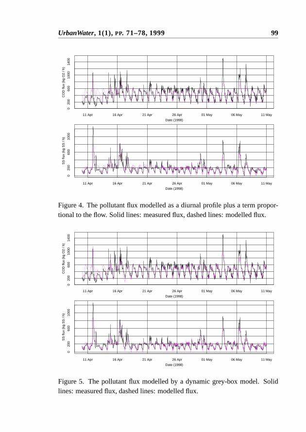
UrbanWater, 1(1), PP. 71–78, 1999 99
Date (1998)
CO
D fl
ux (
kg O
2 / h
)
020
060
010
0014
00
11 Apr 16 Apr 21 Apr 26 Apr 01 May 06 May 11 May
Date (1998)
SS
flux
(kg
SS
/ h)
020
060
010
00
11 Apr 16 Apr 21 Apr 26 Apr 01 May 06 May 11 May
Figure 4. The pollutant flux modelled as a diurnal profile plus a term propor-tional to the flow. Solid lines: measured flux, dashed lines: modelled flux.
Date (1998)
CO
D fl
ux (
kg O
2 / h
)
020
060
010
0014
00
11 Apr 16 Apr 21 Apr 26 Apr 01 May 06 May 11 May
Date (1998)
SS
flux
(kg
SS
/ h)
020
060
010
00
11 Apr 16 Apr 21 Apr 26 Apr 01 May 06 May 11 May
Figure 5. The pollutant flux modelled by a dynamic grey-box model. Solidlines: measured flux, dashed lines: modelled flux.

100 PAPER C
Date (1998)
CO
D d
epos
its (
kg O
2)
−40
00−
2000
010
00
11 Apr 16 Apr 21 Apr 26 Apr 01 May 06 May 11 May
Date (1998)
SS
dep
osits
(kg
SS
)
−10
000
−40
000
4000
11 Apr 16 Apr 21 Apr 26 Apr 01 May 06 May 11 May
Figure 6. Estimated depositions of COD and SS in the sewer and on impervi-ous areas.
R2 = 0.61 for the dynamic grey-box COD and SS flux models, respectively,there are still variations in the data that are not described by the models. Hence,there is still a need to develop better models. Improvements could be a sep-aration into dry weather models and storm models, and the introduction oflimitations on the depositions in the sewer and on impervious areas. However,introduction of limitations on the depositions will require measurement datathat covers the limits sufficiently to estimate the parameters that describe thebounds.
Acknowledgements
The authors wish to thank the staff of Aalborg East WWTP, especially PernilleIversen, for their cooperation during the data collection and for making thelaboratory analyses. Thanks are also due to the Danish Academy of TechnicalSciences for funding the project in which the present work has been carriedout, under grant EF-623.
Paper D
Modelling and test ofAeration Tank Settling ATS.
Published inProceedings of the 8th IAWQ Conference on Design, Operation
and Economics of Large Wastewater Treatment Plantspp. 199–206.
International Association on Water Quality, IAWQ, Budapest University of
Technology, Department of Sanitary and Environmental Engineering
D
101


Design, Operation and Economics of Large WWTPs 103
Abstract
The use of aeration tank settling during high hydraulic loads on large wastewa-ter treatment plants has previously been demonstrated as a reliable techniqueand proven valuable. The paper proposes a simplified deterministic model topredict the efficiency of the method. It is shown that a qualitatively correctmodel can be established. The simplicity of the model allows for on-line iden-tification of the necessary parameters, so that no maintenance is needed for useof the on-line model for control.
The practical implementation on 3 plants indicates that implementation ofSTAR with ATS control gives 50% increase of plant capacity for 3% extracost.
Key words: Wastewater treatment, modelling, on-line control, hydraulic capa-city, stormwater control, activated sludge.
Introduction
The settling in aeration tanks is often a problem in activated sludge wastewatertreatment plants. Especially for low loaded plants or during anoxic conditionsduring nutrient removal correct mixing intensity is important. Traditionally,these problems are solved by introduction of mixers or by installation of excessaeration capacity in the tanks to assure homogeneity in the reaction tanks.
During recent years more controllers are accepting partly settling in the ae-ration tanks during intermitting aeration, as presented at IAWQ ICA Work-shop 1997. Other controls are today emphasizing on intentional settling in theaeration tank (Bundgaard et al., 1996) to increase the hydraulic capacity ofthe plant. AsWett et al.(1997) demonstrated, introduction of mixing in thedenitrifying clarifiers has no effect on the reaction rates. Similar experienceshave been reported in aeration tanks with intentional settling (Bundgaard et al.,1996).
As there is no negative effect on reaction rates by no mixing and the hydrauliccapacity can be increased, there is a potential to save energy and improve plant
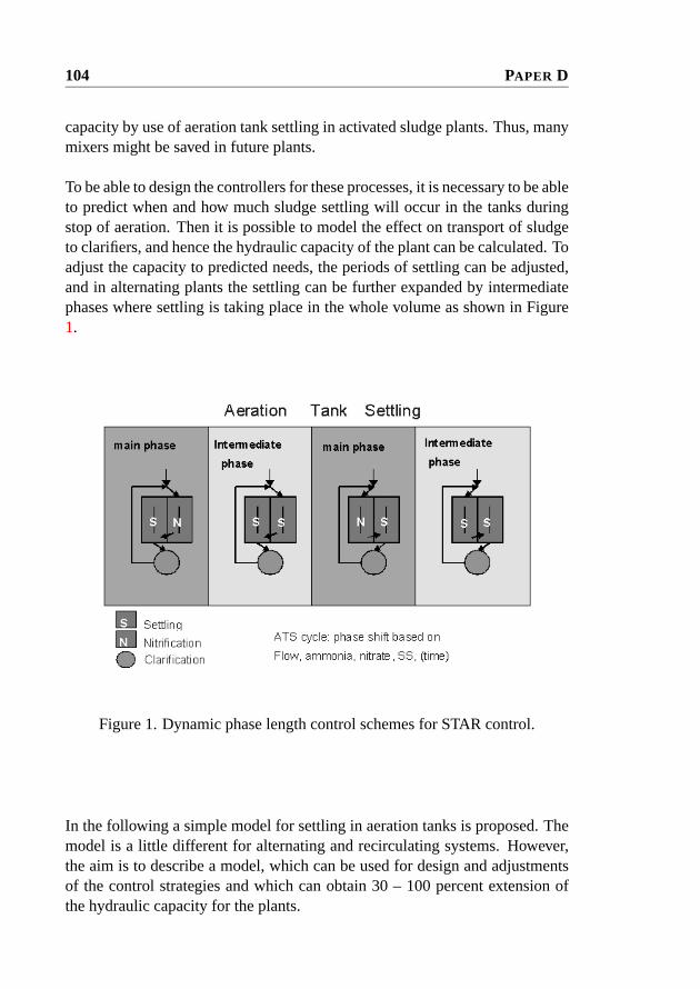
104 PAPER D
capacity by use of aeration tank settling in activated sludge plants. Thus, manymixers might be saved in future plants.
To be able to design the controllers for these processes, it is necessary to be ableto predict when and how much sludge settling will occur in the tanks duringstop of aeration. Then it is possible to model the effect on transport of sludgeto clarifiers, and hence the hydraulic capacity of the plant can be calculated. Toadjust the capacity to predicted needs, the periods of settling can be adjusted,and in alternating plants the settling can be further expanded by intermediatephases where settling is taking place in the whole volume as shown in Figure1.
Figure 1. Dynamic phase length control schemes for STAR control.
In the following a simple model for settling in aeration tanks is proposed. Themodel is a little different for alternating and recirculating systems. However,the aim is to describe a model, which can be used for design and adjustmentsof the control strategies and which can obtain 30 – 100 percent extension ofthe hydraulic capacity for the plants.

Design, Operation and Economics of Large WWTPs 105
Theory for modelling
The sludge settling starts when the turbulence in the tanks is reduced afterstopping both aeration and mixing. When the settling starts, the formula forhindered settling dependent on the mixed liquor suspended solids, MLSS, inthe interface is proposed as a two-layer model with dynamic layer heights. Theupper layer is assumed to be clear water while the lower layer is assumed tocontain all the initial sludge content which concentrates as the sludge layerheight decreases during the settling period.
The settling rate model for sludge proposed byVesilind (1979) and quantifiedby Härtel and Pöpel(1992) is used:
vSS = vS,0e−nvSS (1)
where:
vSS andvS,0 are the actual and the unhindered settling rate of sludge particles,respectively, andnv is an empiric concentration effect factor.
The modelling of the sludge blanket depth,dSB, can be done by integration ofthe settling rate over time:
dSB =∫ t
t0
vSSdt (2)
The relevant sludge concentration starts at the MLSS value in the aerated tankand increases during the settling as sludge concentrates towards the bottom.
The starting timet0 is when the turbulence is reduced.
To predict the outlet SS from the tanks in non-ideal full-scale plants the detailsof the inlet, outlet and tank geometrical design must be included in the model.
As a first simple model for SS in the top weir outlet of the aeration tank andinlet to the clarifier,SS out, can be made as a calculation of suction depth,dsuct.

106 PAPER D
��� ��������� �������
� ������� ������
��� �������� ������
�����
�������! #" $&%('()+*," -/.,0�)213%,)/41657�8:9<;�=?>!@#A&B�C6D E<FHG(I<J�CLK
M<N�O/P&Q
Figure 2. Parameter definition for modelling effluent SS.
The suction depth is predicted for the specific outlet and the concentration ismodelled as:
SS out =dsuct− dSB
dsuctSS bl (3)
Of course, the suction depth is varying with the flow rate, and the distribution ofthe actual flow is not proportional with the depth. These unmeasurable factorsare modelled by data fitting to full-scale measurements.
Physical model
Alternating systems
In the alternating system typically two tanks are available. As a rule only thelast tank before the clarifier is relevant for settling. The inlet will normally befrom an adjoining tank as seen in Figure3, and the inlet velocity and distribu-tion is of paramount importance for the efficiency of the settling as well as theoutlet distribution as it is in other clarifier designs.

Design, Operation and Economics of Large WWTPs 107
������� �����
����� ������
� ������� � ���
������������� ���
Figure 3. Physical description of outlet modelling in settling aeration tanks inan alternating plant.
Apart from simple ideal settling the model must include the reduced efficiencyof the aeration tank as clarifier because inlet and outlet is not optimal. Furtherthe storage of sludge on the bottom will limit the capacity for settling aftersome time in the same phase, as there is no sludge removal from the aerationtanks during the phases.
The inlet turbulence must be adequate enough to distribute the incoming wa-ter sufficiently in the tank under settling operation to avoid short-circuiting.For the modelling, the limitation in settling efficiency is simplest described byreducing the efficient volume of the aeration settling tank.
The outlet is more important for the time distribution of the aeration tank effi-ciency for settling. The outlet is assumed to be via a weir, and the suction depthis a function of outflow. As shown in Figure2 the concentration of sludge inthe outlet is dependent on the sludge blanket level and the SS concentrationunder the sludge blanket that is sucked out in the effluent from the tank.
The sludge build-up and concentration profile on the bottom is modelled asa single layer model, but to be able to fit the model to practical experimentsa virtual bottom is assumed, and the sludge concentration below the sludge

108 PAPER D
blanket and the virtual bottom is assumed homogeneous.
With these assumptions we have a simple model for the concentration out ofan aeration tank at any time dependent on present and previous load and on theperiod since the settling started as shown in Figure7.
Recirculating plants
In recirculating plants the settling can take place in the effluent part of theaeration tank. Apart from the stopping of the aerators in intervals, the prioritycan be to stop the effluent end aeration grids as shown in Figure4 to obtainsettling in the outlet end. The return of sludge can use the existing recirculationsystem.
��� ������� �����
�������� �����
��������� �!"!
Figure 4. Physical description of outlet modelling in a recirculating plant.

Design, Operation and Economics of Large WWTPs 109
Plant capacity
The capacity of the clarifiers is often the limiting factor during rain events.In stationary situations, the capacity of the clarifiers, according to normal de-sign rules (like the ATV rules), is inverse proportional to the sludge volumeindex,SVI , and the concentration of suspended solids,SS . Billmeier (1986)describes the steady state hydraulic capacity of the clarifiers as
Q =Vclarifier
SS outSVI k=
K
SS out(4)
wherek is a proportionality factor, specific for a given plant design, and
K =Vclarifier
SVI k(5)
is a plant specific value for a given sludge quality.
Hence, at a plant with a given clarifier volume and sludge volume index, thehydraulic capacity of the plant is inverse proportional to the suspended solidconcentration out of the aeration tank as shown above.
By introducing the aeration tank settling (ATS) operation before and duringrain, the necessary clarifier volume is reduced as illustrated in Figure5 takenfrom Nielsen et al.(1996).
Practical test
To test the model, the data from a full-scale application at Aalborg East WWTPshown in Figure6 are used.
At present this configuration is used on 3 alternating plants serving approx700.000 pe in Scandinavia. At minor rain events the model and reality look

110 PAPER D
������������ ����������� ������������ ����
�������������� ����
"!
"!
#�$ "!
% $ "!
&�'(*)
(�'(�)
+-,.0/214353
68759;:�6
6=<>9<?6
@BADC"E�FHG5G
IJADC"E2F4G5G
Figure 5. Required settler volume for two control control schemes (Nielsenet al., 1996).

Design, Operation and Economics of Large WWTPs 111
������������� �������������� �������������
������
� ����� ������ �������
���������� ���"!#��$����%�����
&�' &�'
&�'
&)(+*
,
--
.0/21�35456�75896�8:3<;�=>893?.A@CB�3ADE>FG@5DH6�8
IKJ�FLFG;�79>@L@�758M7�>DEN"@5DH6
O/2=1589PQ6SR9=@�7�TU6�D
VCWXY;�354�X5@�DH6
Z\[ 1�N�R�>8Q>D^]
_`B�@�a�1�=>3Y@�DE>;�7bDH@Q7QT
c�d
egffhikjmlkn
egffohipjmlqn
r l�fohipjmlqn
st
t
u u
Figure 6. Description of the Aalborg East alternating WWTP.

112 PAPER D
as shown in Figure7 below. Compared to conventional extension of clarifiervolume, the use of control to extend the capacity can be achieved by typically1/10 of the cost.
Figure 7. Measured and modelled MLSS out of the aeration tanks.
The modelled and measured MLSS out of aeration tanks during storm eventswith settling in the aeration tanks are shown in Figure7.
As it can be seen the modelled MLSS is nearly 45 minutes ahead of measuredvalues. This is due to delay from: 1) SCADA system, 2) Rotation in horizontalchannels and 3) delay from stop of micro-turbulence after stop of aeration andmixers, all of which are not included in the model.
Equal results are experienced from other alternating plants. Control has beenintroduced on a recirculating system at the Sydkysten WWTP, but they havenot been documented on-line yet. However, it has been experienced that thereturn sludge flow must be reduced proportionally by the length of the aeratorstop periods to maintain constant concentration in return sludge (Nielsen andÖnnerth, 1995), so a significant but smaller effect will be obtained.
Discussion
It is seen that the proposed model is qualitatively correct. Its quantification issufficient for most control, however there are some empirical constants, whichare only adjustable from practical fitting based on on-line data. Although these

Design, Operation and Economics of Large WWTPs 113
constants are explained above, as having a physical meaning, they are onlyfound from data fitting to experiences during rain events.
However, experiences show that the model can be transferred from one plant toanother. Only small adjustments, and update to actual MLSS concentration andSVI is needed, hence practical experiences from one plant can be transferredto another similar plant, and the on-line update can be obtained from the firstrain event experiences.
By use of the model and the prediction of flow from rain gauges or sewersystem it is possible to predict the needed efficiency of the ATS control andoptimize the organic versus hydraulic capacity of the plant.
Conclusion
Aeration tank settling is a robust and reliable technique, which by use of mo-dels can be designed and controlled to perform efficiently, in alternating plantsto increase their hydraulic capacity with 30 - 100% within a few hours.
The use of the same model methodology can predict the hydraulic capacityfor recirculating plants. When further experiences of the methodology of thesettling sludge and recirculation of the sludge are collected from full-scale, thestandard design technique will be extended to cover most plug flow and otherrecirculating activated sludge plants too.
Acknowledgements
We thank our co-operators within the EUREKA projects MUST and SIM-BIOSE from the Department of Mathematical Modelling, Department of En-vironmental Science and Engineering at the Technical University of Denmark,for their support and co-operation.

114 PAPER D

Paper E
Grey-box modelling ofaeration tank settling.
Submitted.
E
115


SUBMITTED . 117
Abstract
A model of the concentrations of suspended solids (SS) in the aeration tanksand in the effluent from these during Aeration Tank Settling (ATS) operationis established. The model is based on simple SS mass balances, a model of thesludge settling and a simple model of how the SS concentration in the effluentfrom the aeration tanks depends on the actual concentrations in the tanks andthe sludge blanket depth.
The model is formulated in continuous time by means of stochastic differentialequations with discrete-time observations. The parameters of the model areestimated using a maximum likelihood method from data from an alternatingBioDenipho wastewater treatment plant (WWTP).
The model is an important tool for analyzing ATS operation and for selectingthe appropriate control actions during ATS, as the model can be used to predictthe SS amounts in the aeration tanks as well as in the effluent from the aerationtanks.
Key words: Aeration Tank Settling, mass balance, grey-box models, statisticalidentification, on-line measurements.
Introduction
With the introduction of advanced optimising control systems at wastewatertreatment plants (Nielsen and Önnerth, 1995; Önnerth and Bechmann, 1995)the demand for mathematical models of the important processes in wastewa-ter treatment plants is increased. The Aeration Tank Settling (ATS) principleintroduces settling periods in aeration tanks of alternating plants and enablesincreased amounts of suspended solids (SS) to be stored in the aeration tanksduring rain storms. ATS increases the hydraulic capacity of the WWTP, butcomplicates the prediction of the SS concentration in the effluent from the ae-ration tanks, compared to dry weather operation. During dry weather operationthe aeration tanks are fully mixed, and the SS concentrations in the effluent areequal to the SS concentrations in the tanks, but during ATS operation the ef-fluent comes from an aeration tank where the sludge settles. Hence, the SS
118 PAPER E
concentrations in and out of the aeration tanks are not equal during ATS ope-ration.
To minimize the amounts of SS in the effluent, predictive models of the SSconcentrations are needed. InNielsen et al.(1999), a model of SS in the aera-tion tanks and in the effluent from these is proposed. The model consists of 3submodels: 1) A simple mass balance model for the SS concentrations in theaeration tanks, 2) a sludge settling model and 3) a model for the SS concentra-tion in the effluent from the aeration tanks. Here, the model is reformulated bymeans of stochastic differential equations, and the parameters are estimated bya maximum likelihood method.
Vesilind(1968, 1979) proposed a sludge settling velocity model of exponentialform. During recent years, several refinements to the original model have beenproposed, see e.g.Grijspeerdt et al.(1995); Dupont and Dahl(1995); Ekamaet al. (1997). In the proposed models several layers in the settling tank areincorporated to permit the calculation of SS profiles over the tank depth andpredict the SS concentrations in the return sludge and in the effluent from theclarifier.
Here, the original Vesilind model combined with a simple suction depth modelis used to enable prediction of the SS concentration in the effluent from theaeration tank. In order to make the model applicable for real time controlpurposes, only two layers of variable height in the aeration tank are considered.
Dry weather and ATS operation
In an alternating WWTP, the aeration tanks are composed of pairs of inter-connected tanks. The wastewater is directed to one of the tanks, through theconnection between the tanks and out of the second tank. In dry weather si-tuations the tanks are fully mixed to enable optimal nutrient removal. Theincoming wastewater is directed to an aeration tank with anoxic conditions,and thus with denitrification. The other tank from which the effluent is takenis aerated and is hence a tank with nitrification. Depending on the state of theprocesses in the aeration tanks, the flow path is changed.
During rain storms ATS operation is activated. When the WWTP is in ATS
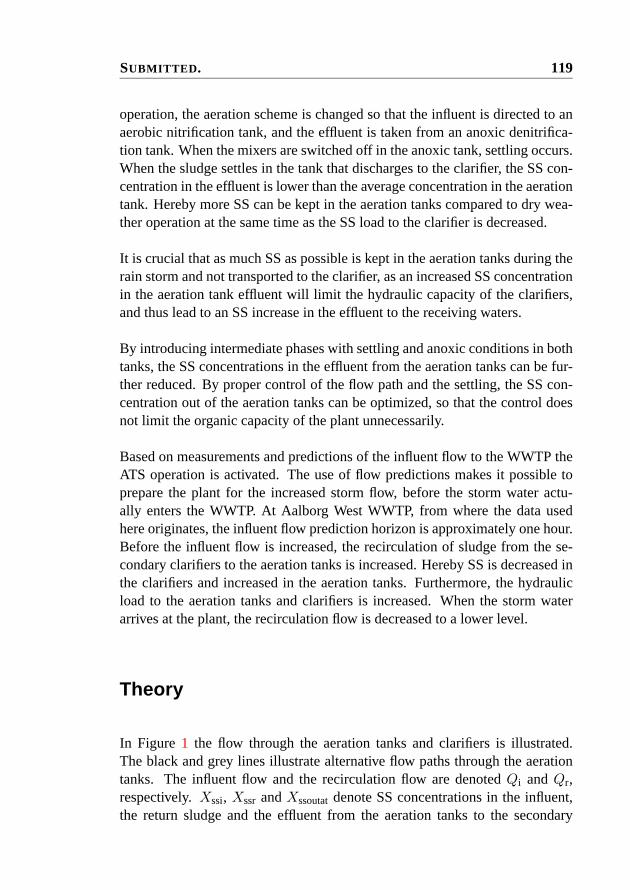
SUBMITTED . 119
operation, the aeration scheme is changed so that the influent is directed to anaerobic nitrification tank, and the effluent is taken from an anoxic denitrifica-tion tank. When the mixers are switched off in the anoxic tank, settling occurs.When the sludge settles in the tank that discharges to the clarifier, the SS con-centration in the effluent is lower than the average concentration in the aerationtank. Hereby more SS can be kept in the aeration tanks compared to dry wea-ther operation at the same time as the SS load to the clarifier is decreased.
It is crucial that as much SS as possible is kept in the aeration tanks during therain storm and not transported to the clarifier, as an increased SS concentrationin the aeration tank effluent will limit the hydraulic capacity of the clarifiers,and thus lead to an SS increase in the effluent to the receiving waters.
By introducing intermediate phases with settling and anoxic conditions in bothtanks, the SS concentrations in the effluent from the aeration tanks can be fur-ther reduced. By proper control of the flow path and the settling, the SS con-centration out of the aeration tanks can be optimized, so that the control doesnot limit the organic capacity of the plant unnecessarily.
Based on measurements and predictions of the influent flow to the WWTP theATS operation is activated. The use of flow predictions makes it possible toprepare the plant for the increased storm flow, before the storm water actu-ally enters the WWTP. At Aalborg West WWTP, from where the data usedhere originates, the influent flow prediction horizon is approximately one hour.Before the influent flow is increased, the recirculation of sludge from the se-condary clarifiers to the aeration tanks is increased. Hereby SS is decreased inthe clarifiers and increased in the aeration tanks. Furthermore, the hydraulicload to the aeration tanks and clarifiers is increased. When the storm waterarrives at the plant, the recirculation flow is decreased to a lower level.
Theory
In Figure 1 the flow through the aeration tanks and clarifiers is illustrated.The black and grey lines illustrate alternative flow paths through the aerationtanks. The influent flow and the recirculation flow are denotedQi andQr,respectively.Xssi, Xssr andXssoutatdenote SS concentrations in the influent,the return sludge and the effluent from the aeration tanks to the secondary

120 PAPER E
Aer
atio
n ta
nk p
air
AT
2
AT
1
iQ
iQ
Qr
Qr,
Xss
r
Seco
ndar
y cl
arif
ier
Inco
min
gw
aste
wat
er
Ret
urn
slud
ge
, X
ssi
+X
ssou
tat
Exc
ess
slud
ge
wQ
, X
ssrw
ater
sT
o re
ceiv
ing
Figure 1. Flow path through aeration tank pair in an alternating WWTP.

SUBMITTED . 121
clarifers. The dynamics of the water amounts in the aerations tanks are notconsidered, i.e. it is assumed that the flows to and from each of the aerationtanks are the same (Qi + Qr). Furthermore, the SS concentration in the flowbetween the two aeration tanks is assumed to be the average SS concentrationin the feeding tank. When the feeding tank is fully mixed, this assumption isfulfilled, but when settling occurs it is an approximation.
The mass balance equations for each of the aeration tanks depend on the actualflow path designatedfp. Whenfp = 1 the influent flow is directed to aerationtank 1, and the effluent flow is taken from tank 2.fp is 0 when the oppositeflow path is applied. WithVat, Xssm1andXssm2denoting the volume of eachof the equally sized aeration tanks and the average SS concentrations in tank 1and 2, respectively, the mass balance equations can be established.
Forfp = 1 the mass balance equations for the aeration tanks are:
dXssm1
dt=QiXssi +QrXssr− (Qi +Qr)Xssm1
Vat(1)
dXssm2
dt=
(Qi +Qr)Xssm1− (Qi +Qr)Xssoutat
Vat(2)
Forfp = 0 the mass balance equations are:
dXssm1
dt=
(Qi +Qr)Xssm2− (Qi +Qr)Xssoutat
Vat(3)
dXssm2
dt=
(QiXssi +QrXssr)− (Qi +Qr)Xssm2
Vat(4)
The flow path variable can be used to combine equation (1) with (3) and equa-tion (2) with (4) into one equation per aeration tank:
dXssm1
dt= fp
QiXssi +QrXssr− (Qi +Qr)Xssm1
Vat
+ (1− fp)(Qi +Qr)Xssm2− (Qi +Qr)Xssoutat
Vat
(5)
and:
dXssm2
dt= fp
(Qi +Qr)Xssm1− (Qi +Qr)Xssoutat
Vat
+ (1− fp)(QiXssi +QrXssr)− (Qb +Qr)Xssm2
Vat
(6)

122 PAPER E
atd
atd dsb
dat
dsb
- ssmXX =X = ssslss
ssX = 0
Figure 2. Two layer model of settling in an aeration tank.
When mixing is stopped in an aeration tank, the suspended solids settle. Asimple two layer model, where the water in the layer above the sludge blanketis assumed to be clear water, and the layer under the sludge blanket is assumedto contain all the SS fully mixed, is used. The settling velocity for the sludgeblanket is modelled according toVesilind (1968) as:
ddsb
dt= V0 e−nvXsssl (7)
wheredsb andXsssl denote the sludge blanket depth and the SS concentrationin the sludge layer, respectively, see Figure2, andV0 andnv are sludge vol-ume index (SVI ) dependent parameters. For simplicity we use the expressionsfound byHärtel and Pöpel(1992):
V0 = (17.4 e−0.0113SVI +3.931)mh
nv = (−0.9834 e−0.00581SVI +1.043)lg
(8)
If sludge blanket depth measurements are available,V0 andnv can be estima-ted.
As the volume of the sludge layer is(dat− dsb)Vat/dat, the average SS concen-tration in the sludge layer is:
Xsssl =dat
dat− dsbXssm (9)
whereXssm is the average SS concentration in the aeration tank.
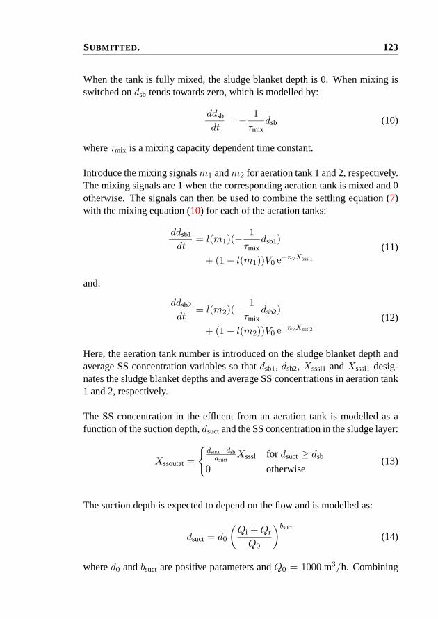
SUBMITTED . 123
When the tank is fully mixed, the sludge blanket depth is 0. When mixing isswitched ondsb tends towards zero, which is modelled by:
ddsb
dt= − 1
τmixdsb (10)
whereτmix is a mixing capacity dependent time constant.
Introduce the mixing signalsm1 andm2 for aeration tank 1 and 2, respectively.The mixing signals are 1 when the corresponding aeration tank is mixed and 0otherwise. The signals can then be used to combine the settling equation (7)with the mixing equation (10) for each of the aeration tanks:
ddsb1
dt= l(m1)(− 1
τmixdsb1)
+ (1− l(m1))V0 e−nvXsssl1
(11)
and:
ddsb2
dt= l(m2)(− 1
τmixdsb2)
+ (1− l(m2))V0 e−nvXsssl2
(12)
Here, the aeration tank number is introduced on the sludge blanket depth andaverage SS concentration variables so thatdsb1, dsb2, Xsssl1andXsssl1desig-nates the sludge blanket depths and average SS concentrations in aeration tank1 and 2, respectively.
The SS concentration in the effluent from an aeration tank is modelled as afunction of the suction depth,dsuctand the SS concentration in the sludge layer:
Xssoutat=
{dsuct−dsbdsuct
Xsssl for dsuct≥ dsb
0 otherwise(13)
The suction depth is expected to depend on the flow and is modelled as:
dsuct = d0
(Qi +Qr
Q0
)bsuct
(14)
whered0 andbsuct are positive parameters andQ0 = 1000 m3/h. Combining
124 PAPER E
0
0.1
0.2
0.3
0.4
0.5
0.6
0.7
0.8
0.9
1
-5 -4 -3 -2 -1 0 1 2 3 4 5
b=0.2b=1.0b=2.0
Figure 3. The logistic function fora = 0 and differentb values.
(9) and (13) yields
Xssoutat=dsuct− dsb
dsuct
dat
dat− dsbXssm
=1− dsb/dsuct
1− dsb/datXssm for dsuct> dsb
(15)
To enable smooth changes inXssoutatwhen the pointdsuct = dsb is passed asmooth threshold function is introduced. Here, the logistic function:
l(x) = l(x, a, b) =1
1 + ea−xb
(16)
is used. Forx = a the logistic function is 0.5, i.e. the value ofa determines themidpoint of the switch between 0 and 1. By appropriate selection ofa andb thechange between 0 and 1 ofl(x, a, b) can be controlled. In Figure3 the logisticfunction is shown fora = 0 and 3 different values ofb. In the followingb > 0is assumed.
The logistic function (16) is used to calculateXssoutatwhile the flow path vari-
SUBMITTED . 125
able is used select the discharge tank:
Xssoutat= fp
(l(dsuct− dsb2)
1− dsb2/dsuct
1− dsb2/datXssm2
)(1− fp)
(l(dsuct− dsb1)
1− dsb1/dsuct
1− dsb1/datXssm1
) (17)
As dsuct is only dependent on the flow, there is no need to consider differentsuction depths for each of the aeration tanks.
In order to use a matrix notation, introduce the state vectorX, the input vectorU and the observation vectorY :
X = [Xssm1, Xssm2, dsb1, dsb2]′
U = [fp,m1,m2, Xssr, Qi , Qr]′
Y = [Xssm2, Xssoutat]′(18)
Here, it is assumed that aeration tank 2 is equipped with a suspended solidssensor.
By use of the vector functionf(X,U , t) the mass balances and sludge blanketdepth equations can be expressed in a vector differential equation:
dX(t)dt
= f(X,U , t) (19)
wheref(X,U , t) is easily constructed from equations (5)–(12) and (18).
The measurements are described by the observation equation
Y (t) = h(X,U , t) (20)
whereh(X,U , t) is constructed from equations (17) and (18).
To count in uncertainties in the model formulation and to enable use of themaximum likelihood parameter estimation method, stochastic noise terms areintroduced. Hence, equation (19) turns into a stochastic differential equation,where the continuous time equations describing the mass balances and thesludge blanket depths in the aeration tanks can be written as the so-called Itôdifferential equation (Øksendal, 1995):
dX(t) = f(X,U , t) dt+G(X,U , t) dw(t) (21)

126 PAPER E
where the stochastic processw(t) is assumed to be a standard vector Wienerprocess (see e.g.Kloeden and Platen(1995)). The functionG(X,U , t) de-scribes any state, input or time dependent variation related to how the variationgenerated by the Wiener process enters the system.
Here,G is assumed to be a constant diagonal matrix:
G(X,U , t) = G =
σss 0 0 00 σss 0 00 0 σsb 00 0 0 σsb
(22)
Hereby, the covariance ofG dw(t) becomes
Σ = GG′ =
σ2
ss 0 0 00 σ2
ss 0 00 0 σ2
sb 00 0 0 σ2
sb
(23)
The observation uncertainties are included in the observation equation:
Y (t) = h(X,U , t) + e(t) (24)
where the terme(t) is the measurement error, which is assumed to be a zeromean Gaussian white noise sequence independent ofw(t) and with covariancematrix:
V (e(t)) =[σ2
ss2(t) 00 σ2
ssoutat(t)
](25)
Estimation method
The method used to estimate the parameters of the model (21)–(22) and (24)is a maximum likelihood method for estimating parameters in stochastic diffe-rential equations based on discrete-time data given by (24). For a more detaileddescription of the method refer toMadsen and Melgaard(1991) or Melgaardand Madsen(1993).
All the unknown parameters, denoted by the vectorθ, are embedded in thecontinuous-discrete time state space model (21) and (24).

SUBMITTED . 127
The measurements are given in discrete time, and, in order to simplify thenotation, it is assumed that the time indext belongs to the set{0, 1, 2, ..., N},whereN is the number of observations. Introducing
Y(t) = [Y (t),Y (t− 1), . . . ,Y (1),Y (0)]′ (26)
i.e. Y(t) is a vector containing all the observations up to and including timet, the likelihood function is the joint probability density of all the observationsassuming that the parameters are known, i.e.
L′(θ;Y(N)) = p(Y(N)|θ)= p(Y (N)|Y(N − 1),θ)p(Y(N − 1)|θ)
=( N∏t=1
p(Y (t)|Y(t− 1),θ))p(Y (0)|θ)
(27)
where successive applications of the ruleP (A∩B) = P (A|B)P (B) are usedto express the likelihood function as a product of conditional densities.
In order to evaluate the likelihood function it is assumed that all the conditio-nal densities are Gaussian. In the case of a linear state space model, it is easilyshown that the conditional densities actually are Gaussian (Madsen and Mel-gaard, 1991). In the more general non-linear case, as described by (21) and(24), the Gaussian assumption is an approximation.
The Gaussian distribution is completely characterized by the mean and covari-ance. Hence, in order to parameterize the conditional densities in (27), weintroduce the conditional mean and the conditional covariance as
Y (t|t− 1) = E[Y (t)|Y(t− 1),θ] and
R(t|t− 1) = V [Y (t)|Y(t− 1),θ](28)
respectively. It should be noted that these correspond to the one-step predictionand the associated covariance, respectively. Furthermore, it is convenient tointroduce the one-step prediction error (or innovation)
ε(t) = Y (t)− Y (t|t− 1) (29)
For calculating the one-step prediction and its variance, an iterated extendedKalman filter is used. The extended Kalman filter is simply based on a line-arization of the system equation (21) around the current estimate of the state

128 PAPER E
(seeGelb (1974)). The iterated extended Kalman filter is obtained by localiterations of the linearization over a single sample period.
Using (27) – (29) the conditional likelihood function (conditioned onY (0))becomes
L(θ;Y(N))
=N∏t=1
((2π)−m/2 detR(t|t− 1)−1/2 exp(−1
2ε(t)′R(t|t− 1)−1ε(t))
) (30)
wherem is the dimension of theY vector. Traditionally the logarithm of theconditional likelihood function is considered
logL(θ;Y(N))
= −12
N∑t=1
(log detR(t|t− 1) + ε(t)′R(t|t− 1)−1ε(t)
)+ const
(31)
The maximum likelihood estimate (ML-estimate) is the setθ, which maxi-mizes the likelihood function. Since it is not, in general, possible to optimizethe likelihood function analytically, a numerical method has to be used. Areasonable method is the quasi-Newton method.
An estimate of the uncertainty of the parameters is obtained by the fact that theML-estimator is asymptotically normally distributed with meanθ and covari-ance
D = H−1 (32)
where the matrixH is given by
{hlk} = −E[
∂2
∂θl∂θklogL(θ;Y(N))
](33)
An estimate ofD is obtained by equating the observed value with its expecta-tion and applying
{hlk} ≈ −(
∂2
∂θl∂θklogL(θ;Y(N))
)|θ=θ
(34)
The above equation can be used for estimating the variances of the parameterestimates. The variances serves as a basis for calculating t-test values for tests
SUBMITTED . 129
under the hypothesis that the parameter is equal to zero. Finally, the correla-tion between the parameter estimates is readily found based on the covariancematrixD.
Unreliable measurements are handled by adjusting the variance ofe(t). Whenan unreliable observation is encountered, the corresponding observation vari-ance is considerably increased. As the extended Kalman filter uses the ob-servation noise variance and the intensity of the Wiener process, that count forstate noise, the unreliable observations are taken into account by the estimationprocedure.
Results and discussion
Aalborg West WWTP, from where the data used for the estimations originates,has three aeration tank pairs, which are controlled in an identical way, exceptfor a time delay between the tank pairs. The master tank pair consists of aera-tion tanks 5 and 6, of which tank 6 is equipped with an SS sensor. The flowpath and mixing of tanks 3 and 4 are delayedTd = 12 min in relation to tanks5 and 6, and tank 1 and 2 are delayed furtherTd. To include all 6 aeration tanksin the model, it is extended with equations for the 4 additional tanks. The flowsto and from each tank pair are reduced to a third of the total flows, and the timedelay between the tank pairs is taken into account in the flow path and mixingsignals to the respective tank pairs. The resulting SS concentration out of theaeration tanks is the average of the SS concentrations out of the 3 tank pairs.The Aalborg West WWTP model is thus a 12 state non-linear model with 2observations,Xssm6andXssoutat.
The measurements of the average SS concentration in aeration tank 6 are onlyreliable when the tank is fully mixed. This is taken into account by adjustingthe variance ofe(t) according to the mixing of aeration tank 6. When the tankis not mixed,σ2
ss6(t) is large (ideally∞) compared to the value ofσ2ss6(t) when
the tank is mixed.
Aalborg West WWTP is equipped with a STAR (Superiour Tuning And Re-porting) control system (Nielsen and Önnerth, 1995; Önnerth and Bechmann,1995), which optimizes the operation of the plant. In the STAR system, mea-surements are fetched and control actions are computed every 6 minutes. This

130 PAPER E
turned out to be a too short sampling time for the estimation procedure, hence,the data was re-sampled to a longer sampling period. Furthermore, it turnedout that there was a significant time delay between the input variables (the flowdirection, the mixing signals and the flows and concentrations to the aerationtanks) and the output variables (SS concentrations in aeration tank 6 and outof the aeration tanks). The time delay was found to be 0.8 h, and the newsampling interval selected was 0.2 h.
The parameters of the model were estimated on one data set and the resultingmodel was cross validated on another data set. It was not possible to estimatethe sludge settling model parametersV0 andnv and the parameters of the suc-tion depth modeld0 andbsuct simultaneously. This is due to the fact that thesetwo sub-models are closely correlated, as a change in the sludge settling modelwill be compensated by an equivalent change in the suction depth model. TheSVI for the estimation data set was 142, hence the sludge settling parametersfound from (8) are
V0 = 7.43 m/h and nv = 0.612 m3/kg SS (35)
The SVI for the validation data set was 177, which gives the correspondingsludge settling parameters
V0 = 6.29 m/h and nv = 0.691m3/kg SS (36)
By inspecting the data before the estimation was carried out, systematic errorsin the SS concentration measurements were observed. As it is not possiblefrom the available measurements to detect which of the measurements thatare correct, it was decided to useXss6 as the reference. The errors on themeasurements ofXssoutatwere included in the model as offset errors, eventhough other methods could be applied. For the errors in the return sludgemeasurements both an additive and a multiplicative form were tried out. Itwas found that both types gave similar results, and the multiplicative form wasused in the final estimations. The bias onXssoutatdesignatedXssout,band thefactor onXssr designatedXssr,f were estimated simultaneously with the otherparameters.
The influent SS concentrationXssi was sought estimated as constant during theperiod considered. This parameter was, however, found to be insignificant, andtherefore excluded from the final estimation.
The estimated parameters as well as their estimated standard deviations are

SUBMITTED . 131
Par
amet
erd
0b s
uct
Xss
r,fX
ssou
t,bσ
2 ssσ
2 sbσ
2 ss6
σ2 ss
outa
t
Uni
tm
––
g/l
(g/l)
2m
2(g
/l)2
(g/l)
2
Est
imat
e1.
005
0.16
41.
129
0.14
30.
0259
1.34
1.91
10-4
1.78
10-7
Sta
ndar
dde
viat
ion
0.01
50.
022
0.00
90.
014
0.00
380.
090.
2810
-42.
0810
-7
Table 1. Maximum likelihood estimates of the parameters of the model.

132 PAPER E
shown in Table1. All the parameters exceptσ2ssoutatare estimated with small
standard deviations. The estimate ofσ2ssoutatis thus uncertain.
The measured and modelled SS concentrations are shown in Figures4 and5,for a part of the estimation data set and the validation data set, respectively.The mixing signal for aeration tank 6 is included in theXss6graphs to indicatethe validity of theXss6measurements, as these are only reliable when mixingis on. Note that the modelled SS concentrations are simulations based onlyon the input variables to the model, and not one-step ahead predictions, whichuse the measurements of the output variables at every time step to predict theoutput at the next time step.
For the validation data set theV0 andnv parameters for bothSVI = 142(the estimation data set value) andSVI = 177 (the validation data set value)were tried. The best result was obtained with the parameter values for theestimation data set, hence, these values were used to make the graphs. Thefact that the values ofV0 andnv for the estimation data set performed betterwith the validation data set indicates that the sludge settling model, the suctiondepth model and theXssoutatmodel are interdependent. These should thus beregarded as a single sub-model, and not independent sub-models. The modelis found to perform well as regards the SS concentrations in aeration tank 6for both the estimation data set and the validation data set. The simulatedSS concentrations in the effluent from the aeration tanks are not as good forthe validation data set as for the estimation data set. This indicates that thecombined model consisting of the sludge settling model, the suction depthmodel and theXssoutatmodel could be refined.
The estimation method relies on the assumption that the observation noise iswhite. The validity of this assumption is checked by use of cumulative residualperiodograms, see Figs.6 and7. As only the observations ofXss6 in aeratedperiods are reliable, the non-aerated periods result in residuals that can notbe considered to be generated by a white noise process. Hence, the cumula-tive residual periodograms are shown only for theXssoutatobservations. Theconfidence limits for the periodograms are calculated using the Kolmogorov-Smirnov test principle (Kendall and Stuart, 1979; Box and Jenkins, 1976). Asthe periodograms are between the confidence limits, theXssoutatresiduals canbe considered to be white noise. Note that the confidence band for the valida-tion data is wider than for the estimation data. This is caused by the fact thatthe estimation data set contains more observations than the validation data set.

SUBMITTED . 133
2
2.5
3
3.5
4
4.5
5
5.5
6
6.5
25 Oct ’9800:00
25 Oct ’9812:00
26 Oct ’9800:00
26 Oct ’9812:00
27 Oct ’9800:00
On
Off
Xss
m6� (
g/l)
Aer
atio
n/m
ixin
g in
AT
6
Aalborg W. WWTP, e22e-8-2
Xssm6 measuredXssm6 simulatedm6
1
1.5
2
2.5
3
3.5
4
4.5
5
25 Oct ’9800:00
25 Oct ’9812:00
26 Oct ’9800:00
26 Oct ’9812:00
27 Oct ’9800:00
Xss
outa
t (g/
l)
Aalborg W. WWTP, e22e-8-2
Xssoutat measuredXssoutat simulated
Figure 4. Measured and simulated SS concentrations in aeration tank 6 and inthe effluent from the aeration tanks, estimation data set.

134 PAPER E
3.5
4
4.5
5
5.5
6
6.5
03 Apr ’9818:00
04 Apr ’9800:00
04 Apr ’9806:00
04 Apr ’9812:00
04 Apr ’9818:00
On
Off
Xss
m6� (
g/l)
Aer
atio
n/m
ixin
g in
AT
6
Aalborg W. WWTP, v8-8-2
Xssm6 measuredXssm6 simulatedm6
2.4
2.6
2.8
3
3.2
3.4
3.6
3.8
4
4.2
4.4
03 Apr ’9818:00
04 Apr ’9800:00
04 Apr ’9806:00
04 Apr ’9812:00
04 Apr ’9818:00
Xss
outa
t (g/
l)
Aalborg W. WWTP, v8-8-2
Xssoutat measuredXssoutat simulated
Figure 5. Measured and simulated SS concentrations in aeration tank 6 and inthe effluent from the aeration tanks, validation data set.
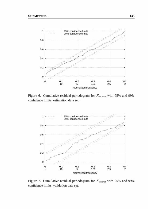
SUBMITTED . 135
0
0.2
0.4
0.6
0.8
1
0-
0.110
0.25
0.33.33
0.42.5
0.52
Normalized frequencyNormalized period
95% confidence limits99% confidence limits
Figure 6. Cumulative residual periodogram forXssoutatwith 95% and 99%confidence limits, estimation data set.
0
0.2
0.4
0.6
0.8
1
0-
0.110
0.25
0.33.33
0.42.5
0.52
Normalized frequencyNormalized period
95% confidence limits99% confidence limits
Figure 7. Cumulative residual periodogram forXssoutatwith 95% and 99%confidence limits, validation data set.

136 PAPER E
Conclusions
A model for the SS concentrations in and out of the aeration tanks in an alter-nating WWTP is proposed, and the parameters are estimated using the maxi-mum likelihood method.
The estimated model shows good agreement between simulated and measuredSS concentrations in the aeration tanks and in the effluent from these at Aal-borg West WWTP. However, improvements are still possible. The sub-modelsfor the sludge settling velocity, the suction depth and the SS concentration outof the aeration tanks are subjects for refinements, and the model should betested under conditions with more flow variation as well as at other WWTPs.Furthermore, the inclusion of the secondary clarifiers in the model is an im-portant improvement, as the objective is to keep the effluent to the receivingwaters to a minimum.
Due to time delays in the aeration tanks the model simulations are 0.8 h aheadof the measurements. Combined with an influent flow forecast horizon of ap-proximately 1 h, the SS concentrations out of the aeration tanks can be pre-dicted almost 2 h ahead. This horizon is considered to be sufficient for select-ing the optimal control action.
The proposed model is a valuable tool for designing control algorithms forATS. By applying the models, it is possible to forecast the SS concentrationin the effluent from the aeration tanks. The predictions can be used to choosethe best control action, i.e. whether to change the flow direction and switchaeration and mixing on or off, within the limitations, caused by the nutrientremoval processes.
Acknowledgements
The authors wish to thank the staff of Aalborg West WWTP and the munici-pality of Aalborg, for their cooperation and permission to use the data from theWWTP. Thanks are also due to Krüger A/S and the Danish Academy of Tech-nical Sciences for funding the project in connection with which the presentwork has been carried out, under grant EF-623.
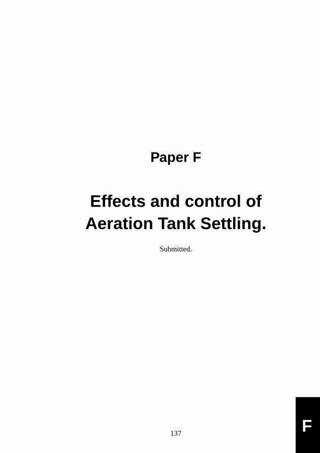
Paper F
Effects and control ofAeration Tank Settling.
Submitted.
F137

SUBMITTED . 139
Abstract
Aeration Tank Settling (ATS) operation is introduced at alternating wastewa-ter treatment plants (WWTPs) to increase the hydraulic capacity during rainstorms. A recently developed dynamic grey-box model of ATS as well as a dy-namic model of dry weather operation is used to quantify the benefits of ATSoperation in terms of increased hydraulic capacity on a large Danish alternatingBio Denipho WWTP.
A real time control algorithm for optimal selection of operating mode based onmodel predictions of the SS concentrations in the aeration tanks is proposed.
The economic value of ATS operation is estimated by a calculation of the priceof a detention basin capable of handling nearly the same amount of water asthe increased hydraulic capacity entails.
Key words: Aeration Tank Settling, model based predictive control, grey-boxmodels
Introduction
In an alternating wastewater treatment plant (WWTP) the aeration tanks arecomposed of pairs of interconnected tanks. The influent to the aeration tanksis directed to one of the tanks, through the connection between the tanks andout of the second tank to the secondary clarifier. During dry weather peri-ods, the tanks are always fully mixed to enable optimal nutrient removal. Thetank which receives the incoming wastewater is in anoxic denitrification mode,while the other tank, which delivers effluent to the secondary clarifier, is oper-ated in aerobic nitrification mode.
During rain storms, the wet weather flow often exceeds the capacity of theclarifier, and the usual approach to this situation is to store the excess waterin detention basins and/or bypass the biological treatment part of the WWTP.Another approach is to handle the excess water in the biological part of theWWTP by increasing the secondary clarifier volume, e.g. by using availablestorm water tanks for sedimentation (Carrette et al., 1999). Yet another way to

140 PAPER F
Aer
atio
n ta
nk p
air
AT
2
AT
1
iQ
iQ
Qr
Qr,
Xss
r
Seco
ndar
y cl
arif
ier
Inco
min
gw
aste
wat
er
Ret
urn
slud
ge
, X
ssi
+X
ssou
tat
Exc
ess
slud
ge
wQ
, X
ssrw
ater
sT
o re
ceiv
ing
Figure 1. Flow path through aeration tank pair in an alternating WWTP.

SUBMITTED . 141
increase the hydraulic capacity of the biological treatment during rain stormsis to introduce aeration tank settling (ATS) operation1 (Bundgaard et al., 1996;Nielsen et al., 1996, 1999).
When ATS is active, the aeration scheme is changed, so that the aeration tankthat receives influent is aerated and the other tank not. By stopping the mixersin the non aerated tank, sludge settling is made possible, which enables anincreased amount of SS to be held in the aeration tanks. Hereby, the SS loadto the secondary clarifier can be reduced, and hence the hydraulic capacityincreased. The effect of ATS can be increased by introducing an intermediatephase with settling periods in the tank that receives influent, to start the sludgesettling before the flow path is switched. ATS operation thus consists of thefour phases illustrated in Figure2.
The benefits of ATS are better wastewater treatment during wet weather pe-riods and economics compared to building storm water tanks (Boonen et al.,1999).
When a rain storm can be predicted ahead of the arrival of the storm waterat the WWTP, the prediction horizon can be used to transport SS from thesecondary clarifer to the aeration tanks, and hereby further increase the effectof ATS control.
The selection of the lengths of the periods with aeration in one of the tanks(main phases) and the periods with no aeration at all (intermediate phases) du-ring ATS is a trade off between two objectives: 1) to keep as much suspendedsolids in the aeration tanks as possible, and 2) to obtain optimal aeration capa-city. Long main and intermediate phase lengths fulfil the first objective, whileshorter main phases and no intermediate phases satisfy the second objective.Hence, it is important to choose the phase lengths to ensure that the neededhydraulic capacity is available with minimum limitation of aeration capacity.To utilize the available hydraulic capacity of a given plant with given sludgecharacteristics and sludge amounts, the sludge storage capacity of the clarifiermust be used. It is assumed that the sludge storage capacity can be quantifiedin terms of how much sludge from the aeration tanks that can be stored in theclarifier without limiting the hydraulic capacity.
1ATS is patented by Krüger A/S
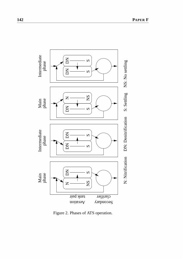
142 PAPER F
NS
NS
phas
eph
ase
Inte
rmed
iate
phas
eph
ase
Inte
rmed
iate
Mai
nM
ain S
SS
SS
S
NN
DN
DN
DN
DN
DN
DN
Aerationtank pair
Secondaryclarifier
N: N
itrif
icat
ion
D
N: D
enitr
ific
atio
n
S: S
ettli
ng
NS:
No
settl
ing
Figure 2. Phases of ATS operation.
SUBMITTED . 143
Theory
A grey-box model of the suspended solids (SS) concentrations in and out ofthe aeration tanks of an alternating WWTP during ATS operation has recentlybeen developed (Bechmann et al., 1999c; Nielsen et al., 1999). The modelconsists of 3 submodels: 1) A simple mass balance for the SS concentrationsin the aeration tanks, 2) a sludge settling model, and 3) a model for the SSconcentration in the effluent from the aeration tanks.
In Figure1 an aeration tank pair composed of the aeration tanks AT1 and AT2as well as the secondary clarifier is illustrated. The mean SS concentrationsin AT1 and AT2 are designatedXssm1andXssm2, whileXssi, XssoutatandXssr
denote the SS concentrations in the incoming wastewater, in the effluent fromthe aeration tanks to the secondary clarifer, and in the return sludge flow, re-spectively.Qi , Qr, andQw, denote the incoming wastewater flow, the returnsludge flow and the excess sludge flow, respectively.
When the incoming wastewater is directed to AT1, and the effluent is takenfrom AT2, the mass balance equations are:
dXssm1
dt=QiXssi +QrXssr− (Qi +Qr)Xssm1
Vat(1)
dXssm2
dt=
(Qi +Qr)Xssm1− (Qi +Qr)Xssoutat
Vat(2)
whereVat is the volume of each of the equally sized aeration tanks.
For the opposite flow direction, the mass balance equations are
dXssm1
dt=
(Qi +Qr)Xssm2− (Qi +Qr)Xssoutat
Vat(3)
dXssm2
dt=
(QiXssi +QrXssr)− (Qb +Qr)Xssm2
Vat(4)
The sludge settling in an aeration tank is modelled by a simple two layer model,where the layer above the sludge blanket is assumed to be clear water, and thelayer under the sludge blanket contains all the SS fully mixed, see Figure3.The sludge blanket settling velocity is modelled according toVesilind (1968):
ddsb
dt= V0 e−nvXsssl (5)
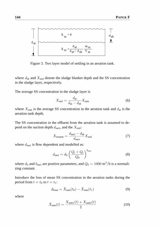
144 PAPER F
X = 0ss
atd
atd dsb
dat
dsb
ssX =ssm
V at-
Figure 3. Two layer model of settling in an aeration tank.
wheredsb andXsssl denote the sludge blanket depth and the SS concentrationin the sludge layer, respectively.
The average SS concentration in the sludge layer is
Xsssl =dat
dat− dsbXssm (6)
whereXssm is the average SS concentration in the aeration tank anddat is theaeration tank depth.
The SS concentration in the effluent from the aeration tank is assumed to de-pend on the suction depthdsuct, and theXsssl:
Xssoutat=dsuct− dsb
dsuctXsssl (7)
wheredsuct is flow dependent and modelled as:
dsuct = d0
(Qi +Qr
Q0
)bsuct
(8)
whered0 andbsuct are positive parameters, andQ0 = 1000 m3/h is a normali-zing constant.
Introduce the loss of mean SS concentration in the aeration tanks during theperiod fromt = t0 to t = t1:
∆ssat= Xssm(t0)− Xssm(t1) (9)
where
Xssm(t) =Xssm1(t) +Xssm2(t)
2(10)

SUBMITTED . 145
is the average SS concentration in the aeration tanks at timet.
When it is assumed that the SS amounts that enter the aeration tanks fromthe influent and that come from sludge growth are equal to the SS amountsremoved from the system with the excess sludge and with the effluent to therecepient, the increase in the SS concentration in the secondary clarifier is:
∆sssc=Vat
Vsc∆ssat (11)
whereVat andVsc denote the total volume of the aeration tanks and the secon-dary clarifer, respectively.
From (11) it can be seen that∆ssatis a measure of the increase of SS in the se-condary clarifier. At a given operating point (return sludge flow, effluent flow,sludge characteristcs etc.) the secondary clarifier is only capable of handling alimited increase of SS, before the SS concentration in the effluent to the receiv-ing waters is increased to an unacceptable level. Hence,∆ssatmust be limitedto a certain level, dependent on the WWTP considered and its operational state.
Dry weather operation
During dry weather operation the aeration tanks are fully mixed, hence,Xssoutat
= Xssm2when the effluent is taken from aeration tank 2, andXssoutat= Xssm1
when the opposite flow path is used. Thus, when the wastewater is directed toaeration tank 1 and effluent is taken from aeration tank 2, the dry weather massbalance equations are
dXssm1
dt=QiXssi +QrXssr− (Qi +Qr)Xssm1
Vat(12)
dXssm2
dt=
(Qi +Qr)Xssm1− (Qi +Qr)Xssm2
Vat(13)
Note that the mass balance equations for AT1 during ATS operation (equation(1)) and during dry weather operation (equation (12)) are the same, but that thecorresponding equations for AT2 (equations (2) and (13)) are not the same.
When it is assumed that the SS concentrations in the two aeration tanks as well

146 PAPER F
as their time derivatives are approximately equal, ie:
Xssm = Xssm1= Xssm2 (14)
dXssm
dt=
dXssm1
dt=
dXssm2
dt(15)
the addition of (12) and (13) yields
dXssm
dt=QiXssi +QrXssr− (Qi +Qr)Xssm
2Vat(16)
which for constantQi ,Qr,Xssi,Xssr andVat has the solution
Xssm(t) =QiXssi +QrXssr
Qi +Qr
(1− e−
Qi+Qr2Vat
(t−t0))
+Xssm(t0) e−Qi+Qr
2Vat(t−t0)
(17)
Hence, the loss of SS concentration in the aeration tanks during dry weatheroperation during the period fromt = t0 to t = t1 is
∆ssat= Xssm(t0)−Xssm(t1)
=(Xssm(t0)− QiXssi +QrXssr
Qi +Qr
)(1− e−
Qi+Qr2Vat
(t1−t0))
(18)
The steady state solution to (16) is easily found to be
Xssm,ss=QiXssi +QrXssr
Qi +Qr(19)
with the corresponding SS concentration loss
∆ssat= Xssm(t0)− QiXssi +QrXssr
Qi +Qr(20)
Choice of operating mode
During a storm situation the main objective is to avoid sludge flight to the re-cepient, and the secondary objective is to enable optimal biological treatmentof the incoming wastewater. Hence, the operating mode that prevents unac-ceptable SS concentrations in the effluent and enables best possible biological
SUBMITTED . 147
treatment should be chosen. This choice can be made on the basis of pre-dictions of the loss of SS concentration in the aeration tanks for the possibleoperating modes. The model of ATS operation can be used to predict the lossby simulation for a sufficient time to reach steady state conditions, while equa-tion (20) is used to predict the dry weather operation loss. When the acceptableloss for the WWTP considered is known, e.g. from experience from previousrain storms, the optimal operating mode can be selected. As the SS concen-tration loss predictions can be computed offline for different combinations offlows, concentrations and operating modes, the real time control algorithm canbe established by feedback fromQi ,Qr,Xssr and the initial SS concentrationsin the aeration tanks, e.g. implemented in a look-up table.
Results and discussion
The Aalborg West WWTP in Northern Jutland, Denmark, was used to estimatethe model for the ATS operation (Bechmann et al., 1999c), and hence it is usedfor the analyses carried out here.
The maximum loss of average SS concentration in the aeration tanks duringdry weather operation as well as ATS operation was calculated for varyingflowsQi andQr, varying return sludge concentrationsXssr and varying initialaverage concentrations in the aeration tanks. The simulations of ATS operationwere run for a time span of approximately 24 hours in order to enable the ATSoperation to reach steady state conditions.
In Bechmann et al.(1999c) it was found that the SS concentration of the was-tewater entering the aeration tanks was insignificant. ThereforeXssi was fixedat 0 in all the computations.
In Figure4 the SS concentration losses for different operating modes are shownas a function of the influent flow. The initial SS concentration in the aerationtanks wasXssat = 4 g/m3, the return sludge concentration wasXssr = 10 gSS/m3, and the return flow wasQr = 2500 m3/h, as these values are typicalfor a rain situation at Aalborg West WWTP. At this plant, the acceptable lossis empirically found to be∆ssat= 0.7 g SS/m3, hence a horizontal line for thisvalue is included in the figure. Note that the influent flow varies from low dryweather flow to very strong storm flow (2000 m3/h to 16,000 m3/h), and that

148 PAPER F
-3
-2
-1
0
1
2
3
2000 4000 6000 8000 10000 12000 14000 16000
∆ ssa
t (g
SS
/m3 )
Qi (m3/h)
Aalborg W. WWTP Qr = 2500 m3/h, Xssr=10 g SS/m3,SSinit=4 g SS/m3, dSVI=142 ml/g
atssimul991007.out
Dry weather operationATS, Mpl=1.0h, Ipl=0.0hATS, Mpl=1.5h, Ipl=0.0hATS, Mpl=2.0h, Ipl=0.0hATS, Mpl=2.0h, Ipl=0.5hATS, Mpl=2.0h, Ipl=1.0h∆ = 0.7
Figure 4. Loss of SS concentration in the aeration tanks for different operatingmodes. Mpl and Ipl denote the lengths of the main and intermediate phases ofATS operation, respectively.
the upper physical limit of the plant is approximately 12,000 m3/h. When theflow exceeds this limit, the WWTP is flooded.
The uppermost curve in Figure4 is the dry weather operation curve. The 5curves below are all for ATS operation, with increasing ATS efficiency to-wards the lowest curve. Each of the 5 ATS curves represents an ATS operatingmode, in terms of lengths of main and intermediate phases. The ATS efficiencyincreases with increasing phase lengths. The first three ATS curves representoperating modes with no intermediate phases but with increasing main phaselengths. In the last two ATS operation curves, intermediate phases are intro-duced. It is clearly seen that the introduction of a 0.5 hour intermediate phaseincreases the efficiency considerably. However, 1 hour intermediate phases donot result in the same increase as the first 0.5 hour intermediate phases. This isbecause the sludge settles faster in the first 0.5 hour of a settling phase than inthe next 0.5 hour, as the SS concentration in the sludge layer increases as the
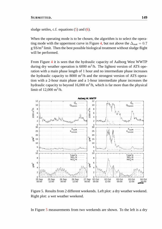
SUBMITTED . 149
sludge settles, c.f. equations (5) and (6).
When the operating mode is to be chosen, the algorithm is to select the opera-ting mode with the uppermost curve in Figure4, but not above the∆ssat= 0.7g SS/m3 limit. Then the best possible biological treatment without sludge flightwill be performed.
From Figure4 it is seen that the hydraulic capacity of Aalborg West WWTPduring dry weather operation is 6000 m3/h. The lightest version of ATS ope-ration with a main phase length of 1 hour and no intermediate phase increasesthe hydraulic capacity to 8000 m3/h and the strongest version of ATS opera-tion with a 2-hour main phase and a 1-hour intermediate phase increases thehydraulic capacity to beyond 16,000 m3/h, which is far more than the physicallimit of 12,000 m3/h.
0
2
4
6
8
10
12
1000
m3 /h
Aalborg W. WWTP
graf19.dat
QinQbypass
0
5
10
15
20
25
30
g/m
� 3
Aalborg W. WWTP
graf19.dat
XssefflXssoutat
0
2
4
6
8
10
25 Sep00:00
25 Sep12:00
26 Sep00:00
26 Sep12:00
27 Sep00:00
g/m
� 3
Aalborg W. WWTP
graf19.dat
Total NNH4-NNO3-N
0
2
4
6
8
10
12
1000
m3 /h
Aalborg W. WWTP
graf19.dat
QinQbypass
0
5
10
15
20
25
30
g/m
� 3
Aalborg W. WWTP
graf19.dat
XssefflXssoutat
0
2
4
6
8
10
02 Oct00:00
02 Oct12:00
03 Oct00:00
03 Oct12:00
04 Oct00:00
g/m
� 3
Aalborg W. WWTP
graf19.dat
Total NNH4-NNO3-N
Figure 5. Results from 2 different weekends. Left plot: a dry weather weekend.Right plot: a wet weather weekend.
In Figure5 measurements from two weekends are shown. To the left is a dry

150 PAPER F
weather weekend with dry weather operation of the plant and to the right a wetweather example with ATS operation during some of the period (from Octo-ber 2nd 10:14 to October 3rd 14:08, and October 3rd 11:44 to 14:08). Thealgorithm controlling the phase lengths of ATS operation is an earlier devel-oped version than the one proposed here. The uppermost graphs show theinfluent flow to the aeration tanks as well asQbypass, which is the part of thetotal inflow to the WWTP that bypasses the biological treatment. In the middlegraphs, the SS concentration in the effluent from the aeration tanks and in theeffluent from the WWTP are shown. In the bottom graphs the ammonia andnitrate concentrations in aeration tank 6, as well as the total nitrogen concen-tration (the sum of the ammonia and nitrate concentrations) in this tank areshown. The wet weather example shows that the WWTP is actually capable ofhandling a flow of approximately 11000 m3/h. Part of the total inflow to theWWTP bypassed the biological tanks so that the plant was not flooded. Fur-thermore, it can be seen that the storm situation with ATS operation causes theammonia, nitrate and hence total nitrogen concentrations to increase to levelsconsiderable higher than during dry weather. However, the nitrogen concen-trations are below the Danish criteria for the plant (8 g total nitrogen per m3 onan average).
Economic advantages of ATS operation
Assuming that the combined system of sewers and a WWTP should be ableto handle the increase in the influent flow from 6000 m3/h to 12,000 m3/h for,say, 5 hours. Then the detention basin volume required is
5 h · 6000 m3/h = 30, 000 m3 (21)
The cost of building detention basins is estimated to be between 100 and 500Euro per m3, hence, a 30,000 m3 detention basin costs between 3,000,000 and15,000,000 Euro!

SUBMITTED . 151
Conclusions
ATS operation can be used to increase the hydraulic capacity of the WWTP andhereby decrease the need for bypassing the biological treatment facilities ofthe WWTP or adding detention basins. Compared to constructing (additional)detention basins the cost benefit of introducing ATS operation is extremelygood. Furthermore, ATS operation does not require extra space (which is notnecessarily available), does not require cleaning facilities, and does not smellbad when not in operation.
Furthermore this paper has shown how dynamic models of ATS and dry wea-ther operation can be used offline to establish and update a lookup table toselect the optimal operation strategy at the actual operating conditions in a realtime control system.
The model types used here can be applied to other types of plants and operationmodes, cf.Boonen et al.(1999); Carrette et al.(1999); Nielsen et al.(1999),and hence to develop optimal control algorithms for different plants.
Incorporation of flow and pollution flux predictions of the influent to the WWTPenables further on-line optimization of the operation, as it is then not necessaryto control the ATS phase lengths according to steady state conditions, but onlyaccording to the predicted conditions.
To predict the limiting value of the loss in the SS concentrations in the aera-tion tanks and thus the corresponding increase in the SS concentrations in thesecondary clarifier experience with the WWTP considered is required. Theinclusion of a model of the clarifier to enable better prediction of the SS con-centrations in the clarifier and when sludge flight will take place can furtherincrease the benefits of ATS operation, as it is expected that a clarifier mo-del will make it possible to operate the WWTP even closer to the point wheresludge flight occurs.

152 PAPER F
Acknowledgements
The authors wish to thank the staff of Aalborg West WWTP and the munici-pality of Aalborg for their cooperation and permission to use the data from theWWTP. Thanks are also due to Krüger A/S and the Danish Academy of Tech-nical Sciences for funding the project in connection with which the presentwork has been carried out, under grant EF-623.

Bibliography
Ashley, R. M. and Crabtree, R. W. (1992). Sediment origins, deposition andbuild-up in combined sewer systems.Water Science and Technology, 25(8),1–12. 1.1.2
Bechmann, H., Madsen, H., Poulsen, N. K., and Nielsen, M. K. (2000). Greybox modelling of first flush and incoming wastewater at a wastewater treat-ment plant.Environmetrics, 11(1), 1–12.
Bechmann, H., Nielsen, M. K., Madsen, H., and Poulsen, N. K. (1998). Con-trol of sewer systems and wastewater treatment plants using pollutant con-centration profiles.Water Science and Technology, 37(12), 87–93.
Bechmann, H., Nielsen, M. K., Madsen, H., and Poulsen, N. K. (1999a). Grey-box modelling of pollutant loads from a sewer system.UrbanWater, 1(1),71–78.
Bechmann, H., Nielsen, M. K., Poulsen, N. K., and Madsen, H. (1999b). Ef-fects and control of aeration tank settling operation. Submitted.
Bechmann, H., Nielsen, M. K., Poulsen, N. K., and Madsen, H. (1999c). Grey-box modelling of aeration tank settling. Submitted.2, 2
Berthouex, P. M. and Box, G. E. (1996). Time series models for forecast-ing wastewater treatment plant performance.Water Research, 30(8), 1865–1875. 1.1.4
Bertrand-Krajewski, J.-L., Chebbo, G., and Saget, A. (1998). Distributionof pollutant mass vs volume in stormwater discharges and the first flushphenomenon.Water Research, 32(8), 2341–2356.1.1.2
153

154 BIBLIOGRAPHY
Billmeier, E. (1986). Einfluss der Rücklaufführung auf das Absetzverhaltenbelebter Schlämme.GWF-Wasser/Abwasser, 127(5). D
Boonen, I., Bruynooghe, H., Carrette, R., Bixio, D., and Ockier, P. (1999).Renovation of the WWTP Bruges. In8th IAWQ Conference on Design, Ope-ration and Economics of Large Wastewater Treatment plants, pp. 207–214.International Association on Water Quality, IAWQ, Budapest University ofTechnology, Department of Sanitary and Environmental Engineering.2, 2
Box, G. E. P., Jenkins, G. M., and Reinsel, G. C. (1994).Time Series Analysis:Forecasting and Control. Prentice-Hall, Inc.1
Box, G. E. P. and Jenkins, J. M. (1976).Time Series Analysis: Forecasting andControl. Holden–Day, San Francisco.1, E
Bundgaard, E., Nielsen, M. K., and Henze, M. (1996). Process development byfull-scale on-line tests and documentation.Water Science and Technology,33(1), 281–287.D, 2
Capodaglio, A. G. (1994). Transfer function modelling of urban drainage sys-tems, and potential uses in real-time control applications.Water Science andTechnology, 29(1–2), 409–417.1.1.1, C
Capodaglio, A. G., Novotny, V., and Fortina, L. (1992). Modelling wastewatertreatment plants through time series analysis.Environmetrics, 3(1), 99–120.1.1.4
Carrette, R., Bixio, D., Thoeye, C., and Ockier, P. (1999). Storm operationstrategy: high-flow activated sludge process operation. In8th IAWQ Confer-ence on Design, Operation and Economics of Large Wastewater Treatmentplants, pp. 215–222. International Association on Water Quality, IAWQ, Bu-dapest University of Technology, Department of Sanitary and EnvironmentalEngineering.F, 2
Carstensen, J. and Harremoës, P. (1997). Time series modelling of overflowstructures.Water Science and Technology, 36(8–9), 45–50.1.1.3
Carstensen, J., Nielsen, M., and Strandbæk, H. (1998). Prediction of hydraulicload for urban storm control of a municipal WWT plant.Water Science andTechnology, 37(12), 363–370.A
Carstensen, J., Nielsen, M. K., and Harremoës, P. (1996). Predictive controlof sewer systems by means of grey-box models.Water Science and Techno-logy, 34(3–4), 189–194.1.1.3, A, B

BIBLIOGRAPHY 155
Chow, V. T., Maidment, D. R., and Mays, L. W. (1988).Applied Hydrology.McGraw-Hill. 1, 2.8
Conradsen, K. (1984a).An Introduction to Statistics, volume 2. Departmentof Mathematical Modelling, Technical University of Denmark, 4th edition.(In Danish: En Introduktion til Statistik).2.4
Conradsen, K. (1984b).An Introduction to Statistics, volume 1. Departmentof Mathematical Modelling, Technical University of Denmark, 5th edition.(In Danish: En Introduktion til Statistik).2.7.1
Crabtree, R. W., Ashley, R., and Gent, R. (1995). Mousetrap: Modelling ofreal sewer sediment characteristics and attached pollutants.Water Scienceand Technology, 31(7), 43–50. 1, 1.1.1, 2.8
Deletic, A. (1998). The first flush load of urban surface runoff.Water Research,32(8), 2462–2470.1.1.2
Delleur, J. W. and Gyasi-Agyei, Y. (1994). Prediction of suspended solids inurban sewers by transfer function model.Water Science and Technology,29(1–2), 171–179.1.1.1, C
Dempsey, P., Eadon, A., and Morris, G. (1997). SIMPOL: A simplified urbanpollution modelling tool. Water Science and Technology, 36(8–9), 83–88.C
Dobbs, R. A., Wise, R. H., and Dean, R. B. (1972). The use of ultra-violetabsorbance for monitoring the total organic content of water and wastewater.Water Research, 6, 1173–1180.C, C
Dupont, R. and Dahl, C. (1995). A one-dimensional model for a secondarysettling tank including density current and short-circuiting.Water Scienceand Technology, 31(2), 215–224.1.1.4, E
Dupont, R. and Sinkjær, O. (1994). Optimisation of wastewater treatmentplants by means of computer models.Water Science and Technology, 30(4),181–190. 1.1.4
EFOR Version 3.0 (1998).User’s Guide. EFOR ApS, c/o Krüger A/S, Glad-saxevej 363, DK-2860 Søborg, Denmark.1.1.4
Ekama, G. A., Barnard, J. L., Günthert, F. W., Krebs, P., McCorquodale, J. A.,Parker, D. S., and Wahlberg, E. J. (1997).Secondary settling tanks: Theory,

156 BIBLIOGRAPHY
modelling, design and operation. IAWQ Scientific and Technical ReportNo. 6. IAWQ, London. 1.1.4, E
Entem, S., Lahoud, A., Yde, L., and Bendsen, B. (1998). Real time control ofthe sewer system of Boulogne Billancourt – a contribution to improving thewater quality of the Seine.Water Science and Technology, 37(1), 327–332.1.1.1, 1.1.3
Geiger, W. F. (1987). Flushing effects in combined sewer systems. InProc.Fourth Int. Conf. Urban Storm Drainage, pp. 40–46, Lausanne.1.1.2
Gelb, A. (1974).Applied optimal estimation. MIT Press, New York.B, C, E
Grijspeerdt, K., Vanrolleghem, P., and Verstraete, W. (1995). Selection ofone-dimensional sedimentation: Models for on-line use.Water Science andTechnology, 31(2), 193–204.1.1.4, E
Grum, M. (1998). Incorporating concepts from physical theory into stochasticmodelling of urban runoff pollution.Water Science and Technology, 37(1),179–185. 1.1.1
Gujer, W., Henze, M., Mino, T., and van Loosdrecht, M. (1999). Activatedslugde model no. 3.Water Science and Technology, 39(1), 183–193. 1,1.1.4, 2.8
Gupta, K. and Saul, A. J. (1996). Specific relationships for the first flush loadin combined sewer systems.Water Research, 30(5), 1244–1252. 1.1.2,1.1.2
Härtel, L. and Pöpel, H. J. (1992). A dynamic secondary clarifier model includ-ing processes of sludge thickening.Water Science and Technology, 25(6),267–284. 1.1.4, D, E
Heip, L., Assel, J. V., and Swartenbroekx, P. (1997). Sewer flow quality mod-elling. Water Science and Technology, 36(5), 177–184.1.1.1, C
Henze, M., Grady, C. P. L., Gujer, W., v. R. Marais, G., and Matsuo, T. (1987).Activated Sludge Model No. 1. IAWPRC Scientific and Technical ReportNo. 1. IAWPRC, London.1, 1.1.4, 2.8
Henze, M., Gujer, W., Mino, T., Matsuo, T., Wentzel, M. C., and v. R. Marais,G. (1995). Activated Sludge Model No. 2. IAWQ Scientific and TechnicalReport No. 3. IAWQ, London.1, 1.1.4, 2.8
BIBLIOGRAPHY 157
Henze, M., Gujer, W., Mino, T., Matsuo, T., Wentzel, M. C., v. R. Marais,G., and van Loosdrecht, M. C. M. (1999). Activated sludge model no.2D,ASM2D. Water Science and Technology, 39(1), 165–182.1, 1.1.4, 2.8
Hernebring, C., Ohlsson, L., Andreasson, M., and Gustafsson, L.-G. (1998).Interaction between the treatment plant and the sewer system in Halmstad:Integrated upgrading based on real time control.Water Science and Techno-logy, 37(9), 127–134.1.1.1, 1.1.3
Jazwinski, A. H. (1970).Stochastic processes and filtering theory. AcademicPress.2.1, 2.5
Kanaya, T., Fujita, I., Hayashi, H., Hiraoka, M., and Tsumura, K. (1985). Au-tomatic measurement and analysis of process data in a combined wastewatertreatment plant. In Drake, R., editor,Instrumentation and control of waterand wastewater treatment and transport systems, Advances in Water Pollu-tion Control, pp. 77–84. IAWPRC, Pergamon Press.A, A, B, B, C, C
Kendall, M. G. and Stuart, A. (1979).The Advanced Theory of Statistics,volume 2. Griffin, London, 4th edition.E
Kloeden, P. and Platen, E. (1995).Numerical Solutions of Stochastic Differen-tial Equations. Springer, 2nd edition.2.2, B, C, E
Koehne, M., Hoen, K., and Schuhen, M. (1995). Modelling and simulation offinal clarifiers in wastewater treatment plants.Mathematics and Computersin Simulation, 39, 609–616. 1.1.4
Lindberg, S., Nielsen, J. B., and Carr, R. (1989). An integrated PC-modellingsystem for hydraulic analysis of drainage systems. InThe first AustralianConference on technical computing in the Water Industry: WATERCOMP’89, Melbourne, Australia.1, 1.1.1, 2.8
Liong, S. Y. and Chan, W. T. (1993). Runoff volume estimates with neuralnetworks. In Topping, B. H. V., editor,Neural Networks and CombinatorialOptimization in Civil and Structural Engineering, pp. 67–70. Civil-CompPress.1.1.1
Ljung, L. (1995). System Identification Toolbox User’s Guide. The Math-Works, Inc. Third Printing.1, 3.1
Ljung, L. (1999). System Identification, Theory for the User. Prentice Hall,New Jersey, 2nd edition.1, 2.4
158 BIBLIOGRAPHY
Madsen, H. (1995).Time Series Analysis. Department of Mathematical Mod-elling, Technical University of Denmark. (In Danish: Tidsrækkeanalyse).1, 2.7.3
Madsen, H. and Holst, J. (1996).Modelling Non-Linear and Non-StationaryTime Series. Department of Mathematical Modelling, Department of Mathe-matical Modelling. 2.1, 2.2, 2.2
Madsen, H. and Melgaard, H. (1991). The mathematical and numerical me-thods used in CTLSM – a program for ML-estimation in stochastic, con-tinuous time dynamical models. Technical Report no. 7/1991, Institute ofMathematical Statistics and Operations Research, Technical University ofDenmark, Lyngby, Denmark.3.1, B, B, B, C, C, E, E
Madsen, H., Nielsen, J. N., and Baadsgaard, M. (1998).Statistics in Finance.Department of Mathematical Modelling, Technical University of Denmark.2.2, 2.5, 2.5
Mark, O., Appelgren, C., and Larsen, T. (1995). Principles and approachesfor numerical modelling of sediment transport in sewers.Water Science andTechnology, 31(7), 107–115.1, 1.1.1, 2.8, C
Mark, O., Hernebring, C., and Magnusson, P. (1998a). Optimisation and con-trol of the inflow to a wastewater treatment plant using integrated modellingtools. Water Science and Technology, 37(1), 347–354.1.1.1
Mark, O., Wennberg, C., van Kalken, T., Rabbi, F., and Albinsson, B. (1998b).Risk analyses for sewer systems based on numerical modelling and GIS.Safety Science, 30(1998), 99–106.1, 1.1.1, 1.1.3, 2.8
Matsché, N. and Stumwöhrer, K. (1996). UV absorption as control-parameterfor biological treatment plants.Water Science and Technology, 33(12), 211–218. A, A, B, B, C, C
Meinholz, T. L., Hansen, C. A., and Novotny, V. (1974). An application of thestorm water management model. In Kao, D. T. Y., editor,Proceedings of theNational Symposion on Urban Rainfall and Runoff and Sediment Control,pp. 109–113. University of Kentucky.1.1.1
Melgaard, H. (1994).Identification of Physical Models. Ph.D. thesis, Instituteof Mathematical Modelling, Technical University of Denmark. No. 1994–4.2.1, 2.7.3

BIBLIOGRAPHY 159
Melgaard, H. and Madsen, H. (1991). CTLSM version 2.6 – a program forparameter estimation in stochastic differential equations. Technical Reportno. 1/1993, Institute of Mathematical Statistics and Operations Research,Technical University of Denmark, Lyngby, Denmark.3.1, B
Melgaard, H. and Madsen, H. (1993). CTLSM continuous time linear stocha-stic modelling. In Bloem, J., editor,In: Workshop on Application of SystemIdentification in Energy Savings in Buildings, pp. 41–60. Institute for Sys-tems Engineering and Informatics, Joint Research Centre, Ispra, Italy.B,C, E
Mrkva, M. (1975). Automatic U.V.-control system for relative evaluation oforganic water pollution.Water Research, 9, 587–589. C, C
Nielsen, M. and Önnerth, T. (1995). Improvement of a recirculating plant byintroducing STAR control.Water Science and Technology, 31(2), 171–180.1.1.5, C, D, E, E
Nielsen, M. K., Bechmann, H., and Henze, M. (1999). Modelling and testof Aeration Tank Settling ATS. In8th IAWQ Conference on Design, Ope-ration and Economics of Large Wastewater Treatment plants, pp. 199–206.International Association on Water Quality, IAWQ, Budapest University ofTechnology, Department of Sanitary and Environmental Engineering.E, 2,2, 2
Nielsen, M. K., Carstensen, J., and Harremoës, P. (1996). Combined control ofsewer and treatment plant during rainstorm.Water Science and Technology,34(3), 181–187.D, 5, 2
Nouh, M. (1996). Simulation of water quality in sewer flows by neural net-works. In Müller, editor,Proceedings of the second int. conf. Hydroinfor-matics. Hydroinformatics ’96, volume 2, pp. 885–891, Balkema, Rotterdam.1.1.1
Novotny, V., Jones, H., Feng, X., and Capodaglio, A. (1991). Time seriesanalysis models of activated sludge plants.Water Science and Technology,23, 1107–1116.1.1.4
Nowack, G. and Ueberbach, O. (1995). Die kontinuierliche SAK-MessungAussagekraft, Statistik und Anwendungen.Korresspondenz Abwasser,42(11), 2020–2030.A, A, B, B, C, C

160 BIBLIOGRAPHY
Øksendal, B. (1995).Stochastic Differential Equations. Springer, 4th edition.2.1, 2.2, B, C, E
Olsson, G. (1992). Control of wastewater treatment systems.ISA Transactions,31(1), 87–96. 1.1.5
Olsson, G., Andersson, B., Hellström, B. G., Holmström, H., Reinius, L. G.,and Vopatek, P. (1989). Measurements, data analysis and control methodsin wastewater treatment plants – state of the art and future trends.WaterScience and Technology, 21, 1333–1345.1.1.5
Önnerth, T. and Bechmann, H. (1995). Implementation of and results fromadvanced on-line computer control of a BNR recirculating plant. InNewand emerging environmental technologies and products conference for was-tewater treatment and stormwater collection, volume 11, pp. 51–72. WaterEnvironment Federation.1.1.5, C, E, E
Poulsen, N. K. (1995).Stochastic Adaptive Control. Department of Mathema-tical Modelling, Technical University of Denmark. (In Danish: Stokastiskadaptiv regulering).1
Pu, H.-C. and Hung, Y.-T. (1995). Use of artificial neural networks: predic-ting trickling filter performance in a municipal wastewater treatment plant.Environmental Management and Health, 6(2), 16–27. 1.1.4
Rangla, M. K., Burnham, K. J., and Stephens, R. I. (1998). Simulation ofactivated sludge process control strategies. InInternational Conference onSimulation ’98, pp. 152–157. IEE. IEE Conf. Publ. No. 457.1.1.4
Reynolds, D. M. and Ahmad, S. R. (1997). Rapid and direct determinationof wastewater BOD values using a fluorescence technique.Water Research,31(8), 2012–2018.C, C
Ruan, M. and Wiggers, J. B. M. (1997). Application of time-series analysisto urban storm drainage.Water Science and Technology, 36(5), 125–131.1.1.1, C
Ruban, G., Marchandise, P., and Scrivener, O. (1993). Pollution measurementaccuracy using real time sensors and wastewater samples analysis.WaterScience and Technology, 28(11–12), 67–78.A, A, B, B, C, C
Saget, A., Chebbo, G., and Bertrand-Krajewski, J.-L. (1996). The first flush insewer systems.Water Science and Technology, 33(9), 101–108.1.1.2
BIBLIOGRAPHY 161
Sjöberg, J., Zhang, Q., Ljung, L., Benveniste, A., Delyon, B., Glorennec, P.-Y.,Hjalmarsson, H., and Juditsky, A. (1995). Nonlinear black-box modeling insystem identification: a unified overview.Automatica, 31(12), 1691–1724.1
Takács, L., Patry, G. G., and Nolasco, D. (1991). A dynamic model of thethickening/clarification process.Water Research, 25, 1263–1271.1.1.4
van Luijtelaar, H. and Rebergen, E. W. (1997). Guidelines for hydrodynamiccalculations on urban drainage in The Netherlands: Backgrounds and exam-ples.Water Science and Technology, 36(8–9), 253–258.C
Vesilind, P. A. (1968). Design of prototype thickeners from batch settling tests.Water & Sewage Works, 115, 302–307. 1.1.4, E, E, 2
Vesilind, P. A. (1979). Treatment and disposal of wastewater sludge. AnnArbor Science, 1st edition.1.1.4, D, E
Ward, W., Vaccari, D. A., McMahon, D., Rivera, S., and Wojciechowski, E.(1996). A hybrid deterministic/nonlinear stochastic model of the activatedsludge proces. In Zannetti, P. and Brebbia, C. A., editors,Developmentand Application of Computer Techniques to Environmental Studies VI, pp.81–90. IEE, Comput. Mech. Publications.1.1.4
Wass, P. D., Marks, S. D., Finch, J. W., Leeks, G. J. L., and Ingram, J. K.(1997). Monitoring and preliminary interpretation of in-river turbidity andremote sensed imagery for suspended sediment transport studies in the Hum-ber catchment.The Science of the Total Environment, 194–195, 263–283.C, C
Wett, B., Gluderer, D., and Rauch, W. (1997). Denitrifikation beim Absetzvor-gang.GWF-Wasser/Abwasser, 138(7). D
Young, P. and Wallis, S. (1985). Recursive estimation: A unified approachto the identification, estimation, and forecasting of hydrological systems.Applied Mathematics and Computation, 17, 299–334. 1
Young, P. C., Jakeman, A. J., and Post, D. A. (1997). Recent advances in thedata-based modelling and analysis of hydrological systems.Water Scienceand Technology, 36(5), 99–116. 1, C
Zhao, H., Hao, O. J., and McAvoy, T. J. (1999). Approaches to modellingnutrient dynamics: ASM2, simplified model and neural nets.Water Scienceand Technology, 39(1), 227–234.1.1.4

162 BIBLIOGRAPHY
Ph.D. theses from IMM
1. Larsen, Rasmus. (1994). Estimation of visual motion in image se-quences. xiv+ 143 pp.
2. Rygard, Jens Moberg. (1994). Design and optimization of flexiblemanufacturing systems. xiii+ 232 pp.
3. Lassen, Niels Christian Krieger. (1994). Automated determination ofcrystal orientations from electron backscattering patterns. xv+ 136 pp.
4. Melgaard, Henrik. (1994). Identification of physical models. xvii+246 pp.
5. Wang, Chunyan. (1994). Stochastic differential equations and a bio-logical system. xxii+ 153 pp.
6. Nielsen, Allan Aasbjerg. (1994).Analysis of regularly and irregularlysampled spatial, multivariate, and multi-temporal data. xxiv+ 213 pp.
7. Ersbøll, Annette Kjær. (1994). On the spatial and temporal correla-tions in experimentation with agricultural applications. xviii+ 345 pp.
8. Møller, Dorte. (1994). Methods for analysis and design of heteroge-neous telecommunication networks.Volume 1-2,xxxviii + 282 pp., 283-569 pp.
9. Jensen, Jens Christian. (1995). Teoretiske og eksperimentelle dy-namiske undersøgelser af jernbanekøretøjer. viii+ 174 pp.
10. Kuhlmann, Lionel. (1995).On automatic visual inspection of reflectivesurfaces.Volume 1,xviii + 220 pp., (Volume 2,vi + 54 pp., fortrolig).
163

164 PH .D. THESES FROM IMM
11. Lazarides, Nikolaos. (1995). Nonlinearity in superconductivity andJosephson Junctions. iv+ 154 pp.
12. Rostgaard, Morten. (1995). Modelling, estimation and control of fastsampled dynamical systems. xiv+ 348 pp.
13. Schultz, Nette. (1995). Segmentation and classification of biologicalobjects. xiv+ 194 pp.
14. Jørgensen, Michael Finn.(1995).Nonlinear Hamiltonian systems. xiv+ 120 pp.
15. Balle, Susanne M.(1995). Distributed-memory matrix computations.iii + 101 pp.
16. Kohl, Niklas. (1995). Exact methods for time constrained routing andrelated scheduling problems. xviii+ 234 pp.
17. Rogon, Thomas.(1995). Porous media: Analysis, reconstruction andpercolation. xiv+ 165 pp.
18. Andersen, Allan Theodor. (1995). Modelling of packet traffic withmatrix analytic methods. xvi+ 242 pp.
19. Hesthaven, Jan.(1995).Numerical studies of unsteady coherent struc-tures and transport in two-dimensional flows.Risø-R-835(EN) 203 pp.
20. Slivsgaard, Eva Charlotte. (l995). On the interaction between wheelsand rails in railway dynamics. viii+ 196 pp.
21. Hartelius, Karsten. (1996). Analysis of irregularly distributed points.xvi + 260 pp.
22. Hansen, Anca Daniela.(1996). Predictive control and identification -Applications to steering dynamics. xviii+ 307 pp.
23. Sadegh, Payman.(1996).Experiment design and optimization in com-plex systems. xiv+ 162 pp.
24. Skands, Ulrik. (1996). Quantitative methods for the analysis of elec-tron microscope images. xvi+ 198 pp.
25. Bro-Nielsen, Morten. (1996). Medical image registration and surgerysimulation. xxvii+ 274 pp.

PH .D. THESES FROM IMM 165
26. Bendtsen, Claus.(1996).Parallel numerical algorithms for the solutionof systems of ordinary differential equations. viii+ 79 pp.
27. Lauritsen, Morten Bach. (1997).Delta-domain predictive control andidentification for control. xxii+ 292 pp.
28. Bischoff, Svend.(1997).Modelling colliding-pulse mode-locked semi-conductor lasers. xxii+ 217 pp.
29. Arnbjerg-Nielsen, Karsten. (1997). Statistical analysis of urban hy-drology with special emphasis on rainfall modelling.Institut for Miljø-teknik, DTU.xiv + 161 pp.
30. Jacobsen, Judith L.(1997). Dynamic modelling of processes in riversaffected by precipitation runoff. xix+ 213 pp.
31. Sommer, Helle Mølgaard.(1997).Variability in microbiological degra-dation experiments - Analysis and case study. xiv+ 211 pp.
32. Ma, Xin. (1997).Adaptive extremum control and wind turbine control.xix + 293 pp.
33. Rasmussen, Kim Ørskov.(1997). Nonlinear and stochastic dynamicsof coherent structures. x+ 215 pp.
34. Hansen, Lars Henrik. (1997).Stochastic modelling of central heatingsystems. xxii+ 301 pp.
35. Jørgensen, Claus. (1997). Driftsoptimering på kraftvarmesystemer.290 pp.
36. Stauning, Ole. (1997). Automatic validation of numerical solutions.viii + 116 pp.
37. Pedersen, Morten With. (1997).Optimization of recurrent neural net-works for time series modeling. x+ 322 pp.
38. Thorsen, Rune. (1997). Restoration of hand function in tetraplegicsusing myoelectrically controlled functional electrical stimulation of thecontrolling muscle. x+ 154 pp. + Appendix.
39. Rosholm, Anders. (1997). Statistical methods for segmentation andclassification of images. xvi+ 183 pp.
166 PH .D. THESES FROM IMM
40. Petersen, Kim Tilgaard. (1997). Estimation of speech quality in tele-communication systems. x+ 259 pp.
41. Jensen, Carsten Nordstrøm.(1997). Nonlinear systems with discreteand continuous elements.195 pp.
42. Hansen, Peter S.K.(1997). Signal subspace methods for speech en-hancement. x+ 226 pp.
43. Nielsen, Ole Møller. (1998). Wavelets in scientific computing. xiv+232 pp.
44. Kjems, Ulrik. (1998).Bayesian signal processing and interpretation ofbrain scans. iv+ 129 pp.
45. Hansen, Michael Pilegaard. (1998). Metaheuristics for multiple ob-jective combinatorial optimization. x+ 163 pp.
46. Riis, Søren Kamaric. (1998). Hidden markov models and neural net-works for speech recognition. x+ 223 pp.
47. Mørch, Niels Jacob Sand. (1998). A multivariate approach to func-tional neuro modeling. xvi+ 147 pp.
48. Frydendal, Ib. (1998.) Quality inspection of sugar beets using vision.iv + 97 pp. + app.
49. Lundin, Lars Kristian. (1998).Parallel computation of rotating flows.viii + 106 pp.
50. Borges, Pedro. (1998). Multicriteria planning and optimization. -Heuristic approaches. xiv+ 219 pp.
51. Nielsen, Jakob Birkedal. (1998). New developments in the theory ofwheel/rail contact mechanics. xviii+ 223 pp.
52. Fog, Torben. (1998).Condition monitoring and fault diagnosis in ma-rine diesel engines. xii+ 178 pp.
53. Knudsen, Ole.(1998).Industrial vision. xii+ 129 pp.
54. Andersen, Jens Strodl. (1998). Statistical analysis of biotests. - Ap-plied to complex polluted samples. xx+ 207 pp.
PH .D. THESES FROM IMM 167
55. Philipsen, Peter Alshede. (1998). Reconstruction and restoration ofPET images. vi+ 132 pp.
56. Thygesen, Uffe Høgsbro.(1998).Robust performance and dissipationof stochastic control systems.185 pp.
57. Hintz-Madsen, Mads. (1998). A probabilistic framework for classifi-cation of dermatoscopic images. xi+ 153 pp.
58. Schramm-Nielsen, Karina.(1998).Environmental reference materialsmethods and case studies. xxvi+ 261 pp.
59. Skyggebjerg, Ole. (1999). Acquisition and analysis of complex dyna-mic intra- and intercellular signaling events.83 pp.
60. Jensen, Kåre Jean.(1999).Signal processing for distribution networkmonitoring. x+ 140 pp.
61. Folm-Hansen, Jørgen.(1999).On chromatic and geometrical calibra-tion. xiv+ 241 pp.
62. Larsen, Jesper. (1999). Parallelization of the vehicle routing problemwith time windows.xx+ 266 pp.
63. Clausen, Carl Balslev.(1999).Spatial solitons in quasi-phase matchedstruktures. vi+ (flere pag.)
64. Kvist, Trine. (1999).Statistical modelling of fish stocks. xiv+ 173 pp.
65. Andresen, Per Rønsholt. (1999). Surface-bounded growth modelingapplied to human mandibles. xxii+ 116 pp.
66. Sørensen, Per Settergren.(1999).Spatial distribution maps for benthiccommunities.
67. Andersen, Helle.(1999).Statistical models for standardized preclinicalstudies. viii+ (flere pag.)
68. Andersen, Lars Nonboe. (1999). Signal processing in the dolphinsonar system. xii+ 214 pp.
69. Bechmann, Henrik. (1999). Modelling of wastewater systems. xviii+161 pp.

168 PH .D. THESES FROM IMM