CDE August, 2007

Modelling Seasonal Dynamics in Indian Industrial Production: An Extention of TV-STAR Model

Pami Dua Email: dua@econdse.org

Department of Economics, Delhi School of Economics

&

Lokendra Kumawat Email: lokendrak@gmail.com

Department of Economics, Ramjas College,

University of Delhi, Delhi-110 007

Working Paper No. 162

Centre for Development Economics

Department of Economics, Delhi School of Economics

Modelling Seasonal Dynamics in Indian Industrial Production:

An Extention of TV-STAR Model

Pami Dua∗

Professor, Department of Economics, Delhi School of Economics,

University of Delhi, Delhi 110 007

Lokendra Kumawat

Lecturer, Department of Economics, Ramjas College,

University of Delhi, Delhi - 110 007

Abstract

This paper models the seasonal dynamics in quarterly industrial production

for India. For this, we extend the time-varying smooth transition autoregression

(TV-STAR) model to allow for independent regime-switching behaviour in the

deterministic seasonal and cyclical components. This yields the time-varying

seasonal smooth transition (TV-SEASTAR) model. We find evidence of the

effect of rainfall growth on seasonal dynamics of industrial production. We

also find that the seasonal dynamics have changed over the past decade, one

aspect of this being the significant narrowing down of seasonals. The timing of

these changes coincides with the changes in the character of the economy as it

progressed towards a free-market economy in the post liberalization period.

JEL Classification Code: C22

Keywords: Seasonality, Smooth transition autoregression, Economic

reforms.

∗The authors are grateful to Sunil Kanwar and Abhijit Banerji for useful discussions.

1

1 Introduction

Seasonality is an important component of industrial output in many countries, and at

times swamps other movements. However, until recently, seasonality was considered to be

very regular and therefore devoid of any economic information. This led to the practice

of seasonal adjustment before the series was used for further analysis. Since it has now

been recognized that seasonal fluctuations are not very regular and may contain important

information about the economy, attempts have been made to model seasonality in output.

Seasonality has special relevance to the Indian economy due to the predominant role of

agriculture in the economy. Though agriculture contributes only 24% to total output, it

accounts for 60% of the total labour force that depend on agriculture for their livelihood.

Due to the lack of irrigation facilities, the agriculture depends heavily on rainfall, the

bulk of which comes in two seasons: June-September and December-February. This

dependence on rainfall imparts to agriculture a high degree of seasonality. Thus, any

activity which has strong linkages with agriculture, including industrial production, is

also expected to be seasonal.

Attempts to study the dynamics of Indian industrial production at the sub-annual

frequency have shown that it has a high degree of seasonality, but that seasonality varies

over time. While Sinha and Kumawat (2004) have shown that seasonality in output is

stochastic, Dua and Kumawat (2005) show that besides being stochastic, it is also related

to the stochastic trend. The latter study also finds that industrial production is much

more volatile in the first two quarters of the calender year, which correspond to highest

and lowest industrial production respectively, as compared to the last two. The authors

suggest that this is due to the fact that industrial production is related to agricultural

production. This in turn, depends heavily on rainfall, which is highly volatile. Therefore,

agricultural production is also very volatile and this causes high volatiilty in industrial

output as well.

van Dijk et. al (2001, VST henceforth) identify two types of changes in seasonals:

cyclical changes caused by the stage of the business cycle, and secular changes caused

by gradual institutional and technological changes. For the Indian economy, the cyclical

changes are influenced both by the stage of the business cycle as well as the performance

of agriculture, which, in turn, depends on rainfall. Similarly, the secular change caused

by technological and institutional changes also appear to be important, particularly in

view of the substantial marked-oriented reforms introduced in the early 1990s. Thus, the

2

framework adopted by VST appears to be relevant here as well, after making allowance

for the variation due to rainfall.

The objective of this paper is to model the seasonal dynamics of industrial production

in the Indian economy. Specifically, we consider two types of factors. First, we test for the

effects of agricultural performance and the stage of the business cycle on the seasonals to

extend the results of Dua and Kumawat (2005) that show that the seasonality in Indian

industrial production is caused by the agricultural cycle and is affected by rainfall and

the stage of business cycle. Next, we test whether this has been changing over time,

particularly after the market-oriented reforms introduced in early 1990s. Though this

fits largely in the framework of VST, we estimate a more general model. In contrast

to VST’s model, our model allows for independent regime-switching behaviour in the

deterministic seasonal and cyclical components, and then smooth time variation in this

behaviour itself. Thus, our model nests both the seasonal STAR (SEASTAR) model of

Franses et. al (2000) and the time-varying STAR (TV-STAR) model of VST, and can

therefore be called the time-varying seasonal STAR (TV-SEASTAR) model.

We find that the seasonals in the industrial production are driven mainly by the rate

of growth of rainfall and that of an indicator of economic activity to capture the stage of

the business cycle. This is measured by the annual growth in the industrial production.

However, in the past one decade, while seasonals appear to have stabilised substantially,

their character has changed.

The paper is organised as follows: the following section contains some discussion about

the Indian economy. It starts with a discussion of the seasonal character of the Indian

economy and the literature pertaining to that. This is followed by a brief discussion of

gradual changes in the character of the economy. Section 3 discusses the basic smooth

transition autoregression and its extension proposed by us, viz., the TV-SEASTAR model.

Section 4 discusses the methodology of this paper, followed by the discussion of data.

Section 5 presents the empirical results. Section 6 concludes.

2 Salient characteristics of the Indian economy

2.1 Seasonal Character of the Indian economy and industrial production

The Indian economy is highly seasonal. This is mainly due to the predominantly agricul-

tural character of the economy. Though agriculture contributes only 24% of total output,

3

it employs more than 60% of its workforce. Due to the lack of irrigation facilities, agricul-

ture depends heavily on rainfall. Rainfall occurs mainly in two seasons: June-September

(summer season) and December-February (winter season). Therefore, agricultural activ-

ity is also concentrated in these two seasons only. The summer rainfall covers a larger

area and therefore the crop taken in this season, called the Kharif crop, has a larger share

in total agricultural output. The other crop, called the Rabi crop is more dependent on

irrigation facilities and has a lower share, though of late the gap between the two has been

declining. Due to the high volatility of the quantum as well as the distribution of rainfall,

the crops, particularly the Kharif crop also shows huge fluctuations. These fluctuations

affect the rest of the economy through both forward and backward linkages. Specifically,

agriculture provides raw materials for a large number of industries. On the other hand,

as a major part of the population is dependent on agriculture for its livelihood, this

sector is a significant source of demand for industrial products. Thus, agriculture plays

a dominant role in shaping the seasonal as well as other fluctuations in the industrial

production. Therefore industrial production is influenced heavily by the timing as well

as the variation in rainfall.

The above is clearly reflected in the highly seasonal nature of industrial production.

The first quarter is the highest industrial activity quarter, while the second quarter

corresponds to the lowest level of industrial output. The industrial activity then rises

gradually in the third and fourth quarters. In other words, the industrial production

is lowest in the second quarter and then rises gradually, attaining its peak in the first

quarter.

Further, the seasonals are not constant over time. Sinha and Kumawat (2004) found

statistical evidence for nonstationarity of seasonality. Dua and Kumawat (2005) note

two important features of these seasonal fluctuations: first, stochastic seasonality is not

independent of stochastic trend; and second, the volatility of industrial output too varies

with seasons. Specifically, the volatility is more in the first two quarters as compared to

the last two. The authors opine that the reasons for the high level as well as the high

volatility of industrial output in the first quarter is mainly due to the fact that industrial

activity in the last and the first quarter is powered by the agricultural performance in the

Kharif season. This is due to inputs for the industrial sector coming from agriculture, as

well as the demand originating for the industral sector in the agriculture sector due to

the Kharif crop. While this causes the industrial production to attain its intra-year peak

4

in the first quarter, the high volatility of rainfall and therefore the Kharif output renders

it highly volatile. The second quarter does not witness any activity in the agricultural

sector, and therefore industrial activity is also low in that season.

2.2 Gradual changes in the character of the economy

The character of the Indian economy has been changing gradually right since the time

of India’s freedom from the British rule in 1947. At that time, the Indian economy was

primarily an agricultural economy. Gradually, the share of agriculture in India’s national

output declined1, while that of industry, and even more, that of services rose2. Even the

character of agriculture has been changing gradually, and one important aspect of this is

the decline in its dependence on rainfall, due to the increasing availability of irrigation

facilities3. Thus, not only has the dependence of the economy on agriculture fallen, the

dependence of the latter on rainfall has also fallen. Both of these have reduced the

dependence of the economy on natural forces. This was supplemented (to some extent,

also facilitated) by a number of measures taken by the government towards liberalization,

privatization and globalisation of the economy, starting in 1991. These measures changed

the face of the economy completely from a state-controlled closed economy to an open,

market economy. Clearly such a transformation would be reflected in the dynamics of

the industrial output as well.

The above discussion suggests that both types of changes in the seasonality suggested

by VST appear to be important for the Indian economy. On the one hand, seasonals

appear to be affected by the growth of rainfall and that of economic activity. On the

other hand, there is a possibility of this pattern having changed in the past few years.

Therefore, the seasonals can be modeled in the framework of the time-varying smooth

transition autoregression suggested by VST.

1The share of agriculture in India’s GDP was about 50% in 1950-51. From that level, it fell to 33% in 1980-81, 27% in

1990-91 and 16% in 2006-07.2From a level of 33% in 1950-51, the share of services in India’s GDP rose to 40% in 1980-81 and 44% in 1990-91. It

rose sharply after that and stood at 55% in 2006-07, thus accounting for more than half of India’s GDP.3The share of gross irrigated area in gross cropped area rose from 23% in 1970-71 to 29% in 1980-81, 34% in 1990-91

and 41% in 2002-03.

5

3 Smooth Transition Autoregression and its extensions

3.1 Basic STAR Model

We begin with an AR model with seasonally varying intercepts,

yt = α0 +4∑

i=1

αiSit +p∑

i=1

βiyt−i + εt (1)

where Sit = Dit − D1t, Dit being a seasonal dummy that takes the value 1 in the ith

season and 0 otherwise4. To allow for smooth transition in the seasonal and cyclical

components according to a transition function F (xt, γ, µ) whose value varies smoothly

between 0 and 1 as the variable x varies in the interval (−∞,∞), we get an extension of the

smooth transition autoregression (STAR) suggested by Terasvirta and Anderson (1992).

Specifically, if we choose this function (transition function) to be a logistic function5

F (xt, γ, µ) =1

1 + exp{−γ(xt − µ)}, γ > 0, (2)

we get an extension of the the logistic STAR (LSTAR) model. Allowing for separate

transition functions, Fs(xst, γs, µs) and Fc(xct, γc, µc) for the seasonal part and cyclical

parts respectively, we obtain the SEASTAR model of Franses and van Dijk (2000):

yt =

(4∑

i=1

α0iSit

)(1− Fs(xst, γs, µs)) +

(4∑

i=1

α1iSit

)Fs(xst, γs, µs)

+

( p∑i=1

β0iyt−i

)(1− Fc(xct, γc, µc)) +

( p∑i=1

β1iyt−i

)Fc(xct, γc, µc) + εt (3)

where we have written S1t for intercept for brevity of notation. Looking at the seasonal

component, for instance, for very low values of xst, Fs(xst, γs, µs) is equal to zero, so that

the coefficient of Sit is α0i. On the other hand, for sufficiently large values of xst, the

value of Fs(xst, γs, µs) is equal to unity, so that the coefficient of Sit is equal to α1i. In

between, as the value of xst varies from very low to very high, the value of the transition

function varies from 0 to 1. The coefficient of Sit is a weighted sum of the two values α0i

and α1i, the weight depending on the value of xst and also the two parameters γs and

µs, called smoothness and location parameter, respectively. The smoothness parameter

governs the speed of transition; for very high values of γs the transition function changes

its value from 0 to 1 abruptly, as the xst crosses the value of the location parameter. On4We take these dummies instead of taking Dit since in this specification the coefficients denote deviations of seasons

from the average intercept. Thus seasonal patterns can be seen directly from the coefficient values. The corresponding

value for the first season is equal to −(α2 + α3 + α4).5The properties of this function have been documented extensively, and therefore are not being discussed here. See, for

example, Terasvirta and Anderson (1992) and Terasvirta (1994).

6

the other hand, for low values of γs, Fs(xst, γs, µs) changes values slowly from 0 to 1; the

smaller is the value of γs, the slower is the transition.

Though the above specification shows clearly the values of different coefficients in

different regimes, it does not show which coefficients undergo regime-switching; for that

we have to test the significance of the difference between α0i and α1i separately for each

coefficient. Therefore, we modify the specification slightly to get

yt =

(4∑

i=1

α0iSit

)+

(4∑

i=1

α2iSit

)Fs(xst, γs, µs)

+

( p∑i=1

β0iyt−i

)+

( p∑i=1

β2iyt−i

)Fc(xct, γc, µc) + εt (4)

where α2i = α1i − α0i and β2i = β1i − β0i. Thus if α2i is statistically significant, this

shows significant changes in the coefficient of Sit across the regimes.

3.2 Extensions of the STAR Model

To allow for gradual institutional and technological changes, the above model needs to be

extended by allowing for gradual changes in the above structure. Due to the lack of any

better indicator, VST suggest that these changes can be captured by the time variable

itself. This means that we have to estimate the following type of model:

yt =

((4∑

i=1

α00iSit

)+

(4∑

i=1

α02iSit

)Fs(xst, γs, µs)

)(1− Fst(t, γst, µst))

+

((4∑

i=1

α10iSit

)+

(4∑

i=1

α12iSit

)Fs(xst, γs, µs)

)Fst(t, γst, µst)

+

(( p∑i=1

β00iyt−i

)+

( p∑i=1

β02iyt−i

)Fc(xct, γc, µc)

)(1− Fct(t, γct, µct))

+

(( p∑i=1

β10iyt−i

)+

( p∑i=1

β12iyt−i

)Fc(xct, γc, µc)

)Fct(t, γct, µct)

+ εt (5)

Again, following the reasons behind the steps to equation (4) from equation (3), the above

can be reorganised to get

yt =

((4∑

i=1

α00iSit

)+

(4∑

i=1

α02iSit

)Fs(xst, γs, µs)

)

+

((4∑

i=1

α20iSit

)+

(4∑

i=1

α22iSit

)Fs(xst, γs, µs)

)Fst(t, γst, µst)

+

(( p∑i=1

β00iyt−i

)+

( p∑i=1

β02iyt−i

)Fc(xct, γc, µc)

)

7

+

(( p∑i=1

β20iyt−i

)+

( p∑i=1

β22iyt−i

)Fc(xct, γc, µc)

)Fct(t, γct, µct)

+ εt (6)

Thus α20i and α22i represent changes in the seasonal dynamics over time. Specifically,

while α20i represents how seasonals have changed in the period characterised by low

values of the transition variable (called the ‘base period’ for brevity), α22i shows how the

regime-switching behaviour itself has changed over time. This model is an extension

of the TV-STAR model proposed by VST in that it allows for different type of

regime-switching behaviour in the seasonal and cyclical components. In this

sense, it encompasses both the TV-STAR model suggested by VST and the

SEASTAR model suggested by Franses et. al (2000) and can be appropriately

called the time-varying seasonal STAR (TV-SEASTAR) model6.

One important point needs clarification. It might be asked why we are allowing for

regime-switching in the cyclical component when our focus is on seasonal fluctuations.

There are two reasons for this. First, seasonality is stochastic in many cases (even if

stationary) and this will be captured by the structure7. Not allowing for regime-switching

in that will cause the regime-switching to be detected spuriously in the deterministic

seasonal component. Secondly, there is empirical evidence for asymmetric behaviour of

industrial production over phases of business cycles for several countries including India

(see, for example, Sinha and Kumawat, 2005). Again, this would lead to bias in the

results of nonlinearity in the seasonal component if we do not make allowance for regime-

switching in the cyclical part.

One final observation on why we allow for different types of regime-switching in sea-

sonal and cyclical components, i.e., why we need to extend the TV-STAR model. The

reason is that the factors that explain a regime-switch in seasonals might be different

from the corresponding factors for the cyclical component. Franses and van Dijk (2000)

find empirical support for this. Using the same transition function (TF) for the two

components in such cases would lead to biased results.

6To our knowledge this model has not been used by anyone so far.7That’s why we call the AR component the ‘cyclical’ component and not ‘non-seasonal’ component.

8

4 Methodology and Data

4.1 Methodology

In this paper we model the seasonal dynamics in the index of industrial production (IIP)

for India. Due to the clear trend in this variable, which has been shown to be stochastic

(Sinha and Kumawat, 2004 and Dua and Kumawat, 2005), we consider the first difference

of log IIP. The procedure is as follows:

1. We begin with a linear AR model with seasonally varying intercepts, given in equa-

tion (1). The order of autoregression is determined on the basis of AIC, SIC and

LM test for residual serial correlation.

2. In the next step, we carry out a test for nonlinearity. This test cannot be done using

the standard Wald test, since under the null hypothesis of no nonlinearity (γs = 0),

the parameters µs and α2i are not identified 8. Therefore the test is carried out

as per the procedure suggested by Terasvirta and Anderson (1992) and Terasvirta

(1994), using the Taylor series approximation of the logistic function.

3. The SEASTAR models given in equation (4) are then estimated. Estimation is

carried out in two steps. The initial values are first refined using the simplex method.

This is followed by the application of the restricted BFGS method.

4. The models thus estimated are subjected to tests for serial correlation (first and

fourth order). Again, these tests cannot be performed in a conventional manner, but

are derived following the procedure suggested by Eitrheim and Terasvirta (1996).

5. The models thus obtained are extended to allow for time-variation, thus obtaining

the TV-SEASTAR models.

One important aspect of the methodology is the selection of transition variables (xst

and xct, for instance). The discussion in Section 2 above suggests two types of economic

indicators for regime-switching behaviour here. First, the level of industrial activity,

which is measured by the fourth difference of log IIP9 and its lags. The other indicator,

8The other way to test for no nonlinearity would be to test α2i = 0 ∀i. However, in that case γs and µs are not

identified.9It may be noted that our dependent variable is the first differenced log IIP, while as an indicator of business cycle,

we take the fourth differenced log IIP. The latter is due to the fact that for India, quarterly data for other such variables,

e.g. GDP, is not available for a long enough period. This should not affect our ersults since the objective is to model the

seasonal behaviour of IIP. The annual growth rate of IIP merely serves as a proxy for overall economic activity.

9

as suggested by the discussion in Section 2, is an indicator of rainfall. For this we use

the annual rate of growth of rainfall. In the following discussion, we denote the fourth

difference of log IIP by 44yt and the annual rate of growth of rainfall by Rt. Thus, we

have two types of transition variables: lags of 44yt and of Rt.

4.2 Data

The data for the index of industrial production is taken from the Reserve Bank of India

database. We take quarterly data for the period 1981Q1 to 2006Q4. Data on rainfall is

taken from the website www.indiastat.com and various issues of the Monthly Review of

the Centre for Monitoring Indian Economy (CMIE).

5 Empirical Results

5.1 Graphical Analysis

We first examine the plot of seasonals in Figure 1. This presents the moving four-year

average of the deviations of the seasonal means from the annual average. These are

computed by running a 16-quarter rolling regression of the first differenced log IIP on

the four seasonal dummies and taking the deviation of each coefficient from the average

coefficient. The following points are clear from this plot:

• The first quarter growth is the highest, while the second quarter growth is the lowest.

The latter has been below average throughout this period.

• The seasonals show a clear cyclical pattern, though this is more clear in the second

and the third quarters.

• The first two quarters have been the most volatile, though of late, this volatility has

declined substantially since early 1990s.

• The seasonal range, i.e., the difference between the highest and the lowest seasonals

has also narrowed down substantially over time.

Our objective of our econometric exercise is to explain the variation in the seasonals.

Specifically we test, whether (i) this variation in the seasonals can be explained by vari-

ablility of rainfall and that of the industrial production (ii) the gradual institutional

changes in the economy, particularly those introduced in early 1990s have had a signifi-

cant effect on the seasonals.

10

5.2 Econometric results

We select two models on the basis of the methodology discussed in the previous section.

Results for these are presented in Tables 1 to 8 and are discussed in subsections 5.2.1 and

5.2.2 below. However, before the discussion of results, a few clarifications are required

regarding notation. Instead of presenting the coefficients, we present the deviations from

the average intercept for all the four seasons, along with the average intercept. Thus the

coefficient for Dit represents the deviation of the ith season from the average intercept,

which is reported separately at the bottom. Low p-values for the coefficient for the ith

quarter imply that the IIP growth in this quarter is significantly different from the average

growth10.

5.2.1 TV-SEASTAR Model 1

The results for the TV-SEASTAR Model 1 are presented in Tables 1 to 4. In Table 1,

four sets of coefficients are reported. The upper panel (with the heading ‘Pre-transition’)

shows the coefficients in the component without Fst(t, γst, µst), i.e., α00i and α02i respec-

tively, ∀i; while the lower panel (with the heading ‘Changes over time’) shows how these

change with time, i.e., α20i and α22i respectively, ∀i. For each of these panels, while

the coefficient values under the set of columns entitled ‘base regime’ show the respective

coefficients when both the variables have values low enough to give a value zero to the

transition function, those in the other set show how these coefficients change between

the regimes characterised by the transition variable (rainfall growth lagged once)11. The

value of µst is 56 approximately, which means that transition occured around end-1994,

i.e., shortly after introduction of market-oriented economic reforms in the Indian econ-

omy. The transition function given in Fig. 2 shows that the transition was not abrupt,

it began in early 1993 and was complete by the end of 1995. Thus the pre-transition and

post-transition periods given by this model coincide approximately with the pre-reforms

and post-reforms periods respectively, for the Indian economy, showing that the seasonal

dynamics changed with the structure of the economy.

Pre-transition period: In the top-left panel three coefficients are significant, of

which the first quarter one is positive, while those for the next two quarters are negative.

10For instance, if in some period the first quarter coefficient is significant and positive but second quarter coefficient is

insignificant, it means that in that period the quarterly growth rate of log IIP was significantly above annual average in

the first quarter but equal to annual average in the second quarter.11We report the results for the seasonal component only, since the focus of this paper is on seasonal dynamics and the

cyclical component is included only to avoid the potential bias arising out of the cyclical component.

11

This means that in the pre-transition period the first quarter growth was the highest,

while the second and the third quarters had smallest growth (significantly lower than

the average), during the low rainfall periods. In the top-right panel only the first and

third quarter coefficients are significant, of which the former is negative and the latter is

positive. This means that the high growth of rainfall would cause the third quarter to gain

at the cost of the first quarter. This result is seen more clearly in Table 2, which shows

seasonals in the four regimes. In the top panel (which correspond to the pre-transition

period), the coefficient of the third quarter is insignificant in the high-rainfall periods

while it is negative in the low-rainfall periods.

As discussed earlier, the first quarter seasonal is the highest, and Dua and Kumawat

(2005) have argued that this is powered by the kharif crop. The third quarter, on the

other hand, is the period when the kharif crop is in the fields (as seen in Section 2, this

crop is sown towards the end of the second quarter and harvested in the beginning of the

fourth quarter), and hence significant purchases related to nurturing of this crop, such

as fertiliser etc. are made during this period. When agricultural performance is good,

the production in this quarter will go up. This explains the rise in growth rate in third

quarter with growth of rainfall.

Changes between pre-transition and post-transition periods: The bottom

panel in Table 1 describe the changes over time in this behaviour. In the left panel,

only the first and the third quarters have significant coefficients. Of these, the former

is negative while the latter is positive, implying that in the low-rainfall growth seasonal

pattern, the first quarter growth rate has fallen12(relatively, since we discuss deviation

from average intercept), while the third quarter growth rate has risen. Again this is seen

more clearly in Table 2. Here the left panel shows that (in the low-rainfall periods) in

the pre-transition period, the third quarter growth was significantly below the average

annual growth, but post-transition, it is not significantly different from the average annual

growth.

It was seen above that the third quarter growth is caused by the needs of a growing

crop. If the dependence of agriculture on rainfall has come down after reforms, then the

third quarter seasonal (for the low rainfall periods) should go up in the post-transition

period. This is exactly what the results here show.

12Since the dependent variable here is the quarterly growth rate of log IIP, the intercept for a particular quarter means

the average rate of growth in that quarter, and here the coefficients represent the deviation of such rate of growth from

average for all quarters.

12

One final result can be seen in the bottom-right panel of Table 1, which describes

the changes in the response of seasonals to high growth of rainfall. In this panel the

coefficients of the second and the third quarters are significant, of which the former is

positive while the latter is negative. Two coefficients being significant means that the

response of seasonals to growth of rainfall has changed over time. Table 3 presents

response of the seasonals to growth of rainfall in the pre-transition and post-transition

periods. The second set of columns in this table (under the heading ‘Post-transition’)

shows that in the post-transition period, the high growth of rainfall pushes up the second

quarter growth (compared to the average). The final result of this is seen in Table 2,

which shows that while pre-transition, the high growth of rainfall would push up the

third quarter growth rate at the cost of that for the first quarter (compare the two sets

of results in the top panel) with the growth of rainfall, post-transition, (see the bottom

panel) it pushes up the second quarter growth rate (again as measured as deviation from

average annual growth rate). Since the second quarter has the lowest coefficient in high-

rainfall periods in both the pre- and the post-reforms periods, this rise in the second

quarter means narrowing down of seasonals post-transition. This is corroborated by the

results in Table 4, the seasonal range in high-rainfall periods has fallen significantly over

time. In other words, post-transition, the overall magnitude of seasonal variation has

come down.

5.2.2 TV-SEASTAR Model 2

Results for TV-SEASTAR Model 2 are presented in Tables 5 to 8. The structure of Table

5 is similar to that of Table 1. The value of µst is 48, which corresponds to the last quarter

of 1992. Again, this coincides with the introduction of reforms in the economy, implying

that pre- and post-transition periods coincide with the pre- and post-reforms periods. The

high value of γst means an abrupt regime-change at this point, seen clearly in Fig. 3. In

the top-left panel of this table only two coefficients are significant, those for the first two

quarters. Of these, the first one is positive, while the second one is negative, meaning

that pre-transition the first quarter had the highest growth, while the second quarter

had the lowest growth. In the top-right panel, which shows response of this pattern to

economic activity, all the coefficients are insignificant, implying that pre-transition the

seasonal pattern did not depend on the level of economic activity. In the bottom-left

panel only the coefficients for the first and the third quarters are significant. Of these,

13

the former is negative while the latter is positive, meaning that post-transition, the first

quarter growth has fallen (in comparison to the annual average), while the third quarter

growth has risen. As a result, in the post-transition period, the first quarter growth is

not significantly different from the annual average, though the second quarter growth

is still the lowest, and it is still significantly below the annual average (the coefficient

for this quarter is negative and is significant). Since the first and second quarters were,

respectively, the highest and the lowest growth quarters in the pre-transition period, the

fall in the rate of growth in the first quarter (measured as deviations from average annual

growth) means narrowing down of seasonals in the post-transition period as compared

to the pre-transition period. Further, all the coefficients in the bottom-right panel of

Table 5 are insignificant, implying that even the responsiveness of this behaviour to level

of economic activity has not changed over time. This result can be seen more clearly

in Table 7, which shows that the seasonal pattern does not depend on level of economic

activity, neither pre-reforms nor post-reforms. Thus, the fall in magnitude of seasonal

fluctuations, observed for low economic activity periods, holds for high economic activity

periods also. Results in Table 8 corroborate this - the decline in the seasonal range is

significant in both pre-transition and post-transition periods.

6 Conclusions

Our models are able to explain the important features of the seasonal dynamics in Indian

industrial production. The results support the proposition that the seasonals in industrial

production are affected by rainfall. The models capture both the change in the seasonal

patterns as well as the narrowing down of the seasonals over time. The estimations show

that the timing as well as the structure of these changes coincide with the changes in

the character of the economy as it progressed towards a free-market economy in the post

liberalization period. Over time, the dependence of agriculture on weather declined as the

proportion of irrigated land rose, at the same time the share of agriculture in total GDP

also declined. This result conforms with the findings of Dua and Banerji (2004a, 2004b)

that show that before liberalization, the role of bad monsoons in triggering recessions was

much more important. After liberalization, endogenous drivers of business cycles have

gained prominence in sparking recessions and slowdowns in economic activity while the

dominance of exogenous factors such as bad weather has diminished.

14

References

Cecchetti SG, Kashyap A. 1996. International Cycles. European Economic Review. 40.

331-60.

Cecchetti SG, Kashyap AK, Wilcox DW. 1997. Interactions Between the Seasonal and

Business Cycles in Production and Inventories. American Economic Review. 884-892.

Dua P, Kumawat L. 2005. Modelling and Forecasting Seasonality in Indian Macroeco-

nomic Time Series. Working Paper no. 136, Centre for Development Economics, Delhi

School of Economics, Delhi.

Dua P, Banerji A. 2004a. Coincident Index, Business Cycles, and Growth Rate Cycles:

The Case of India, in, Pandit V. and Krishnamurty K. (eds.) Economic Policy Modelling

for India, Oxford University Press.

Dua P, Banerji A. 2004b. Modelling and Predicting Business and Growth Rate Cycles

in the Indian Economy, in, Dua P. (ed.) Business Cycles and Economic Growth: An

Analysis Using Leading Indicators, Oxford University Press.

Eitrheim O, Terasvirta T. 1996. Testing the Adequacy of Smooth Transition Autoregres-

sive Models. Journal of Econometrics. 74. 59-75.

Franses PH, De Bruin P, Van Dijk, D. 2000. Seasonal Smooth Transition Autoregression.

Econometric Institute Report 2000-06/A, Erasmus University, Rotterdam.

Kanwar S. 2000. Does the Dog Wag the Tail or the Tail the Dog? Cointegration of Indian

Agriculture with Nonagriculture. Journal of Policy Modelling. 22(5). 533-56.

Matas-Mir A, Osborn D R. 2003. Does Seasonality Change Over the business Cycle?

An Investigation Using Monthly Industrial Production Series. Discussion Paper Series

Centre for Growth & Business Cycle Research, University of Manchester.

Miron J, Beulieu J J. 1990. A Cross-country Comparison of Seasonal Cycles and Business

Cycles. NBER Working paper.

Sinha N, and Kumawat L. 2004. Testing for Seasonal Unit Roots: Some Issues and Testing

for Indian Monetary Time Series, in Nachane, D M, Romer Correa, G Ananthapadman-

15

abhan and K R Shanmugam (eds.) Econometric Models: Theory and Applications Allied

Publishers, Mumbai, 2004, 79-114.

Terasvirta T, Anderson HM. 1992. Characterising Nonlinearities in Business Cycles Using

Smooth Transition Autoregressive Models. Journal of Applied Econometrics. 7. S119-

S136.

van Dijk D, Strikholm B, Terasvirta T. 2001. The Effects of Institutional and Tech-

nological Changes and Business Cycle Fluctuations on Seasonal Patterns In Quarterly

Industrial Production Series. Report EI 2001-12, Erasmus University Rotterdam.

16

Result Tables

Table 1: TV-SEASTAR Model 1

Component Variable Base regime Regime change with Rt−1

Coef p−val Coef p−val

Pre-transition D1 11.6011 0.0000 -6.1485 0.0047

D2 -5.9174 0.0016 -1.7450 0.3203

D3 -9.1965 0.0003 8.6691 0.0002

D4 3.5128 0.0752 -0.7755 0.6907

Intercept 3.7418 0.0000 -1.6890 0.0747

Changes over time D1 -6.1023 0.0079 4.5073 0.0938

D2 -2.5958 0.2934 6.2056 0.0156

D3 11.5475 0.0000 -12.5920 0.000

D4 -2.8493 0.1931 1.8792 0.4152

Intercept -2.8270 0.0234 1.7736 0.1887

TF with Rt−1 γs1 – – – 75.6116

µs – – – 03.69

TF with t γst – – – 25.9654

µst – – – 55.88182

1 For estimation the γ- parameters were normalised by sample standard de-

viation of the transition variable. For example, argument of the tran-

sition function for the seasonal component was(− γs

σs(xst − µs)

)and not

(−γs(xst − µs)) as discussed in the section on methodology.

2 Since the sample begins in 1981 first quarter, this corresponds to the last

quarter of 1994.

Table 2: TV-SEASTAR Model 1: Seasonals in different regimes

Component Variable Base regime Regime with high Rt−1

Coef p−val Coef p−val

Pre-transition D1 11.6011 0.000 7.3383 0.0088

D2 -5.9174 0.0016 -7.6629 0.0001

D3 -9.1965 0.0003 -0.5277 0.7531

D4 3.5128 0.0752 2.7380 0.2340

Intercept 3.7418 0.0000 2.0529 0.0045

Post-transition D1 5.4980 0.0006 3.8574 0.0023

D2 -8.5120 0.0000 -4.0529 0.0001

D3 2.3504 0.1839 -1.5720 0.1742

D4 0.6636 0.722 1.7675 0.1318

Intercept 0.9132 0.7222 0.9995 0.1911

17

Table 3: TV SEASTAR Model 1: Changes in Seasonals

Variable Pre-transition Post-transition Difference

Coef p−val Coef p−val Coef p−val

D1 -6.1485 0.0047 6.4058 0.2957 4.5073 0.0938

D2 -1.7450 0.3203 4.4590 0.0159 6.2056 0.0156

D3 8.6691 0.0002 -3.9223 0.0183 -12.5920 0.0000

D4 -0.7550 0.6907 1.1039 0.5029 1.8792 0.4152

Intercept -1.6890 0.0747 0.0842 0.9346 1.7736 0.1887

Table 4: TV-SEASTAR Model 1: Seasonal range in different regimes

Phase Base regime Regime with high Rt−1

Coef p−val Coef p−val

Pre-transition 17.5186 0.0000 13.1154 0.0000

Post-transition 14.0010 0.0000 7.9103 0.0008

Change -3.4668 0.2062 -5.1900 0.0020

18

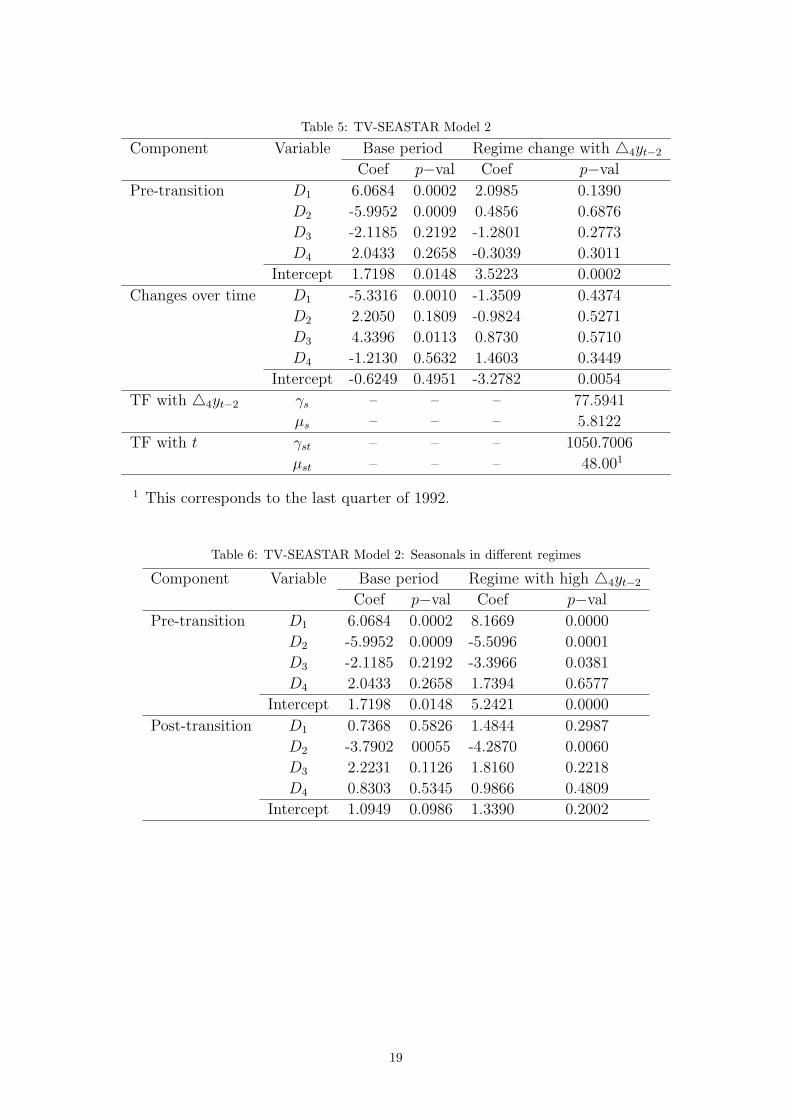
Table 5: TV-SEASTAR Model 2

Component Variable Base period Regime change with 44yt−2

Coef p−val Coef p−val

Pre-transition D1 6.0684 0.0002 2.0985 0.1390

D2 -5.9952 0.0009 0.4856 0.6876

D3 -2.1185 0.2192 -1.2801 0.2773

D4 2.0433 0.2658 -0.3039 0.3011

Intercept 1.7198 0.0148 3.5223 0.0002

Changes over time D1 -5.3316 0.0010 -1.3509 0.4374

D2 2.2050 0.1809 -0.9824 0.5271

D3 4.3396 0.0113 0.8730 0.5710

D4 -1.2130 0.5632 1.4603 0.3449

Intercept -0.6249 0.4951 -3.2782 0.0054

TF with 44yt−2 γs – – – 77.5941

µs – – – 5.8122

TF with t γst – – – 1050.7006

µst – – – 48.001

1 This corresponds to the last quarter of 1992.

Table 6: TV-SEASTAR Model 2: Seasonals in different regimes

Component Variable Base period Regime with high 44yt−2

Coef p−val Coef p−val

Pre-transition D1 6.0684 0.0002 8.1669 0.0000

D2 -5.9952 0.0009 -5.5096 0.0001

D3 -2.1185 0.2192 -3.3966 0.0381

D4 2.0433 0.2658 1.7394 0.6577

Intercept 1.7198 0.0148 5.2421 0.0000

Post-transition D1 0.7368 0.5826 1.4844 0.2987

D2 -3.7902 00055 -4.2870 0.0060

D3 2.2231 0.1126 1.8160 0.2218

D4 0.8303 0.5345 0.9866 0.4809

Intercept 1.0949 0.0986 1.3390 0.2002

19

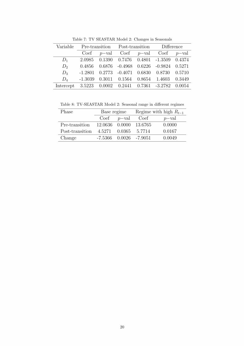
Table 7: TV SEASTAR Model 2: Changes in Seasonals

Variable Pre-transition Post-transition Difference

Coef p−val Coef p−val Coef p−val

D1 2.0985 0.1390 0.7476 0.4801 -1.3509 0.4374

D2 0.4856 0.6876 -0.4968 0.6226 -0.9824 0.5271

D3 -1.2801 0.2773 -0.4071 0.6830 0.8730 0.5710

D4 -1.3039 0.3011 0.1564 0.8654 1.4603 0.3449

Intercept 3.5223 0.0002 0.2441 0.7361 -3.2782 0.0054

Table 8: TV-SEASTAR Model 2: Seasonal range in different regimes

Phase Base regime Regime with high Rt−1

Coef p−val Coef p−val

Pre-transition 12.0636 0.0000 13.6765 0.0000

Post-transition 4.5271 0.0365 5.7714 0.0167

Change -7.5366 0.0026 -7.9051 0.0049

20

Fig. 1

Q(1) Q(2) Q(3) Q(4)

Seasonals in IIP

1981 1983 1985 1987 1989 1991 1993 1995 1997 1999 2001 2003-20

-15

-10

-5

0

5

10

15

Notes:

1. The value for a given quarter represents deviation of sample mean of first differenced log IIP in that quarter from average of such sample means for all quarters during that period, thus giving the quarterly growth rate of IIP relative to the average quarterly growth rate over the year.

2. These were calculated by running the rolling regression of first differenced log IIP on four seasonal dummies and then taking deviation of each quarter from the average of the four coefficients. The window size was 16 (implying that each coefficient gives average growth rate of first differenced log IIP in that period for four years) and the points on the time axis correspond to the first point in the window. Thus, for instance, a value shown here against 1991q1 is for the period 1991q1-1994q4.

21

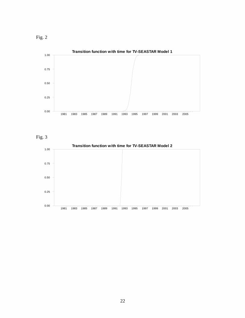
Fig. 2

Transition function with time for TV-SEASTAR Model 1

1981 1983 1985 1987 1989 1991 1993 1995 1997 1999 2001 2003 20050.00

0.25

0.50

0.75

1.00 Fig. 3

Transition function with time for TV-SEASTAR Model 2

1981 1983 1985 1987 1989 1991 1993 1995 1997 1999 2001 2003 20050.00

0.25

0.50

0.75

1.00

22