MODELLING THE TEMPERATURE,MATURITY AND MOISTURE CONTENT IN A

DRYING CONCRETE BLOCK

Workshop participants: Jaco Bruyns, Jean Charpin, Corrie Lock, 0Daniel Makinde, Peter Y Mhone, Gift Muchatibaya, Tim Myers, NneomaOgbonna, Astri Sjoberg and Samuel M Tshehla

In this paper we continue work from a previous Study Group in devel-oping a model for the maturation of concrete. The model requiresequations describing the temperature, moisture content and matu-rity (or amount of cement that has reacted with the water). Non-dimensionalisation is used to simplify the model and provide simpleanalytical solutions which are valid for early time maturation. A nu-merical scheme is also developed and simulations carried out for mat-uration over one day and then two months. For the longer simulationwe also investigate the effect of building the block in a single pour ortwo stages.

When cement is mixed with water to form concrete an exothermic reactionoccurs. The heat from the reaction leads to thermal expansion of the con-crete. When the concrete cools down it will contract and induce a stress inthe material. If the stress is sufficientlylarge it can lead to cracking which

"Department of Mathematics and Applied Mathematics, University of CapeTown, Rondebosch 7701, South Africa. e-mail: jcharpin@maths.uct.ac.za.my-ers@maths.uct.ac.za

tDepartment of Applied Mathematics, Auckland Park campus, University of Johan-nesburg, P.O. Box 524, Auckland Park, 2006, South Africa. e-mail: asjoberg@uj.ac.za

iSchool of Civil and Environmental Engineering, University ofthe Witwatersrand, Wits2050, Johannesburg, South Africa. e-mail: Yunnus.Ballim@wits.ac.za

obviously impairs the quality of the structure. With small concrete sections,surface cooling can quickly remove the heat and the resultant stresses willnot be large. With large sections of concrete the temperature increase canbe high, the surface cooling is slow and over long time periods very highstresses can build up. For this reason large concrete structures, such asdams, are built sequentially. New layers are only added when the earlierones have cooled down and contracted sufficiently.

The build up of heat in a concrete block is caused by the concrete reactingwith water. Therefore in order to model the temperature evolution in aconcrete block it is necessary to describe the water content (the moisture)as well as the proportion of cement available to react with the water (this ismeasured in terms of maturity). Knowledge of these variables is importantfor other reasons as well. If the water is used up before all the cement hasreacted the maturing process will end prematurely and the concrete doesnot reach its optimal strength. Pavlik et al [1] point out that the mouldaround a concrete block can only be removed after the concrete has reacheda certain strength, which depends on the curing process. They go on todescribe a microwave technique for measuring water content as a meansof determining the concrete maturity. West & Holmes [2] investigate theproblem of damage to impervious concrete floor coverings. This problemarises because builders often do not wait for the concrete to cure properlybefore finishing the floor. Further, current tests to determine when thefloor can be finished only measure the concrete surface moisture content,neglecting the moisture further down in the block.

An understanding of the temperature, moisture content and maturityof concrete is therefore important in determining when to add new layersof concrete. It also helps determine the strength and possibility of crack-ing. At the first South African Mathematics in Industry Study Group 2004the problem of modelling the maturing of a concrete block was introducedby the Cement & Concrete Institute. The initial model developed duringthe meeting and subsequently is described in [3]. The task of the StudyGroup was to investigate analytical and numerical solutions of the systemof equations that model temperature, moisture content and maturity sub-ject to suitable boundary and initial conditions. In answer, in the presentreport we take the preliminary work of [3] and attempt to refine it, as well .as provide solutions for practical situations. The model equations of [3] aswell as our own refinements are discussed in Section 2. In Section 3 we writethe problem in non-dimensional form and identify small parameters. Thispermits some simplifications that are used in Section 4 to provide simpleanalytical solutions. In Section 5 we describe a numerical scheme to solve

the full system of equations. Results are presented for simulations over oneday and two months. We also consider the effect of adding a second concretelayer after one month. The notation and typical values of the constants aregiven in the nomenclature in Section 7.

8T 82T 8m(1)Pccc7!ii K, 8x2 + 'Y7ft '

8m J.L(1 - m)()e-E/RT , (2)=8t8e ~(D(e)8e)_ 8m (3)8t 8x 8x T) 8t '

where T, m and e denote the temperature, maturity and moisture of theconcrete respectively. All coefficients,with the exception of the diffusion,D(B), are constant. In [3] it was suggested that the diffusion coefficientD rv e36 but then e was set to 1 throughout the slab and so D becameconstant. Equation (1) is the standard heat equation with a source termdue to the chemical reaction. The maturity is a measure of the amount ofcement that has reacted with the water. The maturity variation is governedby an Arrhenius type equation, namely equation (2). Finally, the watercontent or moisture must also satisfy a diffusion equation. The sink term,-rJmt in equation (3), indicates that water is used up in the reaction. Thenotation is defined in the nomenclature, Section 7.

The initial and boundary conditions used in [3]were

which reflects the daily and monthly temperature variation. Evaporationwas accounted for by

08 = aT = o.ax axAs the basis of our work we will use the above equations (1- 3). However,

it should be noted that these equations were part of a preliminary study andas such involved certain simplifications that may be improved upon in thisfollow-on study. The modifications are as follows:

1. The final term of equation (1), namely ,mt where, is constant, shouldread Qt, since it represents the heat generation. It may be expressed interms of the maturity by Qt = Qmmt, hence in the previous work, rv

Qm. A typical form for Qm is shown by curve (a) in Figure 1, where thedotted line (b) represents the constant approximation. Clearly curve(a) is far from constant and so we will replace the constant value for'Ywith a curve of the form

2'Y = Qm = Ame-am

If the maximum value of Qm occurs at (mx, Qx) then a = 112m; andA = Qxvelmx.

2. The surface temperature boundary condition, equation (4), basicallystates that the temperature is known (and matches the ambient tem-perature). This is a reasonable first approximation, however,in generala cooling condition will provide a more accurate model. This was in-vestigated in [4] for exactly this problem. In that report it was shownthat the concrete surface temperature lags behind the air temperatureand is also greatly affected by the sun. This result agrees with ex-perimental measurements. A more reasonable boundary condition istherefore

where Qs represents the solar radiation and Ta the ambient temper-ature. Both can be functions of time and, in particular, if we let Tabe defined by the right hand side of equation (4) then we correctlyinclude the ambient temperature variation. Equation (4) is valid overlong time periods. Since our interest is in shorter time-scales, in thenumerical solutions of Section 5 wewill neglect the monthly variation.

3. The bottom of any block, which is placed on the ground or anotherblock, will be subject to very different conditions to the top, which isexposed to the air. Hence symmetry is not appropriate. Instead weassume the bottom is insulated. This could represent a block on soilor some other relatively poor conductor. However, the block could beon top of rock which is a good conductor, and so a different conditionwill be required. In the absence of information we choose the insulatedcondition.

4. The diffusion coefficient in equation (3) may vary with moisture. Thevariation is discussed by West et al [2]. Their results show a maximumvariation in the range [1,5] x 10-9m2/s (provided you interpret theirunsound axes correctly). They also provide a closed form algebraicexpression for the variation. A simpler representation is given by

where Dm rv 2 x lO-9m2/s, a I'V 0.05, Om rv 0.8 and a '" 20. Wewill take D as constant D rv 2 x 10-9m2/s when calculating analyticalresults. In the numerical results we will allow for diffusion variation.The boundary condition (5) is modified to

-D(O(L,t)) 8o~x,t)1 =e(Oa-O(L,t)).x x=L

West et al [2]also discuss the evaporation rate e which occurs in equa-tion (5). This rate actually decreases slowlywith time. However, thedecrease, in a controlled room, is around 5% after 50 days. In thelaboratory the decrease is around 17% after 90 days, hence we willtake it as constant, e rv 1.8 X 10-9 m/s.

A Xx= -

LA DD=-Dm

where T a is the average ambient temperature and T is the time-scale. Thematurity is a fraction between 0 and 1 and is already non-dimensional. Weimmediately drop the hat notation.

The non-dimensional equations governing the problem are:

8Tat

omatof)at

= al :x (~~) + a2Qm a; ,= ag (1 - m )8e1/(a4+asT) ,

o ( af)) oma6- D(f))- - a7-ax ax at '

/'i,T

a1=-L2 'PcCc

a3 = T/-Lf)i ,

TDm0:6=0'

0:1 7.36 x 10 -[) 0:2 21.26 0:3 10000:4 -0.07 0:5 -6 X 10-3 0:6 2 X 10-70:7 1.25 {32 -10.94 {33 -2.7

• At t = 0, temperature, maturity and moisture are constant throughoutthe layer

8T1 =0ox x=o 'ael -0ax x=o - .

(.? __ QsL + H L (Ti - Ta)1-'1 - ",6.T '

HLf32 = -- ,'"

L-e{33 = -- .Dm

Typical values for O:i and {3i are given in Table 1. If the ambienttemperature is taken as constant (for example if we are interested insolutions over a short period) then Ta = 1, otherwise {31 = (31(t).Typical values for other parameters are given with the definitions inthe nomenclature section.

Consider the parameter values shown in Table 1. The diffusion parameters0:1 and 0:6 are both small. Physically this means that diffusionis, in general,slow and consequently the x variation of T and e is negligible throughoutmost of the domain. Neglecting the x derivatives means we are unableto satisfy the boundary conditions. Since we choose Tx = ex = 0 at thebottom an x independent solution is automatically satisfied there. However,

to satisfy the upper conditions, a boundary layer must be present in thevicinity of x = l.

A standard boundary layer scaling indicates the appropriate layer thick-nesses are given by LT = J<il and Lm = .jCi6 respectively. Using the valuesgiven in Table 1 we expect LT >:::::: lcm, Lm >:::::: 0.5mm. In our subsequentnumerical solutions a boundary layer of around 2cm may be observed onsome of the maturity curves (see the 35, 40 and 60 day curves on Figure 10for example). However, in general, the fluctuations in the ambient temper-ature prevents us from seeing the boundary layer. We also see no benefitin carrying out the boundary layer analysis since when we rescale in theboundary layers we end up retaining all terms in the governing equations,even the original boundary conditions hold. Hence we may as well solve theoriginal system in the first place. Instead we will now simply look at thesolution in the bulk.

Neglecting the small diffusion terms in equations (10) and (12), ourtemperature and moisture equations are

aT amfit = cxzQm at ' aB am

-=-CX7-at at .The second equation in (18) integrates immediately to determine the mois-ture in terms of the maturity

B = 1-cx7m,

so the moisture decreases linearly with maturity.With the definition of Qm given by equation (13) we find

T = cxzm; (1- e-m2/(zm;)) .

We could now replace T and B in the maturity equation (11), resultingin a first order differential equation to solve numerically, and hence deter-mine the bulk solution for m. An alternative approach is to note that theexponential term in the maturity equation (11) contains CX4 + (X,5T. SinceCX4 '" lOcx5 we may neglect the term cx5T, provided T remains small. Hencea reasonable approximation is to model maturity with

am /at = cx3(1 - m)Be1U4 • (21)

Substituting for e from equation (19) into equation (21) leads to a first orderseparable equation for m,

am /at = cx3(1- m)(l - cx7m)e1 U4

1- e( o<ae1/<>4)(a7-1)tm-

- 1- CY7e(o<ae1/<>4)(0<7-1)t

(CY3e1/0<4) tm-------- 1+ (CY3e1/0<4)t .

1- e(o<ae1/ae4)(0<7-1)te = 1- CY7--------1-CY7e(o<ael/<>4)(0<7-1)t

The variation of m, e and T are shown in Figure 2. The time-scale T =WOOsand the temperature scale .6.T = 25K, so this simulation which runsto t ~ 2600 corresponds to 30 days. The maturity increases monotonically,

tending to the asymptote 1/C1-7 = 0.8. After 30 days it is still well belowthis value at m rv 0.57. The moisture e decreases as m increases. Thetemperature also increases towards an asymptote but is not close to theasymptote after 30 days. The temperature rise is rather high. With thescale of 25K we see that the rise is around 125K over 30 days. This canbe attributed to the neglect of the cooling condition at the free surface.There is no mechanism for heat to escape and consequently it builds upvery rapidly. This has consequences in the neglecting of the term C1-5T inthe maturity equation. Since T builds up rapidly this approximation canonly hold for short time periods, .of the order of days. We show this insubsequent graphs in the numerical section. In particular, in Figure 7, weshow that the maturity approximation is excellent after 2 days with only asmall difference at the free surface. After 10 days there is a 15%differencebetween analytical and numerical bulk solutions.

In general, of the three curves we expect the temperature to be the leastrealistic. The maturity satisfies a first order ordinary differential equation,and we satisfy the initial condition. The temperature and moisture bothsatisfy diffusionequations, however,we neglect the diffusion terms. In bothcases we satisfy the initial condition and the boundary condition at x = 0,but cannot satisfy the surface condition. However,the coefficient C1-6 « C1-1

and so we expect the largest boundary layer effect with the temperatureequation. Hence we expect m to give the best approximation, then e andfinally T is probably the worst. We will investigate this further when wesolve the full equations numerically.

From these results we can make a statement about C1-7. Firstly, if C1-7 > 1then as t ---t 00 the exponential terms dominate in equation (23) and m ---t

1/ a7. Hence the maturity can never reach unity. If a7 < 1 then as t ---t 00

the exponential terms decay and the maturity m ---t 1. If C1-7 = 1 we alsofind m ---t 1. Experimental results showthat the maturity typically increasesto a maximum of around m = 0.8. This motivates our choice a7 = 1.25.Practically by taking a number of maturity measurements over time, wecould estimate all the parameters a3, a4 and a7 in the maturity equation.

The system will now be solvednumerically, using a standard finite differencemethod. The three parameters T, m and e are calculated on equally spacedpoints numbered from 0 to nx, including the boundaries, separated by the

space step ~x = l/nx. The simulation time tm is divided in nt time stepsdenoted ~t = tm/nt. The temperature, maturity and moisture at x = i~xand t = k~t are denoted Tik, mf, Of respectively.

To slightly simplify the system, the equations may be rewritten:

8T cPT= al 8x2 + a2a3Qm(m)(1 - m)Oe1/(a4+asT) , (27)

8t8m a3(1- m)Oe1/(a4+asT) , (28)=8t8e a6!- (D(e) 8e) - lY307(1- m)Oe1/(a4+asT). (29)=8t 8x 8x

Equations (27) and (29) are diffusion equations with respectively a sourceand a sink term. They involve second order space derivatives that are keyin the stability of the numerical scheme. They will be discretised with apartially implicit scheme:

• The space derivatives are discretised using an implicit method to guar-antee good stability of the numerical scheme,

• The two parameters, D(e) and Qm(m), and the source and sink termsare discretised with an explicit method. In theory, they could also bediscretised with an implicit method but the resolution of the systemwould become too time consuming.

Equation (28) does not involve any space derivative and may be discretisedusing an explicit method.

Using the standard finite volume method leads to the following differenceequations:

[2al~t] T~+l

~x2 ~-1

= Tik + o2a3ri~t .

At the boundary x = 0 we apply Tx = 0 from equation (15) and so impose

[2al~t] k+l [2al~t] k+l k1+ ~x2 To - ~x2 T1 = To + a2a3ro~t .

Tk + 2al;Jl~tnx ~X

+a2a3fn~t ,

fo _ ~X [(1- mo)Qm(mo)eoe1/(a4+a5To)

+(1- ml/2)Qm(ml/2)el/2el/(a4+a5Tl/2)] ,

fi - ~x [(1- mi_l/2)Qm(mi_l/2)ei_l/2el/(a4+a5Ti-l/2)

+(1- mi+l/2)Qm(mi+l/2)ei+l/2e1f(a4+a5Ti+l/2)] ,

1$ i $ nx -1 ,

= ~x [(1- mnx_l/2)Qm(mnxl/2)enx_l/2e1f(a4+a5Tnx-l/2)

+(1- mnx)Qm(mnx)enxel/(a4+a5Tnx)] ,

mi + mi+l e ei + ei+lmHl/2 = 2 i+l/2 = 2

Ao = ~x [(1 - mo)Ooe1/(0<4+oSTO) + (1 - ml/2)el/2e1/( 04+osT1/2)]

Ai = ~x [(1- m· )0. e1/(04+o<sTi-1/2)2 t-l/2 t-l/2

+(1- mi+l/2)ei+l/2el/(a4+osTi+l/2)] ,1:S i:S nx -1 ,

= ~x [(1_ m )0 el/(a4+0STnx-l/2)4 nx-l/2 nx-1/2

+(1- mnx)enxel/(04+osTnx)]

Equation (33) leads directly to the maturity at time t = (k + l)~t.Equations (31-32) and (35-36) form two tri-diagonal systems of nx linearequations each of nx unknowns, namely the values of T and 0 at time t =(k+ l)~t. These two systems may be solved easily with an LU factorisationfor example.

The numerical scheme is now complete so we move on to presenting theresults.

The solutions of the governing equations will be described in three differ-ent situations. Firstly the evolution of the variables will be studied duringa single day, to evaluate the influence of the varying ambient conditions.Secondly, a two month simulation will be carried out, where the concrete

layer is built in a single stage. Finally, another two month simulation willbe studied where the block is built in two stages, with the second stagebeing added after one month. The values of the constants used for all thesesimulations may be found in Table 1.

Temperature variation and sun exposure is represented as follows:

• The minimum temperature Tmin = 288K occurs one hour before sun-rise.

• Temperature variation during the day is modelled with a cosine func-tion.

Using the definition given in Equation (17), the parameter /31 may then beexpressed as:

/31 = 43.8f(t) - 3.28cos [~~ (t - 5.5)] ,

where t represents the time of the day in hours and the function f(t) definesthe daylight hours, when solar radiation plays a role,

f(t) = {1 if 6.5.::;t ::;19.5 ,o otherwIse.

5.2.1 One day simulation

Figure 3 shows the evolution of the temperature inside the concrete layerduring the first 24 hours. Only the top of the layer is shown on the picture,for the heights 0.6 ::; x ::; 1. The temperature does not vary in space forx ~ 0.6, so this part was excluded to make the picture clearer.

The initial temperature of the layer is T = O. Temperature profilescorresponding to times t = 15.00,19.00,20.00,0.00(+1), 6.00(+1), 7.00(+1),12.00(+ 1) are shown in Figure 3. Two heating effects can be observed. Thechemical reaction leads to a slow release of energy which acts to increasethe temperature throughout the block. We can see at x = 0.6 that thereis a very small rise in the temperature. The boundary condition Tx = 0,imposed at x = 0, prevents energy from leaving at that boundary. Hence,

1.6

1.4

1.2OJl-l 1;:l.IJn:ll-l 0.8OJ§' 0.6OJH

0.4

0.2

even though the hydration reaction is slow, the temperature must slowlyincrease inside the block.

In the vicinity of x = 1 we see the effect of the ambient temperature onthe block. During day time, between 06:30 and 19:30 in the present case, theradiation of the sun heats the top of the layer very significantly. This causesthe sudden increase of temperature at the surface. This effect is balancedby the influence of the ambient temperature. During the day, the ambienttemperature is assumed to vary between Tmin = 15°0 and Tmax = 30°0 indimensional form, corresponding to Tmin = -0.3 and Tmax = 0.3 in non-dimensional form. The surface temperature is well above T = 0.3 from thefirst hour so the ambient temperature cools the surface down. This effectis hard to notice during day time, but as soon as solar radiation stops, thetemperature at x = 1 drops significantly. After 30 minutes without sun,at 20:00, the non-dimensional drop in temperature reaches b..T = 0.4. Justbefore sunrise, at 06:00, the surface temperature has dropped to T = 0.3from T ~ 1.6 the previous day at 19:00. When the sun rises again, thetemperature makes a significant jump and at the end of the first 24 hours,it has reached T = 1.6, slightly above the maximum temperature observedthe previous day.

The heat gained at the surface slowlydiffusesthrough the concrete layer.The variations at the surface of the layer only affect the temperature above

x = 0.9 at first. Progressively,the effectsmay be seen up to x = 0.75 afterone day. However, during the first day, most of the heat inside the layer isreleased by the chemical reaction and heat diffusion is mainly observed atthe top of the layer.

0.15

>t,iJ'';l-I 0.1::s,iJnj

::E:

0.05

/i;;;

t=15.00 l,/

I./ ,I

...__.__._._. ._. ._._.._!:::nQ.Q_L+..1L.-. -._-._.. _.----,/' /./';

_.............................................. J..=.:=..Q,QQ.(±J.L _ --.. ". ./.... . J:=:J~9.9. ,------------------~------------ --------------------- ----------------- ------------------_ .•~a

a

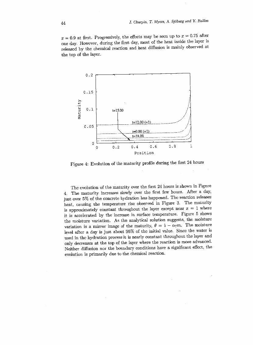
The evolution of the maturity over the first 24 hours is shown in Figure4. The maturity increases slowly over the first few hours. After a day,just over 5% of the concrete hydration has happened. The reaction releasesheat, causing the temperature rise observed in Figure 3. The maturityis approximately constant throughout the layer except near x = 1 whereit is accelerated by the increase in surface temperature. Figure 5 showsthe moisture variation. As the analytical solution suggests, the moisturevariation is a mirror image of the maturity, () = 1 - CY.7m. The moisturelevel after a day is just about 95% of the initial value. Since the water isused in the hydration processit is nearly constant throughout the layer andonly decreases at the top of the layer where the reaction is more advanced.Neither diffusion nor the boundary conditions have a significant effect, theevolution is primarily due to the chemicalreaction.

1

0.980.960.94

(1) 0.92l-l;:l+,l 0.9III•.-10 0.88:8

0.860.840.82

0.80

The evolution is now studied on a much longer term. The daily variationsare still taken into account in the simulation but for comparison purposes,the variables are always plotted at midday in the followingtwo sections.

The variation of the maturity over the first two months may be seen inFigure 6. The trend observed in Figure 4 that the maturity is approximatelyconstant through the bulk can still be seen, but as t increases the increasenear x = 1 diffuses through the layer. After 60 days the maturity shows avery slight linear increase from x = 0 to around x = 0.98, followedby a smalldecrease. The maturity is everywhere slightly below its maximum possiblevalue of 0.8. In Figure 7 we compare the numerical and analytical solutionsfor maturity after 2 and 10 days. After 2 days, the constant analytical solu-tion and the numerical solution are nearly equal over most of the layer, theyonly differ near x = 1 where the external energy has accelerated the reactionin the numerical solution. After 10 days, a lot of heat has been released inthe layer due to the hydration reaction. The numerical solution also feelstheexternal energy input and this extra energy has diffused through the block.The result is that the analytical solution differs from the numerical one byabout 15% in the bulk and the correspondence deteriorates as the top is

0.9 ,-------r------,,-----,------,----,0.8 ~~~?~~__. ._------. --' -----. -. ---.--------'.0.7

0.6>.+J.,-1 0.5~ --_!~-~~~----------+J 0.4~

0.3

0.2

0.1

,////-'

_...-'5 days -- ..- ..

~ H_ __ _ ----- ..-

....................

.....2 ~x.~ . .. . .---------------------------------------------------------------------------------------_ ••.-.,,/

1 dav

0.2

approached. This result is in agreement with our earlier statement that theanalytical solution will only hold for early times. The moisture evolution is

t' 0.6...•~'-'~ 0.4

shown in Figure 8. The moisture slowly decreases throughout the block, butthe decrease is most rapid near x = 1 where water is lost to the hydrationreaction and evaporation. After 60 days we can see that for x < 0.8 thereis a small amount of water remaining and so the hydration can continuefor some time longer. For x > 0.8 the water has been used up and the

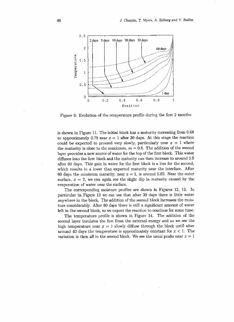
reaction can therefore only continue if water can diffuse in. Since diffusionis very slow this will slow the reaction down significantly. Hence, after 60days both the maturity and moisture have almost reached their final limits.The temperature evolution, shown in Figure 9, behaves in a very different

lr----..,--:-;----r---,-----.-----,o . 9 ~_~~~~~_~::~~~::~~-_::~~_J~~i~_:~~~_-_::~~_-::~~~::~~_~~::~.-.:::~.:::~~.:::~~.::::::.~-----\

.............\...

•.•.•.•.•.•.•.•.•.•.•.,

manner. Temperature increase is due to the hydration reaction and energygains or loss (at night) at the surface x = 1. The insulation condition atx = 0 prevents any heat loss there. Heat diffusion in concrete is very slow.The diffusion coefficient Dc = KI PcCc f'J lQ-6m2 Is. Consequently we see aslow temperature rise near x = O. Near x = 1 the temperature remainshigh at the boundary and this can be seen to diffusethrough the layer. As tincreases diffusionallowsmuch of this energy to be spread through the layer,which will tend towards the average daily temperature. There will alwaysbe a boundary layer near x = 1 that reflects the daily variation, which doesnot have time to diffuse far.

5.2.3 Two month simulation with two layers

Finally, we investigate the effect of adding a second layer to the first after30 days. We begin by running the simulation for a single block for 30 days.We then place an identical block on top, with the same initial conditions asthe original block.

The maturity evolution is shown in Figure 10. A closeup of the interface

2.5

2<lJH;::l 1.5.IJmH<lJ

~ 1<lJH

0.5

2 days 5 days 10 days 20 days 30 days !.:~

./:~60 days ,Ii/if

..- /.._..._.._._...._ .... ,I

-.:~~::-.:::::-.:~:::-.:_:.:-.:~:::-.::::::.~::::.:.:::.:::::.~:::-.:::::::.~::~~:::~~:~~:~~:·.-_.·/;'~ayoo

is shown in Figure 11. The initial block has a maturity increasing from 0.68to approximately 0.78 near x = 1 after 30 days. At this stage the reactioncould be expected to proceed very slowly, particularly near x = 1 wherethe maturity is close to the maximum, m = 0.8. The addition of the secondlayer provides a new sourceofwater for the top of the first block. This waterdiffuses into the first block and the maturity can then increase to around 0.9after 60 days. This gain in water for the first block is a loss for the second,which results in a lower than expected maturity near the interface. After60 days the minimum maturity, near x = 1, is around 0.62. Near the outersurface, x = 2, we can again see the slight dip in maturity caused by theevaporation of water near the surface.

The corresponding moisture profiles are shown in Figures 12, 13. Inparticular in Figure 13 we can see that after 30 days there is little wateranywhere in the block. The addition of the second block increases the mois-ture considerably. After 60 days there is still a significant amount of waterleft in the second block, so weexpect the reaction to continue for some time.

The temperature profile is shown in Figure 14. The addition of thesecond layer insulates the first from the external energy and so we see thehigh temperature near x = 1 slowly diffuse through the block until afteraround 40 days the temperature is approximately constant for x < 1. Thevariation is then all in the second block. We see the usual peaks near x = 1

1

0.90.80.7

t' 0.6'rl

~ 0.5..,~ 0.4

0.30.20.1

oo

Figure 10: Evolution of the maturity profile during the second month of atwo layer simulation

1

0.90.80.7>,..,0.6·rl

l..l;:J.., 0.5III:;:

0.40.30.2

32 days31 days

30 days

I1·········---------- --------------------------L. • •• _

due to the high midday temperatures. The central part of the second blockis originally cool but rapidly heats up since it is heated from both sides. Atthe end of the simulation the temperature profile shows no indication of thetwo stage building.

10.90.80.7

Q> 0.6I-i::l+J 0.5Ul•.-10 0.4~

0.30.20.1

Figure 12: Evolution of the moisture profile during the second month of atwo layer simulation

0.90.80.70.6

Q>I-i::l 0.5

+JUl

•.-1 0.40~ 0.3

0.20.1

o0.980.9850.990.995

t=31 day~. . _

,//-·······--··--~·~;~~~.~~:.S.___......../ ...-

I i

f/i t=35_~a.~~

L//--------.. t=40 da~~ _

1=30 days J'l --------------I ••• -

tj.-'-'..:,1 t 60 d= - - -~~~.-_..--

. ---;;~~-.,..~~/. - - - . - ~- --

The main output of this work is the numerical scheme that can model theevolution of maturity, moisture and temperature of a concrete block throughtime. Results were presented for both short and long times.

2.5

2lI>hi;:l 1.5....,ctlhilI>0.SlI>

[,-<

0.5

00

Figure 14: Evolution of the temperature profile during the second month ofa two layer simulation

A number of interesting features were observed in the calculations. Forshort times, of the order of days, the maturity increases most rapidly nearthe free surface. However, over a long period this surface will be the leastmature, due to the fact that water evaporates there and so is not availablefor the reaction. Of course over even longer time periods it is possible thatwater from the atmosphere could permit the reaction to slowly continue.When a second layer is added to the first then water can diffuse from theupper layer to the lower one. This results in the top of the lower layerbecoming more mature than expected. The loss of water at the bottom ofthe upper layer leads to a decrease in maturity there. The bulk temperatureslowlyincreased throughout the simulations,.with only the top 20%reactingto the daily temperature fluctuations.

The analytical model showed good agreement with the numerical resultsfor small times, but the neglect of the temperature variation in the maturityequation and the cooling condition at the free surface prevented it frombeing applicable over long times.

The graphs of moisture content showedthat the free surface would al-ways have a lowerwater content than deeper down in the block. In the twomonth simulations there was significantlymore moisture away from the sur-face, at times around a factor 2. If the concrete surface is covered with animpermeable layer then when this extra water diffusesto the surface it could

easily bring the surface moisture above the specified limit for the applyingthe covering, leading to the damage described in [2].

The numerical and analytical temperature profiles highlighted perhapsthe main drawback of the model, namely the boundary condition at x = O.There we imposed no energy loss, which prevents any heat from leaving atthis boundary. The results showed that this led to rather large temperatureincreases, particularly for the analytical model. In future work it will clearlybe necessary to address this issue and presumably include some form ofcooling condition, dependent upon the material below the initial block.

Acknowledgements

All contributors would like to thank Prof Yunus Ballim for introducing theproblem and assisting in answering questions. T.G. Myers acknowledgessupport of this work under the National Research Foundation of South Africagrant number 2053289. J.P.F. Charpin acknowledges the support of theClaude Harris Foundation.

Cc Thermal capacity of concrete 880 J.kg-1·K-1e Evaporation rate 1.8 X 10-9 m·s-1m Maturity 0-1 NDmx Parameter for the hydration heat re- 0.15 ND

leaset Time sT Time scale 1000 sx Cartesian coordinate mDm Moisture diffusivity in concrete 2 x 10 -!l m2·s-TE Apparent activation energy of the 35 x 103 J

reactionH Heat transfer coefficient 5 J·K-1·m-2·s-1L Length scale 3 mQs Heat received at the surface -500 J -2-1·m ·sQx Parameter for the hydration heat re- 108 J·m-3

leaseR Gas constant 8.314 J·K-1T Non-dimensional temperature 0-1 NDTi Initial temperature 295.5 Kb.T Typical temperature jump in the 25 K

block'Y Heat release coefficient due to hy- J·m-3

dration"7 Stoichiometric ratio for the hydra- 0.625 ND

tion reaction() Moisture content , 0-1 ND()a Ambient moisture content 0.05 ND()i Initial moisture content 1 NDK, Heat diffusion coefficient 1.37 J·K-1·m-1·s-1fL Reaction rate 1 S-1Pc Density of concrete 2350 kg·m-3

[1] Pavlik, J., Tydlitat, V., Cerny, R., Klecka, T., Bouska, P. and Rov-nanikova, P. Application of a microwave impulse technique to the mea-surement of free water content in early hydration stages of cement paste.Cement & Concrete Research 33 (2003), 93-102.

[2] West, R.P., Holmes, N. Predicting moisture movement during the dry-ing of concrete floors using finite elements. Construction & BuildingMaterials 19 (2005), 674-681.

[3] Fowkes, N.D., Mambili Mamboundou, H., Makinde, a.D., Ballim, Y.and Patini, A. Maturity effects in concrete dams. Proc. Mathematicsin Industry Study Group South Africa 2004, University of the Witwa-tersrand, (2004), 59-67.

[4] Charpin, J.P.F., Myers, T.G., Fitt, A.D., Ballim, Y. and Patini, A.Modelling surface heat exchanges from a concrete block into the en-vironment. Proc. Mathematics in Industry Study Group South Africa2004, University of the Witwatersrand, (2004), 51-58.