models for eaf energy efficiency - steel times int · electric steelmaking 2 april 2017 1 electric...

ELECTRIC STEELMAKING 2

www.steeltimesint.com April 2017

ELECTRIC STEELMAKING1


THE EAF process is characterised by its flexibility in terms of production volume and raw materials. With recent market developments, the requirement to produce high-quality steels from lower-quality scrap, direct reduced iron (DRI), hot briquetted iron (HBI), hot metal (HM) and varying quality ferrous scrap blends at minimum conversion costs has increased. Specific electrical energy demand and electrode graphite consumption represent the most important contribution to conversion costs. Maximising yield from ferrous raw materials, oxygen, carbon, and alloys as well as minimising energy costs are top priority. At modern high productivity levels, even small process improvements generate considerable cost savings.

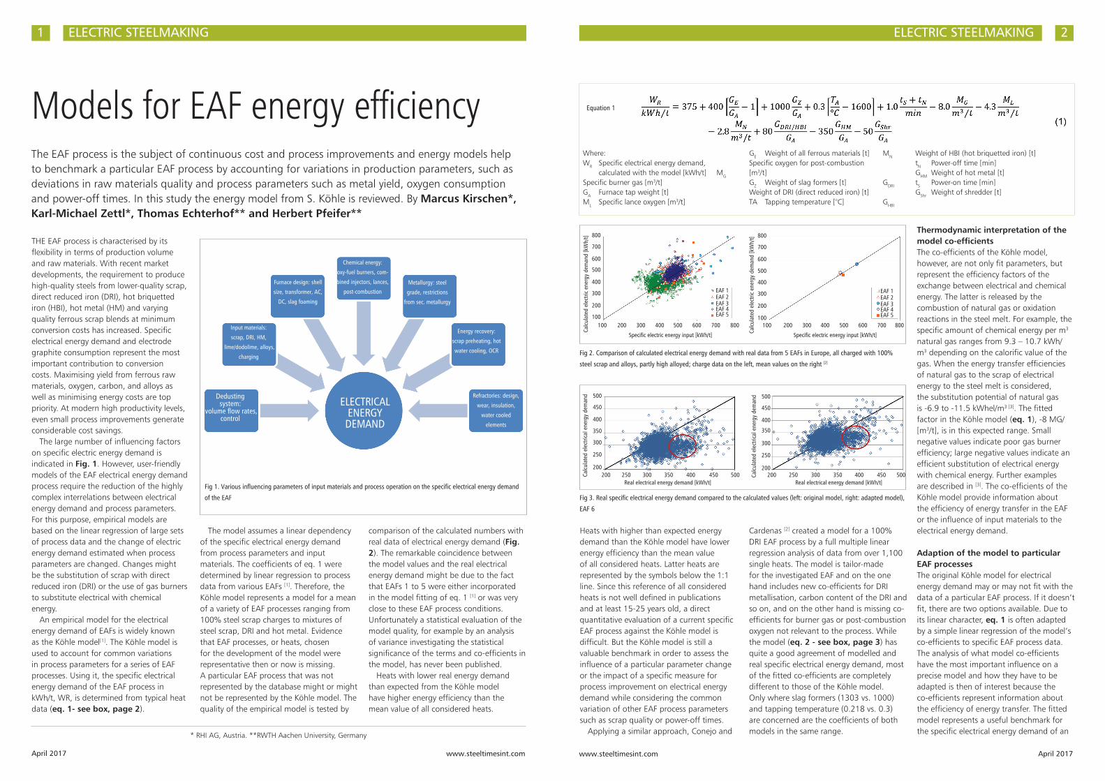
The large number of influencing factors on specific electric energy demand is indicated in Fig. 1. However, user-friendly models of the EAF electrical energy demand process require the reduction of the highly complex interrelations between electrical energy demand and process parameters. For this purpose, empirical models are based on the linear regression of large sets of process data and the change of electric energy demand estimated when process parameters are changed. Changes might be the substitution of scrap with direct reduced iron (DRI) or the use of gas burners to substitute electrical with chemical energy.

An empirical model for the electrical energy demand of EAFs is widely known as the Köhle model[1]. The Köhle model is used to account for common variations in process parameters for a series of EAF processes. Using it, the specific electrical energy demand of the EAF process in kWh/t, WR, is determined from typical heat data (eq. 1- see box, page 2).

* RHI AG, Austria. **RWTH Aachen University, Germany

Models for EAF energy efficiencyThe EAF process is the subject of continuous cost and process improvements and energy models help to benchmark a particular EAF process by accounting for variations in production parameters, such as deviations in raw materials quality and process parameters such as metal yield, oxygen consumption and power-off times. In this study the energy model from S. Köhle is reviewed. By Marcus Kirschen*, Karl-Michael Zettl*, Thomas Echterhof** and Herbert Pfeifer**

Fig 1. Various influencing parameters of input materials and process operation on the specific electrical energy demand

of the EAF

Dedusting system:

volume flow rates, control

Input materials:

scrap, DRI, HM,

lime/dodolime, alloys,

charging

Furnace design: shell

size, transformer, AC,

DC, slag foaming

ELECTRICAL ENERGY DEMAND

Chemical energy:

oxy-fuel burners, com-

bined injectors, lances,

post-combustion

Metallurgy: steel

grade, restrictions

from sec. metallurgy

Energy recovery:

scrap preheating, hot

water cooling, OCR

Refractories: design,

wear, insulation,

water cooled

elements

The model assumes a linear dependency of the specific electrical energy demand from process parameters and input materials. The coefficients of eq. 1 were determined by linear regression to process data from various EAFs [1]. Therefore, the Köhle model represents a model for a mean of a variety of EAF processes ranging from 100% steel scrap charges to mixtures of steel scrap, DRI and hot metal. Evidence that EAF processes, or heats, chosen for the development of the model were representative then or now is missing. A particular EAF process that was not represented by the database might or might not be represented by the Köhle model. The quality of the empirical model is tested by

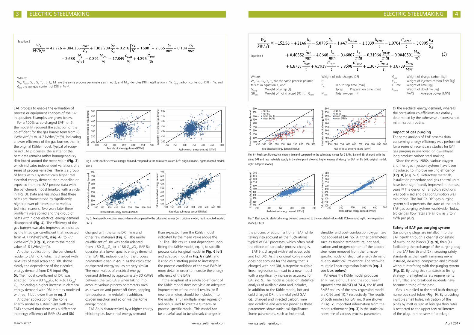
comparison of the calculated numbers with real data of electrical energy demand (Fig. 2). The remarkable coincidence between the model values and the real electrical energy demand might be due to the fact that EAFs 1 to 5 were either incorporated in the model fitting of eq. 1 [1] or was very close to these EAF process conditions. Unfortunately a statistical evaluation of the model quality, for example by an analysis of variance investigating the statistical significance of the terms and co-efficients in the model, has never been published.

Heats with lower real energy demand than expected from the Köhle model have higher energy efficiency than the mean value of all considered heats.

Heats with higher than expected energy demand than the Köhle model have lower energy efficiency than the mean value of all considered heats. Latter heats are represented by the symbols below the 1:1 line. Since this reference of all considered heats is not well defined in publications and at least 15-25 years old, a direct quantitative evaluation of a current specific EAF process against the Köhle model is difficult. But the Köhle model is still a valuable benchmark in order to assess the influence of a particular parameter change or the impact of a specific measure for process improvement on electrical energy demand while considering the common variation of other EAF process parameters such as scrap quality or power-off times.

Applying a similar approach, Conejo and

Cardenas [2] created a model for a 100% DRI EAF process by a full multiple linear regression analysis of data from over 1,100 single heats. The model is tailor-made for the investigated EAF and on the one hand includes new co-efficients for DRI metallisation, carbon content of the DRI and so on, and on the other hand is missing co-efficients for burner gas or post-combustion oxygen not relevant to the process. While the model (eq. 2 - see box, page 3) has quite a good agreement of modelled and real specific electrical energy demand, most of the fitted co-efficients are completely different to those of the Köhle model. Only where slag formers (1303 vs. 1000) and tapping temperature (0.218 vs. 0.3) are concerned are the coefficients of both models in the same range.

Where: WR Specific electrical energy demand, calculated with the model [kWh/t] MG Specific burner gas [m3/t]GA Furnace tap weight [t] ML Specific lance oxygen [m3/t]

GE Weight of all ferrous materials [t] MN Specific oxygen for post-combustion [m3/t]GZ Weight of slag formers [t] GDRI Weight of DRI (direct reduced iron) [t]TA Tapping temperature [°C] GHBI

Weight of HBI (hot briquetted iron) [t]tN Power-off time [min] GHM Weight of hot metal [t]tS Power-on time [min] GShr Weight of shredder [t]

Fig 2. Comparison of calculated electrical energy demand with real data from 5 EAFs in Europe, all charged with 100%

steel scrap and alloys, partly high alloyed; charge data on the left, mean values on the right [2]

Fig 3. Real specific electrical energy demand compared to the calculated values (left: original model, right: adapted model),

EAF 6

Equation 1

Thermodynamic interpretation of the model co-efficientsThe co-efficients of the Köhle model, however, are not only fit parameters, but represent the efficiency factors of the exchange between electrical and chemical energy. The latter is released by the combustion of natural gas or oxidation reactions in the steel melt. For example, the specific amount of chemical energy per m3 natural gas ranges from 9.3 – 10.7 kWh/m3 depending on the calorific value of the gas. When the energy transfer efficiencies of natural gas to the scrap of electrical energy to the steel melt is considered, the substitution potential of natural gas is -6.9 to -11.5 kWhel/m3 [3]. The fitted factor in the Köhle model (eq. 1), -8 MG/[m3/t], is in this expected range. Small negative values indicate poor gas burner efficiency; large negative values indicate an efficient substitution of electrical energy with chemical energy. Further examples are described in [3]. The co-efficients of the Köhle model provide information about the efficiency of energy transfer in the EAF or the influence of input materials to the electrical energy demand.

Adaption of the model to particular EAF processesThe original Köhle model for electrical energy demand may or may not fit with the data of a particular EAF process. If it doesn’t fit, there are two options available. Due to its linear character, eq. 1 is often adapted by a simple linear regression of the model’s co-efficients to specific EAF process data. The analysis of what model co-efficients have the most important influence on a precise model and how they have to be adapted is then of interest because the co-efficients represent information about the efficiency of energy transfer. The fitted model represents a useful benchmark for the specific electrical energy demand of an

800

500 500

800

700

450 450

700

600

400 400

600

500

350 350

500

400

300 300

400

300

250 250

300

200

200 200

200

100 100100

200 200

100200

250 250

200300

300 300

300400

350 350

400

Specific electric energy input [kWh/t]

Real electrical energy demand [kWh/t]Real electrical energy demand [kWh/t]

Specific electric energy input [kWh/t]

Calcu

late

d el

ectri

c en

ergy

dem

and

[kW

h/t]

Calcu

late

d el

ectri

cal e

nerg

y de

man

d

Calcu

late

d el

ectri

cal e

nerg

y de

man

dCa

lcula

ted

elec

tric

ener

gy d

eman

d [k

Wh/

t]

500

400 400

500600

450 450

600700

500 500

700800 800

EAF 1EAF 2EAF 3EAF 4

EAF 1EAF 2EAF 3EAF 4EAF 5 EAF 5


www.steeltimesint.com March 2017



EAF process to enable the evaluation of process or equipment changes of the EAF in question. Examples are given below.

For a 100% scrap-charged EAF no. 6, the model fit required the adaption of the co-efficient for the gas burner term from -8 kWhel/(m3/t) to -4.7 kWhel/(m3/t), indicating a lower efficiency of the gas burners than in the original Köhle model. Typical of scrap-based EAF processes, the scatter of the heat data remains rather homogeneously distributed around the mean value (Fig. 3) which indicates independent variations of a series of process variables. There is a group of heats with a systematically higher real electrical energy demand than modelled or expected from the EAF process data with the benchmark model (marked with a circle in Fig. 3). Data analysis shows that these heats are characterised by significantly higher power-off times due to various technical reasons. Two years later these problems were solved and the group of heats with higher electrical energy demand disappeared (Fig. 4). The efficiency of the gas burners was also improved as indicated by the fitted gas co-efficient that increased from -4.7 kWhel/(m3/t), (Fig. 4), to -7.1 kWhel/(m3/t) (Fig. 3), close to the model value of -8 kWhel/(m3/t).

Another application of the benchmark model to EAF no.7, which is charged with mixtures of steel scrap and DRI, shows clearly the dependence of the electrical energy demand from DRI input (Fig. 5). The model co-efficient of DRI was adapted from +80 GDRI/GA to +261 GDRI/GA, indicating a higher increase in electrical energy demand with DRI input as modelled with eq. 1 but lower than in eq. 2.

Another application of the Köhle energy model to a steel plant with two EAFs showed that there was a difference in energy efficiency of EAFs (8a and 8b)


EAF 7

Where: WR, GDRI, GA , GZ, TA , tS, tN, ML are the same process parameters as in eq.2, and MDRI denotes DRI metallisation in %, CDRI carbon content of DRI in %, and GDRI the gangue content of DRI in % [2].

Equation 2

charged with the same DRI, lime and other raw materials (Fig. 6). The model co-efficient of DRI was again adapted from +80 GDRI/GA to +186 GDRI/GA. EAF 8a operates at a lower specific energy demand than EAF 8b, independent of the process parameters given in eq. 1 as the calculated or expected energy values are very similar. The mean values of electrical energy demand differed by approximately 30 kWh/t between the two EAFs when taking into account various process parameters such as power-on and power-off times, tapping temperatures, lime/dololime addition, oxygen injection and so on via the Köhle energy model.

EAF 8b is characterised by a higher energy efficiency i.e. lower real energy demand

than expected from the Köhle model indicated by the mean value above the 1:1 line. This result is not dependent upon fitting the Köhle model, eq. 1, to specific process data (original model in Fig. 6 left and adapted model in Fig. 6 right) and is used as a starting point to investigate the process conditions of the two EAFs in more detail in order to increase the energy efficiency of the EAFs.

If the adaption of a single co-efficient of the Köhle model does not yield an adequate improvement of the model results, or if new parameters should be included into the model, a full multiple linear regression analysis is used to create a furnace- or process-specific model. This model can be a useful tool to benchmark changes in


EAF 6

500

600650700

600

650700

500

450

550 550

450

400

500 500

400

350

450 450

350

300

400 400

300

250

350 350

250

200

300 300

200

Calcu

late

d el

ectri

cal e

nerg

y de

man

dCa

lcula

ted

elec

trica

l ene

rgy

dem

and

Calcu

late

d el

ectri

cal e

nerg

y de

man

dCa

lcula

ted

elec

trica

l ene

rgy

dem

and

250200

300 300

300

350 350

350

400 400

Real electrical energy demand [kWh/t]

Real electrical energy demand [kWh/t] Real electrical energy demand [kWh/t]

400

450 450

450

550 550500 500

500

650 650700 700600 600

200 250 300 350Real electrical energy demand[kWh/t]

400 450 500

the process or equipment of an EAF, while taking into account all the fluctuations typical of EAF processes, which often mask the effects of particular process changes.

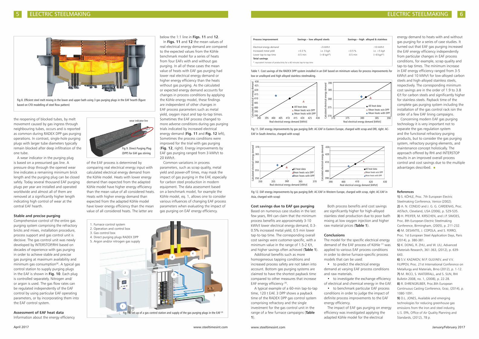
EAF 9 is charged with steel scrap, cold and hot DRI. As the original Köhle model does not account for the energy that is charged with hot DRI, a stepwise multiple linear regression can lead to a new model with a significantly increased accuracy for EAF no. 9. The model is based on statistical analysis of available data and includes, in addition to the Köhle model, hot and cold charged DRI, the metal yield GA/GE, charged and injected carbon, lime and dololime and average power as these parameters show statistical significance. Some parameters, such as hot metal,

shredder and post-combustion oxygen, are not applied at EAF no. 9. Other parameters, such as tapping temperature, hot heel, carbon and oxygen content of the tapped steel were removed from the furnace-specific model of electrical energy demand due to statistical irrelevance. The stepwise multiple linear regression leads to (eq. 3 see box below).

Whereas the Köhle model produces an R2 value of 0.31 and the root mean squared error (RMSE) of 74.4, the R2 and RMSE values of the new regression model are 0.96 and 10.7 respectively. The results of both models for EAF no. 9 are shown in Fig. 7. Important information from the model refinement (eq. 3) is the statistical relevance of various process parameters

to the electrical energy demand, whereas the correlation co-efficients are entirely determined by the otherwise unconstrained minimisation routine.

Impact of gas purgingThe same analysis of EAF process data concerning energy efficiency was performed for a series of recent case studies for EAF gas purging in unalloyed or low-alloyed long product carbon steel making.

Since the early 1980s, various oxygen and inert gas injection systems have been introduced to improve melting efficiency (Fig. 8) [e.g. 5-7]. Refractory materials, installation procedure and gas control units have been significantly improved in the past years.[8] The design of refractory solutions was optimised and gas consumption was minimised. The RADEX DPP gas purging system still represents the state-of-the-art in EAF gas purging systems worldwide. Today, typical gas flow rates are as low as 3 to 7 m3/h per plug.

Safety of EAF gas purging systemGas purging plugs are installed into the EAF hearth through a channel consisting of surrounding blocks (Fig. 9), thus (1) facilitating the exchange of the purging plug in the EAF hearth and (2) increasing safety standards as the hearth ramming mix is installed, de-aired, compacted and sintered without interfering with the purging system (Fig. 8). By using this standardised lining strategy, the highest safety requirements are fulfilled and break-out incidents have become a thing of the past.

Gas is supplied to the steel bath through numerous steel tubes (Fig. 9). By providing multiple small holes, infiltration of the pipes by melt or slag at low gas flow rates is restricted to the upper few millimetres of the plug. In rare cases of blockage

Fig. 6 - Real specific electrical energy demand compared to the calculated values for 2 EAFs, 8a and 8b, charged with the

same DRI and raw materials supply in the steel plant showing higher energy efficiency for EAF no. 8b (left: original model,

right: adapted model)

Fig 7. Real specific electrical energy demand compared to the calculated values (left: Köhle model, right: new regression

model), EAF 9

Where: WR, GE, GA, tS, tN are the same process parame-ters as in equation 1, and:GScrap Weight of Scrap [t]GHDRI Weight of hot charged DRI [t] GCDRI

Weight of cold charged DRI [t] tttt Tap-to-tap time [min] tprep Preparation time [min]MO2 Total oxygen [m³]

GchC Weight of charge carbon [kg]GinjC Weight of injected carbon fines [kg] GLime Weight of lime [kg]GDolo Weight of dololime [kg] PAVG Average power [MW]

Equation 3

500 500550 550600 600650 650700 700

450 450400 400350 350300 300250 250200 200

Calcu

late

d el

ectri

cal e

nerg

y de

man

d

Calcu

late

d el

ectri

cal e

nerg

y de

man

d

750 750800 800850 850900 900

700 700650 650600 600550 550500 500450 450

Calcu

late

d el

ectri

cal e

nerg

y de

man

d

Calcu

late

d el

ectri

cal e

nerg

y de

man

d

450 450500 500550 550


600 600700 700650 650800 800850 850900 900750 750

200 200300 300400 400Real electrical energy demand [kWh/t] Real electrical energy demand [kWh/t]

500 500600 600700 700

EAF 8a EAF 8aEAF 8b EAF 8bmean EAF8a mean EAF8amean EAF8b mean EAF8b


www.steeltimesint.com January/February 2017



the reopening of blocked tubes, by melt movement caused by gas ingress through neighbouring tubes, occurs and is reported as common during RADEX DPP gas purging operations. In contrast, single-hole purging plugs with larger tube diameters typically remain blocked after deep infiltration of the one tube.

A wear indicator in the purging plug is based on a pressurised gas line. A pressure drop through the opened wear line indicates a remaining minimum brick length and the purging plug can be closed safely. Today several thousand EAF purging plugs per year are installed and operated worldwide and almost all of them are removed at a significantly higher length indicating high control of wear at the central EAF hearth.

Stable and precise purgingComprehensive control of the entire gas purging system comprising the refractory bricks and mixes, installation procedure, process support and gas control unit is decisive. The gas control unit was newly developed by INTERSTOP/RHI based on decades of experience with gas purging in order to achieve stable and precise gas purging at maximum availability and minimum gas consumption[8]. A typical gas control station to supply purging plugs in the EAF is shown in Fig. 10. Each plug is controlled separately. Nitrogen and/or argon is used. The gas flow rates can be regulated independently of the EAF control by using particular EAF operating parameters, or by incorporating them into the EAF control system.

Assessment of EAF heat data Information about the energy efficiency

below the 1:1 line in Figs. 11 and 12.In Figs. 11 and 12 the mean values of

real electrical energy demand are compared to the expected values from the Köhle benchmark model for a series of heats from four EAFs with and without gas purging. In all of these cases the mean value of heats with EAF gas purging had lower real electrical energy demand or higher energy efficiency than the heats without gas purging. As the calculated or expected energy demand accounts for changes in process conditions by applying the Köhle energy model, these findings are independent of other changes in EAF process parameters such as metal yield, oxygen input and tap-to-tap times. Sometimes the EAF process changed to more adverse conditions during gas purging trials indicated by increased electrical energy demand (Fig. 11 and Fig. 12 left), Sometimes the process conditions were improved for the trial with gas purging (Fig. 12, right). Energy improvements by EAF gas purging ranged from 3 kWh/t to 20 kWh/t.

Common variations in process parameters, such as scrap quality, metal yield and power-off times, may mask the impact of gas purging in the EAF, especially for carbon steel production in modern equipment. The data assessment based on a benchmark model, for example the Köhle model, eq. 1, allows one to consider various influences of changing EAF process parameters when evaluating the impact of gas purging on EAF energy efficiency.

Fig 9. Direct Purging Plug

(DPP) for EAF gas stirring

wear indicator line

Fig 10. Set-up of a gas control station and supply of the gas purging plugs in the EAF [8]

of the EAF process is determined by comparing real electrical energy input with calculated electrical energy demand from the Köhle model. Heats with lower energy demand than expected from the adapted Köhle model have higher energy efficiency than the mean value of all considered heats. Heats with higher energy demand than expected from the adapted Köhle model have lower energy efficiency than the mean value of all considered heats. The latter are

Fig 8. Efficient steel melt mixing in the lower and upper bath using 3 gas purging plugs in the EAF hearth (figure

based on CFD modelling of steel flow pattern)

1. Furnace control system2. Operation and control box3. Gas control box4. Direct purging plugs RADEX DPP5. Argon and/or nitrogen gas supply

4

32

1

5

4

Cost savings due to EAF gas purgingBased on numerous case studies in the last few years, RHI can claim that the minimum process benefits are approximately 3-10 kWh/t lower electrical energy demand, 0.3-0.5% increased metal yield, 0.5 min lower tap-to-tap time. The corresponding overall cost savings were customer-specific, with a minimum value in the range of 1.5-2 €/t, and higher savings often achieved (Table 1).

Additional benefits such as more homogeneous tapping conditions and increased process safety are not taken into account. Bottom gas purging systems are claimed to have the shortest payback time compared to other measures that increase EAF energy efficiency [9].

A typical example of a 60-min tap-to-tap time, 120 t EAF, 3 DPP shows a payback time of the RADEX DPP gas control system comprising refractory and the single investment for the gas control unit in the range of a few furnace campaigns (Table 1).

Both process benefits and cost savings are significantly higher for high-alloyed stainless steel production due to poor bath mixing at low oxygen injection and higher raw material prices (Table 1).

ConclusionsThe model for the specific electrical energy demand of the EAF process of Köhle [1] was applied to various EAF process conditions in order to derive furnace-specific process models that can be used:

• to predict the electrical energy demand at varying EAF process conditions and raw materials.

• to investigate the exchange efficiency of electrical and chemical energy in the EAF.

• to benchmark particular EAF process conditions in order to judge the impact of definite process improvements to the EAF energy efficiency.

The impact of EAF gas purging on energy efficiency was investigated applying the adapted Köhle model for the electrical

energy demand to heats with and without gas purging for a series of case studies. It turned out that EAF gas purging increased the EAF energy efficiency independently from particular changes in EAF process conditions, for example, scrap quality and tap-to-tap times. The minimum increase in EAF energy efficiency ranged from 3-5 kWh/t and 10 kWh/t for low-alloyed carbon steels and high-alloyed stainless steels, respectively. The corresponding minimum cost savings are in the order of 1.9 to 3.8 €/t for carbon steels and significantly higher for stainless steels. Payback time of the complete gas purging system including the installation of the gas control rack isin the order of a few EAF lining campaigns.

Concerning modern EAF gas purging technology it is very important not to separate the gas regulation system and the functional refractory purging products, but to consider the gas purging system, refractory purging elements, and maintenance concept holistically. The approach offered by RHI and INTERSTOP results in an improved overall process control and cost savings due to the multiple advantages described. �

References1) S. KÖHLE, Proc. 7th European Electric

Steelmaking Conference, Venice (2002).

2) A. N. CONEJO and J. G. G. CARDENAS, Proc.

AISTech, Cleveland, USA (2006), p. 529-535.

3) H. PFEIFER, M. KIRSCHEN, and J.P. SIMOES,

Proc. 8th European Electric Steelmaking

Conference, Birmingham, (2005), p. 211-232.

4) M. DESANTIS, J. COPOLA, and S. FERRO,

Proc. 1st European Steel Application Days, Paris

(2014), p. 380-381.

5) K. DONG, R. ZHU, and W. LIU, Advanced

Materials Research, 361-363, (2012), p. 639-

643.

6) S.V. KAZAKOV, M.P. GULYAEV, and V.V.

FILIPPOV, Proc. 21st International Conference on

Metallurgy and Materials, Brno (2012), p. 1-12.

7) M. RICCI, S. WATERFALL, and S. SUN, RHI

Bulletin 2008, no. 1, (2008), p. 22-28.

8) R. EHRENGRUBER, Proc.8th European

Continuous Casting Conference, Graz, (2014), p.

1080-1091.

9) D.L. JONES, Available and emerging

technologies for reducing greenhouse gas

emissions from the iron and steel industry,

U.S. EPA, Office of Air Quality Planning and

Standards, (2012), 78 p.

Fig 11. EAF energy improvements by gas purging (left: AC-EAF in Eastern Europe, charged with scrap and DRI, right: AC-

EAF in South America, charged with scrap)

Fig 12. EAF energy improvements by gas purging (left: AC-EAF in Western Europe, charged with scrap, right: AC-EAF in

Asia, charged with scrap)

Table 1. Cost savings of the RADEX DPP system installed in an EAF based on minimum values for process improvements for

low or unalloyed and high alloyed stainless steelmaking.

Process improvement Savings – low alloyed steels Savings – high alloyed & stainless

Electrical energy demand -3 kWh/t -10 kWh/t

Increased metal yield +0.3 % i.e. 3 kg/t +0.5 % i.e. +5 kg/t

Lower tap-to-tap time -0.5 min (+8 kg/t*) -0.5 min (+8 kg/t*)

Total savings

*: equivalent increase of productivity for a 60 minutes tap-to-tap time

420

365 420

425430

385

370 430

All heat data

All heat data All heat data

All heat data

Mean heats w/o DPP

Mean heats w/o DPP Mean heats w/o DPP

Mean heats w/o DPPMean heats with DPP

Mean heats with DPP Mean heats with DPP

Mean heats with DPP

390

415

380410

360 410

405

400

355 400

375

395

390

350 390

370Calcu

late

d el

ectri

cal e

nerg

y de

man

dCa

lcula

ted

elec

trica

l ene

rgy

dem

and

Calcu

late

d el

ectri

cal e

nerg

y de

man

dCa

lcula

ted

elec

trica

l ene

rgy

dem

and

390 395 400 405 410 415 420 425 430 370 375 380 385 390

350 390355 400360 410Real electrical energy demand [kWh/t] Real electrical energy demand [kWh/t]


365 420370 430

models for eaf energy efficiency - steel times int · electric steelmaking 2 april 2017 1 electric...

Documents